Embed Size (px)
Citation preview


Compendium of
Biophysics

Scrivener Publishing
100 Cummings Center, Suite 541J
Beverly, MA 01915-6106
Publishers at ScrivenerMartin Scrivener ([email protected])
Phillip Carmical ([email protected])
Compendium of Biophysics
Andrey B.Rubin
Th is edition fi rst published 2017 by John Wiley & Sons, Inc., 111 River Street, Hoboken, NJ 07030, USA and Scrivener
Publishing LLC, 100 Cummings Center, Suite 541J, Beverly, MA 01915, USA
© 2017 Scrivener Publishing LLC
For more information about Scrivener publications please visit www.scrivenerpublishing.com.
All rights reserved. No part of this publication may be reproduced, stored in a retrieval system, or transmitted, in any form or
by any means, electronic, mechanical, photocopying, recording, or otherwise, except as permitted by law. Advice on how to
obtain permission to reuse material from this title is available at http://www.wiley.com/go/permissions.
Wiley Global Headquarters
111 River Street, Hoboken, NJ 07030, USA
For details of our global editorial offi ces, customer services, and more information about Wiley products visit us at www.wiley.com.
Limit of Liability/Disclaimer of Warranty
While the publisher and authors have used their best eff orts in preparing this work, they make no representations or warran-
ties with respect to the accuracy or completeness of the contents of this work and specifi cally disclaim all warranties, including
without limitation any implied warranties of merchantability or fi tness for a particular purpose. No warranty may be created
or extended by sales representatives, written sales materials, or promotional statements for this work. Th e fact that an orga-
nization, website, or product is referred to in this work as a citation and/or potential source of further information does not
mean that the publisher and authors endorse the information or services the organization, website, or product may provide or
recommendations it may make. Th is work is sold with the understanding that the publisher is not engaged in rendering pro-
fessional services. Th e advice and strategies contained herein may not be suitable for your situation. You should consult with
a specialist where appropriate. Neither the publisher nor authors shall be liable for any loss of profi t or any other commercial
damages, including but not limited to special, incidental, consequential, or other damages. Further, readers should be aware
that websites listed in this work may have changed or disappeared between when this work was written and when it is read.
Library of Congress Cataloging-in-Publication DataISBN 978-1-119-40757-7
Cover images: ibreakstock | Dreamstime.com
Cover design by Kris Hackerott
Set in size of 10pt and Minion Pro by Exeter Premedia Services Private Ltd., Chennai, India
Printed in
10 9 8 7 6 5 4 3 2 1
v
Contents
Introduction xv
PART I BIOPHYSICS OF COMPLEX SYSTEMS
I. Kinetics of Biological Processes 3
1 Qualitative Methods for Studying Dynamic Models of Biological Processes 51.1 General Principles of Description of Kinetic Behavior of
Biological Systems 51.2 Qualitative Analysis of Elementary Models of Biological Processes 6
2 Types of Dynamic Behavior of Biological Systems 172.1 Biological Triggers 172.2 Oscillatory Processes in Biology. Limit Cycles 212.3 Time Hierarchy in Biological Systems 25
3 Kinetics of Enzyme Processes 293.1 Elementary Enzyme Reactions 293.2 Multiplicity of Stationary States in Enzyme Systems 353.3 Oscillations in Enzyme Systems 373.4 Mathematical Modeling of Metabolic Pathways 39
4 Self-Organization Processes in Distributed Biological Systems 454.1 General Characteristics of Autowave Processes 454.2 Mathematical Models of Self-Organized Structures 474.3 Chaotic Processes in Determined Systems 60
II. Th ermodynamics of Biological Processes 77
5 Th ermodynamics of Irreversible Processes in Biological Systems Near Equilibrium(Linear Th ermodynamics) 79
6 Th ermodynamics of Systems Far From Equilibrium (Nonlinear Th ermodynamics) 91
vi Contents
PART II MOLECULAR BIOPHYSICS
III. Th ree-dimensional Organization of Biopolymers 99
7 Th ree-dimensional Confi gurations of Polymer Molecules 1017.1 Statistical Character of Polymer Structure 1017.2 Volumetric Interactions and Globule –Coil Transitions in Polymer
Macromolecules 1027.3 Phase Transitions in Proteins 105
8 Diff erent Types of Interactions inMacromolecules 1098.1 Van-der-Waals Interactions 1108.2 Hydrogen Bond. Charge –Dipole Interactions 1138.3 Internal Rotation and Rotational Isomerism 114
9 Conformational Energy and Th ree-dimensional Structure of Biopolymers 1179.1 Conformational Energy of Polypeptide Chains 1179.2 Numerical Methods for Estimation of Conformational
Energy of Biopolymers 1219.3 Predictions of Th ree-dimensional Structure of Proteins 1249.4 Peculiarities of Th ree-dimensional Organization of Nucleic Acids 1319.5 State of Water and Hydrophobic Interactions in Biostructures 1389.6 Protein Folding 146
IV. Dynamic Properties of Globular Proteins 153
10 Protein Dynamics 15510.1 Structural Changes in Proteins 15510.2 Conformational Mobility of Proteins by the Data of Diff erent Methods 157
11 Physical Models of Dynamic Mobility of Proteins 18711.1 General Characteristic of Molecular Dynamics of Biopolymers 18711.2 Model of Limited Diff usion (Brownian Oscillator with Strong Damping) 19011.3 Numerical Modeling of Molecular Dynamics of Proteins 19811.4 Molecular Dynamics of Protein Myoglobin 20611.5 Dynamic Models of DNA 21011.6 Direct Modeling of Interactions of Proteins 218
Further Reading 223
PART III BIOPHYSICS OF MEMBRANE PROCESSES
V. Structure-functional Organization of Biological Membranes 227
12 Molecular Organization of Biological Membranes 22912.1 Composition and Structure of Biological Membranes 22912.2 Formation of Membrane Structures 231
Contents vii
12.3 Th ermodynamics of Membrane Formation and Stability 23412.4 Mechanical Properties of Membranes 23612.5 Eff ect of Electric Fields on Cells 243
13 Conformational Properties of Membranes 24713.1 Phase Transitions in Membrane Systems 24713.2 Lipid – Lipid Interactions in Membranes 25113.3 Lipid – Protein and Protein – Protein Interactions in Membranes 25313.4 Peroxidation of Biomembrane Lipids 255
VI. Transport of Substances and Bioelectrogenesis 261
14 Nonelectrolyte Transport 26314.1 Diff usion 26314.2 Facilitated Diff usion 26514.3 Water Transport. Aquaporins 267
15 Ion Transport. Ionic Equilibria 26915.1 Electrochemical Potential 26915.2 Ion Hydration 27015.3 Ionic Equilibrium on the Phase Interface 27115.4 Profi les of Potential and Concentrations at the Interface 27415.5 Double Electric Layer 277
16 Electrodiff usion Th eory of Ion Transport Across Membranes 28116.1 Th e Nernst – Planck Equation of Electrodiff usion 28116.2 Constant Field Approximation 282
17 Induced Ion Transport 28717.1 Bilayer Lipid Membranes 28717.2 Mobile Carriers 28817.3 Channel-forming Reagents 29017.4 Eff ect of Surface and Dipole Potentials on the Ion Transport Rate 292
18 Ion Transport in Channels 29518.1 Discrete Description of Transport 29518.2 Channel Blocking and Saturation 29818.3 General Properties of Ion Channels in Nervous Fibers 30018.4 Molecular Structure of Channels 30218.5 Electric Fluctuations of Membrane Properties 311
19 Ion Transport in Excitable Membranes 31919.1 Action Potential 31919.2 Ion Currents in the Axon Membrane 32119.3 Description of Ionic Currents in the Hodgkin –Huxley Model 32519.4 Gating Currents 33019.5 Impulse Propagation 334
viii Contents
20 Active Transport 33920.1 Calcium Pump 34020.2 Sodium-Potassium Pump 34320.3 Electrogenic Ion Transport 34520.4 Proton Transport 347
VII. Energy Transformation in Biomembranes 349
21 Electron Transport and Energy Transformation in Biomembranes 35121.1 General Description of Energy Transformation in Biomembranes 35121.2 Mechanisms of Proton Translocation and Generation of ΔμH+ in
Respiratory and Photosynthetic Chains of Electron Transport 35321.3 ATPase Complex 35421.4 ATPase Complex as a Molecular Motor 359
22 Physics of Muscle Contraction, Actin-Myosin Molecular Motor 36522.1 General Description of Energy Transformation in Systems of
Biological Motility 36522.2 Basic Information on Properties of Cross-striated Muscles 36622.3 Structural Organization of Muscle Contractile and Regulatory
Proteins 37022.4 Mechanochemical Transformation of Energy in Muscles.
Lymn – Taylor Scheme 37322.5 Th ree-dimensional Structure of Actin and the Myosin Head 37522.6 Mechanism of the Work Cycle of the Actin-Myosin Motor 376
23 Biophysics of Processes of Intracellular Signaling 37923.1 General Regularities of Intracellular Signaling 37923.2 Biophysics of Cellular Signaling 38223.3 Methods for Studying Cell Signaling 386
Further Reading 402
VIII. Electronic Properties of Biopolymers 403
24 Fundamentals of Quantum Description of Molecules 40524.1 Introduction 40524.2 Stationary and Non-stationary States of Quantum Systems.
Principle of Superposition of States 407 24.2.1 Harmonic Oscillator 409 24.2.2 Normal Coordinates and Normal Frequencies of a
System of Coupled Oscillators 41024.3 Th eory of Non-stationary Excitations — Th eory of Transitions 41224.4 Model of a Hydrogen Molecule Ion. Nature of Chemical Bonds 41424.5 Method of Molecular Orbitals 41724.6 Manifestation of Electronic Properties of Biopolymers 419
Contents ix
25 Mechanisms of Charge Transfer and Energy Migration in Biomolecular Structures 42525.1 Tunneling Eff ect 428
25.1.1 Quasi-classical Approximation. Th e Gamow Formula 42825.1.2 Calculation of Transmittance of Potential Barriers 43125.1.3 Adiabatic Approximation 434
25.2 Th e Charge Transfer Th eory 44125.2.1 Formulation of the Problem. Localized States 44125.2.2 Electron-vibrational Interactions 44225.2.3 Decay of Excited State of Quantum Systems 45025.2.4 Analysis of the Temperature Dependence of the
Electron Transfer 45125.2.5 General Analysis of Jortner and Marcus Formulas 456
25.3 Role of Hydrogen Bonds in Electron Transport in Biomolecular Systems 462
25.4 Dynamics of Photoconformational Transfer 46425.5 Mechanisms of Energy Migration 472
25.5.1 Inductive Resonance Mechanism 47225.5.2 Exchange Resonance Energy Transfer 47625.5.3 Exciton Mechanism 478
26 Mechanisms of Enzyme Catalysis 48126.1 Physicochemical Description and Biophysical Models of
Enzyme Processes 48126.2 Electron Conformational Interactions upon Enzyme Catalysis 48726.3 Electronic Interactions in the Enzyme Active Center 49226.4 Molecular Modeling of the Structure of an
Enzyme – Substrate Complex 496
IX. Primary Processes of Photosynthesis 503
27 Energy Transformation in Primary Processes of Photosynthesis 50527.1 General Characteristic of Initial Stages of Photobiological Processes 50527.2 General Scheme of Primary Processes of Photosynthesis 50827.3 Structural Organization of Pigment – Protein Antenna Complexes 51327.4 Mechanisms of Transformation of Excitation Energy in
Photosynthetic Membrane 51527.5 Reaction Centers in Purple Photosynthesizing Bacteria 52227.6 Pigment – Protein Complex of Photosystem I 52927.7 Pigment – Protein Complex of Photosystem II 53227.8 Variable and Delayed Fluorescence 538
28 Electron-Conformational Interactions in Primary Processes of Photosynthesis 54728.1 Studies of Superfast Processes in Reaction Centers of Photosynthesis 54828.2 Initial Charge Separation in RCs 559
x Contents
28.3 Mechanisms of Cytochrome Oxidation in Reaction Centers 56328.4 Conformational Dynamics and Electron Transfer in Reaction Centers 56628.5 Electron Transfer and Formation of Contact States in the
System of Quinone Acceptors (PQA QB) 56828.6 Mathematical Models of Primary Electron Transport Processes in
Photosynthesis 571
X. Primary Processes in Biological Systems 579
29 Photo-conversions of Bacteriorhodopsin and Rhodopsin 58129.1 Structure and Functions of Purple Membranes 58229.2 Photocycle of Bacteriorhodopsin 58529.3 Primary Act of Bacteriorhodopsin Photoconversions 58929.4 Model Systems Containing Bacteriorhodopsin 59229.5 Molecular Bases of Visual Reception. Visual Cells (Rods) 59429.6 Primary Act of Rhodopsin Photoconversion 599
30 Photoregulatory and Photodestructive Processes 60730.1 General Characteristics of Photoregulatory Processes 60730.2 Photoreceptors and Molecular Mechanisms of Photoregulatory
Processes. Phytochromes 60830.3 General Characteristics of Photodestructive Processes 61530.4 Photochemical Reactions in DNA and Its Components 61730.5 Eff ects of High-intensity Laser UV Irradiation on DNA
(Twoquantum Reactions) 62030.6 Photoreactivation and Photoprotection 62130.7 Ultraviolet Light Action on Proteins 62330.8 Sensitized Damage of Biomolecules in Photodynamic Reactions 62530.9 Photosensitized Eff ects in Cell Systems 629
Further Reading 633
Index 635
xi
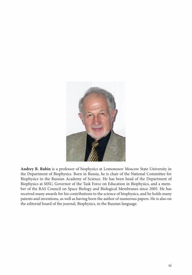
Andrey B. Rubin is a professor of biophysics at Lomonosov Moscow State University in the Department of Biophysics. Born in Russia, he is chair of the National Committee for Biophysics in the Russian Academy of Science. He has been head of the Department of Biophysics at MSU, Governor of the Task Force on Education in Biophysics, and a mem-ber of the RAS Council on Space Biology and Biological Membranes since 2005. He has received many awards for his contributions to the science of biophysics, and he holds many patents and inventions, as well as having been the author of numerous papers. He is also on the editorial board of the journal, Biophysics, in the Russian language.

Th e book does not forgive you for being lazy, And like a hoover, will refresh your brain. Its aim is not to make you go crazy But save your gyri from chondrosis pain.
IntroductionBiophysics is a science about physical and physicochemical interactions which lie in the basis of biological processes. Modern theoretical constructions and biophysical models are based on physical notions of energy, force, types of interactions, on general principles of physical and formal kinetics, thermodynamics and information theory. Th ese notions refl ect the nature of fundamental interactions and laws of motion of matter that is the sub-ject of physics as a basic natural science. As a biological science, biophysics has biological processes and phenomena in the focal point of its interests. Th e key challenge for up-to-date biophysics is the insight into the deepest elemental levels, which comprise the molecular basis of the structural organization of living organisms.
Th e present stage of biophysics development is characterized by principal advances, associated fi rst of all with the great progress in biophysics of complex systems and molecu-lar biophysics. It is namely in these fi elds, studying the laws of dynamic behavior of biologi-cal systems and mechanisms of molecular interaction in biological structures, that general results were obtained and then used to form the general theoretical basis of biophysics. Main ideas developed in such parts of biophysics as kinetics, thermodynamics, the the-ory of regulation of biological systems, structures of biopolymers and their electronic and conformational properties, provide a deep insight intomechanisms of important biological processes.
At the same time, the specifi city of biological systems is also displayed in the unique-ness of the physical mechanisms of their molecular processes. A principal distinction is that specifi c parameters of elementary interactions can vary depending on the conditions in organisms where they proceed. For example, parameters of individual elementary acts of electron transfer in photosynthetic reaction centers not only change specifi cally in a life cycle, but vary also in diff erent types of plants distinguished by physiological and biochemi-cal parameters and fertility. Th is means that molecular interaction mechanisms do depend on the local environment in biological systems and are themselves exposed to the direct physiological and biochemical regulation. Th is forms an indissoluble connection between molecular interactions and characteristics of biological phenomena that develop on their basis. Th at is why studies of deep biophysicalmechanisms, associatedwith physiological and biochemical peculiarities of biological objects, are a base for practical application of the results of biophysical research. Suffi ce it to mention the development of diff erent meth-ods of early diagnostics of the state of biological systems, based on the data of molecular mechanisms of biological processes, which are widely used in diverse ranges of medicine and agriculture.
xv
xvi Introduction
In this book, the main ideas of modern biophysics are presented in the form accessible to wide circles of readers. Biophysics (biological physics) is a science about physical and physico-chemical mechanisms of interactions which lie in the basis of biological processes. Physical properties of biopolymers and kinetics of cell metabolic reactions are responsi-ble for molecular characteristics of biological processes. A biomacromolecule as the main structure element in a cell is considered in biophysics as a peculiar molecular machine where energy is transformed and conversed from one type of energy into another. It is pertinent to recall what Bruce Alberts, a well-known American biologist, said about a cell. Hewrote that “the entire cell can be viewed as a factory that contains an elaborate network of interlocking assembly lines, each of which is composed of a set of large protein machines” (Cell, 1998, vol. 92, pp. 291–294).
Th e real understanding of how these protein machines operate demands the knowledge of not only atomic equilibrium structure, but also our understanding of kinetic and energy characteristics of intermediate transformations. In the postgenome sequencing era, the fi rst priority is given to the mechanisms of intramolecular mobility of macromolecular com-plexes as the base of their activity. Such an approach corresponds to the biophysical concept of directed electron-conformational interactions when energy transformation and reaction product generation become a result of internal interaction between separate parts within the whole macromolecular complex. In other words, this is the concept of a “physicalmachine” put forward in the 1970–1980s by D. S.Chernavsky, L.A. Blumenfeld, and M.V.Volkelshtein.
In theoretical biophysics, generalized kinetic and physical models of interactions allow us to describe diff erent biological phenomena. However, the analysis of such models clearly demonstrates that diff erent biological processes can very oft en be similar with respect to their molecular mechanisms. For example, mechanisms of primary photobiological pro-cesses (photosynthesis, visual reception), enzyme catalysis in the enzyme active center, and ion transfer through membrane channels are governed by similar physical principles. It fol-lows that educational programs for biology at universities should necessarily include ideas of physics, mathematics and physical chemistry, thus illustrating their effi ciency in solving biological problems. Biophysics bears the main responsibility of showing the important role of the regular application of ideas from exact sciences in studying biological processes.
PART I
BIOPHYSICSOF COMPLEX SYSTEMS

IKinetics of Biological Processes
1Qualitative Methods
for Studying Dynamic Modelsof Biological Processes
2Types of Dynamic Behavior
of Biological Systems
3Kinetics of Enzyme Processes
4Self-organization Processes
in Distributed Biological Systems

5
1Qualitative Methodsfor Studying Dynamic Modelsof Biological Processes
The functioning of the integrated biological system is a result of interactions of itscomponents in time and space. Elucidation of the principles of regulation of sucha system is a problem that can be solved only with the use of correctly chosenmathematical methods.
The kinetics of biological processes includes the time-dependent behavior ofvarious processes proceeding at different levels of life organization: biochemicalconversions, generation of electric potentials on biological membranes, cell cycles,accumulation of biomass or species reproduction, interactions of living populationsin biocommunities.
1.1 General Principles of Descriptionof Kinetic Behavior of Biological Systems
The kinetics of a system is characterized by a totality of variables and parametersexpressed via measurable quantities, which at each instant of time have definite
numerical values. �
In different biological systems, different measurable values can play the roleof variables: those are concentrations of intermediate substances in biochemistry,
6 Compendium of Biophysics
the number of microorganisms or their overall biomass in microbiology, the speciespopulation number in ecology, membrane potentials in biophysics of membraneprocesses, etc. Parameters may be temperature, humidity, pH, electric conductanceof membranes, etc.
This is sufficient to construct a general mathematical model representing a systemof n differential equations:
dc1/dt = f1(c1 , . . . , cn);. . . . . . . . . . . . . . . . . . . . . .
dcn/dt = fn(c1, . . . , cn) ,(1.1)
where c1(t), . . . , cn(t) are unknown functions of time describing the system variables(for example, substance concentrations); dci/dt are rates of changes of these vari-ables; fi are functions dependent on external and internal parameters of the system.A comprehensive model of type (1.1) may contain a large number of equations,including nonlinear ones.
Many essential questions concerning the qualitative character of the system behav-ior, in particular, stability of stationary states and transition between them, oscillationmodes and others, can be solved using methods of the qualitative theory of differen-tial equations. These methods permit revealing important general properties of themodel without determining explicitly the unknown functions c1(t), . . . , cn(t). Suchan approach gives good results when analyzing the models that consist of a smallnumber of equations and reflect the most important dynamic features of the system.
The key approach in the qualitative theory of differential equations is to character-ize the state of the system as a whole by variables c1, c2 , . . . , cn, which they aquireat each instant of time upon changing in accord with (1.1). If the values of vari-ables c1, c2, . . . , cn are put on rectangular coordinate axes in the n-dimensional space,the system state will be described by some point M in this space with coordinatesM(c1, c2, . . . , cn). The point M is called a representation point.
The change in the system state is comparable to the displacement of the point Min the n-dimensional space. The space with coordinates c1, c2, . . . , cn is a phase state;the curve, described in it by the point M, is a phase trajectory.
1.2 Qualitative Analysis of Elementary Modelsof Biological Processes
Let us consider qualitative methods of studying such systems represented asa system of two independent differential equations (the right-hand parts do not
depend explicitly on time), that can be written as:
dx /dt = P (x , y), dy /dt = Q(x , y). � (1.2)
Here P (x , y) and Q(x , y) are continuous functions, determined in some range Gof the Euclidean plane (x and y are Cartesian coordinates) and having continuousderivatives not lower than the first order.
The range may be both unlimited and limited. When variables x and y havea certain biological meaning (substance concentrations, species population number),
Qualitative Methods for Studying Dynamic Models 7
some restrictions are usually superimposed on them. First of all, biological variablescannot be negative.
Accept the coordinates of the representation point M0 to be (x0 , y0) at t = t0.At every next instant of time t, the representation point will move in compli-
ance with the system of equations (1.2) and have the positionM(x , y), correspondingto x(t), y(t). The set of points on the phase plane x , y is a phase trajectory. �
The character of phase trajectories reflects general qualitative features of thesystem behavior in time. The phase plane, divided in trajectories, represents an easilyvisible “portrait” of the system. It allows grasping at once the whole set of possi-ble motions (changes in variables x , y ) corresponding to the initial conditions. Thephase trajectory has tangents, the slopes of which in every point M(x , y) equals thederivative value in this point dy /dx . Accordingly, to trace a phase trajectory throughpoint M1(x1 , y1) of the phase plane, it is enough to know the direction of the tangentin this point of the plane or the value of the derivative
dy
dx x= x1y= y1
.
To this end, it is required to have an equation with variables x , y andwithout time tin an explicit form. For that, let us divide the second equation in system (1.2) by thefirst one. The following differential equation is obtained
dy
dx= Q(x , y)
P (x , y), (1.3)
which is frequently much more simple than the initial system (1.2). Solution of equa-tion (1.3) y = y(x , c) or in an explicit form F (x , y) = C , where C is the constant ofintegration, yields a family of integral curves — phase trajectories of system (1.2) onthe plane x , y .
But generally, equation (1.3) may have no analytical solution, and then integralplotting should be done using qualitative methods.
Method of Isoclinic Lines. The method of isoclinic lines is typically used forqualitative plotting of a phase portrait of a system. In this case, lines, which
intersect the integral lines at a certain angle, are plotted on the phase plane. Theanalysis of a number of isoclinic lines can show the probable course of the integrallines. �
The equation of isoclinic lines can be obtained from equation (1.3). Supposedy /dx = A, where A is a definite constant value. The value of A is a slope of thetangent to the phase trajectory and, consequently, can have values from −∞ to +∞.Substituting the A value instead of dy /dx in (1.3), we get the equation of isocliniclines:
A =Q(x , y)P (x , y)
. (1.4)
By giving different definite numeric values to A, we obtain a family of curves. Inany point of each of these curves, the tangent slope to the phase trajectory, passingthrough this point, is the same value, namely the value of A, which characterizes thegiven isoclinic line.
8 Compendium of Biophysics
Note that in the case of linear systems, i.e. systems of the type
dx/dt = ax + by , dy /dt = cx + dy , (1.5)
isoclinic lines represent a bundle of straight lines, passing through the origin ofcoordinates:
cx + dy
ax + by= A or y = (Aa − c)x
d − Ab.
Singular Points. Equation (1.3) determines directly the singular tangent to thecorresponding integral curve in each point of the plane. Exclusion is the point ofintersection of all isoclinic lines (x, y ), at which the tangent direction is indefinite,because in this case the value of the derivative is ambiguous:
dy
dx x= xy= y
= Q(x , y)P (x , y)
= 00
.
The points, in which time derivatives of variables x and y turn concurrently to zero
dx
dt x ,y= P (x , y) = 0, dy
dt x ,y= Q(x , y) = 0 (1.6)
and in which the direction of tangents to integral curves is indefinite, are singularpoints. The singular point in the equation of phase trajectories (1.3) complies withthe stationary state of system (1.2), because the rates of changes of variables in thispoint are equal to zero, and its coordinates are stationary values of variables x , y .
For a qualitative study of a system, it is often possible not to go beyond plottingonly some isoclinic lines on the phase plane. Of special interest are the so-called
basic isoclinic lines: dy /dx = 0 is the isoclinic line of horizontal tangents to phasetrajectories, the equation of which is Q(x , y) = 0, and the isoclinic of vertical tangentsdy /dx = ∞, which is in line with equation P (x , y) = 0. �
The plotting of the basic isoclinic lines and the determination of their intersectionpoint, the coordinates of which satisfy the following conditions
P (x , y) = 0, Q(x , y) = 0, (1.7)
gives the intersection point of all isoclinic lines on the phase plane. As mentionedabove, this point is a singular point and corresponds to the stationary state of thesystem (Fig. 1.1).
Figure 1.1 demonstrates the case of one stationary point of intersection of basicisoclinic lines of the system. The figure shows directions of the tangents dy /dx to thetrajectories on the phase plane.
The number of stationary states in system of equations (1.2) is equal to the numberof intersection points of basic isoclinic lines on the phase plane.
Stability of Stationary States. Assume the considered system to be in the equi-librium state. Then the representation point on the phase plane is stationary in oneof the singular points of the equation of integral curves (1.3), because, by definition,in these points dx/dt = 0, dy /dt = 0.
Qualitative Methods for Studying Dynamic Models 9
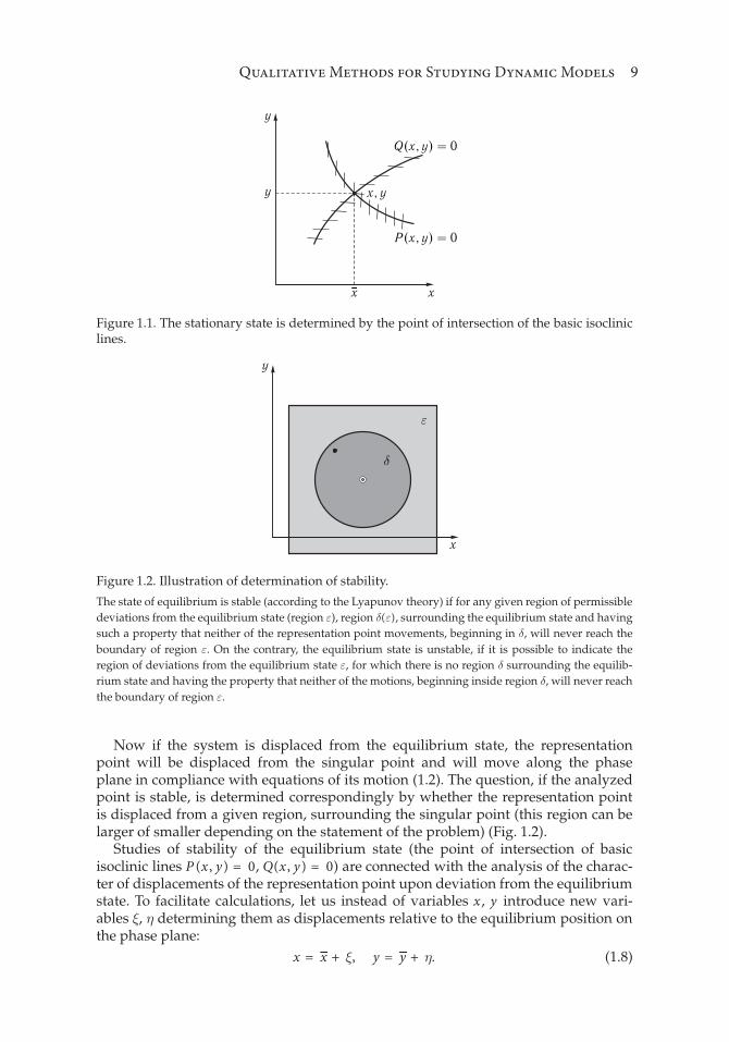
Figure 1.1. The stationary state is determined by the point of intersection of the basic isoclinic
lines.
Figure 1.2. Illustration of determination of stability.
The state of equilibrium is stable (according to the Lyapunov theory) if for any given region of permissible
deviations from the equilibrium state (region ), region ( ), surrounding the equilibrium state and having
such a property that neither of the representation point movements, beginning in , will never reach the
boundary of region . On the contrary, the equilibrium state is unstable, if it is possible to indicate the
region of deviations from the equilibrium state , for which there is no region surrounding the equilib-
rium state and having the property that neither of the motions, beginning inside region , will never reach
the boundary of region .
Now if the system is displaced from the equilibrium state, the representationpoint will be displaced from the singular point and will move along the phaseplane in compliance with equations of its motion (1.2). The question, if the analyzedpoint is stable, is determined correspondingly by whether the representation pointis displaced from a given region, surrounding the singular point (this region can belarger of smaller depending on the statement of the problem) (Fig. 1.2).
Studies of stability of the equilibrium state (the point of intersection of basicisoclinic lines P (x , y) = 0, Q(x , y) = 0) are connected with the analysis of the charac-ter of displacements of the representation point upon deviation from the equilibriumstate. To facilitate calculations, let us instead of variables x , y introduce new vari-ables , determining them as displacements relative to the equilibrium position onthe phase plane:
x = x + , y = y + . (1.8)
10 Compendium of Biophysics
Substituting these expressions in (1.2), we get
dx/dt + d /dt = P (x + , y + ),dy/dt + d /dt = Q(x + , y + ),
dx/dt = dy /dt = 0, because x , y are the coordinates of the singular point.
(1.9)
Let us factorize the right-hand side of the above equations in Taylor series by vari-ables , and cast out nonlinear members. The following system of linear equationswill be obtained:
d /dt = a + b , d /dt = c + d , (1.10)
where coefficients a, b, c , and d are values of quotient derivatives in point (x , y):
a = P ′x (x , y), b = P ′y (x , y), c = Q′x(x , y), d = Q′y (x , y).
System (1.10) is called a linearized system or the system of the first approxima-tion. �
For a large class of systems, namely structurally stable, or “rough” systems, thecharacter of phase trajectories near singular points is preserved at any sufficientlysmall changes in the right-hand side of equations (1.2) — functions P and Q, if thechanges in the derivatives of these functions are also small. For such systems, studiesof equations of the first approximation (1.10) give a correct answer to the question onthe stability of the equilibrium state of system (1.2) and on the topological structureof the phase plane near this equilibrium state.
System (1.10) is a linear one, and therefore its analytical solution is possible. Thegeneral solution of the system is found as follows:
= Ae t , = Be t . (1.11)
By substitution of these expressions in (1.10) and reduction of the obtained expres-sions by e t , the following expression is obtained:
A = aA + bB , B = cA + dB . (1.12)
Algebraic system of equations (1.12) with unknown members A and B has, asknown, a nonzero solution only if its determinant, consisting of coefficients at theunknown members, is zero:
a − b
c d − = 0.
Having uncovered this determinant, we get the so-called characteristic equationof the system:
2 − (a + d) + (ad − bc) = 0. � (1.13)
The solution of this equation yields indices 1,2 at which nonzero solutions for Aand B of system (1.12) are possible:
1,2 = a + d
2± (a + d)2
4+ bc − ad . (1.14)
Qualitative Methods for Studying Dynamic Models 11
If the radicand is negative, 1,2 are complex conjugate values. Let us assume thatboth roots of equation (1.13) have real numbers varying from zero, and there are nomultiple roots. Then the general solution of system (1.10) written as (1.11) may berepresented as a linear combination of exponents with indices 1 and 2 :
= C11e 1t + C12e 2t , = C21e 1t + C22e 2t . (1.15)
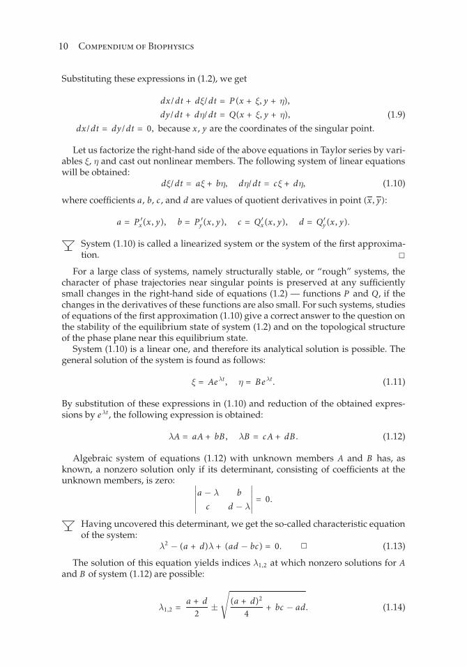
The behavior of variables , , in compliance with (1.15) and, consequently, thebehavior of variables x and y near the singular point (x , y) depend on the type ofindices of the exponents 1 and 2 . When the indices 1 and 2 are real and have thesame sign, the singular point is called a node (Fig. 1.3).
Figure 1.3. Stable (I) and unstable (II) nodes on phase plane.
If 1,2 < 0, the values of variables , (deviations from the equilibrium position) decrease with time. In
this case, singular point (x , y) is a stable node (I). If 1,2 > 0, values , increase with time and the singular
point is an unstable node (II).
Many biological systems are characterized by a “non-oscillatory” transition froman arbitrary initial state to the stationary one, which corresponds to a stationarysolution of the stable node type in the model.
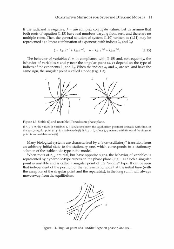
When roots of 1,2 are real, but have opposite signs, the behavior of variables isrepresented by hyperbolic-type curves on the phase plane (Fig. 1.4). Such a singularpoint is unstable and is called a singular point of the “saddle” type. It can be seenthat independent of the position of the representation point at the initial time (withthe exception of the singular point and the separatrix), in the long run it will alwaysmove away from the equilibrium.
Figure 1.4. Singular point of a “saddle” type on phase plane (xy).
12 Compendium of Biophysics
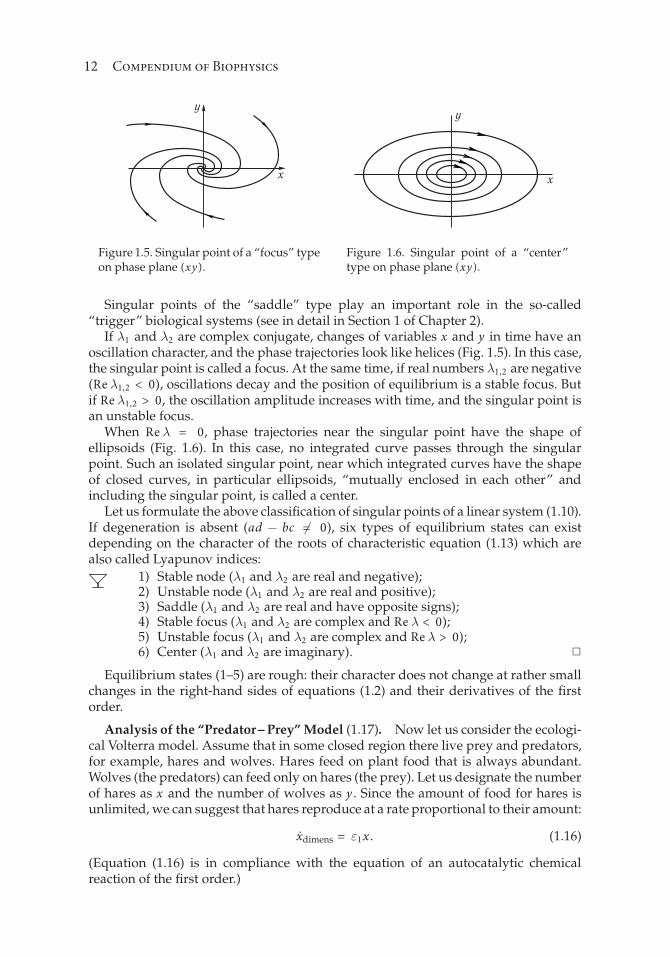
Figure 1.5. Singular point of a “focus” type
on phase plane (xy).Figure 1.6. Singular point of a “center”
type on phase plane (xy).
Singular points of the “saddle” type play an important role in the so-called“trigger” biological systems (see in detail in Section 1 of Chapter 2).
If 1 and 2 are complex conjugate, changes of variables x and y in time have anoscillation character, and the phase trajectories look like helices (Fig. 1.5). In this case,the singular point is called a focus. At the same time, if real numbers 1,2 are negative(Re 1,2 < 0), oscillations decay and the position of equilibrium is a stable focus. Butif Re 1,2 > 0, the oscillation amplitude increases with time, and the singular point isan unstable focus.
When Re = 0, phase trajectories near the singular point have the shape ofellipsoids (Fig. 1.6). In this case, no integrated curve passes through the singularpoint. Such an isolated singular point, near which integrated curves have the shapeof closed curves, in particular ellipsoids, “mutually enclosed in each other” andincluding the singular point, is called a center.
Let us formulate the above classification of singular points of a linear system (1.10).If degeneration is absent (ad − bc �= 0), six types of equilibrium states can existdepending on the character of the roots of characteristic equation (1.13) which arealso called Lyapunov indices:
1) Stable node ( 1 and 2 are real and negative);2) Unstable node ( 1 and 2 are real and positive);3) Saddle ( 1 and 2 are real and have opposite signs);4) Stable focus ( 1 and 2 are complex and Re < 0);5) Unstable focus ( 1 and 2 are complex and Re > 0);6) Center ( 1 and 2 are imaginary). �
Equilibrium states (1–5) are rough: their character does not change at rather smallchanges in the right-hand sides of equations (1.2) and their derivatives of the firstorder.
Analysis of the “Predator– Prey”Model (1.17). Now let us consider the ecologi-cal Volterra model. Assume that in some closed region there live prey and predators,for example, hares and wolves. Hares feed on plant food that is always abundant.Wolves (the predators) can feed only on hares (the prey). Let us designate the numberof hares as x and the number of wolves as y . Since the amount of food for hares isunlimited, we can suggest that hares reproduce at a rate proportional to their amount:
xdimens = 1x . (1.16)
(Equation (1.16) is in compliance with the equation of an autocatalytic chemicalreaction of the first order.)
Qualitative Methods for Studying Dynamic Models 13
Accept the loss in the number of hares to be proportional to the probability of theirencounter with wolves, i.e. proportional to the product x × y . The number of wolvesalso increases the faster, the more frequent their encounters with hares, i.e. propor-tional to x × y . In chemical kinetics, this corresponds to a bimolecular reaction, whenthe probability of appearance of a new molecule is proportional to the probabilityof encounter of two molecules, i.e. the product of their concentrations. In addition,natural death of wolves takes place, the rate of decrease in the number of speciesbeing proportional to their number. This is in compliance with the process of a chem-ical outflow from the reaction sphere. As a result, the following system of equationsis obtained for changes in the number of hares x and wolves y :
dx/dt = x( 1 − 1y), dy /dt = −y( 2 − 2x). (1.17)
Let us study the singular point in the Volterra predator-preymodel (1.17). Its coor-dinates are found promptly if the right-hand sides of equations in system (1.17) areequal to zero. This yields stationary non-zero values: x = 2/ 2 , y = 1/ 1 . As para-meters 1, 2, 1, 2 are positive, point (x , y) lies in the positive quadrant of the phaseplane. Linearization of this point yields
d
dt= − 1x = − 1 2
2; d
dt= − 2y = − 2 1
1.
Here (t), (t) are deviations from the singular point on the phase plane:
(t) = x(t) − x , (t) = y(t)− y .
The characteristic equation of the system is as follows:
− − 1 2
22 1
1−
= 0, 2 + 1 2 = 0.
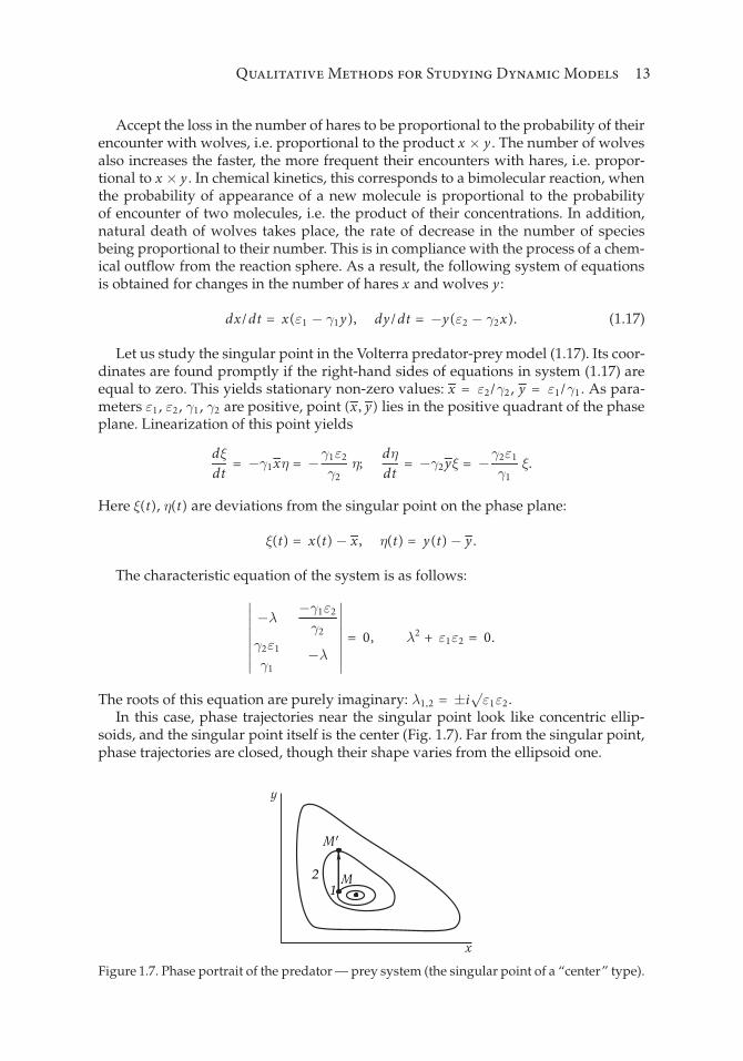
The roots of this equation are purely imaginary: 1,2 = ±i√ 1 2.In this case, phase trajectories near the singular point look like concentric ellip-
soids, and the singular point itself is the center (Fig. 1.7). Far from the singular point,phase trajectories are closed, though their shape varies from the ellipsoid one.
Figure 1.7. Phase portrait of the predator— prey system (the singular point of a “center” type).
14 Compendium of Biophysics
On the whole, the singular point of the “center” type is unstable. Let oscilla-tions x(t) and y(t) proceed so that the representation point moves along the phasetrajectory 1 (Fig. 1.7). At the instant of time when the point is in position M, sucha number of species Δy is added to the system from the outside that the representa-tion point jumps from point M to point M′. After that, if the system is again left onits own, oscillations x(t) and y(t) will occur with larger amplitudes than previously,and the representation point will move along trajectory 2. So, upon external actionthe oscillations change their characteristics forever.
Figure 1.8 shows plots of functions x(t) and y(t). It is seen that x(t) and y(t)are periodic functions of time, the maximum of the prey number surpassing themaximum of the number of predators.
Figure 1.8. Dependence of the number of predators y and prey x on time.
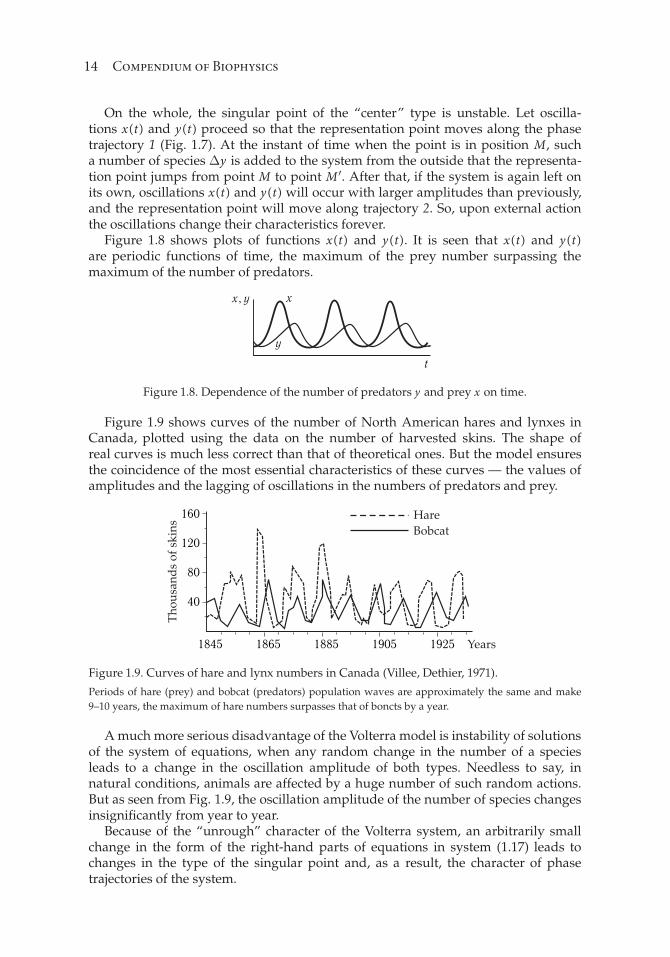
Figure 1.9 shows curves of the number of North American hares and lynxes inCanada, plotted using the data on the number of harvested skins. The shape ofreal curves is much less correct than that of theoretical ones. But the model ensuresthe coincidence of the most essential characteristics of these curves — the values ofamplitudes and the lagging of oscillations in the numbers of predators and prey.
Figure 1.9. Curves of hare and lynx numbers in Canada (Villee, Dethier, 1971).
Periods of hare (prey) and bobcat (predators) population waves are approximately the same and make
9–10 years, the maximum of hare numbers surpasses that of boncts by a year.
A much more serious disadvantage of the Volterra model is instability of solutionsof the system of equations, when any random change in the number of a speciesleads to a change in the oscillation amplitude of both types. Needless to say, innatural conditions, animals are affected by a huge number of such random actions.But as seen from Fig. 1.9, the oscillation amplitude of the number of species changesinsignificantly from year to year.
Because of the “unrough” character of the Volterra system, an arbitrarily smallchange in the form of the right-hand parts of equations in system (1.17) leads tochanges in the type of the singular point and, as a result, the character of phasetrajectories of the system.