Surya N. PatnaikOhio Aerospace Institute, Cleveland, Ohio

Rula M. Coroneos and Dale A. HopkinsGlenn Research Center, Cleveland, Ohio

Compatibility Conditionsof Structural Mechanics

NASA/TM—1999-209175

November 1999

https://ntrs.nasa.gov/search.jsp?R=20000000252 2018-05-30T09:52:23+00:00Z

The NASA STI Program Office . . . in Profile

Since its founding, NASA has been dedicated tothe advancement of aeronautics and spacescience. The NASA Scientific and TechnicalInformation (STI) Program Office plays a key partin helping NASA maintain this important role.

The NASA STI Program Office is operated byLangley Research Center, the Lead Center forNASA’s scientific and technical information. TheNASA STI Program Office provides access to theNASA STI Database, the largest collection ofaeronautical and space science STI in the world.The Program Office is also NASA’s institutionalmechanism for disseminating the results of itsresearch and development activities. These resultsare published by NASA in the NASA STI ReportSeries, which includes the following report types:

• TECHNICAL PUBLICATION. Reports ofcompleted research or a major significantphase of research that present the results ofNASA programs and include extensive dataor theoretical analysis. Includes compilationsof significant scientific and technical data andinformation deemed to be of continuingreference value. NASA’s counterpart of peer-reviewed formal professional papers buthas less stringent limitations on manuscriptlength and extent of graphic presentations.

• TECHNICAL MEMORANDUM. Scientificand technical findings that are preliminary orof specialized interest, e.g., quick releasereports, working papers, and bibliographiesthat contain minimal annotation. Does notcontain extensive analysis.

• CONTRACTOR REPORT. Scientific andtechnical findings by NASA-sponsoredcontractors and grantees.

• CONFERENCE PUBLICATION. Collectedpapers from scientific and technicalconferences, symposia, seminars, or othermeetings sponsored or cosponsored byNASA.

• SPECIAL PUBLICATION. Scientific,technical, or historical information fromNASA programs, projects, and missions,often concerned with subjects havingsubstantial public interest.

• TECHNICAL TRANSLATION. English-language translations of foreign scientificand technical material pertinent to NASA’smission.

Specialized services that complement the STIProgram Office’s diverse offerings includecreating custom thesauri, building customizeddata bases, organizing and publishing researchresults . . . even providing videos.

For more information about the NASA STIProgram Office, see the following:

• Access the NASA STI Program Home Pageat http://www.sti.nasa.gov

• E-mail your question via the Internet tohelp@sti.nasa.gov

• Fax your question to the NASA AccessHelp Desk at (301) 621-0134

• Telephone the NASA Access Help Desk at(301) 621-0390

• Write to: NASA Access Help Desk NASA Center for AeroSpace Information 7121 Standard Drive Hanover, MD 21076

Surya N. PatnaikOhio Aerospace Institute, Cleveland, Ohio

Rula M. Coroneos and Dale A. HopkinsGlenn Research Center, Cleveland, Ohio

Compatibility Conditionsof Structural Mechanics

NASA/TM—1999-209175

November 1999

National Aeronautics andSpace Administration

Glenn Research Center

Acknowledgment

The authors have benefited from discussion with Dr. Michael J. Zeheof NASA Glenn Research Center and express their gratitude to him.

Available from

NASA Center for Aerospace Information7121 Standard DriveHanover, MD 21076Price Code: A03

National Technical Information Service5285 Port Royal RoadSpringfield, VA 22100

Price Code: A03

NASA/TM—1999-209175 1

Compatibility Conditions of Structural Mechanics

SURYA N. PATNAIKOhio Aerospace Institute22800 Cedar Point Rd.

Brook Park, Ohio 44142

RULA M. CORONEOS AND DALE A. HOPKINSNational Aeronautics and Space Administration

Glenn Research CenterCleveland, Ohio 44135

SYMBOLS

A internal energy

a, b plate radii

avx, avy, avz direction cosines

B complementary energy

B , B , Bx y z body force components

[B] equlibrium matrix

[C] compatibility matrix

E Young’s modulus

ex, ey eccentricities

{ F} internal force

[G} flexibility matrix

[J] deformation coefficient matrix

K plate rigidity

[K ] stiffness matrix

ø table height

Mr, Mϕ moments

P load

Px, Py, Pz reactions where displacements u v w, , and are prescribed

P P Px y z, , prescribed tractions

{ P} external load

{ P*} equivalent load

q uniformly distributed load

R1,…,R4 reactions along table legs

R redundant force

R residue function

r radius

NASA/TM—1999-209175 2

[S] IFM matrix

∆t temperature differential

u, v, w displacement components

V volume

W potential of work done

x, y, z Cartesian coordinates

β deformation

β0 initial deformation

γxy, γyz, γzx shear strain components

εx, εy, εz normal strain components

θx, θy rotations

ν Poisson’s ratio

πs variational functional

σx, σy, σz normal stress components

τxy, τyz, τzx shear stress components

ϕ1, ϕ2, ϕ3 stress functions

BCC boundary compatibility conditions

BMF Beltrami-Michell formulation

CBMF completed Beltrami-Michell formulation

CC compatibility conditions

DDR deformation displacement relations

EE equilibrium equations

IFM integrated force method

IFMD dual integrated force method

SUMMARY

The theory of elasticity has camouflaged a deficiency in the compatibility formulation since 1860. In structuresthe ad hoc compatibility conditions through virtual “cuts” and closing “gaps” are not parallel to the strain formula-tion in elasticity. This deficiency in the compatibility conditions has prevented the development of a direct stressdetermination method in structures and in elasticity. We have addressed this deficiency and attempted to unify thetheory of compatibility. This work has led to the development of the integrated force method for structures and thecompleted Beltrami-Michell formulation for elasticity. The improved accuracy observed in the solution of numericalexamples by the integrated force method can be attributed to the compliance of the compatibility conditions. Usingthe compatibility conditions allows mapping of variables and facile movement among different structural analysisformulations. This paper reviews and illustrates the requirement of compatibility in structures and in elasticity. Italso describes the generation of the conditions and quantifies the benefits of their use. The traditional analysismethods and available solutions (which have been obtained bypassing the missed conditions) should be verified forcompliance of the compatibility conditions.

NASA/TM—1999-209175 3

INTRODUCTION

The equilibrium equations and the compatibility conditions required for the analysis of stress in an elastic con-tinuum were formulated by Cauchy and Saint-Venant during the first and third quarters of the nineteenth century,respectively. Cauchy’s stress formulation was complete, with field equations and boundary conditions. Saint-Venantformulated the field equations in 1860 but did not provide the compatibility conditions on the boundary. Traditionalcompatibility theory in structures has been developed through the concept of redundant forces, with virtual “cuts”and subsequent closing of the “gaps.” In elasticity the field equations generated through Saint-Venant’s strain for-mulation are not parallel to the concept of cuts and closed gaps in structures. The compatibility formulation differedin elasticity and in structures. In other words, compatibility theory has concealed a weak spot since the strain formu-lation in 1860. The deficiency has prevented the development of a direct structural analysis method, even though theorigin of the science can be traced back to the cantilever experiment of Galileo, conducted four centuries ago (ref. 1)

If compatibility is not required (as in the analysis of determinate structures), the method of forces represents themost efficient formulation. This method heretofore could not be extended to the analysis of indeterminate structuresbecause of the weakness in compatibility theory. The compatibility barrier blocked the natural growth of themethod, causing it to split into the stiffness method and the redundant force method as depicted in Fig. 1. The stiff-ness method has made magnificent progress, but the ad hoc redundant force formulation has disappeared for allpractical purposes because of its limited scope (refs. 2 and 3).

Our research has attempted to extend the method of forces to the analysis of indeterminate structures. The basicconcept of the method is expressed in the following symbolic equation (devised through discussions with Richard H.Gallagher):

Equilibrium equation

Compatibility conditionStress

Mechanical load

Initial deformation(1)

{ } =

For stress analysis the equilibrium equation (EE) represents the necessary condition. Sufficiency is achieved throughthe compatibility conditions (CC). Even though a method corresponding to equation (1) could not be developed,such a formulation was envisioned by Michell and is described by Love (ref. 4) in the following quotation:

It is possible by taking account of these relations [compatibility conditions] to obtain a completesystem of equations [eq. (1)] which must be satisfied by stress components, and thus the way isopen for a direct determination of stress without the intermediate steps of forming and solvingdifferential equations to determine the components of displacements.

At the turn of the twentieth century Beltrami and Michell attempted to formulate a direct method in elasticitywith stress {σ} as the unknown, referred to as the Beltrami-Michell formulation (BMF). Its field equation (L {σ} ={P}), was obtained by coupling the EE and the CC. The BMF had limited scope because the compatibility condi-tions on the boundary were not treated. For discrete structural analysis a method that can be considered parallel tothe BMF with internal force {F} as the unknown and the governing equation ([S]{ F}) = { P} was not availableduring the formative 1960’s.

We have addressed and attempted to unify compatibility theory in elasticity and in structures. In elasticity thecompatibility conditions on the boundary have been identified (refs. 5 and 6). In structures our compatibility condi-tions are analogous to the strain formulation (ref. 7). Coupling the compatibility conditions to the equilibrium equa-tions has led to the formulation of the integrated force method (IFM, ref. 8) for finite element structural analysis andthe completed Beltrami-Michell formulation (CBMF) in elasticity (ref. 6). Both IFM and CBMF are versatile formu-lations applicable to static and dynamic analysis of linear and nonlinear structures. These methods and other analysisformulations are summarized in Table I. The IFM equations can be specialized to obtain the stiffness method (refs. 9and 10) and the classical force method (ref. 11). Through the IFM matrices the hybrid and total formulations can bedefined. The variational functional of the integrated force method can be specialized to obtain the functionals of theother methods given in Table I. The IFM equations allow free movement from stress to displacement and vice versa.

This paper is an invited paper in the International Journal of Numerical Methods in Engineering commemorat-ing Richard H. Gallagher (1927–1997), who was a co-contributor to the theory of the integrated force method(refs. 7, 8, and 12). The paper reviews and illustrates the requirement of compatibility in structures and in elasticity.

NASA/TM—1999-209175 4

It discusses the role of compatibility in structures by considering Navier’s table problem as an example. It also illus-trates the necessity of the boundary compatibility conditions in elasticity through the analysis of a composite plate.We generated the three-dimensional compatibility conditions on the boundary from the stationary conditions of theIFM variational functional. We also quantified the benefits from their use in structural analysis by solving threeexamples. The paper is completed with discussions and conclusions.

REQUIREMENT OF COMPATIBILITY CONDITIONS

A direct determination of the six stress components requires six equations—three equilibrium equations andthree compatibility conditions. However, indirect methods can be obtained by transforming stress into displacementor scalar function. The indirect methods emphasize either equilibrium equations or compatibility conditions. How-ever, confirming the accuracy of the response generated by the direct or indirect methods requires satisfying the EEand the CC. Likewise, analysis of indeterminate structures requires both equilibrium and compatibility. The require-ment of compatibility is illustrated by considering both Navier’s table problem for structures and a composite circu-lar plate in elasticity.

Navier’s Table Problem

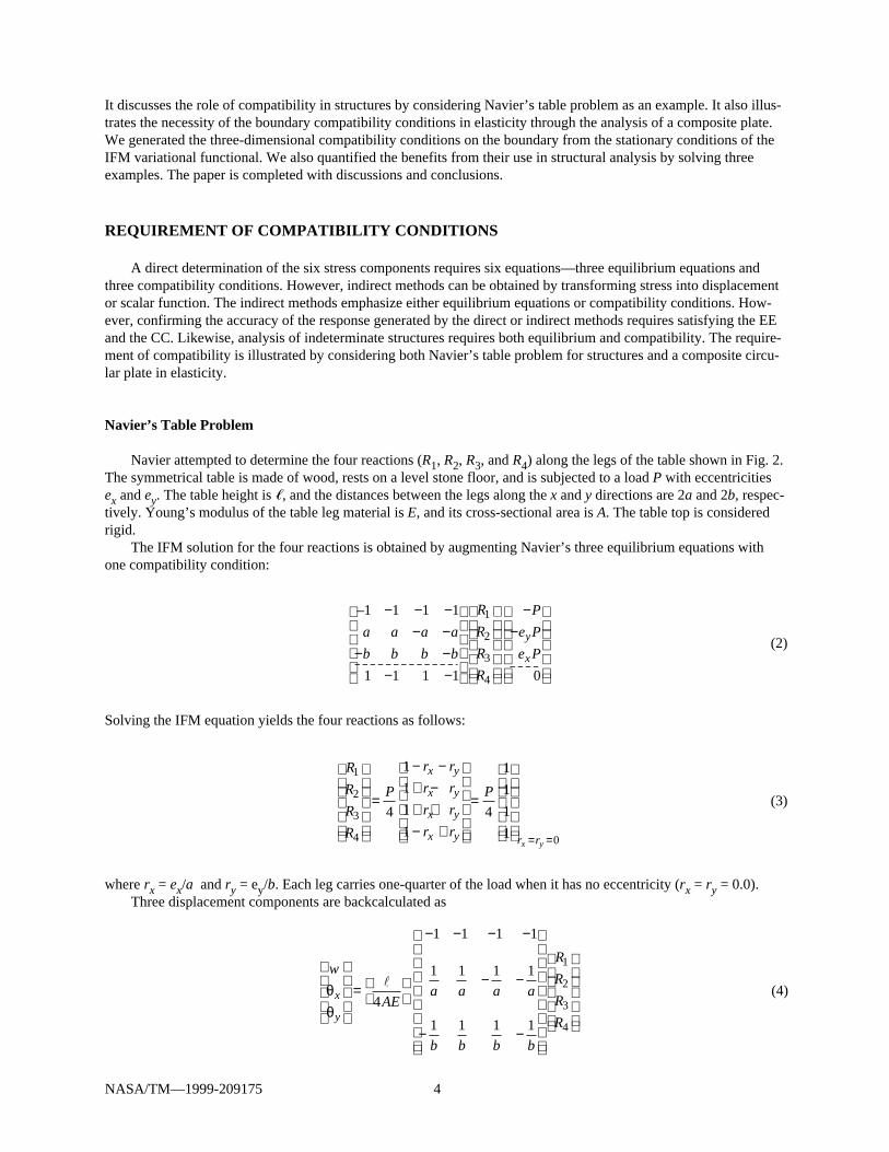
Navier attempted to determine the four reactions (R1, R2, R3, and R4) along the legs of the table shown in Fig. 2.The symmetrical table is made of wood, rests on a level stone floor, and is subjected to a load P with eccentricitiesex and ey. The table height is ø, and the distances between the legs along the x and y directions are 2a and 2b, respec-tively. Young’s modulus of the table leg material is E, and its cross-sectional area is A. The table top is consideredrigid.

The IFM solution for the four reactions is obtained by augmenting Navier’s three equilibrium equations withone compatibility condition:

–1 1 1 1

1 1 1 1 0

1

2

3

4

− − −− −

− −− −

−−

a a a a

b b b b

R

R

R

R

P

e P

e Py

x(2)

Solving the IFM equation yields the four reactions as follows:

R

R

R

R

P

r r

r r

r r

r r

P

x y

x y

x y

x y r rx y

1

2

3

4 0

4

1

1

1

14

1

1

1

1

=

− −+ −+ +− +

=

= =

(3)

where rx = ex/a and ry = ey/b. Each leg carries one-quarter of the load when it has no eccentricity (rx = ry = 0.0).Three displacement components are backcalculated as

w

AEa a a a

b b b b

R

R

R

R

x

y

θθ

=

− − − −

− −

− −

l

4

1 1 1 1

1 1 1 1

1 1 1 1

1

2

3

4

(4)

NASA/TM—1999-209175 5

If the table had three legs, its three reactions could have been calculated from the three equilibrium equations. Itsfourth leg requires an additional compatibility condition. The IFM through its compatibility formulation provides thefourth equation in the matrix (see eq. (2)).

Instead of developing the compatibility condition Navier rewrote the three equilibrium equations in terms of thedisplacements (w, θx, and θy) to obtain the three stiffness equations. Solution yielded the three displacements, fromwhich the four reactions could be backcalculated. Generalization of this procedure, which is credited to Navier,became the popular stiffness method (refs. 13 and 14).

In the redundant force method one leg of the table was “cut” to obtain a three-legged determinate table. Thisdeterminate problem was solved for reactions and displacement ∆P at the cut. The solution process was repeated fora load R, called a redundant force, in place of the reaction for the leg that had been cut. The resulting displacement∆R at the cut was obtained. Because the physical table had no real cut, the gap was closed (∆P + ∆R = 0), yieldingthe value of the redundant reaction. Solving the determinate structure subjected to both the redundant reaction andthe external load provided the result for the indeterminate problem. The generalization of this procedure became theredundant force method (refs. 2, 3, and 15).

Composite Circular Plate

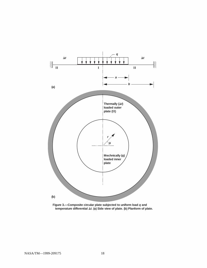
The compatibility requirement in elasticity is illustrated through the example of a composite circular plate asshown in Fig. 3. The structure is made of an aluminum inner plate (I) of radius a = 6 in. and a steel outer sector (II)of radius b = 12 in. The inner plate (I) is subjected to a uniformly distributed load of intensity q = 100 psi, whereasthe outer plate (II) is uniformly heated with a temperature differential of ∆t = 50 °F. The thicknesses of the inner andouter plates are hI = 0.2 in. and hII = 0.15 in., Young’s moduli are EI = 10.6×106 and EII = 30.0×106 psi, Poisson’sratios are νI= 0.33 and νII = 0.3, respectively, the coefficient of expansion of the outer plate is αt.

In the completed Beltrami-Michell formulation the moments Mr and Mϕ are considered as the unknowns. Theplate has one field equilibrium equation and one compatibility condition as follows:

d

drrM

dM

drrqr

2

2 0( ) − + =ϕ(5)

rd

drM M M M Kr

h

d t

drr rt

ϕ ϕν ν α−( ) + +( ) −( ) +

=1 0

∆(6)

where the plate rigidity is defined as K = Eh3/[12(1 – ν2)]. Solving the composite problem requires solving the twofield equations for the six boundary conditions. One boundary compatibility condition occurs at the clamped bound-ary (r = b):

10

KM M

t

hr t

II

ϕ ν α−( ) +

=∆(7)

Three boundary conditions occur at the interface (r = a):

M MrI

rII= (8a)

d

drrM M

d

drrM Mr

I

r

II

( ) −

= ( ) −

ϕ ϕ (8b)

1 1

KM M

t

h KM M

t

hr t

I

r t

II

ϕ ϕν α ν α−( ) +

= −( ) +

∆ ∆(8c)

NASA/TM—1999-209175 6

where the superscripts I and II refer to the two plate sectors at the interface. At the origin (r = 0)

Moments are finite: (8d)M MIrI

ϕ ,( )Solving the field equations yields moments for the inner plate as follows:

M rB

rC r C D qrr

I I I I( ) log (9a)= − + +( ) + −( ) + − +( )12 1 1 1

21

21

1

41

1

2

1

163ν ν ν

M rB

rC r C D qrI I I I

ϕ ν ν ν( ) log (9b)= − + +( ) − −( ) + − +( )12 1 1 1

21

21

1

41

1

2

1

161 3

Likewise, solving for the outer plate with no distributed load gives

M rB

rC r C Dr

II II II( ) log (1 a)= − + +( ) + −( ) +22 2 2 2

1

21

1

41

1

20ν ν

M rB

rC r C DII II II

ϕ ν ν( ) log (1 b)= − + +( ) − −( ) +22 2 2 2

1

21

1

41

1

20

The six constants (B1, B2, C1, C2, D1, and D2) are determined from the six boundary conditions. Substituting thenumerical values for the parameters yields the following moment solutions:

For the inner plate (0 ≤ r ≤ a)

M r rrI ( ) ( a)= −844 05 20 81 112. .

M r rIϕ ( ) ( b)= −844 05 12 44 112. .

For the outer plate (a ≤ r ≤ b)

M r r rrII ( ) log ( c)= − ( ) −2046 63 5203 06 1170 112. . /

M r r rIIϕ ( ) log ( d)= + ( ) −2676 63 5203 06 1170 112. . /

The displacement, if required, is obtained by integrating the deformation displacement relations. Calculating theintegration for the constraints required using the kinematic boundary equations (refs. 16 and 17). The transversedisplacements for the plate are as follows (ref. 16):

For the inner plate (0 ≤ r ≤ a)

w r rI ( ) (12a)r = − + × −3 1209 0 0356 0 1757 102 3 4. . .

For the outer plate (a ≤ r ≤ b)

w r r r rII ( ) log log (12b)r = − − +5 3614 0 1344 0 7296 0 044172 2. . . .

NASA/TM—1999-209175 7

The CBMF required the boundary compatibility conditions given by equations (7) and (8c). Because these condi-tions were not available, the CBMF could not be developed earlier. The CBMF can be transformed to obtainNavier’s displacement method (ref. 18).

GENERATION OF COMPATIBILITY CONDITIONS

Strain, or deformation balance, represents the physical concept behind the compatibility conditions, which arecontroller type of relations. In elasticity the strains ε are controlled, f(εx, εy, …, γzx) = 0; or in structures the defor-mations β are balanced, f(β1, β2, …, βn) = 0. The compatibility conditions are generated here first for elasticity andthen for structures.

Generation of Compatibility Conditions in Elasticity

The field compatibility conditions can be derived by eliminating the displacements from the strain displacementrelations (ref. 19). This technique has not yet been successfully extended to deriving the boundary compatibilityconditions (BCC). At present the BCC have been generated from the stationary condition of the IFM variationalfunctional. This functional πs has three terms: A, B, and W. For three-dimensional elasticity πs has the followingexplicit form:

πs A B W= + − (13)

Term A represents the internal energy expressed in terms of stresses and displacements.

Au

x

v

y

w

z

u

y

v

x

v

z

w

y

u

z

w

xdVx y z xy yz zx= ∂

∂+ ∂

∂+ ∂

∂+ ∂

∂+ ∂

∂

+ ∂∂

+ ∂∂

+ ∂∂

+ ∂∂

∫ σ σ σ τ τ τ

volume

(14a)

Term B represents the complementary energy. This term, expressed in terms of strain and stress function, has thefollowing form:

By z z x x y x y y zx y z xy xy= ∂

∂+ ∂

∂

+ ∂

∂+ ∂

∂

+ ∂

∂+ ∂

∂

+ − ∂

∂ ∂

+ − ∂

∂ ∂

+

∫ ε ϕ ϕ ε ϕ ϕ ε ϕ ϕ τ ϕ γ ϕ23

2

22

2

21

2

23

2

22

2

21

2

23

21

volume

γγ ϕzx z x

dV− ∂∂ ∂

22 (14b)

Term W represents the potential of the work done due to the prescribed traction, displacement, and specified bodyforce:

W P u P v P w ds P u P v P w ds B u B v B w dVx y z x y z x y z= + +( ) + + +( ) + + +( )∫ ∫ ∫surface S surface S volume1 2

(14c)

where σx, σy, σz, τxy, τyz, and τzx are the six stress components; εx, εy, εz, γxy, γyz, and γzx are the six strain compo-

nents; u, v, and w are the three displacement components; ϕ1, ϕ2, and ϕ3 are the three stress functions;P P Px y z, , are

the three prescribed tractions; Px, Py, and Pz are reactions where displacements u v w, , and are prescribed; andB , B , Bx y z are the three body force components. The stress functions are defined as

NASA/TM—1999-209175 8

σ ϕ ϕ σ ϕ ϕ σ ϕ ϕ

τ ϕ τ ϕ τ ϕ

x y z

xy yz xz

y z z x x y

x y y z z x

= ∂∂

+ ∂∂

= ∂∂

+ ∂∂

= ∂∂

+ ∂∂

= − ∂∂ ∂

= − ∂∂ ∂

= − ∂∂ ∂

23

2

22

2

21

2

23

2

22

2

21

2

23

21

22

(15)

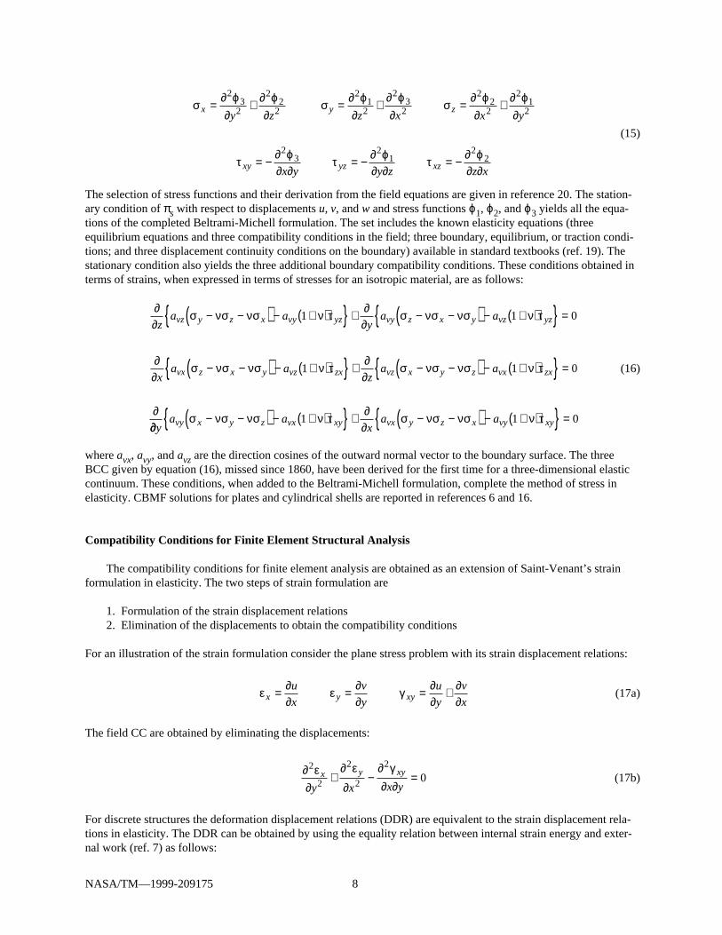
The selection of stress functions and their derivation from the field equations are given in reference 20. The station-ary condition of πs with respect to displacements u, v, and w and stress functions ϕ1, ϕ2, and ϕ3 yields all the equa-tions of the completed Beltrami-Michell formulation. The set includes the known elasticity equations (threeequilibrium equations and three compatibility conditions in the field; three boundary, equilibrium, or traction condi-tions; and three displacement continuity conditions on the boundary) available in standard textbooks (ref. 19). Thestationary condition also yields the three additional boundary compatibility conditions. These conditions obtained interms of strains, when expressed in terms of stresses for an isotropic material, are as follows:

∂∂

− −( ) − +( ){ } + ∂∂

− −( ) − +( ){ } =

∂∂

− −( ) − +( ){ } + ∂∂

− −( ) − +( ){ } =

∂

za a

ya a

xa a

za a

vz y z x vy yz vy z x y vz yz

vx z x y vz zx vz x y z vx zx

σ νσ νσ ν τ σ νσ νσ ν τ

σ νσ νσ ν τ σ νσ νσ ν τ

1 1 0

1 1 0 (16)

∂∂− −( ) − +( ){ } + ∂

∂− −( ) − +( ){ } =

ya a

xa avy x y z vx xy vx y z x vy xyσ νσ νσ ν τ σ νσ νσ ν τ1 1 0

where avx, avy, and avz are the direction cosines of the outward normal vector to the boundary surface. The threeBCC given by equation (16), missed since 1860, have been derived for the first time for a three-dimensional elasticcontinuum. These conditions, when added to the Beltrami-Michell formulation, complete the method of stress inelasticity. CBMF solutions for plates and cylindrical shells are reported in references 6 and 16.

Compatibility Conditions for Finite Element Structural Analysis

The compatibility conditions for finite element analysis are obtained as an extension of Saint-Venant’s strainformulation in elasticity. The two steps of strain formulation are

1. Formulation of the strain displacement relations2. Elimination of the displacements to obtain the compatibility conditions

For an illustration of the strain formulation consider the plane stress problem with its strain displacement relations:

ε ε γx y xyu

x

v

y

u

y

v

x= ∂

∂= ∂

∂= ∂

∂+ ∂

∂(17a)

The field CC are obtained by eliminating the displacements:

∂∂

+∂

∂−

∂∂ ∂

=2

2

2

2

2

0ε ε γx y xy

y x x y(17b)

For discrete structures the deformation displacement relations (DDR) are equivalent to the strain displacement rela-tions in elasticity. The DDR can be obtained by using the equality relation between internal strain energy and exter-nal work (ref. 7) as follows:

NASA/TM—1999-209175 9

β{ } = [ ] { }B T X (18)

where [B] is the m × n rectangular equilibrium matrix of the EE, [B]{ F} = { P}; { β} is the n-component deformationvector; and {X} and {P} are m-component displacement and load vectors, respectively. The DDR contain r = n – mconstraints on deformations, which represent the r compatibility conditions. The CC are obtained by eliminating them displacements from the n DDR as follows (ref. 8):

C[ ] { } = { }β 0 (19)

The deformation {β} of structures is analogous to strain in elasticity. The rectangular and banded compatibilitymatrix [C] of dimension r × n, has a full-row rank of r. It is independent of sizing design parameters (such as thearea of the bars and the moments of inertia of the beams), material properties, and external loads (ref. 7).

Compliance of Compatibility Conditions

Compliance of the compatibility in the finite element stiffness method is illustrated by considering the example

of a plane stress elasticity problem. The field compatibility condition ∂∂

+∂

∂−

∂∂ ∂

=

2

2

2

2

2

0ε ε γx y xy

y x x y , when expressed

in terms of continuous displacement variables u and v produces a trivial condition (or an identity {f(u,v) – f(u,v) = 0}.The field compliance is well recognized in the stiffness method. The boundary compatibility conditionexpressed in terms of strains has the following form:

ax

ay

ax

ayvx y vy x vx xy vy xy

∂∂

+ ∂∂

− ∂∂

+ ∂∂

=ε ε γ γ1

20 (20a)

When expressed in terms of continuous displacements u and v the boundary compatibility condition becomes a non-trivial function as follows:

R = ∂∂ ∂

− ∂∂

+ ∂∂ ∂

+ ∂∂ ∂

− ∂∂

+ ∂∂ ∂

≠av

x y

v

x

u

x ya

u

x y

u

y

v

x yvx vy

2 2

2

2 2 2

2

21

2

1

20 (20b)

The boundary compatibility condition expressed in terms of the displacement is not automatically satisfied. Considera simple finite element model with a four-node rectangular element and a three-node triangular element, as shown inFig. 4. Along the interface connecting nodes 2 and 4 the compliance of the boundary compatibility can be imposedby the following residue function:

R R Rinterface rectangular element triangular element (21)= + = 0

Consider displacement functions for the rectangular and triangular membrane elements (ref. 21) as follows:

For a rectangular element

rectangular (22)u x y c x c xy c y c( , ) = + + +1 2 3 4

Likewise the rectangularv(x,y) can be written. The eight constants (c1, c2, …, c8) can be linked to the eight nodal dis-placements of the rectangular element.

NASA/TM—1999-209175 10

For a triangular element

triangular (2 )u x y d x d y d( , ) = + +1 2 3 3

Likewise the triangularv(x,y) can be written. The six constants (d1, d2, …, d6) can be linked to the six nodal displace-ments of the triangular element.

The contribution to the residue function R for each of the two elements can be obtained as follows:

Relement-rectangu -(2-4) (2 )lar = +{ }0 5 46 2. a c a cvx vy

Relement-triangular-(2-4) (2 )= 0 5

Thus, the boundary compliance (Rrectangular element + Rtriangular element ≠ 0) at the interface of the finite elementmodel shown in Fig. 4 is not satisfied.

In the finite element analysis the traditional assumption that the stiffness method satisfies the compatibility con-dition a priori needs to be reviewed with respect to compliance of the boundary compatibility conditions. In the stiff-ness method continuity is imposed on the nodal displacements (such as, for example, at nodes 2 and 4 in Fig. 4). Thedisplacement continuity condition can not be sufficient for the compliance of the boundary compatibility conditionin the interface (generated by nodes 2 and 4 in Fig. 4).

BENEFITS FROM COMPATIBILITY CONDITIONS

In this paper we discuss the benefits gained from using the compatibility conditions in finite element analysis.Similar benefits in continuum analysis (refs. 16, 17, and 22), design optimization, and structural testing aredescribed in references 12, 23, and 24. To quantify the benefit, we have developed a research-level finite elementcode entitled IFM/Analyzers. This code provides for three analysis methods: integrated force method, dual inte-grated force method, and stiffness method. The IFM and IFMD equations, programmed in IFM/Analyzers code, aresummarized next.

Equations of Integrated Force Method for Static Analysis

The IFM equations for a finite element model with n force and m displacement unknowns are obtained by cou-pling the m equilibrium equations ([B]{ F} = { P}) to the r = n – m compatibility conditions ([C][G]{ F} = { δR}):

BC G

S[ ][ ][ ]

{ } = { }

{ }

[ ]{ } = { }FP

RF P

δor * (26)

From the internal forces {F} the displacements {X} are backcalculated as

X F{ } = [ ] [ ]{ } + { }{ }J G β0 (27)

where [J] = m rows of {[S]–1} T

In equations (26 and 27) [B] is the m × n rectangular equilibrium matrix, [G] is the n × n flexibility matrix, [C]is the r × n compatibility matrix, {δR} = –[C]{ β0} is the r-component effective initial deformation vector, {β0} isthe initial deformation vector of dimension n, [S] is the IFM governing matrix, and [J] is the m × n deformationcoefficient matrix. The IFM matrices and vectors are generated in references 25 and 26.

NASA/TM—1999-209175 11

Equations of Dual Integrated Force Method for Static Analysis

A dual formulation of the primal IFM has been developed. The dual integrated force method has been obtainedby mapping forces into displacements at the element level. Like the IFM the dual method has two sets of equations.The primary set is used to calculate the displacements. Forces are backcalculated from the secondary set of equa-tions. IFM and IFMD are analytically equivalent—producing identical solutions for stress, displacement, frequency,and buckling load. The IFMD governing equations are

K[ ] { } = { }× × ×IFMD IFMD

m m m m

X P1 1

(28)

F XT{ } = [ ] [ ] { } − [ ] { }− −G B G1 1 0β (29)

where

K B G B

B G

[ ] = [ ][ ] [ ]

{ } = { } + [ ][ ] { }( ){ }

−

−

IFMD

IFMD

1

1 0

T

P P β

The IFMD primary equations and the stiffness method equations appear to be similar, but the coefficients of thestiffness matrix and that of the dual matrix [K ]IFMD differ in magnitude (ref. 10).

Numerical Examples

The numerical examples presented use three elements of the IFM/Analyzers code: (1) a quadrilateral membraneelement, QUAD0405; (2) a hexagonal solid element, HEX2090; and (3) a plate flexure element, PLB0409. The gen-eration of the elemental equilibrium matrix [Be] in IFM uses both the force and displacement fields, even though thefinal equation is expressed in terms of elemental forces ([Be]{ Fe} = { Pe}). The role of the displacement field in [Be]resembles the concept of virtual displacement. The generation of the elemental matrices uses numerical integrationbut does not use reduced integration or bubble function techniques. In the numerical examples the performance ofthe simple IFM elements is compared with that of the popular stiffness elements. The basic attributes of the IFMelements are

1. QUAD0405: This is a four-node element with two displacements (u and v) and three stresses (σx, σy, andτxy). The element has eight displacement degrees of freedom. Five force unknowns represent the discretization of thethree stresses (σx, σy, and τxy). Normal stresses σx and σy vary linearly while the shear stress τxy is constant.

2. HEX2090: This is a 20-node element with three displacements (u, v, and w) and six stresses (σx, σy, σz, τxy,τxz, and τyz). Displacements are discretized to obtain 60 degrees of freedom. All six stress components are repre-sented by 90 force unknowns.

3. PLB0409: This is a four-node plate bending element with transverse displacement w and three moments (Mx,My, and Mxy). The displacement is discretized to obtain 12 degrees of freedom. All three moments are representedby nine force unknowns.

Numerical example 1: cantilever beam modeled by membrane elements.—The cantilever beam shown inFig. 5(a) is 24 in. long, 2 in. deep, and 0.25 in. thick. It is made of steel with Young’s modulus of 30×106 psi andPoisson’s ratio of 0.30 and is subjected to 200-lb load at its free end. The beam was modeled with the QUAD0405element of IFM/Analyzers and the CQUAD4 element of a popular commercial code. The stiffness elements(CQUAD4 of the commercial code and QUAD0405 of IFM/Analyzers) supported the linear stress field along the

NASA/TM—1999-209175 12

beam depth. Thus, only discretization along the beam length was considered, which, however, is the standardpractice for comparison (ref. 27). The solution for the tip displacement normalized with respect to material strengthis depicted in Fig. 5(b). The error in the displacement for a four-element model obtained by IFM/Analyzers was1.1 percent versus 10 percent for the commercial code. For an eight-element model the error was reduced to zero byIFM. The converged commercial code solution exhibited an error of about 9 percent even for a dense model with48 elements. For this example a converged solution by the commercial stiffness code was found to be incorrect.

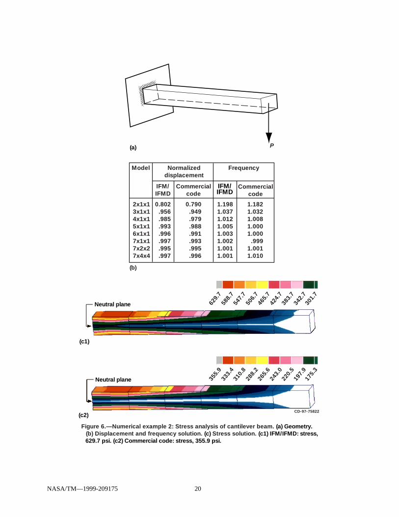
Numerical example 2: cantilever beam modeled by solid elements.—The cantilever beam shown in Fig. 6(a) is12 in. long, 1 in. deep, and 1 in. thick. It is made of steel with Young’s modulus of 30×106 psi and Poisson’s ratio of0.30 and is subjected to 10-lb load at its free end. The beam was modeled with hexahedral elements. For IFM/Analyzers the HEX2090 element was used. A 20-node CHEXA element was used for the commercial code. Thedisplacement, frequency, and stress solutions for different finite element models are given in Figs. 6(b) and (c). Themaximum displacement and fundamental frequency generated by IFM and the commercial code converged at aboutthe same rate. Difficulty was encountered for stress convergence. The stress patterns generated by IFM and the stiff-ness method looked similar. However, against a 720-psi beam solution, IFM converged to 630 psi, but the stiffnessmethod could produce only 356 psi for a six-element model.

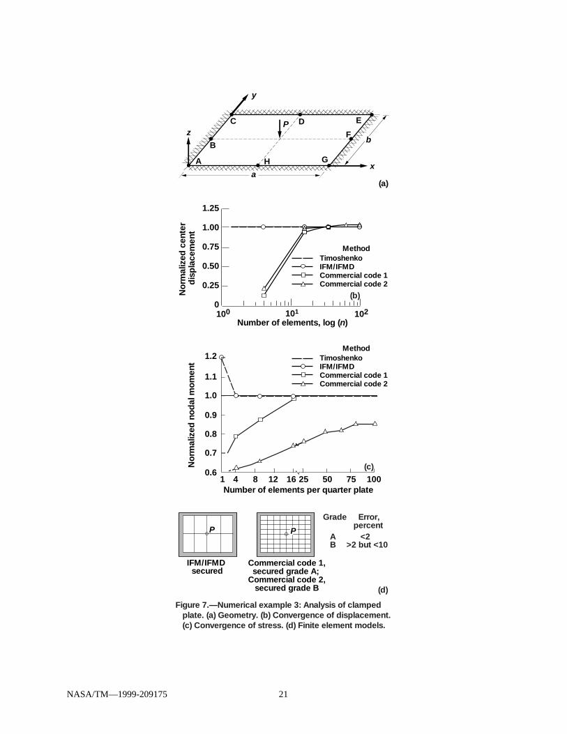
Numerical example 3: a plate flexure problem.—A rectangular clamped plate, shown in Fig. 7(a), subjected toa concentrated load of 1000 lb, was solved by using the PLB0409 element of IFM/Analyzers and by the CQUAD4element of a commercial code. The plate is made of steel with Young’s modulus of 30×106 psi and Poisson’s ratioof 0.30. Its dimensions (a, b, and thickness t, see Fig. 7) are 24, 12, and 0.25 in., respectively. Results normalizedwith respect to Timoshenko’s solutions (ref. 18) are depicted in Figs. 7(b) and (c). The central displacement ob-tained by IFM achieved an accuracy of 98.7 percent for a model with eight elements. For a coarser model with onlyfour elements the error was about 17.5 percent. The solution obtained by the commercial code required 64 elementsto achieve an accuracy of 98 percent. The performance of a second commercial code followed the pattern of the firstcode with some variation. For the bending moment convergence occurred with the PLB0409 element, using a modelwith four elements per quarter plate. For a model with one element per quarter plate the IFM solution exhibited a 20percent error. For the commercial code the bending moment exhibited an error of about 7 percent even for a finemodel with 16 elements per quarter plate.

For the three examples the integrated force method outperformed the stiffness method, overshadowing the sim-plicity at the element level.

DISCUSSION

The discussion is separated into the completeness of the theory, the quality of analytical predictions, and thenear-term research.

Completeness of Theory

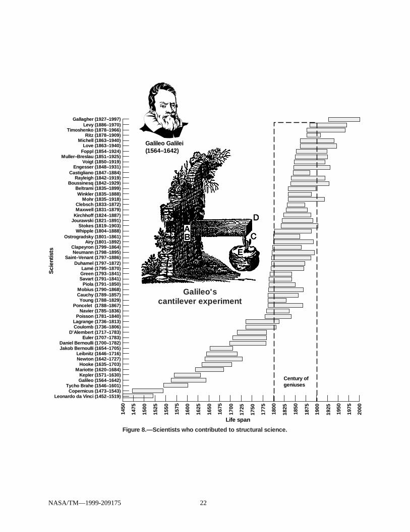
The theory of structures began before the birth of Newton in the notebooks of Leonardo da Vinci and throughGalileo Galilei’s studies on structures (ref. 1). The growth accelerated during the nineteenth century as the eminentscientists and engineers Cauchy, Navier, Saint-Venant, Castigliano, and others worked on different applications (seeFig. 8). It was commonly believed that all fundamental concepts of this four-century-old science were fully under-stood before the turn of the twentieth century. This belief was not correct. The traditional theory of compatibilitycamouflaged a deficiency described in this paper.

If the compatibility conditions were not required, the theory of (determinate) structures could be covered in afew undergraduate courses. Satisfying the compatibility conditions makes the theory a research topic practiced atdoctoral and postdoctoral levels around the world. Here we digress to speculate on the possible reasons for the tardyincorporation of the compatibility conditions into the theory of structures.

The compatibility conditions are more complex relationships than the equilibrium equations. However, it is notlikely that their complexity would have been an insurmountable obstacle for Cauchy, Saint-Venant, Navier, orMaxwell (see Fig. 8).

NASA/TM—1999-209175 13

Complacency could be another possible reason, but observed inconsistencies between different approaches tothe solution of indeterminate problems suggest that this could not have been the primary reason. For example, dis-placements are the unknowns in the displacement method, but redundants, instead of forces, became the unknownsin the traditional force method. Also, the displacement method could solve all three types of boundary value prob-lems in elasticity, but the Beltrami-Michell formulation could handle only stress boundary value problems. Theredundant force method in structures did not parallel the Beltrami-Michell formulation in elasticity. Even noviceresearchers would surely have noticed and questioned the lack of uniformity between the methods in elasticity andstructures.

Often an approximate solution was adequate to fulfill the need of an industry that may have had little interest inthe particular method used. Take, for example, the building and bridge industries, which require analysis of indeter-minate trusses, continuous beams, frames, and other structures. The redundant force method solved such problems.For plates and shells solutions obtained through the superposition technique served the industry well. Solving engi-neering problems not only became central to the work but also occupied most of the available time of competentresearchers, leaving little or no time for them to ponder or address the deficiencies and completion of the theory ofcompatibility. The engineering problem-solving aspect of structural mechanics was considered to be the most impor-tant. The dividends associated with solving industrial problems are, in our opinion, the primary reason behind theslow progress of the compatibility conditions. Complexity and complacency may be considered but secondaryreasons.

It is important to evaluate the completeness of the theory of structures as a science, as opposed to merely solv-ing industrial problems. The current acceptance of the stiffness solution by industry should not lead to neglect of thediscipline, which may have entered a developmental plateau. Research on compatibility can reinvigorate the struc-tures discipline and eventually provide a robust alternative formulation for solving industrial structures problems.

Quality of Analytical Prediction

The quality of analytical predictions can be directly controlled by imposing the requirement that the equilibriumequations and the compatibility conditions be simultaneously satisfied. The discretization error can be reducedthrough mesh refinement. The integrated force method adopts this approach and produces accurate solutions evenwhen the structure is modeled with a modest size of finite element mesh. Even though emphasis on and clevermanipulation of one of the two equation sets may appear to be adequate for the analysis of some problems, the reli-ability of the solution thus obtained cannot always be guaranteed. For example, the monotonically converged stiff-ness solution in Fig. 5 was erroneous.

Consider next a deficiency observed by Thodhunter (ref. 28) while he was scrutinizing Astronomer RoyalAiry’s attempt to analyze the stress in cantilever and simply supported beams. Airy formulated a potential functionto satisfy the equilibrium equations. He manipulated the equilibrium equations and the boundary conditions to gen-erate the solution for the examples. However, his results were incorrect because he neglected the compatibility com-pliance. Thodhunter (ref. 28) describes the situation:

Important Addition and Correction. The solution of the problems suggested in the last two Articleswere given—as has already been stated—on the authority of a paper by the late AstronomerRoyal, published in a report of the British Association. I now observe, however—when the print-ing of the articles and engraving of the Figures is already completed—that they cannot be acceptedas true solutions, inasmuch as they do not satisfy the general equations (164) of § 303 [note thatthe equations in question are the compatibility conditions]. It is perhaps as well that they should bepreserved as a warning to the students against the insidious and comparatively rare error of choos-ing a solution which satisfies completely all the boundary conditions, without satisfying the funda-mental condition of strain [note that the condition in question is the compatibility condition], andwhich is therefore of course not a solution at all.

The advice of Thodhunter should be followed to generate solutions by simultaneously satisfying all the equilibriumequations and all the compatibility conditions.

NASA/TM—1999-209175 14

Near-Term Research

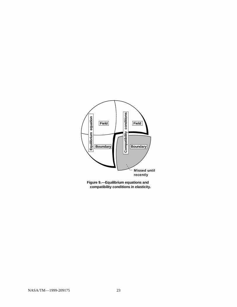
Equilibrium and compatibility constitute the two fundamental equations of the theory of structures, as depictedin the two halves of the pie diagram in Fig. 9. The immaturity in the compatibility conditions is represented by theshaded quarter. The theory of structures has been developed by using the information contained in three-quarters ofthe pie diagram. Using the additional quarter should improve the theory and the performance of the analysis meth-ods. Near-term research should address at least two issues: unification of the theory, and compliance of the boundarycompatibility conditions.

Unification of theory.—Using the compatibility conditions can lead to the unification of the theory of struc-tures, allowing free movement between different analysis variables as well as the various methods of structuralanalysis. In discrete element analysis we can move from displacement to stress through a set of algebraic equationsand vice versa. Likewise we should be able to move from force method to displacement method. For example, wecan move from the integrated force method to the dual integrated force method, both methods yielding identicalsolutions. Even though the IFM and IFMD produce identical solutions, each method has unique attributes. The pri-mal IFM is more suited to design optimization because this method generates closed-form sensitivities for stress,displacement, and frequency constraints (ref. 12). An analytical initial design to begin optimization iteration can beobtained by IFM (ref. 29). Singularity in optimization and behavior of constraints are elegantly treated by IFM(refs. 30 to 32). The dual IFMD is not as suitable as the primal IFM for design calculations. The governing matrixof IFMD is symmetrical. Therefore, IFMD can use solvers that have been obtained for the stiffness method. Thisapproach should be extended for continuum analysis, reducing any barrier between elasticity and structures. Forexample, the force method concept should be consistent between structures and elasticity (like the integrated forcemethod and the completed Beltrami-Michell formulation).

Satisfaction of boundary compatibility conditions.—The traditional solutions and other analysis methods mustbe checked for the compliance of the boundary compatibility conditions. Compliance of the BCC at the elementinterface in the stiffness-method-based finite element analysis should be reviewed. The stiffness elements, if neces-sary, should be modified for the compliance of the BCC.

CONCLUSIONS

The theory of structures has concealed a deficiency that has been present in the compatibility conditions sinceSaint-Venant’s strain formulation in 1860. We have researched and addressed these important conditions in struc-tures and elasticity.

Because of the compatibility deficiency the direct methods (integrated force method in structures and completedBeltrami-Michell formulation in elasticity) that bestow simultaneous emphasis on stress equilibrium and strain com-patibility were not available during the formative 1960’s. Despite the deficiency structural analysis has made mag-nificent progress through the stiffness method. However, in academia research into the stiffness method has entereda developmental plateau. Bringing back the method of forces can reinvigorate the discipline and provide a robustalternative formulation for solving industrial structural problems.

We can more precisely quantify the accuracy of predictions by comparing the force and stiffness method solu-tions and balance the monopoly that is currently biased toward the stiffness method. The new methods can bringvalue-added benefits in structural analysis, structural design, and structural testing.

REFERENCES

1. G. Galilei, Dialogues Concerning Two New Sciences, Northern University Press, Evanston, Illinois, 1950.2. P.H. Denke, A General Digital Computer Analysis of Statically Indeterminate Structures, NASA TN D–1666,

1962.3. J. Robinson, Automatic Selection of Redundancies in the Matrix Force Method: The Rank Technique,

Canadian Aeronautics J., 11, 9–12 (1965).

NASA/TM—1999-209175 15

4. A.E.H. Love, A Treatise on the Mathematical Theory of Elasticity, Fourth ed., Dover Publications, New York,1944, pp. 17, para. 1.

5. S.N. Patnaik, The Variational Energy Formulation for the Integrated Force Method, AIAA J., 24, 129–137 (Jan.1986).

6. I. Kaljevic, D.A. Hopkins, S. Saigal, and S.N. Patnaik, Completed Beltrami-Michell Formulation for AnalyzingMixed Boundary Value Problems in Elasticity, AIAA J., 34, 1, 143–148 (1996).

7. S.N. Patnaik, L. Berke, and R.H. Gallagher, Compatibility Conditions of Structural Mechanics for Finite Ele-ment Analysis, AIAA J., 29, 820–829 (May 1991).

8. S.N. Patnaik, L. Berke, and R.H. Gallagher, Integrated Force Method Versus Displacement Method for FiniteElement Analysis, Computers & Structures, 38, 4, 377–407 (1991).

9. S.N. Patnaik, R.M. Coroneos, and D.A. Hopkins, Dynamic Animation of Stress Modes via the Integrated ForceMethod of Structural Analysis, Int. J. Numer. Meth. Engrg., 40, 12, 2151–2169 (1997).

10. S.N. Patnaik, D.A. Hopkins, R.A. Aiello, and L. Berke, Improved Accuracy for Finite Element StructuralAnalysis via an Integrated Force Method, Computers & Structures, 45, 3, 521–542 (1992).

11. S.N. Patnaik, Integrated Force Method Versus the Standard Force Method, Computers & Structures, 22, 2,151–163 (1986).

12. S.N. Patnaik and R.H. Gallagher, Gradients of Behaviour Constraints and Reanalysis via the Integrated ForceMethod, Int. J. Numer. Meth. Engrg., 23, 2205–2212 (Dec. 1986).

13. O.C. Zienkiewicz, The Finite Element Method, McGraw-Hill, New York, 1977.14. R.H. Gallagher, Finite Element Analysis: Fundamentals, Prentice-Hall, Englewood Cliffs, New Jersey, 1975.15. J.H. Argyris and S. Kesley, Matrix Force Method of Structural Analysis With Applications to Aircraft Wings,

Wissenschaften Gessellschaft Luftfahrt, 1956, pp. 78–98.16. S.N. Patnaik and M.S. Nagaraj, Analysis of Continuum by the Integrated Force Method, Computers & Struc-

tures, 26, 6, 899–905 (1987).17. K. Vijayakumar, A.V. Krishna Murty, and S.N. Patnaik, A Basis for the Analysis of Solid Continua Using the

Integrated Force Method, AIAA J., 26, 628–629 (May 1988).18. S. Timoshenko and S. Woinowsky-Krieger, Theory of Plates and Shells, McGraw-Hill, New York, 1959.19. I.S. Sokolnikoff, Mathematical Theory of Elasticity, Second ed., McGraw-Hill, New York, 1956.20. K. Washizu, Variational Methods in Elasticity and Plasticity, Second ed., Pergamon Press, New York, 1975.21. J.S. Przemieniecki, Theory of Matrix Structural Analysis, McGraw-Hill, New York, 1968.22. S.N. Patnaik and H.G. Satish, Analysis of Continuum Using the Boundary Compatibility Conditions of Inte-

grated Force Method, Computers & Structures, 34, 2, 287–295 (1990).23. S.N. Patnaik, A.S. Gendy, L. Berke, and D.A. Hopkins, Modified Fully Utilized Design Method (MFUD) for

Stress and Displacement Constraints, Int. J. Num. Meth. Engrg., 41, 7, 1171–1194 (1998).24. S.N. Patnaik, D.A. Hopkins, and R. Coroneos, Structural Optimization With Approximate Sensitivities, Com-

puters & Structures, 58, 407–418 (1996). (Also NASA TM–4553.)25. I. Kaljevic, S.N. Patnaik, and D.A. Hopkins, Development of Finite Elements for Two-Dimensional Structural

Analysis Using the Integrated Force Method, Computers & Structures, 59, 4, 691–706 (1996).26. I. Kaljevic, S.N. Patnaik, and D.A. Hopkins, Three-Dimensional Structural Analysis by the Integrated Force

Method, Computers & Structures, 58, 5, 869–886 (1996).27. R.L. Spilker, S.M. Maskeri, and E. Kania, Plane Isoparametric Hybrid-Stress Elements: Invariance and Optimal

Sampling, Int. J. Numer. Meth. Engrg., 17, 10, 1469–1496 (1981).28. I. Thodhunter, A History of the Theory of Elasticity and of the Strength of Materials, From Galilei to the

Present Time, University Press, K. Pearson, ed., Cambridge, England, pp. 1886–1893.29. S.N. Patnaik, Analytical Initial Design for Structural Optimization via the Integrated Force Method, Computers

& Structures, 33, 7, 265–268 (1989).30. S.N. Patnaik, J.D. Guptill, and L. Berke, Singularity in Structural Optimization, Int. J. Numer. Meth. Engrg., 36,

6, 931–944 (1993).31. S.N. Patnaik and P. Dayaratnam, Behavior and Design of Pin-Connected Structures, Int. J. Numer. Meth.

Engrg., 12, 579–595 (1972).32. P. Dayaratnam and S.N. Patnaik, Feasibility of Full Stress Design, AIAA J., 7, 773–774 (1969).

NASA/TM—1999-209175 16

TABLE I.—METHODS OF STRUCTURAL MECHANICS AND ASSOCIATED VARIATIONALFUNCTIONALS

Method Method Primary variable Variationalnumber Elasticity Structures Elasticity Structure functional

1 CompletedBeltrami-Michellformulation

Integrated forcemethod

Stress Force IFM variationalfunctional

2 Airy formulation Redundant forcemethod

Stress function Redundant Complementaryenergy

3 Navier formulation Stiffness methodDisplacement Deflection Potential energy4 Hybrid method Reissner method Stress and

displacementForce and deflection Reissner functional

5 Total formulation Washizu method Stress, strain, anddisplacement

Force, deformation,and deflection

Washizu functional

Figure 1.—Compatibility barrier to extending force method for indeterminate structures.

Determinate structures

[Equilibrium] {F} = {P}Equilibrium

CompatibilityP

Initial deformation

Indeterminate structures

Stiffness method(popular to extent of monopoly)

No Yes

Could not be extendedIntegrated force method

Redundant force method(disappeared)

Co

mp

atib

ility

bar

rier Stif

fnes

s met

hod

Navier

(178

5–18

36)

Redundant force method

Castigliano (1847–1884)

Method of forces(identical to IFM)

Tra

nsfo

rmat

ion

YesNo

Tra

nsfo

rmat

ion

2nd

hal

f o

f20

th c

entu

ry

{F} =

NASA/TM—1999-209175 17

(a)

R2

R3

z

yx

ey

ex

2b

2a

P

R1

w

R4

,

A

(b)

(c) (d)

Figure 2.—IFM solution to Navier's table problem. (a) Indeterminate table problem. (b) Average displacement along z-axis. (c) Average tilt about x-axis. (d) Average tilt about y-axis.

R4

R3

R1 R2

R4 R3

R1 R2

ux

R4 R3

R1 R2

uy

NASA/TM—1999-209175 18

(a)

(b)

Figure 3.—Composite circular plate subjected to uniform load q and temperature differential Dt. (a) Side view of plate. (b) Planform of plate.

Dt Dt

II I II

q

a

b

u

r

Thermally (Dt) loaded outer plate (II)

Mechnically (q) loaded inner plate

NASA/TM—1999-209175 19

Figure 4.—Boundary compatibility compliance for two-element model.

5

1

4

2

23

1

(a1)

1 2 3 n• • •

(a2)

a = 24 in.

P/2

P/2

A

b = 2 in.

y

x

0.25 in.

y

1.0

0.9

0.8

0.7

0.6

0.51 3 6 9 12 15 18 21 24

0.914

IFM/Analyzers (QUAD0405)Commercial code (CQUAD4)

Number of elements in model, n

No

rmal

ized

tip

dis

pla

cem

ent

1.1

1.002

(b)

Figure 5.—Numerical example 1: Analysis of cantilever beam. (a1) Geometry and boundary conditions. (a2) Finite element model. (b) Convergence of cantilever beam tip displacement.

NASA/TM—1999-209175 20

2x1x13x1x14x1x15x1x16x1x17x1x17x2x27x4x4

0.802.956.985.993.996.997.995.997

0.790.949.979.988.991.993.995.996

1.1981.0371.0121.0051.0031.0021.0011.001

1.1821.0321.0081.0001.000 .9991.0011.010

Model Normalizeddisplacement

Frequency

IFM/IFMD

IFM/IFMD

Commercialcode

Commercialcode

P

(c2)

Neutral plane

(c1)

(b)

(a)

Neutral plane

355.

933

3.4

310.

828

8.2

265.

624

3.0

220.

519

7.9

175.

3

629.

758

8.7

547.

750

6.7

465.

742

4.7

383.

734

2.7

301.

7

CD-97-75822

Figure 6.—Numerical example 2: Stress analysis of cantilever beam. (a) Geometry. (b) Displacement and frequency solution. (c) Stress solution. (c1) IFM/IFMD: stress, 629.7 psi. (c2) Commercial code: stress, 355.9 psi.

NASA/TM—1999-209175 21

(a)

P

y

b

x

z

a

B

A H

C D E

F

G

1.2

1.1

1.0

0.9

0.8

0.7

0.61 4 8 12 16 25 50 75 100Number of elements per quarter plate

No

rmal

ized

no

dal

mo

men

t

IFM/IFMD secured

Commercial code 1,secured grade A;

Commercial code 2,secured grade B

P PP

(d)

(b)

(c)

1.25

1.00

0.75

0.50

0.25

0100 101 102

Number of elements, log (n)

No

rmal

ized

cen

ter

dis

pla

cem

ent

TimoshenkoIFM/IFMD Commercial code 1Commercial code 2

Method

TimoshenkoIFM/IFMD Commercial code 1Commercial code 2

Method

Grade Error, percent

A <2 B >2 but <10

Figure 7.—Numerical example 3: Analysis of clamped plate. (a) Geometry. (b) Convergence of displacement. (c) Convergence of stress. (d) Finite element models.

NASA/TM—1999-209175 22

1450

1475

1500

1525

1575

1600

1625

1650

1675

1700

1725

1550

1750

1775

1825

1800

1850

1875

1925

1900

1950

1975

2000

Century ofgeniuses

Life span

Sci

entis

ts

Galileo'scantilever experiment

Figure 8.—Scientists who contributed to structural science.

Galileo Galilei(1564–1642)

Ritz (1878–1909)Timoshenko (1878–1966)

Michell (1863–1940)Love (1863–1940)

Foppl (1854–1924)Muller–Breslau (1851–1925)

Voigt (1850–1919)Engesser (1848–1931)

Castigliano (1847–1884)Rayleigh (1842–1919)

Boussinesq (1842–1929)Beltrami (1835–1899)Winkler (1835–1888)

Mohr (1835–1918)Clebsch (1833–1872)Maxwell (1831–1879)

Kirchhoff (1824–1887)Jourawski (1821–1891)

Stokes (1819–1903)Whipple (1804–1888)

Ostrogradsky (1801–1861)Airy (1801–1892)

Clapeyron (1799–1864)Neumann (1798–1895)

Saint–Venant (1797–1886)Duhamel (1797–1872)

Lamé (1795–1870)Green (1793–1841)Savart (1791–1841)

Piola (1791–1850)Mobius (1790–1868)Cauchy (1789–1857)Young (1788–1829)

Poncelet (1788–1867)Navier (1785–1836)

Poisson (1781–1840)Lagrange (1736–1813)Coulomb (1736–1806)

D'Alembert (1717–1783)Euler (1707–1783)

Daniel Bernoulli (1700–1782)Jakob Bernoulli (1654–1705)

Leibnitz (1646–1716)Newton (1642–1727)Hooke (1635–1703)

Mariotte (1620–1684)Kepler (1571–1630)Galileo (1564–1642)

Tycho Brahe (1546–1601)Copernicus (1473–1543)

Leonardo da Vinci (1452–1519)

Levy (1886–1970)Gallagher (1927–1997)

NASA/TM—1999-209175 23

Figure 9.—Equilibrium equations and compatibility conditions in elasticity.

recentlyMissed until

Eq

uilib

rium

eq

uatio

n

Field

Boundary

Field

Boundary

Co

mp

atib

ility

co

nditi

ons

This publication is available from the NASA Center for AeroSpace Information, (301) 621–0390.

REPORT DOCUMENTATION PAGE

2. REPORT DATE

19. SECURITY CLASSIFICATION OF ABSTRACT

18. SECURITY CLASSIFICATION OF THIS PAGE

Public reporting burden for this collection of information is estimated to average 1 hour per response, including the time for reviewing instructions, searching existing data sources,gathering and maintaining the data needed, and completing and reviewing the collection of information. Send comments regarding this burden estimate or any other aspect of thiscollection of information, including suggestions for reducing this burden, to Washington Headquarters Services, Directorate for Information Operations and Reports, 1215 JeffersonDavis Highway, Suite 1204, Arlington, VA 22202-4302, and to the Office of Management and Budget, Paperwork Reduction Project (0704-0188), Washington, DC 20503.

NSN 7540-01-280-5500 Standard Form 298 (Rev. 2-89)Prescribed by ANSI Std. Z39-18298-102

Form Approved

OMB No. 0704-0188

12b. DISTRIBUTION CODE

8. PERFORMING ORGANIZATION REPORT NUMBER

5. FUNDING NUMBERS

3. REPORT TYPE AND DATES COVERED

4. TITLE AND SUBTITLE

6. AUTHOR(S)

7. PERFORMING ORGANIZATION NAME(S) AND ADDRESS(ES)

11. SUPPLEMENTARY NOTES

12a. DISTRIBUTION/AVAILABILITY STATEMENT

13. ABSTRACT (Maximum 200 words)

14. SUBJECT TERMS

17. SECURITY CLASSIFICATION OF REPORT

16. PRICE CODE

15. NUMBER OF PAGES

20. LIMITATION OF ABSTRACT

Unclassified Unclassified

Technical Memorandum

Unclassified

National Aeronautics and Space AdministrationJohn H. Glenn Research Center at Lewis FieldCleveland, Ohio 44135–3191

1. AGENCY USE ONLY (Leave blank)

10. SPONSORING/MONITORING AGENCY REPORT NUMBER

9. SPONSORING/MONITORING AGENCY NAME(S) AND ADDRESS(ES)

National Aeronautics and Space AdministrationWashington, DC 20546–0001

November 1999

NASA TM—1999-209175

E–11682

WU–523–22–13–00

29

A03

Compatibility Conditions of Structural Mechanics

Surya N. Patnaik, Rula M. Coroneos, and Dale A. Hopkins

Compatibility conditions; Finite element method; Integrated force method; Structures;Elasticity

Unclassified -UnlimitedSubject Category: 39 Distribution: Standard

Surya N. Patnaik, Ohio Aerospace Institute, 22800 Cedar Point Road, Cleveland, Ohio 44142; Rula M. Coroneosand Dale A. Hopkins, NASA Glenn Research Center. Responsible person, Surya N. Patnaik, organization code 5930,(216) 433–5916.

The theory of elasticity has camouflaged a deficiency in the compatibility formulation since 1860. In structures the adhoc compatibility conditions through virtual “cuts” and closing “gaps” are not parallel to the strain formulation inelasticity. This deficiency in the compatibility conditions has prevented the development of a direct stress determinationmethod in structures and in elasticity. We have addressed this deficiency and attempted to unify the theory of compatibil-ity. This work has led to the development of the integrated force method for structures and the completed Beltrami-Michell formulation for elasticity. The improved accuracy observed in the solution of numerical examples by the inte-grated force method can be attributed to the compliance of the compatibility conditions. Using the compatibility condi-tions allows mapping of variables and facile movement among different structural analysis formulations. This paperreviews and illustrates the requirement of compatibility in structures and in elasticity. It also describes the generation ofthe conditions and quantifies the benefits of their use. The traditional analysis methods and available solutions (whichhave been obtained bypassing the missed conditions) should be verified for compliance of the compatibility conditions.