Embed Size (px)
Citation preview
Compartmentalizing State Machine Replication
by
Michael Whittaker
A dissertation submitted in partial satisfaction of the
requirements for the degree of
Doctor of Philosophy
in
Computer Science
in the
Graduate Division
of the
University of California, Berkeley
Committee in charge:
Professor Joseph Hellerstein, ChairAssistant Professor Natacha Crooks
Assistant Professor Barna SahaProfessor Ion Stoica
Summer 2021

Compartmentalizing State Machine Replication
Copyright 2021by
Michael Whittaker

1
Abstract
Compartmentalizing State Machine Replication
by
Michael Whittaker
Doctor of Philosophy in Computer Science
University of California, Berkeley
Professor Joseph Hellerstein, Chair
State machine replication is at the heart of almost every strongly consistent distributedsystem. In this thesis, we introduce a novel technique called compartmentalization that in-volves decoupling a protocol into its simplest components and then scaling each componentindependently. Compartmentalization is simple yet effective. It can be used to increase thethroughput of a protocol, to simplify an exiting protocol, or to design new functionalityfor a protocol. In this thesis specifically, we apply compartmentalization to state machinereplication protocols in a number of different ways. We compartmentalize MultiPaxos andincrease its throughput by over an order of magnitude. We then compartmentalize a familyof complex state machine protocols called generalized multi-leader protocols. The compart-mentalization simplifies the protocols and brings clarity to a family of protocols that werepreviously extremely difficult to understand. Finally, we use compartmentalization to de-sign a new reconfiguration protocol based on Vertical Paxos that state machine replicationprotocols can use to replace failed machines with new machines without any downtime.

i
To my friends and family

ii
Contents
Contents ii
List of Figures iv
List of Tables ix
1 Introduction 1
2 Background 42.1 System Model . . . . . . . . . . . . . . . . . . . . . . . . . . . . . . . . . . . 42.2 Paxos . . . . . . . . . . . . . . . . . . . . . . . . . . . . . . . . . . . . . . . 42.3 MultiPaxos . . . . . . . . . . . . . . . . . . . . . . . . . . . . . . . . . . . . 82.4 Flexible Paxos . . . . . . . . . . . . . . . . . . . . . . . . . . . . . . . . . . . 9
3 Compartmentalization 103.1 MultiPaxos Does Not Scale? . . . . . . . . . . . . . . . . . . . . . . . . . . . 113.2 Compartmentalizing MultiPaxos . . . . . . . . . . . . . . . . . . . . . . . . . 123.3 Batching . . . . . . . . . . . . . . . . . . . . . . . . . . . . . . . . . . . . . . 263.4 Mencius . . . . . . . . . . . . . . . . . . . . . . . . . . . . . . . . . . . . . . 303.5 S-Paxos . . . . . . . . . . . . . . . . . . . . . . . . . . . . . . . . . . . . . . 333.6 Evaluation . . . . . . . . . . . . . . . . . . . . . . . . . . . . . . . . . . . . . 353.7 Related Work . . . . . . . . . . . . . . . . . . . . . . . . . . . . . . . . . . . 44
4 Quoracle 484.1 Definitions . . . . . . . . . . . . . . . . . . . . . . . . . . . . . . . . . . . . . 494.2 Practical Refinements in Quoracle . . . . . . . . . . . . . . . . . . . . . . . . 514.3 Case Study . . . . . . . . . . . . . . . . . . . . . . . . . . . . . . . . . . . . 584.4 Lessons Learned . . . . . . . . . . . . . . . . . . . . . . . . . . . . . . . . . . 60
5 Bipartisan Paxos 625.1 Conflict Graphs . . . . . . . . . . . . . . . . . . . . . . . . . . . . . . . . . . 635.2 Simple BPaxos . . . . . . . . . . . . . . . . . . . . . . . . . . . . . . . . . . 685.3 Fast Paxos . . . . . . . . . . . . . . . . . . . . . . . . . . . . . . . . . . . . . 77

iii
5.4 Fast BPaxos . . . . . . . . . . . . . . . . . . . . . . . . . . . . . . . . . . . . 815.5 Tension Avoidance . . . . . . . . . . . . . . . . . . . . . . . . . . . . . . . . 855.6 Tension Resolution . . . . . . . . . . . . . . . . . . . . . . . . . . . . . . . . 905.7 Related Work . . . . . . . . . . . . . . . . . . . . . . . . . . . . . . . . . . . 955.8 Conclusion . . . . . . . . . . . . . . . . . . . . . . . . . . . . . . . . . . . . . 97
6 Matchmaker Paxos 1016.1 Matchmaker Paxos . . . . . . . . . . . . . . . . . . . . . . . . . . . . . . . . 1036.2 Matchmaker MultiPaxos . . . . . . . . . . . . . . . . . . . . . . . . . . . . . 1136.3 Reconfiguring Matchmakers . . . . . . . . . . . . . . . . . . . . . . . . . . . 1186.4 Theoretical Insights . . . . . . . . . . . . . . . . . . . . . . . . . . . . . . . . 1216.5 Evaluation . . . . . . . . . . . . . . . . . . . . . . . . . . . . . . . . . . . . . 1286.6 Related Work . . . . . . . . . . . . . . . . . . . . . . . . . . . . . . . . . . . 133
7 Conclusion and Lessons Learned 137
Bibliography 139

iv
List of Figures
2.1 An example execution of Paxos (f = 1). . . . . . . . . . . . . . . . . . . . . . . 52.2 At time t = 0, no state machine commands are chosen. At time t = 1 command
x is chosen in slot 0. At times t = 2 and t = 3, commands z and y are chosen inslots 2 and 1. Executed commands are shaded green. Note that all state machinesexecute the commands x, y, z in log order. . . . . . . . . . . . . . . . . . . . . 8
2.3 An example execution of MultiPaxos (f = 1). The leader is adorned with a crown. 9
3.1 An example execution of Compartmentalized MultiPaxos with three proxy leaders(f = 1). Throughout the chapter, nodes and messages that were not present inprevious iterations of the protocol are highlighted in green. . . . . . . . . . . . 13
3.2 An execution of Compartmentalized MultiPaxos with a 2 × 3 grid of acceptors(f = 1). The two read quorums—{a1, a2, a3} and {a4, a5, a6}—are shown in solidred rectangles. The three write quorums—{a1, a4}, {a2, a5}, and {a3, a6}—areshown in dashed blue rectangles. . . . . . . . . . . . . . . . . . . . . . . . . . . 16
3.3 An example execution of Compartmentalized MultiPaxos with three replicas asopposed to the minimum required two (f = 1). . . . . . . . . . . . . . . . . . . 17
3.4 An example execution of Compartmentalized MultiPaxos’ read and write path(f = 1) with a 2×2 acceptor grid. The write path is shown using solid blue lines.The read path is shown using red dashed lines. . . . . . . . . . . . . . . . . . . 19
3.5 . . . . . . . . . . . . . . . . . . . . . . . . . . . . . . . . . . . . . . . . . . . . . 203.6 An execution that is not linearizable . . . . . . . . . . . . . . . . . . . . . . . . 213.7 A history, Hpending, with a pending invocation . . . . . . . . . . . . . . . . . . . 213.8 Hwwr | c1 . . . . . . . . . . . . . . . . . . . . . . . . . . . . . . . . . . . . . . . . 223.9 Hwrw . . . . . . . . . . . . . . . . . . . . . . . . . . . . . . . . . . . . . . . . . . 223.10 Swrw . . . . . . . . . . . . . . . . . . . . . . . . . . . . . . . . . . . . . . . . . . 233.11 A motivating example of history extension . . . . . . . . . . . . . . . . . . . . . 233.12 An example history G. Responses are not shown, as they are not important for
this example. . . . . . . . . . . . . . . . . . . . . . . . . . . . . . . . . . . . . . 243.13 A linearization SG of the history in G Figure 3.12 . . . . . . . . . . . . . . . . . 24

v
3.14 An example execution of Compartmentalized MultiPaxos with batching (f = 1).Messages that contain a batch of commands, rather than a single command, aredrawn thicker. Note how replica r2 has to send multiple messages after executinga batch of commands. . . . . . . . . . . . . . . . . . . . . . . . . . . . . . . . . 27
3.15 An example execution of Compartmentalized MultiPaxos with batchers (f = 1). 283.16 An example execution of Compartmentalized MultiPaxos with unbatchers (f =
1). . . . . . . . . . . . . . . . . . . . . . . . . . . . . . . . . . . . . . . . . . . . 293.17 A Mencius log round robin partitioned among three leaders. . . . . . . . . . . . 303.18 An example of using noops to deal with a slow leader. Leader l3 is slower than
leaders l1 and l2, so the log has holes in l3’s slots. l3 fills its holes with noops toallow commands in the log to be executed. . . . . . . . . . . . . . . . . . . . . 31
3.19 An example execution of Mencius. . . . . . . . . . . . . . . . . . . . . . . . . . . 313.20 An example execution of decoupled Mencius. Note that every proposer is a leader. 323.21 An execution of Mencius with proxy leaders, acceptor grids, and an increased
number of replicas. . . . . . . . . . . . . . . . . . . . . . . . . . . . . . . . . . 333.22 An example execution of S-Paxos. Messages that include client commands (as
opposed to ids) are bolded. . . . . . . . . . . . . . . . . . . . . . . . . . . . . . 343.23 An example execution of decoupled S-Paxos. Messages that include client com-
mands (as opposed to ids) are bolded. Note that the MultiPaxos leader does notsend or receive any messages that include a command, only messages that includecommand ids. . . . . . . . . . . . . . . . . . . . . . . . . . . . . . . . . . . . . 35
3.24 An example execution of S-Paxos with stabilizer grids, proxy leaders, acceptorgrids, and an increased number of replicas. Messages that include client com-mands (as opposed to ids) are bolded. . . . . . . . . . . . . . . . . . . . . . . . 36
3.25 The latency and throughput of MultiPaxos, Compartmentalized MultiPaxos, andan unreplicated state machine. . . . . . . . . . . . . . . . . . . . . . . . . . . . 37
3.26 The latency and throughput of Compartmentalized MultiPaxos and an unrepli-cated state machine without batching and with larger value sizes. . . . . . . . . 39
3.27 An ablation study. Standard deviations are shown using error bars. . . . . . . . 393.28 Peak throughput vs the number of replicas . . . . . . . . . . . . . . . . . . . . 403.29 Analytical throughput vs the number of replicas. . . . . . . . . . . . . . . . . . 423.30 Peak throughput vs the number of replicas . . . . . . . . . . . . . . . . . . . . 433.31 The effect of skew on Compartmentalized MultiPaxos and CRAQ. . . . . . . . 44
4.1 The 2 by 3 grid quorum system Q2×3. . . . . . . . . . . . . . . . . . . . . . . . . 504.2 Quorum systems, capacity, and fault tolerance. . . . . . . . . . . . . . . . . . . 524.3 Heterogeneous nodes with different capacities. . . . . . . . . . . . . . . . . . . . 534.4 A distribution of read fractions. . . . . . . . . . . . . . . . . . . . . . . . . . . . 544.5 Strategy capacities with respect to read fraction . . . . . . . . . . . . . . . . . . 544.6 0-resilient and 1-resilient strategies. . . . . . . . . . . . . . . . . . . . . . . . . . 564.7 Finding a latency-optimal strategy with capacity and network load constraints. 574.8 Searching the space of quorum systems. . . . . . . . . . . . . . . . . . . . . . . 58

vi
4.9 Nodes and workload distribution. . . . . . . . . . . . . . . . . . . . . . . . . . . 584.10 The read quorums of the staggered grid and paths quorum systems. The optimal
set of complementary write quorums is chosen automatically. . . . . . . . . . . 594.11 Quorum systems and their capacities. . . . . . . . . . . . . . . . . . . . . . . . . 594.12 Searching for a load-optimal quorum system. . . . . . . . . . . . . . . . . . . . . 594.13 Latencies with a capacity constraint. . . . . . . . . . . . . . . . . . . . . . . . . 604.14 A stacked histogram of the throughput of a simple majority quorum system with
a naive uniform strategy. Write quorums are in blue, and read quorums are in red. 614.15 A stacked histogram of the throughput of the quorum system found by our heuris-
tic search (i.e., the quorum system with read quorums (c+ bd)(a+ e)). . . . . . 61
5.1 If two commands commute, replicas can safely execute them in either order. . . 645.2 A log and corresponding conflict graph. . . . . . . . . . . . . . . . . . . . . . . . 655.3 In subfigures (a) - (e), we see a conflict graph constructed over time. The most
recently chosen vertex is drawn in red. The executed commands are shadedgreen. (a) The command a=b is chosen in vertex v0 without any dependencies.The command is executed immediately. (b) The command a=2 is chosen in vertexv1 with a dependency on v0. The command is executed immediately. (c) Thecommand b=a is chosen in vertex v3 with dependencies on v0, v1, v2, and v4.No commands have been chosen in v2 and v4 yet, so v3 cannot be executed.(d) The command b=1 is chosen in vertex v2 with a dependency on v0. Thecommand is executed immediately. (e) The command a=3 is chosen in vertex v4with dependencies on v0, v1, and v3. Now v3 and v4 are executed. In subfigures(f) - (j), we see an analogous execution for a log. . . . . . . . . . . . . . . . . . 66
5.4 An example execution of Simple BPaxos (f = 1). . . . . . . . . . . . . . . . . . 685.5 In subfigures (a) – (e), we see the execution of a dependency service node di. (a)
di receives command w in vertex vw. di adds this vertex to its conflict graph andbecause there are no other vertices, it returns the dependencies deps(vw) = ∅. (b)di receives command x in vertex vx. di adds this vertex to its conflict graph. xconflicts with w, so di adds an edge from vx to vw and returns the dependenciesdeps(vx) = {vw}. (c) di receives command y in vertex vy. di adds this vertex toits conflict graph. y conflicts with w and x, so di adds an edge from vy to vw andfrom vy to vx. It returns the dependencies deps(vy) = {vw, vx}. (d) di receivescommand z in vertex vz. di adds this vertex to its conflict graph. z conflictswith w and x, so di adds an edge from vz to vw and from vz to vx. It returns thedependencies deps(vz) = {vw, vx}. (e) di receives command x in vertex vx. di’sgraph already contains vertex vx, so di returns the dependencies deps(vx) = {vw}and does not modify its graph. . . . . . . . . . . . . . . . . . . . . . . . . . . . 70
5.6 An example execution of Simple BPaxos (f = 1). . . . . . . . . . . . . . . . . . 725.7 An example execution of Simple BPaxos recovery (f = 1). . . . . . . . . . . . . 735.8 An example of dependency compaction . . . . . . . . . . . . . . . . . . . . . . . 76

vii
5.9 Example executions of Fast Paxos (f = 2). The leader of round 0 is adorned witha crown. Client requests are drawn in red. Phase 1 messages are drawn in blue.Phase 2 messages are drawn in green. . . . . . . . . . . . . . . . . . . . . . . . 79
5.10 An example execution of Fast BPaxos (f = 1). The four network delays aredrawn in red. . . . . . . . . . . . . . . . . . . . . . . . . . . . . . . . . . . . . . 82
5.11 A Fast BPaxos bug (f = 2). Conflicting commands x and y are executed indifferent orders by different replicas. . . . . . . . . . . . . . . . . . . . . . . . . 84
5.12 An example execution of Unanimous BPaxos (f = 2) with the Basic EPaxosoptimization. The messages introduced by the optimization are drawn in red. . 88
5.13 A non-exhaustive taxonomy of state machine replication protocols. The gener-alized multi-leader protocols that we discuss in this chapter are shaded green.. . . . . . . . . . . . . . . . . . . . . . . . . . . . . . . . . . . . . . . . . . . . . 96
6.1 Matchmaker Paxos (f = 1). . . . . . . . . . . . . . . . . . . . . . . . . . . . . . 1046.2 A matchmaker’s log over time. (a) Initially, the matchmaker’s log is empty. (b)
Then, the matchmaker receives MatchA〈0, C0〉. It inserts C0 in log entry 0and returns MatchB〈0, ∅〉 since the log does not contain any configuration inany round less than 0. (c) The matchmaker then receives MatchA〈2, C2〉. Itinserts C2 in log entry 2 and returns MatchB〈2, {(0, C0)}〉. (d) It then receivesMatchA〈3, C3〉, inserts C3 in log entry 3, and returns MatchB〈3, {(0, C0), (2, C2)}〉.At this point, if the matchmaker were to receive MatchA〈1, C1〉, it would ignoreit. . . . . . . . . . . . . . . . . . . . . . . . . . . . . . . . . . . . . . . . . . . . 105
6.3 A leader’s knowledge of the log after Phase 1. . . . . . . . . . . . . . . . . . . . 1136.4 An example Matchmaker MultiPaxos reconfiguration without Phase 1 bypassing.
The leader p1 reconfigures from the acceptors a1, a2, a3 to the acceptors b1, b2,b3. Client commands are drawn as gray dashed lines. Note that every subfigureshows one phase of a reconfiguration using solid colored lines, but the dashedlines show the complete execution of a client request that runs concurrently withthe reconfiguration. For simplicity, we assume that every proposer also serves asa replica. . . . . . . . . . . . . . . . . . . . . . . . . . . . . . . . . . . . . . . . 115
6.5 An example of merging three matchmaker logs (L0, L1, and L2) during a match-maker reconfiguration. Garbage collected log entries are shown in red. . . . . . 119
6.6 A MultiPaxos log during reconfiguration (α = 4). . . . . . . . . . . . . . . . . . 1216.7 Matchmaker MultiPaxos’ latency and throughput (f = 1). Median latency is
shown using solid lines, while the 95% latency is shown as a shaded region abovethe median latency. The vertical black lines show reconfigurations. The verticaldashed red line shows an acceptor failure. . . . . . . . . . . . . . . . . . . . . . 129
6.8 The latency and throughput of MultiPaxos with horizontal reconfiguration (f =1). . . . . . . . . . . . . . . . . . . . . . . . . . . . . . . . . . . . . . . . . . . . 130
6.9 Violin plots of Figure 6.7 latency and throughput during the first 10 seconds andbetween 10 and 20 seconds. . . . . . . . . . . . . . . . . . . . . . . . . . . . . . 131

viii
6.10 Violin plots of Figure 6.8 latency and throughput during the first 10 seconds andbetween 10 and 20 seconds. . . . . . . . . . . . . . . . . . . . . . . . . . . . . . 132
6.11 Matchmaker MultiPaxos’ latency and throughput (f = 1). The dashed red linedenotes a leader failure. . . . . . . . . . . . . . . . . . . . . . . . . . . . . . . . 134
6.12 The latency and throughput of Horizontal MultiPaxos with f = 1. . . . . . . . 1356.13 The latency and throughput of Matchmaker MultiPaxos (f = 1). The dotted
blue, dashed red, and vertical black lines show matchmaker reconfigurations, amatchmaker failure, and an acceptor reconfiguration respectively. . . . . . . . . 136
ix
List of Tables
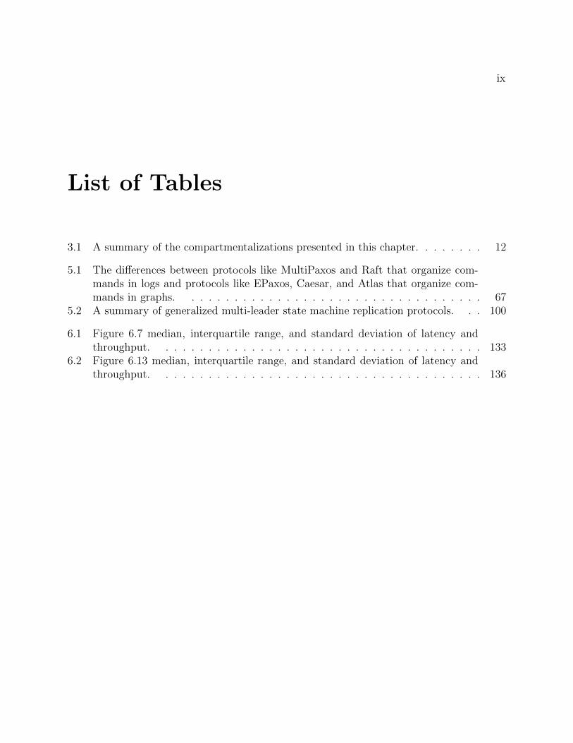
3.1 A summary of the compartmentalizations presented in this chapter. . . . . . . . 12
5.1 The differences between protocols like MultiPaxos and Raft that organize com-mands in logs and protocols like EPaxos, Caesar, and Atlas that organize com-mands in graphs. . . . . . . . . . . . . . . . . . . . . . . . . . . . . . . . . . . 67
5.2 A summary of generalized multi-leader state machine replication protocols. . . 100
6.1 Figure 6.7 median, interquartile range, and standard deviation of latency andthroughput. . . . . . . . . . . . . . . . . . . . . . . . . . . . . . . . . . . . . . 133
6.2 Figure 6.13 median, interquartile range, and standard deviation of latency andthroughput. . . . . . . . . . . . . . . . . . . . . . . . . . . . . . . . . . . . . . 136

x
Acknowledgments
I am immensely grateful to Joseph Hellerstein, my advisor. Joe, you are one of the biggestreasons I came to Berkeley, and I am so happy I did. You know so much about so much,and you grok things so quickly. You have always been in my corner and have always hadmy back. You put your full faith and confidence in me and motivated me throughout myPhD. You were a mentor and a friend to whom I could always turn. From the bottom of myheart, thank you Joe!
I was so fortunate to work closely with Ion Stoica. Ion, you have always been so sharp,always able to predict what I’m going to say before I say it. I’ve benefited tremendously fromyour experience and insights. From paper advice to career advice to life advice, I alwaysrelish the opportunity to learn from you. Thank you Ion!
Natacha Crooks, we missed each other at Cornell and overlapped for only a year duringa quarantine at Berkeley. I really wish we had more overlap because collaborating with youhas been amazing. You are such a friendly and uplifting mentor, and I always felt like youwere looking out for me. I hope we cross paths again in the future.
Barna Saha, thank you for serving on my qual and dissertation committee. Your feedbackis always insightful.
Neil Giridharan, we’ve been working together since the day I started working on consen-sus. You have been an absolute dream of a collaborator, and I can’t imagine doing any ofthe research without you. Three years ago, we used to talk about vanilla Paxos, and nowyou’re inventing Byzantine consensus protocols with the world’s leading experts. I am soproud of what you have already achieved and will continue to achieve, and I wish you thebest of luck in grad school!
Heidi Howard, you are in my opinion the world’s leading expert on consensus and statemachine replication. Heidi, your effect on me started before we even met. Your work on Raftin OCaml, your conversations with Diego online, and your videos on Paxos on YouTube allencouraged me to research state machine replication. It was an honor being able to meetand work with you. Your input has been absolutely critical to most of the work I’ve doneduring grad school. You led me towards optimizing reads in Compartmentalized Paxos, youguided Quoracle to becoming a fully fleshed idea, you gave valuable insights into MatchmakerPaxos, and so on. Thank you Heidi!
Thank you to the trio of Aleksey Charapko, Murat Demirbas, and Eddie Ailijiang. Yourwork on Paxos quorum reads is a huge component of Compartmentalized Paxos, and Pig-Paxos has a major influence on Compartmentalized Paxos as well. Working together hasbeen an absolute joy, and attending your reading group was always the highlight of my week.Aleksey, we also went on to work on Quoracle together, which was amazing. I cherish everyopportunity we have to work together. Your knowledge on Paxos is unparalleled, and you’vebeen a big inspiration for me.
I had the opportunity to collaborate with Irene Zhang, Dan Ports, Adriana Szekeres,Naveen Sharma, and Jialin Li at the University of Washington on TAPIR and Meerkat. Youall welcomed me into your lab with such sincerity, and I learned so much from working with

xi
all of you. Adriana, my friend, we went on to collaborate on most of the work I did duringmy PhD. You are one of the most positive and friendliest people I have ever met, and youwere such a good mentor to me for so many years. Thank you so much!
Faisal Nawab, I remember sending you a question about one of your papers over email,and you helped grow that into an amazing collaboration and research project. You visitedBerkeley to give a talk and we went on a small walk. Even though that was the first timeI had spent any real time with you in person, you were so friendly, it felt like we had beenfriends for years. I’m very happy we had the chance to work together.
Peter Alvaro, my academic older brother, I remember watching your job talk when I wasstill an undergraduate at Cornell and being blown away. I was so lucky to have worked withyou as a young grad student. You were a role model in how to conduct research, how togive good talks, and how to be an overall good dude. I still remember my first talk as agrad student was at SOCC 2018, and we sat in your hotel room, skipping other talks, as youhelped get ready for my talk. Thank you Peter!
In the summer of 2018, I interned at Google with an amazing group of colleagues. Ulti-mately, I published a paper on my intern project with Nick Edmonds, Sandeep Tata, JamesB. Wendt, and Marc Najork. This paper was a major team effort and would never havehappened without everyone’s contributions. In particular, Nick, you put in a tremendousamount of work taking my toy intern project and making it production ready. We wouldn’thave even come close to a paper without your enormous contributions. And Sandeep, youhelped me at every step of the project. You taught me how to be a kind and effective leaderthat empowers everyone around them. Thank you to the Juicer team!
Nate Foster, my undergraduate advisor, I can say in a very literal sense that withoutyou, I would not have made it to grad school. Even though I had absolutely no researchexperience at the time, you led me and a group of other undergraduates to publish withinsix months. You helped me at every single step of applying to grad school. You inspired meto pursue a PhD and continue to inspire me to help others. Thank you Nate!
I am so grateful for all of my labmates. My academic siblings, Charles, Chenggang,David, Johann, Larry, Rolando, Vikram, and Yifan, you have always been an amazingsupport system. Yifan, you are such a friendly and genuine person. I think I still owe youa hot pot. David and Kaushik, working with you on your research has been a blast. I’mconfident the work is going to be very successful. Stephanie, I couldn’t have asked for abetter person to start the PhD with. You have done so much to bring the lab together. TheTahoe trip was simply amazing. Lisa, I always look forward to Friday board games. Thankyou for organizing that and welcoming everyone. The lab is so lucky to have you. Peter,my neighbor and one time bunkmate, I’ll miss sitting next to you. Eyal, keep representingCornell proudly! You are such a chill dude, and I always enjoyed staying in lab late with you.Paras, I’m happy our paths crossed again after high school. Zongheng, when I first met you,I thought that you were a genius and that you were so intimidating. As I got to know youand learn how friendly of a person you are, I realized that only one of those things is true.Jeongseok, I enjoyed our time at the Monterey Bay Aquarium together, and I’m excitedfor our paths to cross in industry. And thank you to all the other labmates who influenced

xii
me throughout grad school: Alexey, Amir, Anand, Ankur, Anurag, Audrey, Ben, Bobby,Dan, Daniel, Devin, Doris, Doris, Eric, Frank, Gabe, Ionel, Jean-Luc, Joao, Jose, Justin,Lily, Matthew, Melih, Michael, Milano, Moustafa, Nathan, Nilesh, Philipp, Qifan, Richard,Rishabh, Robert, Romil, Sagar, Sam, Samvit, Samy, Samyu, Sanjay, Sarah, Stephen, Sukrit,Vinamra, Vlad, Wenting, and many others.
A huge thank you to the RISE staff, Boban, Dave, Jon, Kattt, and Shane. You are thebackbone of the lab, and I would have been lost without all of your help.
Finally, my partner Ava, you have been my rock. Without you, I definitely would nothave made it through grad school. Ava, I love you and appreciate all that you do for me.You’ve listened to me talk about Paxos for three years straight and haven’t left me yet, soit must be true love.

1
Chapter 1
Introduction
Imagine deploying a service—like a key-value store, for example—on a single server. If thatserver fails, then the service becomes completely unavailable, and all of the data stored inthe system becomes irreparably lost. To handle failures more gracefully, we deploy servicesas distributed systems that are replicated redundantly on multiple servers. Rather thandeploying one copy of a key-value store on one server, we deploy multiple copies, or replicas,on multiple servers. But, to avoid anomalous behavior, we must make sure that the replicasstay in sync. State machine replication is the de facto solution to this problem [78]. Statemachine replication protocols model services, like a key-value store, as deterministic statemachines and ensure that every replica of the state machine is always in sync.
Thus, state machine replication protocols—like MultiPaxos [45, 87] and Raft [68]—arecrucial components of almost every strongly consistent distributed system and database [18,86, 11, 83, 27, 1, 72, 52]. However, despite their importance, these protocols are oftenviewed as a necessary evil that should be avoided if possible. People think these protocolsare too slow [62, 97], too complicated [87, 68, 59], and too hard to implement [12, 54]. Thisthesis tackles many aspects of consensus and state machine replication, showing that theseprotocols do not have to be slow, complicated, or hard to implement. The thesis focuseson four main pieces of work: Compartmentalized Paxos, Quoracle, Bipartisan Paxos, andMatchmaker Paxos.
Compartmentalized Paxos
MultiPaxos is notoriously slow [44, 87, 68]. Ideally, we could scale up the protocol to increaseits throughput. However, state machine replication is fundamentally sequential and thereare no immediately obvious opportunities for parallelization or scaling. In fact, naivelyscaling up MultiPaxos decreases the protocol’s throughput. We introduce a design principleand optimization technique called compartmentalization and apply it to MultiPaxos tosignificantly increase its throughput. The main idea behind compartmentalization is to firstdecouple protocol components into subcomponents and then independently scale up thesubcomponents. Through this decoupling, we disentangle the components of state machine

CHAPTER 1. INTRODUCTION 2
replication that are fundamentally sequential from those that are embarrassingly parallel.This enables us to scale up a majority of the protocol while isolating the fundamentallyunscalable components.
Quoracle
Imagine we have n replicas of a piece of state and that clients write to w replicas and readfrom r replicas. If r + w > n, then the set of replicas from which a client reads overlapsthe set of replicas to which a client writes, so clients are guaranteed to read the latest write.This idea of overlapping sets of machines, formalized as quorum systems, are a key part ofalmost every state machine replication protocol and become even more important once weintroduce compartmentalization. The quorum system a protocol uses can have a big impacton its performance. As a result, researchers have invented a lot of quorum systems [70, 2,26, 24, 15, 56, 39, 16, 64]. There is a body of theory that underlies and subsumes thesequorum systems [64, 34], but this theory is inaccessible for a number of reasons. First, itis dense and relatively unknown. Second, it is too theoretical and ignores many practicalconsiderations. Third, there is no tooling to apply the theory in practice. We address all threeshortcomings. We revisit and refine the theory with a number of practical considerations(e.g. latency, network load, heterogeneous deployments) that cannot be overlooked in a real-world deployment. We also implement the refined theory in a Python utility called Quoraclethat can automatically construct, analyze, optimize, and select quorum systems using cost-based optimization. Industry practitioners can use this utility to optimize their distributedsystems. The tool makes a large body of theory accessible to practitioners for the first time.
Bipartisan Paxos
We can compartmentalize a protocol to make it faster, but we can also compartmentalizea protocol to make it easier to understand. There is a family of state machine replicationprotocols called generalized multi-leader protocols [62, 21, 6]. The protocols deploy multipleleaders to avoid being bottlenecked by a single leader, and they maintain a partial orderof state machine commands rather than a total order. These protocols are extremely com-plicated. Through personal conversations, we found that even experts on consensus admitto not understanding these protocols fully. As a result, all of these protocols start to lookequally impenetrable. It is hard to answer questions like “how are the protocols different?”,“what are the strengths and weaknesses of the protocols?”, and “which areas of the trade-offspace are still unexplored?” We use compartmentalization to dissect this class of protocolsinto its simplest components and understand each component in isolation. We then put thepieces back together in various ways to construct the existing protocols in the space. In doingso, we present a comprehensive architectural breakdown on this class of protocols. We alsodiscover some interesting and counterintuitive takeaways along the way. For example, someprotocols introduce sophisticated mechanisms to eliminate throughput bottlenecks, but af-

CHAPTER 1. INTRODUCTION 3
ter compartmentalizing other aspects of these protocols, these mechanisms become the verybottlenecks they try to eliminate.
Matchmaker Paxos
Machines fail, and when they do, they need to be replaced. Because state machine replicationprotocols are long running processes, the failed machines running the protocol have to bereplaced as the protocol runs, a process known as reconfiguration. We propose a novelreconfiguration protocol called Matchmaker Paxos that is based on Vertical Paxos [49]. Weintroduce a new set of nodes called matchmakers that act as a source of truth for the currentconfiguration. Nodes contact the matchmakers to learn about prior configurations and toregister the current configuration. Reconfiguration is an absolutely essential part of statemachine replication, but despite this, there is very little research on reconfiguration. Ourprotocol takes a step towards filling this void. Matchmaker Paxos is simple and fully proven,something that is surprisingly rare in the space. It also leads to a number of novel theoreticalinsights and can be used by many replication protocols that do not have a reconfigurationprotocol.
Previous Publications
Compartmentalized Paxos was previously published in VLDB 2021 [95]. Quoracle was pre-viously published in PaPoC 2021 [94]. At the time of writing, Bipartisan Paxos and Match-maker Paxos were both under submission to JSys 2021. My previous work on invariantconfluence [91, 90], wat-provenance [92], and Juicer [93] are not included in this dissertation.

4
Chapter 2
Background
In this chapter, we survey all of the background material that is needed for the remainder ofthe thesis. We start by clarifying the system model and assumptions we use throughout thethesis. We then introduce Single Decree Paxos [45], MultiPaxos [44], and Flexible Paxos [31].This family of state machine replication protocols is arguably the oldest, most popular, andmost widely used. We design a number of Paxos, MultiPaxos, and Flexible Paxos variantsthroughout the paper.
2.1 System Model
Throughout the thesis, we assume an asynchronous network model in which messages can bearbitrarily dropped, delayed, and reordered. We assume machines can fail by crashing butdo not act maliciously. We assume that machines operate at arbitrary speeds, and we do notassume clock synchronization. Every protocol discussed in this thesis assumes (for liveness)that at most f machines will fail for some configurable f . All the protocols discussed inthis thesis are safe, but due to the FLP impossibility result [23], none of the protocols areguaranteed to be fully live in a fully asynchronous network. Liveness is only guaranteedgiven partial synchrony.
2.2 Paxos
A consensus protocol is a protocol that selects a single value from a set of proposed values.The protocol must select a value that was proposed (non-triviality) and can only select asingle value (consistency) [42]. Single Decree Paxos [45, 44], abbreviated Paxos, is one ofthe oldest and most popular consensus protocols. A Paxos deployment that tolerates f faultsconsists of an arbitrary number of clients, at least f + 1 nodes called proposers, and 2f + 1nodes called acceptors, as illustrated in Figure 2.1.1 To reach consensus on a value, an
1It is also common for Paxos to include a set of learners, nodes that learn which value is chosen. Inthis thesis, we omit this role.

CHAPTER 2. BACKGROUND 5
execution of Paxos is divided into a number of rounds (also known as ballots, epochs, terms,views, etc. [33]). Every round has two phases, Phase 1 and Phase 2, and is orchestrated bya single pre-determined proposer. The set of rounds can be any unbounded, totally orderedset (e.g., the set of natural numbers). In practice, it is common to let the set of roundsbe the set of lexicographically ordered integer pairs (r, id) where r is an integer and id is aunique proposer id, where a proposer is responsible for executing every round that containsits id. For simplicity though, we often use natural numbers as rounds throughout the thesis.
c1
c2
c3
p1
p2
a1
a2
a3
Clientsf + 1
Proposers2f + 1
Acceptors
1 2
23
3
1 v
2 Phase1A〈i〉3 Phase1B〈i, vr, vv〉
(a) Phase 1
c1
c2
c3
p1
p2
a1
a2
a3
Clientsf + 1
Proposers2f + 1
Acceptors
4
45
5
6
4 Phase2A〈i, v〉5 Phase2B〈i〉
6 v chosen
(b) Phase 2
Figure 2.1: An example execution of Paxos (f = 1).
When a proposer executes a round, say round i, it attempts to get some value x chosenin that round. Paxos is a consensus protocol, so it must only choose a single value. Thus,Paxos must ensure that if a value x is chosen in round i, then no other value besides x canever be chosen in any round less than i. This is the purpose of Paxos’ two phases. In Phase1 of round i, the proposer contacts the acceptors to (a) learn of any value that may havealready been chosen in any round less than i and (b) prevent any new values from beingchosen in any round less than i. In Phase 2, the proposer proposes a value to the acceptors,and the acceptors vote on whether or not to choose it. In Phase 2, the proposer will onlypropose a value x if it learned through Phase 1 that no other value has been or will be chosenin a previous round.
More concretely, Paxos executes as follows, as illustrated in Figure 2.1. When a clientwants to propose a value x, it sends x to a proposer p. Upon receiving x, p begins executingone round of Paxos, say round i. First, it executes Phase 1. It sends Phase1A〈i〉 messagesto the acceptors. An acceptor ignores a Phase1A〈i〉 message if it has already received amessage in a larger round. Otherwise, it replies with a Phase1B〈i, vr, vv〉 message con-

CHAPTER 2. BACKGROUND 6
taining the largest round vr in which the acceptor voted and the value it voted for, vv. Ifthe acceptor hasn’t voted yet, then vr = −1 and vv = null. When the proposer receivesPhase1B messages from a majority of the acceptors, Phase 1 ends and Phase 2 begins.
At the start of Phase 2, the proposer uses the Phase1B messages that it received inPhase 1 to select a value x such that no value other than x has been or will be chosen in anyround less than i. Specifically x is the vote value associated with the largest received voteround, or any value if no acceptor had voted (see [44] for details). Then, the proposer sendsPhase2A〈i, x〉 messages to the acceptors. An acceptor ignores a Phase2A〈i, x〉 message ifit has already received a message in a larger round. Otherwise, it votes for x and sends backa Phase2B〈i〉 message to the proposer. If a majority of acceptors vote for the value, thenthe value is chosen, and the proposer informs the client.
If the proposer does not receive sufficiently many Phase1B or Phase2B responses fromthe acceptors (e.g., because of network partitions or dueling proposers), then the proposerrestarts the protocol in a larger round.
Note that it is safe for the leader of round 0 (the smallest round) to skip Phase 1 andproceed directly to Phase 2. Recall that the leader of round i executes Phase 1 to learn ofany value that may have already been chosen in any round less than i and to prevent anynew values from being chosen in any round less than i. There are no rounds less than 0, sothese properties are satisfied vacuously.
Safety Proof
Algorithm 1 Paxos Proposer Pseudocode
State: a value v, initially nullState: a round i, initially −11: upon receiving a value x from a client do2: i← the next largest round owned by this proposer3: v ← x4: Send Phase1A〈i〉 messages to the acceptors
5: upon receiving Phase1B〈i, vr, vv〉 messages from f + 1 acceptors do6: k ← the largest vr in any Phase1B〈i, vr, vv〉7: if k 6= −1 then8: v ← the corresponding value vv in round k
9: send Phase2A〈i, v〉 messages to the acceptors
10: upon receiving Phase2B〈i〉 messages from f + 1 acceptors do11: v is chosen, notify the client
Paxos proposer and Paxos acceptor pseudocode is given in Algorithm 1 and Algorithm 2respectively. For brevity, we omit details surrounding resending messages and retrying pro-posals in larger rounds. We now prove that Paxos is safe, using the proof from [41].

CHAPTER 2. BACKGROUND 7
Algorithm 2 Paxos Acceptor Pseudocode
State: the largest seen round r, initially −1State: the largest round vr voted in, initially −1State: the value vv voted for in round vr, initially null1: upon receiving a Phase1A〈i〉 message from proposer p with i > r do2: r ← i3: send a Phase1B〈i, vr, vv〉 message to p
4: upon receiving a Phase2A〈i, x〉 message from proposer p with i ≥ r do5: r, vr, vv ← i, i, x6: send a Phase2B〈i〉 message to p
Proof. We prove, for every round i, the statement P (i): “if a proposer proposes a value vin round i (i.e. sends a Phase2A message for value v in round i), then no value other thanv has been or will be chosen in any round less than i.” At most one value is ever proposedin a given round, so at most one value is ever chosen in a given round. Thus, P (i) sufficesto prove that Paxos is safe for the following reason. Assume for contradiction that Paxoschooses distinct values x and y in rounds j and i with j < i. Some proposer must haveproposed y in round i, so P (i) ensures us that no value other than y could have been chosenin round j. But, x was chosen, a contradiction.
We prove P (i) by strong induction on i. P (0) is vacuous because there are no roundsless than 0. For the general case P (i), we assume P (0), . . . , P (i − 1). We perform a caseanalysis on the proposer’s pseudocode (Algorithm 1). Either k is −1 or it is not (line 6).First, assume it is not (line 7). In this case, the proposer proposes v, the value proposed inround k (line 8). We perform a case analysis on round j to show that no value other than vhas been or will be chosen in any round j < i.
• Case 1: j > k. The proposer sent Phase1A〈i〉 messages to all of the acceptors.f + 1 of these acceptors, say Q, all received Phase1A〈i〉 messages and replied withPhase1B messages. Thus, every acceptor in Q set its round r to i, and in doing so,promised to never vote in any round less than i. Moreover, none of the acceptors inQ had voted in any round greater than k. So, every acceptor in Q has not voted andnever will vote in round j. For a value v′ to be chosen in round j, it must receive votesfrom some set Q′ of f + 1 acceptors in round j. But, Q and Q′ necessarily intersect,so this is impossible. Thus, no value has been or will be chosen in round j.
• Case 2: j = k. In a given round, at most one value is proposed, let alone chosen. vis the value proposed in round k, so no other value could be chosen in round k.
• Case 3: j < k. By induction, P (k) states that no value other than v has been or willbe chosen in any round less than k. This includes round j.
CHAPTER 2. BACKGROUND 8
Finally, if k is −1, then we are in the same situation as in Case 1. No value has or willbe chosen in a round j < i, so the proposer is free to propose any value. Specifically, it canpropose the value x it received from the client (line 3).
2.3 MultiPaxos
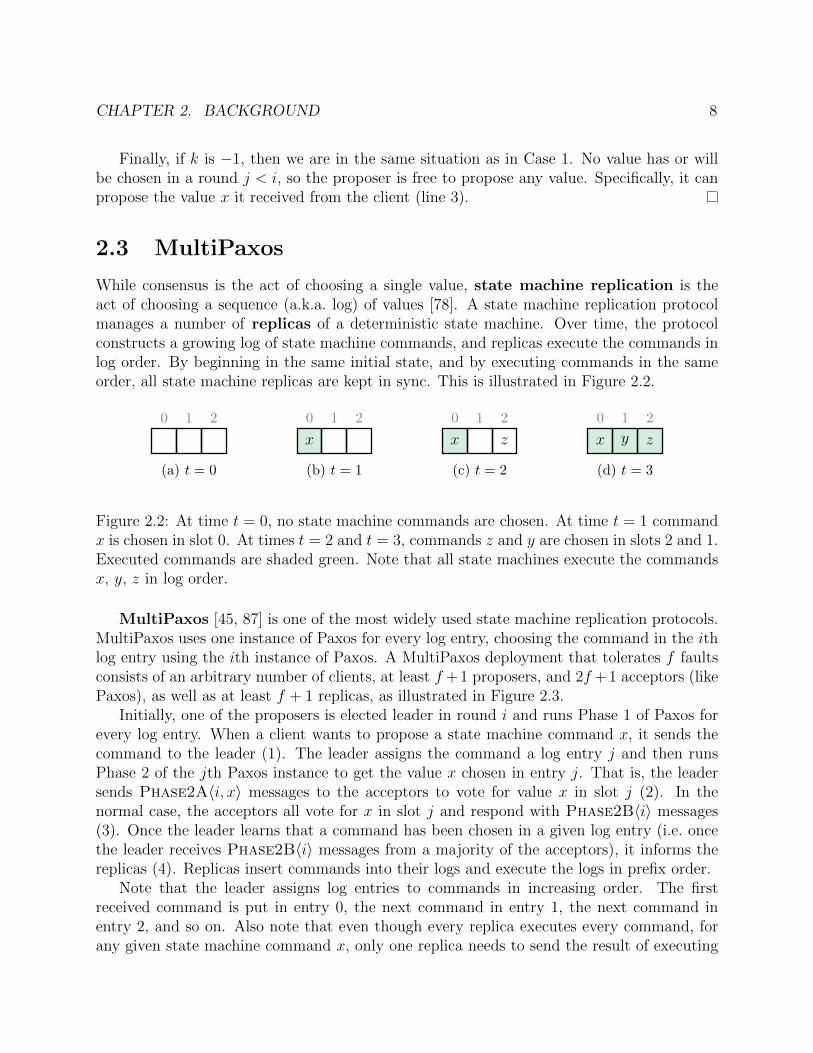
While consensus is the act of choosing a single value, state machine replication is theact of choosing a sequence (a.k.a. log) of values [78]. A state machine replication protocolmanages a number of replicas of a deterministic state machine. Over time, the protocolconstructs a growing log of state machine commands, and replicas execute the commands inlog order. By beginning in the same initial state, and by executing commands in the sameorder, all state machine replicas are kept in sync. This is illustrated in Figure 2.2.
0 1 2
(a) t = 0
x
0 1 2
(b) t = 1
x
0 1
z
2
(c) t = 2
x
0
y
1
z
2
(d) t = 3
Figure 2.2: At time t = 0, no state machine commands are chosen. At time t = 1 commandx is chosen in slot 0. At times t = 2 and t = 3, commands z and y are chosen in slots 2 and 1.Executed commands are shaded green. Note that all state machines execute the commandsx, y, z in log order.
MultiPaxos [45, 87] is one of the most widely used state machine replication protocols.MultiPaxos uses one instance of Paxos for every log entry, choosing the command in the ithlog entry using the ith instance of Paxos. A MultiPaxos deployment that tolerates f faultsconsists of an arbitrary number of clients, at least f +1 proposers, and 2f +1 acceptors (likePaxos), as well as at least f + 1 replicas, as illustrated in Figure 2.3.
Initially, one of the proposers is elected leader in round i and runs Phase 1 of Paxos forevery log entry. When a client wants to propose a state machine command x, it sends thecommand to the leader (1). The leader assigns the command a log entry j and then runsPhase 2 of the jth Paxos instance to get the value x chosen in entry j. That is, the leadersends Phase2A〈i, x〉 messages to the acceptors to vote for value x in slot j (2). In thenormal case, the acceptors all vote for x in slot j and respond with Phase2B〈i〉 messages(3). Once the leader learns that a command has been chosen in a given log entry (i.e. oncethe leader receives Phase2B〈i〉 messages from a majority of the acceptors), it informs thereplicas (4). Replicas insert commands into their logs and execute the logs in prefix order.
Note that the leader assigns log entries to commands in increasing order. The firstreceived command is put in entry 0, the next command in entry 1, the next command inentry 2, and so on. Also note that even though every replica executes every command, forany given state machine command x, only one replica needs to send the result of executing

CHAPTER 2. BACKGROUND 9
c1
c2
c3
p1
p2
a1
a2
a3
r1
r2
Clientsf + 1
Proposers2f + 1
Acceptorsf + 1
Replicas
1 2
23
34
4
5
1 x proposed
2 Phase2A〈i, x〉3 Phase2B〈i〉4 x chosen
5 the result of executing x
Figure 2.3: An example execution of MultiPaxos (f = 1). The leader is adorned with acrown.
x back to the client (5). For example, log entries can be round-robin partitioned across thereplicas.
2.4 Flexible Paxos
Paxos deploys a set of 2f + 1 acceptors, and proposers communicate with at least a majorityof the acceptors in Phase 1 and in Phase 2. While this is sufficient to ensure safety, it is notnecessary. Flexible Paxos [31] is a Paxos variant that generalizes the notion of a majorityto that of a quorum. Specifically, Flexible Paxos uses the notion of a read-write quorumsystem [64]. Given a set A = {a1, . . . , an} of acceptors, a read-write quorum system overA is a pair Q = (R,W ) where
1. R is a set of subsets of A called read quorums (or Phase 1 quorums),
2. W is a set of subsets of W called write quorums (or Phase 2 quorums), and
3. every read quorum intersects every write quorum. That is, for every r ∈ R and w ∈ W ,r ∩ w 6= ∅
Flexible Paxos is identical to Paxos with the exception that proposers now communicatewith an arbitrary Phase 1 quorum in Phase 1 and an arbitrary Phase 2 quorum in Phase 2.This suffices for safety. Flexible MultiPaxos is identical to MultiPaxos, except that it usesFlexible Paxos instead of Paxos. Note that in order for a configuration to tolerate f failures,there must exist some Phase 1 quorum and some Phase 2 quorum of non-failed machinesdespite an arbitrary set of f failures.
10
Chapter 3
Compartmentalization
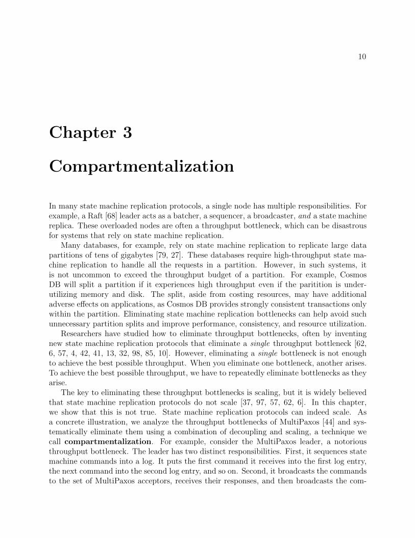
In many state machine replication protocols, a single node has multiple responsibilities. Forexample, a Raft [68] leader acts as a batcher, a sequencer, a broadcaster, and a state machinereplica. These overloaded nodes are often a throughput bottleneck, which can be disastrousfor systems that rely on state machine replication.
Many databases, for example, rely on state machine replication to replicate large datapartitions of tens of gigabytes [79, 27]. These databases require high-throughput state ma-chine replication to handle all the requests in a partition. However, in such systems, itis not uncommon to exceed the throughput budget of a partition. For example, CosmosDB will split a partition if it experiences high throughput even if the paritition is under-utilizing memory and disk. The split, aside from costing resources, may have additionaladverse effects on applications, as Cosmos DB provides strongly consistent transactions onlywithin the partition. Eliminating state machine replication bottlenecks can help avoid suchunnecessary partition splits and improve performance, consistency, and resource utilization.
Researchers have studied how to eliminate throughput bottlenecks, often by inventingnew state machine replication protocols that eliminate a single throughput bottleneck [62,6, 57, 4, 42, 41, 13, 32, 98, 85, 10]. However, eliminating a single bottleneck is not enoughto achieve the best possible throughput. When you eliminate one bottleneck, another arises.To achieve the best possible throughput, we have to repeatedly eliminate bottlenecks as theyarise.
The key to eliminating these throughput bottlenecks is scaling, but it is widely believedthat state machine replication protocols do not scale [37, 97, 57, 62, 6]. In this chapter,we show that this is not true. State machine replication protocols can indeed scale. Asa concrete illustration, we analyze the throughput bottlenecks of MultiPaxos [44] and sys-tematically eliminate them using a combination of decoupling and scaling, a technique wecall compartmentalization. For example, consider the MultiPaxos leader, a notoriousthroughput bottleneck. The leader has two distinct responsibilities. First, it sequences statemachine commands into a log. It puts the first command it receives into the first log entry,the next command into the second log entry, and so on. Second, it broadcasts the commandsto the set of MultiPaxos acceptors, receives their responses, and then broadcasts the com-

CHAPTER 3. COMPARTMENTALIZATION 11
mands again to a set of state machine replicas. To compartmentalize the MultiPaxos leader,we first decouple these two responsibilities. There is no fundamental reason that the leaderhas to sequence commands and broadcast them. Instead, we have the leader sequence com-mands and introduce a new set of nodes, called proxy leaders, to broadcast the commands.Second, we scale up the number of proxy leaders. We note that broadcasting commandsis embarrassingly parallel, so we can increase the number of proxy leaders to avoid thembecoming a bottleneck. Note that this scaling was not possible when sequencing and broad-casting were coupled on the leader since sequencing is not scalable. Compartmentalizationhas three key strengths.
(1) Fast Without Strong Assumptions. We compartmentalize MultiPaxos and in-crease its throughput by over an order of magnitude. Moreover, we achieve our strongperformance without the strong assumptions made by other state machine replication pro-tocols with comparable performance [85, 98, 88, 84, 35]. For example, we do not assume aperfect failure detector [88], we do not assume the availability of specialized hardware [98,84, 35], we do not assume uniform data access patterns [85, 98], we do not assume clocksynchrony [98], and we do not assume key-partitioned state machines [85, 98].
(2) General and Incrementally Adoptable. Compartmentalization is not a pro-tocol. Rather, it is a technique that can be systematically applied to existing protocols.Industry practitioners can incrementally apply compartmentalization to their current proto-cols without having to throw out their battle-tested implementations for something new anduntested. We demonstrate the generality of compartmentalization by applying it to threeother protocols [57, 10, 20] in addition to MultiPaxos.
(3) Easy to Understand. Researchers have invented new state machine replicationprotocols to eliminate throughput bottlenecks, but these new protocols are often subtleand complicated. As a result, these sophisticated protocols have been largely ignored inindustry due to their high barriers to adoption. Compartmentalization is based on the simpleprinciples of decoupling and scaling and is designed to be easily understood. Moreover, inChapter 5, we see how compartmentalization can be used to simplify existing protocols.
In this chapter, we introduce the technique of compartmentalization and use it to com-partmentalize MultiPaxos, Mencius [57], and S-Paxos [10]. Later in Chapter 5, we compart-mentalize more sophisticated state machine replication protocols like EPaxos [62].
3.1 MultiPaxos Does Not Scale?
It is widely believed that MultiPaxos does not scale [37, 97, 57, 62, 6]. Throughout thischapter, we will explain that this is not true, but it first helps to understand why trying toscale MultiPaxos in the straightforward and obvious way does not work. MultiPaxos consistsof proposers, acceptors, and replicas. We discuss each.
First, increasing the number of proposers does not improve performance because everyclient must send its requests to the leader regardless of the number proposers. The non-leaderproposers are idle and do not contribute to the protocol during normal operation.

CHAPTER 3. COMPARTMENTALIZATION 12
Second, increasing the number of acceptors hurts performance. To get a value chosen, theleader must contact a majority of the acceptors. When we increase the number of acceptors,we increase the number of acceptors that the leader has to contact. This decreases through-put because the leader—which is the throughput bottleneck—has to send and receive moremessages per command. Moreover, every acceptor processes at least half of all commandsregardless of the number of acceptors.
Third, increasing the number of replicas hurts performance. The leader broadcasts chosencommands to all of the replicas, so when we increase the number of replicas, we increasethe load on the leader and decrease MultiPaxos’ throughput. Moreover, every replica mustexecute every state machine command, so increasing the number of replicas does not decreasethe replicas’ load.
3.2 Compartmentalizing MultiPaxos
We now compartmentalize MultiPaxos. Throughout this chapter, we introduce six compart-mentalizations, summarized in Table 3.1. For every compartmentalization, we identify athroughput bottleneck and then explain how to decouple and scale it.
Table 3.1: A summary of the compartmentalizations presented in this chapter.
Bottleneck Decouple Scale
1 leader command sequencing and command broadcasting the number of proxy leaders2 acceptors read quorums and write quorums the number of write quorums3 replicas command sequencing and command broadcasting the number of replicas4 leader and replicas read path and write path the number of read quorums5 leader batch formation and batch sequencing the number of batchers6 replicas batch processing and batch replying the number of unbatchers
Compartmentalization 1: Proxy Leaders
Bottleneck: leaderDecouple: command sequencing and broadcastingScale: the number of command broadcasters
Bottleneck The MultiPaxos leader is a well known throughput bottleneck for the followingreason. Refer again to Figure 2.3. To process a single state machine command from a client,the leader must receive a message from the client, send at least f + 1 Phase2A messagesto the acceptors, receive at least f + 1 Phase2B messages from the acceptors, and send atleast f + 1 messages to the replicas. In total, the leader sends and receives at least 3f + 4messages per command. Every acceptor on the other hand processes only 2 messages, and

CHAPTER 3. COMPARTMENTALIZATION 13
every replica processes either 1 or 2. Because every state machine command goes throughthe leader, and because the leader has to perform disproportionately more work than everyother component, the leader is the throughput bottleneck.
Decouple To alleviate this bottleneck, we first decouple the leader. To do so, we note thata MultiPaxos leader has two jobs. The first is sequencing. The leader sequences commandsby assigning each command a log entry. Log entry 0, then 1, then 2, and so on. The secondis broadcasting. The leader sends Phase2A messages, collects Phase2B responses, andbroadcasts chosen values to the replicas. Historically, these two responsibilities have bothfallen on the leader, but this is not fundamental. We instead decouple the two responsibilities.We introduce a set of at least f + 1 proxy leaders, as shown in Figure 3.1. The leaderis responsible for sequencing commands, while the proxy leaders are responsible for gettingcommands chosen and broadcasting the commands to the replicas.
c1
c2
c3
p1
p2
l1
l2
l3
a1
a2
a3
r1
r2
Clientsf + 1
Proposers≥ f + 1
Proxy Leaders2f + 1
Acceptorsf + 1
Replicas
1
23
3
4
4
5
5
6
1 x proposed 2 Phase2A〈i, x〉3 Phase2A〈i, x〉 4 Phase2B〈i〉
5 x chosen 6 the result of executing x
Figure 3.1: An example execution of Compartmentalized MultiPaxos with three proxy lead-ers (f = 1). Throughout the chapter, nodes and messages that were not present in previousiterations of the protocol are highlighted in green.
More concretely, when a leader receives a command x from a client (1), it assigns thecommand x a log entry i and then forms a Phase2A message that includes x and i. Theleader does not send the Phase2A message to the acceptors. Instead, it sends the Phase2Amessage to a randomly selected proxy leader (2). Note that every command can be sent to adifferent proxy leader. The leader balances load evenly across all of the proxy leaders. Uponreceiving a Phase2A message, a proxy leader broadcasts it to the acceptors (3), gathers aquorum of f + 1 Phase2B responses (4), and notifies the replicas of the chosen value (5).All other aspects of the protocol remain unchanged.

CHAPTER 3. COMPARTMENTALIZATION 14
Without proxy leaders, the leader processes 3f + 4 messages per command. With proxyleaders, the leader only processes 2. This makes the leader significantly less of a throughputbottleneck, or potentially eliminates it as the bottleneck entirely.
Scale The leader now processes fewer messages per command, but every proxy leader has toprocess 3f+4 messages. Have we really eliminated the leader as a bottleneck, or have we justmoved the bottleneck into the proxy leaders? To answer this, we note that the proxy leadersare embarrassingly parallel. They operate independently from one another. Moreover, theleader distributes load among the proxy leaders equally, so the load on any single proxyleader decreases as we increase the number of proxy leaders. Thus, we can trivially increasethe number of proxy leaders until they are no longer a throughput bottleneck.
Discussion Note that decoupling enables scaling. As discussed in Section 3.1, we cannotnaively increase the number of proposers. Without decoupling, the leader is both a sequencerand broadcaster, so we cannot increase the number of leaders to increase the number ofbroadcasters because doing so would lead to multiple sequencers, which is not permitted.Only by decoupling the two responsibilities can we scale one without scaling the other.
Also note that the protocol remains tolerant to f faults regardless of the number ofmachines. However, increasing the number of machines does decrease the expected time tof failures (this is true for every protocol that scales up the number of machines, not justour protocol). We believe that increasing throughput at the expense of a shorter time to ffailures is well worth it in practice because failed machines can be replaced with new machinesusing a reconfiguration protocol [44, 68]. The time required to perform a reconfiguration ismany orders of magnitude smaller than the mean time between failures.
Compartmentalization 2: Acceptor Grids
Bottleneck: acceptorsDecouple: read quorums and write quorumsScale: the number of write quorums
Bottleneck After compartmentalizing the leader, it is possible that the acceptors are thethroughput bottleneck. It is widely believed that acceptors do not scale: “using more than2f + 1 [acceptors] for f failures is possible but illogical because it requires a larger quorumsize with no additional benefit” [97]. As explained in Section 3.1, there are two reasons whynaively increasing the number of acceptors is ill-advised.
First, increasing the number of acceptors increases the number of messages that the leaderhas to send and receive. This increases the load on the leader, and since the leader is thethroughput bottleneck, this decreases throughput. This argument no longer applies. Withthe introduction of proxy leaders, the leader no longer communicates with the acceptors.

CHAPTER 3. COMPARTMENTALIZATION 15
Increasing the number of acceptors increases the load on every individual proxy leader, butthe increased load will not make the proxy leaders a bottleneck because we can always scalethem up.
Second, every command must be processed by a majority of the acceptors. Thus, evenwith a large number of acceptors, every acceptor must process at least half of all statemachine commands. This argument still holds.
Decouple We compartmentalize the acceptors by using non-majority read-write quorumsystems [31]. MultiPaxos—the vanilla version, not the compartmentalized version—requires2f + 1 acceptors, and the leader communicates with f + 1 acceptors in both Phase 1 andPhase 2 (a majority of the acceptors). As discussed in Section 2.4, this majority quorumsystem is safe but not necessary. By using other read-write quorum systems, read quorumsdo not have to intersect other read quorums, and write quorums do not have to intersectother write quorums.
By decoupling read quorums from write quorums, we can reduce the load on the acceptorsby using a more efficient quorum system. Specifically, we arrange the acceptors into an r×wrectangular grid, where r, w ≥ f + 1. This is called a grid quorum system. Every rowforms a read quorum, and every column forms a write quorum (r stands for row and forread). That is, a leader contacts an arbitrary row of acceptors in Phase 1 and an arbitrarycolumn of acceptors for every command in Phase 2. Every row intersects every column, sothis is a valid set of quorums.
A 2 × 3 acceptor grid is illustrated in Figure 3.2. There are two read quorums (therows {a1, a2, a3} and {a4, a5, a6}) and three write quorums (the columns {a1, a4}, {a2, a5},{a3, a6}). Because there are three write quorums, every acceptor only processes one thirdof all the commands. This is not possible with majority quorums because with majorityquorums, every acceptor processes at least half of all the commands, regardless of the numberof acceptors.
Scale With majority quorums, every acceptor has to process at least half of all statemachines commands. With grid quorums, every acceptor only has to process 1
wof the state
machine commands. Thus, we can increase w (i.e. increase the number of columns in thegrid) to reduce the load on the acceptors and eliminate them as a throughput bottleneck.
Discussion Note that, like with proxy leaders, decoupling enables scaling. With majorityquorums, read and write quorums are coupled, so we cannot increase the number of acceptorswithout also increasing the size of all quorums. Acceptor grids allow us to decouple thenumber of acceptors from the size of write quorums, allowing us to scale up the acceptorsand decrease their load.
Also note that increasing the number of write quorums increases the size of read quorumswhich increases the number of acceptors that a leader has to contact in Phase 1. We believe

CHAPTER 3. COMPARTMENTALIZATION 16
c1
c2
c3
p1
p2
l1
l2
l3
a1 a2 a3
a4 a5 a6
r1
r2
Clientsf + 1
Proposers≥ f + 1
Proxy Leaders(≥f+1)× (≥f+1)
Acceptorsf + 1
Replicas
1
2 3
3
4
4
5
5
6
1 x proposed 2 Phase2A〈i, x〉3 Phase2A〈i, x〉 4 Phase2B〈i〉
5 x chosen 6 the result of executing x
Figure 3.2: An execution of Compartmentalized MultiPaxos with a 2 × 3 grid of acceptors(f = 1). The two read quorums—{a1, a2, a3} and {a4, a5, a6}—are shown in solid red rect-angles. The three write quorums—{a1, a4}, {a2, a5}, and {a3, a6}—are shown in dashed bluerectangles.
this is a worthy trade-off since Phase 2 is executed in the normal case and Phase 1 is onlyrun in the event of a leader failure.
In this chapter, we use the grid quorum system because it is simple to explain, but it isnot always the most efficient quorum system. In Chapter 4, we take a deep dive into read-quorum systems. We can also use any of these sophisticated read-write quorum systems.
Compartmentalization 3: More Replicas
Bottleneck: replicasDecouple: command sequencing and broadcastingScale: the number of replicas
Bottleneck After compartmentalizing the leader and the acceptors, it is possible that thereplicas are the bottleneck. Recall from Section 3.1 that naively scaling the replicas doesnot work for two reasons. First, every replica must receive and execute every state machinecommand. This is not actually true, but we leave that for the next compartmentalization.Second, like with the acceptors, increasing the number of replicas increases the load on theleader. Because we have already decoupled sequencing from broadcasting on the leader and

CHAPTER 3. COMPARTMENTALIZATION 17
introduced proxy leaders, this is no longer true, so we are free to increase the number ofreplicas. In Figure 3.3, for example, we show MultiPaxos with three replicas instead of theminimum required two.
Scale If every replica has to execute every command, does increasing the number of replicasdecrease their load? Yes. Recall that while every replica has to execute every state machine,only one of the replicas has to send the result of executing the command back to the client.Thus, with n replicas, every replica only has to send back results for 1
nof the commands.
If we scale up the number of replicas, we reduce the number of messages that each replicahas to send. This reduces the load on the replicas and helps prevent them from becominga throughput bottleneck. In Figure 3.3 for example, with three replicas, every replica onlyhas to reply to one third of all commands. With two replicas, every replica has to reply tohalf of all commands. In the next compartmentalization, we’ll see another major advantageof increasing the number of replicas.
c1
c2
c3
p1
p2
l1
l2
l3
a1 a2 a3
a4 a5 a6
r1
r2
r3
Clientsf + 1
Proposers≥ f + 1
Proxy Leaders(≥f+1)× (≥f+1)
Acceptors≥ f + 1Replicas
1
2 3
3
4
4
555
6
1 x proposed 2 Phase2A〈i, x〉3 Phase2A〈i, x〉 4 Phase2B〈i〉
5 x chosen 6 the result of executing x
Figure 3.3: An example execution of Compartmentalized MultiPaxos with three replicas asopposed to the minimum required two (f = 1).
Discussion Again decoupling enables scaling. Without decoupling the leader and intro-ducing proxy leaders, increasing the number of replicas hurts rather than helps performance.

CHAPTER 3. COMPARTMENTALIZATION 18
Compartmentalization 4: Leaderless Reads
Bottleneck: leader and replicasDecouple: read path and write pathScale: the number of read quorums
Bottleneck We have now compartmentalized the leader, the acceptors, and the replicas.At this point, the bottleneck is in one of two places. Either the leader is still a bottleneck,or the replicas are the bottleneck. Fortunately, we can bypass both bottlenecks with a singlecompartmentalization.
Decouple We call commands that modify the state of the state machine writes andcommands that don’t modify the state of the state machine reads. The leader must processevery write because it has to linearize the writes with respect to one another, and everyreplica must process every write because otherwise the replicas’ state would diverge (imagineif one replica performs a write but the other replicas don’t). However, because reads do notmodify the state of the state machine, the leader does not have to linearize them (readscommute), and only a single replica (as opposed to every replica) needs to execute a read.
We take advantage of this observation by decoupling the read path from the write path.Writes are processed as before, but we bypass the leader and perform a read on a singlereplica by using the ideas from Paxos Quorum Reads (PQR) [13]. Specifically, to perform aread, a client sends a PreRead〈〉 message to a read quorum of acceptors. Upon receivinga PreRead〈〉 message, an acceptor ai returns a PreReadAck〈〉 message where wi is theindex of the largest log entry in which the acceptor has voted (i.e. the largest log entry inwhich the acceptor has sent a Phase2B message). We call this wi a vote watermark. Whenthe client receives PreReadAck messages from a read quorum of acceptors, it computes jas the maximum of all received vote watermarks. It then sends a Read〈x, j〉 request to anyone of the replicas where x is an arbitrary read (i.e. a command that does not modify thestate of the state machine).
When a replica receives a Read〈x, j〉 request from a client, it waits until it has executedthe command in log entry j. Recall that replicas execute commands in log order, so ifthe replica has executed the command in log entry j, then it has also executed all of thecommands in log entries less than j. After the replica has executed the command in log entryj, it executes x and returns the result to the client. Note that upon receiving a Read〈x, j〉message, a replica may have already executed the log beyond j. That is, it may have alreadyexecuted the commands in log entries j + 1, j + 2, and so on. This is okay because as longas the replica has executed the command in log entry j, it is safe to execute x.
Scale The decoupled read and write paths are shown in Figure 3.4. Reads are sent to arow (read quorum) of acceptors, so we can increase the number of rows to decrease the readload on every individual acceptor, eliminating the acceptors as a read bottleneck. Reads are

CHAPTER 3. COMPARTMENTALIZATION 19
c1
c2
c3
p1
p2
l1
l2
l3
a1 a2
a3 a4
r1
r2
r3
Clientsf + 1
Proposers≥ f + 1
Proxy Leaders(≥f+1)× (≥f+1)
Acceptors≥ f + 1Replicas
11
2
23
4
1
2 3
3
4
4
555
6
1 x proposed 2 Phase2A〈i, x〉 3 Phase2A〈i, x〉4 Phase2B〈i〉 5 x chosen 6 the result of executing x
1 PreRead〈〉 2 PreReadAck〈〉3 Read〈x, j〉 4 the result of executing x
Figure 3.4: An example execution of Compartmentalized MultiPaxos’ read and write path(f = 1) with a 2× 2 acceptor grid. The write path is shown using solid blue lines. The readpath is shown using red dashed lines.
also sent to a single replica, so we can increase the number of replicas to eliminate them asa read bottleneck as well.
Discussion Note that read-heavy workloads are not a special case. Many workloads areread-heavy [25, 66, 7, 62]. Chubby [11] observes that fewer than 1% of operations are writes,and Spanner [18] observes that fewer than 0.3% of operations are writes.
Also note that increasing the number of columns in an acceptor grid reduces the writeload on the acceptors, and increasing the number of rows in an acceptor grid reduces the readload on the acceptors. There is no throughput trade-off between the two. The number ofrows and columns can be adjusted independently. Increasing read throughput (by increasingthe number of rows) does not decrease write throughput, and vice versa. However, increasingthe number of rows does increase the size (but not number) of columns, so increasing thenumber of rows might increase the tail latency of writes, and vice versa.
Correctness We now define linearizability and prove that our protocol implements lin-earizable reads.

CHAPTER 3. COMPARTMENTALIZATION 20
Linearizability is a correctness condition for distributed systems [28]. Intuitively, a lin-earizable distributed system is indistinguishable from a system running on a single machinethat services all requests serially. This makes a linearizable system easy to reason about.We first explain the intuition behind linearizability and then formalize the intuition.
Consider a distributed system that implements a single register. Clients can send requeststo the distributed system to read or write the register. After a client sends a read or writerequest, it waits to receive a response before sending another request. As a result, a clientcan have at most one operation pending at any point in time.
c1
c2
w(0)OK
w(1)OK
r() 0
(a) An example execution
c1
c2
w(0)OK
w(1)OK
r() 0
(b) An incorrect linearization
c1
c2
w(0)OK
w(1)OK
r() 0
(c) A linearization
Figure 3.5
As a simple example, consider the execution illustrated in Figure 3.5a where the x-axisrepresents the passage of time (real time, not logical time [46]). This execution involves twoclients, c1 and c2. Client c1 sends a w(0) request to the system, requesting that the value 0be written to the register. Then, client c2 sends a w(1) request, requesting that the value 1be written to the register. The system then sends acknowledgments to c1 and c2 before c1sends a read request and receives the value 0.
For every client request, let’s associate the request with a point in time that falls betweenwhen the client sent the request and when the client received the corresponding response.Next, let us imagine that the system executes every request instantaneously at the point intime associated with the request. This hypothetical execution may or may not be consistentwith the real execution.
For example, in Figure 3.5a, we have associated every request with a point halfway be-tween its invocation and response. Thus, in this hypothetical execution, the system executesc1’s w(0) request, then c2’s w(1) request, and finally c1’s r() request. In other words, itwrites 0 into the register, then 1, and then reads the value 1 (the latest value written). Thishypothetical execution is not consistent with the real execution because c1 reads 1 insteadof 0.
Now consider the hypothetical execution in Figure 3.5c in which we execute w(1), thenw(0), and then r(). This execution is consistent with the real execution. Note that c1reads 0 in both executions. Such a hypothetical execution—one that is consistent with thereal execution—is called a linearization. Note that from the clients’ perspective, the realexecution is indistinguishable from its linearization. Maybe the distributed register really isexecuting our requests at exactly the points in time that we selected? There’s no way forthe clients to prove otherwise.

CHAPTER 3. COMPARTMENTALIZATION 21
If an execution has a linearization, we say the execution is linearizable. Similarly, if asystem only allows linearizable executions, we say the system is linearizable. Note that notevery execution is linearizable. The execution in Figure 3.6, for example, is not linearizable.Try to find a linearization. You’ll see that it’s impossible.
c1
c2
c3
w(0)OK r() 1
w(1)OK r() 1
w(0)OK
Figure 3.6: An execution that is not linearizable
We now formalize our intuition on linearizability [28]. A history is a finite sequence ofoperation invocation and response events. For example, the following history:
Hwwr = c1.w(0); c2.w(1); c1.OK; c2.OK; c1.r(); c1.0
is the history illustrated in Figure 3.5a. We draw invocation events in red, and responseevents in blue. We call an invocation and matching response an operation. In Hwwr, everyinvocation is followed eventually by a corresponding response, but this is not always the case.An invocation in a history is pending if there does not exist a corresponding response. Forexample, in the history Hpending below, c2’s invocation is pending:
Hpending = c1.w(0); c2.w(1); c1.OK; c1.r(); c1.0
Hpending is illustrated in Figure 3.7. complete(H) is the subhistory of H that only includesnon-pending operations. For example,
complete(Hpending) = c1.w(0); c1.OK; c1.r(); c1.0
c1
c2
w(0)OK
· · ·w(1)
r() 0
Figure 3.7: A history, Hpending, with a pending invocation

CHAPTER 3. COMPARTMENTALIZATION 22
A client subhistory, H | ci, of a history H is the subsequence of all events in H associ-ated with client ci. Referring again to Hwwr above, we have:
Hwwr | c1 = c1.w(0); c1.OK; c1.r(); c1.0
Hwwr | c2 = c2.w(1); c2.OK
Hwwr | c1 is illustrated in Figure 3.8.
c1w(0)
OK r() 0
Figure 3.8: Hwwr | c1
Two histories H and H ′ are equivalent if for every client ci, H | ci = H ′ | ci. For example,consider the following history:
Hwrw = c1.w(0); c1.OK; c1.r(); c2.w(1); c1.0; c2.OK
Hwrw is illustrated in Figure 3.9. Hwwr is equivalent to Hwrw because
Hwwr | c1 = c1.w(0); c1.OK; c1.r(); c1.0 = Hwrw | c1Hwwr | c2 = c2.w(1); c2.OK; = Hwrw | c2
c1
c2
w(0)OK r() 0
w(1)OK
Figure 3.9: Hwrw
A history H induces an irreflexive partial order <H on operations where o1 <H o2 if theresponse of o1 precedes the invocation of o2 in H. If o1 <H o2, we say o1 happens beforeo2. In Hwwr for example, c2’s operation happens before c1’s second operation. In Hwrw, onthe other hand, the two operations are not ordered by the happens before relation. Thisshows that equivalent histories may not have the same happens before relation.
Finally, a history H is linearizable if it can be extended (by appending zero or moreresponse events) to some history H ′ such that (a) complete(H ′) is equivalent to some se-quential history S, and (b) <S respects <H (i.e. if two operations are ordered in H, theymust also be ordered in S). S is called a linearization. The history Hwwr, for example, islinearizable with the linearization
Swwr = c2.w(1); c2.OK; c1.w(0); c1.OK; c1.r(); c1.0

CHAPTER 3. COMPARTMENTALIZATION 23
c1
c2w(1)
OK
w(0)OK r() 0
Figure 3.10: Swrw
illustrated in Figure 3.10We now prove that our protocol correctly implements linearizable reads.
Proof. Let H be an arbitrary history permitted by our protocol. To prove that our protocolis linearizable, we must extend H to a history H ′ such that complete(H ′) is equivalent to asequential history that respects <H .
Recall that extending H to H ′ is sometimes necessary because of situations like the oneshown in Figure 3.11. This example involves a single register with an initial value of 0. c1issues a request to write the value of 1, but has not yet received a response. c2 issues a readrequest and receives the value 1. If we do not extend the history to include a response toc1’s write, then there will not exist an equivalent sequential history.
c1
c2
· · ·w(1)
r() 1
Figure 3.11: A motivating example of history extension
So, which operations should we include in H ′? Let k be the largest log index writtenin or read from in complete(H). First note that for every index 0 ≤ i ≤ k, there exists a(potentially pending) write in H that has been chosen in index i. Why? Well, our protocolexecutes commands in log order, so a write at index k can only complete after all writeswith smaller indices have been chosen (and executed by some replica). Similarly, if a readoperation reads from slot k, then the write in slot k must have been executed, so again allwrites with smaller indices have also been chosen. We extend H to history H ′ by includingresponses for all pending write invocations with indices 0 ≤ i ≤ k. The responses are formedby executing the k + 1 commands in log order.
For example, consider the history G shown in Figure 3.12. wi represents a write chosenin log index i, ri represents a read operation that reads from slot i, w? represents a pendingwrite which has not been chosen in any particular log index, and r? represents a pendingread. complete(G) includes w1 and r2, so here k = 2 and we must include all writes in indices

CHAPTER 3. COMPARTMENTALIZATION 24
0, 1, and 2. That is, we extend G to complete w0 and w2. w4 is left pending, as is w? andr?. Also note that we could not complete w4 even if we wanted to because there is no w3.
c1
c2
c3
c4
c5
· · ·w0
w1· · ·w2
r2 · · ·w4
r2 · · ·w?
· · ·r?
Figure 3.12: An example history G. Responses are not shown, as they are not important forthis example.
Now, we must prove that (1) complete(H ′) is equivalent to some legal sequential historyS, and (2) <S respects <H . We let S be the sequential history formed from executing allwrites in log order and from executing every read from index i after the write in index i.If there are multiple reads from index i, the reads are ordered in an arbitrary way thatrespects <H . For example, the history G in Figure 3.12 has the sequential history SG shownin Figure 3.13. Note that c4’s read comes after c3’s read. This is essential because we mustrespect <G. If the two reads were concurrent in G, they could be ordered arbitrarily in SG.
c1
c2
c3
c4
w0
w1 w2
r2
r2
Figure 3.13: A linearization SG of the history in G Figure 3.12
To prove (1) and (2), we show that if two distinct operations x and y that write to(or read from) log indices i and j are related in H—i.e. x <H y, or x finishes before ybegins—then i ≤ j. We perform a case analysis on whether x and y are reads or writes.
• x and y are both writes: At the time x completes in index i, all commands inindices less than i have been chosen because our protocol executes commands in log

CHAPTER 3. COMPARTMENTALIZATION 25
order. Thus, when y later begins, it cannot be chosen in a log entry less than i, sinceevery log entry implements consensus. Thus, i < j.
• x and y are both reads: When x completes, command i has been chosen. Thus,some write quorum w of acceptors must have voted for the command in log entry i.When y begins, it sends PreRead messages to some read quorum r of acceptors. rand w intersect, so the client executing y will receive a PreReadAck〈wi〉 messagefrom some acceptor in r with wi ≥ i. Therefore, y is guaranteed to read from somej ≥ i.
• x is a read and y is a write: When x completes, all commands in indices i andsmaller have been chosen. By the first case above, y must be chosen in some indexj > i.
• x is a write and y is a read: When x completes, command i has been chosen. Aswith the second case above, when y begins it will contact an acceptor group with avote watermark at least as large as i and will subsequently read from at least i.
From this, (1) is immediate since every client’s operations are in the same order in H ′
and in S. (2) holds because S is ordered by log index with ties broken respecting <H , so ifx <H y, then i ≤ j and x <S y.
Non-Linearizable Reads Our protocol implements linearizable reads, the strongest formof non-transactional consistency. However, we can extend the protocol to support readswith better performance but weaker consistency. Notably, we can implement sequentiallyconsistent [43] and eventually consistent reads. Writes are always linearizable. The decisionof which consistency level to choose depends on the application.
Sequential consistency is a lot like linearizability but without the real-time orderingrequirements. Specifically, a history H is sequentially consistent if we can extend it to somehistory H ′ such that complete(H ′) is equivalent to some sequential history S. Unlike withlinearizability, we do not require that <S respects <H .
To implement sequentially consistent reads, every client needs to (a) keep track of thelargest log entry it has ever written to or read from, and (b) make sure that all futureoperations write to or read from a log entry as least as large. Concretely, we make thefollowing changes:
• Every client ci maintains an integer-valued watermark wi, initially −1.
• When a replica executes a write w in log entry j and returns the result of executingw to a client ci, it also includes j. When ci receives a write index j from a replica, itupdates wi to the max of wi and j.
• To execute a sequentially consistent read r, a client ci sends a Read〈r, wi〉 message toany replica. The replica waits until it has executed the write in log entry wi and then

CHAPTER 3. COMPARTMENTALIZATION 26
executes r. It then replies to the client with the result of executing r and the log entryj from which r reads. Here, j ≥ wi. When a client receives a read index j, it updateswi to the max of wi and j.
Note that a client can finish a sequentially consistent read after one round-trip of com-munication (in the best case), whereas a linearizable read requires at least two. Moreover,sequentially consistent reads do not involve the acceptors. This means that we can increaseread throughput by scaling up the number of replicas without having to scale up the numberof acceptors. Also note that sequentially consistent reads are also causally consistent.
Eventually consistent reads are trivial to implement. To execute an eventually consistentread, a client simply sends the read request r directly to any replica. The replica executesthe read immediately and returns the result back to the client. Eventually consistent readsdo not require any watermark bookkeeping, do not involve acceptors, and never wait forwrites. Moreover, the reads are always executed against a consistent prefix of the log.
3.3 Batching
All state machine replication protocols, including MultiPaxos, can take advantage of batchingto increase throughput. The standard way to implement batching [77, 76] is to have clientssend their commands to the leader and to have the leader group the commands together intobatches, as shown in Figure 3.14. The rest of the protocol remains unchanged, with commandbatches replacing commands. The one notable difference is that replicas now execute onebatch of commands at a time, rather than one command at a time. After executing a singlecommand, a replica has to send back a single result to a client, but after executing a batchof commands, a replica has to send a result to every client with a command in the batch.
Compartmentalization 5: Batchers
Bottleneck: leaderDecouple: batch formation and batch sequencingScale: the number of batchers
Bottleneck We first discuss write batching and discuss read batching momentarily. Batch-ing increases throughput by amortizing the communication and computation cost of process-ing a command. Take the acceptors for example. Without batching, an acceptor processestwo messages per command. With batching, however, an acceptor only processes two mes-sages per batch. The acceptors process fewer messages per command as the batch sizeincreases. With batches of size 10, for example, an acceptor processes 10× fewer messagesper command with batching than without.
Refer again to Figure 3.14. The load on the proxy leaders and the acceptors both decreaseas the batch size increases, but this is not the case for the leader or the replicas. We focus first

CHAPTER 3. COMPARTMENTALIZATION 27
c1
c2
c3
p1
p2
l1
l2
l3
a1 a2
a3 a4
r1
r2
r3
Clientsf + 1
Proposers≥ f + 1
Proxy Leaders(≥f+1)× (≥f+1)
Acceptors≥ f + 1Replicas
1
1
1
2 3
3
4
4
555
6
6
6
1 x, y, z proposed 2 Phase2A〈i, {x, y, z}〉3 Phase2A〈i, {x, y, z}〉 4 Phase2B〈i〉
5 {x, y, z} chosen 6 the results of executing x, y, and z
Figure 3.14: An example execution of Compartmentalized MultiPaxos with batching (f = 1).Messages that contain a batch of commands, rather than a single command, are drawnthicker. Note how replica r2 has to send multiple messages after executing a batch of com-mands.
on the leader. To process a single batch of n commands, the leader has to receive n messagesand send one message. Unlike the proxy leaders and acceptors, the leader’s communicationcost is linear in the number of commands rather than the number of batches. This makesthe leader a very likely throughput bottleneck.
Decouple The leader has two responsibilities. It forms batches, and it sequences batches.We decouple the two responsibilities by introducing a set of at least f + 1 batchers, asillustrated in Figure 3.15. The batchers are responsible for forming batches, while the leaderis responsible for sequencing batches.
More concretely, when a client wants to propose a state machine command, it sends thecommand to a randomly selected batcher (1). After receiving sufficiently many commandsfrom the clients (or after a timeout expires), a batcher places the commands in a batch andforwards it to the leader (2). When the leader receives a batch of commands, it assigns it alog entry, forms a Phase 2a message, and sends the Phase2a message to a proxy leader(3). The rest of the protocol remains unchanged.
Without batchers, the leader has to receive n messages per batch of n commands. Withbatchers, the leader only has to receive one. This either reduces the load on the bottleneckleader or eliminates it as a bottleneck completely.

CHAPTER 3. COMPARTMENTALIZATION 28
c1
c2
c3
b1
b2
b3
p1
p2
l1
l2
l3
a1 a2
a3 a4
r1
r2
r3
Clients≥ f + 1Batchers
f + 1Proposers
≥ f + 1ProxyLeaders
(≥f+1)× (≥f+1)Acceptors
≥ f + 1Replicas
1
1
1
2
3 4
4
5
5
666
7
7
7
1 x, y, z proposed 2 {x, y, z}3 Phase2A〈i, {x, y, z}〉 4 Phase2A〈i, {x, y, z}〉
5 Phase2B〈i〉 6 {x, y, z} chosen
7 the results of executing x, y, and z
Figure 3.15: An example execution of Compartmentalized MultiPaxos with batchers (f = 1).
Scale The batchers are embarrassingly parallel. We can increase the number of batchersuntil they’re not a throughput bottleneck.
Discussion Read batching is very similar to write batching. Clients send reads to ran-domly selected batchers, and batchers group reads together into batches. After a batcherhas formed a read batch X, it sends a PreRead〈〉 message to a read quorum of accep-tors, computes the resulting watermark i, and sends a Read〈X, i〉 request to any one of thereplicas.
Compartmentalization 6: Unbatchers
Bottleneck: replicasDecouple: batch processing and batch replyingScale: the number of unbatchers
Bottleneck After executing a batch of n commands, a replica has to send n messages backto the n clients. Thus, the replicas (like the leader without batchers) suffer communicationoverheads linear in the number of commands rather than the number of batches.
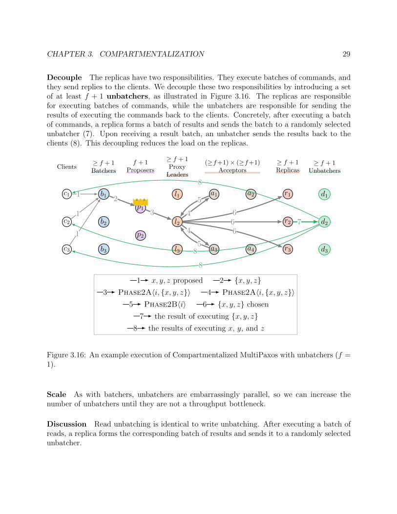
CHAPTER 3. COMPARTMENTALIZATION 29
Decouple The replicas have two responsibilities. They execute batches of commands, andthey send replies to the clients. We decouple these two responsibilities by introducing a setof at least f + 1 unbatchers, as illustrated in Figure 3.16. The replicas are responsiblefor executing batches of commands, while the unbatchers are responsible for sending theresults of executing the commands back to the clients. Concretely, after executing a batchof commands, a replica forms a batch of results and sends the batch to a randomly selectedunbatcher (7). Upon receiving a result batch, an unbatcher sends the results back to theclients (8). This decoupling reduces the load on the replicas.
c1
c2
c3
b1
b2
b3
p1
p2
l1
l2
l3
a1 a2
a3 a4
r1
r2
r3
d1
d2
d3
Clients≥ f + 1Batchers
f + 1Proposers
≥ f + 1ProxyLeaders
(≥f+1)× (≥f+1)Acceptors
≥ f + 1Replicas
≥ f + 1Unbatchers
1
1
1
2
3 4
4
5
5
666
7
8
8
8
1 x, y, z proposed 2 {x, y, z}3 Phase2A〈i, {x, y, z}〉 4 Phase2A〈i, {x, y, z}〉
5 Phase2B〈i〉 6 {x, y, z} chosen
7 the result of executing {x, y, z}8 the results of executing x, y, and z
Figure 3.16: An example execution of Compartmentalized MultiPaxos with unbatchers (f =1).
Scale As with batchers, unbatchers are embarrassingly parallel, so we can increase thenumber of unbatchers until they are not a throughput bottleneck.
Discussion Read unbatching is identical to write unbatching. After executing a batch ofreads, a replica forms the corresponding batch of results and sends it to a randomly selectedunbatcher.

CHAPTER 3. COMPARTMENTALIZATION 30
3.4 Mencius
Background
As discussed previously, the MultiPaxos leader is a throughput bottleneck because all com-mands go through the leader and because the leader performs disproportionately more workper command than the acceptors or replicas. Mencius is a MultiPaxos variant that attemptsto eliminate this bottleneck by using more than one leader.
Rather than having a single leader sequence all commands in the log, Mencius round-robin partitions the log among multiple leaders. For example, consider the scenario withthree leaders l1, l2, and l3 illustrated in Figure 3.17. Leader l1 gets commands chosen inslots 0, 3, 6, etc.; leader l2 gets commands chosen in slots 1, 4, 7, etc.; and leader l3 getscommands chosen in slots 2, 5, 8, etc.
0
l1
1
l2
2
l3
3
l1
4
l2
5
l3
6
l1
. . .
l1
l2
l3
0, 3, 6, . . .
1, 4, 7, . . .
2, 5, 8, . . .
Figure 3.17: A Mencius log round robin partitioned among three leaders.
Having multiple leaders works well when all the leaders process commands at the exactsame rate. However, if one of the leaders is slower than the others, then holes start appearingin the log entries owned by the slow leader. This is illustrated in Figure 3.18a. Figure 3.18adepicts a Mencius log partitioned across three leaders. Leaders l1 and l2 have both gottena few commands chosen (e.g., a in slot 0, b in slot 1, etc.), but leader l3 is lagging behindand has not gotten any commands chosen yet. Replicas execute commands in log order, sothey are unable to execute all of the chosen commands until l3 gets commands chosen in itsvacant log entries.
If a leader detects that it is lagging behind, then it fills its vacant log entries with asequence of noops. A noop is a distinguished command that does not affect the state ofthe replicated state machine. In Figure 3.18b, we see that l3 fills its vacant log entries withnoops. This allows the replicas to execute all of the chosen commands.
More concretely, a Mencius deployment that tolerates f faults is implemented with 2f+1servers, as illustrated in Figure 3.19. Roughly speaking, every Mencius server plays the roleof a MultiPaxos leader, acceptor, and replica.
When a client wants to propose a state machine command x, it sends x to any of theservers (1). Upon receiving command x, a server sl plays the role of a leader. It assigns thecommand x a slot i and sends a Phase 2a message that includes x and i to the other servers

CHAPTER 3. COMPARTMENTALIZATION 31
a
0
l1
b
1
l2
2
l3
c
3
l1
d
4
l2
5
l3
e
6
l1
f
7
l2
8
l3
g
9
l1
. . .
(a) Before noops
a
0
l1
b
1
l2
noop
2
l3
c
3
l1
d
4
l2
noop
5
l3
e
6
l1
f
7
l2
noop
8
l3
g
9
l1
. . .
(b) After noops
Figure 3.18: An example of using noops to deal with a slow leader. Leader l3 is slowerthan leaders l1 and l2, so the log has holes in l3’s slots. l3 fills its holes with noops to allowcommands in the log to be executed.
c1
c2
c3
s1
s2
s3
Clients 2f + 1 Servers
1
234
234
4
Figure 3.19: An example execution of Mencius.
(2). Upon receiving a Phase 2a message, a server sa plays the role of an acceptor and replieswith a Phase 2b message (3).
In addition, sa uses i to determine if it is lagging behind sl. If it is, then it sends a skipmessage along with the Phase 2b message. The skip message informs the other servers tochoose a noop in every slot owned by sa up to slot i. For example, if a server sa’s nextavailable slot is slot 10 and it receives a Phase 2a message for slot 100, then it broadcastsa skip message informing the other servers to place noops in all of the slots between slots10 and 100 that are owned by server sa. Mencius leverages a protocol called CoordinatedPaxos to ensure noops are chosen correctly. We refer to the reader to [57] for details.
Upon receiving Phase 2b messages for command x from a majority of the servers, serversl deems the command x chosen. It informs the other servers that the command has been

CHAPTER 3. COMPARTMENTALIZATION 32
chosen and also sends the result of executing x back to the client.
Compartmentalization
Mencius uses multiple leaders to avoid being bottlenecked by a single leader. However,despite this, Mencius still does not achieve optimal throughput. Part of the problem isthat every Mencius server plays three roles, that of a leader, an acceptor, and a replica.Because of this, a server has to send and receive a total of roughly 3f + 5 messages for everycommand that it leads and also has to send and receive messages acking other servers asthey simultaneously choose commands.
We can solve this problem by decoupling the servers. Instead of deploying a set of heavilyloaded servers, we instead view Mencius as a MultiPaxos variant and deploy it as a set ofproposers, a set of acceptors, and set of replicas. This is illustrated in Figure 3.20.
c1
c2
c3
p1
p2
p3
a1
a2
a3
r1
r2
Clients≥ f + 1Leaders
2f + 1Acceptors
f + 1Replicas
12
2
3
3
4
4
5
Figure 3.20: An example execution of decoupled Mencius. Note that every proposer is aleader.
Now, Mencius is equivalent to MultiPaxos with the following key differences. First, everyproposer is a leader, with the log round-robin partitioned among all the proposers. If aclient wants to propose a command, it can send it to any of the proposers. Second, theproposers periodically broadcast their next available slots to one another. Every server usesthis information to gauge whether it is lagging behind. If it is, it chooses noops in its vacantslots, as described above.
This decoupled Mencius is a step in the right direction, but it shares many of the problemsthat MultiPaxos faced. The proposers are responsible for both sequencing commands andfor coordinating with acceptors; we have a single unscalable group of acceptors; and weare deploying too few replicas. Thankfully, we can compartmentalize Mencius in exactly thesame way as MultiPaxos by leveraging proxy leaders, acceptor grids, and more replicas. Thisis illustrated in Figure 3.21.

CHAPTER 3. COMPARTMENTALIZATION 33
c1
c2
c3
p1
p2
p3
l1
l2
l3
a1 a2
a3 a4
r1
r2
r3
Clients≥ f + 1Leaders
≥ f + 1Proxy Leaders
(≥f+1)× (≥f+1)Acceptors
≥ f + 1Replicas
1
23
3
4
4
5
5
5
6
Figure 3.21: An execution of Mencius with proxy leaders, acceptor grids, and an increasednumber of replicas.
This protocol shares all of the advantages of compartmentalized MultiPaxos. Proxy lead-ers and acceptors both trivially scale so are not bottlenecks, while leaders and replicas havebeen pared down to their essential responsibilities of sequencing and executing commandsrespectively. Moreover, because Mencius allows us to deploy multiple leaders, we can alsoincrease the number of leaders until they are no longer a bottleneck. We can also intro-duce batchers and unbatchers like we did with MultiPaxos and can implement linearizableleaderless reads.
3.5 S-Paxos
Background
S-Paxos [10] is a MultiPaxos variant that, like Mencius, aims to avoid being bottlenecked bya single leader. Recall that when a MultiPaxos leader receives a state machine command xfrom a client, it broadcasts a Phase 2a message to the acceptors that includes the command x.If the leader receives a state machine command that is large (in terms of bytes) or receives alarge batch of modestly sized commands, the overheads of disseminating the commands beginto dominate the cost of the protocol, exacerbating the fact that command disseminating isperformed solely by the leader.
S-Paxos avoids this by decoupling command dissemination from command sequencing—separating control from from data flow—and distributing command dissemination across allnodes. More concretely, an S-Paxos deployment that tolerates f faults consists of 2f + 1servers, as illustrated in Figure 3.22. Every server plays the role of a MultiPaxos proposer,acceptor, and replica. It also plays the role of a disseminator and stabilizer, two rolesthat will become clear momentarily.

CHAPTER 3. COMPARTMENTALIZATION 34
c1
c2
c3
s1
s2
s3
Clients 2f + 1 Servers
1
2
2
3
3
3
3
(a) Dissemination
c1
c2
c3
s1
s2
s3
Clients 2f + 1 Servers
456
456
7
(b) Ordering
Figure 3.22: An example execution of S-Paxos. Messages that include client commands (asopposed to ids) are bolded.
When a client wants to propose a state machine command x, it sends x to any of theservers. Upon receiving a command from a client, a server plays the part of a disseminator.It assigns the command a globally unique id idx and begins a dissemination phase withthe goal of persisting the command and its id on at least a majority of the servers. This isshown in Figure 3.22a. The server broadcasts x and idx to the other servers. Upon receivingx and idx, a server plays the role of a stabilizer and stores the pair in memory. It thenbroadcasts an acknowledgement to all servers. The acknowledgement contains idx but notx.
One of the servers is the MultiPaxos leader. Upon receiving acknowledgements for idxfrom a majority of the servers, the leader knows the command is stable. It then uses theid idx as a proxy for the corresponding command x and runs the MultiPaxos protocol asusual (i.e. broadcasting Phase 2a messages, receiving Phase 2b messages, and notifying theother servers when a command id has been chosen) as shown in Figure 3.22b. Thus, whileMultiPaxos agrees on a log of commands, S-Paxos agrees on a log of command ids.
The S-Paxos leader, like the MultiPaxos leader, is responsible for ordering command idsand getting them chosen. But, the responsibility of disseminating commands is shared byall the servers.
Compartmentalization
We compartmentalize S-Paxos similar to how we compartmentalize MultiPaxos and Mencius.First, we decouple servers into a set of at least f+1 disseminators, a set of 2f+1 stabilizers,a set of proposers, a set of acceptors, and a set of replicas. This is illustrated in Figure 3.23.To propose a command x, a client sends it to any of the disseminators. Upon receiving x, adisseminator persists the command and its id idx on at least a majority of (and typically all

CHAPTER 3. COMPARTMENTALIZATION 35
of) the stabilizers. It then forwards the id to the leader. The leader gets the id chosen in aparticular log entry and informs one of the stabilizers. Upon receiving idx from the leader,the stabilizer fetches x from the other stabilizers if it has not previously received it. Thestabilizer then informs the replicas that x has been chosen. Replicas execute commands inprefix order and reply to clients as usual.
c1
c2
c3
d1
d2
s1
s2
s3
p1
p2
a1
a2
a3
r1
r2
Clients≥ f + 1
Disseminators2f + 1
Stabilizers
≥ f + 1Proposers
2f + 1Acceptors
f + 1Replicas
1
2
2
2
3
3
3
45
56
6
7
8
8
9
Figure 3.23: An example execution of decoupled S-Paxos. Messages that include clientcommands (as opposed to ids) are bolded. Note that the MultiPaxos leader does not sendor receive any messages that include a command, only messages that include command ids.
Though S-Paxos relieves the MultiPaxos leader of its duty to broadcast commands, theleader still has to broadcast command ids. In other words, the leader is no longer a bottle-neck on the data path but is still a bottleneck on the control path. Moreover, disseminatorsand stabilizers are potential bottlenecks. We can resolve these issues by compartmentaliz-ing S-Paxos similar to how we compartmentalized MultiPaxos. We introduce proxy leaders,acceptor grids, and more replicas. Moreover, we can trivially scale up the number of dissem-inators; we can deploy stabilizer grids; and we can implement linearizable leaderless reads.This is illustrated in Figure 3.24. To support batching, we can again introduce batchers andunbatchers.
3.6 Evaluation
Latency-Throughput
Experiment Description We call MultiPaxos with the six compartmentalizations de-scribed in this chapter Compartmentalized MultiPaxos. We implemented MultiPaxos,Compartmentalized MultiPaxos, and an unreplicated state machine in Scala using the Netty

CHAPTER 3. COMPARTMENTALIZATION 36
c1
c2
c3
d1
d2
d3
s1 s2
s3 s4
p1
p2
l1
l2
l3
a1 a2
a3 a4
r1
r2
r3
Clients ≥ f + 1Disseminators
(≥f+1)× (≥f+1)Stabilizers (≥f+1)× (≥f+1)
Acceptors≥ f + 1Proposers
≥ f + 1ProxyLeaders
≥ f + 1Replicas
1
2
2
3
3
4 56
6
7
7
8
99
9
10
Figure 3.24: An example execution of S-Paxos with stabilizer grids, proxy leaders, acceptorgrids, and an increased number of replicas. Messages that include client commands (asopposed to ids) are bolded.
networking library (see github.com/mwhittaker/frankenpaxos). MultiPaxos employs 2f + 1machines with each machine playing the role of a MultiPaxos proposer, acceptor, and replica.The unreplicated state machine is implemented as a single process on a single server. Clientssend commands directly to the state machine. Upon receiving a command, the state machineexecutes the command and immediately sends back the result. Note that unlike MultiPaxosand Compartmentalized MultiPaxos, the unreplicated state machine is not fault tolerant. Ifthe single server fails, all state is lost and no commands can be executed. Thus, the unrepli-cated state machine should not be viewed as an apples-to-apples comparison with the othertwo protocols. Instead, the unreplicated state machine sets an upper bound on attainableperformance.
We measure the throughput and median latency of the three protocols under workloadswith a varying numbers of clients. Each client issues state machine commands in a closedloop. It waits to receive the result of executing its most recently proposed command beforeit issues another. All three protocols replicate a key-value store state machine where thekeys are integers and the values are 16 byte strings. In this benchmark, all state machinecommands are writes. There are no reads. Note that multiple clients are run within a singleprocess, so the number of physical client processes can be significantly less than the numberof logical clients.
We deploy the protocols with and without batching for f = 1. Without batching, wedeploy Compartmentalized MultiPaxos with two proposers, ten proxy leaders, a two by twogrid of acceptors, and four replicas. With batching, we deploy two batchers, two proposers,three proxy replicas, a simple majority quorum system of three acceptors, two replicas, andthree unbatchers. For simplicity, every node is deployed on its own machine, but in practice,

CHAPTER 3. COMPARTMENTALIZATION 37
0 50 100 150 200 250Throughput (thousands of commands per second)
0.0
2.5
5.0
7.5
10.0
Med
ian
late
ncy
(ms)
MultiPaxosCompartmentalized MultiPaxosUnreplicated
(a) Without batching
0 200 400 600 800 1000Throughput (thousands of commands per second)
0
5
10
15
Med
ian
late
ncy
(ms)
MultiPaxosCompartmentalized MultiPaxosUnreplicated
(b) With batching
Figure 3.25: The latency and throughput of MultiPaxos, Compartmentalized MultiPaxos,and an unreplicated state machine.
nodes can be physically co-located. In particular, any two logical roles can be placed on thesame machine without violating fault tolerance constraints, so long as the two roles are notthe same.
We deploy the three protocols on AWS using a set of m5.xlarge machines within a singleavailability zone. Every m5.xlarge instance has 4 vCPUs and 16 GiB of memory. Everythingis done in memory, and nothing is written to disk (because everything is replicated, datais persistent even without writing it to disk). In our experiments, the network is never abottleneck. All numbers presented are the average of three executions of the benchmark. Asis standard, we implement MultiPaxos and Compartmentalized MultiPaxos with thriftinessenabled [62]. For a given number of clients, the batch size is set empirically to optimizethroughput. For a fair comparison, we deploy the unreplicated state machine with a set ofbatchers and unbatchers when batching is enabled.
Results The results of the experiment are shown in Figure 3.25. The standard deviationof throughput measurements are shown as a shaded region. Without batching, MultiPaxoshas a peak throughput of roughly 25,000 commands per second, while CompartmentalizedMultiPaxos has a peak throughput of roughly 150,000 commands per second, a 6× increase.The unreplicated state machine outperforms both protocols. It achieves a peak throughputof roughly 250,000 commands per second. Compartmentalized MultiPaxos underperformsthe unreplicated state machine because—despite decoupling the leader as much as possible—the single leader remains a throughput bottleneck. Note that after fully compartmentalizingMultiPaxos, either the leader or the replicas are guaranteed to be the throughput bottle-

CHAPTER 3. COMPARTMENTALIZATION 38
neck because all other components (e.g., proxy leaders, acceptors, batchers, unbatchers) canbe scaled arbitrarily. Implementation and deployment details (e.g., what state machine isbeing replicated) determine which component is the ultimate throughput bottleneck. Allthree protocols have millisecond latencies at peak throughput. With batching, MultiPaxos,Compartmentalized MultiPaxos, and the unreplicated state machine have peak throughputsof roughly 200,000, 800,000 and 1,000,000 commands per second respectively.
Compartmentalized MultiPaxos uses 6.66× more machines than MultiPaxos. On thesurface, this seems like a weakness, but in reality it is a strength. MultiPaxos does not scale,so it is unable to take advantage of more machines. Compartmentalized MultiPaxos, on theother hand, achieves a 6× increase in throughput using 6.66× the number of resources. Thus,we achieve 90% of perfect linear scalability. In fact, with the mixed read-write workloadsbelow, we are able to scale throughput superlinearly with the number of resources. This isbecause compartmentalization eliminates throughput bottlenecks. With throughput bottle-necks, non-bottlenecked components are underutilized. When we eliminate the bottlenecks,we eliminate underutilization and can increase performance without increasing the numberof resources. Moreover, a protocol does not have to be fully compartmentalized. We canselectively compartmentalize some but not all throughput bottlenecks to reduce the numberof resources needed. In other words, MultiPaxos and Compartmentalized MultiPaxos arenot two alternatives, but rather two extremes in a trade-off between throughput and resourceusage.
We also compared the unbatched performance of Compartmentalized MultiPaxos andthe unreplicated state machine with values being 100 bytes and 1000 bytes. The results areshown in Figure 3.26. Expectedly, the protocols’ peak throughput decreases as we increasethe value size.
Ablation Study
Experiment Description We now perform an ablation study to measure the effect of eachcompartmentalization. In particular, we begin with MultiPaxos and then decouple and scalethe protocol according to the six compartmentalizations, measuring peak throughput alongthe way. Note that we cannot measure the effect of each individual compartmentalizationin isolation because decoupling and scaling a component only improves performance if thatcomponent is a bottleneck. Thus, to measure the effect of each compartmentalization, wehave to apply them all, and we have to apply them in an order that is consistent with theorder in which bottlenecks appear. All the details of this experiment are the same as theprevious experiment unless otherwise noted.
Results The unbatched ablation study results are shown in Figure 3.27a. MultiPaxos hasa throughput of roughly 25,000 commands per second. When we decouple the protocol andintroduce proxy leaders (Section 3.2), we increase the throughput to roughly 70,000 com-mands per second. This decoupled MultiPaxos uses the bare minimum number of proposers(2), proxy leaders (2), acceptors (3), and replicas (2). We then scale up the number of proxy

CHAPTER 3. COMPARTMENTALIZATION 39
0 50 100 150 200Throughput (thousands of commands per second)
0
2
4
6
8
10
Med
ian
late
ncy
(ms)
Compartmentalized MultiPaxos (100 bytes)Unreplicated (100 bytes)Compartmentalized MultiPaxos (1000 bytes)Unreplicated (1000 bytes)
Figure 3.26: The latency and throughput of Compartmentalized MultiPaxos and an unrepli-cated state machine without batching and with larger value sizes.
coupled
decoupled
3 proxy leaders
4 proxy leaders
5 proxy leaders
6 proxy leaders
7 proxy leaders
3 replicas
8 proxy leaders
9 proxy leaders
10 proxy leaders
0
50
100
150
Thro
ughp
ut(th
ousa
nds c
mds
/sec
ond)
(a) Without batching
coupled
decoupled
batch size 50
batch size 100
3 unbatchers
4 unbatchers
5 unbatchers
0
200
400
600
Thro
ughp
ut(th
ousa
nds c
mds
/sec
ond)
(b) With batching
Figure 3.27: An ablation study. Standard deviations are shown using error bars.
leaders from 2 to 7. The proxy leaders are the throughput bottleneck, so as we scale themup, the throughput of the protocol increases until it plateaus at roughly 135,000 commandsper second. At this point, the proxy leaders are no longer the throughput bottleneck; thereplicas are. We introduce an additional replica (Section 3.2), though the throughput doesnot increase. This is because proxy leaders broadcast commands to all replicas, so introduc-ing a new replica increases the load on the proxy leaders making them the bottleneck again.

CHAPTER 3. COMPARTMENTALIZATION 40
We then increase the number of proxy leaders to 10 to increase the throughput to roughly150,000 commands per second. At this point, we determined empirically that the leader wasthe bottleneck. In this experiment, the acceptors are never the throughput bottleneck, soincreasing the number of acceptors does not increase the throughput (Section 3.2). However,this is particular to our write-only workload. In the mixed read-write workloads discussedmomentarily, scaling up the number of acceptors is critical for high throughput.
The batched ablation study results are shown in Figure 3.27b. We decouple MultiPaxosand introduce two batchers and two unbatchers with a batch size of 10 (Section 3.3, Sec-tion 3.3). This increases the throughput of the protocol from 200,000 commands per secondto 300,000 commands per second. We then increase the batch size to 50 and then to 100.This increases throughput to 500,000 commands per second. We then increase the numberof unbatchers to 3 and reach a peak throughput of roughly 800,000 commands per second.For this experiment, two batchers and three unbatchers are sufficient to handle the clients’load. With more clients and a larger load, more batchers would be needed to maximizethroughput.
Compartmentalization allows us to decouple and scale protocol components, but it doesn’tautomatically tell us the extent to which we should decouple and scale. Understanding this,through ablation studies like the one presented here, must currently be done by hand. As aline of future work, we are researching how to automatically deduce the optimal amount ofdecoupling and scaling.
Read Scalability
2 3 4 5 6Number of replicas
0
200
400
600
Thro
ughp
ut(th
ousa
nds c
mds
/sec
ond)
0% reads60% reads90% reads
100% readsMultiPaxos
(a) Unbatched linearizable reads
2 3 4 5 6Number of replicas
0
5
10
15
Thro
ughp
ut(m
illion
s cm
ds/s
econ
d)
0% reads60% reads90% reads
100% readsMultiPaxos
(b) Batched linearizable reads
Figure 3.28: Peak throughput vs the number of replicas

CHAPTER 3. COMPARTMENTALIZATION 41
Experiment Description Thus far, we have looked at write-only workloads. We nowmeasure the throughput of Compartmentalized MultiPaxos under a workload with reads andwrites. In particular, we measure how the throughput of Compartmentalized MultiPaxosscales as we increase the number of replicas. We deploy Compartmentalized MultiPaxoswith and without batching; with 2, 3, 4, 5, and 6 replicas; and with workloads that have0%, 60%, 90%, and 100% reads. For any given workload and number of replicas, proxyleaders, and acceptors is chosen to maximize throughput. The batch size is 50. In thebatched experiments, we do not use batchers and unbatchers. Instead, clients form batchesof commands themselves. This has no effect on the throughput measurements. We did thisonly to reduce the number of client machines that we needed to saturate the system. Thiswas not an issue with the write-only workloads because they had significantly lower peakthroughputs.
Results The unbatched results are shown in Figure 3.28a. We also show MultiPaxos’throughput for comparison. MultiPaxos does not distinguish reads and writes, so thereis only a single line to compare against. With a 0% read workload, CompartmentalizedMultiPaxos has a throughput of roughly 150,000 commands per second, and the protocoldoes not scale much with the number of replicas. This is consistent with our previousexperiments. For workloads with reads and writes, our results confirm two expected trends.First, the higher the fraction of reads, the higher the throughput. Second, the higher thefraction of reads, the better the protocol scales with the number of replicas. With a 100% readworkload, for example, Compartmentalized MultiPaxos scales linearly up to a throughputof roughly 650,000 commands per second with 6 replicas. The batched results, shown inFigure 3.28b, are very similar. With a 100% read workload, Compartmentalized MultiPaxosscales linearly up to a throughput of roughly 17.5 million commands per second.
Our results also show two counterintuitive trends. First, a small increase in the fractionof writes can lead to a disproportionately large decrease in throughput. For example, thethroughput of the 90% read workload is far less than 90% of the throughput of the 100%read workload. Second, besides the 100% read workload, throughput does not scale linearlywith the number of replicas. We see that the throughput of the 0%, 60%, and 90% readworkloads scale sublinearly with the number of replicas. These results are not an artifactof our protocol; they are fundamental. Any state machine replication protocol where writesare processed by every replica and where reads are processed by a single replica [85, 98, 13]will exhibit these same two performance anomalies.
We can explain this analytically. Assume that we have n replicas; that every replica canprocess at most α commands per second; and that we have a workload with a fw fraction ofwrites and a fr = 1−fw fraction of reads. Let T be peak throughput, measured in commandsper second. Then, our protocol has a peak throughput of fwT writes per second and frTreads per second. Writes are processed by every replica, so we impose a load of nfwT writesper second on the replicas. Reads are processed by a single replica, so we impose a load offrT reads per second on the replicas. The total aggregate throughput of the system is nα,

CHAPTER 3. COMPARTMENTALIZATION 42
so we have nα = nfwT + frT . Solving for T , we find the peak throughput of our system is
nα
nfw + fr
This formula is plotted in Figure 3.29 with α = 100, 000. The limit of our peak throughputas n approaches infinity is α
fw. This explains both of the performance anomalies described
above. First, it shows that peak throughput has a 1fw
relationship with the fraction ofwrites, meaning that a small increase in fw can have a large impact on peak throughput.For example, if we increase our write fraction from 1% to 2%, our throughput will half. A1% change in write fraction leads to a 50% reduction in throughput. Second, it shows thatthroughput does not scale linearly with the number of replicas; it is upper bounded by α
fw.
For example, a workload with 50% writes can never achieve more than twice the throughputof a 100% write workload, even with an infinite number of replicas.
The results for sequentially consistent and eventually consistent reads are shown in Fig-ure 3.30. The throughput of these weakly consistent reads are similar to that of linearizablereads, but they can be performed with far fewer acceptors.
5 10 15 20 25 30Number of replicas
0.0
0.5
1.0
1.5
2.0
2.5
3.0
Peak
thro
ughp
ut(m
illion
s of c
omm
ands
per
seco
nd)
100% reads99% reads98% reads95% reads90% reads75% reads0% reads
Figure 3.29: Analytical throughput vs the number of replicas.
Skew Tolerance
Experiment Description CRAQ [85] is a chain replication [88] variant with scalablereads. A CRAQ deployment consists of at least f + 1 nodes arranged in a linked list, orchain. Writes are sent to the head of the chain and propagated node-by-node down the chainfrom the head to the tail. When the tail receives the write, it sends a write acknowledgementto its predecessor, and this ack is propagated node-by-node backwards through the chainuntil it reaches the head. Reads are sent to any node. When a node receives a read of key k,it checks to see if it has any unacknowledged write to that key. If it doesn’t, then it performsthe read and replies to the client immediately. If it does, then it forwards the read to thetail of the chain. When the tail receives a read, it executes the read immediately and repliesto the client.

CHAPTER 3. COMPARTMENTALIZATION 43
2 3 4 5 6Number of replicas
0
200
400
600
Thro
ughp
ut(th
ousa
nds c
mds
/sec
ond)
0% reads60% reads
90% reads100% reads
(a) Unbatched eventually consistent reads
2 3 4 5 6Number of replicas
0
200
400
600
Thro
ughp
ut(th
ousa
nds c
mds
/sec
ond)
0% reads60% reads
90% reads100% reads
(b) Unbatched sequentially consistent reads
Figure 3.30: Peak throughput vs the number of replicas
We now compare Compartmentalized MultiPaxos with our implementation of CRAQ. Inparticular, we show that CRAQ (and similar protocols like Harmonia [98]) are sensitive todata skew, whereas Compartmentalized MultiPaxos is not. We deploy CompartmentalizedMultiPaxos with two proposers, three proxy leaders, twelve acceptors, and six replicas, andwe deploy CRAQ with six chain nodes. Though, our results hold for deployments with a dif-ferent number of machines as well, as long as the number of Compartmentalized MultiPaxosreplicas is equal to the number of CRAQ chain nodes. Both protocols replicate a key-valuestore with 10,000 keys in the range 1, . . . , 10, 000. We subject both protocols to the followingworkload. A client repeatedly flips a weighted coin, and with probability p chooses to reador write to key 1. With probability 1 − p, it decides to read or write to some other key2, . . . , 10, 000 chosen uniformly at random. The client then decides to perform a read with95% probability and a write with 5% probability. As we vary the value of p, we vary theskew of the workload. When p = 0, the workload is completely uniform, and when p = 1,the workload consists of reads and writes to a single key. This artificial workload allows tostudy the effect of skew in a simple way without having to understand more complex skeweddistributions.
Results The results are shown in Figure 3.31, with p on the x-axis. The throughputof Compartmentalized MultiPaxos is constant; it is independent of p. This is expectedbecause Compartmentalized MultiPaxos is completely agnostic to the state machine that itis replicating and is completely unaware of the notion of keyed data. Its performance is onlyaffected by the ratio of reads to writes and is completely unaffected by what data is actuallybeing read or written. CRAQ, on the other hand, is susceptible to skew. As we increaseskew from p = 0 to p = 1, the throughput decreases from roughly 300,000 commands per

CHAPTER 3. COMPARTMENTALIZATION 44
second to roughly 100,000 commands per second. As we increase p, we increase the fractionof reads which are forwarded to the tail. In the extreme, all reads are forwarded to the tail,and the throughput of the protocol is limited to that of a single node (i.e. the tail).
However, with low skew, CRAQ can perform reads in a single round trip to a single chainnode. This allows CRAQ to implement reads with lower latency and with fewer nodes thanCompartmentalized MultiPaxos. However, we also note that Compartmentalized MultiPaxosoutperforms CRAQ in our benchmark even with no skew. This is because every chain nodemust process four messages per write, whereas Compartmentalized MultiPaxos replicas onlyhave to process two. CRAQ’s write latency also increases with the number of chain nodes,creating a hard trade-off between read throughput and write latency. Ultimately, neitherprotocol is strictly better than the other. For very read-heavy workloads with low-skew,CRAQ will likely outperform Compartmentalized MultiPaxos using fewer machines, and forworkloads with more writes or more skew, Compartmentalized MultiPaxos will likely outper-form CRAQ. For the 95% read workload in our experiment, Compartmentalized MultiPaxoshas strictly better throughput than CRAQ across all skews, but this is not true for workloadswith a higher fraction of reads.
0.0 0.2 0.4 0.6 0.8 1.0Skew
0
100
200
300
400
Thro
ughp
ut(th
ousa
nds c
mds
/sec
ond)
Compartmentalized MultiPaxosCRAQ
Figure 3.31: The effect of skew on Compartmentalized MultiPaxos and CRAQ.
3.7 Related Work
MultiPaxos Unlike state machine replication protocols like Raft [68] and ViewstampedReplication [53], MultiPaxos [45, 44, 87] is designed with the roles of proposer, acceptor,and replicas logically decoupled. This decoupling alone is not sufficient for MultiPaxos toachieve the best possible throughput, but the decoupling allows for the compartmentaliza-tions described in this chapter.

CHAPTER 3. COMPARTMENTALIZATION 45
PigPaxos PigPaxos [14] is a MultiPaxos variant that alters the communication flow be-tween the leader and the acceptors to improve scalability and throughput. Similar to com-partmentalization, PigPaxos realizes that the leader is doing many different jobs and is abottleneck in the system. In particular, PigPaxos substitutes direct leader-to-acceptor com-munication with a relay network. In PigPaxos the leader sends a message to one or morerandomly selected relay nodes, and each relay rebroadcasts the leader’s message to the peersin its relay-group and waits for some threshold of responses. Once each relay receives enoughresponses from its peers, it aggregates them into a single message to reply to the leader. Theleader selects a new set of random relays for each new message to prevent faulty relays fromhaving a long-term impact on the communication flow. PigPaxos relays are comparable toour proxy leaders, although the relays are simpler and only alter the communication flow. Assuch, the relays cannot generally take over the other leader roles, such as quorum countingor replying to the clients. Unlike PigPaxos, whose main goal is to grow to larger clusters,compartmentalization is more general and improves throughput under different conditionsand situations.
Chain Replication Chain Replication [88] is a state machine replication protocol in whichthe set of state machine replicas are arranged in a totally ordered chain. Writes are prop-agated through the chain from head to tail, and reads are serviced exclusively by the tail.Chain Replication has high throughput compared to MultiPaxos because load is more evenlydistributed between the replicas, but every replica must process four messages per command,as opposed to two in Compartmentalized MultiPaxos. The tail is also a throughput bot-tleneck for read-heavy workloads. Finally, Chain Replication is not tolerant to networkpartitions and is therefore not appropriate in all situations.
Ring Paxos Ring Paxos [58] is a MultiPaxos variant that decouples control flow from dataflow (as in S-Paxos [10]) and that arranges nodes in a chain (as in Chain Replication). As aresult, Ring Paxos has the same advantages as S-Paxos and Chain Replication. Like S-Paxosand Mencius, Ring Paxos eliminates some but not all throughput bottlenecks. Acceptorsare arranged in a chain, and Phase2B messages are forwarded through the chain muchlike in Chain Replication. However, the leader is still responsible for sequencing commandsand broadcasting to the acceptors and replicas. Ring Paxos also does not optimize reads;reads are processed the same as writes, making the replicas an unnecessary bottleneck inread-heavy workloads.
NoPaxos NoPaxos [51] is a Viewstamped Replication [53] variant that depends on anordered unreliable multicast (OUM) layer. Each client sends commands to a centralizedsequencer that is implemented on a network switch. The sequencer assigns increasing IDs tothe commands and broadcasts them to a set of replicas. The replicas speculatively executecommands and reply to clients. In this chapter, we describe how to use proxy leaders to avoid

CHAPTER 3. COMPARTMENTALIZATION 46
having a centralized leader. NoPaxos’ on-switch sequencer is a hardware based alternativeto avoid the bottleneck.
Scalable Agreement In [37], Kapritsos et al. present a protocol similar to Compart-mentalized Mencius. The protocol round-robin partitions log entries among a set of replicaclusters co-located on a fixed set of machines. Every cluster has 2f + 1 replicas, with ev-ery replica playing the role of a Paxos proposer and acceptor. The protocol can be viewedas an application of compartmentalization. Compartmentalized Mencius extends the pro-tocol with the compartmentalizations described in this chapter, particularly batching andleaderless reads.
SEDA Architecture The SEDA architecture [89] is a server architecture in which func-tionality is divided into a pipeline of multithreaded modules that communicate with oneanother using queues. This architecture introduces pipeline parallelism and allows individ-ual components to be scaled up or down to avoid becoming the bottleneck. Our work ondecoupling and scaling state machine replication protocols borrows these same ideas, exceptthat we apply them at a fine grain to distributed protocols rather than a single server.
Multithreaded Replication [75] and [8] both propose multithreaded state machine repli-cation protocols. The protocol in [75] is implemented using a combination of actors and theSEDA architecture [89]. A replica’s functionality is decoupled into a number of modules,with each module run on its own thread. For example, a MultiPaxos leader has one moduleto receive messages, one to sequence them, and one to send them. [8] argues for a Mencius-like approach in which each thread has complete functionality (receiving, sequencing, andsending), with slots round-robin partitioned across threads. Multithreaded protocols likethese are necessarily decoupled and scale within a single machine. This work is comple-mentary to compartmentalization. Compartmentalization works at the protocol level, whilemultithreading works on the process level. Both can be applied to a single protocol.
A Family of Leaderless Generalized Protocols In [55], Losa et al. propose a templatethat can be used to implement state machine replication protocols that are both leaderlessand generalized. The template involves a module to compute dependencies between com-mands and a module to choose and execute commands. The goal of this modularizationis to unify existing protocols like EPaxos [62], and Caesar [6]. However, the modularityalso introduces decoupling which can lead to performance gains. This is an example ofcompartmentalization.
Read Leases A common way to optimize reads in MultiPaxos is to grant a lease to theleader [12, 18, 11]. While the leader holds the lease, no other node can become leader. As aresult, the leader can perform reads locally without contacting other nodes. Leases assumesome degree of clock synchrony, so they are not appropriate in all circumstances. Moreover,

CHAPTER 3. COMPARTMENTALIZATION 47
the leader is still a read bottleneck. Raft has a similar optimization that does not require anyform of clock synchrony, but the leader is still a read bottleneck [68]. With Paxos QuorumLeases [61], any set of nodes—not just the leader—can hold a lease for a set of objects. Theselease holders can read the objects locally. Paxos Quorum Leases assume clock synchrony andare a special case of Paxos Quorum Reads [13] in which read quorums consist of any leaseholding node and write quorums consist of any majority that includes all the lease holdingnodes. Compartmentalized MultiPaxos does not assume clock synchrony and has no readbottlenecks.
Harmonia Harmonia [98] is a family of state machine replication protocols that leveragespecialized hardware—specifically, a specialized network switch—to achieve high throughputand low latency. Like CRAQ, Harmonia is sensitive to data skew. It performs extremelywell under low contention, but degrades in performance as contention grows. Harmonia alsoassumes clock synchrony, whereas Compartmentalized MultiPaxos does not. FLAIR [84] isreplication protocol that also leverages specialized hardware, similar to Harmonia.
Sharding In this chapter, we have discussed state machine replication in its most generalform. We have not made any assumptions about the nature of the state machines themselves.Because of this, we are not able to decouple the state machine replicas. Every replica mustexecute every write. This creates a fundamental throughput limit. However, if we are ableto divide the state of the state machine into independent shards, then we can further scalethe protocols by sharding the state across groups of replicas. For example, in [9], Bezerra etal. discuss how state machine replication protocols can take advantage of sharding.
Low Latency Replication Protocols While compartmentalization increases through-put, it also increases the number of network delays required to get a state machine commandexecuted. For example, starting from a client, MultiPaxos can execute a state machine com-mand and return a response to a client in four network delays, whereas CompartmentalizedMultiPaxos requires six. Within a single data center, this translates to a small increase inlatency, but when deployed on a wide area network, the latency is increased substantially.Thus, if your goal is to minimize latency, you should choose latency optimized protocols likeCURP [69] or SpecPaxos [71] over a compartmentalized protocol.

48
Chapter 4
Quoracle
MultiPaxos is typically deployed with majority quorums. Given 2f + 1 acceptors, every setof f + 1 acceptors is both a read quorum and a write quorum. Majority quorum systems arewidely used in practice because they are easy to understand, because they tolerate an optimalnumber of faults (
⌊n−12
⌋with n machines), and because without compartmentalization, the
performance of majority quorum systems is good enough. When the leader is a throughputbottleneck, we don’t need to optimize the acceptors.
However, after we compartmentalize MultiPaxos, simple majority quorum systems canno longer hide behind bigger bottlenecks. We saw in Section 3.2 that we can eliminate theacceptors as a throughput bottleneck by adopting more sophisticated quorum systems, andwe saw that sophisticated quorum systems allowed for huge increases in read throughput byincreasing the number of read quorums and leveraging leaderless reads. Thus, sophisticatedquorum systems are critical for compartmentalized protocols to achieve high throughput.
The academic literature has proposed quorum systems including Crumbling Walls [70],Trees [2], weighted voting [26, 24], multi-dimensional voting [15], Finite Projective Planes [56],Hierarchies [39], and Paths [64]. These sophisticated quorum systems are a big improvementover simple majority quorum systems, but they have two drawbacks. First, the theory behindthese quorum systems ignores many practical considerations such as machine heterogeneity,workload skew, latency, and network load. As we will see in Section 4.3, “theoretically op-timal” quorum systems often underperform in practice. Second, understanding the variousquorum systems and choosing the one that is optimal for a given workload is difficult andsensitive to workload parameters.
This chapter is a practical re-examination of read-write quorum systems. We revisit themathematical theory of quorum systems with a pragmatic lens and the ambition to makeless-frequently used quorum systems more broadly accessible to the engineering community.More concretely, we make the following contributions:
1. We add a number of practical refinements to the theory of read-write quorum systems(Section 4.1). We extend definitions to accommodate heterogeneous machines andshifting workloads; we introduce the notion of f -resilient strategies to make it easier

CHAPTER 4. QUORACLE 49
to trade off performance for fault tolerance; and we integrate metrics of latency andnetwork load (Section 4.2).
2. We develop a Python library, called Quoracle (Quorum Oracle), that allows usersto model, analyze, and optimize read-write quorum systems (Section 4.2). We alsoprovide a heuristic search procedure to find quorum systems that are optimized withrespect to a number of user provided objectives and constraints. Given the complextrade-off space, we believe that using an automated assistance library like ours is theonly realistic way to find good quorum systems. Quoracle and the associated scriptsneeded to reproduce this chapter’s calculations are available at: https://github.com/mwhittaker/quoracle.
3. We perform a case study showing how to use Quoracle to find quorum systems thatprovide 2× higher throughput or 3× lower latency than naive majority quorums (Sec-tion 4.3). These quorum systems can be plugged in to Compartmentalized MultiPaxosto increase the protocol’s throughput when acceptors are the bottleneck.
4.1 Definitions
In this section, we present definitions adapted from the existing theory on quorum systemsfrom Naor et al. [64] and Ibaraki et al. [34].
Read-Write Quorum Systems
Given a set X = {x1, . . . , xn}, a read-write quorum system [64] over X is a pair Q =(R,W ) where
1. R is a set of subsets of X called read quorums,
2. W is a set of subsets of X called write quorums, and
3. every read quorum intersects every write quorum. That is, for every r ∈ R and w ∈ W ,r ∩ w 6= ∅.
For example, the majority quorum system over the set X = {a, b, c} is Qmaj = (R,W )where R = W = {{a, b}, {b, c}, {a, c}}. If every read quorum intersects every write quorum,then any superset of a read quorum intersects any superset of a write quorum. Thus, if a setr is a superset of any read quorum in R, we consider r a read quorum as well. Similarly, if aset w is a superset of any write quorum in W , we consider w a write quorum. For example,we consider the set {a, b, c} a read and write quorum of Qmaj even though the set {a, b, c} isnot listed explicitly in R or W .
There is a correspondence between sets of quorums and monotone boolean functions [34].If we associate a boolean variable with every element x ∈ X, then we can express a set of

CHAPTER 4. QUORACLE 50
quorums over X as a monotone boolean expression over these variables. For example, we canrepresent the set {{a, b}, {b, c}, {a, c}} as the expression (a∧ b)∨ (b∧ c)∨ (a∧ c), which weabbreviate as ab+ bc+ac. Equivalently, we can express the set as a(b+ c) + bc, b(a+ c) +ac,or c(a+ b) + ab.
A read-write quorum system, then, can be expressed as a pair of boolean expressions,one for the read quorums and one for the write quorums. Consider the 2 by 3 grid quorumsystem Q2×3 over the set X = {a, b, c, d, e, f} as shown in Figure 4.1. Every row is a readquorum, and every column is a write quorum. Concretely, Q2×3 = (abc+ def , ad+ be+ cf).
a b c
d e f
(a) Read quorums abc+ def
a b c
d e f
(b) Write quorums ad+ be+ cf
Figure 4.1: The 2 by 3 grid quorum system Q2×3.
Given two boolean expressions e1 and e2, we say e1 dominates e2, written e2 ≤ e1, iffor any assignment of true and false to the variables in the expressions, if e2 is true, thene1 is also true [34]. Intuitively, e1 dominates e2 if every quorum in e2 is also a quorum ine1. In other words, e1 has all the quorums of e2 and potentially more. A read-write quorumsystem (eR, eW ) dominates another read quorum system (e′R, e
′W ) if eR dominates e′R and eW
dominates e′W . A read quorum system (eR, eW ) is non-dominated if there does not existanother quorum system (e′R, e
′W ) 6= (eR, eW ) such that (e′R, e
′W ) dominates (eR, eW ) [34].
Throughout the chapter, we focus on non-dominated read-write quorum systems becauseany non-dominated read-write quorum system will be as good or better than any quorumsystem it dominates.
In practice, X might be a set of machines, a set of locks, a set of memory locations, andso on. In this chapter, we assume that X is a set of machines we call nodes. We assumethat protocols contact a read quorum of nodes to perform a read and contact a write quorumof nodes to perform a write.
Fault Tolerance
Unfortunately machines fail, and when they do, some quorums become unavailable. Forexample, if node a from the 2 by 3 grid quorum system Q2×3 fails, then the read quorum{a, b, c} and the write quorum {a, d} are unavailable. The read fault tolerance of a quorumsystem is the largest number f such that despite the failure of any f nodes, some read quorumis still available [64]. Write fault tolerance is defined similarly, and the fault toleranceof a quorum system is the minimum of its read and write fault tolerance. For example, theread fault tolerance of Q2×3 is 1 and the write fault tolerance is 2, so the fault tolerance is 1.

CHAPTER 4. QUORACLE 51
Load & Capacity
A protocol uses a strategy to decide which quorums to contact when executing reads andwrites [64]. Formally, a strategy for a quorum system Q = (R,W ) is a pair σ = (σR, σW )where σR : R → [0, 1] and σW : W → [0, 1] are discrete probability distributions over thequorums of R and W . σR(r) is the probability of choosing read quorum r, and σW (w) is theprobability of choosing write quorum w. A uniform strategy is one where each quorum isequally likely to be chosen (i.e. σR(r) = 1
|R| , σW (w) = 1|W | for every r and w).
For a node x ∈ X, let loadσR(x) be the probability that x is chosen by σR (i.e. theprobability that σR chooses a read quorum that contains x). This is called the read loadon x. Define loadσW (x), the write load, similarly. Given a workload with a read fractionfr of reads, the load on x is the probability that x is chosen by strategy σ and is equal tofrloadσR(x) + (1− fr)loadσW (x).
The most heavily loaded node is a throughput bottleneck, and its load is what we call theload of the strategy. The load of a quorum system is the load of the optimal strategy (i.e. thestrategy that achieves the lowest load) [64]. If a quorum system has load L, then the inverseof the load, 1
L, is called the capacity of the quorum system. The capacity of a quorum
system is directly proportional to the quorum system’s maximum achievable throughput.For example, consider a 100% read workload (i.e. a workload with read fraction fr = 1)
and consider again the grid quorum system Q2×3 in Figure 4.1. The optimal strategy is auniform strategy that selects both read quorums equally likely. Thus, the load of Q2×3 is 1
2,
and its capacity is 2. If every node can process α commands per second, then the quorumsystem can process 2α commands per second in aggregate. Alternatively, consider a 100%write workload with a read fraction fr = 0. The optimal strategy is again uniform. Becausethere are three write quorums, the load is 1
3, and the capacity is 3. The quorum system can
process 3α commands per second under this workload. Finally, with fr = 12
(i.e. a workloadwith 50% reads and 50% writes), the quorum system’s capacity is 12
5.
4.2 Practical Refinements in Quoracle
In this section, we augment the theory of read-write quorum systems with a number ofpractical considerations and demonstrate their use in our Python library Quoracle.
Quorum Systems, Capacity, Fault Tolerance
Quoracle allows users to form arbitrary read-write quorum systems and compute their capac-ity and fault tolerance. For example, in Figure 4.2, we construct and analyze the majorityquorum system on nodes {a, b, c}. As in Section 4.1, read-write quorum systems are con-structed from a set of read or write quorums expressed as a boolean expression over the setof nodes.

CHAPTER 4. QUORACLE 52
a, b, c = Node(’a’), Node(’b’), Node(’c’)
majority = QuorumSystem(reads=a*b + b*c + a*c)
print(majority.fault_tolerance()) # 1
print(majority.load(read_fraction=1)) # 2/3
print(majority.capacity(read_fraction=1)) # 3/2
Figure 4.2: Quorum systems, capacity, and fault tolerance.
Note that the user only has to specify one set of quorums rather than both because weautomatically construct the optimal set of complementary quorums using the existing bodyof literature that relates read-write quorum systems to monotone boolean functions [34].Specifically, given a boolean expression e, the dual of e, denoted dual(e) is the expressionformed by swapping logical and (∧) with logical or (∨) in e. For example, dual(ab) = a+ b,dual(a + b) = ab, and dual(a(b + c) + de) = (a + bc)(d + e). As described in [34], givena boolean expression eR representing a set of read quorums over a set X, the optimal setof complementary write quorums is eW = dual(eR). Formally, (eR, eW ) is non-dominated.Similarly, given an expression eW representing a set of write quorums, the optimal set ofcomplementary read quorums is eR = dual(eW ). This is how Quoracle computes writequorums when only a set of read quorums is given (and vice versa).
Quoracle computes the load of a quorum system using linear programming [64]. Specifi-cally, given a read-write quorum system Q = (R,W ) over a set X with read fraction fr, weintroduce a load variable L, a variable pr for every r ∈ R, and a variable pw for every w ∈ W .The linear program computes the optimal strategy σ∗ = (σ∗R, σ
∗W ). L represents the load of
σ∗, pr represents σ∗R(r), and pw represents σ∗W (w). The linear program minimizes L with thefollowing constraints. First, 0 ≤ pr, pw ≤ 1 for every pr and pw. Second,
∑r∈R pr = 1 and∑
w∈W pw = 1. These two constraints ensure that strategies σ∗R and σ∗W are valid probabilitydistributions. Third, for every x ∈ X,
fr
∑{r∈R |x∈r}
pr
+ (1− fr)
∑{w∈W |x∈w}
pw
≤ L
This constraint ensures that the load on node x is less than or equal to L.Quoracle computes the fault tolerance of a quorum system using integer programming.
First, we form an integer program to compute read fault tolerance. We introduce a variablevx ∈ {0, 1} for every x ∈ X. Intuitively, if vx = 1, it means node x has failed, and if vx = 0,it means node x is alive. We minimize
∑x∈X vx with the constraint that for every r ∈ R,∑
x∈r vx ≥ 1. By minimizing∑
x∈X vx, we try to fail as few nodes as possible. The constraint∑x∈r vx ≥ 1 ensures that at least one node from r has failed. We then compute the read
fault tolerance as f = (∑
x∈X vx)− 1. f + 1 is the minimum number of nodes we can fail toeliminate all read quorums, so the quorum system can tolerate as many as f failures. We

CHAPTER 4. QUORACLE 53
solve for the write fault tolerance in the same way. The fault tolerance is the minimum ofthe read and write fault tolerance.
Heterogeneous Nodes
Quorum system theory implicitly assumes that all nodes are equal. In reality, nodes areoften heterogeneous. Some are fast, and some are slow. Moreover, nodes can often processmore reads per second than writes per second. We revise the theory by associating everynode x with its read and write capacity, i.e. the maximum number of reads and writes thenode can process per second. We redefine the read load imposed by a strategy σ = (σR, σW )on a node x as the probability that σR chooses x divided by the read capacity of x. Weredefine the write load similarly. By normalizing a node’s load with its capacity, we geta more intuitive definition of a quorum system’s capacity. Now, the capacity of a quorumsystem is the maximum throughput that it can support.
Quoracle allows users to annotate nodes with read and write capacities. For example, inFigure 4.3, we construct a 2 by 2 grid quorum system where nodes a and b can process 100writes per second, but nodes c and d can only process 50 writes per second. We also specifythat every node can process reads twice as fast as writes. With a read fraction of 1, thequorum system has a capacity of 300 commands per second using a strategy that picks theread quorum {a, b} twice as often as the read quorum {c, d}. As we decrease the fraction ofreads, the capacity decreases since the nodes process reads faster than writes.
a = Node(’a’, write_cap=100, read_cap=200)
b = Node(’b’, write_cap=100, read_cap=200)
c = Node(’c’, write_cap=50, read_cap=100)
d = Node(’d’, write_cap=50, read_cap=100)
grid = QuorumSystem(reads=a*b + c*d)
print(grid.capacity(read_fraction=1)) # 300
print(grid.capacity(read_fraction=0.5)) # 200
print(grid.capacity(read_fraction=0)) # 100
Figure 4.3: Heterogeneous nodes with different capacities.
To compute the load and capacity of a read-write quorum systems with different readand write capacities, Quoracle modifies its linear program by normalizing every node’s loadby its capacity. Specifically, for every node x ∈ X, it uses the following constraint wherecapR(x) and capW (x) are the read and write capacities of node x: fr
capR(x)
∑{r∈R |x∈r}
pr
+
1− frcapW (x)
∑{w∈W |x∈w}
pw
≤ L

CHAPTER 4. QUORACLE 54
Workload Distributions
Capacity is defined with respect to a fixed read and write fraction, but in reality, workloadsskew. To accommodate workload skew, we consider a discrete probability distribution overa set of read fractions and redefine the capacity of a quorum system to be the capacity ofthe strategy σ that maximizes the expected capacity with respect to the distribution. Forexample, in Figure 4.4, we construct the quorum system with read quorums ac+ bd, and wedefine a workload that has 0% reads 10
18th of the time, 25% reads 4
18th of the time, and so
on. In Figure 4.4, we see the optimal strategy σ has an expected capacity of 159 commandsper second.
grid = QuorumSystem(reads=a*c + b*d)
fr = {0.00: 10/18, 0.25: 4/18, 0.50: 2/18,
0.75: 1/18, 1.00: 1/18}
sigma = grid.strategy(read_fraction=fr)
print(sigma.capacity(read_fraction=fr)) # 159
Figure 4.4: A distribution of read fractions.
In Figure 4.5, we plot strategy σ’s capacity as a function of read fraction. We also plot thecapacities of strategies σ0.0, σ0.25, σ0.50, σ0.75, and σ1.0 where σfr is the strategy optimized fora fixed workload with a read fraction of fr. We see that strategy σ does not always achievethe maximum capacity for any individual read fraction, but it achieves the best expectedcapacity across the distribution.
0.00 0.25 0.50 0.75 1.00Read Fraction
50
100
150
200
Capa
city
(com
man
ds p
er se
cond
)
0.0
0.25
0.5
0.75
1.0
Figure 4.5: Strategy capacities with respect to read fraction
Note that strategy σ performs well across all workloads drawn from the distributionwithout having to know the current read fraction. Alternatively, if we are able to monitor

CHAPTER 4. QUORACLE 55
the workload and deduce the current read fraction, we can pre-compute a set of strategiesthat are optimized for various read fractions and dynamically select the one that is best forthe current workload.
To compute the load and capacity of a read-write quorum system with a distribution ofread fractions, Quoracle again modifies its linear program. Rather than minimizing a singleload variable L, we have one load variable Lfr for every possible value of fr and minimizetheir sum, weighted according to their distribution. For every node x ∈ X and every valueof read fraction fr, the linear program has the constraint: fr
capR(x)
∑{r∈R |x∈r}
pr
+
1− frcapW (x)
∑{w∈W |x∈w}
pw
≤ Lfr
f-resilient Strategies
Many protocols that deploy read-write quorum systems actually contact more nodes thanis strictly necessary when executing a read or a write. Rather than contacting a quorum toperform a read or write, these protocols contact every node. Contacting every node leads tosuboptimal capacity, but it is less sensitive to stragglers and node failures. For example, ifwe contact only a quorum of nodes and one of the nodes in the quorum fails, then we haveto detect the failure and contact a different quorum. This can be slow and costly. Typically,industry practitioners have chosen between these two extremes: either send messages toevery node or send messages to the bare minimum number of nodes (i.e. a quorum) [80, 58,50, 36, 40, 11]. We introduce the notion of f -resilient strategies to show that this is not abinary decision, but rather a continuous trade-off.
Given a quorum system (R,W ), we say a read quorum r ∈ R is f -resilient for someinteger f if despite removing any f nodes from r, r is still a read quorum. We define f -resilience for write quorums similarly. We say a strategy σ is f-resilient if it only selectsf -resilient read and write quorums. An f -resilient strategy can tolerate any f failures orstragglers. The value of f captures the continuous trade-off between capacity and resilience.As we increase f , we decrease capacity but increase resilience.
Quoracle allows users to compute optimal f -resilient strategies and their correspondingcapacities. For example, in Figure 4.6, we compute the f -resilient capacity of a grid quorumsystem for f = 0 and f = 1. Its 0-resilient capacity is 300, but its 1-resilient capacity is only100. We then compute the f -resilient capacities for the “read 2, write 3” quorum system. Forthis quorum system, every set of two nodes is a read quorum, and every set of three nodesis a write quorum. This quorum system has the same 0-resilient capacity as the grid but ahigher 1-resilient capacity, showing that some quorum systems are naturally more resilientthan others.
Quoracle computes f -resilient quorums using a brute-force backtracking algorithm withpruning. Given a set of nodes X, Quoracle enumerates every subset of X and checks whetherit is an f -resilient quorum. However, once an f -resilient quorum is found, all supersets ofthe quorum are pruned from consideration.
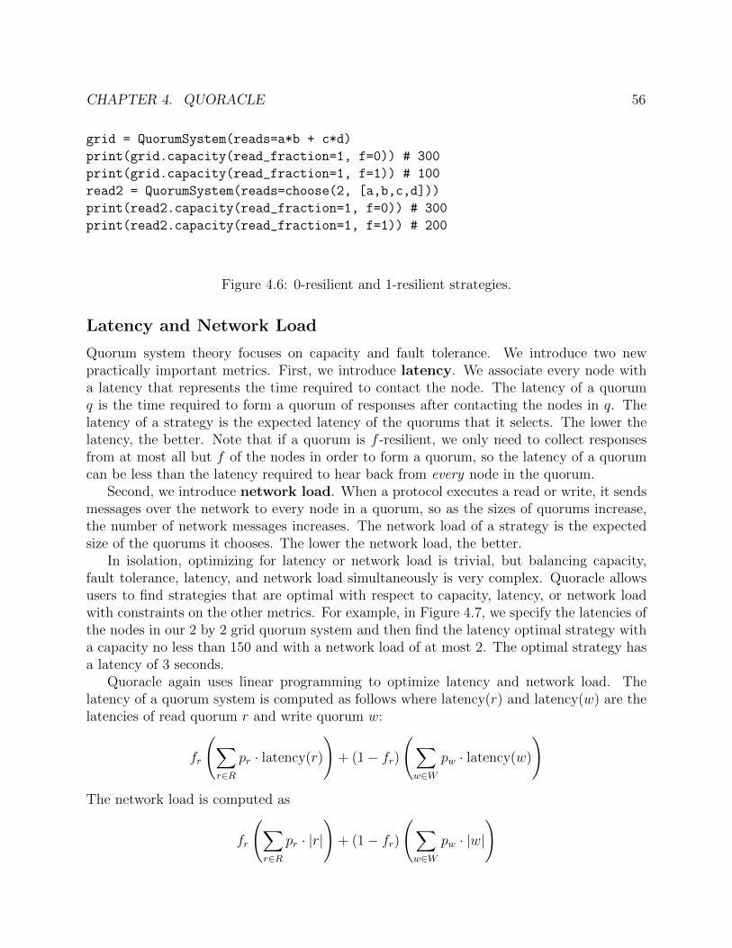
CHAPTER 4. QUORACLE 56
grid = QuorumSystem(reads=a*b + c*d)
print(grid.capacity(read_fraction=1, f=0)) # 300
print(grid.capacity(read_fraction=1, f=1)) # 100
read2 = QuorumSystem(reads=choose(2, [a,b,c,d]))
print(read2.capacity(read_fraction=1, f=0)) # 300
print(read2.capacity(read_fraction=1, f=1)) # 200
Figure 4.6: 0-resilient and 1-resilient strategies.
Latency and Network Load
Quorum system theory focuses on capacity and fault tolerance. We introduce two newpractically important metrics. First, we introduce latency. We associate every node witha latency that represents the time required to contact the node. The latency of a quorumq is the time required to form a quorum of responses after contacting the nodes in q. Thelatency of a strategy is the expected latency of the quorums that it selects. The lower thelatency, the better. Note that if a quorum is f -resilient, we only need to collect responsesfrom at most all but f of the nodes in order to form a quorum, so the latency of a quorumcan be less than the latency required to hear back from every node in the quorum.
Second, we introduce network load. When a protocol executes a read or write, it sendsmessages over the network to every node in a quorum, so as the sizes of quorums increase,the number of network messages increases. The network load of a strategy is the expectedsize of the quorums it chooses. The lower the network load, the better.
In isolation, optimizing for latency or network load is trivial, but balancing capacity,fault tolerance, latency, and network load simultaneously is very complex. Quoracle allowsusers to find strategies that are optimal with respect to capacity, latency, or network loadwith constraints on the other metrics. For example, in Figure 4.7, we specify the latencies ofthe nodes in our 2 by 2 grid quorum system and then find the latency optimal strategy witha capacity no less than 150 and with a network load of at most 2. The optimal strategy hasa latency of 3 seconds.
Quoracle again uses linear programming to optimize latency and network load. Thelatency of a quorum system is computed as follows where latency(r) and latency(w) are thelatencies of read quorum r and write quorum w:
fr
(∑r∈R
pr · latency(r)
)+ (1− fr)
(∑w∈W
pw · latency(w)
)The network load is computed as
fr
(∑r∈R
pr · |r|
)+ (1− fr)
(∑w∈W
pw · |w|
)

CHAPTER 4. QUORACLE 57
a = Node(’a’, write_cap=100, read_cap=200, latency=4)
b = Node(’b’, write_cap=100, read_cap=200, latency=4)
c = Node(’c’, write_cap=50, read_cap=100, latency=1)
d = Node(’d’, write_cap=50, read_cap=100, latency=1)
grid = QuorumSystem(reads=a*b + c*d)
sigma = grid.strategy(read_fraction = 1,
optimize = ’latency’,
capacity_limit = 150,
network_limit = 2)
print(sigma.latency(read_fraction=1)) # 3 seconds
Figure 4.7: Finding a latency-optimal strategy with capacity and network load constraints.
Note that in reality, the relationships between load, latency, and network load are com-plex. For example, as the load on a node increases, the latencies of the requests sent to itincrease. Moreover, the clients that communicate with the nodes in a quorum system mayexperience different latencies based on where they are physically located. We leave thesecomplexities to future work.
Quorum System Search
Thus far, we have demonstrated how Quoracle makes it easy to model, analyze, and optimizea specific hand-chosen quorum system. Quoracle also implements a heuristic based searchprocedure to find good quorum systems. For example, in Figure 4.8, we search for a quorumsystem over the nodes {a, b, c, d} optimized for latency with a capacity of at least 150 anda network load of at most 2. The search procedure returns the quorum system with readquorums a+ b+ c+ d and write quorums abcd, and with the read strategy that picks c onethird of the time and d two thirds of the time.
Given a list of expressions e = e1, . . . , en, let choose(k; e) be the disjunction of the con-junction of every set of k expressions in e. For example, choose(2; a, b, c) = ab + ac + bc,and choose(1; a, b, c) = a + b + c. Given a boolean expression e representing a set of quo-rums, we say e is duplicate free if e can be expressed using logical or, logical and, andchoose with every variable in e appearing exactly once. For example a + bc is duplicatefree. ab + ac = a(b + c) is duplicate free. ab + ac + bc = choose(2; a, b, c) is duplicate free.ab+ ace+ de+ dcb is not duplicate free.
Our search procedure exhaustively searches the space of all quorum systems that haveread quorums expressible by a duplicate free expression. The search procedure heuristicallyexplores simpler expressions first. Specifically, it enumerates expressions in increasing orderof their depth when represented as an abstract syntax tree. Because the search space isenormous, users can specify a timeout.

CHAPTER 4. QUORACLE 58
qs, sigma = search(nodes = [a, b, c, d],
read_fraction = 1,
optimize = ’latency’,
capacity_limit = 150,
network_limit = 2)
print(qs) # reads=a+b+c+d, writes=a*b*c*d
print(sigma) # c: 1/3, d: 2/3
print(sigma.latency(read_fraction=1)) # 1 second
print(sigma.capacity(read_fraction=1)) # 150
Figure 4.8: Searching the space of quorum systems.
4.3 Case Study
In this section, we present a hypothetical case study that demonstrates how to use Quoraclein a realistic setting. Assume we have five nodes. Nodes a, c, and e can process 2,000 writesper second, while nodes b and d can only process 1,000 writes per second. All nodes processreads twice as fast as writes. Nodes a and b have a latency of 1 second; nodes c, d, and ehave latencies of 3, 4, and 5 seconds. We observe a workload with roughly equal amounts ofreads and writes with a slight skew towards being read heavy. In Figure 4.9, we use Quoracleto model the nodes and workload distribution.
Assume we have already deployed a majority quorum system with a uniform strategy,which has a capacity of 2,292 commands per second. We want to find a more load optimalquorum system. We consider three candidates. The first is the majority quorum system.The second is a staggered grid quorum system, illustrated in Figure 4.10a. The third is aquorum system based on paths through a two-dimensional grid illustrated in Figure 4.10b.This quorum system has theoretically optimal capacity [64]. In Figure 4.11, we constructthese three quorum systems and print their capacities.
a = Node(’a’, write_cap=2000, read_cap=4000, latency=1)
b = Node(’b’, write_cap=1000, read_cap=2000, latency=1)
c = Node(’c’, write_cap=2000, read_cap=4000, latency=3)
d = Node(’d’, write_cap=1000, read_cap=2000, latency=4)
e = Node(’e’, write_cap=2000, read_cap=4000, latency=5)
fr = {0.9: 10/470, 0.8: 20/470, 0.7: 100/470,
0.6: 100/470, 0.5: 100/470, 0.4: 60/470,
0.3: 30/470, 0.2: 30/470, 0.1: 20/470}
Figure 4.9: Nodes and workload distribution.

CHAPTER 4. QUORACLE 59
a b
d e f
(a) Staggered grid quorum system
a bc
d e
(b) Paths quorum system
Figure 4.10: The read quorums of the staggered grid and paths quorum systems. The optimalset of complementary write quorums is chosen automatically.
maj = QuorumSystem(reads=majority([a, b, c, d, e]))
grid = QuorumSystem(reads=a*b + c*d*e)
paths = QuorumSystem(reads=a*b + a*c*e + d*e + d*c*b)
print(maj.capacity(reads_fraction=fr)) # 3,667
print(grid.capacity(reads_fraction=fr)) # 4,200
print(paths.capacity(reads_fraction=fr)) # 4,125
Figure 4.11: Quorum systems and their capacities.
The capacities are 3,667, 4,200, and 4,125 commands per second respectively, making thegrid quorum system the most attractive. However, the grid quorum system is not necessarilyoptimal. In Figure 4.12, we perform a search for a quorum system optimized for capacitythat is tolerant to one failure. The search takes 7 seconds on a laptop.
qs, sigma = search(nodes=[a, b, c, d, e],
fault_tolerance=1,
read_fraction=fr)
print(qs.capacity(read_fraction=fr)) # 5,005
Figure 4.12: Searching for a load-optimal quorum system.
The search procedure finds the quorum system with read quorums (c+bd)(a+e) which hasa capacity of 5,005 commands per second. This is 1.19× better than the grid quorum system,and 2.18× better than the majority quorum system with a naive uniform strategy. Assumehypothetically that we deploy this strategy to production. Months later, we introduce acomponent into our system that bottlenecks our throughput at 2,000 commands per second.Now, any capacity over 2,000 is wasted, so we search for a quorum system optimized forlatency with a capacity of at least 2,000. We again consider our three quorum systems inFigure 4.13.

CHAPTER 4. QUORACLE 60
for qs in [maj, grid, paths]:
print(qs.latency(read_fraction=fr,
optimize=’latency’,
capacity_limit=2000))
Figure 4.13: Latencies with a capacity constraint.
The quorum systems have latencies of 3.24, 1.95, and 2.43 seconds respectively, makingthe grid quorum system the most attractive. We again perform a search and find the quorumsystem with read quorums ab+acde+ bcde achieves a latency of 1.48 seconds. This is 1.32×better than the grid and 3.04× better than a naive uniform strategy over a majority quorumsystem. The search again completes in 7 seconds. We hypothetically deploy this quorumsystem to production.
4.4 Lessons Learned
Naive Majority Quorums Underperform
Industry practitioners often use majority quorums because they are simple and have strongfault tolerance. Our case study shows that majority quorum systems with uniform strate-gies almost always underperform more sophisticated quorum systems in terms of capacity,latency, and network load. In Figure 4.14, we plot a stacked histogram of the throughputthat every node in a majority quorum system obtains using a naive uniform strategy, withthroughput broken down by quorums. We contrast this in Figure 4.15 with the strategyfound in Figure 4.12. The sophisticated quorum system assigns more work to machines withhigher capacities, leading to a 2.18× increase in aggregate throughput. Moreover, the per-formance benefits of more sophisticated quorum systems do not sacrifice correctness, unlikealternatives like sloppy quorums [19].
“Optimal” Is Not Always Best.
There is a large body of research on constructing “optimal” quorum systems [24, 56, 2,39, 16, 64, 70]. For example, the paths quorum system is theoretically optimal, but in ourcase study, it has lower capacity and higher latency than the simpler grid quorum system.There are two reasons for this mismatch between theoretical and practical optimality. First,existing quorum system theory does not account for node heterogeneity and workload skew.Second, these quorum systems are only optimal in the limit, as the number of nodes tendsto infinity.

CHAPTER 4. QUORACLE 61
a b c d eNode
0
250
500
750
1000
1250
Thro
ughp
ut(c
omm
ands
per
seco
nd)
abc abc abcabd abd
abdabe abe
abe
acdacd acd
aceace
ace
ade
ade adebcd bcd bcdbce bce
bcebde
bde bdecde cde cde
abc abc abcabd abd
abdabe abe
abe
acdacd acd
aceace
ace
ade
ade adebcd bcd bcdbce bce
bcebde
bde bdecde cde cde
Figure 4.14: A stacked histogram of the throughput of a simple majority quorum systemwith a naive uniform strategy. Write quorums are in blue, and read quorums are in red.
a b c d eNode
0
1000
2000
Thro
ughp
ut(c
omm
ands
per
seco
nd)
ac ac
ce
cebde bdebde
bc
bccd
cd
ae ae
Figure 4.15: A stacked histogram of the throughput of the quorum system found by ourheuristic search (i.e., the quorum system with read quorums (c+ bd)(a+ e)).
The Trade-Off Space Is Complex
Constructing a quorum system of homogeneous nodes that is optimal in the limit for a fixedworkload is difficult but doable. When nodes operate at different speeds and workloadsskew, finding an optimal quorum system that satisfies constraints on capacity, fault toler-ance, latency, and network load becomes nearly impossible to do by hand. Moreover, smallperturbations in any of these parameters can change the landscape of the optimal quorumsystems. In our case study, for example, the search procedure finds two different quorumsystems when optimizing for load and when optimizing for latency. We believe that using anautomated assistance library like ours is the only realistic way to find good quorum systems.

62
Chapter 5
Bipartisan Paxos
In Chapter 3, we saw how to use compartmentalization to make state machine replicationprotocols faster without making them more complicated. Now, we show how to use compart-mentalization to make complicated state machine replication protocols easier to understandwithout making them slower.
There is a family of generalized multi-leader state machine replication protocols, includingEPaxos [62], Caesar [6], and Atlas [21]. These protocols are multi-leader, which means thatthey have multiple simultaneous leaders. This avoids having a single bottlenecked leader.They are also generalized [42, 55], which means that every replica executes non-commutingcommands in the exact same order, but are otherwise free to execute commuting commandsin any order. In other words, these protocols execute a partially ordered graph of commandsrather than a totally ordered log of commands.
These generalized multi-leader protocols are extremely complicated. Paxos has a wellknown reputation for being complex [44, 87, 68], and these generalized multi-leader protocolsare significantly more complex than that. They require a strong understanding of moresophisticated Paxos variants like Fast Paxos [41] and are overall less intuitive and morenuanced. It is hard to measure this complexity precisely, but there are indications that theprotocols are complicated. EPaxos, for example, had several bugs go undiscovered for yearsdespite the popularity of the protocol [81].
This complexity has negative consequences in industry and academia. Generalized multi-leader protocols have little to no industry adoption. We postulate that this is largely due totheir complexity. The engineers in [12] explain that implementing a state machine replicationprotocol requires making many small changes to the protocol to match the environment inwhich it is deployed. Making these changes without a strong understanding of the protocol isinfeasible. Academically, it is challenging to understand the novelty of each protocol becausethe protocols have not been cleanly factored. The protocols are all very similar, yet they alsohave lots of small differences between them, some novel and some inconsequential. Withouta clean factoring of the protocols’ designs, it is difficult to understand where each protocolis novel. This makes it difficult to extend the protocols with further innovations, as it isunclear which ideas have already been explored and which have yet to be examined.

CHAPTER 5. BIPARTISAN PAXOS 63
In this chapter, we use compartmentalization as a tool to understand these protocols.Rather than presenting a monolithic, nuanced, and highly optimized protocol, we present afully compartmentalized and completely unoptimized generalized multi-leader protocol thatis designed to be simple to understand. We then slowly reassemble the components andintroduce optimizations to recreate existing protocols like EPaxos, Caesar, and Atlas. Indoing so, we create a framework for understanding generalized multi-leader protocols.
The tutorial has four parts, and in each part, we introduce a new protocol. First, wepresent a fully compartmentalized generalized multi-leader protocol, which we called SimpleBPaxos (Section 5.2). Simple BPaxos sacrifices performance for simplicity and is designedwith the sole goal of being easy to understand. Simple BPaxos is the kernel from which allother generalized multi-leader protocols can be constructed. It encapsulates all the mecha-nisms and invariants that are common to the other protocols.
Second, we introduce a purely pedagogical protocol called Fast BPaxos (Section 5.4).Fast BPaxos achieves higher performance than Simple BPaxos, but it is unsafe. The protocoldoes not properly implement state machine replication. Why study a broken protocol?Because understanding why Fast BPaxos does not work leads to a fundamental insight onwhy other protocols do. Specifically, we discover that generalized multi-leader protocolsencounter a fundamental tension between agreeing on commands and ordering commands.In isolation, reaching consensus on what command to execute is easy, and determining howthe command should be ordered with respect to other commands is easy, but doing both atthe same time is hard. This is where the tension arises. The way in which a protocol handlesthis tension is its key distinguishing feature. We taxonomize the protocols into those thatavoid the tension and those that resolve the tension.
Third, we introduce Unanimous BPaxos, a simple tension avoiding protocol (Sec-tion 5.5). We describe how tension avoiding protocols carefully enlarge quorum sizes tosidestep the tension. We also explain how Basic EPaxos [62] and Atlas [21] can be expressedas optimized variants of Unanimous BPaxos.
Fourth, we introduce Majority Commit BPaxos, a tension resolving protocol (Sec-tion 5.6). We describe how tension resolving protocols perform detective work to resolve thetension without enlarging quorum sizes. We also discuss the relationship between MajorityCommit BPaxos and the tension resolving protocols EPaxos [60] and Caesar [6]. A full tax-onomy of these protocols and other related protocols is shown in Figure 5.13 at the end ofthis chapter.
5.1 Conflict Graphs
Defining Conflict Graphs
By totally ordering state machine commands into a log, state machine replication protocolslike MultiPaxos ensure that every replica executes every command in exactly the same order.This is a simple way to ensure that replicas are always in sync, but it is sometimes unnec-

CHAPTER 5. BIPARTISAN PAXOS 64
essary [42]. For example, consider the log shown at the top of Figure 5.1. The commanda=2 (i.e. set the value of variable a to 2) is chosen in log entry 1, and the command b=1 ischosen in log entry 2. With MultiPaxos, every replica would execute these two commands inexactly the same order, but this is not necessary because the commands commute. It is safefor some replicas to execute a=2 before b=1 while other replicas execute b=1 before a=2. Theexecution order of the two commands has no effect on the final state of the state machine,so they can be safely reordered, as shown in Figure 5.1.
x
0
a=2
1
b=1
2
y
3
b=1
2
z
4
· · ·
x
0
b=1
1
a=2
2
y
3
a=2
2
z
4
· · ·
Figure 5.1: If two commands commute, replicas can safely execute them in either order.
More formally, we say two commands x and y conflict if there exists a state in whichexecuting x and then y does not produce the same responses or final state as executing yand then x. We say two commands commute if they do not conflict. If two commandsconflict (e.g., a=1 and a=2), then they need to be executed by every state machine replica inthe same order. But, if two commands commute (e.g., a=2 and b=1), then they do not needto be totally ordered. State machine replicas can execute them in either order.
Generalized Multi-leader state machine replication protocols like EPaxos, Caesar, Atlas,and all the BPaxos variants presented in this chapter take advantage of command commu-tativity. Rather than totally ordering commands into a log, these protocols partially ordercommands into a directed graph such that every pair of conflicting commands has an edgebetween them. We call these graphs conflict graphs. An example log and correspondingconflict graph is illustrated in Figure 5.2. A log consists of a number log entries, and everylog entry has a unique log index (e.g., 4). A conflict graph consists of a number of vertices,and every vertex has a unique vertex id (e.g., v4).
Moreover, a vertex v can have directed edges to other vertices. These are called thedependencies of v, denoted deps(v). For example, if vertex vi depends on vertex vj, thenthere is an edge from vi to vj. Note that if a pair of commands conflict, then they musthave an edge between them. This ensures that every replica executes the two commands inthe same order. For example in Figure 5.2, the commands a=b (v0) and a=2 (v1) conflict,so they have an edge between them. If two commands commute, then they do not havean edge between them. This allows replicas to execute the commands in either oder. Forexample, the commands a=2 (v1) and b=1 (v2) commute, so there is no edge between them.Finally note that some conflicting commands (e.g., b=a (v3) and a=3 (v4)) have edges in

CHAPTER 5. BIPARTISAN PAXOS 65
a=b
0
a=2
1
b=1
2
b=a
3
a=3
4
(a)
a=bv0
a=2v1
b=1v2
b=av3
a=3v4
(b)
Figure 5.2: A log and corresponding conflict graph.
both directions, forming a cycle. Ideally, conflict graphs would be acyclic, but cycles aresometimes unavoidable. The reason for this will become clear soon.
Executing Conflict Graphs
We now explain how to execute a static conflict graph. In the next subsection, we explainhow to execute a dynamic conflict graph that grows over time. Replicas execute logs inprefix order. Replicas execute conflict graphs in reverse topological order, one strongly con-nected component at a time. The order of executing commands within a strongly connectedcomponent is not important, but every replica must choose the same order. For example,replicas can execute commands within a component sorted by their vertex id. The conflictgraph in Figure 5.2 has four strongly connected components, each shaded a different color.Vertices v0, v1, and v2 are each in their own components, and commands v3 and v4 are intheir own component. Replicas execute these four strongly connected components in reversetopological order as follows:
• First, replicas execute a=b (v0).
• Next, replicas either execute a=2 (v1) then b=1 (v2) or b=1 (v2) then a=2 (v1). Thereare no edges between vertex v1 and vertex v2, so every replica can execute the twovertices in either order.
• Finally, replicas execute b=a (v3) and a=3 (v4) in some arbitrary but fixed order. Forexample, if replicas execute commands sorted by their vertex ids, then the replicaswould all execute v3 and then v4.
Executing commands in this way, state machine replicas are guaranteed to remain in sync.Every replica executes conflicting commands in the same order, but are free to executecommuting commands in any order.

CHAPTER 5. BIPARTISAN PAXOS 66
a=bv0
(a)
a=bv0
a=2v1
(b)
a=bv0
a=2v1
v2
b=av3 v4
(c)
a=bv0
a=2v1
b=1v2
b=av3 v4
(d)
a=bv0
a=2v1
b=1v2
b=av3
a=3v4
(e)
a=b
0
(f)
a=b
0
a=2
1
(g)
a=b
0
a=2
1 2
b=a
3
(h)
a=b
0
a=2
1
b=1
2
b=a
3
b=1
2
(i)
a=b
0
a=2
1
b=1
2
b=a
3
a=3
4
(j)
Figure 5.3: In subfigures (a) - (e), we see a conflict graph constructed over time. Themost recently chosen vertex is drawn in red. The executed commands are shaded green.(a) The command a=b is chosen in vertex v0 without any dependencies. The command isexecuted immediately. (b) The command a=2 is chosen in vertex v1 with a dependency onv0. The command is executed immediately. (c) The command b=a is chosen in vertex v3with dependencies on v0, v1, v2, and v4. No commands have been chosen in v2 and v4 yet,so v3 cannot be executed. (d) The command b=1 is chosen in vertex v2 with a dependencyon v0. The command is executed immediately. (e) The command a=3 is chosen in vertex v4with dependencies on v0, v1, and v3. Now v3 and v4 are executed. In subfigures (f) - (j), wesee an analogous execution for a log.
Constructing Conflict Graphs
In the previous subsection, we explained how to execute a static conflict graph. In reality,graphs are dynamic and grow over time. MultiPaxos constructs one log entry at a time. Ituses one instance of consensus for every log entry i to choose which command should beplaced in log entry i. Analogously, generalized multi-leader protocols construct a conflictgraph one vertex at a time. They use one instance of consensus for every vertex v to choosewhich command should be placed in vertex v and what dependencies, or outbound edges, vshould have.
In Figure 5.3, we illustrate an example execution of how the conflict graph from Figure 5.2could be constructed over time. Figure 5.3 also shows an analogous execution in which alog is constructed over time. Note that a vertex v can be chosen with dependencies deps(v)before every vertex in deps(v) has itself been chosen. For example in Figure 5.3c, v3 is chosenwith deps(v3) = {v0, v1, v2, v4} before vertices v2 and v4 are chosen. This is analogous to howa command is chosen in log entry 3 in Figure 5.3h before a command is chosen in entry 2.
A summary of the differences between logs and graphs is given in Table 5.1.

CHAPTER 5. BIPARTISAN PAXOS 67
Table 5.1: The differences between protocols like MultiPaxos and Raft that organize com-mands in logs and protocols like EPaxos, Caesar, and Atlas that organize commands ingraphs.
Logs Graphs
data structure log conflict graphlog entry vertexlog index (e.g., 4) vertex id (e.g., v4)total order partial order
execution order log order reverse topological orderwhat’s chosen? commands commands & dependencies
Two Key Invariants
Protocols like EPaxos, Caesar, Atlas, and the BPaxos protocols in this chapter all differ inhow they assign commands to vertices, how they compute dependencies, how they implementconsensus, and so on. Despite the differences, all the protocols construct conflict graphs onevertex at a time, choosing a command and a set of dependencies (x, deps(v)) for every vertexv. The protocols all rely on the following two key invariants for correctness. We call thesethe consensus invariant (Invariant 1) and the dependency invariant (Invariant 2).
Invariant 1 (Consensus Invariant). Consensus is implemented for every vertex v. That is,at most one value (x, deps(v)) is chosen for every vertex v.
Invariant 2 (Dependency Invariant). If (x, deps(vx)) is chosen in vertex vx and (y, deps(vy))is chosen in instance vy, and if x and y conflict, then either vx ∈ deps(vy) or vy ∈ deps(vx)or both. That is, if two chosen commands conflict, there is an edge between them.
The consensus invariant ensures that replicas always agree on the state of the conflictgraph. It makes it impossible, for example, for two replicas to disagree on which commandis in a vertex or disagree on what dependencies a vertex has. The dependency invariantensures that replicas execute conflicting commands in the same order but does not requirethat replicas execute commuting commands in the same order. These two invariants aresufficient to ensure linearizable execution. Intuitively, the history of command executionis equivalent to a serial history following any reverse topological ordering of the conflictgraph. In fact, replicas literally do execute commands serially according to one of the reversetopological orderings. For a more formal proof, refer to [42] and [60].

CHAPTER 5. BIPARTISAN PAXOS 68
5.2 Simple BPaxos
In this section, we introduce Simple BPaxos, an inefficient protocol that is designed tobe easy to understand. By understanding Simple BPaxos, we will understand of the coremechanisms and invariants that are common to all generalized multi-leader protocols.
Overview
c1
c2
p1 p2
d1 d2 d3 a1 a2 a3
r1 r2
Clients
f + 1Proposers
2f + 1Dependency Service
Nodes2f + 1
Acceptors
f + 1Replicas
1
2 2 23 3 3 4 4 45 5 5
6 67
Figure 5.4: An example execution of Simple BPaxos (f = 1).
As illustrated in Figure 5.4, a Simple BPaxos deployment consists of a number of clients,a set of at least f + 1 Paxos proposers, a set of 2f + 1 dependency service nodes, a set of2f + 1 Paxos acceptors, and a set of at least f + 1 replicas. These nodes have the followingresponsibilities.
• The dependency service nodes, collectively called the dependency service, computedependencies and maintain the dependency invariant (Invariant 2).
• The proposers and acceptors implement one instance of Paxos for every vertex andmaintain the consensus invariant (Invariant 1).
• The replicas construct and execute conflict graphs and send the results of executingcommands back to the clients.

CHAPTER 5. BIPARTISAN PAXOS 69
More concretely, Simple BPaxos executes as follows. The numbers here correspond tothe numbered arrows in Figure 5.4.
• (1) When a client wants to propose a state machine command x, it sends x to any ofthe proposers. Note that with MultiPaxos, only one proposer is elected leader, but inSimple BPaxos, every proposer is a leader.
• (2) and (3) When a proposer pi receives a command x, from a client, it places xin a vertex with globally unique vertex id vx = (pi,m) where m is a monotonicallyincreasing integer local to pi. For example, proposer pi places the first command thatit receives in vertex (pi, 0), the next command in vertex (pi, 1), the next in (pi, 2), andso on. The proposer then performs a round trip of communication with the dependencyservice. It sends vx and x to the dependency service, and the dependency service replieswith the dependencies deps(vx). For now, we leave this process abstract. We’ll explainhow the dependency service computes dependencies in Section 5.2.
• (4) and (5) The proposer pi then executes Phase 2 of Paxos with the acceptors,proposing that the value (x, deps(vx)) be chosen in the instance of Paxos associatedwith vertex vx = (pi,m). This is analogous to a MultiPaxos leader running Phase 2,proposing the command x be chosen in the instance of Paxos associated with log entrym.
Recall from Section 2.2 that the Paxos proposer executing round 0 can safely bypassPhase 1. By design, we predetermine that the proposer pi leads round 0 for vertices ofthe form (pi,m). This is why pi can safely bypass Phase 1 and immediately executePhase 2.
In the normal case, pi gets the value (x, deps(vx)) chosen in vertex vx. It is also possiblethat some other proposer erroneously concluded that pi had failed and proposed someother value in vertex vx, but we discuss this scenario later.
• (6) The proposer pi broadcasts vx, x, and deps(vx) to all of the replicas. The replicasadd vertex vx to their conflict graph with command x and with edges to the verticesin deps(vx). The replicas execute their conflict graphs as described in Section 5.1.
• (7) Once a replica executes command x, it sends the result of executing command xback to the client.
Dependency Service
The dependency service consists of 2f + 1 dependency service nodes d1, . . . , d2f+1. Everydependency service node maintains an acyclic conflict graph. These conflict graphs aresimilar but not equal to the conflict graph that Simple BPaxos ultimately executes.
When a proposer sends a vertex vx with command x to the dependency service, it sendsvx and x to every dependency service node. When a dependency service node di receives vx

CHAPTER 5. BIPARTISAN PAXOS 70
wvw
(a) wvw
x
vx
(b)
wvw
x
vx
yvy
(c)
wvw
x
vx
yvy
z vz
(d)
wvw
x
vx
yvy
z vz
(e)
Figure 5.5: In subfigures (a) – (e), we see the execution of a dependency service node di. (a) direceives command w in vertex vw. di adds this vertex to its conflict graph and because thereare no other vertices, it returns the dependencies deps(vw) = ∅. (b) di receives command xin vertex vx. di adds this vertex to its conflict graph. x conflicts with w, so di adds an edgefrom vx to vw and returns the dependencies deps(vx) = {vw}. (c) di receives command y invertex vy. di adds this vertex to its conflict graph. y conflicts with w and x, so di adds anedge from vy to vw and from vy to vx. It returns the dependencies deps(vy) = {vw, vx}. (d)di receives command z in vertex vz. di adds this vertex to its conflict graph. z conflicts withw and x, so di adds an edge from vz to vw and from vz to vx. It returns the dependenciesdeps(vz) = {vw, vx}. (e) di receives command x in vertex vx. di’s graph already containsvertex vx, so di returns the dependencies deps(vx) = {vw} and does not modify its graph.
and x, it performs one of the following two actions depending on whether di’s graph alreadycontains vertex vx.
• If di’s conflict graph does not contain vertex vx, then di adds vertex vx to its graphwith command x. di adds an edge from vx to every other vertex vy with command yif x and y conflict. Letting out(vx) be the set of vertices to which vx has an edge, dithen returns out(vx) to the proposer.
• Otherwise, if di’s conflict graph already contains vertex vx, then di does not modify itsconflict graph. It immediately returns out(vx) to the proposer.
An example execution of a dependency service node is given in Figure 5.5.When a proposer receives replies from f + 1 dependency service nodes, it takes the union
of these responses as the value of deps(vx). For example, imagine f = 1 and a proposerreceives dependencies {vw, vy} from d1 and dependencies {vw, vz} from d2. The proposercomputes deps(vx) = {vw, vy, vz}. The dependency service maintains Invariant 3.
Invariant 3. If two conflicting commands x and y in vertices vx and vy yield dependenciesdeps(vx) and deps(vy) from the dependency service, then either vx ∈ deps(vy) or vy ∈deps(vx) or both.

CHAPTER 5. BIPARTISAN PAXOS 71
Proof. Consider conflicting commands x and y in vertices vx and vy with dependenciesdeps(vx) and deps(vy) computed by the dependency service. deps(vx) is the union of depen-dencies computed by f + 1 dependency service nodes Dx. Similarly, deps(vy) is the union ofdependencies computed by f + 1 dependency service nodes Dy. Because f + 1 is a majorityof 2f + 1, Dx and Dy necessarily intersect. That is, there is some dependency service nodedi that is in Dx and Dy. di either received vx or vy first. If it received vx first, then it returnsvx as a dependency of vy, so vx ∈ deps(vy). If it received vy first, then it returns vy as adependency of vx, so vy ∈ deps(vx).
Note that the dependency service may process a vertex more than once, yielding differ-ent dependencies each time. For example, a proposer may sent vx and x to the dependencyservice and get back dependencies {vw, vy}. The proposer might resend vx and x to thedependency service and get a different set of dependencies {vy, vz}. Even though the de-pendency service may compute different dependencies for the same vertex, the dependencyservice still maintains Invariant 3 for every possible pair of computed dependencies.
An Example
An example execution of Simple BPaxos with f = 1 is illustrated in Figure 5.6.
• In Figure 5.6a, proposer p1 receives command x from a client, while proposer p2 receivescommand y from a client. The commands are placed in vertices vx and vy respectively.
• In Figure 5.6b, p1 sends x in vx to the dependency service, while p2 concurrently sendsy in vy. Dependency service nodes d1 and d2 receive x and then y, so they computedeps(vx) = ∅ and deps(vy) = {vx}. d3, on the other hand, receives y and then x andcomputes deps(vx) = {vy} and deps(vy) = ∅p1 receives ∅ from d2 and {vy} from d3. Two dependency service nodes form a majority,so p1 computes deps(vx) = {vy} ∪ ∅ = {vy}. Similarly, p2 receives {vx} from d2 and∅ from d3, so p2 computes deps(vy) = {vx} ∪ ∅ = {vx}. Note that p1 and p2 alsoreceive responses from d1, but proposers form dependencies from the first set of f + 1dependency service nodes they hear from.
• In Figure 5.6c, p1 executes Phase 2 of Paxos to get the value (x, {vy}) chosen in vertexvx. p2 likewise gets the value (y, {vx}) chosen in vertex vy.
• In Figure 5.6d, the proposers broadcast their commands to the replicas. The replicasadd vx and vy to their conflict graphs and execute the commands once they havereceived both. One or more of the replicas also sends the results of executing x and yback to the clients.
Note that the replicas’ conflict graphs contain a cycle. This is because the dependencyservice nodes do not receive every command in the same order. In Figure 5.6, dependencyservice nodes d2 and d3 receive x and y in opposite orders, leading to the two commands

CHAPTER 5. BIPARTISAN PAXOS 72
d1 d2 d3
p1p2
a1
a2
a3
r1 r2
xy
(a) p1 receives command x; p2 receivescommand y.
d1 d2 d3
p1p2
a1
a2
a3
r1 r2
xvx
yvy
xvx
yvy
xvx
yvy
(b) The proposers contact the dependencyservice.
d1 d2 d3
p1p2
a1
a2
a3
r1 r2
xvx
yvy
xvx
yvy
xvx
yvy
(c) The proposers contact the acceptors.
d1 d2 d3
p1p2
a1
a2
a3
r1 r2
xvx
yvy
xvx
yvy
xvx
yvy
xvx
yvy
xvx
yvy
(d) The proposers notify the replicas.
Figure 5.6: An example execution of Simple BPaxos (f = 1).
depending on each other. It is tempting to enforce that every dependency service node receiveevery command in exactly the same order, but unfortunately, this would be tantamount tosolving consensus [12].

CHAPTER 5. BIPARTISAN PAXOS 73
d1 d2 d3
p1p2
a1
a2
a3
r1 r2
x
xvx
xvx
xvx
(a) p1 receives x, talks to the dependencyservice, and fails.
d1 d2 d3
p1p2
a1
a2
a3
r1 r2
xvx
yvy
xvx
yvy
xvx
yvy
vx
yvy
vx
yvy
y
(b) p2 receives y, gets it chosen with adependency on vx.
d1 d2 d3
p1p2
a1
a2
a3
r1 r2
xvx
yvy
xvx
yvy
xvx
yvy
vx
yvy
vx
yvy
(c) A replica notifies p2 that vx is uncho-sen.
d1 d2 d3
p1p2
a1
a2
a3
r1 r2
xvx
yvy
xvx
yvy
xvx
yvy
noopvx
yvy
noopvx
yvy
(d) p2 gets a noop chosen in vx.
Figure 5.7: An example execution of Simple BPaxos recovery (f = 1).
Recovery
Imagine a proposer receives a command x from a client, places the command x in vertex vx,sends vx and x to the dependency service, and then crashes. Because a command and a set ofdependencies have not been chosen in vertex vx yet, we call vx unchosen. It is possible that acommand y chosen in vertex vy depends on an unchosen vertex vx. If vertex vx remains forever

CHAPTER 5. BIPARTISAN PAXOS 74
unchosen, then the command y will never be executed. To avoid this liveness violation, ifany replica notices that vertex vx has been unchosen for some time, it notifies a proposer.The proposer then executes Phase 1 and Phase 2 of Paxos with the acceptors to get a noopchosen in vertex vx without any dependencies. noop is a distinguished command that doesnot affect the state machine and does not conflict with any other command. An example ofthis execution is given in Figure 5.7.
• In Figure 5.7a, proposer p1 receives command x from a client. It places x in vertex vxand sends vx and x to the dependency service. Shortly after, it fails.
• In Figure 5.7b, proposer p2 receives command y from a client. It places y in vy andcontacts the dependency service. The dependency service nodes have already receivedx in vx, so they compute deps(vy) = {vx}. p2 then gets y chosen in vertex vy with adependency on vx and broadcasts it to the replicas.
• In Figure 5.7c, the replicas cannot execute vertex vy because it depends on the unchosenvertex vx. After a timeout expires, replica r1 notifies p2 that the vertex has beenunchosen for some time.
• In Figure 5.7d, p2 executes Phase 1 and Phase 2 of Paxos in some round r > 0 with theacceptors to get the command noop chosen in vertex vx without any dependencies. p2notifies the replicas, and the replicas place the noop in vertex vx. The replicas executetheir conflict graphs in reverse topological order. They execute the noop first (whichhas no effect) and then execute y.
Note that p2 must execute both phases of Paxos because it is not in round 0. This isnecessary to ensure that no other value could have been chosen in vx.
Note that a Simple BPaxos proposer recovers a command and proposes a noop by exe-cuting Paxos as normal. Simple BPaxos does not require an additional recovery protocol.Rather, commands and noops are proposed in the exact same way. This simplifies theprotocol.
Safety
To ensure that Simple BPaxos is safe, we must ensure that it maintains the consensusinvariant and the dependency invariant. Simple BPaxos maintains the consensus invariantbecause it implements Paxos. The dependency invariant follows immediately from Invariant 3and the fact that noops don’t conflict with any other command.
Practical Considerations
We discuss a few practical considerations that are important when implementing SimpleBPaxos and the other BPaxos variants in this chapter.

CHAPTER 5. BIPARTISAN PAXOS 75
Ensuring Exactly Once Semantics If a client proposes a command but does not hearback quickly enough, it re-proposes the command to make sure that the command eventuallygets executed. Thus, Simple BPaxos might receive a command more than once, but it hasto guarantee that it never executes the command more than once. Executing a commandmore than once would violate exactly once semantics.
Non-generalized protocols like MultiPaxos [87], Viewstamped Replication [53], and Raft [68]all employ the following technique to avoid executing a command more than once. First,before a client proposes a command to a replication protocol, it annotates the commandwith a monotonically increasing integer-valued id. Moreover, clients only send one commandat a time, waiting to receive a response from one command before sending another. Second,every replica maintains a client table, like the one illustrated below. A client table has oneentry per client. The entry for a client records the largest id of any command that the replicahas executed for that client, along with the result of executing the command with that id.A replica only executes commands for a client if it has a larger id than the one recorded inthe client table. If it receives a command with the same id as the one in the client table, itreplies with the recorded output instead of executing the command a second time.
Client Id Output10.31.14.41 2 “foo”10.54.13.123 1 “bar”
Naively applying this same trick to Simple BPaxos (or any generalized protocol) is unsafe.For example, imagine a client issues command x with id 1. The command gets chosen andis executed by replica 1. Then, the client issues non-conflicting command y with id 2. Thecommand gets chosen and is executed by replica 2. Because y has a larger id than x, replica2 will never execute x.
To fix this bug, a replica must record the ids of all commands that it has executed for aclient, along with the output corresponding to the largest of these ids. Replicas only executecommands they have not previously executed, and relay the cached output if they receive acommand with the corresponding id.
Dependency Compaction Upon receiving a command x in vertex vx, a dependencyservice node returns the set of all previously received vertices with commands that conflictwith x. Over time, as the dependency service receives more and more commands, thesedependency sets get bigger and bigger. As the dependency sets get bigger, Simple BPaxos’throughput decreases because more time is spent sending these large dependency sets, andless time is spent doing useful work.
To combat this, a dependency service node has to compact dependencies in some way.Recall that proposer pi creates vertex ids (pi, 0), (pi, 1), (pi, 2), and so on. Thus, vertex idsacross all the leaders form a two-dimensional array with one column for every leader indexand one row for every monotonically increasing id.

CHAPTER 5. BIPARTISAN PAXOS 76
b d
a e
c
p0 p1 p2
0
1
2
3
proposer
id
Figure 5.8: An example of dependency compaction
For example, consider a dependency service node that has received commands a, b, c, d,and e in vertices (p0, 1), (p0, 0), (p1, 2), (p1, 0), and (p2, 1) as shown in Figure 5.8. Withoutdependency compaction, if the dependency service node receives a command that conflictswith commands a, b, c, d, and e, it would return the vertex ids of these five commands.In our example, the dependency service node returns only five dependencies, but in a realdeployment, the node could return hundreds of thousands of dependencies.
With dependency compaction on the other hand, the dependency service node insteadartificially adds more dependencies. In particular, for every proposer pi, it computes thelargest id j for which a dependency (pi, j) exists. Then, it adds {(pi, k) | k ≤ j} to thedependencies. In other words, it finds the largest dependency in each column and then addsall of the vertex ids below it as dependencies. In Figure 5.8, the inflated set of dependenciesis highlighted in blue. Even though more dependencies have been added, the set of inflateddependencies can be represented more compactly, with a single integer for every leader (i.e.,the id of the largest command for that leader). Thus, every BPaxos dependency set can besuccinctly represented with n integers (for n proposers).
Scaling Following the design pattern of compartmentalization, we can scale up each com-ponent of Simple BPaxos because the protocol is fully decoupled. We could introduce proxyleaders, but because Simple BPaxos is a multi-leader protocol, there is no need. Instead, wecan scale up the number of proposers directly. We can scale up the acceptors using acceptorgrids or any other read-write quorum system. We can scale up the dependency service usingan arbitrary quorum system, as the dependency service’s correctness only relies on intersect-ing quorums. Note that we use a quorum system—a system in which every pair of quorumsintersect—rather than a read-write quorum system. We can also scale up the number ofreplicas to reduce the number of replies the replicas have to send to the clients.
An interesting phenomenon happens when we fully scale up Simple BPaxos. The onlycomponent of the protocol that is not scalable is the replicas executing writes. Every replicahas to execute every write no matter what. Executing writes is bottlenecked on executing theconflict graphs in reverse topological order. This process is significantly slower than executingcommands in a simple log. This means that without compartmentalization, generalized

CHAPTER 5. BIPARTISAN PAXOS 77
multi-leader protocols are often faster than simpler log-based protocols like MultiPaxos.But, after compartmentalization, the simpler log-based protocols are faster. Generalizedprotocols introduced graphs as a way to avoid bottlenecks, but after compartmentalization,the graphs become the bottlenecks.
5.3 Fast Paxos
Algorithm 3 Fast Paxos Proposer
State: a value v, initially nullState: a round i, initially −11: upon receiving Phase2B〈0, v′〉 from f + maj(f + 1)
acceptors as the proposer of round 0 with i = 0 do2: if every value of v′ is the same then3: v′ is chosen, notify the learners4: else5: i← 16: proceed to line 11 viewing every Phase2B〈0, v′〉
as a Phase1B〈1, 0, v′〉7: upon recovery do8: i← next largest round owned by this proposer9: send Phase1A〈i〉 to the acceptors
10: upon receiving Phase1B〈i, vr, vv〉 from f + 1 acceptors do11: k ← the largest vr in any Phase1B〈i, vr, vv〉12: if k = −1 then13: v ← an arbitrary value14: else if k > 0 then15: v ← the corresponding vv in round k16: else if k = 0 then17: if there are maj(f + 1) Phase1B〈i, 0, v′〉
messages for some value v′ then18: v ← v′
19: else20: v ← an arbitrary value
21: send Phase2A〈i, v〉 to the acceptors
22: upon receiving Phase2B〈i〉 from f + 1 acceptors do23: v is chosen, notify the learners
Simple BPaxos is designed to be easy to understand, but as shown in Figure 5.6, it takesseven network delays (in the best case) between when a client proposes a command x and

CHAPTER 5. BIPARTISAN PAXOS 78
Algorithm 4 Fast Paxos Acceptor
State: the largest seen round r, initially −1State: the largest round vr voted in, initially −1State: the value vv voted for in round vr, initially null1: upon receiving value v from client do2: if r = −1 then3: r, vr, vv ← 0, 0, v4: send Phase2B〈0, v〉 to proposer of round 0
5: upon receiving Phase1A〈i〉 from p with i > r do6: r ← i7: send Phase1B〈i, vr, vv〉 to p
8: upon receiving Phase2A〈i, v〉 from p with i ≥ r do9: r, vr, vv ← i, i, v10: send Phase2B〈i〉 to p
when a client receives the result of executing x. Call this duration of time the commit time.Generalized multi-leader protocols like EPaxos, Caesar, and Atlas all achieve a commit timeof only four network delays in the best case. They do so by leveraging Fast Paxos [41].
Fast Paxos is a Paxos variant that allows clients to propose values directly to the acceptorswithout having to initially contact a proposer. Fast Paxos is an optimistic protocol. If allof the acceptors happen to receive the same command from the clients, then Fast Paxoshas a commit time of only three network delays. This is called the fast path. However, ifmultiple clients concurrently propose different commands, and not all of the acceptors receivethe same command, then the protocol reverts to a slow path and introduces two additionalnetwork delays to the commit time. In this section, we review a slightly simplified versionof Fast Paxos.
Overview
Like Paxos, a Fast Paxos deployment consists of some number of clients, f + 1 proposers,and 2f + 1 acceptors. We also include a set of f + 1 learners. These nodes are notifiedof the value chosen by Fast Paxos. Note that we use the term learner rather than replicabecause Fast Paxos is a consensus protocol and not a state machine replication protocol, sothere are no state machine replicas. A Fast Paxos deployment is illustrated in Figure 5.9.Proposer and acceptor pseudocode are given in Algorithm 3 and Algorithm 4.
Like Paxos, Fast Paxos is divided into a number of integer valued rounds. The keydifference is that round 0 of Fast Paxos is a special “fast round.” A client can propose avalue directly to an acceptor in round 0 without having to contact a proposer first. Thenormal case execution of Fast Paxos is illustrated in Figure 5.9a. The execution proceeds asfollows:

CHAPTER 5. BIPARTISAN PAXOS 79
p1
p2
p3
a1
a2
a3
a4
a5
l1
l2
l3
f + 1Proposers
2f + 1Acceptors
f + 1Learners
1
1
1
1
2
2
2
2
3
3
3
(a) Normal case execution.
p1
p2
p3
a1
a2
a3
a4
a5
l1
l2
l3
f + 1Proposers
2f + 1Acceptors
f + 1Learners
1
1
1
2
2
2
3
3
3
4
4
4
5
5
5
(b) Recovery.
p1
p2
p3
a1
a2
a3
a4
a5
l1
l2
l3
f + 1Proposers
2f + 1Acceptors
f + 1Learners
1
1
1
1
2
2
2
2
3
3
3
4
4
4
5
5
5
(c) Coordinated recovery.
Figure 5.9: Example executions of Fast Paxos (f = 2). The leader of round 0 is adornedwith a crown. Client requests are drawn in red. Phase 1 messages are drawn in blue. Phase2 messages are drawn in green.
• (1) When a client wants to propose a value v, it sends v to all of the acceptors.
• (2) When an acceptor receives a value v from a client, the acceptor ignores v if it hasalready received a message in some round i ≥ 0. Otherwise, it votes for v by updatingits state and sending a Phase2B〈0, v〉 message to the proposer that leads round 0.This is shown in Algorithm 4 line 1 – line 4.
• (3) Let maj(n) = dn+12e be a majority of n. If the proposer that leads round 0 receives
Phase2B〈0, v′〉 messages from f +maj(f + 1) acceptors for the same value v′, then v′
is chosen, and the proposer notifies the learners. This is shown in Algorithm 3 line 1– line 3. We consider what happens when not every value is the same in Section 5.3.
Recovery
Note that in Paxos, a value is chosen when f + 1 acceptors vote for it in some round i. Inround 0 of Fast Paxos, a value is chosen when f+maj(f+1) acceptors vote for it. The largernumber of required votes is needed to ensure the safety of recovery, which we now describe.

CHAPTER 5. BIPARTISAN PAXOS 80
Let p be the proposer leading round 0. Recovery is the process by which a proposer otherthan p gets a value chosen. For example, if p fails, some other proposer must take over andget a value chosen. Recovery is illustrated in Figure 5.9b.
• (1) and (2) A recovering proposer performs Phase 1 of Paxos with at least f + 1acceptors in some round i > 0. This is shown in Algorithm 3 line 7 – line 9 andAlgorithm 4 line 5 – line 7.
• (3) and (4) The recovering proposer receives Phase1B〈i, vr, vv〉 messages from f +1acceptors. Call this quorum of acceptors A. The proposer computes k as the largestreceived vr (line 11). This is the largest round in which any acceptor in A has voted.If k = −1 (line 12), then none of the acceptors have voted in any round less than i,so the proposer is free to propose an arbitrary value. This is the same as in Paxos.If k > 0 (line 14), then the proposer must propose the value vv proposed in roundk. Again, this is the same as in Paxos. vv may have been chosen in round k, so theproposer is forced to propose it as well. If k = 0 (line 16), then there are two cases toconsider.
First, if maj(f + 1) of the acceptors in A have all voted for some value v′ in round 0,then it’s possible that v′ was chosen in round 0 (line 17). Specifically, if all f of theacceptors not in A voted for v′ in round 0, then along with the maj(f + 1) of acceptorsin A who also voted for v′ in round 0, there is a quorum of f+maj(f+1) acceptors whovoted for v′ in round 0. In this case, the proposer must propose v′ as well since it mighthave been chosen. Second, if there does not exist maj(f + 1) votes for any value v′,then the proposer concludes that no value was chosen or every will be chosen in round0, so it is free to propose an arbitrary value (line 19). Once the recovering proposerdetermines which value to propose, it gets the value chosen with the acceptors usingthe normal Phase 2 of Paxos.
Note that a value must receive at least f + maj(f + 1) votes in round 0 to be chosen.If this number were any smaller, it would be possible for a recovering proposer to findtwo distinct values v′ and v′′ that both could have been chosen in round 0. In this case,the proposer cannot make progress. It cannot propose v′ because v′′ might have beenchosen, and it cannot propose v′′ because v′ might have been chosen
More concretely, imagine an Fast Paxos deployment with f = 2 and five acceptors a1,a2, . . ., a5. Further imagine that a value is considered chosen after receiving votes fromonly 3 (i.e. f + 1) acceptors rather than the correct number of 4 (i.e. f + maj(f + 1)).Consider a proposer executing Phase 1 in round 1. It contacts a3, a4, and a5. a3 votedfor value x in round 0; a4 voted for value y in round 0; and a5 didn’t vote in round0. What value should the proposer propose in Phase 2? Well, x was maybe chosen inround 0 (if a1 and a2 both voted for x in round 0), so the proposer has to propose x.However, y was also maybe chosen in round 0 (if a1 and a2 both voted for y in round0), so the proposer also has to propose y. The proposer can only propose one value,

CHAPTER 5. BIPARTISAN PAXOS 81
so the protocol gets stuck. By requiring f + maj(f + 1) votes rather than f + 1 votes,we eliminate these situations. It’s not possible for two values to both potentially havereceived f + maj(f + 1) votes. There isn’t enough acceptors for this to be possible.
• (5) The proposer notifies the learners of the chosen value.
Coordinated Recovery
Finally, we consider what happens when the proposer of round 0 receives f + maj(f + 1)Phase1B messages from the acceptors, but without all of them containing the same valuev′. Naively, the proposer could simply perform a recovery, executing both phases of Paxos issome round r > 0. However, if we assign rounds to proposers in such a way that the proposerof round 0 is also the proposer of round 1, then we can take advantage of an optimizationcalled coordinated recovery. This is illustrated in Figure 5.9c and proceeds as follows:
• (1) Multiple clients send distinct commands directly to the acceptors.
• (2) The acceptors receive and vote for the commands and send Phase2B messagesto the leader of round 0. However, not every acceptor receives the same value first, sonot all the acceptors vote for the same value.
• (3) and (4) The proposer receives Phase2B messages from f +maj(f + 1) acceptors,but the acceptors have not all voted for the same value. At this point, the proposercould naively perform a recovery in round 1 by executing Phase 1 and then Phase 2 ofPaxos. But, executing Phase 1 in round 1 is redundant, since the Phase2B messagesin round 0 contain exactly the same information as the Phase1B messages in round1. Specifically, the proposer can view every Phase2B〈0, v′〉 message as a proxy for aPhase1B〈1, 0, v′〉 message. Thus, the proposer instead jumps immediately to Phase2 in round 1 to get a value chosen (line 4 – line 6).
• (5) Finally, the proposer notifies the learners of the chosen value.
5.4 Fast BPaxos
In this section, we present a purely pedagogical protocol called Fast BPaxos. Fast BPaxosachieves a commit time of four network delays (compared to Simple BPaxos’ seven), butFast BPaxos is unsafe. It does not properly implement state machine replication. To un-derstand why more complex protocols like EPaxos, Caesar, and Atlas work the way theydo, it helps to understand why simpler protocols like Fast BPaxos don’t work in the firstplace. Understanding why Fast BPaxos is unsafe leads to fundamental insights into theseother protocols.

CHAPTER 5. BIPARTISAN PAXOS 82
c1
c2
d1 d2 d3
a1 a2 a3
p1 p2 p3
r1 r2 r3
Clients
2f + 1 Dependency
Service Nodes
2f + 1 Acceptors
2f + 1 Proposers
2f + 1 Replicas
Server 1 Server 2 Server 3
1
2 2
23 3 3
4 4 4
5 5 56
Figure 5.10: An example execution of Fast BPaxos (f = 1). The four network delays aredrawn in red.
The Protocol
Fast BPaxos is largely identical to Simple BPaxos with one key observation. Rather thanimplementing Paxos, Fast BPaxos implements Fast Paxos. This allows the protocol to reducethe commit time by overlapping communication with the dependency service (to computedependencies) and communication with the acceptors (to implement consensus).
As shown in Figure 5.10, a Fast BPaxos deployment consists of 2f+1 dependency servicenodes, 2f + 1 Fast Paxos acceptors, 2f + 1 Fast Paxos proposers, and 2f + 1 replicas. Theselogical nodes are co-located on a set of 2f + 1 servers, where every physical server executesone dependency service node, one acceptor, one proposer, and one replica. For example, inFigure 5.10, server 2 executes d2, a2, p2, and r2. As illustrated in Figure 5.10, the protocolexecutes as follows:
• (1) When a client wants to propose a state machine command x, it sends x to any ofthe proposers.
• (2) When a proposer pi receives a command x, from a client, it places x in a vertexwith globally unique vertex id vx = (pi,m) where m is a monotonically increasinginteger local to pi. pi then sends vx and x to all of the dependency service nodes. Notethat we predetermine that proposer pi is the leader of round 0 and 1 of the Fast Paxosinstance associated with vertex vx = (pi,m).
• (3) When a dependency service node dj receives a command x in vertex vx, it com-putes a set of dependencies deps(vx) in the exact same way as in Simple BPaxos (i.e. djmaintains an acyclic conflict graph). Unlike Simple BPaxos however, dj does not send

CHAPTER 5. BIPARTISAN PAXOS 83
deps(vx) back to the proposer. Instead, it proposes to the co-located Fast Paxos accep-tor aj that the value (x, deps(vx)) be chosen in the instance of Fast Paxos associatedwith vertex vx in round 0.
• (4) Fast BPaxos acceptors are unmodified Fast Paxos acceptors. In the normal case,when an acceptor aj receives value (x, deps(vx)) in vertex vx = (pi,m), it votes for thevalue and sends the vote to pi.
• (5) Fast BPaxos proposers are unmodified Fast Paxos proposers. In the normal case,pi receives f + maj(f + 1) votes for value (x, deps(vx)) in vertex vx, so (x, deps(vx)) ischosen. The proposer broadcasts the command and dependencies to the replicas. Ifpi receives f + maj(f + 1) votes, but they are not all for the same value, the proposerexecutes coordinate recovery (see Algorithm 3 line 4 – line 6).
• (6) Fast BPaxos replicas are identical to Simple BPaxos replicas. Replicas maintainand execute conflict graphs, returning the results of executing commands to the clients.
Note that Figure 5.10 illustrates six steps of execution, but the commit time is onlyfour network delays (drawn in red). Communication between co-located components (e.g.,between d1 and a1 and between p1 and r1) does not involve the network and therefore doesnot contribute to the commit time.
Recovery
As with Simple BPaxos, it is possible that a command y chosen in vertex vy depends on anunchosen vertex vx that must be recovered for execution to proceed. Fast BPaxos performsrecovery in the same way as Simple BPaxos. If a replica detects that a vertex vx has beenunchosen for some time, it notifies a proposer. The proposer then executes a Fast Paxosrecovery to get a noop chosen in vertex vx with no dependencies.
Lack of Safety
We now demonstrate why Fast BPaxos is unsafe. Consider the execution of Fast BPaxos(f = 2) illustrated in Figure 5.11.
• In Figure 5.11a, proposer p1 receives command x from a client. It places x in vertexvx and sends vx and x to the dependency service. d1 and d2 receive the message. Theyplace x in their conflict graphs without any dependencies, and send the value (x, ∅) totheir co-located acceptors. a1 and a2 vote for (x, ∅) in vertex vx, but p1 crashes beforeit receives any of these votes. The messages sent to d3, d4, and d5 are dropped by thenetwork.
• Similarly in Figure 5.11a, proposer p5 receives a conflicting command y, p5 sends vyand y to d4 and d5, d4 and d5 propose (y, ∅) to a4 and a5, a4 and a5 vote for theproposed values, and p5 fails.

CHAPTER 5. BIPARTISAN PAXOS 84
d1 d2 d3 d4 d5
a1 a2 a3 a4 a5
p1 p2 p3 p4 p5
r1 r2 r3 r4 r5
x y
xvx
xvx
yvy
yvy
(a) p1 receives x, talks to the dependencyservice, and fails. p2 receives y, talks to thedependency service, and fails.
d1 d2 d3 d4 d5
a1 a2 a3 a4 a5
p1 p2 p3 p4 p5
r1 r2 r3 r4 r5
xvx
xvx
yvy
yvy
xvx
yvy
xvx
yvy
xvx
yvy
xvx
yvy
xvx
yvy
(b) p2 recovers vx with command x and nodependencies. p4 recovers vy with commandy and no dependencies.
Figure 5.11: A Fast BPaxos bug (f = 2). Conflicting commands x and y are executed indifferent orders by different replicas.
• In Figure 5.11b, p2 recovers vertex vx. To recover vx, p2 executes Phase 1 of Fast Paxoswith acceptors a1, a2, and a3. p2 observes that a1 and a2 both voted for the value (x, ∅)in round 0. Therefore, p2 concludes that (x, ∅) may have been chosen in round 0, so itproceeds to Phase 2 and gets the value (x, ∅) chosen in vertex vx (Algorithm 3 line 17).p2 cannot propose any other value (e.g., a noop) because (x, ∅) may have already beenchosen. From our omniscient view of the execution, we know that (x, ∅) was neverchosen, but from p2’s myopic view, it cannot make this determination and so is forcedto propose (x, ∅). This is a critical point in the execution, which we will discussfurther in a moment.
• In Figure 5.11b, proposer p4 recovers vertex vy in much the same way as p2 recoversvx. p4 observes that a4 and a5 voted for (y, ∅) in round 0, so it is forced to get thevalue (y, ∅) chosen.
• Finally in Figure 5.11b, proposers p2 and p4 broadcast (x, ∅) and (y, ∅) to all of thereplicas. The replicas place x and y in their conflict graphs without edges betweenthem. This violates the dependency invariant. x and y conflict, so there must be anedge between them. Without an edge, the replicas can execute x and y in differentorders, causing their states to diverge.
What went wrong? When p2 was recovering vx, Fast Paxos forced it to choose (x, ∅).However, the dependencies deps(vx) = ∅ were not computed by a majority of the dependency

CHAPTER 5. BIPARTISAN PAXOS 85
service nodes. They were computed only by d1 and d2. This is what allowed conflictingcommands x and y to be chosen without a dependency on each other.
This example illustrates a fundamental tension between preserving the consensus in-variant (Invariant 1) and preserving the dependency invariant (Invariant 2). Maintaining theconsensus invariant in isolation is easy (e.g., use Paxos), and maintaining the dependencyinvariant in isolation is also easy (e.g., use the dependency service). But, maintaining bothinvariants simultaneously is tricky.
When performing a recovery, like the one in our example above, a proposer is sometimesforced to propose a particular value (e.g., (x, ∅)) in order to properly implement consensusand simultaneously forced not to propose the value in order to correctly compute depen-dencies. Resolving the tension between the consensus and dependency invariants duringrecovery is the single most important and the single most challenging aspect of generalizedmulti-leader protocols like EPaxos, Caesar, and Atlas. All of these protocols have a similarstructure and execution on the normal path. They all compute dependencies from a ma-jority of servers, and they all execute Fast Paxos variants to get these dependencies chosen.If you understand the normal case execution of one of these protocols, it is not difficult tounderstand the others. The key feature that distinguishes the protocols is how they resolvethe fundamental tension between implementing consensus and computing dependencies.
These protocols all take different approaches to resolving the tension. In the next twosections, we broadly categorize the approaches into two main techniques: tension avoidanceand tension resolution. Tension avoidance involves cleverly manipulating quorum sizes toavoid the tension entirely. This approach is used by Basic EPaxos [60] and Atlas [21]. Thesecond technique, tension resolution, is significantly more complicated and involves detectingand resolving the tension through various means.
5.5 Tension Avoidance
In this section, we explain how to implement a generalized multi-leader state machine repli-cation protocol using tension avoidance. The key idea behind tension avoidance is toavoid the tension between the consensus and dependency invariants entirely. By manipu-lating quorum sizes in clever ways, we can ensure that whenever a proposer is forced topropose a set of dependencies deps(vx), this set of dependencies is guaranteed to satisfy thedependency invariant.
We first introduce Unanimous BPaxos, a simple protocol that implements tension avoid-ance. We then explain how Basic EPaxos and Atlas can be expressed as two optimizedvariants of Unanimous BPaxos.
Unanimous BPaxos
A Fast BPaxos deployment consists of 2f + 1 servers. A proposer communicates with f + 1acceptors in Phase 1 called a Phase 1 quorum, f + maj(f + 1) acceptors in Phase 2 of

CHAPTER 5. BIPARTISAN PAXOS 86
round 0 called a fast Phase 2 quorum, and f + 1 acceptors in Phase 2 of rounds greaterthan 0 called a classic Phase 2 quorum. If we adjust the sizes of these quorums, we canavoid the tension between implementing consensus and computing dependencies. In [30],Howard et. al prove that Fast Paxos is safe so long as the following two conditions are met.
1. Every Phase 1 quorum and every classic Phase 2 quorum intersect. That is, for everyPhase 1 quorum Q and for every classic Phase 2 quorum Q′, Q ∩Q′ 6= ∅.
2. Every Phase 1 quorum and every pair of fast Phase 2 quorums intersect. That is, forevery Phase 1 quorum Q and for every pair of fast Phase 2 quorum Q′, Q′′, Q∩Q′∩Q′′ 6=∅.
Unanimous BPaxos takes advantage of this result and increases the size of fast Phase 2quorums. Specifically, Unanimous BPaxos is identical to Fast BPaxos except with fast Phase2 quorums of size 2f + 1. Unanimous BPaxos proposer pseudocode is given in Algorithm 5.It is identical to the pseudocode of a Fast Paxos proposer (Algorithm 3) except for a couplesmall changes highlighted in red.
Unlike Fast BPaxos, Unanimous BPaxos is safe. The critical change is on line 18. Withfast Phase 2 quorums of size 2f +1 (line 1), a recovering proposer knows that a value v′ mayhave been chosen in round 0 only if all f + 1 acceptors that it communicates with in Phase1 voted for v′ in round 0. If even a single acceptor did not vote for v′ in round 0, then v′
could not have received a unanimous vote and therefore was not chosen in round 0.With Fast BPaxos, a proposer executing line 17 of Algorithm 3 is forced to propose a
value (x, deps(vx)) if maj(f + 1) acceptors voted for it in round 0, but the dependenciesdeps(vx) may have only been computed by maj(f + 1) dependency service nodes, violatingthe dependency invariant. This is exactly what happened in Figure 5.11. Unanimous BPaxosavoids the tension entirely because a proposer is only forced to propose a value (x, deps(vx))if f+1 acceptors voted for it in round 0. Now, we are guaranteed that deps(vx) was computedby a majority (i.e. f + 1) of the dependency service nodes. Thus, Unanimous BPaxos safelymaintains the consensus and dependency service invariants.
The obvious disadvantage of Unanimous BPaxos is the protocol’s large quorum sizes. Inorder to get a command chosen, a proposer has to perform a round trip of communicationwith every acceptor. This not only slows down the protocol in the normal case, it alsodecreases the protocol’s ability to remain live in the face of faults. If even a single acceptorfails, the protocol grinds to a halt. This problem can be partially fixed by using more flexiblequorums (like what Atlas [21] does) or by using a tension resolving protocol (see Section 5.5).
We now present two independent optimizations that improve the performance of Unani-mous BPaxos. These optimizations were introduced in EPaxos [62] and Atlas [21].
Basic EPaxos Optimization
Unanimous BPaxos has a lower commit time than Simple BPaxos (4 network delays insteadof 7), but has larger fast Phase 2 quorums (2f + 1 acceptors instead of f + 1). We now

CHAPTER 5. BIPARTISAN PAXOS 87
Algorithm 5 Unanimous BPaxos Proposer. Changes to Algorithm 3 are highlighted in red.
State: a value v, initially nullState: a round i, initially −11: upon receiving Phase2B〈0, v′〉 from all 2f + 1
acceptors as the proposer of round 0 with i = 0 do2: if every value of v′ is the same then3: v′ is chosen, notify the learners4: else5: i← 16: v ← an arbitrary value satisfying the dependency
invariant7: send Phase2A〈i, v〉 to the acceptors
8: upon recovery do9: i← next largest round owned by this proposer10: send Phase1A〈i〉 to the acceptors
11: upon receiving Phase1B〈i, vr, vv〉 from f + 1 acceptors do12: k ← the largest vr in any Phase1B〈i, vr, vv〉13: if k = −1 then14: v ← an arbitrary value satisfying the dependency
invariant15: else if k > 0 then16: v ← the corresponding vv in round k17: else if k = 0 then18: if all f + 1 messages are of the form
Phase1B〈i, 0, v′〉 for some value v′ then19: v ← v′
20: else21: v ← an arbitrary value satisfying the
dependency invariant
22: send Phase2A〈i, v〉 to the acceptors
23: upon receiving Phase2B〈i〉 from f + 1 acceptors do24: v is chosen, notify the learners
discuss an optimization, used by Basic EPaxos [62], to reduce the fast Phase 2 quorum sizeto 2f .
An execution of Unanimous BPaxos with the Basic EPaxos optimization is shown inFigure 5.12. We walk through the execution, highlighting the optimization’s key changes.We assume f > 1 for now. Later, we discuss the case when f = 1.
• (1) When a client wants to propose a state machine command x, it sends x to any of

CHAPTER 5. BIPARTISAN PAXOS 88
d1
a1
p1
r1
d2
a2
p2
r2
d3
a3
p3
r3
d4
a4
p4
r4
d5
a5
p5
r5
c1
c2
Server 1 Server 2 Server 3 Server 4 Server 5
1
2
3 3 3 3
4 4 4 4 4
55 5 5 5
6 7
8 8 8 8 89
Figure 5.12: An example execution of Unanimous BPaxos (f = 2) with the Basic EPaxosoptimization. The messages introduced by the optimization are drawn in red.
the proposers.
• (2) When a proposer pi receives a command x, from a client, it places x in a vertexwith globally unique vertex id vx = (pi,m). Change: pi then sends vx and x to theco-located dependency service node di. It does not yet communicate with the otherdependency service nodes.
• (3) Change: When di receives vx and x, it computes the dependencies deps(vx)i asusual using its acyclic conflict graph. di then sends vx, x, and deps(vx)i to all the otherdependency service nodes.
• (4) When a dependency service node dj receives vx, x, and deps(vx)i, it computesthe dependencies deps(vx)j as usual using its acyclic conflict graph. Change: Then,dj proposes to its co-located acceptor aj that the value (x, deps(vx)i ∪ deps(vx)j) bechosen in vertex vx in round 0. dj combines the dependencies that it computed withthe dependencies computed by di.
• (5) The acceptors are unchanged. In the normal case, when an acceptor aj receivesvalue (x, deps(vx)) in vertex vx = (pi,m), it votes for the value and sends the vote topi.
• (6) and (7) Change: In Unanimous BPaxos, a value v = (x, deps(vx)) is consideredchosen in round 0 if all 2f + 1 acceptors vote for v in round 0. With the Basic EPaxosoptimization, we only require 2f votes, and the act of choosing a value in round 0 is
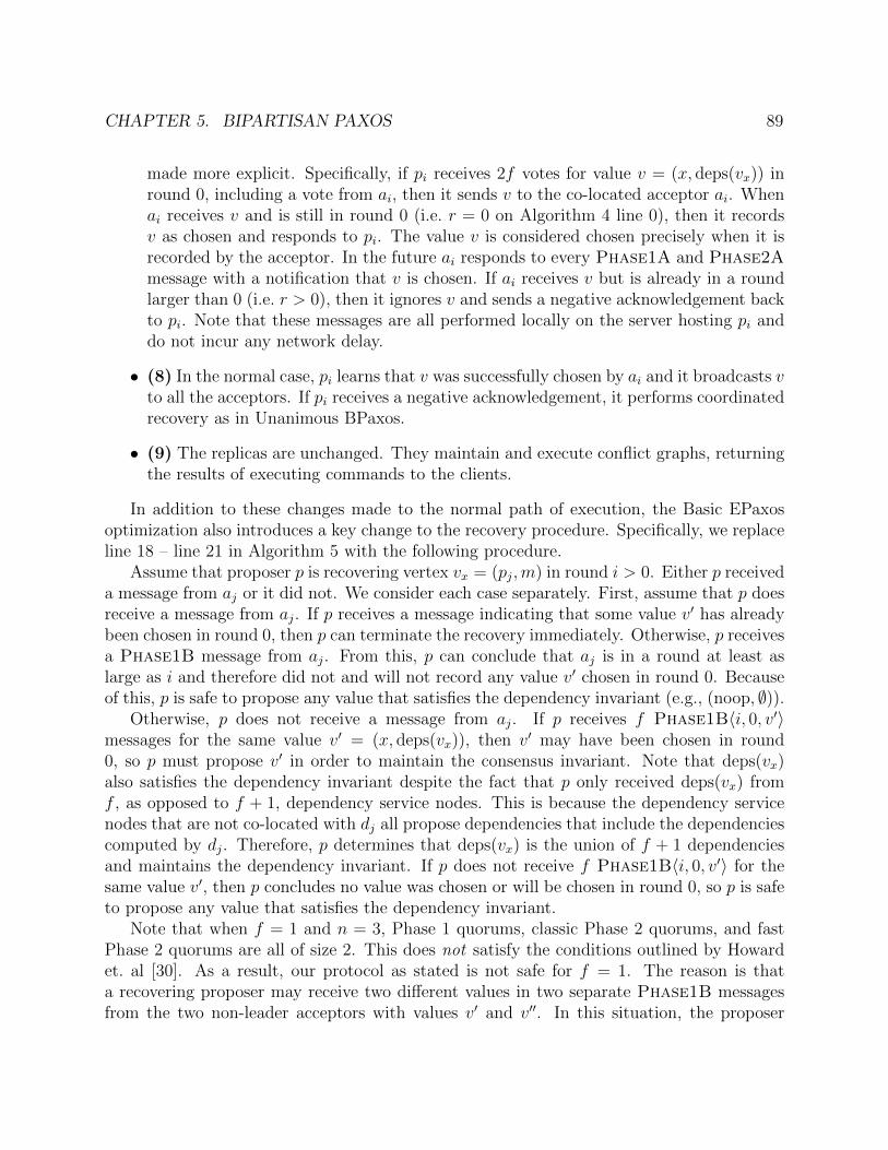
CHAPTER 5. BIPARTISAN PAXOS 89
made more explicit. Specifically, if pi receives 2f votes for value v = (x, deps(vx)) inround 0, including a vote from ai, then it sends v to the co-located acceptor ai. Whenai receives v and is still in round 0 (i.e. r = 0 on Algorithm 4 line 0), then it recordsv as chosen and responds to pi. The value v is considered chosen precisely when it isrecorded by the acceptor. In the future ai responds to every Phase1A and Phase2Amessage with a notification that v is chosen. If ai receives v but is already in a roundlarger than 0 (i.e. r > 0), then it ignores v and sends a negative acknowledgement backto pi. Note that these messages are all performed locally on the server hosting pi anddo not incur any network delay.
• (8) In the normal case, pi learns that v was successfully chosen by ai and it broadcasts vto all the acceptors. If pi receives a negative acknowledgement, it performs coordinatedrecovery as in Unanimous BPaxos.
• (9) The replicas are unchanged. They maintain and execute conflict graphs, returningthe results of executing commands to the clients.
In addition to these changes made to the normal path of execution, the Basic EPaxosoptimization also introduces a key change to the recovery procedure. Specifically, we replaceline 18 – line 21 in Algorithm 5 with the following procedure.
Assume that proposer p is recovering vertex vx = (pj,m) in round i > 0. Either p receiveda message from aj or it did not. We consider each case separately. First, assume that p doesreceive a message from aj. If p receives a message indicating that some value v′ has alreadybeen chosen in round 0, then p can terminate the recovery immediately. Otherwise, p receivesa Phase1B message from aj. From this, p can conclude that aj is in a round at least aslarge as i and therefore did not and will not record any value v′ chosen in round 0. Becauseof this, p is safe to propose any value that satisfies the dependency invariant (e.g., (noop, ∅)).
Otherwise, p does not receive a message from aj. If p receives f Phase1B〈i, 0, v′〉messages for the same value v′ = (x, deps(vx)), then v′ may have been chosen in round0, so p must propose v′ in order to maintain the consensus invariant. Note that deps(vx)also satisfies the dependency invariant despite the fact that p only received deps(vx) fromf , as opposed to f + 1, dependency service nodes. This is because the dependency servicenodes that are not co-located with dj all propose dependencies that include the dependenciescomputed by dj. Therefore, p determines that deps(vx) is the union of f + 1 dependenciesand maintains the dependency invariant. If p does not receive f Phase1B〈i, 0, v′〉 for thesame value v′, then p concludes no value was chosen or will be chosen in round 0, so p is safeto propose any value that satisfies the dependency invariant.
Note that when f = 1 and n = 3, Phase 1 quorums, classic Phase 2 quorums, and fastPhase 2 quorums are all of size 2. This does not satisfy the conditions outlined by Howardet. al [30]. As a result, our protocol as stated is not safe for f = 1. The reason is thata recovering proposer may receive two different values in two separate Phase1B messagesfrom the two non-leader acceptors with values v′ and v′′. In this situation, the proposer

CHAPTER 5. BIPARTISAN PAXOS 90
is unable to determine which value to propose. Thankfully, we can avoid this situation byhaving the leader send only to 2f acceptors rather than to all 2f + 1 acceptors.
Ignoring some minor cosmetic differences, Unanimous BPaxos with the Basic EPaxosoptimization is roughly equivalent to Basic EPaxos [62].
Atlas Optimization
In the best case, also called the fast path, Unanimous BPaxos achieves a commit time offour network delays. As shown in line 2 of Algorithm 5, a proposer executes the fast pathonly when every single acceptor votes for the exact same set of dependencies. As we saw inFigure 5.11, if any two dependency service nodes receive conflicting commands in differentorders, their computed dependencies will not be the same. If a proposer does not receive aunanimous vote, it executes coordinated recovery, adding two more network delays to thecommit time.
Atlas [21] introduces the following optimization to relax the requirement of a unanimousvote and increase the probability of a proposer executing the fast path. Let X1, . . . , X2f+1
be 2f + 1 sets. Let popular(X1, . . . , X2f+1) = {x |x appears in at least f + 1 of the sets}.We change line 2 as follows. When a proposer receives dependencies deps(vx)1, . . .,
deps(vx)2f+1 from the 2f+1 acceptors, it executes the fast path with dependencies deps(vx) =deps(vx)1∪· · ·∪deps(vx)2f+1 if deps(vx) = popular(deps(vx)1, . . . , deps(vx)2f+1). That is, theproposer takes the fast path only if every dependency vy computed by any of the dependencyservice nodes was computed by a majority of the dependency service nodes.
We also simplify line 18 – line 21. If a recovering proposer receives f + 1 sets of de-pendencies, it proposes their union. Otherwise, it proposes an arbitrary value. This is safebecause a set of dependencies deps(vx) can be chosen in round 0, only if every dependencyin deps(vx) was computed by a majority of the dependency service nodes. Thus, every suchelement will appear in at least one of the f + 1 dependency sets. Thus, the recoveringproposer is sure to propose a dependency set if it was previously chosen (maintaining theconsensus invariant), and it also proposes the union of f + 1 dependency sets (maintainingthe dependency invariant).
Atlas [21] is roughly equivalent to Unanimous BPaxos with the Basic EPaxos optimiza-tion, the Atlas optimization, and the flexible constraints on quorum sizes outlined in [30].
5.6 Tension Resolution
The advantage of tension avoidance is that it is simple. The disadvantage is that it requireslarge fast Phase 2 quorums. In this section, we explain how to implement a generalized multi-leader state machine replication protocol using tension resolution. Tension resolution issignificantly more complicated than tension avoidance, but it does not require large fastPhase 2 quorums.
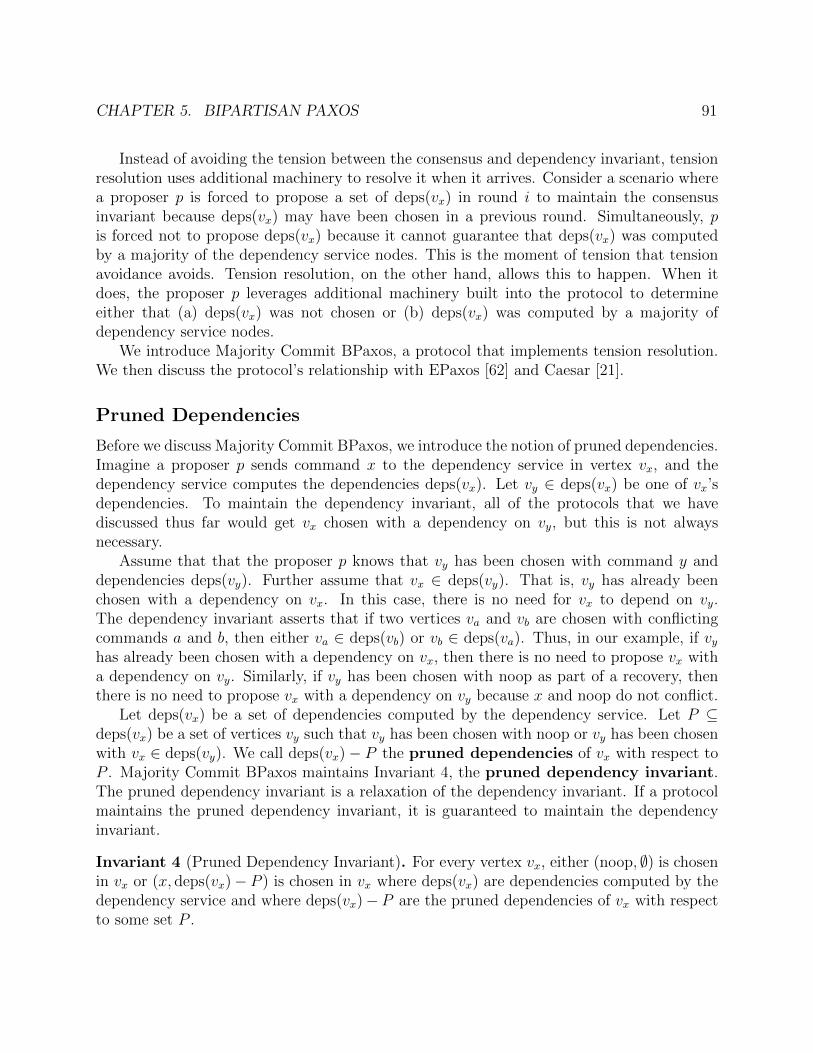
CHAPTER 5. BIPARTISAN PAXOS 91
Instead of avoiding the tension between the consensus and dependency invariant, tensionresolution uses additional machinery to resolve it when it arrives. Consider a scenario wherea proposer p is forced to propose a set of deps(vx) in round i to maintain the consensusinvariant because deps(vx) may have been chosen in a previous round. Simultaneously, pis forced not to propose deps(vx) because it cannot guarantee that deps(vx) was computedby a majority of the dependency service nodes. This is the moment of tension that tensionavoidance avoids. Tension resolution, on the other hand, allows this to happen. When itdoes, the proposer p leverages additional machinery built into the protocol to determineeither that (a) deps(vx) was not chosen or (b) deps(vx) was computed by a majority ofdependency service nodes.
We introduce Majority Commit BPaxos, a protocol that implements tension resolution.We then discuss the protocol’s relationship with EPaxos [62] and Caesar [21].
Pruned Dependencies
Before we discuss Majority Commit BPaxos, we introduce the notion of pruned dependencies.Imagine a proposer p sends command x to the dependency service in vertex vx, and thedependency service computes the dependencies deps(vx). Let vy ∈ deps(vx) be one of vx’sdependencies. To maintain the dependency invariant, all of the protocols that we havediscussed thus far would get vx chosen with a dependency on vy, but this is not alwaysnecessary.
Assume that that the proposer p knows that vy has been chosen with command y anddependencies deps(vy). Further assume that vx ∈ deps(vy). That is, vy has already beenchosen with a dependency on vx. In this case, there is no need for vx to depend on vy.The dependency invariant asserts that if two vertices va and vb are chosen with conflictingcommands a and b, then either va ∈ deps(vb) or vb ∈ deps(va). Thus, in our example, if vyhas already been chosen with a dependency on vx, then there is no need to propose vx witha dependency on vy. Similarly, if vy has been chosen with noop as part of a recovery, thenthere is no need to propose vx with a dependency on vy because x and noop do not conflict.
Let deps(vx) be a set of dependencies computed by the dependency service. Let P ⊆deps(vx) be a set of vertices vy such that vy has been chosen with noop or vy has been chosenwith vx ∈ deps(vy). We call deps(vx)− P the pruned dependencies of vx with respect toP . Majority Commit BPaxos maintains Invariant 4, the pruned dependency invariant.The pruned dependency invariant is a relaxation of the dependency invariant. If a protocolmaintains the pruned dependency invariant, it is guaranteed to maintain the dependencyinvariant.
Invariant 4 (Pruned Dependency Invariant). For every vertex vx, either (noop, ∅) is chosenin vx or (x, deps(vx)− P ) is chosen in vx where deps(vx) are dependencies computed by thedependency service and where deps(vx)− P are the pruned dependencies of vx with respectto some set P .

CHAPTER 5. BIPARTISAN PAXOS 92
Majority Commit BPaxos
For clarity of exposition, we first introduce a version of Majority Commit BPaxos that cansometimes deadlock. Later, we modify the protocol to eliminate the possibility of deadlock.
Majority Commit BPaxos is identical to Fast BPaxos except for the following two mod-ifications. First, every Fast Paxos acceptor maintains a conflict graph in exactly the sameway as the replicas do. That is, when an acceptor learns that a vertex vx has been chosenwith command x and dependencies deps(vx)), it adds vx to its conflict graph with commandx and with edges to every vertex in deps(vx). We will see momentarily that whenever aMajority Commit BPaxos proposer sends a Phase2A message to the acceptors with valuev = (x, deps(vx)−P ), the proposer also sends P and all of the commands and dependencieschosen in in the vertices in P . Thus, when an acceptor receives a Phase2A message, itupdates its conflict graph with the values chosen in P . Second and more substantially, aproposer executes a significantly more complex recovery procedure. This is shown in Algo-rithm 6.
As with Fast BPaxos, if k = −1 (line 3), if k > 1 (line 6), or if k = 0 and there does notexist maj(f + 1) matching values (line 29), recovery is straightforward.
Otherwise, there does exist a v′ = (x, deps(vx)) voted for by at least maj(f+1) acceptors inround 0 (line 9). As with Fast BPaxos, v′ may have been chosen in round 0, so the proposermust propose v′ in order to maintain the consensus invariant. But deps(vx) may not bethe union of dependencies computed by f + 1 dependency service nodes, so the proposeris simultaneously forced not to propose v′ in order to maintain the dependency invariant.Unanimous BPaxos avoided this tension by increasing the size of fast Phase 2 quorums.Majority Commit BPaxos instead resolves the tension by performing a more sophisticatedrecovery procedure. In particular, the proposer does a bit of detective work to concludeeither that v′ was definitely not chosen in round 0 (in which case, the proposer can propose adifferent value) or that deps(vx) happens to be a pruned set of dependencies (in which case,proposer is safe to propose v′).
On line 11 and line 12, the proposer sends vx and x to the dependency service nodesco-located with the acceptors in A (i.e. the f + 1 acceptors from which the proposer receivedPhase1B messages). The proposer then computes the union of the returned dependen-cies, called deps(vx)A. Note that this communication can be piggybacked on the Phase1Amessages that the proposer previously sent to avoid the extra round trip of communication.Also note that deps(vx) was returned by maj(f + 1) nodes in A, so deps(vx) is a subset ofdeps(vx)A.
Next, the proposer enters a for loop in an attempt to prune deps(vx)A until it is equal todeps(vx). That is, the proposer attempts to construct a set of vertices P such that deps(vx) =deps(vx)A − P is a set of pruned dependencies. For every, vy ∈ deps(vx)A − deps(vx), theproposer first recovers vy if it does not know if a value has been chosen in vertex vy (line 17).After recovering vy, assume the proposer learns that vy is chosen with command y anddependencies deps(vy). If y = noop or if vx ∈ deps(vy), then the proposer can safely prunevy from deps(vx)A, so it adds vy to P (line 19).

CHAPTER 5. BIPARTISAN PAXOS 93
Otherwise, the proposer contacts some quorum A′ of acceptors (line 21). If any acceptoraj in A′ knows that vertex vx has already been chosen, then the proposer can abort therecovery of vx and retrieve the chosen value directly from aj (line 23). Otherwise, theproposer concludes that no value was chosen in vx in round 0 and is free to propose anyvalue that maintains the dependency invariant (line 25). We will explain momentarily whythe proposer is able to make such a conclusion. It is not obvious. Note that the proposercan piggyback its communication with A′ on its Phase1A messages.
Finally, if the proposer exits the for loop, then it has successfully pruned deps(vx)A intodeps(vx)A−P = deps(vx) and can safely propose it without violating the consensus or pruneddependency invariant (line 28). As described above, when the proposer sends a Phase2Amessage with value v′, it also includes the values chosen in every vertex in P .
We now return to line 25 and explain how the proposer is able to conclude that v′ was notchosen in round 0. On line 25, the proposer has already concluded that vy was not chosen withnoop and that vx /∈ deps(vy). By the pruned dependency invariant, deps(vy) = deps(vy)D−P ′is a set of pruned dependencies where deps(vy)D is a set of dependencies computed by a setD of f + 1 dependency service nodes. Because vx /∈ deps(vy)D − P ′, either vx /∈ deps(vy)Dor vx ∈ P ′.
vx cannot be in P ′ because if vy were chosen with dependencies deps(vy)D−P ′, then somequorum of acceptors would have received P ′ and learned that vx was chosen. But, when theproposer contacted the quorum A′ of acceptors, none knew that vx was chosen, and any twoquorums intersect.
Thus, vx /∈ deps(vy)D. Thus, every dependency service node in D processed instance vybefore instance vx. If not, then a dependency service node in D would have computed vx asa dependency of vy. However, if every dependency service node in D processed vy before vx,then there cannot exist a fast Phase 2 quorum of dependency service nodes that processedvx before vy. In this case, v′ = (x, deps(vx)) could not have been chosen in round 0 becauseit necessitates a fast Phase 2 quorum of dependency service nodes processing vx before vybecause vy /∈ deps(vx).
Ensuring Liveness
Majority Commit BPaxos is safe, but it is not very live. There are certain failure-freesituations in which Majority Commit BPaxos can permanently deadlock. The reason for thisis line 17 in which a proposer defers the recovery of one vertex for the recovery of another.There exist executions of Majority Commit BPaxos with a chain of vertices v1, . . . , vm wherethe recovery of every vertex vi depends on the recovery of vertex vi+1 mod m.
We now modify Majority Commit BPaxos to prevent deadlock. First, we change thecondition under which a value is considered chosen on the fast path. A proposer considersa value v = (x, deps(vx)) chosen on the fast path if a fast Phase 2 quorum F of acceptorsvoted for v in round 0 and for every vertex vy ∈ deps(vx), there exists a quorum A ⊆ Fof f + 1 acceptors that knew vy was chosen at the time of voting for v. Second, when anacceptor ai sends a Phase2B vote in round 0 for value v = (x, deps(vx)), ai also includes

CHAPTER 5. BIPARTISAN PAXOS 94
the subset of vertices in deps(vx) that ai knows are chosen, as well as the values chosen inthese vertices. Third, proposers execute Algorithm 6 but with the lines of code shown inAlgorithm 7 inserted after line 10.
We now explain Algorithm 7. On line 11, the proposer computes the subset M ⊆ A ofacceptors that voted for v′ in round 0. On line 12, the proposer determines whether thereexists some instance vy ∈ deps(vx) such that no acceptor in M knows that vy is chosen. Ifsuch an vy exists, then v′ was not chosen in round 0. To see why, assume for contradictionthat v′ was chosen in round 0. Then, there exists some fast Phase 2 quorum F of acceptorsthat voted for v′ in round 0, and there exists some quorum A′ ⊆ F of acceptors that knowvy has been chosen. However, A and A′ intersect, but no acceptor in A both voted for v′ inround 0 and knows that vy was chosen. This is a contradiction. Thus, the proposer is freeto propose any value satisfying the dependency invariant.
Next, it’s possible that the proposer was previously recovering instance vz with value(z, deps(vz)) and executed line 17 of Algorithm 6, deferring the recovery of instance vz untilafter the recovery of instance vx. If so and if vz ∈ deps(vx), then some acceptor aj ∈M knowsthat vz is chosen. Thus, the proposer can abort the recovery of instance vz and retrieve thechosen value directly from aj (line 16). Otherwise, vz /∈ deps(vx). In this case, no value waschosen in round 0 of instance vz, so the proposer is free to propose any value satisfying thepruned dependency invariant in instance vz. Here’s why. vz /∈ deps(vx), so every dependencyservice node co-located with an acceptor in M processed vx before vz. |M | ≥ maj(f + 1), sothere strictly fewer than f +maj(f + 1) remaining dependency service nodes that could haveprocessed vz before vx (see 6WrKTnQuDWbJhuW2n/elg.smrof//:sptth). If the proposerwas recovering instance vz but deferred to the recovery of instance vx, then vx /∈ deps(vz).In order for vz to have been chosen in round 0 with vx /∈ deps(vy), it requires that at leastf + maj(f) dependency service nodes processed vz before vx, which we just concluded isimpossible. Thus, vz was not chosen in round 0.
Majority Commit BPaxos is deadlock free for the following reason. If a proposer isrecovering instance vz and defers to the recovery of instance vx, then either the proposer willrecover vx using line 12 of Algorithm 7 or the proposer will recover vz using line 16 or line 18of Algorithm 7. In either case, any potential deadlock is avoided.
EPaxos and Caesar
EPaxos [62] and Caesar [6] are two generalized multi-leader protocols that implement tensionresolution. EPaxos is very similar Majority Commit BPaxos with the Basic EPaxos opti-mization from Section 5.5 used to reduce fast Phase 2 quorum sizes by 1. Majority CommitBPaxos and EPaxos both prune dependencies and perform a recursive recovery procedurewith extra machinery to avoid deadlocks. Caesar improves on EPaxos in two dimensions.First, much like Atlas, a Caesar proposer does not require that a fast Phase 2 quorum ofacceptors vote for the exact same value in order to take the fast path. Second, Caesar avoidsa recursive recovery procedure. Caesar accomplishes this using a combination of logicaltimestamps and carefully placed barriers in the protocol.

CHAPTER 5. BIPARTISAN PAXOS 95
5.7 Related Work
A Family of Leaderless Generalized Consensus Algorithms In [55], Losa et al.propose a generic generalized consensus algorithm that is structured as the composition ofa generic dependency-set algorithm and a generic map-agreement algorithm. The invariantsof the dependency-set and map-agreement algorithm are very similar to the consensus anddependency invariants, and the example implementations of these two algorithms in [55] forman algorithm similar to Simple BPaxos. Like Simple BPaxos, the example implementationsare simple but unoptimized. Our thesis builds on this body of work by introducing FastBPaxos, Unanimous BPaxos, and Majority Commit BPaxos. We also identify the tensionbetween the two invariants as the key distinguishing feature of most protocols and taxonimizeexisting protocols by how they handle the tension. The protocols we develop and theirclassification based on how they handle tension brings clarity to the existing multi-leadergeneralized protocols. The example implementation from [55] does not correspond directlyto an existing protocol.
Generalized Paxos and GPaxos Generalized Paxos [42] and GPaxos [81] are general-ized protocols but are not fully multi-leader. Clients send commands directly to acceptors,behaving very much like a leader. However, in the face of collisions, Generalized Paxosand GPaxos rely on a single leader to resolve the collision. This single leader becomes abottleneck in high contention workloads and prevents scaling.
SpecPaxos, NOPaxos, CURP SpecPaxos [71] and NOPaxos [51] combine speculativeexecution and ideas from Fast Paxos in order to reduce commit delay as low as two networkdelays. CURP [69] further introduces generalization, allowing commuting commands to beexecuted in any order. These protocols represent yet another point in the design space ofstate machine replication protocols. As the commit delay decreases, the complexity of theprotocols generally increases. We think this is an exciting avenue of research and hope thatan improved understanding of generalized multi-leader protocols can accelerate research inthis direction.
Mencius Mencius [57] is a multi-leader, non-generalized protocol in which MultiPaxoslog entries are round-robin partitioned among a set of leaders. Because Mencius is notgeneralized, a log entry cannot be executed until all previous log entries have been executed.To ensure log entries are being filled in appropriately, Mencius leaders perform all-to-allcommunication between each other. Mencius is significantly less complex that generalizedmulti-leader protocols like EPaxos, Caesar, and Atlas. This demonstrates that much of thecomplexity of these protocols come from being generalized rather than being multi-leader,though both play a role.

CHAPTER 5. BIPARTISAN PAXOS 96
Chain Replication Chain Replication [88] is a state machine replication protocol in whichthe set of state machine replicas are arranged in a totally ordered chain. Writes are prop-agated through the chain from head to tail, and reads are serviced exclusively by the tail.Chain Replication has high throughput compared to MultiPaxos because load is more evenlydistributed between the replicas. This shows that the leader bottleneck can be addressedwithout necessarily having multiple leaders.
Scalog Scalog [20] is a replicated shared log protocol that achieves high throughput usinga sophisticated form of batching. A client does not send values directly to a centralizedleader for sequencing in the log. Instead, the client sends its values to one of a number ofbatchers. Periodically, the batchers’ batches are sealed and assigned an id. This id is thensent to a state machine replication protocol, like MultiPaxos, for sequencing. Like Mencius,Scalog represents a way to avoid a leader bottleneck without needing multiple leaders.
PQR, Harmonia, and CRAQ PQR [13], Harmonia [98], and CRAQ [85] all implementoptimizations so that reads (i.e. state machine commands that do not modify the state of thestate machine) can be executed without contacting a leader, while writes are still processedby the leader. An interesting direction of future work could explore whether or not theseread optimizations could be applied to generalized multi-leader protocols.
number ofleaders?
generalized? generalized?
committime?
tensionhandling?
MultiPaxos [45]Raft [68]VRR [53]Chain Replication [88]
Generalized Paxos [42]GPaxos [81]
Mencius [57]
Simple BPaxos (§5.2)
Unanimous BPaxos (§5.5)Basic EPaxos [62]Atlas [21]
Maj. Commit BPaxos (§5.6)EPaxos [60]Caesar [6]
one many
no yes no yes
> 4 ≤ 4
avoiding resolving
Figure 5.13: A non-exhaustive taxonomy of state machine replication protocols. The gener-alized multi-leader protocols that we discuss in this chapter are shaded green.

CHAPTER 5. BIPARTISAN PAXOS 97
5.8 Conclusion
In this chapter, we explained, analyzed, and taxonomized generalized multi-leader statemachine replication protocols. Our taxonomy of state machine replication protocols is sum-marized in Figure 5.13, and a summary of the generalized multi-leader protocols that wediscuss in this chapter is given in Table 5.2.

CHAPTER 5. BIPARTISAN PAXOS 98
Algorithm 6 Majority Commit BPaxos Proposer. Pseudocode for initiating recovery andhandling Phase2B messages is ommitted because it is identical to the pseudocode in Algo-rithm 3.State: a value v, initially nullState: a round i, initially −11: upon receiving Phase1B〈i, vr, vv〉 from f + 1 acceptors A do2: k ← the largest vr in any Phase1B〈i, vr, vv〉3: if k = −1 then4: v ← an arbitrary value satisfying the dependency invariant5: send Phase2A〈i, v〉 to the acceptors6: else if k > 0 then7: v ← the corresponding vv in round k8: send Phase2A〈i, v〉 to the acceptors9: else if there are maj(f + 1) Phase1B〈i, 0, v′〉 messages for some value v′ then10: (x,deps(vx))← v′
11: send vx and x to the dependency service nodes co-located with the acceptors in A12: deps(vx)A ← the union of the dependencies returned by these dependency service nodes
13:
14: P ← ∅15: for vy ∈ deps(vx)A − deps(vx) do16: if we don’t know if vy is chosen then17: recover vy, blocking until vy is recovered
18: if vy chosen with noop or with vx ∈ deps(vy) then19: P ← P ∪ {vy}20: else21: contact a quorum A′ of acceptors22: if an acceptor in A′ knows vx is chosen then23: abort recovery; vx has already been chosen24: else25: v ← an arbitrary value satisfying the dependency invariant26: send Phase2A〈i, v〉 to the acceptors
27: v ← v′
28: send Phase2A〈i, v〉 and the values chosen in P to at least f + 1 acceptors29: else30: v ← an arbitrary value satisfying the dependency invariant31: send Phase2A〈i, v〉 to the acceptors

CHAPTER 5. BIPARTISAN PAXOS 99
Algorithm 7 Majority Commit BPaxos proposer modification to prevent deadlock.
11: M ← the set of acceptors in A that voted for v′ in round 012: if ∃vy ∈ deps(vx) such that no acceptor in M knows
that vy is chosen then13: send any value satisfying the dependency invariant
14: if the proposer was recovering vz and deferred to therecovery of vx then
15: if vz ∈ deps(vx) then16: abort recovery of vz; vz has already been chosen17: else18: in vertex vz, send any value satisfying the
dependency invariant

CHAPTER 5. BIPARTISAN PAXOS 100
Tab
le5.
2:A
sum
mar
yof
gener
aliz
edm
ult
i-le
ader
stat
em
achin
ere
plica
tion
pro
toco
ls.
Commit
Ten
sion
Number
ofPhase1
Classic
Phase2
FastPhase
2Protocol
Safe
Tim
eHan
dling
Nodes
Quorum
Size
Quorum
Size
Quorum
Size
Sim
ple
BPax
os(§5.2)
yes
7N/A
2f+1
f+1
f+1
N/A
Fast
BPaxos
(§5.4)
no
4N/A
2f+1
f+1
f+1
f+
maj(f
+1)
Unan
imousBPaxos(§5.5)
yes
4avoidan
ce2f
+1
f+1
f+1
2f+1
BasicEPax
os[62]
yes
4avoidan
ce2f+1
f+1
f+1
2f
Atlas[21]
yes
4avoidan
cen
f+1
n−f
bn 2c+
fMaj.
CommitBPaxos(§5.6)
yes
4resolution
2f+1
f+1
f+1
f+
maj(f
+1)
EPax
os[60]
yes
4resolution
2f+1
f+1
f+1
f+
maj(f
+1)−1
Caesar[6]
yes
4resolution
2f+1
f+1
f+1
f+
maj(f
+1)

101
Chapter 6
Matchmaker Paxos
In Chapter 3, we saw how to use compartmentalization to make state machine replicationprotocols faster, and in Chapter 5 we saw how to use compartmentalization to make statemachine replication protocols easier to understand. Now, we see how to use compartmental-ization to implement new features in a state machine replication protocol. Specifically, wedesign a reconfiguration protocol.
Over time, machines fail, and if too many machines in a state machine replication protocolfail, the protocol grinds to a halt. Thus, state machine replication protocols have to replacefailed machines with new machines as the protocol runs, a process known as reconfiguration.
Reconfiguration is an essential component of state machine replication. It is not anoptimization or an afterthought. Without a reconfiguration protocol in place, a state ma-chine replication protocol will inevitably stop working. Despite this, reconfiguration haslargely been neglected by current academic literature. Researchers have invented dozens ofstate machine replication protocols, yet many papers either discuss reconfiguration brieflywith no evaluation [62, 71, 74, 73], propose theoretically safe but inefficient reconfigurationprotocols [42, 53], or do not discuss reconfiguration at all [41, 57, 58, 10, 6].
Ignoring reconfiguration has never been ideal, but we have largely been able to do sowithout consequence. Historically, state machine replication protocols were deployed on afixed set of machines, and reconfiguration was used only to replace failed machines with newmachines – an infrequent occurrence. This made it easy to ignore reconfiguration. Recentlyhowever, systems have become increasingly elastic, and the need for frequent reconfigura-tion has grown. These elastic systems do not just perform reconfigurations reactively whenmachines fail; they reconfigure proactively. For example, cloud databases can proactively re-quest more resources to handle workload spikes, and orchestration tools like Kubernetes [38]are making it easier to build these types of elastic systems. Similarly, in environments withshort-lived cloud instances—as with serverless computing and spot instances—and in mobileedge and Internet of Things settings, protocols must adapt to a changing set of machinesmuch more frequently. This frequent need for reconfiguration makes it hard to ignore recon-figuration any longer.
In this chapter, we present a reconfigurable consensus protocol and a reconfigurable

CHAPTER 6. MATCHMAKER PAXOS 102
state machine replication protocol: Matchmaker Paxos and Matchmaker MultiPaxos. In anutshell, our protocols work by leveraging two key compartmentalizations.
• The first is to decouple reconfiguration from the standard processing path. Many repli-cation protocols [47, 67, 62, 53] have machines that are responsible for both processingcommands and for orchestrating reconfigurations. By contrast, Matchmaker Paxosintroduces a set of distinguished matchmaker machines that are solely responsible formanaging reconfigurations and operate off of the critical path. These matchmakers actas a source of truth; they always know the current configuration.
Decoupling reconfiguration from the standard processing path has a number of ad-vantages. For example, because the matchmakers are a separate entity that is off thecritical path, we can reconfigure them without impacting normal case performance atall. Similarly, the matchmakers are often idle and experience very light load even inthe worst case. Thus, the matchmakers can be deployed on very inexpensive machines.The decoupling also allows us to understand the standard processing path and thereconfiguration path in isolation and prove them correct separately.
• The second design point is to reconfigure across rounds, a technique known as verticalreconfiguration [49] and originally used by Vertical Paxos. With vertical reconfigura-tion, every round of consensus can execute using a different configuration. In otherwords, we decouple the configurations used across rounds. This is in contrast to theother commonly used technique of horizontal reconfiguration [87] in which the config-urations used across log entries are decoupled.
At the beginning of every round, the Paxos leader queries the matchmakers to discoverthe older configurations that were used in previous rounds, and it simultaneously sends thematchmakers the configuration it intends to use in the current round. In this way, thematchmakers act as a registry for configurations. Leaders simultaneously query the past andupdate the present. This matchmaking phase requires a single round trip of communicationand happens rarely. We also introduce a number of novel protocol optimizations to performthe matchmaking completely off the critical path to avoid degrading performance. Moreover,the protocol employs a garbage collection protocol to delete old configurations stored on thematchmakers. Our protocols have the following desirable properties.
• Little to No Performance Degradation. Matchmaker MultiPaxos can perform areconfiguration without significantly degrading the throughput or latency of processingclient commands. For example, we show that reconfiguration has less than a 4% effecton the median of throughput and latency measurements (Section 6.5). Note thatMatchmaker MultiPaxos is not the first protocol to achieve this [54].
• Quick Reconfiguration. Matchmaker MultiPaxos can perform a reconfigurationquickly. Reconfiguring to a new set of machines takes one round trip of communicationin the normal case (Section 6.2). Empirically, this requires only a few milliseconds

CHAPTER 6. MATCHMAKER PAXOS 103
within a single data center (Section 6.5). It takes slightly longer to shut down theold machines, but empirically this takes only five milliseconds within a data center(Section 6.5).
• Generality Replication protocols based on classical MultiPaxos assume a totally or-dered log of chosen commands and reconfigure across log entries, known as horizon-tal reconfiguration. However, many state machine replication protocols, like those ofChapter 5, do not replicate a log [42, 62, 6, 74, 97, 82]. These protocols cannot use hor-izontal reconfiguration. However, while none of these protocols have logs, they all haverounds and can implement vertical reconfiguration. This allows Matchmaker Paxosand Matchmaker MultiPaxos to serve as a foundation on top of which reconfigurationprotocols can be built for these other non-log based protocols.
• Theoretical Insights. Matchmaker Paxos generalizes Vertical Paxos [49], it is thefirst protocol to achieve the theoretical lower bound on Fast Paxos [41] quorum sizes,and it corrects errors in DPaxos [65] (Section 6.4).
• Proven Safe. We describe Matchmaker Paxos and Matchmaker MultiPaxos preciselyand prove that both are safe (Sections 6.1, 6.2, 6.3). Unfortunately, this is not oftendone for all reconfiguration protocols [60, 71, 74, 73].
6.1 Matchmaker Paxos
We now present Matchmaker Paxos. To ease understanding, we first describe a simplifiedversion of Matchmaker Paxos that is easy to understand but is also naively inefficient. Wethen upgrade the protocol to the complete, efficient version by way of a number of optimiza-tions.
Overview and Intuition
Matchmaker Paxos is largely identical to Paxos. Like Paxos, a Matchmaker Paxos deploy-ment includes an arbitrary number of clients, a set of at least f+1 proposers, and some set ofacceptors, as illustrated in Figure 6.1. Paxos assumes that a single, fixed read-write quorumsystem, which we’ll call a configuration throughout the chapter, of acceptors is used forevery round. The big difference between Paxos and Matchmaker Paxos is that MatchmakerPaxos allows every round to have a different configuration of acceptors. Round 0 may usesome configuration C0, while round 1 may use some completely different configuration C1.This idea was first introduced by Vertical Paxos [49].
Recall from Section 2.2 that a Paxos proposer in round i executes Phase 1 in order to(1) learn of any value that may have been chosen in a round less than i and (2) preventany new values from being chosen in any round less than i. To do so, the proposer contactsthe fixed set of acceptors. A Matchmaker Paxos proposer must also execute Phase 1 to

CHAPTER 6. MATCHMAKER PAXOS 104
c1
c2
c3
p1
p2
m1m2
m3
a1
a2
a3
b1b2
b3
Clientsf + 1
Proposers2f + 1
Matchmakers
C0 Acceptors
C1 Acceptors
1
8
223
3
4
45
5
66
77
2/3 Matchmaking Phase
4/5 Phase 1 6/7 Phase 2
Figure 6.1: Matchmaker Paxos (f = 1).
establish that these two properties hold. The difference is that there is no longer a singlefixed configuration of acceptors to contact. Instead, a Matchmaker Paxos proposer has tocontact all of the configurations used in rounds less than i.
However, every round can use a different configuration of acceptors, so how does theproposer of round i know which acceptors to contact in Phase 1? To resolve this question, aMatchmaker Paxos deployment also includes a set of 2f + 1 matchmakers. The protocolexecutes as follows, as illustrated in Figure 6.1.
(1) A client proposes a value x by sending it to a proposer (p1 in Figure 6.1).
(2,3) When a proposer receives a value x, it begins executing the protocol in some roundi. It selects a configuration Ci and sends Ci to the matchmakers. The matchmakersreply with the configurations used in previous rounds. We call this the Matchmakingphase. In Figure 6.1, the proposer executes in round 1 and selects configuration C1
consisting of acceptors b1, b2, and b3. The matchmakers reply with the configurationC0 consisting of acceptors a1, a2, and a3.

CHAPTER 6. MATCHMAKER PAXOS 105
(4,5) The proposer then executes Phase 1 of Paxos with the prior configurations that itreceived during the Matchmaking Phase. In Figure 6.1, the proposer executes Phase1 with configuration C0.
(6,7) The proposer then executes Phase 2 with the configuration Ci to get the value x chosen.In Figure 6.1, the proposer executes Phase 2 with configuration C1.
(8) Finally, the proposer informs the client that x was chosen.
At first, the extra round trip of communication with the matchmakers and the largenumber of configurations in Phase 1 make Matchmaker Paxos look slow. This is for ease ofexplanation. Later, we will eliminate these costs (Section 6.1 – Section 6.1).
Details
Every matchmaker maintains a log L of configurations indexed by round. That is, L[i]stores the configuration of round i. When a proposer receives a request x from a client andbegins executing round i, it first selects a configuration Ci to use in round i. It then sendsa MatchA〈i, Ci〉 message to all of the matchmakers.
When a matchmaker receives a MatchA〈i, Ci〉 message, it checks to see if it had pre-viously received a MatchA〈j, Cj〉 message for some round j ≥ i. If so, the matchmakerignores the MatchA〈i, Ci〉 message. Otherwise, it inserts Ci in log entry i and computesthe set Hi of previous configurations in the log: Hi = {(j, Cj) | j < i, Cj ∈ L}. It thenreplies to the proposer with a MatchB〈i,Hi〉 message. Matchmaker pseudocode is given inAlgorithm 8. An example execution of a matchmaker is illustrated in Figure 6.2.
0
1
2
3
(a)
C00
1
2
3
(b)
C00
1
C22
3
(c)
C00
1
C22
C33
(d)
Figure 6.2: A matchmaker’s log over time. (a) Initially, the matchmaker’s log is empty. (b)Then, the matchmaker receives MatchA〈0, C0〉. It inserts C0 in log entry 0 and returnsMatchB〈0, ∅〉 since the log does not contain any configuration in any round less than 0.(c) The matchmaker then receives MatchA〈2, C2〉. It inserts C2 in log entry 2 and returnsMatchB〈2, {(0, C0)}〉. (d) It then receives MatchA〈3, C3〉, inserts C3 in log entry 3, andreturns MatchB〈3, {(0, C0), (2, C2)}〉. At this point, if the matchmaker were to receiveMatchA〈1, C1〉, it would ignore it.
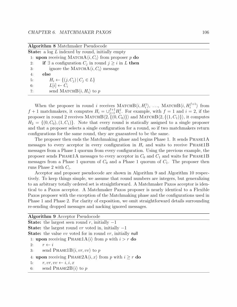
CHAPTER 6. MATCHMAKER PAXOS 106
Algorithm 8 Matchmaker Pseudocode
State: a log L indexed by round, initially empty1: upon receiving MatchA〈i, Ci〉 from proposer p do2: if ∃ a configuration Cj in round j ≥ i in L then3: ignore the MatchA〈i, Ci〉 message4: else5: Hi ← {(j, Cj) |Cj ∈ L}6: L[i]← Ci7: send MatchB〈i,Hi〉 to p
When the proposer in round i receives MatchB〈i,H1i 〉, . . ., MatchB〈i,Hf+1
i 〉 fromf + 1 matchmakers, it computes Hi = ∪f+1
j=1Hji . For example, with f = 1 and i = 2, if the
proposer in round 2 receives MatchB〈2, {(0, C0)}〉 and MatchB〈2, {(1, C1)}〉, it computesH2 = {(0, C0), (1, C1)}. Note that every round is statically assigned to a single proposerand that a proposer selects a single configuration for a round, so if two matchmakers returnconfigurations for the same round, they are guaranteed to be the same.
The proposer then ends the Matchmaking phase and begins Phase 1. It sends Phase1Amessages to every acceptor in every configuration in Hi and waits to receive Phase1Bmessages from a Phase 1 quorum from every configuration. Using the previous example, theproposer sends Phase1A messages to every acceptor in C0 and C1 and waits for Phase1Bmessages from a Phase 1 quorum of C0 and a Phase 1 quorum of C1. The proposer thenruns Phase 2 with Ci.
Acceptor and proposer pseudocode are shown in Algorithm 9 and Algorithm 10 respec-tively. To keep things simple, we assume that round numbers are integers, but generalizingto an arbitrary totally ordered set is straightforward. A Matchmaker Paxos acceptor is iden-tical to a Paxos acceptor. A Matchmaker Paxos proposer is nearly identical to a FlexiblePaxos proposer with the exception of the Matchmaking phase and the configurations used inPhase 1 and Phase 2. For clarity of exposition, we omit straightforward details surroundingre-sending dropped messages and nacking ignored messages.
Algorithm 9 Acceptor Pseudocode
State: the largest seen round r, initially −1State: the largest round vr voted in, initially −1State: the value vv voted for in round vr, initially null1: upon receiving Phase1A〈i〉 from p with i > r do2: r ← i3: send Phase1B〈i, vr, vv〉 to p
4: upon receiving Phase2A〈i, x〉 from p with i ≥ r do5: r, vr, vv ← i, i, x6: send Phase2B〈i〉 to p

CHAPTER 6. MATCHMAKER PAXOS 107
Algorithm 10 Proposer Pseudocode. Modifications to a Paxos proposer are underlined andshown in blue.State: a value x, initially nullState: a round i, initially −1State: the configuration Ci for round i, initially nullState: the prior configurations Hi for round i, initially null1: upon receiving value y from a client do2: i← next largest round owned by this proposer3: x← y4: Ci ← an arbitrary configuration5: send MatchA〈i, Ci〉 to all of the matchmakers
6: upon receiving MatchB〈i,H1i 〉, . . . ,MatchB〈i,Hf+1
i 〉 from f + 1 matchmakers do
7: Hi ←⋃f+1j=1 H
ji
8: send Phase1A〈i〉 to every acceptor in Hi
9: upon receiving Phase1B〈i,−,−〉 from a Phase 1 quorum from every configuration in10: Hi do11: k ← the largest vr in any Phase1B〈i, vr, vv〉12: if k 6= −1 then13: x← the corresponding vv in round k
14: send Phase2A〈i, x〉 to every acceptor in Ci
15: upon receiving Phase2B〈i〉 from a Phase 2 quorum do16: x is chosen, inform the client
Proof of Safety
We now prove that Matchmaker Paxos is safe; i.e. every execution of Matchmaker Paxoschooses at most one value.
Proof. Our proof is based on the Paxos safety proof in [41]. We prove, for every round i, thestatement P (i): “if a proposer proposes a value v in round i (i.e. sends a Phase2A messagefor value v in round i), then no value other than v has been or will be chosen in any roundless than i.” At most one value is ever proposed in a given round, so at most one value isever chosen in a given round. Thus, P (i) suffices to prove that Matchmaker Paxos is safefor the following reason. Assume for contradiction that Matchmaker Paxos chooses distinctvalues x and y in rounds j and i with j < i. Some proposer must have proposed y in roundi, so P (i) ensures us that no value other than y could have been chosen in round j. But, xwas chosen, a contradiction.
We prove P (i) by strong induction on i. P (0) is vacuous because there are no roundsless than 0. For the general case P (i), we assume P (0), . . . , P (i − 1). We perform a caseanalysis on the proposer’s pseudocode (Algorithm 10). Either k is −1 or it is not (line 11).

CHAPTER 6. MATCHMAKER PAXOS 108
First, assume it is not. In this case, the proposer proposes x, the value proposed in roundk (line 12). We perform a case analysis on round j to show that no value other than x hasbeen or will be chosen in any round j < i. That is, we show P (i).
Case 1: j > k. We show that no value has been or will be chosen in round j. Recallthat at the end of the Matchmaking phase, the proposer computed the set Hi of priorconfigurations using responses from a set Mi of f + 1 matchmakers. Either Hi contains aconfiguration Cj in round j or it doesn’t.
First, suppose it does. Then, the proposer sent Phase1A〈i〉 messages to all of theacceptors in Cj. A Phase 1 quorum of these acceptors, say Q, all received Phase1A〈i〉messages and replied with Phase1B messages. Thus, every acceptor in Q set its round r toi, and in doing so, promised to never vote in any round less than i. Moreover, none of theacceptors in Q had voted in any round greater than k. So, every acceptor in Q has not votedand never will vote in round j. For a value v′ to be chosen in round j, it must receive votesfrom some Phase 2 quorum Q′ of round j acceptors. But, Q and Q′ necessarily intersect, sothis is impossible. Thus, no value has been or will be chosen in round j.
Now suppose that Hi does not contain a configuration for round j. Hi is the union off + 1 MatchB messages from the f + 1 matchmakers in Mi. Thus, if Hi does not containa configuration for round j, then none of the MatchB messages did either. This meansthat for every matchmaker m ∈ Mi, when m received MatchA〈i, Ci〉, it did not contain aconfiguration for round j in its log. Moreover, by processing the MatchA〈i, Ci〉 request, thematchmaker is guaranteed to never process a MatchA〈j, Cj〉 request in the future. Thus,every matchmaker in Mi has not processed a MatchA request in round j and never will.For a value to be chosen in round j, the proposer executing round j must first receive repliesfrom f + 1 matchmakers, say Mj, in round j. But, Mi and Mj necessarily intersect, so thisis impossible. Thus, no value has been or will be chosen in round j.
Case 2: j = k. In a given round, at most one value is proposed, let alone chosen. x isthe value proposed in round k, so no other value could be chosen in round k.
Case 3: j < k. By induction, P (k) states that no value other than x has been or willbe chosen in any round less than k. This includes round j.
Finally, if k is −1, then we are in the same situation as in Case 1. No value has or willbe chosen in a round j < i.
Garbage Collection (How)
We’ve discussed how a proposer can change its round and introduce a new configuration.Now, we explain how to shut down old configurations. At the beginning of round i, a proposerp executes the Matchmaking phase and computes a set Hi of configurations in rounds lessthan i. The proposer then executes Phase 1 with the acceptors in these configurations.Assume Hi contains a configuration Cj for a round j < i. If we prematurely shut down theacceptors in Cj, then proposer p will get stuck in Phase 1, waiting for Phase1B messagesfrom a quorum of nodes that have been shut down. Therefore, we cannot shut down the

CHAPTER 6. MATCHMAKER PAXOS 109
acceptors in a configuration Cj until we are sure that the matchmakers will never againreturn Cj during the Matchmaking phase.
Thus, we extend Matchmaker Paxos to allow matchmakers to garbage collect configura-tions from their logs, ensuring that the garbage collected configurations will not be returnedduring any future Matchmaking phase. More concretely, a proposer p can now send aGarbageA〈i〉 command to the matchmakers informing them to garbage collect all config-urations in rounds less than i. When a matchmaker receives a GarbageA〈i〉 message, itdeletes log entry L[j] for every round j < i. It then updates a garbage collection watermarkw to the maximum of w and i and sends back a GarbageB〈i〉 message to the proposer.See Algorithm 11.
Algorithm 11 Matchmaker Pseudocode (with GC). Changes to Algorithm 8 are underlinedand shown in blue.State: a log L indexed by round, initially emptyState: a garbage collection watermark w, initially 01: upon receiving GarbageA〈i〉 from proposer p do2: delete L[j] for all j < i.3: w ← max(w, i)4: send GarbageB〈i〉 to p
5: upon receiving MatchA〈i, Ci〉 from proposer p do6: if i < w or ∃ Cj in round j ≥ i in L then7: ignore the MatchA〈i, Ci〉 message8: else9: Hi ← {(j, Cj) |Cj ∈ L}10: L[i]← Ci11: send MatchB〈i, w,Hi〉 to p
We also update the Matchmaking phase in three ways. First, a matchmaker ignores aMatchA〈i, Ci〉 message if i has been garbage collected (i.e. if i < w). Second, a matchmakerreturns its garbage collection watermark w in every MatchB that it sends. Third, when aproposer receives MatchB〈i, w1, H
1i 〉, . . ., MatchB〈i, wf+1, H
f+1i 〉 from f+1 matchmakers,
it again computes Hi = ∪f+1j=1H
ji . It then computes w = maxf+1
j=1 wj and prunes everyconfiguration in Hi in a round less than w. In other words, if any of the f + 1 matchmakershave garbage collected round j, then the proposer also garbage collects round j.
Once a proposer receives GarbageB〈i〉 messages from at least f +1 matchmakers M , itis guaranteed that all future Matchmaking phases will not include any configuration in anyround less than i. Why? Consider a future Matchmaking phase run with f +1 matchmakersM ′. M and M ′ intersect, so some matchmaker in the intersection has a garbage collectionwatermark at least as large as i. Thus, once a configuration has been garbage collected byf + 1 matchmakers, we can shut down the acceptors in the configuration.
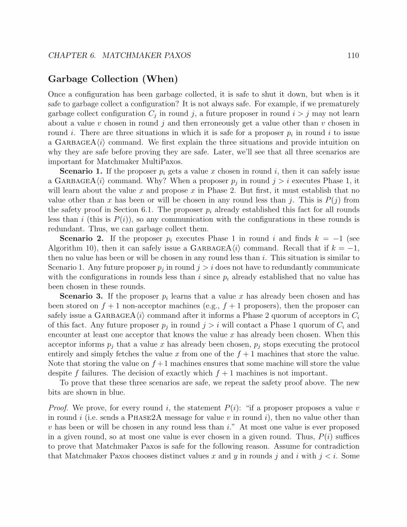
CHAPTER 6. MATCHMAKER PAXOS 110
Garbage Collection (When)
Once a configuration has been garbage collected, it is safe to shut it down, but when is itsafe to garbage collect a configuration? It is not always safe. For example, if we prematurelygarbage collect configuration Cj in round j, a future proposer in round i > j may not learnabout a value v chosen in round j and then erroneously get a value other than v chosen inround i. There are three situations in which it is safe for a proposer pi in round i to issuea GarbageA〈i〉 command. We first explain the three situations and provide intuition onwhy they are safe before proving they are safe. Later, we’ll see that all three scenarios areimportant for Matchmaker MultiPaxos.
Scenario 1. If the proposer pi gets a value x chosen in round i, then it can safely issuea GarbageA〈i〉 command. Why? When a proposer pj in round j > i executes Phase 1, itwill learn about the value x and propose x in Phase 2. But first, it must establish that novalue other than x has been or will be chosen in any round less than j. This is P (j) fromthe safety proof in Section 6.1. The proposer pi already established this fact for all roundsless than i (this is P (i)), so any communication with the configurations in these rounds isredundant. Thus, we can garbage collect them.
Scenario 2. If the proposer pi executes Phase 1 in round i and finds k = −1 (seeAlgorithm 10), then it can safely issue a GarbageA〈i〉 command. Recall that if k = −1,then no value has been or will be chosen in any round less than i. This situation is similar toScenario 1. Any future proposer pj in round j > i does not have to redundantly communicatewith the configurations in rounds less than i since pi already established that no value hasbeen chosen in these rounds.
Scenario 3. If the proposer pi learns that a value x has already been chosen and hasbeen stored on f + 1 non-acceptor machines (e.g., f + 1 proposers), then the proposer cansafely issue a GarbageA〈i〉 command after it informs a Phase 2 quorum of acceptors in Ciof this fact. Any future proposer pj in round j > i will contact a Phase 1 quorum of Ci andencounter at least one acceptor that knows the value x has already been chosen. When thisacceptor informs pj that a value x has already been chosen, pj stops executing the protocolentirely and simply fetches the value x from one of the f + 1 machines that store the value.Note that storing the value on f+1 machines ensures that some machine will store the valuedespite f failures. The decision of exactly which f + 1 machines is not important.
To prove that these three scenarios are safe, we repeat the safety proof above. The newbits are shown in blue.
Proof. We prove, for every round i, the statement P (i): “if a proposer proposes a value vin round i (i.e. sends a Phase2A message for value v in round i), then no value other thanv has been or will be chosen in any round less than i.” At most one value is ever proposedin a given round, so at most one value is ever chosen in a given round. Thus, P (i) sufficesto prove that Matchmaker Paxos is safe for the following reason. Assume for contradictionthat Matchmaker Paxos chooses distinct values x and y in rounds j and i with j < i. Some
CHAPTER 6. MATCHMAKER PAXOS 111
proposer must have proposed y in round i, so P (i) ensures us that no value other than ycould have been chosen in round j. But, x was chosen, a contradiction.
We prove P (i) by strong induction on i. P (0) is vacuous because there are no roundsless than 0. For the general case P (i), we assume P (0), . . . , P (i − 1). We perform a caseanalysis on the proposer’s pseudocode (Algorithm 10). Either k is −1 or it is not (line 11).First, assume it is not. In this case, the proposer proposes x, the value proposed in roundk (line 12). We perform a case analysis on round j to show that no value other than x hasbeen or will be chosen in any round j < i.
Case 1: j > k. We show that no value has been or will be chosen in round j. Recallthat at the end of the Matchmaking phase, the proposer computed the set Hi of priorconfigurations using responses from a set Mi of f + 1 matchmakers. Either Hi contains aconfiguration Cj in round j or it doesn’t.
First, suppose it does. Then, the proposer sent Phase1A〈i〉 messages to all of theacceptors in Cj. A Phase 1 quorum of these acceptors, say Q, all received Phase1A〈i〉messages and replied with Phase1B messages. Thus, every acceptor in Q set its round r toi, and in doing so, promised to never vote in any round less than i. Moreover, none of theacceptors in Q had voted in any round greater than k. So, every acceptor in Q has not votedand never will vote in round j. For a value v′ to be chosen in round j, it must receive votesfrom some Phase 2 quorum Q′ of round j acceptors. But, Q and Q′ necessarily intersect, sothis is impossible. Thus, no value has been or will be chosen in round j.
Now suppose that Hi does not contain a configuration for round j. Either a configurationCj was garbage collected from Hi or it wasn’t. First, assume it wasn’t. Then, Hi is theunion of f + 1 MatchB messages from the f + 1 matchmakers in Mi. Thus, if Hi does notcontain a configuration for round j, then none of the MatchB messages did either. Thismeans that for every matchmaker m ∈ Mi, when m received MatchA〈i, Ci〉, it did notcontain a configuration for round j in its log and never did. Moreover, by processing theMatchA〈i, Ci〉 request and inserting Ci in log entry i, the matchmaker is guaranteed tonever process a MatchA〈j, Cj〉 request in the future. Thus, every matchmaker in Mi hasnot processed a MatchA request in round j and never will. For a value to be chosen inround j, the proposer executing round j must first receive replies from f + 1 matchmakers,say Mj, in round j. But, Mi and Mj necessarily intersect, so this is impossible. Thus, novalue has been or will be chosen in round j.
Otherwise, a configuration Cj was garbage collected from Hi. Note that none of thematchmakers in Mi had received a GarbageA〈i′〉 command for a round i′ > i whenthey responded with their MatchB messages. If they had, they would have ignored ourMatchA〈i, Ci〉 message. Let i′ be the largest round j < i′ < i such that a matchmaker in Mi
had received a GarbageA〈i′〉 message before responding to our MatchA〈i, Ci〉 message.If i′ was garbage collected because of Scenario 1, then k would be at least as large as i′
since we would have intersected the Phase 2 quorum of Ci′ used in round i′ to get a valuechosen. But k < j < i′, a contradiction. If i′ was garbage collected because of Scenario 2,then we know no value has been or will be chosen in round j. If i′ was garbage collectedbecause of Scenario 3, then we would have intersected the Phase 2 quorum of Ci′ that knows

CHAPTER 6. MATCHMAKER PAXOS 112
a value was already chosen, and we would have not proposed a value in the first place. But,we proposed x, a contradiction.
Case 2: j = k. In a given round, at most one value is proposed, let alone chosen. x isthe value proposed in round k, so no other value could be chosen in round k.
Case 3: j < k. By induction, P (k) states that no value other than x has been or willbe chosen in any round less than k. This includes round j.
Finally, if k is −1, then we are in the same situation as in Case 1. No value has or willbe chosen in a round j < i.
Later, we’ll extend this garbage collection protocol to Matchmaker MultiPaxos (Sec-tion 6.2) and see empirically that matchmakers usually return just a single configuration(Section 6.5).
Optimizations
We now present a couple of protocol optimizations. First, note that a proposer can proac-tively run the Matchmaking phase in round i before it hears from a client. This is similarto proactively executing Phase 1, a standard optimization [29]. We call this optimizationproactive matchmaking.
Second, assume that the proposer in round i has executed the Matchmaking phase andPhase 1. Through Phase 1, it finds that k = −1 and thus learns that no value has beenchosen in any round less than i (see the safety proof above). Assume that before executingPhase 2 in round i, the proposer decides to perform a reconfiguration. To perform thereconfiguration, the proposer stops executing round i and begins executing the next roundi + 11. Typically to perform the reconfiguration, the proposer would have to execute theMatchmaking phase, Phase 1, and Phase 2 in round i + 1. However, in this case, afterexecuting the Matchmaking phase in round i+1, the proposer can skip Phase 1 and proceeddirectly to Phase 2. Why? The proposer established in round i that no value has been orwill be chosen in any round less than i. Moreover, because it did not run Phase 2 in roundi, it also knows that no value has been or will be chosen in round i. Together, these implythat no value has been or will be chosen in any round less than i+1. Normally, the proposerwould run Phase 1 in round i+1 to establish this fact, but since it has already established it,it can instead proceed directly to Phase 2. We call this optimization Phase 1 bypassing.
Phase 1 Bypassing depends on a proposer being the leader of round i and the leader ofthe next round i + 1. We can construct a set of rounds such that this is always the case.Let the set of rounds be the set of lexicographically ordered tuples (r, id, s) where r and sare both integers and id is a proposer id. A proposer is responsible for all the rounds thatcontain its id. With this set of rounds, the proposer p in round (r, p, s) always owns the nextround (r, p, s+ 1). For example given two proposers a and b, we have the following ordering
1Note that given a round i, we denote the next largest round in the total ordered set of rounds i + 1.We call this the “next round”.

CHAPTER 6. MATCHMAKER PAXOS 113
on rounds:
(0, a, 0) < (0, a, 1) < (0, a, 2) < (0, a, 3) < · · ·(0, b, 0) < (0, b, 1) < (0, b, 2) < (0, b, 3) < · · ·(1, a, 0) < (1, a, 1) < (1, a, 2) < (1, a, 3) < · · ·
We assume this round scheme throughout the rest of the chapter. In the next section, we’llsee that this optimization is essential for implementing Matchmaker MultiPaxos with goodperformance. Also note that this optimization is not particular to Matchmaker Paxos. Paxosand MultiPaxos can both take advantage of this optimization.
6.2 Matchmaker MultiPaxos
MultiPaxos
In Section 2.3, we discussed the normal case execution of Paxos. Now, we elaborate onMultiPaxos leader changes and the execution of Phase 1. Assume a proposer is electedleader in some round, say round i. We assume the leader knows that log entries up to andincluding log entry kc have already been chosen (e.g., by communicating with the replicas).We call this log entry the commit index. The leader then runs Phase 1 of Paxos in round ifor every log entry. Note that even though there are an infinite number of log entries largerthan kc, the leader can execute Phase 1 using a finite amount of information. In particular,the leader sends a single Phase1A〈i〉 message that acts as the Phase1A message for everylog entry larger than kc. Also, an acceptor replies with a Phase1B〈i, vr, vv〉 message onlyfor log entries in which the acceptor has voted. The infinitely many log entries in which theacceptor has not yet voted do not yield an explicit Phase1B message.
a
0
b
1
c
kc
d?
3 4
e?
kp 6 7 8
· · ·
Region 1:(already chosen)
Region 2:(maybe chosen)
Region 3:(not chosen)
Figure 6.3: A leader’s knowledge of the log after Phase 1.
The leader’s knowledge about the log after Phase 1 can be characterized by the commitindex kc and a pending index kp with kc ≤ kp, as shown in Figure 6.3. The commit indexand pending index divide the log into three regions: a prefix of chosen log entries (Region1), a suffix of unchosen log entries (Region 3), and a middle region of pending log entries(Region 2). More specifically:

CHAPTER 6. MATCHMAKER PAXOS 114
• Region 1 [0, kc]: The leader knows that a command has been chosen in every log entryless than or equal to kc.
• Region 3 [kp+1,∞): The leader knows that no command has been chosen (in any roundless than i) in any log entry larger than kp.
• Region 2 [kc + 1, kp]: If there is a command that may have already been chosen, thenit appears between kc and kp. Region 2 may also contain some log entries in which theleader knows (from executing a previous round) that a value has already been chosen, andit may contain some log entries in which the leader knows (from counting votes in Phase1) that no value has been chosen (we call these “holes”).
After Phase 1, the leader sends a Phase2A message for every unchosen log entry inRegion 2, proposing a “no-op” command for the holes. Simultaneously, the leader beginsaccepting client requests. When a client wants to propose a state machine command, itsends the command to the leader. The leader assigns log entries to commands in increasingorder, beginning at kp+ 1. It then runs Phase 2 of Paxos to get the command chosen in thatentry in round i. Once the leader learns that a command has been chosen in a given logentry, it informs the replicas. Replicas insert chosen commands into their logs and executethe logs in prefix order, sending the results of execution back to the clients.
It is critical to note that a leader performs Phase 1 of Paxos only once per round, notonce per command. In other words, Phase 1 is not performed during normal operation. Itis performed only when the leader fails and a new leader is elected in a larger round, anuncommon occurrence.
Matchmaker MultiPaxos
We first extend Matchmaker Paxos to Matchmaker MultiPaxos with proactive matchmakingbut without Phase 1 bypassing or garbage collection. We’ll see how to incorporate these twomomentarily. The extension from Matchmaker Paxos to Matchmaker MultiPaxos is analo-gous to the extension of Paxos to MultiPaxos. Matchmaker MultiPaxos reaches consensuson a totally ordered log of state machine commands, one log entry at a time, using oneinstance of Matchmaker Paxos for every log entry.
More concretely, a Matchmaker MultiPaxos deployment consists of an arbitrary numberof clients, at least f + 1 proposers, a set of 2f + 1 matchmakers, a dynamic set of acceptors(one configuration per round which can tolerate f failures), and a set of at least f + 1state machine replicas. We assume, as is standard, that a leader election algorithm is usedto select one of the proposers as a stable leader in some round, say round i. The leaderselects a configuration Ci of acceptors that it will use for every log entry. The mechanismby which the configuration is chosen is an orthogonal concern. A system administrator, forexample, could send the configuration to the leader, or the configuration could be read froman external service.

CHAPTER 6. MATCHMAKER PAXOS 115
The leader then executes the Matchmaking phase in the same way as in MatchmakerPaxos (i.e. it sends MatchA〈i, Ci〉messages to the matchmakers and awaits MatchB〈i,Hi〉responses). After the Matchmaking phase completes, the leader executes Phase 1 for everylog entry. This is identical to MultiPaxos, except that the leader uses the configurationsreturned by the matchmakers rather than assuming a fixed configuration. Note that proac-tive matchmaking allows the leader to execute the Matchmaking phase and Phase 1 beforereceiving any client requests.
The leader then enters Phase 2 and operates exactly as it would in MultiPaxos. Itexecutes Phase 2 with Ci for the log entries in Region 2. Moreover, when it receives a statemachine command from a client, it assigns the command a log entry in Region 3, runs Phase2 with the acceptors in Ci, and informs the replicas when the command is chosen. Replicasexecute commands in log order and send the results of executing commands back to theclients.
c1
c2
c3
p1
p2
m1 m2 m3
a1
a2
a3
b1b2
b3
1 122a
b
bc
c
d
(a) Matchmaking
c1
c2
c3
p1
p2
m1 m2 m3
a1
a2
a3
b1b2
b3
3
34
4
a
(b) Phase 1
c1
c2
c3
p1
p2
m1 m2 m3
a1
a2
a3
b1b2
b3
55
6 6
a
b
b
c
c
d
(c) Phase 2
Figure 6.4: An example Matchmaker MultiPaxos reconfiguration without Phase 1 bypassing.The leader p1 reconfigures from the acceptors a1, a2, a3 to the acceptors b1, b2, b3. Clientcommands are drawn as gray dashed lines. Note that every subfigure shows one phase of areconfiguration using solid colored lines, but the dashed lines show the complete execution ofa client request that runs concurrently with the reconfiguration. For simplicity, we assumethat every proposer also serves as a replica.
Discussion
To reconfigure from some old configuration Cold in round i to some new configuration Cnew,the Matchmaker MultiPaxos leader of round i simply advances to round i+1 and selects thenew configuration Cnew. The new configuration is active immediately after the Matchmakingphase, a one round trip delay. Note that the acceptors in the new configuration Cnew do nothave to undergo any sort of warm up or bootstrapping and do not have to contact any otheracceptors in any other configuration.

CHAPTER 6. MATCHMAKER PAXOS 116
The new configuration is active immediately, but it is not safe to deactivate the acceptorsin the old configuration immediately, as we saw in Section 6.1. We extend MatchmakerPaxos’s garbage collection to Matchmaker MultiPaxos momentarily.
Also note that Matchmaker MultiPaxos does not perform the Matchmaking phase orPhase 1 on the critical path of normal execution. Similar to how MultiPaxos executes Phase1 only once per leader change (and not once per command), Matchmaker MultiPaxos runsthe Matchmaking phase and Phase 1 only when a new leader is elected or when a leaderchanges its round (e.g., when a leader transitions from round i to round i + 1 as part ofa reconfiguration). In the normal case (i.e. during Phase 2), Matchmaker MultiPaxos andMultiPaxos are identical, and Matchmaker MultiPaxos does not introduce any overheads. Inthe normal case, Matchmaker MultiPaxos deploys a single stable leader that changes roundsonly to perform a reconfiguration. Changing from one leader to another only happens aftera leader has failed.
Furthermore, configurations do not have to be unique across rounds. The leader in roundi is free to re-use a configuration Cj that was used in some round j < i.
Optimization
Ideally, Matchmaker MultiPaxos’ performance would be unaffected by a reconfiguration. Thelatency of every client request and the protocol’s overall throughput would remain constantthroughout a reconfiguration. Matchmaker MultiPaxos as we’ve described it so far, however,does not meet this ideal. During a reconfiguration, a leader must temporarily stop processingclient commands and wait for the reconfiguration to finish before resuming normal operation.
This is illustrated in Figure 6.4. Figure 6.4 shows a leader p1 reconfiguring from aconfiguration of acceptors Cold consisting of acceptors a1, a2, and a3 in round i to a newconfiguration of acceptors Cnew consisting of acceptors b1, b2, and b3 in round i + 1. Whilethe leader performs the reconfiguration, clients continue to send state machine commands tothe leader. We consider such a command and perform a case analysis on when the commandarrives at the leader to see whether or not the command has to be stalled.
Case 1: Matchmaking (Figure 6.4a). If the leader receives a command during theMatchmaking phase, then the leader can process the command as normal in round i usingthe acceptors in Cold. Even though the leader is executing the Matchmaking phase in roundi+ 1 and is communicating with the matchmakers, the acceptors in Cold are oblivious to thisand can process commands in Phase 2 in round i.
Case 2: Phase 1 (Figure 6.4b). If the leader receives a command during Phase 1,then the leader cannot process the command. It must delay the processing of the commanduntil Phase 1 finishes. Here’s why. Once an acceptor in Cold receives a Phase1A〈i + 1〉message, it will reject any future commands in rounds less than i+ 1, so the leader is unableto send the command to Cold. The leader also cannot send the command to Cnew in roundi+ 1 because it has not yet finished executing Phase 1.
Case 3: Phase 2 (Figure 6.4c). If the leader receives a command during Phase 2,then the leader can send the command to the new acceptors in Cnew in round i+ 1. This is

CHAPTER 6. MATCHMAKER PAXOS 117
the normal case of execution.In summary, any commands received during Phase 1 of a reconfiguration are delayed.
Fortunately, we can eliminate this problem by using Phase 1 bypassing. Consider a leaderperforming a reconfiguration from Ci in round i to Ci+1 in round i + 1. At the end of theMatchmaking phase and at the beginning of Phase 1 (in round i+1), let k be the largest logentry that the leader has assigned to a command. That is, all log entries after entry k areempty. These log entries satisfy the preconditions of Phase 1 bypassing, so it is safe for theleader to bypass Phase 1 in round i + 1 for these log entries in the following way. When aleader receives a command after the Matchmaking phase, it assigns the command a log entrylarger than k, skips Phase 1, and executes Phase 2 in round i+ 1 with Cnew immediately.
With this optimization and the round scheme described in Section 6.1, no state machinecommands are delayed. Commands received during the Matchmaking phase or earlier arechosen in round i by Cold in log entries up to and including k. Commands received duringPhase 1, Phase 2, or later are chosen in round i + 1 by Cnew in log entries k + 1, k + 2,k + 3, and so on. With this optimization Matchmaker MultiPaxos can be reconfigured withminimal performance degradation.
Garbage Collection
Recall that the Matchmaker MultiPaxos leader pi in round i uses a single configuration Ci forevery log entry. The leader pi can safely issue a GarbageA〈i〉 command to the matchmakersonce it ensures that every log entry satisfies one of the three scenarios described in Section 6.1.Recall from Figure 6.3 that at the end of Phase 1 and at the beginning of Phase 2, the logcan be divided into three regions. Each of the three garbage collection scenarios applies toone of the regions.
Scenario 2 applies to Region 3. These are the log entries for which k = −1. Scenario1 applies to Region 2, once the leader has successfully chosen commands in all of the logentries in Region 2. Scenario 3 applies to Region 1 if we make the following adjustments.First, we deploy 2f + 1 replicas instead of f + 1. Second, the leader ensures that the prefixof previously chosen log entries is stored on at least f + 1 of the 2f + 1 replicas. Third,the leader informs a Phase 2 quorum of Ci acceptors that these commands have been storedon the replicas. Every replica maintains a copy of the log of state machine commands andcannot discard a command after execution. The log must also be garbage collected over time,for example, by using snapshots [67]. Note that garbage collecting the log is an orthogonal(but also complicated) issue from garbage collecting old configurations. It must be doneregardless of reconfigurations and is outside of the scope of this thesis.
In summary, the leader pi of round i executes as follows. It executes the Matchmakingphase to get the prior configurations Hi. It executes Phase 1 with the configurations in Hi.It enters Phase 2 and chooses commands in Region 2. It informs a Phase 2 quorum of Ciacceptors once the commands in Region 1 have been stored on f + 1 replicas. It issues aGarbageA〈i〉 command to the matchmakers and awaits f + 1 GarbageB〈i〉 responses.At this point, all previous configurations can be shut down.

CHAPTER 6. MATCHMAKER PAXOS 118
Note that the leader can begin processing state machine commands from clients as soonas it enters Phase 2. It does not have to stall commands during garbage collection. Notealso that during normal operation, old configurations are garbage collected very quickly. InSection 6.5, we show that Hi almost always contains a single configuration (i.e. Ci−1).
6.3 Reconfiguring Matchmakers
We’ve discussed how Matchmaker MultiPaxos allows us to reconfigure the set of acceptors.In this section, we discuss how to reconfigure proposers, replicas, and matchmakers (them-selves).
Reconfiguring proposers and replicas is straightforward. In fact, Matchmaker MultiPaxosreconfigures proposers and replicas in exactly the same way as MultiPaxos [87], so we donot discuss it at length. In short, a proposer can be safely added or removed at any time.Replicas can also be safely added or removed at any time so long as we ensure that commandsreplicated on f + 1 replicas remain replicated on f + 1 replicas. This is a difficult, yetorthogonal challenge. Existing approaches can be adopted by Matchmaker MultiPaxos [68].For performance, a newly introduced proposer should contact an existing proposer or replicato learn about the prefix of already chosen commands, and a newly introduced replica shouldcopy the log from an existing replica.
Reconfiguring matchmakers is a bit more involved, but still relatively straightforward.Recall that proposers perform the Matchmaking phase only during a change in round. Thus,for the vast majority of the time—specifically, when there is a single, stable leader—thematchmakers are completely idle. This means that the way we reconfigure the matchmakershas to be safe, but it doesn’t have to be efficient. The matchmakers can be reconfigured atany time between round changes without any impact on the performance.
Thus, we use the simplest approach to reconfiguration: we shut down the old matchmak-ers and replace them with new ones, making sure that the new matchmakers’ initial state isthe same as the old matchmakers’ final state. More concretely, we reconfigure from a set Mold
of matchmakers to a new set Mnew as follows. First, a proposer (or any other node) sends aStopA〈〉 message to the matchmakers in Mold. When a matchmaker mi receives a StopA〈〉message, it stops processing messages (except for other StopA〈〉 messages) and replies withStopB〈Li, wi〉 where Li is mi’s log and wi is its garbage collection watermark. When theproposer receives StopB messages from f + 1 matchmakers, it knows that the matchmakershave effectively been shut down. It computes w as the maximum of every returned wi. Itcomputes L as the union of the returned logs, and removes all entries of L that appear in around less than w. An example of this log merging is illustrated in Figure 6.5.
The proposer then sends L and w to all of the matchmakers in Mnew. Each matchmakeradopts these values as its initial state. At this point, the matchmakers in Mnew cannot beginprocessing commands yet. Naively, it is possible that two different nodes could simultane-ously attempt to reconfigure to two disjoint sets of matchmakers, say Mnew and M ′
new.

CHAPTER 6. MATCHMAKER PAXOS 119
C0(w) 0
C11
2
3
C44
L0
×0
×1
C2(w) 2
3
4
L1
×0
C1(w) 1
C22
3
4
L2
×0
×1
C2(w) 2
3
C44
Figure 6.5: An example of merging three matchmaker logs (L0, L1, and L2) during a match-maker reconfiguration. Garbage collected log entries are shown in red.
To avoid this, every matchmaker in Mold doubles as a Paxos acceptor. A proposerattempting to reconfigure to Mnew acts as a Paxos proposer and gets the value Mnew chosenby the matchmakers (which are acting as Paxos acceptors). Once Mnew is chosen, theproposer notifies the matchmakers in Mnew that the reconfiguration is complete and thatthey are free to start processing commands.
If a proposer contacts a stale set of matchmakers (e.g., Mold), the matchmakers informthe proposer of their successors (e.g., Mnew). This newer set of matchmakers may also bestale, so the proposer repeatedly polls stale matchmakers until it finds the active set ofmatchmakers. In this way, the matchmakers form a chain, with each set of matchmakerspointing to its successor.
Before a set of matchmakers can be shut down, the identity of its successors must bepersisted in some name service (e.g., DNS). Ideally for performance, the name service wouldalways point to the active set of matchmakers, but this is not required for safety.
We now prove that Matchmaker MultiPaxos is still safe, even with matchmaker recon-figurations. The new bits are shown in blue.
Proof. We prove, for every round i, the statement P (i): “if a proposer proposes a value vin round i (i.e. sends a Phase2A message for value v in round i), then no value other thanv has been or will be chosen in any round less than i.” At most one value is ever proposedin a given round, so at most one value is ever chosen in a given round. Thus, P (i) sufficesto prove that Matchmaker Paxos is safe for the following reason. Assume for contradictionthat Matchmaker Paxos chooses distinct values x and y in rounds j and i with j < i. Someproposer must have proposed y in round i, so P (i) ensures us that no value other than ycould have been chosen in round j. But, x was chosen, a contradiction.
We prove P (i) by strong induction on i. P (0) is vacuous because there are no roundsless than 0. For the general case P (i), we assume P (0), . . . , P (i − 1). We perform a caseanalysis on the proposer’s pseudocode (Algorithm 10). Either k is −1 or it is not (line 11).

CHAPTER 6. MATCHMAKER PAXOS 120
First, assume it is not. In this case, the proposer proposes x, the value proposed in roundk (line 12). We perform a case analysis on round j to show that no value other than x hasbeen or will be chosen in any round j < i.
Case 1: j > k. We show that no value has been or will be chosen in round j. Recallthat at the end of the Matchmaking phase, the proposer computed the set Hi of priorconfigurations using responses from a set Mi of f + 1 matchmakers. Either Hi contains aconfiguration Cj in round j or it doesn’t.
First, suppose it does. Then, the proposer sent Phase1A〈i〉 messages to all of theacceptors in Cj. A Phase 1 quorum of these acceptors, say Q, all received Phase1A〈i〉messages and replied with Phase1B messages. Thus, every acceptor in Q set its round r toi, and in doing so, promised to never vote in any round less than i. Moreover, none of theacceptors in Q had voted in any round greater than k. So, every acceptor in Q has not votedand never will vote in round j. For a value v′ to be chosen in round j, it must receive votesfrom some Phase 2 quorum Q′ of round j acceptors. But, Q and Q′ necessarily intersect, sothis is impossible. Thus, no value has been or will be chosen in round j.
Now suppose that Hi does not contain a configuration for round j. Either a configurationCj was garbage collected from Hi or it wasn’t. First, assume it wasn’t. Then, Hi is theunion of f + 1 MatchB messages from the f + 1 matchmakers in Mi. Thus, if Hi doesnot contain a configuration for round j, then none of the MatchB messages did either.This means that for every matchmaker m ∈ Mi, when m received MatchA〈i, Ci〉, it didnot contain a configuration for round j in its log and never did. Moreover, no majority inany previous set of matchmakers contained a configuration in round j. If any majority didhave a configuration in round j, then all subsequent matchmakers would as well since a setof matchmakers is initialized from a majority of the previous matchmakers. Moreover, byprocessing the MatchA〈i, Ci〉 request and inserting Ci in log entry i, the matchmaker isguaranteed to never process a MatchA〈j, Cj〉 request in the future. Moreover, no futureset of matchmakers will either. A majority of matchmakers have a configuration in entry i,so all subsequent configurations will as well. Therefore, they will all reject a configurationin round j. Thus, every matchmaker in Mi has not processed a MatchA request in roundj and never will. For a value to be chosen in round j, the proposer executing round j mustfirst receive replies from f+1 matchmakers, say Mj, in round j. But, Mi and Mj necessarilyintersect, so this is impossible. This argument holds for every set of matchmakers. Thus, novalue has been or will be chosen in round j.
Otherwise, a configuration Cj was garbage collected from Hi. Note that none of thematchmakers in Mi had received a GarbageA〈i′〉 command for a round i′ > i whenthey responded with their MatchB messages. If they had, they would have ignored ourMatchA〈i, Ci〉 message. Similarly, none of the matchmakers in Mi were initialized with agarbage collection watermark w > i. Let i′ be the largest round j < i′ < i that a matchmakerin Mi garbage collected before responding to our MatchA〈i, Ci〉 message.
If i′ was garbage collected because of Scenario 1, then k would be at least as large as i′
since we would have intersected the Phase 2 quorum of Ci′ used in round i′ to get a valuechosen. But k < j < i′, a contradiction. If i′ was garbage collected because of Scenario 2,

CHAPTER 6. MATCHMAKER PAXOS 121
then we know no value has been or will be chosen in round j. If i′ was garbage collectedbecause of Scenario 3, then we would have intersected the Phase 2 quorum of Ci′ that knowsa value was already chosen, and we would have not proposed a value in the first place. But,we proposed x, a contradiction.
Case 2: j = k. In a given round, at most one value is proposed, let alone chosen. x isthe value proposed in round k, so no other value could be chosen in round k.
Case 3: j < k. We can apply the inductive hypothesis to get P (k) which states that novalue other than x has been or will be chosen in any round less than k. This includes roundj, which is exactly what we’re trying to prove.
Finally, if k is −1, then we are in the same situation as in Case 1.
6.4 Theoretical Insights
MultiPaxos To reconfigure from a set of nodes N to a new set of nodes N ′, a MultiPaxosleader gets the value N ′ chosen in the log at some index i. All commands in the log startingat position i+α are chosen using the nodes in N ′ instead of the nodes in N , where α is someconfigurable parameter. This protocol is called Horizontal MultiPaxos.
a
0
b
1
c
2
N ′
3
d
4
no-op
5
no-op
6
e
7
f
8
· · ·
α
chosen with N chosen with N ′
Figure 6.6: A MultiPaxos log during reconfiguration (α = 4).
Matchmaker MultiPaxos has the following advantages over Horizontal MultiPaxos. First,the core idea behind Horizontal MultiPaxos seems simple, but the protocol has a numberof hidden subtleties [54]. For example, a newly elected Horizontal MultiPaxos leader witha stale log may not know the latest configuration of nodes. It may not even know whichconfiguration of nodes to contact to learn the latest configuration of nodes. This makes itunclear when it is safe to shut down old configurations because a newly elected HorizontalMultiPaxos leader can be arbitrarily out of date. These subtleties and the many othersdescribed in [54] makes Horizontal MultiPaxos significantly more complicated that it initiallyseems. Matchmaker Paxos addresses these subtleties directly. The matchmakers can alwaysbe used to learn the latest configuration, and our garbage collection protocol details exactlywhen and how to shut down old configurations safely.
Second, horizontal reconfiguration is not generally applicable. It is fundamentally in-compatible with replication protocols that do not replicate a log. Moreover, researchers arefinding that avoiding a log can often be advantageous [42, 62, 6, 74, 97, 82, 21]. For example,

CHAPTER 6. MATCHMAKER PAXOS 122
protocols like Generalized Paxos [42], EPaxos [62], Atlas [21], and Caesar [6] arrange com-mands in a partially ordered graph instead of a totally ordered log to exploit commutativitybetween commands. CASPaxos [74] maintains a single value, instead of a log or graph,for simplicity. Databases like TAPIR [97] avoid ordering transactions in a log for improvedperformance, and databases like Meerkat [82] do the same to improve scalability. Even someprotocols with logs cannot use the ideas behind Horizontal MultiPaxos. For example, Raftcannot safely perform Horizontal MultiPaxos’ reconfiguration [67].
Because these protocols do not replicate logs, they cannot use MultiPaxos’ horizontalreconfiguration protocol. However, while none of the protocols replicate logs, all of themhave rounds. This means that the protocols can either use Matchmaker Paxos directly, orat least borrow ideas from Matchmaker Paxos for reconfiguration. For example, we aredeveloping a protocol called BPaxos that is an EPaxos [62] variant which partially orderscommands into a graph. BPaxos is a modular protocol that uses Paxos as a black boxsubroutine. Due to this modularity, we can directly replace Paxos with Matchmaker Paxosto support reconfiguration. The same idea can also be applied to EPaxos. CASPaxos [74]is similar to Paxos and can be extended to Matchmaker CASPaxos in the same way weextended Paxos to Matchmaker Paxos. These are two simple examples, and we don’t claimthat extending Matchmaker Paxos to some of the other more complicated protocols is alwayseasy. But, the universality of rounds makes Matchmaker Paxos an attractive foundation ontop of which other non-log based protocols can build their own reconfiguration protocols.
One could argue that these other protocols are not used as much in industry, so it’s notthat important for them to have reconfiguration protocols, but we think the causation is inthe reverse direction! Without reconfiguration, these protocols cannot be used in industry.
Third, optimizing Horizontal MultiPaxos is not easy. A MultiPaxos leader can processat most α unchosen commands at a time. This makes α an important parameter to tune.If we set α too low, then we limit the protocol’s pipeline parallelism and the throughputsuffers. Note that a small α reduces the normal case throughput of Horizontal MultiPaxos,not just the throughput during reconfiguration. If we set α too high, then we have towait a long time for a reconfiguration to complete. If we are reconfiguring because of afailed node, then we might have to endure a long reconfiguration with reduced throughput.Matchmaker MultiPaxos has no α parameter to tune. Note that Horizontal MultiPaxoscan be implemented with an optimization in which we select a very large α and then geta sequence of α noops in the log to force a quick reconfiguration. This optimization helpsavoid the difficulties of finding a good value of α, but the optimization introduces a newset of subtleties into the protocol. For example, the leader cannot process client requestswhile it is executing Phase 2 for the α noops. The protocol has to implement additionalmechanisms to avoid this one round trip stall.
Foruth, Horizontal MultiPaxos requires a Phase 1 and Phase 2 quorum of acceptorsfrom an old configuration in order to perform a reconfiguration after a leader failure, butMatchmaker MultiPaxos only requires a Phase 1 quorum. Some read optimized MultiPaxosvariants perform reads against Phase 1 quorums [13]. These protocols benefit from havingvery small Phase 1 quorums and very large Phase 2 quorums, requiring Horizontal Multi-

CHAPTER 6. MATCHMAKER PAXOS 123
Paxos to contact far more nodes that Matchmaker MultiPaxos during a reconfiguration.Finally, we clarify that if Horizontal MultiPaxos is implemented with all of its subtleties
ironed out, is deployed with a good choice of α, and is run with small Phase 2 quorums, thenit can perform a reconfiguration without performance degradation. In this case, HorizontalMultiPaxos and Matchmaker MultiPaxos both reconfigure, in some sense, “optimally”.
Vertical Paxos Matchmaker MultiPaxos significantly improves the practicality of Verti-cal Paxos [49] in a number of ways. First, Vertical Paxos is a consensus protocol, not astate machine replication protocol, and it’s not easy to extend Vertical Paxos’ garbage col-lection protocol to a state machine replication protocol. Vertical Paxos garbage collects oldconfigurations in situations similar to Scenario 1 and Scenario 2 from Section 6.1. It doesnot include Scenario 3. Without this, old configurations cannot be garbage collected, whichmeans that it is never safe to shut down old configurations.
Second, Vertical Paxos requires an external master but does not describe how to imple-ment the master in an efficient way. We could implement the master using another statemachine replication protocol like MultiPaxos, but this would be both slow and overly com-plex. Plus, we would have to implement a reconfiguration protocol for the master as well.Our matchmakers are analogous to the external master but show that such a master doesnot require a nested invocation of state machine replication.
Third, Vertical Paxos requires that a proposer execute Phase 1 in order to perform areconfiguration. Thus, Vertical Paxos cannot be extended to MultiPaxos without causingperformance degradation during reconfiguration. This is not the case for matchmakers thanksto Phase 1 bypassing.
Fourth, Vertical Paxos does not describe how proposers learn the configurations used inprevious rounds and instead assumes that configurations are fixed in advance by an oracle.Matchmaker Paxos shows that this assumption is not necessary, as the matchmakers storeevery configuration.
Fast Paxos While Paxos quorums consist of f + 1 out of 2f + 1 acceptors, Fast Paxosrequires larger quorums. Many protocols have reduced Fast Paxos quorum sizes a bit, but todate, Fast Paxos quorum sizes have remained larger than classic Paxos quorum sizes [62, 21].Using matchmakers, we can implement Fast Paxos with a fixed set of f + 1 acceptors (andhence with f + 1-sized quorums). Specifically, we deploy Fast Paxos with f + 1 acceptors,with a single unanimous Phase 2 quorum, and with singleton Phase 1 quorums.
Fast Paxos proposer pseudocode is given in Algorithm 12. We do not modify the FastPaxos acceptor or the matchmakers. For simplicity, we assume that we deploy Fast Paxoswith f + 1 acceptors, with a single unanimous Phase 2 quorum, and with singleton Phase1 quorums. Generalizing to arbitrary configurations that satisfy Fast Paxos’ quorum in-tersection requirements is straightforward. Note that Fast Paxos cannot leverage Phase 1Bypassing. Also note while both MultiPaxos and our Fast Paxos variant both have quorumsof size f + 1, our Fast Paxos variant has a fixed set of f + 1 acceptors, while MultiPaxos can

CHAPTER 6. MATCHMAKER PAXOS 124
Algorithm 12 Fast Paxos Proposer Pseudocode
State: a round i, initially −1State: the configuration Ci for round i, initially nullState: the prior configurations Hi for round i, initially null1: i← next largest round owned by this proposer2: Ci ← an arbitrary configuration3: send MatchA〈i, Ci〉 to all of the matchmakers4: upon receiving MatchB〈i,H1
i 〉, . . . ,MatchB〈i,Hf+1i 〉 from f + 1 matchmakers do
5: Hi ←⋃f+1j=1 H
ji
6: send Phase1A〈i〉 to every acceptor in Hi
7: upon receiving Phase1B〈i,−,−〉 from a Phase 1 quorum from every configuration inHi do
8: k ← the largest vr in any Phase1B〈i, vr, vv〉9: V ← the corresponding vv’s in round k10: if k = −1 then11: send Phase2A〈i, any〉 to every acceptor in Ci12: else if V = {v} then13: send Phase2A〈i, v〉 to every acceptor in Ci14: else15: send Phase2A〈i, any〉 to every acceptor in Ci
choose any set of f + 1 acceptors from all 2f + 1 acceptors. This has some disadvantages interms of tail latency and fault tolerance.
We now prove that our modifications to Fast Paxos are safe. For simplicity, we ignoregarbage collection and matchmaker reconfiguration. Introducing those two features andproving them correct is pretty much identical to what we did with Matchmaker Paxos.
Proof. We prove, for every round i, the statement P (i) which states that if a an acceptorvotes for a value v in round i (i.e. sends a Phase2B message for value v in round i), then novalue other than v has been or will be chosen in any round less than i. P (i) suffices to provethat Matchmaker Paxos is safe. Why? Well, assume for contradiction that MatchmakerPaxos chooses distinct values x and y in rounds i and j with i < j. Some acceptor musthave voted for y in round j, so P (j) ensures us that no value other than y could have beenchosen in round i. But, x was chosen, a contradiction.
We prove P (i) by strong induction on i. P (0) is vacuous because there are no roundsless than 0. For the general case P (i), we assume P (0), . . . , P (i − 1). We perform a caseanalysis on the proposer’s pseudocode. Either k is −1 or it is not (line 8). First, assume itis not. We perform a case analysis on rounds j < i.
Case 1: j > k. Recall that at the end of the Matchmaking phase, the proposer computedthe set Hi of prior configurations using responses from a set M of f+1 matchmakers. EitherHi contains a configuration Cj in round j or it doesn’t.

CHAPTER 6. MATCHMAKER PAXOS 125
First, suppose it does. Then, the proposer sent Phase1A〈i〉 messages to all of theacceptors in Cj. A Phase 1 quorum of these acceptors, say Q, all received Phase1A〈i〉messages and replied with Phase1B messages. Thus, every acceptor in Q set its round r toi, and in doing so, promised to never vote in any round less than i. Moreover, none of theacceptors in Q had voted in any round greater than k. So, every acceptor in Q has not votedand never will vote in round j. For a value v′ to be chosen in round j, it must receive votesfrom some Phase 2 quorum Q′ of round j acceptors. But, Q and Q′ necessarily intersect, sothis is impossible. Thus, no value has been or will be chosen in round j.
Now suppose that Hi does not contain a configuration for round j. Hi is the union off + 1 MatchB messages from the f + 1 matchmakers in M . Thus, if Hi does not containa configuration for round j, then none of the MatchB messages did either. This meansthat for every matchmaker m ∈ M , when m received MatchA〈i, Ci〉, it did not contain aconfiguration for round j in its log. Moreover, by processing the MatchA〈i, Ci〉 request andinserting Ci in log entry i, the matchmaker is guaranteed to never process a MatchA〈j, Cj〉request in the future. Thus, every matchmaker in M has not processed a MatchA requestin round j and never will. For a value to be chosen in round j, the proposer executing roundj must first receive replies from f + 1 matchmakers, say M ′, in round j. But, M and M ′
necessarily intersect, so this is impossible. Thus, no value has been or will be chosen inround j.
Case 2: j = k. If V = {v}, then the proposer proposes v. We must prove that no valueother than v has been or will be chosen in round k. For a value to be chosen in round k,every acceptor must vote for it in round k. Some acceptor voted for v in round k, so it isthe only value with the possibility of receiving a unanimous vote.
Otherwise V contains multiple distinct elements, and the proposer proposes any. Wemust prove that no value has been or will be chosen in round k. This is immediate since novalue can receive a unanimous vote in round k, if two different values have received votes inround k.
Case 3: j < k. If V = {v}, then the proposer proposes v, and we must prove that novalue other than v has been or will be chosen in any round less than k. This is immediatefrom P (k). Otherwise, V = {v1, v2, . . .}, and the proposer proposes any. We must prove thatno value has been or will be chosen in any round less than k. P (k) tells us that no valueother than v1 has been or will be chosen in any round less than k. P (k) also tells us that novalue other than v2 has been or will be chosen in any round less than k. Thus, no value hasbeen or will be chosen in any round less than k.
Finally, if k is −1, then we are in the same situation as in Case 1. No value has been orwill be chosen in any round less than i.
DPaxos DPaxos is a Paxos variant that allows every round to use a different subset ofacceptors from some fixed set of acceptors. Matchmaker Paxos obviates the need for afixed set of nodes. DPaxos’ scope is limited to a single instance of consensus, whereasMatchmaker MultiPaxos shows how to efficiently reconfigure across multiple instances of

CHAPTER 6. MATCHMAKER PAXOS 126
consensus simultaneously. We also discovered that DPaxos’ garbage collection algorithm isunsafe. Matchmaker MultiPaxos fixes the bug.
Consider a DPaxos deployment with fd = 1, fz = 0, three zones, three nodes per zone,and delegate quorums. Thus, a replication quorum consists of two nodes in one zone, and aleader election quorum consists of two nodes in two zones. We name the nodes A throughI. Beside each node, we display its ballot, vote ballot, vote value, and intents [44].
Zone 1
A
B
C
Zone 2
D
E
F
Zone 3
G
H
I
−1,−1,⊥, ∅
−1,−1,⊥, ∅
−1,−1,⊥, ∅
−1,−1,⊥, ∅
−1,−1,⊥, ∅
−1,−1,⊥, ∅
−1,−1,⊥, ∅
−1,−1,⊥, ∅
−1,−1,⊥, ∅
Proposer 1 initiates the leader election phase in ballot 0 for value x. It selects {A,B,D,E}as its leader election quorum and {B,C} as its intent. It sends prepare messages to theleader election quorum, and the leader election quorum replies. Proposer 1 doesn’t receiveany intents, so it does not expand its leader election quorum. It also learns that no valuehas been chosen yet, so it proposes value x to B and C. Both accept the value.
Zone 1
A
B
C
Zone 2
D
E
F
Zone 3
G
H
I
0,−1,⊥, {0 : {B,C}}
0, 0, x, {0 : {B,C}}
0, 0, x, ∅
0,−1,⊥, {0 : {B,C}}
0,−1,⊥, {0 : {B,C}}
−1,−1,⊥, ∅
−1,−1,⊥, ∅
−1,−1,⊥, ∅
−1,−1,⊥, ∅
Next, proposer 2 initiates the leader election phase in ballot 1 for value y. It selects{E,F,H, I} as its leader election quorum and {G,H} as its intent. It sends prepare messagesto the leader election quorum, and the leader election quorum replies. Proposer 2 receivesthe intent {B,C} in ballot 0 from E, so it expands its leader election quorum and sends aprepare message to C. Proposer 2 learns that value x was chosen in ballot 0, so it ditches yand proposes x to G and H. G accepts, but the propose message to H is dropped.

CHAPTER 6. MATCHMAKER PAXOS 127
Zone 1
A
B
C
Zone 2
D
E
F
Zone 3
G
H
I
0,−1,⊥, {0 : {B,C}}
0, 0, x, {0 : {B,C}}
0, 0, x, {1 : {G,H}}
0,−1,⊥, {0 : {B,C}}
1,−1,⊥, {0 : {B,C}, 1 : {G,H}}
1,−1,⊥, {1 : {G,H}}
1, 1, x, ∅
1,−1,⊥, {1 : {G,H}}
1,−1,⊥, {1 : {G,H}}
Next, garbage collection is run. The garbage collector contacts G and sees that it hasaccepted a value in ballot 1. It informs all the nodes to discard intents in ballots less than 1.
Zone 1
A
B
C
Zone 2
D
E
F
Zone 3
G
H
I
0,−1,⊥, ∅
0, 0, x, ∅
0, 0, x, {1 : {G,H}}
0,−1,⊥, ∅
1,−1,⊥, {1 : {G,H}}
1,−1,⊥, {1 : {G,H}}
1, 1, x, ∅
1,−1,⊥, {1 : {G,H}}
1,−1,⊥, {1 : {G,H}}
Next, proposer 3 initiates the leader election phase in ballot 2 for value z It selects{D,E,H, I} as its leader election quorum and {E,F} as its intent. It sends prepare messagesto the leader election quorum, and the leader election quorum replies. Proposer 3 receivesintent {G,H} in ballot 1, but has already included H in its leader election quorum, so itdoes not send any additional prepares. It learns that no value has been chosen (this is a bug,x was chosen), so it proposes value z to E and G. Both accept the value, and z is chosen.This is a bug since x was already chosen.
Zone 1
A
B
C
Zone 2
D
E
F
Zone 3
G
H
I
0,−1,⊥, ∅
0, 0, x, ∅
0, 0, x, {1 : {G,H}}
2,−1,⊥, ∅2 : {E,F}
2, 2, z, {1 : {G,H}, 2 : {E,F}}
2, 2, z, {1 : {G,H}}
1, 1, x, ∅
2,−1,⊥, {1 : {G,H}, 2 : {E,F}}
2,−1,⊥, {1 : {G,H}, 2 : {E,F}}

CHAPTER 6. MATCHMAKER PAXOS 128
6.5 Evaluation
We now evaluate Matchmaker MultiPaxos. Matchmaker MultiPaxos is implemented in Scalausing the Netty networking library. We deployed Matchmaker MultiPaxos on m5.xlarge AWSEC2 instances within a single availability zone. We deploy Matchmaker MultiPaxos withf = 1, f + 1 proposers, 2f + 1 acceptors, 2f + 1 matchmakers, and 2f + 1 replicas. Forsimplicity, every node is deployed on its own machine, but in practice, nodes can be physicallyco-located. In particular, any two logical roles can be placed on the same machine, so longas the two roles are not the same. For example, we can co-locate a leader, an acceptor, areplica, and a matchmaker, but we can’t co-locate two acceptors (without reducing the faulttolerance of the system). For simplicity, we deploy Matchmaker MultiPaxos with a trivialno-op state machine in which every state machine command is a one byte no-op. All of ourresults generalize to more complex state machines as well (the choice of state machine isorthogonal to reconfiguration).
Reconfiguration
Experiment Description. We run a benchmark with 1, 4, and 8 clients. Every clientexecutes in a closed loop. It repeatedly proposes a state machine command, waits to receivea response, and then immediately proposes another command. Every benchmark runs for 35seconds. During the first 10 seconds, we perform no reconfigurations. From 10 seconds to 20seconds, the leader reconfigures the set of acceptors once every second. In practice, we wouldreconfigure much less often. This is a worst case stress test for Matchmaker MultiPaxos. Foreach of the ten reconfigurations, the leader selects a random set of 2f + 1 acceptors from apool of 2× (2f + 1) acceptors. At 25 seconds, we fail one of the acceptors. 5 seconds later,the leader performs a reconfiguration to replace the failed acceptor. The delay of 5 secondsis completely arbitrary. The leader can reconfigure sooner if desired.
We also perform this experiment with an implementation of MultiPaxos with horizontalreconfiguration. As with Matchmaker MultiPaxos, we deploy MultiPaxos with f + 1 pro-posers, 2f + 1 acceptors, and 2f + 1 replicas. We set α to 8. Because α is equal to thenumber of clients, MultiPaxos never stalls because of an insufficiently large α. We do notimplement the noop optimization.
Results. The latency and throughput of Matchmaker MultiPaxos are shown in Fig-ure 6.7. Throughput and latency are both computed using sliding one second windows.Median latency is shown using solid lines, while the 95% latency is shown as a shaded re-gion above the median latency. The black vertical lines denote reconfigurations, and the reddashed vertical line denotes the acceptor failure.
The medians, interquartile ranges (IQR), and standard deviations of the latency andthroughput (a) during the first 10 seconds and (b) between 10 and 20 seconds are shownin Table 6.1. Figure 6.10 includes violin plots of the same data. The white circles showthe median values, while the thick black rectangles show the 25th and 75th percentiles.For latency, reconfiguration has little to no impact (roughly 2% changes) on the medians,

CHAPTER 6. MATCHMAKER PAXOS 129
1
2La
tenc
y (m
s)
0:00 0:05 0:10 0:15 0:20 0:25 0:30 0:35Time
0
10000
20000
Thro
ughp
ut(c
mds
/sec
ond)
1 client 4 clients 8 clients
Figure 6.7: Matchmaker MultiPaxos’ latency and throughput (f = 1). Median latency isshown using solid lines, while the 95% latency is shown as a shaded region above the medianlatency. The vertical black lines show reconfigurations. The vertical dashed red line showsan acceptor failure.
IQRs, or standard deviations. The one exception is that the 8 client standard deviationis significantly larger. This is due to a small number of outliers. Reconfiguration has littleimpact on median throughput, with all differences being statistically insignificant. The IQRsand standard deviations sometimes increase and sometimes decrease. The IQR is always lessthan 1% of the median throughput, and the standard deviation is always less than 4%.
For every reconfiguration, the new acceptors become active within a millisecond. The oldacceptors are garbage collected within five milliseconds. This means that only one configu-ration is ever returned by the matchmakers. We implement Matchmaker MultiPaxos withan optimization called thriftiness [62]—where Phase2A messages are sent to a randomlyselected Phase 2 quorum—so the throughput and latency expectedly degrade after we failan acceptor. After we replace the failed acceptor, throughput and latency return to normalwithin two seconds.
The latency and throughput of MultiPaxos is shown in Figure 6.8. As with MatchmakerMultiPaxos, MultiPaxos can perform a horizontal reconfiguration without any performancedegradation. The difference in absolute throughput between the two protocols is due to minor
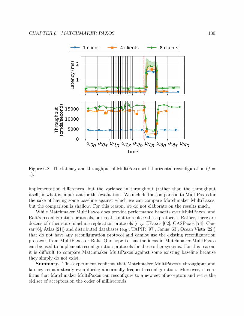
CHAPTER 6. MATCHMAKER PAXOS 130
1
2La
tenc
y (m
s)
0:00 0:05 0:10 0:15 0:20 0:25 0:30 0:35 0:40Time
0
5000
10000
15000
Thro
ughp
ut(c
mds
/sec
ond)
1 client 4 clients 8 clients
Figure 6.8: The latency and throughput of MultiPaxos with horizontal reconfiguration (f =1).
implementation differences, but the variance in throughput (rather than the throughputitself) is what is important for this evaluation. We include the comparison to MultiPaxos forthe sake of having some baseline against which we can compare Matchmaker MultiPaxos,but the comparison is shallow. For this reason, we do not elaborate on the results much.
While Matchmaker MultiPaxos does provide performance benefits over MultiPaxos’ andRaft’s reconfiguration protocols, our goal is not to replace these protocols. Rather, there aredozens of other state machine replication protocols (e.g., EPaxos [62], CASPaxos [74], Cae-sar [6], Atlas [21]) and distributed databases (e.g., TAPIR [97], Janus [63], Ocean Vista [22])that do not have any reconfiguration protocol and cannot use the existing reconfigurationprotocols from MultiPaxos or Raft. Our hope is that the ideas in Matchmaker MultiPaxoscan be used to implement reconfiguration protocols for these other systems. For this reason,it is difficult to compare Matchmaker MultiPaxos against some existing baseline becausethey simply do not exist.
Summary. This experiment confirms that Matchmaker MultiPaxos’s throughput andlatency remain steady even during abnormally frequent reconfiguration. Moreover, it con-firms that Matchmaker MultiPaxos can reconfigure to a new set of acceptors and retire theold set of acceptors on the order of milliseconds.
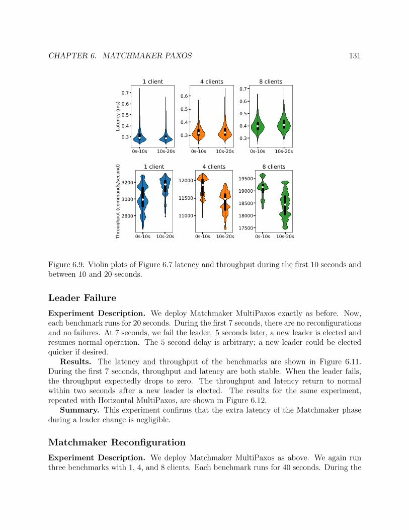
CHAPTER 6. MATCHMAKER PAXOS 131
0s-10s 10s-20s
0.3
0.4
0.5
0.6
0.7
Late
ncy
(ms)
1 client
0s-10s 10s-20s
0.3
0.4
0.5
0.6
4 clients
0s-10s 10s-20s
0.3
0.4
0.5
0.6
0.78 clients
0s-10s 10s-20s
2800
3000
3200
Thro
ughp
ut (c
omm
ands
/sec
ond) 1 client
0s-10s 10s-20s
11000
11500
12000
4 clients
0s-10s 10s-20s17500
18000
18500
19000
19500
8 clients
Figure 6.9: Violin plots of Figure 6.7 latency and throughput during the first 10 seconds andbetween 10 and 20 seconds.
Leader Failure
Experiment Description. We deploy Matchmaker MultiPaxos exactly as before. Now,each benchmark runs for 20 seconds. During the first 7 seconds, there are no reconfigurationsand no failures. At 7 seconds, we fail the leader. 5 seconds later, a new leader is elected andresumes normal operation. The 5 second delay is arbitrary; a new leader could be electedquicker if desired.
Results. The latency and throughput of the benchmarks are shown in Figure 6.11.During the first 7 seconds, throughput and latency are both stable. When the leader fails,the throughput expectedly drops to zero. The throughput and latency return to normalwithin two seconds after a new leader is elected. The results for the same experiment,repeated with Horizontal MultiPaxos, are shown in Figure 6.12.
Summary. This experiment confirms that the extra latency of the Matchmaker phaseduring a leader change is negligible.
Matchmaker Reconfiguration
Experiment Description. We deploy Matchmaker MultiPaxos as above. We again runthree benchmarks with 1, 4, and 8 clients. Each benchmark runs for 40 seconds. During the

CHAPTER 6. MATCHMAKER PAXOS 132
0s-10s 10s-20s0.18
0.20
0.22
0.24
0.26
0.28
Late
ncy
(ms)
1 client
0s-10s 10s-20s
0.20
0.25
0.30
0.35
4 clients
0s-10s 10s-20s0.2
0.3
0.4
0.5
0.6
0.7 8 clients
0s-10s 10s-20s
4200
4300
4400
4500
Thro
ughp
ut (c
omm
ands
/sec
ond) 1 client
0s-10s 10s-20s
13000
13500
14000
4 clients
0s-10s 10s-20s14000
15000
16000
17000
180008 clients
Figure 6.10: Violin plots of Figure 6.8 latency and throughput during the first 10 secondsand between 10 and 20 seconds.
first 10 seconds, there are no reconfigurations and no failures. Between 10 and 20 seconds,the leader reconfigures the set of matchmakers once every second. Every reconfigurationrandomly selects 2f+1 matchmakers from a set of 2×(2f+1) matchmakers. At 25 seconds,we fail a matchmaker. At 30 we perform a matchmaker reconfiguration to replace the failedmatchmaker. At 35 seconds, we reconfigure the acceptors.
Results. The latency and throughput of Matchmaker MultiPaxos are shown in Fig-ure 6.13. The latency and throughput of the protocol remain steady through the first tenmatchmaker reconfigurations, through the matchmaker failure and recovery, and through theacceptor reconfiguration. This is confirmed by the medians, IQRs, and standard deviationsof the latency and throughput during the first 10 seconds and between 10 and 20 seconds,which are shown in Table 6.2.
Summary. This benchmark confirms that matchmakers are off the critical path. Thelatency and throughput of Matchmaker MultiPaxos remains steady during a matchmakerreconfiguration and matchmaker failure. Moreover, a matchmaker reconfiguration does notaffect the performance of subsequent acceptor reconfigurations.

CHAPTER 6. MATCHMAKER PAXOS 133
Table 6.1: Figure 6.7 median, interquartile range, and standard deviation of latency andthroughput.
Latency (ms)
1 Client 4 Clients 8 Clients0s-10s 10s-20s 0s-10s 10s-20s 0s-10s 10s-20s
median 0.292 0.287 0.317 0.321 0.398 0.410IQR 0.040 0.026 0.029 0.036 0.036 0.039stdev 0.114 0.085 0.076 0.081 0.089 0.305
Throughput (commands/second)
1 Client 4 Clients 8 Clients0s-10s 10s-20s 0s-10s 10s-20s 0s-10s 10s-20s
median 2,995 3,177 11,874 11,478 19,146 18,446IQR 152 53 175 145 140 373stdev 157 111 298 307 358 520
6.6 Related Work
SMART. SMART [54] is a reconfiguration protocol that resolves many ambiguities in Mul-tiPaxos’ horizontal approach (e.g., when it is safe to retire old configurations). Like Multi-Paxos’ horizontal reconfiguration protocol, SMART can reconfigure a protocol with minimalperformance degradation. SMART differs from Matchmaker Paxos is a number of ways.First, like MultiPaxos’ horizontal reconfiguration protocol, SMART is fundamentally logbased and is therefore incompatible with many sophisticated state machine replication pro-tocols. Second, SMART assumes that acceptors and replicas are always co-located. Thisprevents us from reconfiguring the acceptors without reconfiguring the replicas. This is notideal since we can reconfigure an acceptor without copying any state, but must transfer logsfrom an old replica to a new replica. SMART’s garbage collection also has higher latencythat Matchmaker Paxos’ garbage collection. For Scenario 3, Matchmaker Paxos proposerswait until a prefix of the log is stored on f + 1 replicas. SMART waits for the prefix of thelog to be executed and snapshotted by f + 1 replicas.
Cheap Paxos. Cheap Paxos [50] is a MultiPaxos variant that consists of a fixed set off + 1 main acceptors and f auxiliary acceptors. During failure-free execution (the normalcase), only the main acceptors are contacted. The auxiliary acceptors perform MultiPaxos’horizontal reconfiguration protocol to replace failed main acceptors. As with Fast Paxos,we can deploy Matchmaker MultiPaxos with only f + 1 acceptors, f fewer than CheapPaxos. Matchmaker Paxos does require 2f + 1 matchmakers, but matchmakers do not actas acceptors and have to process only a single message (i.e. a MatchA message) to perform

CHAPTER 6. MATCHMAKER PAXOS 134
0.00.51.01.52.0
Late
ncy
(ms)
0:00 0:05 0:10 0:15 0:20Time
5000
10000
15000
Thro
ughp
ut(c
mds
/sec
ond)
1 client 4 clients 8 clients
Figure 6.11: Matchmaker MultiPaxos’ latency and throughput (f = 1). The dashed red linedenotes a leader failure.
a reconfiguration.Raft. Raft [68] uses a reconfiguration protocol called joint consensus. Like MultiPaxos’
horizontal reconfiguration, joint consensus is log-based and therefore incompatible with manyexisting replication protocols. A simpler reconfiguration protocol for Raft was proposedin [67] but requires more rounds of communication.
Viewstamped Replication (VR). VR [53] uses a stop-the-world approach to recon-figuration. During a reconfiguration, the entire protocol stops processing commands. Thus,while the reconfiguration is quite simple, it is inefficient. Stoppable Paxos [48] is similar toMultiPaxos’ horizontal reconfiguration, but also uses a stop-the-world approach. VR’s stop-the-world approach to reconfiguration is also adopted by databases built on VR, includingTAPIR [97] and Meerkat [82]. We use a similar approach to reconfigure matchmakers, butbecause matchmakers are off the critical path, the performance overheads are invisible.
Fast Paxos Coordinated Recovery. Fast Paxos has an optimization called coordi-nated recovery that is similar to Phase 1 Bypassing. The main difference is that in coordi-nated recovery, a leader uses Phase 2 information in round i to skip Phase 1 in round i+ 1,whereas with Phase 1 Bypassing, the leader instead uses Phase 1 information. Note thatcoordinated recovery is not useful for Matchmaker MultiPaxos. It is subsumed by Phase 1Bypassing. Coordinated recovery is only needed for Fast Paxos because the leader may notknow which values were proposed in a round it owns. Phase 1 Bypassing cannot be appliedto Fast Paxos for pretty much the same reason.
DynaStore. Vertical Paxos assumes its external master is implemented using state ma-

CHAPTER 6. MATCHMAKER PAXOS 135
0.00.51.01.52.0
Late
ncy
(ms)
0:00 0:05 0:10 0:15 0:20Time
5000
10000
15000
Thro
ughp
ut(c
mds
/sec
ond)
1 client 4 clients 8 clients
Figure 6.12: The latency and throughput of Horizontal MultiPaxos with f = 1.
chine replication. MultiPaxos’ horizontal reconfiguration also depends on consensus. Match-maker Paxos does not require consensus to implement matchmakers, but we are not the firstto notice this. DynaStore [3] showed that reconfiguring atomic storage does not requireconsensus.
ZooKeeper. ZooKeeper, a distributed coordinated service, which uses ZooKeeper AtomicBroadcast [36] is a protocol similar to MultiPaxos that can also reconfigure quickly afterleader failures.

CHAPTER 6. MATCHMAKER PAXOS 136
0.4
0.6
Late
ncy
(ms)
0:00 0:05 0:10 0:15 0:20 0:25 0:30 0:35Time
5000
10000
15000
20000
Thro
ughp
ut(c
mds
/sec
ond)
1 client 4 clients 8 clients
Figure 6.13: The latency and throughput of Matchmaker MultiPaxos (f = 1). The dottedblue, dashed red, and vertical black lines show matchmaker reconfigurations, a matchmakerfailure, and an acceptor reconfiguration respectively.
Table 6.2: Figure 6.13 median, interquartile range, and standard deviation of latency andthroughput.
Latency (ms)
1 Client 4 Clients 8 Clients0s-10s 10s-20s 0s-10s 10s-20s 0s-10s 10s-20s
median 0.297 0.292 0.314 0.313 0.404 0.398IQR 0.032 0.024 0.031 0.030 0.035 0.028stdev 0.077 0.061 0.093 0.098 0.383 0.067
Throughput (commands/second)
1 Client 4 Clients 8 Clients0s-10s 10s-20s 0s-10s 10s-20s 0s-10s 10s-20s
median 3019 3147 11631 11726 18569 19248IQR 41 51 140 145 391 71stdev 66 72 250 231 478 159

137
Chapter 7
Conclusion and Lessons Learned
In this thesis, we examined many facets of state machine replication. We compartmentalizedMultiPaxos to increase its throughput by over 10×. We enhanced and automated the under-lying theory of read-write quorum systems. We provided insight on a class of multi-leadergeneralized state machine replication protocols that were previously extremely challengingto understand. We designed a new reconfiguration protocol that provides theoretical in-sights and can be generalized to many protocols. Through this research, we have learnedthe following lessons.
State machine replication does not have to be slow The throughput of state machinereplication protocols reported in the literature varies tremendously. You’ll find papers withthroughput in the hundreds [31], in the tens of thousands [61], in the tens of millions [98],and in the billions [35] of commands per second. So while state machine replication protocolslike MultiPaxos can be slow if implemented in a straightforward way, our research and otherexisting research has shown that there are straightforward protocols that can be adopted andstraightforward protocol optimizations that can be used to achieve high throughput statemachine replication.
Practical aspects of consensus need more attention MultiPaxos is an old protocoland has received a lot of attention over many years, so naturally there are dozens of papersfocusing on improving very small details in the protocol. How can we shrink quorums byone node? How can we increase the likelihood of taking the fast path? This research isboth interesting and important, so its abundance is justified. Surprisingly though, thereis very little research on many practical aspects of state machine replication. How can wereconfigure a protocol? How do we garbage collect a protocol? What do we have to store ondisk and what can we store in memory? Answering these questions is vital for implementingstate machine replication in practice and deserves more attention.
Throughput and latency are very different goals Many state machine replicationprotocols aim to achieve high throughput and low latency in both the local and wide area

CHAPTER 7. CONCLUSION AND LESSONS LEARNED 138
network. However, we think that attempting to accomplish all these goals simultaneously ismisguided. For example, we can use compartmentalization to achieve very high throughputwithin a single data center. In performing these optimizations, we increase commit time,but within a data center, this doesn’t have a significant impact on latency. In the widearea, on the other hand, this increased commit time has a major impact on latency. Inthis setting, decreasing commit time is key. Unfortunately, decreasing commit time is amuch much more challenging task that requires very clever protocols. Protocols like FastPaxos [46], NOPaxos [51], SpecPaxos [71], and CURP [69] all reduce commit time and areall significantly more complicated than MultiPaxos. Ultimately, we believe that achievinghigh throughput within a data center is actually relatively straightforward, but achieving lowlatency in a wide area network is very complicated. Practitioners should pick the simplestprotocol that meets their needs.
Complex protocols can be understood given the right format and framing Pro-tocols like EPaxos [61], Caesar [6], and Atlas [21] are complex protocols. Explaining theseprotocols in a twelve page research paper is almost impossible. As a result, the protocols arepresented tersely and many explanations and proofs are pushed to appendices and technicalreports. The explanations are constrained by the publication format. Contrast this, forexample, with Lamport’s 36 page manuscript on Generalized Paxos [42]. Generalized Paxosis also a very complicated protocol, but Lamport is able to describe the protocol carefully.As another example, we believe our tutorial on generalized multi-leader protocols is theclearest and most comprehensive to date, but it’s impossible to fit the tutorial in a standardtwelve page paper. In summary, we believe that many protocols that are considered “toocomplicated” are more accurately “not able to be sufficiently explained given publishingconstraints.”
Automating compartmentalization The compartmentalizations performed in this dis-sertation were all done manually. Compartmentalization is intentionally straightforwardto the point of being almost mechanical, which makes it an attractive target for automa-tion. Distributed systems could be expressed in a high-level language like Bloom [5, 17] orTLA+ [96], and then a compiler could automatically identify opportunities for compartmen-talization. The optimizer could also determine the appropriate amount of decoupling andscaling to meet a certain optimization objective.
Extending beyond state machine replication In this dissertation, we applied com-partmentalization to state machine replication, but compartmentalization is a generally ap-plicable technique and can be applied to many other types of protocols. For example, there isongoing work to apply compartmentalization to Byzantine state machine replication proto-cols. Compartmentalization could also be applied to distributed model training, distributeddata processing systems, distributed databases, and so on.

139
Bibliography
[1] A Brief Introduction of TiDB. https://pingcap.github.io/blog/2017-05-23-perconalive17/. Accessed: 2019-10-21.
[2] Divyakant Agrawal and Amr El Abbadi. “The Tree Quorum Protocol: An EfficientApproach for Managing Replicated Data”. In: Proceedings of the 16th InternationalConference on Very Large Data Bases. VLDB ’90. San Francisco, CA, USA: MorganKaufmann Publishers Inc., 1990, pp. 243–254. isbn: 155860149X.
[3] Marcos K Aguilera et al. “Dynamic atomic storage without consensus”. In: Journal ofthe ACM (JACM) 58.2 (2011), pp. 1–32.
[4] Ailidani Ailijiang et al. “WPaxos: Wide Area Network Flexible Consensus”. In: IEEETransactions on Parallel and Distributed Systems (2019).
[5] Peter Alvaro et al. “Consistency Analysis in Bloom: a CALM and Collected Approach”.In: CIDR. Citeseer. 2011, pp. 249–260.
[6] Balaji Arun et al. “Speeding up Consensus by Chasing Fast Decisions”. In: 2017IEEE/IFIP International Conference on Dependable Systems & Networks (DSN). IEEE.2017, pp. 49–60.
[7] Berk Atikoglu et al. “Workload analysis of a large-scale key-value store”. In: Proceedingsof the 12th ACM SIGMETRICS/PERFORMANCE joint international conference onMeasurement and Modeling of Computer Systems. 2012, pp. 53–64.
[8] Johannes Behl, Tobias Distler, and Rudiger Kapitza. “Consensus-oriented paralleliza-tion: How to earn your first million”. In: Proceedings of the 16th Annual MiddlewareConference. ACM. 2015, pp. 173–184.
[9] Carlos Eduardo Bezerra, Fernando Pedone, and Robbert Van Renesse. “Scalable state-machine replication”. In: 2014 IEEE/IFIP International Conference on DependableSystems & Networks (DSN). IEEE. 2014, pp. 331–342.
[10] Martin Biely et al. “S-paxos: Offloading the leader for high throughput state machinereplication”. In: 2012 IEEE 31st Symposium on Reliable Distributed Systems (SRDS).IEEE. 2012, pp. 111–120.
[11] Mike Burrows. “The Chubby lock service for loosely-coupled distributed systems”. In:7th USENIX Symposium on Operating Systems Design and Implementation (OSDI06). 2006, pp. 335–350.

BIBLIOGRAPHY 140
[12] Tushar D Chandra, Robert Griesemer, and Joshua Redstone. “Paxos made live: anengineering perspective”. In: Proceedings of the 2007 ACM Symposium on Principlesof Distributed Computing. ACM. 2007, pp. 398–407.
[13] Aleksey Charapko, Ailidani Ailijiang, and Murat Demirbas. “Linearizable quorumreads in Paxos”. In: 11th USENIX Workshop on Hot Topics in Storage and File Sys-tems (HotStorage 19). 2019.
[14] Aleksey Charapko, Ailidani Ailijiang, and Murat Demirbas. “PigPaxos: Devouringthe communication bottlenecks in distributed consensus”. In: Proceedings of the 2021International Conference on Management of Data. ACM. 2021, pp. 235–247.
[15] Shun Yan Cheung, Mustaque Ahamad, and Mostafa H. Ammar. “Multidimensionalvoting: a general method for implementing synchronization in distributed systems”. In:Proceedings of the 10th International Conference on Distributed Computing Systems.May 1990, pp. 362–369. doi: 10.1109/ICDCS.1990.89304.
[16] Shun Yan Cheung, Mostafa H. Ammar, and Mustaque Ahamad. “The Grid Protocol:A High Performance Scheme for Maintaining Replicated Data”. In: IEEE Trans. onKnowl. and Data Eng. 4.6 (Dec. 1992), pp. 582–592. issn: 1041-4347. doi: 10.1109/69.180609. url: https://doi.org/10.1109/69.180609.
[17] Neil Conway et al. “Logic and lattices for distributed programming”. In: Proceedingsof the Third ACM Symposium on Cloud Computing. 2012, pp. 1–14.
[18] James C Corbett et al. “Spanner: Google’s globally distributed database”. In: ACMTransactions on Computer Systems (TOCS) 31.3 (2013), p. 8.
[19] Giuseppe DeCandia et al. “Dynamo: Amazon’s highly available key-value store”. In:ACM SIGOPS operating systems review 41.6 (2007), pp. 205–220.
[20] Cong Ding et al. “Scalog: Seamless Reconfiguration and Total Order in a ScalableShared Log”. In: 17th USENIX Symposium on Networked Systems Design and Imple-mentation (NSDI 20). 2020, pp. 325–338.
[21] Vitor Enes et al. “State-machine replication for planet-scale systems”. In: Proceedingsof the Fifteenth European Conference on Computer Systems. 2020, pp. 1–15.
[22] Hua Fan and Wojciech Golab. “Ocean vista: gossip-based visibility control for speedygeo-distributed transactions”. In: Proceedings of the VLDB Endowment 12.11 (2019),pp. 1471–1484.
[23] Michael J Fischer, Nancy A Lynch, and Michael S Paterson. “Impossibility of dis-tributed consensus with one faulty process”. In: Journal of the ACM (JACM) 32.2(1985), pp. 374–382.
[24] Hector Garcia-Molina and Daniel Barbara. “How to Assign Votes in a DistributedSystem”. In: J. ACM 32.4 (Oct. 1985), pp. 841–860. issn: 0004-5411. doi: 10.1145/4221.4223. url: https://doi.org/10.1145/4221.4223.
BIBLIOGRAPHY 141
[25] Sanjay Ghemawat, Howard Gobioff, and Shun-Tak Leung. “The Google file system”.In: Proceedings of the 19th Symposium on Operating Systems Principles. ACM. 2003,pp. 29–43.
[26] David K. Gifford. “Weighted Voting for Replicated Data”. In: Proceedings of the Sev-enth ACM Symposium on Operating Systems Principles. SOSP ’79. New York, NY,USA: Association for Computing Machinery, 1979, pp. 150–162. isbn: 0897910095.doi: 10.1145/800215.806583. url: https://doi.org/10.1145/800215.806583.
[27] Global data distribution with Azure Cosmos DB - under the hood. https://docs.microsoft.com/en-us/azure/cosmos-db/global-dist-under-the-hood. Ac-cessed: 2019-10-21.
[28] Maurice P Herlihy and Jeannette M Wing. “Linearizability: A correctness condition forconcurrent objects”. In: ACM Transactions on Programming Languages and Systems(TOPLAS) 12.3 (1990), pp. 463–492.
[29] Heidi Howard. “Distributed consensus revised”. PhD thesis. University of Cambridge,2019.
[30] Heidi Howard, Aleksey Charapko, and Richard Mortier. “Fast Flexible Paxos: Relax-ing Quorum Intersection for Fast Paxos”. In: International Conference on DistributedComputing and Networking 2021. 2021, pp. 186–190.
[31] Heidi Howard, Dahlia Malkhi, and Alexander Spiegelman. “Flexible Paxos: QuorumIntersection Revisited”. In: 20th International Conference on Principles of DistributedSystems (OPODIS 2016). Schloss Dagstuhl-Leibniz-Zentrum fuer Informatik. 2017.
[32] Heidi Howard, Dahlia Malkhi, and Alexander Spiegelman. “Flexible Paxos: QuorumIntersection Revisited”. In: 20th International Conference on rinciples of DistributedSystems (OPODIS 2016). Ed. by Panagiota Fatourou, Ernesto Jimenez, and FernandoPedone. Vol. 70. Leibniz International Proceedings in Informatics (LIPIcs). Dagstuhl,Germany: Schloss Dagstuhl–Leibniz-Zentrum fuer Informatik, 2017, 25:1–25:14. isbn:978-3-95977-031-6. doi: 10.4230/LIPIcs.OPODIS.2016.25. url: http://drops.dagstuhl.de/opus/volltexte/2017/7094.
[33] Heidi Howard and Richard Mortier. “Paxos vs Raft: Have we reached consensus ondistributed consensus?” In: Proceedings of the 7th Workshop on Principles and Practiceof Consistency for Distributed Data. 2020, pp. 1–9.
[34] Toshihide Ibaraki and Tiko Kameda. “A theory of coteries: Mutual exclusion in dis-tributed systems”. In: IEEE Transactions on Parallel and Distributed Systems 4.7(1993), pp. 779–794.
[35] Xin Jin et al. “Netchain: Scale-free sub-rtt coordination”. In: 15th USENIX Symposiumon Networked Systems Design and Implementation (NSDI 18). 2018, pp. 35–49.
[36] Flavio P Junqueira, Benjamin C Reed, and Marco Serafini. “Zab: High-performancebroadcast for primary-backup systems”. In: 2011 IEEE/IFIP 41st International Con-ference on Dependable Systems & Networks (DSN). IEEE. 2011, pp. 245–256.

BIBLIOGRAPHY 142
[37] Manos Kapritsos and Flavio Paiva Junqueira. “Scalable Agreement: Toward Orderingas a Service”. In: HotDep. 2010.
[38] Kubernetes. Kubernetes. https://kubernetes.io. accessed: 2020-03-01.
[39] Akhil Kumar. “Hierarchical Quorum Consensus: A New Algorithm for Managing Repli-cated Data”. In: IEEE Trans. Comput. 40.9 (Sept. 1991), pp. 996–1004. issn: 0018-9340. doi: 10.1109/12.83661. url: https://doi.org/10.1109/12.83661.
[40] Avinash Lakshman and Prashant Malik. “Cassandra: a decentralized structured stor-age system”. In: ACM SIGOPS Operating Systems Review 44.2 (2010), pp. 35–40.
[41] Leslie Lamport. “Fast paxos”. In: Distributed Computing 19.2 (2006), pp. 79–103.
[42] Leslie Lamport. “Generalized consensus and Paxos”. In: (2005).
[43] Leslie Lamport. “How to make a multiprocessor computer that correctly executes mul-tiprocess progranm”. In: IEEE Transactions on Computers 9 (1979), pp. 690–691.
[44] Leslie Lamport. “Paxos made simple”. In: ACM Sigact News 32.4 (2001), pp. 18–25.
[45] Leslie Lamport. “The part-time parliament”. In: ACM Transactions on Computer Sys-tems (TOCS) 16.2 (1998), pp. 133–169.
[46] Leslie Lamport. “Time, clocks, and the ordering of events in a distributed system”. In:Concurrency: the Works of Leslie Lamport. 2019, pp. 179–196.
[47] Leslie Lamport, Dahlia Malkhi, and Lidong Zhou. “Reconfiguring a state machine.”In: SIGACT News 41.1 (2010), pp. 63–73.
[48] Leslie Lamport, Dahlia Malkhi, and Lidong Zhou. “Stoppable paxos”. In: TechReport,Microsoft Research (2008).
[49] Leslie Lamport, Dahlia Malkhi, and Lidong Zhou. “Vertical paxos and primary-backupreplication”. In: Proceedings of the 28th ACM symposium on Principles of distributedcomputing. 2009, pp. 312–313.
[50] Leslie Lamport and Mike Massa. “Cheap paxos”. In: International Conference on De-pendable Systems and Networks, 2004. IEEE. 2004, pp. 307–314.
[51] Jialin Li et al. “Just Say NO to Paxos Overhead: Replacing Consensus with NetworkOrdering”. In: 12th USENIX Symposium on Operating Systems Design and Implemen-tation (OSDI 16). 2016, pp. 467–483.
[52] Lightweight transactions in Cassandra 2.0. https://www.datastax.com/blog/2013/07/lightweight-transactions-cassandra-20. Accessed: 2019-10-21.
[53] Barbara Liskov and James Cowling. “Viewstamped replication revisited”. In: (2012).
[54] Jacob R Lorch et al. “The SMART way to migrate replicated stateful services”. In:Proceedings of the 1st ACM SIGOPS/EuroSys European Conference on Computer Sys-tems 2006. 2006, pp. 103–115.

BIBLIOGRAPHY 143
[55] Giuliano Losa, Sebastiano Peluso, and Binoy Ravindran. “Brief announcement: A fam-ily of leaderless generalized-consensus algorithms”. In: Proceedings of the 2016 ACMSymposium on Principles of Distributed Computing. ACM. 2016, pp. 345–347.
[56] Mamoru Maekawa. “A square root N Algorithm for Mutual Exclusion in DecentralizedSystems”. In: ACM Trans. Comput. Syst. 3.2 (May 1985), pp. 145–159. issn: 0734-2071.doi: 10.1145/214438.214445. url: https://doi.org/10.1145/214438.214445.
[57] Yanhua Mao, Flavio P Junqueira, and Keith Marzullo. “Mencius: building efficientreplicated state machines for WANs”. In: 8th USENIX Symposium on Operating Sys-tems Design and Implementation (OSDI 08). 2008, pp. 369–384.
[58] Parisa Jalili Marandi et al. “Ring Paxos: A high-throughput atomic broadcast pro-tocol”. In: 2010 IEEE/IFIP International Conference on Dependable Systems & Net-works (DSN). IEEE. 2010, pp. 527–536.
[59] David Mazieres. “Paxos made practical”. In: Unpublished manuscript, Jan (2007).
[60] Iulian Moraru, David G Andersen, and Michael Kaminsky. A proof of correctness forEgalitarian Paxos. Tech. rep. Technical report, Parallel Data Laboratory, CarnegieMellon University, 2013.
[61] Iulian Moraru, David G Andersen, and Michael Kaminsky. “Paxos quorum leases: Fastreads without sacrificing writes”. In: Proceedings of the ACM Symposium on CloudComputing. 2014, pp. 1–13.
[62] Iulian Moraru, David G Andersen, and Michael Kaminsky. “There is more consensus inegalitarian parliaments”. In: Proceedings of the 24th Symposium on Operating SystemsPrinciples. ACM. 2013, pp. 358–372.
[63] Shuai Mu et al. “Consolidating concurrency control and consensus for commits underconflicts”. In: 12th USENIX Symposium on Operating Systems Design and Implemen-tation (OSDI 16). 2016, pp. 517–532.
[64] Moni Naor and Avishai Wool. “The Load, Capacity, and Availability of Quorum Sys-tems”. In: SIAM Journal on Computing 27.2 (1998). issn: 0097-5397. doi: 10.1137/S0097539795281232. url: https://doi.org/10.1137/S0097539795281232.
[65] Faisal Nawab, Divyakant Agrawal, and Amr El Abbadi. “Dpaxos: Managing data closerto users for low-latency and mobile applications”. In: Proceedings of the 2018 Interna-tional Conference on Management of Data. ACM. 2018, pp. 1221–1236.
[66] Rajesh Nishtala et al. “Scaling memcache at facebook”. In: 10th USENIX Symposiumon Networked Systems Design and Implementation (NSDI 13). 2013, pp. 385–398.
[67] Diego Ongaro. “Consensus: Bridging theory and practice”. PhD thesis. Stanford Uni-versity, 2014.
[68] Diego Ongaro and John K Ousterhout. “In search of an understandable consensusalgorithm”. In: USENIX Annual Technical Conference. 2014, pp. 305–319.

BIBLIOGRAPHY 144
[69] Seo Jin Park and John Ousterhout. “Exploiting commutativity for practical fast repli-cation”. In: 16th USENIX Symposium on Networked Systems Design and Implemen-tation (NSDI 19). 2019, pp. 47–64.
[70] David Peleg and Avishai Wool. “Crumbling Walls: A Class of Practical and EfficientQuorum Systems”. In: Proceedings of the Fourteenth Annual ACM Symposium on Prin-ciples of Distributed Computing. PODC ’95. Ottowa, Ontario, Canada: Association forComputing Machinery, 1995, pp. 120–129. isbn: 0897917103. doi: 10.1145/224964.224978. url: https://doi.org/10.1145/224964.224978.
[71] Dan RK Ports et al. “Designing Distributed Systems Using Approximate Synchrony inData Center Networks”. In: 12th USENIX Symposium on Networked Systems Designand Implementation (NSDI 15). 2015, pp. 43–57.
[72] Raft Replication in YugaByte DB. https://www.yugabyte.com/resources/raft-replication-in-yugabyte-db/. Accessed: 2019-10-21.
[73] Sajjad Rizvi, Bernard Wong, and Srinivasan Keshav. “Canopus: A scalable and mas-sively parallel consensus protocol”. In: Proceedings of the 13th International Conferenceon emerging Networking EXperiments and Technologies. 2017, pp. 426–438.
[74] Denis Rystsov. “CASPaxos: Replicated State Machines without logs”. In: arXiv preprintarXiv:1802.07000 (2018).
[75] Nuno Santos and Andre Schiper. “Achieving high-throughput state machine replicationin multi-core systems”. In: 2013 IEEE 33rd International Conference on DistributedComputing Systems. Ieee. 2013, pp. 266–275.
[76] Nuno Santos and Andre Schiper. “Optimizing Paxos with batching and pipelining”.In: Theoretical Computer Science 496 (2013), pp. 170–183.
[77] Nuno Santos and Andre Schiper. “Tuning paxos for high-throughput with batching andpipelining”. In: International Conference on Distributed Computing and Networking.Springer. 2012, pp. 153–167.
[78] Fred B Schneider. “Implementing fault-tolerant services using the state machine ap-proach: A tutorial”. In: ACM Computing Surveys (CSUR) 22.4 (1990), pp. 299–319.
[79] William Schultz, Tess Avitabile, and Alyson Cabral. “Tunable Consistency in Mon-goDB”. In: Proceedings of the VLDB Endowment 12.12 (2019), pp. 2071–2081.
[80] Rong Shi and Yang Wang. “Cheap and available state machine replication”. In: 2016USENIX Annual Technical Conference (USENIXATC 16). 2016, pp. 265–279.
[81] Pierre Sutra and Marc Shapiro. “Fast genuine generalized consensus”. In: 2011 IEEE30th Symposium on Reliable Distributed Systems (SRDS). IEEE. 2011, pp. 255–264.
[82] Adriana Szekeres et al. “Meerkat: Multicore-Scalable Replicated Transactions Follow-ing the Zero-Coordination Principle”. In: Proceedings of the Fourteenth EuroSys Con-ference 2020. 2020.

BIBLIOGRAPHY 145
[83] Rebecca Taft et al. “CockroachDB: The Resilient Geo-Distributed SQL Database”.In: Proceedings of the 2020 International Conference on Management of Data. ACM.2020, pp. 1493–1509.
[84] Hatem Takruri et al. “FLAIR: Accelerating Reads with Consistency-Aware NetworkRouting”. In: 17th USENIX Symposium on Networked Systems Design and Implemen-tation (NSDI 20). 2020, pp. 723–737.
[85] Jeff Terrace and Michael J Freedman. “Object Storage on CRAQ: High-ThroughputChain Replication for Read-Mostly Workloads”. In: USENIX Annual Technical Con-ference. June. San Diego, CA. 2009, pp. 1–16.
[86] Alexander Thomson et al. “Calvin: fast distributed transactions for partitioned databasesystems”. In: Proceedings of the 2012 International Conference on Management ofData. ACM. 2012, pp. 1–12.
[87] Robbert Van Renesse and Deniz Altinbuken. “Paxos made moderately complex”. In:ACM Computing Surveys (CSUR) 47.3 (2015), p. 42.
[88] Robbert Van Renesse and Fred B Schneider. “Chain Replication for Supporting HighThroughput and Availability”. In: 6th USENIX Symposium on Operating Systems De-sign and Implementation (OSDI 04). Vol. 4. 91–104. 2004.
[89] Matt Welsh, David Culler, and Eric Brewer. “SEDA: an architecture for well-conditioned,scalable internet services”. In: ACM SIGOPS Operating Systems Review. Vol. 35. 5.ACM. 2001, pp. 230–243.
[90] Michael Whittaker and Joseph M Hellerstein. “Checking Invariant Confluence, InWhole or In Parts”. In: ACM SIGMOD Record 49.1 (2020), pp. 7–14.
[91] Michael Whittaker and Joseph M Hellerstein. “Interactive checks for coordinationavoidance”. In: Proceedings of the VLDB Endowment 12.1 (2018), pp. 14–27.
[92] Michael Whittaker et al. “Debugging distributed systems with why-across-time prove-nance”. In: Proceedings of the ACM Symposium on Cloud Computing. 2018, pp. 333–346.
[93] Michael Whittaker et al. “Online template induction for machine-generated emails”.In: Proceedings of the VLDB Endowment 12.11 (2019), pp. 1235–1248.
[94] Michael Whittaker et al. “Read-Write Quorum Systems Made Practical”. In: Proceed-ings of the 8th Workshop on Principles and Practice of Consistency for DistributedData. 2021, pp. 1–8.
[95] Michael Whittaker et al. Scaling Replicated State Machines with Compartmentalization[Technical Report]. 2020. arXiv: 2012.15762 [cs.DC].
[96] Yuan Yu, Panagiotis Manolios, and Leslie Lamport. “Model checking TLA+ specifica-tions”. In: Advanced Research Working Conference on Correct Hardware Design andVerification Methods. Springer. 1999, pp. 54–66.

BIBLIOGRAPHY 146
[97] Irene Zhang et al. “Building consistent transactions with inconsistent replication”. In:ACM Transactions on Computer Systems (TOCS) 35.4 (2018), p. 12.
[98] Hang Zhu et al. “Harmonia: Near-linear scalability for replicated storage with in-network conflict detection”. In: Proceedings of the VLDB Endowment 13.3 (2019),pp. 376–389.