COMPARISON STUDY OF SORTING TECHNIQUES IN DYNAMIC

COMPARISON STUDY OF SORTING TECHNIQUES IN DYNAMIC DATA

STRUCTURE

ZEYAD ADNAN ABBAS

A dissertation submitted in

partial fulfilment of the requirement for the award of the

Degree of Master of Computer Science (Software Engineering)

Faculty of Computer Science and Information Technology

Universiti Tun Hussein Onn Malaysia

MARCH 2016

v

ABSTRACT

Sorting is an important and widely studied issue, where the execution time and the

required resources for computation is of extreme importance, especially if it is dealing

with real-time data processing. Therefore, it is important to study and to compare in

details all the available sorting algorithms. In this project, an intensive investigation was

conducted on five algorithms, namely, Bubble Sort, Insertion Sort, Selection Sort,

Merge Sort and Quick Sort algorithms. Four groups of data elements were created for

the purpose of comparison process among the different sorting algorithms. All the five

sorting algorithms are applied to these groups. The worst time complexity for each

sorting technique is then computed for each sorting algorithm. The sorting algorithms

were classified into two groups of time complexity, O (n2) group and O(nlog2n) group.

The execution time for the five sorting algorithms of each group of data elements were

computed. The fastest algorithm is then determined by the estimated value for each

sorting algorithm, which is computed using linear least square regression. The results

revealed that the Merge Sort was more efficient to sort data from the Quick Sort for

O(nlog2n) time complexity group. The Insertion Sort had more efficiency to sort data

from Selection Sort and Bubble Sort for O (n2) group. Bubble Sort was the slowest or it

was less efficient to sort the data. In conclusion, the efficiency of sorting algorithms can

be ranked from highest to lowest as Merge Sort, Quick Sort, Insertion Sort, Selection

Sort and Bubble Sort.

vi

ABSTRAK

Isihan merupakan satu masalah yang penting dan telah dikaji secara meluas, di mana

masa pelaksanaan dan sumber yang diperlukan untuk membuat pengiraan adalah sangat

penting, terutamanya dalam memproses data masa nyata. Oleh itu, ia adalah penting

untuk mengkaji dan membandingkan dengan terperinci semua algoritma isihan yang

ada. Dalam projek ini, kajian terperinci dijalankan ke atas lima algoritma sisihan, iaitu

Bubble Sort, Insertion Sort, Selection Sort, Merge Sort dan Quick Sort. Empat kumpulan

elemen data telah dibentuk untuk membuat perbandingan antara algoritma isihan yang

berbeza. Kesemua lima algoritma isihan digunakan kepada kumpulan elemen data ini.

Kekompleksan masa bagi setiap algoritma isihan telah dikira. Algoritma isihan

dikelaskan kepada dua kumpulan kekompleksan masa iaitu kumpulan O(n2) dan

kumpulan O(log2n). Masa pelaksanaan bagi lima algoritma isihan untuk setiap kempulan

elemen data telah dikira. Algoritma terpantas kemudian ditentukan menggunakan

anggaran nilai untuk setiap algoritma sisihan, yang dikira menggunakan linear least

square regression. Keputusan menunjukkan bahawa Merge Sort lebih pantas untuk

menyusun data daripada Quick Sort untuk kumpulan kekompleksan masa O(nlog2n).

Insertion Sort lebih cekap untuk menyusun data daripada Selection Sort dan Bubble Sort

untuk kumpulan kekompleksan masa O(n2). Manakala Bubble Sort mengambil masa

paling lama atau paling kurang cekap untuk menyusun data. Kesimpulannya, kecekapan

algoritma sisihan boleh disusun mengikut tahap yang paling cekap kepada kurang cekap

sebagai Merge Sort, Quick Sort, Insertion Sort, Selection Sort dan Bubble Sort.

vii

CONTENTS

TITLE i

DECLARATION ii

DEDICATION iii

ACKNOWLEDGEMENT iv

ABSTRACT v

ABSTRAK vi

CONTENTS vii

LIST OF TABLES x

LIST OF FIGURES xi

LIST OF APPENDICES xvi

CHAPTER 1 INTRODUCTION 2

1.1 Background 2

1.2 Problem Statement 3

1.3 Research Objectives 3

1.4 Research Scope 4

1.5 Outline of Report 4

1.6 Chapter Summary 5

CHAPTER 2 LITERATURE REVIEW 6

2.1 Introduction 6

2.2 Data Structure 6

2.2.1 Advantages of Linked list 8

2.2.2 Disadvantages of Linked list 8

2.3 Sorting Techniques 9

2.3.1 Selection Sort 9

2.3.2 Insertion Sort 11

viii

2.3.3 Bubble Sort 13

2.3.4 Quick Sort 14

2.3.5 Merge Sort 16

2.4 Time Complexity 18

2.4.1 Asymptotic notation 18

2.4.2 Big-O Notation 19

2.4.3 Running Time Analysis 19

2.4.4 Computational Complexity 21

2.4.5 Divide-and-conquer Algorithms 21

2.5 Regression 22

2.5.1 Linear regression 22

2.5.2 Simple linear regression using a single

predictor X 23

2.5.3 Estimation of the parameters by least squares 23

2.6 Related work 25


CHAPTER 3 METHODOLOGY 35

3.1 Introduction 35

3.2 Methodology 35

3.2.1 Phase 1: Create data group and Insert

to Linked list 37

3.3.2 Phase 2: Applying Sorting Techniques

and Calculate Time Complexity 40

3.3.3 Phase 3: Comparison of Sorting Techniques 44


CHAPTER 4 IMPLEMENTATION AND COMPARISON 48

4.1 Introduction 48

4.2 Implementation of Sorting Techniques 49

4.2.1 Bubble Sort Implementation 51

4.2.2 Insertion Sort Implementation 61

4.2.3 Implementation of Selection Sort 69

ix

4.2.4 Implementation of Merge Sort 78

4.2.5 Implementation of Quick Sort 86

4.3 Time Complexity Implementation 93

4.3.1 Bubble Sort Time Complexity 95

4.3.2 Insertion Sort Time Complexity 96

4.3.3 Selection Sort Time Complexity 97

4.3.4 Merge Sort Time Complexity 98

4.3.5 Quick Sort Time Complexity 100

4.3.6 Creat File Worst Case Time Complexity 102

4.3.7 Insert data to the Linked list Time Complexity 103

4.4 Execution Time for Sorting Techniques 105

4.4.1 Sorting Techniques Estimated

Values Comparison 109

4.5 Result and Conclusion 115


CHAPTER 5 CONCLUSIONS 116

5.1 Introduction 116

5.2 Objectives Achievement 116

5.4 Future Work 118

5.5 Project Contribution 118


REFERENCES 119

APPENDIX 123

VITA

x

LIST OF TABLES

2.1 Running Time for n = 100 to 1000 (Shene, 1996) 25

2.2 Running Time for n = 2000 to 10000 (Shene, 1996) 26

2.3 Constant Factors (Shene, 1996) 26

2.4 Running Time for Integer and String

(Aliyu and Zirra, 2013) 29

2.5 Related work summary 29

3.1 Files of Group1 38

3.2 File of Group2 39




4.1 Bubble Sort Execution Time Group1 Results 52

4.2 Bubble Sort Execution Time for Group2 55



4.5 Insertion Sort Execution Time Group1 61

4.6 Insertion Sort Execution Time Group2 Results 64



4.9 Selection Sort Execution Time Group1 Results 70




4.13 Merge Sort Execution Time Group1 Results 78

xi




4.17 Quick Sort Execution Time Group1 Results 86




4. 21 n2 and nlog2n big O notations groups 93

4.22 Create Files Groups 103

4.23 Sorting techniques execution time Group1 results 105

4.24 Sorting techniques execution time Group2 results 106

4.25 Sorting techniques execution time group3 107

4.26 Sorting techniques execution time Group4 108

4.27 Constant factors 110

4.28 Sorting Comparison per groups estimated values 112

4.29 Constant Factors Average 113

4.30 Sorting techniques Comparison 114

4. 31 Sorting Techniques 114

xii

LIST OF FIGURES

2.1 Structure of node 7

2.2 Linked list example 8

2.3 List of 9 elements 10

2.4 First Iteration for Selection Sort 10

2.5 Second Iteration for Selection Sort 11

2.6 Insertion Sort Example 12

2.7 Bubble Sort examples 13

2.8 Quick Sort Examples 15

2.9 Merge Sort Examples 17

2.10 Nested loop Example 20

2.11 Nested loop program 20

2.12 Linear regression example 22

2.13 Linear Least Square regression example 24

2.14 Execution Time for Negative Sequence

(Rao and Ramesh, 2012) 27

2.15 Execution Time for Positive Sequence

(Rao and Ramesh, 2012) 28

3.1 Research Methodology Flow Chart 36

3.2 File Algorithm 37

3.3 Create File Algorithm 38

3.4 Insertion Sort Algorithm 41

3.5 Selection Sort Algorithm 41

3.6 Bubble Sort algorithm 42

3.7 Quick Sort algorithm 42

xiii

3.8 Partitioning Procedure 43

3.9 Merge Sort Algorithm 43

4.1 menu function 49

4.2 Switch - Case Men 50

4.3 Showlist Function 51




4.7 Bubble Sort Execution Time For Group4 60





4.12 Selection Sort Execution Time Group1 71

4.13 Selection Sort Execution Time Group2 73



4. 16 Merge Sort Execution Time Group1 Results 79



4.19 Merge Sort Execution Time Group 4 Results 85




4.23 nlog2n big O notation 94

4.24 n2 big O notation 94

4.25 Bubble Sort program and time complexity 96

4.26 Insertion Sort Program and Time Complexity 97

4.27 Selection Sort program and Time Complexity 98

xiv

4.28 Merge Sort Program and Time Complexity 99

4.29 FrontBackSplit Function 99

4.30 SortededMerge Function 100

4.31 ListLength Function 101

4.32 Quick Sort Program and Time Complexity 102

4.33 Create File Program Time Complexity 103

4.34 Insert data to the Linked lists Program Time

Complexity 104

4.35 insert function program 104


4.37 Sorting Techniques Execution Time Group2 107



4.40 Sorting Techniques Stability 111

4.41 The Average of Sorting techniques estimated

Values 113

xv

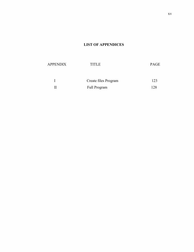
LIST OF APPENDICES

APPENDIX TITLE PAGE

I Create files Program 123

II Full Program 128

CHAPTER 1

INTRODUCTION

1.1 Background

Sorting is any process of arranging items in any sequence to reduce the cost of accessing

the data. Sorting techniques can be divided in two categories; comparison sorting

technique and non-comparison sorting techniques. A comparison sort is a type of sorting

algorithms that only reads the list of elements through a single abstract comparison

operation that determines which two elements should occur first in the final sorted list.

Comparison sorting consists of Bubble Sort, Insertion Sort, and Quick Sort. Non-

comparison sorting technique does not compare data elements in order to sort them. This

category includes Bucket Sort and Count Sort (Verma, & Kumar, 2013). The sorting

algorithm is used to rearrange the items of a given list in any order. Though dozens of

sorting algorithm have been developed, no single sorting technique is best suited for all

applications. Great research went into this category of algorithm because of its

importance. These types of algorithm are very much used in many computer algorithms.

For instance, searching an element, database algorithm and many more. Sorting

algorithm can be classified into two categories, internal sorting and external sorting. In

internal sorting all items to be sorted are kept in the main memory. External sorting, on

the other hand, deals with a large number of items, hence have resided in auxiliary

storage devices such as tape or disk (Dutta, 2013).

Weiss (2003) stressed on the importance of sorting. For instance, the words in a

dictionary must be sorted and case distinctions must be ignored. The files in a directory

must be listed in sorting order. The index of a book must be sorted and case distinctions

must ignored. Card catalog in a library must be sorted by both author and title. A listing

2

of course offerings at a university must be sorted, first by department and then by course

number. Many banks provide statements that list cheques in increasing order by cheque

number. In a newspaper, the calendar of events in a schedule is generally sorted by date.

The musical compact disks in a record store are generally sorted by recording artist. In

the programs printed for graduation ceremonies, departments are listed in sorted order

and then students in those departments are listed in sorted order.

Many computer scientists consider sorting to be a fundamental problem in the

study of algorithms. There are several reasons (Cormen et al., 2009). First, sometimes

they need to sort information that is inherent to an application. For example, in order to

prepare customer statements, the bank needs to sort cheques by cheque number. Second,

the algorithms often use sorting as a key subroutine. For example, a program that

renders graphical objects that are layered on top of each other might have to shoot the

object according to the layered relation so that it can draw these objects from bottom to

top. Third, sorting is a problem for which can achieve a nontrivial lower bound. The best

upper bound must match with lower bound asymptotically so know that the sorting

algorithm is optimal. Fourth, there are a wide variety of sorting algorithms and they use

various techniques. In fact, there are many important techniques used throughout the

algorithm design that have been developed over the years. Therefore, sorting is a

problem of historical interest. Previously, many engineering issues come to the fore

when they are implementing sorting algorithms. The fastest sorting program for a

particular situation may depend upon many factors, such as prior knowledge about the

keys and data, the memory hierarchy of the host computer and the software

environment.

The linked list data structure is one of the dynamic data structure methods that

are used to store the data. The linked list is the data structure used to save unsorted

elements and it was used from the sorting techniques namely, Bubble Sort, Insertion

Sort, Selection Sort, Merge Sort and Quick Sort to create a sorted linked list.

Thus, this study was comparing the sorting techniques according to worst case

time complexity and sorting execution time results.

3

1.2 Problem Statement

Sorting is the most fundamental algorithmic problem in computer science and a rich

source of programming problems for two distinct reasons. First, sorting is a useful

operation which efficiently solves many tasks that every programmer encounters.

Second, literally dozens of different sorting algorithms have been developed, each of

which rests on a particular clever idea or observation (Swain et al., 2013). Therefore, it

is essential to compare the prominent of sorting algorithm that is used in recent

technology. Today, rapid technology has enhanced the requirement for data processing

to meet the demand of the next era. Internet of things (IOT) (Vermesan, & Friess, 2013)

is one of the factors that increased the row of data significantly. Therefore, it is

important to use a sorting algorithm efficiently. However, it is unknown which

algorithm provides the optimum result, considering the required execution time for each

algorithm. This research was compare sorting algorithms in order to decide the proper

algorithm to avoid the hardware requirement which saves time and reduced the cost

significantly. Bubble Sort, Insertion Sort, Selection Sort, Quick Sort and Merge Sort are

a sample of sorting techniques that were compared in the research to determine which

sorting techniques that are sufficient to sort different sizes of data. In this research, the

difference, similarity and working for these sorting techniques was explained in details.

1.3 Research Objectives

The objectives of this project are to:

(i) implement Selection Sort, Insertion Sort, Bubble Sort, Quick Sort and Merge

sort using dynamic data structure (Linked list).

(ii) apply four groups of data elements into those techniques in (i).

(iii) calculate the time complexity, such as the execution time and worst case time

complexity.

4

1.4 Research Scope

This study focuses on the problem of sorting of many data sizes to determine which

sorting technique provides a result faster than other techniques in terms of the execution

time. They are grouped into:

(i) first group from 100 to 1000 data elements

(ii) second group from 2000 to 10000 data elements

(iii) third group from 11000 to 20000 data elements

(iv) fourth group from 21000 to 30000 data elements

A linked list dynamic data structure is used to store the data. Five Sorting algorithms are

used, namely, Selection Sort, Insertion Sort, Bubble Sort, Merge Sort and Quick Sort.

The execution time is the criteria used to discuss the performance of these sorting

algorithms. The Visual C++ program is used to implement the sorting algorithm

program and calculate the execution time for all sorting algorithms.

1.5 Outline of Report

This research consists of five chapters. Chapter 1 covers the overview and main

objectives of the research. It also consists of the scope of work covered. Chapter 2

illustrates the Selection Sort and Insertion Sort, Merge Sort, Quick Sort and Bubble Sort.

This chapter focus on literature review and related works of the research. Chapter 3

discusses the methodology used to achieve the entire objectives of this research. Chapter

4 explains the implementation and the detailed steps as well as the results and

discussion. Finally, Chapter 5 illustrates objectives achieved, future work and conclusion

.

5

1.6 Chapter Summary

This chapter contains explanations about all the techniques required in this research and

also addressed the problem and the importance of sorting techniques as well as how to

find the fastest sorting technique. This research includes the application of techniques of

sorting data stored in linked lists and calculate the execution time of each sort

techniques, and then performs the comparison among these techniques. The techniques

that will be applied in this research are the Insertion Sort, Selection Sort, Bubble Sort,

Merge Sort and Quick Sort, which differ from one another in terms of how they

function.

CHAPTER 2

LITERATURE REVIEW

2.1 Introduction

This chapter will explain the literature review of sorting techniques such as Selection

Sort, Insertion Sort and Bubble Sort. These sorting techniques were implemented in

dynamic data structure (Linked list). All sorting techniques were used during the

research steps and related works will be explained. Based on the research objectives,

there are various methods that were used to find the best sort technique to sort data. This

chapter explains these methods in the comparison study between the sorting techniques.

2.2 Data Structure

A data structure is the implementation of an abstract data type (ADT). The term data

structure often refers to data stored in a computer’s main memory. An ADT is the

realization of a data type as a software component. The interface of the ADT is defined

in terms of a type and a set of operations on that type. The behavior of each operation is

determined by its inputs and outputs. An ADT do not specify how the data type is

implemented. A data type is a type together with a collection of operations to manipulate

the type. For example, an integer variable is a member of the integer data type and an

addition is an example of an operation of the integer data type. A data item is a piece of

information or a record whose value is drawn from a type. A data item is said to be a

member of a type. A type is a collection of values. For example, the Boolean type

consists of the values true and false. An integer is a simple type because its values

7

contain no subparts. A record is an example of an aggregate type or composite type.

Encapsulation is an implementation details that is hidden from the user of the ADT and

protected from outside access (Shaffer, 2010). A linked list is a data structure consisting

of a group of nodes which together represent a sequence. Under the simplest form, each

node is composed of a datum and a reference (in other words, a link) to the next node in

the sequence; more complex variants add additional links. This structure allows for

efficient insertion or removal of elements from any position in the sequence (De

L’Armee & Contax, 2012).

Dynamic data structures can increase and decrease in size while the program is

running. The advantages of dynamic data structures is that it only use the space that is

needed at any time. It makes efficient use of the memory and the storage no longer

required can be returned to the system for other uses. Meanwhile, the disadvantages of

Dynamic Data Structures are difficult to program, can be slow to implement searches,

and only allows serial access for a linked list (Alicia Sykes, 2012).

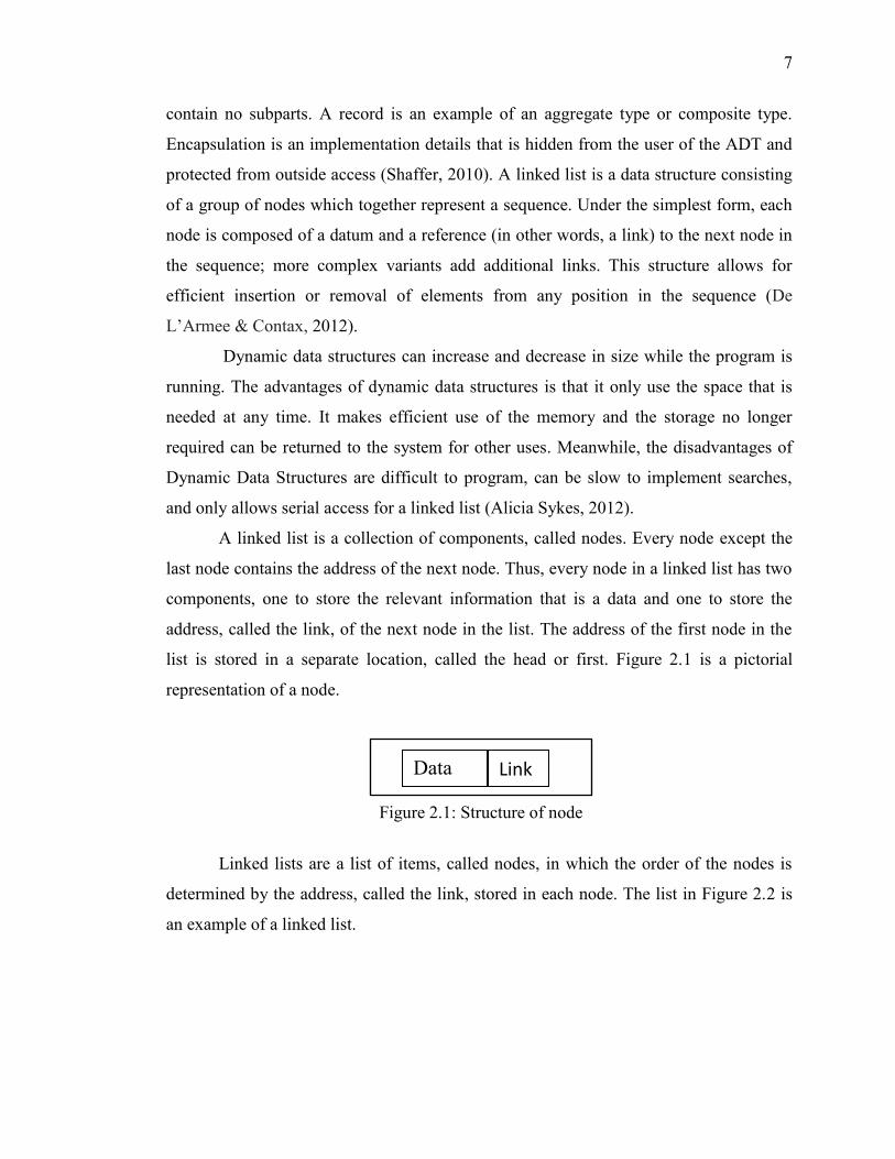
A linked list is a collection of components, called nodes. Every node except the

last node contains the address of the next node. Thus, every node in a linked list has two

components, one to store the relevant information that is a data and one to store the

address, called the link, of the next node in the list. The address of the first node in the

list is stored in a separate location, called the head or first. Figure 2.1 is a pictorial

representation of a node.

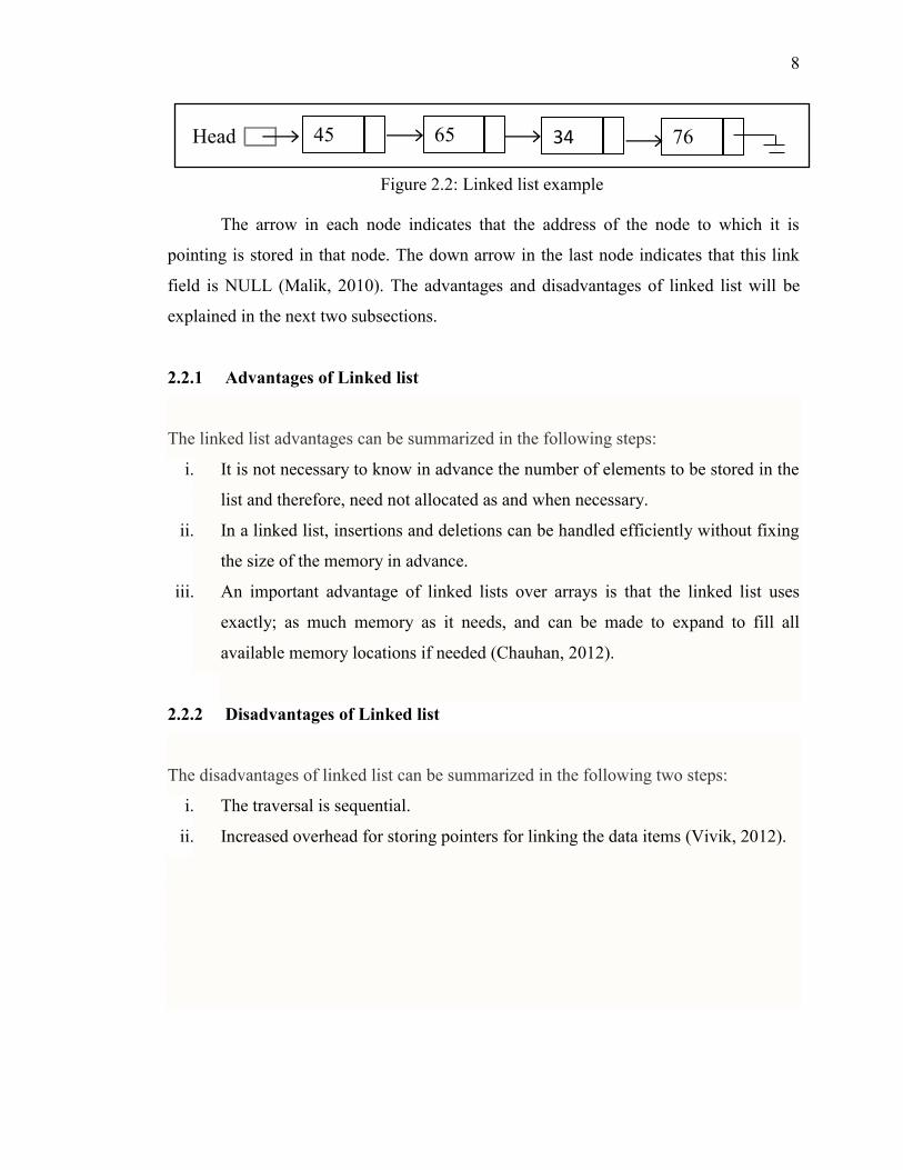
Linked lists are a list of items, called nodes, in which the order of the nodes is

determined by the address, called the link, stored in each node. The list in Figure 2.2 is

an example of a linked list.

Data Link

Figure 2.1: Structure of node

8

The arrow in each node indicates that the address of the node to which it is

pointing is stored in that node. The down arrow in the last node indicates that this link

field is NULL (Malik, 2010). The advantages and disadvantages of linked list will be

explained in the next two subsections.

2.2.1 Advantages of Linked list

The linked list advantages can be summarized in the following steps:

i. It is not necessary to know in advance the number of elements to be stored in the

list and therefore, need not allocated as and when necessary.

ii. In a linked list, insertions and deletions can be handled efficiently without fixing

the size of the memory in advance.

iii. An important advantage of linked lists over arrays is that the linked list uses

exactly; as much memory as it needs, and can be made to expand to fill all

available memory locations if needed (Chauhan, 2012).

2.2.2 Disadvantages of Linked list

The disadvantages of linked list can be summarized in the following two steps:

i. The traversal is sequential.

ii. Increased overhead for storing pointers for linking the data items (Vivik, 2012).

45 76 34 65 Head

Figure 2.2: Linked list example

9

2.3 Sorting Techniques

Sorting means rearranging data in any order, such as ascending; or descending with

numerical data or alphabetically with character data (Dutta, 2013). Sorting is a

commonly used operation in computer science. In addition to its main job, sorting often

require to facilitation of some other operation such as searching, merging and

normalization (Renu & Manisha, 2015). There are many sorting algorithms that are

being used in practical life as well as in computation. A sorting algorithm consists of

comparison, swap, and assignment operations (Khairullah, 2013). The usefulness and

significance of sorting is depicted from day to day application of (Kapur et al., 2012).

Sorting of real life objects, for instance, the telephone directories, incoming tax files,

tables of contents, libraries and dictionaries.

In the following subsection, five sorting algorithms, such as, Bubble Sort,

Insertion Sort, Selection Sort, Merge Sort and Quick Sort will be explained in some of

the details.

2.3.1 Selection Sort

In Selection Sort, a list is sorted by selecting elements in the list, one at a time, and

moving them to their proper positions. This algorithm finds the location of the smallest

element in the unsorted portion of the list and moves it to the top of the unsorted portion

(that is, the whole list) of the list. The first time locates the smallest item in the entire

list; the second locates the smallest item in the list starting from the second element in

the list, and so on. Selection Sort is a sorting algorithm, specifically an in-place

comparison sort. It has an O(n2) complexity, making it inefficient on large lists, and

generally performs worse than the similar Insertion Sort. Selection Sort is noted for its

simplicity and also has performance advantages over more complicated algorithms in

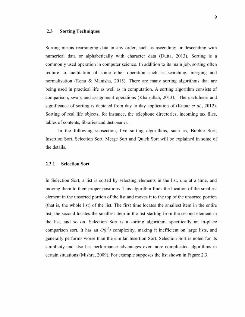
certain situations (Mishra, 2009). For example supposes the list shown in Figure 2.3.

10

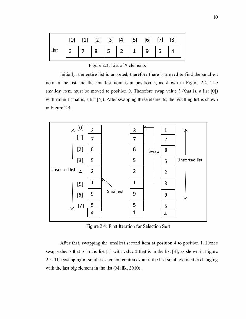
Initially, the entire list is unsorted, therefore there is a need to find the smallest

item in the list and the smallest item is at position 5, as shown in Figure 2.4. The

smallest item must be moved to position 0. Therefore swap value 3 (that is, a list [0])

with value 1 (that is, a list [5]). After swapping these elements, the resulting list is shown

in Figure 2.4.

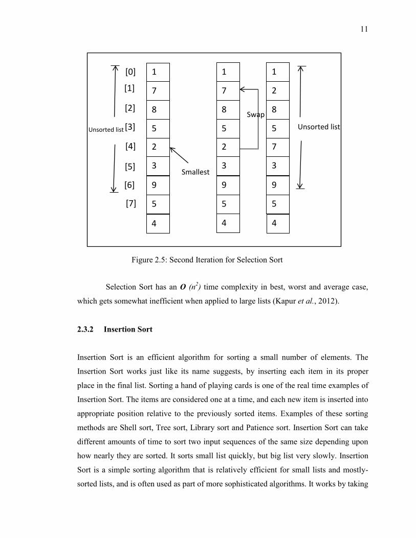
After that, swapping the smallest second item at position 4 to position 1. Hence

swap value 7 that is in the list [1] with value 2 that is in the list [4], as shown in Figure

2.5. The swapping of smallest element continues until the last small element exchanging

with the last big element in the list (Malik, 2010).

7 8

5 2 1 9 5 List

[1] [3] [4] [5] [6] [7] [2]

3

[0]

5

9

1

2

5

8

7

3

5

9

1

2

5

8

7

3

5

9

3

2

5

8

7

1

Unsorted list

Unsorted list

Smallest

Swap

[0]

[1]

[2]

[3]

[4]

[5]

[6]

[7]

4

[8]

4 4 4

Figure 2.3: List of 9 elements

Figure 2.4: First Iteration for Selection Sort

11

Selection Sort has an O (n2) time complexity in best, worst and average case,

which gets somewhat inefficient when applied to large lists (Kapur et al., 2012).

2.3.2 Insertion Sort

Insertion Sort is an efficient algorithm for sorting a small number of elements. The

Insertion Sort works just like its name suggests, by inserting each item in its proper

place in the final list. Sorting a hand of playing cards is one of the real time examples of

Insertion Sort. The items are considered one at a time, and each new item is inserted into

appropriate position relative to the previously sorted items. Examples of these sorting

methods are Shell sort, Tree sort, Library sort and Patience sort. Insertion Sort can take

different amounts of time to sort two input sequences of the same size depending upon

how nearly they are sorted. It sorts small list quickly, but big list very slowly. Insertion

Sort is a simple sorting algorithm that is relatively efficient for small lists and mostly-

sorted lists, and is often used as part of more sophisticated algorithms. It works by taking

[0]

[1]

[2]

[3]

[4]

[5]

[6]

[7] 5

9

3

2

5

8

7

1

Unsorted list

5

9

3

2

5

8

7

1

Swap Unsort

ed list

5

9

3

7

5

8

2

1

Unsorted list

Smallest

4 4 4

Figure 2.5: Second Iteration for Selection Sort

12

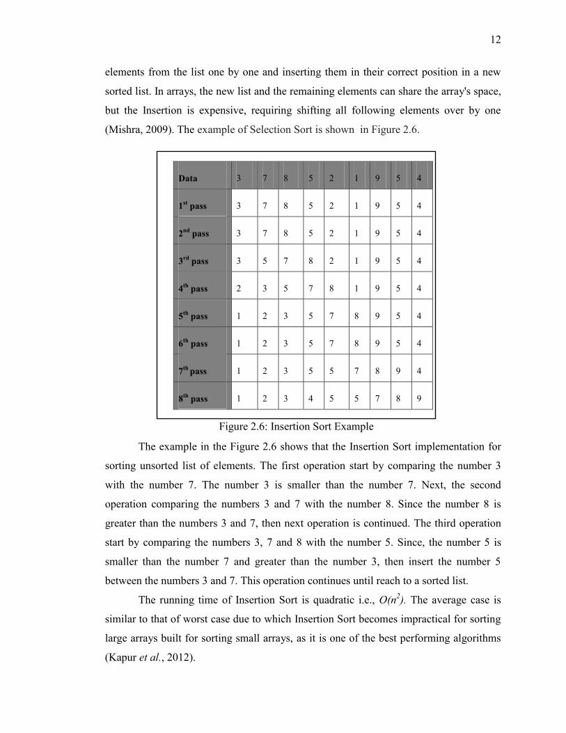
elements from the list one by one and inserting them in their correct position in a new

sorted list. In arrays, the new list and the remaining elements can share the array's space,

but the Insertion is expensive, requiring shifting all following elements over by one

(Mishra, 2009). The example of Selection Sort is shown in Figure 2.6.

Data 3 7 8 5 2 1 9 5 4

1st pass 3 7 8 5 2 1 9 5 4

2nd

pass 3 7 8 5 2 1 9 5 4

3rd

pass 3 5 7 8 2 1 9 5 4

4th

pass 2 3 5 7 8 1 9 5 4

5th

pass 1 2 3 5 7 8 9 5 4

6th

pass 1 2 3 5 7 8 9 5 4

7th

pass 1 2 3 5 5 7 8 9 4

8th

pass 1 2 3 4 5 5 7 8 9

The example in the Figure 2.6 shows that the Insertion Sort implementation for

sorting unsorted list of elements. The first operation start by comparing the number 3

with the number 7. The number 3 is smaller than the number 7. Next, the second

operation comparing the numbers 3 and 7 with the number 8. Since the number 8 is

greater than the numbers 3 and 7, then next operation is continued. The third operation

start by comparing the numbers 3, 7 and 8 with the number 5. Since, the number 5 is

smaller than the number 7 and greater than the number 3, then insert the number 5

between the numbers 3 and 7. This operation continues until reach to a sorted list.

The running time of Insertion Sort is quadratic i.e., O(n2). The average case is

similar to that of worst case due to which Insertion Sort becomes impractical for sorting

large arrays built for sorting small arrays, as it is one of the best performing algorithms

(Kapur et al., 2012).

Figure 2.6: Insertion Sort Example

13

2.3.3 Bubble Sort

Bubble Sort is a basic sorting algorithm that performs the sorting operation by iteratively

comparing the adjacent pair of the given data items and swaps the items if their order is

reversed. There is a repetition of the passes through the list is sorted and no more swaps

are needed. It is a simple algorithm, but it lacks in efficiency when the given input data

set is large. The worst case as well as the average case complexity of Bubble Sort is

О(n2) (Kapur et al., 2012). If have 100 elements, then the total number of comparisons is

10000. Obviously, this algorithm is rarely used except in education (Mishra, 2009).

Bubble Sort is a straightforward and simple method sorting data that is used in computer

science. The algorithm starts at the beginning of the data set. It compares the first two

elements, and if the first is greater than the second, it swaps them. It continues doing this

for each pair of adjacent elements to the end of the data set. It then starts again with the

first two elements, repeating until no swaps have occurred on the last pass (Mishra,

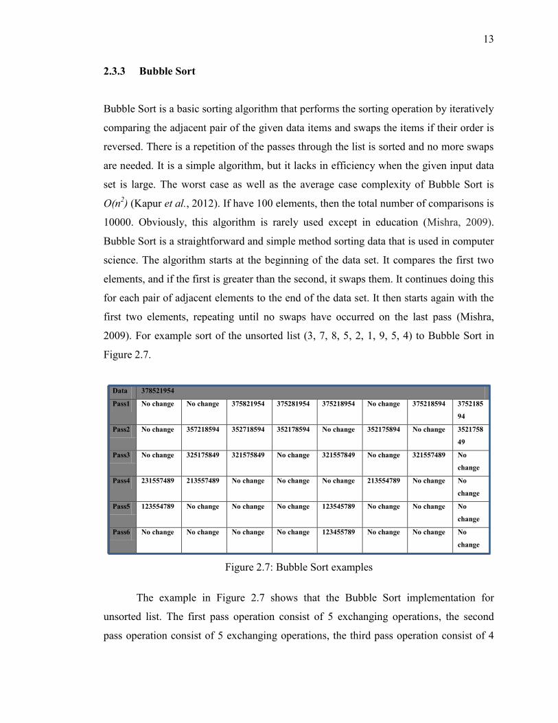
2009). For example sort of the unsorted list (3, 7, 8, 5, 2, 1, 9, 5, 4) to Bubble Sort in

Figure 2.7.

Data 378521954

Pass1 No change No change 375821954 375281954 375218954 No change 375218594 3752185

94

Pass2 No change 357218594 352718594 352178594 No change 352175894 No change 3521758

49

Pass3 No change 325175849 321575849 No change 321557849 No change 321557489 No

change

Pass4 231557489 213557489 No change No change No change 213554789 No change No

change

Pass5 123554789 No change No change No change 123545789 No change No change No

change

Pass6 No change No change No change No change 123455789 No change No change No

change

The example in Figure 2.7 shows that the Bubble Sort implementation for

unsorted list. The first pass operation consist of 5 exchanging operations, the second

pass operation consist of 5 exchanging operations, the third pass operation consist of 4

Figure 2.7: Bubble Sort examples

14

exchanging operations, the fourth pass operation consist of 2 swapping operations and

the fifth pass operation consist of 2 swapping operations. Therefore, the number of

comparison that are used to sort the 9 elements of data in Figure 2.7 is 19 and the

number passes is 5.

2.3.4 Quick Sort

Quick Sort is a very popular sorting algorithm invented by a computer scientist named

C.A.R Hoar back in 1962 (Hoare, 1962). The name comes from the fact that, in general,

Quick Sort can sort a list of data elements significantly faster than any of the common

sorting algorithms. This algorithm is based on the fact that it is faster and easier to sort

two small arrays than one larger one. Quick Sort is based on divide and conquer method.

Quick Sort is also known as partition exchange sort. The Quick Sort operation steps are:

Step 1: One of the elements is selected as the partition element known as pivot element.

Step 2: The remaining items are compared to it and a series of exchanges is performed.

Step 3: When the series of exchanges is done, the original sequence has been partitioned

into three subsequences, all items less than the pivot element, the pivot element in its

final place, all items greater than the pivot element. At this stage, Step 2 is completed

and Quick Sort will be applied recursively to Step 1, and the sequence is sorted when the

recursion terminates (Mishra, 2009).

Quick Sort is a divide and conquer algorithm which relies on a partition

operation, to partition an array, choosing an element; called a pivot, moving all smaller

elements before the pivot, and move all great elements after it. This can be done

efficiently in linear time and in-place. Then the lesser and greater sub lists are

recursively sorted (Mishra, 2009).

With its modest O(log2 n) space usage, this makes Quick sort one of the most

popular sorting algorithms, available in many standard libraries. The more complex

issue in Quick Sort is choosing a good pivot element; consistently poor choices of pivots

can result in drastically slower O(n²) performance, but if at each step the median as the

pivot is chosen then it works in O(nlog2n) (Kapur et al, 2012).

15

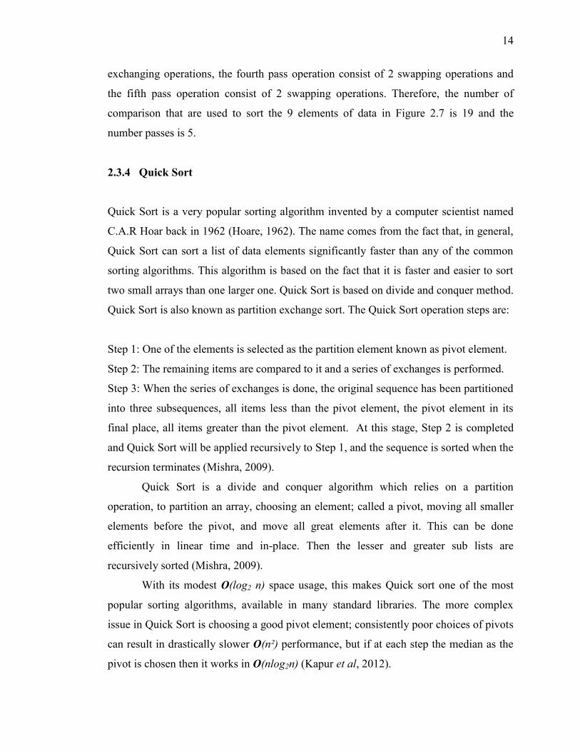
Quick Sort is very efficient when data to be sorted is randomly scattered and it

takes O(nlog2n) time. It does not perform well on nearly sorted data and give time

complexity near to O(n2). Quick Sort's performance is dependent on a pivot (Verma &

Kumar, 2013). The Quick Sort example is shown in Figure 2.8.

Figure 2.8: Quick Sort Examples

In Figure 2.8, the algorithm first selects the random element as a pivot and hides

the pivot meanwhile it reconstructs the array with elements smaller than pivot in the left

sub array. Likewise elements larger than pivot in the right sub array. The algorithm

repeats this operation until the array being sorted. In Figure 2.8 all the pivot elements are

highlighted in circles. It shows that:

16

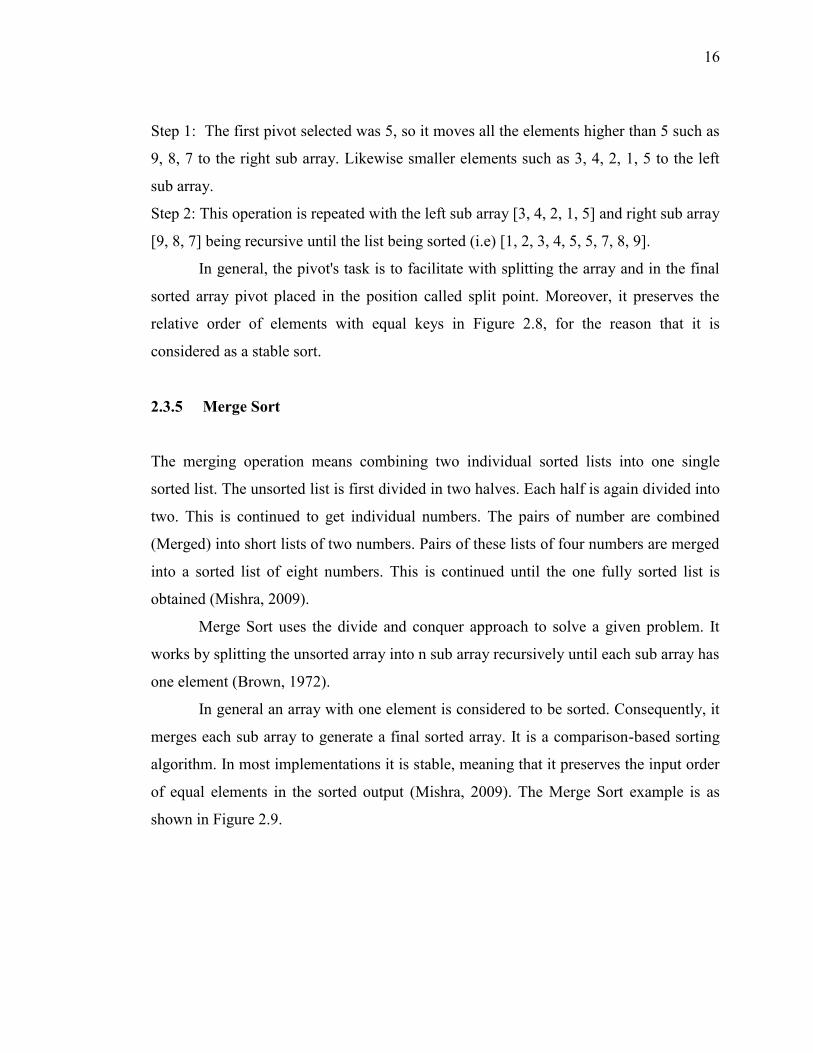
Step 1: The first pivot selected was 5, so it moves all the elements higher than 5 such as

9, 8, 7 to the right sub array. Likewise smaller elements such as 3, 4, 2, 1, 5 to the left

sub array.

Step 2: This operation is repeated with the left sub array [3, 4, 2, 1, 5] and right sub array

[9, 8, 7] being recursive until the list being sorted (i.e) [1, 2, 3, 4, 5, 5, 7, 8, 9].

In general, the pivot's task is to facilitate with splitting the array and in the final

sorted array pivot placed in the position called split point. Moreover, it preserves the

relative order of elements with equal keys in Figure 2.8, for the reason that it is

considered as a stable sort.

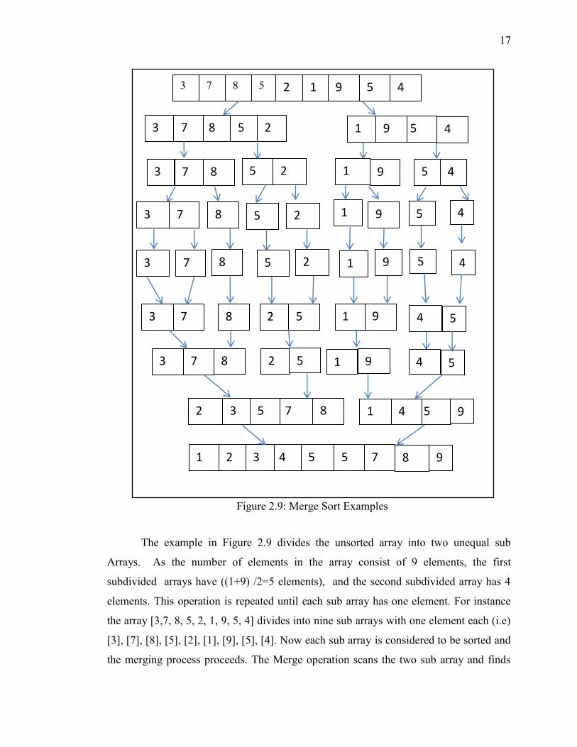
2.3.5 Merge Sort

The merging operation means combining two individual sorted lists into one single

sorted list. The unsorted list is first divided in two halves. Each half is again divided into

two. This is continued to get individual numbers. The pairs of number are combined

(Merged) into short lists of two numbers. Pairs of these lists of four numbers are merged

into a sorted list of eight numbers. This is continued until the one fully sorted list is

obtained (Mishra, 2009).

Merge Sort uses the divide and conquer approach to solve a given problem. It

works by splitting the unsorted array into n sub array recursively until each sub array has

one element (Brown, 1972).

In general an array with one element is considered to be sorted. Consequently, it

merges each sub array to generate a final sorted array. It is a comparison-based sorting

algorithm. In most implementations it is stable, meaning that it preserves the input order

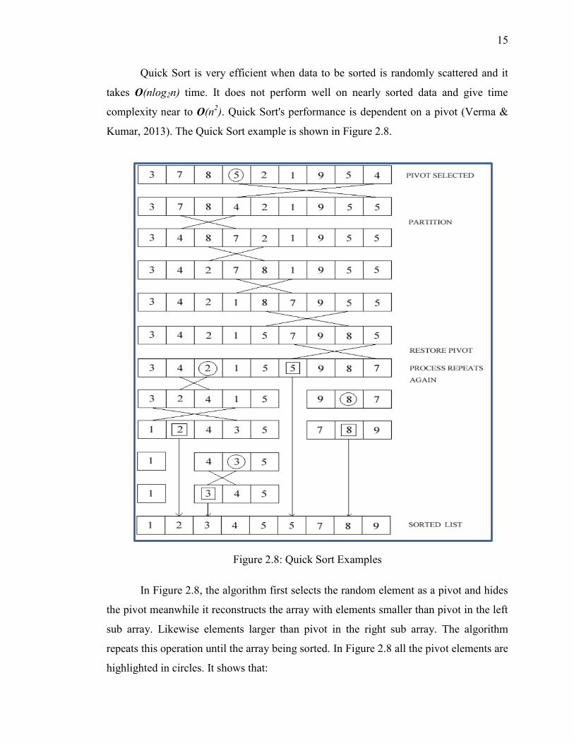
of equal elements in the sorted output (Mishra, 2009). The Merge Sort example is as

shown in Figure 2.9.

17

The example in Figure 2.9 divides the unsorted array into two unequal sub

Arrays. As the number of elements in the array consist of 9 elements, the first

subdivided arrays have ((1+9) /2=5 elements), and the second subdivided array has 4

elements. This operation is repeated until each sub array has one element. For instance

the array [3,7, 8, 5, 2, 1, 9, 5, 4] divides into nine sub arrays with one element each (i.e)

[3], [7], [8], [5], [2], [1], [9], [5], [4]. Now each sub array is considered to be sorted and

the merging process proceeds. The Merge operation scans the two sub array and finds

5 8 3 7 2 1 9 5

5 8 3 7 5 9 2 1

3 7 5 8 2 1 5 9

3 7 8 5 2 1 9 5

3 7 2 8 5 1 4 9

2 3

7 5 8 1 5 4

1 2 4 3 5 5 8 7

4

4

4

4

3 7 8 5 2 1 9 5 4

5

3 7 2 8 1 5 9 4 5

9

9

Figure 2.9: Merge Sort Examples

18

the smallest element thus removes the smallest element and is placed in the final sorted

sub array. This operation is repeated until there is only one sub array left. This sub array

considered to be sorted. For instance the Merge operation takes two sub arrays [3] and

[7], it scans these two arrays and finds that 3 is the smallest element, so it placed 3 in the

first position on the merged sub list and 7 in the second position. This step continues

until only one sub array which is sorted (i.e) [1, 2, 3, 4, 5, 5, 7, 8, 9] (Karunanithi, 2014).

2.4 Time Complexity

The time complexity (Sipser & Michael, 2006) of an algorithm quantifies the amount of

time taken by an algorithm to run as a function of the length of the string representing

the input. The time complexity of an algorithm is commonly expressed using Big-O

Notation, which excludes coefficients and lower order terms. When expressed this way,

the time complexity is said to be described asymptotically, i.e., as the input size goes to

infinity. For example, if the time required by an algorithm on all inputs of size n is at

most 5n3 + 3n for any n, the asymptotic time complexity is O(n

3). The following

subsections are some concepts of the time complexity.

2.4.1 Asymptotic notation

In computer science, generally notations are used to illustrate the asymptotic running

time of algorithms which are defined in terms of functions whose domains are the set of

natural numbers and sometimes real numbers (Cormen et al., 2009).

https://en.wikipedia.org/wiki/Michael_Sipser

https://en.wikipedia.org/wiki/Algorithm

https://en.wikipedia.org/wiki/String_(computer_science)

19

2.4.2 Big-O Notation

The Big-O notation is used to describe tighter upper bound of a function, which states

that the maximum amount of resources needed by an algorithm to complete the

execution (Cormen et al., 2009). Let f(n) and g(n) be functions that map positive integers

to positive real numbers. f (n) is O(g(n)) if there exists a real constant c > 0 and there

exists an integer constant n0 ≥ 1 such that f (n) ≤ c, g (n) for every integer n ≥ n0.

2.4.3 Running Time Analysis

The running time analysis is a theoretical process to categorize the algorithm into a

relative order among function by predicting and calculating approximately the increase

in running time of an algorithm as its input size increases. To ensure the execution time

of an algorithm should anticipate the worst case, average case and best case performance

of an algorithm. These analyses assist the understanding of algorithm complexity

(Karunanithi, 2014).

The worst case time complexity is the criteria that are used to locate the running

time analysis for every sorting technique that are used in this research.

2.4.3.1 Worst Case Analysis

The worst case analysis (Karunanithi, 2014), anticipates the greatest amount of running

time that an algorithm needed to solve a problem for any input of size n. The worst case

running time of an algorithm gives us an upper bound on the computational complexity.

The worst-case complexity of the algorithm is the function defined by the maximum

number of steps taken on any instance of size n. It represents the curve passing through

the highest point of each column. This is shown in Figure 2.10.

20

int x = 0;

for ( int j = 1; j <= n/2; j++ )

for ( int k = 1; k <= n*n; k++ )

x = x + j + k;

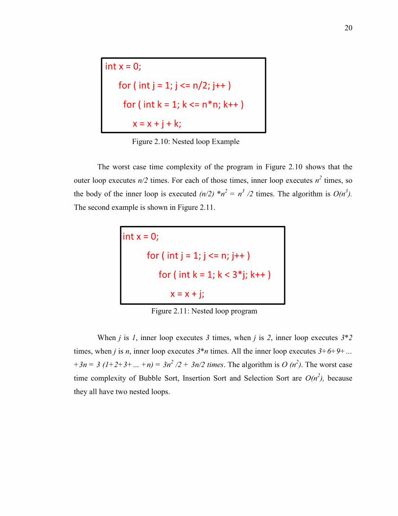
The worst case time complexity of the program in Figure 2.10 shows that the

outer loop executes n/2 times. For each of those times, inner loop executes n2 times, so

the body of the inner loop is executed (n/2) *n2 = n

3 /2 times. The algorithm is O(n

3).

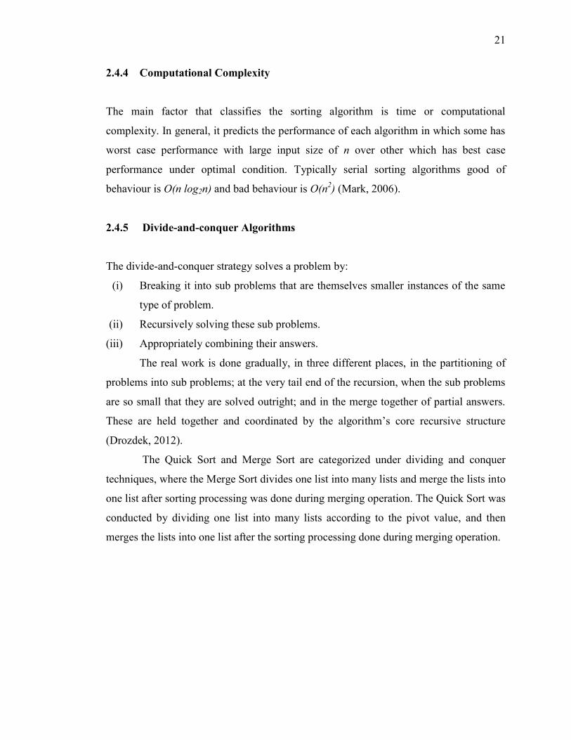
The second example is shown in Figure 2.11.

int x = 0;

for ( int j = 1; j <= n; j++ )

for ( int k = 1; k < 3*j; k++ )

x = x + j;

When j is 1, inner loop executes 3 times, when j is 2, inner loop executes 3*2

times, when j is n, inner loop executes 3*n times. All the inner loop executes 3+6+9+…

+3n = 3 (1+2+3+… +n) = 3n2 /2 + 3n/2 times. The algorithm is O (n

2). The worst case

time complexity of Bubble Sort, Insertion Sort and Selection Sort are O(n2), because

they all have two nested loops.

Figure 2.10: Nested loop Example

Figure 2.11: Nested loop program

21

2.4.4 Computational Complexity

The main factor that classifies the sorting algorithm is time or computational

complexity. In general, it predicts the performance of each algorithm in which some has

worst case performance with large input size of n over other which has best case

performance under optimal condition. Typically serial sorting algorithms good of

behaviour is O(n log2n) and bad behaviour is O(n2) (Mark, 2006).

2.4.5 Divide-and-conquer Algorithms

The divide-and-conquer strategy solves a problem by:

(i) Breaking it into sub problems that are themselves smaller instances of the same

type of problem.

(ii) Recursively solving these sub problems.

(iii) Appropriately combining their answers.

The real work is done gradually, in three different places, in the partitioning of

problems into sub problems; at the very tail end of the recursion, when the sub problems

are so small that they are solved outright; and in the merge together of partial answers.

These are held together and coordinated by the algorithm’s core recursive structure

(Drozdek, 2012).

The Quick Sort and Merge Sort are categorized under dividing and conquer

techniques, where the Merge Sort divides one list into many lists and merge the lists into

one list after sorting processing was done during merging operation. The Quick Sort was

conducted by dividing one list into many lists according to the pivot value, and then

merges the lists into one list after the sorting processing done during merging operation.

22

2.5 Regression

A regression line summarizes the relationship between two variables, but only in a

specific setting, where one of the variables helps explain or predict the other. Regression

describes a relationship between an explanatory variable and a response variable. A

regression line is a straight line that describes how a response variable y changes as an

explanatory variable x changes. Regression line is used to predict the value of y for a

given value of x (Moore, 2010). In the following subsection the linear regression is

explained, which includes the simple linear regression and the estimation least square

regression. This is because the least square regression was used to estimate one value for

each group data elements and execution time for sorting techniques results.

2.5.1 Linear regression

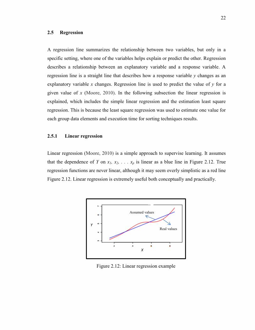
Linear regression (Moore, 2010) is a simple approach to supervise learning. It assumes

that the dependence of Y on x1, x2, . . . xp is linear as a blue line in Figure 2.12. True

regression functions are never linear, although it may seem overly simplistic as a red line

Figure 2.12. Linear regression is extremely useful both conceptually and practically.

Figure 2.12: Linear regression example

Real values

Assumed values

Y

X

23

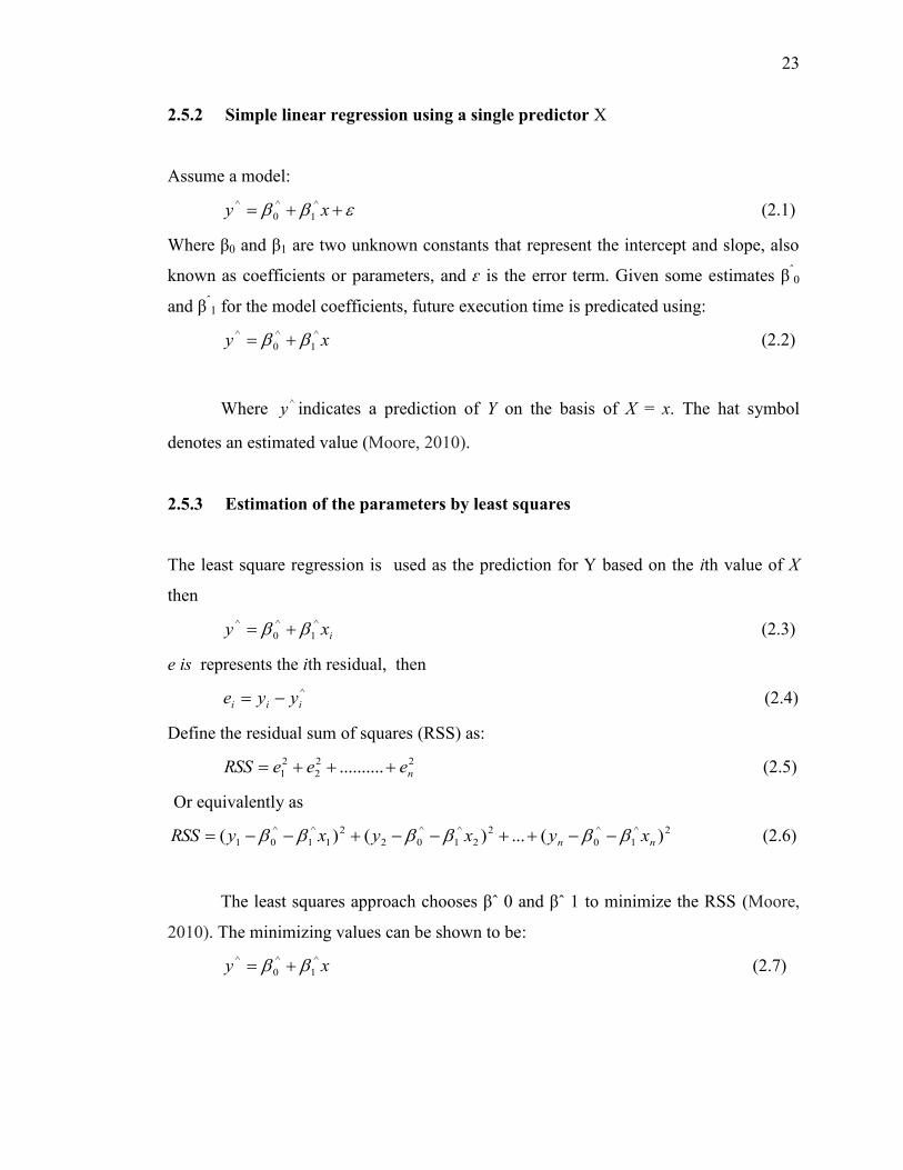
2.5.2 Simple linear regression using a single predictor X

Assume a model:

xy ^

1

^

0

^ (2.1)

Where β0 and β1 are two unknown constants that represent the intercept and slope, also

known as coefficients or parameters, and ԑ is the error term. Given some estimates βˆ0

and βˆ1 for the model coefficients, future execution time is predicated using:

xy ^

1

^

0

^ (2.2)

Where ^y indicates a prediction of Y on the basis of X = x. The hat symbol

denotes an estimated value (Moore, 2010).

2.5.3 Estimation of the parameters by least squares

The least square regression is used as the prediction for Y based on the ith value of X

then

ixy ^

1

^

0

^ (2.3)

e is represents the ith residual, then

^

iii yye (2.4)

Define the residual sum of squares (RSS) as:

22

2

2

1 .......... neeeRSS (2.5)

Or equivalently as

2^

1

^

0

2

2

^

1

^

02

2

1

^

1

^

01 )(...)()( nn xyxyxyRSS (2.6)

The least squares approach chooses βˆ 0 and βˆ 1 to minimize the RSS (Moore,

2010). The minimizing values can be shown to be:

xy ^

1

^

0

^ (2.7)

24

Where:

n

i i

n

i i

xx

yyxx

1

2

1^

1

)(

))(( (2.8)

xy ^

1

^

0 (2.9)

x =

n

i

i

n

x1

(2.10)

n

i

i

n

yy

1 (2.11)

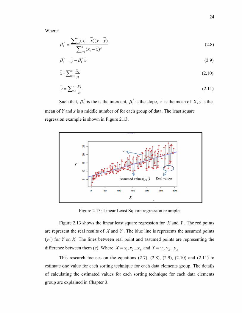
Such that, ^

0 is the is the intercept, ^

1 is the slope, x is the mean of X, y is the

mean of Y and x is a middle number of for each group of data. The least square

regression example is shown in Figure 2.13.

Figure 2.13 shows the linear least square regression for X and Y . The red points

are represent the real results of X and Y . The blue line is represents the assumed points

(yiˆ) for Y on X. The lines between real point and assumed points are representing the

difference between them (e). Where pxxxX ..., 21 and pyyyY ..., 21

This research focuses on the equations (2.7), (2.8), (2.9), (2.10) and (2.11) to

estimate one value for each sorting technique for each data elements group. The details

of calculating the estimated values for each sorting technique for each data elements

group are explained in Chapter 3.

Figure 2.13: Linear Least Square regression example

Real values Assumed values(yiˆ)

ei

Y

X

119

REFERENCES

Alicia Sykes (2012). Data Structure and Manipulation. Retrieved on April 6, 2015, from

http://a2computing.as93.net/downloads/Data%20Structures%20and%20Data%

20Manipulation%20(Everything).pdf.

Aliyu, A. M. and Zirra, P. B. (2013). A Comparative Analysis of Sorting Algorithms

on Integer and Character Arrays. The International Journal of Engineering

and Science. 2(7): 25-30.

Brown, C. (1972). Merge Sort algorithm [M1]. Communications of the ACM. 15(5),

357-358.

Beniwal, S. and Grover, D. (2013). Comparison of various sorting algorithms: A

Review. International Journal of Emerging Research in Management and

Technology. 2(5): 83-86.

Cormen, T. H., Leiserson, C. E., Rivest, R. L. and Stein, C. Introduction to Algorithms.

3rd

Ed. Cambridge: MIT Press. 2009.

De L’Armee, M. and Contax, T. Fundamental Data Structures. International Edition.

Cambridge: Rick Miller. 2012.

Dutta, P. S. (2013). An Approach to Improve the Performance of Insertion Sort

Algorithm. International Journal of Computer Science & Engineering

Technology. 4(5): 503-505.

Drozdek, A. Data Structures and algorithms in C++. 4th

Ed. Thomson Learning:

Brooks/ Cole. 2012.

EL Abbadi, N. K. and Kaeem, Z. Y. A. (2014). NK-Sorting Algorithm. Journal of Kufa

for Mathematics and Computer. 1(4): 27-35.

Horsmalahti, P. (2012). Comparison of Bucket Sort and RADIX Sort. arXiv preprint

arXiv.1(15): 1-10.

Hoare, C. A. (1962). Quicksort. The Computer Journal. 5(1), 10-16

http://a2computing.as93.net/downloads/Data%20Structures%20and%20Data%20Manipulation%20(Everything).pdf

http://a2computing.as93.net/downloads/Data%20Structures%20and%20Data%20Manipulation%20(Everything).pdf

120

Jadoon, S., Solehria, S. F.and Qayum, M. (2011). Optimized Selection Sort Algorithm is

Faster than the Insertion Sort Algorithm: a Comparative Study. International

Journal of Electrical & Computer Sciences.11(02): 19-24,

Jariya Phongsai (2009). Research paper on Sorting Algorithm. Retrieved on May 6,

2015, from http:// www. eportfolio. lagcc. cuny. edu/ scholars/ doc_fa09/

eP_fa09/Jariya.%20Phongsai/documents/mac%20286/sorting%20algorithms%20

research.pdf.

Jain, D. C. (2014). A Comparative Study on Different Types of Sorting Algorithms (On

the Basis of C and Java). International Journal of Computer Science &

Engineering Technology. 5(08): 805-808.

Khairullah, M. (2013). Enhancing Worst Sorting Algorithms. International Journal of

Advanced Science and Technology. 56(1): 13-26.

Karunanithi, A. K. A. Survey Discussion and Comparison of Sorting Algorithms.

Master’s Thesis. Umea˚ University; 2014.

Kapur, Eshan, Kumar, Parveen, Gupta and Sahil (2012). Proposal of a two way sorting

Algorithm and performance Comparison with existing Algorithms.

International Journal of Computer Science, Engineering and Applica. 2(3): 61-

78.

Malik, D. S. Data structures using C++. 2nd

Ed. Course Technology : Cengage

Learning. 2010.

Mishra, A. D. Selection of Best Sorting Algorithm for a Particular problem. Ph.D.

Thesis. Thapar University Patiala; 2009.

Mark A. Weiss. Data Structures Algorithms Analysis in C++. 3rd

Ed. Pearson

Education: Addison-Wesley. 2006.

Moore, D. S. The basic practice of statistics. 5rd

Ed. New Work: W.H. Freeman and

Company. 2010.

Miss. Pooja K. Chhatwani, Miss. Jayashree S. and Somani, (2013). Comparative

Analysis Performance of Different Sorting Algorithm in Data Structure.

Internationa Journal of Advanced Research in Computer Science and Software

Engineering. 3(11): 500-507.

121

Ocampo, J. P. (2008). An empirical comparison of the runtime of five sorting

Algorithms. Retrrived on December 16, 2015, from

http://uploads.julianapena.com/ib-ee.pdf.

Rao, D. D. and Ramesh, B. (2012). Experimental Based Selection of Best Sorting

Algorithm. International Journal of Modern Engineering Research. 2(4),

2908-2912.

Renu and Manisha. (2015). MQ Sort an Innovative Algorithm using Quick Sort and

Merge Sort. International Journal of Computer Applications. 122(21):10-14

Shene, C. K. (1996). A comparative study of linked list sorting algorithms. 3C ON-

LINE, 3(2): 4-9.

Sareen, P. (2013). Comparison of sorting algorithms (on the basis of average

Case). International Journal of Advanced Research in Computer Science and

Software Engineering. 3(3): 522-532.

Swain, D., Ramkrishna, G., Mahapatra, H., Patr, P. and Dhandrao, P. M. A. (2013).

Novel Sorting Technique to Sort Elements in Ascending Order. International

Journal of Engineering and Advanced Technology. 3(1): 212-126.

Sipser and Michael. Introduction to the Theory of Computation. 1st Ed. Thomson:

Course Technology. 2006.

Shaffer, C. A. A Practical Introduction to Data Structures and Algorithm Analysis. 3rd

Ed. Blacksburg: Prentice Hall. 2010.

Vermesan, O., and Friess, P. (Eds.). Internet of things: converging technologies for

smart environments and integrated ecosystems. 1st Ed. Aalborg: River

Publishers. 2013.

Vivek Chauhan, 2012, linked list advantages and disadvantages. Retrieved on

November 4, 2015 from http://solvewithc.blogspot.my/2012/04/linked-list-

advantages-and.html

Verma, A. K., & Kumar, P. (2013). List Sort: A New Approach for Sorting List to

Reduce Execution Time. arXiv preprint arXiv. 1(26): 10-17.

https://en.wikipedia.org/wiki/Michael_Sipser

https://plus.google.com/107569898787794929986

http://solvewithc.blogspot.my/2012/04/linked-list-advantages-and.html

http://solvewithc.blogspot.my/2012/04/linked-list-advantages-and.html

122

Weiss, M. A. Data Structure and problem solving using C++. 2nd

Ed. Addison Wesly:

Pearson. 2003.

Documents

COMPARISON STUDY OF SORTING TECHNIQUES IN DYNAMIC