14 Nuclear Instruments and Methods in Physics Research BI5 (1986) 14-19 North-Holland. Amsterdam

COMPARISON OF THEORETICAL AND EMPIRICAL INTERATOMIC POTENTIALS

D.J. O’CONNOR

Physics Department, University of Newcastle, N.S. W. Australia

J.P. BIERSACK

C-2 Hahn Meitner Insititute Berlin 39, West Germany

Despite a wealth of theoretical and experimental research on interatomic potentials, there has been only limited guidance on how

well each compares to all others. In this report, many popular theoretical potentials are compared to a large range of experimental potentials to gauge the accuracy of the various theoretical models. From this comparison it is found that the “Universal Potential” of Biersack and Ziegler agrees best with the available measurements. Correction factors are derived which give similar agreement for the other potentials, but some systematic deviations still persist at the low or high energy end for most other potentials, as demonstrated

for the Molike potential.

1. Introduction

In all studies of the interaction of energetic particles with solids, the interatomic potential plays a role. In many processes it is the dominant factor in the events which lead to backscattering, sputtering, radiation damage and to the spatial distributions of implanted ions and recoiling atoms. Despite this importance, there is no clear direction on which potential best represents the interaction between energetic particles and so there is little guidance on which should be used in data analysis, theoretical work or computer simulation. The large range of theoretical and experimental determina- tions of the interatomic potential available does nothing more than confuse the issue.

A number of theoretical predictions for the repulsive part of the interaction potential have been made which range from crude estimates to rather detailed calcula- tions. Different models, the inclusion or exclusion of electron exchange and correlation energies, plus other analysis factors have resulted in the differences between these theories being quite large, in some cases orders of magnitude.

Experimental measurements e.g. of scattering cross sections, channeling effects, high temperature diffusion etc. have been used to derive the interatomic potentials by an inversion procedure. While there is an inevitable experimental uncertainty associated with each such de- termination, there is nevertheless sometimes a disagree- ment between similar measurements made by different groups which is in excess of stated errors. As an added complication to the choice of a potential and the ap- propriate potential parameters, most experimental de- terminations involve inert gas and alkali atoms or ions.

As a result such potentials are of little use in ion solid interactions because although such species are often used as the bombarding particle, they rarely make up the target material.

To reconcile these differences it is necessary to make comparisons between the popular theoretical potentials and an extensive range of empirical potentials. Such a comparison has previously been applied to the Molikre potential [1,2], but now this work has been extended to cover all currently popular forms of the interatomic

potential.

In a previous study [l] of the Moli&e potential it was found that a better agreement between the empirical potentials and the Molikre one could be obtained if a correction factor of the form

f= o.o45(JzT+ 6) +0.54

was applied to the screening length. In subsequent work [2] a more detailed analysis investigated systematic de- partures form this fitting procedure. To emphasise these departures the empirical potentials were divided into two groups depending on whether they represented the potential above, or below, 10 eV. When the same fitting procedure was followed it was found that the correction factor was different for each case as shown below.

V>lOeV f, =l.O*O.l.

V<lOeV f,=O.O485(fi+Jz,)+O.51.

The evident difference between these two cases leads to the conclusion that the form of the Molikre screening function does not properly describe the true screening function over the whole range and thus a better screen- ing function should be sought. The results of this ex- tended analysis are described below.

0168-583X/86/$03.50 0 Elsevier Science Publishers B.V. (North-Holland Physics Publishing Division)

D.J. O’Connor, J. P. Blersd ,j Con~purr.wn of ~~~terutorm potentids 15

2. Theoretical considerations and potentials scattering angle and/or the transferred energy. In this case it is practical to use a repulsive potential written in

In atomic collision problems, the classical collision the form integral has to be evaluated in order to determine the

0 IO

-1 lo

-2 10

I -3

10

-4 IO

-5 10

UNIVERSAL a q,,= L,8 u&s 0.08

LEN2 JENSEN C

o:,, i 142

a&$: 0.20

SOMMERFELO

-1 IO

-2 10

# -3

la

-4 10

-5 10

0 10

Kr-C b

10 5

-1 10

-2 10

& -3

10

-4 10

-5 10

MOLIERE d u;,, i 231

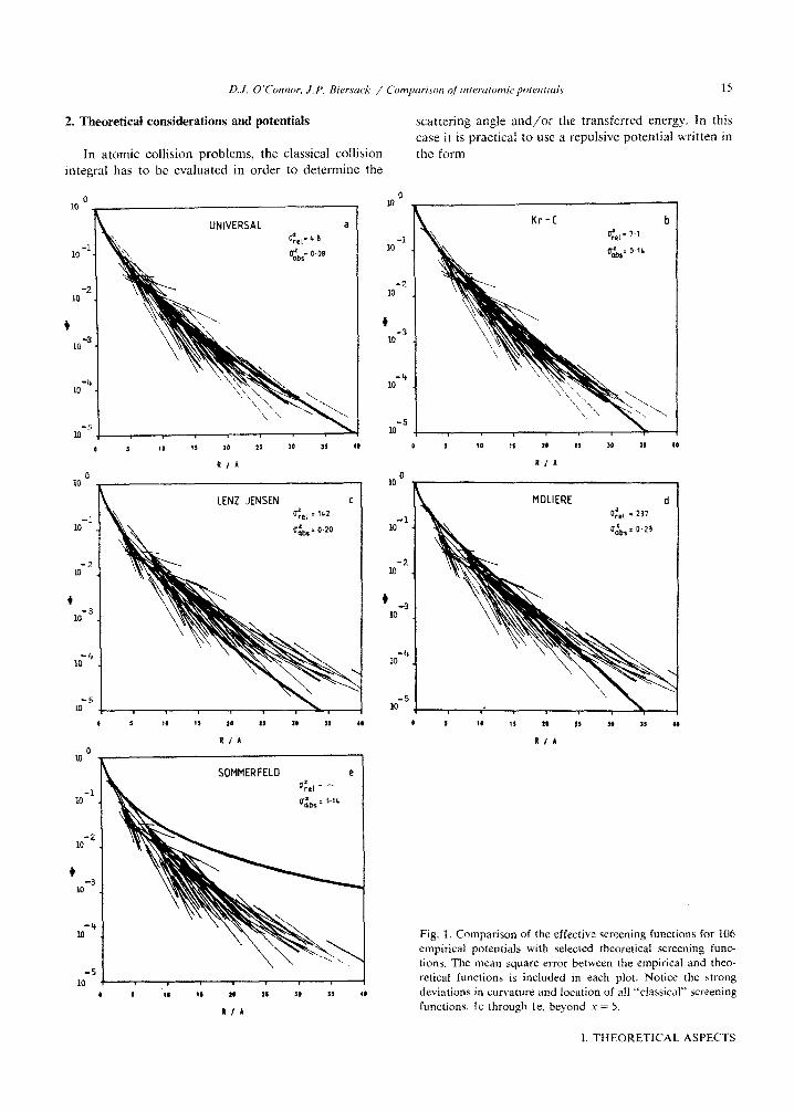
Fig. 1. Comparison of the effective screening functions for 106 empirical potentials with selected theoretical screening func- tions. The mean square error between the empirical and theo-

retical functions is included in each plot. Notice the strong

deviations in curvature and location of all “classical” screening

functions. lc through le, beyond x = S.

I. THEORETICAL ASPECTS

16

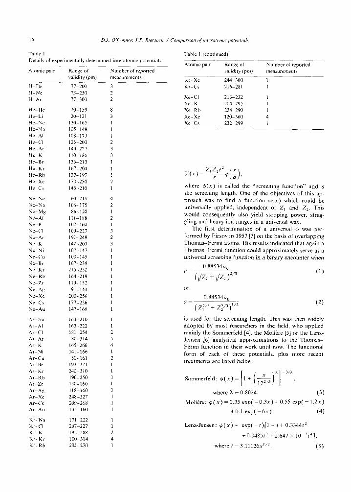
Table 1

Details of experimentally determined interatomic potentials

Atomic pair Range of Number of reported

Table 1 (continued)

Atomic pair Range of

validity (pm)

Number of reported

measurements

validity (pm) measurements Kr-Xe 244-300 1

H-He 77-200

H-Ne 73-250

H-Ar 77-300

He-He 20-159

He-Li 20-121

He-Ne 130-165

He-Na 105-149

He-Al 108-173

He-Cl 125-200

He-Ar 140-227

He-K 110-186

He-Br 136-213

He-Kr 167-204

He-Rb 137-197

He-Xe 173-250

He-C’s 145-210

Ne-Ne 60-218

Ne-Na 10x-175

Ne-Mg X6-120

Ne-AI Ill-188

Ne-P 102-160

Ne-Cl loo-227

Ne-Ar 191-249

Ne-K 142-207

Ne-Ni 107-147

Ne-Cu 100-145

Ne-Br 167-239

Ne-Kr 215-252

Ne-Rb 164-219

Ne-Zr 110-152

Ne-Ag 91-141

Ne-Xe 200-256

Ne-Cs 177-236

Ne-Au 147-169

Ar-Na 163-210

Ar-AI 163-222

Ar-Cl 181-254

Ar-Ar 80-314

Ar-K 165-266

Ar-Ni 141-166

Ar-Cu 50-161

Ar-Br 193-271

Ar-Kr 240-310

Ar-Rb 190-250

Ar-Zr 130-160

Ar-Ag 118-160

Ar-Xe 248-327

Ar-Cs 209-268

Ar-Au 135-160

Kr-Na 171-222

Kr-Cl 207-227

Kr-K 192-288

Kr-Kr 100-314

Kr-Rb 205-270

Kr-Cs 216-281 1

Xe-Cl 213-232 1

Xe-K 204-295 1

XeeRb 224-290 1 XeeXe 120-360 4 Xe-Cs 232-299 1

1

2

4

2 1 2 1

3 2 3 1

1

1

1

1

1

1

where 4(x) is called the “screening function” and a the screening length. One of the objectives of this ap- proach was to find a function +(x) which could be universally applied, independent of Z, and Z,. This would consequently also yield stopping power, strag- gling and heavy ion ranges in a universal way.

The first determination of a universal $I was per- formed by Firsov in 1957 [3] on the basis of overlapping Thomas-Fermi atoms. His results indicated that again a Thomas-Fermi function could approximately serve as a universal screening function in a binary encounter when

0.88534a, (1)

or

0.88534~ a=

( 273 + z;/3y

(2)

is used for the screening length. This was then widely adopted by most researchers in the field, who applied mainly the Sommerfeld [4], the Moliere [5] or the Lenz- Jensen [6] analytical approximations to the Thomas- Fermi function in their work until now. The functional

form of each of these potentials, plus more recent treatments are listed below.

Sommerfeld: +(.x)= [I + [-&iA]13”.

where X = 0.8034. (3)

Moliere: +(,x) = 0.35 exp( -0.3x) + 0.55 exp( - 1.2x)

+O.l exp( -6x). (4)

Lenz-Jensen: +(,Y) = exp( -r)[l + t + 0.33441’

+O.O485t’+ 2.647 x 10V7r4].

where I = 3.11126.x”‘. (5)

D.J. O’Connor, J. P. Biersuck / Comparison o/interotomicpotentiul:, 17

Krypton-carbon [ 71:

+(x) = 0.190945 exp( -0.278544~)

+ 0.473674 exp( -0.637174.x)

-to.335381 exp( - 1.919249x). (6)

I!niversal [ 81:

+(x)=0.1818 exp(-3.2x)+0.5099 exp(-0.9423x)

+0.2802 exp( -0.4029x) + 0.02817

xexp(-0.2016.x). (7)

Last of these (the “Universal” potential) is actually I he one chose for calculating the low energy nuclear

stopping, straggling and projected range moments in the rxhaustive monograph on stopping and ranges edited by Ziegler [42], because its derivation includes exchange and correlation energies and it appeared to give im- proved agreement with the experimental range data.

The dimensionless length x, in the atomic separation I devided by the screening length u. For the Kr-C and I he universal screening functions a new screening length

1 as been derived [8], and is given by

0.88534~~ (8)

3. Comparison with experimentally determined potentials

For this comparison more than a hundred inter- atomic potentials [9-411, derived mainly from scattering experiments, have been collected from the literature. A list of the combinations is compiled in table 1 together with their range of validity. It should be noticed that the presently available data are heavily dominated by rare gases and alkali metals, and not really representative of a statistical average over the entire periodic table.

The use of the effective experimental screening func-

tlon, defined as

V(r)r 0 =- exp Z,Z2e2

allows the comparison between the empirical potentials [9-411, and the theoretical potentials. Such a compari- son is made in fig. 1 for each of the listed theoretical potentials. A visual inspection reveals that the shape of the new “universal” potential has the correct curvature and by virtue of the chosen screening length, eq. (8), is also located in the centre of the experimental data. The Kr-C potential and, more so, the Moliere potential have too little curvature (the Moliere potential is practi- cally a straight line between x = 5 and x = 35). The Lenz-Jensen and Sommerfeld curves respectively, are located below and above the experimental data.

If one inspects more closely the bunching of experi- mental data (disregarding for the moment any theoreti-

cal curve), one may find the experimental lines more

closely grouped together is the upper figures which use the new screening length of eq. (8). The widest scatter is

seen to occur in the last figure using the screening length of eq. (2). Of course, some scatter will always remain, due in part to realistic individual deviations, and due in part to experimental uncertainties associated with each such measurement.

The quality of fit of the empirical curves to each theoretical screening function can be determined as the mean square error in two ways: (1) By the standard

method of calculating the average of the rduttue errors squared, i.e. or’,, = (l/n ) C:,=, AZ with

A’, = d.u

x2 - Xl

where each experiment is given the same weight, inde- pendent of the covered range x2 - x,. (2) By calculating the average of the squares of the obso/ute deviations on a logarirhmic scale, i.e. u,& = (l/n)Ey= ,S,’ with

which corresponds to the visual impression when ob- serving the distances between experiment and theory on

a logarithmic graphical display. The second method for the error determination is not quite standard, but was chosen for two good reasons: (i) for small deviations both methods yield identical results (which may be verified easily by the reader), and (ii) for large devia- tions, e.g. with the Thomas-Fermi potential, our second method is superior as it is symmetric in $I_ and $I~,,, while the standard method depends strongly on the choice of reference, as

(11) For each theoretical potential the mean square error was calculated according to eqs. (9) and (lo), and listed in the third column of tables 2 and 3. respectively.

The empirical potentials were then fitted to each of the theoretical potentials in turn by the introduction of a correction factor to the screening length which mini- mised the error between the empirical potentials and the theoretical potential. The existence, in most cases, of a systematic behaviour between these correction factors and the atomic numbers Z, and Z, has allowed the correction factors to be expressed in the form

acorr =/a (12)

with

r=a(fi+@Y)+P, (13)

where (Y and p are listed in tables 2 and 3. The use of these correction factors to the screening lengths ulti- mately resulted in greatly improved mean square errors for some theoretical potentials, see last column of tables

I. THEORETICAL ASPECTS

18 D.J. O’Connor, J. P. Biersuck / Comporrson of mrerutomic poten~ruls

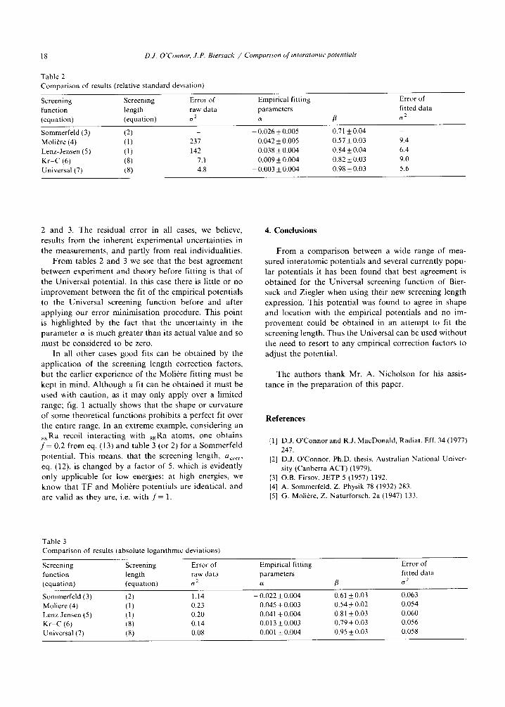
Table 2 Comparison of results (relative standard deviation)

Screening Screening Error of

function length raw data (equation) (equation) (Yz

Sommerfeld (3) (2) _ Moliere (4) (1) 237

Lenz-Jensen (5) 0) 142 Kr-C (6) (8) 7.1

Universal (7) (8) 4.8

Empirical fitting

parameters 11

- 0.026 + 0.005 0.042 f 0.005

0.038 k 0.004

0.009 * 0.004

- 0.003 * 0.004

Error of

fitted data

B 02

0.71 * 0.04 0.57 * 0.03 9.4

0.84 f 0.04 6.4 0.82 i 0.03 9.0

0.98 k 0.03 5.6

2 and 3. The residual error in all cases, we believe, results from the inherent experimental uncertainties in the measurements, and partly from real individualities.

From tables 2 and 3 we see that the best agreement between experiment and theory before fitting is that of the Universal potential. In this case there is little or no improvement between the fit of the empirical potentials to the Universal screening function before and after applying our error minimisation procedure. This point is highlighted by the fact that the uncertainty in the parameter a is much greater than its actual value and so must be considered to be zero.

In all other cases good fits can be obtained by the application of the screening length correction factors, but the earlier experience of the Moliere fitting must be kept in mind. Although a fit can be obtained it must be used with caution, as it may only apply over a limited range; fig. 1 actually shows that the shape or curvature of some theoretical functions prohibits a perfect fit over the entire range. In an extreme example, considering an sxRa recoil interacting with xxRa atoms, one obtains f= 0.2 from eq. (13) and table 3 (or 2) for a Sommerfeld potential. This means, that the screening length, ucorr, eq. (12). is changed by a factor of 5, which is evidently only applicable for low energies; at high energies, we know that TF and Moliere potentials are identical, and

are valid as they are, i.e. with f= 1.

Table 3

Comparison of results (absolute logarithmic deviations)

4. Conclusions

From a comparison between a wide range of mea- sured interatomic potentials and several currently popu- lar potentials it has been found that best agreement is obtained for the Universal screening function of Bier- sack and Ziegler when using their new screening length expression. This potential was found to agree in shape and location with the empirical potentials and no im- provement could be obtained in an attempt to fit the screening length. Thus the Universal can be used without the need to resort to any empirical correction factors to adjust the potential.

The authors thank Mr. A. Nicholson for his assis-

tance in the preparation of this paper.

References

[l] D.J. O’Connor and R.J. MacDonald, Radial. Eff. 34 (1977)

247.

[2] D.J. O’Connor, Ph.D. thesis, Australian National Univer-

sity (Canberra ACT) (1979).

[3] O.B. Firsov, JETP 5 (1957) 1192. [4] A. Sommerfeld, Z. Physik 78 (1932) 283.

[5] G. Moliere, Z. Naturforsch. 2a (1947) 133.

Screening

function

(equation)

Screening

length

(equation)

Sommerfeld (3)

Moliere (4) Lenz Jensen (5)

Kr-C (6)

Universal (7)

(2) 1.14

(1) 0.23

(1) 0.20

(8) 0.14

(8) 0.08

Error of Empirical fitting

raw data parameters

az (Y P

- 0.022 * 0.004 0.61 + 0.03 0.063 0.045 * 0.003 0.54 + 0.02 0.054 0.041 * 0.004 0.81 k 0.03 0.060 0.013 + 0.003 0.79 & 0.03 0.056

0.001 * 0.004 0.95 * 0.03 0.058

Error of

fitted data

(Yz

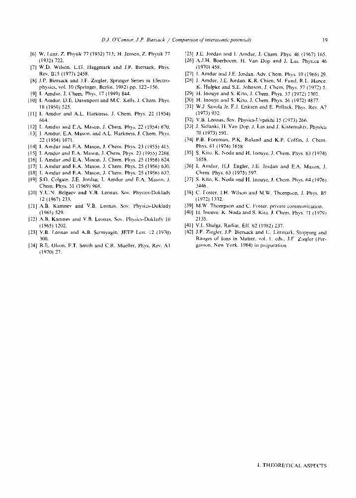
D.J. O’Connor, J.P. Bwrscrck / Comparrson ojinterotomr~potentrals 19

[6] W. Lenz. Z. Physik 77 (1932) 713; H. Jensen, 2. Physik 77

(1932) 722.

[7] W.D. Wilson, L.C. Haggmark and J.P. Biersack. Phys.

Rev. B15 (1977) 2458.

[8] J.P. Biersack and J.F. Ziegler, Sprmger Series in Electro-

physics. vol. 10 (Springer. Berlin. 1982) pp. 122-156.

[9] 1. Amdur, J. Chem. Phys. 17 (1949) 844.

1 IO] I. Amdur. D.E. Davenport and M.C. Kells, J. Chem. Phys.

18 (1950) 525.

Ill] I. Amdur and A.L. Harkness, J. Chem. Phys. 22 (1954)

664.

1121 I. Amdur and E.A. Mason. J. Chem. Phys. 22 (1954) 670.

1131 I. Amdur, E.A. Mason. and A.L. Harkness. J. Chem. Phys.

22 (1954) 1071.

1141 I. Amdur and E.A. Mason, J. Chem. Phys. 23 (1955) 415.

1151 I. Amdur and E.A. Mason, J. Chem. Phys. 23 (1955) 2268.

1161 I. Amdur and E.A. Mason. J. Chem. Phys. 25 (1956) 624.

1171 I. Amdur and E.A. Mason. J. Chem. Phys. 25 (1956) 630.

1181 I. Amdur and E.A. Mason, J. Chem. Phya. 25 (1956) 632.

1191 SO. Colgate. J.E. Jordan. 1. Amdur and E.A. Mason, J.

Chem. Phys. 51 (1969) 968.

1201 Y.U.N. Belgaev and V.B. Leonas. Sov. Physics-Doklady

12 (1967) 233.

1211 A.B. Kamnev and V.B. Leonas. Sov. Physics-Doklady

(1965) 529.

122) A.B. Kamnev and V.B. Leonas. Sov. Physics-Doklady 10

(1965) 1202.

1231 V.B. Leonas and A.B. Sermyagin, JETP Lett. 12 (1970) 300.

1241 R.E. Olson, F.T. Smith and C.R. Mueller. Phys. Rev. Al

(1970) 27.

[25] J.E. Jordan and I. Amdur, J. Chem. Phys. 46 (1967) 165.

[26] A.J.H. Boerboom. H. Van Dop and J. Las. Physica 46

(1970) 458.

[27] I. Amdur and J.E. Jordan, Adv. Chem. Phys. 10 (1966) 29.

[28] 1. Amdur, J.E. Jordan. K.R. Chien. M. Fund. R.L. Hance.

K. Hulpke and S.E. Johnson. J. Chem. Phys. 57 (1972) 5.

[29] H. Inouye and S. Kito, J. Chem. Phys. 57 (1972) 1301.

[30] H. Inouye and S. Kito. J. Chem. Phys. 56 (1972) 4877.

[31] W.J. Savola Jr, F.J. Eriksen and E. Pollack. Phys. Rev. A7

(1973) 932.

[32] V.B. Leonas. Sov. Physics-Uspekhi 15 (1973) 266.

[33] J. Sielanki, H. Van Dop. J. Las and J. Kistemaker. Physica

70 (1973) 591.

(341 P.B. Foreman, P.K. Roland and K.P. Coffin, J. Chem.

Phys. 61 (1974) 1658.

[35] S. Kito. K. Noda and H. Inouye. J. Chem. Phys. 63 (1974)

1658.

[36] 1. Amdur, H.J. Engler. J.E. Jordan and E.A. Mason. J.

Chem. Phys. 63 (1975) 597.

[37] S. Kite, K. Noda and H. Inouye, J. Chem. Phys. 64 (1976)

3446.

[38] C. Foster, I.H. Wilson and M.W. Thompson. J. Phys. BS

(1972) 1332.

[39] M.W. Thompson and C. Foster. private communication.

(401 H. Inouye, K. Noda and S. Kita. J. Chem. Phys. 71 (1979)

2135.

[41] V.I. Shulga. Radiat. Eff. 62 (1982) 237.

[42] J.F. Ziegler, J.P. Biersack and U. Littmark. Stopping and

Ranges of Ions in Matter. vol. 1. eds.. J.F. Ziegler (Per-

gamon. New York. 1984) in preparation.

I. THEORETICAL ASPECTS