Embed Size (px)
Citation preview
Comparison of Seston Composition and Sources in the Delta during two High-flow Falls (2006 and 2011)
Carol Kendall
U.S. Department of the InteriorU.S. Geological Survey
Steve Silva, Megan Young, Jen Lehman (USGS)
Marianne Guerin (RMA)
Slightly updated (mainly to remove overlapping animation graphics) from the presentation on July 31, 2012 in Sacramento, CA

1000
2000
3000
4000
5000
6000
7000
8000
9000
Water Year1970 2010200019901980
Hab
itat I
ndex
Wet
Ab. Normal
Bl. Normal
Dry
Crit. Dry
200920102011
(modified from Feyrer et al. 2010)
2006
The X2-habitat curve approach only explains about 25% of the variance in smelt presence-absence, despite the strong
long-term association between smelt occurrence and salinity and turbidity (Feyrer et al. 2010).
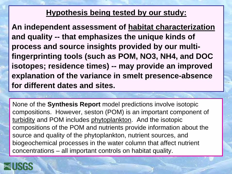
Hypothesis being tested by our study:
An independent assessment of habitat characterization and quality -- that emphasizes the unique kinds of process and source insights provided by our multi- fingerprinting tools (such as POM, NO3, NH4, and DOC isotopes; residence times) -- may provide an improved explanation of the variance in smelt presence-absence for different dates and sites.
None of the Synthesis Report model predictions involve isotopic compositions. However, seston (POM) is an important component of turbidity and POM includes phytoplankton. And the isotopic compositions of the POM and nutrients provide information about the source and quality of the phytoplankton, nutrient sources, and biogeochemical processes in the water column that affect nutrient concentrations – all important controls on habitat quality.
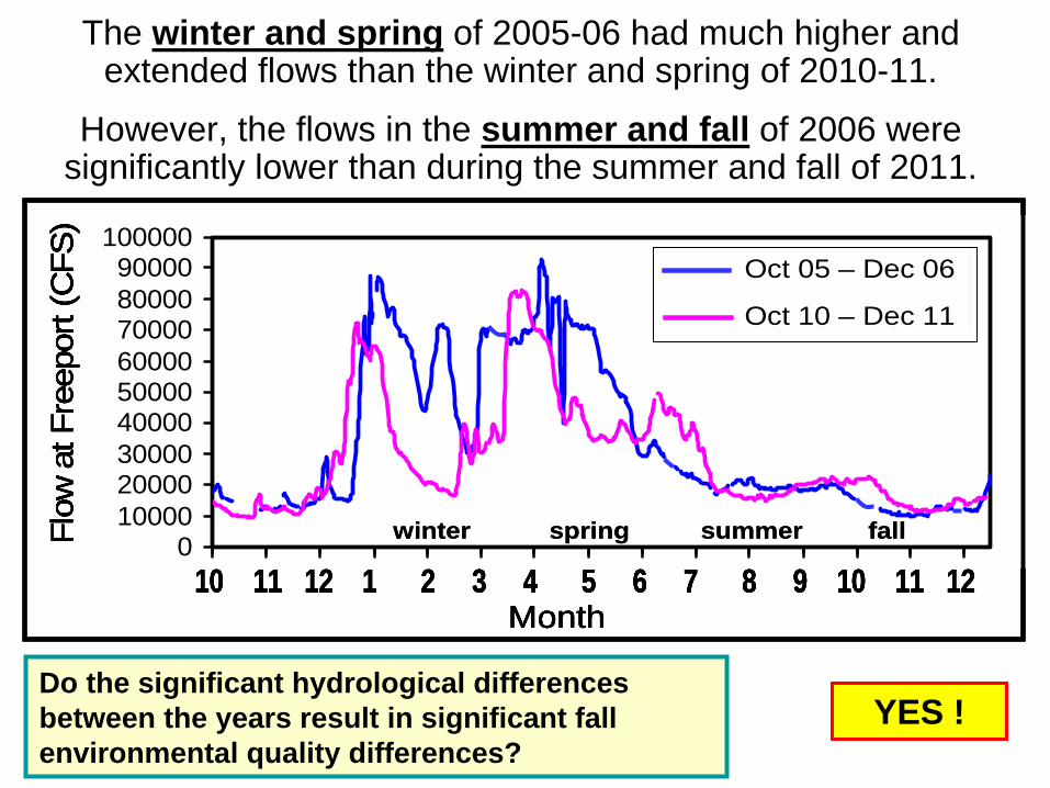
The winter and spring of 2005-06 had much higher and extended flows than the winter and spring of 2010-11.
However, the flows in the summer and fall of 2006 were significantly lower than during the summer and fall of 2011.
0100002000030000400005000060000700008000090000
10000020062011
10 11 12 1 2 3 4 5 6 7 8 9 10 11 12
Flow
at F
reep
ort (
CFS
)
Month
Oct 05 – Dec 06
Oct 10 – Dec 11
winter spring summer fall0100002000030000400005000060000700008000090000
10000020062011
10 11 12 1 2 3 4 5 6 7 8 9 10 11 12
Flow
at F
reep
ort (
CFS
)
Month
Oct 05 – Dec 06
Oct 10 – Dec 11
0100002000030000400005000060000700008000090000
10000020062011
10 11 12 1 2 3 4 5 6 7 8 9 10 11 12
Flow
at F
reep
ort (
CFS
)
Month
Oct 05 – Dec 06
Oct 10 – Dec 11
0100002000030000400005000060000700008000090000
10000020062011
10 11 12 1 2 3 4 5 6 7 8 9 10 11 12
Flow
at F
reep
ort (
CFS
)
Month
Oct 05 – Dec 06
Oct 10 – Dec 11
0100002000030000400005000060000700008000090000
10000020062011
10 11 12 1 2 3 4 5 6 7 8 9 10 11 12
Flow
at F
reep
ort (
CFS
)
Month
Oct 05 – Dec 06
Oct 10 – Dec 11
Oct 05 – Dec 06
Oct 10 – Dec 11
winter spring summer fallwinter spring summer fall
Do the significant hydrological differences between the years result in significant fall environmental quality differences?
YES !
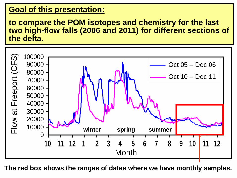
The red box shows the ranges of dates where we have monthly samples.
0100002000030000400005000060000700008000090000
10000020062011
10 11 12 1 2 3 4 5 6 7 8 9 10 11 12
Flow
at F
reep
ort (
CFS
)
Month
Oct 05 – Dec 06
Oct 10 – Dec 11
winter spring summer
Goal of this presentation:to compare the POM isotopes and chemistry for the last two high-flow falls (2006 and 2011) for different sections of the delta.
++
RV Polaris sitesSlough study sites
Sacramento River
San Joaquin River
Suisun
Confluence
Cache
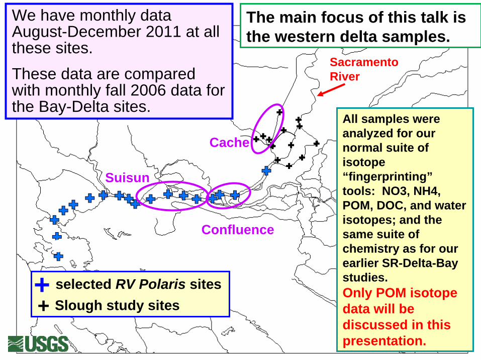
We have monthly data August-December 2011 at all these sites. These data are compared with monthly fall 2006 data for the Bay-Delta sites.
++
selected RV Polaris sitesSlough study sites
++
selected RV Polaris sitesSlough study sites
All samples were analyzed for our normal suite of isotope “fingerprinting” tools: NO3, NH4, POM, DOC, and water isotopes; and the same suite of chemistry as for our earlier SR-Delta-Bay studies. Only POM isotope data will be discussed in this presentation.
The main focus of this talk is the western delta samples.
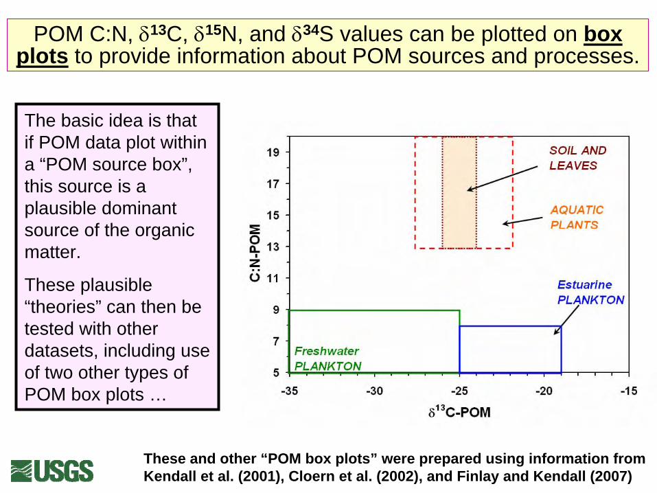
POM C:N, δ13C, δ15N, and δ34S values can be plotted on box plots to provide information about POM sources and processes.
The basic idea is that if POM data plot within a “POM source box”, this source is a plausible dominant source of the organic matter.
These plausible “theories” can then be tested with other datasets, including use of two other types of POM box plots …
These and other “POM box plots” were prepared using information from Kendall et al. (2001), Cloern et al. (2002), and Finlay and Kendall (2007)
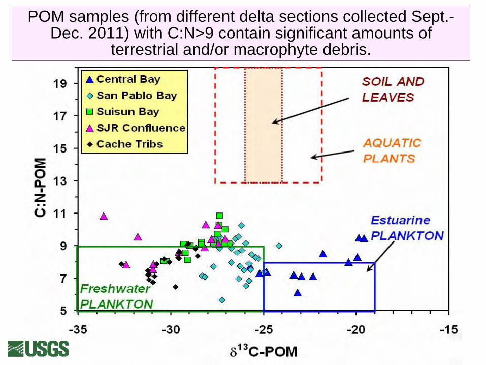
POM samples (from different delta sections collected Sept.- Dec. 2011) with C:N>9 contain significant amounts of
terrestrial and/or macrophyte debris.
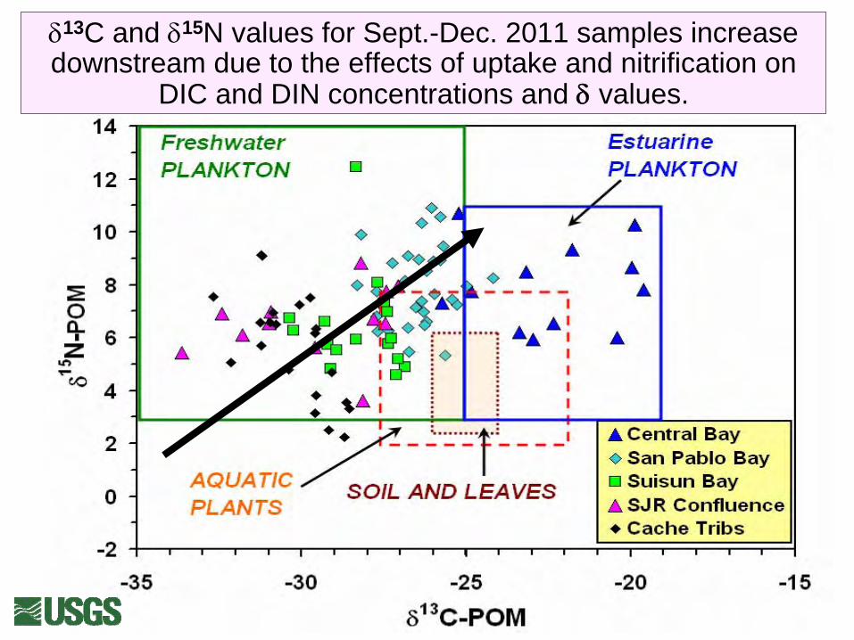
δ13C and δ15N values for Sept.-Dec. 2011 samples increase downstream due to the effects of uptake and nitrification on
DIC and DIN concentrations and δ
values.
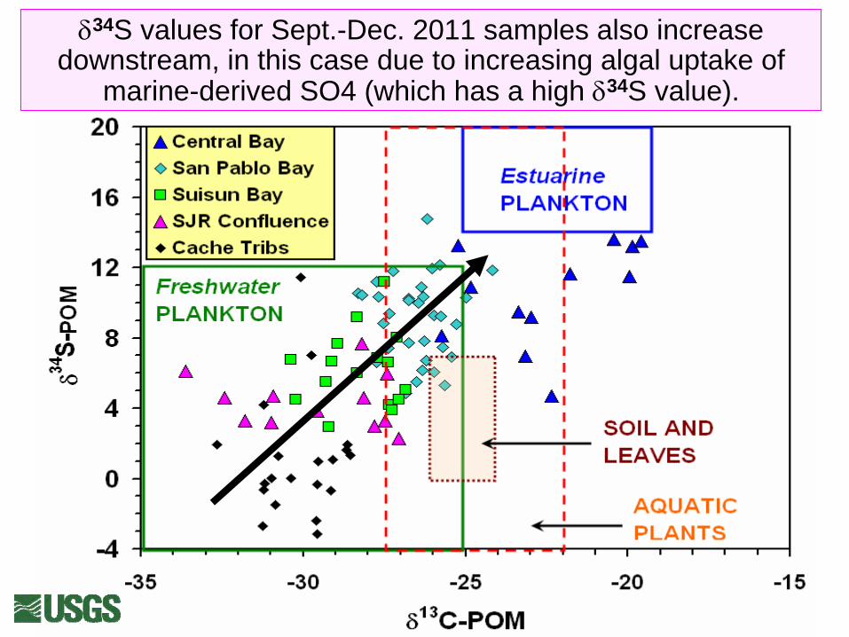
δ34S values for Sept.-Dec. 2011 samples also increase downstream, in this case due to increasing algal uptake of
marine-derived SO4 (which has a high δ34S value).

2011
2006
This slide and the next compare the compositions of POM from September to December, for 2011 (upper) and 2006 (lower).
C:N values for fall 2006 are much higher than for fall 2011, indicating that a much larger percent of the POM in 2006 is probably derived from soil/leaves and/or macrophytes.
δ13C-POM
δ13C-POM
C:N
-PO
MC
:N-P
OM

δ13C-POM
δ15 N
-PO
M
δ13C-POM
δ15 N
-PO
M
δ13C-POM
δ34 S
-PO
M
δ13C-POM
δ34 S
-PO
M
2011
2006

δ13C-POM
δ15 N
-PO
M
δ13C-POM
δ15 N
-PO
M
δ13C-POM
δ34 S
-PO
M
δ13C-POM
δ34 S
-PO
M
2011
2006δ13C-POM
δ15 N
-PO
M
δ13C-POM
δ15 N
-PO
M
δ13C-POM
δ34 S
-PO
M
δ13C-POM
δ34 S
-PO
M
2011
2006
These 2 sets of paired POM box plots (and the previous set of paired plots) show HUGE differences in POM sources and quality, and biogeochemical processing of C-N-S, for 2006 vs 2011.
The data can be used to estimate relative percentages of different sources and quality of POM for each sample.
Now let’s look just at LSZ samples, just for Sept. and Oct. – since these are the conditions specified in the Report’s predictive model.
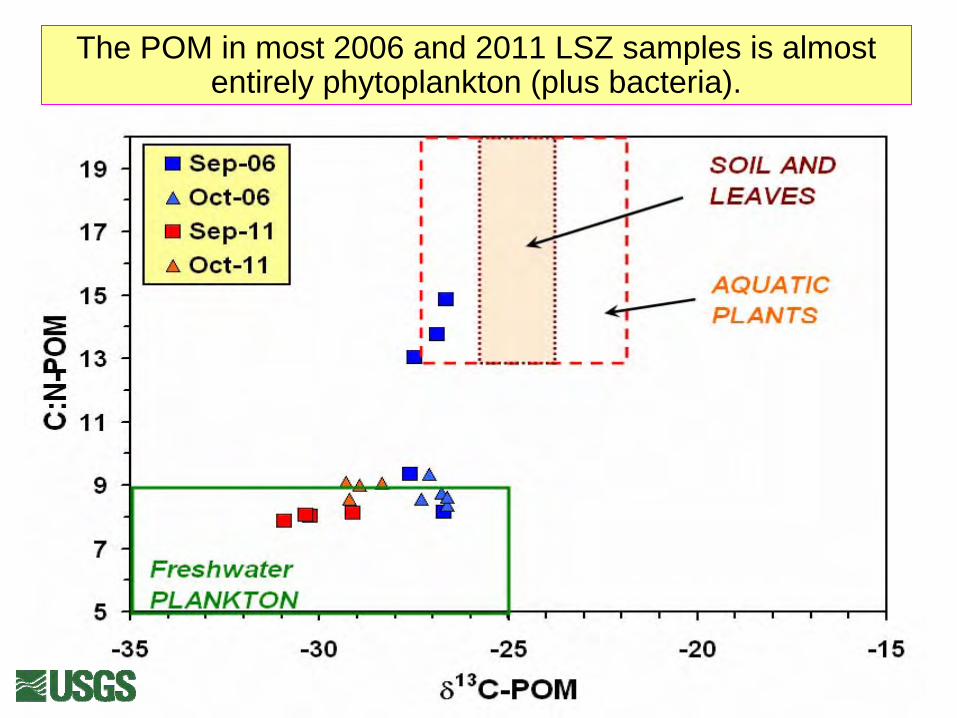
The POM in most 2006 and 2011 LSZ samples is almost entirely phytoplankton (plus bacteria).
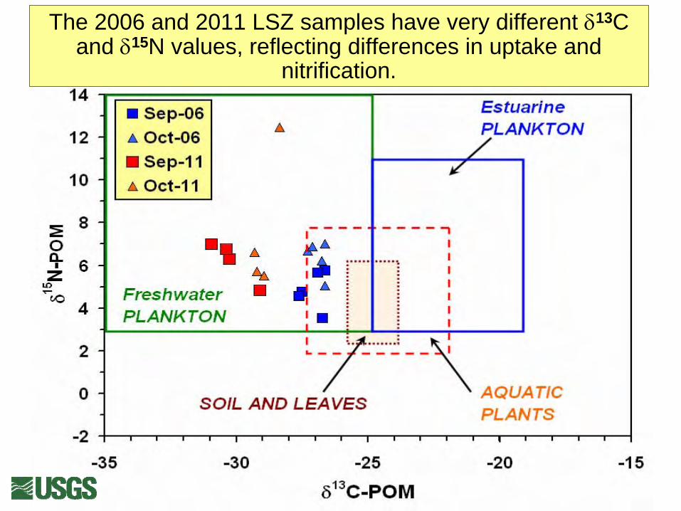
The 2006 and 2011 LSZ samples have very different δ13C and δ15N values, reflecting differences in uptake and
nitrification.
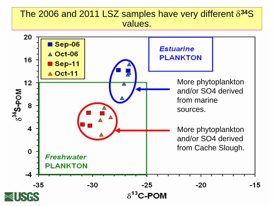
More phytoplankton and/or SO4 derived from Cache Slough.
More phytoplankton and/or SO4 derived from marine sources.
The 2006 and 2011 LSZ samples have very different δ34S values.
The Synthesis Report focused on data from the IEP EMP and DFG FMWT programs. In contrast, all the isotope samples and data (except for Cache Slough sites) shown in this presentation were piggybacked onto the USGS Polaris program.
Therefore, the Polaris dataset provides a different set of hydrology and chemistry data to test model predictions.
Hence, we have produced a table (like Table 5 in the Synthesis Report) that compares the values of various abiotic and biotic habitat parameters for September and October 2006 and 2011 USGS Polaris samples from LSZ sites.
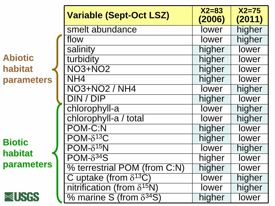
Variable (Sept-Oct LSZ) X2=83 (2006)
X2=75 (2011)
smelt abundance lower higherflow lower highersalinity higher lowerturbidity higher lowerNO3+NO2 higher lowerNH4 higher lowerNO3+NO2 / NH4 lower higherDIN / DIP higher lowerchlorophyll-a lower higherchlorophyll-a / total lower higherPOM-C:N higher lowerPOM-δ13C higher lowerPOM-δ15N lower higherPOM-δ34S higher lower% terrestrial POM (from C:N) higher lowerC uptake (from δ13C) lower highernitrification (from δ15N) lower higher% marine S (from δ34S) higher lower
Abiotic habitat parameters
Biotic habitat parameters

Predictions for X2 scenarios 85 km 81 km 74 km
Year used to test prediction
2010 2005, 2006 2011 Variable (Sep-Oct) (X2=85) (X=83,82) (X2=75)
Dynamic Abiotic Habitat Components Average Turbidity in the LSZ Lower Moderate Higher Average Ammonium Concentration in the LSZ Higher Moderate Lower Average Nitrate Concentration in the LSZ Moderate Moderate Higher Dynamic Biotic Habitat Components Average Phytoplankton Biomass in the LSZ (excluding Microcystis) Lower Moderate Higher
Green means that data supported the prediction.Red means the prediction was not supported.No shading indicates there were no data to assess.
Modified from Table 5, to only show variables where USGS Polaris LSZ data showed different relations between predictions and outcomes.
**for the next slide, chlorophyll-a was used as a proxy for phytoplankton biomass for Polaris comparisons.

Variable (Sept-Oct LSZ)Table 5:X2=83 (2006)
Table 5:X2=75 (2011)
X2=83 (2006)
X2=75 (2011)
turbidity moderate higher higher lowerNO3+NO2 moderate higher higher lowerNH4 moderate lower higher lowerchlorophyll-a moderate higher lower higher
Model supported
Model not supported
USGS Polaris data
IEP EMP and DFG FMWT data
For these 4 variables, Polaris data showed a different relation between X2 model predictions and outcomes than the Table 5 data.
No data to assess

Comments on report recommendations:
“Determine the correct spatial and temporal scale or scales for monitoring and other studies.”
The 4 variables where Polaris data showed a different relation between model predictions and outcomes than produced with the report datasets confirms the need for additional, perhaps more “tidally representative”, datasets for developing and testing models.
We are currently investigating the effect of flow, tides, and effluent concentrations on nutrient concentrations, uptake, and nitrification – using isotopes, chemistry, and DSM2/RMA modeling tools.
Few Delta monitoring programs sample only on ebb tides (e.g., Foe NH4 study, Kendall Slough study, Dugdale 2 Rivers study, Parker MC study). These studies sample mid-channel, and are a useful complement to other monitoring programs that are less concerned about sampling on the same outgoing tidal cycle, and sample at different locations within the channel.
The next slides show oscillations in chemistry -- probably due largely to tides -- that can bias interpretation of datasets confined to the LSZ.
USGS Polaris data
Golden Gate SJR Rio VistaPinole
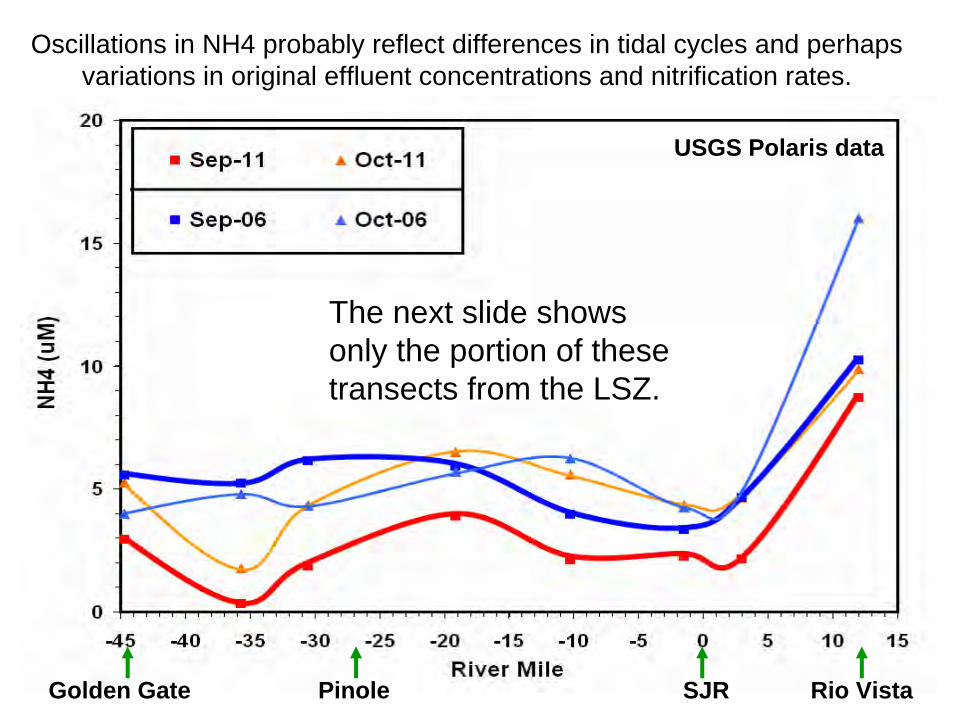
Oscillations in NH4 probably reflect differences in tidal cycles and perhaps variations in original effluent concentrations and nitrification rates.
The next slide shows only the portion of these transects from the LSZ.
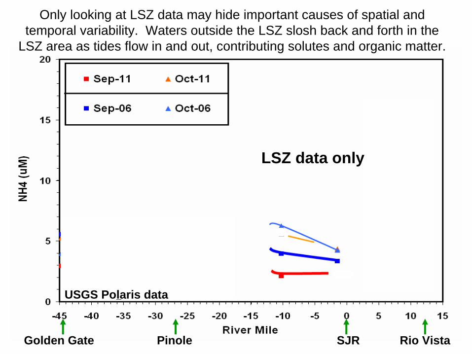
Only looking at LSZ data may hide important causes of spatial and temporal variability. Waters outside the LSZ slosh back and forth in the
LSZ area as tides flow in and out, contributing solutes and organic matter.
Golden Gate SJR Rio VistaPinole
LSZ data only
USGS Polaris data
Golden Gate SJR Rio VistaPinole
USGS Polaris data
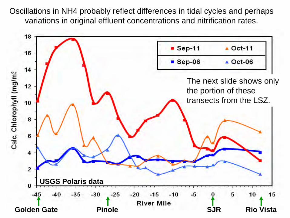
Oscillations in NH4 probably reflect differences in tidal cycles and perhaps variations in original effluent concentrations and nitrification rates.
The next slide shows only the portion of these transects from the LSZ.

2011
2006
Golden Gate SJR Rio VistaPinole
LSZ data only
Only looking at LSZ data may hide important causes of spatial and temporal variability, especially when not sampling all sites on ebb tides. Some Polaris
samples are collected on outgoing tides each month.
USGS Polaris data
Comments on report recommendations (con’t):
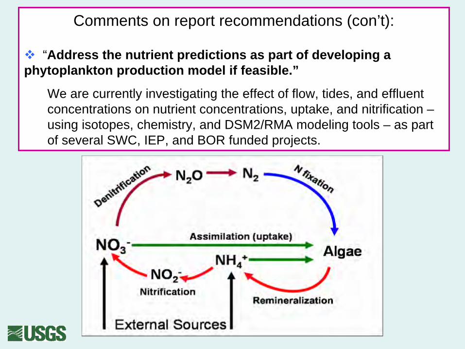
“Address the nutrient predictions as part of developing a phytoplankton production model if feasible.”
We are currently investigating the effect of flow, tides, and effluent concentrations on nutrient concentrations, uptake, and nitrification – using isotopes, chemistry, and DSM2/RMA modeling tools – as part of several SWC, IEP, and BOR funded projects.

Comments on report recommendations (con’t):
“Future iterations of this report should begin incorporating additional years of existing data into analyses in addition to new data.”
We have isotope, chemistry, and DSM2 data for 5 falls with a range of flows (2006, 2007, 2008, 2009, 2011), which could be used to test the robustness of patterns seen in the current study. Fall 2012??
We are currently investigating the effect of flows and effluent concentration on isotopes, chemistry, etc for 1990-2011, as part of an IEP-2010 study.
“All seasons should also be addressed.”We have isotope, chemistry, and DSM2 data for 3 spring/summers with a range of flows (2007, 2009, 2011); we have archived isotope samples for spring/summer 2012 – and hope for continued funding for 2013.
We are currently investigating the effect of flows and effluent concentration on isotopes, chemistry, etc for 1990-2011, as part of an IEP-2010 study.
Wet
Ab. Normal
Bl. Normal
Dry
Crit. Dry
(modified from Feyrer et al. 2010)
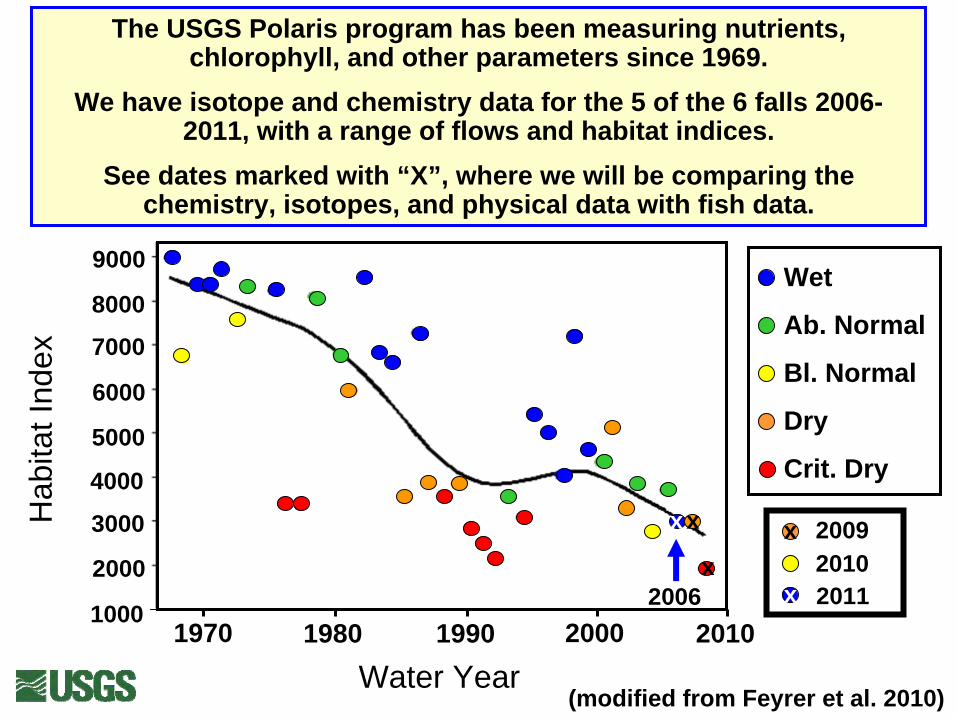
The USGS Polaris program has been measuring nutrients, chlorophyll, and other parameters since 1969.
We have isotope and chemistry data for the 5 of the 6 falls 2006- 2011, with a range of flows and habitat indices.
See dates marked with “X”, where we will be comparing the chemistry, isotopes, and physical data with fish data.
200920102011
x
x1000
2000
3000
4000
5000
6000
7000
8000
9000
Water Year1970 2010200019901980
Hab
itat I
ndex
2006x
xx

Conclusions:
These two different high-flow falls had very different chemical and isotopic responses, with the higher-flow fall 2011 showing much more frequent and larger phytoplankton blooms and substantially higher-quality organic matter, derived in part from the Cache/Yolo region.
The C-N-S isotopes of the POM are sensitive to changes in salinity, nutrient sources, extent and type of C-N-S cycling, geographic sources of the POM, quality of the organic matter, etc. – making them useful tracers of habitat environmental quality conditions.
Comparison of September and October LSZ data provided by the USGS Polaris program for 2006 and 2011 showed many differences between important biotic and abiotic variables used in the X2 predictive model in the Synthesis Report.
Some of the USGS Polaris LSZ data showed different relations between X2 model predictions and outcomes than in the Report, showing the need for larger and more representative datasets to further test model predictions.
Isotope-related parameters that showed strong differences between 2006 and 2011 may be useful tracers of important habitat characteristics; the observed patterns should be tested with isotope data from other falls with a range of flows, after first formulating predictions for different flow regimes.
Thanks to:
(1) the USGS RV Polaris team for letting us piggyback our isotope sampling on their monitoring program 2006-2012, and for providing the chemistry for the samples (http://sfbay.wr.usgs.gov/);
(2) Brian Bergamaschi (USGS) and his team for providing boats and skippers for our “Slough project” and FLaSH project sampling trips, 2011-12.
(3) Randy Dahlgren (UCD) for the chemistry data for “Slough project” samples.
(4) Our funding sources for this study:USGS National Research Program Bay-Delta (CALFED) ProgramInteragency Ecological ProgramBureau of Reclamation