Comparison of proposals for the future aeronautical

Ilmenau University of Technology

and

Institute of Communications and Navigation,German Aerospace Center (DLR)

Master Thesis

Haider Abdulkarim

Comparison of Proposals for the FutureAeronautical Communication System LDACS

Supervisors: Prof. Dr.-Ing. Giovanni Del Galdo

Dipl.-Ing. Ulrich Epple, Dr.-Ing. Michael Schnell

Faculty: Electrical Engineering and Information Technology

Research Group: Digital Broadcasting Research Laboratory

Date: 6 December 2012

cale5049

Schreibmaschinentext

cale5049


cale5049


urn:nbn:de:gbv:ilm1-2013200010

Abstract

For meeting future capacity requirements in aeronautical communications, a new air-

ground data link is needed. The European organization for the Safety of Air Naviga-

tion, EUROCONTROL, funded the development of two proposals for such a system.

The first proposal, called LDACS1, is a digital broadband OFDM-based system, which

was developed at the Institute of Communications and Navigation, DLR. The second

proposal, LDACS2 is developed by a project team consisting of EGIS AVIA, Helios,

SWEDAVIA and others. LDACS2 follows a single-carrier approach with GMSK modu-

lation. Both systems intend to operate in the aeronautical part of the L-band (960-1164

MHz). However, this frequency band is already utilized by different aeronautical legacy

systems, such as civil navigation aids DME or military communication systems (joint

tactical information distribution system, JTIDS). Furthermore, LDACS is exposed to

airborne co-site interference. A crucial issue in the selection process for one of the

LDACS systems is to guarantee the co-existence between LDACS and the legacy sys-

tems. On the one hand, it has to be verified that LDACS has only minor influence

onto the legacy systems. On the other hand, a reliable operation of LDACS in the

presence of interference has to be guaranteed.

In this master thesis, the performance of LDACS2 is analyzed. This task comprises

some theoretical considerations for investigating system features like capacity, spectral

efficiency, scalability, and the possible number of simultaneous users. The results show

the limitation of the offered bit rates per users due to the limited system bandwidth.

However, for low-to-moderate bit rates user demands, the offered bit rates are within

acceptable ranges. The main part of this work comprises the implementation of the

LDACS2 system according to the specification in the simulation software. This covers

the entire physical layer and the basic parts of higher layers. Special emphasis is put

on the implementation and evaluation of effective channel equalization algorithms and

channel coding schemes. Apart from AWGN channels, realistic aeronautical channel

models are also applied. It turns out that the particular channel coding schemes, pro-

posed in the specification, are not sufficiently robust. Other coding schemes that are

more suited for such channel conditions are proposed and show large enhancements in

the overall system performance. In addition, the robustness of LDACS2 against inter-

ferers from other aeronautical system, the DME, is investigated. The study shows that

LDACS2 system performs well against this type of interference for low-to-moderate in-

terference duty-cycles. On the other hand, interference from LDACS2 on a DME

system is negligible due to the relatively low transmission power of the LDACS2 com-

pared to the DME interrogator. The final task is to compare LDACS2 to LDACS1 in

terms of performance.

Acknowledgment

After completion of my Master thesis I wish to express my sincere gratitude to my su-

pervisor Professor Dr. Giovanni Del Galdo for his continuous support and Dr. Alexan-

der Ihlow and Mario Lorenz for their patient reviewing of this work. A special thank

goes to my mentor Dipl. Ing. Ulrich Epple who continuously supported and advised me

during the research period and also for his patience in reviewing the thesis afterwards.

I also would like to express my particular gratitude to the German Academic Exchange

Service (DAAD), who made my dream come true by granting me a scholarship to

pursue my master studies in Germany. The DAAD family continuously supported me

in a friendly manner. They introduced me to the German life and culture and made

me feel like living in my home country.

My gratitude goes also to the German Aerospace Center (DLR) and all the wonderful

colleagues and the administration there, who made me feel at home in Bavaria and

inspired me with their knowledge.

Studying in the university of Ilmenau was a great experience and source of enrich-

ment. Thanks to all my Professors for their interesting courses they offered us, which

I definitely will gratefully remember.

I dedicate my work to my mother and father, who never stopped motivating and

stimulating me. They were supportive and extremely caring for me. They made it

possible for me to acquire the best education. Though my thanks might not suffice, I

hope that I will be able to do something for them in return one day.

Last, but by no means least, I would like to thank my brother, my friends in Iraq,

at TU Ilmenau, in the lovely city of Munich, in Germany and the rest of the world.

They gave me support and encouragement and inspired me to keep learning. A special

thanks goes to Frau and Herr Doerr. When living with them in Seefeld, I experienced

the most kindness and generosity.

Contents i

Contents

1 Introduction 1

1.1 Background and State of The Art . . . . . . . . . . . . . . . . . . . . . 2

1.2 Methodology . . . . . . . . . . . . . . . . . . . . . . . . . . . . . . . . 3

1.3 Aeronautical Communication Demands . . . . . . . . . . . . . . . . . . 4

1.3.1 LDACS2 Layers . . . . . . . . . . . . . . . . . . . . . . . . . . . 5

1.3.2 LDACS2 Physical Layer Specifications . . . . . . . . . . . . . . 6

1.3.3 LDACS2 MAC Sublayer Specifications . . . . . . . . . . . . . . 9

1.4 LDACS2 Air Interface . . . . . . . . . . . . . . . . . . . . . . . . . . . 12

1.4.1 Radio Frequencies . . . . . . . . . . . . . . . . . . . . . . . . . . 13

1.4.2 Channel Bandwidth . . . . . . . . . . . . . . . . . . . . . . . . 14

1.4.3 Co-channel spacing between near ACs . . . . . . . . . . . . . . 15

2 LDACS2: The Transmitter 16

2.1 Channel Coding, Interleaving and Multiplexing . . . . . . . . . . . . . 16

2.2 GMSK Modulation in Theory . . . . . . . . . . . . . . . . . . . . . . . 17

2.3 GMSK Modulation . . . . . . . . . . . . . . . . . . . . . . . . . . . . . 19

3 Aeronautical Channel Models 25

3.1 Channel Modeling . . . . . . . . . . . . . . . . . . . . . . . . . . . . . . 25

3.2 Aeronautical Channel Characterization . . . . . . . . . . . . . . . . . . 28

3.2.1 En-route . . . . . . . . . . . . . . . . . . . . . . . . . . . . . . . 30

3.2.2 Taking-off/Landing . . . . . . . . . . . . . . . . . . . . . . . . . 32

3.3 Interference from Legacy Systems . . . . . . . . . . . . . . . . . . . . . 33

4 LDACS2 Receiver 35

4.1 GMSK Demodulation . . . . . . . . . . . . . . . . . . . . . . . . . . . . 35

4.1.1 Channel Estimation . . . . . . . . . . . . . . . . . . . . . . . . . 38

4.1.2 Matched Filter . . . . . . . . . . . . . . . . . . . . . . . . . . . 41

4.1.3 Maximum Likelihood Sequence Estimator (MSLE) . . . . . . . 41

Master Thesis Haider Adbulkarim

Contents ii

4.1.4 The Viterbi Algorithm in the LDACS2 Receiver . . . . . . . . . 43

4.2 Mitigating Fading Channel Effects . . . . . . . . . . . . . . . . . . . . . 45

4.2.1 Forward Error Correction . . . . . . . . . . . . . . . . . . . . . 46

4.2.2 Interleaving . . . . . . . . . . . . . . . . . . . . . . . . . . . . . 48

5 LDACS2 Performance and Capacity 51

5.1 LDACS2 Performance under Aeronautical Channel Models . . . . . . . 51

5.1.1 LDACS2 Simulator . . . . . . . . . . . . . . . . . . . . . . . . . 51

5.1.2 LDACS2 Performance in AWGN . . . . . . . . . . . . . . . . . 52

5.1.3 LDACS2 Performance in ENR Channel . . . . . . . . . . . . . . 58

5.1.4 LDACS2 Performance in the the TMA Channel . . . . . . . . . 62

5.1.5 DME Co-site Interference . . . . . . . . . . . . . . . . . . . . . 65

5.1.6 Time and Frequency Error Performance . . . . . . . . . . . . . 66

5.2 LDACS2 Capacity . . . . . . . . . . . . . . . . . . . . . . . . . . . . . 68

5.3 LDACS2 vs. LDACS1 Performance . . . . . . . . . . . . . . . . . . . . 70

5.3.1 LDACS1 Parameters . . . . . . . . . . . . . . . . . . . . . . . . 70

5.3.2 Performance Comparison . . . . . . . . . . . . . . . . . . . . . . 72

6 Conclusions 75

6.1 Implementaion . . . . . . . . . . . . . . . . . . . . . . . . . . . . . . . 75

6.2 Results . . . . . . . . . . . . . . . . . . . . . . . . . . . . . . . . . . . . 76

6.3 Design Drawbacks . . . . . . . . . . . . . . . . . . . . . . . . . . . . . . 77

6.4 Future Work . . . . . . . . . . . . . . . . . . . . . . . . . . . . . . . . . 77

Bibliography 83

List of Figures 86

List of Tables 87

Erklarung 88

Theses of the Master Thesis 89


1 Introduction 1

1 Introduction

The traditional aeronautical communication is using the very high frequency (VHF)

band for more than 70 years for analog radio systems. However, this band is already

saturated. Besides, the analogue communication itself does not serve best in terms of

spectral efficiency and the offered capacity. Hence, the need to develop a more efficient

system capable of coping with the increasing data traffic (and number of aircrafts) has

launched the Future Communication Study (FCS) in 2002. The project is proposed

by the National Aeronautics and Space Administration (NASA) and the European

Organization for the Safety of Air Navigation (EUROCONTROL). At the end of this

project, two candidates have been selected by the International Civil Aviation Orga-

nization (ICAO) for a future digital air-ground communication systems. Those can-

didates are L-band Digital Aeronautical Communications System, Type1 (LDACS1)

and L-band Digital Aeronautical Communications System, Type2 (LDACS2).

In order to select the final system proposal, independent studies on both of the pro-

posals have to be carried out. Also, the performance of the two proposals has to be

tested against different scenarios (traffic load, number of users) as well as the effects

of Additive White Gaussian Noise (AWGN) and fading channels on the performance

of the system. The well-known figure of merit, Bit Error Rate (BER), is chosen to

evaluate the system performance. In this work, the focus is put on the LDACS2 pro-

posal because of its low bandwidth utilization and relatively simple system structure

for both the transmitter and the receiver blocks.

In this chapter, a brief history on the development of LDACS2 as well as a summary

about the related contributions is given. Then, an overview of the general LDACS2

physical layer parameters and specifications is given. Later, the Medium Access Con-

trol (MAC) layer structure is depicted in summary, highlighting the main parameters

that are used in simulating LDACS2 transmitter and receiver in the Chapters 2 and

4, respectively.


1 Introduction 2

Figure 1.1: Evolution of aeronautical datalinks [4].

1.1 Background and State of The Art

Due to the tremendous air traffic increase in the last century, the need for more reli-

able and efficient communication between the aircrafts and ground stations emerged.

Among other requirements, the need for data communication rather than only voice

communication, higher data rates and better spectral efficiency are the most chal-

lenging burdens. In 2002, NASA and EUROCONTROL launched the project FCS

to develop a new air-ground communication system capable to meet those emerging

requirements [1]. The final selection by the ICAO voted for, among other candidates,

two final proposals. Those are LDACS1 and LDACS2. They will be operated in the L-

band (960 - 975 MHz), which is currently used by the Aeronautical Radio-navigation

Services (ARS). The finally selected candidate is to be deployed in the year 2020.

While LDACS1 is based on Frequency Division Multiple Acces (FDMA), LDACS2

is a Time Division Multiple Access (TDMA) system. LDACS2 is evolved from All

Purpose Multichannel Aviation Communication System (AMACS), which is in turn

derived from the well known GSM system, as shown in Figure 1.1.

The selection process of the final LDACS system proposal is shown in Figure 1.2 [2].

Although the testing and evaluation phase of the selection process is important, very

few contributions have been made to this field. In [1], for example, the authors study

the impact of LDACS on legacy systems that still work in L-band. The authors finally

conclude that the interference from LDACS2 will be higher than that of LDACS1. In

[3], the authors characterize the interference sources. They study the detection and

mitigation techniques for LDACS1 only but not for LDACS2.


1 Introduction 3

Figure 1.2: Selection process of the final LDACS proposal [2].

In [4], an independent theoretical comparison between the two proposals is provided.

The comparison is done in terms of scalability, spectral efficiency, type of data traffic

offered (symmetric vs. asymmetric) and possible interference from GSM base stations.

However, their comparison is based not on simulation scenarios, but only on theoretical

aspects. For the sake of independent comparison, our work presents an intensive study,

implementation and evaluation of the proposed LDACS2.

1.2 Methodology

This work investigates the LDACS2 specifications and performance of the physical

layer and MAC sublayer. In the following sections of Chapter 1, LDACS2 layers as

summarized. The focus is made on the physical and MAC layers because of their influ-

ence on the system performance. In Chapter 2 the LDACS2 transmitter is described.

The first contribution of this thesis is the implementing and validating of the LDACS2

transmitter. Then, the proposed channel coding are mentioned in brief. In Chapter

3 the channel models are introduced. Then, the commonly used aeronautical channel

models are categorized. Afterwards, the DME system is described. The outcome of

Chapter 3 is essential in evaluating the LDACS2 performance.

The other main contribution of this thesis is the implementation of LDACS2 receiver, as

described in details in Chapter 4. Since the LDACS2 specifications do not describe the

implementation of both the transmitter nor the receiver, large efforts have been ded-

icated to implement the LDACS2 simulator, taking the strict LDACS2 specifications

into account. The concrete system model is then illustrated and the implementation

issues are discussed in details. Special techniques to overcome implementation issues

are also discussed. The channel coding and decoding are briefly discussed at this chap-


1 Introduction 4

ter, with special emphasize on the coding parameters that directly affect the channel

coding performance.

The other major contribution of this master thesis is presented in Chapter 5. In this

chapter, the aeronautical channel models presented in Chapter 3 are adapted into the

LDACS2 simulator. Then, the LDACS2 performance is evaluated under those channel

models. Based on the system performance, more efficient channel coding parameters

are suggested and validated which shows a considerable improvement in the perfor-

mance. Besides, modifying the frame structure to cope with rapid fading channels is

also proposed and validated through results. The LDACS2 reliability against timing

and frequency error is tested and the results are presented. Finally, a comprehensive

study on the practical LDACS2 capacity and actual information bit rates is presented.

1.3 Aeronautical Communication Demands

In this section the following two questions are answered: what kind of information

does the aeronautical communication support? and what are main the challenges in

aeronautical communication air-ground data-links?

To answer the first question, it is mandatory to consider the increasing demand for

air traveling. As a consequence, the demand to maintain vital services to the airliners

is increased. Among those services, Air Traffic Control (ATC) is the most important

one. With ATC services, it is possible to control the traffic of the increasing number of

aircrafts and to avoid collisions. Besides, other vital information are supported to the

pilots, including weather informations, navigation and flight orders within the airport.

Airline Operational Control (AOC) data maintains real-time traffic managements of

hundreds of aircrafts and thousands of crew members to avoid delays and cancellation

[6]. Obviously, for ATC and AOC data services, there are strict latency requirements

(in the range of ms) and a certain probability that those messages are successfully

transmitted.

Taking into consideration the speeds at which the airplanes cruising, there are basically

two main dissimilarities between aeronautical communication links and land commu-

nication links. The first one is the long distances (large cell sizes) that need to be

covered [4]. Considering the widely implemented IEEE 802.11 standard (WIFI) as an

example, its coverage area is limited. Even the IEEE 802.16 (WiMAX) can only serve


1 Introduction 5

up to 3 km in suburban areas. On the other hand, aeronautical data-links should cover

up to 360 km, which makes the implementation of WiMAX unpractical. The second

major difference is the speed of the aircraft. While WiMAX is designed to support a

maximum velocity of up to 120 km/h, the cruising speed of a 747 airliner would be

in the range of 900 km/h, resulting in a very high Doppler spread which reduces the

spectral efficiency, as seen in Chapter 3.

As a conclusion, it is not feasible to use the existing ground communication technolo-

gies for aeronautical communications. However, LDACS2 makes use of some of the

favorable features of existing technologies and adapts them accordingly. The LDACS2

is designed to be configured with flexibility in mind. That is, LDACS2 can serve point-

to-point services (aircraft-to-aircraft or aircraft-to-ground station) as well multi-cast

services (ground station-to-aircraft). In the current specifications, the focus is made on

aircraft-to-ground and vise versa, with the possibility of extension to aircraft-to-aircraft

in the future.

After selecting the final LDACS proposal, the old radios have to be kept at the begin-

ning. There will be a step by step superseding of the old system. For example, the

old VHF is still used for voice and LDACS for data (and also voice later on). Time

path, however, is not yet clear, and probably it will be introduced between the years

2020− 2030.

1.3.1 LDACS2 Layers

In this section, the LDACS2 layers are discussed, with focusing on the layers that

are related to this work. Since the performance of LDACS2 depends on the physical

and MAC layers, this work focuses on those layers. It should be mentioned that

voice services will also be supported, but its implementation is not yet specified in the

specifications.

The general LDACS layers are illustrated in Figure 1.3. The physical layer, as the

name suggests, deals with all transmission concepts as well as the channel coding.

The MAC sublayer defines the framing structure of LDACS2 and time synchroniza-

tion. The Data Link Sublayer (DLS) relies on the MAC sublayer to ensure that the

user messages are delivered without errors through establishing and releasing of DLS

connections. The offered connections are connection-oriented (point-to-point) and con-

nectionless (broadcast services). The LDACS2 Service Sublayer (LSS) provides flexible


1 Introduction 6

Control User data

Service sublayer

Data link sublayerL

ME

Physical layer

Lin

kM

anag

emen

t L

ayer

MAC sublayer

Figure 1.3: LDACS2 layers.

burst formatting for the MAC sublayer framing structure and is also responsible of the

transmission and reservation protocols over the MAC sublayer. Finally, the Link Man-

agement Entity (LME) is responsible for establishing and maintaining the connections.

The entities MAC, LSS, DLS and LME together represent the Link Management

Layer (LML), which is also responsible for the login and handover mechanisms. Since

the performance of the physical layer and MAC sublayer determines the overall perfor-

mance of LDACS2, this work focus on the physical and MAC entities. However, the

other sublayers functions are described in details in [2].

1.3.2 LDACS2 Physical Layer Specifications

In this section, the physical layer highlights of LDACS2 are demonstrated. It was

adapted from the AMACS. LDACS2 is operated in the lower part of the L-band,

namely 960−975 MHz, as shown in Figure 1.4. The standard [2] inherits some features

from its ancestors, see Figure 1.1. For example, the Time Division Duplexing (TDD)

is adopted from AMACS. Besides, the principle of dedicated and on-demand slots is

extended from AMACS to LDACS2. The tendency to operate in a less congested


1 Introduction 8

then Tb is defined as

Tb =1

Rb

= 3.69 µs. (1.3)

The name MSK comes from the fact that MSK could be seen as a form of Frequency

Shift Keying (FSK) with frequency deviation ∆f defined as [7]

∆f = f1 − f2, (1.4)

where f1 and f2 are the two LDACS2 frequency components after modulation. To be

able to recover the data at the receiver side, ∆f should be

∆f =1

2Ts=Rb

4. (1.5)

(1.5) states that the minimum shift in frequency should be Rb/4 to recover the signal

without ambiguity, and hence the name minimum shift keying.

In LDACS2 the resulting frequency components can be written as

f1 = fc +Rb

4,

f2 = fc − Rb

4.

(1.6)

This is equivalent to have fc swinging between two values, as seen in Figure 1.5. That

is, a logical 1 increases the phase by 90◦ over Tb while a logical 0 decreases the phase

by 90◦.

The modulation index m is then related to Ts by [8]

m = ∆fTs = 0.5 . (1.7)


1 Introduction 9

Figure 1.5: MSK modulated signal [5].

To further limit the system bandwidth B in GMSK, the MSK output signal is filtered

with a Gaussian low pass filter. B is then limited to 200 kHz and the resulting spectrum

decays faster after the system bandwidth than that of the MSK spectrum. However,

since B is smaller than Rb, Nyquist sampling theorem is violated. As a result, Inter

Symbol Interference (ISI) is introduced in the signal. This ISI is easily mitigated at

the receiver, as seen in Chapter 4.

LDACS2 specifies the normalized-bandwidth-time product BT to be 0.3, according to

[8]

BT =f3dBRb

= 0.3, (1.8)

where f3dB is the Gaussian filter one-sided bandwidth, which is equal to 81.25 kHz.

The LDACS2 transmit output power is set to 350 W at the ground station and 50 W

at the aircraft. After link budget calculations [2], the maximum radius of LDACS2 cell

size is 200 Nautical Mile (NM), where 1 NM is 1.852 km.

1.3.3 LDACS2 MAC Sublayer Specifications

In this section the main features of the LDACS2 MAC layer are covered. The main

architecture is adopted from the MAC layer of AMACS, with a fixed frame length of

1 s to accommodate high priority messages that should not be delayed. The frame

structure is TDD in the sense that either one of the communicating entities (the trans-

mitter or the receiver) is allowed to send or receiver at a given time. Each LDACS2

frame of 1 s is divided into five sections, namely UP1 and UP2 for the up-link, CoS1

and CoS2 for the down-link and the LoG2 section for logging in. The frame structure


1 Introduction 11

It is also possible that a slot is shorter than the basic slot. On the other hand, a burst

spanning multiple basic slots is used whenever the message is longer than one slot or

to contain multiple messages from the same user. Since there is one header and one

trailer in a single burst, there is less overhead in a burst than in a slot.

The UP1 and UP2 sections are used to transmit data from the GS to the AC. The

GS concatenates all of its messages into two continuous burst, one for each section.

Since it has control of its entire UP section, the GS transmits in bursts rather than

slots. Each UP burst spans a number of basic slots. That is, the minimum size of a

UP burst is two basic slots (13.33 ms), see Figures 1.8. The CoS1 section is used to

transmit high priority short messages from the AC to GS. The CoS1 slot (the slot in

CoS1 section) length is 1.11 ms (see Figure 1.9). If a user needs access to bursts for

long messages, it requests access to the CoS2 section during its assigned CoS1 slot and

it would be granted access to one or more slots in CoS2 section. While a CoS1 slot is

short, CoS2 slot has a length equivalent to the basic slot, see Figure 1.10. The log-in

procedure takes place in the LoG2 section. With a duration of 3.33 ms, the LoG2 slot

is used by the AC to have access to a CoS1 slot. The LoG2 slot structure is illustrated

in Figure 1.11.

To provide the maximum flexibility, the length of each section can be changed dynam-

ically according to the user demand. The total duration of the five sections is 1 s.

However, only the GS is allowed to change the sections length. When it intends to

modify the sections duration, the GS should notify all the logged-in aircrafts multi-

ple times with sufficient frames before the actual change in the frame structure takes

place; this is to ensure the high probability of all aircrafts to adapt to the new frame

structure. A summary of the LDACS2 frame parameters is given in Table 1.1.

Table 1.1: LDACS2 frame parameters.

Parameter Value

Frame length 1 sFrame duration 150 basic slotsSlot Duration 6.666 ms (basic slot)Bits / slot 1806 (basic slot)Duplexing half (uplink and downlink)


1 Introduction 12

Figure 1.8: UP slot, 3612 bits, 13.33 ms [2].

Figure 1.9: CoS1 slot, 300 bits, 1.11 ms [2].

1.4 LDACS2 Air Interface

In this section, a summary of the main LDACS2 transmission features is provided. The

transmission characteristics cover the radio frequencies, channel bandwidth as well as

the guard bands that should be maintained.


1 Introduction 13

Figure 1.10: CoS2 slot, 1806 bits, 6.66 ms [2].

Figure 1.11: LoG2 slot, 902 bits, 3.33 ms [2].

1.4.1 Radio Frequencies

Although the assigned frequency ranges from 960 - 975 MHz, a guard band of 500

kHz at the lower edge of the spectrum should be maintained. This is to protect

other communication systems that use the frequencies below 960 MHz (such as GSM

systems) from LDACS2 out-of-band radiation.


1 Introduction 14

Table 1.2: Channel bandwidth vs. various cell sizes.

Scenario Service No. of AC User Demand Channels required Total bandwidth

TMA(large) ATS and AOC 52 47 kbps 1 200 kHzEnroute(medium) ATS and AOC 64 55 kbps 1 200 kHzEnroute(large) ATS and AOC 204 188 kbps 2 400 kHz

1.4.2 Channel Bandwidth

The LDACS2 specification suggests a nominal channel bandwidth of 200 kHz. This is

supposed to be sufficient to serve the most operational scenarios. However, when there

is a need for more capacity per cell, channel aggregation should be used. When imple-

mented, two or more channels, each with a bandwidth of 200 kHz, serve as a virtual

single channel. This allows higher data rates to be achieved. Channel aggregation is

achieved by using a frequency reuse concept (from the GSM) in adjacent cells, allow-

ing more flexible frequency planning and saves frequency resources. The traffic load

of the cell will be shared among the channels. One way to achieve this is to use cell

segmentation (taken from GSM) by using sectorized antennas. An example of channel

aggregation is illustrated in Table 1.2

The minimum channel separation between two channels belonging to the same cell

should be at least 600 kHz to prevent interference between adjacent bands. However,

considering the minimum clearance distance between the GS and the nearest AC, the

minimum separation could be reduced to 400 kHz. Considering the example in [2]: with

200 kHz frequency separation, the two mobile stations have to be separated by 10 NM

(approximately 18.5 km). With a channel separation of 400 kHz, the AC receiver is

still able to demodulate the signal from the GS. In this case the two mobile stations

(considering two ACs) have to be separated by 0.23 NM (approximately 0.42 km),

which is far less the minimum allowable separation between any two ACs at a given

time.


1 Introduction 15

1.4.3 Co-channel spacing between near ACs

In this section, the case of two ACs working at the same channel frequency, but in

two different (adjacent) cells is considered. In this case AC1 is transmitting to GS1

while AC2 is receiving data from GS2. The goal is to determine the minimum distance

between the two ACs that lead to a successful demodulation of the received signal at

both of the ACs. The minimum spacing is found to be 80 NM to keep the Carrier to

Interference (C/I) at a maximum of 9 dB, according to Table 1.3 [2].

Table 1.3: Channel interference.

Interference Type Interference Ratio

co-channel interference 9 dBadjacent (200 kHz) interference −9 dBadjacent (400 kHz) interference −41 dBadjacent (600 kHz) interference −49 dB



2 LDACS2: The Transmitter

The LDACS2 specification retains some features from GSM: the reason behind this

is to simplify the physical implementation by using already existing technologies in

the market. This will help the developers to migrate to faster data rate services such

as EDGE or GPRS whenever higher traffic densities and increasing traffic demands

are desired. This chapter concisely reveals the LDACS2 transmitter structure, shown

in Figure 2.1. First, a brief description of the coding parameters suggested by the

specifications is listed. Then, an introduction into GMSK is presented and compared

to MSK. Later, the basic GMSK modulation steps are presented according to the

international GSM standards. The GMSK modulation is then used implementing the

LDACS2 transmitter using MATLAB simulation environment.

RS coderSymbol

interleaverConv. coder Bit interleaver

Framing,header and

trailer

GMSKmodulation

Informationbits

Modulatedsignal

Figure 2.1: LDACS2 general transmitter structure.

2.1 Channel Coding, Interleaving and Multiplexing

To protect the transmitted data against random and burst channel errors, channel

coding is used. The LDACS2 specification [2] specifies a concatenated coding scheme

to be used. It consists of inner and outer codes. The inner code is a convolutional code

(7, 171, 133), where 7 is the constraint length. This code has been already implemented



in DVB systems. It makes the transmitted signal robust against AWGN random errors.

The chosen code rate Rc = 3/4, which is accomplished using puncturing from a mother

Rc = 1/2 code. The outer coder is a Reed Solomon (RS) code. The specification

suggest the usage of RS(15, 11, 4) or RS(31, 23, 5). Between the two codes, a block or

diagonal interleaver exists. A bit interleaver is used after the inner coder to randomly

permute the convolutional-coded bits. This protects the bits against uncorrelated

errors over time. A comprehensive study on the coding and interleaving techniques is

presented in Section 4.2.

The multiplexing step simply accumulates the bits into a stream formatting prior to the

modulation step. This also includes attaching the flag bits (message type), ramp bits

(to reduce out of band emission), training sequence, Code Redundancy Check (CRC)

and guard bits. The guard bits length is equal to the maximum propagation delay

between the transmitter and the receiver. This maximum length is calculated based

on a maximum cell radius of 200 NM.

2.2 GMSK Modulation in Theory

As stated in Chapter 1, the GMSK modulation scheme is chosen as the proposed

modulation scheme for LDACS2. GMSK is a special form of MSK. The goal of MSK

modulation is to limit the maximum carrier phase transition between successive sym-

bols to π/2. As a result, there are no abrupt phase transitions, implying that the MSK

spectrum is band limited. To understand the GMSK modulation, the MSK modulation

is first considered. The MSK modulated signal, si (t) could be written as [12]

si (t) = aicos

(

πt

Ts

)

cos (2πfct) + bisin

(

πt

Ts

)

sin (2πfct), (2.1)

where ai and bi are Non-Return-To-Zero (NRZ) input bits, Ts is the symbol duration,

in seconds. The relationship between the I and Q components of MSK modulation is

seen in Figure 2.2.

Because of the Ts/2 s delay between ai and bi (Figure 2.3), only one of them can change

at a time. The effect of the term ai cos (πt/Ts) is to force the carrier term cos (2πfct) to

go to zero at the bit transition point (end of Tb) while the other carrier term sin (2πfct)



0 2 4 6 8 10 12−1

−0.5

0

0.5

1

Tb

Bit

lev

el

I = cos(2Πfct)

Q = sin(2Πfct)

Figure 2.2: MSK modulator fed with a sequence of ones. I lags Q by π/2. Each Tbincreases the phase by π/2.

lpf

lpf delay

cos 2π f tc

sin 2π f tc

S (t)i

Tb

ai

bi

Figure 2.3: MSK modulator.

is at its peak. The same discussion applies when the carrier cos (2πfct) is at its peak

while the other carrier term sin (2πfct) is forced by the term bi sin (πt/Ts) to go to

zero.

fc is chosen such that it has integer number of half cycles within each Ts. This assures

no phase discontinuity at the bit transition point.

Using trigonometry, (2.1) is rewritten as

si (t) =

cos(

2πfct ∓ πtTs

)

for ai = 1, bi = ±1,

cos(

2πfct ± πtTs

+ π)

for ai = −1, bi = ±1.(2.2)



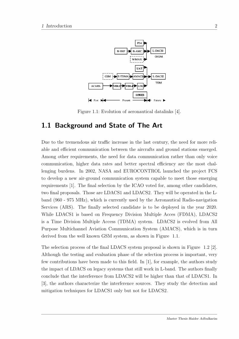
Equivalently

si (t) = cos

(

2πfct −aibiπt

2Tb+ θ

)

, (2.3)

where

θ =

0, for ai = 1,

π, for ai = −1.(2.4)

From (2.4), one concludes that since either ai or bi changes every Tb while the other is

kept constant, the maximum phase difference is limited to π/2, as seen Figure 2.4.

Recalling (1.5), the minimum frequency separation ∆f between two adjacent carriers

is Rb/4, in order for the synchronous detector at the receiver to detect the signal

without ambiguity.

In GMSK modulation, it was decided [13] to further limit the bandwidth of the base-

band pulse train by filtering the signal with a pre-modulation filter (Gaussian Filter).

The resulting output phase is very smooth compared to that of the MSK (Figure 2.4).

As a consequence, the GMSK occupied bandwidth B is narrower than that of MSK

(Figure 2.5). A comprehensive description of the GSMK modulation steps is given in

Section 2.3.

2.3 GMSK Modulation

A comprehensive description of the GSMK modulation steps is given in this section.

Following the GSM specification [9], there are basically four steps to modulate the

data bits (baseband representation is considered):



0 2 4 6 8 10 12 14 16 18 200

2

4

6

8

10

12

14

Tb

Ph

ase

Π/2

MSK

GMSK

Figure 2.4: For the same binary sequence, GMSK phase is smoother than MSK.

−300 −200 −100 0 100 200 300−40

−20

0

20

40

60

Frequency (kHz)

Mag

nit

ud

e (d

B)

GMSK

MSK

Figure 2.5: GMSK vs. MSK Spectrum. High attenuation for GMSK spectrum after200 kHz.

• Differential Encoding

The data bits di to be modulated are in the Return-to-Zero (RTZ) form (di =

[0, 1]). They are differentially encoded, to obtain di

di = di ⊕ di−1, where di ∈ {0, 1}. (2.5)



Then the input to the modulator becomes

ai = 1− 2di, where ai ∈ {−1, 1}. (2.6)

Note: the GSM specification assumes an infinite sequence of ones preceding the

actual burst start.

• Filtering

The output from the differential encoder ai, passes a Gaussian filter, whose im-

pulse response g(t) is given by

g (t) = h (t) ∗ rect(

t

Tb

)

, (2.7)

where ∗ denotes a convolution. And

rect

(

t

Tb

)

=

1Tb

for |t| < Tb

2,

0, otherwie.(2.8)

h (t) is defined as:

h (t) =exp

(

− t2

2σ2T 2

)

√2πσTb

, (2.9)

given

σ =

√

ln (2)

2πBTb. (2.10)



For GSM, as well as LDACS2 B is the 3dB bandwidth of the filter g (t), given

by:

B = 81.25 kHz and Tb = 3.69 µs.

• Modulated Signal Generation

The output signal x(t) from the filter g(t) is described as

x (t) =

√

2Ec

Tbcos(2πfct+ φ (t) + φ0), (2.11)

where Ec is the energy per modulating bit, φ(t) is the phase function and φ0 is

a random phase (constant during Tb).

• Phase Function

The phase function φ(t) is defined as

φ (t) =∑

i

aiπh(t)

∫ t−iTb

−∞

g (u) du. (2.12)

Since the ideal shaped Gaussian filter has an infinite bandwidth, it is not be realizable

in practice [10]. Instead, a practical approximation is to limit the time response of the

filter to a length of L, where L ≥ 3 is the number of samples per bit that represent

the Gaussian pulse. For GSM (as well as LDACS2), it is decided to choose L = 3Tb,

see Figure 2.6. That is, (2.7) is altered as

g (t) = g

(

t− LTb2

)

wl(t), (2.13)

where wl (t) is the windowing function used to limit the impulse response of the filter

g (t) to 3Tb, defined as



0 1 2 30

0.1

0.2

0.3

0.4

0.5

Tb

Am

pli

tude

Figure 2.6: Pulse shaping function g(t) is limited to 3Tb.

wl (t) =

1 for 0 ≤ t ≤ LTb,

0 otherwise,(2.14)

A closer look at (2.13) indicates that ISI is intentionally introduced into the signal.

This is because the symbol is now spread over a 3Tb period instead of 1Tb, see Figure

2.6.

However, this kind of ISI can be easily mitigated by using a Maximum Likelihood

Sequence Estimator (MLSE) equalizer at the receiver, as explained in Chapter 4.

In this work, the described GMSK modulator is implemented and tested using MAT-

LAB simulator. This GMSK modulation approach was chosen based on LDACS2

recommendation [2]. The implementation also include the channel coding, intreleaving

and the multiplexer. A comprehensive description of the coding and interleaving is

introduced in Chapter 4. The multiplexer step adds the header and trailer bits to

each user message, in order to construct the LDACS2 frame, as explained in Section

1.3.3.



The general LDACS2 transmission chain is demonstrated in Figure 2.7.

Channel coding& interleaving

Multiplexer Differentialencoder

GMSKmodulator

Modulatedcarrier x(t)

Informationbits

Figure 2.7: LDACS2 transmitter chain.



3 Aeronautical Channel Models

When studying communication systems, one of the most important factors to be con-

sidered is the transmission channel. The term ”channel” refers to the medium between

the transmitter and the receiver. In its simplest form, the channel is considered ideal

when the transmission occurs in the free space. That is, the free space path loss model

is assumed whenever there are no obstacles between the transmitter and the receiver.

In reality, the experienced channel effects are far from being ideal. Those effects are

caused by the relative motion between the transmitter and the receiver as well as the

existence of obstacles in between. Those obstacles introduce the so called multi-path

fading. The received signal level, attenuated by the path loss, additionally degrades

by the multi-path effect.

In this chapter, a brief introduction to the general wireless channel models is made.

Then, the experienced aeronautical channel models are characterized with a summary

of each channel model parameters. The outcome of this chapter will facilitate studying

and simulating the LDACS2 performance.

3.1 Channel Modeling

In this section, the free space path channel model is introduced. Then, channel fading

and multi-path effect is explained. The concept of channel modeling is then summa-

rized. The simplest form of the channel model assumes that the received signal is

only attenuated by the traveled distance and AWGN. The AWGN channel model is

assumed whenever the noise samples are statistically independent and follow a complex

Gaussian distribution with mean µ and standard deviation σ for both I and Q com-

ponents. The AWGN is generated at the receiver, basically due to the thermal noise

at the normal operation temperature. The Power Spectrum Density (PSD) of the



AWGN is constant which indicates that the noise is added up equally to all frequency

components of the original signal.

In addition to this added noise and following the simplest channel model, the free space

path loss model is assumed whenever there are no obstacles between the transmitter

and the receiver. Furthermore, the received signal does not suffer from reflection,

diffraction or scattering phenomena. Usually, this channel model is described by the

free space path loss Ls factor as follows

Ls (d) =

(

4πd

λ

)2

, (3.1)

where d is the distance between the transmitter and receiver, and λ is the wavelength

of the carrier frequency fc. As expected, Ls(d) grows for large values of d, fc, or both.

In reality, most of the wireless channels cannot be modeled by the simple free space

path loss model. The reason is that besides the path attenuation, the receiver receives

multiple copies of the original signal via different paths, which is known as multi-path

propagation or fading. Those types of channel models are widely used in the model-

ing of communication channels because they can describe the channel characteristics

efficiently.

There are mainly two types of fading:

1. Large scale fading : The fading occurs due to the relative motion between

the transmitter and the receiver, because the transmitted signal suffers from

being blocked by large building, hills, etc. The large scale fading (also called

shadowing) is a function of d. The path loss Lp(d) is described by the nth-power

law [14]) as

Lp(d)(dB) = Lp(d0) + 10n log

(

d

d0

)

, (3.2)

where Lp(d0) is mean path loss at the reference distance d0 and n is the path loss

exponent.



Figure 3.1: Large fading (shadowing) vs. small scale (multi-path) fading [14].

Figure 3.2: Multipath power delay profile example [14].

2. Small scale fading: The fading effect in this case is mainly due to the multi-

path reflected versions of the signal, which vary in the phase and the amplitude.

It is called small scale because of the large variation in the fading effect due

to very small displacements (in terms of λ/2) when either the transmitter or

the receiver moves. Due to the multi-path components, the total effect of the

received signal components may vary between constructive and destructive. This

is because of the variations in the phase of the multiple reflected components.

The effect of both large and small scale fading is illustrated in Figure 3.1.

To simplify channel modeling, and since the received signal is actually the effective

sum of the reflected replicas of the transmitted signal, the channel is often described

as a multi-tap profile. Each received component is described by its relative arrival time

and the intensity of the respective component, as shown in Figure 3.2.

The received signal consists of a single component lying at τ = 0, which is the Line of

Sight (LOS) component and further components lying at τ > 0, where τ is the delay

with respect to the LOS component. A useful description of the channel behavior is

obtained from the maximum time after which the received component is negligible,

which is called the maximum access delay, denoted by τmax. A channel with large τmax

is considered a dispersive channel while a channel with a very small τmax approaches a

frequency flat fading channel. In Section 3.2, a description of the aeronautical channel

models is introduced.



3.2 Aeronautical Channel Characterization

In this section the widely used aeronautical channel models are classified. The pa-

rameters describing the channel model are introduced. The outcome of this section

is used in Chapter 5 to study the LDACS2 performance under various channel condi-

tions. Following the discussion in Section 3.1 and due to the movement of the AC, the

channel is a time-variant system. The channel impulse response h(t, τ) is a function

of two variables, time t and delay τ . To stochastically describe the channel, a multi-

dimensional joint pdf representation of the impulse response is required, which is a

complex description. To simplify the channel description, the Autocorrelation Func-

tion (ACF) is used instead. The ACF, which describes the second order statistics, is

defined for a time variant system as [29]

Rhh(t1, t2, τ1, τ2) = E{h∗(t1, τ1)h(t2, τ2)}. (3.3)

Rhh in (3.3) is a function of four variables, thus it is yet complicated to characterize

the aeronautical channels. Hence, the assumption Wide-Sense Stationary Uncorre-

lated Scatterers (WSSUS) is often used [22]. WSS assumption states that the statis-

tical channel properties do not change over time. That is the second-order amplitude

statistics do not depend on the time instants t1 and t2 but rather on the time difference

∆t = t2 − t1. Thus, Rhh could be written as [29]

Rhh(t1, t2, τ1, τ2) = Rhh(t1, t1 +∆t, τ1, τ2) = Rhh(∆t, τ1, τ2). (3.4)

The channel WSS assumption has to be hold true for an arbitrary t. The US as-

sumption states that the scatterers related to different delay paths (i.e. τ1 6= τ2 ) are

uncorrelated. The US can be described by Fourier transforming Rhh into the time

frequency correlation function RHH [29]. For RHH to meet the US assumption, it has

to fulfill

RHH(t1, t1 +∆t, f1, f1 +∆f) = RHH(∆t,∆f), (3.5)



where f1 is the frequency notch corresponding to τ1.

The relative motion between the transmitter and the receiver causes frequency shifts

in the received signal, which is described by the Doppler shift fD. When the AC is

moving towards the GS, the resulting fD is positive and expressed as fc + fD. On the

other hand, fD is negative when the AC is moving away from the GS, and the received

frequency is fc − fD. fD is related to fc and velocity V by

fD =V

cfc, (3.6)

where c = 3.108 m/s is the speed of electromagnetic waveform traveling in vacuum. fD

causes spectral broadening of the received signal spectrum, known as Doppler Power

Spectrum S(V ), which is described by [22]

S(V ) =1

πfD

√

1−(

VfD

)2. (3.7)

The width of the Doppler power spectrum is called the Doppler spread. The coherence

time τc of the channel is described as the time during which h(t, τ) is approximately

constant. If the symbol time Ts is very small compared to τc, the channel is said to

be a slow fading channel. On the other hand, when Ts is comparable to the τc of the

channel (up to 10τc), the channel is said to be a fast fading channel. The Doppler

spread of the channel and τc are related by [22]

τc '9

16πfD. (3.8)

In general, following the WSSUS assumption, the channel model can be described

by the delay power profile and the Doppler power spectrum. Moreover, the relation



between the direct and the p-th scattered component is described by the Rician K-

factor, KRice as [28]

KRice = 10 log 10

(

|d|2∑P−1

p=0 |ap|2

)

dB, (3.9)

where :

d: weight coefficient of the direct (LOS) component,

ap: weight coefficient of the p-th scattered path (constant for a given channel model).

The general input-output discrete-time channel model is expressed as([26])

y(t) =P−1∑

p=0

apµp(t)x(t− τp), (3.10)

where:

y(t): channel output,

x(t): channel input, the transmitted signal,

P : total number of scattered paths,

µp(t): fading behavior of pth path, which is a complex Gaussian process.

From (3.10), it is inferred that the output of the fading channel can be regarded as a

weighted superposition of P paths, multiplied by a weight factor ap and a time varying

phase function µp(t), which is responsible for the phase rotation of the received signal,

y(t).

In the following sections, the aeronautical channel models are classified according to

the experienced flying scenarios [27].

3.2.1 En-route

In En-Route (ENR) channel scenario, the AC is assumed to be cruising at an average

speed of about 600 Knots True Airspeed (KTAS), which is equivalent to 308 m/s. The



Figure 3.3: En-route Doppler power spectrum follows a Gaussian distribution.

cell size is 200 NM, corresponding to 370 km. The channel is modeled as a strong LOS

component, a near specular echo, and a longer delayed off-path scatterer. The near

specular echo occurs at τ = 0.3 µs and the off-path echo occurs at τ = 15 µs. When

the GMSK modulated signal oversampled with a sampling rate Fs, the sampling period

TOSR is then larger than 0.3 µs. This implies that the near specular echo cannot be

resolved within Ts and thus it is approximated to occur at τ = 0 µs. Further, KRice,

defined in (3.9), is equal to 15 dB.

At a speed of 600 Knots [26] with fc = 975 MHz, fD is 1 kHz. The Doppler power

spectrum of the reflected paths follows a Gaussian distribution and can be seen in

Figure 3.3. A summary of the ENR channel parameters is given in Table 3.1.

Table 3.1: ENR channel model parameters.

Parameter Value

Maximum Doppler frequency 1000 HzRician factor 15 dB

Near specular / off-path power ratio 6 dBMean Doppler of near specular echo 0.85 fD

Mean Doppler of off-path echo −0.6 fDDoppler spread of near specular echo 0.05 fD

Doppler spread of off-path echo 0.15 fD



−1 0 10

0.1

0.2

0.3

rela

tiv

e p

ow

er

normalized fD

Figure 3.4: Take-off landing Doppler power spectrum, following a Jakes distribution.

3.2.2 Taking-off/Landing

This channel model, also known as Terminal Maneuvering Area (TMA), corresponds

to the communication between the AC when it is taking-off or landing and the GS.

The corresponding cell size of the TMA is 75 NM (which is equivalent to 139 km).

A strong LOS component is again assumed but now due to the low altitude at which

the AC is flying, strong scatterers are observed. When the AC is on the runway just

before taking-off, considerable reflections and scatterers from adjacent buildings are

observed.

On the extreme case, when the AC is just about to landing and flying at very low

heights, there is again a LOS with many scatterers. The final model will be approxi-

mated by an exponential decaying power profile with τmax = 20µs.

The maximum Doppler shift according to a TMA speed of 300 KTAS [26] (equivalent to

154 m/s) is 500 Hz. For the worst case scenario, when the scatterers from surrounding

buildings are isotropically distributed, the Doppler power spectrum follows a Jakes

distribution, as illustrated in Figure 3.4. A summary of the TMA channel parameters

is given in Table 3.2.



Table 3.2: Take-off landing channel model parameters.

Parameter Value

Maximum Doppler frequency 500 HzRician factor 10 dB

Maximum access delay 10 µs

Figure 3.5: DME co-site interference.

3.3 Interference from Legacy Systems

In aeronautical communications, there exist many sources of interference that have to

be taken into account. Referring to Figure 1.4, LDACS2 is supposed to be implemented

adjacent to the legacy DMEs in the L-band. DME is an old, yet still used, navigation

system that estimates the slant range distance (and the AC speed in some systems).

The DME interrogator installed on-board the AC requests the transmission of a pulse

pair from the DME transponder at the GS. Then, the DME GS transponder replies

after a fixed delay and at fixed frequency offset of fc ± 63 MHz. By analyzing the

Round Trip Time (RTT) of received pulses, the DME interrogator on-board of the AC

can determine its distance from the DME GS, see Figure 3.5.

The typical DME transponder emits a peak pulse power of 1 kW, which is considerably

high compared to the LDACS2 transmitter installed on-board the AC, with a maxi-

mum transmit power of 50 W. In LDACS2 GS, high power interference from adjacent

DME GS can be avoided by the large separation of the LDACS2 GS antennas. On

the other hand, when the AC is using both LDACS2 and DME interrogator, co-site

interference arises. This co-site interference happens whenever the DME interroga-



Figure 3.6: DME pulse pair in time domain [3].

tor transmits pulses on the same time that the LDACS2 receiver receives data from

LDACS2 GS. This co-site interference cannot be avoided because of the insufficient

separation between DME and LDACS2 antennas located on the same AC. The DME

transmitted pulses p(t) are Gaussian shaped, generated in a pairwise manner as [3]

p(t) = exp

(−αt22

)

+ exp

(−α(t−∆t)2

2

)

, (3.11)

where:

α: the width of a single pulse (3.5 µs),

∆t: the spacing between the pulses, which is 12 µs in X mode and 30 µs in Y mode

[30].

In the simulations, the duration of a single pulse is set to be exactly equal to Tb, i.e.,

3.69 µs. This considers the best case scenario, in which the DME single pulse will

fit exactly into one Tb. Considering a single pair of DME pulses in time domain, and

taking into account the rise and decay time of 2.5 µs, the total disturbance duration of

the DME signal is approximated to 17 µs, which equals 5 Tb, as shown in Figure 3.6.



4 LDACS2 Receiver

The GSM receiver can be adapted to LDACS2. However, many aspects have to be

adapted to the LDACS2 slot structure. Due to the different frame structure, many

aspects have to be adapted according to the LDACS2 structure. One of them is the

location of the training sequence at the beginning of the LDACS2 burst while it is

located in the middle of the GSM burst. This is a critical issue in channel estimation

because the existence of the training sequence in the middle of the burst helps the

receiver to correctly estimate the channel. Moreover, the length of the GSM burst is

shorter than that of LDACS2 burst. Therefore the estimated channel in GSM is valid

for the total GSM burst duration while the LDACS2 estimated channel is only valid

for a part of the burst. As a result, more efficient channel equalization and coding

techniques are needed in LDACS2 to cope with the extended burst length.

The main contribution of this chapter is the implementation of the LDACS2 receiver

according to the specifications. The parts of the LDACS2 receiver are described along

with their implementation techniques. The effective channel equalization to cope with

high Doppler spreads experienced in aeronautical communications is also implemented.

Moreover, channel coding schemes are needed to mitigate the channel effects. This

chapter also describes the coding schemes parameters which are implemented in the

LDACS2 receiver simulator.

The chapter begins with a description of the GMSK demodulator. The different parts

of the demodulator are discussed. The implementation issues are introduced. Then,

the techniques to mitigate the channel effects are considered.

4.1 GMSK Demodulation

Since GMSK is basically a phase modulation technique [15], the information is carried

in the phase of the signal. Thus, analyzing the phase is essential to determine the



Matched filter MSLE Deframing Decoding

Channel estimation / equalization

r

hrxRhh

YBit

stream

Decodeddata

Figure 4.1: LDACS2 receiver architecture.

originally transmitted signal. Since the Gaussian filter introduces ISI in the transmitted

signal to reduce transmission bandwidth, recovering the original data is a non-trivial

task. Data recovery requires using an efficient algorithm to determine what sequence

of data was most likely sent. The most widely used algorithm is the MLSE algorithm.

A typical GMSK receiver is shown in Figure 4.1. The received signal r is filtered by

a matched filter. The matched filter uses the information from the channel estimator

to adapt the filter impulse response accordingly. The output from the matched Y is

fed to the MLSE block. The MLSE outputs a bit stream containing the encoded user

data plus redundancy bits. The demultiplexer removes the header, trailer and other

redundant bits from the demodulated bit stream and extracts the encoded bits. Then,

the channel decoder recovers the data bits against transmission errors.

The matched filtering and channel estimation are done alongside with each other be-

cause the matched filter uses the oversampled received sequence and the knowledge of

the channel taken from channel estimator to produce a down-sampled data sequence

to the next stage, the MLSE algorithm. In turn, the channel estimator predicts the

channel impulse response based on a 26-bit training sequence used at the beginning of

each burst.

Referring to (2.13) and using the discrete time notation, the Gaussian filter impulse

g[n] is expressed as

g[n] = g

[

n− L

2

]

wl[n], (4.1)



then the transmitted baseband signal x[n] is written as [16]

x[n] =∑

i

aig[n− i] (4.2)

where ai is the differentially encoded transmitted binary bits.

At the receiver, the effective channel impulse response hrx[n] is the convolution of the

transmitter Gaussian filter g[n] and the channel impulse response hc[n] and is expressed

as

hrx[n] = g[n] ∗ hc[n]. (4.3)

Then the received baseband signal r[n] can be written as

r[n] =L−1∑

l=0

alhrx[n− l] + η[n], (4.4)

where η[n] is the AWGN with variance N0 and L is the number of channel taps.

The matched filter at the receiver has an impulse response hm[n], expressed as

hm[n] = h∗rx[n], (4.5)

where h∗rx[n] is the time reversed complex conjugate of the effective channel impulse

response function, hrx[n].

As in GSM, LDACS2 uses a predefined pilot sequence, called Training Sequence (Tseq),

to estimate the effective transmission channel impulse response. The used Tseq, which

is one of eight training sequences defined for GSM, has to be known to both the trans-

mitter and the receiver. In order for the channel estimator to correctly approximate



−25 −20 −15 −10 −5 0 5 10 15 20 250

5

10

15

20

Tb

Rh

h

Figure 4.2: Auto correlation function characteristics of the training sequence.

A B C A B

B

A

C A

Number of

bits

Central 16

bits

5 65 5 5

Figure 4.3: Cyclic structure of the training sequence.

the channel response, Tseq should have an impulse-like autocorrelation function and L

zeros around, as shown in Figure 4.2.

Although Tseq consists of 26 bits, only the central 16 bits are used for channel esti-

mation. This is because of the cyclic structure ’ABCAB’ of the Tseq [17], as seen in

Figure 4.3. In other words, to ensure the estimated channel autocorrelation function

Rhh to be cyclic, part A and part B are added at the start and the end of the burst,

respectively. The length of 5 bits of each A and B parts ensures the existence of five

zeros on both sides of Rhh.

4.1.1 Channel Estimation

When the training sequence Tseq is sent over the channel, the received training sequence

rTseqis described as

rTseq= Tseq ∗ hrx[n] + η[n]. (4.6)



Since the receiver has full knowledge of the transmitted Tseq as well as its exact position

(assuming perfect synchronization), Rhh is found by convolving the complex conjugate

of the 16 middle bits of the received training sequence rTseqcwith the locally generated

version of Tseqc.

The operation is described mathematically as

Rhh = rTseqc∗ T ∗

seqc = Tseq ∗ T ∗

seqc ∗ hrx[n] + η[n] ∗ T ∗

seqc

=

Rhh[0]hrx[n] + η[n] ∗ T ∗

seqc, for n = 0,

η[n] ∗ T ∗

seqc, for n = ±1,±2,±3,±4,±5,

(4.7)

where Tseqc are the central 16 bits of Tseq.

Comparing the term Rhh[0]hrx[n] with the second term η[n] ∗ T ∗

seqc, the first term

is obviously larger than the second. This is due to the factor of Rhh[0] = 16 as

illustrated in Figure 4.2. For n 6= 0, the term η[n] ∗ T ∗

seqc is relatively small compared

to Rhh[0]hrx[n]. Thus, (4.7) is approximated to

Rhh ≈ Tseq ∗ T ∗

seqc ∗ hrx[n]

≈

16hrx[n], for n = 0,

0, for n = ±1,±2,±3,±4,±5.(4.8)

It should be noticed that the noise term η[n] ∗ T ∗

seqc is no more AWGN, rather col-

ored noise. The coloration comes from the phase rotation of the original transmitted

signal plus the introduced ISI of the filter. This approximation does not affect the

performance, since the channel estimator is capable of estimating the channel when

the Signal-to-Noise Ratio per Bit Eb/N0 is reasonably sufficient.

Examining (4.8), the effect of choosing a good Tseq is obvious. That is, a channel with

a maximum length of L − 1 bits duration can be estimated with high accuracy, with

L being number of zeros surrounding the center peak of Rhh. Due to the best known



training sequences, a maximum channel length of Lh = L − 1 taps can be estimated.

Each tap corresponds to 1 bit duration, which is 3.69 µs in LDACS2.

To determine the starting of the burst as well as the channel estimation, the sliding

window approach is used [10]. This is done by squaring Rhh, obtained from (4.8), to

have the energy signal e[n], expressed as

e[n] = |Rhh|2. (4.9)

e[n] is then searched for the maximum peak to obtain the first sample of the channel

impulse. The m highest energy samples are found using the search window technique

we[m] according to

we[m] =m+L∑

k=m

e[k]. (4.10)

Having found m samples within the window length L, the maximum we[m] value rep-

resents the beginning of the actual channel response, hrx[1]. The samples contained in

we[m] represent the best estimation of the total channel. The estimated downsampled

channel impulse response hrx[n] is calculated as [18]

hrx[n] =v[k + nFs]

16, (4.11)

where k is the first sample in we[m].

Besides, Rhh is used as an input to the channel equalizer described in Section 4.1.3.



4.1.2 Matched Filter

Having estimated the channel, the matched filtering is expressed as the inner product

of every N samples of r[n] with hrx[n], where N is the number of samples in hrx[n] .

The operation is mathematically described as

Y [m] =N−1∑

n=1

r[n+mFs]hrx[n], (4.12)

The output of the matched filter Y is passed to the channel equalizer. The MLSE de-

tector is used to estimate the most likely transmitted sequence. Section 4.1.3 describes

the function of this estimator.

4.1.3 Maximum Likelihood Sequence Estimator (MSLE)

Due to the introduced ISI in the transmitted sequence of data, the modulation of

the transmitted data is a nonlinear operation. Hence, the estimation of the originally

transmitted sequence becomes a non-trivial task. Among many receivers for the GSM

system, the MLSE based on Viterbi algorithm is the most popular and efficient one,

which was originally proposed by Forney [19]. The MLSE detector is the second block

of Figure 4.1.

It is known that the GMSK modulation has a memory structure. That is, the symbol

estimation at time t is highly correlated to the symbols preceding in time. This cor-

relation is caused by the Gaussian filter and the channel effect. Furthermore, only a

certain number of symbols in the past are needed to be considered, since there are only

few legal states that need to be considered for the optimization process. This is very

similar to the decoding of symbols encoded by a convolutional coder. The decoding

process of the sequence could be very complex if implemented using the probabilities

technique. Fortunately, using the Viterbi algorithm, the complex task reduces to a

problem of dynamic programming. In the LDACS2, similarly to the GSM, the maxi-

mum length of the estimated channel impulse response hrxnhas a length of 4Tb. This

is to reduce the complexity of the receiver and to cope with high data rates. Given



that the GMSK constellation size is 2, the number of possible states M at any time

that the MLSE equalizer would have is

M = 2Lh+1, (4.13)

where Lh is the number of estimated channel taps. As a result, the estimated symbols

constitute a finite state machine, with each MSK symbol uniquely determined by the

previous Lh − 1 symbols. This state machine is known as the trellis structure, with

each state at time [m] expressed as:

σ[m] = I[m], I[m− 1], ..., I[m− (Lh − 1)]. (4.14)

Since a GMSK symbol can only take one of the four values {1,−1, j,−j} at time m,

(4.14) shows that for a certain state σ[m], the symbol I[m] is uniquely determined by

the Lh − 1 symbols before. . Furthermore, considering the alternating state diagram

of MSK in Figure 4.4, if a symbol at time m is real {1 or -1} then the symbol at time

m + 1 is complex {j or -j}. At the end of each symbol interval, the GMSK symbol is

found to be

α[m] =

±1, for m odd,

±j, for m even.(4.15)

Therefore, the number of legal trellis states at any given time is reduced by a factor

of 2, implying the total number of states at time m to be M/2. Referring to Figure

4.4, the total number of states is reduced to 4 in this example. Another observation

indicates that any state has only two legal next states, which also implies that any

state has only two legal previous states.

To give a better understanding of MSLE equalizer, the Viterbi algorithm is explained

in short in Section 4.1.4.



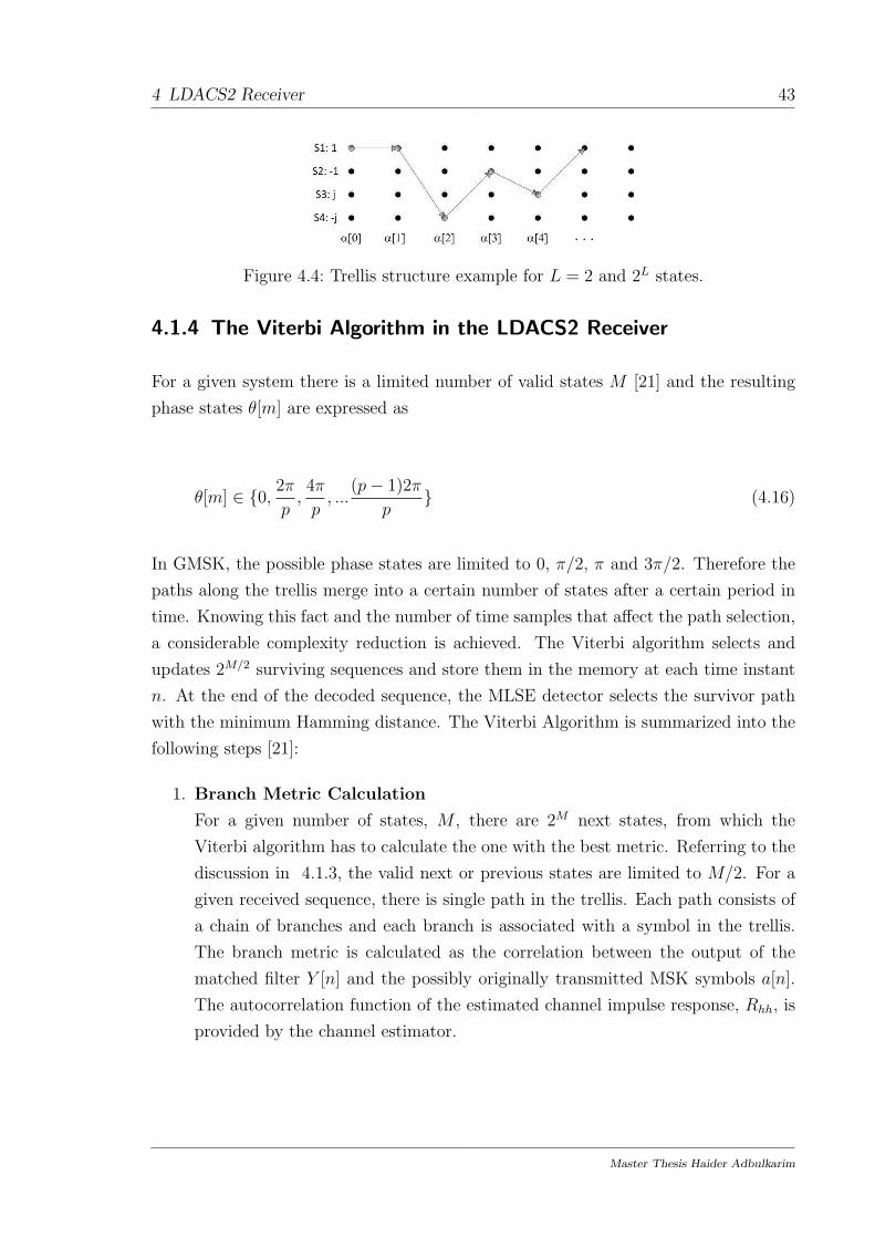
Figure 4.4: Trellis structure example for L = 2 and 2L states.

4.1.4 The Viterbi Algorithm in the LDACS2 Receiver

For a given system there is a limited number of valid states M [21] and the resulting

phase states θ[m] are expressed as

θ[m] ∈ {0, 2πp,4π

p, ...

(p− 1)2π

p} (4.16)

In GMSK, the possible phase states are limited to 0, π/2, π and 3π/2. Therefore the

paths along the trellis merge into a certain number of states after a certain period in

time. Knowing this fact and the number of time samples that affect the path selection,

a considerable complexity reduction is achieved. The Viterbi algorithm selects and

updates 2M/2 surviving sequences and store them in the memory at each time instant

n. At the end of the decoded sequence, the MLSE detector selects the survivor path

with the minimum Hamming distance. The Viterbi Algorithm is summarized into the

following steps [21]:

1. Branch Metric Calculation

For a given number of states, M , there are 2M next states, from which the

Viterbi algorithm has to calculate the one with the best metric. Referring to the

discussion in 4.1.3, the valid next or previous states are limited to M/2. For a

given received sequence, there is single path in the trellis. Each path consists of

a chain of branches and each branch is associated with a symbol in the trellis.

The branch metric is calculated as the correlation between the output of the

matched filter Y [n] and the possibly originally transmitted MSK symbols a[n].

The autocorrelation function of the estimated channel impulse response, Rhh, is

provided by the channel estimator.



The branch metric γ calculation is expressed as [10]

γ[n] = a∗[n]Rhh(0)a[n] + 2<{a∗[n]n−1∑

m=n−Lh

a[m]Rhh[n−m]}. (4.17)

Since a∗[n]a[n] = 1, the first term in (4.17) is fixed for all the branches and can

be omitted. Then (4.17) is simplified to

γ[n] = 2<{a∗[n]n−1∑

m=n−Lh

a[m]Rhh[n−m]}. (4.18)

2. Path Metric Calculation

According to Ungerboeck’s recursive form [20], the path metric ψ is calculated

as

ψ(Y [n]) = <{a∗[n]Y [n]} − γ[n]. (4.19)

3. Path Update

Since there are r possible branches leaving each state at time n, the selection of

the survival path is done by finding the path that maximizes (4.19). The number

of survival paths at the end of information sequence is equal to L.

4. Path Decision

The final step is simply choosing the path, amongM , that has the maximum path

metric ψ. In case that hard-decision is implemented, the output of the Viterbi

Equalizer is a[n], which is the sequence of symbols a long the selected trellis path.



a[n] is in the form of Non-Return-to-Zero (NRZ), is directly converted to RTZ

bits. Then the originally transmitted symbols x[n] are retrieved as

x[n] =a[n]

jx[n− 1]a[n− 1]. (4.20)

In case that soft-decision decoding is implemented, the output of the Viterbi

algorithm is not hard-limited to ±1, but rather quantized. It is found [21] that

a quantization level of 8 introduces a gain of about 2 dB in Eb/No compared

to hard-quantization. For instance, a Viterbi output level of +4 indicates high

confidence that the transmitted bit was 1 whereas +1 indicates less confidence.

For benefit, the soft-decision Viterbi output should be fed to the input of a

soft-convolutional decoder.

An important characteristic of GMSK Viterbi Equalizer is that a single error will

never occur (see discussion 6.2.7,[21]). That is, either double or burst bit errors will

occur. That is because even in the case of a single bit error, the survivor path will

never converge with the error-free path. This feature is exploited by converting double

errors into single errors, which is done by the differential encoding and decoding, at

the transmitter and receiver, respectively.

4.2 Mitigating Fading Channel Effects

When the ACs are overflying, maneuvering or taking off in rather crowded airports, the

experienced channel models are far from being pure AWGN (as described in Chapter

3). This section describes the techniques used to mitigate the fading channel effects.

Those techniques include channel coding and interleaving. For the sake of consistency,

they are discussed in the same context. Referring to Figure 4.5, one easily notices

the fading effect on the error performance of a communication system. In the case

of an AWGN channel (ideal channel), the effect of noise could be easily mitigated by

only increasing the Signal-to-Noise Ratio (SNR). On the other hand, for flat fading

channels within Rayleigh limit, i.e., no LOS components, the performance of the system

degrades severely. However, the bad performance of the system could be enhanced by



Figure 4.5: The good, the bad and the awful error performance [22].

increasing the SNR [22], even though this would be no feasible solution to increase it

beyond practical SNR values.

On the extreme case, which is though very common in Aeronautical Communication,

the frequency-selective fading or fast fading (ENR or TMA channel models) introduces

irreducible error rate performance. No matter how much the SNR is increased, the

error floor remains at high level and no possible communication could be established.

Fortunately, the performance can be enhanced using channel equalization techniques.

The MLSE equalizer described in 4.1.3 is a well known technique. By using the

appropriate coding type, error-floored BER curve could further be enhanced. The

BER after coding approaches the same AWGN performance for high efficiency codes.

In the next section a brief description of the FEC techniques is introduced.

4.2.1 Forward Error Correction

In wireless communication channels, FEC is an important part of the system, because

with a wise choice of the encoder at the transmitter side, the receiver is able to correctly



recover the transmitted data, even if errors have occurred. Generally, there are two

kinds of errors [22] occurring in the transmitted data:

1. Random errors: they tend to occur because of the thermal noise existing at the

front end of the receiver (generally approximated as AWGN).

2. Burst Errors: the errors in this case occur in a burst fashion (subsequent groups

of symbols are corrupted) due to the fading channel effects. Due to their depen-

dency, burst errors are said to have memory. This memory is equal to the the

fading channel length, Lh [23].

The random errors are efficiently mitigated by using some popular FEC codes. Convo-

lutional codes with maximum correcting capabilities [24] are mostly used to mitigate

random errors. Those codes are capable of correcting transmission errors, given that

the error pattern would not exceed the correcting capability of the coder, t. Where t

is defined as

t =dmin − 1

2(4.21)

Where dmin is defined as the smallest number of places (in bits) that any two code

words differ in the codebook. Obviously, codes with large dmin are a good choice.

Unfortunately, increasing the minimum distance also decreases the code rate Rc which

is defined as

Rc =k

n. (4.22)

Where k is the message length and n is the code word length. The other type of coders

are the block codes, which operate on a block basis rather than a bit basis. One of the

most popular coders is the Reed Solomon (RS) coder, which is a non binary cyclic coder

based on Galois Field (GF) area of mathematics. The notation RS(n, k,m) is often

used, where n is the total number of symbols in the encoded block, k is the number

of encoded data symbols and m is the symbol length, in bits. Taking RS(15, 11, 4) as

an example, this code can correct up to 2 symbols errors, each symbol of 4 bits. That



means a burst error of 8 bits can be corrected, given the error is exactly limited to 2

symbols.

It is always desirable to reduce the redundant bits as much as possible, i.e., increasing

the system throughput. Hence, there is a trade off between increasing code rate and

the number of errors that a coder can correct. Besides, decreasing Rc below a certain

limit will degrade the performance of the system, as seen in Figure 4.6 [25]. This

figure implies that the optimum RS code rate for a Gaussian channel is around 0.6.

On the other hand, for a Rician channel the optimal RS code rate is ranging from 0.4

to 0.6. The reason for the degradation of the BER performance at high Rc is, that the

less coding is applied to information bits, the more errors will occur.

The degradation at low Rc is more severe than that at high Rc. Two opposite mecha-

nisms at low Rc are observed: the first one is the increased coding redundancy, which

tries to mitigate errors. The second mechanism is the reduced energy per modula-

tion symbol (compared to the information bit energy), which results in more errors

in the demodulator. Finally, the second mechanism wins and thus the system error-

performance degrades.

Some techniques are used, however, to enhance the coders correction capability, keeping

Rc as high as possible, such as puncturing used in convolutional coding. However, Rc

cannot exceed a certain upper limit, as previously discussed.

To achieve a better performance in LDACS2, concatenated coding is considered, as

seen in Figure 4.7. With the suitable choice of coding parameters, concatenated

codes can achieve very high coding gains with efficient coding. The idea is simple:

the outer coder (usually a block coder) is responsible for correcting burst errors that

occurring from the convolutional coder while the inner coder (usually a convolutional

coder) corrects random errors. The random errors are non-correlated and related to

the AWGN.

The LDACS2 coding parameters are listed in Table 4.1.

4.2.2 Interleaving

Another useful technique is to use interleaving together with channel coding. The

interleaver function is simply spreading the bits (groups or individuals) within the

transmitted frame, after the coding block. The result is that correlated errors are



Figure 4.6: RS BER vs. code rate trade-off [25].

RS coderSymbol

interleaverSymbol to bit

Conv. coderBit interleaverRandomlyinterleavedcoded bits

Informationbits

RSsymbols

Interleavedsymbols

CC codedbits

Figure 4.7: Concatenated channel coding for LDACS2.

distributed among several code words, which leads to less errors per single code word.

This helps the coder to successfully correct the errors within its capability. There are

several types of interleavers described in the literature [24]. The Block interleaver,

recommended for LDACS2, makes the channel with memory L behave like a random

channel to the decoder. This results in less powerful codes are required to correct

transmission errors. At the transmitter, the block interleaver takes a block of bits

and writes them row-by-row fashion into a matrix and then reads the matrix into a



Table 4.1: LDACS2 coding parameters.

Parameter Value

Inner coder convolutional (7, 171, 133)Puncturing pattern [110101] for Rc = 3/4

Bit interleaver quasi randomOuter coder RS(15, 11, 4) or RS(31, 23, 5)

Outer interleaver symbol interleaverCoded BER 10−7 for uncoded BER of 10−3

column-wise fashion to feed the modulator. At the receiver, the operation is reversed.

The filling and reading the matrix introduces delays in the transmission chain.

The bit interleaver, on the other hand, is used after the convolutional coder to decor-

relate the AWGN effect and to randomize the bits within LDACS2 slot. The bit

interleaver, however, is simpler and there is no buffering delay introduced.

The use of both types of interleavers as well as the coders is intensively analyzed within

the LDACS2 against different aeronautical fading channels in Chapter 5.



5 LDACS2 Performance and Capacity

As stated in Chapter 1, the performance evaluation of LDACS2 is important in the

selection of the final LDACS proposal. In addition to AWGN, the system has to be

tested against the two main flying scenarios, those are the ENR and TMA channel

models.

In this chapter, the LDACS2 simulator is described in short. The simulation param-

eters are given. The system is then tested against the AWGN channel. Next, the

specified coding schemes are applied to the LDACS2 under the AGWN as well as ENR

and TMA channel models. More efficient code rates are proposed and tested under

the same conditions as well. The performance of the system is evaluated using the

BER as measure. The co-site interference from the DME interrogators is also studied.

Then, the system performance against time synchronization and frequency estimation

errors is investigated. Later, the system capacity is studied within the suggested spec-

ifications. Finally, the LDACS2 performance is compared to the LDACS1 within the

specified coding parameters.

5.1 LDACS2 Performance under Aeronautical Channel

Models

In this section, the LDACS2 simulator is described. However,the main transmitter and

receiver functions are described in detail in the Chapters 2 and 4 respectively.

5.1.1 LDACS2 Simulator

The LDACS2 simulator is built using the MATLAB simulation environment. The

MATLAB communications system toolbox is used. The outer coder, the symbol in-



terleaver, the inner coder, and the bit interleaver are built according to the LDACS2

specifications. The modulator and demodulator parts described in Chapters 2 and 4,

respectively, are partly adapted from the GSM simulator presented in the work [10].

However, the function implementation of the matched filter and the Viterbi algorithm

have been redefined according to the LDACS2 specifications to yield soft output. The

matched filter in LDACS2 should track the training sequence at the start of each burst,

taking into account the guard bits added and the message addresses, which is the main

difference from the GSM burst. The matched filter has also been redesigned to take ad-

vantage of the oversampled samples in the time domain for better channel estimation.

The aeronautical channel models are implemented in Java [27] programming language

and integrated into the MATLAB channel simulator code.

The framing structure of LDACS2 is analyzed and implemented for different slot

lengths, as seen in Section 1.3.3. The LDACS2 performance is tested first for the

specified specifications. Then, the specifications were modified and the performance is

tested again under the same channel models. Those adaptations include using stronger

codes, insertion of extra training sequences and longer burst structure. One of the

challenging tasks was to modify the matched filter according to the number of training

sequence.

The simulations are done using the Monte Carlo simulation method. The SNR is sim-

ulated in the range from 0 to 16 dB. For each value of SNR, 2 ·107 random information

bits are generated. This number of bits ensures a BER values of 1 ·10−6 to be obtained.

In each iteration, the BER ratio is calculated according to

BER =Ne

NT

, (5.1)

where Ne is the number of information bits decoded incorrectly, and NT is the total

number of information bits.

5.1.2 LDACS2 Performance in AWGN

As stated in Chapter 1, LDACS2 has different slot types. The main difference among

them is the length of each slot. This has an influence on the estimated channel impulse



response as well as the encoding-decoding implementation. In this section, the perfor-

mance of LDACS2 in the AWGN channel is simulated and compared to the theoretical

GMSK performance. Then, stronger codes are proposed and simulated.

The AWGN is a zero-mean complex Gaussian process, with a variance of σ2N of the

entire process. The AWGN is generated in the simulator according to

σ2N =

Fs

2

1

SNRl

, (5.2)

where Fs is the sampling rate, SNRl is the linear SNR, defined as

SNRl = 10(SNR10 ). (5.3)

The generated noise is then added to the original transmitted signal samples r[n] as

r[n] = x[n] + σN · z[n], (5.4)

where z is a function that generates normally distributed random values with a zero

mean and a variance of one.

To test the LDACS2 receiver, the estimated channel impulse response hrx is plotted

and compared to the Gaussian pulse shape at the transmitter 2.6. Figure 5.1 shows

that the estimated channel impulse response is approximately equivalent to the trans-

mitter pulse shaping function. However, is it slightly broadened due to the AWGN.

This means that the LDACS2 receiver can successfully estimate the channel impulse

response.



0 1 2 3 4 50

0.2

0.4

0.6

0.8

1

Tb

Am

pli

tude

Figure 5.1: Estimated channel impulse response at the channel estimator.

For the LDACS2 Down Link (DL), the CoS1 uncoded AWGN performance is simulated

and compared to the theoretical GMSK BER. The theoretical BER P can be calculated

by [32]

P = erfc(

√

β · Eb/N0

)

, (5.5)

where:

β: is a factor related to BT product. For BT = 0.3, β is 0.89,

Eb/N0 is the energy per bit.

Figure 5.2 shows that the LDACS2 uncoded BER performance is close to the the-

oretical GMSK BER performance. However, the theoretical BER does not consider

the transmission channel impulse response, while the simulated BER assumes the ex-

istence of the transmission channel and estimates the channel impulse response hrx

accordingly (as defined Section 4.1.1). Hence the degradation in the simulated BER

in comparison to the theoretical BER. On the other hand, the simulated BER matches

the LDACS2 specifications [2].

Next, the specifications coding is simulated in the AGWN channel. In the practical

implementation of LDACS2, the data bits are encoded. With coding, the information

bit rate Ri is inversely proportional to Rc. Referring to the CoS1 slot structure in

Figure 1.9, the information part is 144 bits and the FEC part is only 49 bits. Besides,



0 2 4 6 8 10 12 14 1610

−6

10−5

10−4

10−3

10−2

10−1

100

Eb/N

0

BE

R

Theoretical

Simulated

Figure 5.2: CoS1: non-coded AWGN.

0 2 4 6 8 10 12 14 1610

−6

10−5

10−4

10−3

10−2

10−1

100

SNR

BE

R

No cod

RS(15,11,4)+CC(3/4)

CC(3/4)

Figure 5.3: CoS1: coded AWGN, specifications coding.

only short code words, that can fit in the 193 bit-duration, can be used. Therefore,

only RS code with (15, 11, 4) concatenated with CC of L = 7 are considered.

Figure 5.3 shows the performance of both concatenated coding and single code.

It is obvious that when using concatenated coding, no performance improvement is

achieved. This is because the RS(15, 11, 4) introduces no further enhancement on the



0 2 4 6 8 10 12 14 1610

−6

10−5

10−4

10−3

10−2

10−1

100

SNR

BE

R

No cod

RS(15,11,4)+CC(1/2)

CC(1/2)

Figure 5.4: CoS1: coded AWGN (proposed coding).

error correction, since the slot length is short. This performance does not comply

with the LDACS2 specification, which require a coded BER of 10−7 for an uncoded

BER of 10−3. Therefore, stronger coding is proposed. By using the same RS(15, 11, 4)

but with CC(1/2), the curves shown in Figure 5.4 are obtained. There is a gain in

the performance of about 4 dB compared to CC(3/4). Again, a CC with (Rc = 1/2)

performs the same as the concatenated coding.

The CoS2 slot performance in the coded AWGN using the specification coding is

considered next. The CoS2 slot length is 1806 bits, which is equivalent to 6.66 ms.

The user data part is 1304 bits and the FEC part is 394 bits (see Figure 1.10). The

performance of CoS2 in the coded AWGN channel using the recommendation coding

is shown in Figure 5.5. Since the CoS2 slot is longer than CoS1, longer code is used.

Hence, RS(31, 23, 5) concatenated with CC(3/4) are used. It can bee seen that the

performance of concatenated coding for the CoS2 slot is better than a CC(3/4).

It is also possible to have a CoS2 burst, containing longer messages and spanning

multiple CoS2 slots (as mentioned in Chapter 1). The AWGN performance of a CoS2

burst spanning 10 CoS2 slots is shown in Figure 5.6. Compared to a single slot, the

BER of a CoS2 burst has a performance gain of about 2 dB using the same coding.

This is due to the fact that the RS symbol interleaver can spread adjacent symbols

over multiple RS codewords and thus less errors occur per single RS code word.



0 2 4 6 8 10 12 14 1610

−6

10−5

10−4

10−3

10−2

10−1

100

SNR

BE

R

No cod

RS(31,23,5) + CC(3/4)

CC(3/4)

Figure 5.5: CoS2 slot: coded AWGN (specifications coding).

0 2 4 6 8 10 12 14 1610

−6

10−5

10−4

10−3

10−2

10−1

100

SNR

BE

R

No code

RS(31,23,5) + CC(3/4)

CC(3/4)

Figure 5.6: CoS2 burst: coded AWGN (specifications coding).

The LDACS2 Up Link (UL) performance is shown in Figure 5.7 for a UP burst of

length 13.3 ms. From this figure, it can be inferred that the performance of a UP burst

is similar to that of a CoS2 single slot.



0 2 4 6 8 10 12 14 1610

−6

10−5

10−4

10−3

10−2

10−1

100

SNR

BE

R

No cod

RS(31,23,5)+CC(3/4)

Figure 5.7: UP burst: coded AWGN (specifications coding).

It should be mentioned that the BER performance for the CoS2 slot, burst and UP

burst can also be enhanced by using CC(1/2) concatenated with RS(31, 23, 5), as shown

in Figure 5.4.

5.1.3 LDACS2 Performance in ENR Channel

In this section, the LDACS2 performance in the ENR channel model is simulated. As

mentioned in Chapter 3, the ENR channel model has two taps, the first is the LOS

echo while the other is the off-path echo. The ENR channel power delay profile is

shown in Figure 5.8.

For the simulations, perfect time and frequency synchronization are assumed. The

CoS1 slot performance within ENR is shown in Figure 5.9. In this figure, both the

specified and the proposed coding are simulated. It is obvious that the specified coding

RS(15, 11, 4) + CC(3/4) does not introduce a considerable coding gain compared to

the uncoded curve. However, by using the proposed stronger CC of rate (1/2), the

performance of a CoS1 slot approaches the recommended BER of 10−7. Similarly to

the AWGN, for short slot lengths, CC has the same performance as the concatenated

coding.



0 2 4 6 8 10 12 14 16 18 20−40

−30

−20

−10

0

τ [µs]

Rel

ativ

e pow

er, dB

Figure 5.8: ENR channel power delay profile.

0 2 4 6 8 10 12 14 1610

−6

10−5

10−4

10−3

10−2

10−1

100

SNR

BE

R

No cod

RS(15,11,4)+CC(3/4)

RS(15,11,4)+CC(1/2)

CC(1/2)

CC(3/4)

Figure 5.9: CoS1 slot: coded ENR, specifications vs. proposed coding.

The specified and proposed coding for the CoS2 slot under the ENR channel are

simulated next. Figure 5.10 shows the bad performance of the specified concatenated

coding RS(31, 23, 5) and CC(3/4). Even when using the proposed stronger CC of rate

(1/2), there is an error floor of BER = 10−5. Because there is one training sequence for

each CoS2 slot, the estimated channel impulse response hrx is not valid for the entire

6.66 ms duration of the CoS2 slot, and thus the severe degradation in performance is

observed.



0 2 4 6 8 10 12 14 1610

−6

10−5

10−4

10−3

10−2

10−1

100

SNR

BE

R

No cod

RS(31,23,5) + CC(3/4)

RS(31,23,5) + CC(1/2)

CC(3/4)

Figure 5.10: CoS2 slot: coded ENR, specifications vs. proposed coding.

To overcome this degradation, the CoS2 burst structure is next considered. However,

the LDACS2 specification defines the usage of only one training sequence for either a

slot or a burst, regardless of their lengths. Considering a normal GSM burst of 0.5 ms,

there is one training sequence per each burst. Since the LDACS2 channel estimation

and equalization is similar to the GSM except for the slot length, an adaptation is

proposed to the burst structure. Considering a CoS2 burst of length 66.6 ms, this

burst is 133 times the length of a GSM burst. Hence it is suggested to insert one

training sequence for each 6.66 ms part of a CoS2 burst. Thus, for a CoS2 burst of

66.6 ms, 10 training sequences are inserted. Thus the estimated channel is only used

for each 6.66 ms part of the entire burst. This approach is implemented in the rest of

the simulations, whenever a burst structure is simulated.

The performance of a CoS2 burst of 66.6 ms length is shown in Figure 5.11. Both

the specified and the proposed coding are simulated under the ENR channel. Due to

the longer length of the burst, the RS symbol interleaver can interleave the adjacent

symbols over multiple RS codewords. Thus, a burst error will not affect two adjacent

codewords and hence a considerable performance enhancement is observed. Using the

proposed CC of rate (1/2) concatenated with RS(31, 23, 5), there is a gain of about 6

dB compared to the specified coding.

The influence of the CoS2 burst length and the BER performance using the specified

coding is shown in Figure 5.12. Obviously, as the burst length increases, higher coding



0 2 4 6 8 10 12 14 1610

−6

10−5

10−4

10−3

10−2

10−1

100

SNR

BE

R

No cod

RS(31,23,5)+CC(3/4)

RS(31,23,5)+CC(1/2)

Figure 5.11: CoS2 burst: coded ENR, specifications vs. proposed coding.

0 2 4 6 8 10 12 14 1610

−6

10−5

10−4

10−3

10−2

10−1

100

SNR

BE

R

1 slot

2 slot

5 slot

10 slot

Figure 5.12: CoS2 burst size influence, ENR, specified coding: RS(31, 23, 5) +CC(3/4).

gain can be achieved. Using the proposed coding of CC(1/2) for the same burst size

and the same ENR channel, further performance improvement is achieved, as seen in

Figure 5.13.



0 2 4 6 8 10 12 14 1610

−6

10−5

10−4

10−3

10−2

10−1

100

SNR

BE

R

1 slot

2 slot

5 slot

10 slot

Figure 5.13: CoS2 burst size influence, ENR, proposed coding: RS(31, 23, 5) +CC(1/2).

The UP burst performance in coded ENR is depicted in Figure 5.14. Similar to the

coded AWGN, the performance of a UP burst of length 13.3 ms with single training

sequence per burst resembles the performance of a single CoS2 slot in the ENR channel.

This is because of the similar structure of both of the CoS2 and UP bursts for the same

burst length.

This work proposes another possibility to enhance the system performance in the ENR

channel is to introduce more training sequences per a single slot. This makes hrx valid

only for part of the slot and then a new hrx is estimated for the next part. The effect

of increasing the number of training sequences per the slot is shown in Figure 5.15.

Although it enhances the performances significantly, it reduces the system capacity by

introducing extra redundant bits into the slot. The same discussion applies to the UP

burst but it is not simulated due to its similarity with CoS2 slot.

5.1.4 LDACS2 Performance in the the TMA Channel

The TMA channel model is different from ENR in that it has less Doppler shift due

to lower speed of the AC. The maximum experienced Doppler shift is 500 Hz. How-

ever, the TMA power delay profile follows an exponential decay (Figure 5.16), which



0 2 4 6 8 10 12 14 1610

−6

10−5

10−4

10−3

10−2

10−1

100

SNR

BE

R

No cod

RS(23,31) + CC(3/4)

RS(23,31) + CC(1/2)

Figure 5.14: UP burst: coded ENR, specifications vs proposed coding.

0 2 4 6 8 10 12 14 1610

−6

10−5

10−4

10−3

10−2

10−1

100

SNR

BE

R

1 TR

3 TR

6 TR

Figure 5.15: Number of training sequences per a single CoS2 slot, ENR, specified cod-ing: RS(31, 23, 5) + CC(3/4).

indicates that the LDACS2 performance suffers more degredation in the TMA channel

than in the ENR channel. The CoS1 slot performance under the TMA channel using

the specification coding of CC(3/4) is shown in Figure 5.17. Since the burst errors

are beyond the capability of the coder, the decoder decodes the codewords wrongly,

and thus the performance is worst than the non-coded case. Even with the proposed



1 2 3 4 5 6 7 8 9 10−30

−20

−10

0

τ [µs]

Rel

ativ

e pow

er, dB

Figure 5.16: TMA channel power delay profile.

0 2 4 6 8 10 12 14 1610

−3

10−2

10−1

100

SNR

BE

R

No cod

RS(15,11,4)+CC(1/2)

CC(1/2)

CC(3/4)

Figure 5.17: CoS1 slot: coded TMA, specifications vs. proposed coding.

strong coding of CC(1/2), there is an error floor of BER = 10−2. CoS2 slots and UP

burst show similar performance in the TMA channel.

Considering the CoS2 burst structure of 66.6 ms using the specified coding of RS(31, 23, 5)

with a CC(3/4), the performance is very poor and is comparable to the non-coded case,

as shown in Figure 5.18. However, using the proposed coding of RS(31, 23, 5) with a

CC(1/2), the performance significantly enhances, as shown is the same figure.

In addition to the burst structure, increasing the the number of training sequences will

also enhance the performance, as seen in Figure 5.15.



0 2 4 6 8 10 12 14 1610

−6

10−5

10−4

10−3

10−2

10−1

100

SNR

BE

R

No cod

RS(31,23,5)+CC(3/4)

RS(31,23,5)+CC(1/2)

Figure 5.18: CoS2 burst: TMA, specifications vs. proposed coding.

5.1.5 DME Co-site Interference

In this section, the performance of LDACS2 against co-site interference from a DME

interrogator is evaluated. A UP burst of length 66.6 ms is chosen and an AWGN

channel is assumed. One training sequence is inserted every 6.66 ms. The LDACS2

receiver is assumed to receive data from the LDACS2 GS while a DME interrogator

sends pulses at a rate of 150 Pulse Pairs Per Second (ppps). To mitigate the co-site

interference, the LDACS2 receiver is assumed to blank its received signal whenever

high power pulses are detected. This approach is known as pulse blanking. At a rate

of 150 PPPS, a maximum of one DME pulse is expected to occur every 6.66 ms, i.e., 10

DME pulses within the simulated UP burst. Each DME pulse pair has a duration of

approximately 17µs, which is equivalent to 5 bits of the received data is to be blanked.

The LDACS2 receiver performance against DME co-site interference is shown in Figure

5.19. The LDACS2 performance hardly degrades due to the DME interference. This is

an important feature of LDACS2 in that it is possible to deploy LDACS2 while DME

interrogators are in service.



0 2 4 6 8 10 12 14 1610

−6

10−5

10−4

10−3

10−2

10−1

100

SNR

BE

R

1 pp

2 pp

3 pp

4 pp

5 pp

10 pp

Figure 5.19: UP burst performance against co-site DME, AWGN, specified coding:RS(31, 23, 5) + CC(3/4).

5.1.6 Time and Frequency Error Performance

In this section, the LDACS2 robustness against time synchronization errors as well as

frequency estimation errors are tested. Synchronization errors are assumed to occur

whenever the start of the burst (UL or DL) is shifted in time. Although the LDACS2

specification assumes a very accurate synchronization, errors have to be tested. For

this reason, a CoS2 burst is considered and ENR channel is assumed. The SNR is kept

fixed at 10 dB and the synchronization error is introduced in time to the input of the

channel estimator as a Gaussian process with zero mean and a standard deviation σ∆t

defined as

σ∆t = σt · Tb, (5.6)

where σt is the standard deviation of the error. σ∆t is then rounded to the nearest

integer and added to the value k that represents the actual start of the burst, as

calculated in (4.10).



0 1 2 3 4 5 610

−6

10−5

10−4

10−3

10−2

10−1

σ∆t

[Tb]

BE

R

Figure 5.20: CoS2 burst performance against synchronization error, AWGN, SNR =10 dB, specified coding: RS(31, 23, 5) + CC(3/4).

The simulation results are shown in Figure 5.20. Since the channel estimator tracks

the starting of the burst (as seen in Chapter 4), the simulation curves show acceptable

performance of the system up to an error variance of 3Tb. In reality, the synchronization

error occur infrequently because the LDACS2 GS forces the AC to stay in synchro-

nization on a timely basis (similar to the GSM where the synchronization burst is

defined).

LDACS2 robustness against frequency estimation error is also tested. To estimate the

exact carrier frequency Fc, fD should be exactly known at the receiver to compensate

for the shift in Fc. The error in fD estimation leads to an error in Fc synchronization.

The standard deviation of the error introduced in the frequency estimation σ∆f is

defined as

σ∆f = σf · Fc, (5.7)

where σf is the standard deviation of the error. After generating σ∆f , it is added to

fD in the receiver to simulate the error in the frequency estimation. The system per-

formance is shown in Figure 5.21. Unlike time synchronization error, LDACS2 shows

high sensitivity to errors in frequency estimation. An error in frequency estimation



0 5 10 15 20 2510

−6

10−5

10−4

10−3

10−2

10−1

100

σ∆f

[Hz]

BE

R

Figure 5.21: CoS2 burst performance against Frequency error, ENR channel, SNR =10 dB, specified coding: RS(31, 23, 5) + CC(3/4).

of 15 Hz degrades the BER to 10−1. Thus very accurate frequency synchronization

algorithms are required at the LDACS2 receiver.

5.2 LDACS2 Capacity

In this section, the LDACS2 capacity is analyzed. A typical LDACS2 frame is con-

sidered and the UL and DL information bit rates Ri are calculated. In addition, the

effect of inserting extra training sequence per a slot on the information bit rate is

investigated.

As known, the gross bit rate Rb, defined in Chapter 1, is different from the actual

information rate Ri. Rb is defined as the rate at which all the bits in the slot are

transmitted per second, including redundant bits and guard bits. Obviously, Ri is

smaller than Rb because there are always redundant bits to be added. To evaluate

the LDACS2 capacity in terms of Ri, a high density cell is considered. The scenario

assumes the existence of 204 AC per cell, which is the maximum number of ACs to be

supported by LDACS2. The length of each section and the according number of slots

are given in Table 5.1.



According to this configuration, the offered Ri will vary according to Rc, burst length

(UP and CoS2) and the number of training sequence per burst. Table 5.2 summarizes

the UL and DL information rate for different parameters.

Table 5.1: High density LDACS2 scenario

Section Slot/section Slot length (bits)

UP1 14 3612CoS1 204 300LoG2 4 902UP2 14 3612CoS2 58 1806

Table 5.2: LDACS2 capacity example

LDACS2 Coding Slot/burst Ri [kbps]

Overall CC(3/4) 1 115.2UL CC(3/4) 1 35.3DL CC(3/4) 1 80

Overall CC(1/2) 1 73.1UL CC(1/2) 1 22.4DL CC(1/2) 1 59

Overall CC(3/4) 2 108.7UL CC(3/4) 2 29DL CC(3/4) 2 79.7

Overall CC(3/4) 5 107.1UL CC(3/4) 5 24.6DL CC(3/4) 5 82.5

Overall CC(3/4) 10 107.9UL CC(3/4) 10 25.6DL CC(3/4) 10 82.3

It can be seen that using the moderate CC(3/4) coding, the overall Ri is 115 kbps for

both the UL and DL. A comprise between the UL and DL information rates could be

achieved by modifying the length of UL and DL section to cope with different traffic

requirements. However, this code rate is seen to perform badly in aeronautical channels

and hence when using a stronger CC of rate (1/2), the overall LDACS2 capacity drops

to 73 kbps. Another option is to transmit data in bursts spanning multiple slots (for

CoS2 and UP sections only). It is noted that, increasing the burst size to 5 enhances

the capacity as well as the performance (as seen in Section 5.1.3). Even increasing

the burst size to 10 slots will maintain the same information rate but enhances the



Figure 5.22: LDACS1 FL structure, one OFDM symbol in frequency domain [33].

performance further. One training sequence has been inserted for each slot to enhance

the performance. However, it should be mentioned that when using a burst structure,

the number of users that can simultaneously access those bursts decreases significantly.

On the other hand, for all scenarios, the number of users that can access the CoS1

section remains unchanged and thus critical messages are guaranteed to be exchanged

at the same rate.

5.3 LDACS2 vs. LDACS1 Performance

In this section, the LDACS1 is described in summary. The main physical parameters

are illustrated as well as the channel coding and modulation. Then, performance

comparision between the LDACA1 and LDACS2 is carried out.

5.3.1 LDACS1 Parameters

The LDACS1 physical layer is an OFDM-based modulation, designed to operate in

the L-band. The LDACS1 FL is a continuous OFDM transmission, while the LDACS1

RL is based on OFDMA-TDMA. This allows different users to access the burst on

demand. The LDACS1 FL transmission description is shown in Figure 5.22. It can be

seen that guard times are used on both sides of the spectrum, to prevent out-of-band

radiation. The LDACS1 RL transmission structure is shown in Figure 5.23. Each

user has its assigned time slot and sub-carrier. The time-frequency structure is called

tile. Table 5.3 summaries the main parameters used both in the FL and RL.

The LDACS1 has the same concatenated coding schemes, i.e., the outer coder is RS

and the inner coder is CC. The FL frame of 2184 bits is coded with RS(101, 91, 5) con-

catenated with CC(1/2). The RL data segment of 672 bits is coded with RS(98, 84, 7)

concatenated with CC(1/2). The encoded bits, together with redundancy, headers and



Figure 5.23: LDACS1 RL structure [33].

Table 5.3: LDACS1 OFDM parameters

Parameter Value

FFT size 64Sampling time 1.6 µs

Sub-carrier spacing 9.76 kHzUseful symbol time 102.4 µsOFDM symbol time 120 µs

Lower frequency guard sub-carriers 7Higher frequency guard sub-carriers 6

FL structure frameRL structure tileFL capacity 2442 bits/frameRL capacity 134 symbols/tile

Figure 5.24: LDACS1 super frame [33].

trailers are formed into a Super-Frame (SF) structure. Each SF is 240 ms and corre-

sponds to 2000 OFDM symbols. The SF is shown in Figure 5.24. Finally, each frame

is then modulated.The LDACS1 supports Gray-mapped QPSK, 16QAM and 64QAM.



5.3.2 Performance Comparison

In this section, a comparison between LDACS1 and LDACS2 is carried out. The

LDACS1 is an OFDM-based system, which has an effective channel bandwidth of 500

kHz. For a fair comparison between both systems, the received power Pr is assumed

to be equal for both, LDACS1 and LDACS2. The linear SNR is defined as [28]

SNRl =Pr

N0B, (5.8)

where B is the bandwidth of the baseband signal and N0B is the total noise power

within the passband signal bandwidth 2B. Then for LDACS1, the SNRl is written as

SNRl1 =Pr

N0 · 500 kHz. (5.9)

The SNRl for LDACS2 is written as

SNRl2 =Pr

N0 · 200 kHz. (5.10)

Then the relationship is

SNRl2 = 2.5 · SNRl1, (5.11)

and in the logarithmic dB scale, the relationship is written as

SNR2 = 4 + SNR1. (5.12)



0 2 4 6 8 10 12 14 1610

−6

10−5

10−4

10−3

10−2

10−1

100

Eb/N

o

BE

R

LDACS1 FL data

LDACS2 UP, RS(31,23,5)+CC(3/4)

LDACS2 UP, RS(31,23,5)+CC(1/2)

Figure 5.25: LDACS1 FL data frame, RS(101, 91, 5) + CC(1/2) vs. LDACS2 UP burst(specifications vs. proposed coding).

(5.12) shows that the SNR of LDACS2 is larger than that of LDACS1 by 4 dB, due

to the smaller bandwidth of LDACS2 compared to LDACS1.

To compare both LDACS1 and LDACS2, Eb/N0 in logarithmic scale (dB) is used

instead of the SNR. The relation between (Eb/N0) dB and the SNR is given by

(Eb/N0) dB = SNR− 10 logRc. (5.13)

The LDACS1 Forward-Link (FL) data frame [33], which has 2184 information bits

and the LDACS2 UP burst are simulated and compared in Figure 5.25 for the ENR

channel.

Clearly, the LDACS1 performance is better than LDACS2 for the UL, using the

specification coding. This is due to the stronger coding of LDACS1 compared to

LDACS2. Besides, the LDACS1 frame has several pilot symbols distributed over time

and frequency, which makes the channel estimation more accurate in fast fading chan-

nels. Even with the proposed stronger coding, LDACS1 performance still better than

LDACS2.



The performance of an LDACS1 Reverse-Link (RL) data segment of 672 information

bits is next compared to the LDACS2 CoS2 slot in Figure 5.26. The performance of

LDACS1 RL is also better than that of LDACS2 DL, even with the proposed stronger

coding.

0 2 4 6 8 10 12 14 1610

−6

10−5

10−4

10−3

10−2

10−1

100

Eb/N

o

BE

R

LDACS1 RL data

LDACS2 CoS2, RS(31,23,5)+CC(3/4)

LDACS2 CoS2, RS(31,23,5)+CC(1/2)

Figure 5.26: LDACS1 RL data segment, RS(98, 84, 7) + CC(1/2) vs. LDACS2 CoS2slot (specifications vs. proposed coding).


6 Conclusions 75

6 Conclusions

In this master thesis, the LDACS2 proposal is studied. The LDACS2 model is imple-

mented in a software simulator. Its performance is evaluated for the first time and

important results are obtained. Those results can be used in the final selection of one

of the two proposals for the future aeronautical communication system.

6.1 Implementaion

One of the main tasks of this work is the analysis of the LDACS2 proposal specifica-

tions. Since the LDACS2 transmitter and receiver parameters are not mentioned in

the specifications, they are first investigated and determined. Due to its basic princi-

ple as a GMSK transmission concept, the LDACS2 transmitter is built similar to the

GSM specifications. Then, channel coding, multiplexing and modulation are imple-

mented, tested and verified according to the LDACS2 frame structure. The LDACS2

receiver is then implemented. Successful demodulation is achieved by using channel

equalization algorithm known from the GSM. The LDACS2 receiver is also tested for

the correct demodulation of the received signal waveform. The channel decoding is

also implemented and tested.

Adapting the aeronautical channel models as described in [27] is the next important

task of this thesis. The channel model implementation is adapted to fit the TDMA

environment of the LDACS2.

The other accomplished task is simulating the LDACS2 within the aeronautical channel

models environments. The simulations are done using the MATLAB simulator. Taking

into account the long LDACS2 burst compared to the GSM, many implementation

techniques have to be done to cope with time synchronization, channel estimation

and channel equalization. Since the GSM specification supports low speed mobility,


6 Conclusions 76

the great challenge was to adapt channel equalization to cope with very high speeds

experienced in aeronautics environments.

Further enhancements on the system are proposed and validated through simulations.

Those include the insertion of extra training sequences, a longer burst structure and

stronger coding.

6.2 Results

The simulation results of LDACS2 show the plausibility of the system deployment.

The LDACS2 performance using the specified code rate and slot structure showed a

poor performance. However, considerable enhancements on the system performance

are proven using stronger coding with the same slot structure. However, with stronger

codes, the information bit rates are decreased. On the other hand, introducing more

training sequences per single burst while maintaining the specified code rate achieves

the same performance, as shown by the simulation results.

A third possibility is to transmit the data in bursts spanning multiple slots instead of

single slot. This has the advantage of encoding longer messages and then the symbols

are interleaved further apart across the burst, which minimizes the effect of burst errors.

It has been shown that a burst of up to 5 basis slots with the specified CC with Rc = 3/4

performs the same as single slot structure with stronger CC with Rc = 1/2. Thus,

the information bit rate is kept at maximum while keeping the system performance at

acceptable level.

The simulation results also showed that for short-length slots, such as CoS1 slots, it

is sufficient to use only CC instead of concatenated codes (RS with CC). Simulations

showed that there is no coding gain when using concatenated codes compared to single

code.

The simulations also show that the LDACS2 is robust against time synchronization

errors that occur at the receiver. The system shows an acceptable performance.

However, the simulations showed that the LDACS2 is less robust against errors in

frequency estimation.


6 Conclusions 77

The overall information rate, however, is low compared to nowadays offered bit rates.

As illustrated in the implementation example, for a cell with a maximum capacity of

204 AC, the offered bit rate cannot exceed 115 kbps for both the UL and DL. This

shows that the LDACS2 system support basic data communications, like navigation

and traffic control. There is even the possibility of supporting voice using the existing

structure or a separate voice channel. However, to increase the offered information

rate, many solutions on the system are to be introduced. One of those is to aggregate

channels to have higher information data rates, as suggested in the specifications.

6.3 Design Drawbacks

Since the LDACS2 slot relies on the training sequence to estimate the channel, the

currently specified training sequence position is not practical. To be able to estimate

the accurate channel impulse response, the training sequence should be placed in the

middle of the slot, similarly to the GSM. Besides, long slots (CoS2 and UP) have bad

performance because of the single trainging sequence dedicated to the entire slot. This

leads to bad performance for fast fading channels, as seen in Section 5.1.3.

Another design drawback is the location of the CRC, which is outside the coded data.

For the receiver to be able to determine transmission errors that pass the FEC coding,

the CRC should also be protected by coding. Thus, it is recommended that the CRC

is coded together with the user data.

The LDACS2 proposal is a half-duplex system. To increase the offered Ri, full-duplex

implementation is recommended for simultaneous access of both the AC and the GS.

This requires channel aggregation among at least two channels. The full-duplex system

will then offer higher data rates according to the number of aggregated channels.

6.4 Future Work

Further enhancements could be introduced into the LDACS2 to increase its information

rate. General Packet Radio Service (GPRS), High-Speed Downlink Packet Access

(HSDPA) and Enhanced Data rates for GSM Evolution (EDGE) data services used

in the GSM can be applied. The 8PSK modulation scheme applied in the EDGE, for


6 Conclusions 78

example, can be implemented on the top of the existing single carrier modulation in

LDACS2, providing higher bit rates than that of the GMSK modulation. The frame

structure, however, needs to be adapted according to the implemented services.

To enhance the LDACS2 BER performance against aeronautical channels, the usage

of more efficient codes is suggested. Turbo-codes [34] are recommended. Those codes

perform better and less sensitive to puncturing than the convolutional codes. They

approach the Shannon limit for channel capacity and thus will increase the offered Ri.

However, Turbo-codes are not suitable for short length slots, like the CoS1 slot. Block

codes can also be implemented. However, there is a trade-off between their reliability

against channel impairments and their complexity. Hybrid Automatic Repeat Request

(hybrid ARQ) is also another potential to enhance the LDACS2 performance against

errors. The principle is to send the redundancy bits only when the message is detected

as corrupted by the CRC. However, the trade-off of this technique is lower system

throughput. Validating the performance of those codes and techniques is then through

simulations is necessary before deployment.


Acronyms 79

Acronyms

LDACS1 L-band Digital Aeronautical Communications System, Type1 . . . . . . . . . . . . 1

LDACS2 L-band Digital Aeronautical Communications System, Type2 . . . . . . . . . . . . 1

AWGN Additive White Gaussian Noise . . . . . . . . . . . . . . . . . . . . . . . . . . . . . . . . . . . . . . . . . . . .1

FCS Future Communication Study . . . . . . . . . . . . . . . . . . . . . . . . . . . . . . . . . . . . . . . . . . . . . . . . 1

ICAO International Civil Aviation Organization . . . . . . . . . . . . . . . . . . . . . . . . . . . . . . . . . . . 1

MAC Medium Access Control . . . . . . . . . . . . . . . . . . . . . . . . . . . . . . . . . . . . . . . . . . . . . . . . . . . . . 1

BER Bit Error Rate . . . . . . . . . . . . . . . . . . . . . . . . . . . . . . . . . . . . . . . . . . . . . . . . . . . . . . . . . . . . . . . 1

ARS Aeronautical Radio-navigation Services . . . . . . . . . . . . . . . . . . . . . . . . . . . . . . . . . . . . . . 2

FDMA Frequency Division Multiple Acces . . . . . . . . . . . . . . . . . . . . . . . . . . . . . . . . . . . . . . . . 2

TDMA Time Division Multiple Access . . . . . . . . . . . . . . . . . . . . . . . . . . . . . . . . . . . . . . . . . . . . 2

AMACS All Purpose Multichannel Aviation Communication System . . . . . . . . . . . . . . 2


Acronyms 80

ATC Air Traffic Control . . . . . . . . . . . . . . . . . . . . . . . . . . . . . . . . . . . . . . . . . . . . . . . . . . . . . . . . . . . 4

AOC Airline Operational Control. . . . . . . . . . . . . . . . . . . . . . . . . . . . . . . . . . . . . . . . . . . . . . . . . .4

DLS Data Link Sublayer . . . . . . . . . . . . . . . . . . . . . . . . . . . . . . . . . . . . . . . . . . . . . . . . . . . . . . . . . . 5

LSS LDACS2 Service Sublayer . . . . . . . . . . . . . . . . . . . . . . . . . . . . . . . . . . . . . . . . . . . . . . . . . . . . 5

LME Link Management Entity . . . . . . . . . . . . . . . . . . . . . . . . . . . . . . . . . . . . . . . . . . . . . . . . . . . . 6

LML Link Management Layer . . . . . . . . . . . . . . . . . . . . . . . . . . . . . . . . . . . . . . . . . . . . . . . . . . . . . 6

TDD Time Division Duplexing . . . . . . . . . . . . . . . . . . . . . . . . . . . . . . . . . . . . . . . . . . . . . . . . . . . . 6

LDL L-band Digital Link . . . . . . . . . . . . . . . . . . . . . . . . . . . . . . . . . . . . . . . . . . . . . . . . . . . . . . . . . . 7

VDL VHF Digital Link. . . . . . . . . . . . . . . . . . . . . . . . . . . . . . . . . . . . . . . . . . . . . . . . . . . . . . . . . . . .7

GMSK Gaussian Minimum Shift Keying . . . . . . . . . . . . . . . . . . . . . . . . . . . . . . . . . . . . . . . . . . 7

MSK Minimum Shift Keying . . . . . . . . . . . . . . . . . . . . . . . . . . . . . . . . . . . . . . . . . . . . . . . . . . . . . . 7

QPSK Quadrature Phase Shift Keying . . . . . . . . . . . . . . . . . . . . . . . . . . . . . . . . . . . . . . . . . . . . 7

FSK Frequency Shift Keying . . . . . . . . . . . . . . . . . . . . . . . . . . . . . . . . . . . . . . . . . . . . . . . . . . . . . . 8

ISI Inter Symbol Interference . . . . . . . . . . . . . . . . . . . . . . . . . . . . . . . . . . . . . . . . . . . . . . . . . . . . . . 9


Acronyms 81

NM Nautical Mile . . . . . . . . . . . . . . . . . . . . . . . . . . . . . . . . . . . . . . . . . . . . . . . . . . . . . . . . . . . . . . . . .9

AC Aircraft . . . . . . . . . . . . . . . . . . . . . . . . . . . . . . . . . . . . . . . . . . . . . . . . . . . . . . . . . . . . . . . . . . . . . . 10

GS Ground Station . . . . . . . . . . . . . . . . . . . . . . . . . . . . . . . . . . . . . . . . . . . . . . . . . . . . . . . . . . . . . . 10

RS Reed Solomon . . . . . . . . . . . . . . . . . . . . . . . . . . . . . . . . . . . . . . . . . . . . . . . . . . . . . . . . . . . . . . . . 17

CRC Code Redundancy Check . . . . . . . . . . . . . . . . . . . . . . . . . . . . . . . . . . . . . . . . . . . . . . . . . . . 17

RTZ Return-to-Zero . . . . . . . . . . . . . . . . . . . . . . . . . . . . . . . . . . . . . . . . . . . . . . . . . . . . . . . . . . . . . 20

MLSE Maximum Likelihood Sequence Estimator . . . . . . . . . . . . . . . . . . . . . . . . . . . . . . . . . 23

PSD Power Spectrum Density. . . . . . . . . . . . . . . . . . . . . . . . . . . . . . . . . . . . . . . . . . . . . . . . . . . .25

LOS Line of Sight . . . . . . . . . . . . . . . . . . . . . . . . . . . . . . . . . . . . . . . . . . . . . . . . . . . . . . . . . . . . . . . . 27

ACF Autocorrelation Function . . . . . . . . . . . . . . . . . . . . . . . . . . . . . . . . . . . . . . . . . . . . . . . . . . . 28

WSSUS Wide-Sense Stationary Uncorrelated Scatterers . . . . . . . . . . . . . . . . . . . . . . . . . . 28

ENR En-Route. . . . . . . . . . . . . . . . . . . . . . . . . . . . . . . . . . . . . . . . . . . . . . . . . . . . . . . . . . . . . . . . . . .30

KTAS Knots True Airspeed . . . . . . . . . . . . . . . . . . . . . . . . . . . . . . . . . . . . . . . . . . . . . . . . . . . . . . 30

TMA Terminal Maneuvering Area . . . . . . . . . . . . . . . . . . . . . . . . . . . . . . . . . . . . . . . . . . . . . . . 32


Acronyms 82

RTT Round Trip Time. . . . . . . . . . . . . . . . . . . . . . . . . . . . . . . . . . . . . . . . . . . . . . . . . . . . . . . . . . .33

NRZ Non-Return-to-Zero . . . . . . . . . . . . . . . . . . . . . . . . . . . . . . . . . . . . . . . . . . . . . . . . . . . . . . . . 45

SNR Signal-to-Noise Ratio . . . . . . . . . . . . . . . . . . . . . . . . . . . . . . . . . . . . . . . . . . . . . . . . . . . . . . . 45

GF Galois Field . . . . . . . . . . . . . . . . . . . . . . . . . . . . . . . . . . . . . . . . . . . . . . . . . . . . . . . . . . . . . . . . . . 47

DL Down Link . . . . . . . . . . . . . . . . . . . . . . . . . . . . . . . . . . . . . . . . . . . . . . . . . . . . . . . . . . . . . . . . . . . 54

UL Up Link . . . . . . . . . . . . . . . . . . . . . . . . . . . . . . . . . . . . . . . . . . . . . . . . . . . . . . . . . . . . . . . . . . . . . . 57

GPRS General Packet Radio Service . . . . . . . . . . . . . . . . . . . . . . . . . . . . . . . . . . . . . . . . . . . . . 77

HSDPA High-Speed Downlink Packet Access . . . . . . . . . . . . . . . . . . . . . . . . . . . . . . . . . . . . . 77

EDGE Enhanced Data rates for GSM Evolution . . . . . . . . . . . . . . . . . . . . . . . . . . . . . . . . . . 77

ppps Pulse Pairs Per Second . . . . . . . . . . . . . . . . . . . . . . . . . . . . . . . . . . . . . . . . . . . . . . . . . . . . . 65


Bibliography 83

Bibliography

[1] Najett Neji, Raul de Lacerda, Alain Azoulay, Thierry Letertre, Olivier Outtier,

Interference Analysis for the Future Aeronautical Communication System. IEEE,

2009.

[2] L-DACS2 System Definition Proposal: Deliverable D2. European Organozation

for the Safety of Air Navigation, 2009.

[3] Ulrich Epple, Michael Schnell, Overview of Interference Situation and Mitigation

Techniques for LDACS1. German Aerospace Center (DLR), 30th Digital Avionics

Systems Conference, October, 2011.

[4] Raj Jain, Fred Templin, Kwong-Sang Yin, Analysis of L-Band Digital Aeronauti-

cal Communication Systems: L-DACS1 and L-DACS2.

[5] What is GMSK Modulation - Gaussian Minimum Shift Keying. Resource and

analysis for electronics engineers, Radio-Electronics.com.

[6] Modelling an Airline Operations Control. Nicolas Pujet, Eric Feron, International

Center for Air Transportation, Massachusetts Institute of Technology, Cambridge

MA. December, 1998.

[7] Schwartz M., Mobile Wireless Communications. Cambridge University Press,

2005.

[8] Fred Kostedt, James C. Kemerling, Practical GMSK Data Transmission. MX-

COM, INC, 1998.

[9] Release Note Recommendation GSM 05.04 Modulation. ETSI/TC SMG, March

1992.

[10] Arne Norre Ekstrøm, Jan H. Mikkelsen, GSMsim A MATLAB Implementation of

a GSM Simulation Platform. Institute of Electronic Systems, Division of Telecom-


Bibliography 84

munications, Aalborg University, December, 1997.

[11] L-DACS2 Transmitter and Receiver prototype equipment specifications: Deliver-

able D3. European Organozation for the Safety of Air Navigation, 2009.

[12] Schwartz M., Information Transmission, Modulation, and Noise. New York,

McGraw-Hill., 4th edn, 1990.

[13] Murota, K., Hirade, K., GMSK Modulation for Digital Mobile Radio Telephony.

IEEE Transactions on Communications, vol.29, no.7, pp. 1044- 1050, Jul 1981.

[14] Raj Jain, Channel Models A Tutorial. WiMAX Forum, Feb 2007.

[15] Bjørn A. Bjerke, John G. Proakis, K. Y. Martin Lee, Zoran Zvonar, A Compar-

ison of GSM Receivers for Fading Multipath Channels with Adjacent- and Co-

Channel Interference. IEEE JOURNAL ON SELECTED AREAS IN COMMU-

NICATIONS, VOL. 18, NO. 11, Nov 2000.

[16] Moe Rahnema, Channel Equalization for the GSM System. IEEE, 1996.

[17] Dapeng Hao, Sabah Badri-Hoeher, Peter Adam Hoeher, Training Sequence Design

for EDGE System with Dual Symbol Rate. Information and Coding Theory Lab,

Faculty of Engineering, University of Kiel, Germany.

[18] Vipin Pathak, MLSE Based Equalization and Fading Channel Modelling for GSM.

Hughes Software Systems, Digital Signal Processing Group, Electronic City, Gur-

gaon, India.

[19] G. DAVID FORNEY, JR., Maximum-Likelihood Sequence Estimation of Digital

Sequences in the Presence of Intersymbol Interference. IEEE Transactions on In-

formation Theory, May 1972.

[20] Ungerboeck, G., Adaptive Maximum-Likelihood Receiver for Carrier-Modulated

Data-Transmission Systems. IEEE Transactions on Communications, May 1974.

[21] Raymond Steele, Mobile Radio Communications. John Wiley and Sons, ltd., sec-

ond edition, 1992.

[22] Bernard Sklar, Rayleigh Fading Channels in Mobile Digital Communication Sys-

tems, Part I: Characterization. Communications Engineering Services, IEEE

Communication Magazine, July 1997.


Acronyms 85

[23] Jay M. Jacobsmeyer, P.E, Introduction to Error-Control Coding. Pericle Commu-

nications Company, 2004.

[24] John G. Proakis, Masoud Salehi, Digital Communications. McGraw-Hill Higer

Education, Fifth Edition, 2008.

[25] Bernard Sklar, Reed-Solomon Codes.

[26] Expected B-AMC System Performance. Broadband Aeronautical Multi-Carrier

Communications System, Frequentis AG, DLR, Paris Lodron Universitaet

Salzburg, Mileridge Limited, 2007.

[27] Software Implementation of Broadband VHF Radio Channel Models. Broadband

VHF Aeronautical Communications System Based on MC-CDMA, Frequentis

GMBH, DLR, National Air Traffic Services and others, May 2006.

[28] Andrea Godlsmith, Wireless Communications. Standford University, 2005.

[29] Andreas F. Molisch, Wireless Communications. John Wiley and Sons Ltd., Second

Edition, 2011.

[30] Holger Floehr, Avionik und Flugsicherungstechnik. Springer-Verlag Berlin Heidel-

berg, Second Edition, 2010.

[31] Matich, G.E., Reynolds, C.D., Lazare, F.J., MacBride, J., Hunter, S., The United

Kingdom Mode 3 VHF Data Link (VDL) Trials Final Report, Issue 1. Project

Report by GEC-Marconi Sensors Ltd, National Air Traffic Services Ltd, October

1996.

[32] Seiichi Sampei, Application of Digital Wireless Technologies to Global Wireless

Communications. Prentice Hall PTR, Upper Saddle River, NJ 07458, 1997.

[33] L-DACS1 System Definition Proposal: Deliverable D2. European Organozation

for the Safety of Air Navigation, 2009.

[34] Claude Berrou, Alain Glavieux, Near Optimum Error Correcting Coding and De-

coding: Turbo-Codes. IEEE Transactions on Communications, Vol. 44, No. 10,

October 1996.

[35] Paul C. P. Liang, Wayne E. Stark, Algorithm for Joint Decoding of Turbo Codes

and M-ary Orthogonal Modulation. IEEE, ISIT, Sorrento, Italy, June 2000.


List of Figures 86

List of Figures

1.1 Evolution of aeronautical datalinks [4]. . . . . . . . . . . . . . . . . . . 2

1.2 Selection process of the final LDACS proposal [2]. . . . . . . . . . . . . 3

1.3 LDACS2 layers. . . . . . . . . . . . . . . . . . . . . . . . . . . . . . . . 6

1.4 L band spectrum usage. . . . . . . . . . . . . . . . . . . . . . . . . . . 7

1.5 MSK modulated signal [5]. . . . . . . . . . . . . . . . . . . . . . . . . . 9

1.6 LDACS2 frame structure [2]. . . . . . . . . . . . . . . . . . . . . . . . . 10

1.7 Basic slot structure [2]. . . . . . . . . . . . . . . . . . . . . . . . . . . . 10

1.8 UP slot, 3612 bits, 13.33 ms [2]. . . . . . . . . . . . . . . . . . . . . . . 12

1.9 CoS1 slot, 300 bits, 1.11 ms [2]. . . . . . . . . . . . . . . . . . . . . . . 12

1.10 CoS2 slot, 1806 bits, 6.66 ms [2]. . . . . . . . . . . . . . . . . . . . . . 13

1.11 LoG2 slot, 902 bits, 3.33 ms [2]. . . . . . . . . . . . . . . . . . . . . . . 13

2.1 LDACS2 general transmitter structure. . . . . . . . . . . . . . . . . . . 16

2.2 MSK modulator fed with a sequence of ones. I lags Q by π/2. Each Tb

increases the phase by π/2. . . . . . . . . . . . . . . . . . . . . . . . . . 18

2.3 MSK modulator. . . . . . . . . . . . . . . . . . . . . . . . . . . . . . . 18

2.4 For the same binary sequence, GMSK phase is smoother than MSK. . . 20

2.5 GMSK vs. MSK Spectrum. High attenuation for GMSK spectrum after

200 kHz. . . . . . . . . . . . . . . . . . . . . . . . . . . . . . . . . . . . 20

2.6 Pulse shaping function g(t) is limited to 3Tb. . . . . . . . . . . . . . . . 23

2.7 LDACS2 transmitter chain. . . . . . . . . . . . . . . . . . . . . . . . . 24

3.1 Large fading (shadowing) vs. small scale (multi-path) fading [14]. . . . 27

3.2 Multipath power delay profile example [14]. . . . . . . . . . . . . . . . 27

3.3 En-route Doppler power spectrum follows a Gaussian distribution. . . . 31

3.4 Take-off landing Doppler power spectrum, following a Jakes distribution. 32

3.5 DME co-site interference. . . . . . . . . . . . . . . . . . . . . . . . . . . 33

3.6 DME pulse pair in time domain [3]. . . . . . . . . . . . . . . . . . . . . 34


List of Figures 87

4.1 LDACS2 receiver architecture. . . . . . . . . . . . . . . . . . . . . . . . 36

4.2 Auto correlation function characteristics of the training sequence. . . . 38

4.3 Cyclic structure of the training sequence. . . . . . . . . . . . . . . . . . 38

4.4 Trellis structure example for L = 2 and 2L states. . . . . . . . . . . . . 43

4.5 The good, the bad and the awful error performance [22]. . . . . . . . . 46

4.6 RS BER vs. code rate trade-off [25]. . . . . . . . . . . . . . . . . . . . 49

4.7 Concatenated channel coding for LDACS2. . . . . . . . . . . . . . . . . 49

5.1 Estimated channel impulse response at the channel estimator. . . . . . 54

5.2 CoS1: non-coded AWGN. . . . . . . . . . . . . . . . . . . . . . . . . . 55

5.3 CoS1: coded AWGN, specifications coding. . . . . . . . . . . . . . . . . 55

5.4 CoS1: coded AWGN (proposed coding). . . . . . . . . . . . . . . . . . 56

5.5 CoS2 slot: coded AWGN (specifications coding). . . . . . . . . . . . . . 57

5.6 CoS2 burst: coded AWGN (specifications coding). . . . . . . . . . . . . 57

5.7 UP burst: coded AWGN (specifications coding). . . . . . . . . . . . . . 58

5.8 ENR channel power delay profile. . . . . . . . . . . . . . . . . . . . . . 59

5.9 CoS1 slot: coded ENR, specifications vs. proposed coding. . . . . . . . 59

5.10 CoS2 slot: coded ENR, specifications vs. proposed coding. . . . . . . . 60

5.11 CoS2 burst: coded ENR, specifications vs. proposed coding. . . . . . . 61

5.12 CoS2 burst size influence, ENR, specified coding: RS(31, 23, 5) + CC(3/4). 61

5.13 CoS2 burst size influence, ENR, proposed coding: RS(31, 23, 5) + CC(1/2). 62

5.14 UP burst: coded ENR, specifications vs proposed coding. . . . . . . . . 63

5.15 Number of training sequences per a single CoS2 slot, ENR, specified

coding: RS(31, 23, 5) + CC(3/4). . . . . . . . . . . . . . . . . . . . . . 63

5.16 TMA channel power delay profile. . . . . . . . . . . . . . . . . . . . . . 64

5.17 CoS1 slot: coded TMA, specifications vs. proposed coding. . . . . . . . 64

5.18 CoS2 burst: TMA, specifications vs. proposed coding. . . . . . . . . . . 65

5.19 UP burst performance against co-site DME, AWGN, specified coding:

RS(31, 23, 5) + CC(3/4). . . . . . . . . . . . . . . . . . . . . . . . . . . 66

5.20 CoS2 burst performance against synchronization error, AWGN, SNR =

10 dB, specified coding: RS(31, 23, 5) + CC(3/4). . . . . . . . . . . . . 67

5.21 CoS2 burst performance against Frequency error, ENR channel, SNR =

10 dB, specified coding: RS(31, 23, 5) + CC(3/4). . . . . . . . . . . . . 68

5.22 LDACS1 FL structure, one OFDM symbol in frequency domain [33]. . 70

5.23 LDACS1 RL structure [33]. . . . . . . . . . . . . . . . . . . . . . . . . 71

5.24 LDACS1 super frame [33]. . . . . . . . . . . . . . . . . . . . . . . . . . 71


List of Figures 88

5.25 LDACS1 FL data frame, RS(101, 91, 5) + CC(1/2) vs. LDACS2 UP

burst (specifications vs. proposed coding). . . . . . . . . . . . . . . . . 73

5.26 LDACS1 RL data segment, RS(98, 84, 7) + CC(1/2) vs. LDACS2 CoS2

slot (specifications vs. proposed coding). . . . . . . . . . . . . . . . . . 74


List of Tables 89

List of Tables

1.1 LDACS2 frame parameters. . . . . . . . . . . . . . . . . . . . . . . . . 11

1.2 Channel bandwidth vs. various cell sizes. . . . . . . . . . . . . . . . . . 14

1.3 Channel interference. . . . . . . . . . . . . . . . . . . . . . . . . . . . . 15

3.1 ENR channel model parameters. . . . . . . . . . . . . . . . . . . . . . . 31

3.2 Take-off landing channel model parameters. . . . . . . . . . . . . . . . 33

4.1 LDACS2 coding parameters. . . . . . . . . . . . . . . . . . . . . . . . . 50

5.1 High density LDACS2 scenario . . . . . . . . . . . . . . . . . . . . . . 69

5.2 LDACS2 capacity example . . . . . . . . . . . . . . . . . . . . . . . . . 69

5.3 LDACS1 OFDM parameters . . . . . . . . . . . . . . . . . . . . . . . . 71


Declaration 90

Erklarung

Die vorliegende Arbeit habe ich selbststandig ohne Benutzung anderer als der angegebe-

nen Quellen angefertigt. Alle Stellen, die wortlich oder sinngemaSS aus veroffentlichten

Quellen entnommen wurden, sind als solche kenntlich gemacht. Die Arbeit ist in gle-

icher oder ahnlicher Form oder auszugsweise im Rahmen einer oder anderer Prufungen

noch nicht vorgelegt worden.

Ilmenau, den 06. 12. 2012 Haider Adbulkarim

Unterschrift


Theses of the Master Thesis 91

Theses of the Master Thesis

1. The LDACS proposal will replace the analog AM in aeronautical communica-

tions. LDACS is proposed to operate in the L-band (950-1450) MHz.

2. There are two proposal standards: LDACS1 (based on OFDM) and LDACS2

(based on TDMA).

3. The LDACS2 simulator is implemented in MATLAB according to the specifica-

tions. The LDACS2 simulator is adapted from an existing GSM simulator

4. LDACS2 performance is evaluated against realistic aeronautical channel models.

The results show moderate-to-poor performance using the specified coding rates

and burst structure.

5. LDACS2 robustness against time and frequency estimation errors as well as DME

co-site interference is simulated. The results show that the LDACS2 is robust

against DME interference and timing errors and sensitive against frequency er-

rors.

6. To enhance the system performance, stronger coding is proposed, extra training

sequences to be inserted and longer bursts to be used. The simulations show

significant improvement in LDACS2 performance for each case.

7. LDACS2 capacity is investigated using both the specified and the proposed cod-

ing. The investigations show that the throughput is capable to cover air traffic

data services needs.

8. LDACS1 performance is compared to LDACS2. Simulations show that LDACS1

performs better than LDACS2.


Documents

Comparison of proposals for the future aeronautical