Embed Size (px)
Citation preview
State of California California Natural Resources Agency
DEPARTMENT OF WATER RESOURCES Bay-Delta Office
Integrated Water Flow Model and Modflow-Farm Process: A Comparison of Theory, Approaches, and
Features of Two Integrated Hydrologic Models
Technical Information Record
Emin C. Dogrul1, Wolfgang Schmid2, Randall T. Hanson3, Tariq Kadir4
, and Francis Chung4
November 2011 Prepared by the California Department of Water Resources, Integrated Hydrological Models Development Unit, Modeling Support Branch, Bay-Delta Office in collaboration with the U.S. Geological Survey, California Water Science Center, and the University of Arizona.
1 Corresponding author: Bay-Delta Office, California Department of Water Resources, 1416 Ninth Street, Sacramento, CA 95814; (916) 654-7018; [email protected] 2 University of Arizona, Department of Hydrology and Water Resources, Room 316D, 1133 E James E. Rogers Way, Tucson, AZ 85721; (520) 621-1083; Fax: (520) 621-1422; [email protected] 3 U.S. Geological Survey, California Water Science Center, San Diego Projects Office, 4165 Spruance Road, Suite 200, San Diego, CA 92101. 4 Bay-Delta Office, California department of Water Resources, 1416 Ninth Street, Sacramento, CA 95814

Integrated Water Flow Model and Modflow-Farm Process TIR
iii
State of California Edmund G. Brown Jr., Governor
California Natural Resources Agency John Laird, Secretary for Natural Resources
Department of Water Resources Mark W. Cowin, Director
Susan Sims
Chief Deputy Director
Kasey Schimke Sandy Cooney Cathy Crothers Asst. Director Legislative Affairs Asst. Director Public Affairs Chief Counsel Gary Bardini Dale Hoffman-Floerke Kathie Kishaba Deputy Director Deputy Director Deputy Director Integrated Water Management Delta/Statewide Water Management Business Operations John Pacheco Carl Torgersen Acting Deputy Director Acting Deputy Director California Energy Resources Scheduling State Water Project
Bay-Delta Office Katherine Kelly, Chief
Branch Modeling Support Branch Francis Chung, Chief
A Technical Information Record of a joint study with U.S. Geological Survey

Integrated Water Flow Model and Modflow-Farm Process TIR
iv
Page left blank for two-sided printing
Integrated Water Flow Model and Modflow-Farm Process TIR
v
Table of Contents
Table of Contents ................................................................................................................ v
List of Figures ................................................................................................................... vii
List of Tables ................................................................................................................... viii
Abstract .............................................................................................................................. ix
Introduction ......................................................................................................................... 1
i) Integrated Hydrologic Model Development ......................................................... 1
ii) IWFM and MF-FMP Development ....................................................................... 5
Governing Equations .......................................................................................................... 8
Comparison of Methods for Land Use and Root Zone Processes .................................... 13
i) Framework and Distribution of Landscape Attributes ........................................ 18
ii) Computation of Land Surface and Root-Zone Components ............................... 21
a) Precipitation, P................................................................................................. 22
b) Rate of change of soil moisture, + −
t 1 t
tθ θ
∆ ................................................... 23
c) Evapotranspiration, ETc-act and ETgw-act ........................................................... 24
d) Runoff, R ......................................................................................................... 31
e) Irrigation water, I ............................................................................................. 35
f) Deep percolation, DP ....................................................................................... 39
iii) Water Demand and Supply ................................................................................. 40
a) Total water demand ......................................................................................... 41
b) Water-supply components ............................................................................... 42
c) Balance between water supply and demand .................................................... 46

Integrated Water Flow Model and Modflow-Farm Process TIR
vi
Discussion and Conclusions ............................................................................................. 50
Appendix A: Notation ....................................................................................................... 60
References ......................................................................................................................... 64
Integrated Water Flow Model and Modflow-Farm Process TIR
vii
List of Figures
Figure 1. Schematic representation of root zone and land surface flow processes simulated by
IWFM ...............................................................................................................................15
Figure 2. Schematic representation of root zone and land surface flow processes simulated by
MF-FMP (modified from Hanson et al., 2010). ...............................................................17
Integrated Water Flow Model and Modflow-Farm Process TIR
viii
List of Tables
Table 1. -- Summary of crop physical and management properties for IWFM and MF-FMP
models (==== not included as a model input attribute). ..................................................20
Table 2 Comparison of features, conceptualization and simulation methods pertaining to IWFM
and MF-FMP ....................................................................................................................56

Integrated Water Flow Model and Modflow-Farm Process TIR
ix
Abstract
Effective modeling of conjunctive use of surface and subsurface water resources requires
simulation of land use-based root zone and surface flow processes as well as groundwater flows,
streamflows, and their interactions. Recently, two computer models developed for this purpose,
the Integrated Water Flow Model (IWFM) from the California Department of Water Resources
and the MODFLOW with Farm Process (MF-FMP) from the US Geological Survey, have been
applied to complex basins such as the Central Valley of California. As both IWFM and MF-
FMP are publicly available for download and can be applied to other basins, there is a need to
objectively compare the main approaches and features used in both models. This paper
compares the concepts, as well as the method and simulation features of each hydrologic model
pertaining to groundwater, surface water, and landscape processes. The comparison is focused on
the integrated simulation of water demand and supply, water use, and the flow between coupled
hydrologic processes. The differences in the capabilities and features of these two models could
affect the outcome and types of water resource problems that can be simulated.

Integrated Water Flow Model and Modflow-Farm Process TIR
x
Page left blank for two-sided printing
Integrated Water Flow Model and Modflow-Farm Process TIR
1
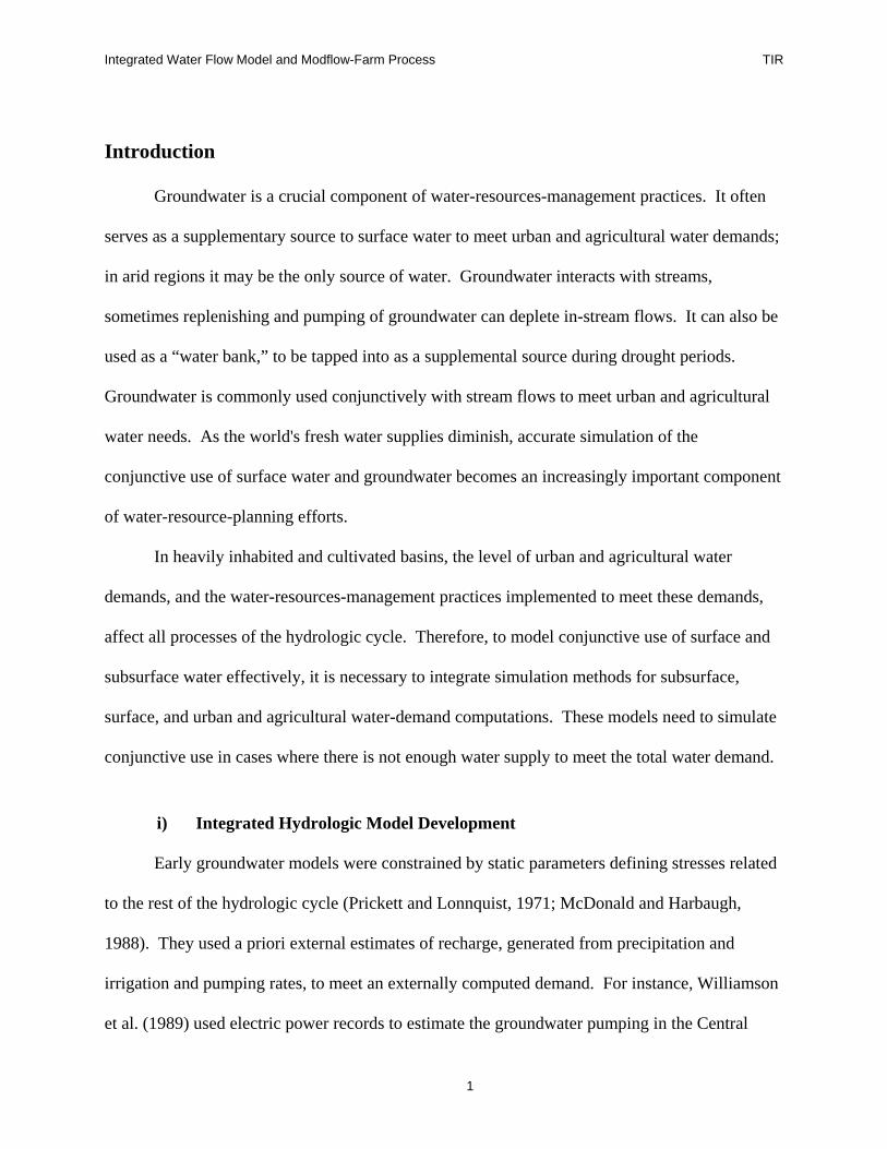
Introduction
Groundwater is a crucial component of water-resources-management practices. It often
serves as a supplementary source to surface water to meet urban and agricultural water demands;
in arid regions it may be the only source of water. Groundwater interacts with streams,
sometimes replenishing and pumping of groundwater can deplete in-stream flows. It can also be
used as a “water bank,” to be tapped into as a supplemental source during drought periods.
Groundwater is commonly used conjunctively with stream flows to meet urban and agricultural
water needs. As the world's fresh water supplies diminish, accurate simulation of the
conjunctive use of surface water and groundwater becomes an increasingly important component
of water-resource-planning efforts.
In heavily inhabited and cultivated basins, the level of urban and agricultural water
demands, and the water-resources-management practices implemented to meet these demands,
affect all processes of the hydrologic cycle. Therefore, to model conjunctive use of surface and
subsurface water effectively, it is necessary to integrate simulation methods for subsurface,
surface, and urban and agricultural water-demand computations. These models need to simulate
conjunctive use in cases where there is not enough water supply to meet the total water demand.
i) Integrated Hydrologic Model Development
Early groundwater models were constrained by static parameters defining stresses related
to the rest of the hydrologic cycle (Prickett and Lonnquist, 1971; McDonald and Harbaugh,
1988). They used a priori external estimates of recharge, generated from precipitation and
irrigation and pumping rates, to meet an externally computed demand. For instance, Williamson
et al. (1989) used electric power records to estimate the groundwater pumping in the Central
Integrated Water Flow Model and Modflow-Farm Process TIR
2
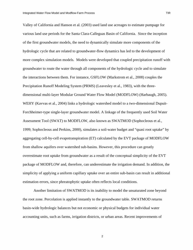
Valley of California and Hanson et al. (2003) used land use acreages to estimate pumpage for
various land use periods for the Santa Clara-Calleguas Basin of California. Since the inception
of the first groundwater models, the need to dynamically simulate more components of the
hydrologic cycle that are related to groundwater-flow dynamics has led to the development of
more complex simulation models. Models were developed that coupled precipitation runoff with
groundwater to route the water through all components of the hydrologic cycle and to simulate
the interactions between them. For instance, GSFLOW (Markstrom et al., 2008) couples the
Precipitation Runoff Modeling System (PRMS) (Leavesley et al., 1983), with the three-
dimensional multi-layer Modular Ground Water Flow Model (MODFLOW) (Harbaugh, 2005).
WEHY (Kavvas et al., 2004) links a hydrologic watershed model to a two-dimensional Dupuit-
Forchheimer-type single-layer groundwater model. A linkage of the frequently used Soil Water
Assessment Tool (SWAT) to MODFLOW, also known as SWATMOD (Sophocleous et al.,
1999; Sophocleous and Perkins, 2000), simulates a soil-water budget and “quasi root uptake” by
aggregating cell-by-cell evapotranspiration (ET) calculated by the EVT package of MODFLOW
from shallow aquifers over watershed sub-basins. However, this procedure can greatly
overestimate root uptake from groundwater as a result of the conceptual simplicity of the EVT
package of MODFLOW and, therefore, can underestimate the irrigation demand. In addition, the
simplicity of applying a uniform capillary uptake over an entire sub-basin can result in additional
estimation errors, since phreatophytic uptake often reflects local conditions.
Another limitation of SWATMOD is its inability to model the unsaturated zone beyond
the root zone. Percolation is applied instantly to the groundwater table. SWATMOD returns
basin-wide hydrologic balances but not economic or physical budgets for individual water
accounting units, such as farms, irrigation districts, or urban areas. Recent improvements of
Integrated Water Flow Model and Modflow-Farm Process TIR
3
exchanging the characteristics of SWAT hydrologic response units with MODFLOW cells (Kim
et al., 2008) have not changed most of the limitations described above. The outer boundaries of
models based on SWATMOD, which is now called SWAT-MODFLOW, are limited to
watershed boundaries. Some constraints on surface- and groundwater supply are present in
SWAT-MODFLOW, but a simulation of surface-water rights seniorities, or rate or head
constraints on pumpage from multi-aquifer wells, are not present. Another limitation is that the
recent improvements to the new SWAT-MODFLOW include head-dependent boundary flow.
However, this condition is simulated only with the stage-invariable RIVER package instead of
the stage-variable Streamflow Routing Package (SFR; Niswonger and Prudic, 2005). This limits
the ability to realistically simulate stream-flow responses to stresses due to changing hydrologic
conditions, such as diversions to meet the water demands and surface runoff into streams
generated by precipitation and irrigation.
Another model that links surface and groundwater components is MIKE SHE (Systeme
Hydrologique European), which is used to simulate flow and the transport of solutes and
sediments in both surface water and groundwater (DHI 1999). However, Said et al. (2005) points
out that MIKE SHE does not have the ability to handle variable grids and that its ability to
simulate evapotranspiration and stream-aquifer interaction could be improved (Prucha, 2004).
The stream-aquifer interaction is calculated using a conductance and the head difference between
the river—considered a line source—and the aquifer (Illangasekare, 2001). This approach is
similar to that used in the RIVER Package of MODFLOW, meaning stage is prescribed and not
dynamically dependent on stream-aquifer leakage and other inflows and outflows. MIKE SHE is
a physically based, fully distributed parameter model. It uses the 1-D Richards' equation for
unsaturated flow, which requires an extensive set of physical parameters. Often, some of the soil-
Integrated Water Flow Model and Modflow-Farm Process TIR
4
water constitutive parameters are not available, which makes it difficult to set up a fully coupled
MIKE SHE model. Among the coupled surface and groundwater models described above, MIKE
SHE is probably the most fully coupled hydrologic model; it includes an irrigation module, but
its downsides are its lack of a fully dynamic stream-aquifer interaction between variable stages
and variable heads, it does not return economic or physical mass balances for water-accounting
units, and it suffers from extensive data and parameter requirements.
HydroGeoSphere (Therrien et al., 2007) and ParFlow-CLM (Maxwell and Miller, 2005;
Kollet and Maxwell, 2008) are also among the integrated hydrologic models. These models solve
the three-dimensional Richard’s equation for the variably saturated subsurface flow
simultaneously with the conservation equations for land surface flow processes. Simultaneous
solution of surface and subsurface flow equations avoids the need to iterate between individual
flow models and provides a robust simulation mechanism. Since both HydroGeoSphere and
ParFlow-CLM solve Richard’s equation for the subsurface flow, the simulation time steps are
generally expressed in fractions of a second. For large basins with long simulation periods, such
a small magnitude for the time step may lead to very long computer run times. Even though both
models use fast matrix solvers, and ParFlow-CLM offers parallel processing features, the long
computer run times make these models primarily research tools.
The models described above all include the simulation of the land use based runoff
processes and the plant consumptive use, and their effects on groundwater dynamics. However,
they do not simulate agricultural and urban water demands on the basis of water-accounting units
and the conjunctive use of surface and subsurface water resources to meet these demands.
Essentially, they are descriptive models; i.e., given all the stresses on the hydrologic system
modeled, they describe where and how fast the water flows. Models like SIMETAW (Synder et
Integrated Water Flow Model and Modflow-Farm Process TIR
5
al., 2005) or methods described by Allen et al. (1998), on the other hand, simulate the
agricultural crop consumptive water requirements; however, they do this by separating the root
zone from the rest of the hydrologic cycle, neglecting the uptake from groundwater, and
assuming that the crop water requirement is met at every simulation time step without actual
knowledge of the potential sources of water supply.
To effectively model conjunctive use of surface and subsurface water resources to meet a
computed or pre-specified water demand, it is necessary to simulate two types of water balances
in the system: i) the physical mass balance in the system, which the descriptive models
mentioned above simulate, and ii) the economic balance between water demand and water
supply, which models like SIMETAW (Synder et al., 2005) simulate with the assumption that
supply is always available and is equal to demand. Additionally, for effective simulation of
conjunctive use, it is necessary to develop a model that is both descriptive and prescriptive. For
instance, in water resources planning studies, defining the sources of water (in terms of stream
diversions and pumping) to meet a predicted water demand, while honoring water rights and
environmental regulations, is as important as predicting the water demand itself.
ii) IWFM and MF-FMP Development
The California Department of Water Resources’ (CADWR) Integrated Water Flow
Model (IWFM) (Dogrul, 2009a, 2009b) and MODFLOW with the Farm Process (MF-FMP) of
the U.S. Geological Survey (USGS) (Schmid et al., 2006; Schmid and Hanson, 2009a, 2009b)
are two models that were developed to address the physical and economic water balance in a
watershed. These models allow the user to simulate physical flow processes of the hydrologic
system as well as simulate the water-resources-management practices in watersheds.
Integrated Water Flow Model and Modflow-Farm Process TIR
6
The roots of IWFM date back to a Ph.D. dissertation by Yoon (1976). IWFM’s precursor
was called the Integrated Groundwater Surface water Model (IGSM); after several modifications,
it was documented by Montgomery & Watson (MW, 1993). In 1990, the latest version of Yoon’s
original model was released as part of the Programmatic Environmental Impact Statement for the
Central Valley Project Improvement Act (CVPIA PEIS) funded by the U.S. Bureau of
Reclamation, CADWR, California State Water Resources Control Board (SWRCB), and the
Contra Costa Water District (CCWD). In 2001, after a thorough evaluation of IGSM, CADWR
developed and released its own version of the model that incorporated major changes to both the
theory and code of IGSM, called IGSM2, and later renamed IWFM (to distinguish it from other
versions of IGSM still in use). IWFM is a comprehensive model that effectively balances the use
of scientifically sound simulation methods with the ability to easily use readily available data in
model development, and has a flexible input file structure that incorporates time tracking and
other techniques to facilitate rapid revision of existing models for conducting feasibility and
impact assessments. It has been used to model the conjunctive-use programs and scenario
analysis in California’s Central Valley (Brush et al., 2008; Miller et al., 2009), and other
groundwater basins in California (BCDWRC, 2008a, 2008b) and Oregon (Jimenez, 2008).
MF-FMP uses MODFLOW-2000 (Harbaugh et al., 2000) and MODFLOW-2005
(Harbaugh, 2005). MODFLOW is a widely accepted, open-source, hydrologic model that has
been in use since 1988. Over a period of decades, many people from academia, government
agencies, and the private sector from all over the world have continuously contributed to its
development and bug fixes. It is the most used and trusted groundwater model in the world and
recently has been expanded to include more realistic coupling between surface and subsurface
processes. MF-FMP has been applied to four productive agricultural regions of different scale in
Integrated Water Flow Model and Modflow-Farm Process TIR
7
the states of California (Faunt et al., 2008, 2009a, 2009b, 2009c; Hanson et al., 2008) and New
Mexico (Schmid, 2004) to assess the availability of water and the impacts of alternative
management decisions.
Recently, both IWFM and MF-FMP have been used to model the water resources system
of the California Central Valley (Brush et al., 2008; Faunt et al., 2008, 2009a, 2009b, 2009c).
Both of these models were designed to assess the supply and demand components of the water-
resources system in the Central Valley, which include water use and movement on the land
surface, conjunctive use of surface and groundwater, and changes in groundwater storage and
land subsidence due to groundwater pumping. The two applications cover virtually the same
area, and the CADWR and USGS worked together during development of the two applications
to incorporate the same historic precipitation, surface-water inflow, and surface-water diversion
data to the extent that it was possible. Yet, even with similar input data, the two applications
yield some results that are similar and some that are different, owing in part to differences in the
conceptual framework of the two models, especially regarding the economic budgeting to match
water supplies and demands. At the level of complexity of the two applications, it was difficult to
track the sources of these differences. As part of an ongoing collaborative effort, the CADWR
and USGS started a comparison of the models discussed in this paper and a comparison of the
applications of the two models on a simple hypothetical problem (Schmid et al., 2011). This
paper compares the relevant conceptualizations and features of each hydrologic model pertaining
to groundwater, surface water and landscape processes, and the integrated simulation of water
demand and supply, water use, and movement. The implementation of these features for a
simple problem and comparison of results from the two models can be found in Schmid et al.
(2011).

Integrated Water Flow Model and Modflow-Farm Process TIR
8
Governing Equations
Conservation equations for groundwater, stream, lake, root zone, and land-surface runoff
processes are solved simultaneously in both models to simulate a large portion of the hydrologic
cycle, and the agronomic and human effects on the cycle. Among the mass conservation
equations, the groundwater-flow equation is the governing equation that is solved for
groundwater heads. Both models solve the same conservation equation for groundwater; IWFM
uses the finite-element approach, and MF-FMP uses the finite-difference approach. Conservation
equations for the other surface water and landscape flow processes are also solved at each
iteration until convergence of a groundwater-flow equation solver is reached. The solver is
assumed to have converged when a user-specified closure criterion is met for the difference
between results of successive iterations using the maximum absolute value of the change in
groundwater hydraulic heads and, optionally in MF-FMP, also of residual groundwater flows at
all nodes. With the coupled stream-groundwater conservation equations to simulate the stream-
aquifer interactions, both models are powerful tools to efficiently address important issues, such
as effects of conjunctive use programs, changes in irrigation methods, and implementation of
urban and agricultural water conservation programs, etc. on the hydrologic system modeled.
Both IWFM and MF-FMP simulate the vertical interaction between surface- and
groundwater across a vegetated root zone or non-vegetated unsaturated zone and across
streambeds. Alternatively, MF-FMP can simulate the infiltration across unsaturated zones
beneath stream beds (Niswonger and Prudic, 2005) and beneath large areas with unsaturated
zones (Niswonger et al., 2006). In the horizontal direction, both models simulate stream
diversions to agricultural and urban lands, and the surface runoff (i.e., rainfall runoff and
irrigation return flow) into streams. The models also simulate the conjunctive use of surface
Integrated Water Flow Model and Modflow-Farm Process TIR
9
water and groundwater to satisfy the consumptive use requirement of vegetation in excess of the
effective precipitation as well as urban water demands.
Although both models simulate the interaction between surface water and groundwater
across a root zone, the two models incorporate different conceptualizations of the conservation of
mass for root zone processes. Even though MF-FMP can be considered a fully coupled surface
and groundwater interactive hydrologic model, historically it originates from the groundwater
model MODFLOW. While stress periods can be of any length, solution time steps of long-term
regional MF-FMP models are commonly on the order of weeks or longer, as is typical for
regional hydrologic models used to analyze conjunctive use over decades. At these time steps,
and for medium root-zone depths, MF-FMP assumes all inflows into the root zone to be equal to
all outflow, on the basis of numerous HYDRUS-2D (Simunek et al., 1999) simulations for
various crop and soil types, root zone and capillary-fringe depths, water-table configurations, and
levels of potential evapotranspiration (Schmid, 2004; Schmid et al., 2006). In MF-FMP, inflows
that meet the crop evapotranspirative requirements are precipitation, irrigation, and root uptake
from groundwater. Outflows are transpiration and evaporation, runoff, and deep percolation
beneath the root zone.
In IWFM, the inflows are precipitation and irrigation, and the outflows are
evapotranspiration, runoff, and deep percolation. MF-FMP simulates uptake from groundwater
but does not simulate changes in the soil water storage. On the other hand, IWFM does not
simulate groundwater uptake but simulates changes in soil water storage. Land use processes in
both models are directly linked to the aquifer system, not only through deep percolation into the
groundwater but also through pumping to satisfy the agricultural and urban demands that are not
satisfied by surface water.
Integrated Water Flow Model and Modflow-Farm Process TIR
10
MF-FMP and IWFM have the option to neglect flow processes in the unsaturated zone
beneath the root zone and to assume instant recharge from deep percolation. However, both
models also feature an optional simulation of an unsaturated zone between the root zone and the
saturated aquifer system. MF-FMP simulates delayed recharge through a deep vadose zone
beneath root zones through a linkage to the Unsaturated Zone Flow package (Niswonger et al.,
2006; Schmid and Hanson, 2009b). Through the same linkage, MF-FMP also simulates
groundwater discharge to the surface and rejected infiltration from fully saturated conditions
under conditions of shallow or above-surface groundwater levels. IWFM features its own
unsaturated zone flow module that connects the root zone to the saturated groundwater system.
This module simulates the attenuation of deep percolation before it recharges a deep water table
or the rejection of infiltration in cases where the infiltration rates computed in the root zone
module are too high. The interaction between the root zone and unsaturated zone modules is a
one-way interaction, and no iterations between the two modules are performed. Vertical outflow
from the root zone module becomes inflow into the unsaturated zone module. Any part of the
inflow that is in excess of the available unsaturated zone storage or its conveyance capacity is
converted into surface runoff.
Both models also simulate the interaction between streams and groundwater. For stream
flow routing and stream-aquifer interaction across the streambed, MF-FMP uses the Streamflow
Routing Package, SFR (SFR1, Prudic et al., 2004; SFR2, Niswonger and Prudic, 2005) and
IWFM uses a method similar to that described in the SFR1 package. MF-FMP can also simulate
delayed recharge from infiltration beneath streambeds through a deep vadose zone (Niswonger
and Prudic, 2005). Although both models use similar approaches in stream-flow routing, the
Integrated Water Flow Model and Modflow-Farm Process TIR
11
following conceptual and implementation differences may lead to differences in the results of
both models:
i. The MF-FMP SFR package uses several options to define the relationship between
the stream stage and the flow (e.g., Manning’s equation with a rectangular channel or
an irregular-shaped cross section, either a rating table or a power function relating
both depth and width to stream flow). IWFM uses a user-specified rating table
between flow and stage; Manning’s equation can also be discretized through a rating
table.
ii. Both models express the stream-aquifer interaction as
st s ssg sg
K w LQ hd
= ∆ (1)
where Qsg is the flow rate between a stream section and the aquifer (L3T-1), Kst is the
hydraulic conductivity of the stream bed material (LT-1), ws is the width of stream
section (L), Ls is the length of stream section (L), d is the thickness of stream bed
material (L), ∆hsg is the vertical head difference between stream and the aquifer (L).
In both the SFR package and IWFM, ∆hsg is defined as the difference between the
head in the stream and the aquifer head. However, the representation of stream-
groundwater interaction when stream and aquifer are hydraulically disconnected is
different in both models. To comply with Darcy’s law in simulating flow through the
streambed, the SFR package assumes that the streambed is saturated at all times with
zero pressure at the bottom of the streambed. The SFR package represents the stream-
aquifer interaction when they are hydraulically disconnected as
sg st s s st s sd s sQ K w L K w L 1
d d+ = = +
(2)
Integrated Water Flow Model and Modflow-Farm Process TIR
12
where s is the stream stage (L).
Equation (2) assumes that the stream bed is saturated at all times. However,
following a prolonged drought the stream bed will be dry and it will require some
time for re-wetting. If the stream stage compared to the thickness of the stream bed is
small, such that s/d in equation (2) is much less than 1, most or all of the stream flow
will likely be used in re-wetting the stream bed and no seepage will occur. However,
using equation (2), a non-zero seepage rate will be computed that can be as large as
the stream flow itself. In MF-FMP, the streambed is assumed to be saturated at all
times, which, because of the large time steps used in most groundwater models, is
tantamount to assuming that the time for rewetting is short enough to not significantly
affect the modeled stream-aquifer water budget terms. IWFM, on the other hand,
approximates (2) as
sg st s ssQ K w Ld
≅
(3)
Although (3) is not an accurate representation of the Darcy equation, it does
produce lower seepage rates when the stream stage is small. It should be noted that
the offset between (2) and (3) is small in relation to Qsg when s/d is sufficiently larger
than 1, and that Qsg is equal in both codes if the stream and aquifer are hydraulically
connected. However both approaches used by SFR and IWFM assume instantaneous
recharge from beneath the streambed to the underlying aquifer.
iii. In MF-FMP, the user has the option to simulate delayed recharge from infiltration
beneath streambeds through a deep vadose zone (Niswonger and Prudic, 2005). First,
using this option imposes a constraint for the Darcy-type stream seepage across the
streambed as described above, which cannot exceed the vertical hydraulic
Integrated Water Flow Model and Modflow-Farm Process TIR
13
conductivity of the underlying unsaturated zone. Second, the infiltration into the
unsaturated zone between the streambed and the water table is converted to the water
content of leading or trailing waves of wetting or drying fronts by assuming that the
vertical flux is driven by gravitational forces only. The propagation of the waves is
then simulated by a kinematic wave approximation of vertical seepage through the
unsaturated zone. However, the water content cannot exceed the saturated water
content when the infiltration rate exceeds the saturated vertical hydraulic
conductivity.
Both models offer additional features for the simulation of other hydrologic processes
(e.g., simulation of open waters such as lakes and reservoirs and their interaction with the aquifer
system and the stream network). However, a comparison of these features is out of the scope of
this paper, and the interested reader is referred to the documentation of each model (Dogrul,
2009a, 2009b; Schmid et al., 2006; Schmid and Hanson, 2009a, 2009b; Harbaugh et al., 2000;
Harbaugh, 2005).
As well as vertical interactions between surface water and groundwater, lateral exchange
of water between land use processes and the stream network is provided in both models. Land
use processes in both models are directly linked to the stream network through direct runoff from
precipitation and agricultural return flow, and stream diversions to meet the water demand for
irrigated agriculture and irrigated urban landscape.
Comparison of Methods for Land Use and Root Zone Processes
Both IWFM and MF-FMP simulate most of the same flow processes of the hydrologic
cycle. However, there are both similarities and differences in the way these processes and their
Integrated Water Flow Model and Modflow-Farm Process TIR
14
interactions are conceptualized and simulated. In this section, a comparison of features and
simulation methods adopted by both models is presented. For the purposes of this report, the
comparison between these two models is generally limited to the flow processes that operate in
the control volume defined by the land surface and the vadose zone that extends to the water
table (Figs. 1 and 2). Furthermore, because of the complexity of both models, only the most
important components will be explained and compared. The reader is encouraged to consult
each model’s documentation for more information (Dogrul, 2009a, 2009b; Schmid et al., 2006;
Schmid and Hanson, 2009a, 2009b).
Both IWFM and MF-FMP consider two types of water budgeting for the control volume
horizontally delineated by land surface areas, called “subregions” in IWFM and “farms” in MF-
FMP. For both models, these water-accounting units can include irrigated and non-irrigated
farms, native vegetation, and urban areas. Using the term “farm” in MF-FMP” has become
somewhat of an anachronism as MF-FMP has advanced to types of water-accounting units other
than just agricultural farms. The water-accounting units in IWFM include the land surface area
and the root zone and, hence, are true control volumes, in MF-FMP, they do not include changes
in soil-water storage and, hence, are control interfaces at the land surface. There are two types of
budgeting associated with these water-accounting units (Figs. 1 and 2):
i. mass balance between all physical inflow and outflow components to and from the
control volume;
ii. economic balance between the irrigation water demand and the water supply from
different surface or groundwater components to meet this demand.
In the real world, the physical water balance is always achieved (i.e. mass is not created
or lost), whereas the economic balance may not be maintained. For instance, farmers may apply
Integrated Water Flow Model and Modflow-Farm Process TIR
15
more water than the true crop irrigation requirements, an unforeseen drought may limit
irrigation, non-irrigated lands that depend solely on precipitation may not get enough water in
drought seasons and get too much water in wet seasons, or overall source of water may be a
limiting factor.
The discussions below are centered on these two types of water budgeting. A summary of
the following comparisons between IWFM and MF-FMP is also given in the synoptic Table 2 at
the end of this report.
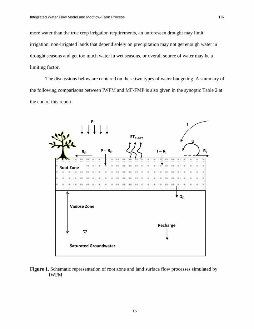
Figure 1. Schematic representation of root zone and land surface flow processes simulated by IWFM
Root Zone
Ri
U
P − RP RP I − Ri
I P
ETc-act
Recharge
Vadose Zone
Saturated Groundwater
DP
Integrated Water Flow Model and Modflow-Farm Process TIR
16
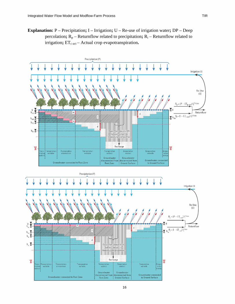
Explanation: P – Precipitation; I – Irrigation; U – Re-use of irrigation water; DP – Deep percolation; Rp – Returnflow related to precipitation; Ri – Returnflow related to irrigation; ETc-act – Actual crop evapotranspiration.
Integrated Water Flow Model and Modflow-Farm Process TIR
17
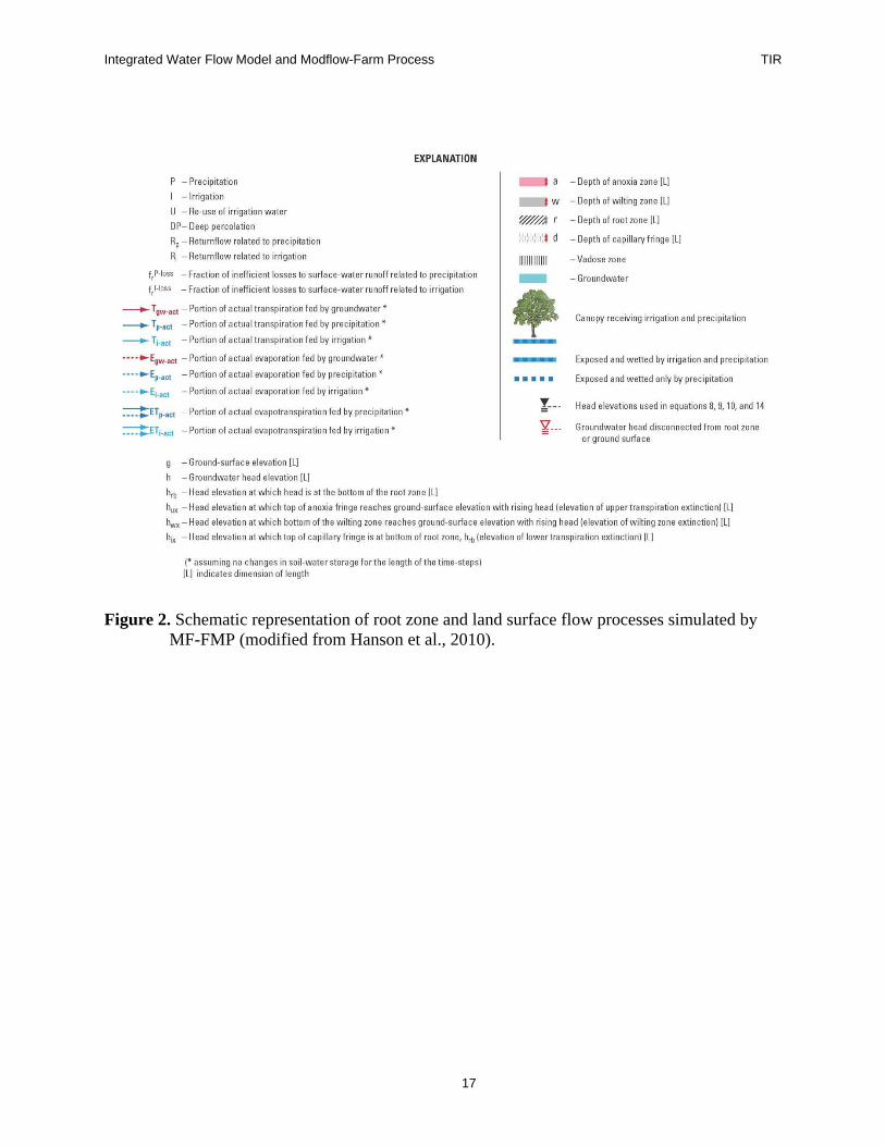
Figure 2. Schematic representation of root zone and land surface flow processes simulated by MF-FMP (modified from Hanson et al., 2010).
Integrated Water Flow Model and Modflow-Farm Process TIR
18
i) Framework and Distribution of Landscape Attributes
Both models adopt a land-use based approach to simulate the land surface and vadose
zone flow processes as well as water demands. The mesh cells (finite element cells in IWFM
and finite difference cells in MF-FMP) are grouped into “subregions” in IWFM and “farms” in
MF-FMP. Subregions and farms are the water budgeting units where irrigation water demands
are computed, and a balance between irrigation water supply and demand is sought; the supply-
demand balance may or may not be met depending on the amount of the supply with respect to
demand. In IWFM, subregions are also used as the smallest computation units for land surface
and root-zone flow processes where infiltration, precipitation runoff, agricultural return flow,
deep percolation, and evapotranspiration (ET) are calculated. In MF-FMP, farms are used as
budget units for all physical flows into and out of a farm. This includes natural flows and
irrigation-induced deliveries and return flows (Schmid and Hanson, 2009b). Inflows include
precipitation, non-, semi-, and fully-routed surface water deliveries, groundwater well pumping
deliveries, evaporation and transpiration from groundwater, and external deliveries from outside
the model domain (in case of a supply deficit). Outflows include evaporation and transpiration
components, respectively, fed by irrigation, precipitation, and uptake from groundwater, as well
as overland runoff and deep percolation.
Each mesh cell is assigned a soil type and related soil properties in each model. Soil
property values are user-specified in IWFM. These include four integer values representing the
basic characteristics of sands and gravels, fine and coarse textured soils, fine textured, and
impervious clays based on the classification system developed by the National Resources
Conservation Service (USDA, 1985), and basic soil-moisture properties such as a retention
parameter, field capacity, and total porosity similar to the HELP model (Schroeder et al., 1994).
Integrated Water Flow Model and Modflow-Farm Process TIR
19
MF-FMP uses words for soil types, for which the MF-FMP code contains intrinsic soil-type
specific coefficients. MF-FMP optionally allows the user to specify these coefficients. These
coefficients describe soil-type specific analytical solutions derived from HYDRUS-2D soil-
column models (Simunek et al., 1999; Schmid, 2004) that are used to calculate the reduction of
groundwater-influenced root uptake by conditions of anoxia or wilting at quasi-steady state
reached after time intervals of several days (Schmid et al., 2006; Schmid, 2004). These analytical
solutions also depend on the potential transpiration and on the depth of the total root zone. The
only other soil-type specific parameter in MF-FMP is the capillary fringe, which also contributes
to the depth of evaporation below the land surface.
In IWFM, each cell area is allocated among four pre-specified land use types:
agricultural, urban, native vegetation, and riparian vegetation. Agricultural lands are further
divided into user-specified crop types whose acreages are defined as time series data at the
subregional level. Physical and agricultural management properties for each crop are time-series
data specified by the user (table 1; Dogrul, 2009a, 2009b; Schmid et al., 2006; Schmid and
Hanson, 2009a, 2009b). Using the subregional crop acreages, IWFM computes area-weighted
averages for physical and management properties, resulting in a representative agricultural crop
for each subregion. Land surface and root zone flow processes are calculated for each of the four
land use types in each subregion in an aggregate form. For the purpose of groundwater flow
simulation, however, the root zone flow computed at the subregional level is distributed to the
cell level using the land use specified for each cell. Optionally, each element can be designated
as a separate subregion, making the areal resolution of the root zone in IWFM equivalent to that
of the underlying groundwater module, and closer in resolution to individual cell values specified
by that of MF-FMP.

Integrated Water Flow Model and Modflow-Farm Process TIR
20
In MF-FMP, each cell is assigned a user-defined crop-type ID, which may be constant or
change by stress period to simulate temporal and areal changes in cropping patterns within the
farm. The crop can be irrigated or non-irrigated. Irrigated crop types can also be “virtual crops”
used, for instance, to simulate water deliveries to zero-transpiration “crops” that represent
artificial recharge systems (Hanson et al., 2008, 2010). Non-irrigated crops can represent rain-fed
agriculture (i.e. dry-land farming) or native vegetation. Physical properties for all crops and
management practices (table 1) for agricultural crops are all user-defined on a cell-by-cell basis;
thus, MF-FMP computes landscape processes at the cell level
Table 1. -- Summary of crop physical and management properties for IWFM and
MF-FMP models (==== not included as a model input attribute).
Crop Properties (IWFM)
Crop Properties (MF-FMP)
Management Properties (IWFM)
Management Properties (MF-FMP)
Root-zone depth Root-zone depth Crop application Efficiency
Irrigation Efficiencies
==== Fraction of Transpiration ==== Fractions of inefficient losses as runoff from Precipitation
==== Fraction of Evaporation from Precipitation
==== Fractions of inefficient losses as runoff from Irrigation
==== Fraction of Evaporation from Irrigation
Fractions of inefficient losses as runoff from Irrigation re-used
====
Fraction of Field Capacity as Minimum Soil Moisture Requirement (i.e. wilting only) Volume-based properties
Stress-Response Function Values for Saturated and Unsaturated Root Zones (Zero uptake at Anoxia, Minimum pressure for full uptake, Maximum pressure for full uptake, and Wilting) Pressure-based properties
Potential Crop Evapotranspiration
Potential Crop Evapotranspiration
Consumptive Use
==== Crop Coefficients Acreage of irrigated crops Irrigated or non-irrigated
crop flag
Integrated Water Flow Model and Modflow-Farm Process TIR
21
ii) Computation of Land Surface and Root-Zone Components
For a given computational unit (a particular land use area in a given subregion for
IWFM, and a cell for MF-FMP), the general mass-balance equation that both models are based
on for the root zone is the following:
t 1 tt 1 t 1 t 1 t 1 t 1 t 1
gw act c actP I ET ET R DPt
++ + + + + +
− −
θ − θ+ + − − − =
∆ (4)
and
t 1 t 1 t 1p iR R R+ + += + (5)
where P is precipitation (LT-1), I is irrigation water (LT-1), ETgw-act is root uptake from
groundwater (LT-1), ETc-act is the total actual crop evapotranspiration (LT-1), R is the runoff from
precipitation and irrigation (LT-1), Rp is the surface runoff from precipitation (LT-1), Ri is the
irrigation surface return flow (LT-1), DP is the deep percolation that leaves the root zone as the
moisture moves downward (LT-1), t 1+θ is the soil moisture at the end of a time step (L), tθ is the
soil moisture at the beginning of a time step (L), ∆t is the time step length (T), and t is the time
step index (dimensionless).
In IWFM, equation (4) is solved for each subregion iteratively for each time step. IWFM
does not consider uptake from groundwater and ETgw-act in equation (4) drops out:
t 1 tt 1 t 1 t 1 t 1 t 1
c actP I ET R DPt
++ + + + +
−
θ − θ+ − − − =
∆ (6)
In MF-FMP, equation (4) is solved for each cell at each iteration (equation 7) because
many of the terms depend directly or indirectly on the elevation of the groundwater head, h.
ETgw-act and ETc-act vary with groundwater head where the water table is shallow enough to
evaporate and(or) be transpired. Since applied irrigation (I) and returnflows from excess
irrigation (R and DP) depend on ET(h) terms as part of the irrigation requirement calculation,
Integrated Water Flow Model and Modflow-Farm Process TIR
22
these terms depend indirectly on groundwater head. The following sections (c through f) explain
the dependencies of the actual ET components (ETc-act(h) and ETgw-act(h) ) on the head from the
irrigation delivery requirement (I(h)) and explain the dependencies of the crop irrigation
requirement ( ETi-act(h)) on the actual ET, runoff returnflow (R(h)), deep percolation (DP(h)),
and irrigation delivery requirement (I(h)) for MF-FMP.
MF-FMP does not consider changes in soil-water storage in the root zone (i.e., RHS in
equation (7) = 0):
( )k 1 k 1 k k 1 k k 1 k k 1 k k 1 kgw act c actP I h ET (h ) ET (h ) R (h ) DP (h ) 0+ + + + + +
− −+ + − − − = (7)
MF-FMP does simulate changes in storage in the deeper vadose zone below the root zone
through a linkage to the Unsaturated Zone Flow package (Niswonger et al., 2006) by treating
deep percolation out of the root zone as quasi-infiltration into the deeper vadose zone.
A comparison of how each term in equation (4) is computed in IWFM and MF-FMP is
given in the following sections. Some flow terms depend on others; therefore, the description of
these terms below is arranged accordingly. For simplicity, indices for time step (t) and iteration
(k) are dropped in the expressions that follow. Variable names have been simplified for use in
this document relative to those in the user guides (Dogrul 2009a, 2009b; Schmid et al., 2006;
Schmid and Hanson 2009b).
a) Precipitation, P
In both models, precipitation is a user-specified time series for each cell. In IWFM,
precipitation values are aggregated over four land use areas (agricultural, urban, native
vegetation, and riparian vegetation) in each subregion. In MF-FMP there is only one land-use per
model cell and the precipitation is used directly with that land use and associated attributes.
Integrated Water Flow Model and Modflow-Farm Process TIR
23
b) Rate of change of soil moisture, + −
t 1 t
tθ θ
∆
IWFM
IWFM simulates the rate of change in soil moisture by implicitly solving equation (6) for
t 1+θ . Equation (6) is a non-linear conservation equation because both ETc-act and deep
percolation, DP (as discussed below), are functions of t 1+θ . IWFM uses the Newton-Raphson
method to linearize and iteratively solve equation (6) for t 1+θ . It should be noted that the
iterative solution of equation (6) in IWFM is separate from the iterative solution of the linked
groundwater and stream-flow equations. Since none of the terms in equation (6) are dependent
on the groundwater head, there is no need to iterate between the root-zone and groundwater
modules. Instead, for each iteration of the simultaneous solution of the groundwater and stream-
flow equations, equation (6) is solved once (iteratively, since it is a non-linear equation) for the
soil moisture and flow processes in the root zone. As the solution for the groundwater and stream
flow equations converge so do the pumping and diversion rates that are used to compute I in (6),
and other root zone flow terms that depend on I.
MF-FMP
Unlike IWFM, MF-FMP does not simulate the rate of change in soil moisture in the root
zone. MF-FMP is currently limited to time steps of several days or longer, commonly used in
groundwater modeling, and was not designed to simulate root-zone processes in deep root zones
(on the order of several meters) with high soil-water storage potential that require simulation on
the order of minutes to days. MF-FMP assumes quasi-steady state conditions in the root zone on
the basis of findings from transient HYDRUS-2D soil-column models representing shallow- to
medium-depth root zones (Schmid et al., 2006). Simulated inflows into the root zone converged
Integrated Water Flow Model and Modflow-Farm Process TIR
24
to outflows after time intervals of several days, the minimum time step commonly used in
groundwater modeling. Hence, for these conditions in MF-FMP, the rate of change in soil
moisture is not tracked.
c) Evapotranspiration, ETc-act and ETgw-act
Crop evapotranspiration (ET) is conceptualized differently in the two models. IWFM
treats evaporation and transpiration as a combined flux; whereas, MF-FMP decomposes ET into
three separate evaporation (E) and three transpiration (T) flux components from precipitation,
irrigation, and groundwater uptake.
IWFM
IWFM treats ET as a single outflow component. ETc-pot is specified by the user as a time
series data set for each crop in each subregion. Although these estimates can be taken as the
crop ET under standard conditions, ETc, described by Allen et al. (1998), they can also be taken
as the crop ET under non-standard conditions, ETc-adj, also described by Allen et al. (1998), to
incorporate local conditions such as non-uniform irrigation, low soil fertility, salt toxicity, pests,
diseases, etc. (except in cases where the plants are water-stressed because of lack of sufficient
water; this situation is simulated dynamically in IWFM as discussed below). In essence, ETc-pot
values specified as input data to IWFM represent crop evapotranspirative requirements for a
target yield under known local soil, plant, and management conditions. Using user-specified crop
ETc-pot values, an average ETc-pot, weighted with respect to crop areas, is computed for each
subregion. Averaging of ETc-pot values is performed only for agricultural crops. Values for
urban lands, native vegetation and riparian vegetation in each subregion remain unchanged.
IWFM computes an ETc-act as a function of the soil moisture in the root zone:
Integrated Water Flow Model and Modflow-Farm Process TIR
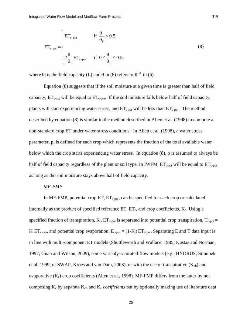
25
c potf
c act
c potf f
ET if 0.5
ET
2 ET if 0 0.5
−
−
−
θ> θ=
θ θ ≤ ≤θ θ
(8)
where θf is the field capacity (L) and θ in (8) refers to t 1+θ in (6).
Equation (8) suggests that if the soil moisture at a given time is greater than half of field
capacity, ETc-act will be equal to ETc-pot. If the soil moisture falls below half of field capacity,
plants will start experiencing water stress, and ETc-act will be less than ETc-pot. The method
described by equation (8) is similar to the method described in Allen et al. (1998) to compute a
non-standard crop ET under water-stress conditions. In Allen et al. (1998), a water stress
parameter, p, is defined for each crop which represents the fraction of the total available water
below which the crop starts experiencing water stress. In equation (8), p is assumed to always be
half of field capacity regardless of the plant or soil type. In IWFM, ETc-act will be equal to ETc-pot
as long as the soil moisture stays above half of field capacity.
MF-FMP
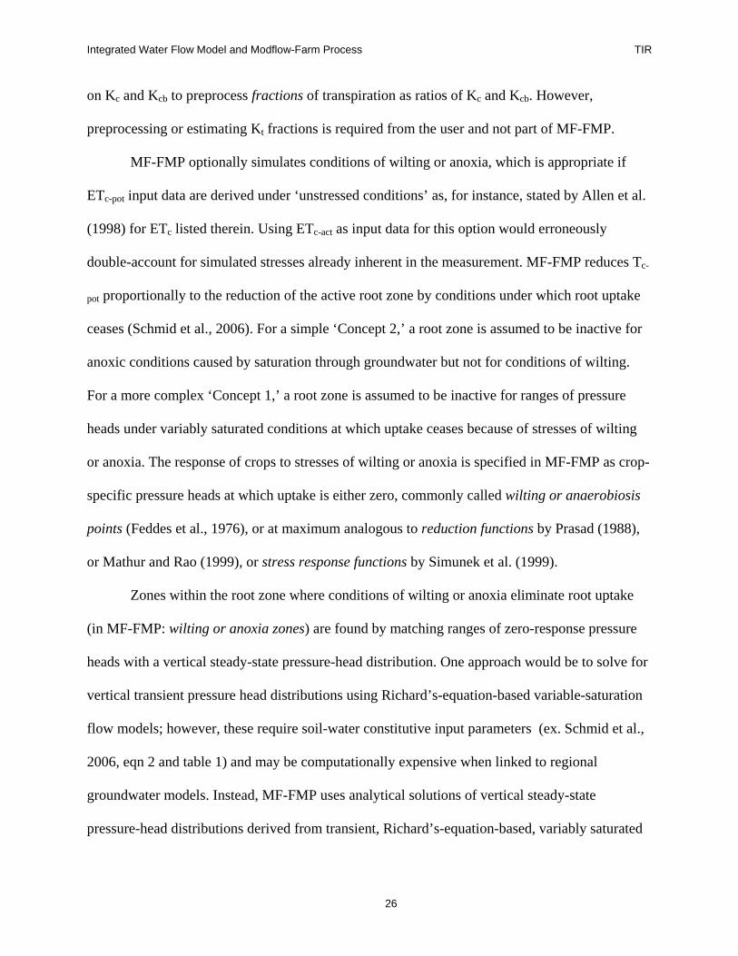
In MF-FMP, potential crop ET, ETc-pot, can be specified for each crop or calculated
internally as the product of specified reference ET, ETr, and crop coefficients, Kc. Using a
specified fraction of transpiration, Kt, ETc-pot is separated into potential crop transpiration, Tc-pot =
Kt ETc-pot, and potential crop evaporation, Ec-pot = (1-Kt) ETc-pot. Separating E and T data input is
in line with multi-component ET models (Shuttleworth and Wallace, 1985; Kustas and Norman,
1997; Guan and Wilson, 2009), some variably-saturated-flow models (e.g., HYDRUS, Simunek
et al, 1999; or SWAP, Kroes and van Dam, 2003), or with the use of transpirative (Kcb) and
evaporative (Ke) crop coefficients (Allen et al., 1998). MF-FMP differs from the latter by not
composing Kc by separate Kcb and Ke coefficients but by optionally making use of literature data
Integrated Water Flow Model and Modflow-Farm Process TIR
26
on Kc and Kcb to preprocess fractions of transpiration as ratios of Kc and Kcb. However,
preprocessing or estimating Kt fractions is required from the user and not part of MF-FMP.
MF-FMP optionally simulates conditions of wilting or anoxia, which is appropriate if
ETc-pot input data are derived under ‘unstressed conditions’ as, for instance, stated by Allen et al.
(1998) for ETc listed therein. Using ETc-act as input data for this option would erroneously
double-account for simulated stresses already inherent in the measurement. MF-FMP reduces Tc-
pot proportionally to the reduction of the active root zone by conditions under which root uptake
ceases (Schmid et al., 2006). For a simple ‘Concept 2,’ a root zone is assumed to be inactive for
anoxic conditions caused by saturation through groundwater but not for conditions of wilting.
For a more complex ‘Concept 1,’ a root zone is assumed to be inactive for ranges of pressure
heads under variably saturated conditions at which uptake ceases because of stresses of wilting
or anoxia. The response of crops to stresses of wilting or anoxia is specified in MF-FMP as crop-
specific pressure heads at which uptake is either zero, commonly called wilting or anaerobiosis
points (Feddes et al., 1976), or at maximum analogous to reduction functions by Prasad (1988),
or Mathur and Rao (1999), or stress response functions by Simunek et al. (1999).
Zones within the root zone where conditions of wilting or anoxia eliminate root uptake
(in MF-FMP: wilting or anoxia zones) are found by matching ranges of zero-response pressure
heads with a vertical steady-state pressure-head distribution. One approach would be to solve for
vertical transient pressure head distributions using Richard’s-equation-based variable-saturation
flow models; however, these require soil-water constitutive input parameters (ex. Schmid et al.,
2006, eqn 2 and table 1) and may be computationally expensive when linked to regional
groundwater models. Instead, MF-FMP uses analytical solutions of vertical steady-state
pressure-head distributions derived from transient, Richard’s-equation-based, variably saturated
Integrated Water Flow Model and Modflow-Farm Process TIR
27
soil-column models upon convergence of atmospheric and moving water-level boundary fluxes
after time intervals of several days. Soil-column models were developed using HYDRUS-2D
(Simunek et al., 1999) for various soil-specific soil-water constitutive parameters, crop-specific
stress-response functions, root-zone depths, depths to groundwater, and rates of potential
transpiration with groundwater as the only source for root uptake (Schmid, 2004). For
groundwater rising above the root-zone bottom, a wilting zone in the upper part of the root zone
decreased linearly, and an anoxia fringe above the water table remained constant until its top
reached ground surface. For other HYDRUS-2D simulations, infiltration (e.g., from precipitation
or irrigation) was added as an additional source for root uptake. However, the actual
transpiration, Tc-act, did not reach Tc-pot because infiltration wetting-fronts also can contain
pressure heads at which the crop’s response to anoxia reduces transpiration (Drew, 1997). Hence,
even for root zones not influenced by groundwater, Tc-act cannot exceed an anoxia-constrained
maximum possible Tc-act-max. Adding infiltration in excess of Tc-act-max resulted in transpiration-
inefficient losses. Tc-act-max might further be diminished if pressure heads of a wetting front are
higher than those of an anoxia fringe above a water table or where drainage takes place in lower
parts of the root zone that causes wilting.
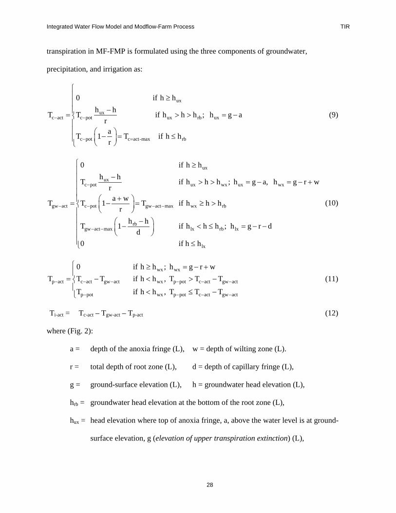
MF-FMP calculates a maximum actual transpiration (Tc-act; eq. (9)) and portions of
transpiration fed by uptake from groundwater (Tgw-act; eq. (10)), precipitation (Tp-act; eq. (11)),
and supplemental irrigation (Ti-act; eq. (12)), assuming no changes in soil-water storage over time
steps, and equal spatial distribution of roots and potential transpiration over the root zone. The
full development of these features is described by Schmid et al. (2006, figs 5-9) and Schmid and
Hanson (2009b, eqns 7-9, figs. 4 and 5). In summary, the estimate of actual from potential
Integrated Water Flow Model and Modflow-Farm Process TIR
28
transpiration in MF-FMP is formulated using the three components of groundwater,
precipitation, and irrigation as:
ux
uxc act c pot ux rb ux
c pot c act-max rb
0 if h hh hT T if h h h ; h g a
raT 1 T if h hr
− −
− =
≥
−= > > = − − = ≤
(9)
ux
uxc pot ux wx ux wx
gw act c pot gw act max wx rb
rbgw act max lx rb lx
0 if h hh hT if h h h ; h g a, h g r w
ra wT T 1 T if h h h
rh hT 1 if h h h ; h g r d
d0
−
− − − −
− −
≥
−> > = − = − +
+ = − = ≥ >
− − < ≤ = − −
lx if h h
≤
(10)
wx wx
p act c act gw act wx p pot c act gw act
p pot wx p pot c act gw act
0 if h h ; h g r wT T T if h h , T T T
T if h h , T T T− − − − − −
− − − −
≥ = − +
= − < > − < ≤ −
(11)
Ti-act = Tc-act – Tgw-act – Tp-act (12)
where (Fig. 2):
a = depth of the anoxia fringe (L), w = depth of wilting zone (L).
r = total depth of root zone (L), d = depth of capillary fringe (L),
g = ground-surface elevation (L), h = groundwater head elevation (L),
hrb = groundwater head elevation at the bottom of the root zone (L),
hux = head elevation where top of anoxia fringe, a, above the water level is at ground-
surface elevation, g (elevation of upper transpiration extinction) (L),
Integrated Water Flow Model and Modflow-Farm Process TIR
29
hwx = head elevation at which bottom of the wilting zone, w, is at ground-surface
elevation, g (elevation of wilting zone extinction) (L),
hlx = head elevation at which top of capillary fringe, d, is at bottom of root zone, hrb
(elevation of lower transpiration extinction) (L).
For ‘Concept 1,’ Tc-act varies linearly in eq. (9) between the elevation of upper
transpiration extinction, hux, and the elevation of the root-zone bottom, hrb. For heads below the
root-zone bottom, Tc-act is constant and reduced by the ratio between the anoxia fringe, a, and the
total root zone, r. In eq. (10), Tgw-act varies linearly between the elevation of upper transpiration
extinction, hux, and the elevation of wilting zone extinction, hwx. For heads between hwx and root-
zone bottom, Tgw-act is constant and reduced from Tc-pot to a maximum actual transpiration from
groundwater, Tgw-act-max, by the ratio between the sum of anoxia and wilting zones, a + w, and the
total root zone, r. Tgw-act also varies linearly between the head elevations between the root-zone
bottom and lower transpiration extinction, hlx. In eq. (11), Tp-act is equal to Tp-pot, except when
limited to the remainder of Tc-act that is not yet satisfied by transpiration fed by Tgw-act.
For ‘Concept 2,’ wilting and anoxia above the water level are not simulated (a = 0, w = 0
in eq. (9) and (10)), but Tc-pot is still linearly reduced to Tc-act (eq. (9)) or Tgw-act (eq. (10)) as the
active root zone is reduced by a rising water level. Tc-act equals Tc-pot for water levels below the
root-zone bottom, and Tgw-act reaches Tc-pot for water levels located at the root-zone bottom.
The actual evaporation from precipitation, Ep-act, is equal to the potential evaporation
from precipitation, Ep-pot, where precipitation in open areas exceeds Ep-pot, and equal to
precipitation in open areas where Ep-pot exceeds this precipitation. The potential evaporation from
irrigation, Ei-pot, can be reduced in open and exposed areas if not fully wetted. Evaporation
fractions of ETc-pot related to irrigation, Kei, can therefore be smaller than (1-Kt). If ET input data
Integrated Water Flow Model and Modflow-Farm Process TIR
30
reflect local wetting patterns of irrigation methods, and a reduction in evaporation is implicitly
accounted for, then the user should keep Kei = (1-Kt). In eq. (13), the actual evaporation from
irrigation, Ei-act, accounts for evaporative losses of irrigation and varies proportionally to the
transpirative irrigation requirement by a ratio of Kei and Kt:
Ei-act = Ti-act (Kei/Kt) (13)
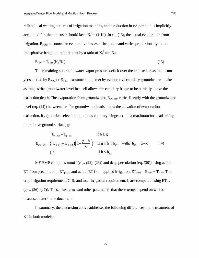
The remaining saturation water-vapor pressure deficit over the exposed areas that is not
yet satisfied by Ep-act or Ei-act is assumed to be met by evaporative capillary groundwater uptake
as long as the groundwater level in a cell allows the capillary fringe to be partially above the
extinction depth. The evaporation from groundwater, Egw-act, varies linearly with the groundwater
level (eq. (14)) between zero for groundwater heads below the elevation of evaporation
extinction, hex (= surface elevation, g, minus capillary fringe, c) and a maximum for heads rising
to or above ground surface, g:
( )c pot p act
gw act c pot p act ex ex
ex
E E if h g
g hE E E 1 if g h h , with: h g cc
0 if h h
− −
− − −
− ≥
+ = − − < < = −
≤
(14)
MF-FMP computes runoff (eqs. (22), (23)) and deep percolation (eq. (30)) using actual
ET from precipitation, ETp-act, and actual ET from applied irrigation, ETi-act = Ei-act + Ti-act. The
crop irrigation requirement, CIR, and total irrigation requirement, I, are computed using ETi-act
(eqs. (26), (27)). These flux terms and other parameters that these terms depend on will be
discussed later in the document.
In summary, the discussion above addresses the following differences in the treatment of
ET in both models:
Integrated Water Flow Model and Modflow-Farm Process TIR
31
i) IWFM calculates ET as a single term for a representative crop, computed by
area-weighted averaging of ET for individual crops within a subregion. MF-
FMP calculates six separate ET components of evaporation and transpiration
from precipitation, irrigation, and groundwater on a cell-by-cell basis within the
water accounting unit (i.e. a farm). The differences between the two models,
due to differing approaches in this context, can be minimized if each mesh cell
in IWFM is designated as an individual subregion.
ii) IWFM does not simulate ET from groundwater; whereas, MF-FMP does.
iii) IWFM does not simulate anoxic conditions but simulates wilting conditions by
reducing ETc-pot to ETc-act when soil moisture falls below half of field capacity.
MF-FMP always reduces ETc-pot to ETc-act to simulate the effects of conditions
of anoxia and wilting
iv) IWFM uses the user-specified ETc-pot values as the target crop consumptive use
to be met when calculating the irrigation water demand, while MF-FMP uses
computed ETc-act, for the same purpose.
d) Runoff, R
Overland runoff can be composed of several flow components, such as (a) direct runoff,
(b) interflow from excess precipitation and irrigation, (c) runoff generated by infiltration in
excess of the saturated hydraulic conductivity of the deeper unsaturated zone beneath the root
zone, and (d) runoff from groundwater discharge and from rejected infiltration in areas of high
groundwater levels. Neither IWFM nor MF-FMP capture all of these components. IWFM can
simulate runoff components (a) and (c) through its own root zone and unsaturated zone modules.
Historically, MF-FMP was developed to address flood and basin-level irrigation along the Rio
Integrated Water Flow Model and Modflow-Farm Process TIR
32
Grande of New Mexico, where slopes are small and direct runoff is negligible, but interflow
runoff can matter in different intensities for irrigation and precipitation (Schmid et al. 2009c).
Hence, MF-FMP simulates runoff component (b). Runoff components (c) and (d) are available in
MF-FMP through a linkage to the Unsaturated Zone Flow Package (Schmid and Hanson, 2009b)
but are not discussed further here as this linkage is optional for deeper vadose zones that extend
below the root zone.
IWFM
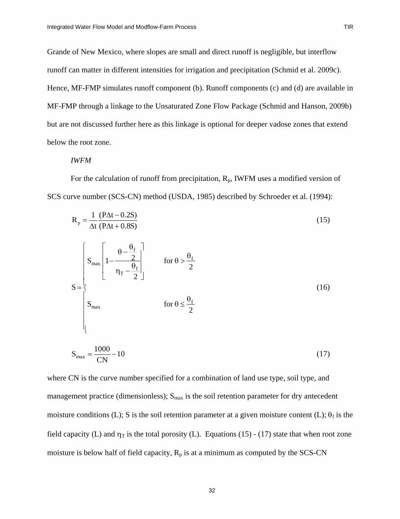
For the calculation of runoff from precipitation, Rp, IWFM uses a modified version of
SCS curve number (SCS-CN) method (USDA, 1985) described by Schroeder et al. (1994):
p1 (P t 0.2S)Rt (P t 0.8S)
∆ −=∆ ∆ +
(15)
f
fmax
fT
fmax
2S 1 for 2
2S
S for 2
θ θ− θ− θ > θ η −
= θ θ ≤
(16)
max1000S 10CN
= − (17)
where CN is the curve number specified for a combination of land use type, soil type, and
management practice (dimensionless); Smax is the soil retention parameter for dry antecedent
moisture conditions (L); S is the soil retention parameter at a given moisture content (L); θf is the
field capacity (L) and ηT is the total porosity (L). Equations (15) - (17) state that when root zone
moisture is below half of field capacity, Rp is at a minimum as computed by the SCS-CN
Integrated Water Flow Model and Modflow-Farm Process TIR
33
method. As the soil moisture increases above half of field capacity, the retention capacity of the
soil decreases and Rp increases.
In IWFM, the net return flow due to irrigation, Ri, is computed as
i i ini iR R U−= − (18)
where, Ri-ini is the initial return flow before a portion of it is captured and re-used, and Ui is the
re-used portion of the initial irrigation return flow. Ri-ini and Ui are computed based on user-
specified time series initial return flow and re-use factors, defined as a fraction of the prime
irrigation water (i.e., irrigation water before re-use occurs), I:
I inii ini rR I f −− = × (19)
Ii uU I f= × (20)
Substituting (19) and (20) into(18), Ri is expressed as
( )I ini I I ini Ii r u r uR I f f ; f f− −= − ≥ (21)
In (19) - (21), I inirf − and I
uf are the ratios of the initial return flow, i iniR − , and the re-used
return flow, iU , to the prime irrigation water, I, respectively. By explicitly modeling re-use with
equation (20), IWFM can represent irrigation water recycling practices in a regional simulation
where it would be impractical to model every single structure designed to capture the irrigation
return flows. Furthermore, such an approach is in line with the available data and design
practices for the return-flow-capturing structures (Schwankl et al., 2008). Both Rp and Ri are
used as inflows to stream reaches specified by the user, and they become available for
downstream diversions. This is equivalent to the method that can be used in MF-FMP to
represent re-use; it offers a second way to represent re-use in IWFM.
Integrated Water Flow Model and Modflow-Farm Process TIR
34
MF-FMP
MF-FMP computes R as the portion of crop-inefficient losses from precipitation or
irrigation that contribute to runoff:
P lossp p act rR (P ET )f −
−= − (22)
I lossi i act rR (I ET )f −
−= − (23)
where ETp-act and ETi-act are the portions of the ETc-act fed by precipitation or irrigation (LT-1),
respectively, and P lossrf − and I loss
rf − are fractions of the respective crop-inefficient losses from
precipitation or irrigation that go to runoff, given as time series data. Losses from precipitation
or irrigation that do not contribute to runoff are assumed to be deep percolation. MF-FMP
assumes that all precipitation or irrigation is initially available for crop evapotranspiration before
any runoff in the form of crop-inefficient losses occurs. Instead of specifying P lossrf − and I loss
rf −
manually, MF-FMP also provides an alternative option to calculate these fractions based on the
local (cell-by-cell) slope of the surface. In MF-FMP, irrigation return flow is routed to any user-
specified stream reach or, alternatively, to let MF-FMP search for a stream reach nearest to the
lowest elevation of the farm, where return flow is assumed to gather. The stream network is
simulated by a linkage between FMP and the Stream flow Routing Package of MODFLOW. Re-
use of irrigation return flow is not explicitly modeled in MF-FMP. However, the user has the
option to return the entire runoff from both precipitation and irrigation losses to points of
diversion either to the farm, from which the runoff originates, or to a downstream farm. This
way, runoff becomes available for diversions and can be re-used.
Irrigation return flow in MF-FMP is related to losses from irrigation, while in IWFM it is
related directly to the total irrigation. Assuming re-used return flow is zero and both MF-FMP
Integrated Water Flow Model and Modflow-Farm Process TIR
35
and IWFM yield the same irrigation return flow, the respective “runoff fractions” can be
translated into each other by equating (21) and (23):
I loss I inii act r r(I ET )f I f− −−− = × (24)
One important difference between the approaches of the two models is that IWFM
subtracts surface runoff from precipitation and irrigation before the computation of ETc-act, i.e.,
portions of precipitation and irrigation never contribute to crop evapotranspiration. MF-FMP, on
the other hand, assumes all precipitation and irrigation are initially available for crop
evapotranspiration and inefficient losses; runoff generated as portion of these inefficient losses is
computed after ETc-act is calculated.
e) Irrigation water, I
Irrigation water in both models can be specified as time series input data (in terms of
pumping, stream diversions, and water imported from outside the model domain), or
dynamically computed to satisfy the unmet agricultural crop consumptive requirement. MF-
FMP can also dynamically compute the irrigation water requirement for irrigated urban
landscape, whereas, in IWFM, urban water demand (both for outdoors and indoors usage) is
always user-specified as time series data. In MF-FMP, the unmet agricultural and irrigated urban
water demand is the portion of that demand after the contributions of precipitation and uptake
from groundwater to ETc-act are taken into account. In IWFM, it is the portion of the demand
after contributions of precipitation and soil moisture stored in the root zone to meet this demand
are taken into account. Both models distinguish between urban lands, agricultural crops, and
native vegetation so that I is specified or computed only for irrigated agricultural or urban lands.
In both models, if I is specified by the user, it will either be equal to, less than, or more
than the computed water demand. If the user chooses to let IWFM or MF-FMP compute I
Integrated Water Flow Model and Modflow-Farm Process TIR
36
internally, then it will be equal to the unmet agricultural water demand (and urban water demand
in the case of MF-FMP), given that there is no shortage of water (in terms of stream diversions,
groundwater pumpage, and imported water) in the modeled system. In this section, the methods
used by both models to compute the unmet water demand, and how I is related to it, will be
discussed. The situations where I is different from the unmet water demand will be discussed
later in this document.
IWFM
In IWFM, for agricultural lands, the user can choose to compute water demand
dynamically or specify it as a time series. The latter option is used in planning studies where the
demand is dictated by water rights and entitlements, rather than the actual crop
evapotranspirative requirements. The physical routing of irrigation water through the root zone
is still based on physical properties, such as ETc-pot, soil moisture, etc. In this approach, it is
possible that the water supply, to meet the water demand dictated by legal rights, will be
different than the actual crop evapotranspirative demand. It should be noted that specifying water
demands based on water rights or entitlements in IWFM does not imply that IWFM considers
water rights hierarchy and preferential water delivery. By using this option, the user simply
overrides water demands computed based on physical conditions (explained later in this
document) by water delivery amounts defined by legal rights. Each diversion/delivery has equal
priority in IWFM.
If the former option of dynamic water demand computation is chosen, IWFM uses an
irrigation scheduling-type approach. For each crop in a subregion, time series data of maximum
allowable depletion (MAD), defined as a fraction of the field capacity at which irrigation is
triggered (Allen et al., 1998), as well as time series irrigation period flag (equals 0 or 1) that
Integrated Water Flow Model and Modflow-Farm Process TIR
37
defines if it is irrigation season or not, are specified by the user. Similar to other crop properties,
MAD is averaged using a crop-area-weighted approach to come up with a representative MAD
for the subregion. In IWFM, crop-water demand is closely linked to the mass balance expressed
in equation (6). At the beginning of each time step, equation (6) is solved for t 1+θ with I and the
irrigation return flow, Ri, set to zero. If t 1+θ is computed to be greater than or equal to fMAD×θ
, then irrigation water demand is zero. Otherwise, an irrigation amount that is required to raise
the soil moisture up to θf is computed by setting t 1+θ to θf, using user-specified ETc-pot for ETc-act,
rearranging equation (4) with ETgw-act set to zero, and utilizing equations (5) and (21):
( )( )
tt 1 t 1 t 1 t 1f
p c pott 1
I ini Ir u
P R ET DPtI
1 f f
+ + + +−
+−
θ − θ− − − −
∆=− −
(25)
Equation (25) is used to compute irrigation water demand only for agricultural lands and
only for time steps where irrigation period flag is set to 1. Urban water demand is always a user-
specified time series data in IWFM.
MF-FMP
In MF-FMP, the crop irrigation requirement, CIR, is equal to the actual
evapotranspiration from irrigation, ETi-act, and is computed for each model cell and iteration at
each transient time step, assuming a quasi-steady state between all flows into and out of the root
zone that is reached at the end of time intervals typical in MODFLOW, as follows:
CIR = ETi-act =Ti-act + Ei-act (26)
where Ti-act is the portion of the actual transpiration supplied by irrigation (LT-1), and Ei-act is the
actual evaporation loss from irrigation (LT-1) proportional to Ti-act. The simulation of Ti-act and
Ei-act is discussed in detail in the previous section and expressed in equations (12) and (13).
Integrated Water Flow Model and Modflow-Farm Process TIR
38
MF-FMP calculates a total irrigation delivery requirement, I, for each cell at each
iteration of a particular time step as the evapotranspirative crop irrigation requirement that
depends on the groundwater head at the previous iteration divided by the on-farm efficiency of a
particular time step:
t,k 1 t,kt ,k 1 i act
t
ET (h )Ie
++ −= (27)
where e is the on-farm efficiency defined as the fraction of the total irrigation water that is used
beneficially in the farm. The total irrigation water demand for each farm is computed as cell
delivery requirements accumulated over all cells within the domain of a farm. CIR is computed
only for cells that have land use defined as either urban irrigated landscape or an irrigated
agricultural crop, and is zero for cells with non-irrigated land use.
Comparing (25) to (27), it can be seen that, in MF-FMP, I is calculated for each cell on
an iterative level based on a dynamically updated groundwater head-dependent evaporative crop
irrigation requirement, ETi-act, while in IWFM, I is calculated for a subregion based on user-
specified input data and independent of groundwater elevations.
Based on the discussion of irrigation water, I, and irrigation return flow, Ri, a correlation
between initial return flow fraction, I inirf − , in IWFM, and crop inefficiency losses due to
irrigation, I lossrf − , in MF-FMP, can be obtained. After substituting equation (25) into (24) for ETi-
act and rearranging the resulting equation, one can obtain
( )I loss
I ini I ini I lossi act rr r r
(I ET )ff f 1 e fI
−− − −−−
= ⇒ = − (28)
Integrated Water Flow Model and Modflow-Farm Process TIR
39
Hence, the initial return flow fraction, I inirf − , in IWFM, is linearly related to the fraction of
the crop inefficiency losses due to irrigation, I lossrf − , and in MF-FMP, by a proportionality factor
of 1-e, with e being the on-farm efficiency for the entire farm or for a specific crop on that farm.
f) Deep percolation, DP
IWFM
IWFM computes DP with a one-dimensional physical routing approach to compute the
deep percolation using Campbell’s method (Campbell, 1974):
2 3
u sT
DP K K
+ λλ θ
= = η (29)
where Ku is the unsaturated hydraulic conductivity (LT-1), Ks is the saturated hydraulic
conductivity (LT-1), ηT is the total porosity (L), θ is soil moisture (L), and λ is the pore size
distribution index (dimensionless). In (29), it is assumed that the vertical hydraulic gradient is
unity and residual water content (i.e., specific retention) is negligible.
As defined in equation (29), deep percolation is a function of soil moisture; it is
computed dynamically in IWFM. As shown in equation (25), it has a direct effect on computed
water demand. As it depletes soil moisture, it increases the computed water demand. The
irrigation water not only needs to meet the crop evapotranspirative requirements and bring the
soil moisture to field capacity, but it needs to compensate for water lost from the root zone
through deep percolation as well. As an example, growing a specified crop for a target yield on a
sandy soil will require more water than growing the same crop on a clayey soil for the same
target yield as a result of higher deep percolation rates. Recharge to groundwater in IWFM can
be instantaneous or it can optionally be delayed with the use of IWFM’s unsaturated zone
component (Dogrul, 2009a).
Integrated Water Flow Model and Modflow-Farm Process TIR
40
MF-FMP
MF-FMP computes DP as the sum of deep percolation below the root zone from
precipitation and irrigation, which can be instantaneous or delayed with linkage to the
unsaturated zone infiltration package, UZF (Niswonger et al, 2006). It is the user-specified
portion of losses of precipitation and irrigation that are not consumptively used by plants and not
lost to surface water runoff:
( ) ( )P loss I lossp act r i act rDP (P ET ) 1 f (I ET ) 1 f− −− −= − − + − − (30)
iii) Water Demand and Supply
In today’s world where fresh water sources are limited, questions that constantly arise in
densely populated and cultivated watersheds are related to the magnitudes of future urban and
agricultural water demands, i.e., if the available sources of water in terms of precipitation, stream
diversions, and groundwater pumping are sufficient to meet these demands. The answers for
these questions become harder to track with the presence of complicated surface water rights and
environmental regulations in the watershed. Typically, the hydrologic runoff processes in a basin
are controlled by the water-resources-management practices used to meet the water demand
while honoring surface-water rights and environmental regulations on stream-flow quantities.
In the real world, computed or estimated water demands and available water supplies
don’t always balance. For instance, water agencies generally have surface-water rights defined
by laws that may or may not equal their actual water demand. In severe drought years, farmers
may not receive all the water they need for a target crop yield, creating a supply deficit.
Conversely in wet years, farmers may have more water delivered than is needed for irrigation to
sustain surface-water rights, sustain flushing of saline soils, or to enhance deep percolation for
Integrated Water Flow Model and Modflow-Farm Process TIR
41
later groundwater pumpage. Non-irrigated areas with natural vegetation rely solely on
precipitation, which may be more or less than the actual plant evapotranspirative requirement.
Both IWFM and MF-FMP are designed to address (i) most of the issues regarding the
computation of water demand, (ii) configuration of different sources of water supply to meet this
demand, and (iii) computation of the hydrologic effects of unbalanced demand and supply. The
next section discusses features in each model representing total water demand, water supply
components, and the balance between supply and demand components.
a) Total water demand
In addition to irrigation water demand, both IWFM and MF-FMP also allow non-
irrigation demand, such as urban, municipal, and industrial water demand, to contribute to the
total requested demand that needs to be met with surface water and groundwater supply
components.
IWFM
Urban-water demand is always represented by user-specified time series data in IWFM.
This approach is in line with available data and methods for the prediction of urban-water
demand. Although a similar approach as in equation (25) can be used for computing urban-water
demand for parks, residential yards, etc., urban-water demand is often described as a function of
population and expressed in terms of water use per capita per day (e.g., CADWR, 1998). By
requiring urban-water demand as input data, IWFM allows the user to utilize standard methods
for urban-water demand predictions. The fraction of the total urban-water demand that is used
for municipal and industrial needs is specified by the user as time series data. It should also be
noted that agricultural and urban demands in a subregion are not lumped in IWFM. Instead,
IWFM attempts to meet both demands separately.
Integrated Water Flow Model and Modflow-Farm Process TIR
42
MF-FMP
In MF-FMP, other non-crop urban-water demand can be factored into the data input for
so-called non-routed deliveries. That is, if non-routed external water transfers are known, then
the municipal and industrial water demand needs to be subtracted first. The result is then the
input in MF-FMP for non-routed deliveries. This may mean that more urban-water demand is
subtracted than water transfers available. A negative non-routed delivery indicates a shortage
that needs to be satisfied along with water demand for urban irrigated landscape by other second
and third-level delivery components, that is, routed surface water and pumped groundwater.
Another non-agricultural water demand can be the target percolation rate of a percolation
pond or of a set of injection wells of an Aquifer-Storage-and-Recovery System (ASR). This
demand can be simulated as a “design” irrigation demand of a “virtual zero-transpiration crop”
that is based on the known maximum infiltration rate of the ASR pond or injection wells
(Hanson et al., 2008). These and other non-routed deliveries are accounted for separately for
each farm.
b) Water-supply components
The initial sources of water to meet the total water demand come from precipitation in
both models, soil moisture stored in root zone in IWFM, and root uptake from groundwater in
MF-FMP. Any unmet demand in both models is satisfied by water imported from outside the
model area, stream diversions, and groundwater pumping; referred to as water-supply
components in this report.
IWFM
In IWFM water can be imported into the modeled system from outside sources that are
not simulated. Diversions and pumping that occur in the modeled area also can be used as water
Integrated Water Flow Model and Modflow-Farm Process TIR
43
supply to meet the demand. IWFM offers two types of pumping: well pumping and element
pumping. Well pumping can be used when pumping from individual wells is simulated. Each
well is defined with its coordinates, radius and screening depths. User-specified time series
pumping rates are also assigned to each well. In cases where the screened interval of a well
intersects with multiple aquifer layers, the Kozeny equation (Driscoll, 1986; Dogrul, 2009a) is
used to distribute the pumping rate to individual aquifer layers. Element pumping can be used in
regional modeling studies where simulation of individual wells is not practical, or the necessary
information for all wells is not available. Element pumping allows the user to specify time series
pumping rates at specific mesh elements based on the estimated agricultural water demand
within that element. In essence, this option represents pumping from a cluster of wells that are
located in a mesh element. Pumping defined at an element is distributed to the surrounding
nodes using the fractions of element area associated with each node. These fractions are
computed as part of the implementation of the finite element method. The distribution of
pumping rate to individual aquifer layers is specified by the user. In a single model study, both
well pumping and element pumping can be utilized.
IWFM associates each source of water supply with a target subregion and a time series
irrigation fraction that allocates a portion of the supply to meet the agricultural demand. The rest
of the supply is used to meet the urban demand in the subregion. Any water supply that is in
excess of irrigation water requirement will either increase the soil moisture, or become deep
percolation or irrigation return flow, based on the solution of the conservation equation (6).
IWFM allows both recoverable and non-recoverable losses specified for each water
supply as a user-defined fraction of the total supply amount. The recoverable losses represent
seepage from the conveyance system that ultimately becomes recharge to groundwater. The
Integrated Water Flow Model and Modflow-Farm Process TIR
44
non-recoverable losses represent evapotranspirative losses from the conveyance system. This
feature can also be used to simulate artificial recharge operations by designating a fraction or the
entire amount of the diversion or pumpage as recoverable loss and identifying the mesh elements
where these losses will be used as recharge to groundwater. The recoverable losses are
completely head-independent and recharge groundwater instantaneously. Alternatively, IWFM
allows part or all of a diversion to be diverted into a lake. Conservation equations for lakes are
solved simultaneously with groundwater and stream flow equations, and this feature can be used
for a head-dependent simulation of artificial recharge operations, such as spreading basins.
MF-FMP
MF-FMP simulates three types of water deliveries into farms that originate as stream
diversions: non-routed deliveries (NRD), semi-routed deliveries (SRD), or fully-routed deliveries
(RD). NRDs are deliveries that originate from any source outside the model domain; i.e., they
represent water imported into the modeled area. SRDs and RDs originate from streams within
the model domain. Multiple types of NRDs can be specified and are given farm identifiers (IDs)
they serve, maximum volumes, ranks in which sequence they are used, and information whether
to recharge potential excess from NRDs into the stream network or into injection wells.
Locations within the stream network from where SRDs are taken are specified by the user at
modeled stream reaches. RDs are automatically diverted to a farm from the uppermost stream
reach of either segments that are used for diversion only, or from any type of river segment that
is located within the domain of the respective farm. The last source of water, groundwater
pumping, comes from farm wells located at user-specified cells with specified maximum
pumping rates and farm IDs they serve.
Integrated Water Flow Model and Modflow-Farm Process TIR
45
MF-FMP first uses NRD types in sequence of their ranking to meet irrigation water
demand. This can indirectly include the pumpage, delivery, and reuse of stored groundwater
through ASR operations. Any unmet demand is then served by SRDs and finally by groundwater
pumping. The maximum rates specified for each source of water generally represent legal or
structural constraints on that source. NRDs are limited by the maximum rates specified for each
of them. SRDs (or alternatively RDs) are limited by the available stream flow or by legal
constraints such as equal appropriation allotment heights or prior appropriation calls. Diversion
rates specified for a diversion from a main stem river into a diversion segment are possible
through data input in the SFR Package. These “river-to-canal” diversions can be specified along
a segment near, or further upstream, from which the SDRs or RDs. as “canal-to-farm”
diversions, occur. Subject to any canal water losses or gains in between the “river-to-canal” and
“canal-to-farm” diversion, this mechanism can be used to construct a demand-driven and supply-
constrained surface-water delivery system that is implicitly linked to the potential amount of
water that is simulated to be conveyed in the stream to the point of diversion and delivery.
In MF-FMP, water is derived first from natural crop water-supply components such as
precipitation and uptake from groundwater and second from delivery requirement-driven supply
components (such as NRDs) and surface-water deliveries. All farm wells in MF-FMP are
associated with a farm through the Farm-ID and can thus be located inside or outside the farm.
The groundwater pumping of each farm equals the residual delivery requirement or the
cumulative maximum pumping capacity, whichever is less. The farm wells in MF-FMP can be
single-aquifer wells that pump from the center of the finite-difference cell or multi-node wells
which can represent non-uniform wellbore inflow from vertical multi-aquifer wells through a
linkage with the multi-node well package (MNW; Halford and Hanson 2002) that is both head-
Integrated Water Flow Model and Modflow-Farm Process TIR
46
and transmissivity-dependent. MNW allows for wellbore flow between model layers or aquifers
typical of large irrigation-supply wells that occur during periods of pumpage and non-pumpage.
This feature also allows for additional constraints on farm well pumpage through the head and
drawdown features of the MNW package, which also are affected by the radius of each MNW
farm well and the entrance losses of water flowing into these wells. The WELLFIELD option of
MF-FMP allows for a re-distribution of stored groundwater, by recovery wells or well fields of
an Aquifer-Storage-and-Recovery system (ASR), to receiving farms related to the cumulative
demand of these farms. This pumpage is, in the case of the recovery wells of an ASR, recovered
and reused water that originally was diverted from the stream network and percolated to
groundwater by the ASR pond. The pumpage of any well field is distributed as simulated NRDs
to receiving farms and given priority over local farm well pumpage. Farms can receive simulated
NRDs from any number of well fields in sequence of user-specified priority ranks designated in
the input data (Schmid and Hanson, 2009b). Whenever one well field’s pumpage is limited by
rate, head, or drawdown constraints, the well field next in priority will contribute to the
simulated demand of the NRDs. These ASR and multi-aquifer farm-well features provide a wide
range of linkages to the use and reuse of water resources in the supply and demand water balance
(Hanson et al., 2008).
c) Balance between water supply and demand
IWFM
IWFM allows two approaches to address the balance between water demand and supply:
(i) allow an imbalance between demand and supply and (ii) enforce a balance between the
demand and supply. The first approach is appropriate when simulating a historical condition
where diversions and pumpage are known but where they may or may not be equal to the
Integrated Water Flow Model and Modflow-Farm Process TIR
47
demand. In this supply-driven approach, IWFM assumes that, in a historical simulation, the
diversions and pumpage may not reflect the exact irrigation requirements and may be in deficit
or excess of supply. The latter, demand driven approach is useful when simulating a future
condition such as in planning studies to quantify the amount of diversions and pumpage needed
to meet a computed or specified water demand. In this case, it is appropriate to enforce a balance
between demand and supply. Even in historical simulations, where one or more of the sources of
supply (e.g., groundwater pumping) are unknown, this approach can be used to estimate the
amount of supply.
If a balance between supply and demand is forced, IWFM requires the user to specify
individual sources of supply (in terms of imported water, pumping or diversions) to match the
demand. In this case, each source of supply can be associated with a time series supply
adjustment flag that IWFM uses to either adjust a supply to meet only the urban demand, only
the agricultural demand, or both demands. This flag also can be used to completely suppress the
adjustment of a particular supply source. This way, at a given time step, only a selected set of
water sources can be adjusted to meet urban, agricultural, or both demands. If both surface-
water diversions and pumping are adjusted to meet the demand, diversions are adjusted first.
Then, any unmet demand is satisfied by adjusting the pumping. If water sources are imported
into the model area from outside the model domain, they will be adjusted last. It should be noted
that this supply adjustment process does not incorporate water-rights hierarchies. That is, all
adjusted supplies are assumed to have equal priority. Water supplies that are adjusted to meet
water demand are treated only as requirements, and they may or may not be met depending on
the availability of actual simulated water in the system. At the end, diversions from modeled
streams and pumping that occur in the modeled area are limited by the amount of flow in the
Integrated Water Flow Model and Modflow-Farm Process TIR
48
streams and the available aquifer storage at the pumping locations, respectively. Adjusted
imports have no upper limit and they will be increased until the full demand is met if there are
any shortages in terms of simulated diversions and pumping. Maximum rates representing legal
or structural constraints cannot be set in IWFM.
IWFM addresses the situations where an imbalance between supply and demand is
allowed, i.e., when the supply is in deficit or excess of demand, by solving equation (6) and
tracking changes in the soil moisture. If supply is in excess of demand, soil moisture increases
accordingly, and can serve as an additional source of water to meet the demand in later times. If
supply is less than the demand, soil moisture decreases accordingly, increasing the required
irrigation amount to bring the moisture up to field capacity in later time steps.
In IWFM, deep percolation, DP, and evapotranspiration, ETc-act, deplete the soil
moisture, whereas infiltration due to precipitation and irrigation increase the soil moisture in the
root zone. If the soil moisture is above half of field capacity, ETc-act will be equal to ETc-pot. If,
at a given time step, the soil moisture falls below a threshold level specified by the user, an
irrigation demand will be computed to meet the crop evapotranspiration requirements, deep
percolation and irrigation-return flow at that time step, and to bring the soil moisture up to field
capacity. This irrigation amount may or may not be supplied, depending on the available water
in the streams and storage at pumping locations. If there is a lack of water to meet this computed
demand, soil moisture will fall below the threshold. In the next time step, the irrigation-water
demand computed to meet the crop evapotranspirative needs, DP and irrigation return flow, and
to bring the soil moisture to field capacity will be higher. Over a period of extended supply
deficiency, the soil moisture will continue to drop below half of field capacity, the ETc-act will be
less than ETc-pot (see equation (8)), and DP will be reduced along with reduced soil moisture. At
Integrated Water Flow Model and Modflow-Farm Process TIR
49
the extreme case where soil moisture is completely depleted, DP and ETc-act will be zero and the
irrigation demand will be at its maximum, i.e., an irrigation amount that will raise the soil
moisture from zero to field capacity while meeting deep percolation, crop evapotranspiration
requirement, and irrigation return flow. In the real world, prolonged moisture deficiency will kill
the crops and set ETc-pot to zero. Such a case is not addressed by IWFM, and ETc-pot is never set
to zero dynamically.
In the other extreme case, where the water supply is in excess of water demand, soil
moisture increases beyond field capacity and towards full saturation (such as in an extreme
flooding event), IWFM operates normally. For instance, IWFM does not consider the effects of
anoxia due to high moisture contents. Deep percolation is computed as a function of the soil
moisture, and ETc-act will still be equal to ETc-pot.
MF-FMP
In MF-FMP, the total simulated water supply accounts for inefficient losses and meets
crop irrigation requirements. Water supply in excess of the crop-water demand will be converted
into irrigation return flow and deep percolation using equations (23) and (30), respectively.
Water supply in excess of the total demand only can occur for excess imported water (NRDs) by
user specification to either discharge the excess back into the conveyance network or into
injection wells.
MF-FMP does not simulate changes in soil-moisture storage; therefore, no depletion in
soil moisture contributes toward satisfying the crop water demand. It is assumed that for most
modeling applications, and based on most irrigation practices, this distinction has minor
consequences because most irrigation is performed on a regular basis during the growing season.
Hence, an imbalance between irrigation demand and irrigation-supply components is not
Integrated Water Flow Model and Modflow-Farm Process TIR
50
buffered by a soil-water reservoir. This becomes apparent at the first iteration of an MF-FMP
time step. In case of supply deficit, MF-FMP requires that at each time step a solution to a deficit
problem must be found according to the user’s choice. The user has the choice to assume that (a)
the necessary water supply must be guaranteed and that the deficiency will be made up by
alternative sources external to the model domain; (b) the available supply will be used, but that
after improving the efficiency and minimizing inefficient losses, the actual evapotranspiration
will be further reduced, indicating that the crops’ yield responds negatively to the deficit
irrigation; or (c) profitability of a particular cropping pattern within a farm must be guaranteed
by optimizing the profit subject to crop market benefits and water costs associated with a
particular water type. The latter option may lead to a reduction of each cropped cell’s area. Once
MF-FMP detects a deficiency at the first iteration of a time step, the response to the deficit
problem is dynamically applied according to the user’s choice in the succeeding iterations of the
same time step. These features of deficit response are unique to MF-FMP and provide a broad
context of response to deficits in the entire supply and demand components of the entire
hydrologic budget that spans all the farms within a watershed or groundwater basin.
Discussion and Conclusions
Both IWFM and MF-FMP are designed as integrated hydrologic modeling systems to
address some of the most crucial issues in water-resources-planning studies for either micro- or
macro-agricultural settings. IWFM and its predecessor, while limited in application, have been
going through major developments for the past two decades to develop a practical tool to use the
best available field data. Both models have been mentioned in various circles as possible
modeling tools (CWEMF, 2008; Hanson et al, 2010) and are continuing to be developed with
Integrated Water Flow Model and Modflow-Farm Process TIR
51
additional features through ongoing applications. MF-FMP uses the widely used MODFLOW
(Harbaugh et al., 2000; Harbaugh, 2005) model as its groundwater and surface-water routing
simulation engine. With the addition of the Farm Process and other packages, MODFLOW has
become a more complete and fully coupled three-dimensional hydrologic model that can
simulate a wide range of supply-demand and hydrologic scenarios.
Recently, IWFM and MF-FMP have been used to model the Central Valley of California,
a critical area in the water-resources system of California (Brush et al., 2008; Faunt et al., 2008,
2009a, 2009b, 2009c). However, even with similar input data, both models can produce
different results for selected hydrological components. It is difficult to track the sources of these
differences with models at that scale and complexity. This document lists the similarities and
differences in the relevant features and conceptualization in both models regarding the land-
surface and root-zone runoff processes and their interactions with the stream-groundwater
system.
An important difference between the two models is that IWFM treats ET as a single flow
component; whereas, MF-FMP simulates the E and T components of ET separately. MF-FMP
also identifies the individual contributions of precipitation, irrigation, and groundwater into
simulated E and T. MF-FMP’s approach is applicable particularly when the effects of different
irrigation systems are studied, since it is generally the E component that changes with changing
irrigation systems. By simulating E and T separately, it is possible to represent more accurately
the efficiencies of different irrigation systems, i.e., not to call for more irrigation water than what
realistically can be evaporated and transpired. Even though Allen et al. (1998) list basal
transpiration crop coefficients and provide techniques to account for the evaporative component,
it is recognized that at this time there is a scarcity of field observed data for E and T separately,
Integrated Water Flow Model and Modflow-Farm Process TIR
52
which limits the ability to constrain the calibration of these components of ET separately. As
such data become available IWFM will migrate towards a similar approach.
MF-FMP simulates root uptake from groundwater as a source of water to meet crop ET
requirements. This is a valuable feature, especially when non-irrigated areas with deep-rooted
native plants are included in the model, or shallow groundwater makes a significant contribution
and can affect irrigation scheduling. For example, it was estimated that about 10 percent of all
ET can be attributed to uptake from groundwater from the simulation of ET for the Central
Valley (Faunt et al., 2009a, 2009b, 2009c). Although observed data for this process is difficult to
obtain, it is recognized that IWFM would benefit from including a similar feature.
The representation of pumpage from multi-aquifer wells is different in IWFM than in
MF-FMP. IWFM simulates multi-aquifer pumping through the use of the Kozeny equation
(Driscoll, 1986; Dogrul, 2009a) and static fractions in the case of well pumping and element
pumping, respectively, to distribute pumping to multiple layers. Wellbore flow is not simulated
in IWFM. MF-FMP uses the MNW package to simulate transmissivity-dependent pumping from
multiple aquifer layers and wellbore flow (Halford and Hanson, 2002).
Another difference between the models is how they simulate water demand. IWFM uses
area-weighted averages for crop properties in a given subregion to compute water demands as
well as root zone and surface flow processes. MF-FMP, on the other hand, uses actual crop
properties at each model cell. Depending on the crop types in a subregion, the average crop
properties may not truly represent some of the crops and water-management practices in that
subregion. The resulting differences between the two models in this context can be minimized if
individual mesh elements in IWFM are designated as individual subregions. Another possibility
is to define subregions in IWFM and farms in MF-FMP based on the location of similar crops so
Integrated Water Flow Model and Modflow-Farm Process TIR
53
that average crop properties in IWFM will be similar to individual crop properties in MF-FMP.
However, to efficiently use available data, IWFM is currently being modified to perform
simulation of root zone and surface-flow processes at the cell level, even if subregions composed
of more than one cell are defined.
Slightly different representations of stream-groundwater interaction can be another
source of differences between the simulated results of the two models. As discussed earlier in
the document, the representations are different only when stream and aquifer are hydraulically
disconnected and the stream depth is much less then the streambed thickness. However, this
difference is expected to minimal in a real-world application when the two models are properly
calibrated to replicate the observed stream flows and groundwater heads.
A major difference between the two models is the simulation of soil moisture in the root
zone. IWFM keeps track of changing soil moisture in the root zone whereas MF-FMP assumes
steady-state conditions. This conceptual difference can cause substantial differences between the
two model results. The importance of this feature becomes apparent when modeling (a) root
zone and surface-low processes in non-irrigated natural areas that rely entirely on precipitation;
(b) effects of drought conditions where soil moisture is depleted to the wilting point; (c) cases of
irrigated agriculture where soil moisture is an important supply component, such as for very deep
root zone or very short time steps; and (d) effects of pre-irrigation for field preparation. The
differences between the two models emerge when MF-FMP meets the steady-state assumption at
a particular time step by either importing additional water in a drought condition or by discarding
excess water through return flow and deep percolation. In the case of irrigation deficit, the MF-
FMP user also is allowed to use other optimization options described earlier in the document that
reflect a general shortfall of supply relative to the demand driven by ET. Future versions of MF-
Integrated Water Flow Model and Modflow-Farm Process TIR
54
FMP will provide options for additional forms of water capacitance aside from the existing nodal
groundwater storage, for instance, soil-moisture storage and on-farm water storage. Soil-
moisture storage is relevant for areas susceptible to soil-moisture depletion, such as non-irrigated
native vegetation or dry-land farming, or soil moisture replenishment by pre-wetting fields prior
to the growing season. On-farm surface storage can be used for the purpose of water re-use as
additional supply component. The combined use of soil moisture storage and on-farm surface
storage becomes important for irrigated agriculture under conditions of extended drought.
Finally, one of the most prominent differences between the two models is how they
conceptualize and simulate the crop evapotranspirative requirements. When comparing
simulations of the same example, it has been observed that with similar ETc-pot, precipitation, and
irrigation efficiency values as input to both models, the ETc-act computed by MF-FMP was 72
percent, on average, of that calculated by IWFM. This difference, along with other conceptual
differences between the two models, led to total irrigation water computed by MF-FMP to be 62
percent, on average, of that computed by IWFM (Schmid et al., 2011). The reason for this
difference is that MF-FMP reduces ETc-pot to ETc-act based on analytical solutions of previous
HYDRUS-2D soil-column simulations for anoxia and wilting and based on spatial patterns of
wetting in open and exposed areas. Under simulated local conditions, this ETc-act poses a
maximum possible evapotranspiration, and, hence, MF-FMP uses the resulting simulated ETc-act,
instead of ETc-pot, as the target crop ET requirement to meet. IWFM, on the other hand, uses ETc-
pot values as the target crop ET requirement.
Both models are able to handle ET input data that represent some form of stress
underlying the measurement. Effects of anoxia and a reduction of evaporation due to spatial
patterns of wetting are not calculated in IWFM, whereas MF-FMP can address these situations.
Integrated Water Flow Model and Modflow-Farm Process TIR
55
In order to be more compatible, MF-FMP does have the option to turn the anoxia simulation off
or not to reduce evaporation if the input ET values already account for the effects of anoxia and
local wetting pattern with some certainty. However, especially in areas of the world where
measurements of actual ET are not available, one may have no other option than to use input
potential ET values from databases that are assumed to represent unstressed conditions and to
simulate local stresses.
It is expected that as both models find uses among hydrologists, their best features and
worst shortcomings will be identified, and IWFM and MF-FMP will converge in their
conceptualization of root zone, land surface flow processes, and their interaction with the
groundwater system and stream network. They also will converge in their methods that address
conjunctive-use issues in regions where water supply is not enough to meet the water demand. In
the meantime, the goal of this document is to provide a guide for the current differences between
the two models so that their results can be better interpreted.
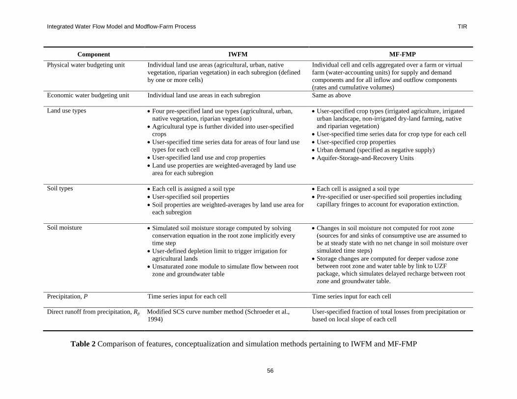
Integrated Water Flow Model and Modflow-Farm Process TIR
56
Component IWFM MF-FMP Physical water budgeting unit Individual land use areas (agricultural, urban, native
vegetation, riparian vegetation) in each subregion (defined by one or more cells)
Individual cell and cells aggregated over a farm or virtual farm (water-accounting units) for supply and demand components and for all inflow and outflow components (rates and cumulative volumes)
Economic water budgeting unit Individual land use areas in each subregion
Same as above
Land use types • Four pre-specified land use types (agricultural, urban, native vegetation, riparian vegetation)
• Agricultural type is further divided into user-specified crops
• User-specified time series data for areas of four land use types for each cell
• User-specified land use and crop properties • Land use properties are weighted-averaged by land use
area for each subregion
• User-specified crop types (irrigated agriculture, irrigated urban landscape, non-irrigated dry-land farming, native and riparian vegetation)
• User-specified time series data for crop type for each cell • User-specified crop properties • Urban demand (specified as negative supply) • Aquifer-Storage-and-Recovery Units
Soil types • Each cell is assigned a soil type • User-specified soil properties • Soil properties are weighted-averages by land use area for
each subregion
• Each cell is assigned a soil type • Pre-specified or user-specified soil properties including
capillary fringes to account for evaporation extinction.
Soil moisture • Simulated soil moisture storage computed by solving conservation equation in the root zone implicitly every time step
• User-defined depletion limit to trigger irrigation for agricultural lands
• Unsaturated zone module to simulate flow between root zone and groundwater table
• Changes in soil moisture not computed for root zone (sources for and sinks of consumptive use are assumed to be at steady state with no net change in soil moisture over simulated time steps)
• Storage changes are computed for deeper vadose zone between root zone and water table by link to UZF package, which simulates delayed recharge between root zone and groundwater table.
Precipitation, P Time series input for each cell
Time series input for each cell
Direct runoff from precipitation, Rp
Modified SCS curve number method (Schroeder et al., 1994)
User-specified fraction of total losses from precipitation or based on local slope of each cell
Table 2 Comparison of features, conceptualization and simulation methods pertaining to IWFM and MF-FMP

Integrated Water Flow Model and Modflow-Farm Process TIR
57
Component IWFM MF-FMP
Irrigation water, I • Used only for urban and agricultural areas • User-specified or calculated for a subregion based on
input data for precipitation, ETc-pot, return flow and re-use fractions, and dynamically updated soil moisture in the root zone.
• Used only for urban and agricultural areas • Calculated for each cell, on an iterative level, and based
on a dynamically updated groundwater head-dependent evapotranspirative crop irrigation requirement
Irrigation efficiency, e • Not specified explicitly; instead specified in terms of
return flow and re-use factors as a fraction of total irrigation water
• User-defined for each farm and crop • Dynamic efficiency based on conservation water use
Irrigation return flow, Ri • Initial return flow is computed as a fraction of irrigation water
• Net return flow is computed as initial return flow less re-use of irrigation water
• User-specified fraction of total losses from irrigation • User-specified fate of return flow of excess imported
water to stream network or injection into farm wells • Semi-routed return flows to stream network facilitate the
simulation of extensive drain networks and lined canals Surface water deliveries • Deliveries can be imported from outside the model area
• Specified or computed deliveries originating from user-specified stream segments
• Some or all deliveries can be dynamically adjusted to meet the water demand; however, deliveries originating from modeled stream nodes are limited by available in-stream flows
• Non-routed Deliveries (unlimited number of ranked water market components)
• Semi-routed Deliveries (linkage to SFR package stream network and simulated diversion points) with no simulation of routed conveyance between diversion points and farm.
• Fully-Routed Deliveries (linkage to SFR package) with simulation of routed conveyance to the farm.
• All deliveries are demand-driven but supply constrained Surface water appropriations • All deliveries have equal priority • User-defined equal appropriation or prior appropriation
• Prior appropriation ranked by farm number for priority of surface water right deliveries
Groundwater pumpage • Well pumping (individual wells are simulated) or element pumping (cluster of wells are simulated)
• Lumped pumping can be distributed to individual wells/elements based on user-specified fractions
• Pumping at a well and element is distributed to aquifer layers using Kozeny equation and user-specified fractions, respectively
• Pumping can be exported outside a subregion • Pumping is limited by the amount of groundwater storage
at the well location
• Single-aquifer farm wells pumpage based on fraction of total pumping capacity of all wells associated with a farm
• Multi-aquifer farm wells linked to MNW package • Wells associated with Farm but not limited to Farm
domain • Series of ranked well fields can export water to individual
farms, which import this water as simulated non-routed deliveries (WELLFIELD option)
Table 2 (continued) Comparison of features, conceptualization and simulation methods pertaining to IWFM and MF-FMP
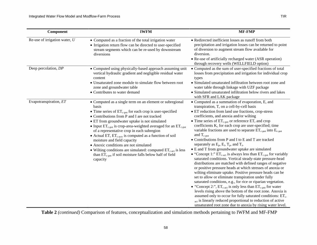
Integrated Water Flow Model and Modflow-Farm Process TIR
58
Component IWFM MF-FMP
Re-use of irrigation water, U
• Computed as a fraction of the total irrigation water • Irrigation return flow can be directed to user-specified
stream segments which can be re-used by downstream diversions
• Redirected inefficient losses as runoff from both precipitation and irrigation losses can be returned to point of diversion to augment stream flow available for diversion.
• Re-use of artificially recharged water (ASR operation) through recovery wells (WELLFIELD option)
Deep percolation, DP • Computed using physically-based approach assuming unit vertical hydraulic gradient and negligible residual water content
• Unsaturated zone module to simulate flow between root zone and groundwater table
• Contributes to water demand
• Computed as the sum of user-specified fractions of total losses from precipitation and irrigation for individual crop types
• Simulated unsaturated infiltration between root zone and water table through linkage with UZF package
• Simulated unsaturated infiltration below rivers and lakes with SFR and LAK package
Evapotranspiration, ET • Computed as a single term on an element or subregional basis
• Time series of ETc-pot for each crop is user-specified • Contributions from P and I are not tracked • ET from groundwater uptake is not simulated • Input ETc-pot is crop-area-weighted averaged for an ETc-pot
of a representative crop in each subregion • Actual ET, ETc-act, is computed as a function of soil
moisture and field capacity • Anoxic conditions are not simulated • Wilting conditions are simulated: computed ETc-act is less
than ETc-pot if soil moisture falls below half of field capacity
• Computed as a summation of evaporation, E, and transpiration, T, on a cell-by-cell basis
• ET reduction from land use fractions, crop-stress coefficients, and anoxia and/or wilting
• Time series of ETc-pot or reference ETr and crop coefficients Kc for each crop are user-specified; time variable fractions are used to separate ETc-pot into Ec-pot and Tc-pot
• Contributions from P and I to E and T are tracked separately as Ep, Ei, Tp, and Ti,
• E and T from groundwater uptake are simulated • “Concept 1:” ETc-act is always less than ETc-pot for variably
saturated conditions. Vertical steady-state pressure-head distributions are matched with defined ranges of negative or positive pressure heads at which stresses of anoxia or wilting eliminate uptake. Positive pressure heads can be set to allow or eliminate transpiration under fully saturated conditions, e.g., for rice or riparian vegetation.
• “Concept 2:”, ETc-act is only less than ETc-pot for water levels rising above the bottom of the root zone. Anoxia is assumed only to occur for fully saturated conditions: ETc-
act is linearly reduced proportional to reduction of active unsaturated root zone due to anoxia by rising water level.
Table 2 (continued) Comparison of features, conceptualization and simulation methods pertaining to IWFM and MF-FMP
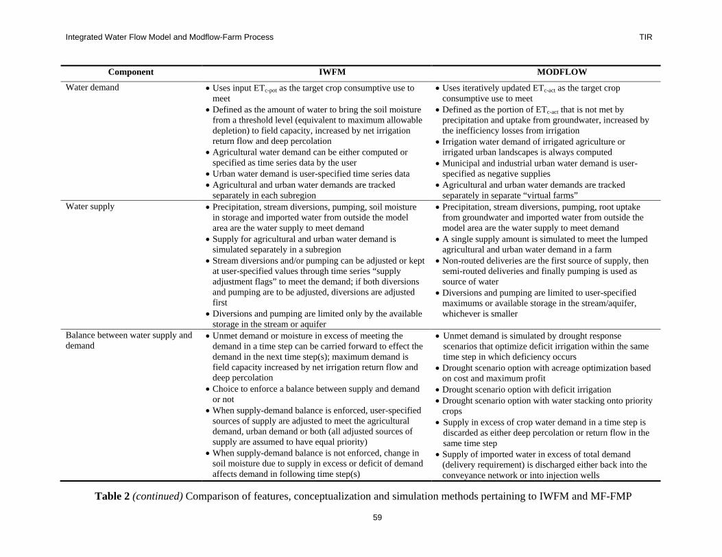
Integrated Water Flow Model and Modflow-Farm Process TIR
59
Component IWFM MODFLOW
Water demand • Uses input ETc-pot as the target crop consumptive use to meet
• Defined as the amount of water to bring the soil moisture from a threshold level (equivalent to maximum allowable depletion) to field capacity, increased by net irrigation return flow and deep percolation
• Agricultural water demand can be either computed or specified as time series data by the user
• Urban water demand is user-specified time series data • Agricultural and urban water demands are tracked
separately in each subregion
• Uses iteratively updated ETc-act as the target crop consumptive use to meet
• Defined as the portion of ETc-act that is not met by precipitation and uptake from groundwater, increased by the inefficiency losses from irrigation
• Irrigation water demand of irrigated agriculture or irrigated urban landscapes is always computed
• Municipal and industrial urban water demand is user-specified as negative supplies
• Agricultural and urban water demands are tracked separately in separate “virtual farms”
Water supply • Precipitation, stream diversions, pumping, soil moisture in storage and imported water from outside the model area are the water supply to meet demand
• Supply for agricultural and urban water demand is simulated separately in a subregion
• Stream diversions and/or pumping can be adjusted or kept at user-specified values through time series “supply adjustment flags” to meet the demand; if both diversions and pumping are to be adjusted, diversions are adjusted first
• Diversions and pumping are limited only by the available storage in the stream or aquifer
• Precipitation, stream diversions, pumping, root uptake from groundwater and imported water from outside the model area are the water supply to meet demand
• A single supply amount is simulated to meet the lumped agricultural and urban water demand in a farm
• Non-routed deliveries are the first source of supply, then semi-routed deliveries and finally pumping is used as source of water
• Diversions and pumping are limited to user-specified maximums or available storage in the stream/aquifer, whichever is smaller
Balance between water supply and demand
• Unmet demand or moisture in excess of meeting the demand in a time step can be carried forward to effect the demand in the next time step(s); maximum demand is field capacity increased by net irrigation return flow and deep percolation
• Choice to enforce a balance between supply and demand or not
• When supply-demand balance is enforced, user-specified sources of supply are adjusted to meet the agricultural demand, urban demand or both (all adjusted sources of supply are assumed to have equal priority)
• When supply-demand balance is not enforced, change in soil moisture due to supply in excess or deficit of demand affects demand in following time step(s)
• Unmet demand is simulated by drought response scenarios that optimize deficit irrigation within the same time step in which deficiency occurs
• Drought scenario option with acreage optimization based on cost and maximum profit
• Drought scenario option with deficit irrigation • Drought scenario option with water stacking onto priority
crops • Supply in excess of crop water demand in a time step is
discarded as either deep percolation or return flow in the same time step
• Supply of imported water in excess of total demand (delivery requirement) is discharged either back into the conveyance network or into injection wells
Table 2 (continued) Comparison of features, conceptualization and simulation methods pertaining to IWFM and MF-FMP

Integrated Water Flow Model and Modflow-Farm Process TIR
60
Appendix A: Notation
The following symbols are used in this report:
a = anoxia fringe;
c = capillary fringe;
CIR = crop irrigation requirement;
CN = curve number;
d = thickness of stream bed material;
DP = deep perco0lation that leaves the root zone as the moisture moves downward;
e = on-farm efficiency defined as the fraction of the total irrigation water that is
used beneficially in the farm;
Ec-act = actual evaporation;
Ec-pot = potential crop evaporation;
Ei-act = actual evaporation from irrigation;
Ei-pot = potential evaporation from irrigation;
Ep-pot = potential evaporation from precipitation;
ETc = crop evapotranspiration under standard conditions;
ETc-act = total actual crop evapotranspiration;
ETc-adj = crop evapotranspiration under non-standard conditions;
ETc-pot = potential crop evapotranspiration;
ETgw-act = root uptake from groundwater;
ETi-act = portion of actual evapotranspiration fed by irrigation;
ETp-act = portion of actual evapotranspiration fed by precipitation;
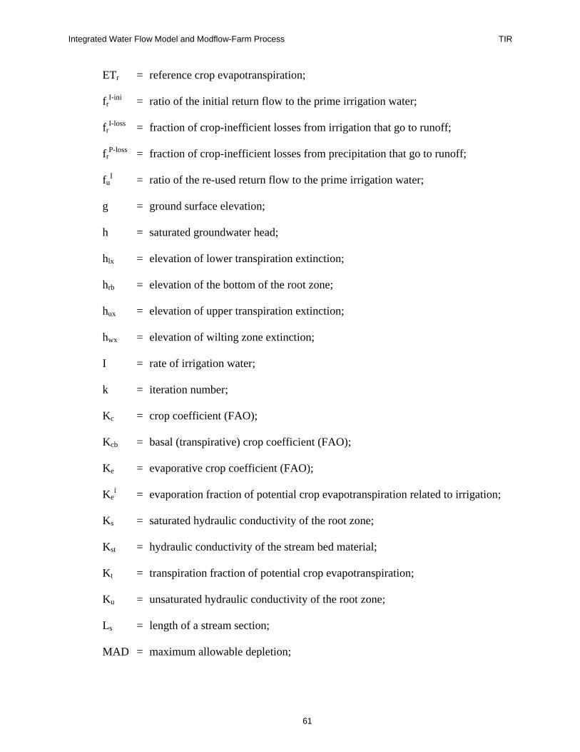
Integrated Water Flow Model and Modflow-Farm Process TIR
61
ETr = reference crop evapotranspiration;
frI-ini = ratio of the initial return flow to the prime irrigation water;
frI-loss = fraction of crop-inefficient losses from irrigation that go to runoff;
frP-loss = fraction of crop-inefficient losses from precipitation that go to runoff;
fuI = ratio of the re-used return flow to the prime irrigation water;
g = ground surface elevation;
h = saturated groundwater head;
hlx = elevation of lower transpiration extinction;
hrb = elevation of the bottom of the root zone;
hux = elevation of upper transpiration extinction;
hwx = elevation of wilting zone extinction;
I = rate of irrigation water;
k = iteration number;
Kc = crop coefficient (FAO);
Kcb = basal (transpirative) crop coefficient (FAO);
Ke = evaporative crop coefficient (FAO);
Kei = evaporation fraction of potential crop evapotranspiration related to irrigation;
Ks = saturated hydraulic conductivity of the root zone;
Kst = hydraulic conductivity of the stream bed material;
Kt = transpiration fraction of potential crop evapotranspiration;
Ku = unsaturated hydraulic conductivity of the root zone;
Ls = length of a stream section;
MAD = maximum allowable depletion;
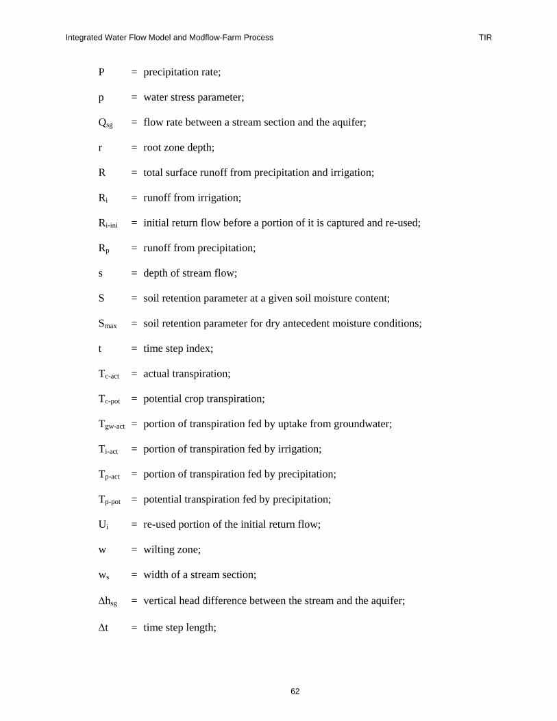
Integrated Water Flow Model and Modflow-Farm Process TIR
62
P = precipitation rate;
p = water stress parameter;
Qsg = flow rate between a stream section and the aquifer;
r = root zone depth;
R = total surface runoff from precipitation and irrigation;
Ri = runoff from irrigation;
Ri-ini = initial return flow before a portion of it is captured and re-used;
Rp = runoff from precipitation;
s = depth of stream flow;
S = soil retention parameter at a given soil moisture content;
Smax = soil retention parameter for dry antecedent moisture conditions;
t = time step index;
Tc-act = actual transpiration;
Tc-pot = potential crop transpiration;
Tgw-act = portion of transpiration fed by uptake from groundwater;
Ti-act = portion of transpiration fed by irrigation;
Tp-act = portion of transpiration fed by precipitation;
Tp-pot = potential transpiration fed by precipitation;
Ui = re-used portion of the initial return flow;
w = wilting zone;
ws = width of a stream section;
∆hsg = vertical head difference between the stream and the aquifer;
∆t = time step length;

Integrated Water Flow Model and Modflow-Farm Process TIR
63
ηT = total porosity;
λ = pore size distribution index;
θ = soil moisture in the root zone;
θf = field capacity.
Integrated Water Flow Model and Modflow-Farm Process TIR
64
References
Allen, RG; Pereira, LS; Raes, D; Smith, M. 1998. Crop evapotranspiration - Guidelines for computing crop water requirements. Rome: Food and Agriculture Organization of the United Nations. 300 p. Irrigation and Drainage Paper 56.
Brush, CF; Dogrul, EC; Moncrief, M; Galef, J; Shultz, S; Tonkin, M; Wendell, D;
Kadir, T; Chung, F. 2008. Estimating hydrologic flow components of the Central Valley hydrologic flow system with the California Central Valley Groundwater-Surface water Model. In: Brush, CF; Miller, NL, editors. Proceedings of the California Central Valley Groundwater Modeling Workshop. July 10-11, 2008; Lawrence Berkeley National Laboratory, Berkeley, (CA). Sacramento (CA): California Water and Environmental Modeling Forum. p. 80-88.
[BCDWRC]. Butte County Department of Water and Resource Conservation.
2008a. Butte Basin groundwater model update: Phase II report. [Internet]. Butte County Department of Water and Resource Conservation. variously paged. Technical memorandum, March 2008. [cited: 2008 Dec 18]. Available at: http://www.buttecounty.net/waterandresource/GWModelupdate/BCDWRC%20Model%20TM2%20FINAL.pdf
[BCDWRC]. Butte County Department of Water and Resource Conservation.
2008b. Butte Basin groundwater model update: base case and water management scenerio simulations. [Internet]. Butte County Department of Water and Resource Conservation. variously paged. Technical memorandum, April 2008. [cited: 2008 Dec 18]. Available at: http://www.buttecounty.net/waterandresource/GWModelupdate/TM3%20Base%20Case%20-%20Scenario%2020080424.pdf
[CADWR]. California Department of Water Resources. 1998. California Water
Plan. Sacramento (CA): California Department of Water Resources. Bulletin 160. Campbell, GS. 1974. A simple method for determining unsaturated hydraulic
conductivity from moisture retention data. Soil Sci. 117(6):311-314. CWEMF, 2008, Central Valley Groundwater Modeling Workshop, California
Water Environmental Modeling Forum, [Internet]. [cited: 2008 Sept 11]. Available at: http://www.cwemf.org/workshops/GWWorkshop/
[DHI]. Danish Hydraulic Institute. 1999. MIKE SHE Pre- and Post-Processing
User Manual. Hørsholm, Denmark: DHI Software. Dogrul, EC. 2009a. Integrated Water Flow Model (IWFM v3.1): Theoretical
documentation. Sacramento (CA): Integrated Hydrological Models Development Unit,
Integrated Water Flow Model and Modflow-Farm Process TIR
65
Modeling Support Branch, Bay-Delta Office, California Department of Water Resources. variously paged.
Dogrul, EC. 2009b. Integrated Water Flow Model (IWFM v3.1): User’s manual.
Sacramento (CA): Integrated Hydrological Models Development Unit, Modeling Support Branch, Bay-Delta Office, California Department of Water Resources. variously paged.
Drew, MC. 1997, Oxygen deficiency and root metabolism. Injury and acclimation
under hypoxia and anoxia. Annual Rev. Plant Physiol. Plant Mol. Biol. 1997. 48:223–250.
Driscoll, FG. 1986. Groundwater and wells. 2nd ed. St. Paul (MN): Johnson Division. 1089 p.
Faunt, CC; Belitz, K; Hanson, RT. 2009b. Chapter B: Groundwater availability in
California’s Central Valley. (Faunt, CC, editor. Groundwater availability of the Central Valley aquifer of California). Reston (VA): US Geological Survey. 225 p. Professional Paper 1766.
Faunt, CC; Hanson, RT; Belitz, K. 2009a. Chapter A: Introduction, overview of
hydrology, and textural model of California’s Central Valley. (Faunt, CC, editor. Groundwater availability of the Central Valley aquifer of California). Reston (VA): US Geological Survey. 225 p. Professional Paper 1766.
Faunt, CC; Hanson, RT; Belitz, K; Schmid, W; Predmore, SP; Rewis, D L;
McPherson, K. 2009c. Chapter C: Numerical model of the hydrologic landscape and groundwater flow in California’s Central Valley. (Faunt, CC, editor. Groundwater availability of the Central Valley aquifer of California). Reston (VA): US Geological Survey. 225 p. Professional Paper 1766.
Faunt, CC; Hanson, RT; Schmid, W; Belitz, K. 2008. Applying MODFLOW's
Farm Process to California's Central Valley. In: Brush, CF; Miller, NL, editors. Proceedings of the California Central Valley Groundwater Modeling Workshop. July 10-11, 2008; Lawrence Berkeley National Laboratory, Berkeley (CA). Sacramento (CA): California Water and Environmental Modeling Forum. p. 78-80.
Feddes, R.A., Kowalik, P., Kolinska-Malinka, K. and H. Zaradny, 1976,
Simulation of field water uptake by plants using a soil water dependent root extraction function, Journal of Hydrolology 31 (1976), pp. 13–26.
Guan, H. and J.L. Wilson, 2009, A hybrid dual-source model for potential
evaporation and transpiration partitioning, Journal of Hydrology 377 (2009) 405–416. Halford, KJ; Hanson, RT. 2002. User’s guide for the drawdown-limited, multi-
node well (MNW) package for the U. S. Geologic Survey’s modular three-dimensional finite-difference groundwater flow model, versions MODFLOW-96 and MODFLOW-2000. Sacramento (CA): US Geological Survey. 33 p. Open-File Report 02-293.
Integrated Water Flow Model and Modflow-Farm Process TIR
66
Available at: http://pubs.usgs.gov/of/2002/ofr02293/text.html Hanson, RT; Martin, P; Koczot, KM. 2003. Simulation of groundwater/surface
water flow in the Santa Clara - Calleguas basin, California. Sacramento (CA): US Geological Survey. 214 p. Water Resources Investigations Report 02-4136. Available at: http://water.usgs.gov/pubs/wri/wri024136/text.html
Hanson, RT; Schmid, W; Lear, WJ; Faunt, CC. 2008. Simulation of an Aquifer-
Storage-and-Recovery (ASR) System using the Farm Process in MODFLOW for the Pajaro Valley, Monterey Bay, California. In: Poeter, E; Hill, M; Zheng, C, editors. Modflow and More 2008: Groundwater and Public Policy. May 18-21, 2008; International Groundwater Modeling Center. Golden (CO): Colorado School of Mines. p. 501-505.
Hanson, R.T., Schmid, Wolfgang, Faunt, C.C., and Lockwood, B., 2010, Simulation and Analysis of Conjunctive Use with MODFLOW's Farm Process: Ground Water Vol. 48, No. 5, pp. 674 - 689.( DOI: 10.1111/j.1745-6584.2010.00730.x)
Harbaugh, AW. 2005. MODFLOW-2005, the US Geological Survey modular
groundwater model-the Ground-water Flow Process. Reston (VA): US Geological Survey. variously paged. Techniques and Methods 6-A16.
Harbaugh, AW; Banta, E R; Hill, MC; McDonald, MG. 2000. MODFLOW-2000,
the US Geological Survey modular ground-water model-User guide to modularization concepts and the Groundwater Flow Process. Reston (VA): US Geological Survey. 121 p. Open-File Report 00-92.
Illangasekare, T. 2001. MIKE SHE code verification and validation for RFETS
site-wide water balance model. [Internet]. Prepared by Colorado School of Mines, Golden, Colorado in collaboration with Robert Prucha, RMC Consultants and DHI-Water and Environment for Kaiser-Hill Company, L.L.C. 28 p. September 28, 2001. [cited: 2008 Oct 4]. Available at: http://www.integratedhydro.com/MSHEVerification_summary.pdf
Jimenez, ACP. 2008. Modeling surface water and groundwater interactions near
Milton-Freewater, Oregon. [master's thesis]. [Corvalis (OR)]: Department of BioResource Engineering, Oregon State University. 105 p.
Kavvas, ML; Chen, ZQ; Dogrul, C; Yoon, JY; Ohara, N; Liang, L; Aksoy, H;
Anderson, ML; Yoshitani, J; Fukami, K; Matsuura, T. 2004. Watershed Environmental Hydrology (WEHY) model based on upscaled conservation equations: hydrologic module. J. Hydrol. Engrng. 9(6):450-464.
Kim, NW; Chung, IM; Won, YS; Arnold, JG. 2008. Development and application
of the integrated SWAT–MODFLOW model. J. Hydrol. 356(1-2):1-16. Kollet, SJ; Maxwell, RM. 2008. Capturing the influence of groundwater dynamics
Integrated Water Flow Model and Modflow-Farm Process TIR
67
on land surface processes using an integrated, distributed watershed model. Water Resour. Res. 44: W02402.
Kroes, J.G. and J.C. van Dam (eds), 2003. Reference Manual SWAP version
3.0.4. Wageningen, Alterra, Green World Research.. Alterra-report 773. Reference Manual SWAP version 3.0.4.doc. 211 pp
Kustas, W.P., Norman, J.M., 1997. A two-source approach for estimating
turbulent fluxes using multiple angle thermal infrared observations. Water Resources Research 33 (6), 1495–1508.
Leavesley, GH; Lichty, RW; Troutman, BM; Saindon, LG. 1983. Precipitation-
Runoff Modeling System: User's Manual. Denver (CO): US Geological Survey. 207 p. Water Resources Investigations Report 83-4238.
Markstrom, SL; Niswonger, RG; Regan, RS; Prudic, DE; Barlow, PM. 2008.
GSFLOW--Coupled Groundwater and Surface water FLOW model based on the integration of the Precipitation-Runoff Modeling System (PRMS) and the Modular Groundwater Flow Model (MODFLOW-2005). Reston (VA): US Geological Survey. 240 p. Techniques and Methods 6-D1.
Mathur, S. and S. Rao, 1999, Modeling Water Uptake by Plant Roots, Journal of
Irrigation and Drainage Engineering, Vol. 125, No. 3, May/June 1999, pp. 159-165. Maxwell, RM; Miller, NL. 2005. Development of a coupled land surface and
groundwater model. J. Hydrometeorol. 6(3): 233-247. McDonald, MG; Harbaugh, AW. 1988. A modular three-dimensional finite-
difference groundwater flow model. (US Geologic Survey Technical Water Resources Investigation; Book 6). Reston (VA): US Geological Survey. Ch. A1. Techniques of Water-Resource Investigation 6-A1.
Miller, NL; Dale, LL; Brush, CF; Vicuna, SD; Kadir, TN; Dogrul, EC; Chung, FI.
2009. Drought resilience of the California Central Valley surface-groundwater-conveyance system. J. Am. Water Resour. Assn. 45(4):857-866.
[MW]. Montgomery Watson. 1993. Documentation and user’s manual for
integrated groundwater and surface water model. Sacramento (CA): Montgomery Watson. variously paged.
Niswonger, RG; Prudic, DE. 2005. Documentation of the Stream flow-Routing
(SFR2) Package to include unsaturated flow beneath streams-A modification to SFR1. Reston (VA): US Geological Survey. 57 p. Techniques and Methods 6-A13.
Niswonger, RG; Prudic, DE; Regan, RS. 2006. Documentation of the
Unsaturated-Zone Flow (UZF1) Package for modeling unsaturated flow between the
Integrated Water Flow Model and Modflow-Farm Process TIR
68
land surface and the water table with MODFLOW-2005. Reston (VA): US Geological Survey. 62 p. Techniques and Methods 6-A19.
Prasad, R. 1988. ‘‘A linear root water uptake model.’’ Journal of Hydrology, 99,
297–306. Prickett, TA; Lonnquist, CG. 1971. Selected Digital Computer Techniques for
Groundwater Resource Evaluation. Urbana (IL): Illinois State Water Survey. 62 p. Bulletin 55. Available at: http://www.isws.illinois.edu/pubdoc/B/ISWSB-55.pdf
Prucha, RH. 2004. Review of MIKESHE. Southwest Hydrology.
January/February:37. Prudic, DE; Konikow, LF; Banta, ER. 2004. A new stream-flow routing (SFR1)
package to simulate stream-aquifer interaction with MODFLOW-2000. Carson City (NV): US Geological Survey. 104 p. Open-File Report 2004-1042.
Said, A; Steven, DK; Sehlke, G. 2005. Estimating water budget in a regional
aquifer using HSPF-MODFLOW Integrated Model. J. Am. Water Resour. As. 41(1):55-66.
Schmid, W. 2004. A Farm Package for MODFLOW-2000: Simulation of Irrigation
Demand and Conjunctively Managed Surface water and Groundwater Supply. [dissertation]. [Tucson (AZ)]: Department of Hydrology and Water Resources, The University of Arizona. 278 p.
Schmid, W; Dogrul, EC; Hanson, RT; Kadir, T; Chung, F. 2011. Comparison of
simulations of land-use specific water demand and irrigation water supply by MF-FMP and IWFM, California Department of Water Resources Technical Information Report No. xx, xxxp.
Schmid, W; Hanson, RT. 2009a. Appendix 1: Supplemental Information –
Modifications to MODFLOW-2000 packages and processes. (Faunt, CC, editor. Groundwater availability of the Central Valley aquifer of California). Reston (VA): US Geological Survey. 225 p. US Geological Survey Professional Paper 1766.
Schmid, W; Hanson, RT. 2009b. The Farm Process Version 2 (FMP2) for
MODFLOW-2005 - modifications and upgrades of FMP1 and inclusion into MODFLOW-2005. (Book 6). Reston (VA): US Geological Survey. 102 p. Techniques and Methods 6-A32.
Schmid, W., J.P. King, and T.M. Maddock III. 2009c. Conjunctive Surface-
water/groundwater model in the southern Rincon Valley using MODFLOW-2005 with the Farm Process: New Mexico Water Resources Research Institute Completion Report No. 350.
Integrated Water Flow Model and Modflow-Farm Process TIR
69
Schmid, W; Hanson, RT; Maddock III, T; Leake, SA. 2006. User guide for the farm process (FMP1) for the US Geological Survey’s modular three-dimensional finite-difference groundwater flow model, MODFLOW-2000. (Book 6). Reston (VA): US Geological Survey. 127 p. Techniques and Methods 6-A17. Available at: http://pubs.usgs.gov/tm/2006/tm6A17/
Schroeder, PR; Dozier, TS; Zappi, PA; McEnroe, BM; Sjostrom, JW; Peton, RL.
1994. The hydrologic evaluation of landfill performance (HELP) model: engineering documentation for version 3. Washington (DC): US Environmental Protection Agency, Office of Research and Development. 84 p. EPA/600/R-94/168b.
Schwankl, LJ; Prichard, TL; Hanson, BR. 2008. Reducing runoff from irrigated
lands, tailwater return systems. [Internet]. University of California, Division of Agricultural and Natural Resources. Publication 8225. [cited: 2008 Aug 27]. Available at: http://anrcatalog.ucdavis.edu/pdf/8225.pdf
Shuttleworth, W.J., Wallace, J.S., 1985. Evaporation from sparse crops – an
energy combination theory. Quarterly Journal of the Royal Meteorological Society 111. Simunek, J; Sejna, M; van Genuchten, MT. 1999. HYDRUS-2D/MESHGEN-2D.
Simulating water flow and solute transport in two-dimensional variably saturated media. Golden (CO): Colorado School of Mines. 227 p. Handbook, International Groundwater Modeling Center – TPS 53C, Version 2.0.
Sophocleous, MA; Koelliker, JK; Govindaraju, RS; Birdie, T; Ramireddygari, SR;
Perkins, SP. 1999. Integrated numerical modeling for basin-wide water management – The case of the Rattlesnake Creek Bain in South-central Kansas. J. Hydrol. 214(1-4):179-196.
Sophocleous, MA; Perkins, SP. 2000. Methodology and application of combined
watershed and groundwater models in Kansas. J. Hydrol. 236(3-4):185-201. Synder, R; Orang, M; Geng, S; Matyac, S; Sarreshteh, S. 2005. SIMETAW
(Simulation of Evapotranspiration of Applied Water). (California Water Plan Update 2005; vol. 4: reference guide). Sacramento (CA): California Department of Water Resources.
Therrien, R.; McLaren, R.G., Sudicky, E.A. 2007. HydroGeoSphere—a three-
dimensional numerical model describing fully-integrated subsurface and surface flow and solute transport (Draft). Groundwater Simulations Group, University of Waterloo.
USDA, Soil Conservation Service. 1985. National engineering handbook.
Washington (DC): US Department of Agriculture. Section 4, Hydrology, Chapters 9 and 10.
Williamson, AK; Prudic, DP; Swain, LW. 1989. Ground-water flow in the Central

Integrated Water Flow Model and Modflow-Farm Process TIR
70
Valley, California. Washington (DC): US Geological Survey. variously paged. Professional Paper 1401-D.
Yoon, YS. 1976. Identification of aquifer parameters in a large unconfined
system: with finite elements and constrained nonlinear least squares optimization. [dissertation]. [Los Angeles]: Department of Civil and Environmental Engineering, University of California.