Comparison of methods for harmonic wavelet analysis of heart rate variability

1

R.A. Bates M.F.Hilton K.R.Godfrey M.J.Chappell

Indexing terms: Biomedical engineering, Harmonic wavelet analysis

Abstract: Two different methods for the spectral analysis of heart rate variability data are compared: the discrete Fourier transform and the nonequispaced Fourier transform. The methods are used to analyse test signals that are constructed to mimic R-R interval data, with graded levels of noise, generated using the integral pulse frequency modulation model. It is found that the nonequispaced Fourier transform is the better method for determining the frequency coefficients of the test signals as the noise level is increased. Both methods are compared when they are used as the first step in a time-frequency analysis of the test signals using the discrete harmonic wavelet transform, and a quantitative comparison is made on a set of randomly generated test signals (this shows that the nonequispaced Fourier transform is the better method). A further study shows the ability of the discrete harmonic wavelet transform to detect frequencies close to the boundary between wavelet levels. Since each harmonic wavelet represents a distinct frequency band, careful choice of sampling frequency means that such wavelets can be used to identify spectral bands associated with physiological causes. A clinical example, using the nonequispaced Fourier transform, shows how the discrete harmonic wavelet transform could be developed for use in detecting brief alterations in autonomic tone.

1 Introduction

The aim of this paper is to compare two different methods of computing the Fourier coefficients of a nonequispaced time series when used as the first step in a time-frequency analysis of heart rate variability using the discrete harmonic wavelet transform (DHWT) [l].

Spectral analysis of heart rate variability is used to quantify autonomic function [2] and aids in the diagno- 0 IEE, 1998 ZEE Proceedings online no. 19982321 Paper first received 28th January and in revised form 28th August 1998 R.A. Bates, M.J. Chappell and K.R. Godfrey are with the Department of Engineering, University of Warwick, Coventry, CV4 7AL, UK M.F. Hilton is with the Department of Respiratory Physiology, Binning- ham Heartlands Hospital, Birmingham, B9 5SS, UK

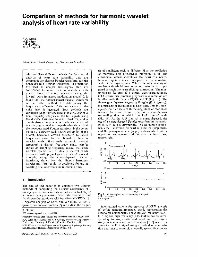
sis of conditions such as diabetes [ 3 ] or the prediction of mortality post myocardial infarction [4, 51. The autonomic system modulates the heart via neuro- humeral inputs which are integrated in the sino-atrial node of the myocardium. When this integrated signal reaches a threshold level an action potential is propa- gated through the heart eliciting contraction. The mor- phological features of a typical electrocardiographic (ECG) waveform producing myocardial contraction are labelled with the letters PQRS and T (Fig. la). The time elapsed between successive R peaks (R-R interval) is a measure of instantaneous heart rate. This is a non- equispaced time series with the magnitude of each R-R interval plotted on the y-axis, the x-axis being the cor- responding time at which the R-R interval ends (Fig. Ib). As the R-R interval is nonequispaced, the use of a nonequispaced Fourier transform in the analy- sis of R-R data is appropriate. The autonomic compo- nents that determine the heart rate are the sympathetic and the parasympathetic (vagal) systems which act in opposition to increase and decrease the heart rate, respectively.

1.0 R<---,R 1

01 ' 0 0.5 1.0 1.5 2.0 2.5 3.0 3.5 4.0

time, s Fig. 1 a ECG waveform b RR signal

ECG waveform and corresponding RR signal

International criteria for practices of HRV analysis [6] define standard frequency bands representing the autonomic components. These are low frequency (0.04- 0.15Hz) and high frequency (0.15-0.4Hz) power, corre- sponding to sympathetic and vagal activity, respec- tively. A common method of analysis [2, 71 is to fit a curve to the R-R signal using a method of interpola- tion and then to resample at equally spaced time points

291 IEE Proc-Sci. Meas. Technol., Vol. 145, No. 6, November 1998

to obtain a regular time series. Fourier transforms can then be used to obtain the power spectrum over the full length of the series, recommended to be not less than 5min [6]. This provides information on the frequency content of the signal with a fixed resolution in time and frequency. Some pathologies involve transient altera- tions in autonomic tone and may benefit from analysis with improved time resolution. Obstructive sleep apnoea (OSA) is a condition where respiration during sleep is punctuated with repetitive cyclical pauses [8], producing transient autonomic alterations at cycles between 14 and 90s. Quantification of these transients may provide a mechanism for the association between OSA and cardiovascular disease 19, 101. It is in this context that time-frequency analysis may provide a useful method of mapping autonomic abnormalities (see, for example, [ll]).

In this paper the method outlined above using the DFT is compared with the nonequispaced Fourier transform (NeFT) method. The ability of both methods to deal with noisy signals is investigated using a test signal with Gaussian white noise added. The test signal is developed using the integral pulse frequency modula- tion (IPFM) model [12]. In addition, both methods are used as the first step in an analysis using the discrete harmonic wavelet transform (the methodology of which is described in 111, Chap. 17, pp. 364-369) to provide better time resolution than spectral analysis using the DFT.

The advantage of using harmonic wavelets in this case, over wavelets formed from dilation equations, is that each level of the DHWT represents a distinct fre- quency band [l, 131. Thus, by choosing an appropriate series length and sampling rate, the spectral frequency bands recommended [6] can be adhered to, maintaining the physiological significance of results. This property is not offered by continuous wavelet transforms as their reduced frequency resolution produces overlapping fre- quency bands. The benefit of using wavelets over the short time Fourier transform are that less processing of the data is required, there is no need to interpolate the R-R data, overlapping windowed sections are not needed and the DHWT avoids the precondition of sta- tionarity. A comparison of the effectiveness of each method is made using simulated data where the fre- quency components and noise levels are known in advance. In the final part of the paper (Section 5) , the NeFT and DHWT methods are applied to real data collected from a subject at the Sleep Disorders Unit, Birmingham Heartlands Hospital, UK.

2 Methods

In this paper two methods are used for the generation of equispaced Fourier coefficients from a nonequis- paced time series. For N data points the series is repre- sented by

(I) 2, = ~ ( t , ) r = 0 , 1 , 2 , . . . , N - 1

2.1 Discrete Fourier transform One solution to the problem of analysing nonequis- paced data is to fit a curve to the data (e.g. using a cubic spline), resample at equispaced points and use the discrete Fourier transform to compute the Fourier coefficients. For N equispaced data points the series { x,} has Fourier coefficients { X,} defined by

292

1 N - l z,e-@"r"/N) XI, = - k = 0 , 1 , 2 , . . . , N - 1

( 2 ) r=O

N

where i = d-1. Eqn. 2 is evaluated using the fast Fou- rier transform [14] when N is a power of 2 (N = 2m, m an integer 2 1).

2.2 Nonequispaced Fourier transform Dutt and Rokhlin [15] presented a group of algorithms which generalised the Fourier transform to deal with noninteger frequencies and nonequispaced data points. The method of computing equispaced frequency coeffi- cients from nonequispaced data points (Problem 1 in [15]) is summarised as

1 N - l X k = ~ , e - ~ ( ~ ~ ~ ~ ~ / ~ ) k = 0 , 1 , 2 , . . . , N - 1

r=O

( 3 ) where t, lies in the interval [-N/2, N/2], x, = x(t,) for r - 0, ..., N - 1. The nonequispaced nature of the time series does not provide an orthogonal basis for calcula- tion of the Fourier coefficients. To compute the Fourier coefficients the x,s are interpolated to the nodes of an integer grid (the time-frequency grid). In this implementation we follow the procedure employed in [15], where the grid is chosen to be 2N square, each e-z(2zkfr'w term is approximated by a 10-term Fourier series, and each Fourier coefficient is approximated by interpolation of the values at the nearest ten equispaced nodes on the grid. In addition to the standard method, the grid is scaled so that, instead of the frequencies rep- resented by the Fourier coefficients being dependent on the length of the series, the coefficients represent a fixed set of frequencies, equivalent to fixing the sam- pling frequency, which is independent of signal length.

2.3 Discrete harmonic wavelet transform Newland [I] describes a form of wavelet analysis, the discrete harmonic wavelet transform (DHWT), which has the desirable property that the wavelet levels repre- sent nonoverlapping frequency bands and can therefore be used to quantify specific frequency bands identified as having clinical significance. In general a harmonic wavelet at levelj 0' an integer 2 1) translated by k steps of size 1/23?' is defined by

-

for 7r2J 5 w 5 2 ~ 2 3 elsewhere

(4) 1 e--z2wk/23

W(U) = { p The elements of this wavelet family are mutually orthogonal and their coefficients can be computed using the fast Fourier transform. The DHWT coeffi- cients are used to construct a time-frequency map (described in [l]) which shows how the frequency spec- trum evolves with time. For a signal of length N = 2" there are YM + 1 wavelet levels (0, .,., m) with a single coefficient at levels 0 and m and 21-l coefficients at each subsequent levelj = 1, ..., m - 1. The band of frequen- cies fi represented by level j is given by

where is the sampling frequency. As an example of using the DHWT, the spectral

analysis of a simple test signal is described. The signal, which is similar to the R-R test signal described in

IEE Pvoc -Sei Meas Technol. Vol 165, No 6, November 1998

Section 2.4, is the sum of two sinusoids, one at O.1Hz whose amplitude decreases linearly with time, and the other at 0.28Hz whose amplitude increases linearly with time. The equation for the signal is given by

t N - l - t~ tr .(tr) = 1 + a sinwlt, + b- sinwzt, tN-1 tN-1

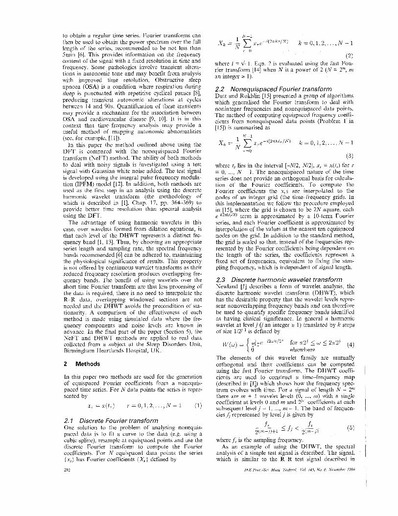
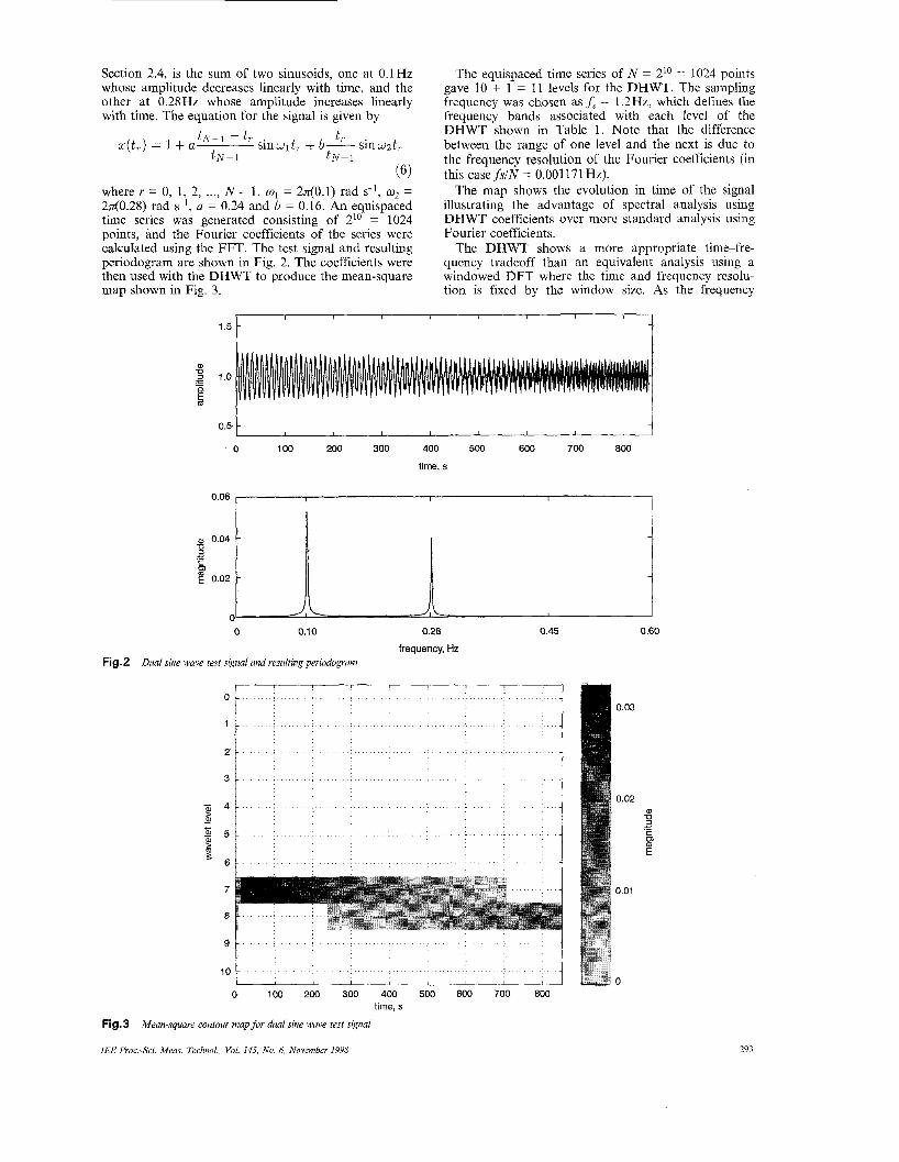
(6) where Y = 0, 1, 2, ..., N - 1, col = 240.1) rad s-l, co2 = 240.28) rad ssl, a = 0.24 and b = 0.16. An equispaced time series was generated consisting of 21° = 1024 points, and the Fourier coefficients of the series were calculated using the FFT. The test signal and resulting periodogram are shown in Fig. 2. The Coefficients were then used with the DHWT to produce the mean-square map shown in Fig. 3 .

The equispaced time series of N = 2'O = 1024 points gave 10 + 1 = 11 levels for the DHWT. The sampling frequency was chosen as f, = 1.2Hz, which defines the frequency bands associated with each level of the DHWT shown in Table 1. Note that the difference between the range of one level and the next is due to the frequency resolution of the Fourier coefficients (in this casefslN = 0.001 171 Hz).

The map shows the evolution in time of the signal illustrating the advantage of spectral analysis using DHWT coefficients over more standard analysis using Fourier coefficients.

The DHWT shows a more appropriate time-fre- quency tradeoff than an equivalent analysis using a windowed DFT where the time and frequency resolu- tion is fixed by the window size. As the frequency

I I I I 5 b I

1.5

0.5 I I I I I I I I

0 1 00 200 300 400 500 600 700 800

time, s

0.06 I I I I

0.10 0.28 0.45 0.60

frequency, Hz Fig.2 Dual sine wave test signal and resulting periodogram

3 t i

'I , . ,.,. ...,..... 1 .. . _ '

7

8 .. ,

' ' i . 1 . ' . .., .,.,.. . * B

10 gB 0 100 200 300 400 500 600 700 800

time, s

0.03

0.02 (U U

c c .-

E 0.01

0

Fig.3 Mean-square contour map for dual sine wave test signal

IEE Proc-Sci. Meas. Technol., Vol. 145, No. 6, November 1998 293

increases, the DHWT analysis provides increasing time resolution and decreasing frequency resolution, defined by the bands represented by the wavelet levels (eqn. 5). The advantage in this application is that analysis of the frequency response is restricted to specific bands known to have physiological significance 161, and these bands are conveniently represented by the different wavelet levels. The time resolution of the analysis is therefore maximised given this restriction.

Table 1: Wavelet level frequency bands for dual sine wave test signal

Level Frequency (Hz)

0 0 (DC) 1 0.001 171

2 0.00234-0.003516

3 0.00468-0.008203

4 0.00937-0.01758

5 0.01875-0.03633

6 0 0375-0.07383

7 0.075-0.1 488

8 0.15-0.2988

9 0.3-0.5988

10 0.6

2.4 R-R test signals The test signals used in this paper to evaluate the per- formance of the different methods are based on the integral pulse frequency modulation (IPFM) model [ 121, which produces a nonequispaced time series simi- lar to the R-R interval data obtained from an ECG analysis. The IPFM model is a physiologically plausible way of developing an event pulse series from known input signals [ 121. Neurohumeral inputs impact on the the sino-atrial (SA) node of the heart and are inte- grated. If this integration exceeds some threshold value the heart spontaneously depolarises; this is represented by the QRS complex of the ECG waveform. The time difference between two consecutive depolarisations is measured as the R-R interval.

We represent two inputs on the SA node as sinusoids of frequencies fi = 0.1 Hz and f i = 0.28 Hz, with ampli- tudes a and b, respectively. These values are chosen so that the two inputs represent a low frequency (LF) input and a high frequency (HF) input, associated with the sympathetic and vagal tones of the autonomic func- tion of the heart, respectively [6]. The signal is derived from the following equation:

T - t . t m(t) = I + a- sinwlt + b- sinwzt + S[ (7) T T

where T represents the duration of the signal in sec- onds, w1 = 2$,, w2 = 2 ~ 5 5 S is a scaling factor and represents noise as an independent random number chosen from a normal distribution with mean zero and variance d. The equation for the IPFM model is

I , = l;+l m ( t ) d t (8)

where 1, represents the value of integration over the interval [t,, t,+l]. If no noise term is present, the analyt- ical solution for eqn. 8 is given by

294

(9) 1 ::I b

w$ T +--(sin w2t - w2t cos wzt)

where t, = rat, r = 0, 1, 2, ... and At is a fixed time interval. If there is noise present, solving eqn. 8 requires special treatment of the noise factor 5 as the expected value of j’ g(t)dt = 0, over any interval. To include the noise term in the formulation of the R-R test signal, eqn. 9 is evaluated from t = 0, with At = 1/128s (see below) and a noise term 5; is added to the value I, obtained. The process is repeated at intervals of At = 1/128s until the sum of the integrals, I, = 2, I,, exceeds the threshold level f, at which point the time of the event is recorded as the nearest sampling interval of the current integration section. I, is then reset to zero and the process repeated until the required number of events have been recorded.

Commercial tape-based ambulatory Holter systems record the ECG at 128Hz, which determines the accu- racy in locating the time of the R peaks in the signal. Choosing an interval At = 1/128s mimics the sampling error of the ECG recorder as this determines the accu- racy in locating the time of an event from the IPFM model.

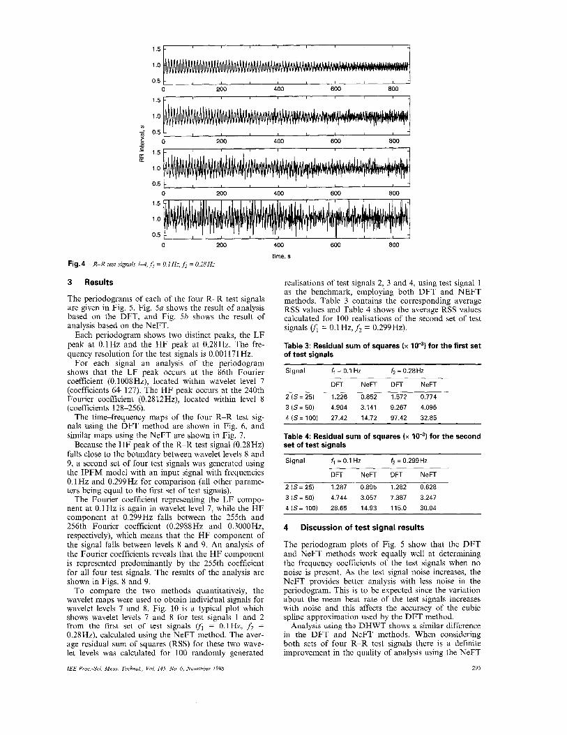
Four different test signals were generated by varying the noise scaling factor S in eqn. 7 with standard devi- ation 0 = 0.0025 (this value in combination with the scaling factors below provides a realistic amount of noise in the generated test signals) and setting a = 0.24, b = 0.16 and 1 = 0.9169. Using these values, a signal was generated which represents an average value of heart rate determined from data collected at Birming- ham Heartlands Hospital from six healthy patients while asleep between the hours of 24:OO and 0S:OO. The four signals were: 1. no noise, S = 0 2. low noise level, S = 25 3. medium noise level, S = 50 4. high noise level, S = 100.

Table 2 shows a summary of the four test signals shown in Fig. 4. For Method A (DFT) it is necessary to fit a cubic spline to each signal and resample at f, = 1.2Hz to obtain an equispaced series. For Method B the scaling of the Fourier coefficients provides an equispaced series with an equivalent sampling fre- quency off , = 1.2Hz.

Table 2: R-R test signal data

R-R signal Beats Mean Variance Length (s)

No noise 927 0.9206 0.1048 853.4

Low noise 898 0.9506 0.1210 853.6

Med. noise 875 0.9761 0.1467 854.1

High noise 840 1.0160 0.2219 853.6

f7 = 0.1 Hz, fz = 0.28Hz

The frequency bands associated with each level of the DHWT for f, = 1.2 Hz are shown in Table 1. Note the close proximity of the boundary between levels 8 and 9 to the test signal frequency component of 0.28Hz. The effect of analysing signals with frequencies very close to a level boundary is explored in the following Section.

IEE Proc -Sei Meas Technol, Vol 145, No 6, November 1998

1.5 1 I I I I I I I

1 .o

0.5 1 I , I I 1 I

1.5 k 0 200 400 600 800

I I I I I I I I

1 .o w -- 0.5 I I I I I I I I

e! 200 400 600 800 I I I I I I I

. . I 0.5 I I I I I I I I

0 200 400 600 800 1.5

1 .o

n 5 I I I

0 200

Fig.4 R-R test signals lL4,fi = O.lHz,,fi = 0.28Hz

3 Results

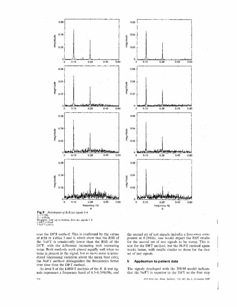
The periodograms of each of the four R-R test signals are given in Fig. 5. Fig. 5a shows the result of analysis based on the DFT, and Fig. 5b shows the result of analysis based on the NeFT.

Each periodogram shows two distinct peaks, the LF peak at 0.1Hz and the HF peak at 0.28Hz. The fre- quency resolution for the test signals is 0.001 171 Hz.

For each signal an analysis of the periodogram shows that the LF peak occurs at the 86th Fourier coefficient (0.1 OOSHz), located within wavelet level 7 (coefficients 64-127). The HF peak occurs at the 240th Fourier coefficient (0.2812Hz), located within level 8 (coefficients 1 2 8-2 5 6).

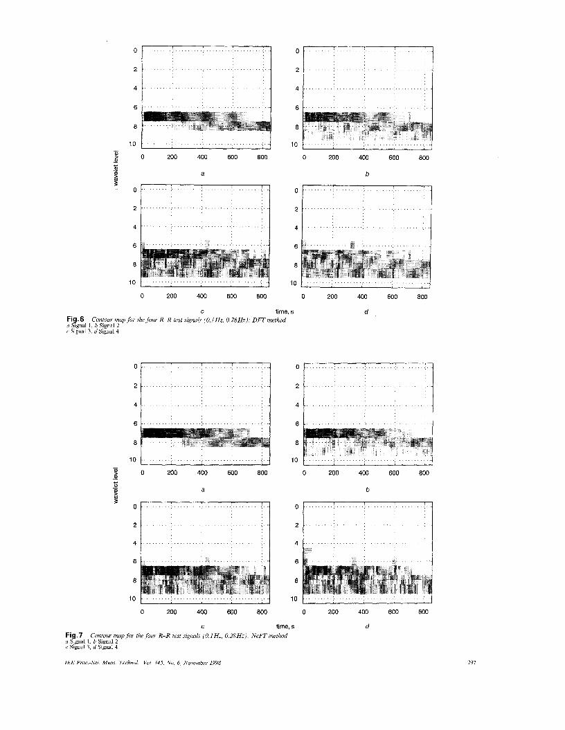
The time-frequency maps of the four R-R test sig- nals using the DFT method are shown in Fig. 6, and similar maps using the NeFT are shown in Fig. 7.

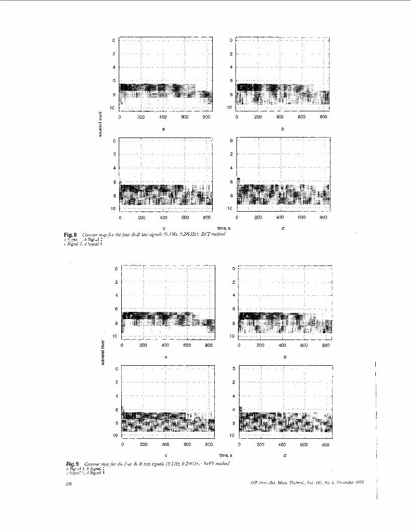
Because the HF peak of the R-R test signal (0.28Hz) falls close to the boundary between wavelet levels 8 and 9, a second set of four test signals was generated using the IPFM model with an input signal with frequencies 0.1Hz and 0.299Hz for comparison (all other parame- ters being equal to the first set of test signals).

The Fourier coefficient representing the LF compo- nent at 0.1 Hz is again in wavelet level 7, while the HF component at 0.299Hz falls between the 255th and 256th Fourier coefficient (0.2988Hz and 0.3000Hz, respectively), which means that the HF component of the signal falls between levels 8 and 9. An analysis of the Fourier coefficients reveals that the HF component is represented predominantly by the 255th coefficient for all four test signals. The results of the analysis are shown in Figs. 8 and 9.

To compare the two methods quantitatively, the wavelet maps were used to obtain individual signals for wavelet levels 7 and 8. Fig. 10 is a typical plot which shows wavelet levels 7 and 8 for test signals 1 and 2 from the first set of test signals (fl = O.lHz, fi =

0.28Hz), calculated using the NeFT method. The aver- age residual sum of squares (RSS) for these two wave- let levels was calculated for 100 randomly generated

IEE Proc -Sei Meas Technol, Vol 145, No 6, November 1998

400 600 800

time, s

realisations of test signals 2, 3 and 4, using test signal 1 as the benchmark, employing both DFT and NEFT methods. Table 3 contains the corresponding average RSS values and Table 4 shows the average RSS values calculated for 100 realisations of the second set of test signals VI = O.lHz,fi = 0.299Hz).

Table 3: Residual sum of squares (x of test signals

for the first set

Signal fq = 0.1 HZ f2 = 0.28HZ

DFT NeFT DFT NeFT

2 (S= 25) 1.226 0.852 1.572 0.774

3 (S= 50) 4.904 3.141 9.267 4.095

4 ( S = 100) 27.42 14.72 97.42 32.85

Table 4: Residual sum of squares (x IO”) for the second set of test signals

Signal fl = 0.1 HZ f2 = 0.299Hz

DFT NeFT DFT NeFT

2 (S= 25) 1.287 0.895 1.282 0.628

3 (S= 50) 4.744 3.057 7.387 3.247

4 (S= 100) 28.65 14.93 115.0 30.04

4

The periodogram plots of Fig. 5 show that the DFT and NeFT methods work equally well at determining the frequency coefficients of the test signals when no noise is present. As the test signal noise increases, the NeFT provides better analysis with less noise in the periodogram. This is to be expected since the variation about the mean beat rate of the test signals increases with noise and this affects the accuracy of the cubic spline approximation used by the DFT method.

Analysis using the DHWT shows a similar difference in the DFT and NeFT methods. When considering both sets of four R-R test signals there is a definite improvement in the quality of analysis using the NeFT

Discussion of test signal results

295

0 0.10 0.28 0.45 0.60

0.06 t

0 0.10 0.28 0.45 0.60

0.06 ~1 ,,, 0.04 U

c C U)

E" 0.02

0 0 0.10 0.28 0.45 0.60

0.06}

a, 0 0 4 -a r m

E 0.02

0 0 0.10 0.28 0.45 0.60

frequency, Hz a

Fig.5 f, = 0 1Hz.

Periodogram of R-R test signals 1-4

fi = 0 28Hz Diagrams, from top to bottom, show test signals 1 4 a DFT method b NeFT method

over the DFT method. This is confirmed by the values o f RSS in Tables 3 and 4, which show that the RSS of the NeFT is consistently lower than the RSS of the DFT, with the difference increasing with increasing noise. Both methods work almost equally well when no noise is present in the signal, but as more noise is intro- duced (increasing variation about the mean beat rate), the NeFT method distinguishes the frequencies better over time than the DFT method.

As level 9 of the DHWT analysis of the R-R test sig- nals represents a frequency band of 0.3-0.5988Hz, and

296

0 06

0.04 -3 r

0.02

0 0.28 0.45 0.60 0 0.10

0.06

0 0.10 0.28 0.45 0.60

0.06 1 4

0 0.10 0.28 0.45 0.60

0.06 1 a, 0.04 -2

E 0.02

c .- C In

0 0 0.10 0.28 0.45 0.60

frequency, Hz b

the second set of test signals includes a frequency com- ponent at 0.299Hq one would expect the RSS results for the second set of test signals to be worse. This is true for the DFT method, but the NeFT method again works better, with results similar to those for the first set of test signals.

5 Application to patient data

The signals developed with the IPFM model indicate that the NeFT is superior to the DFT as the first step

IEE Proc -Sei Meus Technol, Val 145, No 6, November 1998

'1 . . . . . . . . . . . . . . . . . . . . . . . . . . . . . . . . . . . . . .

. . . . . . . . . . . . . . . . . . . . . . . . . . . . . . . . . . . . . . .

2 O I

2

4

0

2

4

6

8

10 - 0) - 2i c - a,

0 $

2

4

. . . . . . . . . . . . . . . . . . . . . . . . . . . . . . . . . . . . . . . . . . . . . . .

. . . . . . . . . . . . . . . . . . . . . . . . . . . . . . . . . . . . . . . . . :. ..

. . . . . . . . :. . . . . . . . . .:_ . . . . . . . . . . . . . . . . . . . .:. .j

8

. . . . . . . . . . . . . . . . . . . . . . . . . . . . . . . . . . . . . . . .

0 200 400 600 800 0 200 400 600 800

b a

0 J;-1 . . . . . . . . . . . . . . . . . . . . . . . . . . . . . . . . . .

2 . . . . . . . . . . . . . . . . . . . . . . . . . . . . . . . .

4 . . . . . . . . . . . . . . . . . . . . . . . . . . . . . . . . . . . . .

10 . . . . . . . . . . . . . . . . . . . . . . . . . . . . . . . . . . . . . . . . . . . .

0 200 400 600 800 200 400 600 800 0

C time. s d Fig.6 a Signal 1, b Signal 2 c Signal 3, d Signal 4

Contour map for the jour R-R test signals (O.IHz, 0.28Hz): DFTmethod

2 Or------

4 ' 1 1 : . . . . . . . . : . . . . . . . . .:_ . . . . . . . . . . . . . . . . . . . .:. .

6 . . . . . . . . . . . . . . . . . . . . . . . . . . . . .I. . . . . . . . .

8

10 . . . . . . . . . ) . . . . . . . . . . . . . . . . . . . . . . . . . . . . . . . ' . .

0 200 400 600 800 0 200 400 600 800

b a

0 . . . . . . . ) . . . . . . . . . . . . . . . . . . . . 1 . . 1 ;

a

in . . . . . . . . . . . . . . . . . . . . : . _ . . . . . . . . :. . . . . . . . . .:. . .- I

0 200 400 600 800 0 200 400 600 800

C time, s d Fig.7 a Signal I, b Signal 2 c Signal 3, d Signal 4

Contour map for the four R-R test signals (O.IHz, 0.28Hz): NeFTmethod

IEE Pvoc.-Sei. Meas. Technol., Vol. 145, No. 6, November 1998 291

0

2

4

6

8

10

0

2

4

6

8

10

. . . . . . . . . . . . . . . . . . . . . . . . . . . . . . . . . . .

. . . . . . . . . . . . . . . . . . . . . . . . . . . . . . . . . . .

. . . . . . . . . . . . . . . . . . . . . . . . . . . . . . . . . . . . . . . .

. . . . . . . . . . . . . . . . . . . . . . . . . . . . . . . . . . . . . . . ;...I

2

4

0 200 400 600 800

. . . . . . . . . . . . . . . . . . .:. . . . . . . . . .:. . . . . . . . . .:. ..

- . . . . . . . . . . . . . . . . . . . . . . . . . . . . .:. . . . . . . . . .:. ..

a

. . . . . . . . . . . . . . . . . . . . . . . . . . . . . . . . . . . . . . .

. . . . . . . . . . . . . . . . . . . . . . . . . . . . . . . . . . . . . :...I

0 200 400 600 800

0

2

4

6

8

10

0

2

4

6

8

10

C time, s Fig.8 a Signal 1, b Signal 2 c Signal 3, d Signal 4

Contour map for the four R-R test signals (O.lHz, 0.299Hz): DFTmethod

0 . . . . . . . . . . . . .

2 . . . . . . . . . . . . . .

4 . . . . . . . . . . . . .

6 . . . . . . . . . . . . . . . .

<: : . . . . . . . . . . . . . . 8

- $ 0 200 400 600 800 -

c k, J

lo I 0 200 400 600 800

i 1

d '..A.

, ' . ? * . . . . . . . . . . . . . . . . ' ' 1 I . .:I ,

0 200 400 600 800

b

0 200 400 600 800

d

6

0 200 400 600 800

b

6 i a

C time, s

Fig.9 a Signal 1, b Signal 2 c Signal 3, d Signal 4

Contour map for the four R-R test signals (O.lHz, 0.299Hz): NeFTmethod

0 200 400 600 800

d

298 IEE Proc.-Sei. Meas. Technol., Vol. 145, No. 6, November 1998

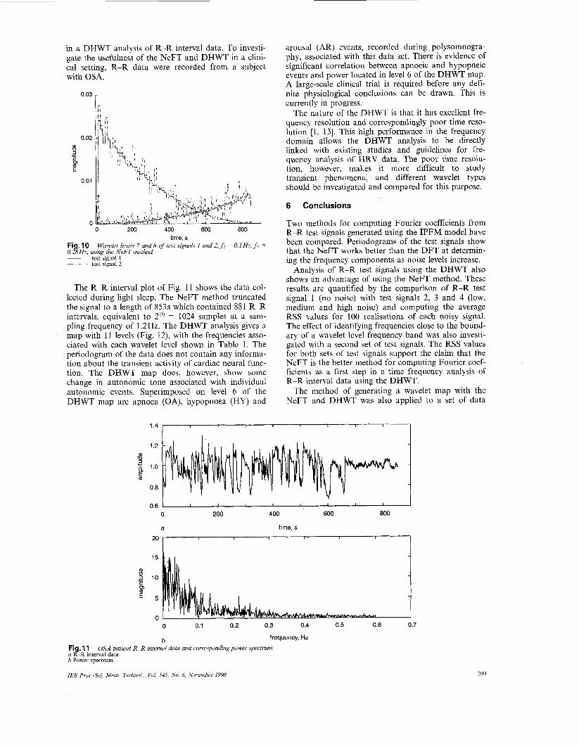
in a DHWT analysis of R-R interval data. To investi- gate the usefulness of the NeFT and DHWT in a clini- cal setting, R-R data were recorded from a subject with OSA.

0 200 400 600 800 time, s

Fig. 10 0.28Hz, using the NeFT method ~ test signal 1

test signal 2

Wavelet levels 7 and 8 of test signals 1 and 2 , f , = O.IHz,h =

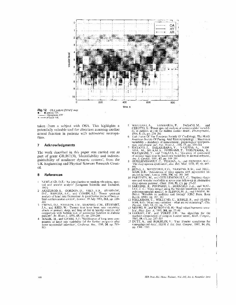
The R-R interval plot of Fig. 11 shows the data col- lected during light sleep. The NeFT method truncated the signal to a length of 853s which contained 881 R-R intervals, equivalent to 21° = 1024 samples at a sam- pling frequency of 1.2Hz. The DHWT analysis gives a map with 11 levels (Fig. 12), with the frequencies asso- ciated with each wavelet level shown in Table 1. The periodogram of the data does not contain any informa- tion about the transient activity of cardiac neural func- tion. The DHWT map does, however, show some change in autonomic tone associated with individual autonomic events. Superimposed on level 6 of the DHWT map are apnoea (OA), hypopnoea (HY) and

arousal (AR) events, recorded during polysomnogra- phy, associated with this data set. There is evidence of significant correlation between apnoeic and hypopneic events and power located in level 6 of the DHWT map. A large-scale clinical trial is required before any defi- nite physiological conclusions can be drawn. This is currently in progress.

The nature of the DHWT is that it has excellent fre- quency resolution and correspondingly poor time reso- lution [l, 131. This high performance in the frequency domain allows the DHWT analysis to be directly linked with existing studies and guidelines for fre- quency analysis of HRV data. The poor time resolu- tion, however, makes it more difficult to study transient phenomena, and different wavelet types should be investigated and compared for this purpose.

6 Conclusions

Two methods for computing Fourier coefficients from R-R test signals generated using the IPFM model have been compared. Periodograms of the test signals show that the NeFT works better than the DFT at determin- ing the frequency components as noise levels increase.

Analysis of R-R test signals using the DHWT also shows an advantage of using the NeFT method. These results are quantified by the comparison of R-R test signal 1 (no noise) with test signals 2, 3 and 4 (low, medium and high noise) and computing the average RSS values for 100 realisations of each noisy signal. The effect of identifying frequencies close to the bound- ary of a wavelet level frequency band was also investi- gated with a second set of test signals. The RSS values for both sets of test signals support the claim that the NeFT is the better method for computing Fourier coef- ficients as a first step in a time-frequency analysis of R-R interval data using the DHWT.

The method of generating a wavelet map with the NeFT and DHWT was also applied to a set of data

1.2 ar 3

1.0

0.8

0 0.1 0.2 0.3 0.4 0.5 0.6 0.7

frequency, Hz b Fig. 1 1 a R-R interval data b Power spectrum

IEE Proc.-Sei. Meas. Technol., Vol. 145, No. 6, November 1998

OSA patient R-R interval data and corresponding power spectrum

299

0

1

2

3

4

5

6

7

8

9

I 1 t I I I I I ........................................................... 1 . . . . . . . . ._.. . . . . .

. . . . . . . . . . . . . . . . . . . . . . . . . . . . . . . . . . . . . . . . . . . . . . . . . . . . . . . . . . . . . # ~~~

: -

10

0 200

Fig.12 OSApatlent DHWTmap 0-0 apnoea OA t-+ hypopnoea HY x-x arousal AR

taken from a subject with OSA. This highlights a potentially valuable tool for clinicians assessing cardiac neural function in patients with autonomic neuropa- thies.

7 Acknowledgments

The work described in this paper was carried out as part of grant GRiJ67 130, ‘Identifiability and indistin- guishability of nonlinear dynamic systems’, from the UK Engineering and Physical Sciences Research Coun- cil.

8 References

1 NEWLAND, D.E.: ‘An introduction to random vibrations, spec- tral and wavelet analysis’ (Longman Scientific and Technical, 1993)

2 AKSELROD, S., GORDON, D., UBEL, F.A., SHANNON, D.C., BARGER, A.C., and COHEN, R.J.: ‘Power spectrum analysis of heart rate fluctuation: A quantitative probe of beat-to- beat cardiovascular control’, Science, 10 July 1981, 213, pp. 220- 222 EWING, D.J., NEILSON, J.M., SHAPIRO, C.M., STEWART, J.A., and REID, W.: ‘Twenty four hour heart rate variability: effects of posture, sleep, and time of day in healthy controls and comparison with bedside tests of autonomic function in diabetic patients’, Br. Heart J., 1991, 65, (5), pp. 239-244

4 MALIK, M., and CAhllM, A.J.: ‘Significance of long term com- ponents of heart rate variability for the further prognosis after acute myocardial infarction’, Cardiovas. Res., 1990, 24, pp. 793- 803

3

400 600 800

time. s

5 MALLIANI, A., LOMBARDI, F., PAGANI, M., and CERUTTI, S.: ‘Power spectral analysis of cardiovascular variabil- ity in patients at risk for sudden cardiac death’, Electrophysiol., 1994, 5, (3), pp. 274286

6 Task Force Of The European Society Of Cardiology, The North American Society Of Pacing, And Electrophysiology, : ‘Heart rate variability - standards of measurement, physiological interpreta- tion, and clinical use’, Eur. Heart J., 1996, 17, pp. 354-381

ADA, M., MUKAI, S., FUJINAMI, T., YOKOYAMA, K., WATANABE, Y., and TAKATA, K.: ‘Accuracy of assessment of cardiac vagal tone by heart rate variability in normal subjects’, Am. J. Cardiol., 1991, 67, pp. 199-204 GUILLEMINAULT, C., TILKIAN, A., and DEMENT, W.C.: The sleep apnoea syndromes’, Ann. Rev. Med., 1976,27, pp. 465- 484

9 HUNG, J., WHITFORD, E.G., PARSONS,,R.W., and ,HILL- MAN, D.R.: ‘Association of sleep apnoea with myocardial inf- arction in men’, Lancet, 1990, 336, pp. 261-264

10 PARTINEN, M., and GUILLEMINAULT, C.: ‘Daytime sleepi- ness and vascular morbidity at seven year follow-up in obstructive sleep apnoea patients’, Chest, 1990, 91, (l), pp. 27-32

11 SARTENE, R., POUPARD, L., BERNARD, J.-L., and WAL- LET, J.-C.: ‘Sleep images using the wavelet transform to process polysomnographic signals’, in ALDROUBI, A., and UNSER, M. (Eds.): ‘Wavelets in medicine and biology’ (CRC Press, Boca Raton, 1996), pp. 355-382

12 NIKLASSON. U.. WIKLUND. U,. BJERLE. P.. and OLOFS-

7 HAYANO, J., SAKAKIBARA, Y., YAMADA, A., YAM-

8

13

14

, I

iriation - what are we measuring?’, Clin.

TANI, H.: ‘Real-valued harmonic wave-

J.W.: ‘An algorithm for the machine computation of complex Fourier series’, Math. Compuf.,

71-79

. 53-60

1965, 19. (1). UV. 297-301 15 DUTT, A:,’yLd ROKHLIN, V.: ‘Fast Fourier transforms for

nonequispaced data’, SIAM J. Sci. Stat. Comput., 1993, 14, (6), pp. 1368-1393

300 IEE Proc.-Sci. Meas. Technol., Vol. 145, No. 6, November 1998