Contents lists available at ScienceDirect

Computers and Electrical Engineering

journal homepage: www.elsevier.com/locate/compeleceng

Comparison of lossless compression schemes for high rate electricalgrid time series for smart grid monitoring and analysis☆

Richard Jumar⁎, Heiko Maaß, Veit HagenmeyerKarlsruhe Institute of Technology - Institute for Automation and Applied Informatics, Kaiserstraße 12, Karlsruhe 76131, Germany

A R T I C L E I N F O

Keywords:Time seriesLossless compressionSignal representationPower grid monitoringSmart gridPower quality

A B S T R A C T

The smart power grid of the future will utilize waveform level monitoring with sampling rates inthe kilohertz range for detailed grid status assessment. To this end, we address the challenge ofhandling large raw data amount with its quasi-periodical characteristic via lossless compression.We compare different freely available algorithms and implementations with regard to com-pression ratio, computation time and working principle to find the most suitable compressionstrategy for this type of data. Algorithms from the audio domain (ALAC, ALS, APE, FLAC &TrueAudio) and general archiving schemes (LZMA, Delfate, PPMd, BZip2 & Gzip) are testedagainst each other. We assemble a dataset from openly available sources (UK-DALE, MIT-REDD,EDR) and establish dataset independent comparison criteria. This combination is a first detailedopen benchmark to support the development of tailored lossless compression schemes and adecision support for researchers facing data intensive smart grid measurements.

1. Introduction

The emerging deployment of decentralized power injection devices and smart appliances increases the number of switch-modepower supplies and the occurrence of incentive based switching actions on the prosumer end of the power line. Therefore theoperational stability of future smart grids will likely depend on monitoring this behavior with high time resolution to correctly assessthe power grid status [1].

While many power grid measurement applications rely on data sampled at frequencies in the kilohertz range, the level of ag-gregation and the report rate differ. Phasor Measurement Units (PMUs) usually report on basis of 10th of milliseconds1 while smartmeters use rates between seconds for momentary data and one day for accumulated consumption [2]. This aggregation relaxes therequirements for communication channels and storage space tremendously. For power quality (PQ) monitoring and load dis-aggregation additional information is needed [3,4]. So far widely used aggregated features like harmonics can only partly providethis information so that new features are developed [5,6]. Due to ongoing changes in grid operation strategies and demand sidemanagement and due to the increase in decentralized generation, so far unknown combinations of disturbances can appear [7]. Thiscan result in unreliability of feature-based approaches since information is lost especially during interesting, usually short events.

Commercially available PQ-measurement devices use a threshold-based approach with user-configurable thresholds serving asevent indicators [8,9]. After an event is triggered, raw data are recorded for a short period of time with sampling rates from 10 kHz to10MHz. For a future smart grid, however, thresholds are hardly definable beforehand [1]. Furthermore, the evaluation of raw data

https://doi.org/10.1016/j.compeleceng.2018.07.008Received 6 November 2017; Received in revised form 17 July 2018; Accepted 18 July 2018

☆ Reviews processed and recommended for publication to the Editor-in-Chief by Associate Editor Dr. A. Isazadeh.⁎ Corresponding author.E-mail address: richard.jumar@kit.edu (R. Jumar).

1 Requirements for PMUs are defined in IEEE Std C37.118.1-2011.

Computers and Electrical Engineering 71 (2018) 465–476

0045-7906/ © 2018 The Authors. Published by Elsevier Ltd. This is an open access article under the CC BY license (http://creativecommons.org/licenses/BY/4.0/).

T

from synchronized measurements at different locations may give valuable, additional insights, even and especially in case that not alldistributed devices could classify the event at the same time and thus did not capture the event in high resolution. Data-drivenresearch aiming for developing better event classification and smart grid analysis techniques would therefore profit from a con-tinuous storage of raw data. Here, lossless data compression eases the challenge of storing and transmitting large data amount.

Usually, the data stream from a raw data recorder comprises three channels with voltage measurements (from the three phases)and four current channels (three for the phase currents and one for the neutral conductor). In a three phase power system voltagecurves are nominally sinusoidal and phase shifted by 120°. This results in a strong correlation between the channels. This is also holdsfor current channels and utilizing this correlation provides room for significant data reduction. In a real world scenario, however, thewaveforms are individually distorted, reducing the degree of correlation. Especially the current channels are expected to be lesscorrelated as the individual phase-loads cause different phase-shifts and distortions. With respect to the distortion must be noted, thatwave forms only change when the device connection status or power demand changes. These processes are usually slow compared tothe timespan of one period. In a scenario where few loads are connected to the monitored grid, the waveform changes occur rarely.When a large number of loads is connected to the monitored section of the grid, changes occur often but are usually small inamplitude due to the summation of load currents. Both aspects suggest that there is potential for waveform compression. For specificpurposes such as audio and video highly efficient lossless compression algorithms exist [10], however, none could be found that isespecially tailored to exploit the strong periodic behavior and multichannel characteristic of the encountered electrical signals in thesense of a stream compression.

The use of event data compression methods i.e. the compression of small sections of waveform data from a single channel ishowever reported in literature: Although focusing on lossy techniques, [11] provides an overview with technical explanations also forlossless schemes together with experimental compression rate (CR) values. The compression of PQ-event data is the focused appli-cation, handling quasi static data is not addressed. Using a delta modulation approach and subsequent Huffman-coding, CRs of 2 areyielded when averaging over different PQ-event types [12]. Pure Huffman-coding alone results in CRs with a maximal value of 1.1. Acomparison of Huffman, arithmetic and LZ-coding for different PQ-events (flicker, harmonics, impulse, sag and swell) is given in[13]. CRs are between 1.7 and 1.9 for LZ, 1.18 and 2.78 for arithmetic, 1.23 to 2.81 for Huffman-coding respectively. Thereby thecited authors use own implementations. A compression of long term raw data is not performed and information on the statisticalevaluation is not available. Gerek and Ece present tests with the ZIP-software and achieve CRs of 5 on average on grid raw data [14].The authors verified the lossless operation of the codec but halved the vertical resolution of input data to 8 bit before the compressionfor compatibility with their own implementation. They also present test results on the compression techniques Free Lossless AudioCodec (FLAC) and True Audio (TTA) yielding CRs between 4 and 5 on average when using their own set of voltage measurements,taken in a laboratory environment with a mixture of RL load banks, induction motors and frequency converters. Sample-size andfurther statistical aspects are not reported. The effect of the acquisition rate on compression ratio is studied in [15]. The authors alsocompare the integer representation AXDR2 with a lightweight derivative of the Lempel-Ziv-Markov chain Algorithm (LZMA) calledLZMH and a differential coding approach called DEGA [16] on waveform data. Both methods were originally developed to compressaggregated data from smart meters with low computational effort. The CR comparison for raw data, however, includes a formatconversion factor. Comma-separated-value files (probably ANSI) are compared with the binary output of the algorithms. By doing so,the conversion from a 4 to 7 digit fixed point (” ± 327.68”) ASCII representation to an unsigned 16-bit integer representation isincluded in the measurements. This alone accounts for a CR result of 2 to 3.5 which is not caused by actually compressing thewaveform. They therefore report CRs as high as 9 on average for a one-week set of current waveforms from UK-DALE. As qualitativeobservations an increase in CR with increasing sample frequency fs roughly proportional to log(fs) from 1 kHz upwards and thesuperiority of differential coding combined with an entropy stage over LZMH are reported.

To the best of our knowledge, literature treats existing lossless compression codecs in the application for power gird waveformdata only as a side-issue. No reproducible description of an experiment with sound statistical evaluation is available. The referencedstudies use very specific event data for proving the suitability of algorithmic modifications for their special cases only. Additionally,data sources are neither referenced nor provided in most cases. Together with the observed scatter of the reported compression ratiosfor established methods, we conclude, that there is no reference for researchers to judge on the suitability of compression methods forgrid waveform data - be it existing techniques or new developments.

Therefore, the aim of the present contribution is to explicitly focus on a comparison by testing different open out-of-the-boxlossless compression algorithms and implementations for high-sampling-rate data from the power grid. Using codecs with differentcompression principles, we intend to gain insights for future developments that rely on raw time series evaluation. The test datatogether with the established comparison criteria serve as a first detailed open benchmark which supports the development oftailored lossless compression schemes. Furthermore it serves as a decision support for researchers facing data intensive smart gridmeasurements.

The remainder of the article is structured as follows. Our test data sources are presented in Section 2, while Section 3 lists thecodecs we use and describes their fundamentals. Section 4 deals with the experimental set-up. Results are presented in Section 5 anddiscussed in Section 6. The article closes with conclusions in Section 7.

2 Abstract eXternal Data Representation (AXDR) is an integer encoding rule for distribution automation using line carrier systems, defined bystandard IEC61334-6:2000.

R. Jumar et al. Computers and Electrical Engineering 71 (2018) 465–476

466

2. Datasets

The UK Domestic Appliance-Level Electricity Dataset (UK-DALE) [17] includes, inter alia, raw data from current and voltagemeasurements taken at the in-feeds of three houses. The acquisition was performed with audio-inspired equipment at a sampling rateof 16 kHz and 24 bit vertical resolution. From this FLAC-compressed set we chose data from house 1 and randomly selected six filesfrom the recording period between 2014-8-08 and 2014-05-15, each containing one hour of recording.3

The Energy Disaggregation Dataset MIT-REDD [18] also provides high frequency raw data acquired at the central connectionpoints of houses. Current and voltage values are recorded at 15 kHz sampling frequency and stored in a proprietary format as four-byte floating point numbers interleaved with timestamps. From the openly available excerpt we use all 21 files containing voltagevalues and all current files from phase 2 of house 5. Each file is 266 s in length.

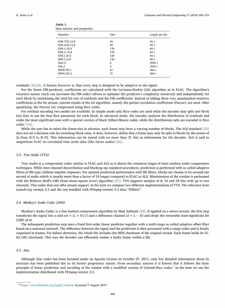
At KIT, we are performing high rate current and voltage measurements of the power supply grid using our own device, theElectrical Data Recorder (EDR) [19]. All data are transferred over the network and stored in the Large Scale Database [20] at KIT. Thedata amount for raw data storage per day is 8.4 GiB for three phase voltages and 19.35 GiB for three phase currents (plus neutral) andvoltage captures. The transmission requires a bandwidth of 0.8Mbit/s and 1.8Mbit/s, respectively [21]. The present dataset wasacquired at the following locations: The central feed of our institute building, at a power socket in our experimental hall and at asubstation transformer in the city of Karlsruhe, Germany. Sampling rates of 12.8 kS/s and 25 kS/s (four currents and three voltages, 7channels in total) are used. For the single and dual channel tests, we pick current and/or voltage of one phase. Data are stored inblocks of 60 s as 16-bit raw values and are available at [22]. Table 1 gives an overview of the data used.

2.1. Preparation of data

As input data format for our study we chose the RIFF WAV format with 16-bit signed integer representation for the followingreasons: (1) It allows the seamless testing of audio codecs; (2) It is the most basic and common format for waveform data with onlyvery little overhead and no additional redundancy; (3) It is very close to the typical output of analog-to-digital converters.

With respect to UK-DALE data we used SoX4 for the conversion and to separate the current and voltage channels (left and rightaudio channel of the file). Preprocessing the MIT REDD involved deleting the time stamps, normalizing the amplitudes for each fileand a float-to-integer conversion so that the absolute maximum gets mapped to −2 115 or − 2 ,15 respectively. EDR data only neededthe addition of the RIFF WAV-header.

3. Codecs and algorithms

In this section we give an overview on the used algorithms and implementations. We choose free software from the generalpurpose domain and the lossless audio compression domain.

3.1. FLAC

FLAC is an acronym for Free Lossless Audio Codec and it may be the first fully free audio codec [10]. The input stream is dividedinto blocks of user-defined sizes on which the further processing is performed. For multichannel signals (up to eight channels aresupported), each block contains one sub-block for each channel without interleaving. Two different signal approximation methodsare available. The fixed linear predictor fits a Lagrange polynomial up to the 4th order to the audio samples of a block. A 3-bit numberis then added to the stream for encoding the chosen order of prediction [10].

The more advanced FIR (finite impulse response) predictor also called LPC (Linear Predictive Coding) is of variable order with themaximum ≤ 32 specified by the user [23]. Coefficients are calculated using the Levinson–Durbin algorithm and added to the stream.LPC yields 5–10% smaller files than the simple predictor when used on audio data.

Residuals are then encoded using Rice codes with the encoder estimating the shape of the Laplace distribution to define theoptimal Rice parameter. To handle changing distributions, the encoder may split up a sub block into 2m partitions and determines theRice parameter and the partition size for each part. In an iterative process, the partitioning scheme (m) is selected so that the size ofthe sub-block is minimized. The format specific meta-data is stored in each frame and allows for sample accurate searching, streaming(no further data required) and error resistance. This can be complemented by user-defined meta-data models. Sampling rates from1 Hz to 1,048,570 Hz (in 1-Hz increments) are supported [23].

In the tests we compare two different implementations of FLAC: The reference from Xiph.org [23] version 1.3.2 and the onebundled with FFmpeg-version 3.3 alias ”Hilbert”.5

3.2. MPEG-4 ALS

ALS uses the following steps: Block partitioning, prediction (short and long term), joint channel coding and entropy coding of the

3 The names of the used files end on: 340892, 300677, 430750, 753990, 948996, 162008.4 SoX - Sound eXchange Homepage: http://sox.sourceforge.net Accessed 13 June 2017.5 FFmpeg-Project: http://ffmpeg.org Accessed 30 June 2017.

R. Jumar et al. Computers and Electrical Engineering 71 (2018) 465–476

467

residuals [10,24]. A feature however is, that every step is designed to be adaptive to the signal.For the linear FIR-predictor, coefficients are calculated with the Levinson-Durbin (LD) algorithm as in FLAC. The algorithm’s

recursive nature (each run increases the FIR-order) allows to optimize the predictor’s complexity iteratively and independently foreach block by minimizing the total bit rate of residuals and the FIR-coefficients. Instead of adding these very quantization-sensitivecoefficients to the bit stream, interim results of the LD algorithm, namely the partial correlation coefficients (Parcor), are used. Afterquantizing, the Parcors are compressed using Rice codes.

For residual encoding two modes are available. In simple mode only Rice codes are used while the encoder may split one blockinto four to use the best Rice parameter for each block. In advanced mode, the encoder analyses the distribution of residuals andcodes the most significant ones with a special version of block Gilbert-Moore codes, while the distributions tails are encoded in Ricecodes [10].

While the user has to select the frame-size in advance, each frame may have a varying number of blocks. The ALS standard [25]does not set a decision rule for switching block-sizes. It does, however, define that a frame may only be split in blocks by the power of2s from N/2 to N/32. This information can be stored with no more than 31 bits as information for the decoder. ALS is said tooutperform FLAC on correlated time series data (like stereo audio) [26].

3.3. True Audio (TTA)

True Audio is a compression codec similar to FLAC and ALS as it shares the canonical stages of most modern audio compressiontechniques. While inter-channel decorrelation and blocking use standard procedures, prediction is performed with so called adaptivefilters of IIR-type (infinite impulse response). For optimal prediction performance with IIR filters, blocks are chosen to be around onesecond of audio which is usually more than a factor of 10 longer compared to FLAC or ALS. Minimization of the residue is performedwith the Widrow–Hoff’s LMS (least mean square error) algorithm [27]. TTA supports samples of 8, 16 and 24 bits with up to twochannels. This codec does not offer stream support. In the tests we compare two different implementations of TTA: The reference fromtausoft.org version 2.3 and the one bundled with FFmpeg-version 3.3 alias ”Hilbert”.

3.4. Monkey’s Audio Codec (APE)

Monkey’s Audio Codec is a free lossless compression algorithm by Matt Ashland [28]. If applied on a stereo stream, the first steptransforms the signal into a mid ( = +m L R( )/2) and a difference channel ( = −d L R) and drops the restorable least-significant bit(LSB) of m.

The subsequent prediction step uses a fixed first-order linear predictor together with a multi-stage so called adaptive offset filterbased on a neuronal network. The difference between the signal and the prediction is then processed with a range coder and is finallyorganized in frames. For failure detection, the whole file includes the MD5 checksum of the original stream. Each frame holds its 31-bit CRC checksum. This way the decoder can efficiently isolate a faulty frame within a file.

3.5. Alac

Although Alac codec has been licensed under an Apache License on October 27, 2011, only few detailed information about itsstructure has been published due to its former proprietary nature. From secondary sources it is known that it follows the basicprinciple of linear prediction and encoding of the residue with a modified version of Golomb-Rice codes.6 In the tests we use theimplementation distributed with FFmpeg-version 3.3.

Table 1Data sources and properties.

Identifier Files Length per file

EDR_7CH_12.8 60 60 sEDR_2CH_12.8 60 60 sEDR_U_25.0 120 60 sEDR_U_12.8 120 60 sEDR_I_25.0 120 60 sEDR_I_12.8 120 60 sDale_U 6 3600 sDale_I 6 3600 sREDD_H5_I 21 266 sREDD_H5_U 21 266 s

6 https://en.wikipedia.org/Apple_Lossless Accessed 7 August 2017.

R. Jumar et al. Computers and Electrical Engineering 71 (2018) 465–476

468

3.6. 7zPPMd

PPMd is the 7zip implementation of Dimitri Shakarin’s PPMdH variant [10]. Prediction by Partial Matching (PPM) uses arithmeticcoding where the probabilities of symbols are determined by the context in which they appear. The principle of arithmetic coding isto assign a non-integral number of bits to a symbol in order to exactly match its information content log2(ps), where ps is therespective probability of occurrence of each symbol [10]. The PPM algorithms use Markov models of different, adaptive order forcontext modeling. PPM variants (A,B,P,X & D) mainly differ in the way zero frequency symbols – i.e. symbol combinations that havenot been seen so far – are handled. Thereby PPMd uses a technique called information inheritance [29]. Memory requirements andspeed are the same for compression and decompression. We use PPMd with a memory size of 16 MB and an 8th-order model.

3.7. BZip2

BZip2 makes use of the Burrow-Wheeler method [10]. The idea is to rearrange symbols for a more efficient subsequent com-pression. A block of input data (S) is cyclically shifted by one symbol and these rotations are temporarily sorted in a table - each rowbeing one rotation. Rows are then lexicographically sorted with an index I that points to the original. The last column of the table isthen taken as the output data together with I. This concentrates the occurrence of same symbols based on the context i.e. the previoussymbols [30].

The output is then compressed with run-length coding, move-to-front coding and Huffman coding. Depending on the data,compression can be up to one bit per byte [10]. The multi-stage-approach together with required sorting makes Bzip2 comparativelyslow but efficient. To further increase compression ratio, multiple runs can be used. We use the 7zip-implementation in ”Ultra”-modewith a block size (dictionary) of 900 k and 7 consecutive runs with the multiprocessor switch disabled.

3.8. DEFLATE, DEFLATE64 and Gzip

DEFLATE and DEFLATE64 are based on LZ77 and combine it with Huffman codes [10]. The LZ77 searches a look-ahead buffer (socalled ”fast bytes”) for matches with the latest part of the stream seen so far (the search buffer). This sliding search window has aslength of up to 32 kB with DEFLATE and 64 kB with DEFLATE64. Matches are then identified by tokens (length of the match anddistance) and these tokens are Huffman-coded and written to the output stream. In case no match is found, the symbol itself isHuffman-coded and reported. DEFLATE uses two Huffman-Tables, one for length and symbols, the other for distances. Depending onselected options a fixed code table is used or individual tables are generated. Gzip is a software package that utilizes the zlib libraryby Jean-Loup Gailly and Mark Alder, that implements the .gzip-file format and the DEFLATE algorithm [10]. All three algorithms areused in 7Zip-implementation in ”Ultra”-mode with a 128-byte look-ahead-buffer and 10 passes.

3.9. 7z and LZMA

The Lempel-Ziv-Markov-chain-Algorithm is the main technique used by the free windows software package 7-Zip, both by IgorPavlov [10]. The algorithm itself is an extension of LZ77. It is similar to DEFLATE but uses range-coding instead of Huffman-coding tocompress data near the entropy limit. Range coding is the integer variant of arithmetic coding. LZMA uses only integer operations.

Like DEFLATE, LZMA also outputs length and distance of a match between preview and search buffer, but keeps a four entryhistory of the distances. This way a 2-bit number is enough output instead of the potentially very long distance if the current distanceis in the history [10].

As a test for the subsequent evaluation we ran the 7z-package (referenced as 7zip) and LZMA separately, each with ”Ultra”-modesettings, which should yield same results. The settings are in detail: 64 fast bytes, 64 MB dictionary size, 48 passes, binary-tree-matching, 3 literal context bits and 2 low-bits at current position.

4. Experimental set-up

Each codec is applied to all test datasets one after the other (single threaded). The codecs are run on a standard Windows 8.1 x64PC (Intel(R) Core(TM) i5-2500 CPU @ 3.30 GHz 3.29 GHz). File reading and storage is performed on a SSD drive, which has asequential read benchmark of 282.376MB/s and a sequential write benchmark of 239.351MB/s (values determined by Chrystal Discmark 5.2.1). We use the out-of-the-box command line implementations of ffmpeg (version 3.3 Hilbert),7 7zip (version 17.00),8 FLAC(version 1.3.2) [23], TTA (version 2.3) [27], APE (version 4.25) [28] and MPEG4 ALS (version 2.3) [24]. The general purposecompression methods are run with the highest possible CR setting. The audio codecs were run using default settings. We use thecommands from Table 2 for compression.

The computation times of a single conversion (CT) and reconversion (DCT) are calculated by the difference of the computersystem time before and after the command line tool execution. The codec is run for each input test file of each source for compressionand decompression. We compared the decompressed files with the input on byte-level to verify the lossless operation. Sources are as

7 FFmpeg-Project: http://ffmpeg.org Accessed 30 June 2017.8 7-Zip.de: http://www.7-zip.de Accessed 30 June 2017.

R. Jumar et al. Computers and Electrical Engineering 71 (2018) 465–476

469

shown in Table 1, where _U denotes voltage and _I denotes current waveforms. The compression ratios (CR) are calculated as quotientof the size of the input files and the size of the output files. The 36-Byte RIFF WAV header (RIFF and fmt part) is included in bothmeasures and causes overhead error. However, its size is very small compared to the data section that is at least 1.46 MiB in ourexperiments. Mean source performance values are derived from the average of the single file measurements for each source. Overallperformance results are the averaged codec values over all sources. We keep maximum and minimum times and ratios from eachsingle file conversion in order to depict the range of scatter of the measurements by the error indicators in the figures. For somecompression runs the execution times were rather small i.e. in the range of some hundreds of a second, which is close to systemperformance delays. In these cases, the standard deviation was high, which may not correlate with the real causes. Thus, we decidednot to show error indication with the calculated standard deviations.

Runtime variations between datasets (e.g. due to different file sizes) result in unbalanced averaged over all runtimes (long timeshave larger impact than shorter ones). Therefore we decided to normalize CT and DCT by the mean CT and DCT of the DEFLATE codefor each dataset. We picked the DEFLATE results for their consistently small standard deviation within the datasets. As a file sizeindependent general execution speed measurement we included the throughput in MiB/s. For better over-all visualization we in-troduce the following ranking scheme: For the mean values of relative CT, relative DCT and CR we perform a min-max normalizationand calculate the equally weighted average from this three parameters as performance indicator. CT and DCT values are inverted( − x1 ) so that shorter times result in higher ranking.

5. Results

Some of the conversions failed systematically, out of reasons still not clarifyable to the best of our knowledge. Although weconverted all signals to RIFF WAVE format, the REDD dataset was not able to be compressed successfully with MP4 ALS and TTA 2.3.Additionally, FLAC 1.3.2, TTA 2.3 and APE did not succeed with the 7 channel dataset. Thus, we just skipped these evaluations.

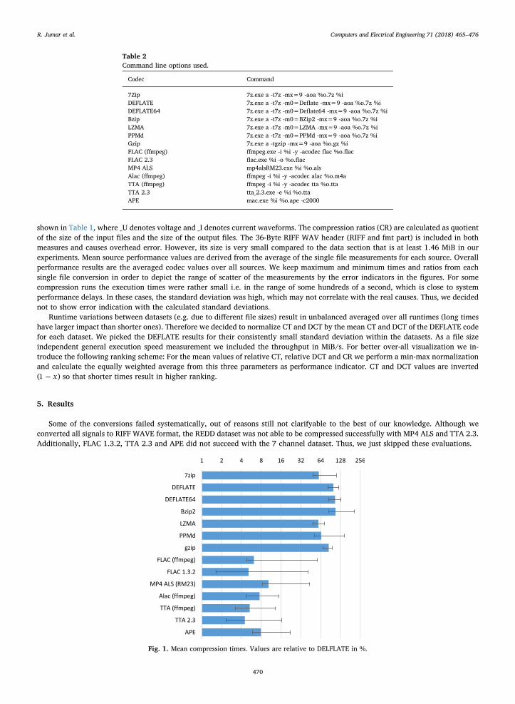
Table 2Command line options used.

Codec Command

7Zip 7z.exe a -t7z -mx=9 -aoa %o.7z %iDEFLATE 7z.exe a -t7z -m0=Deflate -mx=9 -aoa %o.7z %iDEFLATE64 7z.exe a -t7z -m0=Deflate64 -mx=9 -aoa %o.7z %iBzip 7z.exe a -t7z -m0=BZip2 -mx=9 -aoa %o.7z %iLZMA 7z.exe a -t7z -m0=LZMA -mx=9 -aoa %o.7z %iPPMd 7z.exe a -t7z -m0=PPMd -mx=9 -aoa %o.7z %iGzip 7z.exe a -tgzip -mx=9 -aoa %o.gz %iFLAC (ffmpeg) ffmpeg.exe -i %i -y -acodec flac %o.flacFLAC 2.3 flac.exe %i -o %o.flacMP4 ALS mp4alsRM23.exe %i %o.alsAlac (ffmpeg) ffmpeg -i %i -y -acodec alac %o.m4aTTA (ffmpeg) ffmpeg -i %i -y -acodec tta %o.ttaTTA 2.3 tta_2.3.exe -e %i %o.ttaAPE mac.exe %i %o.ape -c2000

Fig. 1. Mean compression times. Values are relative to DELFLATE in %.

R. Jumar et al. Computers and Electrical Engineering 71 (2018) 465–476

470

In Fig. 1 the relative compression time results of all used codecs is shown as a bar chart, scaled logarithmically in percent. The barlength corresponds to the mean value of each codec related to the DEFLATE-methods averages and the error indicators show theminimum and the maximum single run relative results.

In Fig. 1 can be seen, that audio codecs clearly outperform the non-audio codecs regarding mean compression times (CT). Therebythe audio-codecs TTA 2.3 and FLAC 1.3.2 showed best compression times. However, the variability between the compression runswas very high. The standard deviation of the compression ratios of one dataset per compression method was generally below 15 % ofthe mean values, in most cases below 5 %. However, some conversion runs of the same input source showed standard deviations up to85 % (especially, both FLAC codecs and in some cases MP4 ALS). In addition, differences between the implementation of the FLACand the TTA codecs are visible. When applying the respective ffmpeg instance, the conversion took more time. Considering non-audiocodecs only, the LZMA method was found to perform fastest on average and it was able to compress as the quickest (especially onEDR_I_12.8 [kHz] current values).

In Fig. 2, the mean compression ratios of all used codecs are shown as a bar chart on a linear scale. The error indicators depict themaximum and minimum single run results. All compression ratios of all codecs are found between 1.06 and 4.44. A slight differencetowards higher ratios can be observed with audio-codecs. The highest ratio of a single run coding was conducted with the MP4 ALScompressing EDR_I_25 [kHz] current values. Among the non-audio codecs, PPMd showed the best compression ratio on average.Again, the range between minimum and maximum results was large, but the standard deviation of the compression ratios of onedataset type per compression method was generally below 12 % of the mean values, in most cases below 4 %. Hence, the variationsresult from differences between the dataset types.

While the average CRs of the audio codecs differ only moderately, the general purpose schemes show larger differences andclustering. PPMd, LZMA, 7Zip and Bzip2 all yield better results than both DEFLATE methods and gzip. For the three latter ones alsothe variation is significantly smaller compared to PPMd, LZMA, 7Zip and Bzip2.

In Fig. 3 the mean decompression time results are shown, each again related to the DEFLATE mean decompression time of therespective dataset type. Similar to the compression time results, decompression times are considerably shorter with audio codecs thanusing non-audio codecs. Thereby FLAC and TTA perform best. The standard deviation of the decompression ratios of one dataset percompression method was generally below 10 % of the mean values, in most cases below 5 %. As like the compression time results, theFLAC-methods showed higher standard deviations for decompression. Interestingly, the PPMd codec is the worst codec regardingdecompression time.

Fig. 4 shows a comparison between current and voltage signal compression. Mean compression ratios (CR) mean, relativecompression times (CT) and decompression times are illustrated for each audio compression codec. The compression ratios of currentwaveforms are always higher than those of voltage waveforms. However, voltage time series compression is always faster thanpacking current time series. Almost the same applies to decompression duration, except TTA (ffmpeg).

In order to look at dataset-dependencies, we do a split analysis of CR, CT and DCT for each codec on all of the datasets. For reasonsof clarity we do not plot min-max bars in the following figures. The mean compression bit rate results are compared in Fig. 5. In thischart, major differences are visible between the datasets and between the codecs, applied on the same time series source. Thecompression bit rate is best for FLAC 1.3.2 to almost all datasets. TTA and the FLAC (ffmpeg) implementations are among the topperformers. MP4 ALS, Alac (ffmpeg) and APE are performing worse.

In Fig. 6, the mean compression ratios of the audio-codecs are compared for each input dataset type. The codecs are roughlysorted by best values. Apparently, the differences between the codecs applied to one dataset type is rather small compared to thedifferences between the datasets. The compression ratio strongly depends on the sampling rate of the input source. For a clearexample, the EDR_I_25.0 [kHz] dataset was compressed at almost double the size reduction of EDR_I_12.8 [kHz]. Multichannel data

Fig. 2. Mean compression ratios.

R. Jumar et al. Computers and Electrical Engineering 71 (2018) 465–476

471

from EDR are compressed at rates between those of the single channel runs with current and voltage data at the same sampling rate.In Fig. 7 the compression ratios of the non-audio methods are compared by dataset type. Using non-audio-codecs, the reached

maximum compression ratios are slightly lower than using audio-compression techniques. PPMd, Bzip2 and 7zip/LZMA form awinning-cluster as they all reach similar and higher reduction rates than DEFLATE/64 and gzip on every dataset. The differenceamong the winners is always smaller than the distance to DEFLATE/64. Also, towards the lower performance end the stacking isconstant: gzip (always loosing), DEFLATE and DEFLATE64. As with the audio codecs, ratios are strongly dataset-dependent but thedifference between ratios of the non-audio-codecs is also greater.

Fig. 3. Mean decompression times. Values are relative to DELFLATE in %.

Fig. 4. Comparing audio codecs on voltage vs. current time series. CT and DCT are relative to DEFLATE [%].

Fig. 5. Mean compression bit rates [MiB/s] of audio codecs.

R. Jumar et al. Computers and Electrical Engineering 71 (2018) 465–476

472

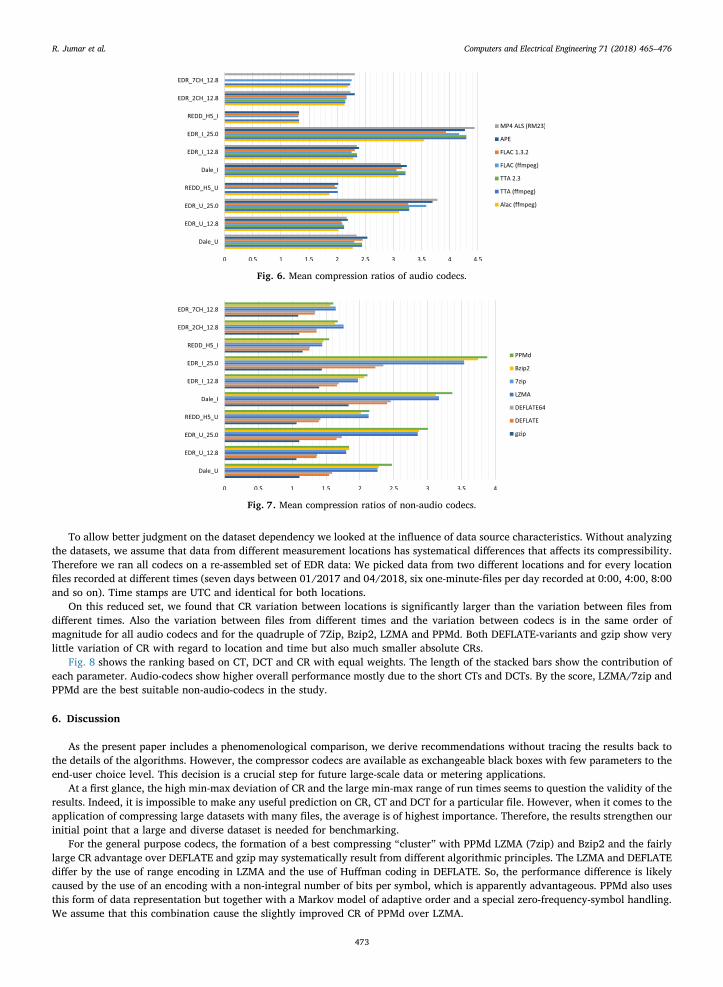
To allow better judgment on the dataset dependency we looked at the influence of data source characteristics. Without analyzingthe datasets, we assume that data from different measurement locations has systematical differences that affects its compressibility.Therefore we ran all codecs on a re-assembled set of EDR data: We picked data from two different locations and for every locationfiles recorded at different times (seven days between 01/2017 and 04/2018, six one-minute-files per day recorded at 0:00, 4:00, 8:00and so on). Time stamps are UTC and identical for both locations.

On this reduced set, we found that CR variation between locations is significantly larger than the variation between files fromdifferent times. Also the variation between files from different times and the variation between codecs is in the same order ofmagnitude for all audio codecs and for the quadruple of 7Zip, Bzip2, LZMA and PPMd. Both DEFLATE-variants and gzip show verylittle variation of CR with regard to location and time but also much smaller absolute CRs.

Fig. 8 shows the ranking based on CT, DCT and CR with equal weights. The length of the stacked bars show the contribution ofeach parameter. Audio-codecs show higher overall performance mostly due to the short CTs and DCTs. By the score, LZMA/7zip andPPMd are the best suitable non-audio-codecs in the study.

6. Discussion

As the present paper includes a phenomenological comparison, we derive recommendations without tracing the results back tothe details of the algorithms. However, the compressor codecs are available as exchangeable black boxes with few parameters to theend-user choice level. This decision is a crucial step for future large-scale data or metering applications.

At a first glance, the high min-max deviation of CR and the large min-max range of run times seems to question the validity of theresults. Indeed, it is impossible to make any useful prediction on CR, CT and DCT for a particular file. However, when it comes to theapplication of compressing large datasets with many files, the average is of highest importance. Therefore, the results strengthen ourinitial point that a large and diverse dataset is needed for benchmarking.

For the general purpose codecs, the formation of a best compressing “cluster” with PPMd LZMA (7zip) and Bzip2 and the fairlylarge CR advantage over DEFLATE and gzip may systematically result from different algorithmic principles. The LZMA and DEFLATEdiffer by the use of range encoding in LZMA and the use of Huffman coding in DEFLATE. So, the performance difference is likelycaused by the use of an encoding with a non-integral number of bits per symbol, which is apparently advantageous. PPMd also usesthis form of data representation but together with a Markov model of adaptive order and a special zero-frequency-symbol handling.We assume that this combination cause the slightly improved CR of PPMd over LZMA.

Fig. 6. Mean compression ratios of audio codecs.

Fig. 7. Mean compression ratios of non-audio codecs.

R. Jumar et al. Computers and Electrical Engineering 71 (2018) 465–476

473

Apart from Bzip2, all codecs use some kind of model for the data source together with subsequent entropy coding. Interestingly,Bzip2 yields CRs similar to LZMA without using this technique by applying a block-wise symbol sorting approach. Although usingHoffman-coding in its last step, the preprocessing allows matching the information content of symbols closely. As expected, Bzip ismuch slower than LZMA due to the computationally expensive pre-sorting of input data.

Running 7Zip and LZMA yielded similar results throughout the whole comparison, as it was expected for them being the sameimplementation. While CR values matched exactly, compression and decompression times varied slightly in average (2 %) andstronger in standard deviation (18 %). This result provides an estimation for the expectable accuracy of runtime results. Especially thevalues of the absolute extrema can only be rough estimates of the expected maximum and minimum run times in application.

For audio codecs the overall differences in CR are smaller than for the general schemes which only allows less distinct re-commendations. Results reflect that the codecs in the test all use the same basic principle as it is shown in Section 3. The overall CRcomparison also shows that variations are similar for all algorithms.

We see that Alac, with some distance has the lowest average CR which is also true for the application on seven of the tenindividual datasets. However in case where Alac does not “loose”, CR average scattering between all codecs is very small (0.1).Unfortunately, no detailed description of Alac is available.

On the winning end, ALS, TTA2.3 and APE show slight CR advantages in average (on the complete dataset) although theirperformance and ranking is not the same for all individual datasets. As the three schemes use slightly different prediction methods thesuitability of the used predictors is obviously dataset dependent. Still, predicting the signal with high accuracy yields better com-pression results. In this test ALS wins the overall competition in terms of CR, due to its very adaptive design. It also copes best withthe increased redundancy in both 25 kHz datasets. TTA is the only codec that uses IIR filters in the prediction stage and a block sizedefined by time, not by samples. Its very good CR performance may result from the long signal representation, which is spanningmultiple periods of the 50 Hz energy metering signal.

The average speed advantage of the audio codecs over the general schemes is clearly due to the optimization for fast processing asit is necessary in their usual applications i.e. real-time multimedia playback. In terms of a figure of merit, audio codecs clearly win asCR is similar but CT and DCT are in average roughly smaller by a factor of ten.

In this test, we expected the audio codecs to clearly outperform the general purpose compression schemes due to their design forwave form data. Interestingly the observed CR differences between the best codecs of each class are rather small. This suggests, that inour case, one of the following statements is true: 1) Knowledge about the temporal structure of the data is not advantageous oralready fully exploited for compression; 2) The audio codecs did not succeed in utilizing the temporal structure. Further in-vestigations are necessary to this end.

The correlation in multichannel data is not successfully exploited by the codecs as no significant CR-increase could be found usingcombined current and voltage data or multichannel data in general. Usually, audio codecs utilize correlations between channels thatare only shifted by microseconds. The 120° phase shift (ca. 6.7 ms for 50 Hz systems) is therefore beyond their capabilities intemporal domain. Our results confirm that calculating channel differences for correlation exploitation is naturally unsuitable forthree phase systems. As smart grid data usually incorporate multiple phases there is potential for development.

As we did not explicitly study the dependency between CR and sampling rate, no clear-cut statements can be made to this end.However, the observed increase in CR is in line with a reduced information density of the sources with higher sampling rates.

Fig. 8. Ranking of codecs based on normalized relative CT, relative DCT and CR results.

R. Jumar et al. Computers and Electrical Engineering 71 (2018) 465–476

474

7. Conclusions

Fourteen implementations of audio and general purpose compression schemes have been tested on high resolution time seriesdata from the power grid in order to assess their performance and to gain understanding of their suitability for periodic waveformcompression on method level. Only openly available implementations were used. We formulated file independent comparison criteriafor compression ratio (CR), runtimes (CT and DCT) and an overall score. For the experiment, we assembled a representative datasetfrom open data sources. The individual results (CT, DCT and CR) show a strong dependency between the type of the datasets, thesampling rate and the individual file properties. This study is therefore limited to comparative statements only and predictions aboutthe compression performance for a particular file cannot be provided. Based on our results, we can recommend TTA 2.3. and MP4 ALSas well-performing audio codecs for compressing energy waveform data. If very fast decompression is needed, FLAC 1.3.2. can beused, but large performance variations have to be expected. With respect to compression ratio, PPMd is very close to its audiocounterparts and can be used without performing a data conversion to RIFF-WAV. If slow decompression is acceptable, we thereforefavor PPMd. Elsewise we recommend LZMA/7zip, which compresses nearly as compact but works much faster. The use of DEFLATE(64), Bzip2 and gzip is not advisable in the given context. With respect to compression methodology, results suggest that longer (intemporal sense) signal representations are advantageous because they allow a partial exploitation of the quasi-periodic behavior ofwaveform data. None of the investigated algorithms succeeded in utilizing similarities between different channels due to the temporalshift (phase shift). At this point we see potential for development e.g. by using a phasor-like data representation model. To this endthe present article provides a first detailed open benchmark as a reference and puts researchers in the position to conduct ameaningful comparison between existing methods and potential novel tailored algorithms.

Declarations

Availability of data and material

All software packages used are openly available from the referenced sources. The datasets supporting the conclusions of thisarticle are available in the MIT-REDD, UK-Dale and High Rate Electrical Grid Time Series Data repositories accessible at: http://redd.csail.mit.edu, http://jack-kelly.com/data/ and https://osf.io/zye6d/.

Funding

This work was supported by the programme Storage and Cross-Linked Infrastructures (SCI) of the Helmholtz Association (HGF).

Competing interests

Conflicts of interest: None.

Acknowledgments

We thankfully acknowledge the assistance of Michael Kyesswa and Uwe Kühnapfel of the Simulation and Visualisation group atKIT-IAI.

References

[1] Buchholz B, Styczynski Z. Smart grids fundamentals and technologies in electricity networks. Berlin, Heidelberg: Springer Vieweg; 2014. 10.1007/978-3-642-45120-1

[2] Erlinghagen S, Lichtensteiger B, Markard J. Smart meter communication standards in Europe a comparison. Renew Sust Energ Rev 2015;43:1249–62. 10.1016/j.rser.2014.11.065

[3] Baggini A. Handbook of power quality. Chichester UK: Wiley; 2008.[4] Rogriguez A, Smith ST, Kiff A, Potter B. Small power load disaggregation in office buildings based on electrical signature classification. 2016 IEEE international

energy conference (ENERGYCON). 2016. p. 1–6. 10.1109/ENERGYCON.2016.7513984[5] Mahela OP, Shaik AG, Gupta N. A critical review of detection and classification of power quality events. Renew Sust Energ Rev 2015;41:495–505. 10.1016/j.rser.

2014.08.070[6] Naik CA, Kundu P. Analysis of power quality disturbances using wavelet packet transform. 2014 IEEE 6th India international conference on power electronics

(IICPE). 2014. p. 1–4. 10.1109/IICPE.2014.7115755[7] Kapisch EB, Silva LRM, Cerqueira AS, de Andrade Filho LM, Duque CA, Ribeiro PF. A gapless waveform recorder for monitoring Smart Grids. 2016 17th

international conference on harmonics and quality of power (ICHQP). 2016. p. 130–6. 10.1109/ICHQP.2016.7783448[8] A. Eberle GmbH & Co. KG, Power quality interface for low and medium voltage networks - PQI-DA smart, 2017.[9] J. electronics GmbH, Power quality analyser UMG605 PRO user manual and technical data, 2017.[10] Salomon D, Motta G. Handbook of data compression. 5th London: Springer Publishing Company, Incorporated; 2009.[11] Tcheou MP, Lovisolo L, Ribeiro MV, da Silva EAB, Rodrigues MAM, Romano JMT, Diniz PSR. The compression of electric signal waveforms for smart grids: State

of the art and future trends. IEEE Trans Smart Grid 2014;5(1):291–302. 10.1109/TSG.2013.2293957[12] Zhang D, Bi Y, Zhao J. A new data compression algorithm for power quality online monitoring. 2009 international conference on sustainable power generation

and supply. 2009. p. 1–4. 10.1109/SUPERGEN.2009.5347884[13] Lorio F, Magnago F. Analysis of data compression methods for power quality events. IEEE power engineering society general meeting, 2004. 2004. p.

504–509Vol.1. 10.1109/PES.2004.1372851[14] Gerek ON, Ece DG. Compression of power quality event data using 2D representation. Electr. Power Syst. Res 2008;78(6):1047–52. 10.1016/j.epsr.2007.08.006

R. Jumar et al. Computers and Electrical Engineering 71 (2018) 465–476

475

[15] Unterweger A, Engel D. Lossless compression of high-frequency voltage and current data in smart grids. 2016 IEEE international conference on big data (BigData). 2016. p. 3131–9. 10.1109/BigData.2016.7840968

[16] Unterweger A, Engel D. Resumable load data compression in smart grids. IEEE Trans Smart Grid 2015;6(2):919–29. 10.1109/TSG.2014.2364686[17] Kelly J, Knottenbelt W. The UK-DALE dataset, domestic appliance-level electricity demand and whole-house demand from five UK homes. Sci Data

2015;2(150007). 10.1038/sdata.2015.7[18] Kolter JZ, Johnson MJ. REDD: A public data set for energy disaggregation research. Workshop on data mining applications in sustainability (SIGKDD), San Diego,

CA. 25. 2011. p. 59–62.[19] Maaß H, Cakmak HK, Bach F, Mikut R, Harrabi A, Süß W, Jakob W, Stucky K-U, Kühnapfel UG, Hagenmeyer V. Data processing of high-rate low-voltage

distribution grid recordings for smart grid monitoring and analysis. EURASIP J Adv Signal Process 2015(1):14. 10.1186/s13634-015-0203-4[20] Garcia AO, Bourov S, Hammad A, van Wezel J, Neumair B, Streit A, Hartmann V, Jejkal T, Neuberger P, Stotzka R. The large scale data facility: Data intensive

computing for scientific experiments. 2011 IEEE International Symposium on Parallel and Distributed Processing Workshops and Phd Forum. 2011. p. 1467–74.10.1109/IPDPS.2011.286

[21] Maass H, Çakmak H, Suess W, Quinte A, Jakob W, Stucky K, Kuehnapfel U. Introducing the electrical data recorder as a new capturing device for power gridanalysis. 2012 IEEE international workshop on applied measurements for power systems (AMPS) proceedings. 2012. p. 1–6. 10.1109/AMPS.2012.6343992

[22] R. Jumar, V. Hagenmeyer, H. Maass, High rate electrical grid time series data, 2017, 10.17605/OSF.IO/ZYE6D.[23] J. Coalson, FLAC - free lossless audio codec.[24] T. Liebchen, MPEG-4 audio lossless coding (ALS).[25] Liebchen T. MPEG-4 ALS The standard for lossless audio coding. J Acoust Soc Korea 2009;28(7):618–29.[26] Liebchen T, Moriya T, Harada N, Kamamoto Y, Reznik Y. The MPEG-4 audio lossless coding (ALS) standard-technology and applications. 119th AES convention.

2005. p. 1–14.[27] T. Software, TTA lossless audio codec - realtime audio compressor.[28] M. Ashland, Monkey’s audio - a fast and powerful lossless audio compressor.[29] Shkarin DA. Improving the efficiency of the PPM algorithm. Prob Inf Transm 2001;37(3):226–35.[30] Burrows M, Wheeler DJ. A block-sorting lossless data compression algorithm. Technical Report. Systems Research Center; 1994.

Richard Jumar holds a B.Sc. and a M.Sc. degree in Electrical Engineering and Information Technology from Otto-von-Guericke University in Magdeburg (Germany).In 2016 he joined the Institute for Automation and Applied Informatics (IAI) to pursue his Ph.D. research in energy informatics. His research interests include highresolution measurement technologies and data driven modeling approaches for the electrical power grid.

Heiko Maaß studied Electrical Engineering, Biocybernetics and Biomedical Technologies and graduated from University Karlsruhe with a Dipl.-Ing. degree. He joinedthe IAI in 1995 to write his dissertation on non-invasive methods for determining living tissue stiffness parameters. He is currently working on new electrical powergrid state estimation methods and developed the EDR measurement device.

Veit Hagenmeyer studied Engineering Cybernetics in Stuttgart (Germany) and Berkeley (USA). He wrote his dissertation in Paris (France) in nonlinear control theory.After two postdoc positions in Paris and Stuttgart, he joined the chemical company BASF SE in several positions. Currently he is director of the Institute for Automationand Applied Informatics at Karlsruhe Institute of Technology (Germany).

R. Jumar et al. Computers and Electrical Engineering 71 (2018) 465–476

476