Comparison of Landsat TM and ERS-2 SAR data for discriminating among grassland types and treatments in eastern Kansas

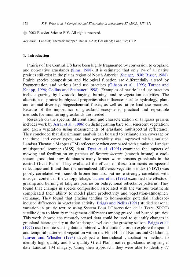
Comparison of Landsat TM and ERS-2 SARdata for discriminating among grassland types

and treatments in eastern Kansas

Kevin P. Price a,�, Xulin Guo a,1, James M. Stiles b

a Kansas Applied Remote Sensing Program, Department of Geography, University of Kansas, 2335 Irving

Hill Road, Lawrence, KS 66045, USAb Radar Systems and Remote Sensing Laboratory, Electrical Engineering and Computer Science, University

of Kansas, 2335 Irving Hill Road, Lawrence, KS 66045, USA

Abstract

The tallgrass prairies of North America are among the most biologically diverse grasslands

in the world. The way these lands are managed can have significant impacts on the biophysical

and compositional structure of plant and animal communities. Soil stability and other

hydrologic factors are also affected by grassland utilization practices. To better understand

how changing grassland management practices are impacting their respective ecosystems, we

must be able to map and monitor changing land use practices over large geographic areas. We

examined the potential of multitemporal Landsat Thematic Mapper (TM) and ERS-2

Synthetic Aperture Radar (SAR) imagery, and the combination of these two data sources

for discriminating among three commonly used tallgrass land management practices in areas

dominated by cool- and warm-season grass species in eastern Kansas. Our results showed that

cool- and warm-season grasses could be discriminated with 90.1% accuracy using the TM data

and 73.2% using the SAR data. The three grassland management practices were correctly

classified 70.4% of the time using TM data and 39.4% using SAR data. When TM and SAR

data were combined, the information contribution by SAR data to the discrimination of

grasslands was statistically insignificant. From our findings, we believe Landsat TM data can

be used to discriminate among various grassland types at a level of accuracy suitable for land

use change monitoring and assessing the impacts of changing government land use policies

such as the US Department of Agriculture’s Conservation Reserve Program (CRP).

� Corresponding author

E-mail address: [email protected] (K.P. Price).1 Present address: Department of Geography, University of Saskatchewan, Saskatoon, Saskatchewan,

Canada S7N 5A5.

Computers and Electronics in Agriculture 37 (2002) 157�/171

www.elsevier.com/locate/compag

0168-1699/02/$ - see front matter # 2002 Elsevier Science B.V. All rights reserved.

PII: S 0 1 6 8 - 1 6 9 9 ( 0 2 ) 0 0 1 1 0 - 2

mailto:[email protected]

# 2002 Elsevier Science B.V. All rights reserved.

Keywords: Landsat; Thematic mapper; Radar; SAR; Grassland; Land use; CRP

1. Introduction

Prairies of the Central US have been highly fragmented by conversion to cropland

and non-native grasslands (Sims, 1988). It is estimated that only 1% of all native

prairies still exist in the plains region of North America (Steiger, 1930; Risser, 1988).

Prairie species composition and biological function are differentially altered by

fragmentation and various land use practices (Gibson et al., 1993; Turner and

Knapp, 1996; Collins and Steinauer, 1998). Examples of prairie land use practices

include grazing by livestock, haying, burning, and re-vegetation activities. The

alteration of prairie biophysical properties also influences surface hydrology, plant

and animal diversity, biogeochemical fluxes, as well as future land use practices.

Because of the importance of grassland ecosystems, practical and repeatable

methods for monitoring grasslands are needed.

Research on the spectral differentiation and characterization of tallgrass prairies

includes work by Asrar et al. (1986) on distinguishing bare soil, senescent vegetation,

and green vegetation using measurements of grassland multispectral reflectance.

They concluded that discriminant analysis can be used to estimate area coverage by

the three land cover types, and that separability was improved with simulated

Landsat Thematic Mapper (TM) reflectance when compared with simulated Landsat

multispectral scanner (MSS) data. Dyer et al. (1991) examined the impacts of

mowing and fertilization on patches of Bromus inermis (smooth brome), a cool-

season grass that now dominates many former warm-seasons grasslands in the

central Great Plains. They evaluated the effects of these treatments on spectral

reflectance and found that the normalized difference vegetation index (NDVI) was

poorly correlated with smooth brome biomass, but more strongly correlated with

nitrogen content in the canopy foliage. Turner et al. (1992) examined the effects of

grazing and burning of tallgrass prairies on bidirectional reflectance patterns. They

found that changes in species composition associated with the various treatments

complicated their ability to model plant productivity and vegetation-atmosphere

exchange. They found that grazing tending to homogenize potential landscape-

induced differences in vegetation activity. Briggs and Nellis (1991) studied seasonal

variation in prairie texture using System Pour l’Observation de la Terre (SPOT)

satellite data to identify management differences among grazed and burned prairies.

This work showed the remotely sensed data could be used to quantify changes in

grassland heterogeneity at the landscape level over the growing season. Briggs et al.

(1997) used remote sensing data combined with abiotic factors to explore the spatial

and temporal patterns of vegetation within the Flint Hills of Kansas and Oklahoma.

Lauver and Whistler (1993) developed a hierarchical classification method to

identify high quality and low quality Great Plains native grasslands using single-

date Landsat TM imagery. Using their approach, they were able to identify 77

K.P. Price et al. / Computers and Electronics in Agriculture 37 (2002) 157�/171158

previously unknown native grassland areas. Price et al. (1993) found year-to-year

variation in precipitation patterns and land management practices to significantly

impact the spectral separability among six grassland types at an ecological reserve in

eastern Kansas.

The integration of multiple remote sensing data types for improved classification

has been examined by various investigators. Ulaby et al. (1982) found that the

combination of airborne radar with MSS data improved classification of Kansas’croplands by 10%. Brisco and Brown (1995) found that adding multi-temporal

Synthetic Aperture Radar (SAR) data to multi-temporal TM data improved

classification of western Canada croplands only slightly (from 90 to 92%). Haack

and Slonecker (1994) found that the combination of TM and the Spaceborne

Imaging Radar-B (SIR-B) data improved their ability to identify urban, vegetation,

and bare soils in the Sudan. Their overall classification accuracy was 94.1%. Haack

and Bechdol (1999) found that combining TM with RADARSAT and SIR-C radar

data slightly improved the classification accuracy for natural vegetation land covermapping in East Africa. Wang et al. (1998) examined the use of multi-date European

Remote Sensing Satellite-1 (ERS-1) SAR data and a single date of TM data for

classification of wetlands in Ontario, Canada. They achieved 97% classification

accuracy using the single-date TM imagery, and 80% accuracy using a combination

of five dates of radar data. Schadt et al. (1993) found better results from the use of

multi-temporal ERS-1 radar data than multi-temporal TM data for classifying

grasslands in Munich, Germany.

Previous studies have shown mixed results with respect to the benefits ofcombining optical and radar data. A majority of these studies have focused on

cropland discrimination. The objective of this study, therefore, was to assess the

spectral separability of warm- and cool-season grasslands under three management

practices with various combinations of multi-temporal Landsat TM and ERS-2 SAR

data.

2. Study area and methods

2.1. Study area

The study area is Douglas County in eastern Kansas. Douglas County has a total

area of about 1228 km2 (474 miles2). Kansas, which is located in the geographic

center of the continental United States, has a mid continental temperate climate. The

county receives an average of 900 mm of precipitation per year, with 70% falling

during the growing season (April through September). The average annualtemperature for Douglas County is 13 8C with a mean low monthly temperature

of �/2 8C in January and a mean high monthly temperature of 26 8C in July. The

length of the average growing season for the study area (frost-free period) is 185 days

(USDA, 1977). Climatic conditions in 1997 were similar to the mean for the last 30

years (Guo et al., 2000).

K.P. Price et al. / Computers and Electronics in Agriculture 37 (2002) 157�/171 159

Prior to early European settlement in the area, native grasses were the dominant

vegetation types. In 1990, the native and non-native grasslands covered 41% (50 335

ha) of the county (Whistler et al., 1995). The remaining land-cover types in the

county, in their respective order of dominance, were croplands (41%), woodlands

(12%), urban (3%), and water (3%). Grasses in the county include warm-season (C4

photosynthetic pathway) and cool-season (C3 photosynthetic pathway) species. The

dominant warm-season grasses include big bluestem (Andropogon gerardii Vitman.),little bluestem (Andropogon scoparius Michx.), Indiangrass (Sorghastrum nutans ),

and switchgrass (Panicum virgatum L.). The dominant cool-season grasses are

smooth brome (B. inermis Leyss.), tall fescue (Festuca arundinacia Schreb.),

Kentucky bluegrass (Poa pratensis L.), and orchardgrass (Dactylis glomerata L.).

The haying of cool-season grasslands in Douglas County normally takes place in

mid- to late-June. The haying of warm-season grasslands normally takes place in

mid-July to mid-August, but some are hayed as late as September. Cattle and some

horses are the predominant livestock grazers that are placed in grass pastures in thecounty. The normal stocking rate is about one cow per acre (Peterson, 1999). The

cattle are normally placed in the pastures sometime in May, and removed by mid- to

late-July. In years, when late summer soil moisture is sufficient to support a strong

resurgence of cool-season grasses, livestock may be moved back onto a pasture in

late summer.

The Conservation Reserve Program (CRP) was instituted under the 1985 US

Food Security Act and has as its primary objective the reduction of soil erosion in

areas where crops are grown on highly erodible soils. In Kansas, 1 170 034 ha ofcroplands have been converted to CRP (USDA, 1995) since 1985, increasing total

acreage in grassland by 14% (Wildlife Legacy Partners, 1994). Many Kansas counties

converted up to the maximum of 25% of their croplands to CRP. In the study area,

most CRP lands were reseeded to a native grass mixture that includes big bluestem,

little bluestem, switchgrass, and Indiangrass. To a much lesser degree, some CRP

lands were planted to pure stands of smooth brome, which is a common cool-season

pasture grass that is planted throughout the study area. Under normal circum-

stances, burning, mowing, and noxious weed control are the only land managementpractices permitted on CRP lands.

2.2. Field data collection

Seventy-one field sites were located using a random selection approach. This

approach involved the random identification of road intersections from which the

closest field site for each of the six grassland types was selected for subsequent field

data collection. Field sites were limited to areas large enough that a 3�/3 (90�/90 m)

cluster of Landsat TM pixels could be confidently positioned within a homogenouscovering of the grassland type. The number of field sites ultimately used in the

statistical analysis varied among grassland types because of isolated cumulus cloud

cover that obscured some field sites in the May and September TM images. As a

result, the sample sizes for each grassland type were as follows: 11 (warm-season

CRP (WC)), 13 (warm-season grazed (WG)), 12 (warm-season hayed (WH)), 11


(cool-season CRP (CC)), 12 (cool-season grazed (CG)), 12 (cool-season hayed

(CH)). The land use practice was confirmed through interviews with land owners.

The geographic location of each site was determined using Universal Transverse

Mercator (UTM) coordinates with a hand held global positioning system receiver.

The positional accuracy of each site was confirmed by overlaying the site locations

onto a 7.5-min orthophotoquadrangle. This conformation process identified several

positional errors that were most likely due to incorrect data entry of the geographiccoordinates. All locations were corrected before the positional data were used in the

subsequent data extraction process described later.

At each field site location, biophysical data were collected in late spring and mid-

summer of 1997. The field sampling period was designed to coincide with the May

and July satellite overpasses as closely as possible (approximately 2 weeks before and

after the overflight dates). Ocular estimates of forb and grass cover (%) were

collected in both May and July, and aboveground dry biomass (hereafter, ‘biomass’)

(g/m2) (n�/40) was collected between May and July. Dry biomass was measuredwithin five 0.25 m2 quadrats in each 90�/90 m study plot. Covers were estimated

within these quadrats as well. Because of time constraints, biomass could be collected

only at 40 of the 69 sites. Plant moisture content (g/m2) was calculated from the

difference between wet and dry biomass. Species richness data were collected by

counting species of grasses, forbs, shrubs, and trees in each study plot.

The sites were classified as cool- or warm-season based on the dominant plant

species found at each site. A prevalent�/frequency (P �/F ) index (Curtis, 1959;

Warner and Harper, 1972) was computed to rank each species according to itsfrequency within, and prevalence across all sites. The P �/F index was calculated by

multiplying the percentage of the presence of each plant species among all sites by

the percentage of the frequency of all species within the five 0.25 m2 quadrats used to

estimate vegetation cover. P �/F index values ranged from 0.0 (the species is not

present in any plot) to 10 000 (the species is 100% present at all sites and found in

100% of all quadrats at each site).

2.3. TM and SAR data acquisition and preprocessing

Three nearly cloud-free Landsat-5 TM images (path 27, row 33) that covered the

study area were acquired for the following dates: 15 May (late spring), 2 July

(midsummer), and 4 September (late summer), 1997. After each image was examined

for sensor errors (i.e. striping, banding, line dropout), the digital numbers were then

converted to radiance using the method described by Markham and Barker (1986).

The reflectance values were adjusted for atmospheric scatter using the improved

dark object subtraction technique described by Chavez (1988). The images were

corrected for geometric error by first transforming the July image to a UTMprojection. The geometric transformation equation was computed using 38 ground

control points that produced a final root mean square (RMS) error of B/0.35 pixels

(B/10.5 m). The May and September images then were georegistered to the ground-

rectified July image. The spectral values for each pixel were interpolated using a

nearest-neighbor resampling approach and the data were output to a 30�/30 m pixel


size. During the geometric correction process, the images were clipped to the

Douglas County political boundary and the thermal band was eliminated from each

image, resulting in an 18-band dataset (six bands for each date). The six Landsat TM

bands and their associated wavelengths used in this study include: band 1 (blue�/

green, 450�/520 nm), band 2 (green, 520�/600 nm), band 3 (red, 630�/690 nm), band 4

(near infrared (NIR), 760�/900 nm), band 5 (middle infrared (MIR), 1550�/1750 nm),

and band 7 (middle infrared, 2080�/2350 nm).Four ERS-2 SAR images covering the study area were acquired for 21 May, 25

June, 3 September, and 8 October, 1997. Significant rainfall events were recorded at

the Douglas County meteorological station just prior to image acquisitions in June

(33 mm) and October (22 mm). These dates were selected to match the TM image

overflight dates as closely as possible. The ERS-2 SAR sensor collects data in the C-

band (5.3 Ghz, 5.565 cm) region of the spectrum. We used the ERS-2 SAR precision

image (PRI) format, which is the Europe Space Agency standard product for SAR

radiometric precision analysis. The image pixel values are linearly proportional toradar brightness, a value that is in turn proportional to the backscattering coefficient

divided by the sine of the pixel incidence angle. ERS-2 images are corrected for the

in-flight elevation antenna pattern and compensated for range spreading loss (Laur

et al., 1998). Thus, the scenes are calibrated in a relative sense across the spatial

extent of the image. ERS-2 images, however, are not calibrated in a absolute sense,

so the absolute values of the pixels intensities (e.g. backscattering coefficients) are

not provided. Because the objective of this study was to test the potential of

multitemporal radar data for discriminating among grassland types, the use of arelative calibration was deemed sufficient to discriminate between dissimilar

vegetation types within the study area.

Speckle within the SAR images was minimized using the median of values within a

3�/3 window. Fifteen ground control points were collected throughout the study

area and used to develop the geometric transformation equations that resulted in a

RMS error of B/0.5 pixels (B/6.25 m). The radar brightness for each pixel was

interpolated using a nearest neighbor resampling approach and the pixels were

scaled to the original sensor resolution of 12.5�/12.5 m, as well as 30�/30 mresolution to match the spatial resolution of TM imagery.

2.4. Statistical analysis

The geographic locations of the 71 study plots were overlaid onto the 18-band TM

and 4-band SAR data set using a GIS overlay procedure. At each location, the

reflectance values of the nine closest pixels (3�/3 pixel area) were used to estimate

the spectral reflectance mean and variance associated with each plot. For the SAR

data, the mean and variance of the radar pixel values were calculated using the 49pixel values (7�/7 pixels) closest to each field site location. The 7�/7 pixel (87.5�/

87.5 m) sample was used for the SAR 12.5 m resolution data to approximate the

same area as sampled for the 3�/3 pixel (90�/90 m) TM data. The 3�/3 pixel

sample size was used for the SAR 30�/30 m resolution data. Multiple analysis of

variance (MANOVA) tests were used to determine whether significant biophysical


and spectral differences existed among grassland types and management practices at

0.05 significance level.

Discriminate analysis was used to test the spectral separability among grassland

types. The discriminant functions were used to classify each site into various

grassland categories (e.g. cool- vs. warm-season grassland or grazed, hayed, and

CRP, etc.). According to Congalton and Green (1998), at least 50 samples for each

category should be used to evaluate classification accuracy. Due to the small samplesize (an unavoidable constraint because of the few remaining warm-season grassland

sites in the region) associated with each grassland type, the accuracy of our

discriminant function classification was tested using a Jack-Knife cross validation

(JCV) approach. This approach was implemented by withholding the spectral data

for one site and building the discriminant functions using the data from the

remaining sites. The process of removing one site from the dataset was repeated until

all sites had been withheld. User and producer classification accuracy and the Khat

statistic were also evaluated using the methods described by Congalton and Green(1998). Measurements of producer error indicate the chances of underestimating

(errors of omission) a particular cover class, while measurements of user error

indicate the chance of overestimating (errors of commission) a particular class. The

Khat statistic is used to estimate k (kappa), which is a ‘measure of the difference

between the observed agreement between two maps (as reported by the diagonal

entries in the error matrix) and the agreement that might be attained solely by chance

matching of the two maps’ (Campell, 1996).

3. Results and discussion

3.1. Dominate and sub-dominate species for each grassland types

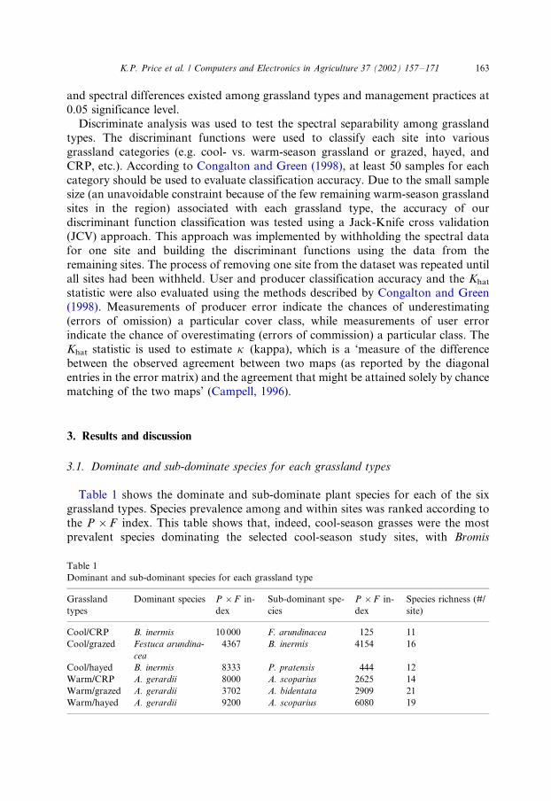
Table 1 shows the dominate and sub-dominate plant species for each of the six

grassland types. Species prevalence among and within sites was ranked according to

the P �/F index. This table shows that, indeed, cool-season grasses were the most

prevalent species dominating the selected cool-season study sites, with Bromis

Table 1

Dominant and sub-dominant species for each grassland type

Grassland

types

Dominant species P �/F in-

dex

Sub-dominant spe-

cies

P �/F in-

dex

Species richness (#/

site)

Cool/CRP B. inermis 10 000 F. arundinacea 125 11

Cool/grazed Festuca arundina-

cea

4367 B. inermis 4154 16

Cool/hayed B. inermis 8333 P. pratensis 444 12

Warm/CRP A. gerardii 8000 A. scoparius 2625 14

Warm/grazed A. gerardii 3702 A. bidentata 2909 21

Warm/hayed A. gerardii 9200 A. scoparius 6080 19


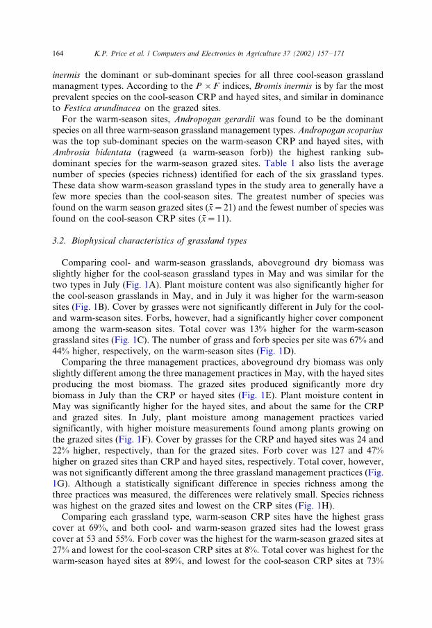
inermis the dominant or sub-dominant species for all three cool-season grassland

managment types. According to the P �/F indices, Bromis inermis is by far the most

prevalent species on the cool-season CRP and hayed sites, and similar in dominance

to Festica arundinacea on the grazed sites.

For the warm-season sites, Andropogan gerardii was found to be the dominant

species on all three warm-season grassland management types. Andropogan scoparius

was the top sub-dominant species on the warm-season CRP and hayed sites, withAmbrosia bidentata (ragweed (a warm-season forb)) the highest ranking sub-

dominant species for the warm-season grazed sites. Table 1 also lists the average

number of species (species richness) identified for each of the six grassland types.

These data show warm-season grassland types in the study area to generally have a

few more species than the cool-season sites. The greatest number of species was

found on the warm season grazed sites (/x/�/21) and the fewest number of species was

found on the cool-season CRP sites (/x/�/11).

3.2. Biophysical characteristics of grassland types

Comparing cool- and warm-season grasslands, aboveground dry biomass was

slightly higher for the cool-season grassland types in May and was similar for the

two types in July (Fig. 1A). Plant moisture content was also significantly higher for

the cool-season grasslands in May, and in July it was higher for the warm-season

sites (Fig. 1B). Cover by grasses were not significantly different in July for the cool-

and warm-season sites. Forbs, however, had a significantly higher cover component

among the warm-season sites. Total cover was 13% higher for the warm-seasongrassland sites (Fig. 1C). The number of grass and forb species per site was 67% and

44% higher, respectively, on the warm-season sites (Fig. 1D).

Comparing the three management practices, aboveground dry biomass was only

slightly different among the three management practices in May, with the hayed sites

producing the most biomass. The grazed sites produced significantly more dry

biomass in July than the CRP or hayed sites (Fig. 1E). Plant moisture content in

May was significantly higher for the hayed sites, and about the same for the CRP

and grazed sites. In July, plant moisture among management practices variedsignificantly, with higher moisture measurements found among plants growing on

the grazed sites (Fig. 1F). Cover by grasses for the CRP and hayed sites was 24 and

22% higher, respectively, than for the grazed sites. Forb cover was 127 and 47%

higher on grazed sites than CRP and hayed sites, respectively. Total cover, however,

was not significantly different among the three grassland management practices (Fig.

1G). Although a statistically significant difference in species richness among the

three practices was measured, the differences were relatively small. Species richness

was highest on the grazed sites and lowest on the CRP sites (Fig. 1H).Comparing each grassland type, warm-season CRP sites have the highest grass

cover at 69%, and both cool- and warm-season grazed sites had the lowest grass

cover at 53 and 55%. Forb cover was the highest for the warm-season grazed sites at

27% and lowest for the cool-season CRP sites at 8%. Total cover was highest for the

warm-season hayed sites at 89%, and lowest for the cool-season CRP sites at 73%


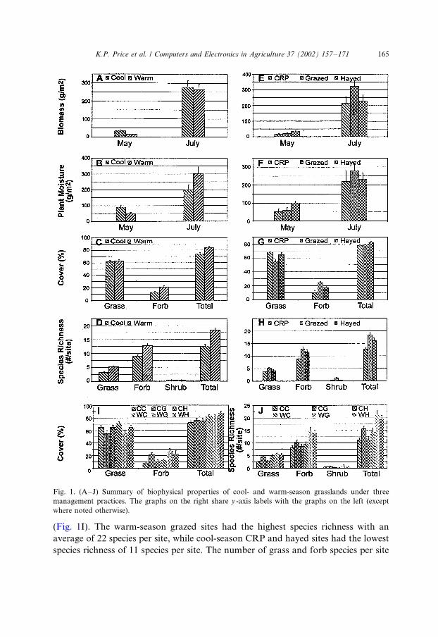
(Fig. 1I). The warm-season grazed sites had the highest species richness with an

average of 22 species per site, while cool-season CRP and hayed sites had the lowest

species richness of 11 species per site. The number of grass and forb species per site

Fig. 1. (A�/J) Summary of biophysical properties of cool- and warm-season grasslands under three

management practices. The graphs on the right share y -axis labels with the graphs on the left (except

where noted otherwise).


varied considerably among the six practices. A few shrub species were found within a

few plots among the six practices. (Fig. 1J).

3.3. Spectral discrimination of cool- and warm-season grasslands

The results of the discriminant analysis showed that cool- and warm-season

grasslands could be spectrally discriminated with 90.1% accuracy using the

combination of the three TM images. Using the four dates of SAR data, these

same grasslands could be discriminated with 73.2% accuracy. The Khat statistics

showed that after adjusting for producer and user errors, the discrimination accuracy

of the grassland types was 80.0% using the TM data, and 46.2% using the SAR data.Price et al. (1999) concluded that the reason for the improved discrimination among

these two life-forms was due to differences in phenology of the cool- and warm-

season plants. This is because cool-season plants become photosynthetically active

earlier in the growing season when temperatures are much cooler, and become active

again in the fall after temperures decrease. The amount of fall regrowth is

constrained by soil moisture availability. The warm-season grasses, on the other

hand, grow most rapidly during the summer when temperatures are hot and soil

surface moisture is often more limited. We found that the differences in thephenological growth patterns of cool- and warm-season grasses were the key to

spectrally discriminating grasslands based on life-form differences.

3.4. Spectral discrimination among grassland management practices

The results of the discriminant analysis showed that grasslands under CRP,

grazing, and haying management practices could be spectrally discriminated with

70.4% accuracy using the three TM images, and with 39.4% accuracy when the SAR

data alone were used. The Khat statistics showed that after adjusting for producer

and user errors, the discrimination of the grassland management types was 55.5% for

the TM data, and 9.0% for the SAR data. Among these three management practices,

hayed sites were less accurately discriminated because of its variability in hayingactivity. The producer’s and user’s discriminating accuracies were 61.5 and 66.7% for

hayed sites, respectively, which were lower than the discriminating accuracies of

CRP and grazed sites. The producer’s and user’s discriminating accuracies were 75.0

and 68.2% for CRP sites, respectively, and 76.0% for grazed sites for both the user’s

and producer’s accuracies.

We also evaluated the spectral separability of the six grassland management

practices (cool- and warm-season CRP, grazed, and hayed). The results showed that

the six management practices could be spectrally discriminated with 63.4% accuracyusing the three TM images, and with 26.8% accuracy when only the SAR data were

used (Table 2). The Khat statistics showed that after adjusting for producer and user

errors, the discrimination of the six types was 56.0% for the TM data, and 12.2% for

the SAR data. Results also showed that CRP sites were most accurately classified

among all the grassland management practices (Table 2).


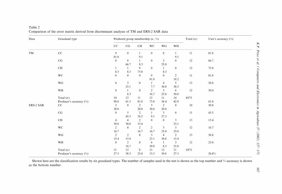
Table 2

Comparison of the error matrix derived from discriminant analyses of TM and ERS-2 SAR data

Data Grassland type Predicted group membership (n , %) Total (n ) User’s accuracy (%)

CC CG CH WC WG WH

TM CC 9 0 1 0 0 1 11 81.8

81.8 9.1 9.1

CG 0 8 1 0 3 0 12 66.7

66.7 8.3 25.0

CH 1 1 9 0 1 0 12 75.0

8.3 8.3 75.0 8.3

WC 0 0 0 9 0 2 11 81.8

81.8 18.2

WG 0 3 0 1 4 5 13 30.8

23.1 7.7 30.8 38.5

WH 0 1 0 2 3 6 12 50.0

8.3 16.7 25.0 50.0

Total (n ) 10 13 11 12 11 14 45/71

Producer’s accuracy (%) 90.0 61.5 81.8 75.0 36.4 42.9 63.4

ERS-2 SAR CC 3 0 2 3 2 0 10 30.0

30.0 20.0 30.0 20.0

CG 0 5 2 1 3 0 11 45.5

45.5 18.2 9.1 27.3

CH 4 4 2 0 0 3 13 15.4

30.8 30.8 15.4 23.1

WC 2 0 2 2 3 3 12 16.7

16.7 16.7 16.7 25.0 25.0

WG 2 2 0 3 4 2 13 30.8

15.4 15.4 23.1 30.8 15.4

WH 0 2 0 6 1 3 12 25.0

16.7 50.0 8.3 25.0

Total (n ) 11 13 8 15 13 11 19/71

Producer’s accuracy (%) 27.3 38.5 25.0 13.3 30.8 27.3 26.8%

Shown here are the classification results by six grassland types. The number of samples used in the test is shown as the top number and % accuracy is shown

as the bottom number.

K.P

.P

riceet

al.

/C

om

pu

tersa

nd

Electro

nics

inA

gricu

lture

37

(2

00

2)

15

7�

/17

11

67

When management practices were stratified by cool- and warm-season grasslands,

the grazed types were most difficult to spectrally discriminate (Table 2). We

hypothesize that this is because cool-season grasslands are typically hayed earlier

than are warm-season grasslands. When cool- and warm-season types are classified

together, there is greater spectral variation associated with hayed grassland types.

The spectral separability associated with the SAR data, however, showed that the

grazed grasslands were most spectrally distinct among the management practices,

but TM data still were the best discriminator of the grazed sites. A possible

explanation for this finding lies in the unique characteristics of the underlying soil of

grazed surfaces compared with those that are not grazed. For example, Price et al.

(1993) found that soil moisture was consistenly lower for grazed warm-season

grassland sites when compared with other grassland management practices in their

study area. Also, one might speculate that surface roughness of grazed sites would be

greater because of the constant trampling by the hooves of livestock and soil

moisture holding capacity lower because of increased soil compaction. Numerous

studies have documented the sensitivity of the C-band on the ERS-2 SAR system to

varying soil moisture and surface roughness conditions (i.e. Weimann et al. 1998).

The ability of the C-band to penetrate through the grass and forb canopy to detect

differences in soil moisture and roughness conditions might explain why the SAR

data could most accurately discriminate the grazed sites from among the other

management practices. Additional field measurements are needed, however, to

confirm that there are differences in surface roughness between grazed grasslands

compared with the other management types.

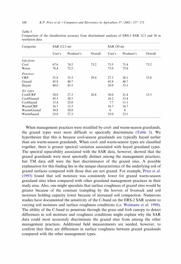
Table 3

Comparison of the classification accuracy from discriminant analyses of ERS-2 SAR 12.5 and 30 m

resolution data

Categories SAR (12.5 m) SAR (30 m)

User’s Producer’s Overall User’s Producer’s Overall

Life-form

Cool 67.6 74.2 73.2 73.5 71.4 73.2

Warm 78.4 72.5 73.0 75.0

Practices

CRP 31.8 33.3 39.4 27.3 26.1 33.8

Grazed 45.8 40.7 45.8 40.7

Hayed 40.0 43.5 28.0 33.3

Six types

Cool/CRP 30.0 27.3 26.8 30.0 21.4 15.5

Cool/Garzed 45.5 38.5 18.2 15.4

Cool/hayed 15.4 25.0 7.7 11.1

Warm/CRP 16.7 13.3 16.7 16.7

Warm/Grazed 30.8 30.8 0 0

Warm/hayed 25.0 27.3 25.0 23.1


3.5. Combination of TM and SAR data classification

TM and SAR data were combined to evaluate the utility of integrating the two

data typed for discriminating among the cool- and warm-season grasslands, the three

management practices irrespective of life-form, and the six grassland types when

management practices were stratified by life-form. When the three dates of TM data

were combined with the four dates of SAR data, the classification accuracies were88.4, 69.6, an 59.4% for discriminating life-forms, management practices, and six

grassland types, respectively, which were 1.7, 0.8, and 4.0% less accurate than when

only TM data were used. Therefore, combining TM and SAR data did not improve

separability of grassland types in our study area.

We also compared the SAR data resampled to 12.5 and 30 m resolution to

determine whether resampling the SAR data to the same resolution as the TM data

had any impact on classification accuracy. The results of this comparison are listed

in Table 3. We found that the use of 30 m pixel size did not change the classificationaccuracy of the life-form classes, and the accuracy decreased when the 30 m pixel size

was use to classify the management practices.

4. Conclusion

Both TM and ERS-2 SAR data were used to separate grassland types with varying

degrees of accuracy. The TM data were 14% to 31% more accurate than the SARdata for discriminating among the grassland types that were evaluated in this study.

We found that the inclusion of ERS-2 SAR data did not significantly improve

classification accuracy of grassland management types. ERS-2 is a single channel

radar system, while TM provides seven channels of spectral data. Multichannel

radar, such as the one flown on the Shuttle Imaging Radar (SIR-C) mission,

provides backscattering data for multiple frequencies and polarization. These

sensors have demonstrated significantly greater classification performance over

that of single-channel systems (Stofan et al., 1995). A multi-channel SAR mightprovide more useful data for grassland classification.

From our findings, we believe Landsat TM data can be used to discriminate

among various grassland types at a level of accuracy suitable for land use change

monitoring and assessing the impacts of changing government land use policies such

as the US Department of Agriculture’s CRP. Such measurements will provide

valuable input to ecosystem and biogeochemical models that are needed to study

human and natural induced ecosystem changes and their impacts on plant and

animal dynamics and biogeochemical cycles.

Acknowledgements

This study was supported through the Kansas NASA EPSCoR Project and the

Kansas Applied Remote Sensing (KARS) Program and Department of Geography,


University of Kansas. Additional support was provided by the NASA Earth Science

Enterprise, Earth Science Applications Research Program (ESARP). This work was

being conducted in cooperation with the Department of Geography at Kansas State

University and the Earth Science Department at Emporia State University. We wish

to thank Ina Robertson and Dana Peterson for their contribution to the collection of

field data.

References

Asrar, G., Weiser, R.L., Johnson, D.E., Kanemasu, E.T., Killeen, J.M., 1986. Distinguishing among

tallgrass prairie cover types from measurements of multispectral reflectance. Remote Sensing of

Environment 19, 159�/169.

Briggs, J.M., Nellis, M.D., 1991. Seasonal variation of heterogeneity in tallgrass prairie: a quantitative

measure using remote sensing. Photogrammetric Engineering and Remote Sensing 55, 407�/411.

Briggs, J.M., Rieck, D.R., Turner, C.L., Henebry, G.M., Goodin, D.G., Nellis, M.D., 1997. Spatial and

temporal patterns of vegetation within the Flint Hills. Transactions of the Kansas Academy Science

100, 10�/20.

Brisco, B., Brown, R.J., 1995. Multidate SAR/TM synergism for crop classification in western Canada.

Photogrammetric Engineering and Remote Sensing 61, 1009�/1014.

Campell, J.B., 1996. Introduction to Remote Sensing, second ed.. The Guilford Press, New York, p. 622.

Chavez, P.S., 1988. An improved dark-object subtraction technique for atmospheric scattering correction

of multispectral data. Remote Sensing of Environment 24, 459�/479.

Collins, S.L., Steinauer, E.M., 1998. Disturbance, diversity, and species interactions in tallgrass prairie. In:

Grassland Dynamics. Oxford University Press, New York, NY, pp. 140�/156.

Congalton, R.G., Green, K., 1998. Assessing the Accuracy of Remotely Sensed Data: Principles and

Practices. Lewis Publishers, New York, NY, p. 180.

Curtis, J.T., 1959. The Vegetation of Wisconsin. University of Wisconsin Press, Madison, WI.

Dyer, M.I., Turner, C.L., Seastedt, T.K., 1991. Mowing and fertilization effects on productivity and

spectral reflectance in Bromus inermis plots. Ecological Applications 1, 443�/452.

Gibson, D.J., Seastedt, T.R., Briggs, J.M., 1993. Management practices in tallgrass prairie: large- and

small-scale experimental effects on species composition. Journal of Applied Ecology 30, 247�/255.

Guo, X., Price, K.P., Stiles, J.M., 2000. Modeling biophysical factors for grasslands in eastern Kansas

using Landsat TM data. Kansas Academic Science Transaction 103, 122�/138.

Haack, B., Slonecker, E., 1994. Merged spaceborne radar and Thematic Mapper digital data for locating

villages in Sudan. Photogrammetric Engineering and Remote Sensing 60, 1253�/1257.

Haack, B., Bechdol, M., 1999. Land cover mapping using radar, radar texture and optical data

intergration. In: Proceedings of American Society of Photogrammetry and Remote Sensing, Portland,

OR.

Laur, H., Bally, P., Meadows, P., Sanchez, J., Schaettler, B., Lopinto, E., Esteban, D., 1998. ERS SAR

calibration: Derivation of backscattering coefficient sigma-nought in ESA ERS SAR PRI products,

ESA/ESRIN, Issue 2, Rev. 5b. Document No: ES-TN-RS-PM-HL09 7 September 1998.

Lauver, C.L., Whistler, J.L., 1993. A hierarchical classification of Landsat TM imagery to identify natural

grassland areas and rare species habitat. Photogrammetric Engineering and Remote Sensing 59, 627�/

634.

Markham, B.L., Barker, J.L., 1986. Landsat MSS and TM post-calibration dynamic ranges, exoatmo-

spheric reflectances and at-satellite temperatures. EOSAT LANDSAT TECHNICAL NOTES,

August, p. 3�/8.

Peterson, D.L., 1999. Spectral characteristics of grazed native warm season and non-native cool season

grasslands in Douglas County, Kansas. Theses, University of Kansas, p. 120.


Price, K.P., Martinko, E.A., Rundquist, D.C., Peake, J.S., 1993. Influences of land management and

weather on plant biophysical and hyper-spectral response patterns of tallgrass prairies in northeastern

Kansas. In Proceedings of PECORA12, Sioux Falls, South Dakota, pp. 441�/450.

Price, K.P., Guo, X., Stiles, J.M., 1999. Discriminant analysis of Landsat TM multi-temporal data for six

grassland management practices in eastern Kansas. In: Proceedings of American Society of

Photogrammetry and Remote Sensing, Portland, OR.

Risser, P.G., 1988. In: Wilson, E.O. (Ed.), Diversity in and Among Grasslands, Biodiversity. National

Academy Press, Washington, DC, pp. 176�/180.

Schadt, R., Kellndorfer, J., Mauser, W., 1993. Comparison of ERS-1 SLC and Landsat Thematic Mapper

data for monitoring grassland and detecting changes in agricultural use. In: Proceedings of Second

ERS-1 Symposium-Space at the Service of Our Environment, Hamburg, Germany, pp. 75�/78.

Sims, P.L., 1988. In: Barbour, M.G., Billings, W.D. (Eds.), Grasslands, North America terrestrial

Vegetation. Cambridge University Press, New York, NY, pp. 266�/286.

Steiger, T.L., 1930. Structure of prairie vegetation. Ecology 11, 170�/217.

Stofan, E.R., Evans, D.L., Schmullius, C., Holt, B., Plaut, J.J., Vanzyl, J., Wall, S.D., Way, J., 1995.

Overview of results of Spaceborne Imaging Radar-C, X-band Synthetic Aperture Radar (SIR-C, X-

SAR). IEEE Transactions on Geoscience and Remote Sensing GE-33, 817�/828.

Turner, C.L., Knapp, A.K., 1996. Responses of a C4 grass and three C3 forbs to variation in nitrogen and

light in tallgrass prairie. Ecology 77, 1738�/1749.

Turner, C.L., Seastedt, T.R., Dyer, M.I., Kittel, T.G.F., Schimel, D.S., 1992. Effects of management and

topography on the radiometric response of a tallgrass prairie. Journal of Geophysical Research 97

(D17), 18855�/18866.

Ulaby, F.T., Li, R.Y., Shanmugan, K.S., 1982. Crop classification using airborne radar and Landsat data.

IEEE Transactions on Geoscience and Remote Sensing GE-20, 42�/50.

USDA, 1995. CRP Statistics from the Kansas State Farm Service, Manhattan, KS.

USDA, 1977. Soil survey of Douglas County: US Department of Agriculture, Soil Conservation Service in

Cooperation with Kansas Agricultural Experiment Station, Washington, DC, p. 73.

Wang, J., Shang, J., Brisco, B., Brown, R.J., 1998. Evaluation of multidate ERS-1 and multispectral

Landsat imagery for wetland detection in southern Ontario. Canadian Journal of Remote Sensing 24,

60�/68.

Warner, J.T., Harper, K.T., 1972. Understory characteristics related to site quality for Aspen in Utah.

Brigham Young University Science Bulletin, Biological Series 16, 1�/20.

Weimann, A., Schonermark, M.V., Schumann, A., Jorn, P., Gunther, R., 1998. Soil moisture estimation

with ERS-1 SAR data in the East-German loess soil area. International Journal of Remote Sensing 19,

237�/243.

Whistler, J.L., Egbert, S.L., Jakubauskas, M.E., Martinko, E.A., Baumgartner, D.W., Lee, R., 1995. The

Kansas State land mapping project: regional scale land use/land cover mapping using Landsat

Thematic Mapper data. In Technical Paper of ACSM/ASPRS Annual Convention and Exposition,

Charlotte, NC 3 773-785.

Wildlife Legacy Partners, 1994. The Conservation Reserve Program: a Wildlife Conservation Legacy,

Wildlife Management Institute, Washington, DC.


Documents

Comparison of Landsat TM and ERS-2 SAR data for discriminating among grassland types and treatments in eastern Kansas