Embed Size (px)
Citation preview
Comparison of EC-Kit with Quanti-Tray®:
Testing, Verification, and Drinking Water Quality Mapping
in Capiz Province, Philippines
By
Patty Chuang
BS, Environmental Sciences and Engineering, Mathematics
Gillings School of Global Public Health
The University of North Carolina at Chapel Hill, NC 2009
Submitted to the Department of Civil and Environmental Engineering
in partial fulfillment of the requirements for the degree of
Master of Engineering in Civil and Environmental Engineering
at the
MASSACHUSETTS INSTITUTE OF TECHNOLOGY
June 2010
© 2010 Patty Chuang. All rights reserved.
The author hereby grants to MIT permission to reproduce and to distribute publicly
paper and electronic copies of this thesis document in whole or in part in any medium
now known or hereafter created.
Signature of Author: _________________________________________________________
Patty Chuang
Department of Civil and Environmental Engineering
May 21, 2010
Certified by: _______________________________________________________________
Susan Murcott
Senior Lecturer of Civil and Environmental Engineering
Thesis Supervisor
Accepted by: _______________________________________________________________
Daniele Veneziano
Chairman, Departmental Committee for Graduate Students

Comparison of EC-Kit with Quanti-Tray®:
Testing, Verification, and Drinking Water Quality Mapping
in Capiz Province, Philippines
By:
Patty Chuang
Submitted to the Department of Civil and Environmental Engineering
on May 21, 2010 in Partial Fulfillment of the
Requirements for the Degree of Master of Engineering in
Civil and Environmental Engineering
ABSTRACT
This thesis accomplishes three tasks. First, it verifies the EC-Kit under different water
source conditions by comparing it to a laboratory standard method, the IDEXX Quanti-Tray®.
The EC-Kit is a simple, inexpensive field test kit that contains complementary tests for
Escherichia coli and total coliform: the Colilert® 10-milliliter presence/absence test and 3MTM
’s
PetrifilmTM
test. This work was executed by analyzing 521 water samples collected in Capiz
Province, Philippines as well as 40 water samples from the Charles River in Cambridge,
Massachusetts. Second, it determines the risk level for drinking water sources according to
E.coli and total coliform levels in Capiz Province for difference locations and source types.
Third, this study contributes to an ongoing mapping project, aimed at creating an interactive,
searchable map of water quality results from EC-Kit and Quanti-Tray®.
The results of the study reveal that each component of EC-Kit and the entire kit itself is
correlated to Quanti-Tray® in a statistically significant way. Moreover, from the calculations of
error and proportional reduction in error for unimproved/improved water sources, it is possible to
make better predictions with just the use of the Colilert® test, but not just the use of the
PetrifilmTM
. This is because the detection limits for PetrifilmTM
are an order of magnitude higher
than Colilert®, namely PetrifilmTM
colony counts of 1-10/1 mL sample results fall within the
High and colony counts of 10-100/1 mL of sample fall within the Very High risk level
categories, whereas positive Colilert® results fall within the Intermediate, High, and Very High
risk level categories. Most importantly, the EC-Kit allows for the best reduction in error, with a
proportional reduction in error of 63% for unimproved water sources and 60% for improved
water sources. This finding is significant because it means that a simple, inexpensive field kit
can change our understanding of the safety of drinking water compared to simply knowing the
United Nations infrastructure designation of improved versus unimproved water sources.
Furthermore, the statistical analyses revealed that while the EC-Kit does not exactly match the
Quanti-Tray® results, it still provides useful information for assessing at-risk water sources.
Thesis Supervisor: Susan Murcott
Title: Senior Lecturer, Civil and Environmental Engineering

4
ACKNOWLEDGEMENTS
I would like to express my most sincere thanks to:
Susan Murcott, my professor and thesis supervisor, for her expertise, guidance, and support
throughout the year. As one of my primary reasons for attending MIT, I am utterly grateful to
have been able to work with her in such close capacity. She is forever an inspiration.
Jarvis Punsalan and Jane Delos Reyes for their leadership in this project, and for showing the
beauty of Capiz Province. Many thanks to friends and staff from the Capiz Provincial Health
Office, without whom this entire project would have been impossible.
Ezra Glenn and Jonathan Lowe for their help and support in many technical aspects of this
report. Ezra, for his excellent teaching and methods of thinking about numbers and statistics in
an entirely new way. Jonathan, for his development of the GIS website and mapping, and
constant availability. In addition to breadth of knowledge, they have been incredibly kind and
giving in their assistance and time.
John Millspaugh, Molly Patrick, and Stephanie Trottier for being the best travel mates I could
have ever had in the Philippines. Fondly, I remember our times riding tricycles, eating at
Alma’s, fighting the giant rat and cockroach invasion of 2010, and lounging upon the sandy
beaches of Boracay Island.
Additionally, my complete and utter heartfelt thanks the fellow members of the CEE Masters of
Engineering program, for giving me the blessing of their friendship and company.
And most importantly, my parents, and Colleen Storey Vasu. Ma and Pa, I would never have
gotten this far without your perpetual support and sage advice. And Colleen, for being the truest
of friends, the Ron to my Harry and the Sam to my Frodo.

5
6
Table of Contents CHAPTER 1: INTRODUCTION .............................................................................................. 13
1.1 Background ..................................................................................................................... 14
1.2 Scope of Current Work .................................................................................................... 15
1.3 Overview of the Philippines ............................................................................................. 15
1.4 Water Use in the Philippines ............................................................................................ 17
1.5 Drinking Water Regulations in the Philippines ................................................................. 18
1.6 Overview of Capiz Province, Philippines ......................................................................... 20
CHAPTER 2: LITERATURE REVIEW ................................................................................... 23
2.1 Indicator Microorganisms ................................................................................................ 23
2.2 Overview of Microbial Assay Methods ............................................................................ 23
2.3 Quanti-Tray® and Quanti-Tray®/2000 ............................................................................ 24
2.4 EC-Kit ............................................................................................................................. 25
2.5 Studies on Colilert® Reagent ........................................................................................... 25
2.6 Studies on 3M PetrifilmTM
............................................................................................... 27
CHAPTER 3: RESEARCH AND SAMPLING DESIGN .......................................................... 30
3.1 Overview of Research and Sampling Design .................................................................... 30
3.2: Sample Collection........................................................................................................... 31
CHAPTER 4: METHODOLOGY ............................................................................................. 34
4.1 Procedure for Quanti-Tray® Test ..................................................................................... 34
4.2 Procedure for EC-Kit: Colilert® and PetrifilmTM
............................................................. 36
7
4.2.1 Procedure for Colilert® (10-mL Predispensed Tubes) ............................................... 37
4.2.2 Procedure for PetrifilmTM
Test .................................................................................. 39
4.2.3 Recommendations on Reading Colilert® and PetrifilmTM
Results ............................. 42
4.2.4 Determining Risk Levels from EC-Kit Results .......................................................... 43
4.3 Charles River Water Sampling ......................................................................................... 45
4.4 GPS Testing ..................................................................................................................... 46
4.5 Statistical Analyses .......................................................................................................... 47
4.6 Limitations to the Study ................................................................................................... 49
CHAPTER 5: EC-KIT COMPARISON TO QUANTI-TRAY® ................................................ 50
5.1 Colilert®/Quanti-Tray® Comparison and PetrifilmTM
/Quanti-Tray® Comparison for Capiz
Province Water Samples ........................................................................................................ 50
5.2 Colilert®/Quanti-Tray® Comparison and PetrifilmTM
/Quanti-Tray® Comparison for
Charles River Water Samples ................................................................................................ 51
5.3 EC-Kit (Combined Colilert® and PetrifilmTM
) and Quanti-Tray® Comparison Results for
Both Capiz Province and Charles River Water ....................................................................... 54
CHAPTER 6: ACCURACY OF EC-KIT IN REDUCING ERROR RELATIVE TO
IMPROVED/UNIMPROVED WATER SOURCE DESIGNATION ......................................... 56
CHAPTER 7: DRINKING WATER QUALITY AND RISK LEVELS ..................................... 59
CHAPTER 8: DRINKING WATER QUALITY MAPPING ..................................................... 62
CHAPTER 9: CONCLUSION AND RECOMMENDATIONS ................................................. 64
9.1 EC-Kit Verification and Testing ...................................................................................... 64
9.2 Drinking Water Quality Mapping..................................................................................... 64
8
9.3 Summary ......................................................................................................................... 64
9.4 Recommendations for Future Studies ............................................................................... 65
CHAPTER 10: REFERENCES ................................................................................................. 67
APPENDICES .......................................................................................................................... 71
Appendix A: IDEXX 51-Well Quanti-Tray® MPN Table ...................................................... 72
Appendix B: Water Quality Results, Sorted by Municipality ................................................. 75
Appendix C: Charles River Water Quality Results ............................................................... 100
Appendix D: GPS Coordinates ............................................................................................ 103
Appendix E: EC-Kit Instructions ......................................................................................... 109
9
List of Tables
Table 1: World Health Organization Water Source Classification .............................................. 19
Table 2. Levels of Drinking Water Sources in the Philippines ................................................... 19
Table 3: Research and Sampling Design .................................................................................... 30
Table 4: Municipality Codes ..................................................................................................... 32
Table 5: Water Source Codes and Descriptions ......................................................................... 33
Table 6: Classification and Color-code Scheme for Thermotolerant (fecal) Coliforms or E.coli in
Water Supplies (World Health Organization, 1997) ................................................................... 43
Table 7: Determining Risk Level Using EC-Kit Results ............................................................ 44
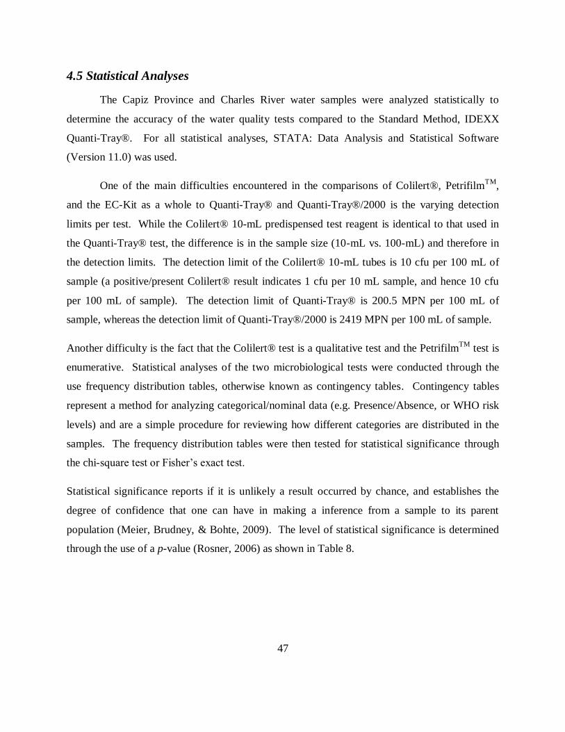
Table 8: Guidelines for assessing the significance of a p-value (Rosner, 2006). ........................ 48
Table 9: Frequency Distribution Table of Colilert® and Quanti-Tray® for E.coli Contamination
for Capiz Province .................................................................................................................... 51
Table 10: Frequency Distribution Table of PetrifilmTM
and Quanti-Tray® for E.coli
Contamination for Capiz Province ............................................................................................. 51
Table 11: Frequency Distribution Table of Colilert® and Quanti-Tray®/2000 for E.coli
Contamination of Charles River Water ...................................................................................... 52
Table 12: Frequency Distribution Table of PetrifilmTM
and Quanti-Tray® for E.coli
Contamination of Charles River Water ...................................................................................... 52
Table 13: Frequency Distribution Table of EC-Kit and Quanti-Tray® for E.coli Contamination
of Capiz Province ...................................................................................................................... 54
Table 14: 3x3 Frequency Distribution Table of EC-Kit and Quanti-Tray® for E.coli
Contamination of Charles River Water ...................................................................................... 54
10
Table 15: Error and Proportional Reduction in Error for Unimproved and Improved Water
Sources ..................................................................................................................................... 57
Table 16: Calculations for Error for Colilert® or PetrifilmTM
.................................................... 57
Table 17: Calculations for Error for EC-Kit (exact match) ......................................................... 58
Table 18: Calculations for Error for EC-Kit ............................................................................... 58
Table 19: Distribution of the 521 Drinking Water Samples Collected in Capiz Province ........... 59
Table 20: Mean Quanti-Tray® MPN E.coli Levels for Capiz Province ...................................... 60
Table 21: Mean PetrifilmTM
E.coli Counts for Capiz Province ................................................... 60
Table 22: Mean Quanti-Tray® MPN E.coli per Water Source Level for Capiz Province ........... 61
Table 23: : Mean PetrifilmTM
E.coli Count per Water Source Level for Capiz Province ............. 61
11
List of Figures
Figure 1: Map of the Philippines (Central Intelligence Agency, 2010). ...................................... 16
Figure 2: Municipalities of Capiz Province (Capiz Provincial Health Office). ........................... 20
Figure 3: Comparison between membrane filter and ColiPlate methods for enumerating E.coli in
natural water samples (Lifshitz & Joshi, 1997). ......................................................................... 26
Figure 4: Comparisons of PetrifilmTM
to three standard methods (Vail, Morgan, Merino,
Gonzales, Miller, & Ram, 2003). ............................................................................................... 28
Figure 5: Difference between typical colony counts and confirmed colony counts obtained on
mFC agar and PetrifilmTM
EC plates (Schraft & Watterworth, 2005). ........................................ 29
Figure 6: Flow diagram representing sampling/testing methodology. ........................................ 31
Figure 7: Example of a Labeled Water Sample .......................................................................... 33
Figure 8: Coliform Results of 10-mL Colilert® Tube Test ........................................................ 38
Figure 9: E.coli Results of 10-mL Colilert® Tube Test ............................................................. 38
Figure 10: Sample Total Coliform Count Plate (3M, 2001). Circles 1 and 2 are associated with
colonies with gas bubbles, circle 3 is not associated with a colony. ........................................... 41
Figure 11: Various Bubble Patterns for Gas Producing Colonies (3M, 2001). ............................ 41
Figure 12: System for Counting Coliform Colonies on PetrifilmTM
............................................ 42
Figure 13: Garmin® eTrex® GPS ............................................................................................. 46
Figure 14: Quanti-Tray® and PetrifilmTM
Water Quality Results for E.coli for Capiz Province
and Charles River Water for Different Risk Levels .................................................................... 53
Figure 15: Quanti-Tray and Petrifilm Water Quality Results for Capiz Province and Charles
River ......................................................................................................................................... 55
12
Figure 16: Water Quality Map of 160 Samples Collected in Capiz Province, Philippines .......... 62
Figure 17: Detailed Water Quality Map Results Within a Data Point ......................................... 63

13
List of Abbreviations
3M Minnesota Mining and Manufacturing Company
APHA American Public Health Association
AWWA American Water Works Association
BCIG 5-bromo-4-chloro-3-indolyl ß-D-glucuronide
cfu colony forming units
CP ColiPlate
DPH Director of Public Health
E.coli Escherichia coli
EC Escherichia coli
GPS Global positioning system
km kilometers
Lambda (λ) Proportional reduction in error
MF Membrane Filtration
MIT Massachusetts Institute of Technology
mL milliliters
MPN Most probable number
NGO Non-governmental organization
NSCB National Statistical Coordination Board
P/A Presence/absence
PHO Provincial Health Office
PNSDW Philippines National Standards for Drinking Water
SI Sanitary Inspector
TC Total coliform
TM Trademark
TNTC Too numerous to count
UN United Nations
UNICEF United Nations Children's Fund
UV Ultraviolet
WEF Water Environment Federation
WHO World Health Organization
14
CHAPTER 1: INTRODUCTION
1.1 Background
Water is a basic human need for health and survival. The United Nations (U.N.)
describes water as “indispensable for leading a life of human dignity” and “a prerequisite for the
realization of other human rights.” This right to water “entitles everyone to sufficient, safe,
acceptable, physically accessible, and affordable water for personal and domestic uses” (United
Nations, 2009). Still, thirteen percent of the world’s population, or 884 million people, lack
access to an improved drinking water source (WHO/UNICEF, 2010). Every year, at least 1.8
million people die from diarrheal diseases related to unsafe water, sanitation, and hygiene.
Furthermore, the majority is children under the age of five years old (WHO/UNICEF, 2010).
In response, the U.N. has developed the Millennium Development Goal 7 Target 3 aimed
to halve the proportion of people without sustainable access to adequate water and sanitation by
the year 2015 (United Nations, 2000). The indicators used for these numbers include the
proportion of the population that uses an improved drinking water source, and the proportion that
uses an improved sanitation facility (United Nations, 2000). The ideal solution to the problem of
unsafe water and subsequent disease is to provide reliable access to a safe drinking water supply.
According to the U.N., access to drinking water means that the source is less than one kilometer
away from its place of use, and that it is possible to reliably obtain at least 20 liters of water per
member of a household per day. The U.N. also defines safe drinking water as water with
microbial, chemical, and physical characteristics that meet World Health Organization (WHO)
guidelines or national standards on drinking water quality (United Nations, 2000).
This raises the important issue of the performance of water quality testing in order to
determine the safety of drinking water. Yet, the assessment of safe drinking water by means of
microbiological indicator testing is frequently expensive, particularly in developing countries.
This project aims to verify an inexpensive and simple water quality assessment tool, the
Escherichia coli-Kit (EC-Kit) Portable Microbiology Laboratory. Additionally, this project will
be selectively testing the water quality in Capiz Province, for the purposes of determining the
locations of unsafe drinking water supplies, so that corrective action may be taken.
15
1.2 Scope of Current Work
The current study has the following objectives:
1. To verify the field method EC-Kit under different water source conditions by comparing
it to a laboratory standard method (IDEXX Quanti-Tray®). The results of this work are
found in Chapters 4, 5, 6 and 7.
2. To conduct a detailed, in-depth controlled experiment of Charles River Water from
Cambridge, Massachusetts with multiple sample dilutions, duplicates, and blanks. The
results of this work are in Chapters 4 and 5.
3. To determine the improvement in making predictions of drinking water quality compared
to simply knowing the United Nations infrastructures designation of improved versus
unimproved water sources. The results of this work are found in Chapter 6.
4. To determine the water quality and risk level for drinking water sources according to
Escherichia coli and total coliform tests in Capiz Province for different locations and
source types. The results of this work are found in Chapters 3, 4, and 5.
5. To create a map of the water quality results from EC-Kit and Quanti-Tray®. The results
of this work are found in Chapter 6.
1.3 Overview of the Philippines
The Philippines is an archipelago composed of over 7,000 islands and is located in
Southeast Asia, between the Philippine Sea, Celebes Sea and the South China Sea. It is a
mountainous country with low-lying reaches along the coastline. The Philippines have a total
land area of approximately 300,000 km2 and an extensive coastline of over 36,000 km. There is a
tropical marine climate and two monsoon seasons: the dry, northeast monsoon from November
to April, and the wet, southwest monsoon from May to October. The country is usually subject to
15 typhoons per year and five to six cyclones, which impacts both water and land resources
(Central Intelligence Agency, 2010).
16
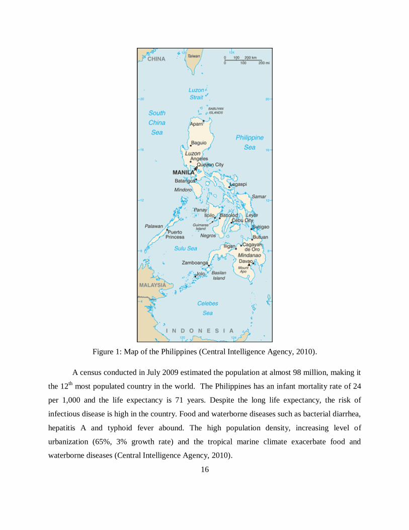
Figure 1: Map of the Philippines (Central Intelligence Agency, 2010).
A census conducted in July 2009 estimated the population at almost 98 million, making it
the 12th most populated country in the world. The Philippines has an infant mortality rate of 24
per 1,000 and the life expectancy is 71 years. Despite the long life expectancy, the risk of
infectious disease is high in the country. Food and waterborne diseases such as bacterial diarrhea,
hepatitis A and typhoid fever abound. The high population density, increasing level of
urbanization (65%, 3% growth rate) and the tropical marine climate exacerbate food and
waterborne diseases (Central Intelligence Agency, 2010).
17
The country is populated by a variety of ethnic groups, including Tagalog, Cebuano,
Llocano, Bisaya/Binisaya, Hiligaynon Llonggo, Bikal, Waray and others; in total there are over
one hundred groups (The Official Government Portal of the Republic of the Philippines, 2010).
The vast majority are Christian, with 91.5% estimated by the 2000 census (81% Roman
Catholic). The Philippines is a Democratic Republic and is divided into three geographic areas -
Luzon, Visayas, and Mindanao. There are a total of 81 provinces, 136 cities, 1,494 municipalities
and 41,995 barangays (a geographical area within a city or municipality comprised of less than
1,000 inhabitants), which are the smallest organizational unit in the Philippine political system.
The capital city is Manila, which is located in Luzon. The current President, President Gloria
Macapagal-Arroyo, has been in power since 2001 and the next election is set for May 2010.
Philippines economy is primarily based on service (commerce and government), industry
and agriculture; with a rough breakdown of >50%, 30%, <20%, respectively (United States
Department of State, 2010). Arable land and permanent crops account for approximately 35% of
the total land use, and a total of 15,000 km2
is irrigated land (in 2003). The major agriculture
products are: rice, sugarcane, coconut, corn, bananas, cassavas, pineapples, mangoes, pork, eggs,
beef, and fish. Industry includes electronics assembly, garments, footwear, pharmaceuticals,
chemicals, wood products, food processing, petroleum refining, and fishing. The GDP growth
rate in 2008 was 3.8% and the GDP per capita as of 2008 has been reported by the CIA as $3300
and by the United States Department of State as $1,841 (United States Department of State,
2010). Forty-one percent of Filipinos continue to live in rural areas and 47% of rural families
continue to live below the nationally defined poverty line in 2000, compared with 20% of urban
families (World Bank, 2006).
1.4 Water Use in the Philippines
The total renewable water resources in the Philippines in 1999 were estimated to be 479
km3 (Central Intelligence Agency, 2010). With freshwater withdrawals in 2000 estimated at
approximately 29 km3 per year; with a breakdown of 17%, 9% and 74% for domestic, industrial
and agricultural uses, respectively. Agriculture is a significant draw on the freshwater resources.
Approximately 5% (15,500 km2 / 300,000 km
2) of land area in the Philippines was irrigated in
2003. The use of irrigation is increasing, with the threats of climate change and El Niño causing
18
droughts and below average rainfall in certain areas in recent years. In fact, the President has
recently called for early completion of a major national irrigation project in light of these facts
(The Official Government Portal of the Republic of the Philippines, 2010). Thus, while the
country overall remains one of water abundance, the uneven spatial and temporal distribution are
key factors impacting emerging water use trends in the country.
1.5 Drinking Water Regulations in the Philippines
Chapter II (Water Supply), Section 9 of the Code on Sanitation of the Philippines states
that “Standards for drinking water and their microbiological and chemical examinations, together
with the evaluation of results, shall conform to the criteria set by the National Drinking Water
Standards” (The Republic of the Philippines Department of Health, 1976). In 2007, the
Philippines Department of Health formulated standards for drinking water, aiming to minimize
risk and therefore prevent health repercussions from exposure to impurities in water. The
standards set in the Philippines National Standards for Drinking Water (PNSDW) 2007 are based
on guidelines or criteria recommended by international institutions like the WHO. The
Philippines National Standards for Drinking Water (PNSDW 2007) addressed water quality
issues by setting more comprehensive parameters, advocating a surveillance system, and
prioritizing the parameters that need to be monitored (The Republic of Philippines Department of
Health, 2007).
The WHO Joint Monitoring Programme for Water Supply and Sanitation has been
assembling statistics on drinking water and sanitation coverage since 1990. Since 2000, the Joint
Monitoring Programme has classified water sources as “improved” or “unimproved”
(WHO/UNICEF Joint Monitoring Programme for Water Supply and Sanitation, 2005). The
classification of “improved” and “unimproved” water technologies are shown in Table 1.
19
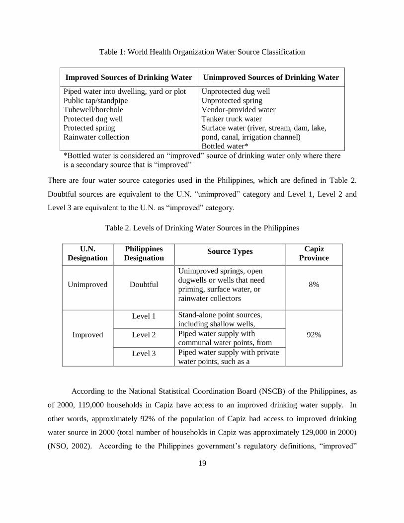
Table 1: World Health Organization Water Source Classification
Improved Sources of Drinking Water Unimproved Sources of Drinking Water
Piped water into dwelling, yard or plot
Public tap/standpipe
Tubewell/borehole
Protected dug well
Protected spring
Rainwater collection
Unprotected dug well
Unprotected spring
Vendor-provided water
Tanker truck water
Surface water (river, stream, dam, lake,
pond, canal, irrigation channel)
Bottled water*
*Bottled water is considered an “improved” source of drinking water only where there
is a secondary source that is “improved”
There are four water source categories used in the Philippines, which are defined in Table 2.
Doubtful sources are equivalent to the U.N. “unimproved” category and Level 1, Level 2 and
Level 3 are equivalent to the U.N. as “improved” category.
Table 2. Levels of Drinking Water Sources in the Philippines
U.N.
Designation
Philippines
Designation Source Types Capiz
Province
Unimproved Doubtful
Unimproved springs, open
dugwells or wells that need
priming, surface water, or
rainwater collectors
8%
Improved
Level 1 Stand-alone point sources,
including shallow wells,
tubewells with handpumps 92% Level 2 Piped water supply with
communal water points, from
boreholes, tubewells Level 3 Piped water supply with private
water points, such as a
household connection
According to the National Statistical Coordination Board (NSCB) of the Philippines, as
of 2000, 119,000 households in Capiz have access to an improved drinking water supply. In
other words, approximately 92% of the population of Capiz had access to improved drinking
water source in 2000 (total number of households in Capiz was approximately 129,000 in 2000)
(NSO, 2002). According to the Philippines government’s regulatory definitions, “improved”
20
water sources include three levels: Level 1 consists of point sources, Level 2 consists of
communal faucet systems, and Level 3 consists of piping systems with individual household
connections. The unimproved water sources, also called “doubtful sources,” consist of open dug
wells, unimproved springs, rainwater and surface water sources.
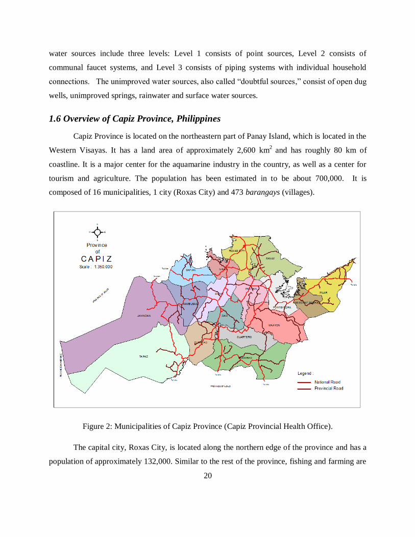
1.6 Overview of Capiz Province, Philippines
Capiz Province is located on the northeastern part of Panay Island, which is located in the
Western Visayas. It has a land area of approximately 2,600 km2
and has roughly 80 km of
coastline. It is a major center for the aquamarine industry in the country, as well as a center for
tourism and agriculture. The population has been estimated in to be about 700,000. It is
composed of 16 municipalities, 1 city (Roxas City) and 473 barangays (villages).
Figure 2: Municipalities of Capiz Province (Capiz Provincial Health Office).
The capital city, Roxas City, is located along the northern edge of the province and has a
population of approximately 132,000. Similar to the rest of the province, fishing and farming are
21
the major economic activities; which together use just over 50% of the total land area. The
dominant agricultural crop is rice, with over 38 km2 of land used for rice fields. Other major
crops include coconuts, bananas, watermelons, leafy vegetables, mungo, various citrus crops and
mango. Both freshwater and brackish water aquaculture is common, as the swampy coastline
lends itself well to fishpond development. In fact, over 840 km2 are used for brackish fishpond
development. Marine fishing and livestock production are also major industries in the area. As
the only urban area in the province, Roxas City is a center of trade and commerce, and as a result
is becoming increasingly industrialized and commercialized.
Until 2009, Capiz had never performed any drinking water quality testing on the various
drinking water sources (wells, springs, surface water and piped supplies) used throughout the
province, with the exception of those performed in the Roxas City municipal water treatment
plant. The Provincial Health Office (PHO) of Capiz Province decided to undertake the water
quality testing in the province. The main PHO participants in this project included Dr. Jarvis
Punsalan, MD, Director of Public Health (DPH) head of the Capiz PHO; Jane delos Reyes,
Engineer, coordinator of the water quality testing program; Leo Biclar, medical technician
responsible for processing and interpreting the Quanti-Tray® tests; and Sanitary Inspectors (SI’s)
at the provincial and municipal levels who were in charge of collecting the water samples and
processing and interpreting one of the microbiological tests used.
During Fall 2008, Dr. Jarvis Punsalan received funding from the European Commission,
the Philippines’ government’s Department of Health, and United Nations Children’s Fund
(UNICEF) to set up a water quality testing laboratory at Roxas Memorial Hospital, in Roxas
City, which would test for microbiological contamination. He contacted Susan Murcott, Senior
Lecturer at the Massachusetts Institute of Technology (MIT), for advice on the types of
microbiological drinking water quality tests to conduct, and she recommended two types of tests:
Quanti-Tray® and EC-Kit. Quanti-Tray® is an enzyme-substrate coliform test (Standard
Methods 9223) based on Most Probable Number (MPN) and has been approved in more than 35
countries worldwide. The EC-Kit is a new portable microbiological testing kit comprised of two,
easy-to-use tests: the 10-mL Presence/Absence (P/A) Colilert® and the enumerative test: 3MTM
PetrifilmTM
. The innovation of combining these two tests in the EC-Kit was the idea of Dr.
22
Robert Metcalf, one of the original founders of solar cookers international and Professor of
Microbiology at California State University at Sacramento. He introduced this method to Susan
Murcott, in Kenya in 2005. She in turn developed the EC-Kit, which included all the items,
including a waist belt incubator, and other materials needed in order to perform and interpret the
tests. Susan Murcott introduced the technology to the Non-Governmental Organization (NGO)
“A Single Drop”, and introduced the director of that NGO to Robert Metcalf, after which they
brought the technology to the Philippines.
During 2009, Capiz’s PHO purchased EC-Kits and Quanti-Tray® tests. An incubator,
ultraviolet (UV) light and Quanti-Tray® sealer were also purchased in order to conduct the
Quanti-Tray® tests. In May 2009, “A Single Drop” trained the Capiz PHO staff, municipal
health officers and SI’s on how to sample water sources, use the EC-Kit and interpret the sample
results. The Quanti-Tray® equipments finally arrived in November 2009, and as part of that
purchase, the laboratory staff of the PHO’s Roxas City office received training for the suppliers
in the set up and use of the Quanti-Tray® system. From October to December 2009, in
collaboration with the MIT team, the PHO developed a water quality assessment survey designed
to test 1,000 different water supplies from all 16 municipalities and Roxas City, which took place
from December 2009 to March 2010. This would be the first-ever comprehensive drinking water
quality testing in the province.
23
CHAPTER 2: LITERATURE REVIEW
2.1 Indicator Microorganisms
There are a large variety of bacteria, parasites, and viruses that can cause illness when
humans ingest them in drinking water. However, testing drinking water for all possible disease-
causing agents would be difficult, time-consuming, and expensive. Instead, monitoring drinking
water quality relies on the detection of indicator organisms. According to the WHO (World
Health Organization, 2006), ideal indicator organisms should:
1. be universally present in feces of humans and animals in large numbers;
2. not multiply in natural waters;
3. persist in water in a similar manner to fecal pathogens;
4. be present in higher numbers than fecal pathogens;
5. respond to treatment processes in a similar fashion to fecal pathogens; and
6. be readily detected by simple, inexpensive methods.
While there is no perfect indicator organism, Escherichia coli is considered the most reliable
indicator of fecal contamination (Doyle & Erickson, 2006). E. coli and thermotolerant coliforms
are a subset of the total coliform group. Total coliform bacteria are defined as aerobic and
facultatively anaerobic, gram-negative, non-spore forming, rod-shaped bacteria that produce gas
upon lactose fermentation in prescribed culture media after 24 hours of incubation at 35°C
(World Health Organization, 2006). Total coliform counts are used to monitor water treatment,
but total coliforms include both fecal and environmental species. Therefore, to avoid the
limitations of total coliforms, E. coli and thermotolerant coliforms are widely accepted as good
indicators for fecal contamination.
2.2 Overview of Microbial Assay Methods
For analyzing drinking water quality, particularly in routine public water supply
examination, the object is to determine the efficiency of treatment plant operation, the integrity
of the distribution system, and to screen for the presence of fecal contamination (APHA, WEF,
AWWA, 2005). The four Standard Methods (SM) most commonly used to identify coliforms in
24
water include multiple-tube fermentation (SM#9221A), presence/absence (SM #9221D),
membrane filtration (SM #9222), and enzyme substrate (chromogenic) (SM #9223).
In the multiple-tube fermentation test, multiple tubes are used in the fermentation, and the
Most Probable Number (MPN) of organisms present is reported. When utilizing multiple-tube
fermentation, the precision of each test depends on the number of tubes used.
The presence-absence (P-A) test for coliforms is a modified, simpler version of the
multiple-tube fermentation test. The P-A test operates under the theory that no coliforms should
be present in 100 mL of a drinking water sample, and so it is possible to conduct a test using one
test volume. The P-A test is intended for use on routine samples collected from distribution
systems or water treatment plants. However, in the event of a positive result for coliforms
(presence), it is advisable to determine coliform densities in repeat samples and/or other tests
(APHA, WEF, AWWA, 2005).
The membrane filter (MF) technique, as described in Standard Methods for Examination
of Water and Wastewater, 21st edition, is routinely used worldwide to quantify density of
coliforms and E. coli in water and wastewater (Lifshitz & Joshi, 1997). The MF technique is
highly reproducible, can test relatively large sample volumes, and yields numerical results faster
than multiple-tube fermentation. However, the MF technique has limitations in testing waters
with high turbidity or large numbers of noncoliform bacteria because the presence of algae,
particulates, or other interfering material may not permit testing of sufficient sample volume to
yield significant results (APHA, WEF, AWWA, 2005).
The enzyme substrate test is recommended for the analysis of drinking and source water
samples (APHA, WEF, AWWA, 2005), but it is emphasized for laboratories using this text to
conduct parallel quantitative testing ( including seasonal variations with one of the standard
coliform tests to assess the effectiveness of the test for the specific water type, particularly when
testing source waters. The enzyme substrate test is not recommended for presumptive coliform
cultures or membrane filter colonies because it may lead to false positives.
2.3 Quanti-Tray® and Quanti-Tray®/2000
The IDEXX Quanti-Tray® and Quanti-Tray®/2000 are enzyme substrate coliform tests
that utilize semi-automated quantification methods based on the Standard Methods Most
25
Probable Number (MPN) model, which provides the MPN of colony forming units (cfu). The
tests have been approved in over 35 countries worldwide (IDEXX, 2009). The trays provide
bacterial counts of up to 200.5 MPN per 100 mL of sample (or 2419 MPN per 100 mL of sample
for Quanti-Tray®/2000).
The Quanti-Tray® is easy, rapid, and accurate. There is no colony counting required, no
dilutions needed for counts up to 2,419, and no media preparation. The Quanti-Tray® detects
down to 1 cfu per 100 mL of sample, and has better 95% confidence limits than multiple tube
fermentation or membrane filtration (Thermalindo, 2007). However, the cost of equipment and
supplies for Quanti-Tray® is expensive, particularly in developing countries.
2.4 EC-Kit
The EC-Kit is a simple, inexpensive field test kit that contains two complementary tests
for E. coli: the Colilert® 10 mL presence/absence test and 3M™’s PetrifilmTM
test. The kit also
includes sterile sampling bags, a sterile 3.5-mL pipette, an ultraviolet light with batteries,
cardboard squares, rubber bands, and a waist-belt incubator. The 10 mL pre-dispensed Colilert®
test indicates presence/absence of coliform bacteria, and specifically whether E. coli is present in
the 10 mL of water tested. The PetrifilmTM
test provides a quantitative count of total coliform
bacteria and E. coli present in the volume sampled.
2.5 Studies on Colilert® Reagent
Olson et al. compared Colilert® and ColiQuik1 systems in presence-absence format
against the Standard Methods Membrane Filtration (MF) technique for total coliform detection,
and observed a greater than 94.8% agreement in two-way comparisons (Colilert® with MF,
ColiQuik with MF) (Olson, Clark, Milner, Stewart, & Wolfe, 1991). When laboratory and field
inoculation methods were compared for Colilert®, more than 98% agreement was obtained. Due
to the presence of false negatives in the study, the researchers indicated the importance of using
field data and not spiked water samples in future studies.
1 ColiQuik is suitable for testing salt water, chemically treated water and wash from meat, fish and vegetable
preparation. USA Patent No. 6051394. http://www.b2ptesting.com.au/Coliquik%20Pack%20Insert_LATEST.pdf
(B2P Testing, Auckland, New Zealand)
26
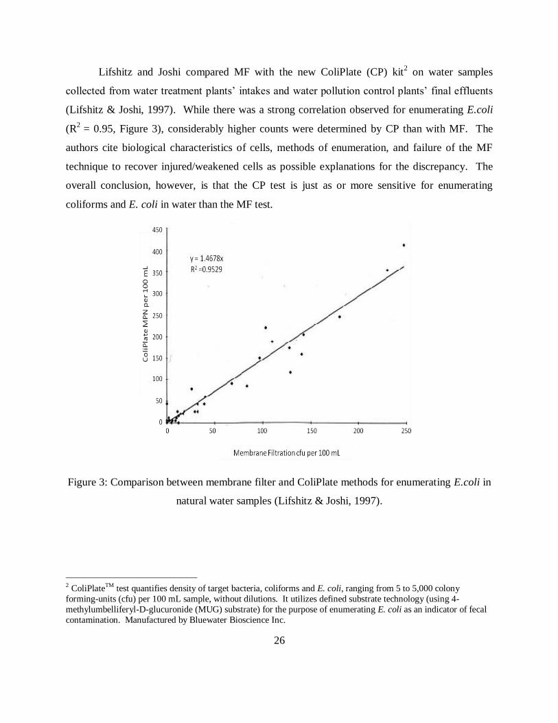
Lifshitz and Joshi compared MF with the new ColiPlate (CP) kit2 on water samples
collected from water treatment plants’ intakes and water pollution control plants’ final effluents
(Lifshitz & Joshi, 1997). While there was a strong correlation observed for enumerating E.coli
(R2
= 0.95, Figure 3), considerably higher counts were determined by CP than with MF. The
authors cite biological characteristics of cells, methods of enumeration, and failure of the MF
technique to recover injured/weakened cells as possible explanations for the discrepancy. The
overall conclusion, however, is that the CP test is just as or more sensitive for enumerating
coliforms and E. coli in water than the MF test.
Figure 3: Comparison between membrane filter and ColiPlate methods for enumerating E.coli in
natural water samples (Lifshitz & Joshi, 1997).
2 ColiPlateTM test quantifies density of target bacteria, coliforms and E. coli, ranging from 5 to 5,000 colony
forming-units (cfu) per 100 mL sample, without dilutions. It utilizes defined substrate technology (using 4-
methylumbelliferyl-D-glucuronide (MUG) substrate) for the purpose of enumerating E. coli as an indicator of fecal
contamination. Manufactured by Bluewater Bioscience Inc.
27
Fricker et al. compared the newer form of Colilert®, Colilert®-18, to MF (Fricker,
Illingworth, & Fricker, 1997). Colilert®-18 provides results within 18 hours instead of the
traditional 24-hour Colilert® test. Their study showed that there was no significant difference
between the two Colilert® and Colilert®-18 forms of the product. Colilert®-18 showed similar
results to membrane filtration. Therefore, both formulations of the Colilert® reagent, Colilert®
and Colilert®-18, were suitable alternatives to the membrane filtration method for
bacteriological monitoring of drinking water quality (Fricker, Illingworth, & Fricker, 1997).
Years later, in 2003, Chao et al. conducted an edifying study on the accuracy of
Colilert®-18 as a test for coliforms and E. coli. It was found that Colilert®-18 produced a low
false-negative rate, and would serve well as a technique for monitoring subtropical freshwaters.
The authors point out that for some countries, total coliform number still serves as the sole
indicator microorganism, and Colilert®-18 tends to give higher total coliform counts than the
traditional methods, such as membrane filtration. Otherwise, it was also concluded that
Colilert®-18 is satisfactory for rapid screening for fecal contamination in subtropical freshwater
(Chao, Chao, & Chao, 2004).
From these studies on Colilert® reagent and given what is known about Quanti-Tray®, is
clear that Colilert® is comparable to Colilert®-18, and that both are suitable alternatives to the
membrane filtration Standard Method. Colilert®-18 produces a low false negative rate, and may
even be more sensitive for enumerating coliforms. Thus, Quanti-Tray® and Colilert® (or
Colilert®-18) are apt for use as the standard water quality test to which the EC-Kit will be
compared for verification.
2.6 Studies on 3M PetrifilmTM
In a study conducted by Vail et al., PetrifilmTM
total coliform count plates (Manufactured
by 3MTM
, Minneapolis, Minnesota), previously used for enumerating E. coli in food, were tested
for monitoring E. coli in environmental waters (Vail, Morgan, Merino, Gonzales, Miller, & Ram,
2003). The study compared enumeration of E. coli in water samples using PetrifilmTM
to three
commonly used commercially available tests: membrane filtration using mColiBlue media,
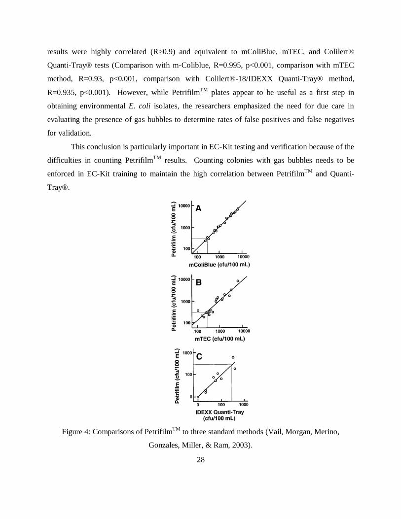
mTEC media, and Colilert® Quanti-Tray® (Figure 4). The data was normalized to 100 mL and
transformed with log[cfu/100 +10] prior to linear regression. It was concluded that PetrifilmTM
28
results were highly correlated (R>0.9) and equivalent to mColiBlue, mTEC, and Colilert®
Quanti-Tray® tests (Comparison with m-Coliblue, R=0.995, p<0.001, comparison with mTEC
method, R=0.93, p<0.001, comparison with Colilert®-18/IDEXX Quanti-Tray® method,
R=0.935, p<0.001). However, while PetrifilmTM
plates appear to be useful as a first step in
obtaining environmental E. coli isolates, the researchers emphasized the need for due care in
evaluating the presence of gas bubbles to determine rates of false positives and false negatives
for validation.
This conclusion is particularly important in EC-Kit testing and verification because of the
difficulties in counting PetrifilmTM
results. Counting colonies with gas bubbles needs to be
enforced in EC-Kit training to maintain the high correlation between PetrifilmTM
and Quanti-
Tray®.
Figure 4: Comparisons of PetrifilmTM
to three standard methods (Vail, Morgan, Merino,
Gonzales, Miller, & Ram, 2003).

29
Schraft & Watterworth (2005) compared PetrifilmTM
with standard plating procedures
(mFC-agar plates) on naturally contaminated water samples for enumeration of heterotrophs,
fecal coliforms, and E. coli in water (Schraft & Watterworth, 2005). On mFC agar, counts for
typical colonies were 2 log10 cfu higher than the actual confirmed counts (confirmed via
biochemical identification using Standard Procedures for Water Analysis, sections 9221B,
9221E, 9225A), whereas PetrifilmTM
EC plates were almost identical to confirmed colony counts
for both fecal coliforms and E.coli (Figure 5). Thus, it was found that PetrifilmTM
plates seemed
more selective for fecal coliforms and E. coli.
Figure 5: Difference between typical colony counts and confirmed colony counts obtained on
mFC agar and PetrifilmTM
EC plates (Schraft & Watterworth, 2005).
This study is one of the few studies evaluating the use of PetriflmTM
as a test for water quality.
PetrifilmTM
is more selective for fecal coliforms and E.coli, meaning that it is a better “match” to
the confirmed counts than the standard plating procedure using mFC-agar. However, there have
been no studies evaluating the use of PetrifilmTM
as a field test to be used outside of the
laboratory, as this study aims to do.
30
CHAPTER 3: RESEARCH AND SAMPLING DESIGN
3.1 Overview of Research and Sampling Design
Capiz Provincial Health Officer Dr. Jarvis Punsalan (MD, MPH), and Sanitary Inspector
Jane Delos Reyes, commenced the 1,000 test set program covering 16 municipalities and Roxas
City in December 2009. The author travelled to and worked in Capiz for approximately 22
working days, beginning on January 7, 2010, together with three other Master of Engineering
teammates and their project advisor. The study design was prepared by Punsalan and Reyes, in
collaboration with Susan Murcott of the Massachusetts Institute of Technology (MIT), Tom
Mahin of the Massachusetts Department of Environmental Protection, and our four-person
Masters of Engineering student team. The overarching objective for all collaborators was to (i)
Determine, for the first time, the water quality in the 16 municipalities and Roxas City, (ii)
Compare two different test methods: Quanti-Tray® and EC-Kit to determine if the EC-Kit is a
reliable field test method for local application beyond this study, (iii) Evaluate the chlorine
residual levels in Roxas City to determine if they met the PNSDW regulatory standards and (iv)
Based on sanitary inspector and stakeholder interviews and community assessments, make
recommendations on how to increase the safety of drinking water in Capiz Province.
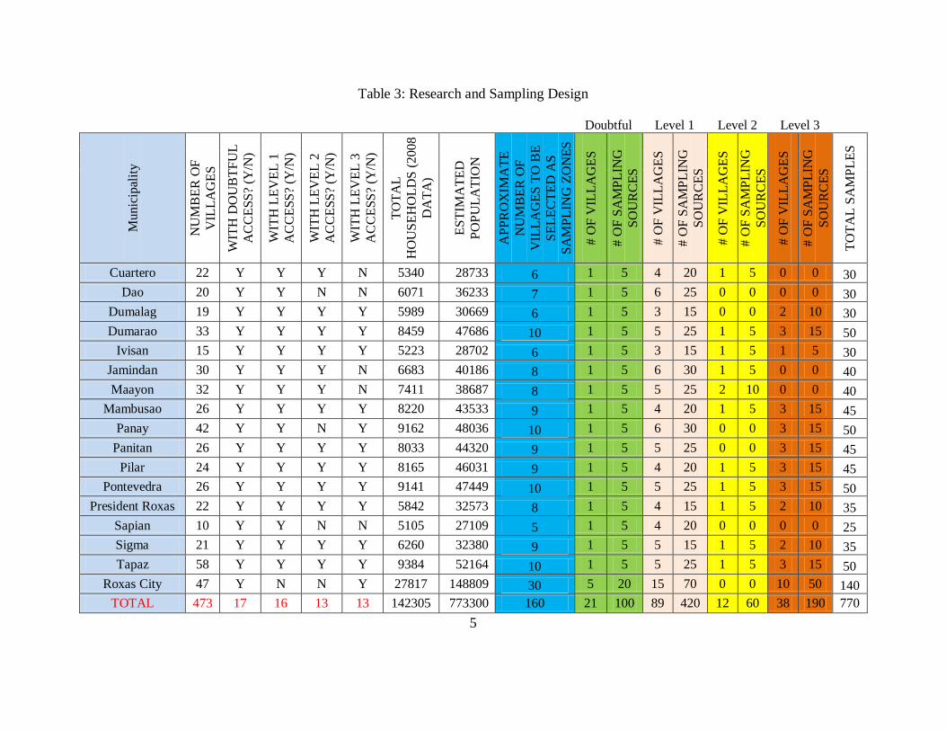
The number of villages or sampling zones for each municipality was computed based on
the following criteria (Table 3): a ratio of 1 sampling zone for every 5,000 population (e.g. a
municipality with a population of 30,000 would have 6 sampling zones selected). Zones were
distributed according to ratio of water sources accessed by the residents of the particular
municipality.
Water samples were randomly selected: the names of qualified villages or zones per town
were put in a box and drawn randomly with 25% additional names drawn as reserve in case of
inaccessibility of those initially selected. Water source selection was based on accessibility and
their use by at least ten nearby households in the sampling zone:
For each selected zone having doubtful sources, five of these sources were randomly
selected and tested.
31
For each village randomly selected for Level 1 supply testing, five Level 1 water sources
were randomly selected for testing.
For each village randomly selected for Level 2 supply testing, one reservoir was
randomly selected and five of its outlets were tested. Water sources tested were the
reservoir outlets. A maximum of five outlets per reservoir were tested.
For each village randomly selected for Level 3 supply testing, five households accessing
water from these sources were randomly selected and tested per zone. Water sources
tested were every tenth household within the zone until the needed number of samples
(five) was attained.
The only exception to the aforementioned study design was the Level 3 water supply for Roxas
City. Since all of Roxas City has a piped, chlorinated water supply, this was tested separately
using chlorine residual testing instead of the costlier bacteriological testing.
5
Table 3: Research and Sampling Design
Doubtful Level 1 Level 2 Level 3
M
unic
ipal
ity
NU
MB
ER
OF
VIL
LA
GE
S
WIT
H D
OU
BT
FU
L
AC
CE
SS
? (Y
/N)
WIT
H L
EV
EL
1
AC
CE
SS
? (Y
/N)
WIT
H L
EV
EL
2
AC
CE
SS
? (Y
/N)
WIT
H L
EV
EL
3
AC
CE
SS
? (Y
/N)
TO
TA
L
HO
US
EH
OL
DS
(2008
DA
TA
)
ES
TIM
AT
ED
PO
PU
LA
TIO
N
AP
PR
OX
IMA
TE
NU
MB
ER
OF
VIL
LA
GE
S T
O B
E
SE
LE
CT
ED
AS
SA
MP
LIN
G Z
ON
ES
# O
F V
ILL
AG
ES
# O
F S
AM
PL
ING
SO
UR
CE
S
# O
F V
ILL
AG
ES
# O
F S
AM
PL
ING
SO
UR
CE
S
# O
F V
ILL
AG
ES
# O
F S
AM
PL
ING
SO
UR
CE
S
# O
F V
ILL
AG
ES
# O
F S
AM
PL
ING
SO
UR
CE
S
TO
TA
L S
AM
PL
ES
Cuartero 22 Y Y Y N 5340 28733 6 1 5 4 20 1 5 0 0 30
Dao 20 Y Y N N 6071 36233 7 1 5 6 25 0 0 0 0 30
Dumalag 19 Y Y Y Y 5989 30669 6 1 5 3 15 0 0 2 10 30
Dumarao 33 Y Y Y Y 8459 47686 10 1 5 5 25 1 5 3 15 50
Ivisan 15 Y Y Y Y 5223 28702 6 1 5 3 15 1 5 1 5 30
Jamindan 30 Y Y Y N 6683 40186 8 1 5 6 30 1 5 0 0 40
Maayon 32 Y Y Y N 7411 38687 8 1 5 5 25 2 10 0 0 40
Mambusao 26 Y Y Y Y 8220 43533 9 1 5 4 20 1 5 3 15 45
Panay 42 Y Y N Y 9162 48036 10 1 5 6 30 0 0 3 15 50
Panitan 26 Y Y Y Y 8033 44320 9 1 5 5 25 0 0 3 15 45
Pilar 24 Y Y Y Y 8165 46031 9 1 5 4 20 1 5 3 15 45
Pontevedra 26 Y Y Y Y 9141 47449 10 1 5 5 25 1 5 3 15 50
President Roxas 22 Y Y Y Y 5842 32573 8 1 5 4 15 1 5 2 10 35
Sapian 10 Y Y N N 5105 27109 5 1 5 4 20 0 0 0 0 25
Sigma 21 Y Y Y Y 6260 32380 9 1 5 5 15 1 5 2 10 35
Tapaz 58 Y Y Y Y 9384 52164 10 1 5 5 25 1 5 3 15 50
Roxas City 47 Y N N Y 27817 148809 30 5 20 15 70 0 0 10 50 140
TOTAL 473 17 16 13 13 142305 773300 160 21 100 89 420 12 60 38 190 770
31
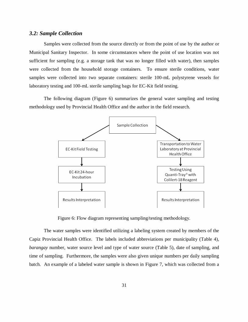
3.2: Sample Collection
Samples were collected from the source directly or from the point of use by the author or
Municipal Sanitary Inspector. In some circumstances where the point of use location was not
sufficient for sampling (e.g. a storage tank that was no longer filled with water), then samples
were collected from the household storage containers. To ensure sterile conditions, water
samples were collected into two separate containers: sterile 100-mL polystyrene vessels for
laboratory testing and 100-mL sterile sampling bags for EC-Kit field testing.
The following diagram (Figure 6) summarizes the general water sampling and testing
methodology used by Provincial Health Office and the author in the field research.
Figure 6: Flow diagram representing sampling/testing methodology.
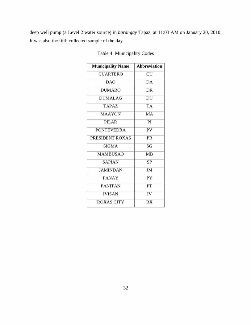
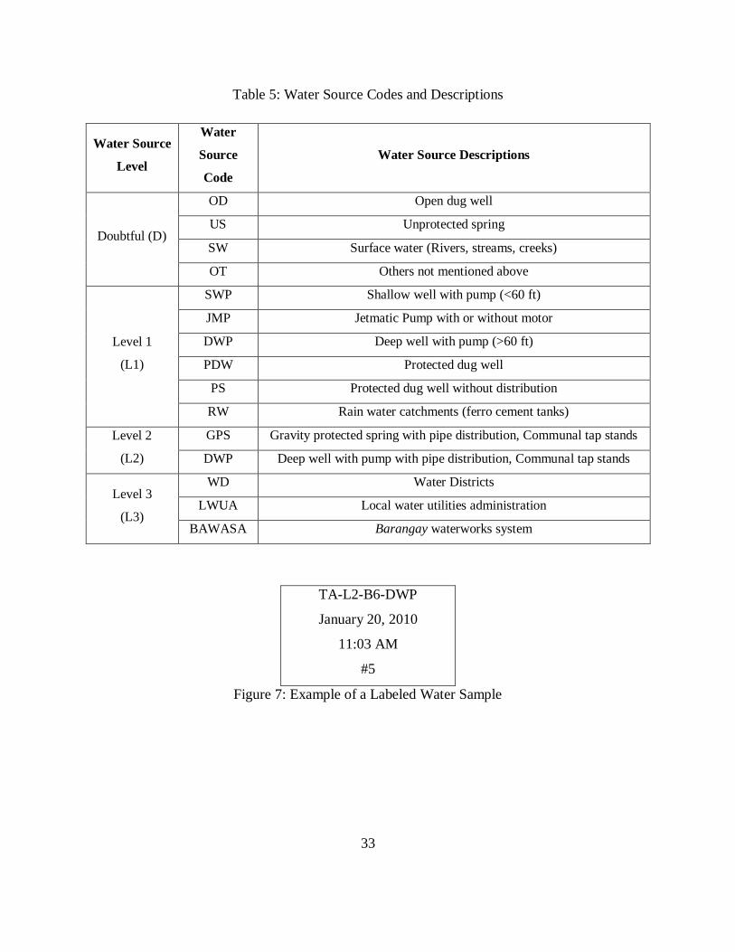
The water samples were identified utilizing a labeling system created by members of the
Capiz Provincial Health Office. The labels included abbreviations per municipality (Table 4),
barangay number, water source level and type of water source (Table 5), date of sampling, and
time of sampling. Furthermore, the samples were also given unique numbers per daily sampling
batch. An example of a labeled water sample is shown in Figure 7, which was collected from a
32
deep well pump (a Level 2 water source) in barangay Tapaz, at 11:03 AM on January 20, 2010.
It was also the fifth collected sample of the day.
Table 4: Municipality Codes
Municipality Name Abbreviation
CUARTERO CU
DAO DA
DUMARO DR
DUMALAG DU
TAPAZ TA
MAAYON MA
PILAR PI
PONTEVEDRA PV
PRESIDENT ROXAS PR
SIGMA SG
MAMBUSAO MB
SAPIAN SP
JAMINDAN JM
PANAY PY
PANITAN PT
IVISAN IV
ROXAS CITY RX
33
Table 5: Water Source Codes and Descriptions
Water Source
Level
Water
Source
Code
Water Source Descriptions
Doubtful (D)
OD Open dug well
US Unprotected spring
SW Surface water (Rivers, streams, creeks)
OT Others not mentioned above
Level 1
(L1)
SWP Shallow well with pump (<60 ft)
JMP Jetmatic Pump with or without motor
DWP Deep well with pump (>60 ft)
PDW Protected dug well
PS Protected dug well without distribution
RW Rain water catchments (ferro cement tanks)
Level 2
(L2)
GPS Gravity protected spring with pipe distribution, Communal tap stands
DWP Deep well with pump with pipe distribution, Communal tap stands
Level 3
(L3)
WD Water Districts
LWUA Local water utilities administration
BAWASA Barangay waterworks system
TA-L2-B6-DWP
January 20, 2010
11:03 AM
#5
Figure 7: Example of a Labeled Water Sample
34
CHAPTER 4: METHODOLOGY
4.1 Procedure for Quanti-Tray® Test
The Quanti-Tray® test was utilized as the standard against which the EC-Kit was
compared (see MIT teammate thesis of Trottier, 2010 for hydrogen sulfide bacteria and
Easygel® field test kit comparisons with Quanti-Tray®). After collection of 100-mL water
samples in the sterile 120-mL capacity vessels3, the samples were placed in ice chests containing
ice or ice packs and taken to the water laboratory at the Capiz Provincial Health Office. The
Provincial Health Office and MIT team used the following procedure to run the Quanti-Tray®
test:
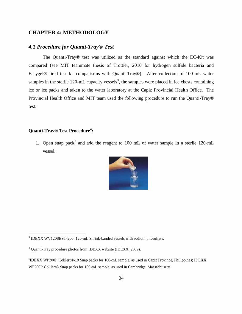
Quanti-Tray® Test Procedure4:
1. Open snap pack5 and add the reagent to 100 mL of water sample in a sterile 120-mL
vessel.
3 IDEXX WV120SBST-200: 120-mL Shrink-banded vessels with sodium thiosulfate.
4 Quanti-Tray procedure photos from IDEXX website (IDEXX, 2009).
5IDEXX WP200I: Colilert®-18 Snap packs for 100-mL sample, as used in Capiz Province, Philippines; IDEXX
WP200I: Colilert® Snap packs for 100-mL sample, as used in Cambridge, Massachusetts.
35
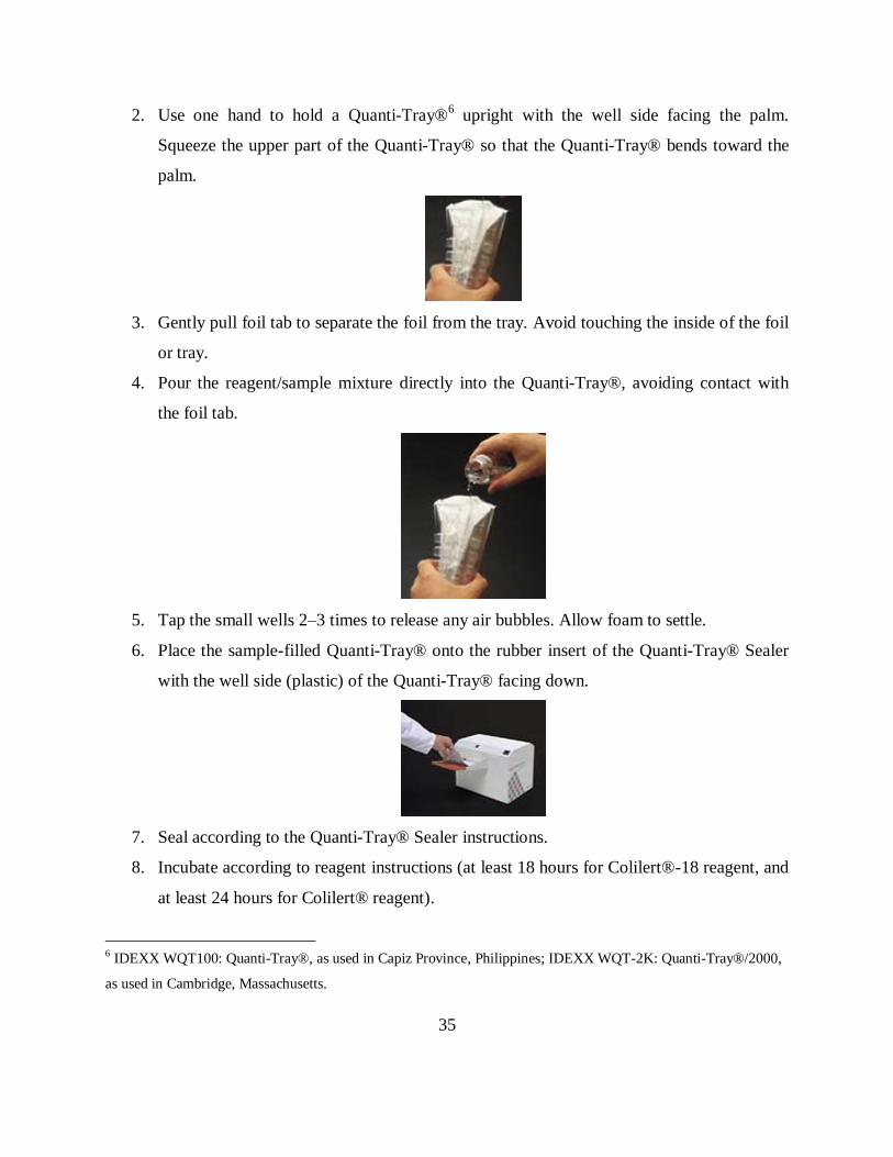
2. Use one hand to hold a Quanti-Tray®6 upright with the well side facing the palm.
Squeeze the upper part of the Quanti-Tray® so that the Quanti-Tray® bends toward the
palm.
3. Gently pull foil tab to separate the foil from the tray. Avoid touching the inside of the foil
or tray.
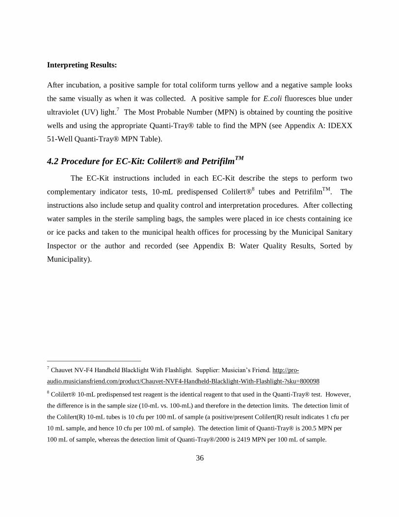
4. Pour the reagent/sample mixture directly into the Quanti-Tray®, avoiding contact with
the foil tab.
5. Tap the small wells 2–3 times to release any air bubbles. Allow foam to settle.
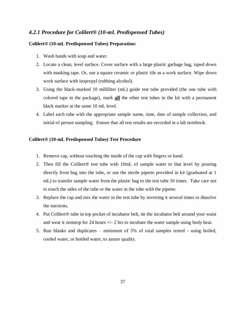
6. Place the sample-filled Quanti-Tray® onto the rubber insert of the Quanti-Tray® Sealer
with the well side (plastic) of the Quanti-Tray® facing down.
7. Seal according to the Quanti-Tray® Sealer instructions.
8. Incubate according to reagent instructions (at least 18 hours for Colilert®-18 reagent, and
at least 24 hours for Colilert® reagent).
6 IDEXX WQT100: Quanti-Tray®, as used in Capiz Province, Philippines; IDEXX WQT-2K: Quanti-Tray®/2000,
as used in Cambridge, Massachusetts.
36
Interpreting Results:
After incubation, a positive sample for total coliform turns yellow and a negative sample looks
the same visually as when it was collected. A positive sample for E.coli fluoresces blue under
ultraviolet (UV) light.7 The Most Probable Number (MPN) is obtained by counting the positive
wells and using the appropriate Quanti-Tray® table to find the MPN (see Appendix A: IDEXX
51-Well Quanti-Tray® MPN Table).
4.2 Procedure for EC-Kit: Colilert® and PetrifilmTM
The EC-Kit instructions included in each EC-Kit describe the steps to perform two
complementary indicator tests, 10-mL predispensed Colilert®8 tubes and Petrifilm
TM. The
instructions also include setup and quality control and interpretation procedures. After collecting
water samples in the sterile sampling bags, the samples were placed in ice chests containing ice
or ice packs and taken to the municipal health offices for processing by the Municipal Sanitary
Inspector or the author and recorded (see Appendix B: Water Quality Results, Sorted by
Municipality).
7 Chauvet NV-F4 Handheld Blacklight With Flashlight. Supplier: Musician’s Friend. http://pro-
audio.musiciansfriend.com/product/Chauvet-NVF4-Handheld-Blacklight-With-Flashlight-?sku=800098
8 Colilert® 10-mL predispensed test reagent is the identical reagent to that used in the Quanti-Tray® test. However,
the difference is in the sample size (10-mL vs. 100-mL) and therefore in the detection limits. The detection limit of
the Colilert(R) 10-mL tubes is 10 cfu per 100 mL of sample (a positive/present Colilert(R) result indicates 1 cfu per
10 mL sample, and hence 10 cfu per 100 mL of sample). The detection limit of Quanti-Tray® is 200.5 MPN per
100 mL of sample, whereas the detection limit of Quanti-Tray®/2000 is 2419 MPN per 100 mL of sample.
37
4.2.1 Procedure for Colilert® (10-mL Predispensed Tubes)
Colilert® (10-mL Predispensed Tubes) Preparation:
1. Wash hands with soap and water.
2. Locate a clean, level surface. Cover surface with a large plastic garbage bag, taped down
with masking tape. Or, use a square ceramic or plastic tile as a work surface. Wipe down
work surface with isopropyl (rubbing alcohol).
3. Using the black-marked 10 milliliter (mL) guide test tube provided (the one tube with
colored tape in the package), mark all the other test tubes in the kit with a permanent
black marker at the same 10 mL level.
4. Label each tube with the appropriate sample name, time, date of sample collection, and
initial of person sampling. Ensure that all test results are recorded in a lab notebook.
Colilert® (10-mL Predispensed Tubes) Test Procedure
1. Remove cap, without touching the inside of the cap with fingers or hand.
2. Then fill the Colilert® test tube with 10mL of sample water to that level by pouring
directly from bag into the tube, or use the sterile pipette provided in kit (graduated at 1
mL) to transfer sample water from the plastic bag to the test tube 10 times. Take care not
to touch the sides of the tube or the water in the tube with the pipette.
3. Replace the cap and mix the water in the test tube by inverting it several times to dissolve
the nutrients.
4. Put Colilert® tube in top pocket of incubator belt, tie the incubator belt around your waist
and wear it nonstop for 24 hours +/- 2 hrs to incubate the water sample using body heat.
5. Run blanks and duplicates – minimum of 5% of total samples tested - using boiled,
cooled water, or bottled water, to assure quality.
38
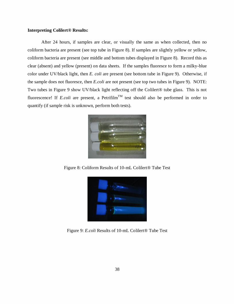
Interpreting Colilert® Results:
After 24 hours, if samples are clear, or visually the same as when collected, then no
coliform bacteria are present (see top tube in Figure 8). If samples are slightly yellow or yellow,
coliform bacteria are present (see middle and bottom tubes displayed in Figure 8). Record this as
clear (absent) and yellow (present) on data sheets. If the samples fluoresce to form a milky-blue
color under UV/black light, then E. coli are present (see bottom tube in Figure 9). Otherwise, if
the sample does not fluoresce, then E.coli are not present (see top two tubes in Figure 9). NOTE:
Two tubes in Figure 9 show UV/black light reflecting off the Colilert® tube glass. This is not
fluorescence! If E.coli are present, a PetrifilmTM
test should also be performed in order to
quantify (if sample risk is unknown, perform both tests).
Figure 8: Coliform Results of 10-mL Colilert® Tube Test
Figure 9: E.coli Results of 10-mL Colilert® Tube Test
39
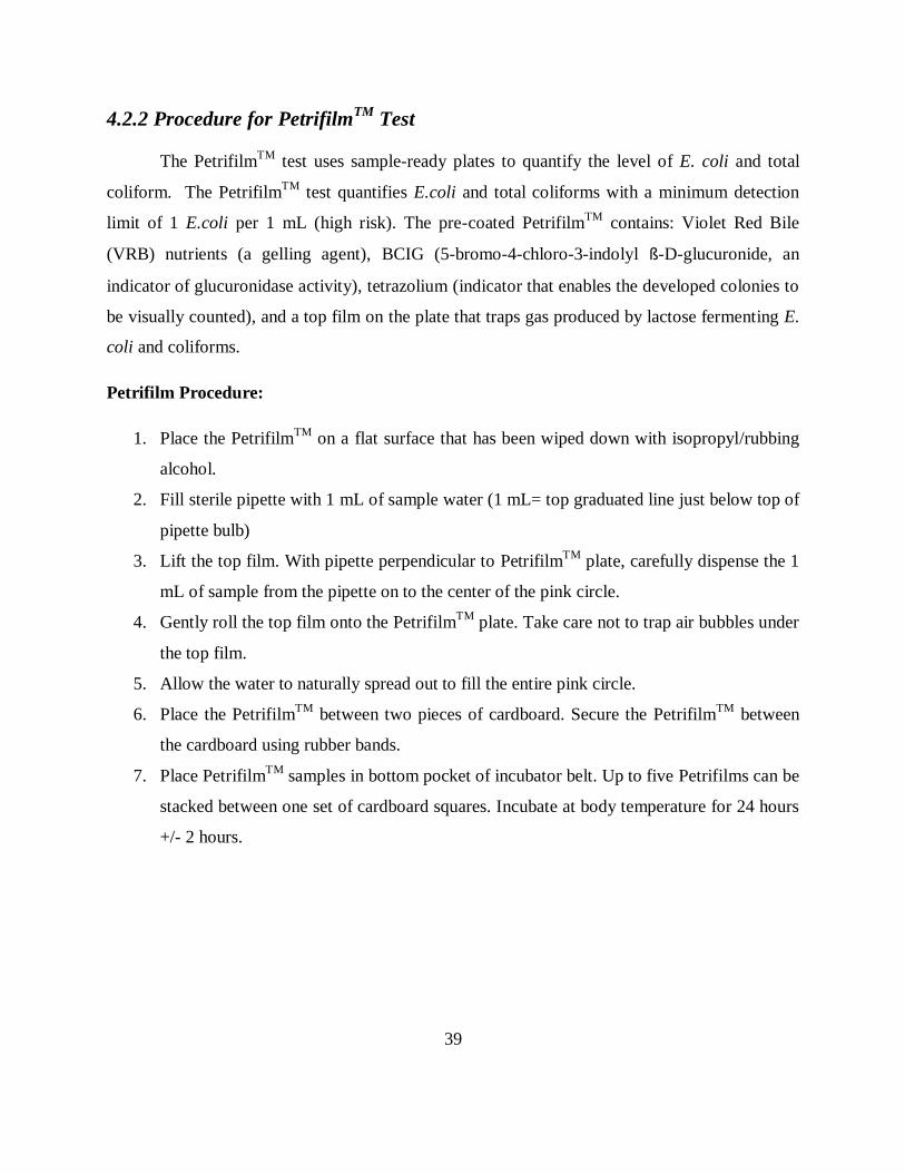
4.2.2 Procedure for PetrifilmTM
Test
The PetrifilmTM
test uses sample-ready plates to quantify the level of E. coli and total
coliform. The PetrifilmTM
test quantifies E.coli and total coliforms with a minimum detection
limit of 1 E.coli per 1 mL (high risk). The pre-coated PetrifilmTM
contains: Violet Red Bile
(VRB) nutrients (a gelling agent), BCIG (5-bromo-4-chloro-3-indolyl ß-D-glucuronide, an
indicator of glucuronidase activity), tetrazolium (indicator that enables the developed colonies to
be visually counted), and a top film on the plate that traps gas produced by lactose fermenting E.
coli and coliforms.
Petrifilm Procedure:
1. Place the PetrifilmTM
on a flat surface that has been wiped down with isopropyl/rubbing
alcohol.
2. Fill sterile pipette with 1 mL of sample water (1 mL= top graduated line just below top of
pipette bulb)
3. Lift the top film. With pipette perpendicular to PetrifilmTM
plate, carefully dispense the 1
mL of sample from the pipette on to the center of the pink circle.
4. Gently roll the top film onto the PetrifilmTM
plate. Take care not to trap air bubbles under
the top film.
5. Allow the water to naturally spread out to fill the entire pink circle.
6. Place the PetrifilmTM
between two pieces of cardboard. Secure the PetrifilmTM
between
the cardboard using rubber bands.
7. Place PetrifilmTM
samples in bottom pocket of incubator belt. Up to five Petrifilms can be
stacked between one set of cardboard squares. Incubate at body temperature for 24 hours
+/- 2 hours.
40
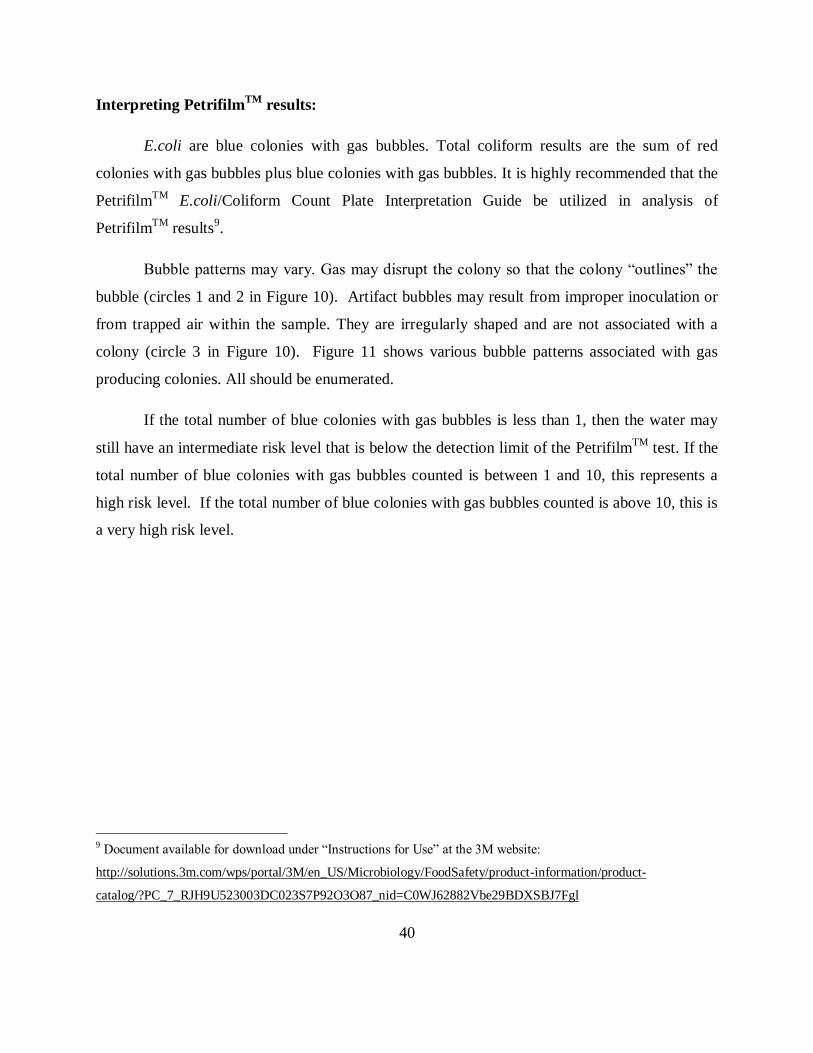
Interpreting PetrifilmTM
results:
E.coli are blue colonies with gas bubbles. Total coliform results are the sum of red
colonies with gas bubbles plus blue colonies with gas bubbles. It is highly recommended that the
PetrifilmTM
E.coli/Coliform Count Plate Interpretation Guide be utilized in analysis of
PetrifilmTM
results9.
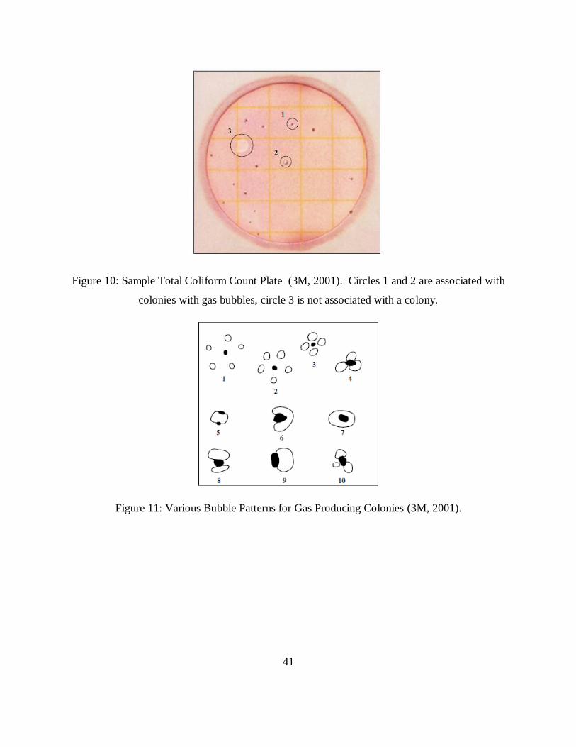
Bubble patterns may vary. Gas may disrupt the colony so that the colony “outlines” the
bubble (circles 1 and 2 in Figure 10). Artifact bubbles may result from improper inoculation or
from trapped air within the sample. They are irregularly shaped and are not associated with a
colony (circle 3 in Figure 10). Figure 11 shows various bubble patterns associated with gas
producing colonies. All should be enumerated.
If the total number of blue colonies with gas bubbles is less than 1, then the water may
still have an intermediate risk level that is below the detection limit of the PetrifilmTM
test. If the
total number of blue colonies with gas bubbles counted is between 1 and 10, this represents a
high risk level. If the total number of blue colonies with gas bubbles counted is above 10, this is
a very high risk level.
9 Document available for download under “Instructions for Use” at the 3M website:
http://solutions.3m.com/wps/portal/3M/en_US/Microbiology/FoodSafety/product-information/product-
catalog/?PC_7_RJH9U523003DC023S7P92O3O87_nid=C0WJ62882Vbe29BDXSBJ7Fgl
41
Figure 10: Sample Total Coliform Count Plate (3M, 2001). Circles 1 and 2 are associated with
colonies with gas bubbles, circle 3 is not associated with a colony.
Figure 11: Various Bubble Patterns for Gas Producing Colonies (3M, 2001).
42
4.2.3 Recommendations on Reading Colilert® and PetrifilmTM
Results
For the Colilert® test, the UV/black light test to determine fluorescence must be performed
in the dark (dark room, a closet, a bathroom, or outdoors at night). Otherwise, fluorescence will
not be able to be seen clearly.
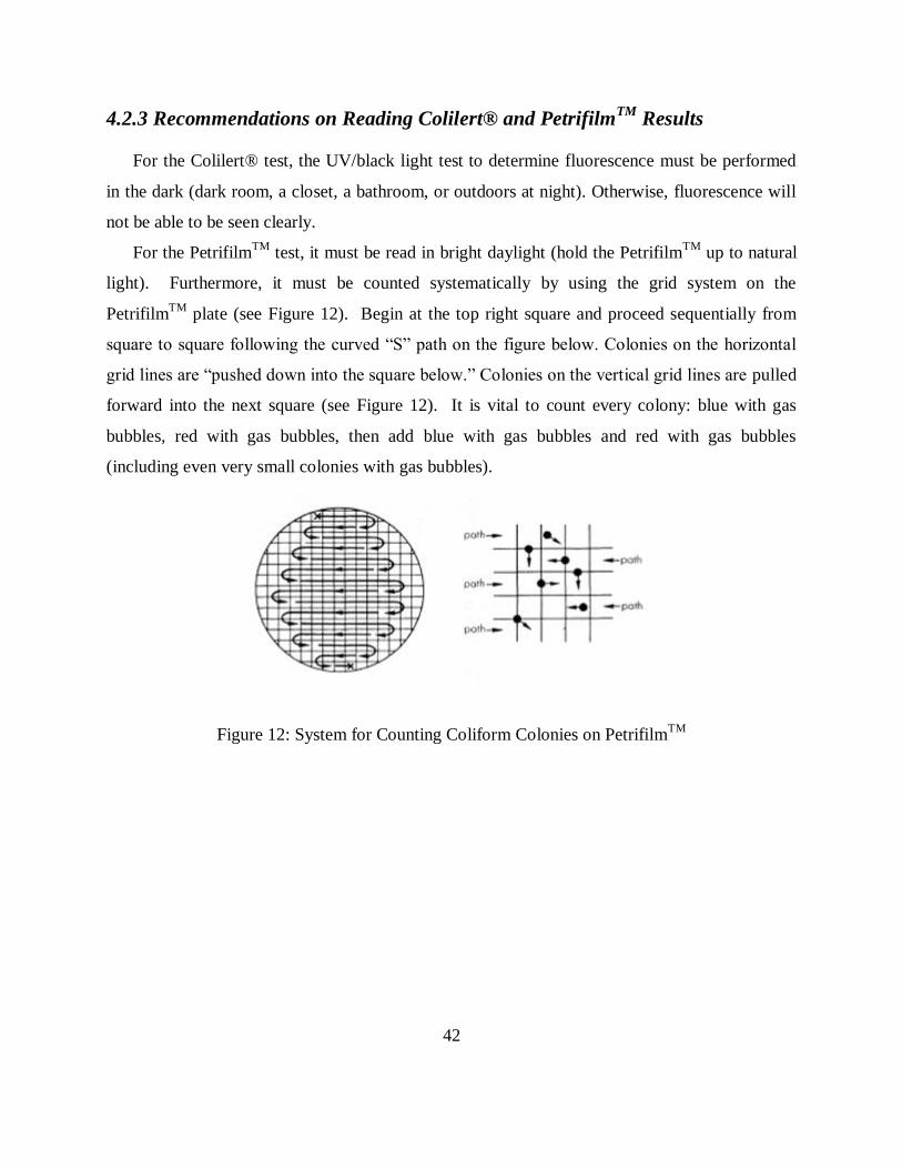
For the PetrifilmTM
test, it must be read in bright daylight (hold the PetrifilmTM
up to natural
light). Furthermore, it must be counted systematically by using the grid system on the
PetrifilmTM
plate (see Figure 12). Begin at the top right square and proceed sequentially from
square to square following the curved “S” path on the figure below. Colonies on the horizontal
grid lines are “pushed down into the square below.” Colonies on the vertical grid lines are pulled
forward into the next square (see Figure 12). It is vital to count every colony: blue with gas
bubbles, red with gas bubbles, then add blue with gas bubbles and red with gas bubbles
(including even very small colonies with gas bubbles).
Figure 12: System for Counting Coliform Colonies on PetrifilmTM
43
4.2.4 Determining Risk Levels from EC-Kit Results
For the purposes of prioritizing interventions at the regional level, it is important to
monitor the improvement or deterioration of drinking water supplies. In many developing
countries, a high proportion of small-community drinking-water systems fail to meet
requirements for water safety (World Health Organization, 2006). According to the WHO,
assigning a grading scheme is particularly useful for water sources where water quality testing
frequency is low. Furthermore, in locations where community water supplies are unchlorinated,
as was the case for non-Level 3 water sources in Capiz Province, they will inevitably contain
large numbers of total coliform bacteria. Therefore, it was recommended that the bacteriological
classification scheme should be based on thermotolerant (fecal) coliform bacteria or E.coli
(World Health Organization, 1997). For this study, analysis of microbiological water quality
data was divided into the WHO risk levels shown in Table 6.
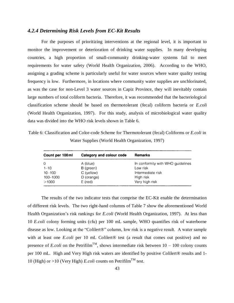
Table 6: Classification and Color-code Scheme for Thermotolerant (fecal) Coliforms or E.coli in
Water Supplies (World Health Organization, 1997)
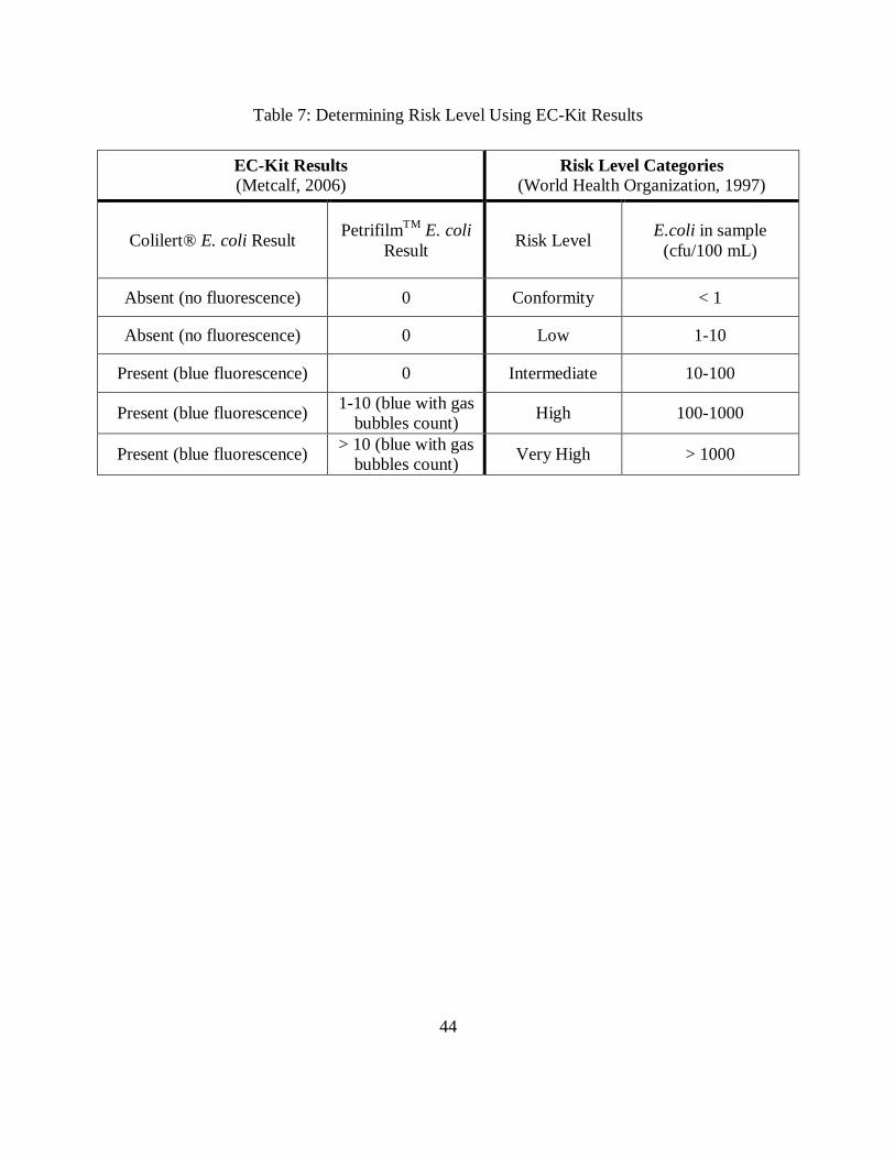
The results of the two indicator tests that comprise the EC-Kit enable the determination
of different risk levels. The two right-hand columns of Table 7 show the aforementioned World
Health Organization’s risk rankings for E.coli (World Health Organization, 1997). At less than
10 E.coli colony forming units (cfu) per 100 mL sample, WHO quantifies risk of waterborne
disease as low. Looking at the “Colilert®” column, low risk is a negative result. A water sample
with at least one E.coli per 10 mL Colilert® test (a result that comes out positive) and no
presence of E.coli on the PetrifilmTM
, shows intermediate risk between 10 – 100 colony counts
per 100 mL. High and Very High risk waters are identified by positive Colilert® results and 1-
10 (High) or >10 (Very High) E.coli counts on PetrifilmTM
test.
44
Table 7: Determining Risk Level Using EC-Kit Results
EC-Kit Results
(Metcalf, 2006) Risk Level Categories
(World Health Organization, 1997)
Colilert® E. coli Result Petrifilm
TM E. coli
Result Risk Level
E.coli in sample
(cfu/100 mL)
Absent (no fluorescence) 0 Conformity < 1
Absent (no fluorescence) 0 Low 1-10
Present (blue fluorescence) 0 Intermediate 10-100
Present (blue fluorescence) 1-10 (blue with gas
bubbles count) High 100-1000
Present (blue fluorescence) > 10 (blue with gas
bubbles count) Very High > 1000
45
4.3 Charles River Water Sampling
On April 4, 2010, the author collected water samples from the Charles River at the MIT
Sailing Pavilion, in Cambridge, Massachusetts. The samples were obtained in one location,
versus multiple locations (as was the case in Capiz Province). The purpose of the study was to
conduct a detailed, in-depth controlled experiment comparing the EC-Kit field test with the
Quanti-Tray® Standard Method with multiple sample dilutions, duplicates, and blanks. A
secondary purpose was to refine the comparison by running tests using Quanti-Tray®/2000
versus Quanti-Tray® (see Appendix C: Charles River Water Quality Results).
Charles River Water Sample Collection Procedure:
1. Rinse out sampling containers with Charles River water (the sampling vessels used in this
study were standard five-gallon plastic containers).
2. Collect sufficient Charles River Water (this study collected 10 gallons, which was more
than enough) and carry to the laboratory for testing.
3. Set up and label Quanti-Tray® and EC-Kit tests with date, dilution, and sample number.
4. Stir the Charles River water samples.
5. Dilute samples in sterile beakers with the appropriate volumes of deionized water. For
example, a dilution of 1/100 would have 1 mL of Charles River Water in 100 mL of
deionized of water.
a. Rinse beakers with deionized water in between each dilution.
b. Note: The dilutions should be conducted in increasing magnitude (e.g. 1/100 first,
followed by 2/100).
6. Conduct Quanti-Tray® and EC-Kit tests according to procedures detailed in Section 4.1
and 4.2.
7. Incubate for 24 hours using laboratory incubator.
46
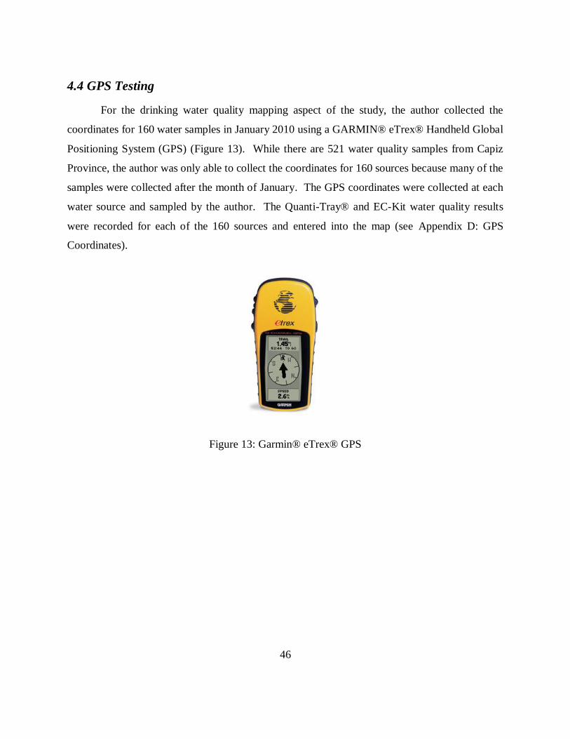
4.4 GPS Testing
For the drinking water quality mapping aspect of the study, the author collected the
coordinates for 160 water samples in January 2010 using a GARMIN® eTrex® Handheld Global
Positioning System (GPS) (Figure 13). While there are 521 water quality samples from Capiz
Province, the author was only able to collect the coordinates for 160 sources because many of the
samples were collected after the month of January. The GPS coordinates were collected at each
water source and sampled by the author. The Quanti-Tray® and EC-Kit water quality results
were recorded for each of the 160 sources and entered into the map (see Appendix D: GPS
Coordinates).
Figure 13: Garmin® eTrex® GPS
47
4.5 Statistical Analyses
The Capiz Province and Charles River water samples were analyzed statistically to
determine the accuracy of the water quality tests compared to the Standard Method, IDEXX
Quanti-Tray®. For all statistical analyses, STATA: Data Analysis and Statistical Software
(Version 11.0) was used.
One of the main difficulties encountered in the comparisons of Colilert®, PetrifilmTM
,
and the EC-Kit as a whole to Quanti-Tray® and Quanti-Tray®/2000 is the varying detection
limits per test. While the Colilert® 10-mL predispensed test reagent is identical to that used in
the Quanti-Tray® test, the difference is in the sample size (10-mL vs. 100-mL) and therefore in
the detection limits. The detection limit of the Colilert® 10-mL tubes is 10 cfu per 100 mL of
sample (a positive/present Colilert® result indicates 1 cfu per 10 mL sample, and hence 10 cfu
per 100 mL of sample). The detection limit of Quanti-Tray® is 200.5 MPN per 100 mL of
sample, whereas the detection limit of Quanti-Tray®/2000 is 2419 MPN per 100 mL of sample.
Another difficulty is the fact that the Colilert® test is a qualitative test and the PetrifilmTM
test is
enumerative. Statistical analyses of the two microbiological tests were conducted through the
use frequency distribution tables, otherwise known as contingency tables. Contingency tables
represent a method for analyzing categorical/nominal data (e.g. Presence/Absence, or WHO risk
levels) and are a simple procedure for reviewing how different categories are distributed in the
samples. The frequency distribution tables were then tested for statistical significance through
the chi-square test or Fisher’s exact test.
Statistical significance reports if it is unlikely a result occurred by chance, and establishes the
degree of confidence that one can have in making a inference from a sample to its parent
population (Meier, Brudney, & Bohte, 2009). The level of statistical significance is determined
through the use of a p-value (Rosner, 2006) as shown in Table 8.
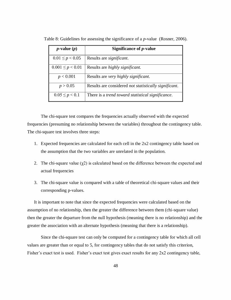
48
Table 8: Guidelines for assessing the significance of a p-value (Rosner, 2006).
p-value (p) Significance of p-value
0.01 ≤ p < 0.05 Results are significant.
0.001 ≤ p < 0.01 Results are highly significant.
p < 0.001 Results are very highly significant.
p > 0.05 Results are considered not statistically significant.
0.05 ≤ p < 0.1 There is a trend toward statistical significance.
The chi-square test compares the frequencies actually observed with the expected
frequencies (presuming no relationship between the variables) throughout the contingency table.
The chi-square test involves three steps:
1. Expected frequencies are calculated for each cell in the 2x2 contingency table based on
the assumption that the two variables are unrelated in the population.
2. The chi-square value (χ2) is calculated based on the difference between the expected and
actual frequencies
3. The chi-square value is compared with a table of theoretical chi-square values and their
corresponding p-values.
It is important to note that since the expected frequencies were calculated based on the
assumption of no relationship, then the greater the difference between them (chi-square value)
then the greater the departure from the null hypothesis (meaning there is no relationship) and the
greater the association with an alternate hypothesis (meaning that there is a relationship).
Since the chi-square test can only be computed for a contingency table for which all cell
values are greater than or equal to 5, for contingency tables that do not satisfy this criterion,
Fisher’s exact test is used. Fisher’s exact test gives exact results for any 2x2 contingency table,

49
but since it is more complicated to calculate, it is only used for tables with small cell values (less
than 5). The p-value determined from Fisher’s exact test is very similar to the chi-square test
(Rosner, 2006).
4.6 Limitations to the Study
One of the challenges in analyzing the Quanti-Tray and EC-Kit data for the Capiz
Province water samples was that the detection limits of the Quanti-Tray® used in the Philippines
is 200.5 MPN/100 mL of sample, whereas the detection limit of Quanti-Tray®/2000 used for
Charles River water samples is 2419 MPN/100 mL of sample.
The Quanti-Tray® was likely recommended to the Capiz Provincial Health Office by the
supplier/distributer because Capiz indicated they were testing drinking water samples. However,
the supplier/distributer may have been unaware of the potential that the E.coli contaminant levels
for the drinking water samples might fall in the range between 200 and >2000 cfu, or perhaps
even higher.
Meanwhile, the PetrifilmTM
has a higher detection limit. As seen in Table 7, detection of
one colony forming unit (cfu) on the PetrifilmTM
already places the water sample in the High or
Very High risk level category. The PetrifilmTM
’s inability to distinguish between Conformity,
Low, and Intermediate is one of the primary reasons for needing the additional 10-mL
predispensed Colilert® test in the EC-Kit.
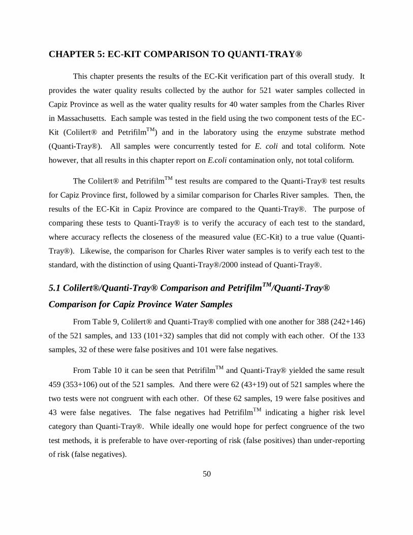
50
CHAPTER 5: EC-KIT COMPARISON TO QUANTI-TRAY®
This chapter presents the results of the EC-Kit verification part of this overall study. It
provides the water quality results collected by the author for 521 water samples collected in
Capiz Province as well as the water quality results for 40 water samples from the Charles River
in Massachusetts. Each sample was tested in the field using the two component tests of the EC-
Kit (Colilert® and PetrifilmTM
) and in the laboratory using the enzyme substrate method
(Quanti-Tray®). All samples were concurrently tested for E. coli and total coliform. Note
however, that all results in this chapter report on E.coli contamination only, not total coliform.
The Colilert® and PetrifilmTM
test results are compared to the Quanti-Tray® test results
for Capiz Province first, followed by a similar comparison for Charles River samples. Then, the
results of the EC-Kit in Capiz Province are compared to the Quanti-Tray®. The purpose of
comparing these tests to Quanti-Tray® is to verify the accuracy of each test to the standard,
where accuracy reflects the closeness of the measured value (EC-Kit) to a true value (Quanti-
Tray®). Likewise, the comparison for Charles River water samples is to verify each test to the
standard, with the distinction of using Quanti-Tray®/2000 instead of Quanti-Tray®.
5.1 Colilert®/Quanti-Tray® Comparison and PetrifilmTM
/Quanti-Tray®
Comparison for Capiz Province Water Samples
From Table 9, Colilert® and Quanti-Tray® complied with one another for 388 (242+146)
of the 521 samples, and 133 (101+32) samples that did not comply with each other. Of the 133
samples, 32 of these were false positives and 101 were false negatives.
From Table 10 it can be seen that PetrifilmTM
and Quanti-Tray® yielded the same result
459 (353+106) out of the 521 samples. And there were 62 (43+19) out of 521 samples where the
two tests were not congruent with each other. Of these 62 samples, 19 were false positives and
43 were false negatives. The false negatives had PetrifilmTM
indicating a higher risk level
category than Quanti-Tray®. While ideally one would hope for perfect congruence of the two
test methods, it is preferable to have over-reporting of risk (false positives) than under-reporting
of risk (false negatives).
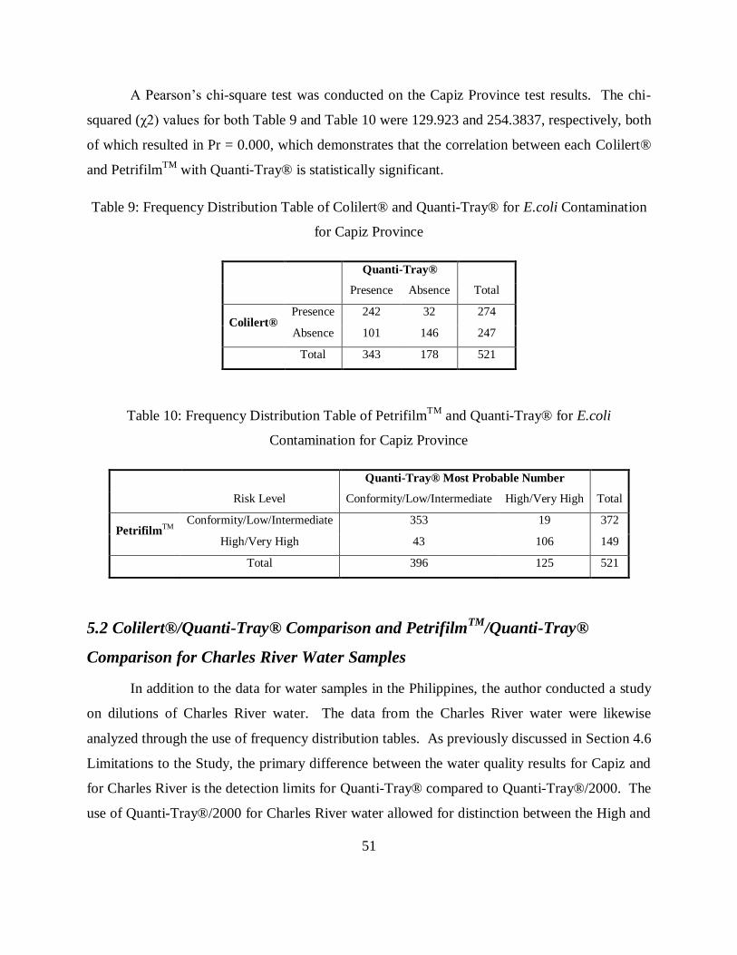
51
A Pearson’s chi-square test was conducted on the Capiz Province test results. The chi-
squared (χ2) values for both Table 9 and Table 10 were 129.923 and 254.3837, respectively, both
of which resulted in Pr = 0.000, which demonstrates that the correlation between each Colilert®
and PetrifilmTM
with Quanti-Tray® is statistically significant.
Table 9: Frequency Distribution Table of Colilert® and Quanti-Tray® for E.coli Contamination
for Capiz Province
Quanti-Tray®
Presence Absence Total
Colilert® Presence 242 32 274
Absence 101 146 247
Total 343 178 521
Table 10: Frequency Distribution Table of PetrifilmTM
and Quanti-Tray® for E.coli
Contamination for Capiz Province
Quanti-Tray® Most Probable Number
Risk Level Conformity/Low/Intermediate High/Very High Total
PetrifilmTM
Conformity/Low/Intermediate 353 19 372
High/Very High 43 106 149
Total 396 125 521
5.2 Colilert®/Quanti-Tray® Comparison and PetrifilmTM
/Quanti-Tray®
Comparison for Charles River Water Samples
In addition to the data for water samples in the Philippines, the author conducted a study
on dilutions of Charles River water. The data from the Charles River water were likewise
analyzed through the use of frequency distribution tables. As previously discussed in Section 4.6
Limitations to the Study, the primary difference between the water quality results for Capiz and
for Charles River is the detection limits for Quanti-Tray® compared to Quanti-Tray®/2000. The
use of Quanti-Tray®/2000 for Charles River water allowed for distinction between the High and
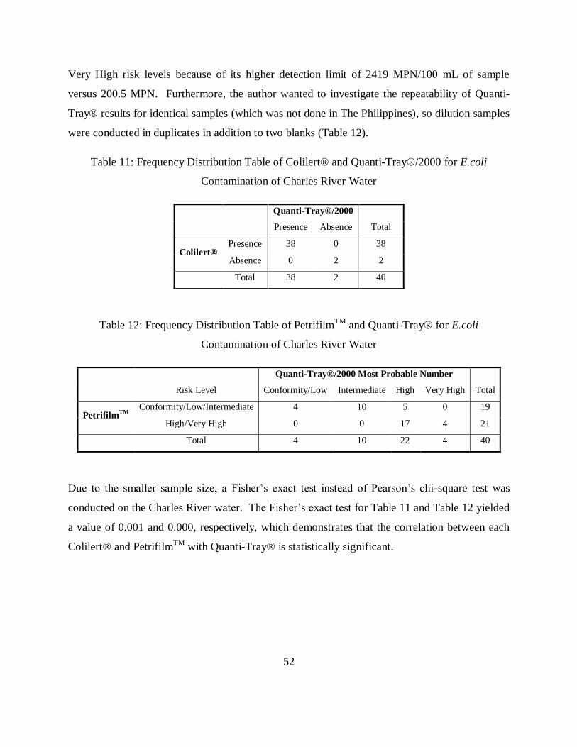
52
Very High risk levels because of its higher detection limit of 2419 MPN/100 mL of sample
versus 200.5 MPN. Furthermore, the author wanted to investigate the repeatability of Quanti-
Tray® results for identical samples (which was not done in The Philippines), so dilution samples
were conducted in duplicates in addition to two blanks (Table 12).
Table 11: Frequency Distribution Table of Colilert® and Quanti-Tray®/2000 for E.coli
Contamination of Charles River Water
Quanti-Tray®/2000
Presence Absence Total
Colilert® Presence 38 0 38
Absence 0 2 2
Total 38 2 40
Table 12: Frequency Distribution Table of PetrifilmTM
and Quanti-Tray® for E.coli
Contamination of Charles River Water
Quanti-Tray®/2000 Most Probable Number
Risk Level Conformity/Low Intermediate High Very High Total
PetrifilmTM
Conformity/Low/Intermediate 4 10 5 0 19
High/Very High 0 0 17 4 21
Total 4 10 22 4 40
Due to the smaller sample size, a Fisher’s exact test instead of Pearson’s chi-square test was
conducted on the Charles River water. The Fisher’s exact test for Table 11 and Table 12 yielded
a value of 0.001 and 0.000, respectively, which demonstrates that the correlation between each
Colilert® and PetrifilmTM
with Quanti-Tray® is statistically significant.
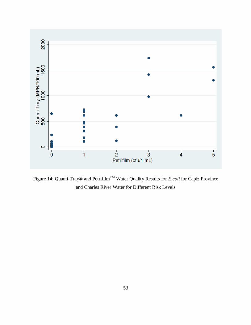
53
Figure 14: Quanti-Tray® and PetrifilmTM
Water Quality Results for E.coli for Capiz Province
and Charles River Water for Different Risk Levels
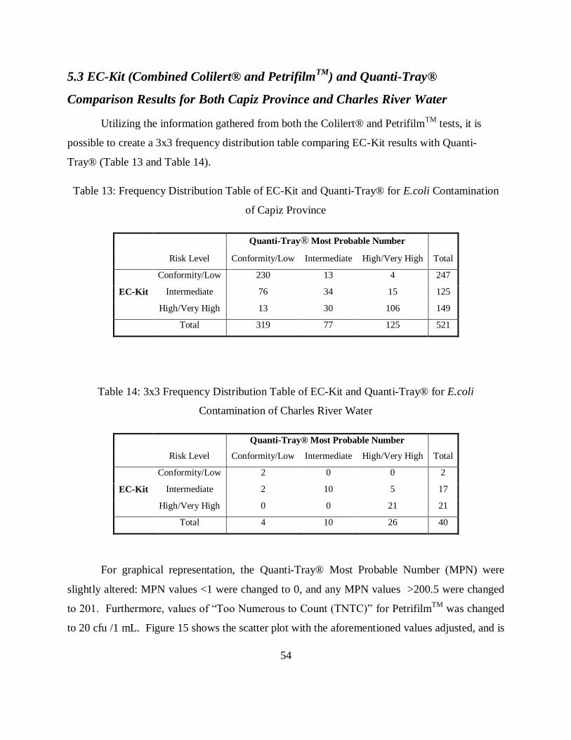
54
5.3 EC-Kit (Combined Colilert® and PetrifilmTM
) and Quanti-Tray®
Comparison Results for Both Capiz Province and Charles River Water
Utilizing the information gathered from both the Colilert® and PetrifilmTM
tests, it is
possible to create a 3x3 frequency distribution table comparing EC-Kit results with Quanti-
Tray® (Table 13 and Table 14).
Table 13: Frequency Distribution Table of EC-Kit and Quanti-Tray® for E.coli Contamination
of Capiz Province
Quanti-Tray® Most Probable Number
Risk Level Conformity/Low Intermediate High/Very High Total
EC-Kit
Conformity/Low 230 13 4 247
Intermediate 76 34 15 125
High/Very High 13 30 106 149
Total 319 77 125 521
Table 14: 3x3 Frequency Distribution Table of EC-Kit and Quanti-Tray® for E.coli
Contamination of Charles River Water
Quanti-Tray® Most Probable Number
Risk Level Conformity/Low Intermediate High/Very High Total
EC-Kit
Conformity/Low 2 0 0 2
Intermediate 2 10 5 17
High/Very High 0 0 21 21
Total 4 10 26 40
For graphical representation, the Quanti-Tray® Most Probable Number (MPN) were
slightly altered: MPN values <1 were changed to 0, and any MPN values >200.5 were changed
to 201. Furthermore, values of “Too Numerous to Count (TNTC)” for PetrifilmTM
was changed
to 20 cfu /1 mL. Figure 15 shows the scatter plot with the aforementioned values adjusted, and is
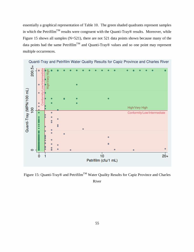
55
essentially a graphical representation of Table 10. The green shaded quadrants represent samples
in which the PetrifilmTM
results were congruent with the Quanti-Tray® results. Moreover, while
Figure 15 shows all samples (N=521), there are not 521 data points shown because many of the
data points had the same PetrifilmTM
and Quanti-Tray® values and so one point may represent
multiple occurrences.
Figure 15: Quanti-Tray® and PetrifilmTM
Water Quality Results for Capiz Province and Charles
River
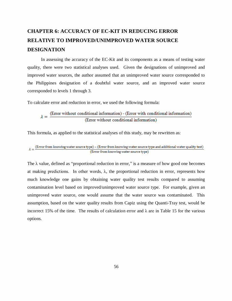
56
CHAPTER 6: ACCURACY OF EC-KIT IN REDUCING ERROR
RELATIVE TO IMPROVED/UNIMPROVED WATER SOURCE
DESIGNATION
In assessing the accuracy of the EC-Kit and its components as a means of testing water
quality, there were two statistical analyses used. Given the designations of unimproved and
improved water sources, the author assumed that an unimproved water source corresponded to
the Philippines designation of a doubtful water source, and an improved water source
corresponded to levels 1 through 3.
To calculate error and reduction in error, we used the following formula:
This formula, as applied to the statistical analyses of this study, may be rewritten as:
The λ value, defined as “proportional reduction in error,” is a measure of how good one becomes
at making predictions. In other words, λ, the proportional reduction in error, represents how
much knowledge one gains by obtaining water quality test results compared to assuming
contamination level based on improved/unimproved water source type. For example, given an
unimproved water source, one would assume that the water source was contaminated. This
assumption, based on the water quality results from Capiz using the Quanti-Tray test, would be
incorrect 15% of the time. The results of calculation error and λ are in Table 15 for the various
options.
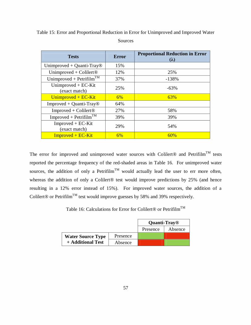
57
Table 15: Error and Proportional Reduction in Error for Unimproved and Improved Water
Sources
Tests Error Proportional Reduction in Error
(λ)
Unimproved + Quanti-Tray® 15%
Unimproved + Colilert® 12% 25%
Unimproved + PetrifilmTM
37% -138%
Unimproved + EC-Kit
(exact match) 25% -63%
Unimproved + EC-Kit 6% 63%
Improved + Quanti-Tray® 64%
Improved + Colilert® 27% 58%
Improved + PetrifilmTM
39% 39%
Improved + EC-Kit
(exact match) 29% 54%
Improved + EC-Kit 6% 60%
The error for improved and unimproved water sources with Colilert® and PetrifilmTM
tests
reported the percentage frequency of the red-shaded areas in Table 16. For unimproved water
sources, the addition of only a PetrifilmTM
would actually lead the user to err more often,
whereas the addition of only a Colilert® test would improve predictions by 25% (and hence
resulting in a 12% error instead of 15%). For improved water sources, the addition of a
Colilert® or PetrifilmTM
test would improve guesses by 58% and 39% respectively.
Table 16: Calculations for Error for Colilert® or PetrifilmTM
Quanti-Tray®
Presence Absence
Water Source Type
+ Additional Test
Presence
Absence
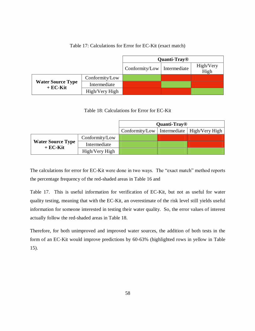
58
Table 17: Calculations for Error for EC-Kit (exact match)
Quanti-Tray®
Conformity/Low Intermediate
High/Very
High
Water Source Type
+ EC-Kit
Conformity/Low
Intermediate
High/Very High
Table 18: Calculations for Error for EC-Kit
Quanti-Tray®
Conformity/Low Intermediate High/Very High
Water Source Type
+ EC-Kit
Conformity/Low
Intermediate
High/Very High
The calculations for error for EC-Kit were done in two ways. The “exact match” method reports
the percentage frequency of the red-shaded areas in Table 16 and
Table 17. This is useful information for verification of EC-Kit, but not as useful for water
quality testing, meaning that with the EC-Kit, an overestimate of the risk level still yields useful
information for someone interested in testing their water quality. So, the error values of interest
actually follow the red-shaded areas in Table 18.
Therefore, for both unimproved and improved water sources, the addition of both tests in the
form of an EC-Kit would improve predictions by 60-63% (highlighted rows in yellow in Table
15).
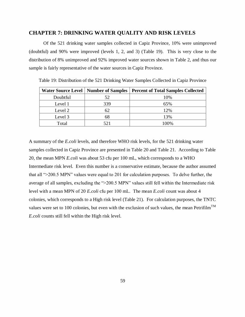
59
CHAPTER 7: DRINKING WATER QUALITY AND RISK LEVELS
Of the 521 drinking water samples collected in Capiz Province, 10% were unimproved
(doubtful) and 90% were improved (levels 1, 2, and 3) (Table 19). This is very close to the
distribution of 8% unimproved and 92% improved water sources shown in Table 2, and thus our
sample is fairly representative of the water sources in Capiz Province.
Table 19: Distribution of the 521 Drinking Water Samples Collected in Capiz Province
Water Source Level Number of Samples Percent of Total Samples Collected
Doubtful 52 10%
Level 1 339 65%
Level 2 62 12%
Level 3 68 13%
Total 521 100%
A summary of the E.coli levels, and therefore WHO risk levels, for the 521 drinking water
samples collected in Capiz Province are presented in Table 20 and Table 21. According to Table
20, the mean MPN E.coli was about 53 cfu per 100 mL, which corresponds to a WHO
Intermediate risk level. Even this number is a conservative estimate, because the author assumed
that all “>200.5 MPN” values were equal to 201 for calculation purposes. To delve further, the
average of all samples, excluding the “>200.5 MPN” values still fell within the Intermediate risk
level with a mean MPN of 20 E.coli cfu per 100 mL. The mean E.coli count was about 4
colonies, which corresponds to a High risk level (Table 21). For calculation purposes, the TNTC
values were set to 100 colonies, but even with the exclusion of such values, the mean PetrifilmTM
E.coli counts still fell within the High risk level.
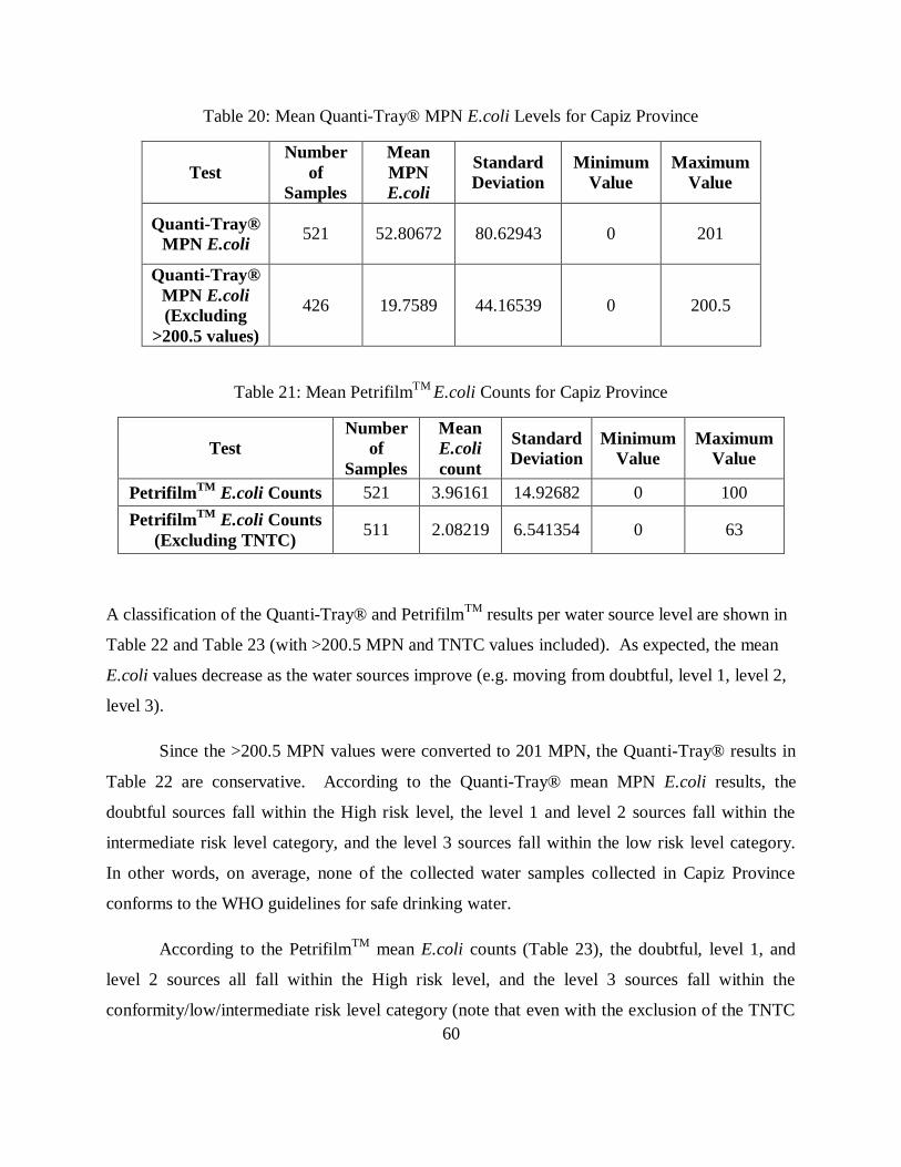
60
Table 20: Mean Quanti-Tray® MPN E.coli Levels for Capiz Province
Test
Number
of
Samples
Mean
MPN
E.coli
Standard
Deviation
Minimum
Value
Maximum
Value
Quanti-Tray®
MPN E.coli 521 52.80672 80.62943 0 201
Quanti-Tray®
MPN E.coli
(Excluding
>200.5 values)
426 19.7589 44.16539 0 200.5
Table 21: Mean PetrifilmTM
E.coli Counts for Capiz Province
Test
Number
of
Samples
Mean
E.coli
count
Standard
Deviation
Minimum
Value
Maximum
Value
PetrifilmTM
E.coli Counts 521 3.96161 14.92682 0 100
PetrifilmTM
E.coli Counts
(Excluding TNTC) 511 2.08219 6.541354 0 63
A classification of the Quanti-Tray® and PetrifilmTM
results per water source level are shown in
Table 22 and Table 23 (with >200.5 MPN and TNTC values included). As expected, the mean
E.coli values decrease as the water sources improve (e.g. moving from doubtful, level 1, level 2,
level 3).
Since the >200.5 MPN values were converted to 201 MPN, the Quanti-Tray® results in
Table 22 are conservative. According to the Quanti-Tray® mean MPN E.coli results, the
doubtful sources fall within the High risk level, the level 1 and level 2 sources fall within the
intermediate risk level category, and the level 3 sources fall within the low risk level category.
In other words, on average, none of the collected water samples collected in Capiz Province
conforms to the WHO guidelines for safe drinking water.
According to the PetrifilmTM
mean E.coli counts (Table 23), the doubtful, level 1, and
level 2 sources all fall within the High risk level, and the level 3 sources fall within the
conformity/low/intermediate risk level category (note that even with the exclusion of the TNTC
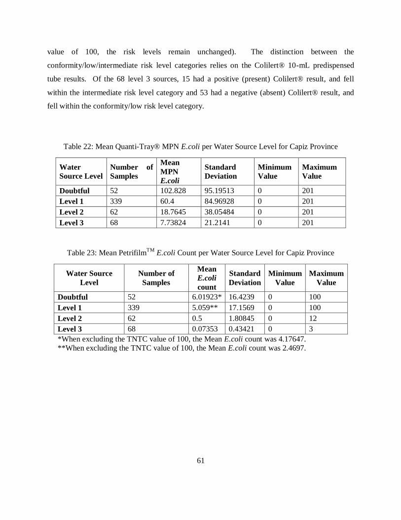
61
value of 100, the risk levels remain unchanged). The distinction between the
conformity/low/intermediate risk level categories relies on the Colilert® 10-mL predispensed
tube results. Of the 68 level 3 sources, 15 had a positive (present) Colilert® result, and fell
within the intermediate risk level category and 53 had a negative (absent) Colilert® result, and
fell within the conformity/low risk level category.
Table 22: Mean Quanti-Tray® MPN E.coli per Water Source Level for Capiz Province
Water
Source Level
Number of
Samples
Mean
MPN
E.coli
Standard
Deviation
Minimum
Value
Maximum
Value
Doubtful 52 102.828 95.19513 0 201
Level 1 339 60.4 84.96928 0 201
Level 2 62 18.7645 38.05484 0 201
Level 3 68 7.73824 21.2141 0 201
Table 23: Mean PetrifilmTM
E.coli Count per Water Source Level for Capiz Province
Water Source
Level
Number of
Samples
Mean
E.coli
count
Standard
Deviation
Minimum
Value
Maximum
Value
Doubtful 52 6.01923* 16.4239 0 100
Level 1 339 5.059** 17.1569 0 100
Level 2 62 0.5 1.80845 0 12
Level 3 68 0.07353 0.43421 0 3
*When excluding the TNTC value of 100, the Mean E.coli count was 4.17647.
**When excluding the TNTC value of 100, the Mean E.coli count was 2.4697.
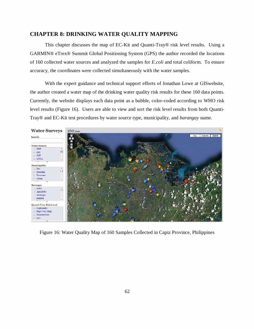
62
CHAPTER 8: DRINKING WATER QUALITY MAPPING
This chapter discusses the map of EC-Kit and Quanti-Tray® risk level results. Using a
GARMIN® eTrex® Summit Global Positioning System (GPS) the author recorded the locations
of 160 collected water sources and analyzed the samples for E.coli and total coliform. To ensure
accuracy, the coordinates were collected simultaneously with the water samples.
With the expert guidance and technical support efforts of Jonathan Lowe at GISwebsite,
the author created a water map of the drinking water quality risk results for these 160 data points.
Currently, the website displays each data point as a bubble, color-coded according to WHO risk
level results (Figure 16). Users are able to view and sort the risk level results from both Quanti-
Tray® and EC-Kit test procedures by water source type, municipality, and barangay name.
Figure 16: Water Quality Map of 160 Samples Collected in Capiz Province, Philippines
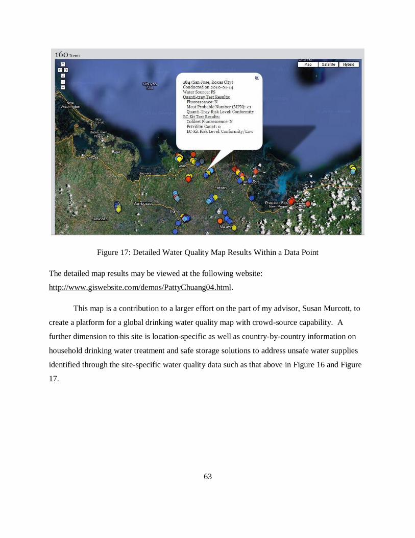
63
Figure 17: Detailed Water Quality Map Results Within a Data Point
The detailed map results may be viewed at the following website:
http://www.giswebsite.com/demos/PattyChuang04.html.
This map is a contribution to a larger effort on the part of my advisor, Susan Murcott, to
create a platform for a global drinking water quality map with crowd-source capability. A
further dimension to this site is location-specific as well as country-by-country information on
household drinking water treatment and safe storage solutions to address unsafe water supplies
identified through the site-specific water quality data such as that above in Figure 16 and Figure
17.
64
CHAPTER 9: CONCLUSION AND RECOMMENDATIONS
9.1 EC-Kit Verification and Testing
From the chi-square and Fischer’s exact tests, we see that each component of EC-Kit and
the entire kit itself is correlated to Quanti-Tray® in a statistically significant way. Furthermore,
from the calculations of error and proportional reduction in error for unimproved and improved
water sources, it possible to make better predictions with just the use of the Colilert® test, but
not just the use of the PetrifilmTM
test. This is due to the detection limits for PetrifilmTM
being
much higher than Colilert®, namely positive PetrifilmTM
results fall within the High and Very
High risk level categories, whereas positive Colilert® results fall within the Intermediate, High,
and Very High risk level categories. Most importantly, the two test set of the EC-Kit allows for
the best reduction in error, with a proportional reduction in error of 63% for unimproved water
sources and 60% for improved water sources.
9.2 Drinking Water Quality Mapping
The water quality mapping project is ongoing and the maps will be updated and modified
in the future by the author, Jonathan Lowe, and Susan Murcott. The mapping coordinates were
only as accurate as the GPS would allow (typical accuracy <15 meters feet range), especially in
the rural areas of Capiz Province. Future updates to the map could allow users to input
additional information, such as results from water quality tests beyond Quanti-Tray® and EC-
Kit. Additionally, less technical information would be useful for users interested in mapping,
such as displaying photos of the water source types, and short summaries of site-specific water
sources.
9.3 Summary
Risk level data according to Escherichia coli and total coliform levels has been collected
for drinking water sources for different locations and source types in Capiz Province. Quanti-
Tray® results revealed that of the 521 water samples collected, none of the sources conformed to
the WHO Guidelines for Drinking Water Quality. The details of each water sample may be
found in Appendix B: Water Quality Results, Sorted by Municipality.
65
Statistical analyses comparing the EC-Kit with Quanti-Tray® revealed that while the EC-
Kit does not exactly match the Quanti-Tray® results, it still provides useful information for
assessing at-risk water sources.
Furthermore, the basis for the Phlippines component of the global drinking water quality
map has been created, and further modifications and updates to the map will be made in the
future.
9.4 Recommendations for Future Studies
Due to the limitations present in the detection limits for Quanti-Tray® and PetrifilmTM
,
future projects verifying the EC-Kit are recommended to use Quanti-Tray®/2000.
In the author’s field work in Capiz, one of the primary complications was with the field
usage of the EC-Kit. Trainees of the EC-Kit attended a one-day workshop, and the training at
this workshop was not complete enough for field tests to commence. The chief problem may
have been that the training took place in May; however, due to unavoidable delays, the test
program itself could not begin until December. Moreover, the initial version of the EC-Kit
instructions lacked information regarding quality control procedures, and did not sufficiently
emphasize the need to maintain sterile conditions when collecting water samples for the EC-Kit.
Furthermore, there were no photos included with the instructions to help illustrate each step.
Since then, the author and her thesis advisor have modified the EC-Kit instructions (see
Appendix E: EC-Kit Instructions).
Future workshops in the EC-Kit should allow users to have a “trial” field testing, and a
follow-up workshop to address any questions or confusion about the methods and interpretation
of results. In particular, the author noticed that users of the EC-Kit were especially perplexed
regarding how to properly perform the fluorescence readings for the Colilert® test and the
PetrifilmTM
gas-forming colony counts. The author advises future users of the EC-Kit to
describe the Colilert® results as “milky, blue” fluorescence, and to emphasize reading
PetrifilmTM
results held up to proper daylight or bright lighting, so as to visibly notice the gas
bubble formations. In addition, it is highly recommended that the PetrifilmTM
E.coli/Coliform
66
Count Plate Interpretation Guide be utilized in analysis of PetrifilmTM
results10
. A possible
method for future workshops could have trainees in pairs or small groups, and have each member
individually count the blue colonies with gas bubbles, and have the group members compare
their counts. This would highlight the need to only count the colonies with gas bubbles, not
colonies without gas bubbles, and also introduce the concept of having a “double-check” count.
10 Document available for download under “Instructions for Use” at the 3M website:
http://solutions.3m.com/wps/portal/3M/en_US/Microbiology/FoodSafety/product-information/product-
catalog/?PC_7_RJH9U523003DC023S7P92O3O87_nid=C0WJ62882Vbe29BDXSBJ7Fgl
67
CHAPTER 10: REFERENCES
3M. (2001). Petrifilm™ E.coli/Coliform Count Plates Interpretation Guide. Retrieved from
http://multimedia.3m.com/mws/mediawebserver?mwsId=66666UuZjcFSLXTt4XMa4xTaEVuQ
EcuZgVs6EVs6E666666--
APHA, WEF, AWWA. (2005). Standard Methods for the Examination of Water and Wastewater
(21 ed.). Washington D.C.: American Public Health Association, Water Environment Federation,
and American Water Works Association.
Benaman, J., Shoemaker, C. A., & Haith, D. A. (2005). Calibration and Validation of Soil and
Water Assessment Tool on an Agricultural Watershed in Upstate New York. Journal of
Hydrologic Engineering , 10 (5), 363-374.
Central Intelligence Agency. (2010). The World Factbook.
Chao, K.-K., Chao, C.-C. C., & Chao, W.-L. (2004). Evaluation of Colilert-18 for Detection of
Coliforms and Eschericha coli in Subtropical Freshwater. Applied and Environmental
Microbiology , 70 (2), 1242-1244.
Doyle, M. P., & Erickson, M. C. (2006). Closing the Door on the Fecal Coliform Assay. Microbe
, 1 (4), 162-163.
Fricker, E. J., Illingworth, K. S., & Fricker, C. R. (1997). Use of Two Formulations of Colilert
and Quanti-Tray for Assessment of the Bacteriological Quality of Water. Water Research , 31
(10), 2495-2499.
Gassman, P. W., Reyes, M. R., Green, C. H., & Arnold, J. G. (2007). The Soil and Water
Assessment Tool: Historical Development, Applications, and Future Research Directions. Center
for Agricultural and Rural Development (CARD) .
IDEXX. (2009). IDEXX Water Microbiology Product Catalog. Retrieved December 2, 2009,
from IDEXX Laboratories - Coliform and E.coli Test Comparison:
http://www.idexx.com/pubwebresources/pdf/en_us/water/0971127.pdf
68
Lifshitz, R., & Joshi, R. (1997). Comparison of the Novel ColiPlate Kit and the Standard
Membrane Filter Technique for Enumerating Total Coliforms and Escherichia coli Bacteria in
Water. Retrieved from Bluewater Biosciences Inc.:
http://www.bluewaterbiosciences.com/products_coliplate.html
Mack, K., & Hewison, K. (1988). Report No. 47: Evaluation of a Hydrogen Sulfide Screening
Test. Thai-Australian Northeast village water resource project.
Meier, K. J., Brudney, J. L., & Bohte, J. (2009). Applied Statistics for Public and Nonprofit
Administration. Thomson-Wadsworth.
Metcalf, R. (2006). Powerpoint Presentation. The Portable Microbiology Laboratory:
Revolutionizing Point Source Water Testing in Africa . Sacramento, California.
Olson, B. H., Clark, D. L., Milner, B. B., Stewart, M. H., & Wolfe, R. L. (1991). Total Coliform
Detection in Drinking Water: Comparison of Membrane Filtration with Colilert and Coliquik.
Applied and Environmental Microbiology , 57 (5), 1535-1539.
Rosner, B. (2006). Fundamentals of Biostatisics, 5th edition. Belmont, CA: Thomson-
Brooks/Cole.
Schraft, H., & Watterworth, L. A. (2005). Enumeration of heterotrophs, fecal coliforms and
Escherichia coli in water: comparison of 3M Petrifilm plates with standard plating procedures.
Journal of Microbiological Methods , 60 (3), 335– 342.
Solar Cookers International (Safe Water, Kenya). (2007). Retrieved December 2, 2009, from
Solar Cookers International: http://www.solarcookers.org/programs/safewater.html
The Official Government Portal of the Republic of the Philippines. (2010). Retrieved from
http://www.gov.ph/
The Republic of Philippines Department of Health. (2007). Local Water Utilities Administration.
Retrieved from Technical matters, papers, etc. on Philippines water supply:
http://www.lwua.gov.ph/tech_mattrs/Philippine%20National%20Standards%20for%20Drinking
%20Water%202007.doc

69
The Republic of the Philippines Department of Health. (1976). The Code of Sanitation of the
Philippines. Retrieved from http://www2.doh.gov.ph/code_sanitation_phils.htm
Thermalindo. (2007). Online Catalog: Microbiology. Retrieved December 2, 2009, from PT.
Thermalindo Sarana Laboratoria:
http://www.thermalindo.com/online_catalog_detail.asp?categoryid=118&productid=441
Trottier, S. (2010). Study of Four New, Field-Based, Microbiological Tests: Verification of the
Hydrogen Sulfide (H2S), EasyGel®, Colilert and Petrifilm Tests.
UNICEF. (2007). Sub-Regional Data for Capiz, , Multi-Indicator Cluster Survey (MICS).
United Nations. (2000). Millenium Development Goals. United Nations Millenium Declaration.
New York City.
United Nations: The Right to Water. (2009). Independent Expert on the Issue of Human Rights
Obligations Related to Safe Drinking Wwater and Sanitation. Human Rights Council, 12th
Session.
United States Department of State. (2010, 04). Philippines. Retrieved from
http://www.state.gov/r/pa/ei/bgn/2794.htm
Vail, J. H., Morgan, R., Merino, C. R., Gonzales, F., Miller, R., & Ram, J. L. (2003).
Enumeration of Waterborne Escherichia coli with Petrifilm Plates: Comparison to Standard
Methods. Journal of Environmental Quality , 32 (1), 368-373.
WHO/UNICEF Joint Monitoring Programme for Water Supply and Sanitation. (2005). Water for
Life: Making It Happen. Geneva: World Health Organization and UNICEF.
WHO/UNICEF. (2010). Progress on Sanitation and Drinking-Water 2010 Update.
World Bank. (2006, February). CEPF and Poverty Reduction: A Review of the Philippines CEPF
Portfolio. Retrieved from
http://www.cepf.net/Documents/povertyreduction_philippines_feb06.pdf
World Health Organization. (1997). Guidelines for Drinking Water Quality (2 ed., Vol. 3).

70
World Health Organization. (1997). Guidelines for Drinking Water Quality (2nd ed., Vol. III).
Geneva: WHO.
World Health Organization. (2006). Guidelines for Drinking-Water Quality (3 ed., Vol. 1).

71
APPENDICES
72
Appendix A: IDEXX 51-Well Quanti-Tray® MPN Table
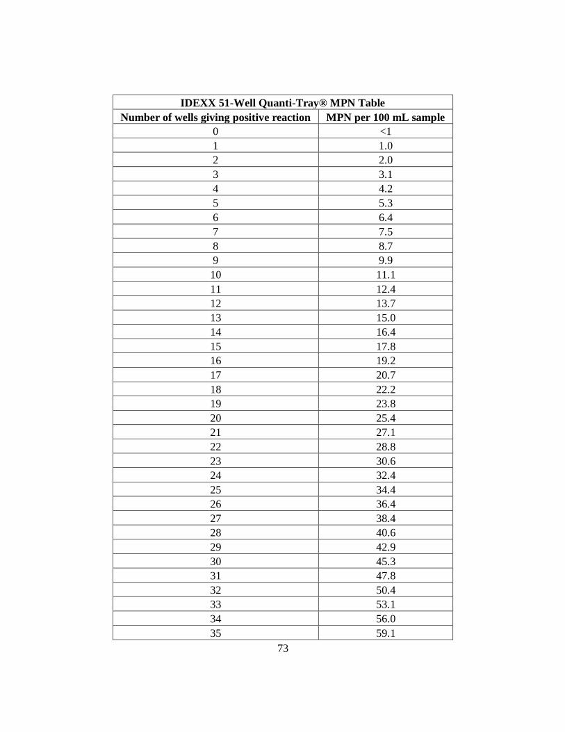
73
IDEXX 51-Well Quanti-Tray® MPN Table
Number of wells giving positive reaction MPN per 100 mL sample
0 <1
1 1.0
2 2.0
3 3.1
4 4.2
5 5.3
6 6.4
7 7.5
8 8.7
9 9.9
10 11.1
11 12.4
12 13.7
13 15.0
14 16.4
15 17.8
16 19.2
17 20.7
18 22.2
19 23.8
20 25.4
21 27.1
22 28.8
23 30.6
24 32.4
25 34.4
26 36.4
27 38.4
28 40.6
29 42.9
30 45.3
31 47.8
32 50.4
33 53.1
34 56.0
35 59.1
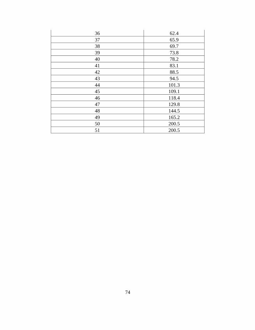
74
36 62.4
37 65.9
38 69.7
39 73.8
40 78.2
41 83.1
42 88.5
43 94.5
44 101.3
45 109.1
46 118.4
47 129.8
48 144.5
49 165.2
50 200.5
51 200.5
75
Appendix B: Water Quality Results, Sorted by Municipality
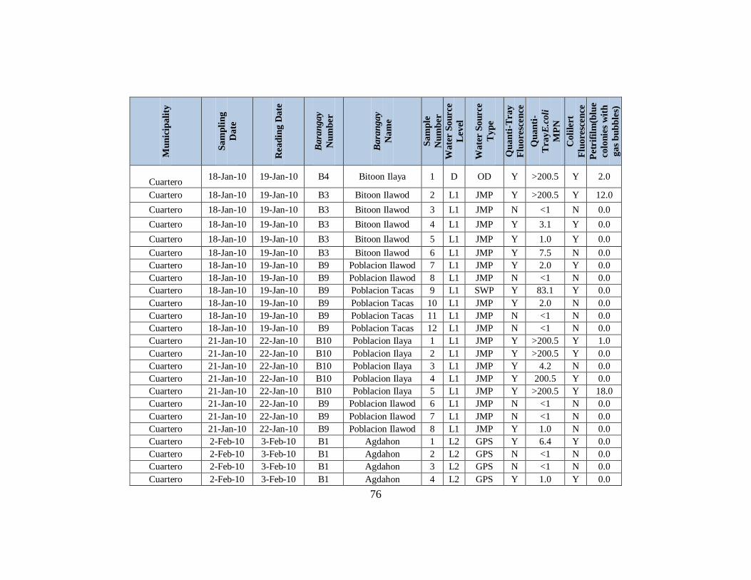
76
Mu
nic
ipa
lity
Sa
mp
lin
g
Da
te
Rea
din
g D
ate
Ba
ran
ga
y
Nu
mb
er
Ba
ran
ga
y
Na
me
Sa
mp
le
Nu
mb
er
Wa
ter S
ou
rce
Lev
el
Wa
ter S
ou
rce
Ty
pe
Qu
an
ti-T
ra
y
Flu
ore
scen
ce
Qu
an
ti-
Tra
yE
.co
li
MP
N
Co
lile
rt
Flu
ore
scen
ce
Petr
ifil
m(b
lue
co
lon
ies
wit
h
ga
s b
ub
ble
s)
Cuartero 18-Jan-10 19-Jan-10 B4 Bitoon Ilaya 1 D OD Y >200.5 Y 2.0
Cuartero 18-Jan-10 19-Jan-10 B3 Bitoon Ilawod 2 L1 JMP Y >200.5 Y 12.0
Cuartero 18-Jan-10 19-Jan-10 B3 Bitoon Ilawod 3 L1 JMP N <1 N 0.0
Cuartero 18-Jan-10 19-Jan-10 B3 Bitoon Ilawod 4 L1 JMP Y 3.1 Y 0.0
Cuartero 18-Jan-10 19-Jan-10 B3 Bitoon Ilawod 5 L1 JMP Y 1.0 Y 0.0
Cuartero 18-Jan-10 19-Jan-10 B3 Bitoon Ilawod 6 L1 JMP Y 7.5 N 0.0
Cuartero 18-Jan-10 19-Jan-10 B9 Poblacion Ilawod 7 L1 JMP Y 2.0 Y 0.0
Cuartero 18-Jan-10 19-Jan-10 B9 Poblacion Ilawod 8 L1 JMP N <1 N 0.0
Cuartero 18-Jan-10 19-Jan-10 B9 Poblacion Tacas 9 L1 SWP Y 83.1 Y 0.0
Cuartero 18-Jan-10 19-Jan-10 B9 Poblacion Tacas 10 L1 JMP Y 2.0 N 0.0
Cuartero 18-Jan-10 19-Jan-10 B9 Poblacion Tacas 11 L1 JMP N <1 N 0.0
Cuartero 18-Jan-10 19-Jan-10 B9 Poblacion Tacas 12 L1 JMP N <1 N 0.0
Cuartero 21-Jan-10 22-Jan-10 B10 Poblacion Ilaya 1 L1 JMP Y >200.5 Y 1.0
Cuartero 21-Jan-10 22-Jan-10 B10 Poblacion Ilaya 2 L1 JMP Y >200.5 Y 0.0
Cuartero 21-Jan-10 22-Jan-10 B10 Poblacion Ilaya 3 L1 JMP Y 4.2 N 0.0
Cuartero 21-Jan-10 22-Jan-10 B10 Poblacion Ilaya 4 L1 JMP Y 200.5 Y 0.0
Cuartero 21-Jan-10 22-Jan-10 B10 Poblacion Ilaya 5 L1 JMP Y >200.5 Y 18.0
Cuartero 21-Jan-10 22-Jan-10 B9 Poblacion Ilawod 6 L1 JMP N <1 N 0.0
Cuartero 21-Jan-10 22-Jan-10 B9 Poblacion Ilawod 7 L1 JMP N <1 N 0.0
Cuartero 21-Jan-10 22-Jan-10 B9 Poblacion Ilawod 8 L1 JMP Y 1.0 N 0.0
Cuartero 2-Feb-10 3-Feb-10 B1 Agdahon 1 L2 GPS Y 6.4 Y 0.0
Cuartero 2-Feb-10 3-Feb-10 B1 Agdahon 2 L2 GPS N <1 N 0.0
Cuartero 2-Feb-10 3-Feb-10 B1 Agdahon 3 L2 GPS N <1 N 0.0
Cuartero 2-Feb-10 3-Feb-10 B1 Agdahon 4 L2 GPS Y 1.0 Y 0.0
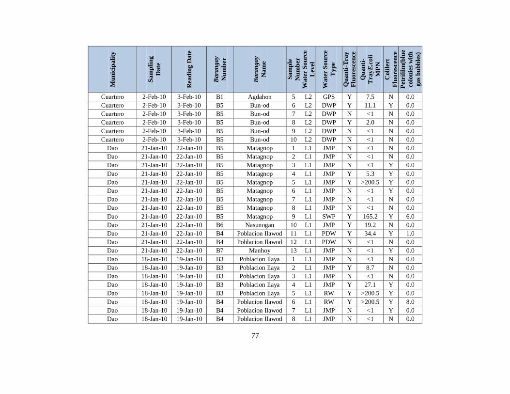
77
Mu
nic
ipali
ty
Sa
mp
lin
g
Da
te
Rea
din
g D
ate
Ba
ran
gay
Nu
mb
er
Ba
ran
gay
Na
me
Sa
mp
le
Nu
mb
er
Wa
ter S
ou
rce
Lev
el
Wa
ter S
ou
rce
Ty
pe
Qu
an
ti-T
ray
Flu
ore
scen
ce
Qu
an
ti-
Tra
yE
.coli
MP
N
Co
lile
rt
Flu
ore
scen
ce
Petr
ifil
m(b
lue
co
lon
ies
wit
h
ga
s b
ub
ble
s)
Cuartero 2-Feb-10 3-Feb-10 B1 Agdahon 5 L2 GPS Y 7.5 N 0.0
Cuartero 2-Feb-10 3-Feb-10 B5 Bun-od 6 L2 DWP Y 11.1 Y 0.0
Cuartero 2-Feb-10 3-Feb-10 B5 Bun-od 7 L2 DWP N <1 N 0.0
Cuartero 2-Feb-10 3-Feb-10 B5 Bun-od 8 L2 DWP Y 2.0 N 0.0
Cuartero 2-Feb-10 3-Feb-10 B5 Bun-od 9 L2 DWP N <1 N 0.0
Cuartero 2-Feb-10 3-Feb-10 B5 Bun-od 10 L2 DWP N <1 N 0.0
Dao 21-Jan-10 22-Jan-10 B5 Matagnop 1 L1 JMP N <1 N 0.0
Dao 21-Jan-10 22-Jan-10 B5 Matagnop 2 L1 JMP N <1 N 0.0
Dao 21-Jan-10 22-Jan-10 B5 Matagnop 3 L1 JMP N <1 Y 0.0
Dao 21-Jan-10 22-Jan-10 B5 Matagnop 4 L1 JMP Y 5.3 Y 0.0
Dao 21-Jan-10 22-Jan-10 B5 Matagnop 5 L1 JMP Y >200.5 Y 0.0
Dao 21-Jan-10 22-Jan-10 B5 Matagnop 6 L1 JMP N <1 Y 0.0
Dao 21-Jan-10 22-Jan-10 B5 Matagnop 7 L1 JMP N <1 N 0.0
Dao 21-Jan-10 22-Jan-10 B5 Matagnop 8 L1 JMP N <1 N 0.0
Dao 21-Jan-10 22-Jan-10 B5 Matagnop 9 L1 SWP Y 165.2 Y 6.0
Dao 21-Jan-10 22-Jan-10 B6 Nasunogan 10 L1 JMP Y 19.2 N 0.0
Dao 21-Jan-10 22-Jan-10 B4 Poblacion Ilawod 11 L1 PDW Y 34.4 Y 1.0
Dao 21-Jan-10 22-Jan-10 B4 Poblacion Ilawod 12 L1 PDW N <1 N 0.0
Dao 21-Jan-10 22-Jan-10 B7 Manhoy 13 L1 JMP N <1 Y 0.0
Dao 18-Jan-10 19-Jan-10 B3 Poblacion Ilaya 1 L1 JMP N <1 N 0.0
Dao 18-Jan-10 19-Jan-10 B3 Poblacion Ilaya 2 L1 JMP Y 8.7 N 0.0
Dao 18-Jan-10 19-Jan-10 B3 Poblacion Ilaya 3 L1 JMP N <1 N 0.0
Dao 18-Jan-10 19-Jan-10 B3 Poblacion Ilaya 4 L1 JMP Y 27.1 Y 0.0
Dao 18-Jan-10 19-Jan-10 B3 Poblacion Ilaya 5 L1 RW Y >200.5 Y 0.0
Dao 18-Jan-10 19-Jan-10 B4 Poblacion Ilawod 6 L1 RW Y >200.5 Y 8.0
Dao 18-Jan-10 19-Jan-10 B4 Poblacion Ilawod 7 L1 JMP N <1 Y 0.0
Dao 18-Jan-10 19-Jan-10 B4 Poblacion Ilawod 8 L1 JMP N <1 N 0.0
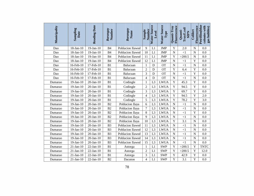
78
Mu
nic
ipali
ty
Sa
mp
lin
g
Da
te
Rea
din
g D
ate
Ba
ran
gay
Nu
mb
er
Ba
ran
gay
Na
me
Sa
mp
le
Nu
mb
er
Wa
ter S
ou
rce
Lev
el
Wa
ter S
ou
rce
Ty
pe
Qu
an
ti-T
ray
Flu
ore
scen
ce
Qu
an
ti-
Tra
yE
.coli
MP
N
Co
lile
rt
Flu
ore
scen
ce
Petr
ifil
m(b
lue
co
lon
ies
wit
h
ga
s b
ub
ble
s)
Dao 18-Jan-10 19-Jan-10 B4 Poblacion Ilawod 9 L1 JMP Y 2.0 N 0.0
Dao 18-Jan-10 19-Jan-10 B4 Poblacion Ilawod 10 L1 JMP N <1 N 0.0
Dao 18-Jan-10 19-Jan-10 B4 Poblacion Ilawod 11 L1 JMP Y >200.5 N 8.0
Dao 18-Jan-10 19-Jan-10 B4 Poblacion Ilawod 12 L1 JMP N <1 Y 0.0
Dao 16-Feb-10 17-Feb-10 B1 Balucuan 1 D OT N <1 N 0.0
Dao 16-Feb-10 17-Feb-10 B1 Balucuan 2 D OT Y 6.4 Y 0.0
Dao 16-Feb-10 17-Feb-10 B1 Balucuan 3 D OT N <1 Y 0.0
Dao 16-Feb-10 17-Feb-10 B1 Balucuan 4 D OT N <1 N 0.0
Dumarao 19-Jan-10 20-Jan-10 B1 Codingle 1 L3 LWUA Y 45.3 Y 0.0
Dumarao 19-Jan-10 20-Jan-10 B1 Codingle 2 L3 LWUA Y 94.5 Y 0.0
Dumarao 19-Jan-10 20-Jan-10 B1 Codingle 3 L3 LWUA Y 69.7 Y 0.0
Dumarao 19-Jan-10 20-Jan-10 B1 Codingle 4 L3 LWUA Y 94.5 Y 2.0
Dumarao 19-Jan-10 20-Jan-10 B1 Codingle 5 L3 LWUA Y 78.2 Y 3.0
Dumarao 19-Jan-10 20-Jan-10 B2 Poblacion Ilaya 6 L3 LWUA N <1 N 0.0
Dumarao 19-Jan-10 20-Jan-10 B2 Poblacion Ilaya 7 L3 LWUA N <1 N 0.0
Dumarao 19-Jan-10 20-Jan-10 B2 Poblacion Ilaya 8 L3 LWUA N <1 Y 0.0
Dumarao 19-Jan-10 20-Jan-10 B2 Poblacion Ilaya 9 L3 LWUA N <1 N 0.0
Dumarao 19-Jan-10 20-Jan-10 B2 Poblacion Ilaya 10 L3 LWUA Y 3.1 N 0.0
Dumarao 19-Jan-10 20-Jan-10 B3 Poblacion Ilawod 11 L3 LWUA N <1 N 0.0
Dumarao 19-Jan-10 20-Jan-10 B3 Poblacion Ilawod 12 L3 LWUA N <1 N 0.0
Dumarao 19-Jan-10 20-Jan-10 B3 Poblacion Ilawod 13 L3 LWUA N <1 N 0.0
Dumarao 19-Jan-10 20-Jan-10 B3 Poblacion Ilawod 14 L3 LWUA N <1 N 0.0
Dumarao 19-Jan-10 20-Jan-10 B3 Poblacion Ilawod 15 L3 LWUA N <1 N 0.0
Dumarao 21-Jan-10 22-Jan-10 B1 Astorga 1 L1 SWP Y >200.5 Y TNTC
Dumarao 21-Jan-10 22-Jan-10 B1 Astorga 2 L1 SWP Y >200.5 Y 12.0
Dumarao 21-Jan-10 22-Jan-10 B1 Astorga 3 L1 SWP Y 42.9 Y 0.0
Dumarao 21-Jan-10 22-Jan-10 B2 Dacuton 4 L1 SWP Y 3.1 Y 0.0
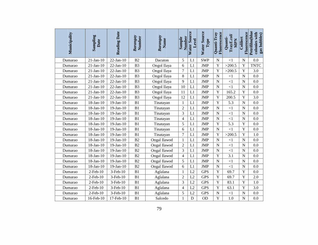
79
Mu
nic
ipali
ty
Sa
mp
lin
g
Da
te
Rea
din
g D
ate
Ba
ran
gay
Nu
mb
er
Ba
ran
gay
Na
me
Sa
mp
le
Nu
mb
er
Wa
ter S
ou
rce
Lev
el
Wa
ter S
ou
rce
Ty
pe
Qu
an
ti-T
ray
Flu
ore
scen
ce
Qu
an
ti-
Tra
yE
.coli
MP
N
Co
lile
rt
Flu
ore
scen
ce
Petr
ifil
m(b
lue
co
lon
ies
wit
h
ga
s b
ub
ble
s)
Dumarao 21-Jan-10 22-Jan-10 B2 Dacuton 5 L1 SWP N <1 N 0.0
Dumarao 21-Jan-10 22-Jan-10 B3 Ongol Ilaya 6 L1 JMP Y >200.5 Y TNTC
Dumarao 21-Jan-10 22-Jan-10 B3 Ongol Ilaya 7 L1 JMP Y >200.5 Y 3.0
Dumarao 21-Jan-10 22-Jan-10 B3 Ongol Ilaya 8 L1 JMP N <1 N 0.0
Dumarao 21-Jan-10 22-Jan-10 B3 Ongol Ilaya 9 L1 JMP N <1 N 0.0
Dumarao 21-Jan-10 22-Jan-10 B3 Ongol Ilaya 10 L1 JMP N <1 N 0.0
Dumarao 21-Jan-10 22-Jan-10 B3 Ongol Ilaya 11 L1 JMP Y 165.2 Y 0.0
Dumarao 21-Jan-10 22-Jan-10 B3 Ongol Ilaya 12 L1 JMP Y 200.5 Y 3.0
Dumarao 18-Jan-10 19-Jan-10 B1 Tinatayan 1 L1 JMP Y 5.3 N 0.0
Dumarao 18-Jan-10 19-Jan-10 B1 Tinatayan 2 L1 JMP N <1 N 0.0
Dumarao 18-Jan-10 19-Jan-10 B1 Tinatayan 3 L1 JMP N <1 N 0.0
Dumarao 18-Jan-10 19-Jan-10 B1 Tinatayan 4 L1 JMP N <1 N 0.0
Dumarao 18-Jan-10 19-Jan-10 B1 Tinatayan 5 L1 JMP Y 5.3 Y 0.0
Dumarao 18-Jan-10 19-Jan-10 B1 Tinatayan 6 L1 JMP N <1 Y 0.0
Dumarao 18-Jan-10 19-Jan-10 B1 Tinatayan 7 L1 JMP Y >200.5 Y 1.0
Dumarao 18-Jan-10 19-Jan-10 B2 Ongal Ilawod 1 L1 JMP N <1 N 0.0
Dumarao 18-Jan-10 19-Jan-10 B2 Ongal Ilawod 2 L1 JMP N <1 N 0.0
Dumarao 18-Jan-10 19-Jan-10 B2 Ongal Ilawod 3 L1 JMP N <1 N 0.0
Dumarao 18-Jan-10 19-Jan-10 B2 Ongal Ilawod 4 L1 JMP Y 3.1 N 0.0
Dumarao 18-Jan-10 19-Jan-10 B2 Ongal Ilawod 5 L1 JMP N <1 N 0.0
Dumarao 18-Jan-10 19-Jan-10 B2 Ongal Ilawod 6 L1 JMP N <1 N 0.0
Dumarao 2-Feb-10 3-Feb-10 B1 Aglalana 1 L2 GPS Y 69.7 Y 0.0
Dumarao 2-Feb-10 3-Feb-10 B1 Aglalana 2 L2 GPS Y 69.7 Y 2.0
Dumarao 2-Feb-10 3-Feb-10 B1 Aglalana 3 L2 GPS Y 83.1 Y 1.0
Dumarao 2-Feb-10 3-Feb-10 B1 Aglalana 4 L2 GPS Y 63.1 Y 3.0
Dumarao 2-Feb-10 3-Feb-10 B1 Aglalana 5 L2 GPS N <1 N 0.0
Dumarao 16-Feb-10 17-Feb-10 B1 Salcedo 1 D OD Y 1.0 N 0.0
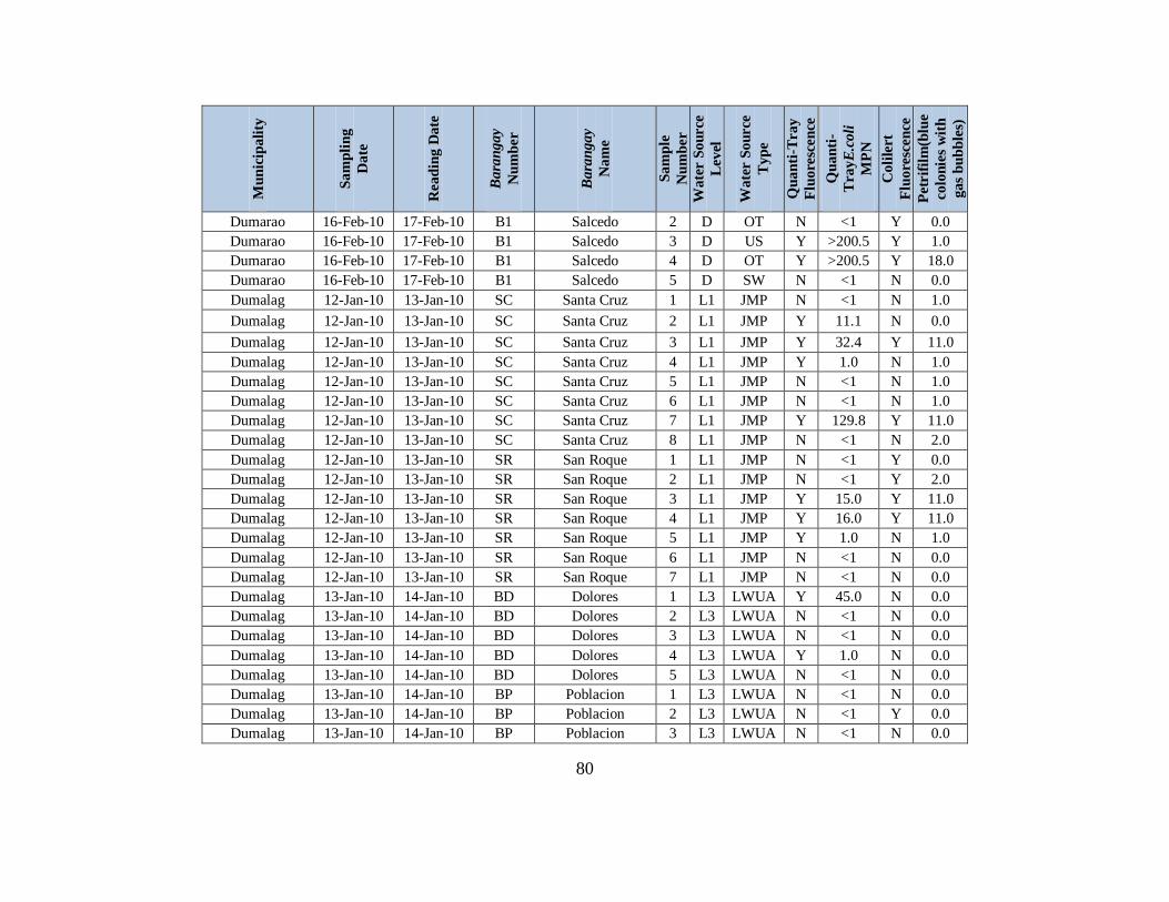
80
Mu
nic
ipali
ty
Sa
mp
lin
g
Da
te
Rea
din
g D
ate
Ba
ran
gay
Nu
mb
er
Ba
ran
gay
Na
me
Sa
mp
le
Nu
mb
er
Wa
ter S
ou
rce
Lev
el
Wa
ter S
ou
rce
Ty
pe
Qu
an
ti-T
ray
Flu
ore
scen
ce
Qu
an
ti-
Tra
yE
.coli
MP
N
Co
lile
rt
Flu
ore
scen
ce
Petr
ifil
m(b
lue
co
lon
ies
wit
h
ga
s b
ub
ble
s)
Dumarao 16-Feb-10 17-Feb-10 B1 Salcedo 2 D OT N <1 Y 0.0
Dumarao 16-Feb-10 17-Feb-10 B1 Salcedo 3 D US Y >200.5 Y 1.0
Dumarao 16-Feb-10 17-Feb-10 B1 Salcedo 4 D OT Y >200.5 Y 18.0
Dumarao 16-Feb-10 17-Feb-10 B1 Salcedo 5 D SW N <1 N 0.0
Dumalag 12-Jan-10 13-Jan-10 SC Santa Cruz 1 L1 JMP N <1 N 1.0
Dumalag 12-Jan-10 13-Jan-10 SC Santa Cruz 2 L1 JMP Y 11.1 N 0.0
Dumalag 12-Jan-10 13-Jan-10 SC Santa Cruz 3 L1 JMP Y 32.4 Y 11.0
Dumalag 12-Jan-10 13-Jan-10 SC Santa Cruz 4 L1 JMP Y 1.0 N 1.0
Dumalag 12-Jan-10 13-Jan-10 SC Santa Cruz 5 L1 JMP N <1 N 1.0
Dumalag 12-Jan-10 13-Jan-10 SC Santa Cruz 6 L1 JMP N <1 N 1.0
Dumalag 12-Jan-10 13-Jan-10 SC Santa Cruz 7 L1 JMP Y 129.8 Y 11.0
Dumalag 12-Jan-10 13-Jan-10 SC Santa Cruz 8 L1 JMP N <1 N 2.0
Dumalag 12-Jan-10 13-Jan-10 SR San Roque 1 L1 JMP N <1 Y 0.0
Dumalag 12-Jan-10 13-Jan-10 SR San Roque 2 L1 JMP N <1 Y 2.0
Dumalag 12-Jan-10 13-Jan-10 SR San Roque 3 L1 JMP Y 15.0 Y 11.0
Dumalag 12-Jan-10 13-Jan-10 SR San Roque 4 L1 JMP Y 16.0 Y 11.0
Dumalag 12-Jan-10 13-Jan-10 SR San Roque 5 L1 JMP Y 1.0 N 1.0
Dumalag 12-Jan-10 13-Jan-10 SR San Roque 6 L1 JMP N <1 N 0.0
Dumalag 12-Jan-10 13-Jan-10 SR San Roque 7 L1 JMP N <1 N 0.0
Dumalag 13-Jan-10 14-Jan-10 BD Dolores 1 L3 LWUA Y 45.0 N 0.0
Dumalag 13-Jan-10 14-Jan-10 BD Dolores 2 L3 LWUA N <1 N 0.0
Dumalag 13-Jan-10 14-Jan-10 BD Dolores 3 L3 LWUA N <1 N 0.0
Dumalag 13-Jan-10 14-Jan-10 BD Dolores 4 L3 LWUA Y 1.0 N 0.0
Dumalag 13-Jan-10 14-Jan-10 BD Dolores 5 L3 LWUA N <1 N 0.0
Dumalag 13-Jan-10 14-Jan-10 BP Poblacion 1 L3 LWUA N <1 N 0.0
Dumalag 13-Jan-10 14-Jan-10 BP Poblacion 2 L3 LWUA N <1 Y 0.0
Dumalag 13-Jan-10 14-Jan-10 BP Poblacion 3 L3 LWUA N <1 N 0.0

81
Mu
nic
ipali
ty
Sa
mp
lin
g
Da
te
Rea
din
g D
ate
Ba
ran
gay
Nu
mb
er
Ba
ran
gay
Na
me
Sa
mp
le
Nu
mb
er
Wa
ter S
ou
rce
Lev
el
Wa
ter S
ou
rce
Ty
pe
Qu
an
ti-T
ray
Flu
ore
scen
ce
Qu
an
ti-
Tra
yE
.coli
MP
N
Co
lile
rt
Flu
ore
scen
ce
Petr
ifil
m(b
lue
co
lon
ies
wit
h
ga
s b
ub
ble
s)
Dumalag 13-Jan-10 14-Jan-10 BP Poblacion 4 L3 LWUA N <1 N 2.0
Dumalag 13-Jan-10 14-Jan-10 BP Poblacion 5 L3 LWUA N <1 N 0.0
Dumalag 13-Jan-10 14-Jan-10 BSA San Angel 1 D OD Y >200.5 Y 6.0
Dumalag 13-Jan-10 14-Jan-10 BSA San Angel 2 D OD Y 165.2 Y 0.0
Dumalag 13-Jan-10 14-Jan-10 BSA San Angel 3 D OD Y >200.5 Y 7.0
Dumalag 13-Jan-10 14-Jan-10 BSA San Angel 4 D OD Y >200.5 Y TNTC
Dumalag 13-Jan-10 14-Jan-10 BC Concepcion 1 L1 PS N <1 N 0.0
Tapaz 20-Jan-10 21-Jan-10 B6 San Julian 1 L2 DWP Y 8.7 N 0.0
Tapaz 20-Jan-10 21-Jan-10 B6 San Julian 2 L2 DWP N <1 N 0.0
Tapaz 20-Jan-10 21-Jan-10 B6 San Julian 3 L2 DWP N <1 N 0.0
Tapaz 20-Jan-10 21-Jan-10 B6 San Julian 4 L2 DWP Y 1.0 N 0.0
Tapaz 20-Jan-10 21-Jan-10 B6 San Julian 5 L2 DWP N <1 N 0.0
Tapaz 20-Jan-10 21-Jan-10 B7 San Nicolas 1 L2 GPS N <1 N 0.0
Tapaz 20-Jan-10 21-Jan-10 B7 San Nicolas 2 L2 GPS N <1 N 0.0
Tapaz 20-Jan-10 21-Jan-10 B7 San Nicolas 3 L2 GPS N <1 N 0.0
Tapaz 20-Jan-10 21-Jan-10 B7 San Nicolas 4 L2 GPS N <1 N 0.0
Tapaz 20-Jan-10 21-Jan-10 B7 San Nicolas 5 L2 GPS Y 2.0 N 0.0
Tapaz 12-Jan-10 13-Jan-10 B1 Salong 1 L1 PDW Y >200.5 Y 5.0
Tapaz 12-Jan-10 13-Jan-10 B1 Salong 6 L1 JMP Y <1 N 0.0
Tapaz 12-Jan-10 13-Jan-10 B1 Salong 11 L1 JMP Y 9.9 Y 0.0
Tapaz 12-Jan-10 13-Jan-10 B1 Salong 12 L1 JMP Y 2.0 N 0.0
Tapaz 12-Jan-10 13-Jan-10 B1 Salong 13 L1 DWP Y 1.0 N 0.0
Tapaz 12-Jan-10 13-Jan-10 B2 Carida 3 L1 JMP Y 165.2 Y 1.0
Tapaz 12-Jan-10 13-Jan-10 B2 Carida 4 L1 JMP Y 2.0 N 0.0
Tapaz 12-Jan-10 13-Jan-10 B2 Carida 5 L1 JMP Y >200.5 Y 4.0
Tapaz 12-Jan-10 13-Jan-10 B2 Carida 7 L1 JMP Y 5.3 Y 2.0
Tapaz 12-Jan-10 13-Jan-10 B2 Carida 8 L1 DWP Y 17.8 Y 1.0
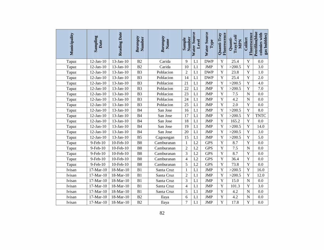
82
Mu
nic
ipali
ty
Sa
mp
lin
g
Da
te
Rea
din
g D
ate
Ba
ran
gay
Nu
mb
er
Ba
ran
gay
Na
me
Sa
mp
le
Nu
mb
er
Wa
ter S
ou
rce
Lev
el
Wa
ter S
ou
rce
Ty
pe
Qu
an
ti-T
ray
Flu
ore
scen
ce
Qu
an
ti-
Tra
yE
.coli
MP
N
Co
lile
rt
Flu
ore
scen
ce
Petr
ifil
m(b
lue
co
lon
ies
wit
h
ga
s b
ub
ble
s)
Tapaz 12-Jan-10 13-Jan-10 B2 Carida 9 L1 DWP Y 25.4 Y 0.0
Tapaz 12-Jan-10 13-Jan-10 B2 Carida 10 L1 JMP Y >200.5 Y 3.0
Tapaz 12-Jan-10 13-Jan-10 B3 Poblacion 2 L1 DWP Y 23.8 Y 1.0
Tapaz 12-Jan-10 13-Jan-10 B3 Poblacion 14 L1 DWP Y 25.4 Y 2.0
Tapaz 12-Jan-10 13-Jan-10 B3 Poblacion 21 L1 JMP Y >200.5 Y 4.0
Tapaz 12-Jan-10 13-Jan-10 B3 Poblacion 22 L1 JMP Y >200.5 Y 7.0
Tapaz 12-Jan-10 13-Jan-10 B3 Poblacion 23 L1 JMP Y 7.5 N 0.0
Tapaz 12-Jan-10 13-Jan-10 B3 Poblacion 24 L1 JMP Y 4.2 N 0.0
Tapaz 12-Jan-10 13-Jan-10 B3 Poblacion 25 L1 JMP Y 2.0 Y 0.0
Tapaz 12-Jan-10 13-Jan-10 B4 San Jose 16 L1 JMP Y >200.5 Y 8.0
Tapaz 12-Jan-10 13-Jan-10 B4 San Jose 17 L1 JMP Y >200.5 Y TNTC
Tapaz 12-Jan-10 13-Jan-10 B4 San Jose 18 L1 JMP Y 165.2 Y 0.0
Tapaz 12-Jan-10 13-Jan-10 B4 San Jose 19 L1 JMP Y >200.5 Y 14.0
Tapaz 12-Jan-10 13-Jan-10 B4 San Jose 20 L1 JMP Y >200.5 Y 3.0
Tapaz 12-Jan-10 13-Jan-10 B5 Cagoungan 15 L1 JMP Y >200.5 Y 5.0
Tapaz 9-Feb-10 10-Feb-10 B8 Camburanan 1 L2 GPS Y 8.7 Y 0.0
Tapaz 9-Feb-10 10-Feb-10 B8 Camburanan 2 L2 GPS Y 7.5 N 0.0
Tapaz 9-Feb-10 10-Feb-10 B8 Camburanan 3 L2 GPS Y 8.7 Y 0.0
Tapaz 9-Feb-10 10-Feb-10 B8 Camburanan 4 L2 GPS Y 36.4 Y 0.0
Tapaz 9-Feb-10 10-Feb-10 B8 Camburanan 5 L2 GPS Y 73.8 Y 0.0
Ivisan 17-Mar-10 18-Mar-10 B1 Santa Cruz 1 L1 JMP Y >200.5 Y 16.0
Ivisan 17-Mar-10 18-Mar-10 B1 Santa Cruz 2 L1 JMP Y >200.5 Y 12.0
Ivisan 17-Mar-10 18-Mar-10 B1 Santa Cruz 3 L1 JMP Y 15.0 N 0.0
Ivisan 17-Mar-10 18-Mar-10 B1 Santa Cruz 4 L1 JMP Y 101.3 Y 3.0
Ivisan 17-Mar-10 18-Mar-10 B1 Santa Cruz 5 L1 JMP Y 4.2 N 0.0
Ivisan 17-Mar-10 18-Mar-10 B2 Ilaya 6 L1 JMP Y 4.2 N 0.0
Ivisan 17-Mar-10 18-Mar-10 B2 Ilaya 7 L1 JMP Y 17.8 Y 0.0
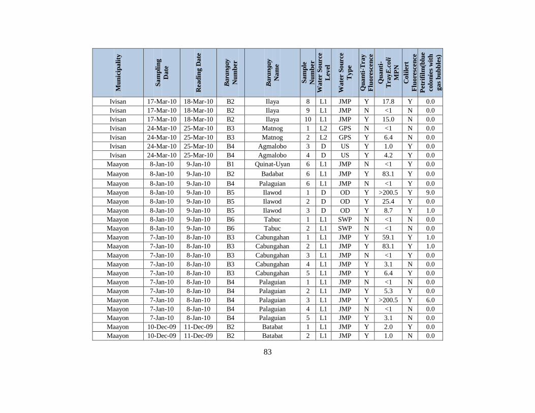
83
Mu
nic
ipali
ty
Sa
mp
lin
g
Da
te
Rea
din
g D
ate
Ba
ran
gay
Nu
mb
er
Ba
ran
gay
Na
me
Sa
mp
le
Nu
mb
er
Wa
ter S
ou
rce
Lev
el
Wa
ter S
ou
rce
Ty
pe
Qu
an
ti-T
ray
Flu
ore
scen
ce
Qu
an
ti-
Tra
yE
.coli
MP
N
Co
lile
rt
Flu
ore
scen
ce
Petr
ifil
m(b
lue
co
lon
ies
wit
h
ga
s b
ub
ble
s)
Ivisan 17-Mar-10 18-Mar-10 B2 Ilaya 8 L1 JMP Y 17.8 Y 0.0
Ivisan 17-Mar-10 18-Mar-10 B2 Ilaya 9 L1 JMP N <1 N 0.0
Ivisan 17-Mar-10 18-Mar-10 B2 Ilaya 10 L1 JMP Y 15.0 N 0.0
Ivisan 24-Mar-10 25-Mar-10 B3 Matnog 1 L2 GPS N <1 N 0.0
Ivisan 24-Mar-10 25-Mar-10 B3 Matnog 2 L2 GPS Y 6.4 N 0.0
Ivisan 24-Mar-10 25-Mar-10 B4 Agmalobo 3 D US Y 1.0 Y 0.0
Ivisan 24-Mar-10 25-Mar-10 B4 Agmalobo 4 D US Y 4.2 Y 0.0
Maayon 8-Jan-10 9-Jan-10 B1 Quinat-Uyan 6 L1 JMP N <1 Y 0.0
Maayon 8-Jan-10 9-Jan-10 B2 Badabat 6 L1 JMP Y 83.1 Y 0.0
Maayon 8-Jan-10 9-Jan-10 B4 Palaguian 6 L1 JMP N <1 Y 0.0
Maayon 8-Jan-10 9-Jan-10 B5 Ilawod 1 D OD Y >200.5 Y 9.0
Maayon 8-Jan-10 9-Jan-10 B5 Ilawod 2 D OD Y 25.4 Y 0.0
Maayon 8-Jan-10 9-Jan-10 B5 Ilawod 3 D OD Y 8.7 Y 1.0
Maayon 8-Jan-10 9-Jan-10 B6 Tabuc 1 L1 SWP N <1 N 0.0
Maayon 8-Jan-10 9-Jan-10 B6 Tabuc 2 L1 SWP N <1 N 0.0
Maayon 7-Jan-10 8-Jan-10 B3 Cabungahan 1 L1 JMP Y 59.1 Y 1.0
Maayon 7-Jan-10 8-Jan-10 B3 Cabungahan 2 L1 JMP Y 83.1 Y 1.0
Maayon 7-Jan-10 8-Jan-10 B3 Cabungahan 3 L1 JMP N <1 Y 0.0
Maayon 7-Jan-10 8-Jan-10 B3 Cabungahan 4 L1 JMP Y 3.1 N 0.0
Maayon 7-Jan-10 8-Jan-10 B3 Cabungahan 5 L1 JMP Y 6.4 Y 0.0
Maayon 7-Jan-10 8-Jan-10 B4 Palaguian 1 L1 JMP N <1 N 0.0
Maayon 7-Jan-10 8-Jan-10 B4 Palaguian 2 L1 JMP Y 5.3 Y 0.0
Maayon 7-Jan-10 8-Jan-10 B4 Palaguian 3 L1 JMP Y >200.5 Y 6.0
Maayon 7-Jan-10 8-Jan-10 B4 Palaguian 4 L1 JMP N <1 N 0.0
Maayon 7-Jan-10 8-Jan-10 B4 Palaguian 5 L1 JMP Y 3.1 N 0.0
Maayon 10-Dec-09 11-Dec-09 B2 Batabat 1 L1 JMP Y 2.0 Y 0.0
Maayon 10-Dec-09 11-Dec-09 B2 Batabat 2 L1 JMP Y 1.0 N 0.0
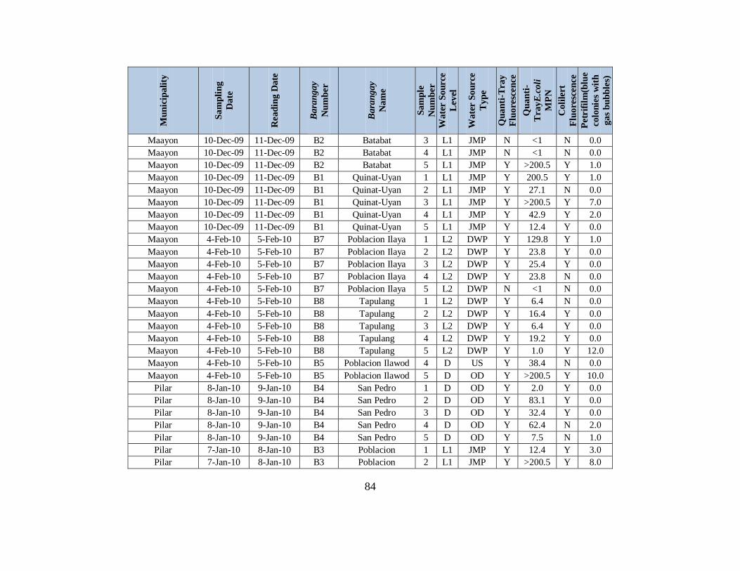
84
Mu
nic
ipali
ty
Sa
mp
lin
g
Da
te
Rea
din
g D
ate
Ba
ran
gay
Nu
mb
er
Ba
ran
gay
Na
me
Sa
mp
le
Nu
mb
er
Wa
ter S
ou
rce
Lev
el
Wa
ter S
ou
rce
Ty
pe
Qu
an
ti-T
ray
Flu
ore
scen
ce
Qu
an
ti-
Tra
yE
.coli
MP
N
Co
lile
rt
Flu
ore
scen
ce
Petr
ifil
m(b
lue
co
lon
ies
wit
h
ga
s b
ub
ble
s)
Maayon 10-Dec-09 11-Dec-09 B2 Batabat 3 L1 JMP N <1 N 0.0
Maayon 10-Dec-09 11-Dec-09 B2 Batabat 4 L1 JMP N <1 N 0.0
Maayon 10-Dec-09 11-Dec-09 B2 Batabat 5 L1 JMP Y >200.5 Y 1.0
Maayon 10-Dec-09 11-Dec-09 B1 Quinat-Uyan 1 L1 JMP Y 200.5 Y 1.0
Maayon 10-Dec-09 11-Dec-09 B1 Quinat-Uyan 2 L1 JMP Y 27.1 N 0.0
Maayon 10-Dec-09 11-Dec-09 B1 Quinat-Uyan 3 L1 JMP Y >200.5 Y 7.0
Maayon 10-Dec-09 11-Dec-09 B1 Quinat-Uyan 4 L1 JMP Y 42.9 Y 2.0
Maayon 10-Dec-09 11-Dec-09 B1 Quinat-Uyan 5 L1 JMP Y 12.4 Y 0.0
Maayon 4-Feb-10 5-Feb-10 B7 Poblacion Ilaya 1 L2 DWP Y 129.8 Y 1.0
Maayon 4-Feb-10 5-Feb-10 B7 Poblacion Ilaya 2 L2 DWP Y 23.8 Y 0.0
Maayon 4-Feb-10 5-Feb-10 B7 Poblacion Ilaya 3 L2 DWP Y 25.4 Y 0.0
Maayon 4-Feb-10 5-Feb-10 B7 Poblacion Ilaya 4 L2 DWP Y 23.8 N 0.0
Maayon 4-Feb-10 5-Feb-10 B7 Poblacion Ilaya 5 L2 DWP N <1 N 0.0
Maayon 4-Feb-10 5-Feb-10 B8 Tapulang 1 L2 DWP Y 6.4 N 0.0
Maayon 4-Feb-10 5-Feb-10 B8 Tapulang 2 L2 DWP Y 16.4 Y 0.0
Maayon 4-Feb-10 5-Feb-10 B8 Tapulang 3 L2 DWP Y 6.4 Y 0.0
Maayon 4-Feb-10 5-Feb-10 B8 Tapulang 4 L2 DWP Y 19.2 Y 0.0
Maayon 4-Feb-10 5-Feb-10 B8 Tapulang 5 L2 DWP Y 1.0 Y 12.0
Maayon 4-Feb-10 5-Feb-10 B5 Poblacion Ilawod 4 D US Y 38.4 N 0.0
Maayon 4-Feb-10 5-Feb-10 B5 Poblacion Ilawod 5 D OD Y >200.5 Y 10.0
Pilar 8-Jan-10 9-Jan-10 B4 San Pedro 1 D OD Y 2.0 Y 0.0
Pilar 8-Jan-10 9-Jan-10 B4 San Pedro 2 D OD Y 83.1 Y 0.0
Pilar 8-Jan-10 9-Jan-10 B4 San Pedro 3 D OD Y 32.4 Y 0.0
Pilar 8-Jan-10 9-Jan-10 B4 San Pedro 4 D OD Y 62.4 N 2.0
Pilar 8-Jan-10 9-Jan-10 B4 San Pedro 5 D OD Y 7.5 N 1.0
Pilar 7-Jan-10 8-Jan-10 B3 Poblacion 1 L1 JMP Y 12.4 Y 3.0
Pilar 7-Jan-10 8-Jan-10 B3 Poblacion 2 L1 JMP Y >200.5 Y 8.0
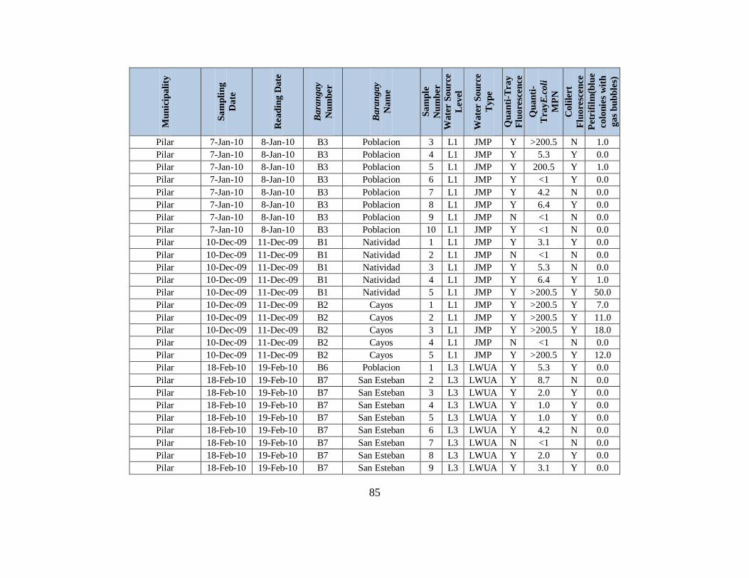
85
Mu
nic
ipali
ty
Sa
mp
lin
g
Da
te
Rea
din
g D
ate
Ba
ran
gay
Nu
mb
er
Ba
ran
gay
Na
me
Sa
mp
le
Nu
mb
er
Wa
ter S
ou
rce
Lev
el
Wa
ter S
ou
rce
Ty
pe
Qu
an
ti-T
ray
Flu
ore
scen
ce
Qu
an
ti-
Tra
yE
.coli
MP
N
Co
lile
rt
Flu
ore
scen
ce
Petr
ifil
m(b
lue
co
lon
ies
wit
h
ga
s b
ub
ble
s)
Pilar 7-Jan-10 8-Jan-10 B3 Poblacion 3 L1 JMP Y >200.5 N 1.0
Pilar 7-Jan-10 8-Jan-10 B3 Poblacion 4 L1 JMP Y 5.3 Y 0.0
Pilar 7-Jan-10 8-Jan-10 B3 Poblacion 5 L1 JMP Y 200.5 Y 1.0
Pilar 7-Jan-10 8-Jan-10 B3 Poblacion 6 L1 JMP Y <1 Y 0.0
Pilar 7-Jan-10 8-Jan-10 B3 Poblacion 7 L1 JMP Y 4.2 N 0.0
Pilar 7-Jan-10 8-Jan-10 B3 Poblacion 8 L1 JMP Y 6.4 Y 0.0
Pilar 7-Jan-10 8-Jan-10 B3 Poblacion 9 L1 JMP N <1 N 0.0
Pilar 7-Jan-10 8-Jan-10 B3 Poblacion 10 L1 JMP Y <1 N 0.0
Pilar 10-Dec-09 11-Dec-09 B1 Natividad 1 L1 JMP Y 3.1 Y 0.0
Pilar 10-Dec-09 11-Dec-09 B1 Natividad 2 L1 JMP N <1 N 0.0
Pilar 10-Dec-09 11-Dec-09 B1 Natividad 3 L1 JMP Y 5.3 N 0.0
Pilar 10-Dec-09 11-Dec-09 B1 Natividad 4 L1 JMP Y 6.4 Y 1.0
Pilar 10-Dec-09 11-Dec-09 B1 Natividad 5 L1 JMP Y >200.5 Y 50.0
Pilar 10-Dec-09 11-Dec-09 B2 Cayos 1 L1 JMP Y >200.5 Y 7.0
Pilar 10-Dec-09 11-Dec-09 B2 Cayos 2 L1 JMP Y >200.5 Y 11.0
Pilar 10-Dec-09 11-Dec-09 B2 Cayos 3 L1 JMP Y >200.5 Y 18.0
Pilar 10-Dec-09 11-Dec-09 B2 Cayos 4 L1 JMP N <1 N 0.0
Pilar 10-Dec-09 11-Dec-09 B2 Cayos 5 L1 JMP Y >200.5 Y 12.0
Pilar 18-Feb-10 19-Feb-10 B6 Poblacion 1 L3 LWUA Y 5.3 Y 0.0
Pilar 18-Feb-10 19-Feb-10 B7 San Esteban 2 L3 LWUA Y 8.7 N 0.0
Pilar 18-Feb-10 19-Feb-10 B7 San Esteban 3 L3 LWUA Y 2.0 Y 0.0
Pilar 18-Feb-10 19-Feb-10 B7 San Esteban 4 L3 LWUA Y 1.0 Y 0.0
Pilar 18-Feb-10 19-Feb-10 B7 San Esteban 5 L3 LWUA Y 1.0 Y 0.0
Pilar 18-Feb-10 19-Feb-10 B7 San Esteban 6 L3 LWUA Y 4.2 N 0.0
Pilar 18-Feb-10 19-Feb-10 B7 San Esteban 7 L3 LWUA N <1 N 0.0
Pilar 18-Feb-10 19-Feb-10 B7 San Esteban 8 L3 LWUA Y 2.0 Y 0.0
Pilar 18-Feb-10 19-Feb-10 B7 San Esteban 9 L3 LWUA Y 3.1 Y 0.0
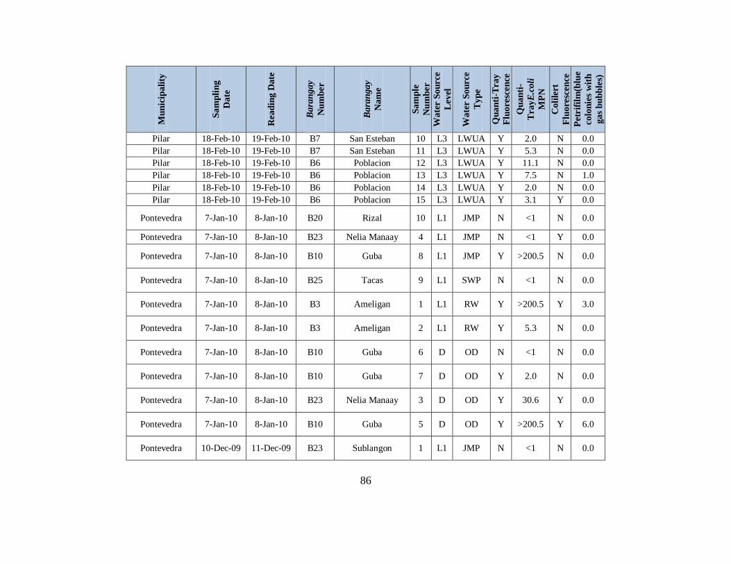
86
Mu
nic
ipali
ty
Sa
mp
lin
g
Da
te
Rea
din
g D
ate
Ba
ran
gay
Nu
mb
er
Ba
ran
gay
Na
me
Sa
mp
le
Nu
mb
er
Wa
ter S
ou
rce
Lev
el
Wa
ter S
ou
rce
Ty
pe
Qu
an
ti-T
ray
Flu
ore
scen
ce
Qu
an
ti-
Tra
yE
.coli
MP
N
Co
lile
rt
Flu
ore
scen
ce
Petr
ifil
m(b
lue
co
lon
ies
wit
h
ga
s b
ub
ble
s)
Pilar 18-Feb-10 19-Feb-10 B7 San Esteban 10 L3 LWUA Y 2.0 N 0.0
Pilar 18-Feb-10 19-Feb-10 B7 San Esteban 11 L3 LWUA Y 5.3 N 0.0
Pilar 18-Feb-10 19-Feb-10 B6 Poblacion 12 L3 LWUA Y 11.1 N 0.0
Pilar 18-Feb-10 19-Feb-10 B6 Poblacion 13 L3 LWUA Y 7.5 N 1.0
Pilar 18-Feb-10 19-Feb-10 B6 Poblacion 14 L3 LWUA Y 2.0 N 0.0
Pilar 18-Feb-10 19-Feb-10 B6 Poblacion 15 L3 LWUA Y 3.1 Y 0.0
Pontevedra 7-Jan-10 8-Jan-10 B20 Rizal 10 L1 JMP N <1 N 0.0
Pontevedra 7-Jan-10 8-Jan-10 B23 Nelia Manaay 4 L1 JMP N <1 Y 0.0
Pontevedra 7-Jan-10 8-Jan-10 B10 Guba 8 L1 JMP Y >200.5 N 0.0
Pontevedra 7-Jan-10 8-Jan-10 B25 Tacas 9 L1 SWP N <1 N 0.0
Pontevedra 7-Jan-10 8-Jan-10 B3 Ameligan 1 L1 RW Y >200.5 Y 3.0
Pontevedra 7-Jan-10 8-Jan-10 B3 Ameligan 2 L1 RW Y 5.3 N 0.0
Pontevedra 7-Jan-10 8-Jan-10 B10 Guba 6 D OD N <1 N 0.0
Pontevedra 7-Jan-10 8-Jan-10 B10 Guba 7 D OD Y 2.0 N 0.0
Pontevedra 7-Jan-10 8-Jan-10 B23 Nelia Manaay 3 D OD Y 30.6 Y 0.0
Pontevedra 7-Jan-10 8-Jan-10 B10 Guba 5 D OD Y >200.5 Y 6.0
Pontevedra 10-Dec-09 11-Dec-09 B23 Sublangon 1 L1 JMP N <1 N 0.0
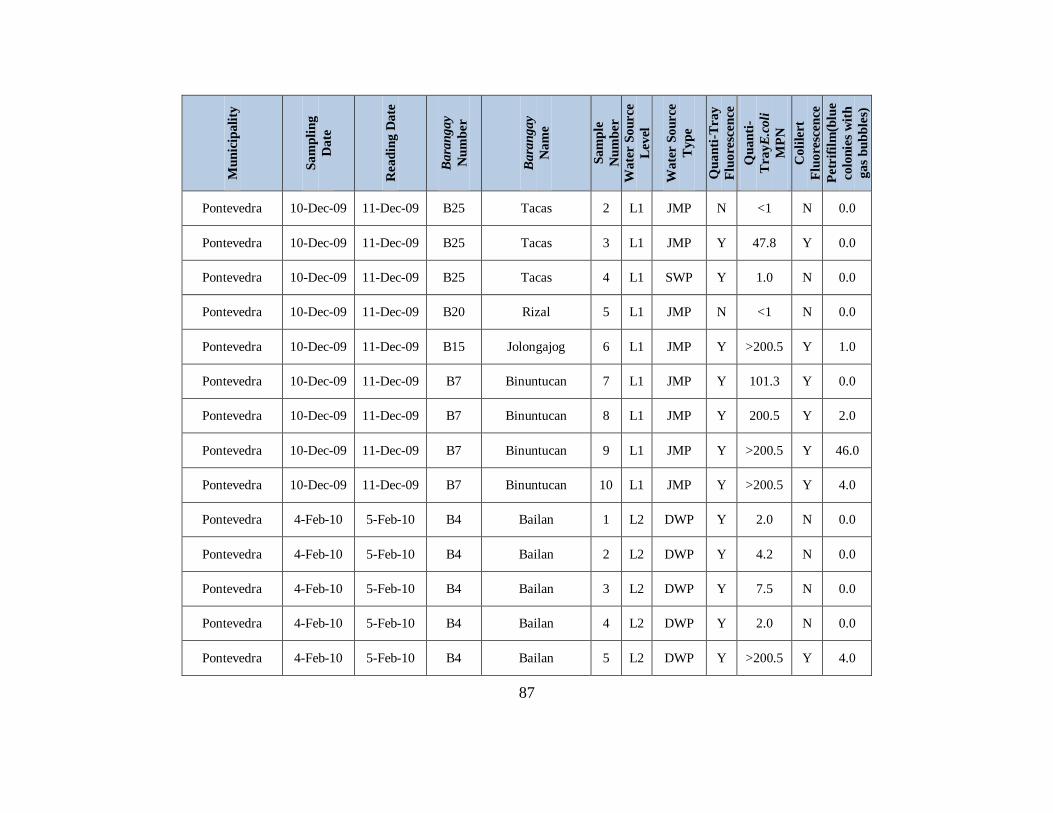
87
Mu
nic
ipali
ty
Sa
mp
lin
g
Da
te
Rea
din
g D
ate
Ba
ran
gay
Nu
mb
er
Ba
ran
gay
Na
me
Sa
mp
le
Nu
mb
er
Wa
ter S
ou
rce
Lev
el
Wa
ter S
ou
rce
Ty
pe
Qu
an
ti-T
ray
Flu
ore
scen
ce
Qu
an
ti-
Tra
yE
.coli
MP
N
Co
lile
rt
Flu
ore
scen
ce
Petr
ifil
m(b
lue
co
lon
ies
wit
h
ga
s b
ub
ble
s)
Pontevedra 10-Dec-09 11-Dec-09 B25 Tacas 2 L1 JMP N <1 N 0.0
Pontevedra 10-Dec-09 11-Dec-09 B25 Tacas 3 L1 JMP Y 47.8 Y 0.0
Pontevedra 10-Dec-09 11-Dec-09 B25 Tacas 4 L1 SWP Y 1.0 N 0.0
Pontevedra 10-Dec-09 11-Dec-09 B20 Rizal 5 L1 JMP N <1 N 0.0
Pontevedra 10-Dec-09 11-Dec-09 B15 Jolongajog 6 L1 JMP Y >200.5 Y 1.0
Pontevedra 10-Dec-09 11-Dec-09 B7 Binuntucan 7 L1 JMP Y 101.3 Y 0.0
Pontevedra 10-Dec-09 11-Dec-09 B7 Binuntucan 8 L1 JMP Y 200.5 Y 2.0
Pontevedra 10-Dec-09 11-Dec-09 B7 Binuntucan 9 L1 JMP Y >200.5 Y 46.0
Pontevedra 10-Dec-09 11-Dec-09 B7 Binuntucan 10 L1 JMP Y >200.5 Y 4.0
Pontevedra 4-Feb-10 5-Feb-10 B4 Bailan 1 L2 DWP Y 2.0 N 0.0
Pontevedra 4-Feb-10 5-Feb-10 B4 Bailan 2 L2 DWP Y 4.2 N 0.0
Pontevedra 4-Feb-10 5-Feb-10 B4 Bailan 3 L2 DWP Y 7.5 N 0.0
Pontevedra 4-Feb-10 5-Feb-10 B4 Bailan 4 L2 DWP Y 2.0 N 0.0
Pontevedra 4-Feb-10 5-Feb-10 B4 Bailan 5 L2 DWP Y >200.5 Y 4.0
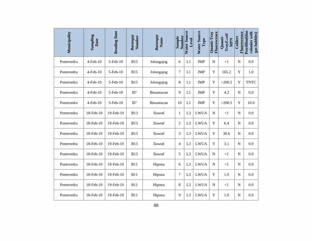
88
Mu
nic
ipali
ty
Sa
mp
lin
g
Da
te
Rea
din
g D
ate
Ba
ran
gay
Nu
mb
er
Ba
ran
gay
Na
me
Sa
mp
le
Nu
mb
er
Wa
ter S
ou
rce
Lev
el
Wa
ter S
ou
rce
Ty
pe
Qu
an
ti-T
ray
Flu
ore
scen
ce
Qu
an
ti-
Tra
yE
.coli
MP
N
Co
lile
rt
Flu
ore
scen
ce
Petr
ifil
m(b
lue
co
lon
ies
wit
h
ga
s b
ub
ble
s)
Pontevedra 4-Feb-10 5-Feb-10 B15 Jolongajog 6 L1 JMP N <1 N 0.0
Pontevedra 4-Feb-10 5-Feb-10 B15 Jolongajog 7 L1 JMP Y 165.2 Y 1.0
Pontevedra 4-Feb-10 5-Feb-10 B15 Jolongajog 8 L1 JMP Y >200.5 Y TNTC
Pontevedra 4-Feb-10 5-Feb-10 B7 Binuntucan 9 L1 JMP Y 4.2 N 0.0
Pontevedra 4-Feb-10 5-Feb-10 B7 Binuntucan 10 L1 JMP Y >200.5 Y 10.0
Pontevedra 18-Feb-10 19-Feb-10 B13 Ilawod 1 L3 LWUA N <1 N 0.0
Pontevedra 18-Feb-10 19-Feb-10 B13 Ilawod 2 L3 LWUA Y 6.4 N 0.0
Pontevedra 18-Feb-10 19-Feb-10 B13 Ilawod 3 L3 LWUA Y 30.6 N 0.0
Pontevedra 18-Feb-10 19-Feb-10 B13 Ilawod 4 L3 LWUA Y 3.1 N 0.0
Pontevedra 18-Feb-10 19-Feb-10 B13 Ilawod 5 L3 LWUA N <1 N 0.0
Pontevedra 18-Feb-10 19-Feb-10 B11 Hipona 6 L3 LWUA N <1 N 0.0
Pontevedra 18-Feb-10 19-Feb-10 B11 Hipona 7 L3 LWUA Y 1.0 N 0.0
Pontevedra 18-Feb-10 19-Feb-10 B11 Hipona 8 L3 LWUA N <1 N 0.0
Pontevedra 18-Feb-10 19-Feb-10 B11 Hipona 9 L3 LWUA Y 1.0 N 0.0
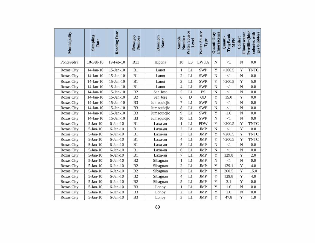
89
Mu
nic
ipali
ty
Sa
mp
lin
g
Da
te
Rea
din
g D
ate
Ba
ran
gay
Nu
mb
er
Ba
ran
gay
Na
me
Sa
mp
le
Nu
mb
er
Wa
ter S
ou
rce
Lev
el
Wa
ter S
ou
rce
Ty
pe
Qu
an
ti-T
ray
Flu
ore
scen
ce
Qu
an
ti-
Tra
yE
.coli
MP
N
Co
lile
rt
Flu
ore
scen
ce
Petr
ifil
m(b
lue
co
lon
ies
wit
h
ga
s b
ub
ble
s)
Pontevedra 18-Feb-10 19-Feb-10 B11 Hipona 10 L3 LWUA N <1 N 0.0
Roxas City 14-Jan-10 15-Jan-10 B1 Lanot 1 L1 SWP Y >200.5 Y TNTC
Roxas City 14-Jan-10 15-Jan-10 B1 Lanot 2 L1 SWP N <1 N 0.0
Roxas City 14-Jan-10 15-Jan-10 B1 Lanot 3 L1 SWP Y >200.5 Y 5.0
Roxas City 14-Jan-10 15-Jan-10 B1 Lanot 4 L1 SWP N <1 N 0.0
Roxas City 14-Jan-10 15-Jan-10 B2 San Jose 5 L1 PS N <1 N 0.0
Roxas City 14-Jan-10 15-Jan-10 B2 San Jose 6 D OD Y 15.0 Y 0.0
Roxas City 14-Jan-10 15-Jan-10 B3 Jumaquicjic 7 L1 SWP N <1 N 0.0
Roxas City 14-Jan-10 15-Jan-10 B3 Jumaquicjic 8 L1 SWP N <1 N 0.0
Roxas City 14-Jan-10 15-Jan-10 B3 Jumaquicjic 9 L1 SWP Y 1.0 N 0.0
Roxas City 14-Jan-10 15-Jan-10 B3 Jumaquicjic 10 L1 SWP N <1 N 0.0
Roxas City 5-Jan-10 6-Jan-10 B1 Laxa-an 1 L1 PDW Y >200.5 Y TNTC
Roxas City 5-Jan-10 6-Jan-10 B1 Laxa-an 2 L1 JMP N <1 Y 0.0
Roxas City 5-Jan-10 6-Jan-10 B1 Laxa-an 3 L1 JMP Y >200.5 Y TNTC
Roxas City 5-Jan-10 6-Jan-10 B1 Laxa-an 4 L1 JMP Y >200.5 Y TNTC
Roxas City 5-Jan-10 6-Jan-10 B1 Laxa-an 5 L1 JMP N <1 N 0.0
Roxas City 5-Jan-10 6-Jan-10 B1 Laxa-an 6 L1 JMP N <1 N 0.0
Roxas City 5-Jan-10 6-Jan-10 B1 Laxa-an 7 L1 JMP Y 129.8 Y 2.0
Roxas City 5-Jan-10 6-Jan-10 B2 Sibaguan 1 L1 JMP N <1 N 0.0
Roxas City 5-Jan-10 6-Jan-10 B2 Sibaguan 2 L1 JMP Y 129.1 Y 4.0
Roxas City 5-Jan-10 6-Jan-10 B2 Sibaguan 3 L1 JMP Y 200.5 Y 15.0
Roxas City 5-Jan-10 6-Jan-10 B2 Sibaguan 4 L1 JMP Y 129.8 Y 4.0
Roxas City 5-Jan-10 6-Jan-10 B2 Sibaguan 5 L1 JMP Y 3.1 Y 0.0
Roxas City 5-Jan-10 6-Jan-10 B3 Lonoy 1 L1 JMP Y 1.0 N 0.0
Roxas City 5-Jan-10 6-Jan-10 B3 Lonoy 2 L1 JMP Y 1.0 N 0.0
Roxas City 5-Jan-10 6-Jan-10 B3 Lonoy 3 L1 JMP Y 47.8 Y 1.0
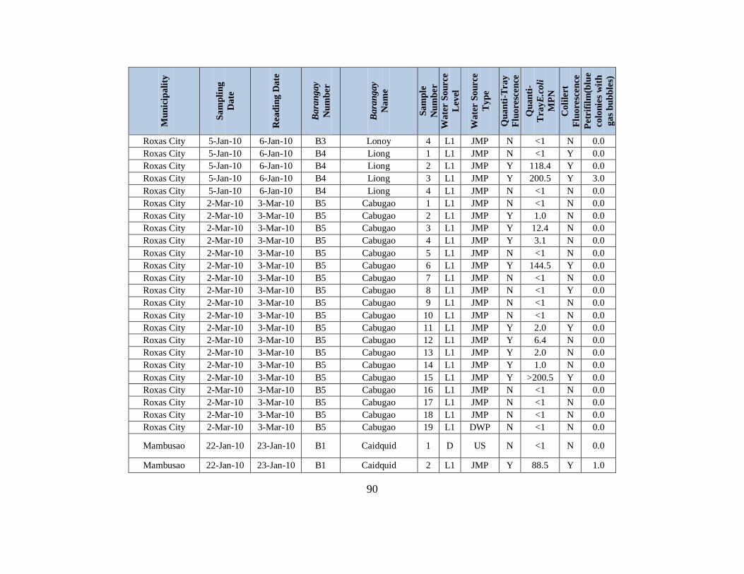
90
Mu
nic
ipali
ty
Sa
mp
lin
g
Da
te
Rea
din
g D
ate
Ba
ran
gay
Nu
mb
er
Ba
ran
gay
Na
me
Sa
mp
le
Nu
mb
er
Wa
ter S
ou
rce
Lev
el
Wa
ter S
ou
rce
Ty
pe
Qu
an
ti-T
ray
Flu
ore
scen
ce
Qu
an
ti-
Tra
yE
.coli
MP
N
Co
lile
rt
Flu
ore
scen
ce
Petr
ifil
m(b
lue
co
lon
ies
wit
h
ga
s b
ub
ble
s)
Roxas City 5-Jan-10 6-Jan-10 B3 Lonoy 4 L1 JMP N <1 N 0.0
Roxas City 5-Jan-10 6-Jan-10 B4 Liong 1 L1 JMP N <1 Y 0.0
Roxas City 5-Jan-10 6-Jan-10 B4 Liong 2 L1 JMP Y 118.4 Y 0.0
Roxas City 5-Jan-10 6-Jan-10 B4 Liong 3 L1 JMP Y 200.5 Y 3.0
Roxas City 5-Jan-10 6-Jan-10 B4 Liong 4 L1 JMP N <1 N 0.0
Roxas City 2-Mar-10 3-Mar-10 B5 Cabugao 1 L1 JMP N <1 N 0.0
Roxas City 2-Mar-10 3-Mar-10 B5 Cabugao 2 L1 JMP Y 1.0 N 0.0
Roxas City 2-Mar-10 3-Mar-10 B5 Cabugao 3 L1 JMP Y 12.4 N 0.0
Roxas City 2-Mar-10 3-Mar-10 B5 Cabugao 4 L1 JMP Y 3.1 N 0.0
Roxas City 2-Mar-10 3-Mar-10 B5 Cabugao 5 L1 JMP N <1 N 0.0
Roxas City 2-Mar-10 3-Mar-10 B5 Cabugao 6 L1 JMP Y 144.5 Y 0.0
Roxas City 2-Mar-10 3-Mar-10 B5 Cabugao 7 L1 JMP N <1 N 0.0
Roxas City 2-Mar-10 3-Mar-10 B5 Cabugao 8 L1 JMP N <1 Y 0.0
Roxas City 2-Mar-10 3-Mar-10 B5 Cabugao 9 L1 JMP N <1 N 0.0
Roxas City 2-Mar-10 3-Mar-10 B5 Cabugao 10 L1 JMP N <1 N 0.0
Roxas City 2-Mar-10 3-Mar-10 B5 Cabugao 11 L1 JMP Y 2.0 Y 0.0
Roxas City 2-Mar-10 3-Mar-10 B5 Cabugao 12 L1 JMP Y 6.4 N 0.0
Roxas City 2-Mar-10 3-Mar-10 B5 Cabugao 13 L1 JMP Y 2.0 N 0.0
Roxas City 2-Mar-10 3-Mar-10 B5 Cabugao 14 L1 JMP Y 1.0 N 0.0
Roxas City 2-Mar-10 3-Mar-10 B5 Cabugao 15 L1 JMP Y >200.5 Y 0.0
Roxas City 2-Mar-10 3-Mar-10 B5 Cabugao 16 L1 JMP N <1 N 0.0
Roxas City 2-Mar-10 3-Mar-10 B5 Cabugao 17 L1 JMP N <1 N 0.0
Roxas City 2-Mar-10 3-Mar-10 B5 Cabugao 18 L1 JMP N <1 N 0.0
Roxas City 2-Mar-10 3-Mar-10 B5 Cabugao 19 L1 DWP N <1 N 0.0
Mambusao 22-Jan-10 23-Jan-10 B1 Caidquid 1 D US N <1 N 0.0
Mambusao 22-Jan-10 23-Jan-10 B1 Caidquid 2 L1 JMP Y 88.5 Y 1.0
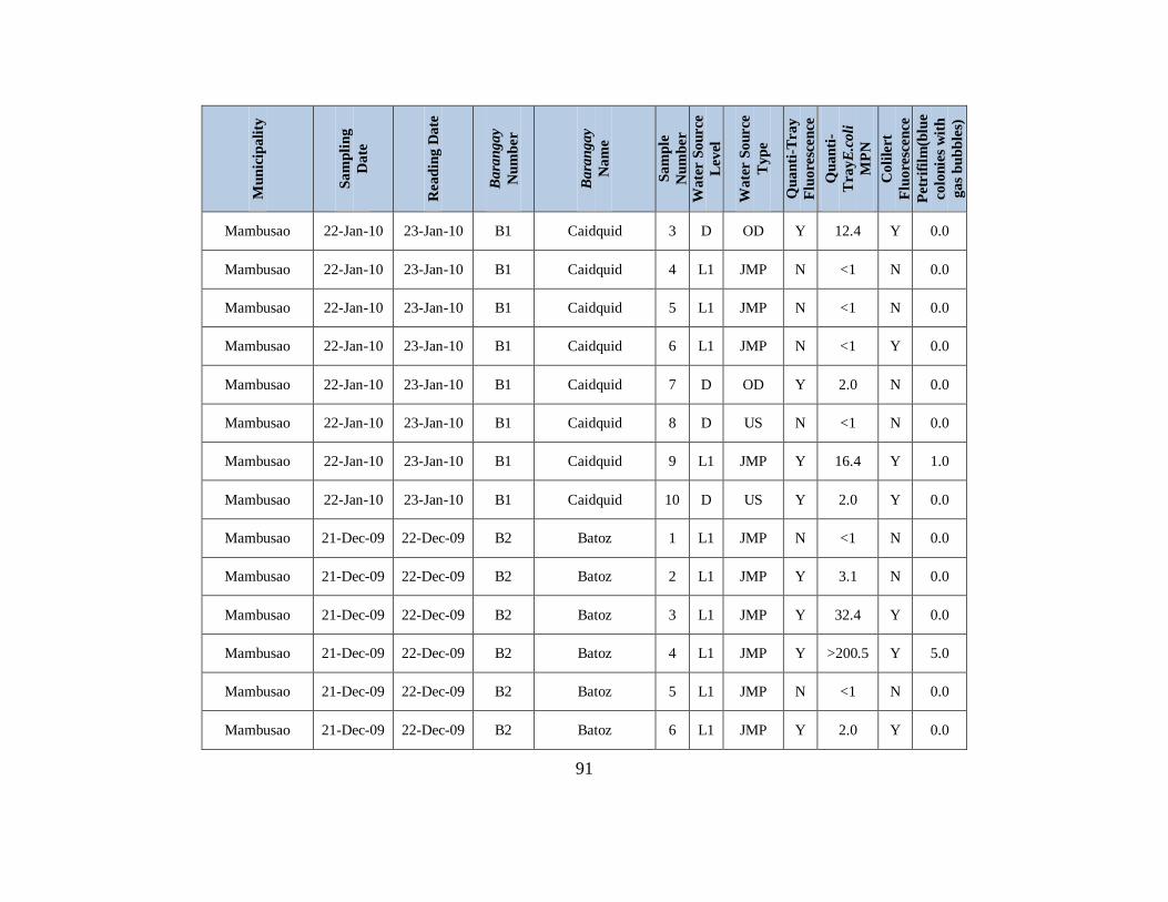
91
Mu
nic
ipali
ty
Sa
mp
lin
g
Da
te
Rea
din
g D
ate
Ba
ran
gay
Nu
mb
er
Ba
ran
gay
Na
me
Sa
mp
le
Nu
mb
er
Wa
ter S
ou
rce
Lev
el
Wa
ter S
ou
rce
Ty
pe
Qu
an
ti-T
ray
Flu
ore
scen
ce
Qu
an
ti-
Tra
yE
.coli
MP
N
Co
lile
rt
Flu
ore
scen
ce
Petr
ifil
m(b
lue
co
lon
ies
wit
h
ga
s b
ub
ble
s)
Mambusao 22-Jan-10 23-Jan-10 B1 Caidquid 3 D OD Y 12.4 Y 0.0
Mambusao 22-Jan-10 23-Jan-10 B1 Caidquid 4 L1 JMP N <1 N 0.0
Mambusao 22-Jan-10 23-Jan-10 B1 Caidquid 5 L1 JMP N <1 N 0.0
Mambusao 22-Jan-10 23-Jan-10 B1 Caidquid 6 L1 JMP N <1 Y 0.0
Mambusao 22-Jan-10 23-Jan-10 B1 Caidquid 7 D OD Y 2.0 N 0.0
Mambusao 22-Jan-10 23-Jan-10 B1 Caidquid 8 D US N <1 N 0.0
Mambusao 22-Jan-10 23-Jan-10 B1 Caidquid 9 L1 JMP Y 16.4 Y 1.0
Mambusao 22-Jan-10 23-Jan-10 B1 Caidquid 10 D US Y 2.0 Y 0.0
Mambusao 21-Dec-09 22-Dec-09 B2 Batoz 1 L1 JMP N <1 N 0.0
Mambusao 21-Dec-09 22-Dec-09 B2 Batoz 2 L1 JMP Y 3.1 N 0.0
Mambusao 21-Dec-09 22-Dec-09 B2 Batoz 3 L1 JMP Y 32.4 Y 0.0
Mambusao 21-Dec-09 22-Dec-09 B2 Batoz 4 L1 JMP Y >200.5 Y 5.0
Mambusao 21-Dec-09 22-Dec-09 B2 Batoz 5 L1 JMP N <1 N 0.0
Mambusao 21-Dec-09 22-Dec-09 B2 Batoz 6 L1 JMP Y 2.0 Y 0.0
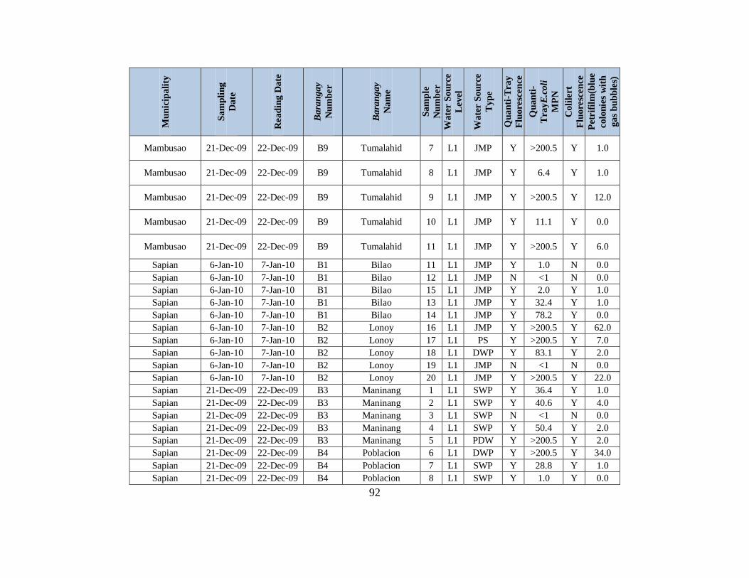
92
Mu
nic
ipali
ty
Sa
mp
lin
g
Da
te
Rea
din
g D
ate
Ba
ran
gay
Nu
mb
er
Ba
ran
gay
Na
me
Sa
mp
le
Nu
mb
er
Wa
ter S
ou
rce
Lev
el
Wa
ter S
ou
rce
Ty
pe
Qu
an
ti-T
ray
Flu
ore
scen
ce
Qu
an
ti-
Tra
yE
.coli
MP
N
Co
lile
rt
Flu
ore
scen
ce
Petr
ifil
m(b
lue
co
lon
ies
wit
h
ga
s b
ub
ble
s)
Mambusao 21-Dec-09 22-Dec-09 B9 Tumalahid 7 L1 JMP Y >200.5 Y 1.0
Mambusao 21-Dec-09 22-Dec-09 B9 Tumalahid 8 L1 JMP Y 6.4 Y 1.0
Mambusao 21-Dec-09 22-Dec-09 B9 Tumalahid 9 L1 JMP Y >200.5 Y 12.0
Mambusao 21-Dec-09 22-Dec-09 B9 Tumalahid 10 L1 JMP Y 11.1 Y 0.0
Mambusao 21-Dec-09 22-Dec-09 B9 Tumalahid 11 L1 JMP Y >200.5 Y 6.0
Sapian 6-Jan-10 7-Jan-10 B1 Bilao 11 L1 JMP Y 1.0 N 0.0
Sapian 6-Jan-10 7-Jan-10 B1 Bilao 12 L1 JMP N <1 N 0.0
Sapian 6-Jan-10 7-Jan-10 B1 Bilao 15 L1 JMP Y 2.0 Y 1.0
Sapian 6-Jan-10 7-Jan-10 B1 Bilao 13 L1 JMP Y 32.4 Y 1.0
Sapian 6-Jan-10 7-Jan-10 B1 Bilao 14 L1 JMP Y 78.2 Y 0.0
Sapian 6-Jan-10 7-Jan-10 B2 Lonoy 16 L1 JMP Y >200.5 Y 62.0
Sapian 6-Jan-10 7-Jan-10 B2 Lonoy 17 L1 PS Y >200.5 Y 7.0
Sapian 6-Jan-10 7-Jan-10 B2 Lonoy 18 L1 DWP Y 83.1 Y 2.0
Sapian 6-Jan-10 7-Jan-10 B2 Lonoy 19 L1 JMP N <1 N 0.0
Sapian 6-Jan-10 7-Jan-10 B2 Lonoy 20 L1 JMP Y >200.5 Y 22.0
Sapian 21-Dec-09 22-Dec-09 B3 Maninang 1 L1 SWP Y 36.4 Y 1.0
Sapian 21-Dec-09 22-Dec-09 B3 Maninang 2 L1 SWP Y 40.6 Y 4.0
Sapian 21-Dec-09 22-Dec-09 B3 Maninang 3 L1 SWP N <1 N 0.0
Sapian 21-Dec-09 22-Dec-09 B3 Maninang 4 L1 SWP Y 50.4 Y 2.0
Sapian 21-Dec-09 22-Dec-09 B3 Maninang 5 L1 PDW Y >200.5 Y 2.0
Sapian 21-Dec-09 22-Dec-09 B4 Poblacion 6 L1 DWP Y >200.5 Y 34.0
Sapian 21-Dec-09 22-Dec-09 B4 Poblacion 7 L1 SWP Y 28.8 Y 1.0
Sapian 21-Dec-09 22-Dec-09 B4 Poblacion 8 L1 SWP Y 1.0 Y 0.0
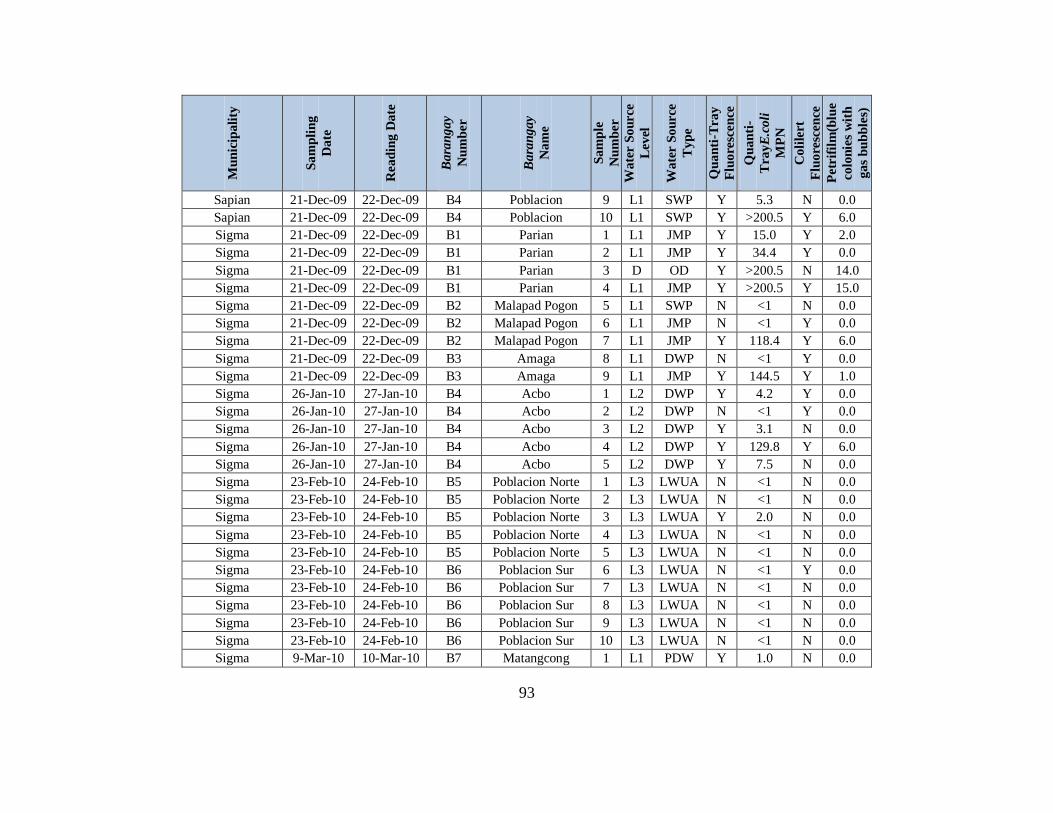
93
Mu
nic
ipali
ty
Sa
mp
lin
g
Da
te
Rea
din
g D
ate
Ba
ran
gay
Nu
mb
er
Ba
ran
gay
Na
me
Sa
mp
le
Nu
mb
er
Wa
ter S
ou
rce
Lev
el
Wa
ter S
ou
rce
Ty
pe
Qu
an
ti-T
ray
Flu
ore
scen
ce
Qu
an
ti-
Tra
yE
.coli
MP
N
Co
lile
rt
Flu
ore
scen
ce
Petr
ifil
m(b
lue
co
lon
ies
wit
h
ga
s b
ub
ble
s)
Sapian 21-Dec-09 22-Dec-09 B4 Poblacion 9 L1 SWP Y 5.3 N 0.0
Sapian 21-Dec-09 22-Dec-09 B4 Poblacion 10 L1 SWP Y >200.5 Y 6.0
Sigma 21-Dec-09 22-Dec-09 B1 Parian 1 L1 JMP Y 15.0 Y 2.0
Sigma 21-Dec-09 22-Dec-09 B1 Parian 2 L1 JMP Y 34.4 Y 0.0
Sigma 21-Dec-09 22-Dec-09 B1 Parian 3 D OD Y >200.5 N 14.0
Sigma 21-Dec-09 22-Dec-09 B1 Parian 4 L1 JMP Y >200.5 Y 15.0
Sigma 21-Dec-09 22-Dec-09 B2 Malapad Pogon 5 L1 SWP N <1 N 0.0
Sigma 21-Dec-09 22-Dec-09 B2 Malapad Pogon 6 L1 JMP N <1 Y 0.0
Sigma 21-Dec-09 22-Dec-09 B2 Malapad Pogon 7 L1 JMP Y 118.4 Y 6.0
Sigma 21-Dec-09 22-Dec-09 B3 Amaga 8 L1 DWP N <1 Y 0.0
Sigma 21-Dec-09 22-Dec-09 B3 Amaga 9 L1 JMP Y 144.5 Y 1.0
Sigma 26-Jan-10 27-Jan-10 B4 Acbo 1 L2 DWP Y 4.2 Y 0.0
Sigma 26-Jan-10 27-Jan-10 B4 Acbo 2 L2 DWP N <1 Y 0.0
Sigma 26-Jan-10 27-Jan-10 B4 Acbo 3 L2 DWP Y 3.1 N 0.0
Sigma 26-Jan-10 27-Jan-10 B4 Acbo 4 L2 DWP Y 129.8 Y 6.0
Sigma 26-Jan-10 27-Jan-10 B4 Acbo 5 L2 DWP Y 7.5 N 0.0
Sigma 23-Feb-10 24-Feb-10 B5 Poblacion Norte 1 L3 LWUA N <1 N 0.0
Sigma 23-Feb-10 24-Feb-10 B5 Poblacion Norte 2 L3 LWUA N <1 N 0.0
Sigma 23-Feb-10 24-Feb-10 B5 Poblacion Norte 3 L3 LWUA Y 2.0 N 0.0
Sigma 23-Feb-10 24-Feb-10 B5 Poblacion Norte 4 L3 LWUA N <1 N 0.0
Sigma 23-Feb-10 24-Feb-10 B5 Poblacion Norte 5 L3 LWUA N <1 N 0.0
Sigma 23-Feb-10 24-Feb-10 B6 Poblacion Sur 6 L3 LWUA N <1 Y 0.0
Sigma 23-Feb-10 24-Feb-10 B6 Poblacion Sur 7 L3 LWUA N <1 N 0.0
Sigma 23-Feb-10 24-Feb-10 B6 Poblacion Sur 8 L3 LWUA N <1 N 0.0
Sigma 23-Feb-10 24-Feb-10 B6 Poblacion Sur 9 L3 LWUA N <1 N 0.0
Sigma 23-Feb-10 24-Feb-10 B6 Poblacion Sur 10 L3 LWUA N <1 N 0.0
Sigma 9-Mar-10 10-Mar-10 B7 Matangcong 1 L1 PDW Y 1.0 N 0.0
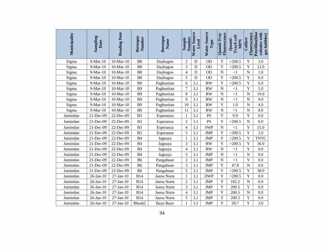
94
Mu
nic
ipali
ty
Sa
mp
lin
g
Da
te
Rea
din
g D
ate
Ba
ran
gay
Nu
mb
er
Ba
ran
gay
Na
me
Sa
mp
le
Nu
mb
er
Wa
ter S
ou
rce
Lev
el
Wa
ter S
ou
rce
Ty
pe
Qu
an
ti-T
ray
Flu
ore
scen
ce
Qu
an
ti-
Tra
yE
.coli
MP
N
Co
lile
rt
Flu
ore
scen
ce
Petr
ifil
m(b
lue
co
lon
ies
wit
h
ga
s b
ub
ble
s)
Sigma 9-Mar-10 10-Mar-10 B8 Dayhagon 2 D OD Y >200.5 Y 3.0
Sigma 9-Mar-10 10-Mar-10 B8 Dayhagon 3 D OD Y >200.5 Y 12.0
Sigma 9-Mar-10 10-Mar-10 B8 Dayhagon 4 D OD N <1 N 1.0
Sigma 9-Mar-10 10-Mar-10 B8 Dayhagon 5 D OD Y >200.5 Y 0.0
Sigma 9-Mar-10 10-Mar-10 B9 Pagbunitan 6 L1 RW Y >200.5 Y 6.0
Sigma 9-Mar-10 10-Mar-10 B9 Pagbunitan 7 L1 RW N <1 Y 5.0
Sigma 9-Mar-10 10-Mar-10 B9 Pagbunitan 8 L1 RW N <1 N 10.0
Sigma 9-Mar-10 10-Mar-10 B9 Pagbunitan 9 L1 RW N <1 N 9.0
Sigma 9-Mar-10 10-Mar-10 B9 Pagbunitan 10 L1 RW Y 1.0 N 4.0
Sigma 9-Mar-10 10-Mar-10 B9 Pagbunitan 11 L1 RW N <1 N 8.0
Jamindan 21-Dec-09 22-Dec-09 B3 Esperanza 1 L1 PS Y 9.9 Y 0.0
Jamindan 21-Dec-09 22-Dec-09 B3 Esperanza 2 L1 PS Y >200.5 N 0.0
Jamindan 21-Dec-09 22-Dec-09 B3 Esperanza 4 L1 SWP N <1 Y 15.0
Jamindan 21-Dec-09 22-Dec-09 B3 Esperanza 5 L1 JMP Y >200.5 Y 2.0
Jamindan 21-Dec-09 22-Dec-09 B4 Jagnaya 1 L1 JMP Y >200.5 Y TNTC
Jamindan 21-Dec-09 22-Dec-09 B4 Jagnaya 3 L1 RW Y >200.5 Y 36.0
Jamindan 21-Dec-09 22-Dec-09 B4 Jagnaya 4 L1 RW N <1 Y 0.0
Jamindan 21-Dec-09 22-Dec-09 B4 Jagnaya 5 L1 JMP N <1 N 0.0
Jamindan 21-Dec-09 22-Dec-09 B6 Pangabuan 2 L1 JMP N <1 Y 0.0
Jamindan 21-Dec-09 22-Dec-09 B6 Pangabuan 3 L1 JMP Y 47.8 N 0.0
Jamindan 21-Dec-09 22-Dec-09 B6 Pangabuan 5 L1 JMP Y >200.5 Y 38.0
Jamindan 26-Jan-10 27-Jan-10 B14 Jaena Norte 1 L1 DWP Y >200.5 Y 0.0
Jamindan 26-Jan-10 27-Jan-10 B14 Jaena Norte 2 L1 JMP Y 165.2 N 0.0
Jamindan 26-Jan-10 27-Jan-10 B14 Jaena Norte 3 L1 JMP Y 200.5 Y 0.0
Jamindan 26-Jan-10 27-Jan-10 B14 Jaena Norte 4 L1 JMP Y 200.5 N 0.0
Jamindan 26-Jan-10 27-Jan-10 B14 Jaena Norte 5 L1 JMP Y 200.5 Y 0.0
Jamindan 26-Jan-10 27-Jan-10 B6sub2 Baye Baye 1 L1 JMP Y 59.7 Y 3.0
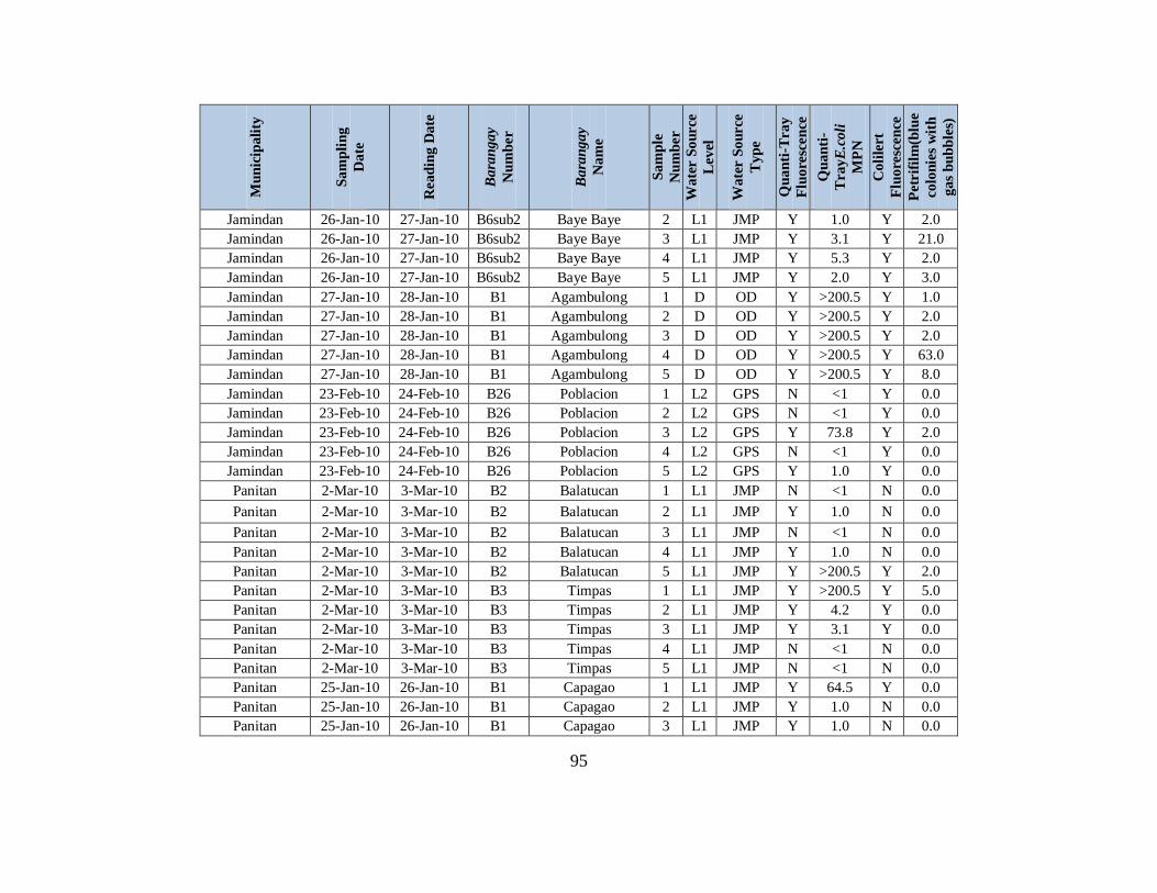
95
Mu
nic
ipali
ty
Sa
mp
lin
g
Da
te
Rea
din
g D
ate
Ba
ran
gay
Nu
mb
er
Ba
ran
gay
Na
me
Sa
mp
le
Nu
mb
er
Wa
ter S
ou
rce
Lev
el
Wa
ter S
ou
rce
Ty
pe
Qu
an
ti-T
ray
Flu
ore
scen
ce
Qu
an
ti-
Tra
yE
.coli
MP
N
Co
lile
rt
Flu
ore
scen
ce
Petr
ifil
m(b
lue
co
lon
ies
wit
h
ga
s b
ub
ble
s)
Jamindan 26-Jan-10 27-Jan-10 B6sub2 Baye Baye 2 L1 JMP Y 1.0 Y 2.0
Jamindan 26-Jan-10 27-Jan-10 B6sub2 Baye Baye 3 L1 JMP Y 3.1 Y 21.0
Jamindan 26-Jan-10 27-Jan-10 B6sub2 Baye Baye 4 L1 JMP Y 5.3 Y 2.0
Jamindan 26-Jan-10 27-Jan-10 B6sub2 Baye Baye 5 L1 JMP Y 2.0 Y 3.0
Jamindan 27-Jan-10 28-Jan-10 B1 Agambulong 1 D OD Y >200.5 Y 1.0
Jamindan 27-Jan-10 28-Jan-10 B1 Agambulong 2 D OD Y >200.5 Y 2.0
Jamindan 27-Jan-10 28-Jan-10 B1 Agambulong 3 D OD Y >200.5 Y 2.0
Jamindan 27-Jan-10 28-Jan-10 B1 Agambulong 4 D OD Y >200.5 Y 63.0
Jamindan 27-Jan-10 28-Jan-10 B1 Agambulong 5 D OD Y >200.5 Y 8.0
Jamindan 23-Feb-10 24-Feb-10 B26 Poblacion 1 L2 GPS N <1 Y 0.0
Jamindan 23-Feb-10 24-Feb-10 B26 Poblacion 2 L2 GPS N <1 Y 0.0
Jamindan 23-Feb-10 24-Feb-10 B26 Poblacion 3 L2 GPS Y 73.8 Y 2.0
Jamindan 23-Feb-10 24-Feb-10 B26 Poblacion 4 L2 GPS N <1 Y 0.0
Jamindan 23-Feb-10 24-Feb-10 B26 Poblacion 5 L2 GPS Y 1.0 Y 0.0
Panitan 2-Mar-10 3-Mar-10 B2 Balatucan 1 L1 JMP N <1 N 0.0
Panitan 2-Mar-10 3-Mar-10 B2 Balatucan 2 L1 JMP Y 1.0 N 0.0
Panitan 2-Mar-10 3-Mar-10 B2 Balatucan 3 L1 JMP N <1 N 0.0
Panitan 2-Mar-10 3-Mar-10 B2 Balatucan 4 L1 JMP Y 1.0 N 0.0
Panitan 2-Mar-10 3-Mar-10 B2 Balatucan 5 L1 JMP Y >200.5 Y 2.0
Panitan 2-Mar-10 3-Mar-10 B3 Timpas 1 L1 JMP Y >200.5 Y 5.0
Panitan 2-Mar-10 3-Mar-10 B3 Timpas 2 L1 JMP Y 4.2 Y 0.0
Panitan 2-Mar-10 3-Mar-10 B3 Timpas 3 L1 JMP Y 3.1 Y 0.0
Panitan 2-Mar-10 3-Mar-10 B3 Timpas 4 L1 JMP N <1 N 0.0
Panitan 2-Mar-10 3-Mar-10 B3 Timpas 5 L1 JMP N <1 N 0.0
Panitan 25-Jan-10 26-Jan-10 B1 Capagao 1 L1 JMP Y 64.5 Y 0.0
Panitan 25-Jan-10 26-Jan-10 B1 Capagao 2 L1 JMP Y 1.0 N 0.0
Panitan 25-Jan-10 26-Jan-10 B1 Capagao 3 L1 JMP Y 1.0 N 0.0
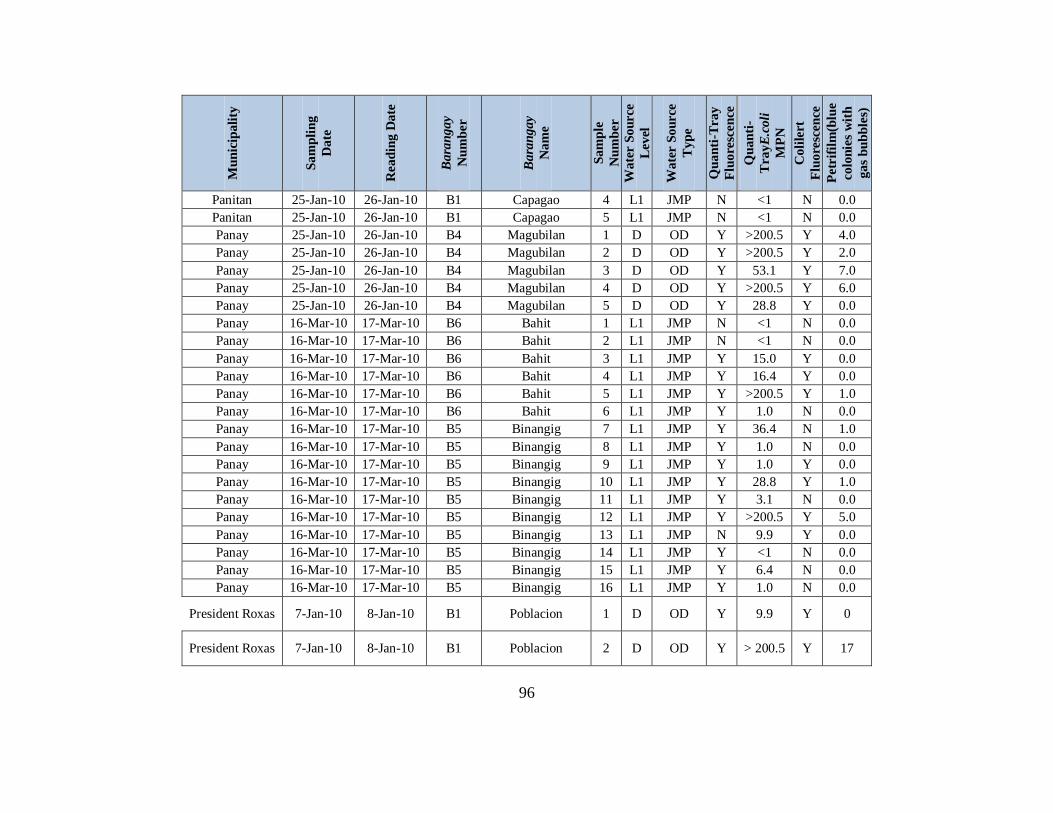
96
Mu
nic
ipali
ty
Sa
mp
lin
g
Da
te
Rea
din
g D
ate
Ba
ran
gay
Nu
mb
er
Ba
ran
gay
Na
me
Sa
mp
le
Nu
mb
er
Wa
ter S
ou
rce
Lev
el
Wa
ter S
ou
rce
Ty
pe
Qu
an
ti-T
ray
Flu
ore
scen
ce
Qu
an
ti-
Tra
yE
.coli
MP
N
Co
lile
rt
Flu
ore
scen
ce
Petr
ifil
m(b
lue
co
lon
ies
wit
h
ga
s b
ub
ble
s)
Panitan 25-Jan-10 26-Jan-10 B1 Capagao 4 L1 JMP N <1 N 0.0
Panitan 25-Jan-10 26-Jan-10 B1 Capagao 5 L1 JMP N <1 N 0.0
Panay 25-Jan-10 26-Jan-10 B4 Magubilan 1 D OD Y >200.5 Y 4.0
Panay 25-Jan-10 26-Jan-10 B4 Magubilan 2 D OD Y >200.5 Y 2.0
Panay 25-Jan-10 26-Jan-10 B4 Magubilan 3 D OD Y 53.1 Y 7.0
Panay 25-Jan-10 26-Jan-10 B4 Magubilan 4 D OD Y >200.5 Y 6.0
Panay 25-Jan-10 26-Jan-10 B4 Magubilan 5 D OD Y 28.8 Y 0.0
Panay 16-Mar-10 17-Mar-10 B6 Bahit 1 L1 JMP N <1 N 0.0
Panay 16-Mar-10 17-Mar-10 B6 Bahit 2 L1 JMP N <1 N 0.0
Panay 16-Mar-10 17-Mar-10 B6 Bahit 3 L1 JMP Y 15.0 Y 0.0
Panay 16-Mar-10 17-Mar-10 B6 Bahit 4 L1 JMP Y 16.4 Y 0.0
Panay 16-Mar-10 17-Mar-10 B6 Bahit 5 L1 JMP Y >200.5 Y 1.0
Panay 16-Mar-10 17-Mar-10 B6 Bahit 6 L1 JMP Y 1.0 N 0.0
Panay 16-Mar-10 17-Mar-10 B5 Binangig 7 L1 JMP Y 36.4 N 1.0
Panay 16-Mar-10 17-Mar-10 B5 Binangig 8 L1 JMP Y 1.0 N 0.0
Panay 16-Mar-10 17-Mar-10 B5 Binangig 9 L1 JMP Y 1.0 Y 0.0
Panay 16-Mar-10 17-Mar-10 B5 Binangig 10 L1 JMP Y 28.8 Y 1.0
Panay 16-Mar-10 17-Mar-10 B5 Binangig 11 L1 JMP Y 3.1 N 0.0
Panay 16-Mar-10 17-Mar-10 B5 Binangig 12 L1 JMP Y >200.5 Y 5.0
Panay 16-Mar-10 17-Mar-10 B5 Binangig 13 L1 JMP N 9.9 Y 0.0
Panay 16-Mar-10 17-Mar-10 B5 Binangig 14 L1 JMP Y <1 N 0.0
Panay 16-Mar-10 17-Mar-10 B5 Binangig 15 L1 JMP Y 6.4 N 0.0
Panay 16-Mar-10 17-Mar-10 B5 Binangig 16 L1 JMP Y 1.0 N 0.0
President Roxas 7-Jan-10 8-Jan-10 B1 Poblacion 1 D OD Y 9.9 Y 0
President Roxas 7-Jan-10 8-Jan-10 B1 Poblacion 2 D OD Y > 200.5 Y 17
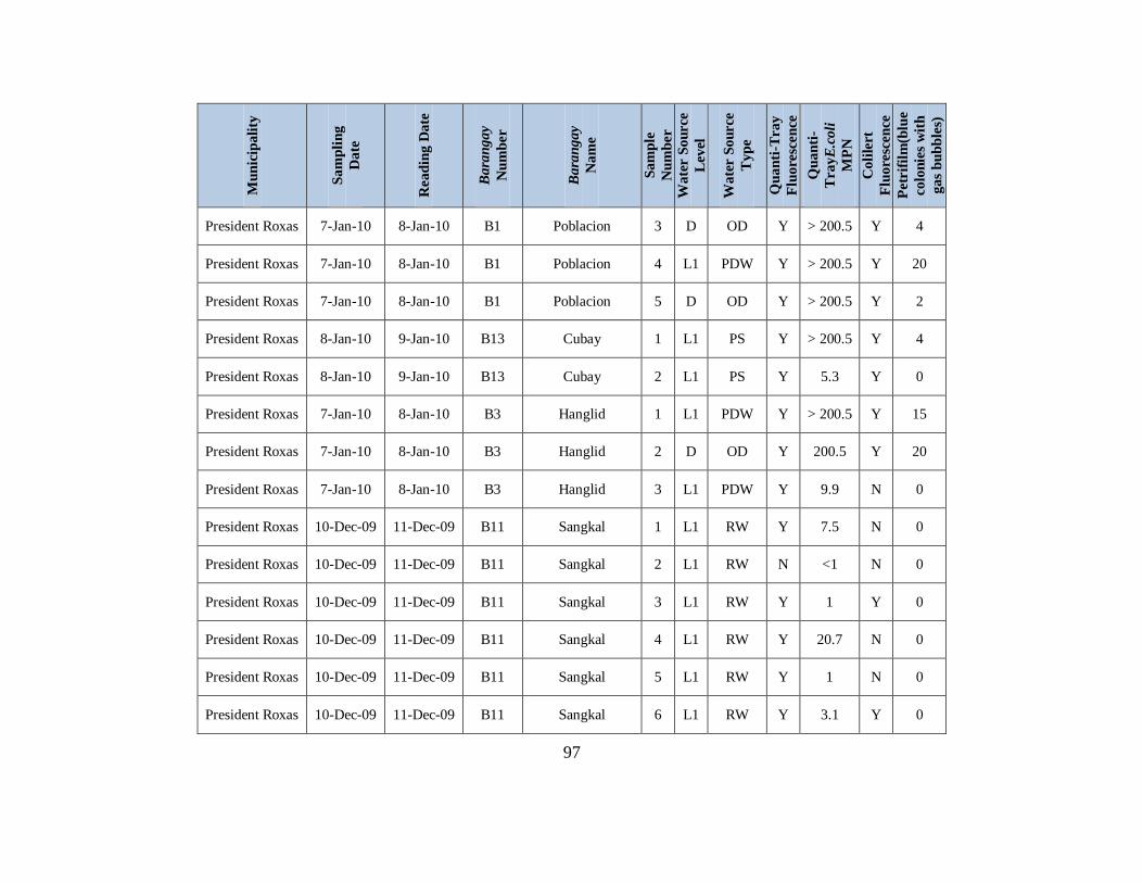
97
Mu
nic
ipali
ty
Sa
mp
lin
g
Da
te
Rea
din
g D
ate
Ba
ran
gay
Nu
mb
er
Ba
ran
gay
Na
me
Sa
mp
le
Nu
mb
er
Wa
ter S
ou
rce
Lev
el
Wa
ter S
ou
rce
Ty
pe
Qu
an
ti-T
ray
Flu
ore
scen
ce
Qu
an
ti-
Tra
yE
.coli
MP
N
Co
lile
rt
Flu
ore
scen
ce
Petr
ifil
m(b
lue
co
lon
ies
wit
h
ga
s b
ub
ble
s)
President Roxas 7-Jan-10 8-Jan-10 B1 Poblacion 3 D OD Y > 200.5 Y 4
President Roxas 7-Jan-10 8-Jan-10 B1 Poblacion 4 L1 PDW Y > 200.5 Y 20
President Roxas 7-Jan-10 8-Jan-10 B1 Poblacion 5 D OD Y > 200.5 Y 2
President Roxas 8-Jan-10 9-Jan-10 B13 Cubay 1 L1 PS Y > 200.5 Y 4
President Roxas 8-Jan-10 9-Jan-10 B13 Cubay 2 L1 PS Y 5.3 Y 0
President Roxas 7-Jan-10 8-Jan-10 B3 Hanglid 1 L1 PDW Y > 200.5 Y 15
President Roxas 7-Jan-10 8-Jan-10 B3 Hanglid 2 D OD Y 200.5 Y 20
President Roxas 7-Jan-10 8-Jan-10 B3 Hanglid 3 L1 PDW Y 9.9 N 0
President Roxas 10-Dec-09 11-Dec-09 B11 Sangkal 1 L1 RW Y 7.5 N 0
President Roxas 10-Dec-09 11-Dec-09 B11 Sangkal 2 L1 RW N <1 N 0
President Roxas 10-Dec-09 11-Dec-09 B11 Sangkal 3 L1 RW Y 1 Y 0
President Roxas 10-Dec-09 11-Dec-09 B11 Sangkal 4 L1 RW Y 20.7 N 0
President Roxas 10-Dec-09 11-Dec-09 B11 Sangkal 5 L1 RW Y 1 N 0
President Roxas 10-Dec-09 11-Dec-09 B11 Sangkal 6 L1 RW Y 3.1 Y 0
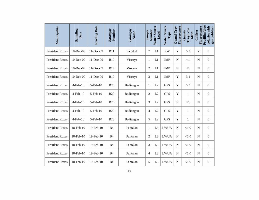
98
Mu
nic
ipali
ty
Sa
mp
lin
g
Da
te
Rea
din
g D
ate
Ba
ran
gay
Nu
mb
er
Ba
ran
gay
Na
me
Sa
mp
le
Nu
mb
er
Wa
ter S
ou
rce
Lev
el
Wa
ter S
ou
rce
Ty
pe
Qu
an
ti-T
ray
Flu
ore
scen
ce
Qu
an
ti-
Tra
yE
.coli
MP
N
Co
lile
rt
Flu
ore
scen
ce
Petr
ifil
m(b
lue
co
lon
ies
wit
h
ga
s b
ub
ble
s)
President Roxas 10-Dec-09 11-Dec-09 B11 Sangkal 7 L1 RW Y 5.3 Y 0
President Roxas 10-Dec-09 11-Dec-09 B19 Viscaya 1 L1 JMP N <1 N 0
President Roxas 10-Dec-09 11-Dec-09 B19 Viscaya 2 L1 JMP N <1 N 0
President Roxas 10-Dec-09 11-Dec-09 B19 Viscaya 3 L1 JMP Y 3.1 N 0
President Roxas 4-Feb-10 5-Feb-10 B20 Badiangon 1 L2 GPS Y 5.3 N 0
President Roxas 4-Feb-10 5-Feb-10 B20 Badiangon 2 L2 GPS Y 1 N 0
President Roxas 4-Feb-10 5-Feb-10 B20 Badiangon 3 L2 GPS N <1 N 0
President Roxas 4-Feb-10 5-Feb-10 B20 Badiangon 4 L2 GPS Y 1 N 0
President Roxas 4-Feb-10 5-Feb-10 B20 Badiangon 5 L2 GPS Y 1 N 0
President Roxas 18-Feb-10 19-Feb-10 B4 Pantalan 1 L3 LWUA N <1.0 N 0
President Roxas 18-Feb-10 19-Feb-10 B4 Pantalan 2 L3 LWUA N <1.0 N 0
President Roxas 18-Feb-10 19-Feb-10 B4 Pantalan 3 L3 LWUA N <1.0 N 0
President Roxas 18-Feb-10 19-Feb-10 B4 Pantalan 4 L3 LWUA N <1.0 N 0
President Roxas 18-Feb-10 19-Feb-10 B4 Pantalan 5 L3 LWUA N <1.0 N 0
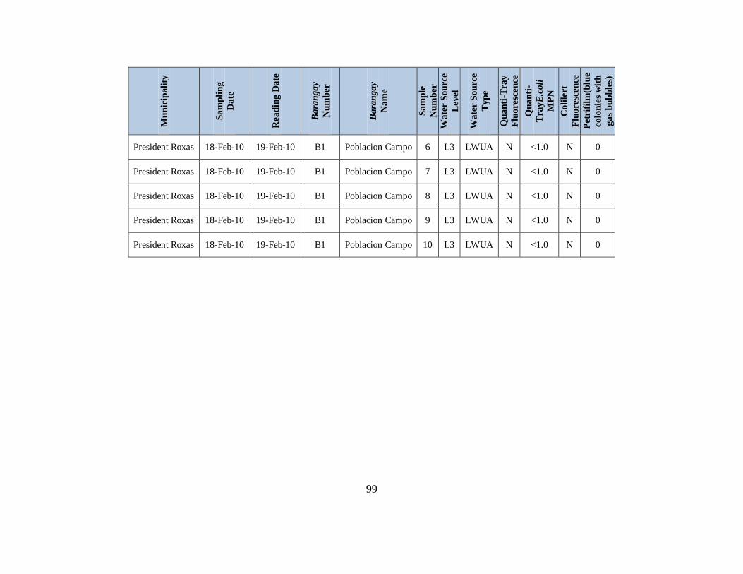
99
Mu
nic
ipali
ty
Sa
mp
lin
g
Da
te
Rea
din
g D
ate
Ba
ran
gay
Nu
mb
er
Ba
ran
gay
Na
me
Sa
mp
le
Nu
mb
er
Wa
ter S
ou
rce
Lev
el
Wa
ter S
ou
rce
Ty
pe
Qu
an
ti-T
ray
Flu
ore
scen
ce
Qu
an
ti-
Tra
yE
.coli
MP
N
Co
lile
rt
Flu
ore
scen
ce
Petr
ifil
m(b
lue
co
lon
ies
wit
h
ga
s b
ub
ble
s)
President Roxas 18-Feb-10 19-Feb-10 B1 Poblacion Campo 6 L3 LWUA N <1.0 N 0
President Roxas 18-Feb-10 19-Feb-10 B1 Poblacion Campo 7 L3 LWUA N <1.0 N 0
President Roxas 18-Feb-10 19-Feb-10 B1 Poblacion Campo 8 L3 LWUA N <1.0 N 0
President Roxas 18-Feb-10 19-Feb-10 B1 Poblacion Campo 9 L3 LWUA N <1.0 N 0
President Roxas 18-Feb-10 19-Feb-10 B1 Poblacion Campo 10 L3 LWUA N <1.0 N 0

100
Appendix C: Charles River Water Quality Results
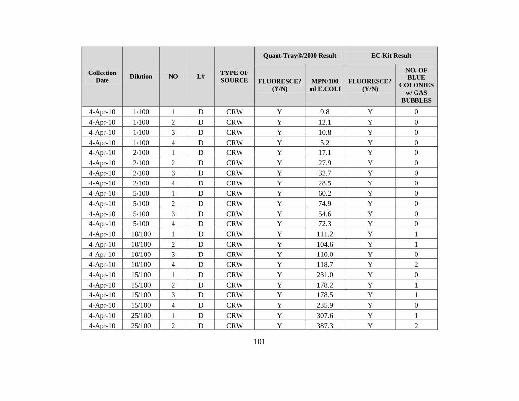
101
Collection
Date Dilution NO L#
TYPE OF
SOURCE
Quant-Tray®/2000 Result EC-Kit Result
FLUORESCE?
(Y/N)
MPN/100
ml E.COLI
FLUORESCE?
(Y/N)
NO. OF
BLUE
COLONIES
w/ GAS
BUBBLES
4-Apr-10 1/100 1 D CRW Y 9.8 Y 0
4-Apr-10 1/100 2 D CRW Y 12.1 Y 0
4-Apr-10 1/100 3 D CRW Y 10.8 Y 0
4-Apr-10 1/100 4 D CRW Y 5.2 Y 0
4-Apr-10 2/100 1 D CRW Y 17.1 Y 0
4-Apr-10 2/100 2 D CRW Y 27.9 Y 0
4-Apr-10 2/100 3 D CRW Y 32.7 Y 0
4-Apr-10 2/100 4 D CRW Y 28.5 Y 0
4-Apr-10 5/100 1 D CRW Y 60.2 Y 0
4-Apr-10 5/100 2 D CRW Y 74.9 Y 0
4-Apr-10 5/100 3 D CRW Y 54.6 Y 0
4-Apr-10 5/100 4 D CRW Y 72.3 Y 0
4-Apr-10 10/100 1 D CRW Y 111.2 Y 1
4-Apr-10 10/100 2 D CRW Y 104.6 Y 1
4-Apr-10 10/100 3 D CRW Y 110.0 Y 0
4-Apr-10 10/100 4 D CRW Y 118.7 Y 2
4-Apr-10 15/100 1 D CRW Y 231.0 Y 0
4-Apr-10 15/100 2 D CRW Y 178.2 Y 1
4-Apr-10 15/100 3 D CRW Y 178.5 Y 1
4-Apr-10 15/100 4 D CRW Y 235.9 Y 0
4-Apr-10 25/100 1 D CRW Y 307.6 Y 1
4-Apr-10 25/100 2 D CRW Y 387.3 Y 2
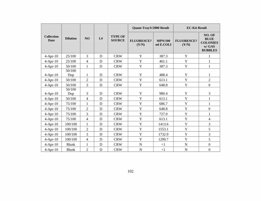
102
Collection
Date Dilution NO L#
TYPE OF
SOURCE
Quant-Tray®/2000 Result EC-Kit Result
FLUORESCE?
(Y/N)
MPN/100
ml E.COLI
FLUORESCE?
(Y/N)
NO. OF
BLUE
COLONIES
w/ GAS
BUBBLES
4-Apr-10 25/100 3 D CRW Y 387.3 Y 1
4-Apr-10 25/100 4 D CRW Y 461.1 Y 1
4-Apr-10 50/100 1 D CRW Y 387.3 Y 1
4-Apr-10 50/100
Dup 1 D CRW Y 488.4 Y 1
4-Apr-10 50/100 2 D CRW Y 613.1 Y 2
4-Apr-10 50/100 3 D CRW Y 648.8 Y 0
4-Apr-10 50/100
Dup 3 D CRW Y 980.4 Y 3
4-Apr-10 50/100 4 D CRW Y 613.1 Y 1
4-Apr-10 75/100 1 D CRW Y 686.7 Y 1
4-Apr-10 75/100 2 D CRW Y 648.8 Y 0
4-Apr-10 75/100 3 D CRW Y 727.0 Y 1
4-Apr-10 75/100 4 D CRW Y 613.1 Y 4
4-Apr-10 100/100 1 D CRW Y 1413.6 Y 3
4-Apr-10 100/100 2 D CRW Y 1553.1 Y 5
4-Apr-10 100/100 3 D CRW Y 1732.9 Y 3
4-Apr-10 100/100 4 D CRW Y 1299.7 Y 5
4-Apr-10 Blank 1 D CRW N <1 N 0
4-Apr-10 Blank 2 D CRW N <1 N 0

103
Appendix D: GPS Coordinates
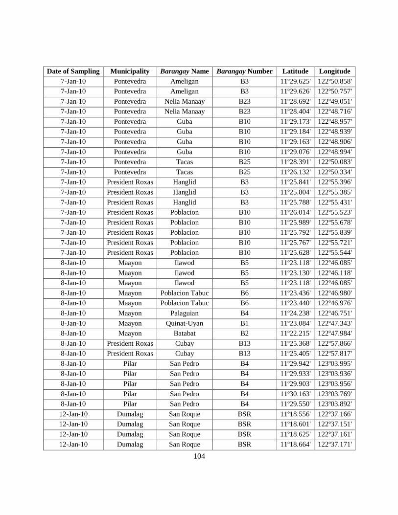
104
Date of Sampling Municipality Barangay Name Barangay Number Latitude Longitude
7-Jan-10 Pontevedra Ameligan B3 11º29.625' 122º50.858'
7-Jan-10 Pontevedra Ameligan B3 11º29.626' 122º50.757'
7-Jan-10 Pontevedra Nelia Manaay B23 11º28.692' 122º49.051'
7-Jan-10 Pontevedra Nelia Manaay B23 11º28.404' 122º48.716'
7-Jan-10 Pontevedra Guba B10 11º29.173' 122º48.957'
7-Jan-10 Pontevedra Guba B10 11º29.184' 122º48.939'
7-Jan-10 Pontevedra Guba B10 11º29.163' 122º48.906'
7-Jan-10 Pontevedra Guba B10 11º29.076' 122º48.994'
7-Jan-10 Pontevedra Tacas B25 11º28.391' 122º50.083'
7-Jan-10 Pontevedra Tacas B25 11º26.132' 122º50.334'
7-Jan-10 President Roxas Hanglid B3 11º25.841' 122º55.396'
7-Jan-10 President Roxas Hanglid B3 11º25.804' 122º55.385'
7-Jan-10 President Roxas Hanglid B3 11º25.788' 122º55.431'
7-Jan-10 President Roxas Poblacion B10 11º26.014' 122º55.523'
7-Jan-10 President Roxas Poblacion B10 11º25.989' 122º55.678'
7-Jan-10 President Roxas Poblacion B10 11º25.792' 122º55.839'
7-Jan-10 President Roxas Poblacion B10 11º25.767' 122º55.721'
7-Jan-10 President Roxas Poblacion B10 11º25.628' 122º55.544'
8-Jan-10 Maayon Ilawod B5 11º23.118' 122º46.085'
8-Jan-10 Maayon Ilawod B5 11º23.130' 122º46.118'
8-Jan-10 Maayon Ilawod B5 11º23.118' 122º46.085'
8-Jan-10 Maayon Poblacion Tabuc B6 11º23.436' 122º46.980'
8-Jan-10 Maayon Poblacion Tabuc B6 11º23.440' 122º46.976'
8-Jan-10 Maayon Palaguian B4 11º24.238' 122º46.751'
8-Jan-10 Maayon Quinat-Uyan B1 11º23.084' 122º47.343'
8-Jan-10 Maayon Batabat B2 11º22.215' 122º47.984'
8-Jan-10 President Roxas Cubay B13 11º25.368' 122º57.866'
8-Jan-10 President Roxas Cubay B13 11º25.405' 122º57.817'
8-Jan-10 Pilar San Pedro B4 11º29.942' 123º03.995'
8-Jan-10 Pilar San Pedro B4 11º29.933' 123º03.936'
8-Jan-10 Pilar San Pedro B4 11º29.903' 123º03.956'
8-Jan-10 Pilar San Pedro B4 11º30.163' 123º03.769'
8-Jan-10 Pilar San Pedro B4 11º29.550' 123º03.892'
12-Jan-10 Dumalag San Roque BSR 11º18.556' 122º37.166'
12-Jan-10 Dumalag San Roque BSR 11º18.601' 122º37.151'
12-Jan-10 Dumalag San Roque BSR 11º18.625' 122º37.161'
12-Jan-10 Dumalag San Roque BSR 11º18.664' 122º37.171'
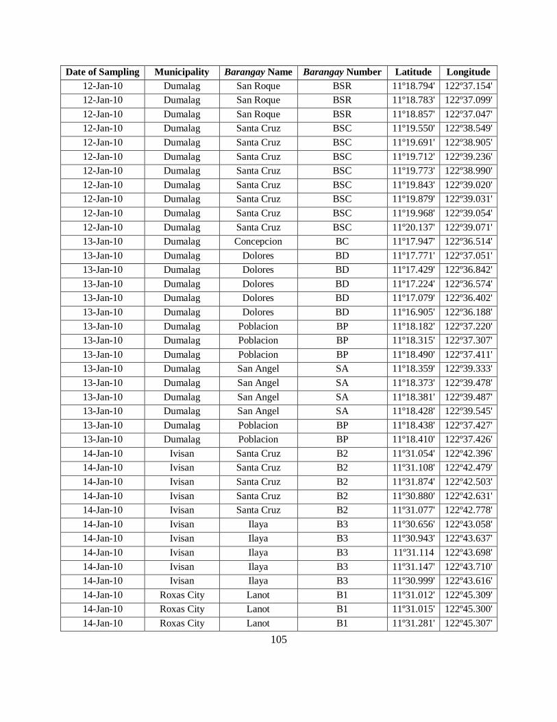
105
Date of Sampling Municipality Barangay Name Barangay Number Latitude Longitude
12-Jan-10 Dumalag San Roque BSR 11º18.794' 122º37.154'
12-Jan-10 Dumalag San Roque BSR 11º18.783' 122º37.099'
12-Jan-10 Dumalag San Roque BSR 11º18.857' 122º37.047'
12-Jan-10 Dumalag Santa Cruz BSC 11º19.550' 122º38.549'
12-Jan-10 Dumalag Santa Cruz BSC 11º19.691' 122º38.905'
12-Jan-10 Dumalag Santa Cruz BSC 11º19.712' 122º39.236'
12-Jan-10 Dumalag Santa Cruz BSC 11º19.773' 122º38.990'
12-Jan-10 Dumalag Santa Cruz BSC 11º19.843' 122º39.020'
12-Jan-10 Dumalag Santa Cruz BSC 11º19.879' 122º39.031'
12-Jan-10 Dumalag Santa Cruz BSC 11º19.968' 122º39.054'
12-Jan-10 Dumalag Santa Cruz BSC 11º20.137' 122º39.071'
13-Jan-10 Dumalag Concepcion BC 11º17.947' 122º36.514'
13-Jan-10 Dumalag Dolores BD 11º17.771' 122º37.051'
13-Jan-10 Dumalag Dolores BD 11º17.429' 122º36.842'
13-Jan-10 Dumalag Dolores BD 11º17.224' 122º36.574'
13-Jan-10 Dumalag Dolores BD 11º17.079' 122º36.402'
13-Jan-10 Dumalag Dolores BD 11º16.905' 122º36.188'
13-Jan-10 Dumalag Poblacion BP 11º18.182' 122º37.220'
13-Jan-10 Dumalag Poblacion BP 11º18.315' 122º37.307'
13-Jan-10 Dumalag Poblacion BP 11º18.490' 122º37.411'
13-Jan-10 Dumalag San Angel SA 11º18.359' 122º39.333'
13-Jan-10 Dumalag San Angel SA 11º18.373' 122º39.478'
13-Jan-10 Dumalag San Angel SA 11º18.381' 122º39.487'
13-Jan-10 Dumalag San Angel SA 11º18.428' 122º39.545'
13-Jan-10 Dumalag Poblacion BP 11º18.438' 122º37.427'
13-Jan-10 Dumalag Poblacion BP 11º18.410' 122º37.426'
14-Jan-10 Ivisan Santa Cruz B2 11º31.054' 122º42.396'
14-Jan-10 Ivisan Santa Cruz B2 11º31.108' 122º42.479'
14-Jan-10 Ivisan Santa Cruz B2 11º31.874' 122º42.503'
14-Jan-10 Ivisan Santa Cruz B2 11º30.880' 122º42.631'
14-Jan-10 Ivisan Santa Cruz B2 11º31.077' 122º42.778'
14-Jan-10 Ivisan Ilaya B3 11º30.656' 122º43.058'
14-Jan-10 Ivisan Ilaya B3 11º30.943' 122º43.637'
14-Jan-10 Ivisan Ilaya B3 11º31.114 122º43.698'
14-Jan-10 Ivisan Ilaya B3 11º31.147' 122º43.710'
14-Jan-10 Ivisan Ilaya B3 11º30.999' 122º43.616'
14-Jan-10 Roxas City Lanot B1 11º31.012' 122º45.309'
14-Jan-10 Roxas City Lanot B1 11º31.015' 122º45.300'
14-Jan-10 Roxas City Lanot B1 11º31.281' 122º45.307'
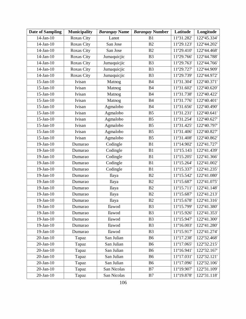
106
Date of Sampling Municipality Barangay Name Barangay Number Latitude Longitude
14-Jan-10 Roxas City Lanot B1 11º31.282' 122º45.334'
14-Jan-10 Roxas City San Jose B2 11º29.123' 122º44.202'
14-Jan-10 Roxas City San Jose B2 11º29.410' 122º44.468'
14-Jan-10 Roxas City Jumaquicjic B3 11º29.766' 122º44.788'
14-Jan-10 Roxas City Jumaquicjic B3 11º29.763' 122º44.766'
14-Jan-10 Roxas City Jumaquicjic B3 11º29.727' 122º44.909'
14-Jan-10 Roxas City Jumaquicjic B3 11º29.739' 122º44.972'
15-Jan-10 Ivisan Matnog B4 11º31.304' 122º40.371'
15-Jan-10 Ivisan Matnog B4 11º31.602' 122º40.620'
15-Jan-10 Ivisan Matnog B4 11º31.738' 122º40.422'
15-Jan-10 Ivisan Matnog B4 11º31.776' 122º40.401'
15-Jan-10 Ivisan Agmalobo B4 11º31.656' 122º40.490'
15-Jan-10 Ivisan Agmalobo B5 11º31.231' 122º40.641'
15-Jan-10 Ivisan Agmalobo B5 11º31.254' 122º40.627'
15-Jan-10 Ivisan Agmalobo B5 11º31.425' 122º40.797'
15-Jan-10 Ivisan Agmalobo B5 11º31.406' 122º40.827'
15-Jan-10 Ivisan Agmalobo B5 11º31.408' 122º40.862'
19-Jan-10 Dumarao Codingle B1 11º14.902' 122º41.727'
19-Jan-10 Dumarao Codingle B1 11º15.143 122º41.439'
19-Jan-10 Dumarao Codingle B1 11º15.205' 122º41.366'
19-Jan-10 Dumarao Codingle B1 11º15.264' 122º41.002'
19-Jan-10 Dumarao Codingle B1 11º15.337' 122º41.235'
19-Jan-10 Dumarao Ilaya B2 11º15.542' 122º41.080'
19-Jan-10 Dumarao Ilaya B2 11º15.687' 122º41.075'
19-Jan-10 Dumarao Ilaya B2 11º15.711' 122º41.148'
19-Jan-10 Dumarao Ilaya B2 11º15.687' 122º41.213'
19-Jan-10 Dumarao Ilaya B2 11º15.678' 122º41.316'
19-Jan-10 Dumarao Ilawod B3 11º15.799' 122º41.380'
19-Jan-10 Dumarao Ilawod B3 11º15.926' 122º41.353'
19-Jan-10 Dumarao Ilawod B3 11º15.947' 122º41.300'
19-Jan-10 Dumarao Ilawod B3 11º16.003' 122º41.280'
19-Jan-10 Dumarao Ilawod B3 11º15.917' 122º41.274'
20-Jan-10 Tapaz San Julian B6 11º17.238' 122º32.468'
20-Jan-10 Tapaz San Julian B6 11º17.065' 122º32.215'
20-Jan-10 Tapaz San Julian B6 11º16.941' 122º32.167'
20-Jan-10 Tapaz San Julian B6 11º17.031' 122º32.121'
20-Jan-10 Tapaz San Julian B6 11º17.096' 122º32.106'
20-Jan-10 Tapaz San Nicolas B7 11º19.907' 122º31.109'
20-Jan-10 Tapaz San Nicolas B7 11º19.878' 122º31.118'
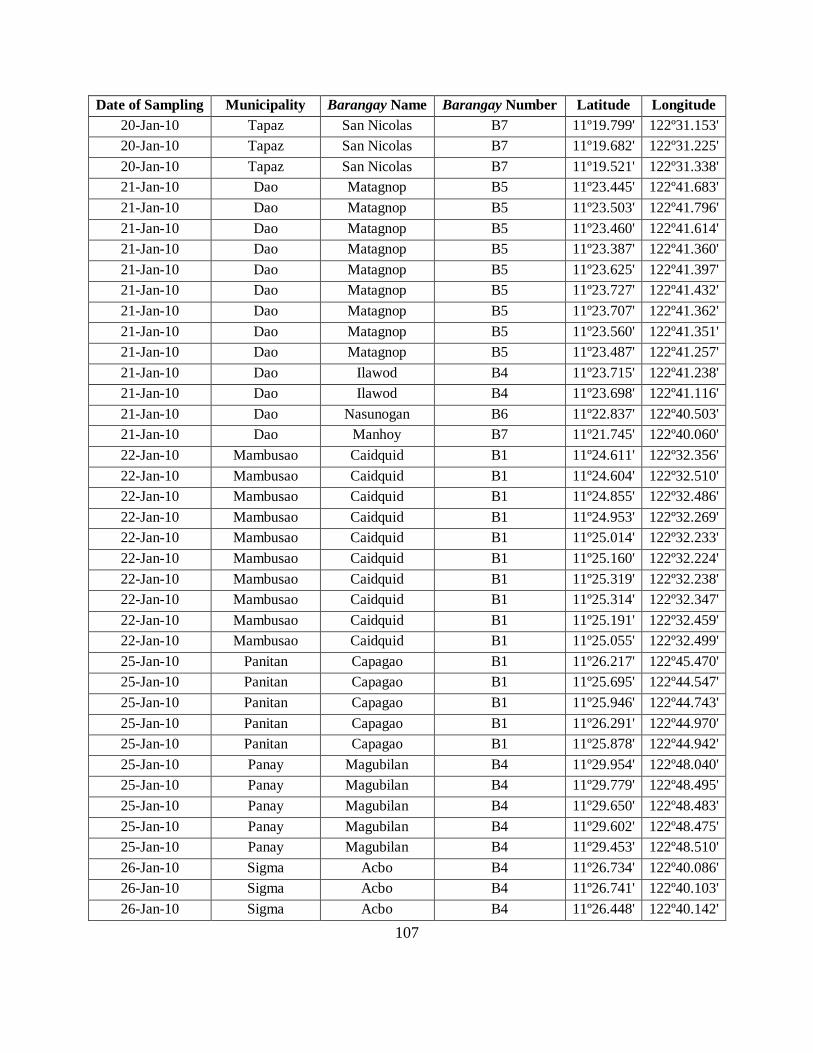
107
Date of Sampling Municipality Barangay Name Barangay Number Latitude Longitude
20-Jan-10 Tapaz San Nicolas B7 11º19.799' 122º31.153'
20-Jan-10 Tapaz San Nicolas B7 11º19.682' 122º31.225'
20-Jan-10 Tapaz San Nicolas B7 11º19.521' 122º31.338'
21-Jan-10 Dao Matagnop B5 11º23.445' 122º41.683'
21-Jan-10 Dao Matagnop B5 11º23.503' 122º41.796'
21-Jan-10 Dao Matagnop B5 11º23.460' 122º41.614'
21-Jan-10 Dao Matagnop B5 11º23.387' 122º41.360'
21-Jan-10 Dao Matagnop B5 11º23.625' 122º41.397'
21-Jan-10 Dao Matagnop B5 11º23.727' 122º41.432'
21-Jan-10 Dao Matagnop B5 11º23.707' 122º41.362'
21-Jan-10 Dao Matagnop B5 11º23.560' 122º41.351'
21-Jan-10 Dao Matagnop B5 11º23.487' 122º41.257'
21-Jan-10 Dao Ilawod B4 11º23.715' 122º41.238'
21-Jan-10 Dao Ilawod B4 11º23.698' 122º41.116'
21-Jan-10 Dao Nasunogan B6 11º22.837' 122º40.503'
21-Jan-10 Dao Manhoy B7 11º21.745' 122º40.060'
22-Jan-10 Mambusao Caidquid B1 11º24.611' 122º32.356'
22-Jan-10 Mambusao Caidquid B1 11º24.604' 122º32.510'
22-Jan-10 Mambusao Caidquid B1 11º24.855' 122º32.486'
22-Jan-10 Mambusao Caidquid B1 11º24.953' 122º32.269'
22-Jan-10 Mambusao Caidquid B1 11º25.014' 122º32.233'
22-Jan-10 Mambusao Caidquid B1 11º25.160' 122º32.224'
22-Jan-10 Mambusao Caidquid B1 11º25.319' 122º32.238'
22-Jan-10 Mambusao Caidquid B1 11º25.314' 122º32.347'
22-Jan-10 Mambusao Caidquid B1 11º25.191' 122º32.459'
22-Jan-10 Mambusao Caidquid B1 11º25.055' 122º32.499'
25-Jan-10 Panitan Capagao B1 11º26.217' 122º45.470'
25-Jan-10 Panitan Capagao B1 11º25.695' 122º44.547'
25-Jan-10 Panitan Capagao B1 11º25.946' 122º44.743'
25-Jan-10 Panitan Capagao B1 11º26.291' 122º44.970'
25-Jan-10 Panitan Capagao B1 11º25.878' 122º44.942'
25-Jan-10 Panay Magubilan B4 11º29.954' 122º48.040'
25-Jan-10 Panay Magubilan B4 11º29.779' 122º48.495'
25-Jan-10 Panay Magubilan B4 11º29.650' 122º48.483'
25-Jan-10 Panay Magubilan B4 11º29.602' 122º48.475'
25-Jan-10 Panay Magubilan B4 11º29.453' 122º48.510'
26-Jan-10 Sigma Acbo B4 11º26.734' 122º40.086'
26-Jan-10 Sigma Acbo B4 11º26.741' 122º40.103'
26-Jan-10 Sigma Acbo B4 11º26.448' 122º40.142'
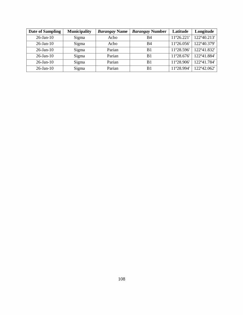
108
Date of Sampling Municipality Barangay Name Barangay Number Latitude Longitude
26-Jan-10 Sigma Acbo B4 11º26.221' 122º40.213'
26-Jan-10 Sigma Acbo B4 11º26.056' 122º40.379'
26-Jan-10 Sigma Parian B1 11º28.596' 122º41.832'
26-Jan-10 Sigma Parian B1 11º28.676' 122º41.884'
26-Jan-10 Sigma Parian B1 11º28.906' 122º41.784'
26-Jan-10 Sigma Parian B1 11º28.994' 122º42.062'

109
Appendix E: EC-Kit Instructions
Modified and Updated by Patty Chuang and Susan Murcott in May 2010
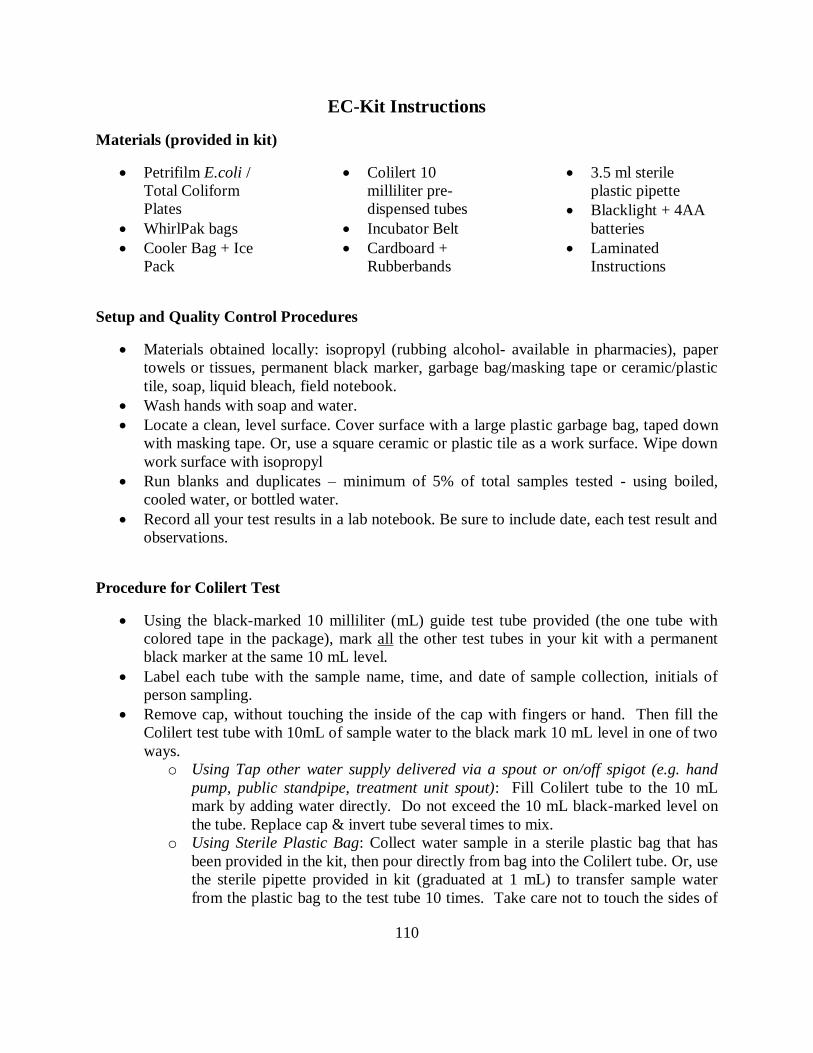
110
EC-Kit Instructions
Materials (provided in kit)
Petrifilm E.coli /
Total Coliform
Plates
WhirlPak bags
Cooler Bag + Ice
Pack
Colilert 10
milliliter pre-
dispensed tubes
Incubator Belt
Cardboard +
Rubberbands
3.5 ml sterile
plastic pipette
Blacklight + 4AA
batteries
Laminated
Instructions
Setup and Quality Control Procedures
Materials obtained locally: isopropyl (rubbing alcohol- available in pharmacies), paper
towels or tissues, permanent black marker, garbage bag/masking tape or ceramic/plastic
tile, soap, liquid bleach, field notebook.
Wash hands with soap and water.
Locate a clean, level surface. Cover surface with a large plastic garbage bag, taped down
with masking tape. Or, use a square ceramic or plastic tile as a work surface. Wipe down
work surface with isopropyl
Run blanks and duplicates – minimum of 5% of total samples tested - using boiled,
cooled water, or bottled water.
Record all your test results in a lab notebook. Be sure to include date, each test result and
observations.
Procedure for Colilert Test
Using the black-marked 10 milliliter (mL) guide test tube provided (the one tube with
colored tape in the package), mark all the other test tubes in your kit with a permanent
black marker at the same 10 mL level.
Label each tube with the sample name, time, and date of sample collection, initials of
person sampling.
Remove cap, without touching the inside of the cap with fingers or hand. Then fill the
Colilert test tube with 10mL of sample water to the black mark 10 mL level in one of two
ways.
o Using Tap other water supply delivered via a spout or on/off spigot (e.g. hand
pump, public standpipe, treatment unit spout): Fill Colilert tube to the 10 mL
mark by adding water directly. Do not exceed the 10 mL black-marked level on
the tube. Replace cap & invert tube several times to mix.
o Using Sterile Plastic Bag: Collect water sample in a sterile plastic bag that has
been provided in the kit, then pour directly from bag into the Colilert tube. Or, use
the sterile pipette provided in kit (graduated at 1 mL) to transfer sample water
from the plastic bag to the test tube 10 times. Take care not to touch the sides of
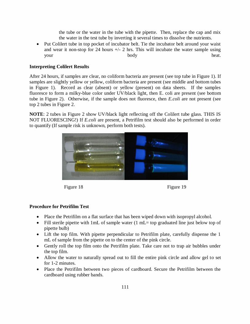
111
the tube or the water in the tube with the pipette. Then, replace the cap and mix
the water in the test tube by inverting it several times to dissolve the nutrients.
Put Colilert tube in top pocket of incubator belt. Tie the incubator belt around your waist
and wear it non-stop for 24 hours +/- 2 hrs. This will incubate the water sample using
your body heat.
Interpreting Colilert Results
After 24 hours, if samples are clear, no coliform bacteria are present (see top tube in Figure 1). If
samples are slightly yellow or yellow, coliform bacteria are present (see middle and bottom tubes
in Figure 1). Record as clear (absent) or yellow (present) on data sheets. If the samples
fluoresce to form a milky-blue color under UV/black light, then E. coli are present (see bottom
tube in Figure 2). Otherwise, if the sample does not fluoresce, then E.coli are not present (see
top 2 tubes in Figure 2.
NOTE: 2 tubes in Figure 2 show UV/black light reflecting off the Colilert tube glass. THIS IS
NOT FLUORESCING!) If E.coli are present, a Petrifilm test should also be performed in order
to quantify (If sample risk is unknown, perform both tests).
Figure 18 Figure 19
Procedure for Petrifilm Test
Place the Petrifilm on a flat surface that has been wiped down with isopropyl alcohol.
Fill sterile pipette with 1mL of sample water (1 mL= top graduated line just below top of
pipette bulb)
Lift the top film. With pipette perpendicular to Petrifilm plate, carefully dispense the 1
mL of sample from the pipette on to the center of the pink circle.
Gently roll the top film onto the Petrifilm plate. Take care not to trap air bubbles under
the top film.
Allow the water to naturally spread out to fill the entire pink circle and allow gel to set
for 1-2 minutes.
Place the Petrifilm between two pieces of cardboard. Secure the Petrifilm between the
cardboard using rubber bands.
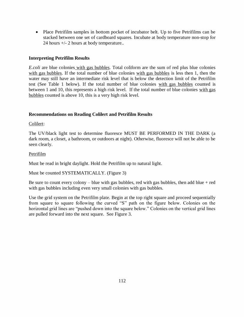
112
Place Petrifilm samples in bottom pocket of incubator belt. Up to five Petrifilms can be
stacked between one set of cardboard squares. Incubate at body temperature non-stop for
24 hours +/- 2 hours at body temperature..
Interpreting Petrifilm Results
E.coli are blue colonies with gas bubbles. Total coliform are the sum of red plus blue colonies
with gas bubbles. If the total number of blue colonies with gas bubbles is less then 1, then the
water may still have an intermediate risk level that is below the detection limit of the Petrifilm
test (See Table 1 below). If the total number of blue colonies with gas bubbles counted is
between 1 and 10, this represents a high risk level. If the total number of blue colonies with gas
bubbles counted is above 10, this is a very high risk level.
Recommendations on Reading Colilert and Petrifilm Results
Colilert:
The UV/black light test to determine fluoresce MUST BE PERFORMED IN THE DARK (a
dark room, a closet, a bathroom, or outdoors at night). Otherwise, fluoresce will not be able to be
seen clearly.
Petrifilm
Must be read in bright daylight. Hold the Petrifilm up to natural light.
Must be counted SYSTEMATICALLY. (Figure 3)
Be sure to count every colony – blue with gas bubbles, red with gas bubbles, then add blue + red
with gas bubbles including even very small colonies with gas bubbles.
Use the grid system on the Petrifilm plate. Begin at the top right square and proceed sequentially
from square to square following the curved “S” path on the figure below. Colonies on the
horizontal grid lines are “pushed down into the square below.” Colonies on the vertical grid lines
are pulled forward into the next square. See Figure 3.
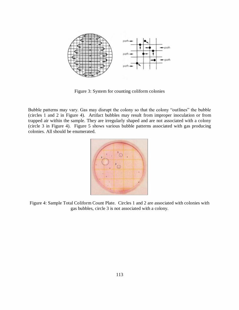
113
Figure 3: System for counting coliform colonies
Bubble patterns may vary. Gas may disrupt the colony so that the colony “outlines” the bubble
(circles 1 and 2 in Figure 4). Artifact bubbles may result from improper inoculation or from
trapped air within the sample. They are irregularly shaped and are not associated with a colony
(circle 3 in Figure 4). Figure 5 shows various bubble patterns associated with gas producing
colonies. All should be enumerated.
Figure 4: Sample Total Coliform Count Plate. Circles 1 and 2 are associated with colonies with
gas bubbles, circle 3 is not associated with a colony.
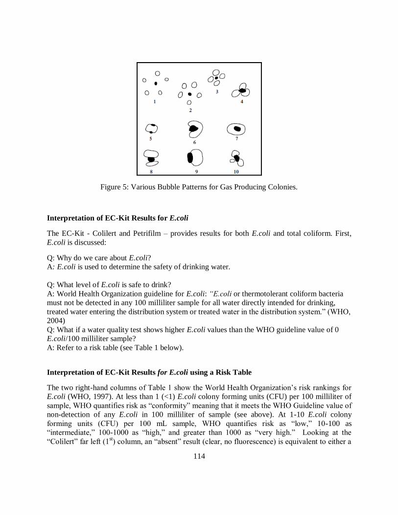
114
Figure 5: Various Bubble Patterns for Gas Producing Colonies.
Interpretation of EC-Kit Results for E.coli
The EC-Kit - Colilert and Petrifilm – provides results for both E.coli and total coliform. First,
E.coli is discussed:
Q: Why do we care about E.coli?
A: E.coli is used to determine the safety of drinking water.
Q: What level of E.coli is safe to drink?
A: World Health Organization guideline for E.coli: “E.coli or thermotolerant coliform bacteria
must not be detected in any 100 milliliter sample for all water directly intended for drinking,
treated water entering the distribution system or treated water in the distribution system.” (WHO,
2004)
Q: What if a water quality test shows higher E.coli values than the WHO guideline value of 0
E.coli/100 milliliter sample?
A: Refer to a risk table (see Table 1 below).
Interpretation of EC-Kit Results for E.coli using a Risk Table
The two right-hand columns of Table 1 show the World Health Organization’s risk rankings for
E.coli (WHO, 1997). At less than 1 (<1) E.coli colony forming units (CFU) per 100 milliliter of
sample, WHO quantifies risk as “conformity” meaning that it meets the WHO Guideline value of
non-detection of any E.coli in 100 milliliter of sample (see above). At 1-10 E.coli colony
forming units (CFU) per 100 mL sample, WHO quantifies risk as “low,” 10-100 as
“intermediate,” 100-1000 as “high,” and greater than 1000 as “very high.” Looking at the
“Colilert” far left (1st) column, an “absent” result (clear, no fluorescence) is equivalent to either a
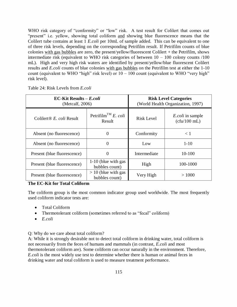
115
WHO risk category of “conformity” or “low” risk. A test result for Colilert that comes out
“present” i.e. yellow, showing total coliform and showing blue fluorescence means that the
Colilert tube contains at least 1 E.coli per 10mL of sample added. This can be equivalent to one
of three risk levels, depending on the corresponding Petrifilm result. If Petrifilm counts of blue
colonies with gas bubbles are zero, the present/yellow/fluorescent Colilert + the Petrifilm, shows
intermediate risk (equivalent to WHO risk categories of between 10 – 100 colony counts /100
mL). High and very high risk waters are identified by present/yellow/blue fluorescent Colilert
results and E.coli counts of blue colonies with gas bubbles on the Petrifilm test at either the 1-10
count (equivalent to WHO “high” risk level) or 10 – 100 count (equivalent to WHO “very high”
risk level).
Table 24: Risk Levels from E.coli
EC-Kit Results – E.coli
(Metcalf, 2006)
Risk Level Categories
(World Health Organization, 1997)
Colilert® E. coli Result Petrifilm
TM E. coli
Result Risk Level
E.coli in sample
(cfu/100 mL)
Absent (no fluorescence) 0 Conformity < 1
Absent (no fluorescence) 0 Low 1-10
Present (blue fluorescence) 0 Intermediate 10-100
Present (blue fluorescence) 1-10 (blue with gas
bubbles count) High 100-1000
Present (blue fluorescence) > 10 (blue with gas
bubbles count) Very High > 1000
The EC-Kit for Total Coliform
The coliform group is the most common indicator group used worldwide. The most frequently
used coliform indicator tests are:
Total Coliform
Thermotolerant coliform (sometimes referred to as “fecal” coliform)
E.coli
Q: Why do we care about total coliform?
A: While it is strongly desirable not to detect total coliform in drinking water, total coliform is
not necessarily from the feces of humans and mammals (in contrast, E.coli and most
thermotolerant coliform are). Some coliform can occur naturally in the environment. Therefore,
E.coli is the most widely use test to determine whether there is human or animal feces in
drinking water and total coliform is used to measure treatment performance.
116
Q: How is treatment performance measured?
A: Treatment performance is measured by sampling and running EC-Kit tests on at least two
samples from a treatment system. The treatment system can be of any scale: large centralized
treatment, community treatment or household treatment. The first sample one should collect is of
the influent water – the water that supplies the treatment system. The second sample is of the
treated water. By comparing the before treatment and after treatment samples, one can determine
a percentage removal efficiency of the treatment system. This helps determine if the treatment
system is performing effectively or not.
Interpretation of EC-Kit Results for Total Coliform
Total coliform are the sum of red colonies with gas bubbles plus blue colonies with gas bubbles
in the Petrifilm test. Interpret the total coliform counts using Table 2.
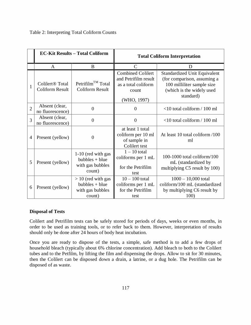
117
Table 2: Interpreting Total Coliform Counts
EC-Kit Results – Total Coliform
Total Coliform Interpretation
A B C D
1 Colilert® Total
Coliform Result
PetrifilmTM
Total
Coliform Result
Combined Colilert
and Petrifilm result
as a total coliform
count
(WHO, 1997)
Standardized Unit Equivalent
(for comparison, assuming a
100 milliliter sample size
(which is the widely used
standard)
2 Absent (clear,
no fluorescence) 0 0 <10 total coliform / 100 ml
3 Absent (clear,
no fluorescence) 0 0 <10 total coliform / 100 ml
4 Present (yellow) 0
at least 1 total
coliform per 10 ml
of sample in
Colilert test
At least 10 total coliform /100
ml
5 Present (yellow)
1-10 (red with gas
bubbles + blue
with gas bubbles
count)
1 – 10 total
coliforms per 1 mL
for the Petrifilm
test
100-1000 total coliform/100
mL (standardized by
multiplying C5 result by 100)
6 Present (yellow)
> 10 (red with gas
bubbles + blue
with gas bubbles
count)
10 – 100 total
coliforms per 1 mL
for the Petrifilm
test
1000 – 10,000 total
coliform/100 mL (standardized
by multiplying C6 result by
100)
Disposal of Tests
Colilert and Petrifilm tests can be safely stored for periods of days, weeks or even months, in
order to be used as training tools, or to refer back to them. However, interpretation of results
should only be done after 24 hours of body heat incubation.
Once you are ready to dispose of the tests, a simple, safe method is to add a few drops of
household bleach (typically about 6% chlorine concentration). Add bleach to both to the Colilert
tubes and to the Petfilm, by lifting the film and dispensing the drops. Allow to sit for 30 minutes,
then the Colilert can be disposed down a drain, a latrine, or a dug hole. The Petrifilm can be
disposed of as waste.