Embed Size (px)
Citation preview
IJRRAS 23 (2) ● May 2015 www.arpapress.com/Volumes/Vol23Issue2/IJRRAS_23_2_04.pdf
107
COMPARISON OF DIFFERENT NUMERICAL TECHNIQUES FOR THE
DEVELOPMENT OF A SIMULATOR OF SURFACTANT ASSISTED
ENHANCED OIL RECOVERY PROCESS
Kamilu Folorunsho Oyedeko1 & Alfred Akpoveta Susu2
1Department of Chemical & Polymer Engineering, Lagos State University, Epe, Lagos, Nigeria 2Department of Chemical Engineering, University of Lagos, Lagos, Nigeria
E-mail:[email protected]; [email protected]
ABSTRACT
In this work, a simulator is designed for enhanced oil recovery process for surfactant assisted water flooding. The
system being investigated consists of three components (petroleum, water and surfactant) and two-phases (aqueous
and oleic). The model equations are characterized by a system of non-linear, partial, differential equations: the
continuity equation for the transport of each component, Darcy’s equation for the flow of each phase and algebraic
equations. The simulator incorporates first order effects, with scope to accommodate two or three dimensions, two
fluid phases and one adsorbent phase and four other components. The numerical methods used in the solution of
the model equations are the orthogonal collocation, finite difference, and coherence theory techniques. Matlab
computer programs were used for the numerical solution of the model equations. The results of the orthogonal
collocation solution were compared with those of finite difference and coherence solutions. The results indicate
that the concentration of surfactants for orthogonal collocation show more features than the predictions of the
coherence solutions and the finite difference, offering more opportunities for further understanding of the physical
nature of the complex problem. Also, comparison of the orthogonal collocation solution with computations based
on finite difference and coherence theory methods offers possible explanation for the observed differences
especially between the methods and the two different reservoirs they represent.
Keywords: Simulator Design; Multidimensional, Multiphase and Multicomponent system; Surfactant Flooding;
Finite Difference Method; Orthogonal Collocation Technique; Coherence Theory Method.
1. INTRODUCTION
The depleting world oil reserve can be conservatively managed through the use of tertiary production techniques
known as Enhanced Oil Recovery procedures. Although production capacity can be enhanced through the primary
and secondary recovery methods, bringing new fields online is very expensive and recovery from existing fields by
conventional methods will not fully provide the necessary relief for global oil demand.
On an average, only about a third of the original oil in place can be recovered by the primary and secondary
methods. The rest of the oil is trapped in reservoir pores due to surface and interfacial forces. This trapped oil can be
recovered by reducing the capillary forces that prevent the oil from flowing within the pores of reservoir rock and
into the well bores. Due to high oil prices and declining production in many regions around the globe, the possible
application of advance technologies for further oil recovery, called “Enhanced Oil Recovery“(EOR) has become
more attractive. The technology of EOR involves the injection of a fluid or fluids or materials into a reservoir to
supplement the natural energy present in a reservoir, where the injected fluids interact with the reservoir
rock/oil/brine system to create favourable conditions for maximum oil recovery. Surfactants are injected for this
purpose to decrease the interfacial tension between oil and water in order to mobilize the oil trapped after secondary
recovery by water flooding.
In a surfactant flood, a multi-component multiphase system is involved. The theory of multi-component, multiphase
flow has been presented by several authors. The surfactant flooding is a form of chemical flooding process and is
represented by a system of nonlinear, partial differential equations: the continuity equation for the transport of the
components and Darcy’s equation for the phase flow.
IJRRAS 23 (2) ● May 2015 Oyedeko & Susu ● Simulator for Enhanced Oil Recovery Process
108
Systems of coupled, first-order, nonlinear hyperbolic partial differential equations (p.d.e.s) govern the transient
evolution of a chemical flooding process for enhanced recovery. The method of characteristics (MOC) provides a
way in which such systems of hyperbolic p.d.e.s can be solved by converting them to an equivalent system of
ordinary differential equations. In fact, the MOC provides a similar framework for algorithm development to the
coherence approach adopted here. In some cases, the characteristic solution has been used to track the flood-front in
two-dimensional reservoir problems1. While the approach proposed by Ewing et al.2, combines the characteristic
method with a finite element approach. Zheng 3 has used the MOC and an adjustable number of moving particles to
track three-dimensional solute fronts in groundwater systems; adjusting the number of particles serves to maintain
an accurate material balance and save computational time. This front-tracking approach has been used in the present
work to trace the movement of coherent waves, of both the diffuse and shock variety.
The concept of coherence was extended to general EOR processes4,5, including alkaline flooding6, convectional
surfactant flooding7, the effects of cation-exchange on surfactant-polymer flooding8. Refinements to the theory also
allowed for equilibrium reaction to occur, such as precipitation-dissolution9,10 and micelle formation11. Helset and
Lake12 have used simple wave theory (essentially identical to coherence theory) to study the one dimensional, three
phase secondary migration of hydrocarbons from a source rock into possible reservoirs. Most recently, the theory of
coherence has been applied successfully to the analysis of the transport of volatile compounds in porous media in
the presence of a trapped gas phase13.
At the simple level, the results of simulation using the principle of coherence are analogous to the Buckley-Leverett
theory for waterflooding, the latter being evident in the work of Patton et al.14 for polymer flooding, Fayers and
Perrine15 for dilute surfactant flooding, Claridge and Bondor16 for carbonated water flooding, and Larson17 and
Hirasaki7 for miscible and immiscible surfactant flooding, respectively, Pope, et al.18 for isothermal, multiphase,
multicomponent fluid flow in permeable media and Hankins and Harwell19 for case studies in the feasibility of
sweep improvement in surfactant-assisted water flooding.
High oil prices and declining production in many regions around the globe make enhanced oil recovery (EOR)
increasingly attractive for investigators. As evident in the work of Siggel.et al20 for a new class of viscoelastic
surfactants for EOR, Xu and Lu 21 for microbially enhanced oil recovery at simulated reservoir conditions by use of
engineered bacteria, Leach and Mason22 for co-optimization of enhanced oil recovery and carbon sequestration,
Harwell23 for development of improved surfactants and EOR methods for small operators and many others.
The present work describes the development of a simulator for an Enhanced Oil Recovery process for surfactant
assisted water flooding by applying different mathematical methods for solution of the model transport equations.
The approach adopted here involves the use of different mathematical techniques, namely, orthogonal collocation
method, finite difference and coherence theory methods for the development and solution of the relevant nonlinear
partial differential equations. The different mathematical techniques are to be utilized to identify a particular type of
physical behaviour and enable the understanding of the involved propagation phenomena. In particular, the
techniques will be utilized for the prediction of what happens in EOR processes and possibly indicate how the
reduction of the complexity of the problem.
The approach is multidimensional in that it involved at least three independent variables and the introduction of the
concept of partial coherence which mean that the various composition path spaces required to map the composition
routes of the system are at most two dimensional, allowing for a great simplification in complexity.
2. METHODOLOGY
This work considered solving multidimensional, multicomponent, multiphase flow problem associated with
enhanced oil recovery process in petroleum engineering. The process of interest involves the injection of surfactant
of different concentrations and pore volume to displace oil from the reservoir.
The methodology illustrates the steps utilized in executing the project using the developed mathematical models to
describe the physics of reservoir depletion and fluid flow in which the areal distribution of fluids in the reservoir
IJRRAS 23 (2) ● May 2015 Oyedeko & Susu ● Simulator for Enhanced Oil Recovery Process
109
resulting from a flood is one of its main aims. The system is for two or three dimensions, two fluid phases (aqueous,
oleic) and one adsorbent phase, four components (oil, water, surfactants 1 and 2).
The reservoir may be divided into discrete grid blocks which may each be characterized by having different
reservoir properties. The flow of fluids from a block is governed by the principle of mass conservation coupled with
Darcy’s law. The simultaneous flow of oil, gas, and water, in three dimensions and the effects of natural water
influx, fluid compressibility, mass transfer between gas and liquid phases and the variation of such parameters as
porosity and permeability, as functions of pressure are then modelled.
The model is developed from the basic law of conservation of mass24. The developed partial differential equation is
converted to ordinary differential equation using coherent, finite difference and orthogonal collocation methods.
The finite difference method is a technique that converts partial differential equations into a system of linear
equations. There are essentially three finite difference techniques. The explicit finite difference method converts the
partial differential equations into an algebraic equation which can be solved by stepping forward (forward
difference), backward (backward difference) or centrally (central difference).
The orthogonal collocation method converts partial differential equations into a system of ordinary differential
equations using the lagrangian polynomial method. This set of ordinary differential equations generated is then
solved with appropriate numerical technique such as Runge Kutta.
The coherent theory method combines the forward finite difference method with Runge Kutta technique to solve
partial differential equations.
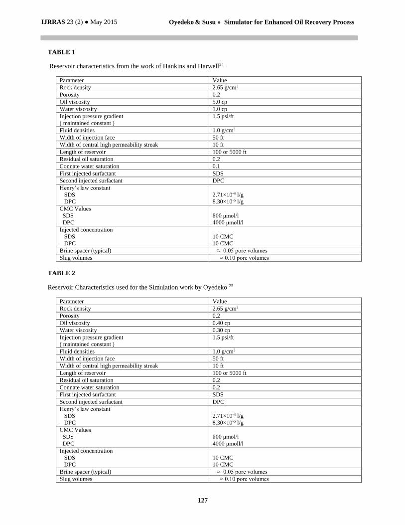
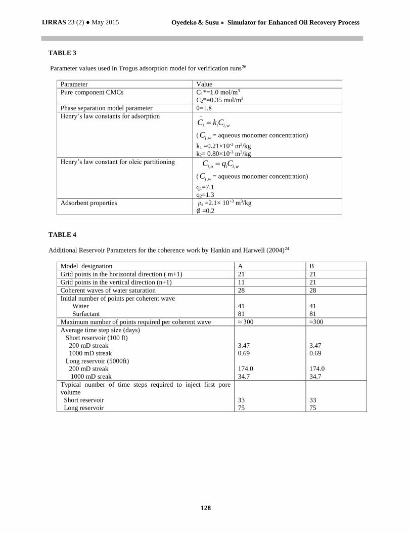
In the various solutions, several parameters are needed. The rock and fluid properties such as density, porosity,
viscosity, oil and water etc, and other parameters are provided in Tables 1, 2, 3 and 4. Table 1 is the Reservoir
characteristics from the work of Hankins and Harwell24. Table 2 is the Reservoir Characteristics used for the
simulation work by Oyedeko25. Parameter values used in Trogus adsorption model for verification runs is shown in
Table 3 while Table 4 presents additional reservoir parameters for the coherence work by Hankins and Harwell.24
In the present instance, in considering the more general form of the multiphase-multicomponent problem, the
explicit Runge-Kutta method is chosen to solve the problem. The motivation for this explicit method is its simplicity
and computational efficiency with the possibility of reducing truncation errors over those required for other
methods.
The model encompasses two fluid phases (aqueous and oleic), one adsorbent phase (rock), and four components (oil,
water, surfactants 1 and 2). The oil is displaced by water flooding. In-situ interaction of surfactant slugs may occur,
with consequent phase separation and local permeability reduction. The model accommodates two (or three)
physical dimensions, and an arbitrary, nonisotropic description of absolute permeability variation and porosity.
For most of the simulated cases in the work of Harkins and Harwell24, the reservoir consisted of a rectangular
composite of horizontal oil bearing strata, sandwiched above and below by two impervious rocks. Oil is produced
from the reservoir by means of water injection at one end and a production well at the other. Data for the
hypothetical reservoir simulated in Hankins and Harwell24 are given in Table1 and the governing model equation is
as shown by:
, , ,1 1,2
i w i w i wiw x w y w i
C C CCS v f v f r i
t t x y
(1)
IJRRAS 23 (2) ● May 2015 Oyedeko & Susu ● Simulator for Enhanced Oil Recovery Process
110
The term ir represents the rate of loss of surfactant due to precipitation: for a one-to-one reaction stoichiometry,
1 2r r . Since reaction occurs instantaneously at a sharp interface, this term may be ignored away from the singular
region of the interface.
It is possible to approximate the adsorption isotherm of a pure surfactant on a mineral oxide by use of a simple
model. At low concentration, the adsorption obeys Henry’s law, while above the critical micelle concentration
(CMC) the total adsorption remains constant. The Trogus adsorption model11,26 is used in this work.
2.1 Application of Coherence Theory to Solution of Model Equations
The material balance equations, Eqn. 1 (in the absence of ir ), are first order, homogeneous, nonlinear hyperbolic
equations. Their solution will be attempted by means of the theory of coherence. The results presented here are
general, and not restricted to assumptions regarding equilibrium relationships, fractional flow relationships, etc.
The concept of Coherence identifies the state which a dynamic, multi-component system strives to attain. The state
of “coherence” requires all dependent variables at any given point in space and time to have the same wave velocity,
giving rise to “a coherent” wave with no relative shift in the profiles of the variables. It has been established
mathematically by Helfferich27that an arbitrary starting variation of dependent variables, if embedded between
sufficiently large regions of constant state, is resolved into coherent waves, which become separated by new regions
of constant state.
2.2.1 Oleic Partitioning
The model developed and expressed in Eqn.1 may be generalized by allowing
surfactants to partition into the oleic phase. In general, , , 1, , 2,i o i o w wC C C C this leads to:
,, , , , , ,
1i wi w i o i w i w i o i o
w o x w y w x o y o i
C C C C C CCS S v f v f v f v f r
t t t x y x x
(2)
Leading to the matrix equation:
1,11 11 12 12 12
2,21 21 21 22 22 22
0ww o ii w o o o
wo o w o w o
dCS S p m f f p S p m f p
dCS p m f p S S p m f f p
(3)
where
,
,
,
i o
i j
j w
Cp
C
, 1o wf f , 1o wS S
2.3 Application of Finite Difference to Solution of Model Equations
First-order, finite-difference expressions for the spatial derivatives were substituted into the hyperbolic
chromatographic transport equations (Eq. 1), yielding 2 x m coupled ordinary differential equations which may then
be integrated simultaneously (also known as the ‘numerical method of lines’).
IJRRAS 23 (2) ● May 2015 Oyedeko & Susu ● Simulator for Enhanced Oil Recovery Process
111
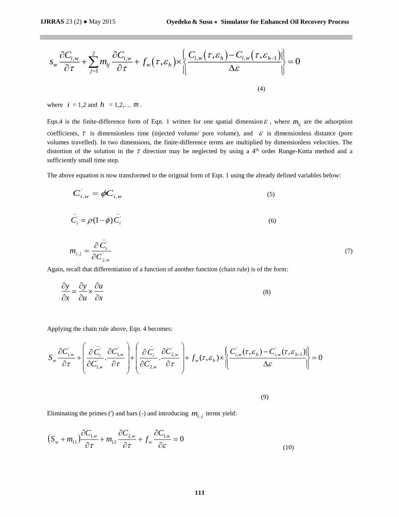
(4)
where i = 1,2 and h = 1,2,. .. m .
Eqn.4 is the finite-difference form of Eqn. 1 written for one spatial dimension , where ijm are the adsorption
coefficients, is dimensionless time (injected volume/ pore volume), and is dimensionless distance (pore
volumes travelled). In two dimensions, the finite-difference terms are multiplied by dimensionless velocities. The
distortion of the solution in the direction may be neglected by using a 4th order Runge-Kutta method and a
sufficiently small time step.
The above equation is now transformed to the original form of Eqn. 1 using the already defined variables below:
wiwi CC ,
'
, (5)
_'
_' )1( ii CC (6)
'
,
_'
,
wj
iji
C
Cm
(7)
Again, recall that differentiation of a function of another function (chain rule) is of the form:
x
u
u
y
x
y
(8)
Applying the chain rule above, Eqn. 4 becomes:
0),(),(
),(..1
'
,
'
,
'
,2
'
,2
_''
,1
'
,1
_''
,
hwihwi
hw
w
w
iw
w
iwi
w
CCf
C
C
CC
C
CCS
(9)
Eliminating the primes (') and bars (-) and introducing jim , terms yield:
0,1,2
12
,1
11
w
w
ww
w
Cf
Cm
CmS
(10)
2
, , 1, ,
1
, ,, 0
i w i wh hi w i ww ij w h
j
C CC Cs m f
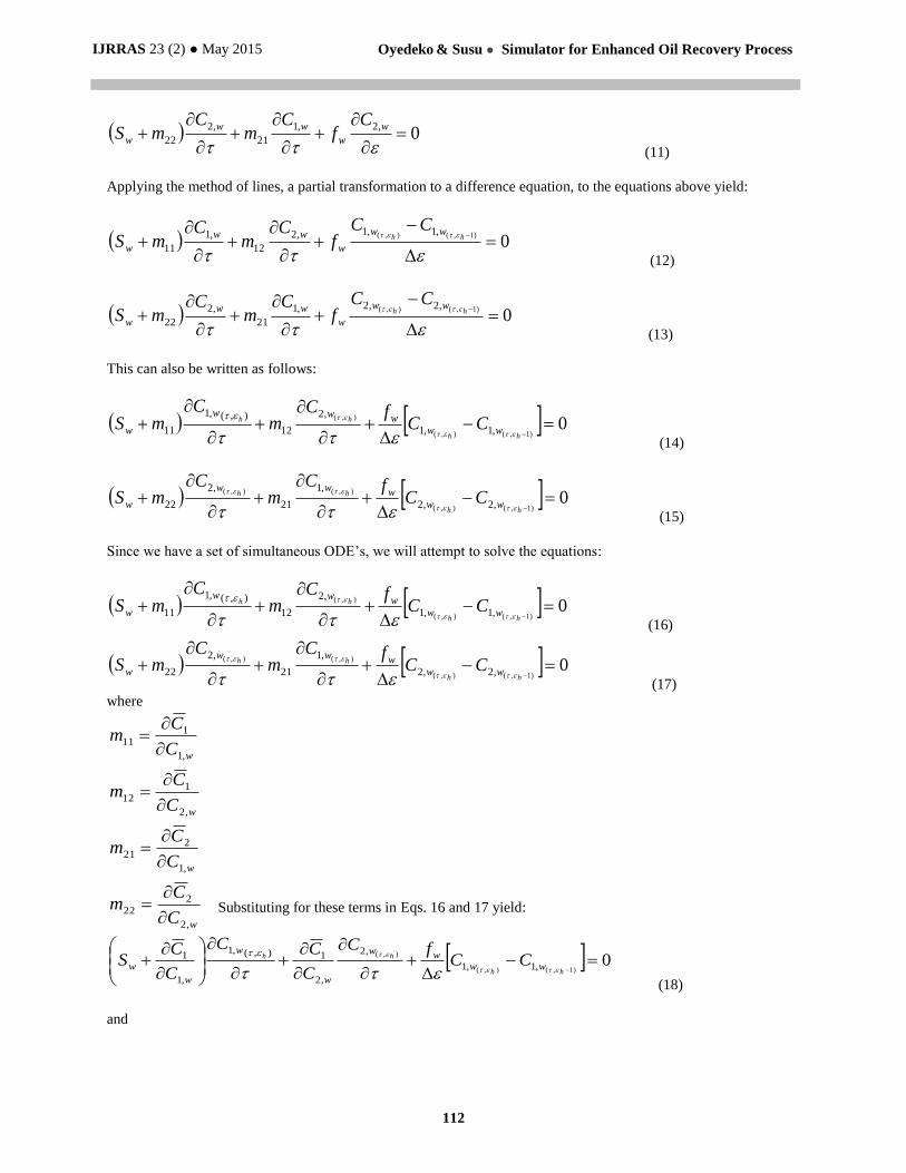
IJRRAS 23 (2) ● May 2015 Oyedeko & Susu ● Simulator for Enhanced Oil Recovery Process
112
0,2,1
21
,2
22
w
w
ww
w
Cf
Cm
CmS
(11)
Applying the method of lines, a partial transformation to a difference equation, to the equations above yield:
0)1,(),( ,1,1,2
12
,1
11
hhww
w
ww
w
CCf
Cm
CmS
(12)
0)1,(),( ,2,2,1
21
,2
22
hhww
w
ww
w
CCf
Cm
CmS
(13)
This can also be written as follows:
0)1,(),(
),(
,1,1
,2
12
),(,1
11
hh
hh
wwwww
w CCfC
mC
mS
(14)
0)1,(),(
),(),(
,2,2
,1
21
,2
22
hh
hh
wwwww
w CCfC
mC
mS
(15)
Since we have a set of simultaneous ODE’s, we will attempt to solve the equations:
0)1,(),(
),(
,1,1
,2
12
),(,1
11
hh
hh
wwwww
w CCfC
mC
mS
(16)
0)1,(),(
),(),(
,2,2
,1
21
,2
22
hh
hh
wwwww
w CCfC
mC
mS
(17)
where
Substituting for these terms in Eqs. 16 and 17 yield:
0)1,(),(
),(
,1,1
,2
,2
1),(,1
,1
1
hh
hh
wwww
w
w
w
w CCfC
C
CC
C
CS
(18)
and
w
w
w
w
C
Cm
C
Cm
C
Cm
C
Cm
,2
222
,1
221
,2
112
,1
111
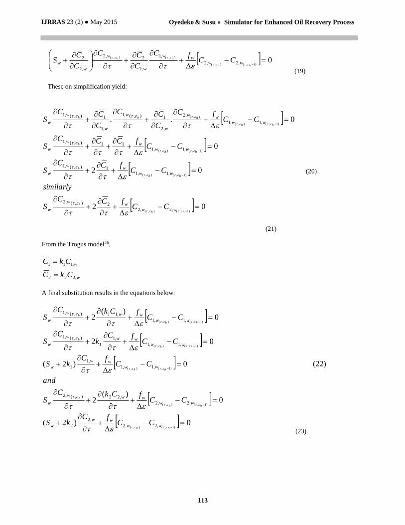
IJRRAS 23 (2) ● May 2015 Oyedeko & Susu ● Simulator for Enhanced Oil Recovery Process
113
0)1,(),(
),(),(
,2,2
,1
,1
2,2
,2
2
hh
hh
wwww
w
w
w
w CCfC
C
CC
C
CS
(19)
These on simplification yield:
02
02
0
0..
)1,(),(
)1,(),(
)1,(),(
)1,(),(
),(
,2,22),(,2
,1,11),(,1
,1,111),(,1
,1,1
,2
,2
1),(,1
,1
1),(,1
hh
h
hh
h
hh
h
hh
hhh
www
w
w
www
w
w
www
w
w
wwww
w
w
w
w
w
CCfCC
S
similarly
CCfCC
S
CCfCCC
S
CCfC
C
CC
C
CCS
(20)
(21)
From the Trogus model26,
w
w
CkC
CkC
,222
,111
A final substitution results in the equations below.
0)2(
0)(
2
0)2(
02
0)(
2
)1,(),(
)1,(),(
)1,(),(
)1,(),(
)1,(),(
,2,2
,2
2
,2,2
,22),(,2
,1,1
,1
1
,1,1
,1
1
),(,1
,1,1
,11),(,1
hh
hh
h
hh
hh
h
hh
h
wwww
w
wwwww
w
wwww
w
wwwww
w
wwwww
w
CCfC
kS
CCfCkC
S
and
CCfC
kS
CCfC
kC
S
CCfCkC
S
(23)
(22)
IJRRAS 23 (2) ● May 2015 Oyedeko & Susu ● Simulator for Enhanced Oil Recovery Process
114
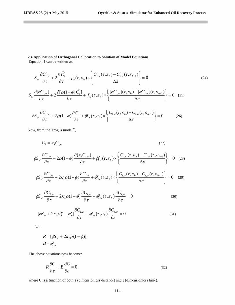
2.4 Application of Orthogonal Collocation to Solution of Model Equations
Equation 1 can be written as:
0),(),(
),(21
'
,
'
,
_''
,
hwihwi
hwiwi
w
CCf
CCS (24)
0),]([),]([
),(])1([
2][ 1,,
_
,
hwihwi
hwiwi
w
CCf
CCS
(25)
0),(),(
),()1(21,,
_
,
hwihwi
hwiwi
w
CCf
CCS (26)
Now, from the Trogus model26,
wiii CC ,
_
(27)
0),(),(
),()(
)1(21,,,,
hwihwi
hw
wiiwi
w
CCf
CCS (28)
0),(),(
),()1(21,,,,
hwihwi
hw
wi
i
wi
w
CCf
CCS (29)
0),()1(2,,,
wi
hw
wi
i
wi
w
Cf
CCS (30)
0),()]1(2[,,
wi
hw
wi
iw
Cf
CS (31)
Let
w
iw
fB
SR
)]1(2[
The above equations now become:
0
CB
CR (32)
where C is a function of both ԑ (dimensionless distance) and τ (dimensionless time).
IJRRAS 23 (2) ● May 2015 Oyedeko & Susu ● Simulator for Enhanced Oil Recovery Process
115
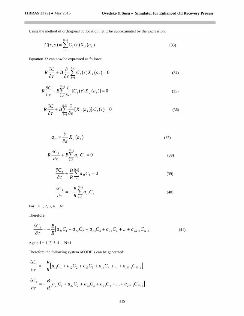
Using the method of orthogonal collocation, let C be approximated by the expression:
1
1
)()(),(N
I
IJI XCC (33)
Equation 32 can now be expressed as follows:
0)()(1
1
N
I
IJI XCBC
R
(34)
0])()([1
1
N
I
IJI XCBC
R
(35)
0)(].)([1
1
I
N
I
IJ CXBC
R (36)
)( IJJI Xa
(37)
01
1
I
N
I
JI
J CaBC
R
(38)
01
1
I
N
I
JI
J CaR
BC
(39)
I
N
I
JI
J CaR
BC
1
1 (40)
For I = 1, 2, 3, 4… N+1
Therefore,
1144332211 ...
NJNJJJJ
J CaCaCaCaCaR
BC
(41)
Again J = 1, 2, 3, 4… N+1
Therefore the following system of ODE’s can be generated:
111414313212111
1 ...
NN CaCaCaCaCa
R
BC
112424323222121
2 ...
NN CaCaCaCaCa
R
BC
IJRRAS 23 (2) ● May 2015 Oyedeko & Susu ● Simulator for Enhanced Oil Recovery Process
116
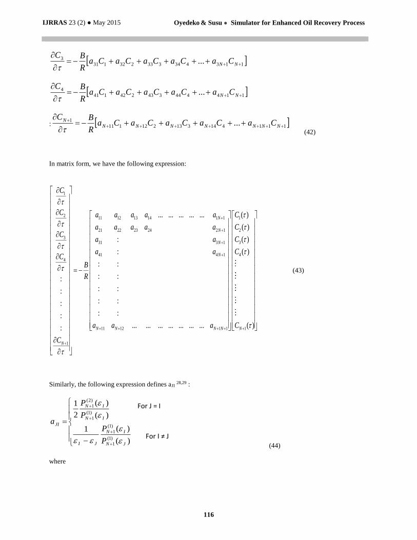
113434333232131
3 ...
NN CaCaCaCaCa
R
BC
114444343242141
4 ...
NN CaCaCaCaCa
R
BC
: 111414313212111
1 ...
NNNNNNN
N CaCaCaCaCaR
BC
(42)
In matrix form, we have the following expression:
1
211 12 13 14 1 1
21 22 23 24 2 1
331 3 1
41 4 14
11 12 1 1
1
... ... ... ... ...
:
:
: :
: ::
: ::
: ::
: ::
... ... ... ... ... ... ...:
N
N
N
N
N N N N
N
C
C a a a a a
a a a a aC
a a
a aC
B
R
a a a
C
1
2
3
4
1
( )
( )
( )
( )
( )N
C
C
C
C
C
(43)
Similarly, the following expression defines aJI 28,29 :
)(
)(1
)(
)(
2
1
)1(
1
)1(
1
)1(
1
)2(
1
JN
IN
JI
IN
IN
JI
P
P
P
P
a
(44)
where
For J = I
For I ≠ J
IJRRAS 23 (2) ● May 2015 Oyedeko & Susu ● Simulator for Enhanced Oil Recovery Process
117
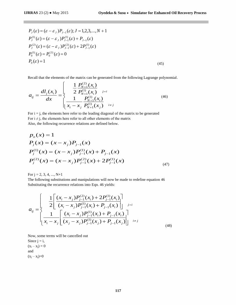
1)(
0)()(
)(2)()()(
)()()()(
1,...,3,2,1);()()(
0
)2(
0
)1(
0
)1(
1
)2(
1
)2(
1
)1(
1
)1(
1
P
PP
PPP
PPP
NJPP
JJJJ
JJJJ
JJJ
(45)
Recall that the elements of the matrix can be generated from the following Lagrange polynomial.
jijN
iN
ji
ijiN
iN
ij
ij
xP
xP
xx
xP
xP
dx
xdla
)(
)(1
)(
)(
2
1
)(
)1(
1
)1(
1
)1(
1
)2(
1
(46)
For i = j, the elements here refer to the leading diagonal of the matrix to be generated
For i ≠ j, the elements here refer to all other elements of the matrix
Also, the following recurrence relations are defined below.
)(2)()()(
)()()()(
)()()(
1)(
)1(
1
)2(
1
)2(
1
)1(
1
)1(
1
xPxPxxxP
xPxPxxxP
xPxxxP
xp
jjjj
jjjj
jjj
o
(47)
For j = 2, 3, 4, ..., N+1
The following substitutions and manipulations will now be made to redefine equation 46
Substituting the recurrence relations into Eqn. 46 yields:
jijjjjjj
ijijji
ji
ijijijji
ijijji
ij
xPxPxx
xPxPxx
xx
xPxPxx
xPxPxx
a
)()()(
)()()(1
)()()(
)(2)()(
2
1
1
)1(
1
1
)1(
1
1
)1(
1
)1(
1
)2(
1
(48)
Now, some terms will be cancelled out
Since j = i,
(xi – xj) = 0
and
(xj – xj)=0
IJRRAS 23 (2) ● May 2015 Oyedeko & Susu ● Simulator for Enhanced Oil Recovery Process
118
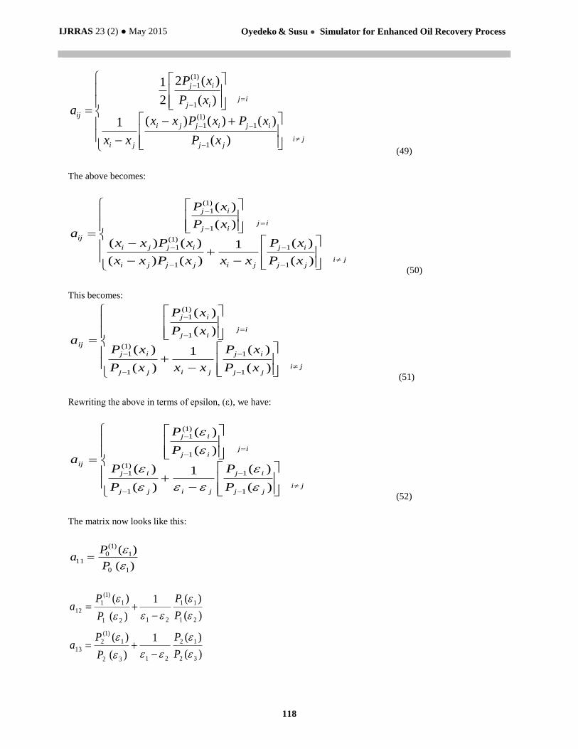
jijj
ijijji
ji
ijij
ij
ij
xP
xPxPxx
xx
xP
xP
a
)(
)()()(1
)(
)(2
2
1
1
1
)1(
1
1
)1(
1
(49)
The above becomes:
jijj
ij
jijjji
ijji
ijij
ij
ij
xP
xP
xxxPxx
xPxx
xP
xP
a
)(
)(1
)()(
)()(
)(
)(
1
1
1
)1(
1
1
)1(
1
(50)
This becomes:
jijj
ij
jijj
ij
ijij
ij
ij
xP
xP
xxxP
xP
xP
xP
a
)(
)(1
)(
)(
)(
)(
1
1
1
)1(1
1
)1(1
(51)
Rewriting the above in terms of epsilon, (ε), we have:
jijj
ij
jijj
ij
ijij
ij
ij
P
P
P
P
P
P
a
)(
)(1
)(
)(
)(
)(
1
1
1
)1(1
1
)1(1
(52)
The matrix now looks like this:
)(
)(
10
1
)1(
011
P
Pa
)(
)(1
)(
)(
21
11
2121
1
)1(
1
12
P
P
P
Pa
)(
)(1
)(
)(
32
12
2132
1
)1(
2
13
P
P
P
Pa
IJRRAS 23 (2) ● May 2015 Oyedeko & Susu ● Simulator for Enhanced Oil Recovery Process
119
)(
)(1
)(
)(
10
20
1210
2
)1(
0
21
P
P
P
Pa
)(
)(
11
2
)1(
1
22
P
Pa
)(
)(1
)(
)(
32
22
3232
2
)1(
2
23
P
P
P
Pa
)(
)(1
)(
)(
10
30
1310
3
)1(
0
31
P
P
P
Pa
)(
)(1
)(
)(
21
31
2321
3
)1(
1
32
P
P
P
Pa
)(
)(
32
3
)1(
2
32
P
Pa
(53)
The recurrence relations below will again be used to evaluate the terms of the matrix.
1
(1) (1)
1 1
(1)
0
( ) 1
( ) ( ) ( )
( ) ( ) ( ) ( )
( ) 0
o
j j j
j j j j
p
P P
P P P
P
(54)
Let ԑ assume the range
ԑ = [0:0.01:0.09]
where
ԑ1 = 0 (55)
ԑ2 = 0.01 (56)
ԑ3 = 0.02 (57)
3. RESULTS
The reservoir response, as predicted by the simulation on the basis of the theory of coherence, is compared with the
numerical predictions obtained using traditional finite difference method and orthogonal collocation. The case
studies are chosen to be both hypothetical and using of existing Nigerian well data with simple representative of the
important elements of the simulator. The main objective of these case studies has been to demonstrate that the
mathematical techniques of orthogonal collocation, finite difference and coherent theory in the context of
IJRRAS 23 (2) ● May 2015 Oyedeko & Susu ● Simulator for Enhanced Oil Recovery Process
120
application of the simulator can be used to obtain wave behaviour in a reservoir. A gradually increasing level of
complexity is introduced, representing a range of systems from aqueous phase flow, to surfactant chromatography in
two phase flow, to surfactant chromatography in two dimensional porous medium. The initial and injected surfactant
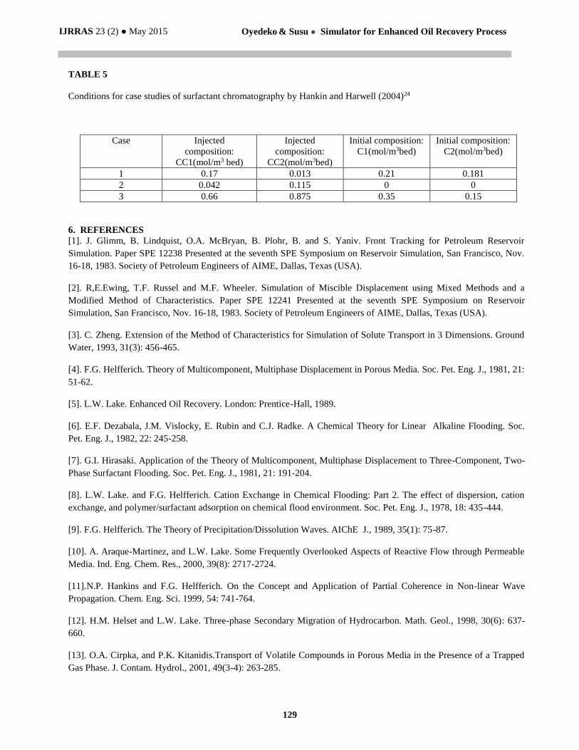
compositions corresponding to cases 1, 2 and 3 are shown in Table 5. The rock and fluid properties are listed in
Table 1, 2, 3, 4. These were taken as uniform for convenience.
The two fluid phases consisted of a water phase and an oil phase, which, for convenience are considered
incompressible. The density of oil, the viscosity of oil, the salinity of water, and the formation volume factor of oil
and water are listed in Table 2 in appendix. All cases mentioned above were run by using anionic sodium dodecyl
sulfate (SDS) and cationic dodecyl pyridinium chloride (DPC) as surfactants.
The system of equations is complete with the equations representing physical properties of the fluids and the rock.
The physical properties described here are: (1) phase behaviour (2) interfacial tension between fluid phases, (3)
residual phase saturations, (4) relative permeabilities, (5) rock wettabiliy, (6) phase viscosities, (7) capillary
pressure, (8) adsorption and (9) dispersion. From a physical-chemical point of view, there are three components -
water, petroleum and chemical. They are in fact, pseudo-components, since each one consists of several pure
components. Petroleum is a complex mixture of many hydrocarbons. Water is actually brine, and contains dissolved
salts. Finally, the chemical contains different kinds of surfactants.
These three pseudo-components are distributed between two phases –the oleic phase and the aqueous phase. The
chemical has an amphiphilic character. It makes the oleic phase at least partially miscible with water or the aqueous
phase at partially miscible with petroleum. Interfacial tension depends on the surfactant partition between the two
phases, and hence of phase behaviour. Residual phase saturation decreases as interfacial tension decreases. Relative
permeability parameters depend on residual phase saturations. Phase viscosities are functions of the volume fraction
of the components in each fluid phase. Therefore, the success or failure of surfactant flooding processes depends on
phase behaviour. Phase behaviour influences all other physical properties, and each of them, in turn influences oil
recovery.
For a two-phase flow of water and oil, where no surfactant partitions into the oleic phase, the same scenario is
obtained as the one dimensional injection for cases 1 and 2. The bed has an initial water saturation of 0.3, and is
flooded with an aqueous surfactant solution. The numerical profiles agree with the coherent wave profiles. The
effect of the two–phase flow is to elongate the waves, leading to a larger region of constant state and earlier
breakthrough of the fast wave.
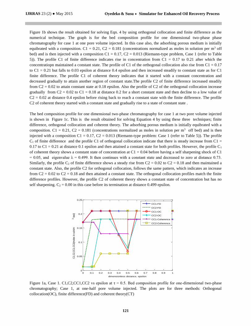
Figure 1a is the result obtained for solving Equation 4 using the three methods finite difference, orthogonal
collocation, coherent theory. The graph is for the composition profile for one dimensional two-phase
chromatography initially equilibrated with a composition C1 = 0.21, C2 = 0.181 and is then injected with a
composition C1 = 0.17, C2 = 0.013 (Riemann type problem, Case 1 (refer to Table 5)). In Figure 1a, the profile C1
of finite difference shows a steady rise from C1 = 0.17 to C1= 0.21 and then remain constant at this concentration.
The profile C1 of the orthogonal collocation increases steadily from C1 = 0.17 to C1 = 0.21 at distance 0.1 epsilon
maintaining a constant state to distance 0.3 epsilon. After this it started declining from C1 = 0.21 to C1 = 0.07 at
distance 0.5 epsilon before rising back to attain a constant state with the finite difference. The profile C1 of the
coherent theory on the other hand started with a constant state, then declined before continues with constant state
and rise again to attain constant state with the other profiles. Similarly, the profile C2 of finite difference increased
steadily from C2 = 0.017 to a constant state of C2 = 0.18 The orthogonal collocation for C2 starts at C2 = 0.01 for a
short constant state and then rise steadily to C2 = 0.18 to attain another short constant state from 0.2 to 0.3 epsilon.
From here it depressed to C2 = 0.07 before rising back to C2 = 0.18 and then attain a constant state with finite
difference. The profile C2 of coherent theory starts with a short constant state, then increases readily to C2 = 0.05
for another constant state from which it rises up to the final region of constant state with the other profiles.
IJRRAS 23 (2) ● May 2015 Oyedeko & Susu ● Simulator for Enhanced Oil Recovery Process
121
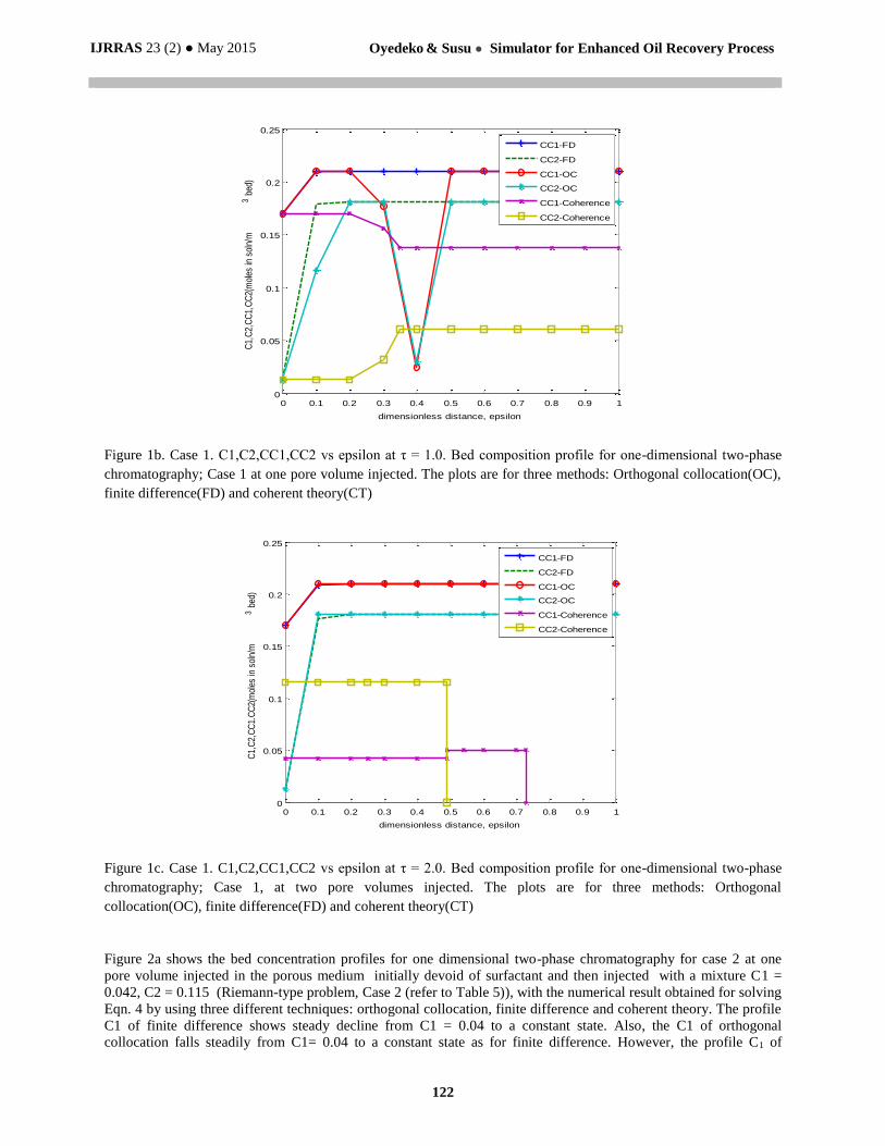
Figure 1b shows the result obtained for solving Eqn. 4 by using orthogonal collocation and finite difference as the
numerical technique. The graph is for the bed composition profile for one dimensional two-phase phase
chromatography for case 1 at one pore volume injected. In this case also, the adsorbing porous medium is initially
equibrated with a composition. C1 = 0.21, C2 = 0.181 (concentrations normalized as moles in solution per m3 off
bed) and is then injected with a composition C1 = 0.17, C2 = 0.013 (Riemann-type problem, Case 1 (refer to Table
5)). The profile C1 of finite difference indicates rise in concentration from C1 = 0.17 to 0.21 after which the
concentratiopn maintained a constant state. The profile of C1 of the orthogonal collocation also rise from C1 = 0.17
to C1 = 0.21 but falls to 0.03 epsilon at distance 0.4 epsilon and then increased steadily to constant state as for C1
finite difference. The profile C1 of coherent theory indicates that it started with a constant concentration and
decreased gradually to attain another region of constant state.The profile C2 of finite difference increased steadily
from C2 = 0.02 to attain constant state at 0.18 epsilon. Also the profile of C2 of the orthogonal collocation increase
gradually from C2 = 0.02 to C1 = 0.18 at distance 0.2 for a short constant state and then decline to a low value of
C2 = 0.02 at distance 0.4 epsilon before rising back to reach a constant state with the finite difference. The profile
C2 of coherent theory started with a constant state and gradually rise to a state of constant state .
The bed composition profile for one dimensional two-phase chromatography for case 1 at two pore volume injected
is shown in Figure 1c. This is the result obtained for solving Equation 4 by using these three techniques; finite
difference, orthogonal collocation and coherent theory. The adsorbing porous medium is initially equibrated with a
composition. C1 = 0.21, C2 = 0.181 (concentrations normalized as moles in solution per m3 off bed) and is then
injected with a composition C1 = 0.17, C2 = 0.013 (Riemann-type problem: Case 1 (refer to Table 5)). The profile
C1 of finite difference and the profile C1 of orthogonal collocation indicate that there is steady increase from C1 =
0.17 to C1 = 0.21 at distance 0.1 epsilon and then attained a constant state for both profiles. However, the profile C1
of coherent theory shows a constant state of concentration at C1 = 0.04 before having a self sharpening shock of C1
= 0.05, and eigenvalue λ = 0.499. It then continues with a constant state and decreased to zero at distance 0.73.
Similarly, the profile C2 of finite difference shows a steady rise from C2 = 0.02 to C2 = 0.18 and then maintained a
constant state. Also, the profile C2 for orthogonal collocation, follows the same pattern, which indicates an increase
from C2 = 0.02 to C2 = 0.18 and then attained a constant state. The orthogonal collocation profiles match the finite
difference profiles. However, the profile C2 of coherent theory shows a constant state of concentration but has no
self sharpening. C2 = 0.00 in this case before its termination at distance 0.499 epsilon.
Figure 1a, Case 1. C1,C2,CC1,CC2 vs epsilon at τ = 0.5. Bed composition profile for one-dimensional two-phase
chromatography; Case 1, at one-half pore volume injected. The plots are for three methods: Orthogonal
collocation(OC), finite difference(FD) and coherent theory(CT)
0 0.1 0.2 0.3 0.4 0.5 0.6 0.7 0.8 0.9 10
0.05
0.1
0.15
0.2
0.25
dimensionless distance, epsilon
C1,
C2,
CC
1,C
C2(
mol
es in
sol
n/m
3 b
ed)
CC1-FD
CC2-FD
CC1-OC
CC2-OC
CC1-Coherence
CC2-Coherence
IJRRAS 23 (2) ● May 2015 Oyedeko & Susu ● Simulator for Enhanced Oil Recovery Process
122
Figure 1b. Case 1. C1,C2,CC1,CC2 vs epsilon at τ = 1.0. Bed composition profile for one-dimensional two-phase
chromatography; Case 1 at one pore volume injected. The plots are for three methods: Orthogonal collocation(OC),
finite difference(FD) and coherent theory(CT)
Figure 1c. Case 1. C1,C2,CC1,CC2 vs epsilon at τ = 2.0. Bed composition profile for one-dimensional two-phase
chromatography; Case 1, at two pore volumes injected. The plots are for three methods: Orthogonal
collocation(OC), finite difference(FD) and coherent theory(CT)
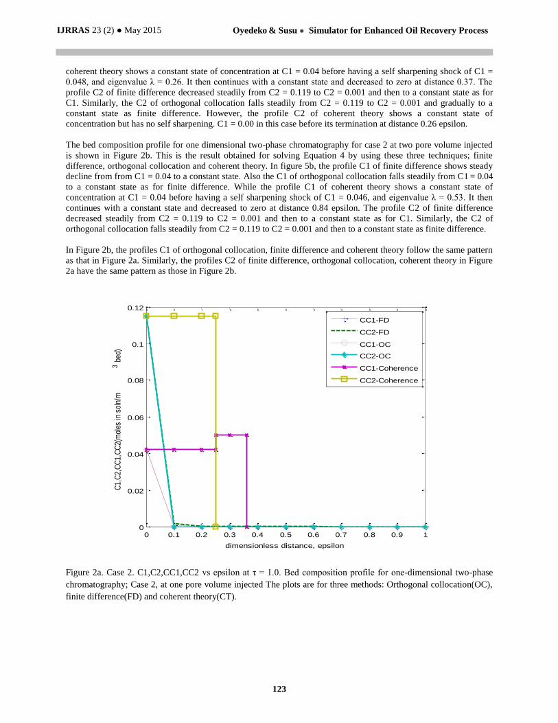
Figure 2a shows the bed concentration profiles for one dimensional two-phase chromatography for case 2 at one
pore volume injected in the porous medium initially devoid of surfactant and then injected with a mixture C1 =
0.042, C2 = 0.115 (Riemann-type problem, Case 2 (refer to Table 5)), with the numerical result obtained for solving
Eqn. 4 by using three different techniques: orthogonal collocation, finite difference and coherent theory. The profile
C1 of finite difference shows steady decline from C1 = 0.04 to a constant state. Also, the C1 of orthogonal
collocation falls steadily from C1= 0.04 to a constant state as for finite difference. However, the profile C1 of
0 0.1 0.2 0.3 0.4 0.5 0.6 0.7 0.8 0.9 10
0.05
0.1
0.15
0.2
0.25
dimensionless distance, epsilon
C1,
C2,
CC
1,C
C2(
mol
es in
sol
n/m
3 b
ed)
CC1-FD
CC2-FD
CC1-OC
CC2-OC
CC1-Coherence
CC2-Coherence
0 0.1 0.2 0.3 0.4 0.5 0.6 0.7 0.8 0.9 10
0.05
0.1
0.15
0.2
0.25
dimensionless distance, epsilon
C1,
C2,
CC
1.C
C2(
mol
es in
sol
n/m
3 b
ed)
CC1-FD
CC2-FD
CC1-OC
CC2-OC
CC1-Coherence
CC2-Coherence
IJRRAS 23 (2) ● May 2015 Oyedeko & Susu ● Simulator for Enhanced Oil Recovery Process
123
coherent theory shows a constant state of concentration at C1 = 0.04 before having a self sharpening shock of C1 =
0.048, and eigenvalue λ = 0.26. It then continues with a constant state and decreased to zero at distance 0.37. The
profile C2 of finite difference decreased steadily from C2 = 0.119 to C2 = 0.001 and then to a constant state as for
C1. Similarly, the C2 of orthogonal collocation falls steadily from C2 = 0.119 to C2 = 0.001 and gradually to a
constant state as finite difference. However, the profile C2 of coherent theory shows a constant state of
concentration but has no self sharpening. C1 = 0.00 in this case before its termination at distance 0.26 epsilon.
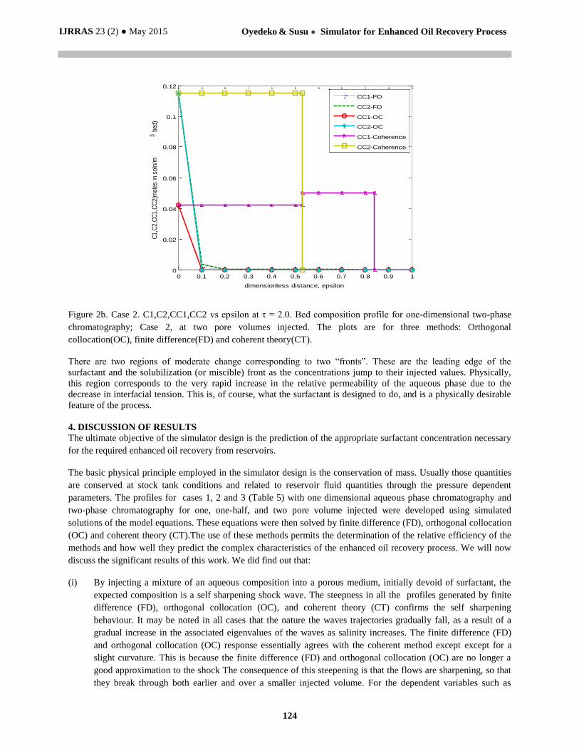
The bed composition profile for one dimensional two-phase chromatography for case 2 at two pore volume injected
is shown in Figure 2b. This is the result obtained for solving Equation 4 by using these three techniques; finite
difference, orthogonal collocation and coherent theory. In figure 5b, the profile C1 of finite difference shows steady
decline from from C1 = 0.04 to a constant state. Also the C1 of orthogponal collocation falls steadily from C1 = 0.04
to a constant state as for finite difference. While the profile C1 of coherent theory shows a constant state of
concentration at C1 = 0.04 before having a self sharpening shock of C1 = 0.046, and eigenvalue λ = 0.53. It then
continues with a constant state and decreased to zero at distance 0.84 epsilon. The profile C2 of finite difference
decreased steadily from C2 = 0.119 to C2 = 0.001 and then to a constant state as for C1. Similarly, the C2 of
orthogonal collocation falls steadily from C2 = 0.119 to C2 = 0.001 and then to a constant state as finite difference.
In Figure 2b, the profiles C1 of orthogonal collocation, finite difference and coherent theory follow the same pattern
as that in Figure 2a. Similarly, the profiles C2 of finite difference, orthogonal collocation, coherent theory in Figure
2a have the same pattern as those in Figure 2b.
Figure 2a. Case 2. C1,C2,CC1,CC2 vs epsilon at τ = 1.0. Bed composition profile for one-dimensional two-phase
chromatography; Case 2, at one pore volume injected The plots are for three methods: Orthogonal collocation(OC),
finite difference(FD) and coherent theory(CT).
0 0.1 0.2 0.3 0.4 0.5 0.6 0.7 0.8 0.9 10
0.02
0.04
0.06
0.08
0.1
0.12
dimensionless distance, epsilon
C1,
C2,
CC
1,C
C2(
mol
es in
sol
n/m
3 b
ed)
CC1-FD
CC2-FD
CC1-OC
CC2-OC
CC1-Coherence
CC2-Coherence
IJRRAS 23 (2) ● May 2015 Oyedeko & Susu ● Simulator for Enhanced Oil Recovery Process
124
Figure 2b. Case 2. C1,C2,CC1,CC2 vs epsilon at τ = 2.0. Bed composition profile for one-dimensional two-phase
chromatography; Case 2, at two pore volumes injected. The plots are for three methods: Orthogonal
collocation(OC), finite difference(FD) and coherent theory(CT).
There are two regions of moderate change corresponding to two “fronts”. These are the leading edge of the
surfactant and the solubilization (or miscible) front as the concentrations jump to their injected values. Physically,
this region corresponds to the very rapid increase in the relative permeability of the aqueous phase due to the
decrease in interfacial tension. This is, of course, what the surfactant is designed to do, and is a physically desirable
feature of the process.
4. DISCUSSION OF RESULTS
The ultimate objective of the simulator design is the prediction of the appropriate surfactant concentration necessary
for the required enhanced oil recovery from reservoirs.
The basic physical principle employed in the simulator design is the conservation of mass. Usually those quantities
are conserved at stock tank conditions and related to reservoir fluid quantities through the pressure dependent
parameters. The profiles for cases 1, 2 and 3 (Table 5) with one dimensional aqueous phase chromatography and
two-phase chromatography for one, one-half, and two pore volume injected were developed using simulated
solutions of the model equations. These equations were then solved by finite difference (FD), orthogonal collocation
(OC) and coherent theory (CT).The use of these methods permits the determination of the relative efficiency of the
methods and how well they predict the complex characteristics of the enhanced oil recovery process. We will now
discuss the significant results of this work. We did find out that:
(i) By injecting a mixture of an aqueous composition into a porous medium, initially devoid of surfactant, the
expected composition is a self sharpening shock wave. The steepness in all the profiles generated by finite
difference (FD), orthogonal collocation (OC), and coherent theory (CT) confirms the self sharpening
behaviour. It may be noted in all cases that the nature the waves trajectories gradually fall, as a result of a
gradual increase in the associated eigenvalues of the waves as salinity increases. The finite difference (FD)
and orthogonal collocation (OC) response essentially agrees with the coherent method except except for a
slight curvature. This is because the finite difference (FD) and orthogonal collocation (OC) are no longer a
good approximation to the shock The consequence of this steepening is that the flows are sharpening, so that
they break through both earlier and over a smaller injected volume. For the dependent variables such as
0 0.1 0.2 0.3 0.4 0.5 0.6 0.7 0.8 0.9 10
0.02
0.04
0.06
0.08
0.1
0.12
dimensionless distance, epsilon
C1,
C2,
CC
1,C
C2(
mol
es in
sol
n/m
3 b
ed)
CC1-FD
CC2-FD
CC1-OC
CC2-OC
CC1-Coherence
CC2-Coherence
IJRRAS 23 (2) ● May 2015 Oyedeko & Susu ● Simulator for Enhanced Oil Recovery Process
125
component concentration, common velocity exists at each point in the wave, and the associated composition
route and relative shifts of waves associated with other dependent variable waves remains unchanged. This
was confirmed for all numerical methods, in agreement with the work of Helferich4.
(ii) By injecting a mixture of low concentration aqueous surfactant composition into adsorbing porous medium
that is initially injected with high concentration of aqueous surfactant composition, a variation may exist in
the initial profile or a new profile may be generated by the injection. The initial fluid or previously injected
fluid has the same composition downstream of the change while the newly injected fluid has the same
composition upstream of the original variation. The composition route along the bed follows the slow path
from the injected composition and then switches to the fast path leading to the previously injected
compòsition. The route passes along the paths in the sequence of increasing wave velocities.
(iii) By injecting a mixture of high concentration of surfactant into adsorbing porous medium that is initially
injected with low concentration of aqueous surfactant composition, we encountered two types of path: the
slow and fast paths. The slow path eigenvalues are closer to the fast path eigenvalues with values of 1; the
effect of dispersion results in the merging of the two waves. This is due to their spatial position, and loss of
intermediate region of constant state. However, this region later reappears as dispersion decreases.
(iv) For a system of two phase (aqueous and oleic) flow of water and oil in which there is no surfactant partitions
into the oleic phase, the effect of two phase flow is the elongation of the wave, leading to a larger region of
constant state and earlier breakthrough of fast wave. The shock and wave composition routes are identical to
that of the aqueous phase and has a unique composition path grid which is independent of the saturation of
the flowing phases. This is similar to system of two-phase (aqueous and oleic) flow in which two water
soluble components partition between an aqueous and a solid adsorbent with the use of low concentration
surfactants to improve volumetric sweep efficiency during surfactant assisted waterflooding in certain
enhanced oil recovery techniques19.
(v) When surfactant partitions into the oleic phase, the effect is that the adsorption of the surfactant in the solid
phase results in the formation of micelles which then break away from the solid phase and move much faster
than the surfactant in the oleic phase. The domination of the micelle formation in the aqueous phase is the
general effect for both slow and fast phases. The presence of the two partitioning components does not alter
the fractional flow relations fj(Sj) for the two phases.The sum of the aqueous and oleic phase saturations must
add up to one wave of the saturation variables.
(vi) The comparison between the coherent theory (CT) and finite difference (FD) and orthogonal collocation (OC)
simulated results are not based on closed solutions of the transport equations, but on inexact solutions of these
equations. This is in spite of the fact that the methods are based on the conservation of mass, containing the
same physical properties. The slight differences are due to assumed discrete values used base on the method.
The coherent wave fronts match the wave fronts for finite difference and orthogonal collocation at their points
of turning, where the effective wave dispersion is zero.
The simulation results of the predicted profiles by the coherent theory (CT), finite difference (FD) and orthogonal
collocation (OC) techniques illustrate the typical effects of a pattern flood such as the early breakthrough of
the oil bank and the long tail on the oil surfactant curves. The results show only significant deviations in some
sections. The only significant difference beween the coherent theory (CT) and finite difference (FD) results is
that the finite difference (FD) profiles are continous while the coherent profiles are discontinous. More
oscillations are evident in the orthogonal collocation (OC) solution profiles. This indicates that orthogonal
collocation (OC) solution is sensitive to oscillation than other methods. This is particularly noticeable in the
curves following breakthrough. The finite difference (FD) is considerably more dissipative and therefore the
small oscillations are absent. Also the coherent suppresses oscillation and is less dissipative. These findings
IJRRAS 23 (2) ● May 2015 Oyedeko & Susu ● Simulator for Enhanced Oil Recovery Process
126
are beyond the findings of Hankins and Harwell19. For the findings of Hankins and Harwell19 did not show
and explain these salient findings.
(vii) Several simulations were made to evaluate the dependence of oil recovery on slug size for a given amount of
injected surfactant. This is an important design factor. It is generally thought that a large dilute slug will be
better in a heterogeneous reservoir. This seems intuitively correct since a small slug would seem to be
proportioned into the lowest permeabilities in such a small amount that little, if any, oil recovery from those
parts of the reservoir could be expected. This by itself, would not be an unreasonable strategy. The
dependence of oil recovery on slug size for a given amount of injected surfactant or for a fixed product of
slug size and surfactant concentration indicates that the more surfactant injected, the more oil is recovered.
This is because an injected surfactant disperses into oil and water, then lower the interfacial tension thereby
mobilized more immobile oil. This is continued until the surfactant is diluted or lost due to adsorption by the
rock. For significant incremental oil recoveries, several orders of magnitude reduction is needed. Hence, large
quantities of surfactant are required for reduction of the interfacial tension to produce the desired effect. So,
the effect of surfactant slug size is predictable.Also, the effect of surfactant concentration is also predictable
in the same manner as more oil is recovered for increase in surfactant concentration injected.
Some of the complexities outlined above could not have been predicted by using only the coherent technique by
Hankins and Harwell24. This is a major accomplishment of this work. Not only was the discontinuities predicted by
this work, it also provides an insight into the complex behaviour of enhanced oil recovery process.
5. CONCLUSIONS
The applicability of solutions of the model transport equations for the design of the simulator in a multiphase,
multicomponent flow and transport in a reservoir has been demonstrated using orthogonal collocation solution. The
results of the orthogonal collocation solution were compared with those of finite difference and coherence solutions.
The results obtained using this methodology revealed certain features unobserved by the published work of Hankins
and Harwell26. The results indicate that the concentration of surfactants (C1, C2) for orthogonal collocation appear to
show more features than the predictions of the coherence and finite difference solutions. The reason for the
difference is the subject of continuing study by our team. It is unlikely that the coherence approach could ultimately
accommodate the complexities required for a thorough understanding of the full field reservoir simulator.
It is obvious that the coherent routes for the compositions of adsorbing surfactants correspond to the simpler case of
aqueous phase chromatography, with modified eigenvalue. This observation also holds for “shock” waves. The
existence of a partially coherent solution makes the prediction of reservoir response much more straightforward.
However, the ‘partially’ coherent solution only exist if surfactants does not partition into the oleic phase and
fractional flow is not a function of surfactant composition; should either occur, a globally coherent solution may still
be found, but the solution is more complex and difficult to handle. There is no equivalence of partial coherence in
the orthogonal and finite difference methods. Therein lies the possibility of the differences in the concentration
profiles predicted by the three numerical techniques. Again, the use of the orthogonal collocation and finite
difference solution provides easier solution to future possible problems that may arise as the simulator is being
used.
The dependence of oil recovery on slug size for a given amount of injected surfactant indicates that the more
surfactant injected the more oil is recovered. For significant incremental oil recoveries, several order of magnitude
interfacial tension reduction is needed. Hence, large quantities of surfactant are required to produce the desired
effect of high oil recovery.
IJRRAS 23 (2) ● May 2015 Oyedeko & Susu ● Simulator for Enhanced Oil Recovery Process
127
TABLE 1
Reservoir characteristics from the work of Hankins and Harwell24
Parameter Value
Rock density 2.65 g/cm3
Porosity 0.2
Oil viscosity 5.0 cp
Water viscosity 1.0 cp
Injection pressure gradient
( maintained constant )
1.5 psi/ft
Fluid densities 1.0 g/cm3
Width of injection face 50 ft
Width of central high permeability streak 10 ft
Length of reservoir 100 or 5000 ft
Residual oil saturation 0.2
Connate water saturation 0.1
First injected surfactant SDS
Second injected surfactant DPC
Henry’s law constant
SDS
DPC
2.71×10⁻⁴ l/g
8.30×10⁻⁵ l/g
CMC Values
SDS
DPC
800 μmol/l
4000 μmoll/l
Injected concentration
SDS
DPC
10 CMC
10 CMC
Brine spacer (typical) ≈ 0.05 pore volumes
Slug volumes ≈ 0.10 pore volumes
TABLE 2
Reservoir Characteristics used for the Simulation work by Oyedeko 25
Parameter Value
Rock density 2.65 g/cm3
Porosity 0.2
Oil viscosity 0.40 cp
Water viscosity 0.30 cp
Injection pressure gradient
( maintained constant )
1.5 psi/ft
Fluid densities 1.0 g/cm3
Width of injection face 50 ft
Width of central high permeability streak 10 ft
Length of reservoir 100 or 5000 ft
Residual oil saturation 0.2
Connate water saturation 0.2
First injected surfactant SDS
Second injected surfactant DPC
Henry’s law constant
SDS
DPC
2.71×10⁻⁴ l/g
8.30×10⁻⁵ l/g
CMC Values
SDS
DPC
800 μmol/l
4000 μmoll/l
Injected concentration
SDS
DPC
10 CMC
10 CMC
Brine spacer (typical) ≈ 0.05 pore volumes
Slug volumes ≈ 0.10 pore volumes
IJRRAS 23 (2) ● May 2015 Oyedeko & Susu ● Simulator for Enhanced Oil Recovery Process
128
TABLE 3
Parameter values used in Trogus adsorption model for verification runs26
Parameter Value
Pure component CMCs C1*=1.0 mol/m3
C2*=0.35 mol/m3
Phase separation model parameter θ=1.8
Henry’s law constants for adsorption
,i i i wC k C
(,i wC = aqueous monomer concentration)
k1 =0.21×10⁻³ m3/kg
k2= 0.80×10⁻³ m3/kg
Henry’s law constant for oleic partitioning , ,i o i i wC q C
(,i wC = aqueous monomer concentration)
q1=7.1
q2=1.3
Adsorbent properties ρs =2.1× 10+3 m3/kg
∅ =0.2
TABLE 4
Additional Reservoir Parameters for the coherence work by Hankin and Harwell (2004)24
Model designation A B
Grid points in the horizontal direction ( m+1) 21 21
Grid points in the vertical direction (n+1) 11 21
Coherent waves of water saturation 28 28
Initial number of points per coherent wave
Water
Surfactant
41
81
41
81
Maximum number of points required per coherent wave ≈ 300 ≈300
Average time step size (days)
Short reservoir (100 ft)
200 mD streak
1000 mD streak
Long reservoir (5000ft)
200 mD streak
1000 mD sreak
3.47
0.69
174.0
34.7
3.47
0.69
174.0
34.7
Typical number of time steps required to inject first pore
volume
Short reservoir
Long reservoir
33
75
33
75
IJRRAS 23 (2) ● May 2015 Oyedeko & Susu ● Simulator for Enhanced Oil Recovery Process
129
TABLE 5
Conditions for case studies of surfactant chromatography by Hankin and Harwell (2004)24
Case Injected
composition:
CC1(mol/m3 bed)
Injected
composition:
CC2(mol/m3bed)
Initial composition:
C1(mol/m3bed)
Initial composition:
C2(mol/m3bed)
1 0.17 0.013 0.21 0.181
2 0.042 0.115 0 0
3 0.66 0.875 0.35 0.15
6. REFERENCES
[1]. J. Glimm, B. Lindquist, O.A. McBryan, B. Plohr, B. and S. Yaniv. Front Tracking for Petroleum Reservoir
Simulation. Paper SPE 12238 Presented at the seventh SPE Symposium on Reservoir Simulation, San Francisco, Nov.
16-18, 1983. Society of Petroleum Engineers of AIME, Dallas, Texas (USA).
[2]. R,E.Ewing, T.F. Russel and M.F. Wheeler. Simulation of Miscible Displacement using Mixed Methods and a
Modified Method of Characteristics. Paper SPE 12241 Presented at the seventh SPE Symposium on Reservoir
Simulation, San Francisco, Nov. 16-18, 1983. Society of Petroleum Engineers of AIME, Dallas, Texas (USA).
[3]. C. Zheng. Extension of the Method of Characteristics for Simulation of Solute Transport in 3 Dimensions. Ground
Water, 1993, 31(3): 456-465.
[4]. F.G. Helfferich. Theory of Multicomponent, Multiphase Displacement in Porous Media. Soc. Pet. Eng. J., 1981, 21:
51-62.
[5]. L.W. Lake. Enhanced Oil Recovery. London: Prentice-Hall, 1989.
[6]. E.F. Dezabala, J.M. Vislocky, E. Rubin and C.J. Radke. A Chemical Theory for Linear Alkaline Flooding. Soc.
Pet. Eng. J., 1982, 22: 245-258.
[7]. G.I. Hirasaki. Application of the Theory of Multicomponent, Multiphase Displacement to Three-Component, Two-
Phase Surfactant Flooding. Soc. Pet. Eng. J., 1981, 21: 191-204.
[8]. L.W. Lake. and F.G. Helfferich. Cation Exchange in Chemical Flooding: Part 2. The effect of dispersion, cation
exchange, and polymer/surfactant adsorption on chemical flood environment. Soc. Pet. Eng. J., 1978, 18: 435-444.
[9]. F.G. Helfferich. The Theory of Precipitation/Dissolution Waves. AIChE J., 1989, 35(1): 75-87.
[10]. A. Araque-Martinez, and L.W. Lake. Some Frequently Overlooked Aspects of Reactive Flow through Permeable
Media. Ind. Eng. Chem. Res., 2000, 39(8): 2717-2724.
[11].N.P. Hankins and F.G. Helfferich. On the Concept and Application of Partial Coherence in Non-linear Wave
Propagation. Chem. Eng. Sci. 1999, 54: 741-764.
[12]. H.M. Helset and L.W. Lake. Three-phase Secondary Migration of Hydrocarbon. Math. Geol., 1998, 30(6): 637-
660.
[13]. O.A. Cirpka, and P.K. Kitanidis.Transport of Volatile Compounds in Porous Media in the Presence of a Trapped
Gas Phase. J. Contam. Hydrol., 2001, 49(3-4): 263-285.
IJRRAS 23 (2) ● May 2015 Oyedeko & Susu ● Simulator for Enhanced Oil Recovery Process
130
[14]. J.R. Patton, K.H. Coats and G.T. Colegrove. Prediction of Polymer Flood Performance. Soc.Pet. Eng., 1971, 11:
72-84.
[15]. F.J. Fayers and R.I. Perrine. Mathematical Description of Detergent Flooding in Oil Reservoirs. Petroleum Trans.
AIME, 1959, 216: 277-283.
[16]. E.L. Claridge and P.I. Bondor. (1974). A Graphical Method for Calculating Linear Displacement with Mass
Transfer and Continuously Changing Mobilities. Soc. Pet. Eng. J., 1974, 14; 609-618.
[17]. R.G. Larson. The Influence of Phase Behaviour on Surfactant Flooding. Soc. Pet. Eng. J., 1979, 19: 411-422.
[18]. G.A. Pope, G.F. Carey and K. Sepehrnoori. Isothermal, Multiphase, Multicomponent Fluid Flow in Permeable
Media. Part II: Numerical Techniques and Solution. In Situ, 1984, 8(1): 1-40
[19] N.P. Hankins and J.H. Harwell. Case Studies for the Feasibility of Sweep Improvement in Surfactant-assisted
Waterflooding. J. Pet. Sci. Eng., 1997, 17: 41-62.
[20]. L. Siggel, M. Santa, M. Hansch, M. Nowak, M. Ranft, H. Weiss, D. Hajnal, E. Schreiner, G. Oetter, G. and J.
Tinsley. A New Class of Viscoelastic Surfactants for Enhanced Oil Recovery BASFSE SPE Improved Oil Recovery
Symposium, 14-18 April, 2001, Tulsa, Oklahoma, USA
[21]. Y. Xu, and M. Lu. Microbially Enhanced Oil Recovery at Simulated Reservoir Conditions by Use of
Engineered Bacteria. J. Petr. Sci. Eng., 2001, 78(2): 233-238.
[22]. A. Leach, A. and C.F. Mason. Co-optimization of Enhanced Oil Recovery and Carbon Sequestration. J.
Resource and Energy Economics. Resourse Energy Econ., 2011, 33(4): 893-912.
[23]. J.H. Harwell. Enhanced Oil Recovery Made Simple. J. Petr. Technol., 2012, 60(10): 42-43.
[24] N.P. Hankins. and J.H. Harwell. Application of Coherence Theory to a Reservoir Enhanced Oil Recovery
Simulator. J. Pet. Sci. Eng., 2004, 42: 29-55.
[25]. K.F. Oyedeko. Design and Development of a Simulator for a Reservoir Enhanced Oil Recovery Process. PhD
Dissertation, Lagos State University, Ojo, Lagos, Nigeria, 2014.
[26]. F.J. Trogus, R.S. Schecchter, G.A. Pope and W.H. Wade. New Interpretation of Adsorption Maxima and
Minima. J. Colloid Interface Sci., 1979, 70(3): 293-305.
[27]. F.G. Helfferich. Multicomponent Wave Propagation: Attainment of coherence from arbitrary starting
conditions. Chem. Eng. Comm., 1986, 44: 275-285.
[28] J.V. Villadsen and W.E. Stewart. Solution of Boundary Value Problems by Orthogonal Collocation. Chem.
Eng. Sci., 1967, 22: 1483-1501.
[29] J.V. Villadsen and W.E. Stewart. Solution of Boundary Value Problems by Orthogonal Collocation. Chem.
Eng. Sci., 1968, 23: 1515.