Applied Energy 115 (2014) 242–253

Contents lists available at ScienceDirect

Applied Energy

journal homepage: www.elsevier .com/ locate/apenergy

Comparison of different lead–acid battery lifetime prediction modelsfor use in simulation of stand-alone photovoltaic systems

0306-2619/$ - see front matter � 2013 Elsevier Ltd. All rights reserved.http://dx.doi.org/10.1016/j.apenergy.2013.11.021

⇑ Corresponding author. Tel.: +34 876555124; fax: +34 976762226.E-mail address: rdufo@unizar.es (R. Dufo-López).

Rodolfo Dufo-López ⇑, Juan M. Lujano-Rojas, José L. Bernal-AgustínElectrical Engineering Department. University of Zaragoza, C/María de Luna, 3, 50018 Zaragoza, Spain

h i g h l i g h t s

� Lifetime estimation of lead–acid batteries is a complex task.� This paper compares different models to predict battery lifetime in stand-alone systems.� We compare a weighted Ah-throughput battery ageing model with other models.� The battery charge controller significantly affects the lifetime of batteries.� The results show the weighted Ah-throughput model provides more accurate values.

a r t i c l e i n f o

Article history:Received 4 July 2013Received in revised form 31 October 2013Accepted 6 November 2013Available online 30 November 2013

Keywords:Lead–acid batteryPhotovoltaicStand-alone systemsLifetimeDegradationCorrosion

a b s t r a c t

Lifetime estimation of lead–acid batteries in stand-alone photovoltaic (PV) systems is a complex taskbecause it depends on the operating conditions of the batteries. In many research simulations and opti-misations, the estimation of battery lifetime is error-prone, thus producing values that differ substan-tially from the real ones. This error can indicate that the ‘‘optimal’’ system selected by theoptimisation tool will not be optimal. In this paper, all of the components of a PV system have been con-sidered simultaneously to simulate the behaviour of the system. One of these important components isthe battery charge controller, which significantly affects the lifetime of batteries. The results of the sim-ulations have allowed a comparison of the most common methods of battery lifetime prediction used bysimulation and/or optimisation tools with a weighted Ah-throughput method developed a few years ago.The results show that this recent method provides more accurate lifetime values. In a simulation of a realoff-grid household PV system where the real battery lifetime was 6.2 years, the weighted Ah-throughputmodel predicted a lifetime of 5.8 years; however, the other methods obtained lifetimes of more than15 years. In a simulation of another PV system designed to supply the load of an alarm where the realbatteries lifetime was 5.1 years, the weighted Ah-throughput model predicted a lifetime of 4.4 years;however, the other methods obtained lifetimes of more than nine years.

� 2013 Elsevier Ltd. All rights reserved.

1. Introduction

The ageing mechanisms of lead–acid batteries have been stud-ied previously [1–5]. The most important ageing processes are ano-dic corrosion, positive active mass degradation and the loss ofadherence to the grid, irreversible formation of lead sulphate inthe active mass, short-circuit, loss of water and electrolyte stratifi-cation [3]. These processes are often inter-dependent.

Batteries subject to deep cycling regimes typically age by degra-dation of the structure of the positive active mass. The battery cy-cle lifetime shown in the datasheet of the batteries (usually300–2000 full cycles depending on the technology) is obtained inlaboratory tests under standard conditions. However, the real

conditions of the cycles in PV systems are habitually very differentfrom standard conditions and the real cycle lifetime can be muchlower.

Stationary batteries, which operate under float-charge condi-tions (in practice, float service may also include occasional partialdischarges), typically age by corrosion of the positive grid. Underoptimum float voltage conditions (i.e., without cycling), a theoret-ical maximum service life can be achieved, called floating lifetime.Its value is between 10 and 20 years depending on the technology(manufacturers usually show this value in datasheets). However,even in the batteries of UPS systems (operating at float service)the real conditions can be different from optimal, and the realfloating life can be much lower than shown in the datasheet. Floatlife shown in the datasheet is usually reported at 20 or 25 �C, butthe effect of temperature on float life is approximately a 50% reduc-tion for every 8.3 �C increase in temperature [6].

R. Dufo-López et al. / Applied Energy 115 (2014) 242–253 243

Battery lifetime prediction in stand-alone systems is a difficulttask as it highly depends on the operating conditions. Many factorsaffect the life of the batteries, including the depth of the charge–discharge cycles, the current, the cell voltage, the performance ofthe charge controller (e.g., voltage and state of charge limits andregulation), the length of time that the batteries are in a low stateof charge, the time since the last full charge, the temperature, etc.

Many studies have been published about the simulation andoptimisation of renewable stand-alone systems including batter-ies. However, the battery lifetime has always been estimated infixed values based on the experience of the researcher [7–16] orit has been estimated by calculating the number of equivalent fullcycles [17–20]. In the best cases, it may be estimated using the cy-cle counting method [21–25]. Additionally, many simulation andoptimisation software tools use these methodologies to estimatebattery lifetimes [26–29]. However, the real lifetime of the batter-ies can differ from the estimated lifetime by many years using thementioned methods, depending on the operating conditions. Ahigh error in the estimation of the battery lifetime would imply agreat error in the estimation of the total cost of the batteries inthe net present cost (NPC) of the system; therefore, a real levelisedcost of energy (LCE) may be very different from the expectation.This fact can imply that, when using optimisation tools, the se-lected design for the system can be very far from the optimal one.

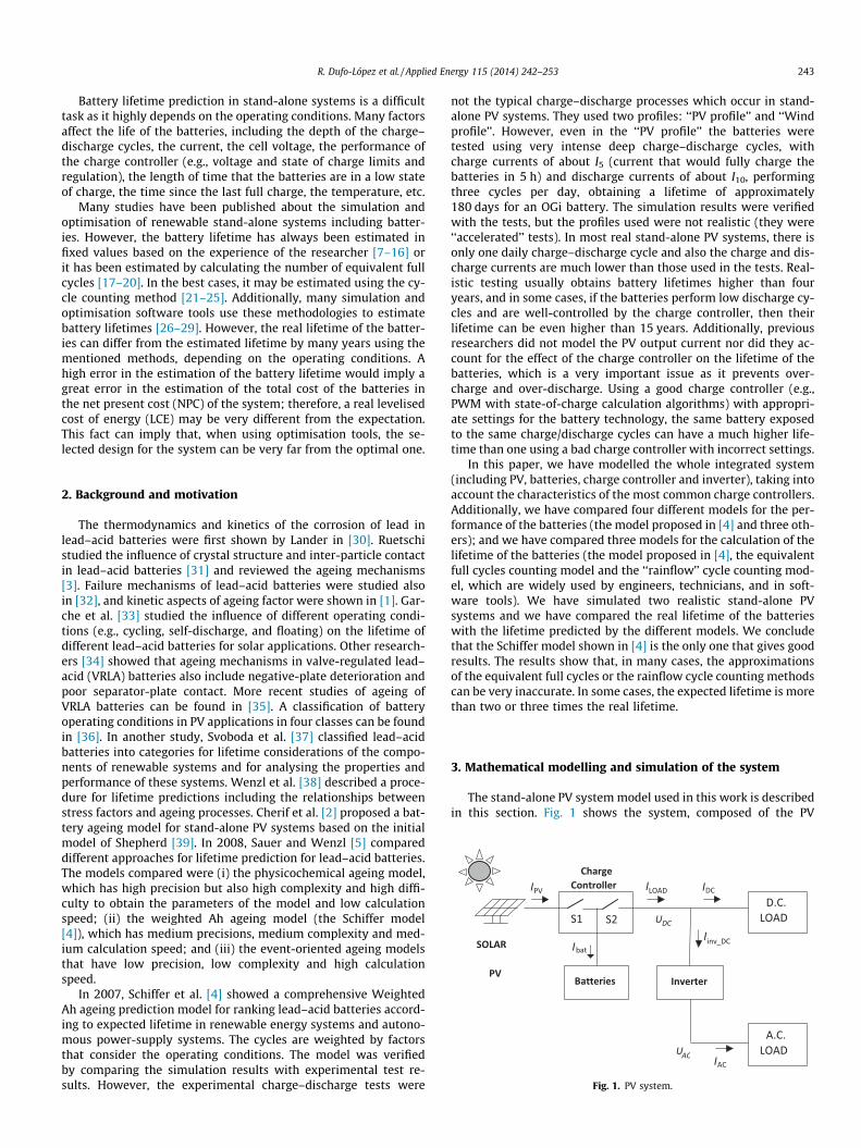
Fig. 1. PV system.

2. Background and motivation

The thermodynamics and kinetics of the corrosion of lead inlead–acid batteries were first shown by Lander in [30]. Ruetschistudied the influence of crystal structure and inter-particle contactin lead–acid batteries [31] and reviewed the ageing mechanisms[3]. Failure mechanisms of lead–acid batteries were studied alsoin [32], and kinetic aspects of ageing factor were shown in [1]. Gar-che et al. [33] studied the influence of different operating condi-tions (e.g., cycling, self-discharge, and floating) on the lifetime ofdifferent lead–acid batteries for solar applications. Other research-ers [34] showed that ageing mechanisms in valve-regulated lead–acid (VRLA) batteries also include negative-plate deterioration andpoor separator-plate contact. More recent studies of ageing ofVRLA batteries can be found in [35]. A classification of batteryoperating conditions in PV applications in four classes can be foundin [36]. In another study, Svoboda et al. [37] classified lead–acidbatteries into categories for lifetime considerations of the compo-nents of renewable systems and for analysing the properties andperformance of these systems. Wenzl et al. [38] described a proce-dure for lifetime predictions including the relationships betweenstress factors and ageing processes. Cherif et al. [2] proposed a bat-tery ageing model for stand-alone PV systems based on the initialmodel of Shepherd [39]. In 2008, Sauer and Wenzl [5] compareddifferent approaches for lifetime prediction for lead–acid batteries.The models compared were (i) the physicochemical ageing model,which has high precision but also high complexity and high diffi-culty to obtain the parameters of the model and low calculationspeed; (ii) the weighted Ah ageing model (the Schiffer model[4]), which has medium precisions, medium complexity and med-ium calculation speed; and (iii) the event-oriented ageing modelsthat have low precision, low complexity and high calculationspeed.

In 2007, Schiffer et al. [4] showed a comprehensive WeightedAh ageing prediction model for ranking lead–acid batteries accord-ing to expected lifetime in renewable energy systems and autono-mous power-supply systems. The cycles are weighted by factorsthat consider the operating conditions. The model was verifiedby comparing the simulation results with experimental test re-sults. However, the experimental charge–discharge tests were

not the typical charge–discharge processes which occur in stand-alone PV systems. They used two profiles: ‘‘PV profile’’ and ‘‘Windprofile’’. However, even in the ‘‘PV profile’’ the batteries weretested using very intense deep charge–discharge cycles, withcharge currents of about I5 (current that would fully charge thebatteries in 5 h) and discharge currents of about I10, performingthree cycles per day, obtaining a lifetime of approximately180 days for an OGi battery. The simulation results were verifiedwith the tests, but the profiles used were not realistic (they were‘‘accelerated’’ tests). In most real stand-alone PV systems, there isonly one daily charge–discharge cycle and also the charge and dis-charge currents are much lower than those used in the tests. Real-istic testing usually obtains battery lifetimes higher than fouryears, and in some cases, if the batteries perform low discharge cy-cles and are well-controlled by the charge controller, then theirlifetime can be even higher than 15 years. Additionally, previousresearchers did not model the PV output current nor did they ac-count for the effect of the charge controller on the lifetime of thebatteries, which is a very important issue as it prevents over-charge and over-discharge. Using a good charge controller (e.g.,PWM with state-of-charge calculation algorithms) with appropri-ate settings for the battery technology, the same battery exposedto the same charge/discharge cycles can have a much higher life-time than one using a bad charge controller with incorrect settings.

In this paper, we have modelled the whole integrated system(including PV, batteries, charge controller and inverter), taking intoaccount the characteristics of the most common charge controllers.Additionally, we have compared four different models for the per-formance of the batteries (the model proposed in [4] and three oth-ers); and we have compared three models for the calculation of thelifetime of the batteries (the model proposed in [4], the equivalentfull cycles counting model and the ‘‘rainflow’’ cycle counting mod-el, which are widely used by engineers, technicians, and in soft-ware tools). We have simulated two realistic stand-alone PVsystems and we have compared the real lifetime of the batterieswith the lifetime predicted by the different models. We concludethat the Schiffer model shown in [4] is the only one that gives goodresults. The results show that, in many cases, the approximationsof the equivalent full cycles or the rainflow cycle counting methodscan be very inaccurate. In some cases, the expected lifetime is morethan two or three times the real lifetime.

3. Mathematical modelling and simulation of the system

The stand-alone PV system model used in this work is describedin this section. Fig. 1 shows the system, composed of the PV

244 R. Dufo-López et al. / Applied Energy 115 (2014) 242–253

generator, charge controller, batteries and inverter. The load can beDC and/or AC.

3.1. PV generator

Calculating the hourly electricity generation of the PV generatorrequires knowledge of the hourly incident radiation in a typicalyear. In the cases where there is no irradiation hourly data avail-able, we have used the average daily radiation on a horizontal sur-face for each month of the year as the solar input data. The data areconverted into the average clearness index for each month usingthe Rietveld equation [40]. Then, the clearness index is obtainedfor each day of the year and the global hourly irradiation overthe surface of the PV panels is calculated according to the Grahammodel [41]. The Graham method is suitable because it takes intoaccount the uncertainty associated with the available irradiationdata.

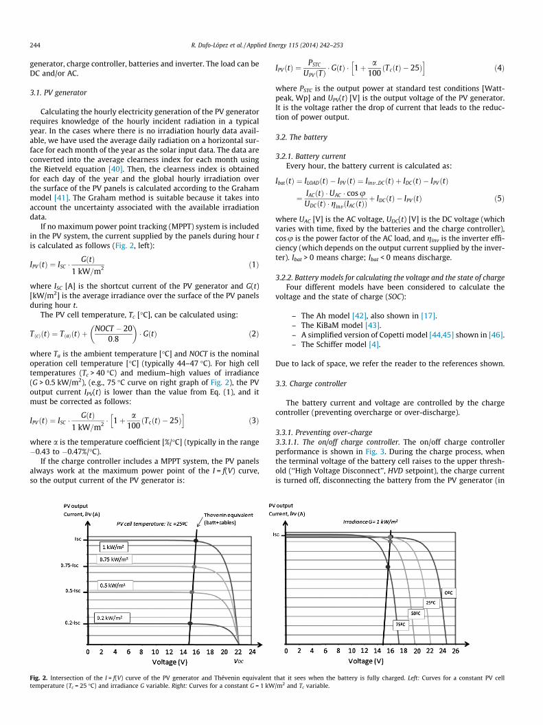
If no maximum power point tracking (MPPT) system is includedin the PV system, the current supplied by the panels during hour tis calculated as follows (Fig. 2, left):

IPV ðtÞ ¼ ISC �GðtÞ

1 kW=m2 ð1Þ

where ISC [A] is the shortcut current of the PV generator and G(t)[kW/m2] is the average irradiance over the surface of the PV panelsduring hour t.

The PV cell temperature, Tc [�C], can be calculated using:

TðcÞðtÞ ¼ TðaÞðtÞ þNOCT � 20

0:8

� �� GðtÞ ð2Þ

where Ta is the ambient temperature [�C] and NOCT is the nominaloperation cell temperature [�C] (typically 44–47 �C). For high celltemperatures (Tc > 40 �C) and medium–high values of irradiance(G > 0.5 kW/m2), (e.g., 75 �C curve on right graph of Fig. 2), the PVoutput current IPV(t) is lower than the value from Eq. (1), and itmust be corrected as follows:

IPV ðtÞ ¼ ISC �GðtÞ

1 kW=m2 � 1þ a100ðTcðtÞ � 25Þ

h ið3Þ

where a is the temperature coefficient [%/�C] (typically in the range�0.43 to �0.47%/�C).

If the charge controller includes a MPPT system, the PV panelsalways work at the maximum power point of the I = f(V) curve,so the output current of the PV generator is:

Fig. 2. Intersection of the I = f(V) curve of the PV generator and Thévenin equivalenttemperature (Tc = 25 �C) and irradiance G variable. Right: Curves for a constant G = 1 kW

IPV ðtÞ ¼PSTC

UPV ðTÞ� GðtÞ � 1þ a

100ðTcðtÞ � 25Þ

h ið4Þ

where PSTC is the output power at standard test conditions [Watt-peak, Wp] and UPV(t) [V] is the output voltage of the PV generator.It is the voltage rather the drop of current that leads to the reduc-tion of power output.

3.2. The battery

3.2.1. Battery currentEvery hour, the battery current is calculated as:

IbatðtÞ ¼ ILOADðtÞ � IPV ðtÞ ¼ Iinv DCðtÞ þ IDCðtÞ � IPV ðtÞ

¼ IACðtÞ � UAC � cos uUDCðtÞ � ginvðIACðtÞÞ

þ IDCðtÞ � IPV ðtÞ ð5Þ

where UAC [V] is the AC voltage, UDC(t) [V] is the DC voltage (whichvaries with time, fixed by the batteries and the charge controller),cosu is the power factor of the AC load, and ginv is the inverter effi-ciency (which depends on the output current supplied by the inver-ter). Ibat > 0 means charge; Ibat < 0 means discharge.

3.2.2. Battery models for calculating the voltage and the state of chargeFour different models have been considered to calculate the

voltage and the state of charge (SOC):

– The Ah model [42], also shown in [17].– The KiBaM model [43].– A simplified version of Copetti model [44,45] shown in [46].– The Schiffer model [4].

Due to lack of space, we refer the reader to the references shown.

3.3. Charge controller

The battery current and voltage are controlled by the chargecontroller (preventing overcharge or over-discharge).

3.3.1. Preventing over-charge3.3.1.1. The on/off charge controller. The on/off charge controllerperformance is shown in Fig. 3. During the charge process, whenthe terminal voltage of the battery cell raises to the upper thresh-old (‘‘High Voltage Disconnect’’, HVD setpoint), the charge currentis turned off, disconnecting the battery from the PV generator (in

that it sees when the battery is fully charged. Left: Curves for a constant PV cell/m2 and Tc variable.

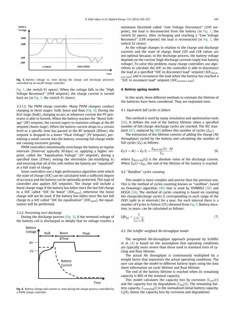
Fig. 3. Battery voltage vs. time during the charge and discharge processescontrolled by an on/off charge controller.

R. Dufo-López et al. / Applied Energy 115 (2014) 242–253 245

Fig. 1, the switch S1 opens). When the voltage falls to the ‘‘HighVoltage Reconnect’’ (HVR setpoint), the charge current is turnedback on (in Fig. 1, the switch S1 closes).

3.3.1.2. The PWM charge controller. Many PWM chargers conductcharging in three stages: bulk, boost and float (Fig. 4). During thefirst stage (bulk), charging occurs at whatever current the PV gen-erator is able to furnish. When the battery reaches the ‘‘Boost Volt-age’’ (BV) setpoint, the current tapers to maintain voltage at the BVsetpoint (boost stage). When the battery current drops to a certainlevel or a specific time has passed in the BV setpoint (BTime), thesetpoint is dropped to a lower ‘‘Float Voltage’’ (FV Setpoint), per-mitting a small current into the battery, ensuring full charge whilenot causing excessive gassing.

PWM controllers intentionally overcharge the battery at regularintervals (EInterval, typically 30 days) or, applying a higher set-point, called the ‘‘Equalisation Voltage’’ (EV setpoint), during aspecified time (ETime), mixing the electrolyte (de-stratifying it)and ensuring that all of the cells within the battery are ‘‘equalised’’at a full state of charge.

Some controllers use a high-performance algorithm with whichthe state of charge (SOC) can be calculated with a sufficient degreeof accuracy and the battery can be optimally protected. This type ofcontroller also applies SOC setpoints. The charge will include aboost charge stage if the battery has fallen since the last full chargeto a SOC called ‘‘SOC for boost’’ (SOCboost), otherwise the boostcharge will not be used. If the battery has fallen since the last fullcharge to a SOC called ‘‘SOC for equalisation’’ (SOCequal), the equal-isation will be performed.

3.3.2. Preventing over-dischargeDuring the discharge process (Fig. 3), if the terminal voltage of

the battery cell is discharged so deeply that its voltage reaches a

Fig. 4. Battery voltage and current vs. time during the charge process controlled bya PWM charge controller.

minimum threshold called ‘‘Low Voltage Disconnect’’ (LVD set-point), the load is disconnected from the battery (in Fig. 1, theswitch S2 opens). After recharging and reaching a ‘‘Low VoltageReconnect’’ (LVR setpoint) the load is reconnected (in Fig. 1, theswitch S2 closes)

As the voltage changes in relation to the charge and dischargecurrents and the state of charge, fixed LVD and LVR values arenot optimal because, in the discharge process, the battery voltagedepends on the current (high discharge currents imply low batteryvoltage). To solve this problem, many charge controllers use algo-rithms to calculate the SOC so the controller is able to disconnectthe load at a specified ‘‘SOC to disconnect load’’ setpoint (SOCdiscon-

nect_load) and it reconnects the load when the battery has reached a‘‘SOC to reconnect load’’ setpoint (SOCreconnect_load).

4. Battery ageing models

In this work, three different methods to estimate the lifetime ofthe batteries have been considered. They are explained next.

4.1. Equivalent full cycles to failure

This method is used by many simulation and optimisation tools[26]. It defines the end of the battery lifetime when a specifiednumber of full charge–discharge cycles are reached. The IEC stan-dard [47], replaced by [48] defines this number of cycles (ZIEC).

The estimation of the lifetime consists of adding the charge (Ahthroughput) cycled by the battery and calculating the number offull cycles (ZN) as follows:

ZNðt þ DtÞ ¼ ZNðtÞ þjIdisch batðtÞj � Dt

CNð6Þ

where |Idisch_bat(t)| is the absolute value of the discharge current.When ZN(t) = ZIEC, the end of the lifetime of the battery is reached.

4.2. ‘‘Rainflow’’ cycles counting

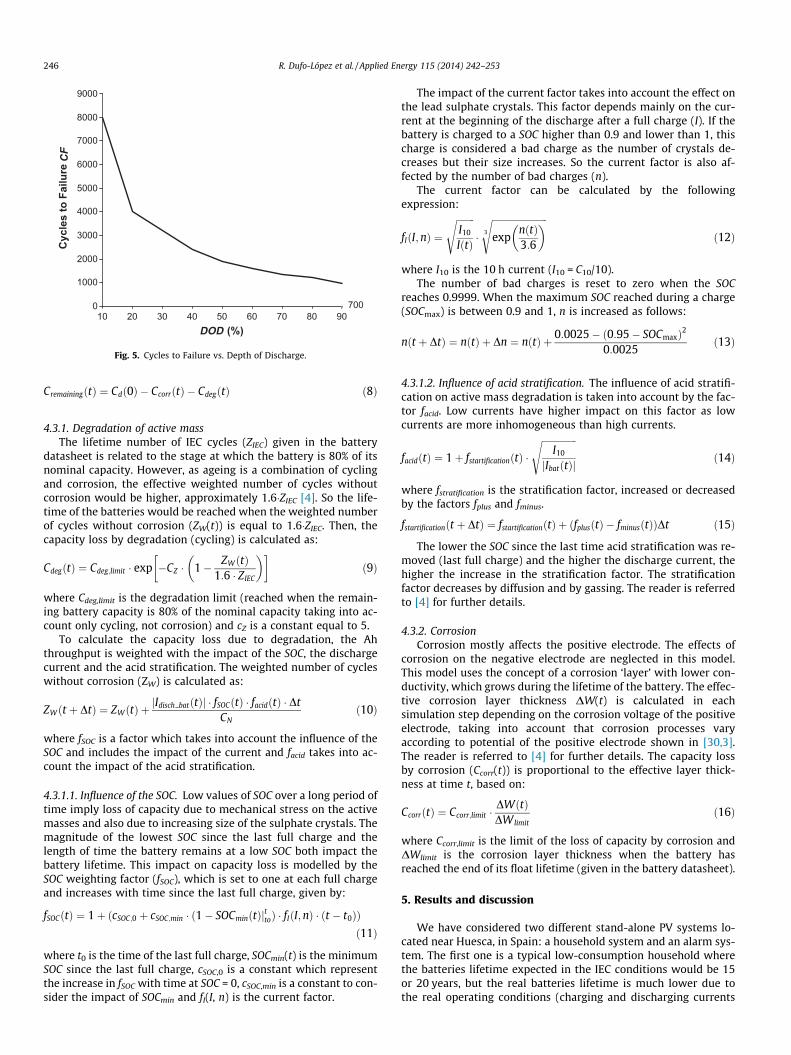
This model is more complex and precise than the previous one.This is the method of cycles counting known as ‘‘rainflow’’, basedon Downing’s algorithm [49] that is used by HYBRID2 [50] andHOGA [26]. The method of cycles counting is based on countingthe charge/discharge cycles Zi corresponding to each range of theDOD (split in m intervals) for a year. For each interval there is anumber of Cycles to Failure (CFi) obtained from Fig. 5. Battery dura-tion, in years, can be calculated as follows:

Lifebat ¼1Pm

i¼1Zi

CFi

ð7Þ

4.3. The Schiffer weighted Ah-throughput model

The weighted Ah-throughput approach proposed by Schifferet al. [4] is based on the assumption that operating conditionsare typically more severe than those used in standard tests of cy-cling and float lifetime.

The actual Ah throughput is continuously multiplied by aweight factor that represents the actual operating conditions. Theuser can adapt the model to different battery types using the datasheet information on cycle lifetime and float lifetime.

The end of the battery lifetime is reached when its remainingcapacity is 80% of the nominal capacity.

This model calculates the capacity loss by corrosion (Ccorr(t))and the capacity loss by degradation (Cdeg(t)). The remaining bat-tery capacity, Cremaining(t) is the normalised initial battery capacity,Cd(0), minus the capacity loss by corrosion and degradation:

0

1000

2000

3000

4000

5000

6000

7000

8000

9000

10 20 30 40 50 60 70 80 90DOD (%)

700

Cyc

les

toFa

ilureCF

Fig. 5. Cycles to Failure vs. Depth of Discharge.

246 R. Dufo-López et al. / Applied Energy 115 (2014) 242–253

CremainingðtÞ ¼ Cdð0Þ � CcorrðtÞ � CdegðtÞ ð8Þ

4.3.1. Degradation of active massThe lifetime number of IEC cycles (ZIEC) given in the battery

datasheet is related to the stage at which the battery is 80% of itsnominal capacity. However, as ageing is a combination of cyclingand corrosion, the effective weighted number of cycles withoutcorrosion would be higher, approximately 1.6�ZIEC [4]. So the life-time of the batteries would be reached when the weighted numberof cycles without corrosion (ZW(t)) is equal to 1.6�ZIEC. Then, thecapacity loss by degradation (cycling) is calculated as:

CdegðtÞ ¼ Cdeg;limit � exp �CZ � 1� ZWðtÞ1:6 � ZIEC

� �� �ð9Þ

where Cdeg,limit is the degradation limit (reached when the remain-ing battery capacity is 80% of the nominal capacity taking into ac-count only cycling, not corrosion) and cZ is a constant equal to 5.

To calculate the capacity loss due to degradation, the Ahthroughput is weighted with the impact of the SOC, the dischargecurrent and the acid stratification. The weighted number of cycleswithout corrosion (ZW) is calculated as:

ZWðt þ DtÞ ¼ ZWðtÞ þjIdisch batðtÞj � fSOCðtÞ � facidðtÞ � Dt

CNð10Þ

where fSOC is a factor which takes into account the influence of theSOC and includes the impact of the current and facid takes into ac-count the impact of the acid stratification.

4.3.1.1. Influence of the SOC. Low values of SOC over a long period oftime imply loss of capacity due to mechanical stress on the activemasses and also due to increasing size of the sulphate crystals. Themagnitude of the lowest SOC since the last full charge and thelength of time the battery remains at a low SOC both impact thebattery lifetime. This impact on capacity loss is modelled by theSOC weighting factor (fSOC), which is set to one at each full chargeand increases with time since the last full charge, given by:

fSOCðtÞ ¼ 1þ ðcSOC;0 þ cSOC;min � ð1� SOCminðtÞjttoÞ � fIðI;nÞ � ðt � t0ÞÞð11Þ

where t0 is the time of the last full charge, SOCmin(t) is the minimumSOC since the last full charge, cSOC,0 is a constant which representthe increase in fSOC with time at SOC = 0, cSOC,min is a constant to con-sider the impact of SOCmin and fI(I, n) is the current factor.

The impact of the current factor takes into account the effect onthe lead sulphate crystals. This factor depends mainly on the cur-rent at the beginning of the discharge after a full charge (I). If thebattery is charged to a SOC higher than 0.9 and lower than 1, thischarge is considered a bad charge as the number of crystals de-creases but their size increases. So the current factor is also af-fected by the number of bad charges (n).

The current factor can be calculated by the followingexpression:

fIðI;nÞ ¼ffiffiffiffiffiffiffiffiI10

IðtÞ

s�

ffiffiffiffiffiffiffiffiffiffiffiffiffiffiffiffiffiffiffiffiffiffiffiffiexp

nðtÞ3:6

� �3

sð12Þ

where I10 is the 10 h current (I10 = C10/10).The number of bad charges is reset to zero when the SOC

reaches 0.9999. When the maximum SOC reached during a charge(SOCmax) is between 0.9 and 1, n is increased as follows:

nðt þ DtÞ ¼ nðtÞ þ Dn ¼ nðtÞ þ 0:0025� ð0:95� SOCmaxÞ2

0:0025ð13Þ

4.3.1.2. Influence of acid stratification. The influence of acid stratifi-cation on active mass degradation is taken into account by the fac-tor facid. Low currents have higher impact on this factor as lowcurrents are more inhomogeneous than high currents.

facidðtÞ ¼ 1þ fstartificationðtÞ �ffiffiffiffiffiffiffiffiffiffiffiffiffiffiffi

I10

jIbatðtÞj

sð14Þ

where fstratification is the stratification factor, increased or decreasedby the factors fplus and fminus.

fstartificationðt þ DtÞ ¼ fstartificationðtÞ þ ðfplusðtÞ � fminusðtÞÞDt ð15Þ

The lower the SOC since the last time acid stratification was re-moved (last full charge) and the higher the discharge current, thehigher the increase in the stratification factor. The stratificationfactor decreases by diffusion and by gassing. The reader is referredto [4] for further details.

4.3.2. CorrosionCorrosion mostly affects the positive electrode. The effects of

corrosion on the negative electrode are neglected in this model.This model uses the concept of a corrosion ‘layer’ with lower con-ductivity, which grows during the lifetime of the battery. The effec-tive corrosion layer thickness DW(t) is calculated in eachsimulation step depending on the corrosion voltage of the positiveelectrode, taking into account that corrosion processes varyaccording to potential of the positive electrode shown in [30,3].The reader is referred to [4] for further details. The capacity lossby corrosion (Ccorr(t)) is proportional to the effective layer thick-ness at time t, based on:

CcorrðtÞ ¼ Ccorr;limit �DWðtÞDWlimit

ð16Þ

where Ccorr,limit is the limit of the loss of capacity by corrosion andDWlimit is the corrosion layer thickness when the battery hasreached the end of its float lifetime (given in the battery datasheet).

5. Results and discussion

We have considered two different stand-alone PV systems lo-cated near Huesca, in Spain: a household system and an alarm sys-tem. The first one is a typical low-consumption household wherethe batteries lifetime expected in the IEC conditions would be 15or 20 years, but the real batteries lifetime is much lower due tothe real operating conditions (charging and discharging currents

050

100150200250300350400450500

0 1000 2000 3000 4000 5000 6000 7000 8000

Load

(W)

Hour

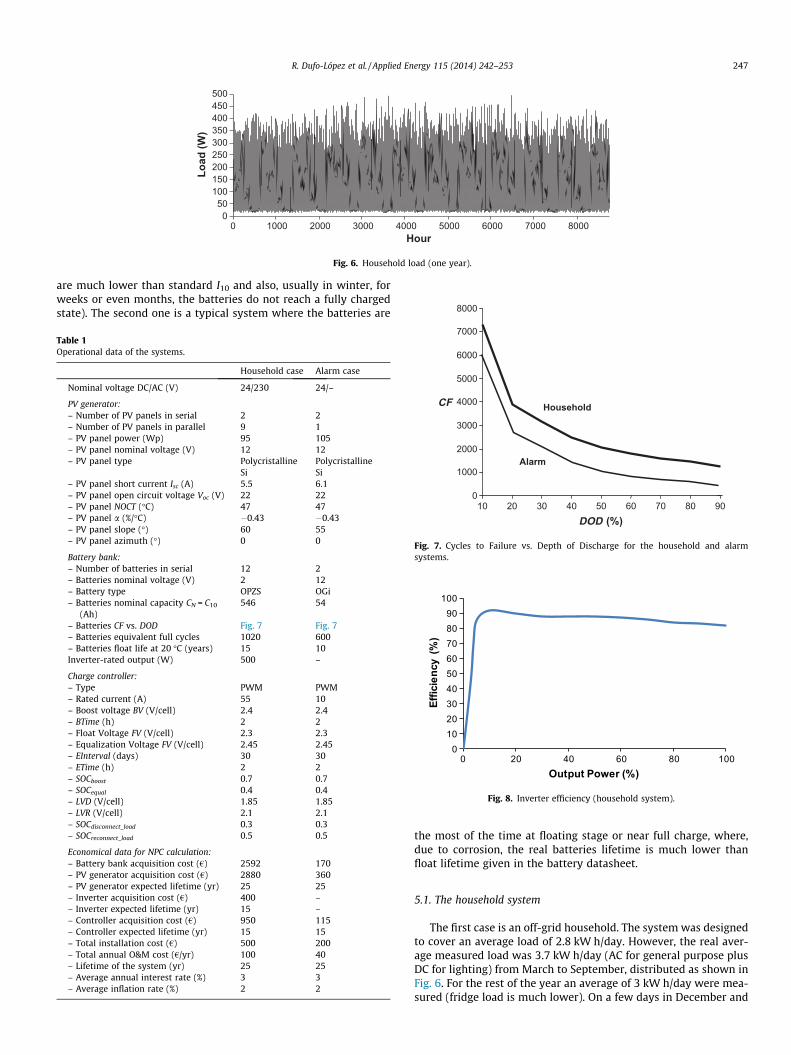
Fig. 6. Household load (one year).

8000

R. Dufo-López et al. / Applied Energy 115 (2014) 242–253 247

are much lower than standard I10 and also, usually in winter, forweeks or even months, the batteries do not reach a fully chargedstate). The second one is a typical system where the batteries are

Table 1Operational data of the systems.

Household case Alarm case

Nominal voltage DC/AC (V) 24/230 24/–

PV generator:– Number of PV panels in serial 2 2– Number of PV panels in parallel 9 1– PV panel power (Wp) 95 105– PV panel nominal voltage (V) 12 12– PV panel type Polycristalline

SiPolycristallineSi

– PV panel short current Isc (A) 5.5 6.1– PV panel open circuit voltage Voc (V) 22 22– PV panel NOCT (�C) 47 47– PV panel a (%/�C) �0.43 �0.43– PV panel slope (�) 60 55– PV panel azimuth (�) 0 0

Battery bank:– Number of batteries in serial 12 2– Batteries nominal voltage (V) 2 12– Battery type OPZS OGi– Batteries nominal capacity CN = C10

(Ah)546 54

– Batteries CF vs. DOD Fig. 7 Fig. 7– Batteries equivalent full cycles 1020 600– Batteries float life at 20 �C (years) 15 10Inverter-rated output (W) 500 –

Charge controller:– Type PWM PWM– Rated current (A) 55 10– Boost voltage BV (V/cell) 2.4 2.4– BTime (h) 2 2– Float Voltage FV (V/cell) 2.3 2.3– Equalization Voltage FV (V/cell) 2.45 2.45– EInterval (days) 30 30– ETime (h) 2 2– SOCboost 0.7 0.7– SOCequal 0.4 0.4– LVD (V/cell) 1.85 1.85– LVR (V/cell) 2.1 2.1– SOCdisconnect_load 0.3 0.3– SOCreconnect_load 0.5 0.5

Economical data for NPC calculation:– Battery bank acquisition cost (€) 2592 170– PV generator acquisition cost (€) 2880 360– PV generator expected lifetime (yr) 25 25– Inverter acquisition cost (€) 400 –– Inverter expected lifetime (yr) 15 –– Controller acquisition cost (€) 950 115– Controller expected lifetime (yr) 15 15– Total installation cost (€) 500 200– Total annual O&M cost (€/yr) 100 40– Lifetime of the system (yr) 25 25– Average annual interest rate (%) 3 3– Average inflation rate (%) 2 2

0

1000

2000

3000

4000

5000

6000

7000

10 20 30 40 50 60 70 80 90DOD (%)

CF Household

Alarm

Fig. 7. Cycles to Failure vs. Depth of Discharge for the household and alarmsystems.

0102030405060708090

100

0 20 40 60 80 100

Effic

ienc

y (%

)

Output Power (%)

Fig. 8. Inverter efficiency (household system).

the most of the time at floating stage or near full charge, where,due to corrosion, the real batteries lifetime is much lower thanfloat lifetime given in the battery datasheet.

5.1. The household system

The first case is an off-grid household. The system was designedto cover an average load of 2.8 kW h/day. However, the real aver-age measured load was 3.7 kW h/day (AC for general purpose plusDC for lighting) from March to September, distributed as shown inFig. 6. For the rest of the year an average of 3 kW h/day were mea-sured (fridge load is much lower). On a few days in December and

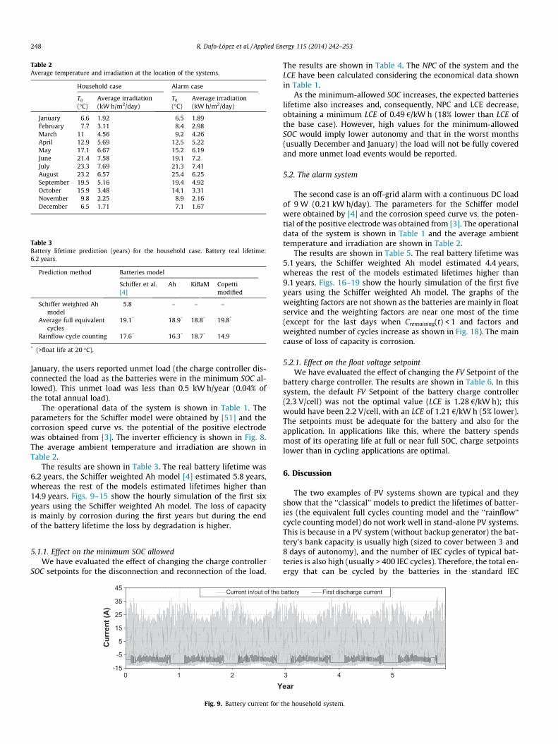
Table 2Average temperature and irradiation at the location of the systems.

Household case Alarm case

Ta

(�C)Average irradiation(kW h/m2/day)

Ta

(�C)Average irradiation(kW h/m2/day)

January 6.6 1.92 6.5 1.89February 7.7 3.11 8.4 2.98March 11 4.56 9.2 4.26April 12.9 5.69 12.5 5.22May 17.1 6.67 15.2 6.19June 21.4 7.58 19.1 7.2July 23.3 7.69 21.3 7.41August 23.2 6.57 25.4 6.25September 19.5 5.16 19.4 4.92October 15.9 3.48 14.1 3.31November 9.8 2.25 8.9 2.16December 6.5 1.71 7.1 1.67

Table 3Battery lifetime prediction (years) for the household case. Battery real lifetime:6.2 years.

Prediction method Batteries model

Schiffer et al.[4]

Ah KiBaM Copettimodified

Schiffer weighted Ahmodel

5.8 – – –

Average full equivalentcycles

19.1* 18.9* 18.8* 19.8*

Rainflow cycle counting 17.6* 16.3* 18.7* 14.9

* (>float life at 20 �C).

248 R. Dufo-López et al. / Applied Energy 115 (2014) 242–253

January, the users reported unmet load (the charge controller dis-connected the load as the batteries were in the minimum SOC al-lowed). This unmet load was less than 0.5 kW h/year (0.04% ofthe total annual load).

The operational data of the system is shown in Table 1. Theparameters for the Schiffer model were obtained by [51] and thecorrosion speed curve vs. the potential of the positive electrodewas obtained from [3]. The inverter efficiency is shown in Fig. 8.The average ambient temperature and irradiation are shown inTable 2.

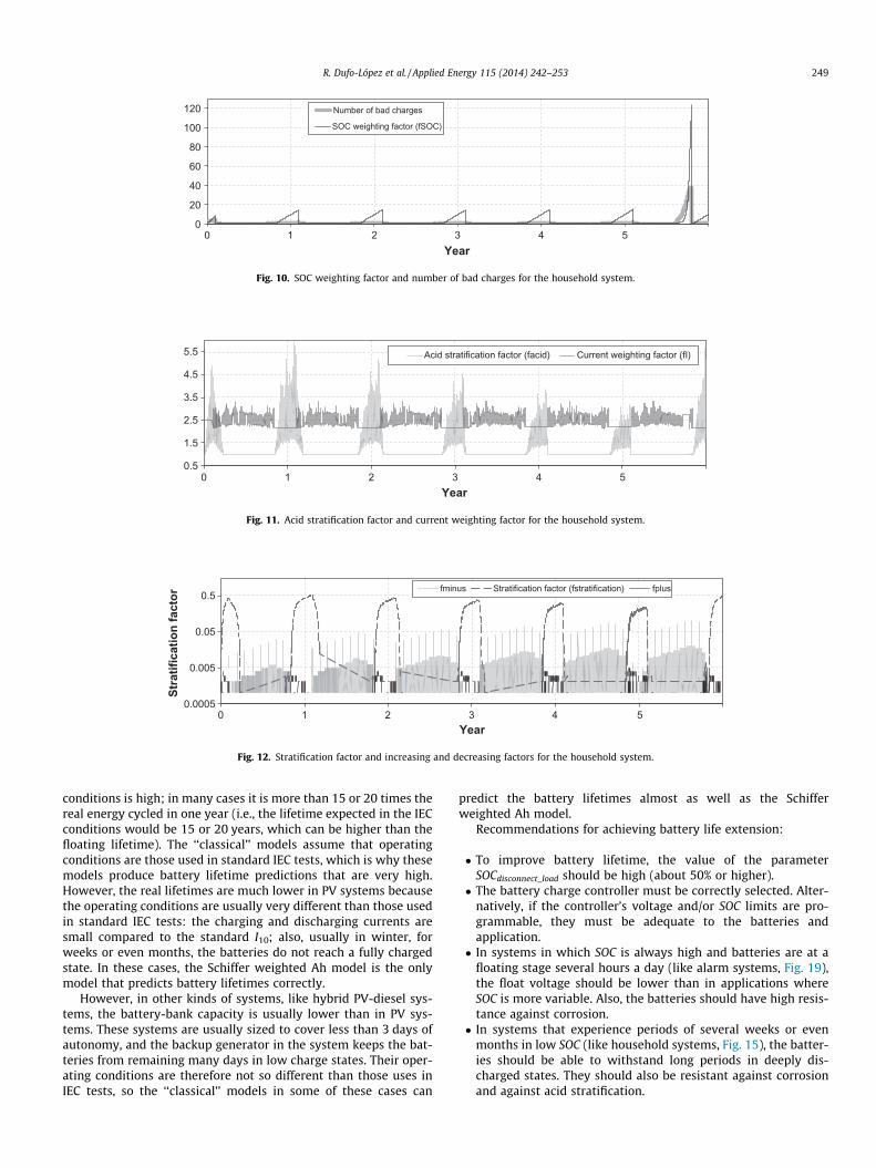
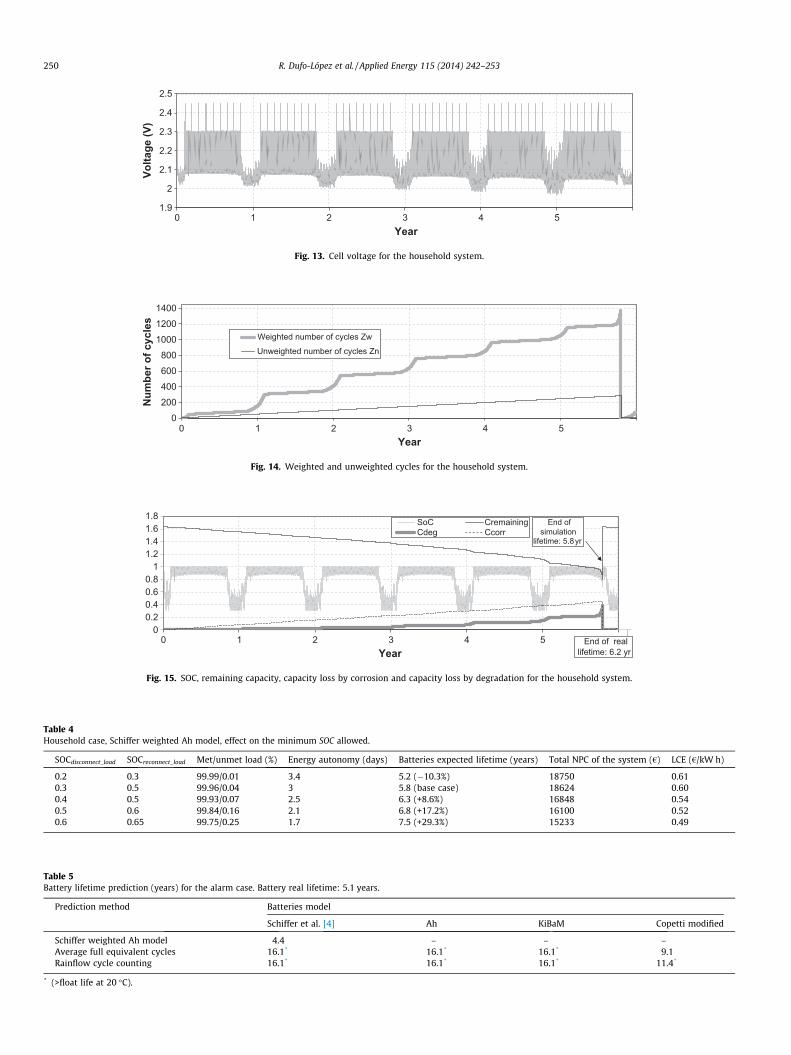
The results are shown in Table 3. The real battery lifetime was6.2 years, the Schiffer weighted Ah model [4] estimated 5.8 years,whereas the rest of the models estimated lifetimes higher than14.9 years. Figs. 9–15 show the hourly simulation of the first sixyears using the Schiffer weighted Ah model. The loss of capacityis mainly by corrosion during the first years but during the endof the battery lifetime the loss by degradation is higher.

5.1.1. Effect on the minimum SOC allowedWe have evaluated the effect of changing the charge controller

SOC setpoints for the disconnection and reconnection of the load.

-15

-5

5

15

25

35

45

0 1 2

Cur

rent

(A)

Y

Current in/out of the

Fig. 9. Battery current for t

The results are shown in Table 4. The NPC of the system and theLCE have been calculated considering the economical data shownin Table 1.

As the minimum-allowed SOC increases, the expected batterieslifetime also increases and, consequently, NPC and LCE decrease,obtaining a minimum LCE of 0.49 €/kW h (18% lower than LCE ofthe base case). However, high values for the minimum-allowedSOC would imply lower autonomy and that in the worst months(usually December and January) the load will not be fully coveredand more unmet load events would be reported.

5.2. The alarm system

The second case is an off-grid alarm with a continuous DC loadof 9 W (0.21 kW h/day). The parameters for the Schiffer modelwere obtained by [4] and the corrosion speed curve vs. the poten-tial of the positive electrode was obtained from [3]. The operationaldata of the system is shown in Table 1 and the average ambienttemperature and irradiation are shown in Table 2.

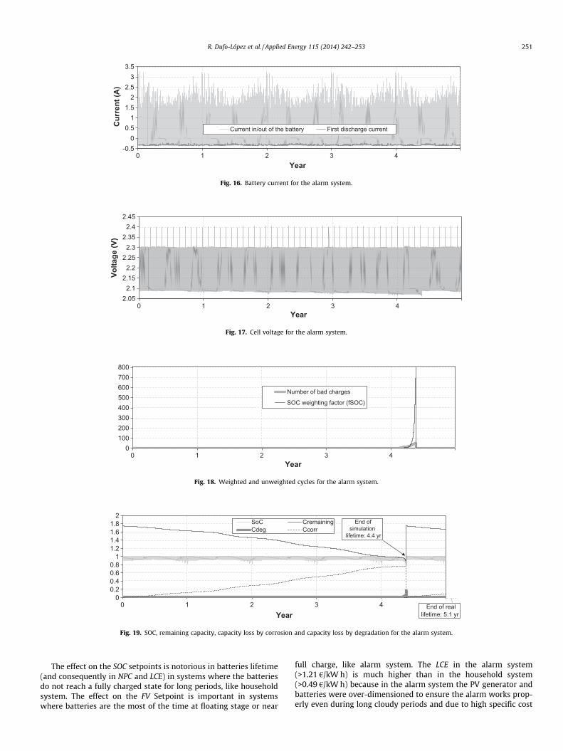
The results are shown in Table 5. The real battery lifetime was5.1 years, the Schiffer weighted Ah model estimated 4.4 years,whereas the rest of the models estimated lifetimes higher than9.1 years. Figs. 16–19 show the hourly simulation of the first fiveyears using the Schiffer weighted Ah model. The graphs of theweighting factors are not shown as the batteries are mainly in floatservice and the weighting factors are near one most of the time(except for the last days when Cremaining(t) < 1 and factors andweighted number of cycles increase as shown in Fig. 18). The maincause of loss of capacity is corrosion.

5.2.1. Effect on the float voltage setpointWe have evaluated the effect of changing the FV Setpoint of the

battery charge controller. The results are shown in Table 6. In thissystem, the default FV Setpoint of the battery charge controller(2.3 V/cell) was not the optimal value (LCE is 1.28 €/kW h); thiswould have been 2.2 V/cell, with an LCE of 1.21 €/kW h (5% lower).The setpoints must be adequate for the battery and also for theapplication. In applications like this, where the battery spendsmost of its operating life at full or near full SOC, charge setpointslower than in cycling applications are optimal.

6. Discussion

The two examples of PV systems shown are typical and theyshow that the ‘‘classical’’ models to predict the lifetimes of batter-ies (the equivalent full cycles counting model and the ‘‘rainflow’’cycle counting model) do not work well in stand-alone PV systems.This is because in a PV system (without backup generator) the bat-tery’s bank capacity is usually high (sized to cover between 3 and8 days of autonomy), and the number of IEC cycles of typical bat-teries is also high (usually > 400 IEC cycles). Therefore, the total en-ergy that can be cycled by the batteries in the standard IEC

3 4 5

ear

battery First discharge current

he household system.

0

20

40

60

80

100

120

0 1 2 3 4 5Year

Number of bad charges

SOC weighting factor (fSOC)

Fig. 10. SOC weighting factor and number of bad charges for the household system.

0.5

1.5

2.5

3.5

4.5

5.5

0 1 2 3 4 5Year

Acid stratification factor (facid) Current weighting factor (fI)

Fig. 11. Acid stratification factor and current weighting factor for the household system.

0.0005

0.005

0.05

0.5

0 1 2 3 4 5

Stra

tific

atio

n fa

ctor

Year

fminus Stratification factor (fstratification) fplus

Fig. 12. Stratification factor and increasing and decreasing factors for the household system.

R. Dufo-López et al. / Applied Energy 115 (2014) 242–253 249

conditions is high; in many cases it is more than 15 or 20 times thereal energy cycled in one year (i.e., the lifetime expected in the IECconditions would be 15 or 20 years, which can be higher than thefloating lifetime). The ‘‘classical’’ models assume that operatingconditions are those used in standard IEC tests, which is why thesemodels produce battery lifetime predictions that are very high.However, the real lifetimes are much lower in PV systems becausethe operating conditions are usually very different than those usedin standard IEC tests: the charging and discharging currents aresmall compared to the standard I10; also, usually in winter, forweeks or even months, the batteries do not reach a fully chargedstate. In these cases, the Schiffer weighted Ah model is the onlymodel that predicts battery lifetimes correctly.

However, in other kinds of systems, like hybrid PV-diesel sys-tems, the battery-bank capacity is usually lower than in PV sys-tems. These systems are usually sized to cover less than 3 days ofautonomy, and the backup generator in the system keeps the bat-teries from remaining many days in low charge states. Their oper-ating conditions are therefore not so different than those uses inIEC tests, so the ‘‘classical’’ models in some of these cases can

predict the battery lifetimes almost as well as the Schifferweighted Ah model.

Recommendations for achieving battery life extension:

� To improve battery lifetime, the value of the parameterSOCdisconnect_load should be high (about 50% or higher).� The battery charge controller must be correctly selected. Alter-

natively, if the controller’s voltage and/or SOC limits are pro-grammable, they must be adequate to the batteries andapplication.� In systems in which SOC is always high and batteries are at a

floating stage several hours a day (like alarm systems, Fig. 19),the float voltage should be lower than in applications whereSOC is more variable. Also, the batteries should have high resis-tance against corrosion.� In systems that experience periods of several weeks or even

months in low SOC (like household systems, Fig. 15), the batter-ies should be able to withstand long periods in deeply dis-charged states. They should also be resistant against corrosionand against acid stratification.

1.9

2

2.1

2.2

2.3

2.4

2.5

0 1 2 3 4 5

Volta

ge (V

)

Year

Fig. 13. Cell voltage for the household system.

0200400600800

100012001400

0 1 2 3 4 5

Num

ber o

f cyc

les

Year

Weighted number of cycles Zw

Unweighted number of cycles Zn

Fig. 14. Weighted and unweighted cycles for the household system.

00.20.40.60.8

11.21.41.61.8

0 1 2 3 4 5Year

SoC CremainingCdeg Ccorr

End of simulation

lifetime: 5.8yr

End of real lifetime: 6.2 yr

Fig. 15. SOC, remaining capacity, capacity loss by corrosion and capacity loss by degradation for the household system.

Table 4Household case, Schiffer weighted Ah model, effect on the minimum SOC allowed.

SOCdisconnect_load SOCreconnect_load Met/unmet load (%) Energy autonomy (days) Batteries expected lifetime (years) Total NPC of the system (€) LCE (€/kW h)

0.2 0.3 99.99/0.01 3.4 5.2 (�10.3%) 18750 0.610.3 0.5 99.96/0.04 3 5.8 (base case) 18624 0.600.4 0.5 99.93/0.07 2.5 6.3 (+8.6%) 16848 0.540.5 0.6 99.84/0.16 2.1 6.8 (+17.2%) 16100 0.520.6 0.65 99.75/0.25 1.7 7.5 (+29.3%) 15233 0.49

Table 5Battery lifetime prediction (years) for the alarm case. Battery real lifetime: 5.1 years.

Prediction method Batteries model

Schiffer et al. [4] Ah KiBaM Copetti modified

Schiffer weighted Ah model 4.4 – – –Average full equivalent cycles 16.1* 16.1* 16.1* 9.1Rainflow cycle counting 16.1* 16.1* 16.1* 11.4*

* (>float life at 20 �C).

250 R. Dufo-López et al. / Applied Energy 115 (2014) 242–253

-0.50

0.51

1.52

2.53

3.5

0 1 2 3 4

Cur

rent

(A)

Year

Current in/out of the battery First discharge current

Fig. 16. Battery current for the alarm system.

2.052.1

2.152.2

2.252.3

2.352.4

2.45

0 1 2 3 4

Volta

ge (V

)

Year

Fig. 17. Cell voltage for the alarm system.

0100200300400500600700800

0 1 2 3 4Year

Number of bad charges

SOC weighting factor (fSOC)

Fig. 18. Weighted and unweighted cycles for the alarm system.

00.20.40.60.8

11.21.41.61.8

2

0 1 2 3 4Year

SoC CremainingCdeg Ccorr

End of simulation

lifetime: 4.4 yr

End of real lifetime: 5.1 yr

Fig. 19. SOC, remaining capacity, capacity loss by corrosion and capacity loss by degradation for the alarm system.

R. Dufo-López et al. / Applied Energy 115 (2014) 242–253 251

The effect on the SOC setpoints is notorious in batteries lifetime(and consequently in NPC and LCE) in systems where the batteriesdo not reach a fully charged state for long periods, like householdsystem. The effect on the FV Setpoint is important in systemswhere batteries are the most of the time at floating stage or near

full charge, like alarm system. The LCE in the alarm system(>1.21 €/kW h) is much higher than in the household system(>0.49 €/kW h) because in the alarm system the PV generator andbatteries were over-dimensioned to ensure the alarm works prop-erly even during long cloudy periods and due to high specific cost

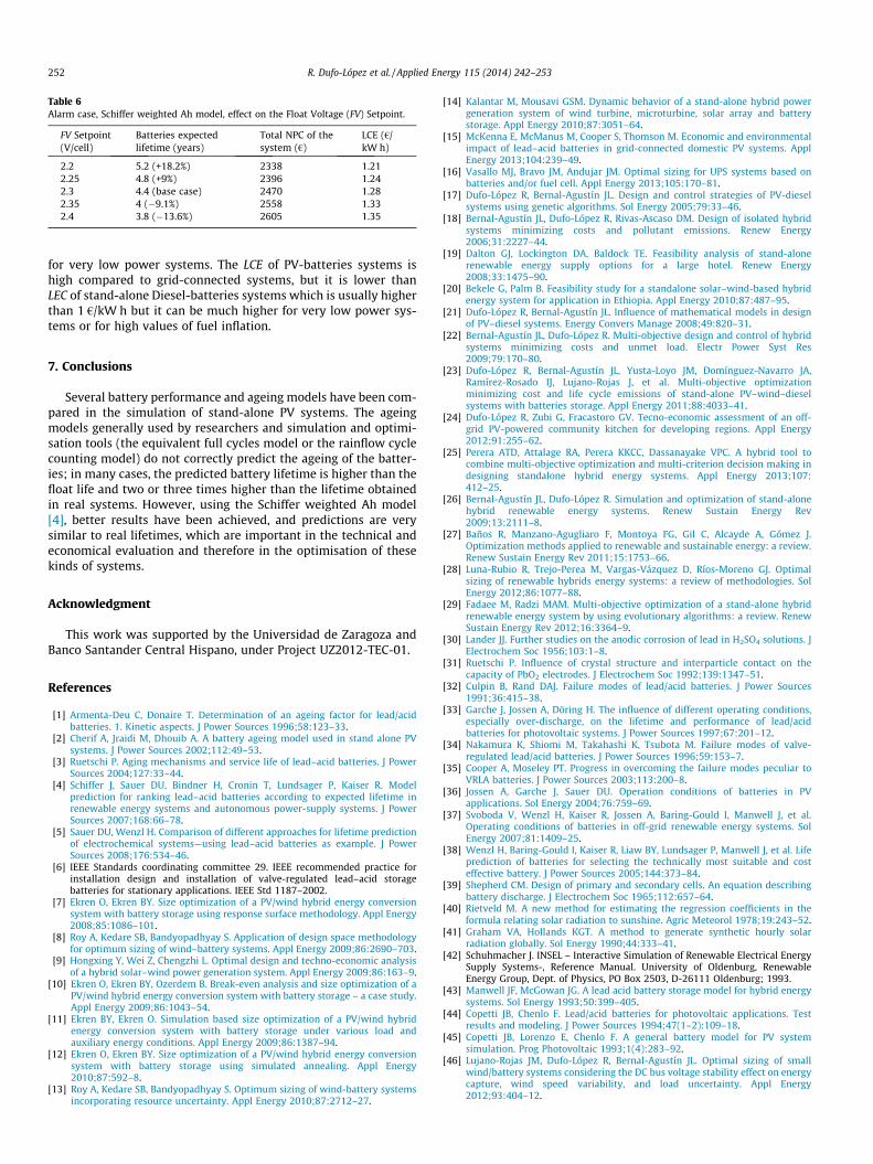
Table 6Alarm case, Schiffer weighted Ah model, effect on the Float Voltage (FV) Setpoint.

FV Setpoint(V/cell)

Batteries expectedlifetime (years)

Total NPC of thesystem (€)

LCE (€/kW h)

2.2 5.2 (+18.2%) 2338 1.212.25 4.8 (+9%) 2396 1.242.3 4.4 (base case) 2470 1.282.35 4 (�9.1%) 2558 1.332.4 3.8 (�13.6%) 2605 1.35

252 R. Dufo-López et al. / Applied Energy 115 (2014) 242–253

for very low power systems. The LCE of PV-batteries systems ishigh compared to grid-connected systems, but it is lower thanLEC of stand-alone Diesel-batteries systems which is usually higherthan 1 €/kW h but it can be much higher for very low power sys-tems or for high values of fuel inflation.

7. Conclusions

Several battery performance and ageing models have been com-pared in the simulation of stand-alone PV systems. The ageingmodels generally used by researchers and simulation and optimi-sation tools (the equivalent full cycles model or the rainflow cyclecounting model) do not correctly predict the ageing of the batter-ies; in many cases, the predicted battery lifetime is higher than thefloat life and two or three times higher than the lifetime obtainedin real systems. However, using the Schiffer weighted Ah model[4], better results have been achieved, and predictions are verysimilar to real lifetimes, which are important in the technical andeconomical evaluation and therefore in the optimisation of thesekinds of systems.

Acknowledgment

This work was supported by the Universidad de Zaragoza andBanco Santander Central Hispano, under Project UZ2012-TEC-01.

References

[1] Armenta-Deu C, Donaire T. Determination of an ageing factor for lead/acidbatteries. 1. Kinetic aspects. J Power Sources 1996;58:123–33.

[2] Cherif A, Jraidi M, Dhouib A. A battery ageing model used in stand alone PVsystems. J Power Sources 2002;112:49–53.

[3] Ruetschi P. Aging mechanisms and service life of lead–acid batteries. J PowerSources 2004;127:33–44.

[4] Schiffer J, Sauer DU, Bindner H, Cronin T, Lundsager P, Kaiser R. Modelprediction for ranking lead–acid batteries according to expected lifetime inrenewable energy systems and autonomous power-supply systems. J PowerSources 2007;168:66–78.

[5] Sauer DU, Wenzl H. Comparison of different approaches for lifetime predictionof electrochemical systems—using lead–acid batteries as example. J PowerSources 2008;176:534–46.

[6] IEEE Standards coordinating committee 29. IEEE recommended practice forinstallation design and installation of valve-regulated lead–acid storagebatteries for stationary applications. IEEE Std 1187–2002.

[7] Ekren O, Ekren BY. Size optimization of a PV/wind hybrid energy conversionsystem with battery storage using response surface methodology. Appl Energy2008;85:1086–101.

[8] Roy A, Kedare SB, Bandyopadhyay S. Application of design space methodologyfor optimum sizing of wind–battery systems. Appl Energy 2009;86:2690–703.

[9] Hongxing Y, Wei Z, Chengzhi L. Optimal design and techno-economic analysisof a hybrid solar–wind power generation system. Appl Energy 2009;86:163–9.

[10] Ekren O, Ekren BY, Ozerdem B. Break-even analysis and size optimization of aPV/wind hybrid energy conversion system with battery storage – a case study.Appl Energy 2009;86:1043–54.

[11] Ekren BY, Ekren O. Simulation based size optimization of a PV/wind hybridenergy conversion system with battery storage under various load andauxiliary energy conditions. Appl Energy 2009;86:1387–94.

[12] Ekren O, Ekren BY. Size optimization of a PV/wind hybrid energy conversionsystem with battery storage using simulated annealing. Appl Energy2010;87:592–8.

[13] Roy A, Kedare SB, Bandyopadhyay S. Optimum sizing of wind-battery systemsincorporating resource uncertainty. Appl Energy 2010;87:2712–27.

[14] Kalantar M, Mousavi GSM. Dynamic behavior of a stand-alone hybrid powergeneration system of wind turbine, microturbine, solar array and batterystorage. Appl Energy 2010;87:3051–64.

[15] McKenna E, McManus M, Cooper S, Thomson M. Economic and environmentalimpact of lead–acid batteries in grid-connected domestic PV systems. ApplEnergy 2013;104:239–49.

[16] Vasallo MJ, Bravo JM, Andujar JM. Optimal sizing for UPS systems based onbatteries and/or fuel cell. Appl Energy 2013;105:170–81.

[17] Dufo-López R, Bernal-Agustín JL. Design and control strategies of PV-dieselsystems using genetic algorithms. Sol Energy 2005;79:33–46.

[18] Bernal-Agustín JL, Dufo-López R, Rivas-Ascaso DM. Design of isolated hybridsystems minimizing costs and pollutant emissions. Renew Energy2006;31:2227–44.

[19] Dalton GJ, Lockington DA, Baldock TE. Feasibility analysis of stand-alonerenewable energy supply options for a large hotel. Renew Energy2008;33:1475–90.

[20] Bekele G, Palm B. Feasibility study for a standalone solar–wind-based hybridenergy system for application in Ethiopia. Appl Energy 2010;87:487–95.

[21] Dufo-López R, Bernal-Agustín JL. Influence of mathematical models in designof PV–diesel systems. Energy Convers Manage 2008;49:820–31.

[22] Bernal-Agustín JL, Dufo-López R. Multi-objective design and control of hybridsystems minimizing costs and unmet load. Electr Power Syst Res2009;79:170–80.

[23] Dufo-López R, Bernal-Agustín JL, Yusta-Loyo JM, Domínguez-Navarro JA,Ramírez-Rosado IJ, Lujano-Rojas J, et al. Multi-objective optimizationminimizing cost and life cycle emissions of stand-alone PV–wind–dieselsystems with batteries storage. Appl Energy 2011;88:4033–41.

[24] Dufo-López R, Zubi G, Fracastoro GV. Tecno-economic assessment of an off-grid PV-powered community kitchen for developing regions. Appl Energy2012;91:255–62.

[25] Perera ATD, Attalage RA, Perera KKCC, Dassanayake VPC. A hybrid tool tocombine multi-objective optimization and multi-criterion decision making indesigning standalone hybrid energy systems. Appl Energy 2013;107:412–25.

[26] Bernal-Agustín JL, Dufo-López R. Simulation and optimization of stand-alonehybrid renewable energy systems. Renew Sustain Energy Rev2009;13:2111–8.

[27] Baños R, Manzano-Agugliaro F, Montoya FG, Gil C, Alcayde A, Gómez J.Optimization methods applied to renewable and sustainable energy: a review.Renew Sustain Energy Rev 2011;15:1753–66.

[28] Luna-Rubio R, Trejo-Perea M, Vargas-Vázquez D, Ríos-Moreno GJ. Optimalsizing of renewable hybrids energy systems: a review of methodologies. SolEnergy 2012;86:1077–88.

[29] Fadaee M, Radzi MAM. Multi-objective optimization of a stand-alone hybridrenewable energy system by using evolutionary algorithms: a review. RenewSustain Energy Rev 2012;16:3364–9.

[30] Lander JJ. Further studies on the anodic corrosion of lead in H2SO4 solutions. JElectrochem Soc 1956;103:1–8.

[31] Ruetschi P. Influence of crystal structure and interparticle contact on thecapacity of PbO2 electrodes. J Electrochem Soc 1992;139:1347–51.

[32] Culpin B, Rand DAJ. Failure modes of lead/acid batteries. J Power Sources1991;36:415–38.

[33] Garche J, Jossen A, Döring H. The influence of different operating conditions,especially over-discharge, on the lifetime and performance of lead/acidbatteries for photovoltaic systems. J Power Sources 1997;67:201–12.

[34] Nakamura K, Shiomi M, Takahashi K, Tsubota M. Failure modes of valve-regulated lead/acid batteries. J Power Sources 1996;59:153–7.

[35] Cooper A, Moseley PT. Progress in overcoming the failure modes peculiar toVRLA batteries. J Power Sources 2003;113:200–8.

[36] Jossen A, Garche J, Sauer DU. Operation conditions of batteries in PVapplications. Sol Energy 2004;76:759–69.

[37] Svoboda V, Wenzl H, Kaiser R, Jossen A, Baring-Gould I, Manwell J, et al.Operating conditions of batteries in off-grid renewable energy systems. SolEnergy 2007;81:1409–25.

[38] Wenzl H, Baring-Gould I, Kaiser R, Liaw BY, Lundsager P, Manwell J, et al. Lifeprediction of batteries for selecting the technically most suitable and costeffective battery. J Power Sources 2005;144:373–84.

[39] Shepherd CM. Design of primary and secondary cells. An equation describingbattery discharge. J Electrochem Soc 1965;112:657–64.

[40] Rietveld M. A new method for estimating the regression coefficients in theformula relating solar radiation to sunshine. Agric Meteorol 1978;19:243–52.

[41] Graham VA, Hollands KGT. A method to generate synthetic hourly solarradiation globally. Sol Energy 1990;44:333–41.

[42] Schuhmacher J. INSEL – Interactive Simulation of Renewable Electrical EnergySupply Systems-, Reference Manual. University of Oldenburg, RenewableEnergy Group, Dept. of Physics, PO Box 2503, D-26111 Oldenburg; 1993.

[43] Manwell JF, McGowan JG. A lead acid battery storage model for hybrid energysystems. Sol Energy 1993;50:399–405.

[44] Copetti JB, Chenlo F. Lead/acid batteries for photovoltaic applications. Testresults and modeling. J Power Sources 1994;47(1–2):109–18.

[45] Copetti JB, Lorenzo E, Chenlo F. A general battery model for PV systemsimulation. Prog Photovoltaic 1993;1(4):283–92.

[46] Lujano-Rojas JM, Dufo-López R, Bernal-Agustín JL. Optimal sizing of smallwind/battery systems considering the DC bus voltage stability effect on energycapture, wind speed variability, and load uncertainty. Appl Energy2012;93:404–12.

R. Dufo-López et al. / Applied Energy 115 (2014) 242–253 253

[47] IEC 60896-1:1987 Stationary lead–acid batteries. General requirements andmethods of test. Vented types.

[48] EN 60896-11:2003. Stationary lead–acid batteries. General requirements andmethods of test. Vented types. General requirements and methods of tests.

[49] Downing SD, Socie DF. Simple rainflow counting algorithms. Int J Fatigue1982;4:31–40.

[50] Green HJ, Manwell J. HYBRID2 – A Versatile Model of the Performance ofHybrid Power Systems. In: Proceedings of WindPower’95, Washington DC,March 27–30, 1995.

[51] Bindner H, Cronin T, Lundsager P, Manwell JF, Abdulwahid U, Baring-Gould I.Lifetime Modelling of lead acid batteries. Denmark National Laboratory Risø;2005.