energies

Article

Comparison of Different Hydraulic FracturingScenarios in Horizontal Wells Using XFEM Based onthe Cohesive Zone Method

Jianxiong Li 1 , Wen Xiao 2, Guanzhong Hao 3, Shiming Dong 1,* , Wen Hua 1,*and Xiaolong Li 4

1 Key Laboratory Deep Underground Science and Engineering, Ministry of Education,College of Architecture and Environment, Sichuan University, Chengdu 610065, China;jianxiongml@126.com

2 Petroleum Engineering Technology Institute of Shengli Oilfield, Dongying 257000, China;xiaow0811@163.com

3 Institute of Gas Recovering Technology in Changqing Oilfield Company Gas Production Plant NO.1,Yulin 718500, China; haoguanzhong901010@gmail.com

4 Sinopec Petroleum Exploration and Production Research Institute, Beijing 100083, China;lixl2018.syky@sinopec.com

* Correspondence: smdong@scu.edu.cn (S.D.); wenhua@scu.edu.cn (W.H.); Tel.: +86-28-85416486 (S.D.)

Received: 6 March 2019; Accepted: 26 March 2019; Published: 31 March 2019�����������������

Abstract: Multistage hydraulic fracturing is a highly effective method for creating multiple transversefractures to improve gas and oil reservoir production. It is critical to minimize the fracture spacingwhile also ensuring transverse propagation of fractures in multi-fractured horizontal wells. In thispaper, a 3D fully coupled pore pressure-stress model based on the extended finite element method(XFEM) combined with the cohesive zone method is established to simulate five different fracturingscenarios in close spacing. The sensitivity of mesh size and the integration method are optimal,which are verified by the highly accurate traditional cohesive zone method. Then, the effect of fivedifferent fracturing scenarios on fracture geometries is compared. It is shown that spacing is a keyparameter controlling fracture geometries in all fracturing scenarios. Alternative sequential andmodified two-step fracturing can significantly reduce the influence of stress shadowing to generatemore transverse fractures and form longer effective fractures. The sequential and two-step fracturingsee an obvious improvement with increased fracture effective length when the spacing increases.The simultaneous fracturing technique can result in excessive closure of the middle fractures, whichcauses serious insertion of proppants. These results offer a new insight on optimization of hydraulicfracturing and can be a guidance for typical field cases.

Keywords: different fracturing scenarios; XFEM; cohesive zone method; close spacing; stress shadowing

1. Introduction

Unconventional reservoirs have ultralow permeability and porosity and often the stimulatedreservoir volumes need to be increased to achieve commercial production rates. Multistage hydraulicfracturing in horizontal wells is a highly effective treatment for enhancing permeability, whichplaces multiple transverse fractures along a horizontal well. When designing the fracturing scenario,it is important to minimize the spacing between clusters for higher production [1,2]. However,closely-spaced clusters may have excessive interactions between fractures, which may result inundesirable fracture propagation patterns [3]. The mechanical interaction between multiple fracturesarises from a fracture’s “stress shadowing” effect, which is mainly determined by the net pressure

Energies 2019, 12, 1232; doi:10.3390/en12071232 www.mdpi.com/journal/energies

Energies 2019, 12, 1232 2 of 19

and the opening of propped fractures. Hence, great attention should be paid on the optimizedtrajectories of transverse fractures and to avoid excessive interference of stress. However, differenthydraulic fracturing scenarios would redistribute the stress field and generate a variety of fracturenetworks. The mechanical mechanism needs a quantitative description with different hydraulicfracturing scenarios, in order to avoid undesirable diversion of fractures.

Due to the complex propagation patterns of fracture networks, it is difficult to measure thegeometry of fractures in field applications using diagnostic techniques. Therefore, numericalsimulations have become an important tool to solve this complex multiple field coupling problem.The problems associated with modeling multistage hydraulic fractures in horizontal wells have beenaddressed by many papers in recent years. By using an analytical solution, Solima et al. studiedthe effect of multiple fractured-induced interference, which would result in an increase in fracturingpressure [4]. Wu and Olson developed a displacement discontinuity method (DDM) to simulatethe propagation of multiple, potential, non-transverse fractures [5]. This model couples the fracturedeformation with fluid flow and can present the interaction effect between multiple fractures. Zou et al.simulated the arbitrary propagation of hydraulic fractures in naturally fractured formations, usingthe discrete element method (DEM) [6]. In order to identify the plastic zone and the softening effecton fracture tips, Haddad et al. developed a finite element method (FEM) based on the cohesive zonemethod (CZM) to investigate the stress interference between horizontal clusters [7]. The extend finiteelement method (XFEM) had been proposed to simulate the fracture propagation along arbitrarypaths, which can be presented without the limitation of element re-meshing [8,9]. This method addsthe special shape function to the standard finite approximation with the framework of partition ofunity. By adding “edge” phantom nodes with pore pressure degrees of freedom, the so alled XFEMbased on CZM can be extended to simulate the hydraulic fracturing problems [10]. Compared tothe recent models for simulating multistage hydraulic fracturing in horizontal wells, this methodprovides the following improvements [11]: (1) fully coupled pore pressure-stress analysis and theeffect of fractured-induced changes can be studied; (2) the leak-off behaviors are incorporated basedon the fluid continuity and coupled with matrix deformations; and (3) more plausible modeling ofquasi-brittle and heterogeneous reservoirs.

In the process of multistage hydraulic fracturing, the in-situ stress and cluster spacing play avital role in creating fracture networks [12]. Therefore, most studies focus on the optimization ofthe cluster spacing, which can avoid the stress interference from multiple fractures. Haddad et al.demonstrated the superiority of simultaneous fracturing to achieve the best fracture geometry byusing the XFEM model. The study verified the strong interference of fractured-induced stress in aclosely-spacing model [10]. Liu et al. developed a XFEM model to investigate the sequential andsimultaneous fracturing in a horizontal well, and the optimal spacing to create a large fracture networkfield was provided [13]. Wang et al. studied the different propagation patterns of sequential andalternative sequential fracturing in horizontal wells [1]. The XFEM model presents the stress orientationcaused by the non-transverse fractures and describes the opening behaviors of propped hydraulicfractures. All the studies described above show that the complex interactions between fracturesand different fracturing scenarios can result in different geometry of fractures. However, it is also achallenge for practical field applications without a clear understanding and optimization of differentfracturing scenarios.

In this paper, a three dimensional (3D) model is developed to simulate nonplanar propagation offractures in the porous media, which uses the XFEM method based on the CZM. Both pore-elasticityand seepage of rock matrix are taken into consideration. This model also allows us to simulate theleak-off between fracture surface and deformations. The mechanical interaction of propped fractures issimulated with five different types of fracturing scenarios: (1) simultaneous fracturing, (2) sequentialfracturing, (3) alternative sequential fracturing, (4) two-step fracturing, and (5) modified two-stepfracturing. The fracture network is characterized in a low in-situ stress scenario and uses close spacing.

Energies 2019, 12, 1232 3 of 19

The optimal scenario is achieved by calculating the whole effective length of fracture network andcomparing the geometries of each fracture network.

2. Modeling and Simulation Method

2.1. Fluid-solid Coupling Equation of Rock

In this simulation, the characteristic of seepage-stress is fully coupled, in which the fluid diffusionin porous medium is taken into account. Only a single phase of fluid is saturated in the pores of rock.The total stress can be determined by the effective stress by the rock skeleton and the pore pressure.According to the principle of virtual work, the equilibrium equation can be written as follows [14]:∫

(σ− pwI)δεdV =∫

St · δvdS +

∫V

f · δvdV (1)

where the σ and pw are the effective stress and pore pressure, respectively; δε and δv are the virtualstrain state and virtual velocity of deformation, respectively; t and f are the surface traction per unitarea and body force per unit volume, respectively; I is the unit matrix.

Fluid flow is simulated in the porous medium according to the continuity equation of liquid flow.The seepage behavior satisfies the typical Darcy’s law. Therefore, the total change of fluid mass equalsto the fluid mass crossing the porous medium per unit time. The continuity equation can be describedas follows [15]:

1J

∂

∂t(Jρwnw) +

∂

∂x(ρwnwvw) = 0 (2)

where the J is the change ratio of porous media; ρw, nw and vw are the mass density of liquid, porosityof medium and average velocity of liquid relative to the solid phase, respectively. x is the space vector.

Darcy’s law presents the relation between the velocity of seepage flow and the gradient pressurein porous medium, which is written in the following form [16]:

vw = − 1nwgρw

k·(pw − ρwg) (3)

where k and g represent the hydraulic conductivity tensor and the gravity acceleration vector,respectively.

2.2. XFEM Based on Cohesive Zone Method

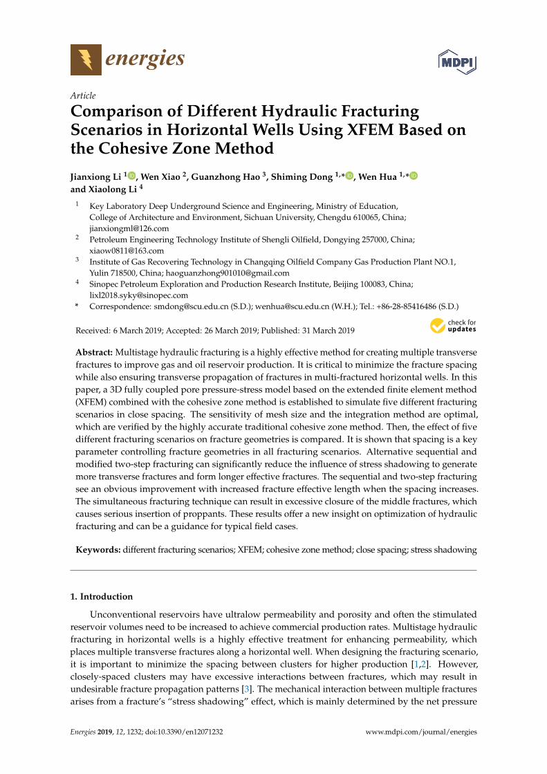
In order to avoid re-meshing during the fracture evolution, the XFEM method is introducedto model the arbitrary discontinuities in meshes, which results in a great improvement in fracturetip solutions. Compared to the traditional finite element method, the local enrichment functions areincorporated into a finite approximation function [8,9]. Therefore, the extension of new displacementfield u can be discretized into three parts based on the equilibrium equation. As shown in Figure 1,three parts of functions describe the nodes behaviors of whole elements, elements which are totallycrossed and elements with crack-tip, respectively. Further, a fully coupled pore fluid diffusion andstress analysis has been implemented by adding pore pressure node. A complete presentation of thisXFEM equation can be given in:

u = ∑I∈Sall

NuI (x)uI + ∑

I∈S f racNu

I (x)H(x)aI + ∑I∈Stip

NuI (x)

4

∑l=4

Fl(x)blI (4)

where Sall is the set of all ordinary nodes, Sfrac and Stip are the set of Heaviside enrichment nodesand the set of fracture-tip enrichment nodes, respectively. uI is node degrees of freedom in regularfinite element. aI and bl

I represent the enrichment nodal degrees of freedom for fracture and crack-tip,

Energies 2019, 12, 1232 4 of 19

respectively. NIu is the standard finite shape function of node I. H(x) is the enrichment shape jump

function. Fl is the singular displacement field around the facture tip.

Energies 2018, 11, x FOR PEER REVIEW 4 of 19

( ) 1, 01, 0

xH x

x≥

= − < (5)

where x is the signed distance function which determines the two sides of a crack. The third term is used to detail the nodes which are only cut by the crack tip. The asymptotic

crack-tip functions Fl(x) is applied to describe the displacement around the fracture tip [17]:

{ }4( , ) [ ]2 2 2 2l lF r rsin rsin sin rcos rcos cosθ θ θ θθ θ θ= ， ， ， (6)

where r and θ are the polar coordinates at the crack tip with its origin coordinate system.

Figure 1. Schematic of enrich nodes and common fluid nodes (pore-pressure nodes within a fracture).

2.3. Crack Initiation and Damage Evolution

Unlike the methods used in previous studies [18–22], the CZM method is applied because of its potential superiority in modeling softening and plastic effects of fracture tips. The constitutive behavior of the CZM is defined by the traction-separation law, which includes three steps of facture propagation: (1) loading initiation; (2) damage initiation; and (3) damage evolution.

Damage initiation occurs at the beginning of stiffness degradation of the cohesive material. The process of degradation begins when the strains and stress satisfy the critical value in the assigned criteria. In this simulation, the maximum principle is chosen:

0max

max

fσσ

=

(7)

where 0max is the maximum allowable principal stress. The symbol〈〉represents the Macaulay bracket, which is used to indicate a pure compressive stress does not initiate damage. It assumes that damage will initiate when the stress ratio f reaches the value of 1.

Once the damage initiates, a scalar variable, D, is introduced to represent the average damage in the process of fracture propagation. D evolves from 0 to 1 after damage initiation and the element stiffness has a fully degradation when D reaches a value of one. Three components of one normal stress and two shear stress are determined linearly by the damage as follows [23]:

(1 ) , 0, 0n n

nn n

D t tt

t t− ≥

= < (8)

(1 )s st D t= − (9)

(1 )t tt D t= − (10)

where nt , st and tt are the stress component in traction separation behavior without damage. Here, the index n, s, t represent the direction of normal stress and the two shear stress, respectively.

Figure 1. Schematic of enrich nodes and common fluid nodes (pore-pressure nodes within a fracture).

The second term on the right-hand of Equation (4) represents the nodes which are cut by the crackinterior. These nodes are called Heaviside enriched nodes and the function H(x) is called the jumpshape function:

H(x) =

{1, x ≥ 0

−1, x < 0(5)

where x is the signed distance function which determines the two sides of a crack.The third term is used to detail the nodes which are only cut by the crack tip. The asymptotic

crack-tip functions Fl(x) is applied to describe the displacement around the fracture tip [17]:

{Fl(r, θ)}4l = [

√rsin

θ

2,√

rsinθ

2sinθ,

√rcos

θ

2,√

rcosθ

2cosθ] (6)

where r and θ are the polar coordinates at the crack tip with its origin coordinate system.

2.3. Crack Initiation and Damage Evolution

Unlike the methods used in previous studies [18–22], the CZM method is applied because ofits potential superiority in modeling softening and plastic effects of fracture tips. The constitutivebehavior of the CZM is defined by the traction-separation law, which includes three steps of facturepropagation: (1) loading initiation; (2) damage initiation; and (3) damage evolution.

Damage initiation occurs at the beginning of stiffness degradation of the cohesive material.The process of degradation begins when the strains and stress satisfy the critical value in the assignedcriteria. In this simulation, the maximum principle is chosen:

f =

{〈σmax〉σ0

max

}(7)

where σ0max is the maximum allowable principal stress. The symbol 〈〉 represents the Macaulay bracket,

which is used to indicate a pure compressive stress does not initiate damage. It assumes that damagewill initiate when the stress ratio f reaches the value of 1.

Once the damage initiates, a scalar variable, D, is introduced to represent the average damagein the process of fracture propagation. D evolves from 0 to 1 after damage initiation and the elementstiffness has a fully degradation when D reaches a value of one. Three components of one normalstress and two shear stress are determined linearly by the damage as follows [23]:

tn =

{(1− D)tn, tn ≥ 0

tn, tn < 0(8)

Energies 2019, 12, 1232 5 of 19

ts = (1− D)ts (9)

tt = (1− D)tt (10)

where tn, ts and tt are the stress component in traction separation behavior without damage. Here,the index n, s, t represent the direction of normal stress and the two shear stress, respectively.

Many formations are considered as quasi-brittle materials, in which linear softening effect is moresuitable to simulate the process zone of fracture tip. Therefore, the variable, D, can be written linearlyas follows:

D =δ

fm(δ

maxm − δ0

m)

δmaxm (δ

fm − δ0

m)(11)

where δm is the relative effective displacement attained over the course of loading. The superscriptsmax, f and 0 represent the max relative displacement, displacement when fractures are completelydamaged, and the displacement at damage initiation.

To account for the displacement of three direction of stress, the effective separation is defined as:

δm =

√〈δn〉2 + δs

2 + δt2 (12)

where δn, δs and δt are the displacement in the direction of one normal stress and two shearstresses, respectively.

Damage evolution can be described according to the fracture energy theory, when the damageoccurs. The Benzeggagh-Kenane (BK) criterion is applied in this simulation to model the fracturepropagation. Figure 2 shows fracture evolution used by the mix-mode BK criterion. The correspondingformulas is expressed as [24]:

Gcn + (Gc

s − Gcn)

(Gs + Gt

Gn + Gs + Gt

)η

= Gc (13)

where G represents the energy release rate. Superscript c is the critical energy release rate. Thesubscripts n, s, t denote the directions of the normal stress and the two shear stresses, and η is aconstant for a corresponding material property.

Energies 2018, 11, x FOR PEER REVIEW 5 of 19

Many formations are considered as quasi-brittle materials, in which linear softening effect is more suitable to simulate the process zone of fracture tip. Therefore, the variable, D, can be written linearly as follows:

max 0

max 0

( )( )

fm m m

fm m m

D δ δ δδ δ δ

−=

− (11)

where δm is the relative effective displacement attained over the course of loading. The superscripts max, f and 0 represent the max relative displacement, displacement when fractures are completely damaged, and the displacement at damage initiation.

To account for the displacement of three direction of stress, the effective separation is defined as:

2 2 2m n + +s tδ δ δ δ= (12)

where δn, δs and δt are the displacement in the direction of one normal stress and two shear stresses, respectively.

Damage evolution can be described according to the fracture energy theory, when the damage occurs. The Benzeggagh-Kenane (BK) criterion is applied in this simulation to model the fracture propagation. Figure 2 shows fracture evolution used by the mix-mode BK criterion. The corresponding formulas is expressed as [24]:

( )c c c cs tn s n

n s t

G GG G G G

G G G

η +

+ − = + + (13)

where G represents the energy release rate. Superscript c is the critical energy release rate. The subscripts n, s, t denote the directions of the normal stress and the two shear stresses, and η is a constant for a corresponding material property.

Figure 2. Cohesive linear-softening for BK criterion.

2.4. Fluid Flow within CZM

As shown in Figure 3, both normal and tangential flow are taken into consideration in the CZM fractures. The normal flow presents the crossing behavior between fracture surface and rock deformation. The tangential flow is the fluid flow along the fracture, which can describe the gradient pressure along the fracture path. All fluid within the model are assumed to be Newtown fluid which is incompressible and governed by the lubrication equation [25].

Figure 2. Cohesive linear-softening for BK criterion.

2.4. Fluid Flow within CZM

As shown in Figure 3, both normal and tangential flow are taken into consideration in theCZM fractures. The normal flow presents the crossing behavior between fracture surface and rockdeformation. The tangential flow is the fluid flow along the fracture, which can describe the gradientpressure along the fracture path. All fluid within the model are assumed to be Newtown fluid which isincompressible and governed by the lubrication equation [25].

Energies 2019, 12, 1232 6 of 19Energies 2018, 11, x FOR PEER REVIEW 6 of 19

Figure 3. Flow of fracturing fluid within fracture.

The volume balance equation of tangential flow can be described by the following expression: 3

12 fwq p

μ= − ∇ (14)

where q is the tangential flow rate, w is the fracture width, μ is the viscosity of the fracturing fluid, and ∇pf is the gradient of pressure along the cohesive zone. This equation assumes that the injection rate is proportional to the pressure gradient and the cube of the fracture width and inversely proportional to the fracturing fluid viscosity.

The normal flow is described as:

( )( )

t t i t

b b i b

q c p pq c p p

= −= − (15)

where qt and qb are the fluid rate of permeation for the up and side surfaces, respectively; ct and cb are the leak-off coefficients of the top and bottom cohesive layers, respectively; pt and pb are the pore pressures on the top and bottom surfaces, respectively; pi is the pore pressure in the middle of the cohesive element.

Therefore, the conservation equation of fluid mass containing normal and tangential flow is summarized as [26]:

( ) Q(t) (x, y)δ∂ + ∇ + + =∂ t bw q q qt

(16)

where Q is the total volume of injection fluid.

3. Model Construction and Verification

Hydraulic fracturing using XFEM based on the CZM method is more expensive in computation, when deviation of fractures occurs. This model needs a very fine mesh in a large field of enrichment which satisfies a requirement of quick convergence of solutions [27]. All the simulations are solved by the standard solver based on the ABAQUS. In order to optimize the computing resource, we model a 3D hydraulic fracturing model using a single layer of fine element. Further, the sensitivity of mesh size and accuracy of integration method are investigated comparing with the FEM based on the CZM model, which has high accuracy in modeling hydraulic fracturing [25,28–30]. All parameters used in simulations come from the oil field of East China, as shown in Table 1.

ABAQUS presents a 3D solid element with pore pressure to model 3D hydraulic fracturing problems, which are solved by the analysis steps of geostatic and soils. Two main integration methods, including full integration (C3D8P) and reduced integration (C3D8RP) are provided to solve the problems coupling multiple factors. However, the sensitivity of mesh size and the accuracy of integration method were not verified in previous studies [3,11,13,31]. In this paper, we use a single layer whose thickness is 0.5 m. Then, the size of horizontal is refined for four types as shown in Figure 4. Further, each size of C3D8P and C3D8RP are simulated to compare with the FEM based on CZM, which has a high accuracy in modeling hydraulic fractures [15,30,32–34]. Figures 5 and 6 show that the mesh size influences the accuracy of simulation results obviously. As the refining of elements, the injection pressure and mouth opening displacement (MOD) are closer to the results of FEM based on

Figure 3. Flow of fracturing fluid within fracture.

The volume balance equation of tangential flow can be described by the following expression:

q = − w3

12µ∇p f (14)

where q is the tangential flow rate, w is the fracture width, µ is the viscosity of the fracturingfluid, and ∇pf is the gradient of pressure along the cohesive zone. This equation assumes thatthe injection rate is proportional to the pressure gradient and the cube of the fracture width andinversely proportional to the fracturing fluid viscosity.

The normal flow is described as:

qt = ct(pi − pt)

qb = cb(pi − pb)(15)

where qt and qb are the fluid rate of permeation for the up and side surfaces, respectively; ct and cbare the leak-off coefficients of the top and bottom cohesive layers, respectively; pt and pb are the porepressures on the top and bottom surfaces, respectively; pi is the pore pressure in the middle of thecohesive element.

Therefore, the conservation equation of fluid mass containing normal and tangential flow issummarized as [26]:

∂w∂t

+∇q + (qt + qb) = Q(t)δ(x, y) (16)

where Q is the total volume of injection fluid.

3. Model Construction and Verification

Hydraulic fracturing using XFEM based on the CZM method is more expensive in computation,when deviation of fractures occurs. This model needs a very fine mesh in a large field of enrichmentwhich satisfies a requirement of quick convergence of solutions [27]. All the simulations are solved bythe standard solver based on the ABAQUS. In order to optimize the computing resource, we model a3D hydraulic fracturing model using a single layer of fine element. Further, the sensitivity of meshsize and accuracy of integration method are investigated comparing with the FEM based on the CZMmodel, which has high accuracy in modeling hydraulic fracturing [25,28–30]. All parameters used insimulations come from the oil field of East China, as shown in Table 1.

ABAQUS presents a 3D solid element with pore pressure to model 3D hydraulic fracturingproblems, which are solved by the analysis steps of geostatic and soils. Two main integration methods,including full integration (C3D8P) and reduced integration (C3D8RP) are provided to solve theproblems coupling multiple factors. However, the sensitivity of mesh size and the accuracy ofintegration method were not verified in previous studies [3,11,13,31]. In this paper, we use a singlelayer whose thickness is 0.5 m. Then, the size of horizontal is refined for four types as shown inFigure 4. Further, each size of C3D8P and C3D8RP are simulated to compare with the FEM based onCZM, which has a high accuracy in modeling hydraulic fractures [15,30,32–34]. Figures 5 and 6 showthat the mesh size influences the accuracy of simulation results obviously. As the refining of elements,

Energies 2019, 12, 1232 7 of 19

the injection pressure and mouth opening displacement (MOD) are closer to the results of FEM basedon CZM. The horizontal size refines to 0.5 × 0.5 m can achieve high accuracy both using the C3D8Pand the C3D8RP. Owing to high computation speed of reduced integration, several scholars appliedthe C3D8RP in hydraulic fracturing simulations [35,36].

Table 1. Input parameters of simulations.

Parameters Values

Model dimension 300 × 150 mPerforation length 1 m

Maximum horizontal stress, σH 17 MPaMinimum horizontal stress, σh 15 MPa

Vertical stress, σv 20 MPaYoung’s modulus, E 12.94 GPa

Poisson’s ratio, υ 0.25Tensile strength, σt 1.26 MPaFracture energy, Gc 28 N/mm

Permeability, k 2.814 mDLeak-off coefficient, c 1 × 10−14 m/(pa·s)

Porosity, ϕ 0.12Fluid viscosity, µ 1 mpa·sInjection rate, Q 2 × 10−4 m3/s

Initial pore pressure, P 10 MPaFracturing time of each stage 2000 s

Injection fluid densityPower law exponent

Cluster spacingPerforation length

1000 kg/m3

2.28410, 20 m

1 m

Energies 2018, 11, x FOR PEER REVIEW 7 of 19

CZM. The horizontal size refines to 0.5 × 0.5 m can achieve high accuracy both using the C3D8P and the C3D8RP. Owing to high computation speed of reduced integration, several scholars applied the C3D8RP in hydraulic fracturing simulations [35,36].

Table 1. Input parameters of simulations.

Parameters Values

Model dimension 300 × 150 m

Perforation length 1 m

Maximum horizontal stress, σH 17 MPa

Minimum horizontal stress, σh 15 MPa

Vertical stress, σv 20 MPa

Young’s modulus, E 12.94 GPa

Poisson’s ratio, υ 0.25

Tensile strength, σt 1.26 MPa

Fracture energy, Gc 28 N/mm

Permeability, k 2.814 mD

Leak-off coefficient, c 1 × 10−14 m/(pa·s)

Porosity, φ 0.12

Fluid viscosity, μ 1 mpa·s

Injection rate, Q 2 × 10−4 m3/s

Initial pore pressure, P 10 MPa

Fracturing time of each stage 2000 s

Injection fluid density

Power law exponent

Cluster spacing

Perforation length

1000 kg/m3

2.284

10, 20 m

1 m

Figure 4. Horizontal mesh size of refinement.

Nevertheless, the injection pressure and mouth opening displacement using the C3D8P are more accurate comparing with the results from the C3D8RP, as shown in Figures 5 and 6. It indicates that the results of C3D8P have a higher accuracy than the results of C3D8RP with the requirement of mesh refinement. Further, we discovered that C3D8RP has a disadvantage in solution convergence which will result in tremendous distortion of elements, as shown in Figure 7.

Refining the mesh size can reduce the convergence failures but increasing the mesh numbers, which will increase the computational cost. Therefore, we restrict the element for C3D8P and the

Figure 4. Horizontal mesh size of refinement.

Nevertheless, the injection pressure and mouth opening displacement using the C3D8P are moreaccurate comparing with the results from the C3D8RP, as shown in Figures 5 and 6. It indicates thatthe results of C3D8P have a higher accuracy than the results of C3D8RP with the requirement of meshrefinement. Further, we discovered that C3D8RP has a disadvantage in solution convergence whichwill result in tremendous distortion of elements, as shown in Figure 7.

Refining the mesh size can reduce the convergence failures but increasing the mesh numbers,which will increase the computational cost. Therefore, we restrict the element for C3D8P and theoptimal mesh size is 0.5 × 0.5 × 0.5 m in this work. In order to keep the injection of fluid when thefracture initiates, the initial gap of enrichment is set at 2 mm.

Energies 2019, 12, 1232 8 of 19

Energies 2018, 11, x FOR PEER REVIEW 8 of 19

optimal mesh size is 0.5 × 0.5 × 0.5 m in this work. In order to keep the injection of fluid when the fracture initiates, the initial gap of enrichment is set at 2 mm.

(a) (b)

Figure 5. Variation of injection pressure and mouth opening displacement with C3D8P: (a) Variation of injection pressure; (b) Variation of mouth opening displacement.

(a) (b)

Figure 6. Variation of injection pressure and mouth opening displacement with C3D8RP: (a) Variation of injection pressure; (b) Variation of mouth opening displacement.

.

Figure 7. Distorted meshes using C3D8RP in hydraulic fracturing problems.

In order to reduce the computing cost, only one half of the model is simulated by using a symmetric model. As shown in Figure 8, the computational domain has a length of 300 m and a width of 200 m. All elements are set to be enrichment, but only 100 × 100 m domain adopts the optimal mesh size of 0.5 × 0.5 m to guarantee the accuracy of fracture propagation. In order to eliminate the effect of boundaries, the model extends far enough. Simultaneously, the domains without fracture

Figure 5. Variation of injection pressure and mouth opening displacement with C3D8P: (a) Variation ofinjection pressure; (b) Variation of mouth opening displacement.

Energies 2018, 11, x FOR PEER REVIEW 8 of 19

optimal mesh size is 0.5 × 0.5 × 0.5 m in this work. In order to keep the injection of fluid when the fracture initiates, the initial gap of enrichment is set at 2 mm.

(a) (b)

Figure 5. Variation of injection pressure and mouth opening displacement with C3D8P: (a) Variation of injection pressure; (b) Variation of mouth opening displacement.

(a) (b)

Figure 6. Variation of injection pressure and mouth opening displacement with C3D8RP: (a) Variation of injection pressure; (b) Variation of mouth opening displacement.

.

Figure 7. Distorted meshes using C3D8RP in hydraulic fracturing problems.

In order to reduce the computing cost, only one half of the model is simulated by using a symmetric model. As shown in Figure 8, the computational domain has a length of 300 m and a width of 200 m. All elements are set to be enrichment, but only 100 × 100 m domain adopts the optimal mesh size of 0.5 × 0.5 m to guarantee the accuracy of fracture propagation. In order to eliminate the effect of boundaries, the model extends far enough. Simultaneously, the domains without fracture

Figure 6. Variation of injection pressure and mouth opening displacement with C3D8RP: (a) Variationof injection pressure; (b) Variation of mouth opening displacement.

Energies 2018, 11, x FOR PEER REVIEW 8 of 19

optimal mesh size is 0.5 × 0.5 × 0.5 m in this work. In order to keep the injection of fluid when the fracture initiates, the initial gap of enrichment is set at 2 mm.

(a) (b)

Figure 5. Variation of injection pressure and mouth opening displacement with C3D8P: (a) Variation of injection pressure; (b) Variation of mouth opening displacement.

(a) (b)

Figure 6. Variation of injection pressure and mouth opening displacement with C3D8RP: (a) Variation of injection pressure; (b) Variation of mouth opening displacement.

.

Figure 7. Distorted meshes using C3D8RP in hydraulic fracturing problems.

In order to reduce the computing cost, only one half of the model is simulated by using a symmetric model. As shown in Figure 8, the computational domain has a length of 300 m and a width of 200 m. All elements are set to be enrichment, but only 100 × 100 m domain adopts the optimal mesh size of 0.5 × 0.5 m to guarantee the accuracy of fracture propagation. In order to eliminate the effect of boundaries, the model extends far enough. Simultaneously, the domains without fracture

Figure 7. Distorted meshes using C3D8RP in hydraulic fracturing problems.

In order to reduce the computing cost, only one half of the model is simulated by using asymmetric model. As shown in Figure 8, the computational domain has a length of 300 m anda width of 200 m. All elements are set to be enrichment, but only 100 × 100 m domain adoptsthe optimal mesh size of 0.5 × 0.5 m to guarantee the accuracy of fracture propagation. In orderto eliminate the effect of boundaries, the model extends far enough. Simultaneously, the domainswithout fracture propagation used the transition mesh sizes, which can reduce the computational

Energies 2019, 12, 1232 9 of 19

cost effectively. Therefore, the entire domain is discretized into 54830 elements. A zero-displacementdegree of freedom and an initial pore pressure (10 MPa) boundary are applied on the outer boundary(AB, BC, CD). Further, a symmetric boundary is set at the horizontal well (AD) and the displacementof all nodes is fixed in the thickness-direction. In order to compare the effect of different fracturingscenarios, three fracturing stages are adopted in this simulation. The numbers 1©, 2©, and 3© representthe right, middle and left fracture, respectively.

Energies 2018, 11, x FOR PEER REVIEW 9 of 19

propagation used the transition mesh sizes, which can reduce the computational cost effectively. Therefore, the entire domain is discretized into 54830 elements. A zero-displacement degree of freedom and an initial pore pressure (10 MPa) boundary are applied on the outer boundary (AB, BC, CD). Further, a symmetric boundary is set at the horizontal well (AD) and the displacement of all nodes is fixed in the thickness-direction. In order to compare the effect of different fracturing scenarios, three fracturing stages are adopted in this simulation. The numbers ① , ② , and ③ represent the right, middle and left fracture, respectively.

Figure 8. Construction of element model.

4. Results

4.1. Simultaneous Fracturing

The case of simultaneous fracturing in horizontal wells is investigated in this section, in which the fracture spacings are 10 and 20 m. The used parameters are from an oilfield in East China, as shown in Table 1. The geometries for simultaneous fracturing fractures are shown in Figure 9. The propagation of multiple fractures can influence the fracture geometries in a variety of patterns from coalescence to divergence. It indicates that the stress field changes a lot in the near region of fracture surface and fracture-tip. This phenomenon, which is induced by the propped fracture and the diffusion of pore-pressure, can result in undesirable propagation of fracture networks and reduces the efficiency of each fracturing stage.

Unlike the common assumption in previous studies that the trajectories of fractures will propagate in the direction of maximum horizontal principle stress [25,37], with simultaneous fracturing, only the middle fracture follows a direction that is perpendicular to the minimum horizontal principle stress. The side fractures tend to deviate, which is due to the stress interference induced by the middle fracture. The side fractures are suppressed to be short and wide compared with the middle fracture. Furthermore, the middle fracture can break though rapidly and negatively impact the propagation in the whole process of fracturing. Conversely, the fracture width of the middle fracture is influenced by the stress shadowing, which leads to excessive closure of the middle fracture in the near well region. The phenomenon produces an excessive pressure on the fracture surface and results in a narrow flow channel for the injection fluid. The final trajectories of fractures indicate that the side fractures deviate from the desired orthogonal paths and middle fracture suffered an excessive pressure near the wellbore. In this situation, the effectiveness of the three fractures decreases significantly.

Different results of injection pressure and MOD for the spacing at 10 and 20 m can be achieved (as shown in Figure 10a,b). From Figure 10a, we know that the injection pressure of side fractures are much higher than the middle fracture, which is caused by the stress shadowing. However, the injection pressure of the two side fractures are consistent. This indicates that the effect of side fractures can reduce the propagation pressure of the middle fracture, which is the main reason that

Figure 8. Construction of element model.

4. Results

4.1. Simultaneous Fracturing

The case of simultaneous fracturing in horizontal wells is investigated in this section, in which thefracture spacings are 10 and 20 m. The used parameters are from an oilfield in East China, as shown inTable 1. The geometries for simultaneous fracturing fractures are shown in Figure 9. The propagationof multiple fractures can influence the fracture geometries in a variety of patterns from coalescenceto divergence. It indicates that the stress field changes a lot in the near region of fracture surfaceand fracture-tip. This phenomenon, which is induced by the propped fracture and the diffusion ofpore-pressure, can result in undesirable propagation of fracture networks and reduces the efficiency ofeach fracturing stage.

Energies 2018, 11, x FOR PEER REVIEW 10 of 19

generates a deeper propagation of the middle fracture. The fracture geometries of opening and closure can influence the efficiency of hydraulic fractures. Excessive closure of fractures will result in great difficult in fluid injection and increase the possibility of proppant insertion. In this situation, the drainage of the reservoirs decreases significantly. Figure 10b presents the variation of MOD in the fracturing process. Compared with side fractures, the MOD of middle fractures decreases significantly as the two side fractures evolve. The difference is that the maximum MOD in larger spacing (20 m) is wider than with spacing = 10 m. Further, in the spacing = 10 m case, the middle fracture opens when the fractures initiate from the well, and suffers excessive suppression in the early stages of fracturing. In that situation, the mouth of the middle fracture will completely close in a short period of time. With the spacing = 20 m, even the mouth of the middle fracture will close, and the average facture width is much higher than the case of spacing = 10 m. That can be explained by the fact that an increment of spacing can reduce the stress shadowing significantly in a closely-spaced scenario. When the spacing is increased, a longstanding opening of the fracture mouth can be maintained, which is useful to the injection and placement of proppant for simultaneous fracturing.

Figure 9. Fracture geometries of simultaneous fracturing with different closely-spacing (POR is the pore pressure: Pa): (a) Fracture geometries of spacing = 10 m; (b) Fracture geometries of spacing = 20 m.

(a) (b)

Figure 10. Variation of injection pressure and mouth opening displacement with different closely-spacing simultaneous fracturing: (a) Variation of injection pressure; (b) Variation of mouth opening displacement.

4.2. Sequential and Alternative Sequential Fracturing

In this section, the sequential and alternative sequential fracturing are simulated using different close spacings of 10 and 20 m. All of parameters are listed in Table 1. Two groups of fracturing scenarios are taken into account to optimize a desirable sequential fracturing treatment in a close spacing scenario. The final fracture geometries of sequential and alternative sequential fracturing are presented in Figure 11.

Figure 9. Fracture geometries of simultaneous fracturing with different closely-spacing (POR is thepore pressure: Pa): (a) Fracture geometries of spacing = 10 m; (b) Fracture geometries of spacing = 20 m.

Unlike the common assumption in previous studies that the trajectories of fractures will propagatein the direction of maximum horizontal principle stress [25,37], with simultaneous fracturing, only themiddle fracture follows a direction that is perpendicular to the minimum horizontal principle stress.The side fractures tend to deviate, which is due to the stress interference induced by the middlefracture. The side fractures are suppressed to be short and wide compared with the middle fracture.

Energies 2019, 12, 1232 10 of 19

Furthermore, the middle fracture can break though rapidly and negatively impact the propagation inthe whole process of fracturing. Conversely, the fracture width of the middle fracture is influenced bythe stress shadowing, which leads to excessive closure of the middle fracture in the near well region.The phenomenon produces an excessive pressure on the fracture surface and results in a narrowflow channel for the injection fluid. The final trajectories of fractures indicate that the side fracturesdeviate from the desired orthogonal paths and middle fracture suffered an excessive pressure near thewellbore. In this situation, the effectiveness of the three fractures decreases significantly.

Different results of injection pressure and MOD for the spacing at 10 and 20 m can be achieved(as shown in Figure 10a,b). From Figure 10a, we know that the injection pressure of side fracturesare much higher than the middle fracture, which is caused by the stress shadowing. However, theinjection pressure of the two side fractures are consistent. This indicates that the effect of side fracturescan reduce the propagation pressure of the middle fracture, which is the main reason that generatesa deeper propagation of the middle fracture. The fracture geometries of opening and closure caninfluence the efficiency of hydraulic fractures. Excessive closure of fractures will result in great difficultin fluid injection and increase the possibility of proppant insertion. In this situation, the drainage of thereservoirs decreases significantly. Figure 10b presents the variation of MOD in the fracturing process.Compared with side fractures, the MOD of middle fractures decreases significantly as the two sidefractures evolve. The difference is that the maximum MOD in larger spacing (20 m) is wider than withspacing = 10 m. Further, in the spacing = 10 m case, the middle fracture opens when the fracturesinitiate from the well, and suffers excessive suppression in the early stages of fracturing. In thatsituation, the mouth of the middle fracture will completely close in a short period of time. With thespacing = 20 m, even the mouth of the middle fracture will close, and the average facture width ismuch higher than the case of spacing = 10 m. That can be explained by the fact that an increment ofspacing can reduce the stress shadowing significantly in a closely-spaced scenario. When the spacingis increased, a longstanding opening of the fracture mouth can be maintained, which is useful to theinjection and placement of proppant for simultaneous fracturing.

Energies 2018, 11, x FOR PEER REVIEW 10 of 19

generates a deeper propagation of the middle fracture. The fracture geometries of opening and closure can influence the efficiency of hydraulic fractures. Excessive closure of fractures will result in great difficult in fluid injection and increase the possibility of proppant insertion. In this situation, the drainage of the reservoirs decreases significantly. Figure 10b presents the variation of MOD in the fracturing process. Compared with side fractures, the MOD of middle fractures decreases significantly as the two side fractures evolve. The difference is that the maximum MOD in larger spacing (20 m) is wider than with spacing = 10 m. Further, in the spacing = 10 m case, the middle fracture opens when the fractures initiate from the well, and suffers excessive suppression in the early stages of fracturing. In that situation, the mouth of the middle fracture will completely close in a short period of time. With the spacing = 20 m, even the mouth of the middle fracture will close, and the average facture width is much higher than the case of spacing = 10 m. That can be explained by the fact that an increment of spacing can reduce the stress shadowing significantly in a closely-spaced scenario. When the spacing is increased, a longstanding opening of the fracture mouth can be maintained, which is useful to the injection and placement of proppant for simultaneous fracturing.

Figure 9. Fracture geometries of simultaneous fracturing with different closely-spacing (POR is the pore pressure: Pa): (a) Fracture geometries of spacing = 10 m; (b) Fracture geometries of spacing = 20 m.

(a) (b)

Figure 10. Variation of injection pressure and mouth opening displacement with different closely-spacing simultaneous fracturing: (a) Variation of injection pressure; (b) Variation of mouth opening displacement.

4.2. Sequential and Alternative Sequential Fracturing

In this section, the sequential and alternative sequential fracturing are simulated using different close spacings of 10 and 20 m. All of parameters are listed in Table 1. Two groups of fracturing scenarios are taken into account to optimize a desirable sequential fracturing treatment in a close spacing scenario. The final fracture geometries of sequential and alternative sequential fracturing are presented in Figure 11.

Figure 10. Variation of injection pressure and mouth opening displacement with differentclosely-spacing simultaneous fracturing: (a) Variation of injection pressure; (b) Variation of mouthopening displacement.

4.2. Sequential and Alternative Sequential Fracturing

In this section, the sequential and alternative sequential fracturing are simulated using differentclose spacings of 10 and 20 m. All of parameters are listed in Table 1. Two groups of fracturingscenarios are taken into account to optimize a desirable sequential fracturing treatment in a close

Energies 2019, 12, 1232 11 of 19

spacing scenario. The final fracture geometries of sequential and alternative sequential fracturing arepresented in Figure 11.

Energies 2018, 11, x FOR PEER REVIEW 11 of 19

In case 1 (Figure 11a), the sequential fracturing is applied in the situation of spacing = 10 m, whose fracturing sequence is ①-②-③ (right fracture–middle fracture–left fracture). In this situation, only the right fracture (first fracture) propagates along an orthogonal path and extends deepest compared with the subsequent fractured fractures. The middle fracture (second fracture) and left fractures (third fracture) deviate from the desirable direction significantly, and present obvious coalescence with the right fracture. Moreover, the middle fracture propagates deeper than the left fracture, which can be explained by the fact that the left fracture has suffered stronger influence from the prior fractured right and middle fracture. However, the middle fracture is only influenced by the right fracture. Owing to stress shadowing in the third fracturing stage, the right and middle fractures come to be closed near the wellbore. Simultaneously, the width of the right fracture decreases the most and tends to close completely in the near well region. The fracture geometries of case 3 (Figure 11c) are much different in case 1. In case 3, the alternative fracturing uses a scenario of spacing = 10 m, whose fracturing sequence is ① - ③ -② (right fracture–left fracture–middle fracture). The alternative sequence can enhance the propagation of the left fracture (second fracture), but suppresses the propagation of the middle fracture (third fracture). Further, less deviation of fractures can be observed in the alternative sequential fracturing comparing with the sequential fracturing. This denotes that fracturing sequence can easily change the fracture geometries in a close spacing situation. In the case 2 (Figure 11b) and case 4 (Figure 11d), the geometries change a lot both in sequential and alternative sequential fracturing, when the spacing increases from 10 to 20 m. It denotes that spacing is a key parameter in controlling the fracture geometries. However, the left fracture propagates longer and the middle fracture presents more curvature, when the alternative sequential fracturing is applied. This demonstrates that the alternative sequence can enhance the interference on the middle fracture similar to the simultaneous fracturing, but alleviates the suppression on the left fracture.

Figure 11. Fracture geometries of sequential and alternative sequential fracturing with different closely-spacing (POR is the pore pressure: Pa): (a) Fracture geometries of sequential fracturing with spacing = 10 m; (b) Fracture geometries of sequential fracturing with spacing = 20 m; (c) Fracture geometries of alternative sequential fracturing with spacing = 10 m; (d) Fracture geometries of alternative sequential fracturing with spacing = 20 m.

In order to investigate the efficiency of different fracturing scenarios, the variation of injection pressure and MOD with sequential and alternative sequential fracturing are shown in Figure 12. As shown in Figure 12a,c, all stages are fracturing continuously without a flow back of injection fluid, which can simulate the propping of proppants. Therefore, the injection pressure of each fracture

Figure 11. Fracture geometries of sequential and alternative sequential fracturing with differentclosely-spacing (POR is the pore pressure: Pa): (a) Fracture geometries of sequential fracturing withspacing = 10 m; (b) Fracture geometries of sequential fracturing with spacing = 20 m; (c) Fracturegeometries of alternative sequential fracturing with spacing = 10 m; (d) Fracture geometries ofalternative sequential fracturing with spacing = 20 m.

In case 1 (Figure 11a), the sequential fracturing is applied in the situation of spacing = 10 m, whosefracturing sequence is 1©- 2©- 3© (right fracture–middle fracture–left fracture). In this situation, onlythe right fracture (first fracture) propagates along an orthogonal path and extends deepest comparedwith the subsequent fractured fractures. The middle fracture (second fracture) and left fractures (thirdfracture) deviate from the desirable direction significantly, and present obvious coalescence with theright fracture. Moreover, the middle fracture propagates deeper than the left fracture, which can beexplained by the fact that the left fracture has suffered stronger influence from the prior fractured rightand middle fracture. However, the middle fracture is only influenced by the right fracture. Owingto stress shadowing in the third fracturing stage, the right and middle fractures come to be closednear the wellbore. Simultaneously, the width of the right fracture decreases the most and tends toclose completely in the near well region. The fracture geometries of case 3 (Figure 11c) are muchdifferent in case 1. In case 3, the alternative fracturing uses a scenario of spacing = 10 m, whosefracturing sequence is 1©- 3©- 2© (right fracture–left fracture–middle fracture). The alternative sequencecan enhance the propagation of the left fracture (second fracture), but suppresses the propagation of themiddle fracture (third fracture). Further, less deviation of fractures can be observed in the alternativesequential fracturing comparing with the sequential fracturing. This denotes that fracturing sequencecan easily change the fracture geometries in a close spacing situation. In the case 2 (Figure 11b) andcase 4 (Figure 11d), the geometries change a lot both in sequential and alternative sequential fracturing,when the spacing increases from 10 to 20 m. It denotes that spacing is a key parameter in controllingthe fracture geometries. However, the left fracture propagates longer and the middle fracture presentsmore curvature, when the alternative sequential fracturing is applied. This demonstrates that thealternative sequence can enhance the interference on the middle fracture similar to the simultaneousfracturing, but alleviates the suppression on the left fracture.

Energies 2019, 12, 1232 12 of 19

In order to investigate the efficiency of different fracturing scenarios, the variation of injectionpressure and MOD with sequential and alternative sequential fracturing are shown in Figure 12.As shown in Figure 12a,c, all stages are fracturing continuously without a flow back of injection fluid,which can simulate the propping of proppants. Therefore, the injection pressure of each fractureremains constant, when the fracturing stage is completed (injection rate = 0 m3/s). When the initialfracture damages completely, the injection pressure of all cases decreases to a stable value whichcan guarantee the propagation of fractures. It is obvious that the latter fracturing stage has a higherinjection pressure than previous fracturing stages, whether use the sequential or alternative sequentialfracturing scenarios. Compared with the sequential fracturing, the second fractures in alternativefracturing have a lower injection pressure (close to 19.3 MPa), which is almost identical to the injectionpressure of the first fractures (close to 18.8 MPa). However, the injection pressure of second fractures(close to 19.6 MPa) in sequential fracturing are closer to that of the third fractures (close to 20.2 MPa).Notably, the injection pressure of each fracturing stage is consistent when the spacing increases from10 to 20 m. It demonstrates that the spacing hardly influences the injection pressure in a close spacingscenario, when using the same fracturing scenario.

Energies 2018, 11, x FOR PEER REVIEW 12 of 19

remains constant, when the fracturing stage is completed (injection rate = 0 m3/s). When the initial fracture damages completely, the injection pressure of all cases decreases to a stable value which can guarantee the propagation of fractures. It is obvious that the latter fracturing stage has a higher injection pressure than previous fracturing stages, whether use the sequential or alternative sequential fracturing scenarios. Compared with the sequential fracturing, the second fractures in alternative fracturing have a lower injection pressure (close to 19.3 MPa), which is almost identical to the injection pressure of the first fractures (close to 18.8 MPa). However, the injection pressure of second fractures (close to 19.6 MPa) in sequential fracturing are closer to that of the third fractures (close to 20.2 MPa). Notably, the injection pressure of each fracturing stage is consistent when the spacing increases from 10 to 20 m. It demonstrates that the spacing hardly influences the injection pressure in a close spacing scenario, when using the same fracturing scenario.

Figure 12b,d show the MOD with sequential and alternative sequential fracturing. Without the influence of stress shadowing, the MOD curves show no difference between two fracturing scenarios in the first fracturing stage. The MOD of sequential fracturing fracture decreases faster than the alternative sequential fracturing in the latter fracturing stage. In this process, the MOD in the case of spacing = 20 m is always larger than the case of spacing = 10 m, which is due to the stronger influence of fracture-induced stress with shorter spacing. In the second and third fracturing stage, the MOD of first fractures decreases due to strong stress shadowing. In the situation of spacing = 10 m, the fracture mouth closes completely in the second fracturing stage (fracturing time of closure = 3850 s), which should be avoided for serious insertion of proppants, while in the situation of spacing =20 m, the first fracture remains open even all three fracturing stages are completed. The second fractured fractures experience a propagation pattern that is similar to the first fracture. However, a higher value of MOD can be achieved in the second fracturing stage, which is mainly caused by a higher value of the injection pressure. In this situation, the second fracture of sequential fracturing also has a larger MOD comparing with the alternative sequential fracturing. In the third fracturing stage of sequential fracturing, the second fracture in situation of spacing = 10 closes obviously. While in the situation of spacing = 20 m, the MOD of second fracture decreases in a short time and remains at a constant (close to 14.6 mm) value during the fracturing process. This may ensure a high efficient hydraulic fracture and reduces the possibility of proppant insertion. For the third fractures, all cases have a sharp increase of MOD except the case of sequential fracturing at spacing = 20 m. That can be explain that less stress interference leads to less consumption of injection rates in broadening the fracture. In that case, deeper propagation can be achieved for increasing the reservoir production.

(a) (b)

Energies 2018, 11, x FOR PEER REVIEW 13 of 19

Figure 12. Cont.

(c) (d) Figure 12. Variation of injection pressure and mouth opening displacement with different closely-spacing sequential and alternative sequential fracturing: (a) Variation of injection pressure with sequential fracturing; (b) Variation of mouth opening displacement with sequential fracturing; (c) Variation of injection pressure with alternative sequential fracturing; (d) Variation of mouth opening displacement with alternative sequential fracturing.

4.3. Two-step Fracturing and Modified Two-step Fracturing

In order to enhance production in the reservoirs, it is important to minimize the fracture spacing while ensures the propagation of transverse fractures. In this section, the two-step and modified two-step fracturing are simulated to investigate the effect on the facture geometries, as shown in Figure 13. In our simulation, two closely-spacing of 10, 20 m are used in the different two-step scenarios.

In case 1 (Figure 13a), the spacing equals to 10 m and the fracturing sequence is ①-②② (middle fracture – left and right fracture), which is called two-step fracturing. In this situation, the middle fracture (first fracture) initiates and propagates along a desirable orthogonal path. Then the side fractures are influenced by the middle fracture and tend to deviate seriously. As the fracturing progresses, the fracture tip of the side fractures reorient to the surface of the middle fracture, which will result in a more curved and shorter propagation path. Further, the fracture-induced stress of side fractures can conversely lead to excessive pressure on the surface of the middle fracture. Therefore, the middle fracture suffers obvious closure near the propagation path of the two side fractures. The similar propagation patterns can be observed in the condition of spacing = 20 m, but less deviation occurs in the larger spacing, as shown in Figure 13b.

In case 3 (Figure 13c), the modified two-step fracturing is applied in the condition of spacing = 10 m. The fracturing sequence is ①①-② (right and left fracture – middle fracture). In this situation, the left and right fracture initiate and deviate from each other in the first fracturing stage. The lengths of the two side fractures are bigger than the length of the fracture in two-step fracturing and even an obvious stress interference effect can be observed. For the second fractured middle fracture, the growth is suppressed significantly in the whole process and the length is much smaller than the two side fractures. An undesirable effect of middle fracture is that the behavior of coalescence that leads an excessive closure for the right fracture, which will reduce the efficiency of the right fracture due to proppant insertion. With increasing spacing (spacing = 20 m (Figure 13d)), the less effect of stress interference realizes an average propagation of multiple fractures, especially for the middle fracture whose length is longer than in the condition of spacing = 10 m.

Figure 12. Variation of injection pressure and mouth opening displacement with different closely-spacingsequential and alternative sequential fracturing: (a) Variation of injection pressure with sequentialfracturing; (b) Variation of mouth opening displacement with sequential fracturing; (c) Variation ofinjection pressure with alternative sequential fracturing; (d) Variation of mouth opening displacementwith alternative sequential fracturing.

Energies 2019, 12, 1232 13 of 19

Figure 12b,d show the MOD with sequential and alternative sequential fracturing. Without theinfluence of stress shadowing, the MOD curves show no difference between two fracturing scenariosin the first fracturing stage. The MOD of sequential fracturing fracture decreases faster than thealternative sequential fracturing in the latter fracturing stage. In this process, the MOD in the case ofspacing = 20 m is always larger than the case of spacing = 10 m, which is due to the stronger influenceof fracture-induced stress with shorter spacing. In the second and third fracturing stage, the MODof first fractures decreases due to strong stress shadowing. In the situation of spacing = 10 m, thefracture mouth closes completely in the second fracturing stage (fracturing time of closure = 3850 s),which should be avoided for serious insertion of proppants, while in the situation of spacing = 20 m,the first fracture remains open even all three fracturing stages are completed. The second fracturedfractures experience a propagation pattern that is similar to the first fracture. However, a higher valueof MOD can be achieved in the second fracturing stage, which is mainly caused by a higher value ofthe injection pressure. In this situation, the second fracture of sequential fracturing also has a largerMOD comparing with the alternative sequential fracturing. In the third fracturing stage of sequentialfracturing, the second fracture in situation of spacing = 10 closes obviously. While in the situationof spacing = 20 m, the MOD of second fracture decreases in a short time and remains at a constant(close to 14.6 mm) value during the fracturing process. This may ensure a high efficient hydraulicfracture and reduces the possibility of proppant insertion. For the third fractures, all cases have a sharpincrease of MOD except the case of sequential fracturing at spacing = 20 m. That can be explain thatless stress interference leads to less consumption of injection rates in broadening the fracture. In thatcase, deeper propagation can be achieved for increasing the reservoir production.

4.3. Two-step Fracturing and Modified Two-step Fracturing

In order to enhance production in the reservoirs, it is important to minimize the fracture spacingwhile ensures the propagation of transverse fractures. In this section, the two-step and modifiedtwo-step fracturing are simulated to investigate the effect on the facture geometries, as shown inFigure 13. In our simulation, two closely-spacing of 10, 20 m are used in the different two-step scenarios.Energies 2018, 11, x FOR PEER REVIEW 14 of 19

Figure 13. Fracture geometries of two-step and modified two-step fracturing with different closely-spacing (POR is the pore pressure: Pa): (a) Fracture geometries of two-step fracturing with spacing = 10 m; (b) Fracture geometries of two-step fracturing with spacing = 20 m; (c) Fracture geometries of modified two-step fracturing with spacing = 10 m; (d) Fracture geometries of modified two-step fracturing with spacing = 20 m.

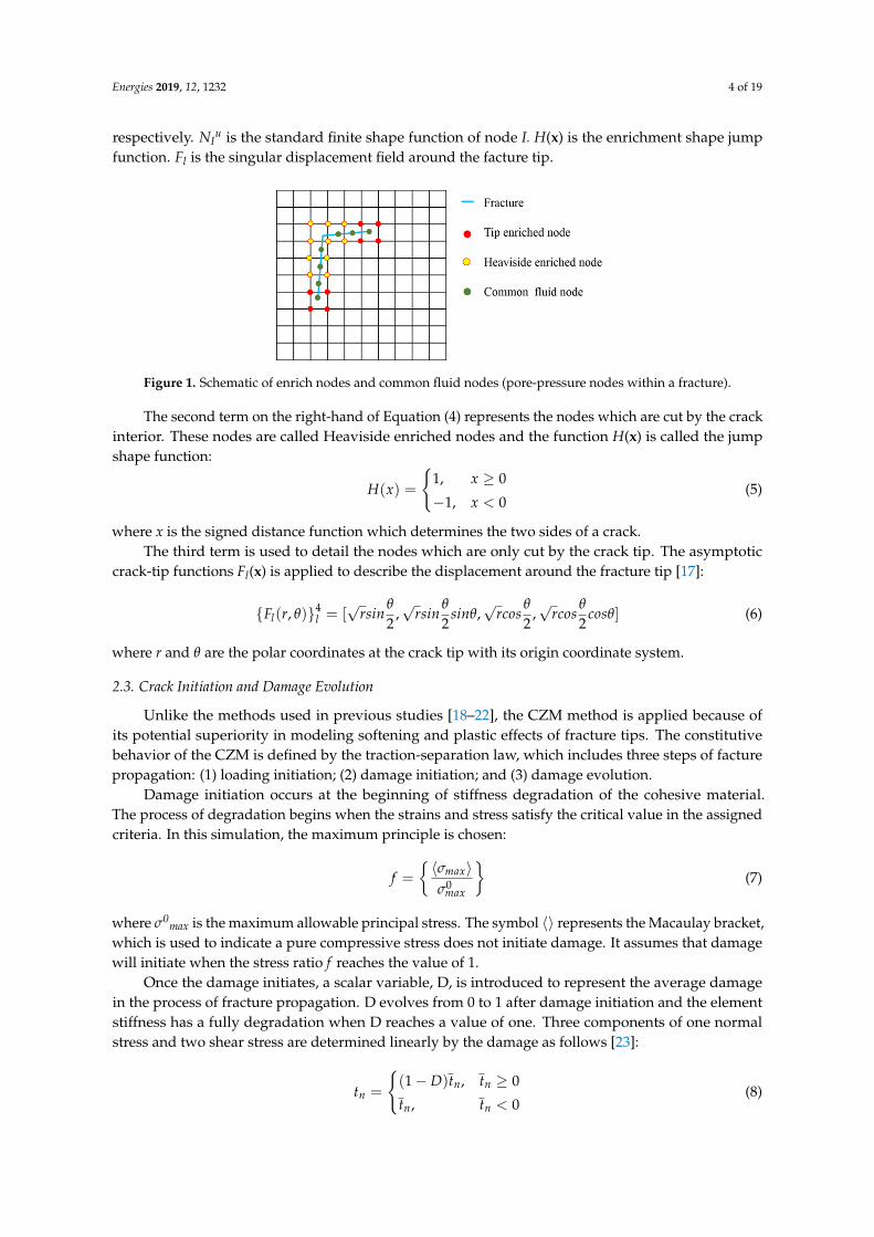
The variation of injection pressure and MOD are calculated in this simulation as shown in Figure 14. In the first fracturing stage, the injection pressure decreases to a stable value (close to 19.4 MPa) after the initiation of first fractures and few differences are observed when two different fracturing scenarios are used (Figure 14a,c). In the second fracturing stage, the second fractures have a higher injection pressure during the whole process compared with the first fracturing stage. For two-step fracturing, the injection pressure of second fractures is bigger than it is in modified two-step fracturing. Using different spacing = 10, 20 m, the injection pressure changes less. The two fracturing scenarios have different behaviors on the effect of MOD. When the middle fractures are first fractured (Figure 14b), the MOD of the middle fracture increases in the first fracturing stage, while it decreases to the value of the initial opening gap (2 mm) in the latter fracturing stage. During the process of decrease, the MOD in the condition of spacing = 10 m is smaller and reduces quicker than when spacing = 20 m. However, the MOD of the first fractures using modified two-step fracturing are quite different from the results of two-step fracturing, as shown in Figure 14d.

(a) (b)

Figure 13. Fracture geometries of two-step and modified two-step fracturing with differentclosely-spacing (POR is the pore pressure: Pa): (a) Fracture geometries of two-step fracturing withspacing = 10 m; (b) Fracture geometries of two-step fracturing with spacing = 20 m; (c) Fracturegeometries of modified two-step fracturing with spacing = 10 m; (d) Fracture geometries of modifiedtwo-step fracturing with spacing = 20 m.

Energies 2019, 12, 1232 14 of 19

In case 1 (Figure 13a), the spacing equals to 10 m and the fracturing sequence is 1©- 2© 2© (middlefracture–left and right fracture), which is called two-step fracturing. In this situation, the middlefracture (first fracture) initiates and propagates along a desirable orthogonal path. Then the sidefractures are influenced by the middle fracture and tend to deviate seriously. As the fracturingprogresses, the fracture tip of the side fractures reorient to the surface of the middle fracture, whichwill result in a more curved and shorter propagation path. Further, the fracture-induced stress of sidefractures can conversely lead to excessive pressure on the surface of the middle fracture. Therefore, themiddle fracture suffers obvious closure near the propagation path of the two side fractures. The similarpropagation patterns can be observed in the condition of spacing = 20 m, but less deviation occurs inthe larger spacing, as shown in Figure 13b.

In case 3 (Figure 13c), the modified two-step fracturing is applied in the condition of spacing = 10 m.The fracturing sequence is 1© 1©- 2© (right and left fracture–middle fracture). In this situation, the leftand right fracture initiate and deviate from each other in the first fracturing stage. The lengths ofthe two side fractures are bigger than the length of the fracture in two-step fracturing and even anobvious stress interference effect can be observed. For the second fractured middle fracture, the growthis suppressed significantly in the whole process and the length is much smaller than the two sidefractures. An undesirable effect of middle fracture is that the behavior of coalescence that leads anexcessive closure for the right fracture, which will reduce the efficiency of the right fracture due toproppant insertion. With increasing spacing (spacing = 20 m (Figure 13d)), the less effect of stressinterference realizes an average propagation of multiple fractures, especially for the middle fracturewhose length is longer than in the condition of spacing = 10 m.

The variation of injection pressure and MOD are calculated in this simulation as shown inFigure 14. In the first fracturing stage, the injection pressure decreases to a stable value (close to19.4 MPa) after the initiation of first fractures and few differences are observed when two differentfracturing scenarios are used (Figure 14a,c). In the second fracturing stage, the second fractureshave a higher injection pressure during the whole process compared with the first fracturing stage.For two-step fracturing, the injection pressure of second fractures is bigger than it is in modifiedtwo-step fracturing. Using different spacing = 10, 20 m, the injection pressure changes less. The twofracturing scenarios have different behaviors on the effect of MOD. When the middle fractures are firstfractured (Figure 14b), the MOD of the middle fracture increases in the first fracturing stage, whileit decreases to the value of the initial opening gap (2 mm) in the latter fracturing stage. During theprocess of decrease, the MOD in the condition of spacing = 10 m is smaller and reduces quicker thanwhen spacing = 20 m. However, the MOD of the first fractures using modified two-step fracturing arequite different from the results of two-step fracturing, as shown in Figure 14d.

Energies 2018, 11, x FOR PEER REVIEW 14 of 19

Figure 13. Fracture geometries of two-step and modified two-step fracturing with different closely-spacing (POR is the pore pressure: Pa): (a) Fracture geometries of two-step fracturing with spacing = 10 m; (b) Fracture geometries of two-step fracturing with spacing = 20 m; (c) Fracture geometries of modified two-step fracturing with spacing = 10 m; (d) Fracture geometries of modified two-step fracturing with spacing = 20 m.

The variation of injection pressure and MOD are calculated in this simulation as shown in Figure 14. In the first fracturing stage, the injection pressure decreases to a stable value (close to 19.4 MPa) after the initiation of first fractures and few differences are observed when two different fracturing scenarios are used (Figure 14a,c). In the second fracturing stage, the second fractures have a higher injection pressure during the whole process compared with the first fracturing stage. For two-step fracturing, the injection pressure of second fractures is bigger than it is in modified two-step fracturing. Using different spacing = 10, 20 m, the injection pressure changes less. The two fracturing scenarios have different behaviors on the effect of MOD. When the middle fractures are first fractured (Figure 14b), the MOD of the middle fracture increases in the first fracturing stage, while it decreases to the value of the initial opening gap (2 mm) in the latter fracturing stage. During the process of decrease, the MOD in the condition of spacing = 10 m is smaller and reduces quicker than when spacing = 20 m. However, the MOD of the first fractures using modified two-step fracturing are quite different from the results of two-step fracturing, as shown in Figure 14d.

(a) (b)

Figure 14. Cont.

Energies 2019, 12, 1232 15 of 19Energies 2018, 11, x FOR PEER REVIEW 15 of 19

Figure 14. Cont.

(c) (d)

Figure 14. Variation of injection pressure and mouth opening displacement with different closely-spacing two-step and modified two-step fracturing; (a) Variation of injection pressure with two-step fracturing; (b) Variation of mouth opening displacement with two-step fracturing; (c) Variation of injection pressure with modified two-step fracturing; (d) Variation of mouth opening displacement with modified two-step fracturing.

Both right and left fractures have different performance on MOD whether the spacing is 10 or 20 m. In the first fracturing stage of spacing = 10 m, we calculate that the MOD of left fracture experiences a rapidly increase and achieves a biggest value (16.18 mm), while the MOD of right fracture increases slowly and even starts to decrease in the later period of the first fracturing stage. That can be explained by the fact that the middle fracture has an obvious coalescence into the right fracture, which results in excessive suppression on the fracture wall of the right fracture. This phenomenon is observed in Figure 13c and should be avoided. In the second fracturing stage, all cases of MOD increase similarly and are consistent with each other.

5. Discussion

When considering the five fracturing scenarios together, the geometries of multiple fractures can be significantly influenced by different fracturing scenarios in a close spacing scenario. Different propagation patterns from fracture coalescence to divergence are formed because of fracture-induced stress shadowing. Using the simultaneous fracturing in close spacing, the side fractures experience obvious coalescence and outward deviation, while the middle fracture forms a transverse fracture. This phenomenon is similar to the results from Haddad et al. [10]. Further, the middle fracture can break though and gets away from the influenced region of side fractures rapidly. Therefore, the middle fracture is much longer than the side fractures. The side fractures are suppressed seriously by the middle fracture and tend to form more curved fractures, which are shorter and wider. Inversely, the excessive opening of side fractures will result in excessive closure of the middle fracture along the propagation paths of the side fractures.

Compared with sequential fracturing, the alternative sequential fracturing can reduce the interference of stress shadowing and form more transverse fractures. Increasing the spacing will alleviate the influence both in sequential and alternative sequential fracturing, which is consistent with the conclusions stated by Wang et al. [1]. Using an alternative fracturing, the optimal spacing can be reduced again. In this paper, we found that the later fracturing stage has a higher injection pressure compared with earlier fracturing stage, and the latter fractured fractures experience more serious suppression in the fracture growth. This indicates that increasing the number of fracturing stages is harmful to increasing the volume of the fracture network when close spacing is used. Further, the latter fractured fractures will result in excessive closure of previous fractures, which

Figure 14. Variation of injection pressure and mouth opening displacement with differentclosely-spacing two-step and modified two-step fracturing; (a) Variation of injection pressure withtwo-step fracturing; (b) Variation of mouth opening displacement with two-step fracturing; (c) Variationof injection pressure with modified two-step fracturing; (d) Variation of mouth opening displacementwith modified two-step fracturing.

Both right and left fractures have different performance on MOD whether the spacing is 10 or 20 m.In the first fracturing stage of spacing = 10 m, we calculate that the MOD of left fracture experiences arapidly increase and achieves a biggest value (16.18 mm), while the MOD of right fracture increasesslowly and even starts to decrease in the later period of the first fracturing stage. That can be explainedby the fact that the middle fracture has an obvious coalescence into the right fracture, which resultsin excessive suppression on the fracture wall of the right fracture. This phenomenon is observed inFigure 13c and should be avoided. In the second fracturing stage, all cases of MOD increase similarlyand are consistent with each other.

5. Discussion

When considering the five fracturing scenarios together, the geometries of multiple fracturescan be significantly influenced by different fracturing scenarios in a close spacing scenario. Differentpropagation patterns from fracture coalescence to divergence are formed because of fracture-inducedstress shadowing. Using the simultaneous fracturing in close spacing, the side fractures experienceobvious coalescence and outward deviation, while the middle fracture forms a transverse fracture.This phenomenon is similar to the results from Haddad et al. [10]. Further, the middle fracture canbreak though and gets away from the influenced region of side fractures rapidly. Therefore, the middlefracture is much longer than the side fractures. The side fractures are suppressed seriously by themiddle fracture and tend to form more curved fractures, which are shorter and wider. Inversely,the excessive opening of side fractures will result in excessive closure of the middle fracture along thepropagation paths of the side fractures.

Compared with sequential fracturing, the alternative sequential fracturing can reduce theinterference of stress shadowing and form more transverse fractures. Increasing the spacing willalleviate the influence both in sequential and alternative sequential fracturing, which is consistentwith the conclusions stated by Wang et al. [1]. Using an alternative fracturing, the optimal spacingcan be reduced again. In this paper, we found that the later fracturing stage has a higher injectionpressure compared with earlier fracturing stage, and the latter fractured fractures experience moreserious suppression in the fracture growth. This indicates that increasing the number of fracturingstages is harmful to increasing the volume of the fracture network when close spacing is used. Further,the latter fractured fractures will result in excessive closure of previous fractures, which leads to

Energies 2019, 12, 1232 16 of 19

a serious insertion of proppant. This undesirable effect can be alleviated by using the alternativefracturing treatment.

Kumar et al. [3] found that the two-step fracturing can be used in a relatively closely spacedscenario and enhance the reservoir permeability efficiently. The same conclusion was reached inour work. Using the two-step and modified two-step fracturing, the geometries of fractures can beobviously changed. In two-step fracturing, the middle fracture propagates along a desirable orthogonalpath to form transverse fracture. While the side fractures have an obvious behavior of coalescenceto the middle fracture, especially under the condition of close spacing = 10 m. However, the sidefractures can propagate more transversely and longer when the modified two-step fracturing is used,but the middle fracture can be suppressed because of the two side fractures. In conclusion, the secondfractured fractures always suffers an influence of the first fractured fractures. The modified fracturingproduces an obvious improvement of the flow efficiency of fractures in a close spacing scenario.

In order to better understand the effect of different fracturing scenarios, the effective fracturelength is provided in Figure 15. We consider a propagation depth of fractures as the effective fracturelength. When the spacing increases, the effective fracture length increases in all fracturing scenarios.This indicates that spacing is a key factor in controlling the fracture geometries, even with closespacing. When the close spacing = 10 m, alternative sequential and modified two-step fracturing havean obvious advantage compared with other fracture scenarios, whose effective fracture length canreach 156 and 155 m, respectively. However, when the spacing increases to 20 m, the sequential andtwo-step fracturing show a large increase in effective fracture length, while the effective fracture lengthof modified two-step and alternative fracturing change less in this situation. Therefore, in a closespacing scenario (10 m), the alternative and modified fracturing scenario are recommended to generatemore efficient fractures. However, the modified two-step can achieve less improvement of fracturelength when the spacing increases to 20 m. This means that increasing spacing seems meaninglesswhen the modified two-step fracturing is applied in a close spacing environment.

Energies 2018, 11, x FOR PEER REVIEW 16 of 19

leads to a serious insertion of proppant. This undesirable effect can be alleviated by using the alternative fracturing treatment.

Kumar et al. [3] found that the two-step fracturing can be used in a relatively closely spaced scenario and enhance the reservoir permeability efficiently. The same conclusion was reached in our work. Using the two-step and modified two-step fracturing, the geometries of fractures can be obviously changed. In two-step fracturing, the middle fracture propagates along a desirable orthogonal path to form transverse fracture. While the side fractures have an obvious behavior of coalescence to the middle fracture, especially under the condition of close spacing = 10 m. However, the side fractures can propagate more transversely and longer when the modified two-step fracturing is used, but the middle fracture can be suppressed because of the two side fractures. In conclusion, the second fractured fractures always suffers an influence of the first fractured fractures. The modified fracturing produces an obvious improvement of the flow efficiency of fractures in a close spacing scenario.

In order to better understand the effect of different fracturing scenarios, the effective fracture length is provided in Figure 15. We consider a propagation depth of fractures as the effective fracture length. When the spacing increases, the effective fracture length increases in all fracturing scenarios. This indicates that spacing is a key factor in controlling the fracture geometries, even with close spacing. When the close spacing = 10 m, alternative sequential and modified two-step fracturing have an obvious advantage compared with other fracture scenarios, whose effective fracture length can reach 156 and 155 m, respectively. However, when the spacing increases to 20 m, the sequential and two-step fracturing show a large increase in effective fracture length, while the effective fracture length of modified two-step and alternative fracturing change less in this situation. Therefore, in a close spacing scenario (10 m), the alternative and modified fracturing scenario are recommended to generate more efficient fractures. However, the modified two-step can achieve less improvement of fracture length when the spacing increases to 20 m. This means that increasing spacing seems meaningless when the modified two-step fracturing is applied in a close spacing environment.

Figure 15. Variation of effective fracture length with different closely-spacing fracturing scenarios.

6. Conclusions

Multistage hydraulic fracturing in horizontal wells is developed based on a 3D-XFEM, which couples the pore pressure-stress combining the cohesive zone method. Five different fracturing scenarios, including simultaneous, sequential, alternative sequential, two-step and modified two-step fracturing are simulated to investigate the impact of fracture-induced interference on fracture geometries in close spacing scenarios. The results of the five different scenarios are compared. Based on the simulations, the following conclusions can be reached:

(1) Fracture spacing is a key parameter in controlling the geometries of multiple fractures. Narrower spacing results in stronger interference of stress shadowing, which leads to a shorter

Figure 15. Variation of effective fracture length with different closely-spacing fracturing scenarios.

6. Conclusions

Multistage hydraulic fracturing in horizontal wells is developed based on a 3D-XFEM, whichcouples the pore pressure-stress combining the cohesive zone method. Five different fracturingscenarios, including simultaneous, sequential, alternative sequential, two-step and modified two-stepfracturing are simulated to investigate the impact of fracture-induced interference on fracturegeometries in close spacing scenarios. The results of the five different scenarios are compared. Basedon the simulations, the following conclusions can be reached:

(1) Fracture spacing is a key parameter in controlling the geometries of multiple fractures.Narrower spacing results in stronger interference of stress shadowing, which leads to a shorter fracture

Energies 2019, 12, 1232 17 of 19

length and wider fracture width for latter fractured fractures. The latter fractured fractures also havean undesirable effect on excessive closure of previously fractured fractures.

(2) The stress shadowing in the propagation domain is redistributed when different scenarios areused. In a close spacing scenario (10 m), alternative sequential and modified two-step fracturing cansignificantly reduce the influence of stress shadowing to generate more transverse fractures and longereffective fracture lengths.

(3) The sequential and two-step fracturing have an obvious improvement in increasing fractureeffective length when the spacing increases. Thus, more transverse and less closure of fractures willoccur by increasing the spacing, when the two fracturing scenarios are used.

(4) The simultaneous fracturing technique can result in an excessive closure of the middle fracture,which causes serious insertion of proppants. In the later fracturing process, the injection of fluid willbe difficult. The larger spacing should be optimal to reduce the influence on this situation.

The numerical model presented in this paper can be a guidance in optimizing the fracturing scenariosin closely-spacing horizontal wells.

Author Contributions: Conceptualization, J.L. and S.D.; Methodology, J.L.; Software, S.D.; Validation, W.X. andX.L.; Formal Analysis, G.H.; Investigation, J.L.; Resources, W.H.; Data Curation, W.H.; Writing-Original DraftPreparation, J.L.; Writing-Review & Editing, J.L.; Visualization, J.L.; Supervision, S.D.; Project Administration,S.D.; Funding Acquisition, S.D. and W.H.

Funding: This work was supported by the Sichuan Science and Technology Program (Project No.2018JY0024),and National Natural Science Foundation of China (Project No.11872042), the Sichuan Science and TechnologyProgram (2019YJ0156).

Conflicts of Interest: The authors declare no conflict of interest.

References

1. Wang, X.; Liu, C.; Wang, H.; Liu, H.; Wu, H. Comparison of consecutive and alternate hydraulic fracturingin horizontal wells using XFEM-based cohesive zone method. J. Pet. Sci. Eng. 2016, 143, 14–25. [CrossRef]

2. Craig, L.; Lolon, E.; Mayerhofer, M.J.; Warpinski, N.R. Fracture design considerations in horizontal wellsdrilled in unconventional gas reservoirs. In Proceedings of the SPE Hydraulic Fracturing TechnologyConference, The Woodlands, TX, USA, 19–21 January 2009.

3. Kumar, D.; Ghassemi, A. Three-Dimensional Poroelastic Modeling of Multiple Hydraulic FracturePropagation from Horizontal Wells. Int. J. Rock Mech. Min. Sci. 2018, 105, 192–209. [CrossRef]

4. Soliman, M.Y.; East, L.; Adams, D. Geomechanics aspects of multiple fracturing of horizontal and verticalwells. SPE Drill. Complet. 2008, 23, 217–228. [CrossRef]

5. Wu, K.; Olson, J.E. Simultaneous multifracture treatments: Fully coupled fluid flow and fracture mechanicsfor horizontal wells. Soc. Pet. Eng. J. 2015, 20, 337–346. [CrossRef]

6. Zou, Y.; Zhang, S.; Ma, X.; Zhou, T.; Zeng, B. Numerical investigation of hydraulic fracture networkpropagation in naturally fractured shale formations. J. Struct. Geol. 2016, 84, 1–13. [CrossRef]

7. Haddad, M.; Sepehrnoori, K. Simulation of hydraulic fracturing in quasi-brittle shale formations usingcharacterized cohesive layer: Stimulation controlling factors. J. Unconv. Oil Gas Resour. 2015, 9, 65–83.[CrossRef]

8. Belytschko, T.; Black, T. Elastic crack growth in finite elements with minimal remeshing. Int. J. Numer.Methods Eng. 1999, 45, 601–620. [CrossRef]

9. Moës, N.; Dolbow, J.; Belytschko, T. A finite element method for crack growth without remeshing. Int. J.Numer. Methods Eng. 1999, 46, 131–150. [CrossRef]

10. Haddad, M.; Sepehrnoori, K. XFEM-Based CZM for the Simulation of 3D Multiple-Cluster HydraulicFracturing in Quasi-Brittle Shale Formations. Rock Mech. Rock Eng. 2016, 49, 4731–4748. [CrossRef]

11. Haddad, M.; Sepehrnoori, K. XFEM-Based CZM for the Simulation of 3D Multiple-Stage HydraulicFracturing in Quasi-brittle Shale Formations. In Proceedings of the US Rock Mechanics/GeomechanicsSymposium, San Francisco, CA, USA, 28 June–1 July 2015.

12. Guo, T.; Zhang, S.; Zou, Y.; Xiao, B. Numerical simulation of hydraulic fracture propagation in shale gasreservoir. J. Nat. Gas Sci. Eng. 2015, 26, 847–856. [CrossRef]

Energies 2019, 12, 1232 18 of 19

13. Liu, C.; Wang, X.; Deng, D.; Zhang, Y.; Zhang, Y.; Wu, H.; Liu, H. Optimal spacing of sequential andsimultaneous fracturing in horizontal well. J. Nat. Gas Sci. Eng. 2016, 29, 329–336. [CrossRef]

14. Zhang, G.M.; Liu, H.; Zhang, J.; Wu, H.A.; Wang, X.X. Three-dimensional finite element simulation andparametric study for horizontal well hydraulic fracture. J. Pet. Sci. Eng. 2010, 72, 310–317. [CrossRef]

15. Guo, J.; Luo, B.; Lu, C.; Lai, J.; Ren, J. Numerical investigation of hydraulic fracture propagation in a layeredreservoir using the cohesive zone method. Eng. Fract. Mech. 2017, 186, 195–207. [CrossRef]

16. Marino, M.A.; Luthin, J.N. Seepage and Groundwater; Elsevier Scientific Pub Co.: New York, NY, USA, 1982;pp. 27–32.

17. Daux, C.; Moës, N.; Dolbow, J.; Sukumar, N.; Belytschko, T. Arbitrary branched and intersecting cracks withthe extended finite element method. Int. J. Numer. Methods Eng. 2004, 48, 1741–1760. [CrossRef]

18. Zhang, X.; Jeffrey, R.G. Role of overpressurized fluid and fluid-driven fractures in forming fracture networks.J. Geochem. Explor. 2014, 144, 194–207. [CrossRef]

19. Zeng, Q.; Yao, J. Numerical simulation of fracture network generation in naturally fractured reservoirs.J. Nat. Gas Sci. Eng. 2016, 30, 430–443. [CrossRef]

20. Zhang, X.; Jeffrey, R.G.; Wu, B. Mechanics of edge crack growth under transient pressure and temperatureconditions. Int. J. Solids Struct. 2015, 69–70, 11–22. [CrossRef]

21. Yan, C.; Zheng, H. FDEM-flow3D: A 3D hydro-mechanical coupled model considering the pore seepageof rock matrix for simulating three-dimensional hydraulic fracturing. Comput. Geotech. 2017, 81, 212–228.[CrossRef]

22. Fatahi, H.; Hossain, M.M.; Sarmadivaleh, M. Numerical and experimental investigation of the interaction ofnatural and propagated hydraulic fracture. J. Nat. Gas Sci. Eng. 2017, 37, 409–424. [CrossRef]

23. Dahi Taleghani, A.; Gonzalez, M.; Shojaei, A. Overview of numerical models for interactions betweenhydraulic fractures and natural fractures: Challenges and limitations. Comput. Geotech. 2016, 71, 361–368.[CrossRef]

24. Benzeggagh, M.L.; Kenane, M. Measurement of mixed-mode delamination fracture toughness ofunidirectional glass/epoxy composites with mixed-mode bending apparatus. Compos. Sci. Technol. 1996, 56,439–449. [CrossRef]

25. Yao, Y. Linear Elastic and Cohesive Fracture Analysis to Model Hydraulic Fracture in Brittle and DuctileRocks. Rock Mech. Rock Eng. 2012, 45, 375–387. [CrossRef]

26. Peirce, A.; Detournay, E. An implicit level set method for modeling hydraulically driven fractures.Comput. Methods Appl. Mech. Eng. 2008, 197, 2858–2885. [CrossRef]

27. Shi, F.; Wang, X.; Liu, C.; Liu, H.; Wu, H. An XFEM-based method with reduction technique for modelinghydraulic fracture propagation in formations containing frictional natural fractures. Eng. Fract. Mech. 2017,173, 64–90. [CrossRef]

28. Taleghani, A.D.; Gonzalez-Chavez, M.; Hao, H.; Asala, H. Numerical simulation of hydraulic fracturepropagation in naturally fractured formations using the cohesive zone model. J. Pet. Sci. Eng. 2018, 165,42–57. [CrossRef]

29. Guo, J.; Zhao, X.; Zhu, H.; Zhang, X.; Pan, R. Numerical simulation of interaction of hydraulic fracture andnatural fracture based on the cohesive zone finite element method. J. Nat. Gas Sci. Eng. 2015, 25, 180–188.[CrossRef]

30. Haddad, M.; Sepehrnoori, K. Cohesive Fracture Analysis to Model Multiple-Stage Fracturing in QuasibrittleShale Formations. In Proceedings of the Simulia Community Conference, Providence, RI, USA, 20 May 2014.

31. Liu, C.; Liu, H.; Zhang, Y.; Deng, D.; Wu, H. Optimal spacing of staged fracturing in horizontal shale-gaswell. J. Pet. Sci. Eng. 2015, 132, 86–93. [CrossRef]

32. Sarris, E.; Papanastasiou, P. The influence of the cohesive process zone in hydraulic fracturing modelling.Int. J. Fract. 2011, 167, 33–45. [CrossRef]

33. Nguyen, V.P.; Lian, H.; Rabczuk, T.; Bordas, S. Modelling hydraulic fractures in porous media using flowcohesive interface elements. Eng. Geol. 2017, 225, 68–82. [CrossRef]

34. Carrier, B.; Granet, S. Numerical modeling of hydraulic fracture problem in permeable medium usingcohesive zone model. Eng. Fract. Mech. 2012, 79, 312–328. [CrossRef]

35. Guo, T.; Qu, Z.; Gong, D.; Lei, X.; Liu, M. Numerical simulation of directional propagation of hydraulicfracture guided by vertical multi-radial boreholes. J. Nat. Gas Sci. Eng. 2016, 35, 175–188. [CrossRef]

Energies 2019, 12, 1232 19 of 19

36. Li, X.; Xiao, W.; Qu, Z.; Guo, T.; Li, J.; Zhang, W.; Tian, Y. Rules of fracture propagation of hydraulic fracturingin radial well based on XFEM. J. Pet. Explor. Prod. Technol. 2018, 8, 1547–1557. [CrossRef]

37. Shen, X.; Cullick, S. Numerical Modeling of Fracture Complexity with Application to Production Stimulation;Elsevier: Amsterdam, The Netherlands, 2012; p. A6.

© 2019 by the authors. Licensee MDPI, Basel, Switzerland. This article is an open accessarticle distributed under the terms and conditions of the Creative Commons Attribution(CC BY) license (http://creativecommons.org/licenses/by/4.0/).