Comparison of CFEM and DG methods

1

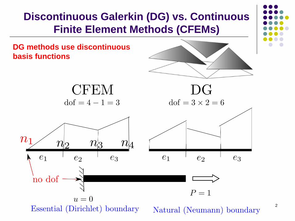
Discontinuous Galerkin (DG) vs. Continuous

Finite Element Methods (CFEMs)

DG methods use discontinuous

basis functions

2

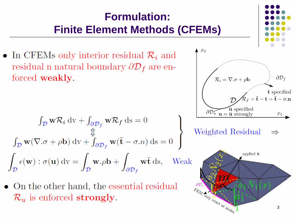
Formulation:

Finite Element Methods (CFEMs)

3

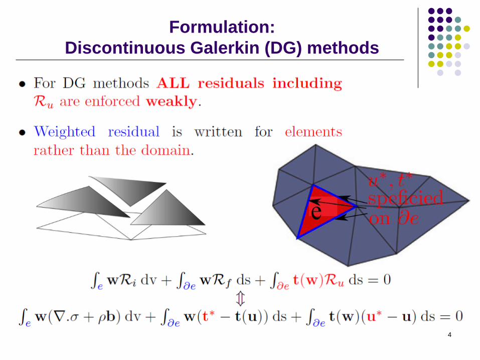
Formulation:

Discontinuous Galerkin (DG) methods

4

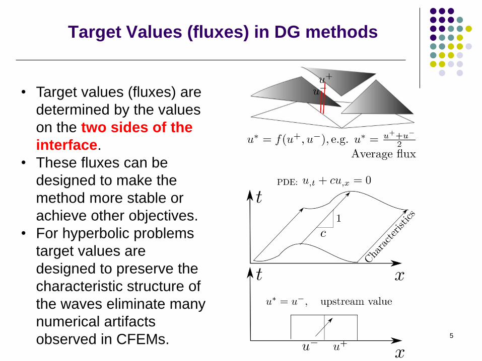
Target Values (fluxes) in DG methods

• Target values (fluxes) are

determined by the values

on the two sides of the

interface.

• These fluxes can be

designed to make the

method more stable or

achieve other objectives.

• For hyperbolic problems

target values are

designed to preserve the

characteristic structure of

the waves eliminate many

numerical artifacts

observed in CFEMs. 5

Comparison of CFEM and DG methods:• Advantages of CFEMs

• Preliminaries

• Advantages of DG methods

6

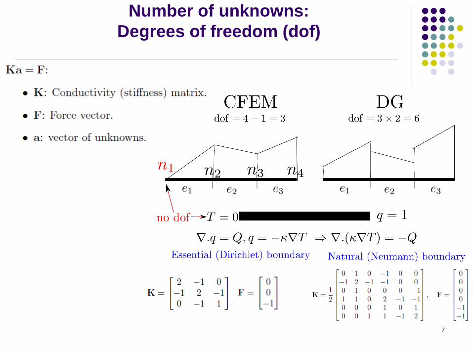
Number of unknowns:

Degrees of freedom (dof)

7

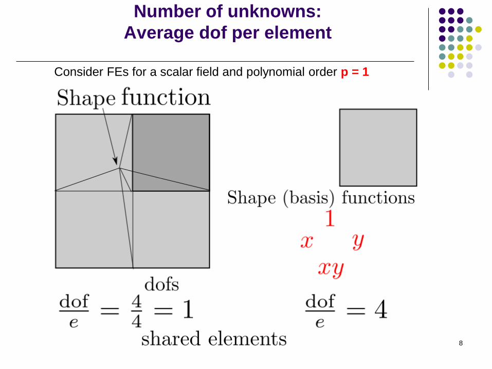
Number of unknowns:

Average dof per element

Consider FEs for a scalar field and polynomial order p = 1

8

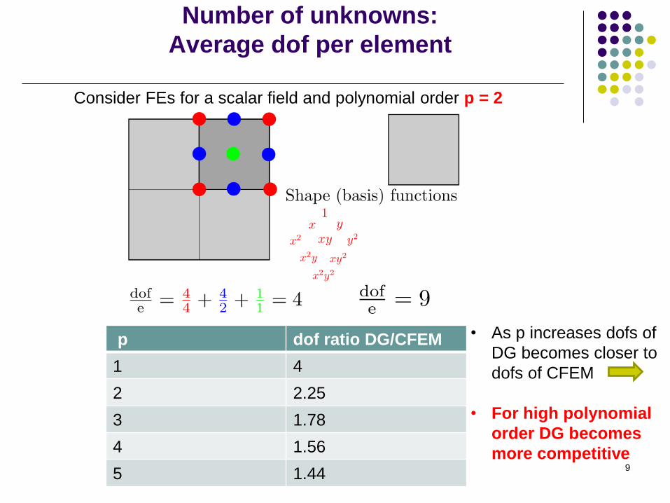
Number of unknowns:

Average dof per element

Consider FEs for a scalar field and polynomial order p = 2

p dof ratio DG/CFEM

1 4

2 2.25

3 1.78

4 1.56

5 1.44

• As p increases dofs of

DG becomes closer to

dofs of CFEM

• For high polynomial

order DG becomes

more competitive9

Comparison of CFEM and DG methods:• Advantages of CFEMs

• Preliminaries

• Advantages of DG methods

10

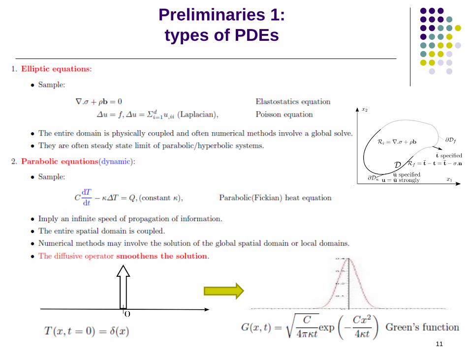
Preliminaries 1:

types of PDEs

11

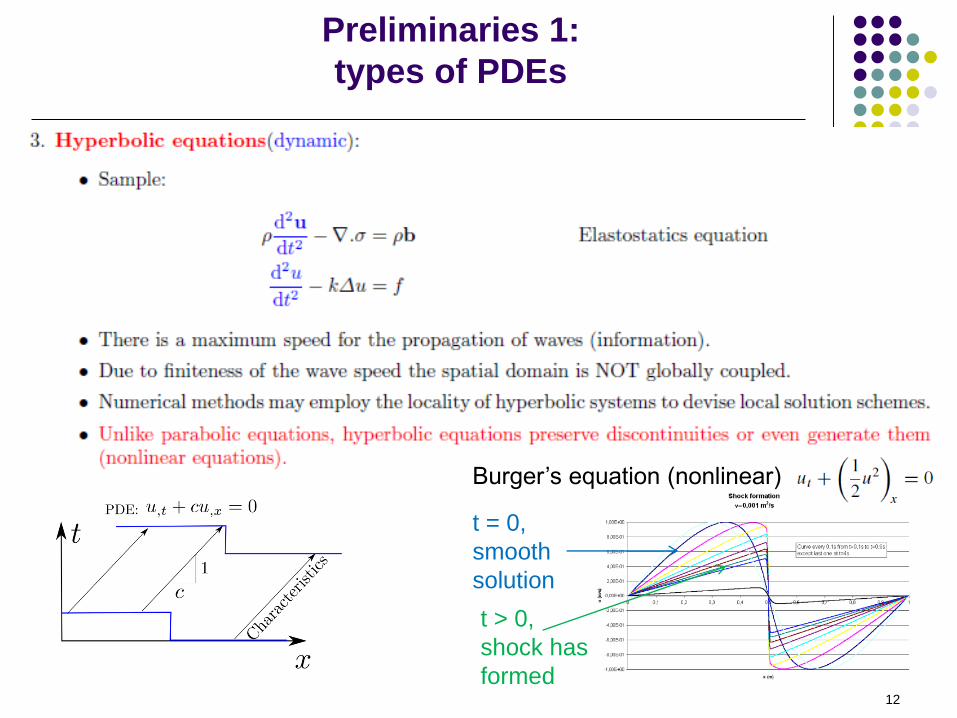
t = 0,

smooth

solution

t > 0,

shock has

formed

Burger’s equation (nonlinear)

Preliminaries 1:

types of PDEs

12

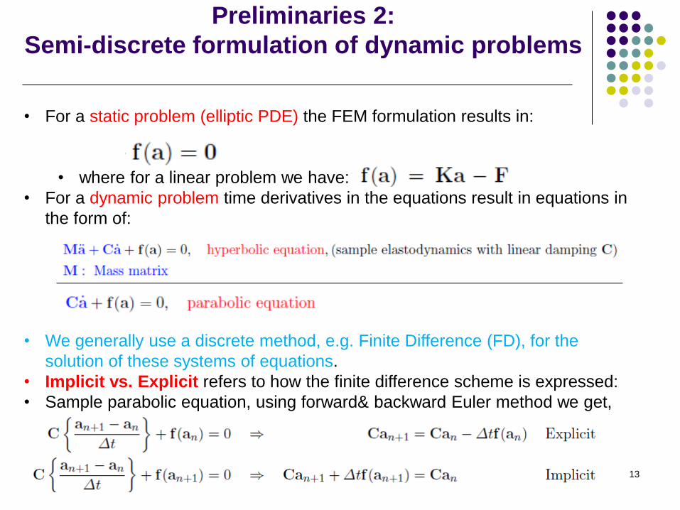
Preliminaries 2:

Semi-discrete formulation of dynamic problems

• For a static problem (elliptic PDE) the FEM formulation results in:

• where for a linear problem we have:

• For a dynamic problem time derivatives in the equations result in equations in

the form of:

• We generally use a discrete method, e.g. Finite Difference (FD), for the

solution of these systems of equations.

• Implicit vs. Explicit refers to how the finite difference scheme is expressed:

• Sample parabolic equation, using forward& backward Euler method we get,

13

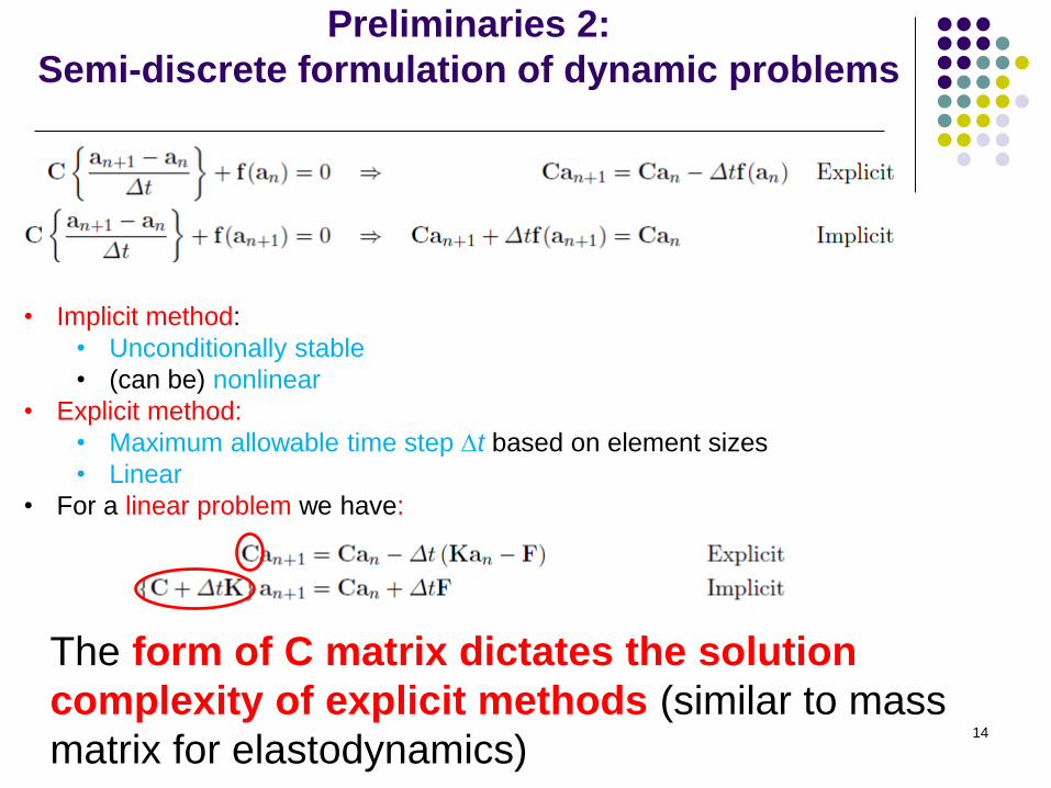
Preliminaries 2:

Semi-discrete formulation of dynamic problems

• Implicit method:

• Unconditionally stable

• (can be) nonlinear

• Explicit method:

• Maximum allowable time step Dt based on element sizes

• Linear

• For a linear problem we have:

The form of C matrix dictates the solution

complexity of explicit methods (similar to mass

matrix for elastodynamics)14

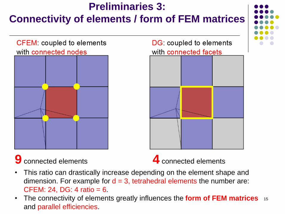
Preliminaries 3:

Connectivity of elements / form of FEM matrices

9 connected elements 4 connected elements

• This ratio can drastically increase depending on the element shape and

dimension. For example for d = 3, tetrahedral elements the number are:

CFEM: 24, DG: 4 ratio = 6.

• The connectivity of elements greatly influences the form of FEM matrices

and parallel efficiencies.

15

Comparison of CFEM and DG methods:• Advantages of CFEMs

• Preliminaries

• Advantages of DG methods

16

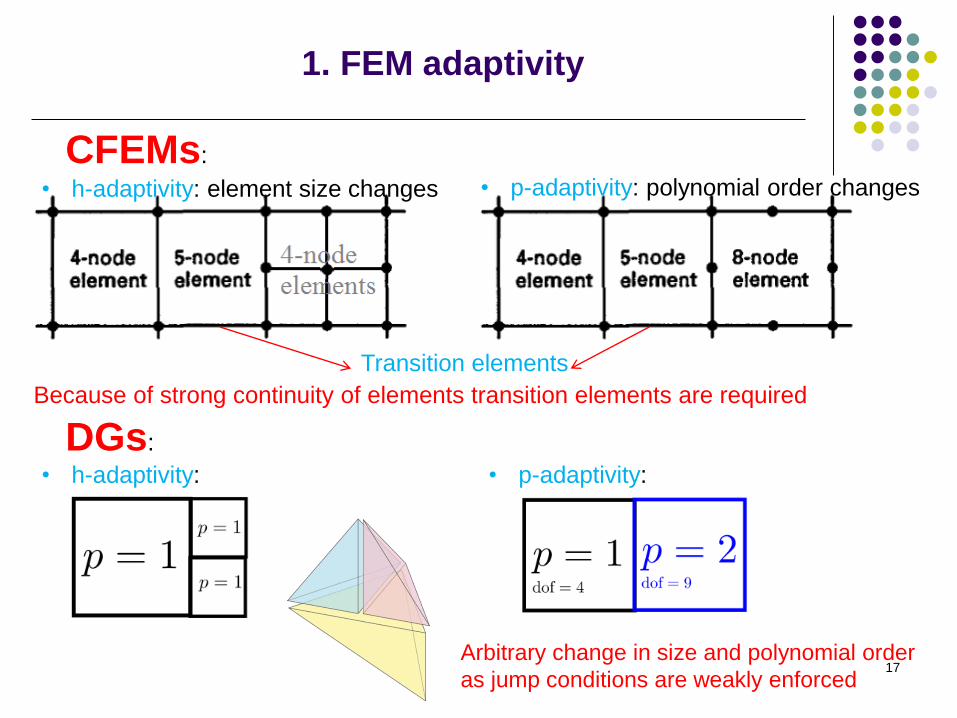
1. FEM adaptivity

CFEMs:

• h-adaptivity: element size changes • p-adaptivity: polynomial order changes

Transition elements

Because of strong continuity of elements transition elements are required

DGs:

• h-adaptivity: • p-adaptivity:

Arbitrary change in size and polynomial order

as jump conditions are weakly enforced17

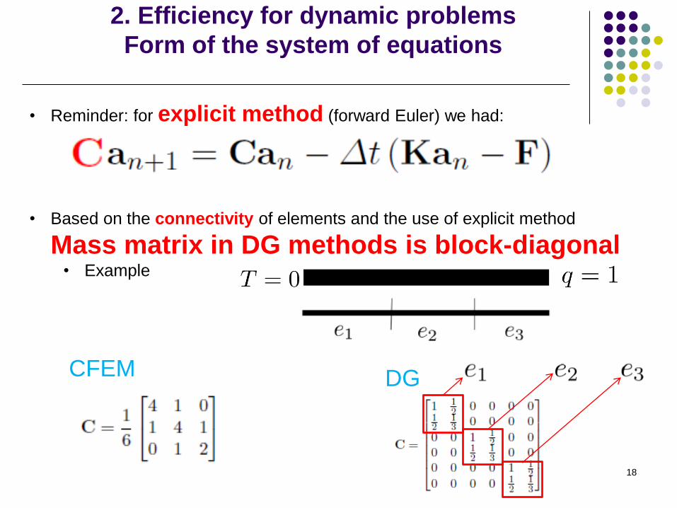
2. Efficiency for dynamic problems

Form of the system of equations

• Reminder: for explicit method (forward Euler) we had:

• Based on the connectivity of elements and the use of explicit method

Mass matrix in DG methods is block-diagonal• Example

CFEM DG

18

2. Efficiency for dynamic problems

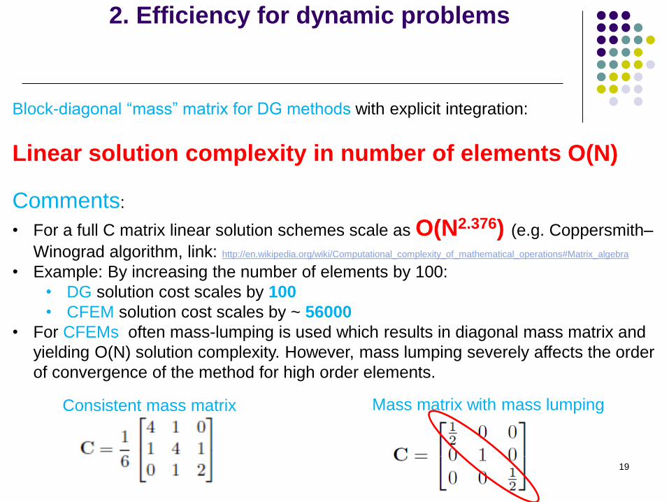
Block-diagonal “mass” matrix for DG methods with explicit integration:

Linear solution complexity in number of elements O(N)

Comments:

• For a full C matrix linear solution schemes scale as O(N2.376) (e.g. Coppersmith–

Winograd algorithm, link: http://en.wikipedia.org/wiki/Computational_complexity_of_mathematical_operations#Matrix_algebra

• Example: By increasing the number of elements by 100:

• DG solution cost scales by 100

• CFEM solution cost scales by ~ 56000

• For CFEMs often mass-lumping is used which results in diagonal mass matrix and

yielding O(N) solution complexity. However, mass lumping severely affects the order

of convergence of the method for high order elements.

Consistent mass matrix Mass matrix with mass lumping

19

3. Parallel computing

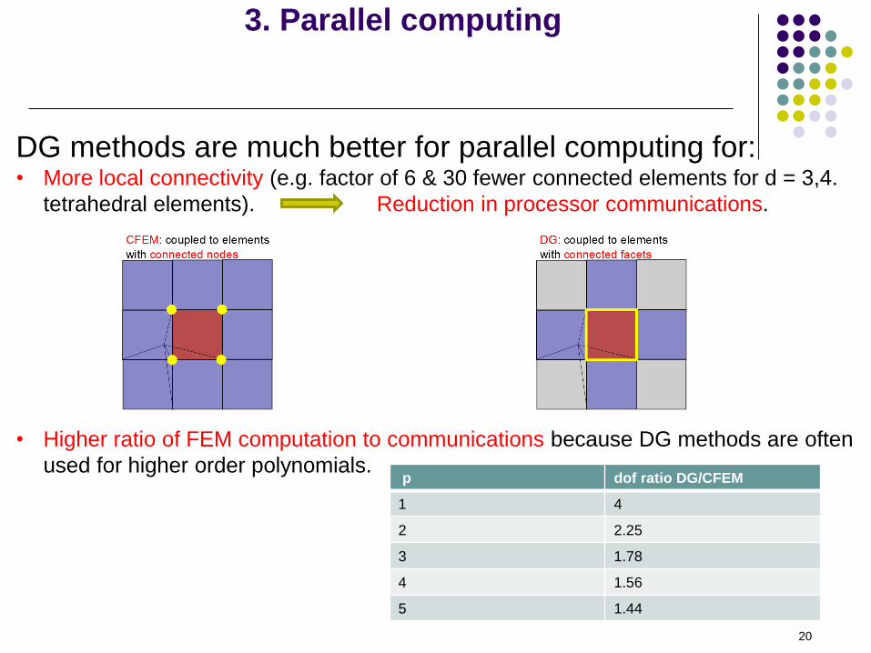
DG methods are much better for parallel computing for:• More local connectivity (e.g. factor of 6 & 30 fewer connected elements for d = 3,4.

tetrahedral elements). Reduction in processor communications.

• Higher ratio of FEM computation to communications because DG methods are often

used for higher order polynomials.p dof ratio DG/CFEM

1 4

2 2.25

3 1.78

4 1.56

5 1.44

20

4. Resolving shocks and discontinuities for

hyperbolic problems

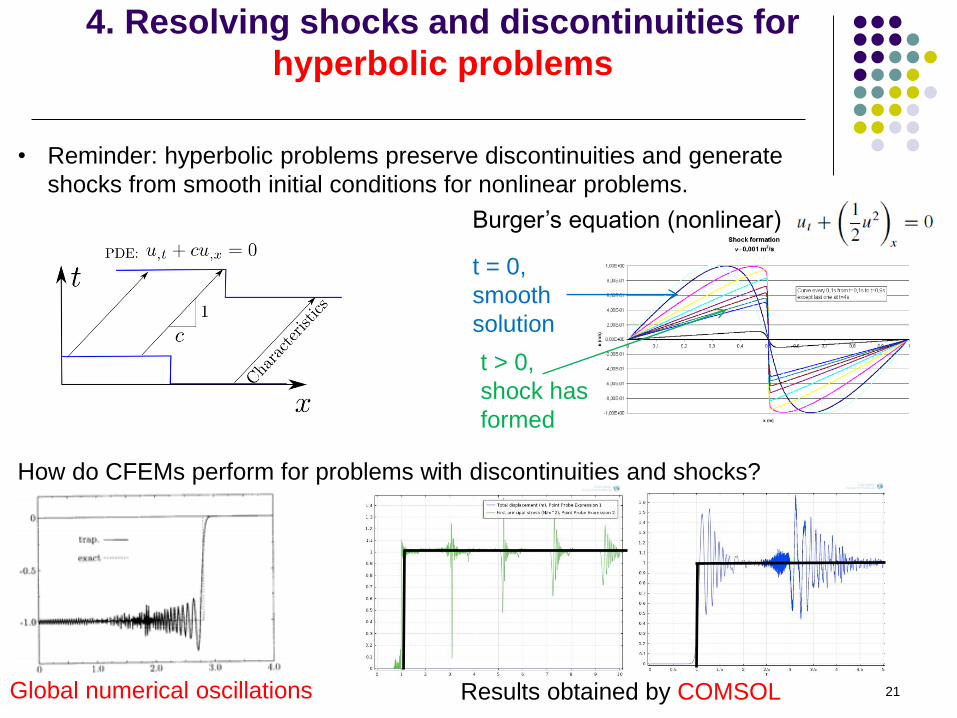
• Reminder: hyperbolic problems preserve discontinuities and generate

shocks from smooth initial conditions for nonlinear problems.

How do CFEMs perform for problems with discontinuities and shocks?

t = 0,

smooth

solution

t > 0,

shock has

formed

Burger’s equation (nonlinear)

Global numerical oscillations Results obtained by COMSOL 21

4. Resolving shocks and discontinuities for

hyperbolic problems

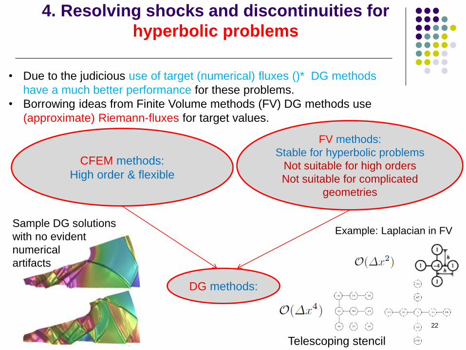
• Due to the judicious use of target (numerical) fluxes ()* DG methods

have a much better performance for these problems.

• Borrowing ideas from Finite Volume methods (FV) DG methods use

(approximate) Riemann-fluxes for target values.

CFEM methods:

High order & flexible

FV methods:

Stable for hyperbolic problems

Not suitable for high orders

Not suitable for complicated

geometries

DG methods:

Example: Laplacian in FV

Telescoping stencil

Sample DG solutions

with no evident

numerical

artifacts

22

5. Recovering balance laws at the element

level

Since the weight functions can be set to unity at each

individual element, balance properties can be recovered

at element level.

23

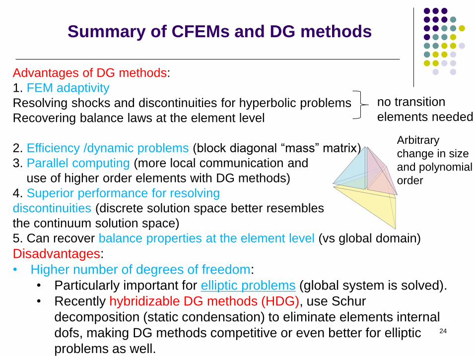
Advantages of DG methods:

1. FEM adaptivity

Resolving shocks and discontinuities for hyperbolic problems

Recovering balance laws at the element level

2. Efficiency /dynamic problems (block diagonal “mass” matrix)

3. Parallel computing (more local communication and

use of higher order elements with DG methods)

4. Superior performance for resolving

discontinuities (discrete solution space better resembles

the continuum solution space)

5. Can recover balance properties at the element level (vs global domain)

Disadvantages:

• Higher number of degrees of freedom:

• Particularly important for elliptic problems (global system is solved).

• Recently hybridizable DG methods (HDG), use Schur

decomposition (static condensation) to eliminate elements internal

dofs, making DG methods competitive or even better for elliptic

problems as well.

no transition

elements needed

Arbitrary

change in size

and polynomial

order

Summary of CFEMs and DG methods

24