Comparison of Boosting and Partial Least Squares Techniques for Real-time Pattern

Recognition of Brain Activation in Functional Magnetic Resonance Imaging

H. Davis1,2, S. Posse2, E. C. Witting2, and P. Soliz1,2

1. VisionQuest Biomedical, LLC2. University of New Mexico

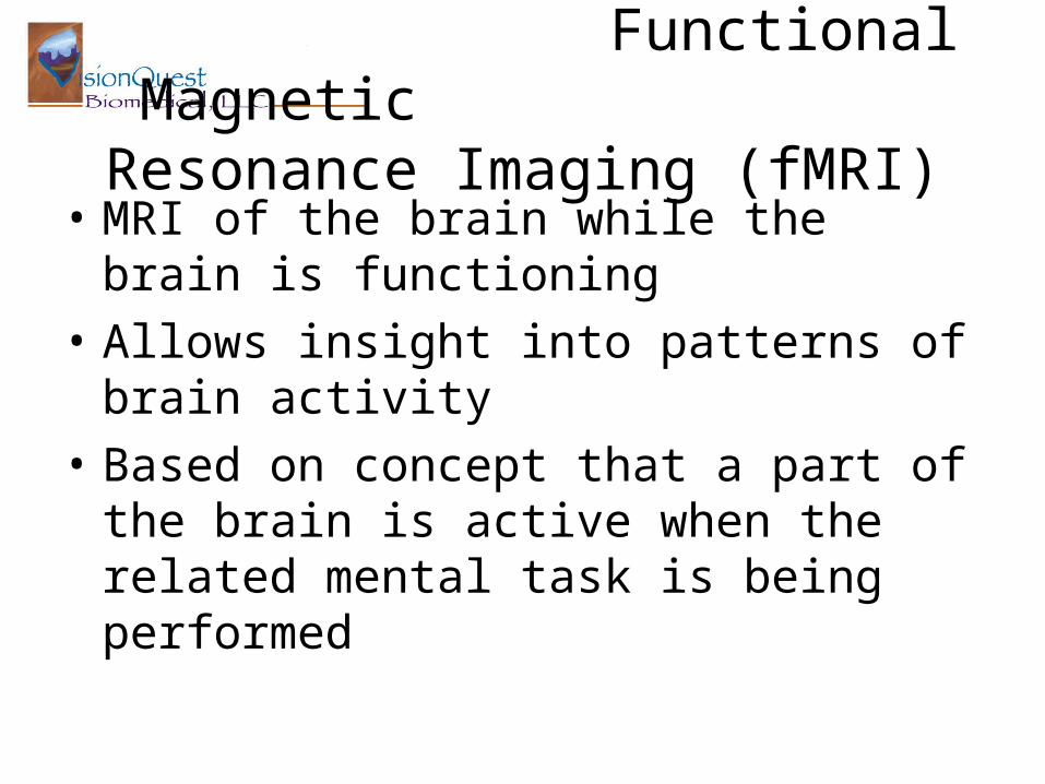
Functional Magnetic Resonance Imaging (fMRI)

• MRI of the brain while the brain is functioning• Allows insight into patterns of brain activity• Based on concept that a part of the brain is

active when the related mental task is being performed

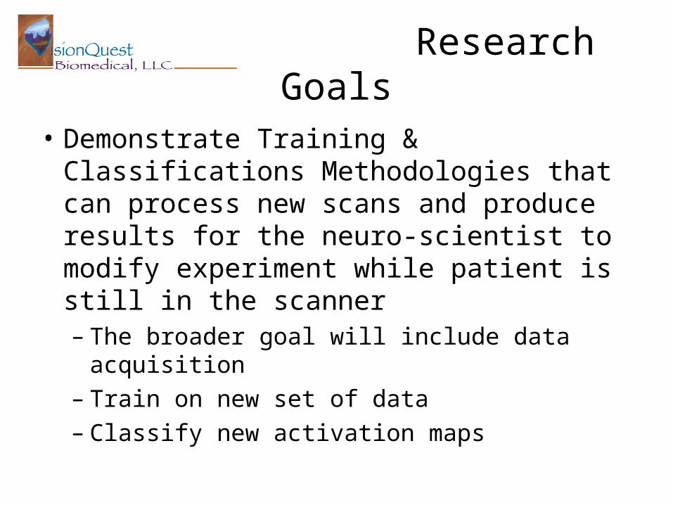
Research Goals

• Demonstrate Training & Classifications Methodologies that can process new scans and produce results for the neuro-scientist to modify experiment while patient is still in the scanner– The broader goal will include data acquisition– Train on new set of data– Classify new activation maps

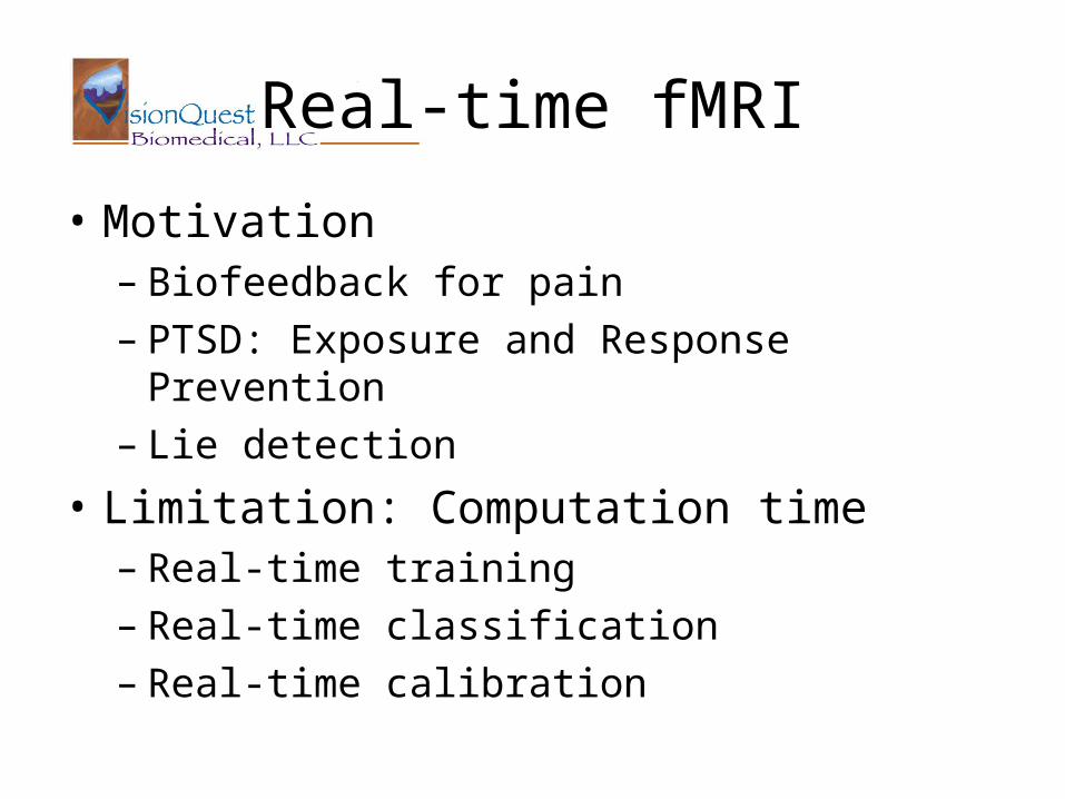
Real-time fMRI

• Motivation– Biofeedback for pain– PTSD: Exposure and Response Prevention– Lie detection

• Limitation: Computation time– Real-time training– Real-time classification– Real-time calibration

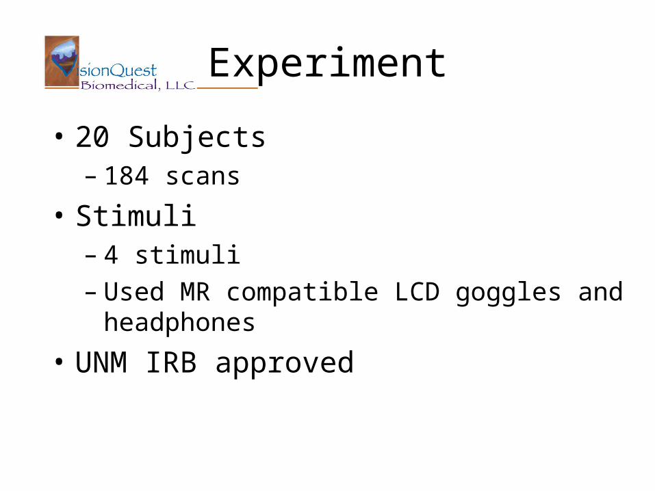
Experiment

• 20 Subjects– 184 scans

• Stimuli– 4 stimuli– Used MR compatible LCD goggles and headphones

• UNM IRB approved

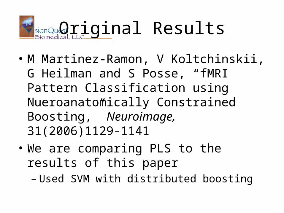
Original Results

• M Martinez-Ramon, V Koltchinskii, G Heilman and S Posse, “fMRI Pattern Classification using Nueroanatomically Constrained Boosting,” Neuroimage, 31(2006)1129-1141

• We are comparing PLS to the results of this paper– Used SVM with distributed boosting

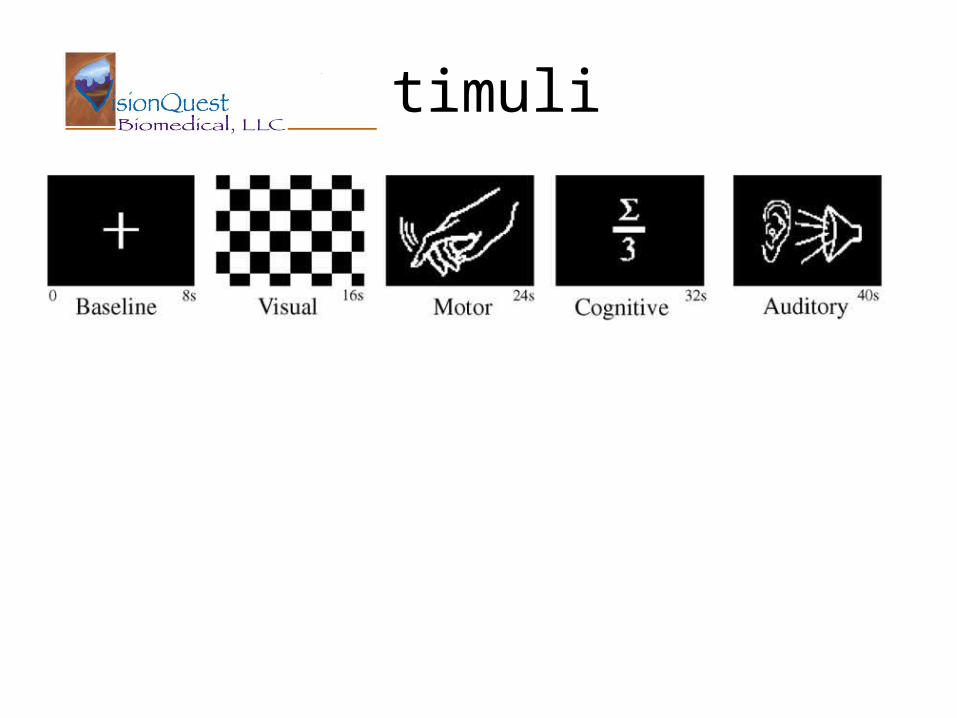
Stimuli

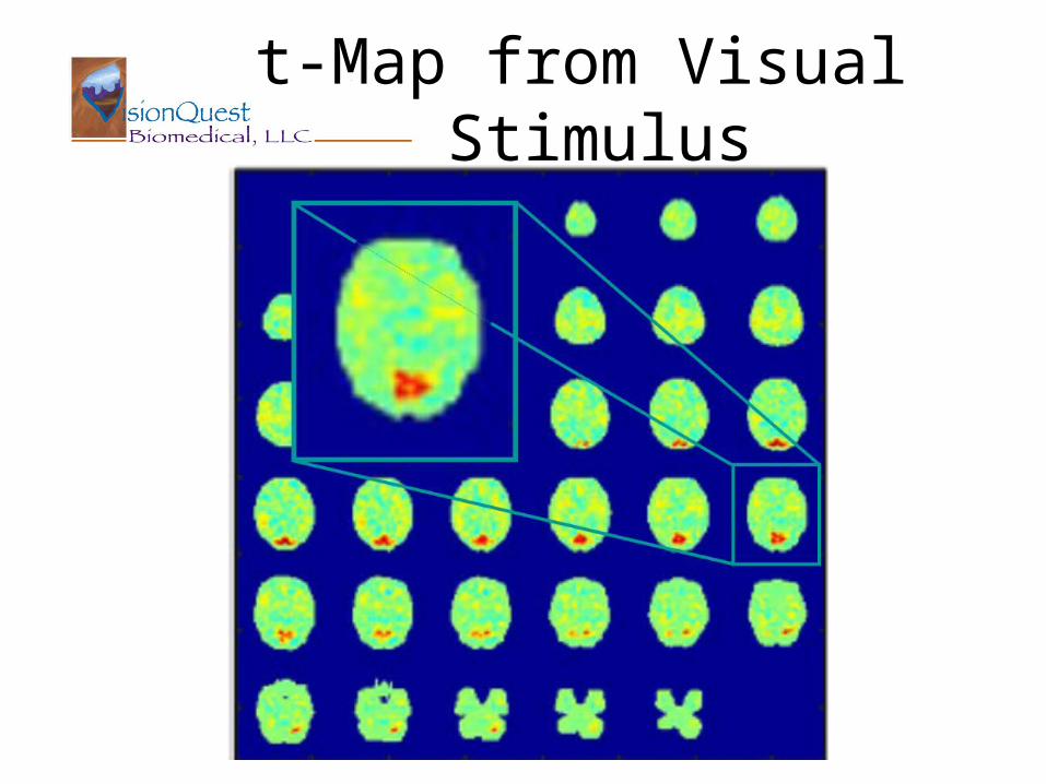
t-Map from Visual Stimulus

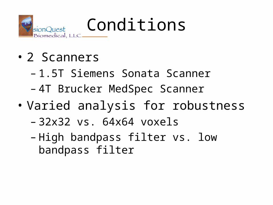
Conditions

• 2 Scanners– 1.5T Siemens Sonata Scanner– 4T Brucker MedSpec Scanner

• Varied analysis for robustness– 32x32 vs. 64x64 voxels– High bandpass filter vs. low bandpass filter

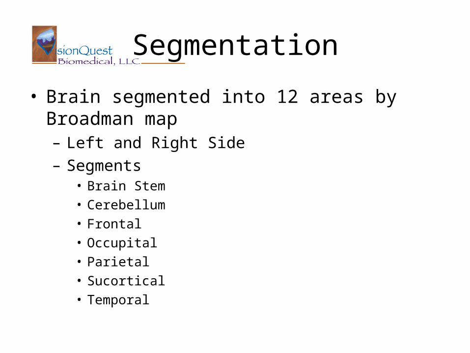
Segmentation

• Brain segmented into 12 areas by Broadman map– Left and Right Side– Segments

• Brain Stem• Cerebellum• Frontal• Occupital• Parietal• Sucortical• Temporal

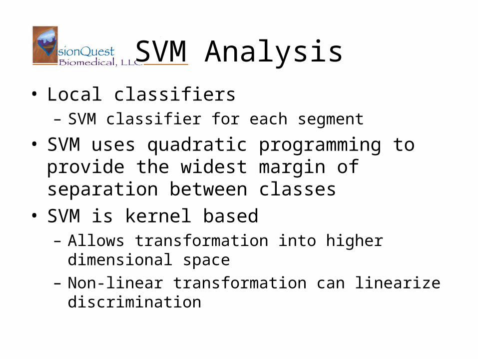
SVM Analysis• Local classifiers– SVM classifier for each segment

• SVM uses quadratic programming to provide the widest margin of separation between classes

• SVM is kernel based– Allows transformation into higher dimensional space– Non-linear transformation can linearize discrimination

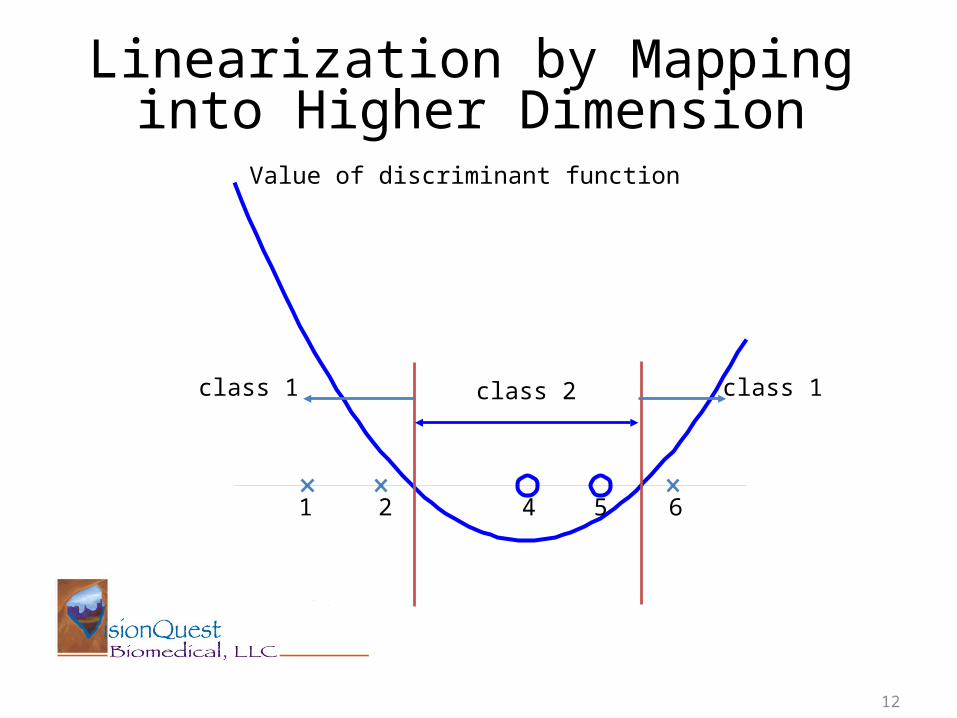
Linearization by Mapping into Higher Dimension

12

Value of discriminant function

1 2 4 5 6

class 2 class 1class 1

Boosting

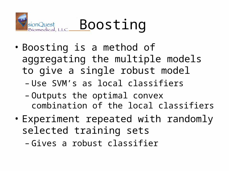
• Boosting is a method of aggregating the multiple models to give a single robust model– Use SVM’s as local classifiers– Outputs the optimal convex combination of the

local classifiers

• Experiment repeated with randomly selected training sets– Gives a robust classifier

Linear Regression

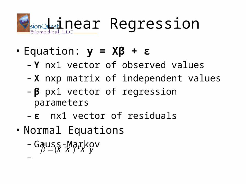
• Equation: y = Xβ + ε – Y nx1 vector of observed values– X nxp matrix of independent values– β px1 vector of regression parameters– ε nx1 vector of residuals

• Normal Equations– Gauss-Markov– yXXX ')'( 1

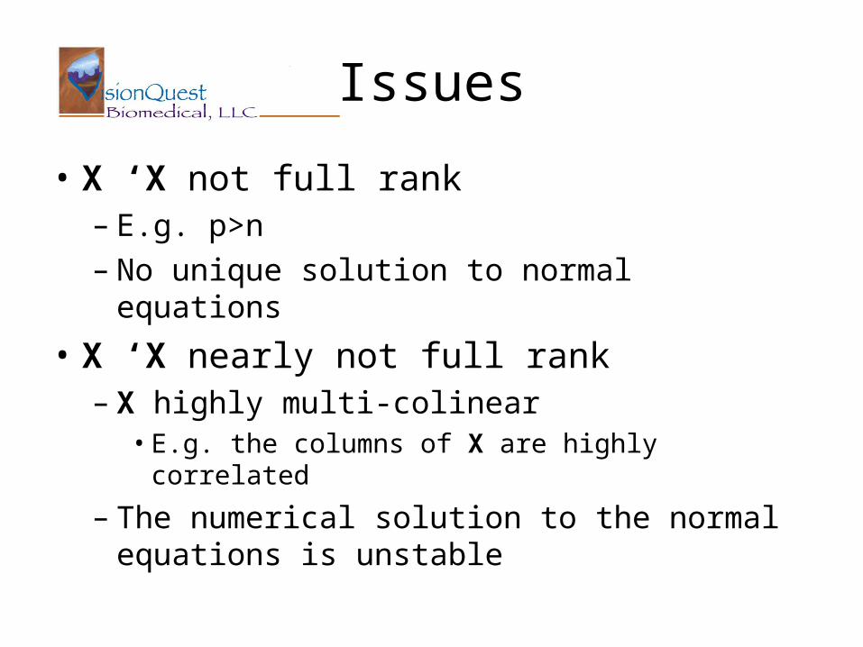
Issues

• X ‘X not full rank– E.g. p>n– No unique solution to normal equations

• X ‘X nearly not full rank– X highly multi-colinear• E.g. the columns of X are highly correlated

– The numerical solution to the normal equations is unstable

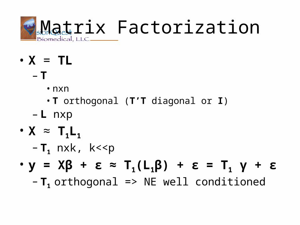
Matrix Factorization

• X = TL– T • nxn• T orthogonal (T’T diagonal or I)

– L nxp• X ≈ T1L1

– T1 nxk, k<<p

• y = Xβ + ε ≈ T1(L1β) + ε = T1 γ + ε – T1 orthogonal => NE well conditioned

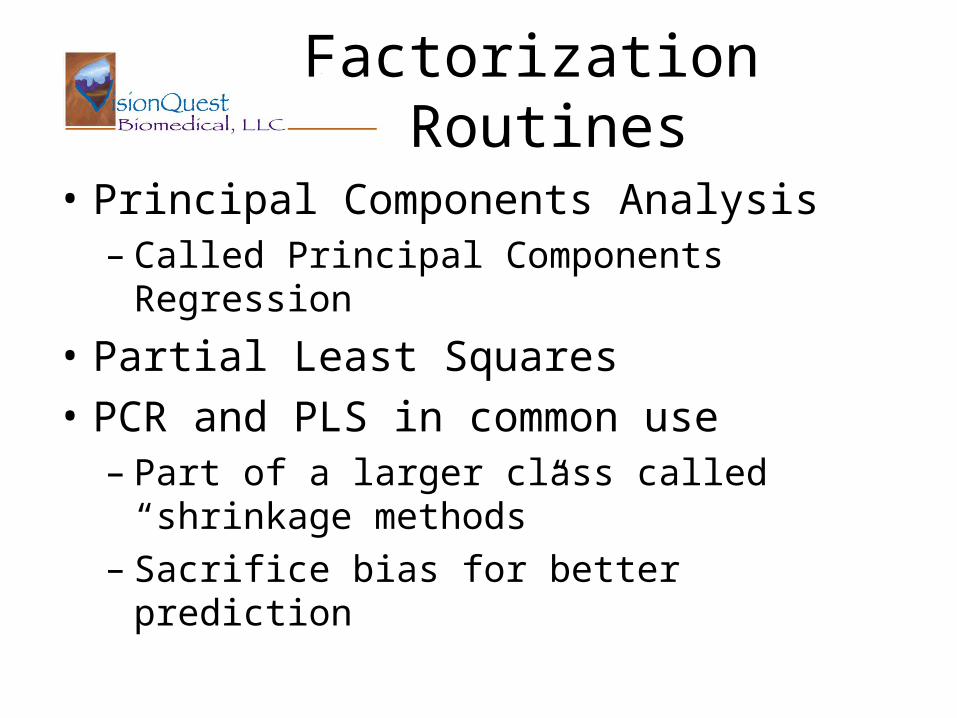
Factorization Routines

• Principal Components Analysis– Called Principal Components Regression

• Partial Least Squares• PCR and PLS in common use– Part of a larger class called “shrinkage methods”– Sacrifice bias for better prediction

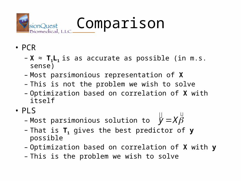
Comparison

• PCR– X ≈ T1L1 is as accurate as possible (in m.s. sense)– Most parsimonious representation of X– This is not the problem we wish to solve– Optimization based on correlation of X with itself

• PLS– Most parsimonious solution to– That is T1 gives the best predictor of y possible– Optimization based on correlation of X with y– This is the problem we wish to solve

Xy

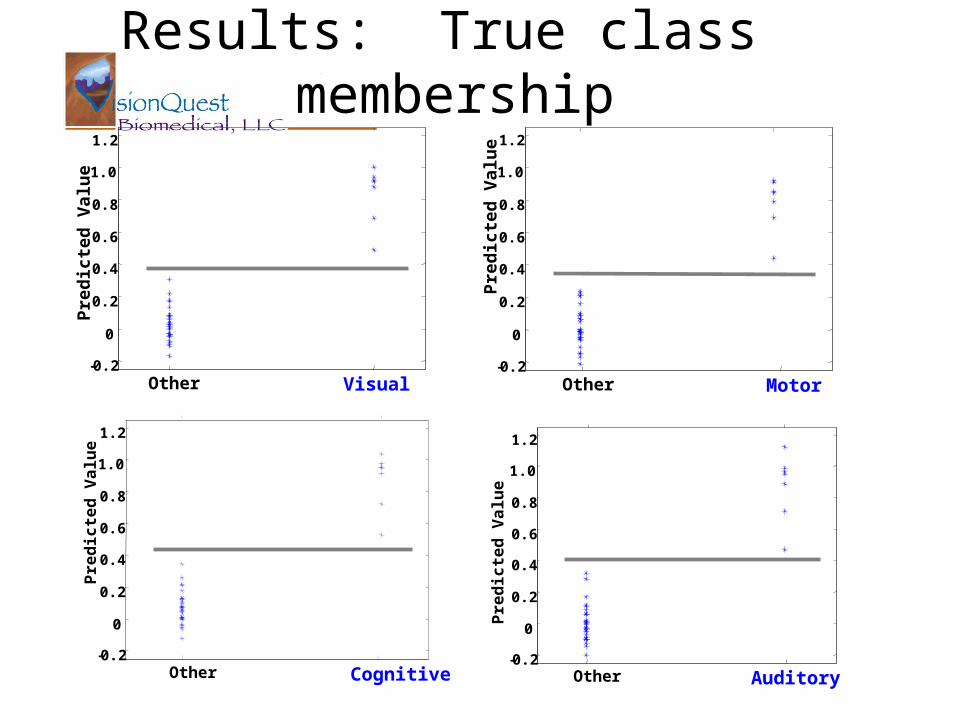
Results: True class membership

Other Cognitive-0.2

0

0.2

0.4

0.6

0.8

1.0

1.2

Pre

dic

ted

Va

lue

Other Visual-0.2

0

0.2

0.4

0.6

0.8

1.0

1.2

Pre

dic

ted

Val

ue

Other Motor-0.2

0

0.2

0.4

0.6

0.8

1.0

1.2

Pre

dic

ted

Val

ue

Other Auditory-0.2

0

0.2

0.4

0.6

0.8

1.0

1.2

Pre

dic

ted

Va

lue

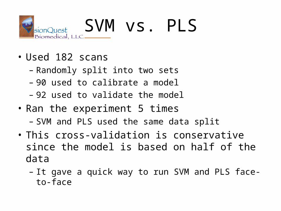
SVM vs. PLS

• Used 182 scans– Randomly split into two sets– 90 used to calibrate a model– 92 used to validate the model

• Ran the experiment 5 times– SVM and PLS used the same data split

• This cross-validation is conservative since the model is based on half of the data– It gave a quick way to run SVM and PLS face-to-face

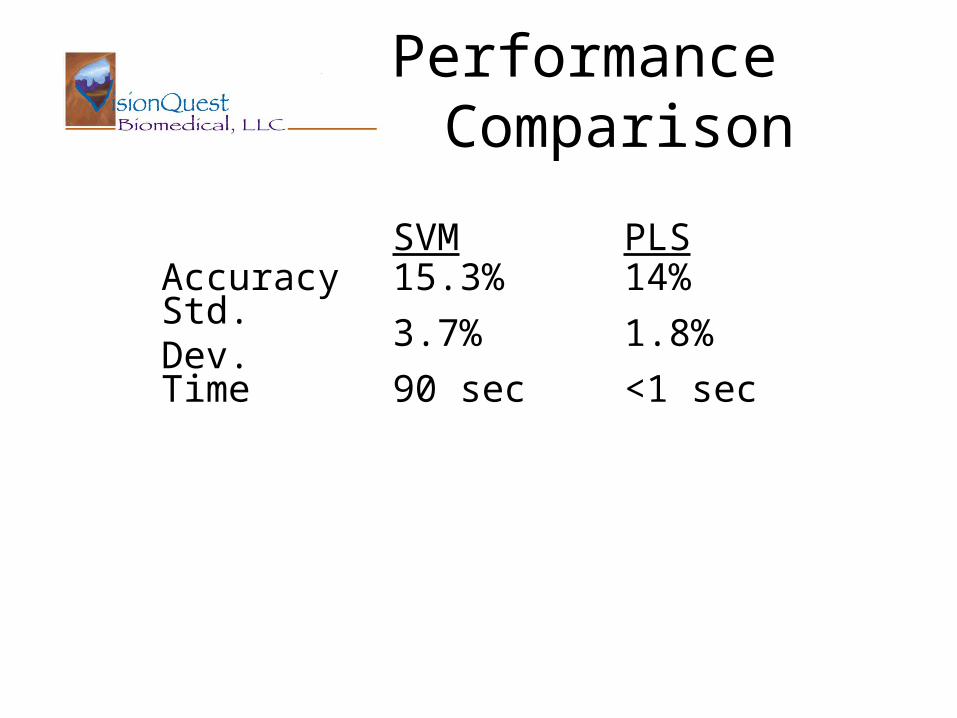
Performance Comparison

AccuracyStd. Dev.Time

15.3%3.7%90 sec

14%1.8%<1 sec

SVM PLS

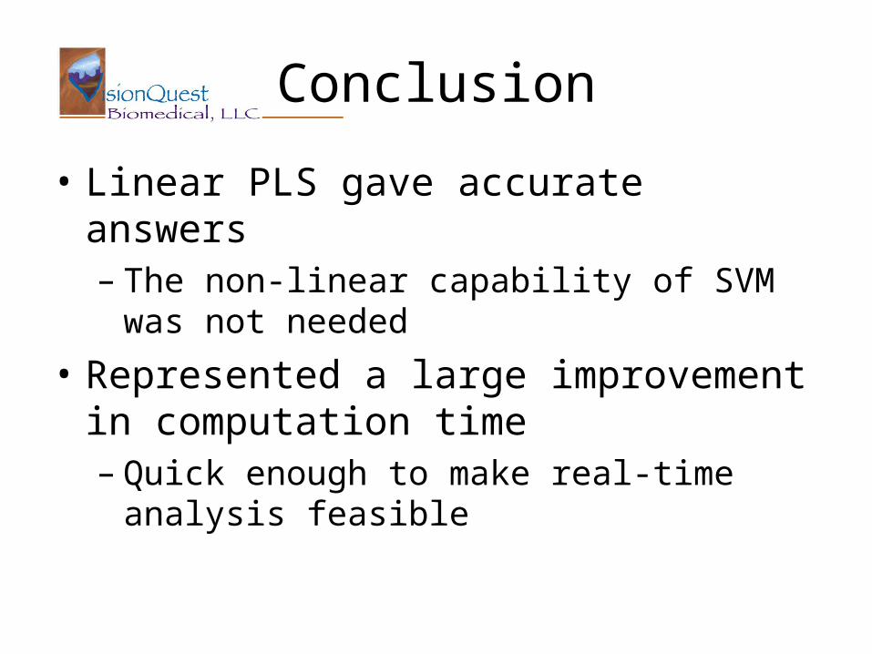
Conclusion

• Linear PLS gave accurate answers– The non-linear capability of SVM was not needed

• Represented a large improvement in computation time– Quick enough to make real-time analysis feasible