Embed Size (px)
Citation preview
COMPARISON OF ABAQUS AND EPIC NONLINEAR TRANSIENT DYNAMICMODELS FOR A HYDROGEN BURN EVENT OF HANFORD SITE HIGH-LEVEL-
WASTE TANK 241-SY-101
by
Edward A. RodriguezNuclear Systems Design & Analysis GroupTechnology & Safety Assessment Division
Los Alamos National LaboratoryLos Alamos, NM 87545
and
Rich F. DavidsonMargaret L. Walsh
Engineering Analysis GroupEngineering Sciences & Applications Division
Los Alamos National LaboratoryLos Alamos, NM 87545
October 1995
Report No.
LA-UR-95-3441
Los Alamos National LaboratoryLos Alamos National Laboratory
LA-UR-95-3441
1
COMPARISON OF ABAQUS AND EPIC NONLINEAR TRANSIENT DYNAMICMODELS FOR A HYDROGEN BURN EVENT OF HANFORD SITE HIGH-LEVEL-
WASTE TANK 241-SY-101
by
Edward A. Rodriguez, Rich F. Davidson, and Margaret L. Walsh
ABSTRACT
The Hanford Site in Richland, Washington, contains repositories of high-level waste (HLW) in underground double-shell (steel) tanks (DSTs).Some of these tanks continue to exhibit large episodic releases offlammable and toxic gases. Concentrations of hydrogen gas thatpotentially may be above the lower flammability limit create a majorsafety concern, with possible consequences being in-tank burns(deflagrations) or detonations. The integrity of these DSTs is imperativeto maintaining the containment of radioactive waste, assuring structuralsurvivability, and minimizing worker/public exposure from accidentalradiological and toxicological release. As such, knowledge of the tank’sstructural response during one of these events provides a safety basis forcontinuing in-tank operations. The current safety assessment (SA) ofHLW Tank 101-SY for a hydrogen burn has been performed with ageneral-purpose, implicit finite-element-analysis (FEA) code. However,consequences of severe dynamic events cannot be assessed completelywith implicit FEA codes because of their inherent limitations. Othermethods must be employed to complete the assessment of structuraldamage when the loading is severe enough to produce extensive materialfailure. Advanced transient dynamic, nonlinear hydrodynamic codes lendthemselves to this type of problem because of the overall integration ofconstitutive material models, equations of state, and failure and damagemodels. This paper focuses on comparing FEA model results between theABAQUS implicit FEA code and the EPIC explicit hydrodynamic code foran arbitrary hydrogen burn event causing a transient pressurization ofthe primary steel liner in HLW Tank 101-SY. The results are used to(1) qualify the accuracy of the ABAQUS code used in the SA of HLW Tank101-SY for hydrogen burn events and (2) qualify the EPIC code to extendinto the very high strain and strain-rate regime and extend into high-pressures for detonation events. We conclude that both ABAQUS andEPIC provide astonishingly accurate results and correlate extremely well(within 10%) for the burn event pressurization. These results areconsidered valid through the transient until soil overburden separationoccurs. Currently, ABAQUS results are not valid because the modelingtechnique does not allow for soil separation and reimpaction. However,EPIC provides a qualitative and quantitative means to predict damagecaused by soil separation and subsequent reimpaction on the tank dome.
LA-UR-95-3441
2
1.0. INTRODUCTION
A major safety concern with high-level waste (HLW) Tank 101-SY is the continuedstructural integrity of the primary and secondary steel liner containments and thereinforced concrete structure when subjected to a potential hydrogen burn event. Thesafety concern has been addressed and reported in a Los Alamos National Laboratory(LANL) safety assessment (SA)1 based on detailed nonlinear finite element analyses(FEA) of the structure under dynamic pressure loadings. The structural analyses wereconducted with the implicit FEA code ABAQUS,2 which predicted the nonlinearresponse based on a transient pressure pulse caused by a hydrogen burn event.Although the ABAQUS FEA model results of HLW Tank 101-SY generally have beenaccepted by external oversight committees and internal review panels, it was evidentthat the limits of the code were being tested with the high-strain rates and consequentlywith the high overall strains for a postulated burn transient. Therefore, ABAQUSwould not be capable of predicting structural responses for very high pressures orpressurization rates.
Furthermore, questions have been raised as to the ultimate collapse capacity of thedome structure, as well as the overall structural consequences of a potential energeticburn (deflagration) of released flammable gases. Although the ABAQUS FEA code maypredict large deformations, high-strain conditions, and concrete cracking under adynamic loading accurately, it cannot predict very high strains, overall damage, or lossof material during the progression of material failure. As such, to investigate theconsequences of severe structural damage properly, strains of 75 to 100% with severematerial damage must be predicted accurately. Obviously, these conditions are wellbeyond the limits of the ABAQUS implicit code or any other implicit FEA code.
Therefore, LANL has chosen to provide a comparison of ABAQUS results with theexplicit FEA hydrodynamic code EPIC3 to obtain a qualitative measure of
1. the accuracy of the ABAQUS code used in the SA of HLW Tank 101-SY forhydrogen burn events, and
2. the EPIC code to extend into the very high strain and material failure regimefor detonation events.
EPIC is a specialized multidimensional Lagrangian hydrodynamic FEA code that solvesthe equations of motions explicitly, providing a measure of the structural response wellbeyond normal limits of an implicit FEA code. The code is extremely versatile for casesinvolving high-velocity impact and hypervelocity conditions. Constitutive materialmodeling of stress and strain within EPIC is subdivided into the hydrostatic anddeviatoric parts. The hydrostatic part, which is the average of the mean stress(pressure) and mean strain (volume), is related through an equation of state andthereby properly considers thermodynamic effects.4 The deviatoric parts, or shearstress and shear strain, include the description of the plastic behavior of the material, aswell as any strain-rate effects. Material failure criteria also are employed. Total damageand material loss therefore are accounted for incrementally throughout the analysis.
LA-UR-95-3441
3
This differs from implicit FEA codes in that the hydrostatic part of the constitutivematerial model does not contain an equation-of-state model or a material failure model.
2.0. BACKGROUND
The Hanford Site in Richland, Washington, stores large repositories of HLW, which hasaccumulated from the chemical separation processing of defense reactor irradiated fuelsfor plutonium recovery. This waste, which consists of liquids and precipitated solids,undergoes radiolytic decay, whereas organics in the waste undergo thermal chemicalreactions. The effects of radiolytic decay and thermal chemical reactions tend togenerate flammable and toxic gases. The flammable gas issue was declared anunreviewed safety question (USQ) for Tank 101-SY in March 1990. The USQ wasgenerated initially by a concern over the simultaneous generation of fuel (hydrogen)and an oxidizer (nitrous oxide). However, extensive analytical and experimental effortsinitiated as a result of the declaration of the USQ were expanded to consider also thegeneration of other flammable gases, namely ammonia and methane. Since then,several other single-shell and double-shell tanks have been placed on the FlammableGas Watchlist as potential hydrogen gas-generating tanks. These are considered aPriority 1 safety issue.
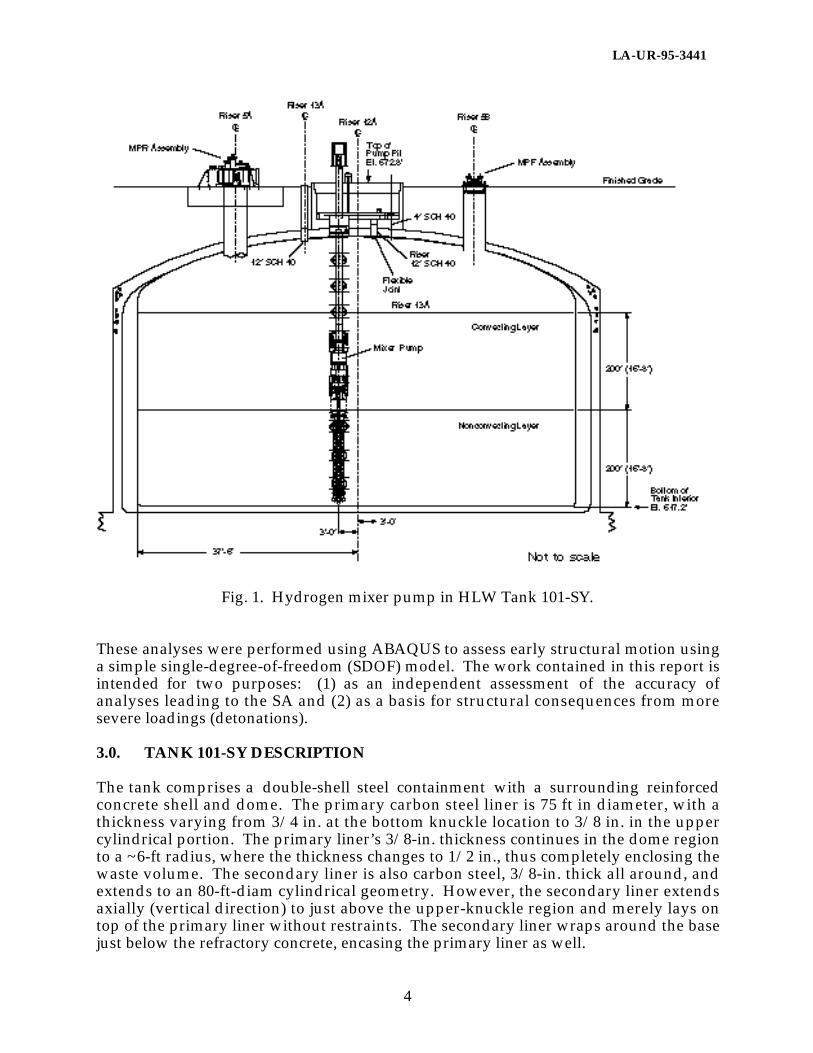
When the issue of the USQ was declared, a program was initiated by WestinghouseHanford Company (WHC) to begin in-tank monitoring efforts of Tank 101-SY todetermine waste characterization, gas species and concentrations, waste temperature,etc. The waste characteristics were such that flammable and toxic gases were beinggenerated; this produced large episodic releases of hydrogen (H2) every ~120 days,with a hydrogen concentration in excess of the lower flammability limit (LFL). Thiscondition posed a major safety issue because of potential burns or detonations from in-tank operations; that could cause a subsequent release of radioactivity to theatmosphere. To mitigate the large episodic releases, a pump was placed inside the tank(Fig. 1) to mix the waste continuously and release small quantities of flammable andtoxic gases effectively. LANL was tasked by the Department of Energy to provide anSA of the pump mixing operations. Among other safety issues, consequences ofradiological and toxicological releases to the atmosphere and consequences of ahydrogen burn were analyzed to determine the structural integrity of the tank. Thelargest historical gas release event (GRE) was used as the basis for the hydrogen burnevent. Results of the analysis were very disturbing in that large dome excitations(amplifications) were determined to occur during the transient. These excitations forcedthe dynamics of the problem to be highly nonlinear, with dynamic load factors in therange of 2.0.
LA-UR-95-3441
4
Fig. 1. Hydrogen mixer pump in HLW Tank 101-SY.
These analyses were performed using ABAQUS to assess early structural motion usinga simple single-degree-of-freedom (SDOF) model. The work contained in this report isintended for two purposes: (1) as an independent assessment of the accuracy ofanalyses leading to the SA and (2) as a basis for structural consequences from moresevere loadings (detonations).
3.0. TANK 101-SY DESCRIPTION
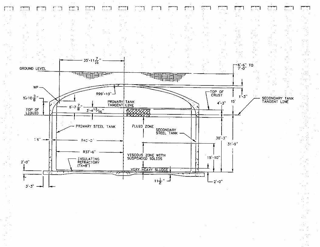
The tank comprises a double-shell steel containment with a surrounding reinforcedconcrete shell and dome. The primary carbon steel liner is 75 ft in diameter, with athickness varying from 3/4 in. at the bottom knuckle location to 3/8 in. in the uppercylindrical portion. The primary liner’s 3/8-in. thickness continues in the dome regionto a ~6-ft radius, where the thickness changes to 1/2 in., thus completely enclosing thewaste volume. The secondary liner is also carbon steel, 3/8-in. thick all around, andextends to an 80-ft-diam cylindrical geometry. However, the secondary liner extendsaxially (vertical direction) to just above the upper-knuckle region and merely lays ontop of the primary liner without restraints. The secondary liner wraps around the basejust below the refractory concrete, encasing the primary liner as well.
LA-UR-95-3441
5
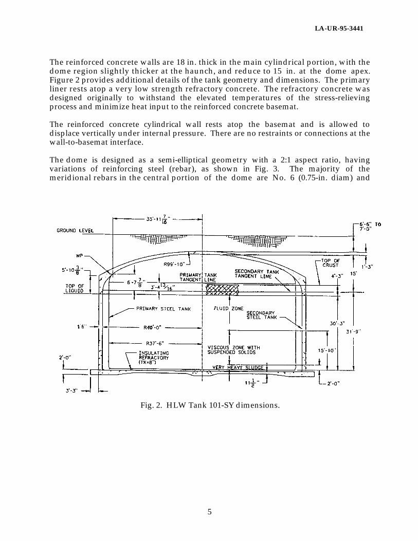
The reinforced concrete walls are 18 in. thick in the main cylindrical portion, with thedome region slightly thicker at the haunch, and reduce to 15 in. at the dome apex.Figure 2 provides additional details of the tank geometry and dimensions. The primaryliner rests atop a very low strength refractory concrete. The refractory concrete wasdesigned originally to withstand the elevated temperatures of the stress-relievingprocess and minimize heat input to the reinforced concrete basemat.
The reinforced concrete cylindrical wall rests atop the basemat and is allowed todisplace vertically under internal pressure. There are no restraints or connections at thewall-to-basemat interface.
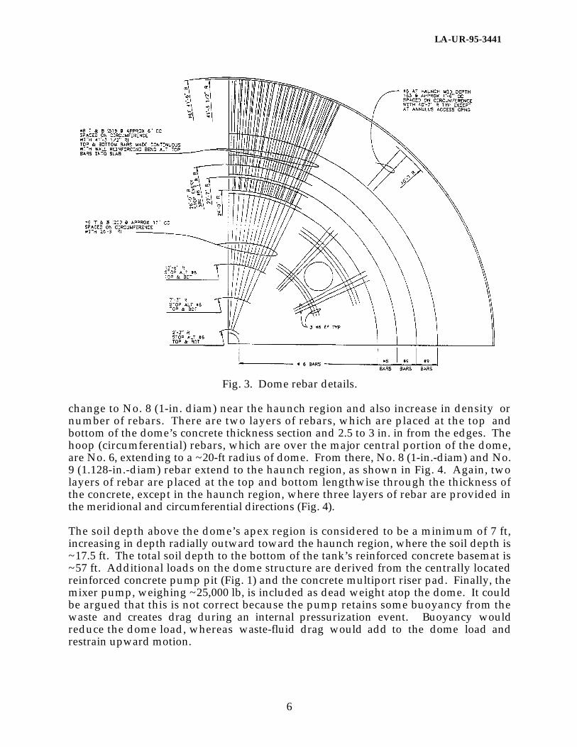
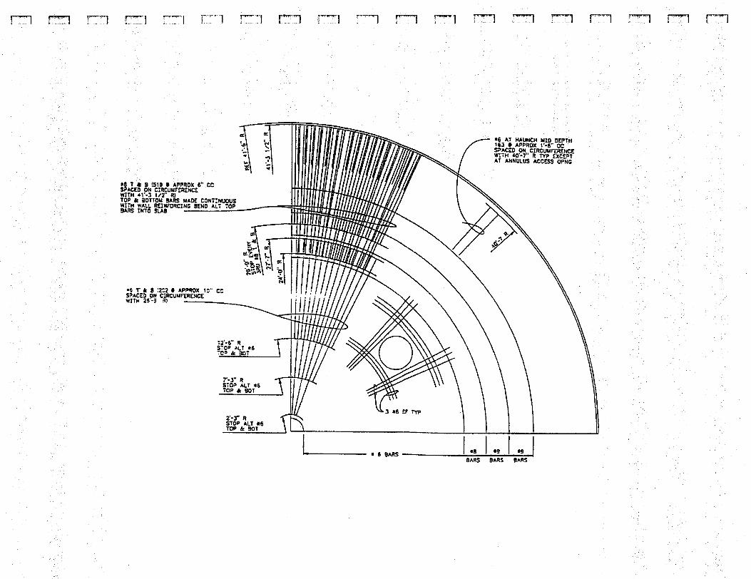
The dome is designed as a semi-elliptical geometry with a 2:1 aspect ratio, havingvariations of reinforcing steel (rebar), as shown in Fig. 3. The majority of themeridional rebars in the central portion of the dome are No. 6 (0.75-in. diam) and
Fig. 2. HLW Tank 101-SY dimensions.
LA-UR-95-3441
6
Fig. 3. Dome rebar details.
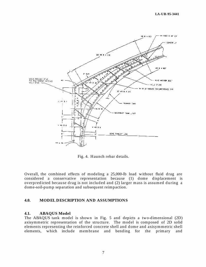
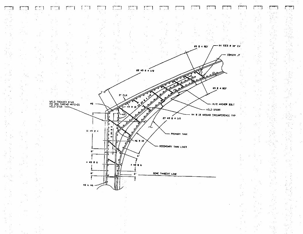
change to No. 8 (1-in. diam) near the haunch region and also increase in density ornumber of rebars. There are two layers of rebars, which are placed at the top andbottom of the dome’s concrete thickness section and 2.5 to 3 in. in from the edges. Thehoop (circumferential) rebars, which are over the major central portion of the dome,are No. 6, extending to a ~20-ft radius of dome. From there, No. 8 (1-in.-diam) and No.9 (1.128-in.-diam) rebar extend to the haunch region, as shown in Fig. 4. Again, twolayers of rebar are placed at the top and bottom lengthwise through the thickness ofthe concrete, except in the haunch region, where three layers of rebar are provided inthe meridional and circumferential directions (Fig. 4).
The soil depth above the dome’s apex region is considered to be a minimum of 7 ft,increasing in depth radially outward toward the haunch region, where the soil depth is~17.5 ft. The total soil depth to the bottom of the tank’s reinforced concrete basemat is~57 ft. Additional loads on the dome structure are derived from the centrally locatedreinforced concrete pump pit (Fig. 1) and the concrete multiport riser pad. Finally, themixer pump, weighing ~25,000 lb, is included as dead weight atop the dome. It couldbe argued that this is not correct because the pump retains some buoyancy from thewaste and creates drag during an internal pressurization event. Buoyancy wouldreduce the dome load, whereas waste-fluid drag would add to the dome load andrestrain upward motion.
LA-UR-95-3441
7
Fig. 4. Haunch rebar details.
Overall, the combined effects of modeling a 25,000-lb load without fluid drag areconsidered a conservative representation because (1) dome displacement isoverpredicted because drag is not included and (2) larger mass is assumed during adome-soil-pump separation and subsequent reimpaction.
4.0. MODEL DESCRIPTION AND ASSUMPTIONS
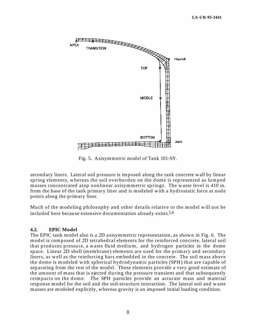
4.1. ABAQUS ModelThe ABAQUS tank model is shown in Fig. 5 and depicts a two-dimensional (2D)axisymmetric representation of the structure. The model is composed of 2D solidelements representing the reinforced concrete shell and dome and axisymmetric shellelements, which include membrane and bending for the primary and
LA-UR-95-3441
8
Fig. 5. Axisymmetric model of Tank 101-SY.
secondary liners. Lateral soil pressure is imposed along the tank concrete wall by linearspring elements, whereas the soil overburden on the dome is represented as lumpedmasses concentrated atop nonlinear axisymmetric springs. The waste level is 410 in.from the base of the tank primary liner and is modeled with a hydrostatic force at nodepoints along the primary liner.
Much of the modeling philosophy and other details relative to the model will not beincluded here because extensive documentation already exists.5,6
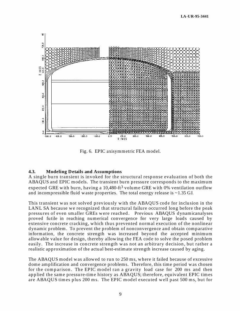
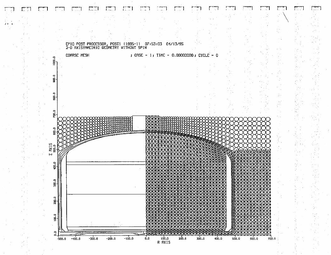
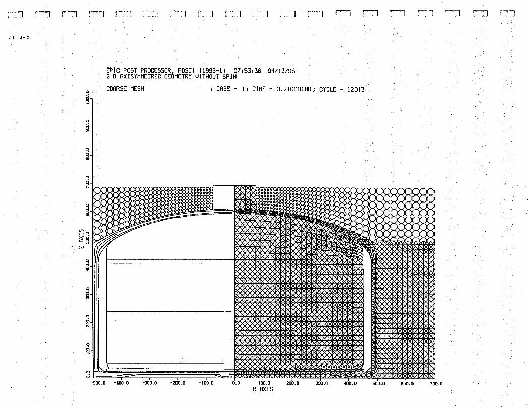
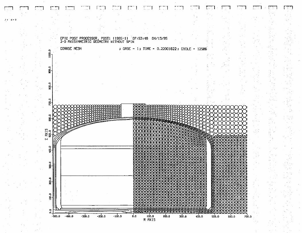
4.2. EPIC ModelThe EPIC tank model also is a 2D axisymmetric representation, as shown in Fig. 6. Themodel is composed of 2D tetrahedral elements for the reinforced concrete, lateral soilthat produces pressure, a waste fluid medium, and hydrogen particles in the domespace. Linear 2D shell (membrane) elements are used for the primary and secondaryliners, as well as the reinforcing bars embedded in the concrete. The soil mass abovethe dome is modeled with spherical hydrodynamic particles (SPH) that are capable ofseparating from the rest of the model. These elements provide a very good estimate ofthe amount of mass that is ejected during the pressure transient and that subsequentlyreimpacts on the dome. The SPH particles provide an accurate mass and materialresponse model for the soil and the soil-structure interaction. The lateral soil and wastemasses are modeled explicitly, whereas gravity is an imposed initial loading condition.
LA-UR-95-3441
9
Fig. 6. EPIC axisymmetric FEA model.
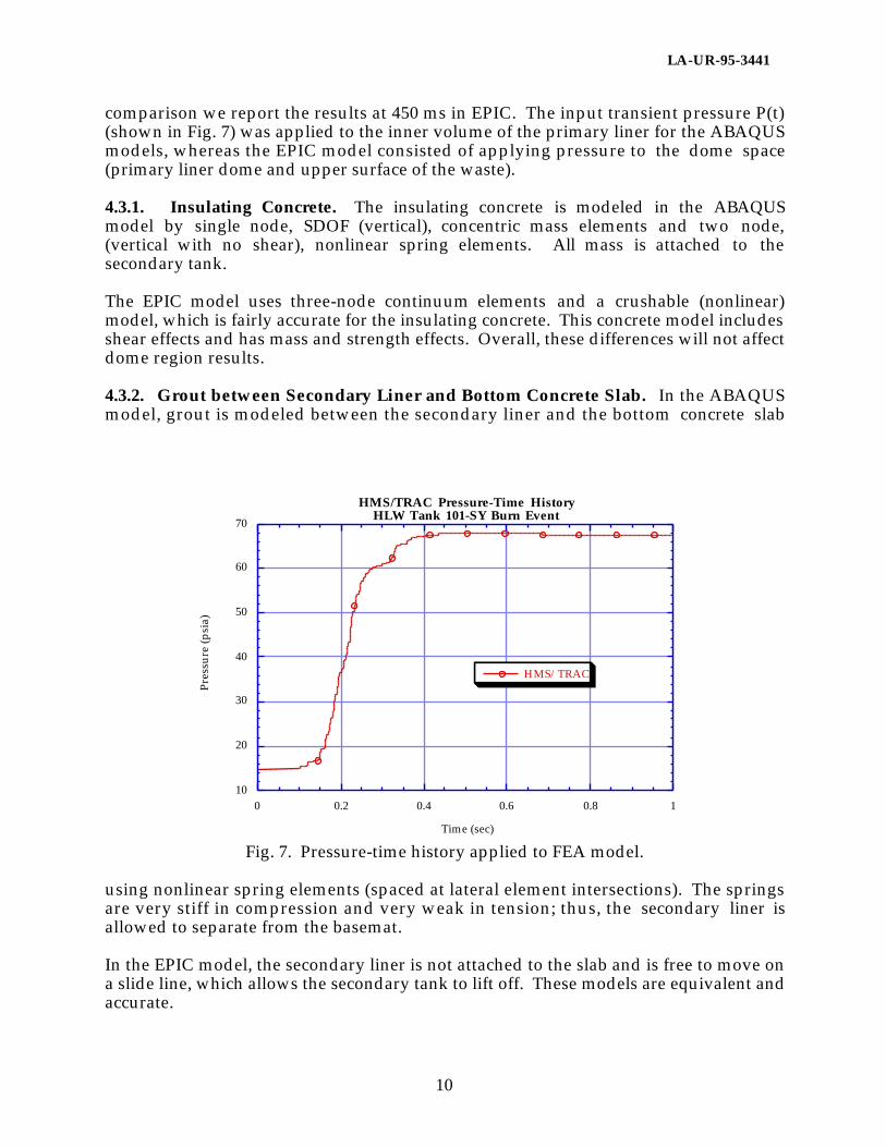
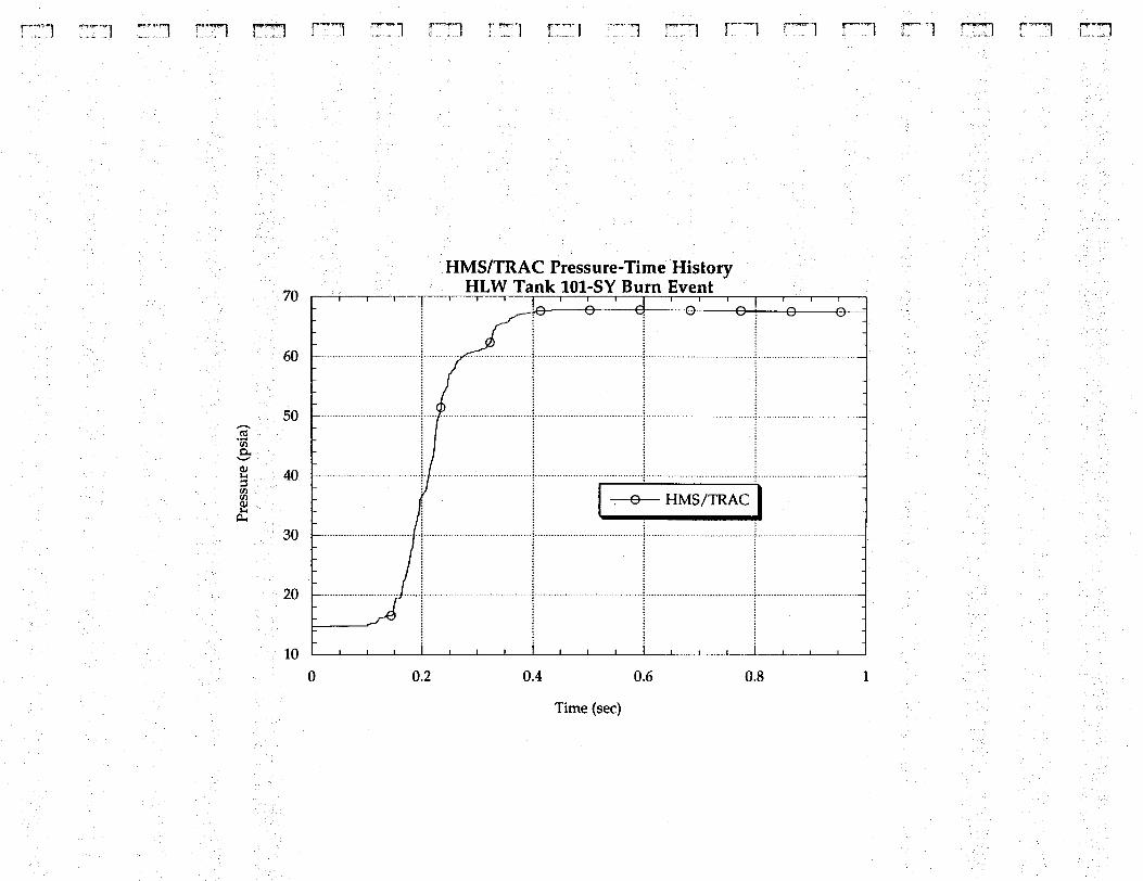
4.3. Modeling Details and AssumptionsA single burn transient is invoked for the structural response evaluation of both theABAQUS and EPIC models. The transient burn pressure corresponds to the maximumexpected GRE with burn, having a 10,480-ft3 volume GRE with 0% ventilation outflowand incompressible fluid waste properties. The total energy release is ~1.35 GJ.
This transient was not solved previously with the ABAQUS code for inclusion in theLANL SA because we recognized that structural failure occurred long before the peakpressures of even smaller GREs were reached. Previous ABAQUS dynamicanalysesproved futile in reaching numerical convergence for very large loads caused byextensive concrete cracking, which thus prevented normal execution of the nonlineardynamic problem. To prevent the problem of nonconvergence and obtain comparativeinformation, the concrete strength was increased beyond the accepted minimumallowable value for design, thereby allowing the FEA code to solve the posed problemeasily. The increase in concrete strength was not an arbitrary decision, but rather arealistic approximation of the actual best-estimate strength increase caused by aging.
The ABAQUS model was allowed to run to 250 ms, where it failed because of excessivedome amplification and convergence problems. Therefore, this time period was chosenfor the comparison. The EPIC model ran a gravity load case for 200 ms and thenapplied the same pressure-time history as ABAQUS; therefore, equivalent EPIC timesare ABAQUS times plus 200 ms. The EPIC model executed well past 500 ms, but for
LA-UR-95-3441
10
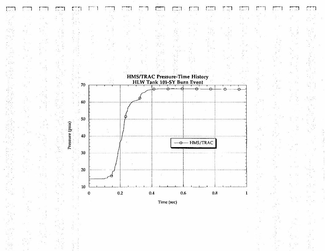
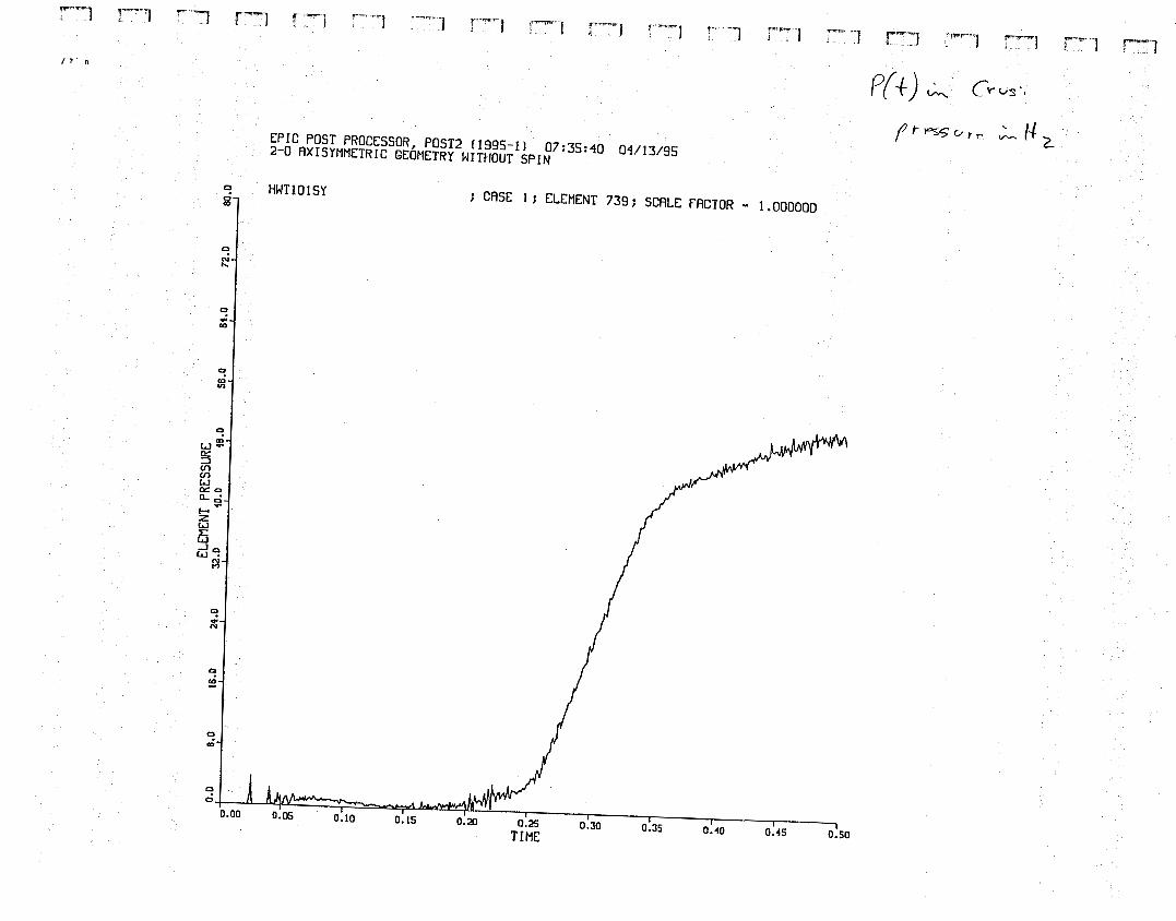
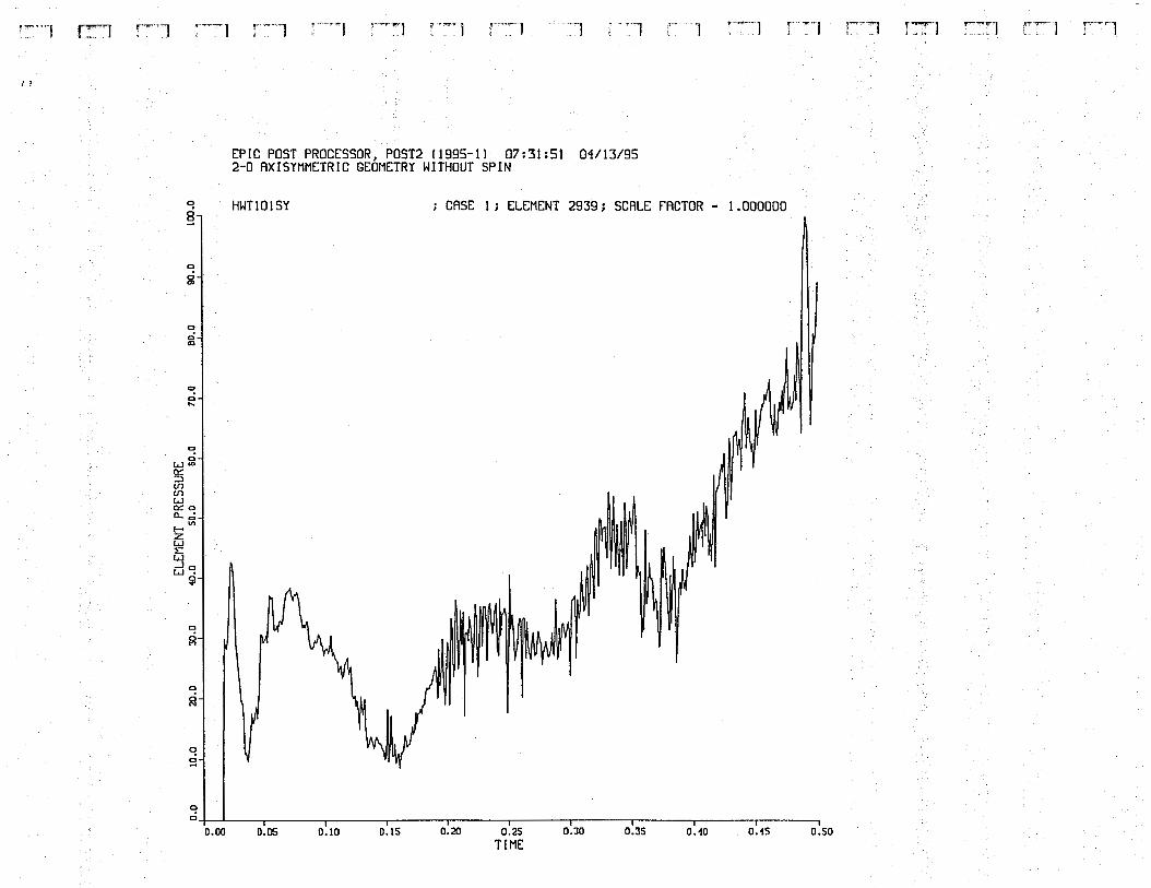
comparison we report the results at 450 ms in EPIC. The input transient pressure P(t)(shown in Fig. 7) was applied to the inner volume of the primary liner for the ABAQUSmodels, whereas the EPIC model consisted of applying pressure to the dome space(primary liner dome and upper surface of the waste).
4.3.1. Insulating Concrete. The insulating concrete is modeled in the ABAQUSmodel by single node, SDOF (vertical), concentric mass elements and two node,(vertical with no shear), nonlinear spring elements. All mass is attached to thesecondary tank.
The EPIC model uses three-node continuum elements and a crushable (nonlinear)model, which is fairly accurate for the insulating concrete. This concrete model includesshear effects and has mass and strength effects. Overall, these differences will not affectdome region results.
4.3.2. Grout between Secondary Liner and Bottom Concrete Slab. In the ABAQUSmodel, grout is modeled between the secondary liner and the bottom concrete slab
10
20
30
40
50
60
70
0 0.2 0.4 0.6 0.8 1
HMS/TRAC Pressure-Time HistoryHLW Tank 101-SY Burn Event
HMS/TRAC
Pre
ssu
re (
psi
a)
Time (sec)
Fig. 7. Pressure-time history applied to FEA model.
using nonlinear spring elements (spaced at lateral element intersections). The springsare very stiff in compression and very weak in tension; thus, the secondary liner isallowed to separate from the basemat.
In the EPIC model, the secondary liner is not attached to the slab and is free to move ona slide line, which allows the secondary tank to lift off. These models are equivalent andaccurate.
LA-UR-95-3441
11
4.3.3. Pump Pit and Soil above Dome. In the ABAQUS model, the pump pit and soilare represented as concentrated masses on the dome and remain attached to the domethroughout the analysis. This is not correct because the soil will separate from thedome if a large dynamic pressure pulse occurs.
In the EPIC model, the pump pit is modeled with continuum elements that are notattached to the dome top and therefore are able to separate. The soil above the dome ismodeled with SPH particles, which can displace during the transient. The pump pit andsoil therefore are modeled explicitly with elements and appropriate material models.
If the dome velocity is increasing upward, the models are considered to be equivalent.However, as the dome velocity slows down, the models are not equivalent and acomparison cannot be made.
4.3.4. Wastes. In the ABAQUS model, wastes are modeled with concentrated masselements attached to the sides and bottom of the primary liner, assuming variabledensity, as shown in Table 1 and described in Sec. 5.0. This corresponds to an averagedensity of = 1.60. These mass elements represent SDOF lumped masses that are uni-directional (radial on the side of the tank and vertical on the bottom). Two cases werestudied where (1) approximately half of the total waste mass was assumed to beactively participating radially with the primary liner (results shown in App. F), and (2)zero mass was assumed to be actively participating radially. The results for zero wasteparticipation are a closer approximation in agreement with the EPIC results.
TABLE 1
LIQUID WASTE CHARACTERISTICS
Material Specific Gravity DepthSlurry 1.71 0.7 m (18 in.)Slurry 1.66 4.3 m (172 in.)
C Layer 1.54 5.3 m (210 in.)
In the EPIC model, four distnct layers of waste are modeled using the appropriatedensities for the sludge, a nonconvecting layer, a convecting layer, and a crust. Allwastes are modeled as fluids that have no crushing and no tensile strength. Thecomposite waste layers represent an average density of = 1.63.
Overall, there is sufficient similarity between the models for this comparison. We foundthat fluid/structure interaction included in the EPIC model gave a radial velocity of theprimary liner that was significantly different from that given by theconservative mass representation in ABAQUS with half the radial mass. Although thismodeling assumption resulted in differences with meridional strains in the primaryliner, it did not have a significant effect with the dome motion.
LA-UR-95-3441
12
4.3.5. Hydrogen Burn. The hydrogen burn in the ABAQUS model is representedusing data from a time, pressure, and dome volume matrix and is calculated with theHMS/TRAC gas dynamics/chemical kinetics code. The pressure is assumed to beuniform throughout the primary tank (i.e., no spatial variation).
Hydrogen is represented by continuum elements in the EPIC model that completelyenclose the dome space volume. The detonation model is based on the volume,density, energy, and detonation velocity and location. To approximate the uniformpressure used in the ABAQUS model, we do not use the detonation model in EPIC.Rather, the pressure-time history of Fig. 7 is applied to the boundary of the hydrogenelements in the dome, whereas the lower wall of the tank achieves pressurization later.
There are differences in the models; however, the EPIC model was adjusted to providea condition to the ABAQUS model that was as similar as possible. These differences didnot appear to have a large effect on dome motion.
4.3.6. Rebar
4.3.6.1. Material models. In ABAQUS, rebar is modeled with concrete using acomposite material model.
In EPIC, rebar is modeled separately from concrete. The rebar is modeled as a thinmembrane using shell elements having no bending capability. The concrete is modeledwith separate (attached) continuum elements.
4.3.6.2. Radial (meridional) and circumferential (hoop) rebar. In the ABAQUS model,the radial (meridional) and circumferential (hoop) rebar are modeled separately, basedon thicknesses specified in the drawings for each location.
In the EPIC model, the radial and circumferential rebar in each element are modeled asa single-shell membrane element, with the thickness of the element based on anaverage of the thicknesses of the radial and circumferential rebar specified by thedrawings for each location. This smearing of circumferential and meridional rebar isnecessary because EPIC does not have an orthotropic or anisotropic material model.The variation between the meridional (radial) and circumferential (hoop) steel thereforecannot be modeled. In the dome region, this difference resulted in very small errors.In the basemat region, the errors were large. However, because the dome is the mostimportant portion of the tank structure under an internal pressurization event, this wasconsidered accurate enough for comparison.
In the dome and haunch area, the amount of rebar used in each model was in closeagreement (~10%) for important load-carrying rebar.
4.3.6.3. Distance between the rebar in the two faces of the concrete. In the ABAQUSmodel, the rebar is modeled 3 in. from the exterior face and 2.5 in. from the interior faceof the 15-in.-thick dome, which is a distance apart of 9.5 in. This probably is close to theas-built (as-constructed vs as-designed) case, which specifies a minimum 2-in. cover.
LA-UR-95-3441
13
The location (distance from faces and distance apart) in the EPIC model of mainreinforcing steel is not as accurate. The rebar is located 3.75 in. from each face, which isa distance of 7.5 in. apart.
Because of this difference in spacing, the bending stiffness of the steel alone in theABAQUS model is twice that in the EPIC model. Adjusting the steel to get the bendingstiffness correct would cause an error in the membrane stiffness, and both themembrane and the bending are important for this problem. However, the difference incomposite (steel and concrete)-section bending stiffness at ultimate capacity is only ~5%,with the EPIC model again being softer. The difference in the membrane stiffness isvery small. Because the dome’s concrete structure is representative of a semi-ellipticalshell, the major stresses will be on the membrane. Therefore, the comparison shouldbe quite close.
4.3.6.4. Shear steel. The shear steel is not modeled in either ABAQUS or EPIC. This isconsidered acceptable when the dome, or other concrete, reacts to the applied loads inthe membrane. However, it is not correct (or actually underpredicts thestrength/stiffness) when the dome or other components are in bending. PreviousABAQUS analyses have shown that the dome acts as a membrane, with little bendingfor uniform pressurization, as is assumed for this comparison (except in the upper-knuckle region). The shear steel should be included for modeling a spatially varyingburn or detonation (or the nonuniform impact of the pump pit and soil) because thedome and other components will be in a state of bending. Leaving out the shear steelwill underpredict the strength of the dome and therefore overpredict the consequences.The ABAQUS concrete model includes the capability to model the shear steel correctly.However, because the shear steel caused a numerical instability (ringing) as theconcrete reached failure, it was removed from the model for subsequent analyses.
The problem with modeling shear steel in EPIC is the lack of orthotropic or anisotropicmaterial models. Modeling the shear steel with membrane elements would add tocircumferential steel, which already is modeled with main reinforcing membraneelements. EPIC requires an orthotropic model to decouple the “through-thickness”strength/stiffness from the “radial-meridional” strength/stiffness. Because such amodel is not available in EPIC, leaving out the shear steel and the resultingoverprediction of damage and consequences was the best alternative and wasconsidered a conservative estimate.
4.3.6.5. Overall rebar assessment. The bending and membrane stiffness/strength ofthe dome and haunch region are modeled accurately enough in EPIC for the burn (ordetonation) and the pump and soil reimpaction case. This is true especially for theABAQUS/EPIC comparison, where the load is spatially uniform.
4.3.7. Soil. The ABAQUS model uses unidirectional interface elements to model thesoil around the sides and bottom of the tank. These elements are similar tounidirectional gap elements with a linear spring stiffness and frictional effect normal tothe gap. The ABAQUS model assumes that the soil is isotropic and uses an expectedlateral earth pressure, based on the soil properties, to calculate the spring stiffness andapplied loads required to resist the motion of the tank.
LA-UR-95-3441
14
The EPIC model uses continuum and SPH particles to model the soil, with soakerelements near the boundaries of the model around the sides and bottom of the tank.This model has ~25 ft of soil around the tank. The soaker elements absorb stress wavesand make the soil act as an “infinite medium.” The soil is modeled as a crushablematerial that predicts sand behavior accurately, including nonlinear crushing. The soilfriction on the concrete tank wall was modeled with slide lines using the same value asin the ABAQUS model (0.57). This high value of friction was found previously6 tominimize tank damage. The EPIC model includes a very accurate representation of thesoil/structure interaction effects.
Overall, if the concrete wall does not move much into the soil, then modelingdifferences will be small. For larger concrete wall motion, the EPIC soil model willabsorb more energy than the ABAQUS model.
4.3.8. Waste Compressibility. The pressure transient input to ABAQUS is based onthe HMS/TRAC gas dynamics code and assumes an incompressible waste. In the EPICmodel, waste is modeled with H2O stiffness (incompressible at low pressure). Thesemodeling philosophies will give essentially the same results for the comparisoncalculation.
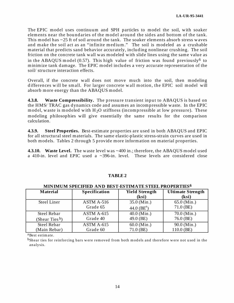
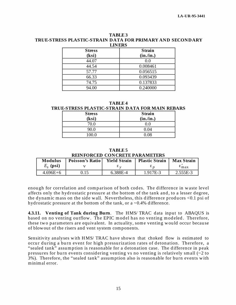
4.3.9. Steel Properties. Best-estimate properties are used in both ABAQUS and EPICfor all structural steel materials. The same elastic-plastic stress-strain curves are used inboth models. Tables 2 through 5 provide more information on material properties.
4.3.10. Waste Level. The waste level was ~400 in.; therefore, the ABAQUS model useda 410-in. level and EPIC used a ~396-in. level. These levels are considered close
TABLE 2
MINIMUM SPECIFIED AND BEST-ESTIMATE STEEL PROPERTIES6
Material Specification Yield Strength(ksi)
Ultimate Strength(ksi)
Steel Liner ASTM A-516Grade 65
35.0 (Min.)44.0 (BEa)
65.0 (Min.)71.0 (BE)
Steel Rebar(Shear Ties b)
ASTM A-615Grade 40
40.0 (Min.)49.0 (BE)
70.0 (Min.)76.0 (BE)
Steel Rebar(Main Rebar)
ASTM A-615Grade 60
60.0 (Min.)71.0 (BE)
90.0 (Min.)110.0 (BE)
aBest estimate.bShear ties for reinforcing bars were removed from both models and therefore were not used in theanalysis.
LA-UR-95-3441
15
TABLE 3TRUE-STRESS PLASTIC-STRAIN DATA FOR PRIMARY AND SECONDARY
LINERSStress(ksi)
Strain(in./in.)
44.07 0.044.54 0.00846157.77 0.05651566.33 0.09343974.75 0.13783394.00 0.240000
TABLE 4TRUE-STRESS PLASTIC-STRAIN DATA FOR MAIN REBARS
Stress(ksi)
Strain(in./in.)
70.0 0.090.0 0.04100.0 0.08
TABLE 5REINFORCED CONCRETE PARAMETERS
Modulus
Es (psi)Poisson’s Ratio Yield Strain
y
Plastic Strain
p
Max Strain
′ max
4.696E+6 0.15 6.388E-4 1.917E-3 2.555E-3
enough for correlation and comparison of both codes. The difference in waste levelaffects only the hydrostatic pressure at the bottom of the tank and, to a lesser degree,the dynamic mass on the side wall. Nevertheless, this difference produces <0.1 psi ofhydrostatic pressure at the bottom of the tank, or a ~0.4% difference.
4.3.11. Venting of Tank during Burn. The HMS/TRAC data input to ABAQUS isbased on no venting outflow. The EPIC model has no venting modeled. Therefore,these two parameters are equivalent. In actuality, some venting would occur becauseof blowout of the risers and vent system components.
Sensitivity analyses with HMS/TRAC have shown that choked flow is estimated tooccur during a burn event for high pressurization rates of detonation. Therefore, a“sealed tank” assumption is reasonable for a detonation case. The difference in peakpressures for burn events considering venting vs no venting is relatively small (~2 to3%). Therefore, the “sealed tank” assumption also is reasonable for burn events withminimal error.
LA-UR-95-3441
16
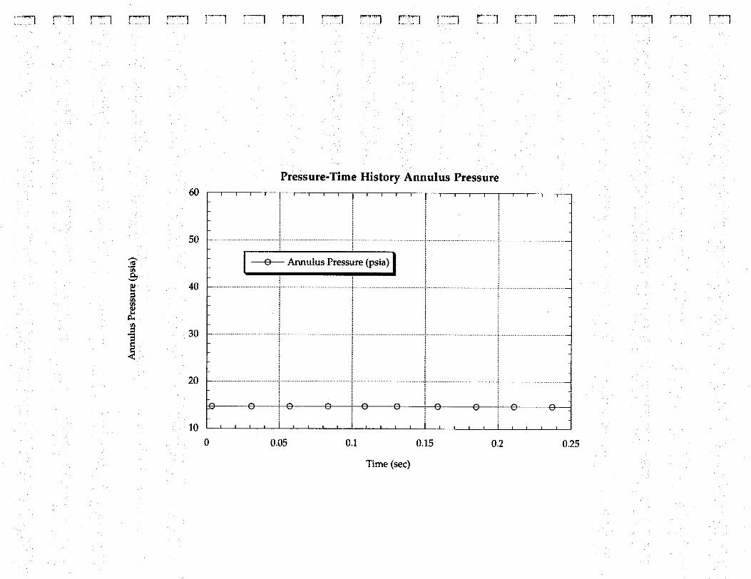
4.3.12. Annulus Air Pressure. If the annulus were sealed, the entrained air wouldresist radial motion of the primary tank. Previous ABAQUS models used an annulusspring equivalent to the Ideal Gas Law. Because the annulus is vented to theatmosphere, it is not assumed to be sealed; therefore, no resistance to radial growth isexpected. Also, the EPIC model does not have an air spring model for the annulus.Thus, the air spring was removed from the ABAQUS model for the comparisoncalculation.
4.3.13. Rebar Debonding. In ABAQUS, a rebar reaching ultimate strength debondsfrom the concrete and subsequently is removed from the problem. It is replaced with anew stiffness matrix that is based solely on concrete.
In the EPIC model, the rebar fractures at an ultimate strain of 8% and no longer cancarry tensile loads. Furthermore, the rebar is removed from the problem when theplastic strains exceed 60%. These models are similar enough to be comparable.
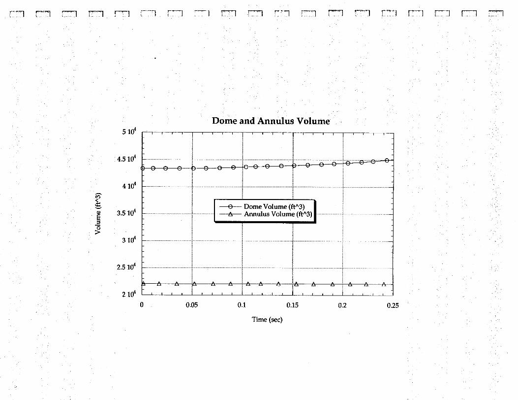
4.3.14. Initial Dome Volume. An initial dome volume of 43,300 ft3 before burn eventinitiation is the same in both models.
4.3.15. Concrete Modeling. The concrete algorithm in ABAQUS is based on definingits compressive properties outside the elastic regime, although linear elasticity stillapplies within approximately one-half of the compressive strength. This is applied bydefining a compressive stress as a function of plastic strain. The model further includes(1) shear retention, which defines the modulus for shearing of cracks such that thismodel assumes that the shear stiffness of open cracks reduces linearly to zero as thecrack opening increases; (2) tension stiffening, which defines the retained tensile stressnormal to a crack, is used primarily to allow some effect of interaction between thereinforcing bars and concrete and allow a smearing of cracking over a finite volume;and (3) failure ratios, which define the shape of the failure surface based on biaxialityeffects. Cracking dominates the material behavior when the state of stresspredominantly is tensile. The model uses a “crack detection” plasticity surface at eachintegration point to determine when cracking takes place. Subsequent to the crackdetection increment, a damaged elasticity model is implemented. Rebar elements areembedded within the oriented surfaces of the concrete element.
The EPIC concrete model uses the Holmquist-Johnson-Cook (H-J-C) concrete strengthmodel that includes the Mie-Gruneisen (M-G) equation of state (EOS) (see Fig. 8 in Sec. 5on Material Properties). Both models used the same compressive strength andconcrete-specific models. These EPIC models are considered sufficiently similar toABAQUS models to make this comparison with negligible error.
4.3.16. Gravity. ABAQUS and EPIC models both include gravity as an initialpreloading state of the structures. ABAQUS solves static gravity load (exactly) over sixtimesteps to allow minor deviations of nonlinearities to settle and is applied before theburn pressure.
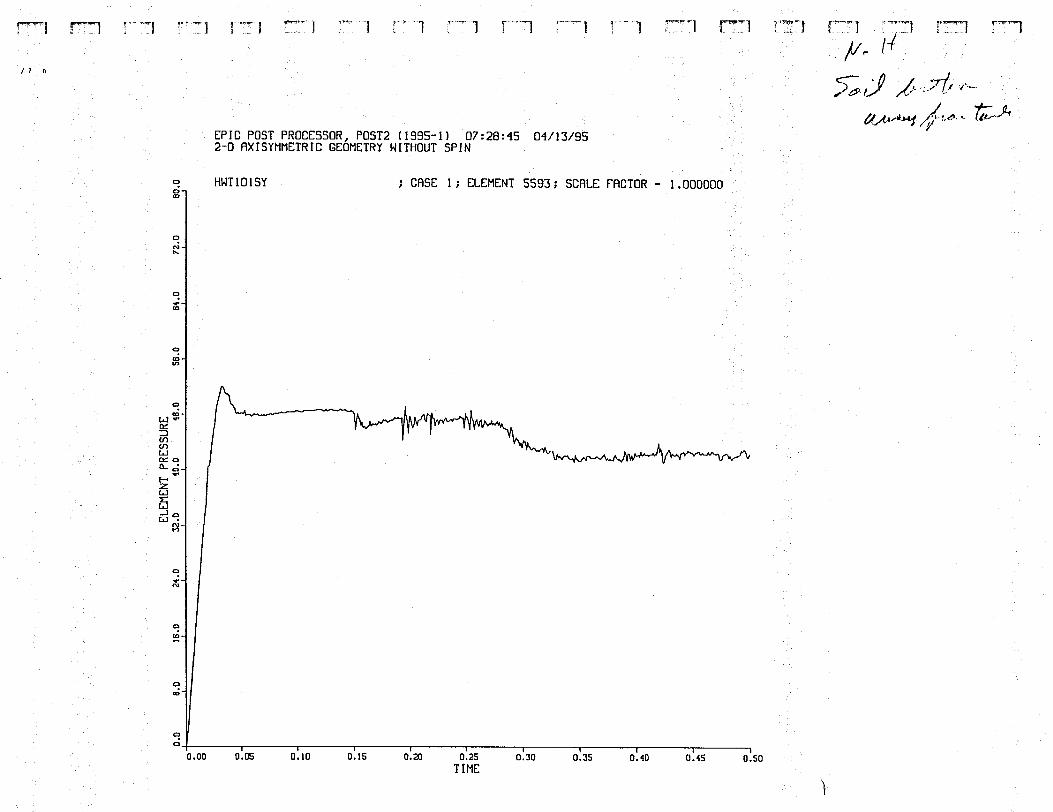
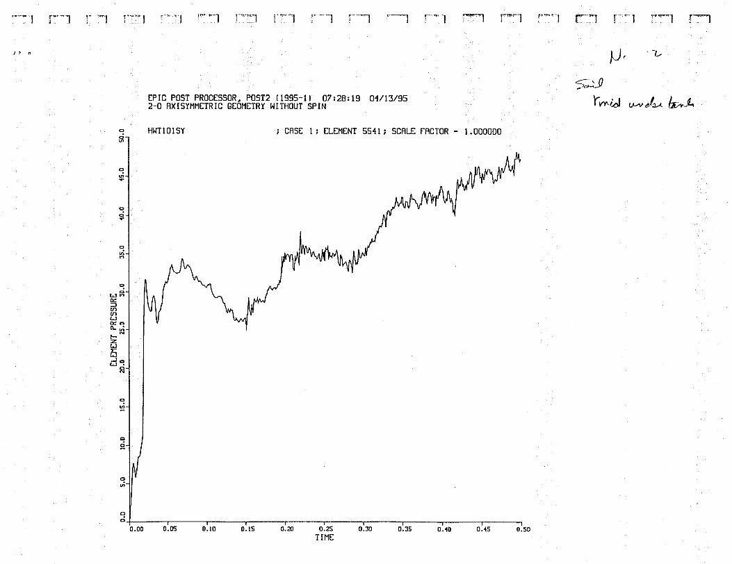
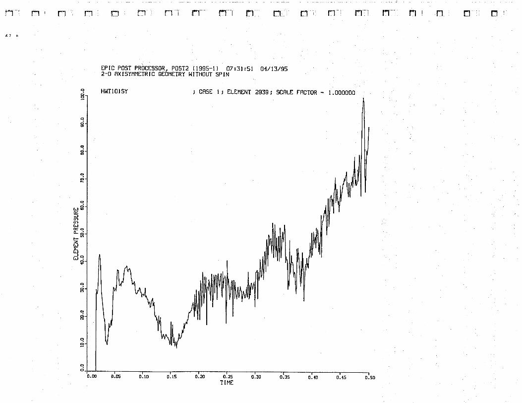
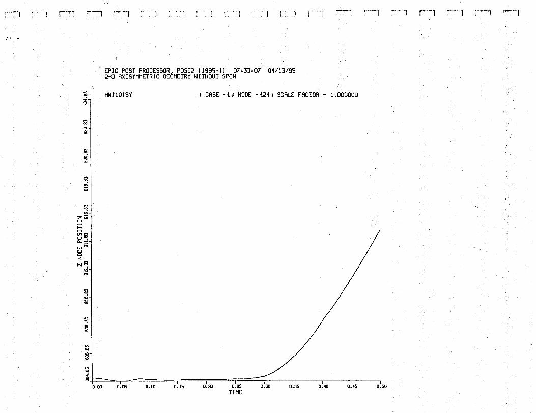
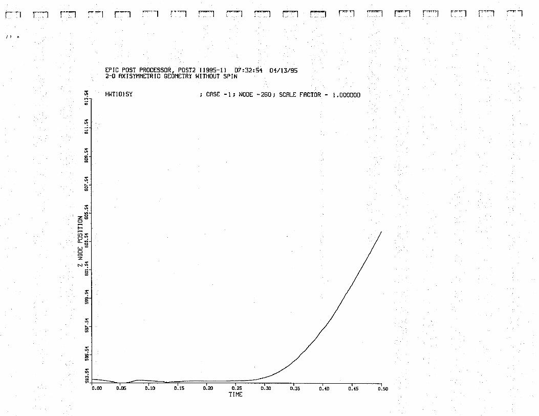
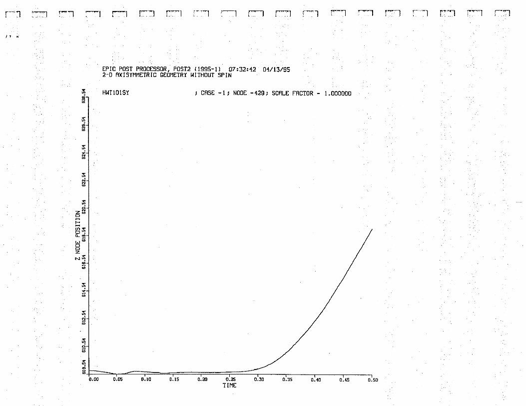
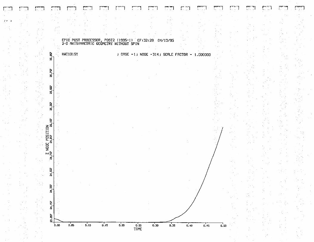
EPIC was executed until the gravity load was “approximately right”; then the pressure-time history was applied. This procedure is not exact because we did not run EPIC untilall dynamic wave oscillations had settled out [see soil P(t) curves at the bottom of
LA-UR-95-3441
17
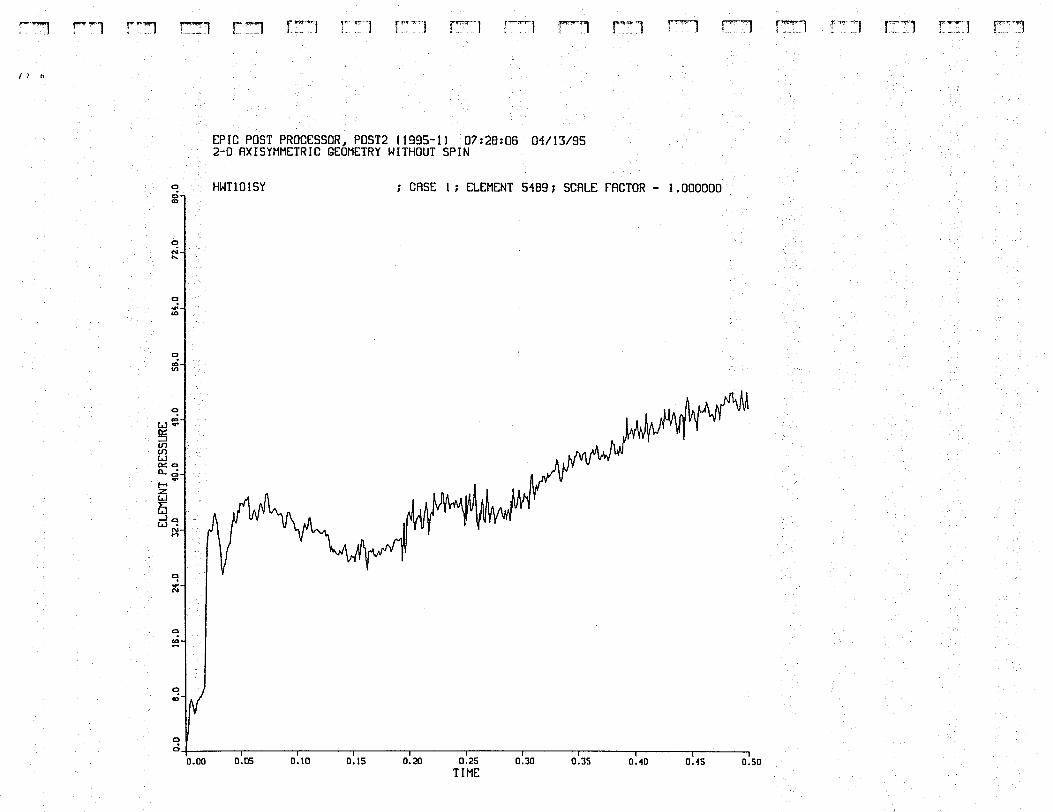
element No. 5541 as a good example of these oscillations (App. B)]. This procedureshows the pressure caused by gravity out to 200 ms; the pressure from the burn then isadded. Element No. 5593 was not under the tank and shows only the 47-psi soilpressure. Comparing this to 47 psi gives the accuracy of this approximation in EPIC.This approximation is considered to incur negligible error.
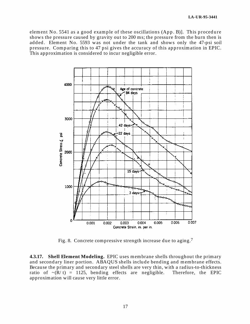
Fig. 8. Concrete compressive strength increase due to aging.7
4.3.17. Shell Element Modeling. EPIC uses membrane shells throughout the primaryand secondary liner portion. ABAQUS shells include bending and membrane effects.Because the primary and secondary steel shells are very thin, with a radius-to-thicknessratio of ~(R/t) = 1125, bending effects are negligible. Therefore, the EPICapproximation will cause very little error.
LA-UR-95-3441
18
4.3.18. Air Chamber Drain Hole. A drain/vent space (hole) between the primary andsecondary liners of the tank and centrally located at the bottom is modeled correctly asan open space by ABAQUS. EPIC approximated the vent space with continuumelements that hypothetically were filled with polyurethane foam, thus providing notensile strength, very low density, and very low resistance to compression. Thisprocedure produces a bulk modulus of ~1 psi, which for our purposes is negligible.Therefore, these models are considered to be equivalent.
4.3.19. Failure Modeling
4.3.19.1. ABAQUS. As stated previously, the ABAQUS concrete failure modeling uses acrack detection surface for predominantly tensile principal stresses at each integrationpoint within the element. Because these are four-noded continuum elements, there arefour integration points at Gaussian locations that detect cracking. Therefore, only twocracks per integration point can be present in a 2D problem. However, because thepredominant tensile stress in an element is unidirectional, only four cracks will bepresent. As further element cracking continues, the model reduces to a damagedelasticity algorithm, where the element stiffness is reduced or no longer is used in thecalculations (i.e., zero concrete stiffness is assumed). Basically, the model employs acrack criterion that assumes zero stiffness (removed from stiffness matrix) when theelement has developed cracks at all four Gaussian integration points.
Rebar elements embedded within the concrete elements are “tied” to the isoparametriccoordinates. In 2D axisymmetric models, the rebar spacing is used to determine theoverall volume or modified rebar thickness. Material failure is implemented throughan elastic-plastic material model, where its true-stress true-strain relationship is definedup to its ultimate strength.
Primary and secondary liner failure model is derived through an isotropic elastic-plasticmaterial definition. No explicit failure was incorporated for steel.
4.3.19.2. EPIC. As mentioned previously, the EPIC concrete algorithm (H-J-C model)includes a fracture damage model to reduce strength and stiffness. In addition, whenthe concrete reaches 100% strain (based on volumetric strain or equivalent compressiveor shear/tension), the element is removed completely from the calculations. Theelement then attains zero stiffness, which is applied in the subsequent time increment.This is approximately equivalent to the cracking in the ABAQUS model.
Steel elements are modeled with the Johnson-Cook (J-C) elastic-plastic algorithm(similar to ABAQUS). In addition, at the appropriate failure strain (8% for rebar and24% for liner), the elements are removed from the model.
The minimum allowable tensile load (Pmin) was set to zero for the soil and all wastelayers, thereby forcing these materials to support zero tension. For the insulatingconcrete, the minimum allowable load was set to 5 psi, indicating a very low tensilestrength.
LA-UR-95-3441
19
4.3.20. Mesh Refinement. Mesh refinement of the steel liner and concrete wasconsidered similar for both the ABAQUS and EPIC nonlinear models. There were nomesh-sensitivity studies conducted with either models for optimizing the response ofthe structures. However, confirmatory-type evaluations of mesh size and mesh densityvs computer runtime for the ABAQUS nonlinear model have shown5 that its currentmodel is a best-estimate case.
We therefore conclude that both the ABAQUS and EPIC models are accurate enough toprovide a comparison.
5.0. MATERIAL PROPERTIES AND MODELS
5.1. WasteWaste fluid properties shown in Table 1 were used to calculate the overall mass on thebase of the tank, as well as to calculate the representation of dead weight andhydrostatic force on the primary liner. As stated previously, two cases were conductedwith the ABAQUS model, where the radial dynamic waste mass was varied from 0 to50%.
The original SA1 assumed a 50% radial mass in actively participating with the linerstructure. This was a best-guess estimate of the dynamic properties of waste fluid.
The ABAQUS model that was used to compare with the EPIC model implemented zeroradial waste mass actively participating dynamically. The properties of Table 1 wereused to model both the EPIC and ABAQUS models for dead-weight and hydrostaticeffects.
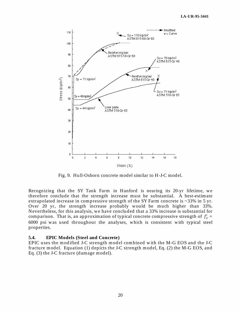
5.2. Steel LinersThe primary and secondary liners are manufactured from ASTM A-516 Gr 65, which is acommon pressure vessel steel in the US nuclear and fossil fuel industries. Table 2provides a listing of minimum material properties for the reinforcing steel and primaryand secondary shell. Engineering stress-strain data are shown in Fig. 9 for both theliner and rebar steels. These data are “nominal” material properties considered for abest-estimate safety analysis. However, actual true-stress-strain data were used for thenonlinear representation of these materials, as shown in Tables 3 and 4 for the ABAQUSmodel. The primary and secondary liner data show that the yield strength at 0% plasticstrain is ~44 ksi.
5.3. Concrete StrengthThe 28-day minimum compressive strength concrete was specified as the structuralmaterial for Tank 101-SY, with a minimum value of 4500 psi. As stated previously,because aging effects increase, the compressive strength of concrete was used for bothmodels. Aging effects increase the compressive strength dramatically over the initial 3to 6 months of curing (Fig. 8). Samples of concrete aggregates have shown8 a 5-yrstrength increase from 17 to 86% for different types of aggregates.
LA-UR-95-3441
20
Fig. 9. Hull-Osborn concrete model similar to H-J-C model.
Recognizing that the SY Tank Farm in Hanford is nearing its 20-yr lifetime, wetherefore conclude that the strength increase must be substantial. A best-estimateextrapolated increase in compressive strength of the SY Farm concrete is ~33% in 5 yr.Over 20 yr, the strength increase probably would be much higher than 33%.Nevertheless, for this analysis, we have concluded that a 33% increase is substantial forcomparison. That is, an approximation of typical concrete compressive strength of ′ f c =6000 psi was used throughout the analyses, which is consistent with typical steelproperties.
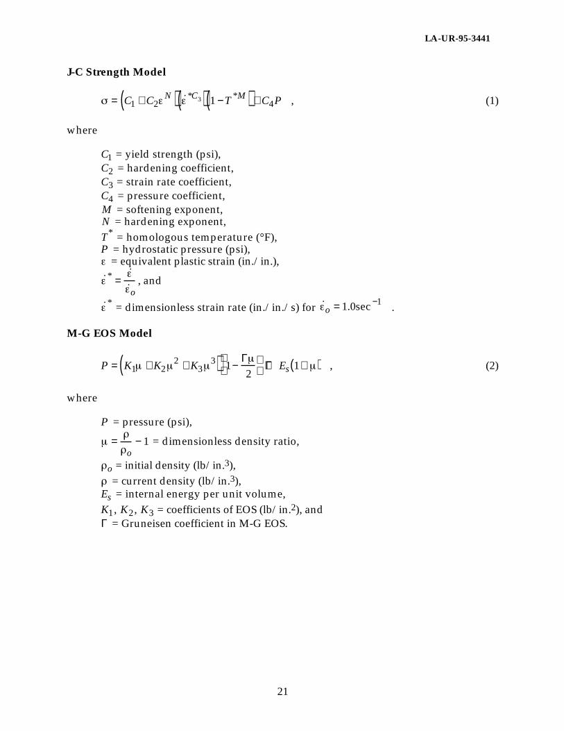
5.4. EPIC Models (Steel and Concrete)EPIC uses the modified J-C strength model combined with the M-G EOS and the J-Cfracture model. Equation (1) depicts the J-C strength model, Eq. (2) the M-G EOS, andEq. (3) the J-C fracture (damage model).
LA-UR-95-3441
21
J-C Strength Model
= C1 + C2
N( ) ˙ *C3( ) 1 −T *M( ) + C4P , (1)
where
C1 = yield strength (psi),
C2 = hardening coefficient,
C3 = strain rate coefficient,
C4 = pressure coefficient,
M = softening exponent, N = hardening exponent,
T* = homologous temperature (°F),
P = hydrostatic pressure (psi), = equivalent plastic strain (in./in.),
˙ * =
˙
˙ o, and
* = dimensionless strain rate (in./in./s) for
˙ o = 1.0sec −1 .
M-G EOS Model
P = K1 + K2
2 + K33( ) 1−
Γ2
+ΓEs 1+( ) , (2)
where
P = pressure (psi),
=
o− 1 = dimensionless density ratio,
o = initial density (lb/in.3),
= current density (lb/in.3),
Es = internal energy per unit volume,
K1 , K2 , K3 = coefficients of EOS (lb/in.2), andΓ = Gruneisen coefficient in M-G EOS.
LA-UR-95-3441
22
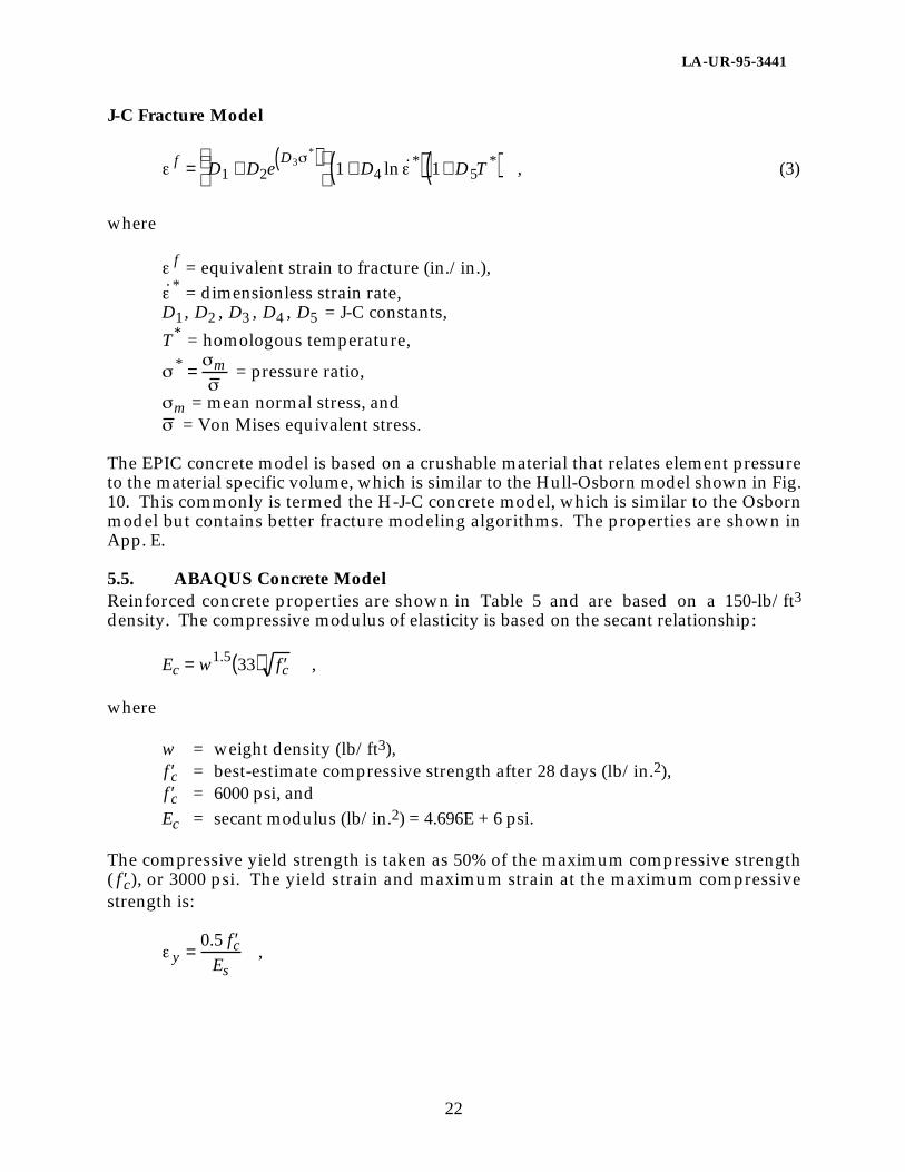
J-C Fracture Model
f = D1 + D2eD3
*( )
1 + D4 ln ˙ *( ) 1+ D5T
*( ) , (3)
where
f = equivalent strain to fracture (in./in.),
* = dimensionless strain rate,
D1 , D2 , D3 , D4 , D5 = J-C constants,
T* = homologous temperature,
* = m = pressure ratio,
m = mean normal stress, and = Von Mises equivalent stress.
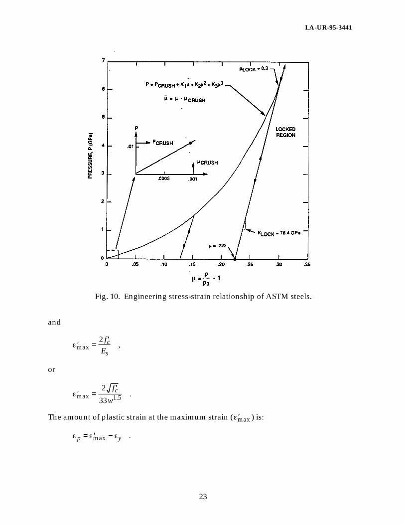
The EPIC concrete model is based on a crushable material that relates element pressureto the material specific volume, which is similar to the Hull-Osborn model shown in Fig.10. This commonly is termed the H-J-C concrete model, which is similar to the Osbornmodel but contains better fracture modeling algorithms. The properties are shown inApp. E.
5.5. ABAQUS Concrete ModelReinforced concrete properties are shown in Table 5 and are based on a 150-lb/ft3density. The compressive modulus of elasticity is based on the secant relationship:
Ec = w1.5 33( ) ′ f c ,
where
w = weight density (lb/ft3),
′ f c = best-estimate compressive strength after 28 days (lb/in.2),
′ f c = 6000 psi, and
Ec = secant modulus (lb/in.2) = 4.696E + 6 psi.
The compressive yield strength is taken as 50% of the maximum compressive strength( ′ f c), or 3000 psi. The yield strain and maximum strain at the maximum compressivestrength is:
y =
0.5 ′ f cEs
,
LA-UR-95-3441
23
Fig. 10. Engineering stress-strain relationship of ASTM steels.
and
′ max =
2 ′ f cEs
,
or
′ max =
2 ′ f c33w1.5 .
The amount of plastic strain at the maximum strain ( ′ max ) is:
p = ′ max − y .
LA-UR-95-3441
24
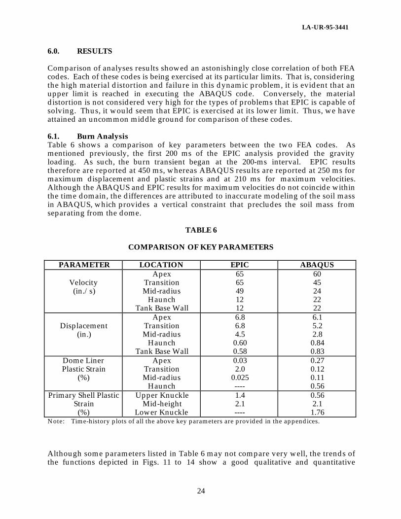
6.0. RESULTS
Comparison of analyses results showed an astonishingly close correlation of both FEAcodes. Each of these codes is being exercised at its particular limits. That is, consideringthe high material distortion and failure in this dynamic problem, it is evident that anupper limit is reached in executing the ABAQUS code. Conversely, the materialdistortion is not considered very high for the types of problems that EPIC is capable ofsolving. Thus, it would seem that EPIC is exercised at its lower limit. Thus, we haveattained an uncommon middle ground for comparison of these codes.
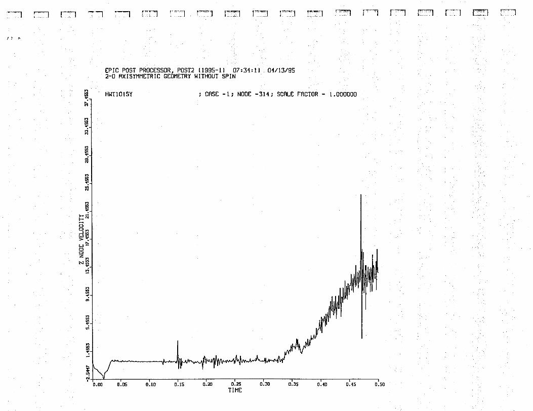
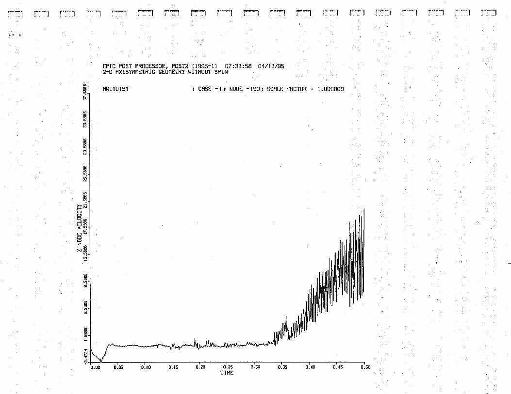
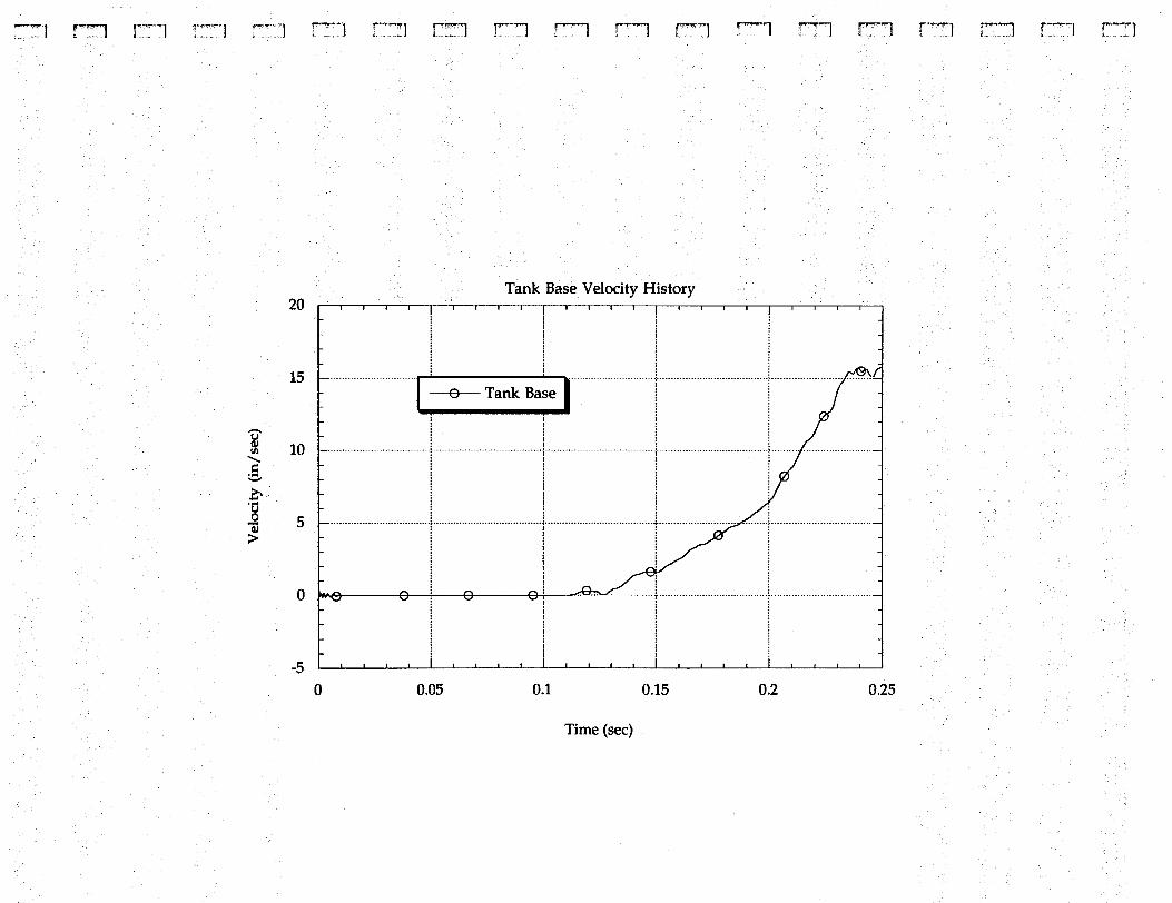
6.1. Burn AnalysisTable 6 shows a comparison of key parameters between the two FEA codes. Asmentioned previously, the first 200 ms of the EPIC analysis provided the gravityloading. As such, the burn transient began at the 200-ms interval. EPIC resultstherefore are reported at 450 ms, whereas ABAQUS results are reported at 250 ms formaximum displacement and plastic strains and at 210 ms for maximum velocities.Although the ABAQUS and EPIC results for maximum velocities do not coincide withinthe time domain, the differences are attributed to inaccurate modeling of the soil massin ABAQUS, which provides a vertical constraint that precludes the soil mass fromseparating from the dome.
TABLE 6
COMPARISON OF KEY PARAMETERS
PARAMETER LOCATION EPIC ABAQUS
Velocity(in./s)
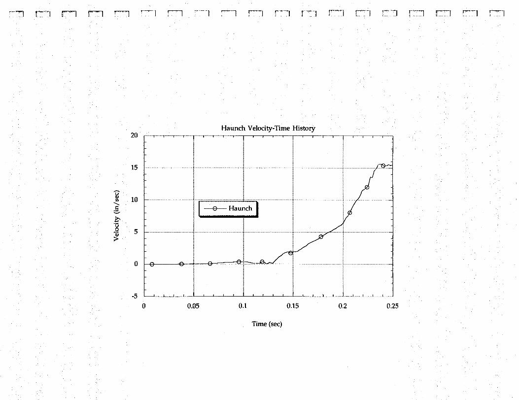
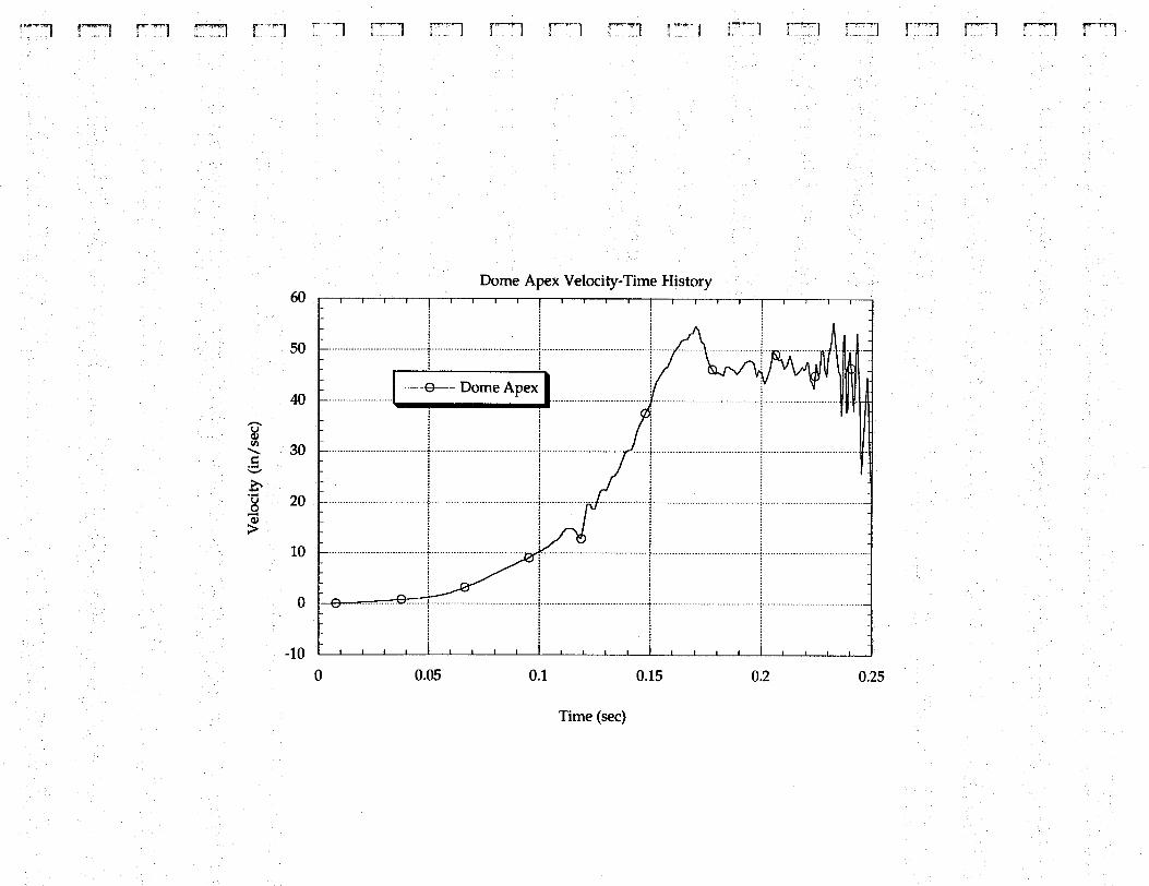
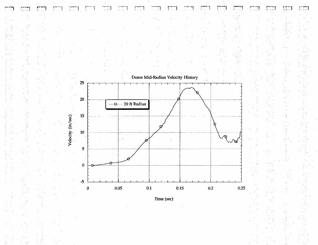
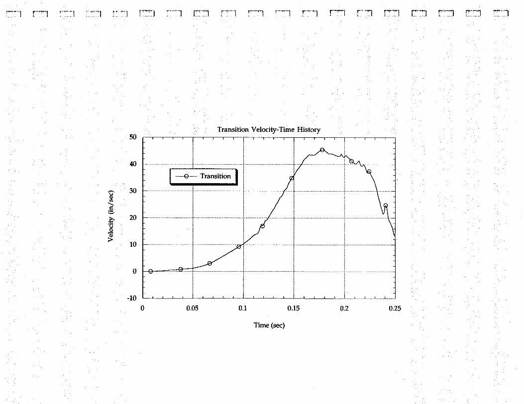
ApexTransitionMid-radius
HaunchTank Base Wall
6565491212
6045242222
Displacement(in.)
ApexTransitionMid-radius
HaunchTank Base Wall
6.86.84.50.600.58
6.15.22.80.840.83
Dome LinerPlastic Strain
(%)
ApexTransitionMid-radius
Haunch
0.032.0
0.025----
0.270.120.110.56
Primary Shell PlasticStrain(%)
Upper KnuckleMid-height
Lower Knuckle
1.42.1----
0.562.11.76
Note: Time-history plots of all the above key parameters are provided in the appendices.
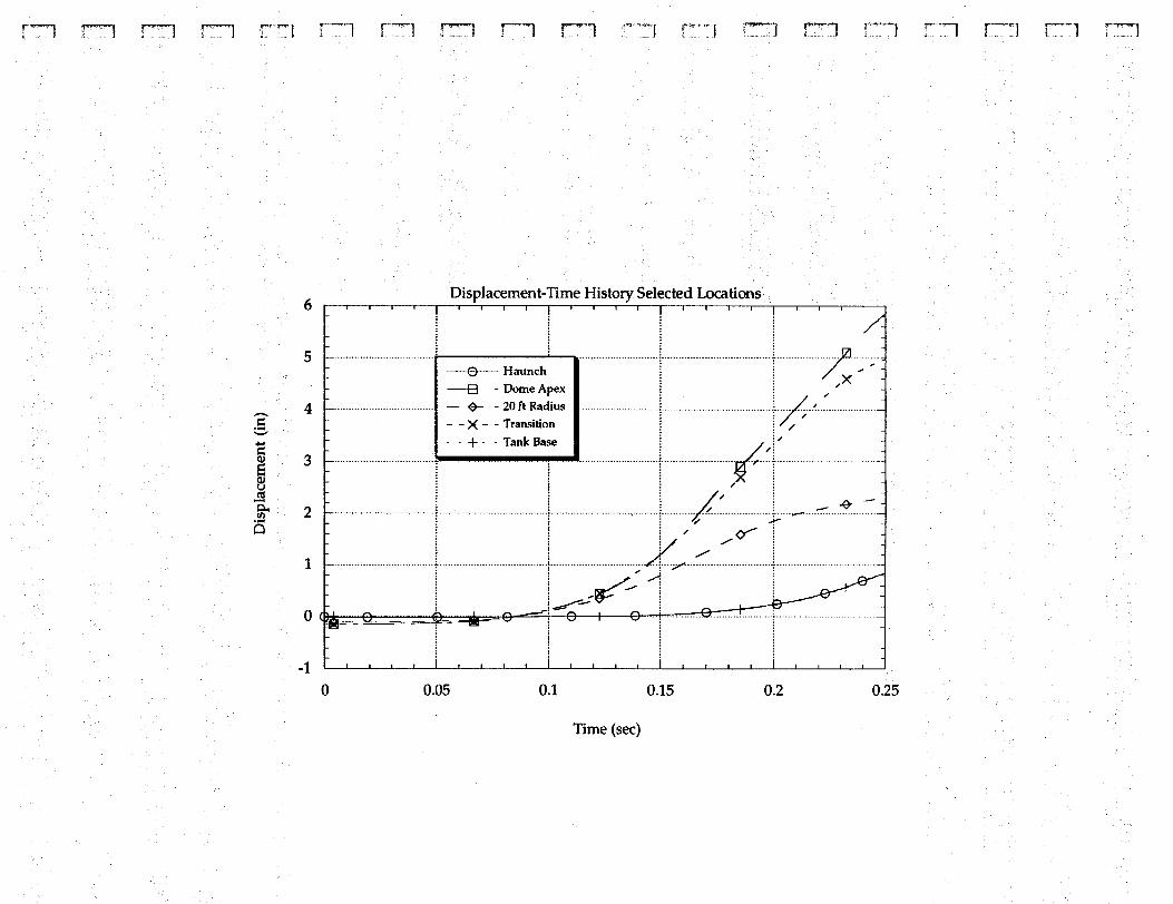
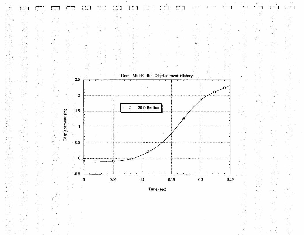
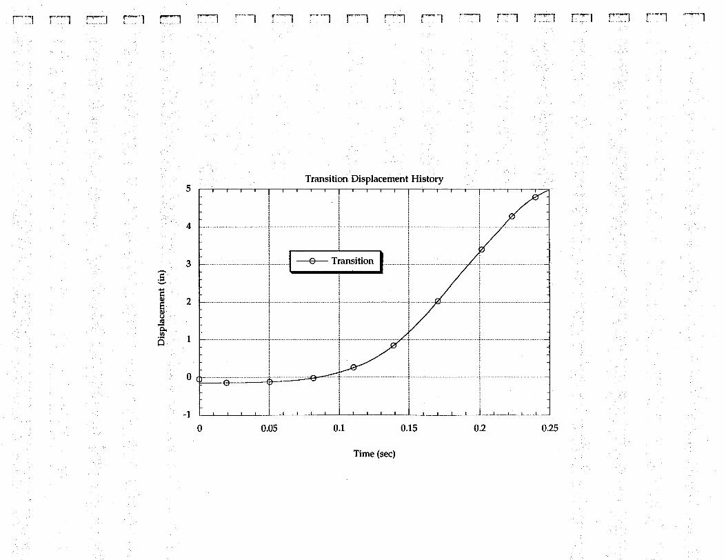
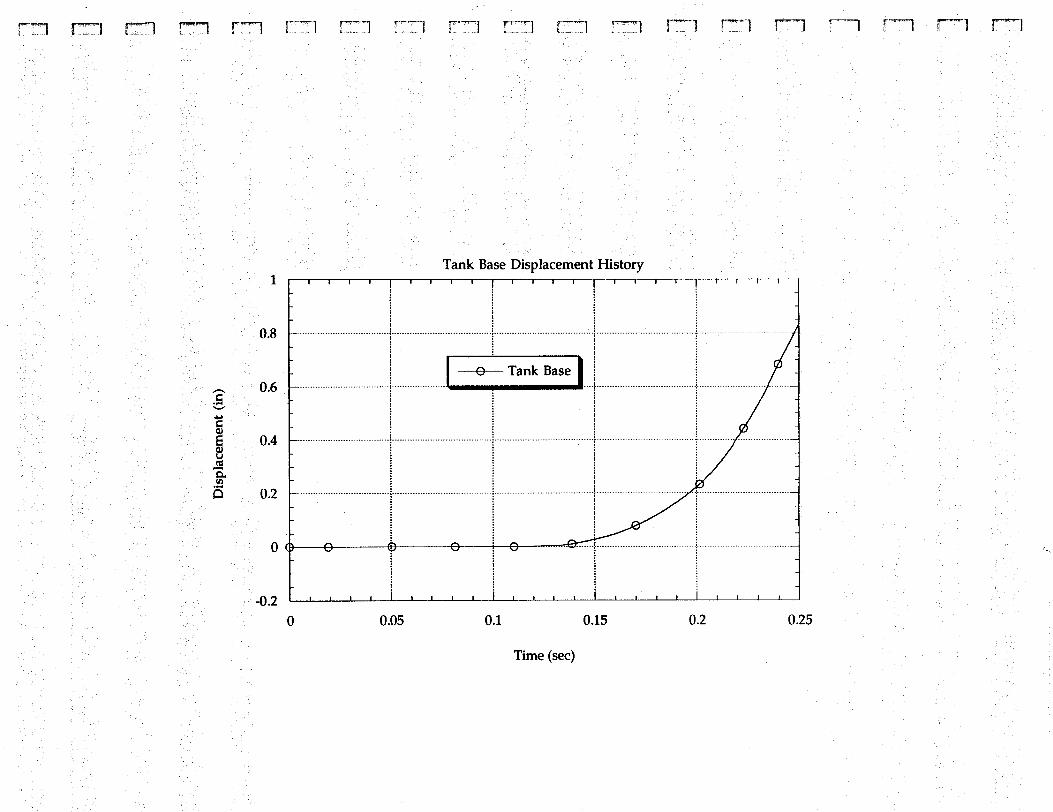
Although some parameters listed in Table 6 may not compare very well, the trends ofthe functions depicted in Figs. 11 to 14 show a good qualitative and quantitative
LA-UR-95-3441
25
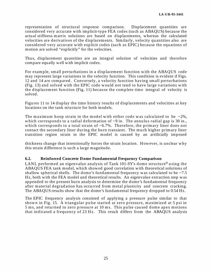
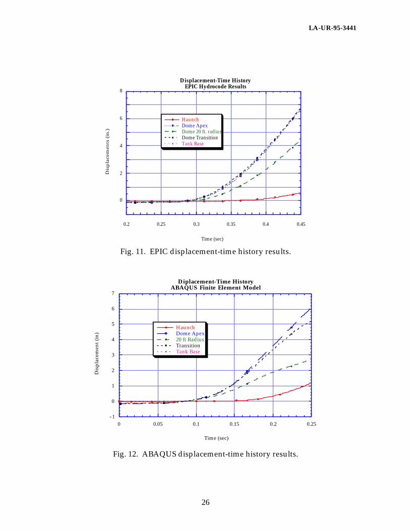
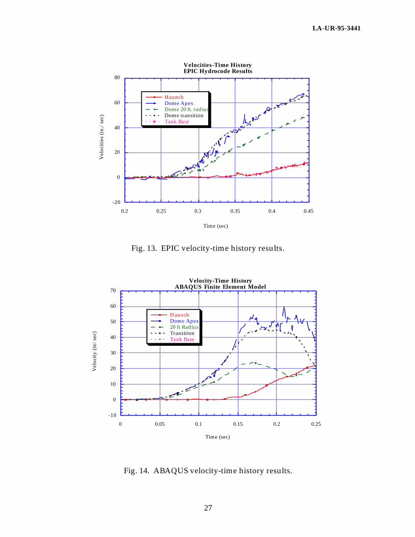
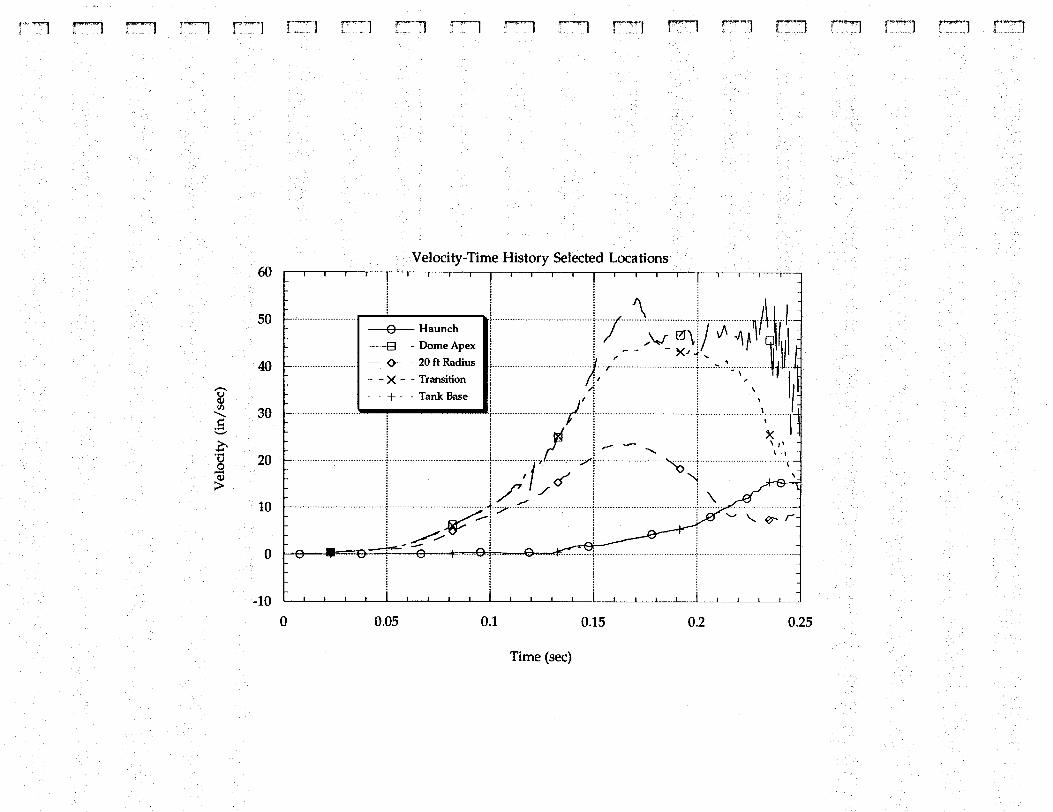
representation of structural response comparison. Displacement quantities areconsidered very accurate with implicit-type FEA codes (such as ABAQUS) because theactual stiffness matrix solutions are based on displacements, whereas the calculatedvelocities are derivatives of the displacements. Similarly, velocity quantities also areconsidered very accurate with explicit codes (such as EPIC) because the equations ofmotion are solved “explicitly” for the velocities.
Thus, displacement quantities are an integral solution of velocities and thereforecompare equally well with implicit codes.
For example, small perturbations in a displacement function with the ABAQUS codemay represent large variations in the velocity function. This condition is evident if Figs.12 and 14 are compared. Conversely, a velocity function having small perturbations(Fig. 13) and solved with the EPIC code would not tend to have large variations withthe displacement function (Fig. 11) because the complete time integral of velocity issolved.
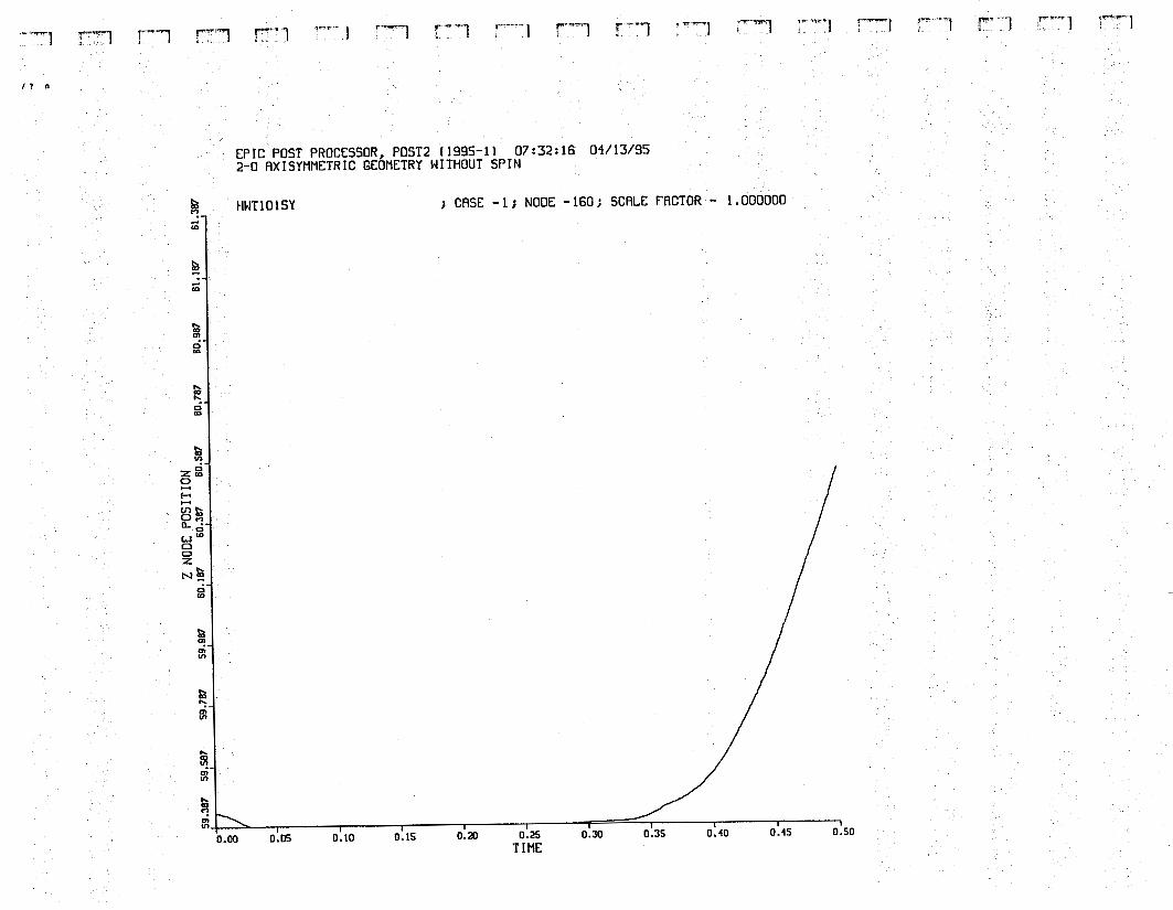
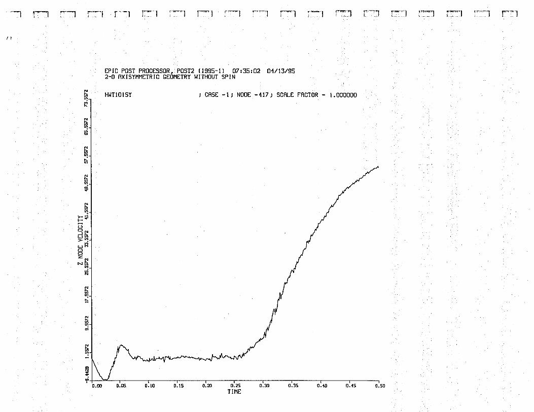
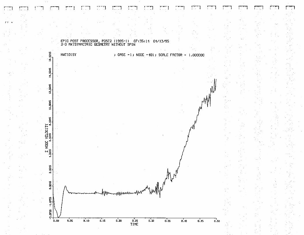
Figures 11 to 14 display the time history results of displacements and velocities at keylocations on the tank structure for both models.
The maximum hoop strain in the model with either code was calculated to be ~2%,which corresponds to a radial deformation of ~9 in. The annulus radial gap is 30 in.,which corresponds to a total strain of ~6.7%. Therefore, the primary liner does notcontact the secondary liner during the burn transient. The much higher primary linertransition region strain in the EPIC model is caused by an artificially imposed
thickness change that intentionally forces the strain location. However, is unclear whythis strain difference is such a large magnitude.
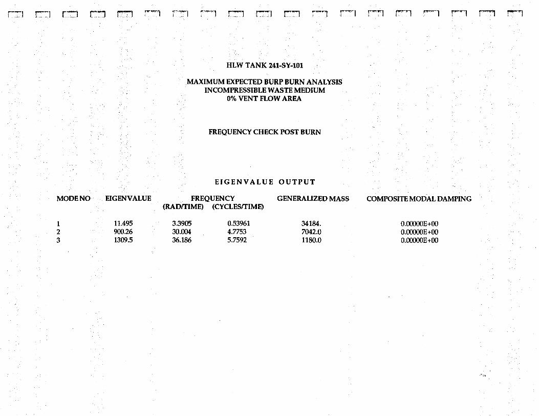
6.2. Reinforced Concrete Dome Fundamental Frequency ComparisonLANL performed an eigenvalue analysis of Tank 101-SY's dome structure9 using theABAQUS FEA tank model, which showed good correlation with theoretical solutions ofshallow spherical shells. The dome’s fundamental frequency was calculated to be ~7.5Hz, both with the FEA model and theoretical results. An eigenvalue extraction step wasappended to the present burn analysis to determine the dome’s fundamental frequencyafter material degradation has occurred from metal plasticity and concrete cracking.The ABAQUS results show that the dome’s fundamental frequency dropped to 0.54 Hz.
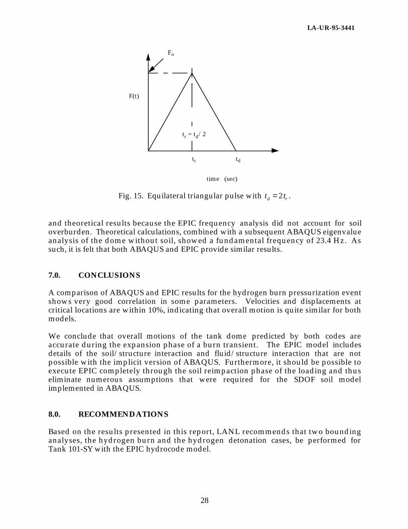
The EPIC frequency analysis consisted of applying a pressure pulse similar to thatshown in Fig. 15. A triangular pulse started at zero pressure, maximized at 5 psi in5 ms, and returned to zero pressure at 10 ms. This pulse caused dome apex motionsthat indicated a frequency of 23 Hz. This result differs from the ABAQUS analysis
LA-UR-95-3441
26
0
2
4
6
8
0.2 0.25 0.3 0.35 0.4 0.45
Displacement-Time HistoryEPIC Hydrocode Results
HaunchDome ApexDome 20 ft. radiusDome TransitionTank Base
Dis
pla
cem
ents
(in
.)
Time (sec)
Fig. 11. EPIC displacement-time history results.
- 1
0
1
2
3
4
5
6
7
0 0.05 0.1 0.15 0.2 0.25
Diplacement-Time HistoryABAQUS Finite Element Model
HaunchDome Apex20 ft RadiusTransitionTank Base
Dis
pla
cem
ent
(in
)
Time (sec)
Fig. 12. ABAQUS displacement-time history results.
LA-UR-95-3441
27
-20
0
20
40
60
80
0.2 0.25 0.3 0.35 0.4 0.45
Velocities-Time HistoryEPIC Hydrocode Results
HaunchDome ApexDome 20 ft. radiusDome transitionTank Base
Vel
oci
ties
(in
./se
c)
Time (sec)
Fig. 13. EPIC velocity-time history results.
-10
0
10
20
30
40
50
60
70
0 0.05 0.1 0.15 0.2 0.25
Velocity-Time HistoryABAQUS Finite Element Model
HaunchDome Apex20 ft RadiusTransitionTank Base
Vel
oci
ty (
in/
sec)
Time (sec)
Fig. 14. ABAQUS velocity-time history results.
LA-UR-95-3441
28
F(t)
time (sec)
Fo
tr td
tr = td/2
Fig. 15. Equilateral triangular pulse with td = 2tr .
and theoretical results because the EPIC frequency analysis did not account for soiloverburden. Theoretical calculations, combined with a subsequent ABAQUS eigenvalueanalysis of the dome without soil, showed a fundamental frequency of 23.4 Hz. Assuch, it is felt that both ABAQUS and EPIC provide similar results.
7.0. CONCLUSIONS
A comparison of ABAQUS and EPIC results for the hydrogen burn pressurization eventshows very good correlation in some parameters. Velocities and displacements atcritical locations are within 10%, indicating that overall motion is quite similar for bothmodels.
We conclude that overall motions of the tank dome predicted by both codes areaccurate during the expansion phase of a burn transient. The EPIC model includesdetails of the soil/structure interaction and fluid/structure interaction that are notpossible with the implicit version of ABAQUS. Furthermore, it should be possible toexecute EPIC completely through the soil reimpaction phase of the loading and thuseliminate numerous assumptions that were required for the SDOF soil modelimplemented in ABAQUS.
8.0. RECOMMENDATIONS
Based on the results presented in this report, LANL recommends that two boundinganalyses, the hydrogen burn and the hydrogen detonation cases, be performed forTank 101-SY with the EPIC hydrocode model.
LA-UR-95-3441
29
The analysis of the hydrogen burn case would be carried through past the instant whensoil overburden reimpacts on the dome. This analysis would provide a definitiveconclusion to questions regarding the consequences of soil (and pump pit) reimpactionand potential dome collapse and also would influence current SA conclusions for HLWTank 101-SY directly.
The hydrogen detonation case would provide a bounding quantitative estimate of tankfailure mechanisms and potential source terms for radiological and toxicologicalconsequences based on the dome collapse area.
ACKNOWLEDGMENT
This work was performed under funding from Westinghouse Hanford Company(WHC) in Richland, Washington, through the offices of Dr. J. Lentsch, HydrogenMitigation Operation, and Mr. G. D. Johnson, Flammable Gas Program. Thecooperation and assistance of the following individuals is greatly appreciated: Dr.Gordon Johnson and Ms C. R. Burns of ATI for the development of the initial EPICmodel; Dr. William Kubic, Mr. Robert Fujita, Dr. Steven Eisenhawer, and Dr. Jack Travisof LANL, who provided information on the burn and detonation gas dynamics andchemical kinetics; Dr. Kemal Pasamehmetoglu of LANL and Mr. Robert Marusich ofWHC, who provided the technical support and an impetus for performance of thiswork; Mr. Thomas Butler and Dr. Wilbur Birchler of LANL, who modified the ABAQUSmodel for the initial stages of the SA work; and Mr. L. J. Julyk of WHC, who providedthe original work of the structural analysis for HLW Tank 101-SY and detailed most ofthe groundwork.
REFERENCES
1. L. H. Sullivan et al., “A Safety Assessment for Proposed Pump Mixing Operations toMitigate Episodic Gas Releases in Tank 241-SY-101: Hanford Site, Richland,Washington,” Los Alamos National Laboratory report LA-UR-92-3196, Rev. 14 (May1995).
2. D. Hibbitt, B. Karlsson, and P. Sorensen, ABAQUS User’s Manual (HKS, Inc.,Providence, Rhode Island, 1992).
3. G. R. Johnson et al., User Instructions for the 1995 Version of the EPIC Code (AlliantTechsystems, Inc., Hopkins, Minnesota, November 1994).
4. J. A. Zukas et al., Impact Dynamics (Krieger Publishing Co., Malabar, Florida, 1992).
5. E. A. Rodriguez, T. A. Butler, and W. D. Birchler, “Structural Response of anUnderground Double-Shell Tank to a Hydrogen Burn Event,” Los Alamos NationalLaboratory report LA-UR-95-941 (March 1995).
LA-UR-95-3441
30
6. L. J. Julyk et al., “Structural Integrity Evaluation of Double-Shell-Waste Tank 241-SY-101 under a Postulated Hydrogen Burn,” Westinghouse Hanford Company reportWHC-SD-WM-TI-465 (April 1990).
7. P. M. Ferguson, Reinforced Concrete Fundamentals, 3rd ed. (Wiley & Sons, New York,New York, 1973).
8. R. E. Bolz and G. L. Tuve, CRC Handbook of Applied Engineering Science, 2nd Edition(CRC Press, Boca Raton, Florida, 1976).
9. E. A. Rodriguez and R. F. Davidson, “A Simple Model to Predict the FundamentalFrequency of the Reinforced Concrete Dome Structure of HLW Tank 101-SY,” LosAlamos National Laboratory report LA-UR-95-(TBD).
LA-UR-95-3441
31
APPENDIX A
TANK DETAILS
I-
-.-.-- &
I-
-7 \
I
n
c
n
F- i.: t f
i- F c-
y-’
LA-UR-95-3441
32
APPENDIX B
EPIC TIME-HISTORY AND MESH PLOTS
................
I-
i I r
i L-
\
.................
l- rn
................
.................
..................
\
.................. ....
.... -
..._.
t- .....
i
.... - I
.... ..................
..................
..................
.................. 1
u
i
............... ]z
............... 12
f h
8 E i= rn
v
0)
............... le I
...............
ll 2 0
1 2 3 4 5 6 7
-8
10 L 9
r
I- < 16
11 12 13 14 15
E. ..
- 17 18 19 20
I- L.,
24 4 25
k-. 26 27 28 29 30
c
r I
31 32 33 34 - 35
f: c,
r i
I- 1
Time-History PLOTS
Total Energy Kinetic Energy Internal Energy
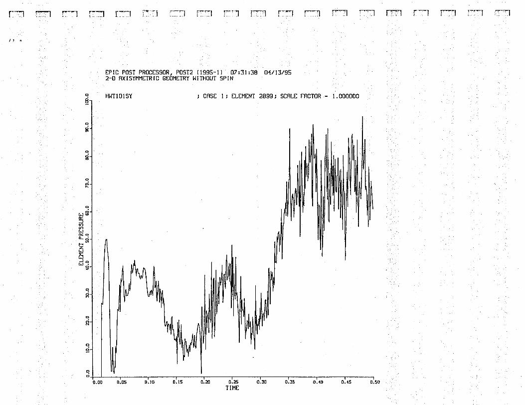
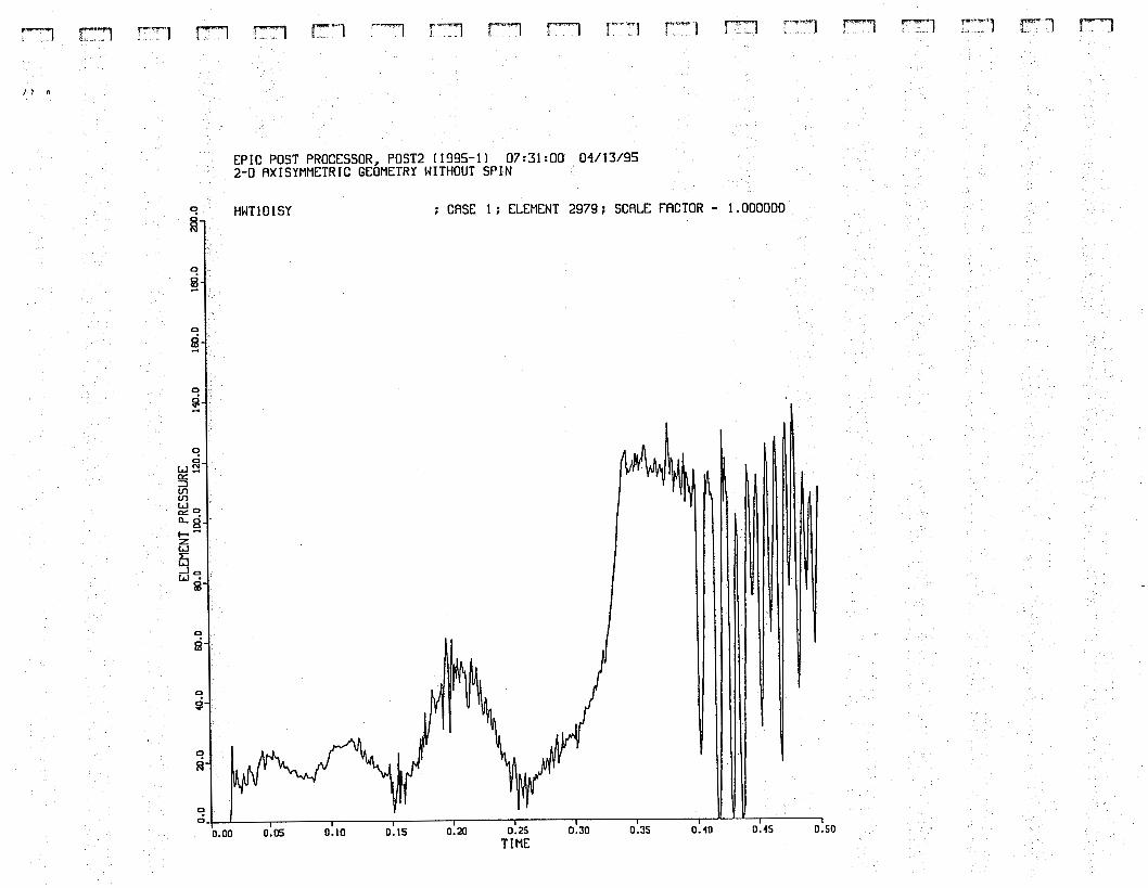
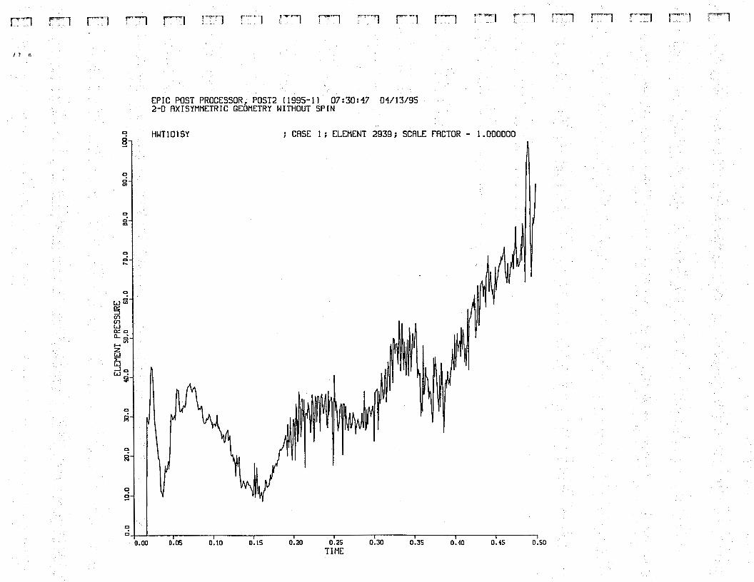
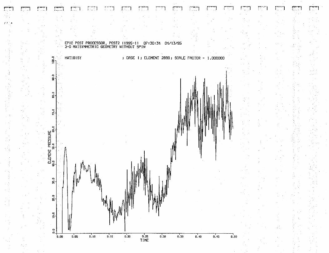
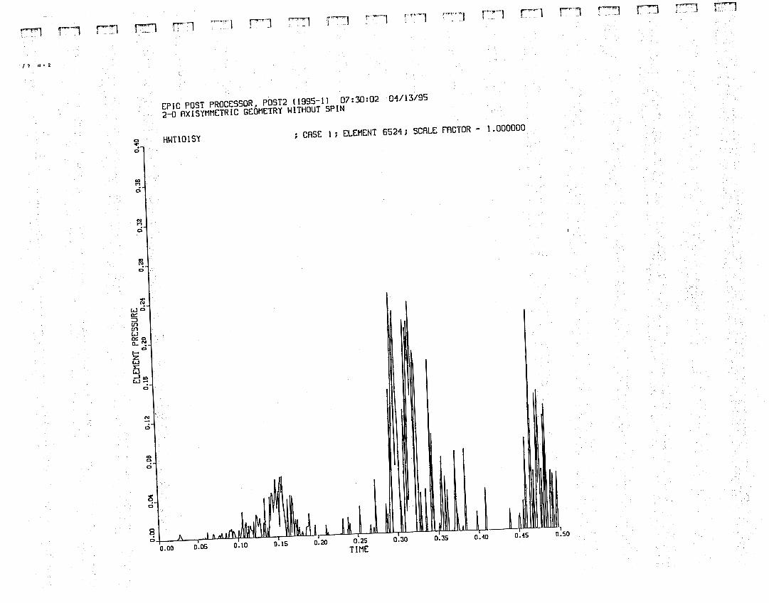
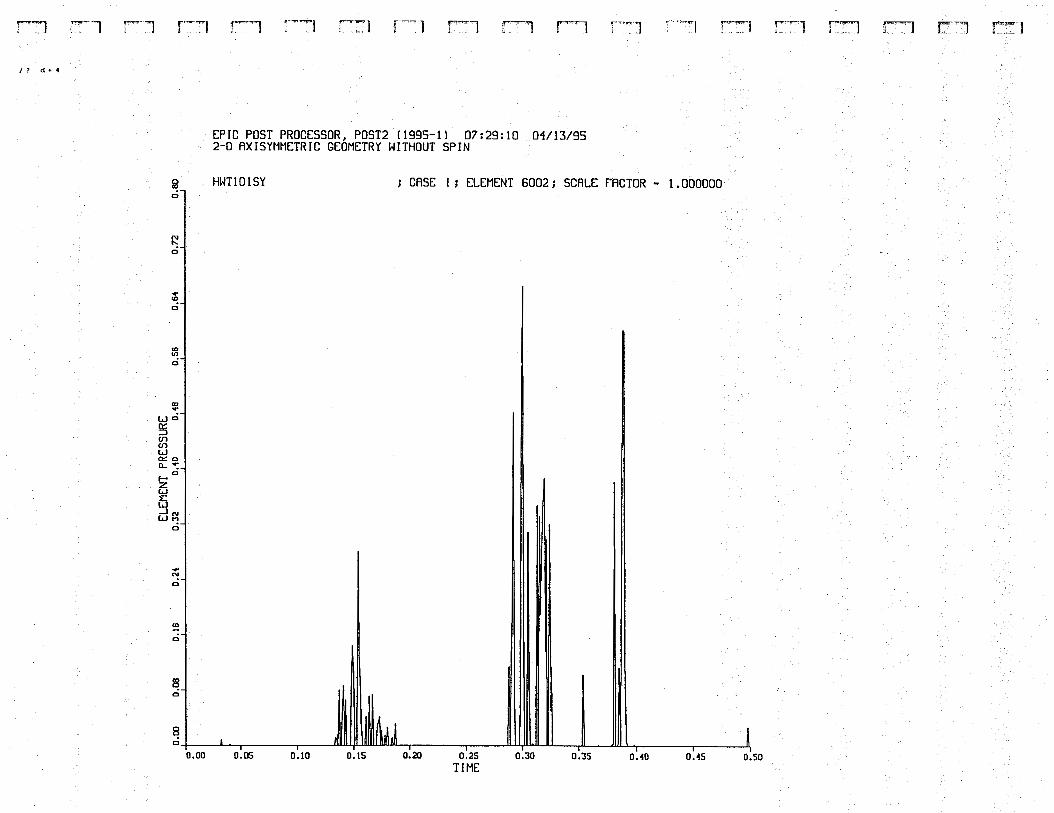
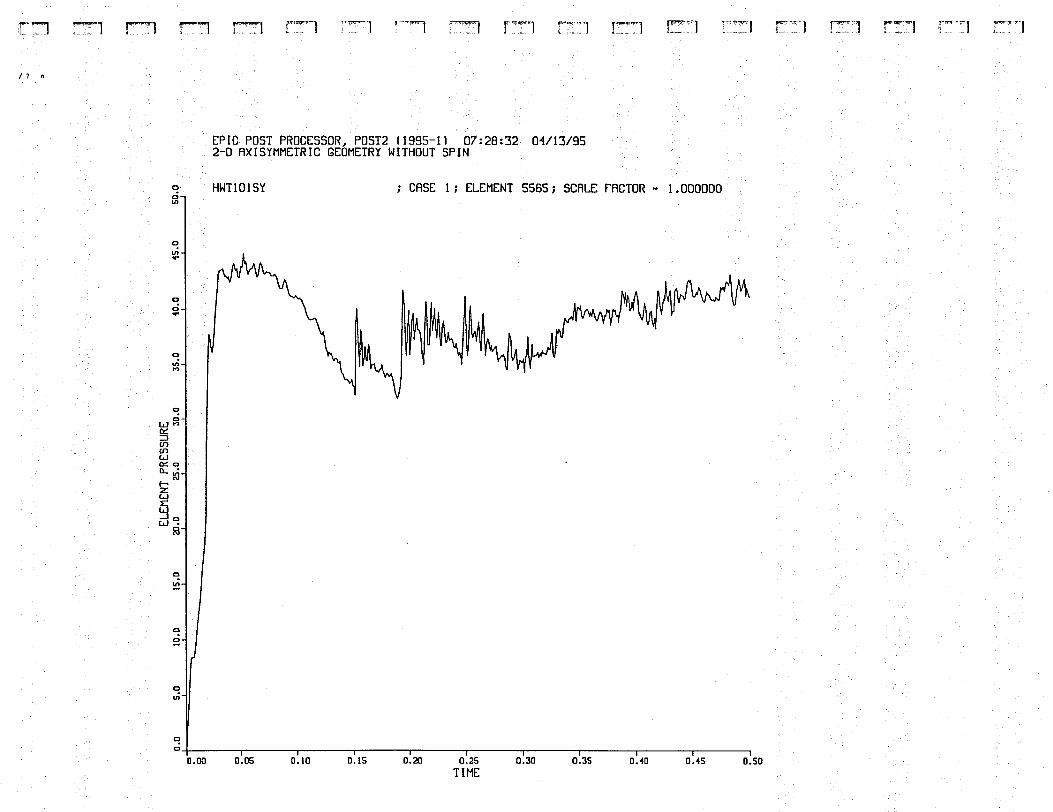
5489 - Soil. near CL Pressure Pressure Pressure Pressure Pressure Pressure Pressure Pressure Pressure Pressure Pressure Pressure Pressure Pressure 2 Position Z Position 2 Position 2 Position Z Position 2 Position 2 Position 2 Position Z Position Z Velocity 2 Velocity Z Velocity 2 Velocity 2 Velocity 2 Velocity 2 Velocity Pressure R Position
5541 - Soil; mid-tank 5565 - Soil, end-tank 5593 - Soil, near side 5637 - Soil, far side 6002 - H top near CL 6042 - H top middle 6670 - H top near side 6484- H bot near CL 6524 - H bot middle 6689 - H bot near side 2899 - Sludge near CL 2939 - Sludge near mid 2979 - Sludge near side
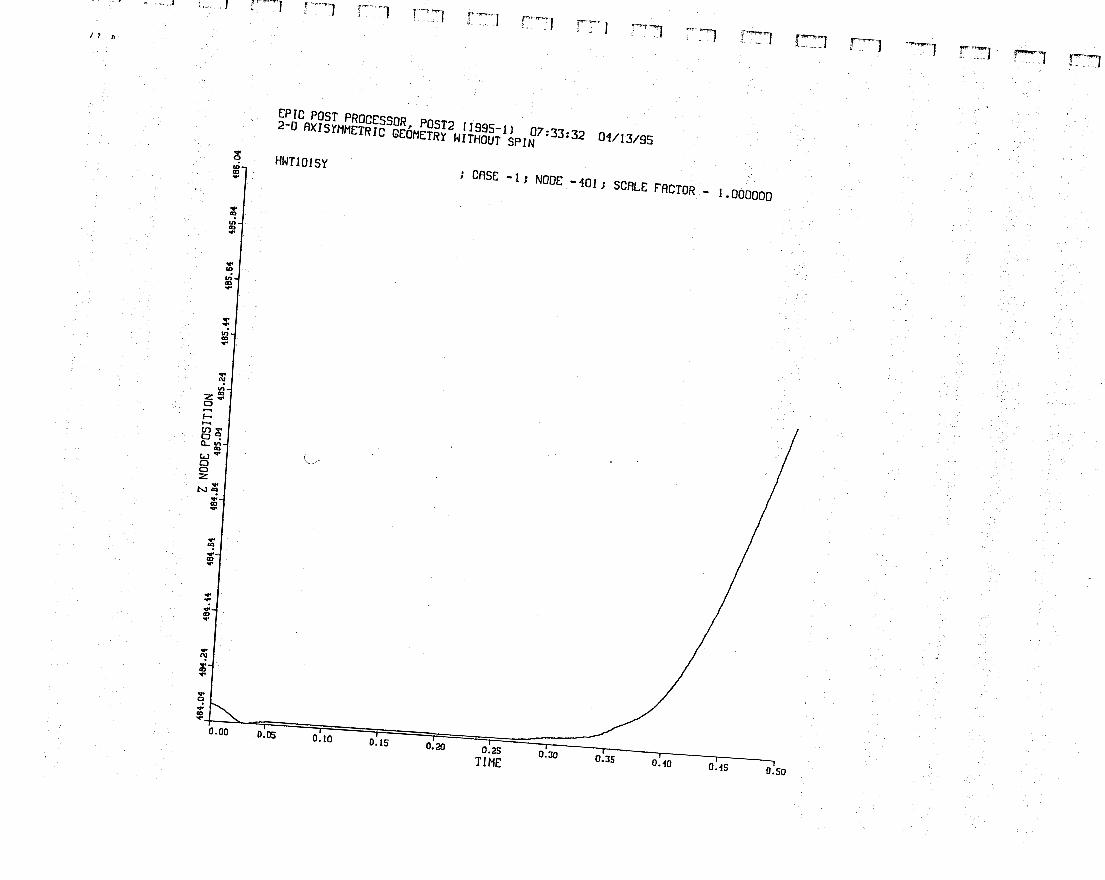
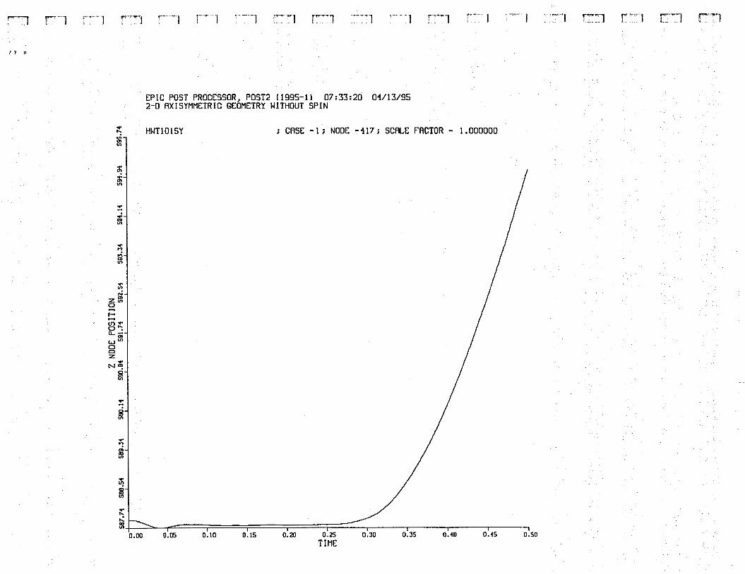
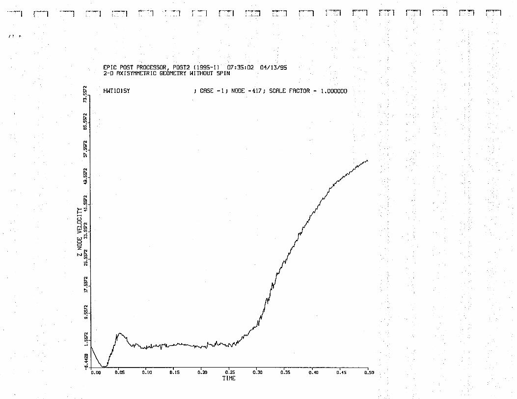
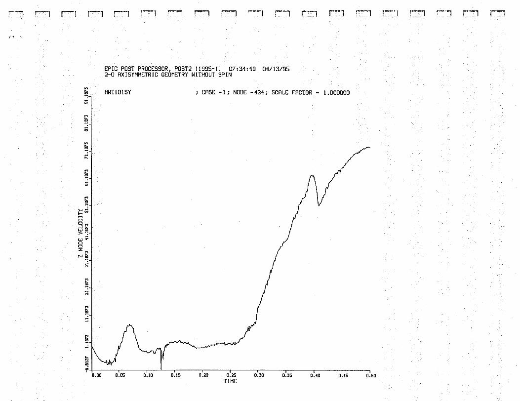
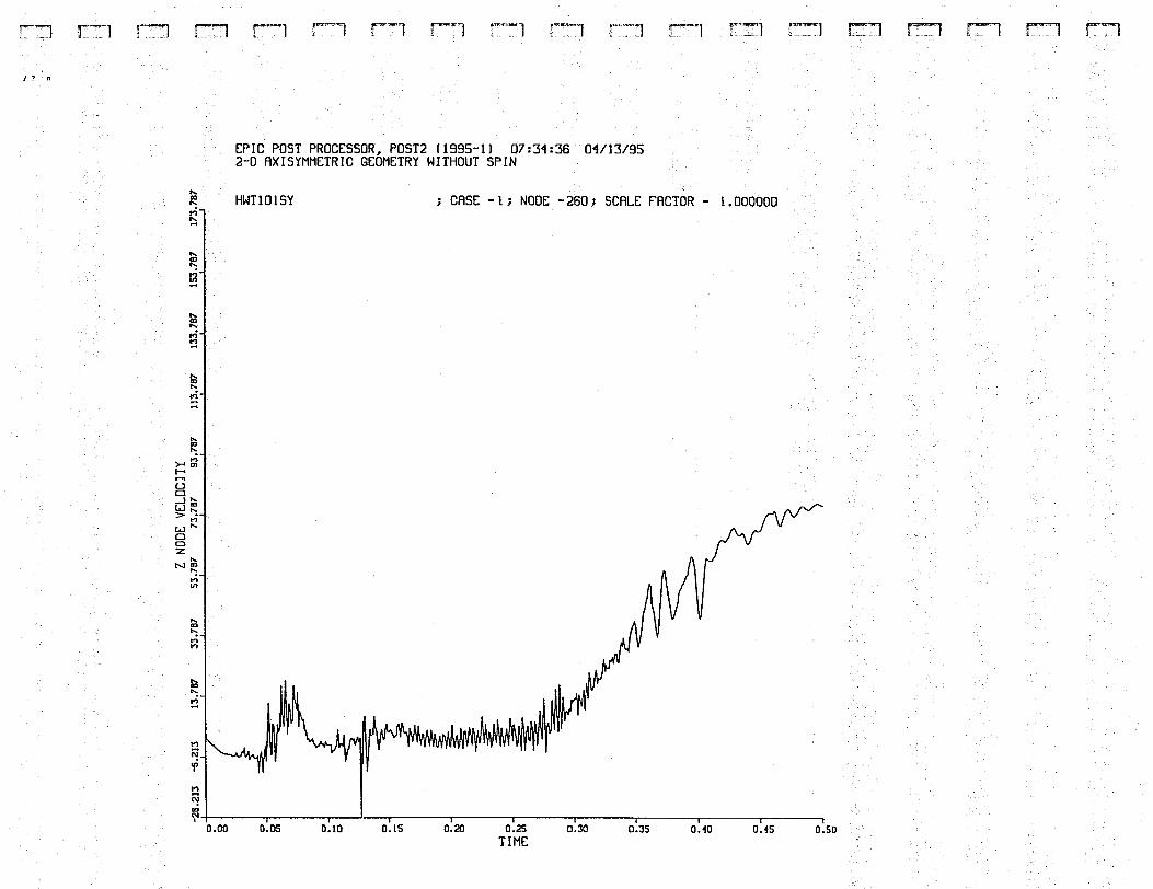
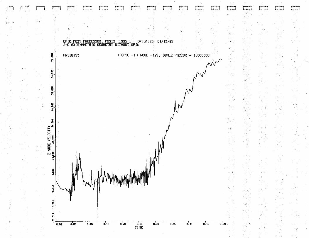
160 - Concrete side near bottom 3 14 - Concrete side (inside) at bottom 429 - Concrete Dome top CL 260 - Concrete Dome bot CL 424 - Concrete Dome Transition 417 - Concrete Dome 20 ' radius 401 - Concrete Dome Haunch
160 - Concrete side near bottom 314 - Concrete side (inside) at bottom 429 - Concrete Dome top CL 260 - Concrete Dome bot CL 424 - Concrete Dome transition 417 - Concrete Dome 20 ' radius 401 - Concrete Dome Haunch
739 - Crust middle
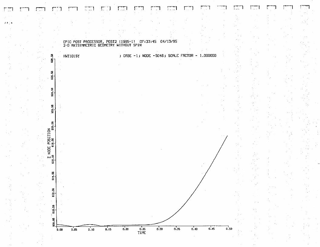
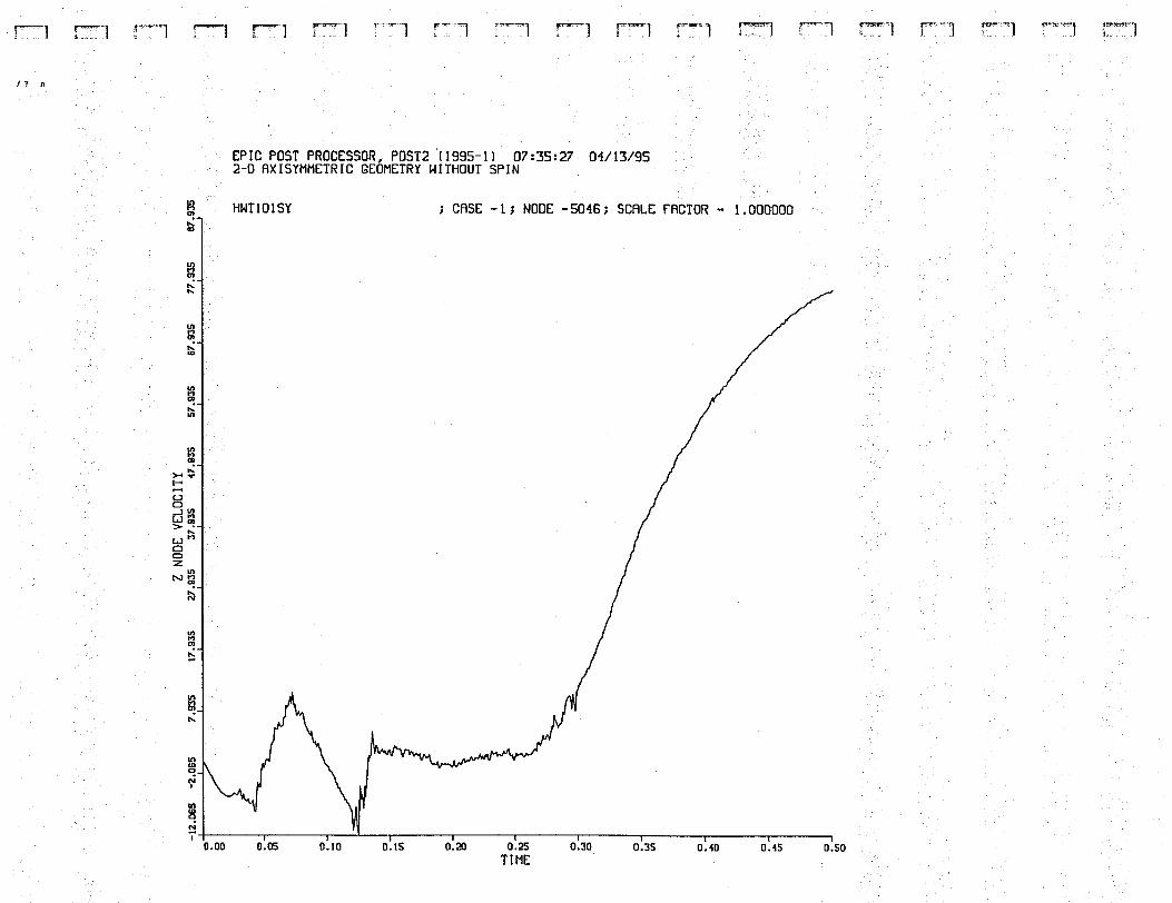
5046 - Pump Pit, bot near CL
5046 - Pump Pit, bot near CL
2016 - Primary liner mid-side
i- t... r i..
c
p: e i: h
*-
P t"
0
0
y1
E 0
In
0
?
w d 2
d
!
0
0
0
?
1.: , 1
r
i..
I. .,
m cn
\
$1
6
t ...
In
0
P
0
w
0
K? 0
0
0
9
z Bi
) t
.
P
i r. .
c
I i r- I
c.-
r- t - b; L,
t
3MS
S3tid lN3W313
Ls
I- ..,
i ..: !- .. h O
Z
-cn e
I 1
I I
I I
I I
I I
0'0s 0
'5t
O'O
t O'SE
0'0s O'SZ
0'02 O
'SI 0'01
0'5 0'
3MSS311d 1N3W
313
0
0
?
In
0
P
0
P
0
YI
0
T 0
0
".
mw
0-
t- ?E
Fa d 2 0
P
D
is 0
0
0 9
P
.-.
k..,
F-
r_
P-
I i.
-c(
x
N
f c. '
.
- 0
0
0 0
0 9
4
..
.y! 0
0
P ,. 0
0
0
P
..
m
0
?
0
0
?
mw
0- t.
?E
Fa d K? 0
s 0
e 0 0 9
0
F E...
Y 0
0
z 0
0
r 0
VI
0
?
0
2 mw
0
- e
NZ
R d !? n
0, 0
0
0
0 9
0
0
0 0
0
9 ..
i,
..,
r I
I I
I I
I I
I I
0'001 0'06
0-oe O'OL
om
0'0s
0.0) O'OE.
0'02 0'01
0' 3M
SS
3Ud LN3W313
\
w 0
0
e
I- i. .
.. 4
.. W
m
0
a ..
I I
I ,
I I
I
I I
I 0'002
0'081 0.091
O'abI
0'07.1 0'001
0'08 0'09
O'O
t O'UZ
0' 3M
SS3Lid 1N3LJ313
0
0
v!
Y)
P 0 0
P
0
In 0
?
0
0
'?
mw
0
-
f- N
r
a d i!? n
s 0 ? 0 0
0
?
0
0
vi
k2 0
0
w
0
In
0
?
0
0
c!
Inw
0
- *
cur
a d I? 0
s 0
4 0 9
0
0
0
0 0
0 0
9
4
I
fx 0
P L-
C
.. -
9; 0
r
t c.
h
OZ
-m
e 4
F
L L-
i
\
F
r In
Q) \
i.
r!
N
0
vf a
0 0 0 0
Y B
a
0
4
r
c .<
2
(2 w
.. z
x
01 W
h
d a:
.. -%
-
e c .I
0
P
0
r 0
0
i L
r I
I I
9 I
I I
I
I
I
08'0 ZL'O
C9'0
9s-0 8f.O
OC'O
ZE'O CZ'O
91'0
80'0 00'0
i 3M
SS
3tld 1N3W313
0
0
v!
z 0
0
P
0
tn
0 1
0
0 1
tnw
0
-
l- ?
X
w d 2
0
2
0
? 0
0
0
9
\
v 0
i.
co a
r --
&
r
t tl
Ln m
\
M
\
v 0
Ln Y. M c
t ." .
W 0 0
z
d
.. I
W
v)
CT 0
..
1
a a 3 1
? ¶ ? YW
1- i- ?E
J ?
F
i- t..
LL
W
d 0 v) .. 4 I
W 0
0
z
.. 4
I
W
u)
(Is
0
-.
i k’
t
:
i i. .
d
.. In3
It
-
UIO
!- i i
M
M
-cI 3
N
NOflfSOd 300N Z
P
\
r
\
v 0
W 0
0
z
.-I
.. I
w
cn U
0 -.
cu M
I
h .. az e -cn d
c
t k..
F- r L :z
F
L...
13 f: r -.
P
1. 7
i I,
t b,
0 .. 2 I
W 0 0
z 4
.. I
-4
0
v)
0
m 0
P
0
P
0
v1
2 0
0
'?
mu
0
-
c- N
r=
$3 d 2
0
P
0
ls 0 8 0
F
b
F
\
..
c
i /i
/
P; 0
+
.4
I -. c-
b t.
c
t.-.
r^
t- i
.v! 0
0
In - 0 .. 0
P
0
..
In
0
.T!
0
x lnw
0-
c- ?X
R d
.. 2
0
5
0
II! 0 0
0
9
3013 3OON 2
r
i; t c
Y 0 0
z 0 0
.p
0
VI
0
T
0
0
1
vlw
0
- e
?X
R d 2
0
s! 0
rs 0
0
9
0
k- t... 6
0
cu
r i, b
c * i
.
0
0
yf
ln
f
0
0
P
0
Ln
0
T? 0
0
T?
tnw
?E
0-
t-
a d 2
0
P
0
4 0 0
9 0
v
!? az h
-m e
r
&:
s-^ .
LY 0
r
W
a 0
Lo
.. \
W 0
0
z
w 0
ul P
0
0
P
0
v)
0
'?
0
2 tnw
0
-
c-
R d 5 0
0
is 0
!
0
.y! 0
0
in
0
.?
.P 0
0
in
0
.?
.'? 0
0
inw
0-
f- .?
a 'd
.. 2
0
P
.. 0
23 ,. 0
0
.o
9
i I
.v! 0
0
In
- 0 .. 0
0
.x
.T? In
0
0
0
T? ww
0
-
t- ?E
R d
.. !!? 0
0
0
.. d
8 .. a
0
.o
9
R. :1
4
I
tY 0
w
0
Q
LL W
-1
Q
0
cn
0
.. 2 I
w 0
0 2
4
.. I
W
cn c
0
.. r x L I
I
I
I
I I
I
I
1 I
989S*fi 989S'TI:
989S'RZ
989S'SZ
9WS'IZ
9WS'A 989S'lt
9895.6
989S'S
9895'1 G
IB'
JL13013h 300N 2
In
cn \
\
1p 0
r!
M 0
.. M Lf! h
OZ
-m a
d
0
I
W 0
-1
0
* .. 0 0 0
0 0
0 0
0
I
W
+
9
E# .. - I
# c 0 .. I
W
tn ZI
W
cn @
= c 0
0 0'0001 r
- I
0'006 - a
c
.

R
r- i.
F
0
..
r- W
z
.. c-.
5-
i c
M
.. !?
-
P-
0' '0001 I
0.00s 0.OOZ
O*OOI 0' 0
SIXU z

i
c P L.
-u
3
0 '000 1 I
0
N
0
5 0
n,
--.
8 0 i
VI
01 \
s?
c-
r
c.
0'
N
U
.
0
..
3 .E! 9
W
x 9 z 0

I
w
J
0
G ..
GI-
..
I IIR
II L
0
I
W
-1
0
r u .. 0
co LD
8 0 rl 0
c 0
I !-- L
h
t b W
V
I Q
: 0
..
L- .
I
cn W
S
i- t. 0
N

0' '000 1 I
0
N
I-
k'
t,,
W
-1
u
* 0
!?
-
q-
.. r t,
I
..
6 0' '000 I r
N

w.
$
h e
--v,
.4 I
C.
P i
E- li
d In
0
0'0001 O
"6
0'008
0'009 0'005
O'OOC o*m
t 0'002
0'001 0'0
N

r
I
w
9
s O
8 0 7
0'0
SIXH
2
I
W
Ln a 0
..
F- a,
L
LA-UR-95-3441
33
APPENDIX C
ABAQUS TIME-HISTORY PLOTS AND RESULTS
FOR ZERO WASTE FLUID RADIAL MASS
LA-UR-95-3441
34
APPENDIX C
The results contained in this appendix pertain to the modeling assumption using 0% ofthe radial waste fluid mass as participating actively in a dynamic environment. Theoriginal ABAQUS analyses contained in the SA provide results based on the assumptionthat 50% of the radial waste fluid mass is participating actively in a dynamic transient.
These results are reported herein as part of the comparison between ABAQUS andEPIC and are consistent with the fluid/structure interaction results of EPIC.
For information only, the 50% radial waste fluid mass results are presented in App. F.
09 0
Y
0
0
L cu 0
v)
Y
0
* 0 v)
0
9
0
..__ .....................
;_. .....
......
......
..... i
.....................
.....................
.....................
.....................
.....................
.....................
.....................
F
L..:
....
L
f
9
9
f
9
-r d
F
4
4
4
4
s 4
4
......................... \
................................
............... ' ................
m T! 0
T! 0
In
8 0
r L
.a
E[ rn 3: ................. .... .....
L
s
....
....
.... .,..
i
.................
u
.....
x .....
.....
.,...
L \ ................. I
............... & ............... 4
0
v)
Y
0
\
.....
.....
......
.,...
i
Y
0
Y
.............
II 8
3 2 .............
X 0
)
............
T! 0
t L
............. ) ...........
) u
I; c --a
0
...................................
\
............... < ................
..
........ ...........................
m
0
cu 2 m
* 0 T! 0
m 2 0
m
0
h!
r\l 0
m
T! 0
m
8 0
+ ............... \
I,
,
/I
,
I,
,
................. < .................... ; ...............
.........................................................
...... ~
......................................
.................
\ ............... .................
.................
1 I
.............. {a
1.
t
c
i .: ...........
t
2' j 1;
L;
\ 'i
.............. +....... . -
.................................
1 I \
...............
'\
................
- -r :- .!..
y A ....
i
P .- ....
.p. ..
i
m
iJ
j
cu 0 m
T? 0
T? 0
m
8 0
F
F! 0
m
0
T!
T! 0
m
8 0
In
0
n! T
Y
0
r
e .. ...............
1 __._.
.....
r
I t In
T! 0
.e.. ................
................
................
i- t L
................
jl 2
E: 2 a”
I- i 0
.... ....
....
In
8 ....
i L.
d
r 0
In
N
0
Y
E tn
i-
t. " t
\ ................ - .... .....
.....
J- lj
x
t
r L,
...................... ....
g :I
.,.. .... ....
i ...................
\ d ....
.,..
Y
0
In T! 0
T! 0
In
8 0
R In
0
LA-UR-95-3441
35
APPENDIX D
FREQUENCY ANALYSIS DETAILS
5 W
E
e t,
..
88
8
++
+
LA-UR-95-3441
36
APPENDIX E
EPIC MATERIAL MODELS
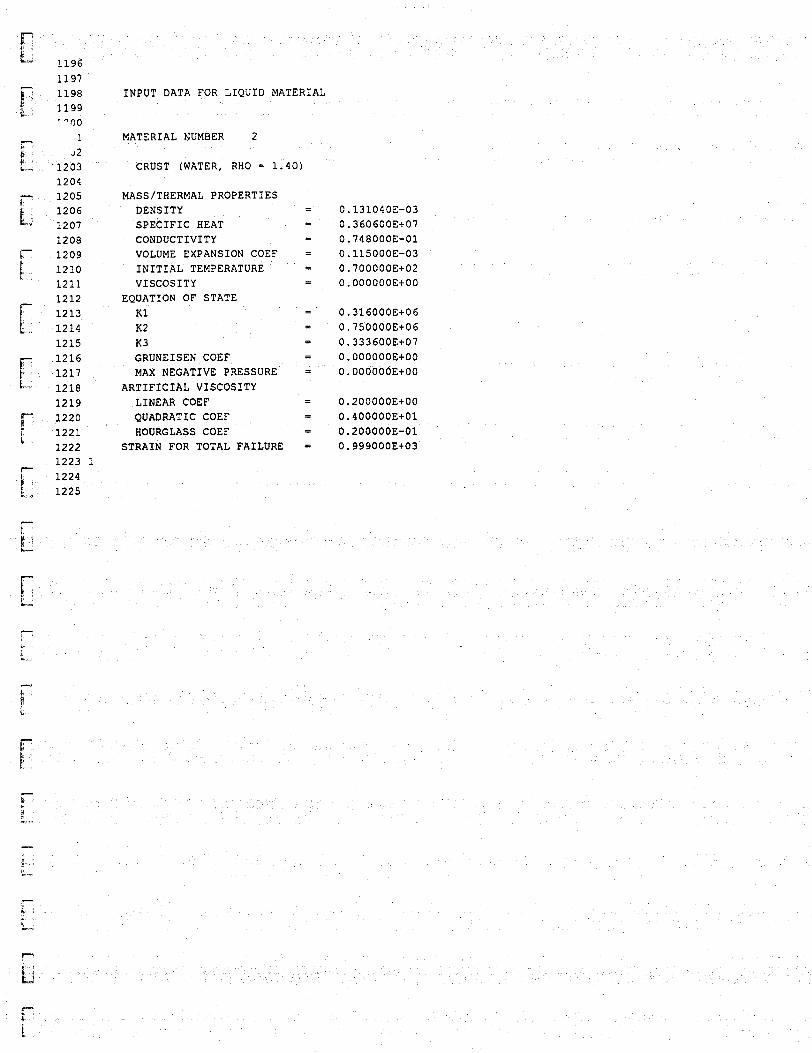
1197
::;; INPUT DATA FOR LIQUID MATERIAL
- '00 r !.I 1203 CRUST (WATER, RHO = 1.40)
1 MATERIAL NUMBER 2 J2
1204 - 1205 1206 iL 1207
1208 r 1209 1 , 1210
1211 1212 r 1213
t_, 1214 1215
r 1216 ' 1217
6- - 1218 12 19
r- 1220 E ' 1221
i. 1222 1223 1 -
MASS/THERMAL PROPERTIES DENSITY SPECIFIC HEAT CONDUCTIVITY VOLUME EXPANSION COEF INITIAL TEMPERATURE VISCOSITY
EQUATION OF STATE K1 K2 K3 GRUNEISEN COEF MAX NEGATIVE PRESSURE
ARTIFICIAL VISCOSITY LINEAR COEF QUADRATIC COEF HOURGLASS COEF
STRAIN FOR TOTAL FAILURE
= 0.131040E-03 = 0.360600E+07 = 0.748000E-01 = 0.115000E-03 = 0.700000E+02 = 0.000000E+00
= 0.316000E+06 = 0.750000E+06 = 0.333600E+07 = 0.000000E+00 = 0.000000E+00
= 0.200000E+00 = 0.400000E+01 = 0.200000E-01 = 0.999000E+03
1224 1.: 1225
1227
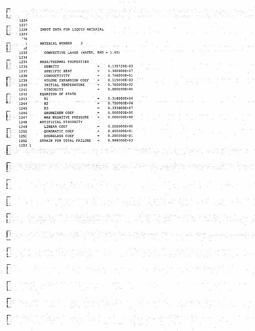
&A 1229 Ep: 1228 INPUT DATA FOR LIQUID MATERIAL
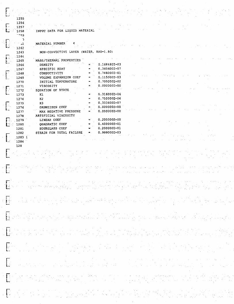
1256 1257 1258 INPUT DATA FOR LIQUID MATERIAL
1286 1287
b, 1288 INPUT DATA FOR LIQUID MATERIAL '99
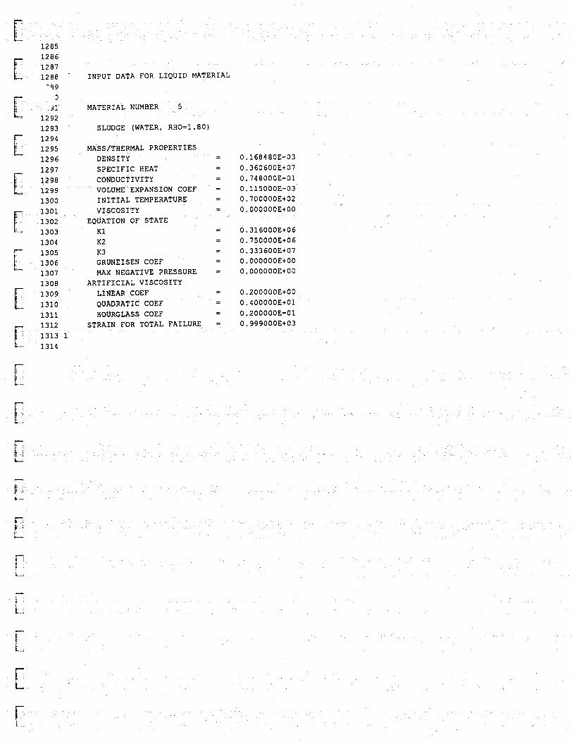
MATERIAL NUMBER 5
12 93 SLUDGE (WATER, RHO=1.80) F 1294
LJ lzg5 MASS/THERMAL PROPERTIES 1296 DENSITY = 0.168480E-03 12 97 SPECIFIC HEAT = 0.360600E+07 12 98 CONDUCTIVITY = 0.748000E-01 1299 VOLUME EXPANSION COEF = 0.115000E-03 1300 INITIAL TEMPERATURE = 0.700000E+02
VISCOSITY = 0.000000E+00 EQUATION OF STATE
K1 = 0.316000E+06 1304 K2 = 0.750000E+06 1305 K3 = 0.333600E+07
GRUNEISEN COEF = 0.000000E+00 1307 MAX NEGATIVE PRESSURE = 0.000000E+00 1308 ARTIFICIAL VISCOSITY 1309 LINEAR COEF = 0.200000E+00 1310 QUADRATIC COEF = 0.400000E+01 1311 HOURGLASS COEF = 0.200000E-01
r 1306 c - *
1312 STRAIN FOR TOTAL FAILURE = 0.999000Et03 1313 1
k . 1314
'16 INPUT DATA FOR SOLID MATERIAL 7 r8
1419 MATERIAL NUMBER 8 1420
r 1421 LINER STEEL 1 1422 i( 1423
1424 1425
%; 1426 1427 1428 1429
.-' 1430 1431
!- 1432 ' 1433
1434 1435
r 1436 ' 1437
1438
1442 1443
'4 .5
1446
1449 1450 1451
t , 1 1452 1453 1454 1455 1456 1457 r 1458
b , 1459 14 60 1461 1462
L - * 1463 1 14 64
r 1465
MASS/THERMAL PROPERTIES DENSITY = 0.738000E-03 SPECIFIC HEAT = 0.389700E+06 CONDUCTIVITY = 0.908000E+01 VOLUME EXPANSION COEF = 0.180000E-04 INITIAL TEMPERATURE = 0.700000E+02 ROOM TEMPERATURE = 0.700000E+02 MELTING TEMPERATURE = 0.280000E+04 ABSOLUTE ZERO TEMP = -0.459670E+03
STRENGTH PROPERTIES FOR JOHNSON-COOK MODEL SHEAR MODULUS = 0.116280E+08 YIELD STRESS, C 1 = 0.330000Ei05 HARDENING COEF, C2 = 0.135000E+06 HARDENING EXPONENT, N = 0.600000E+00 STRAIN RATE COEF, C3 = 0.100000E-01 SOFTENING EXPONENT, M = 0.100000E+01 PRESSURE COEF, C4 = 0.000000E+00 MAX STRENGTH (OPTIONAL) = 0.900000E+05
EQUATION OF STATE FOR MIE-GRUNEISEN MODEL K1 = 0.230490E+08 K2 = 0.749600E+08 K3 = 0.750625E+09 GRUNEISEN COEF = 0.169COOEi01 MAX NEGATIVE PRESSURE = 0.100000Et08
ARTIFICIAL VISCOSITY LINEAR COEF = 0.200000E+00 QUADRATIC COEF = 0.400000E+01 HOURGLASS COEF = 0.200000E-01
FRACTURE PROPERTIES FOR JOHNSON-COOK MODEL DAMAGE COMPUTED E 0 FRACTURE ALLOWED - 0 Dl = 0.24000CE+00 D2 = 0.000000E+00 D3 = 0.10OOOOE+01 D4 = 0.000000E+00 D5 = 0.000000E+00 MINIMUM FRACTURE STRAIN = 0.240000E+00 SPALL STRENGTH = 0.680000E+06 DAMAGE SOFTENING FACTOR = 0.000000E+00
STRAIN FOR TOTAL FAILURE = 0.240000E+00
-
1317 1318 INPUT DATA FOR SOLID MATERIAL 1319 .I 20
6- 1 MATERIAL NUMBER 6 .LZ
1323 REBAR STEEL 1324 1325 1326
&- 1327 1328 1329 hi : ', 1331 1330
1332
1335 1336
E 1338 1337
1339 1340 1341 1342 1343 1344 1345 1346 1.347
'8 '9
1350
c
1354 1355
P f;; 1356
1357 1358 r 1359
ki 1360 1361
~ 1363 1364 1365 1
k :_(
1
MASS/THERMAL PROPERTIES DENSITY = 0.738000E-03 SPECIFIC HEAT = 0.389700E+06 CONDUCTIVITY = 0.908000E+01 VOLUME EXPANSION COEF = 0.180000E-04 INITIAL TEMPERATURE = 0.700000E+02 ROOM TEMPERATURE = 0.700000E+02 MELTING TEMPERATURE = 0.280000E+04 ABSOLUTE ZERO TEMP = -0.459670E+03
STRENGTH PROPERTIES FOR JOHNSON-COOK MODEL SHEAR MODULUS = 0.116280E+08 YIELD STRESS, C1 = 0.600000E+05 HARDENING COEF, C2 = 0.250000E+06 HARDENING EXPONENT, N - 0.600000E+00 STRAIN RATE COEF, C3 0.100000E-01 SOFTENING EXPONENT, M = 0.100000E+01 PRESSURE COEF, C4 = 0.000000E+00 MAX STRENGTH (OPTIONAL) = 0.120000E+06
EQUATION OF STATE FOR MIE-GRUNEISEN MODEL K1 - 0.230490E+08 K2 = 0.74 9600E+08 K3 = 0.750625E+09 GRUNEISEN COEF = 0.169000E+01 MAX NEGATIVE PRESSURE = 0.100000E+08
ARTIFICIAL VISCOSITY LINEAR COEF = 0.200000E+00 QUADRATIC COEF = 0.400000E+01 HOURGLASS COEF 0.200000E-01
FRACTURE PROPERTIES FOR JOHNSON-COOK MODEL DAMAGE COMPUTED 0 FRACTURE ALLOWED = 0 Dl = 0.800000E-01 D2 = 0.000000E+00 D3 = 0.100000E+01 D4 = O.OOOOOOE+OO D5 = 0.000000E+00 MINIMUM FRACTURE STRAIN 0.800000E-01 SPALL STRENGTH = 0.680000E+06 DAMAGE SOFTENING FACTOR = 0.000000E+00
STRAIN FOR TOTAL FAILURE 5 0.800000E-01
. .
5 ,4 6 MATERIAL NUMBER 14
1547 1548 STRUCTURAL CONCRETE 142 PCF 5900 PSI 1549 1550 MASS/THERMAL PROPERTIES 1551 DENSITY = 0.2130OOE-03 1552 SPECIFIC HEAT = 0.563000E+06 1553 CONDUCTIVITY = 0.220000E+00 1554 VOLUME EXPANSION COEF = 0.240000E-04 1555 INITIAL TEMPERATURE = 0.700000Zt02 1556 STRENGTH PROPERTIES
[ 1558 1557 SHEAR MODULUS = 0.237900Et07
COMPRESSIVE STRENGTH, F'C= 0.590000Et04
7 Ld
f - -
1 6 3 7
1 6 3 9 1 6 3 8 INPUT DATA FOR CRUSHABLE MATERIAL (MODIFIED HULL MODEL)
- C40 i - ,
i- 1
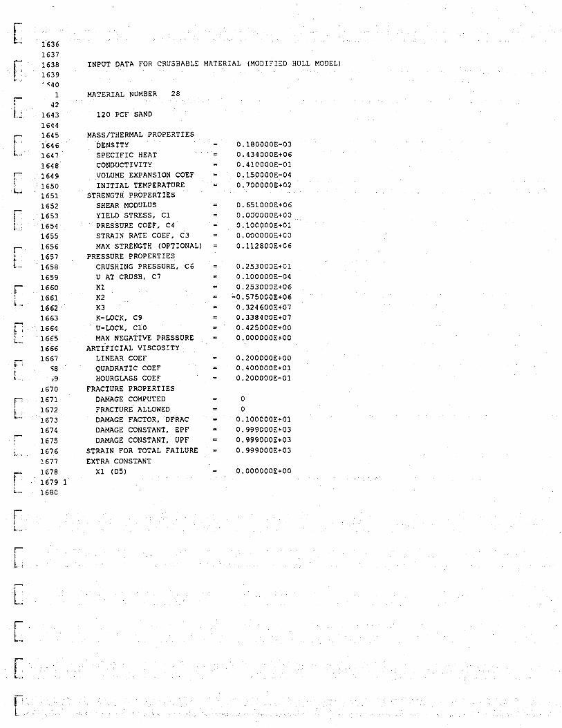
42 MATERIAL NUMBER 2 8
t i 1 6 4 3 1 2 0 PCF SAND 1 6 4 4 r 1 6 4 5 MASS/THERMAL PROPERTIES 1 6 4 6 DENSITY
e‘- 1647 SPECIFIC HEAT
= -
1 6 4 8 CONDUCTIVITY - - r 1 6 4 9 VOLUME EXPANSION COEF = r; 1 6 5 0 I N I T I A L TEMPERATURE
1 6 5 1 STRENGTH PROPERTIES 1 6 5 2 SHEAR MODULUS 1 6 5 3 YIELD STRESS, C1
=
- - r L,, 1 6 5 4 PRESSURE COEF, C4
- - - -
1 6 5 5 STRAIN RATE COEF, C 3 1 6 5 6 MAX STRENGTH (OPTIONAL) = 1 6 5 7 PRESSURE PROPERTIES
- -
r -1- 1 6 5 8 CRUSHING PRESSURE, C6 =
1 6 5 9 U AT CRUSH, C7 =
6 1 6 6 0 K 1 ! 1 6 6 1 K2 - b.” 1 6 6 2 K3
1 6 6 3 K-LOCK, C9 1 6 6 4 U-LOCK, C10
1
- - - - - -
i , 1 6 6 5 MAX NEGATIVE PRESSURE = 1666 ARTIFICIAL VISCOSITY 1 6 6 7 LINEAR COEF -
f 58 QUADRATIC COEF
[I 1 6 7 2
- j9 HOURGLASS COEF
I 670 FRACTURE PROPERTIES 1 6 7 1 DAMAGE COMPUTED
- -
=
FRACTURE ALLOWED - - 1 6 7 3 DAMAGE FACTOR, DFRAC 1 6 7 4 DAMAGE CONSTANT, EPF 1 6 7 5 DAMAGE CONSTANT, UPF
- - - - - -
1.. 1 6 7 6 STRAIN FOR TOTAL FAILURE = 1 6 7 7 EXTRA CONSTANT
0 . 1 8 0 0 0 0 E - 0 3 0 . 4 3 4 0 0 0 E + 0 6 0 .410000E-01 0 .150000E-04 0 . 7 0 0 0 0 0 E + 0 2
0 0
0.100000E+01 0 . 9 9 9 0 0 0 E + 0 3 0 . 9 9 9 0 0 0 E t 0 3 0 . 9 9 9 0 0 0 E + 0 3
1 6 7 8 X 1 (D5) f 1 6 7 9 1 = 0 . 0 0 0 0 0 0 E + 0 0
L 1 6 8 0
1683
[ 1685 . c(86
- ~ . ~
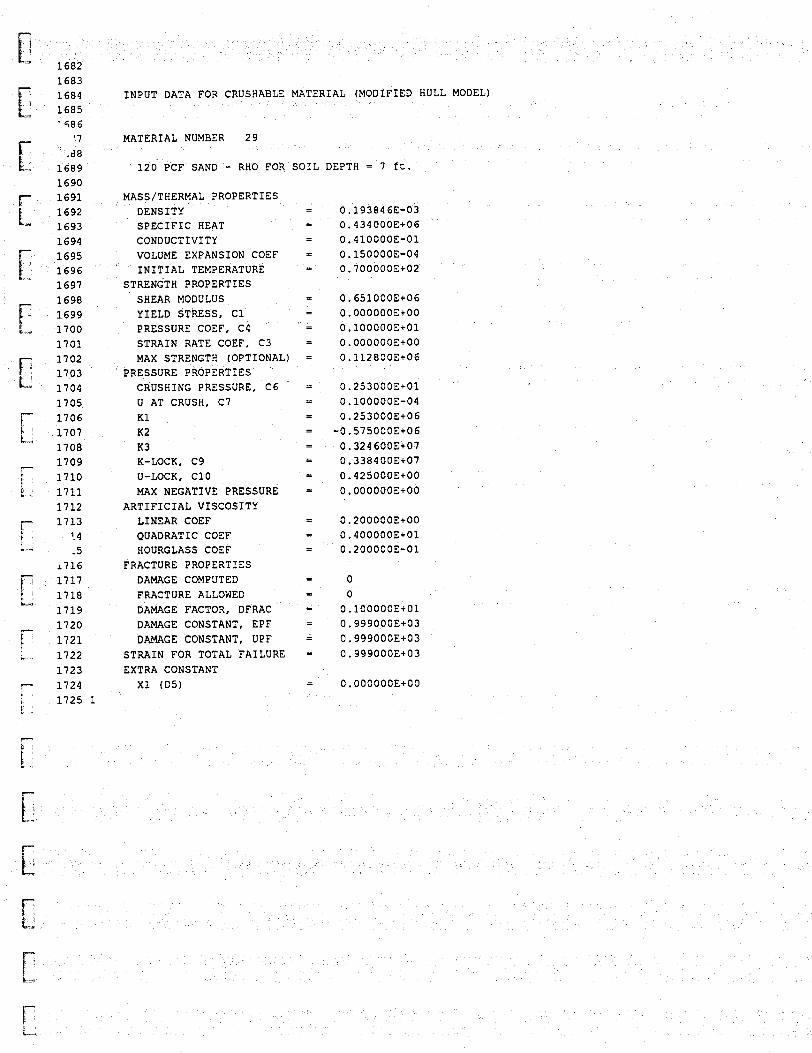
1684 INPUT DATA FOR CRUSHABLE MATERIAL (MODIFIED HULL MODEL)
MATERIAL NUMBER 29
120 PCF SAND - RHO FOR SOIL DEPTH 7 ft. 1690
6 1691 1692 1693 1694 1695 1696 1697 1698
f 1699 ba 1700
1701
1705 1706 r. 1708 1709 r 1710 1711 1712 1713 1.4 -5
1716 E- 1717
' 1718 L" 1719 1720
r I c. .,
1721 L . 1722
1723 7 1724
MASS/THERMAL PROPERTIES DENSITY SPECIFIC HEAT CONDUCTIVITY VOLUME EXPANSION COEF INITIAL TEMPERATURE
STRENGTH PROPERTIES SHEAR MODULUS YIELD STRESS, C1 PRESSURE COEF, C4 STRAIN RATE COEF, C3 MAX STRENGTH (OPTIONAL)
PRESSURE PROPERTIES CRUSHING PRESSURE, C6 U AT CRUSH, C7 K1 K2 K3 K-LOCK, C9 U-LOCK, ClO MAX NEGATIVE PRESSURE
ARTIFICIAL VISCOSITY LINEAR COEF QUADRATIC COEF HOURGLASS COEF
FRACTURE PROPERTIES DAMAGE COMPUTED FRACTURE ALLOWED DAMAGE FACTOR, DFRAC DAMAGE CONSTANT, EPF DAMAGE CONSTANT, UPF
STRAIN FOR TOTAL FAILURE EXTRA CONSTANT X1 (D5)
1 1725 1 i
0,193846E-03 0.434000E+06 0.410000E-01 0.150000E-04 0.700000Et02
0.651000Et06 0.000000E+00 0.100000E+01 0.000000E+00 0.112800E+06
0.253000Et01
0.253000Et06 0.100000E-04
-0.575000Et06 0.324600Et07 0.338400Et07 0.425000Et00 0.000000E+00
0.200000E+00 0.400000E+01 0.200000E-01
0 0 0.100000E+01 0.999000Et03 0.999000Et03 0.999000Et03
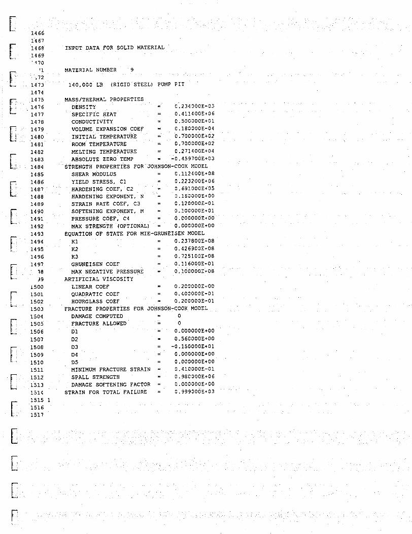
1467 14 68 I N P U T DATA FOR S O L I D M A T E R I A L 1469
1515 1 1516
k-.* 1517
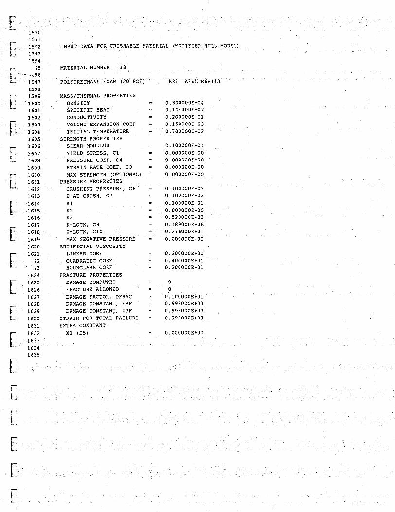
! 1591 1592 INPUT DATA FOR CRUSHABLE MATERIAL (MODIFIED HULL MODEL) 1593
35 MATERIAL NUMBER 18 --__ ' --,96
1597 POLYURETHANE FOAM (20 PCF) REF. AFWLTR68143
LA-UR-95-3441
37
APPENDIX F
ABAQUS TIME-HISTORY PLOTS AND RESULTS
FOR 50% RADIAL WASTE FLUID MASS

LA-UR-95-3441
38
APPENDIX F
The results contained in this appendix pertain to the modeling assumption using 50% ofthe radial waste fluid mass as participating actively in a dynamic environment. Theoriginal ABAQUS analyses contained in the SA provide results based on thisassumption.
These results are not reported as part of the comparison between ABAQUS and EPICbut are included herein for completeness and for comparison with the zero radial wastefluid mass assumption contained in App. C.
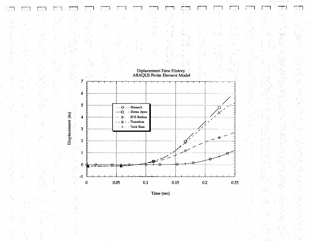
c! 0
0
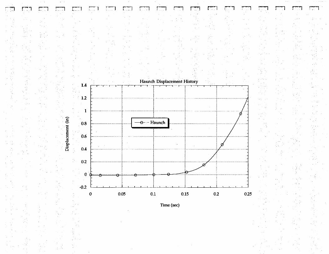
F-
I i ........... t
...........
...........
Lu \
...........................
............ < ..............
-
... ...... .(..
....
...........................
A .!"
i ............
.........
\
.............
.............
............
................
1 .......... I
............
............
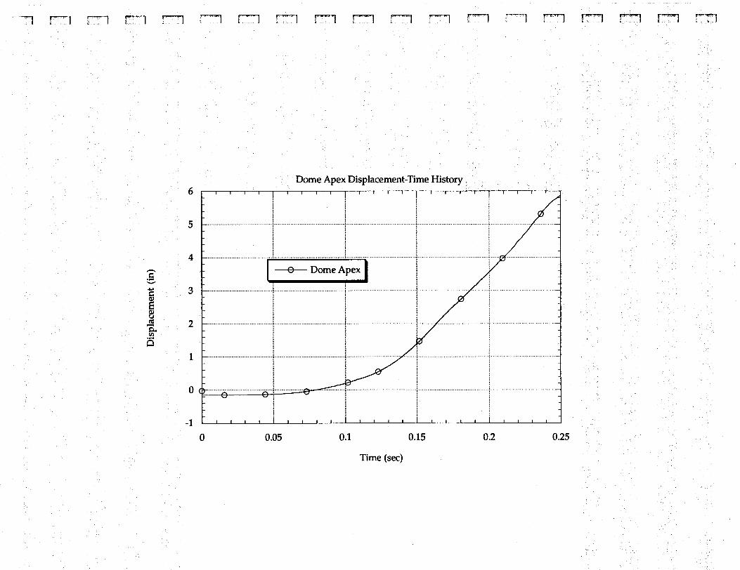
r
i E. f
Et
1.1 t t..- ........
c
I.. .
"\ ...............................
.............
"\ ..............
.............
.............
..............
\
..............
..............
r
................
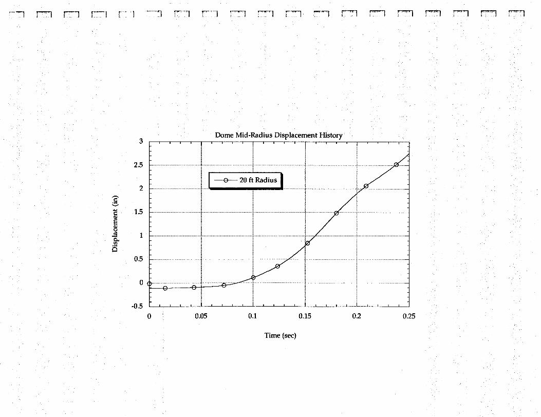
In
T! 0
T! 0
In
8 0
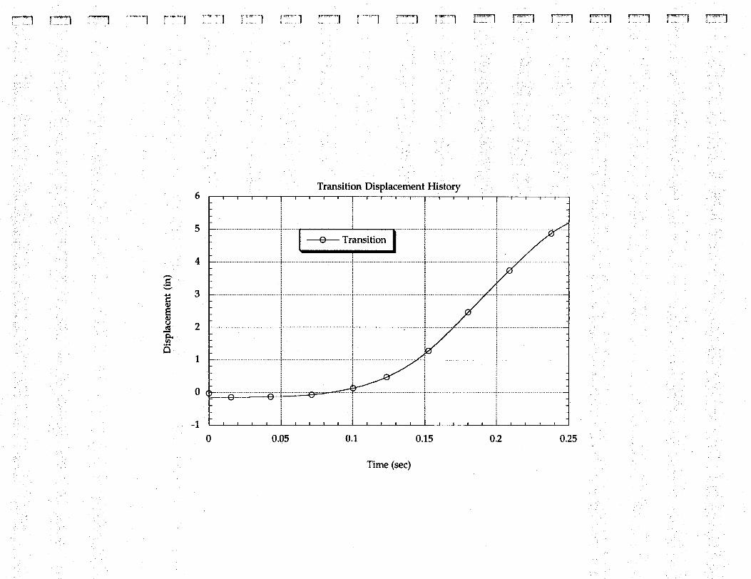
t \ ,:
.............................
.............. y ...............
...................
.............. - ...............
A \
.............
.............
.............
..............
\
...............
............... ..............
..............
I, ........... ..............
1 I
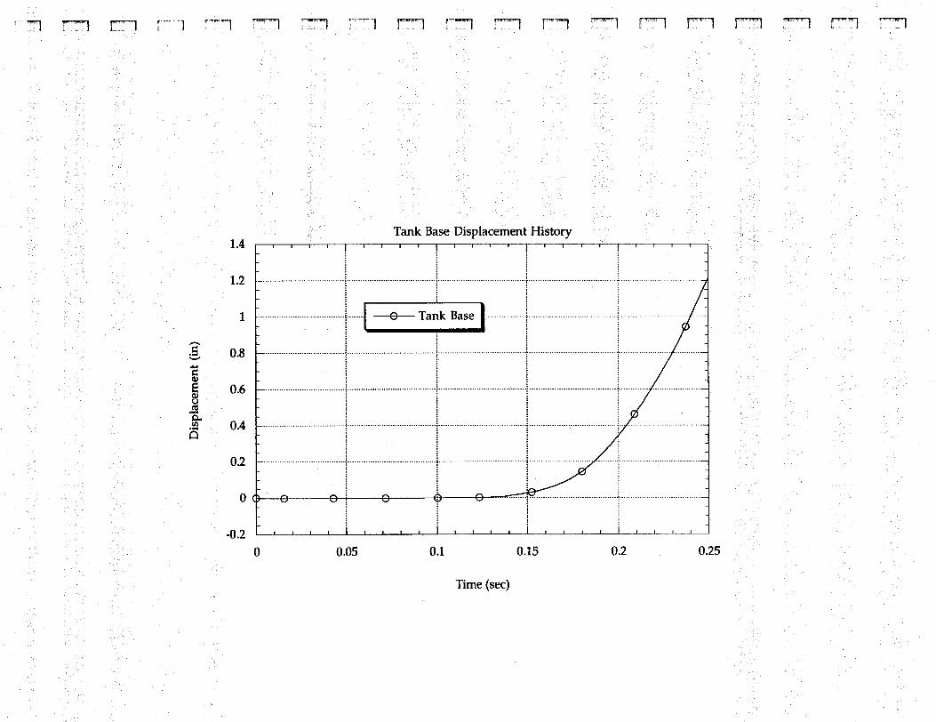
r
i. ...........
............. : ...............
...... ......-. ............ \
............
............
............
r? 0
0
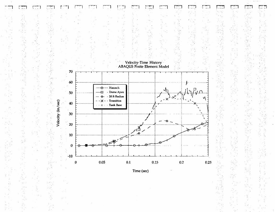
t c
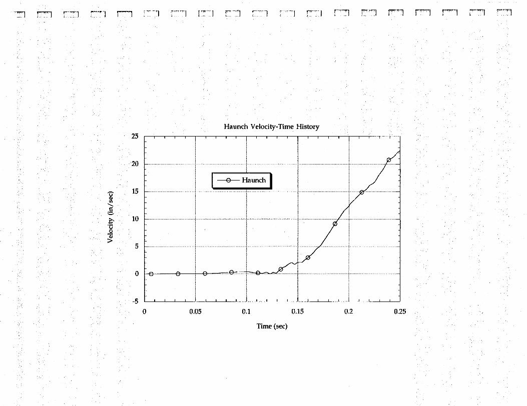
t ..........................................................
~,
,,
11
~ 1
................
1 (
................ I c ....
.... .... ;r [ I) ....
0
0
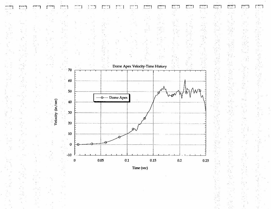
@!
0
T! 0
0
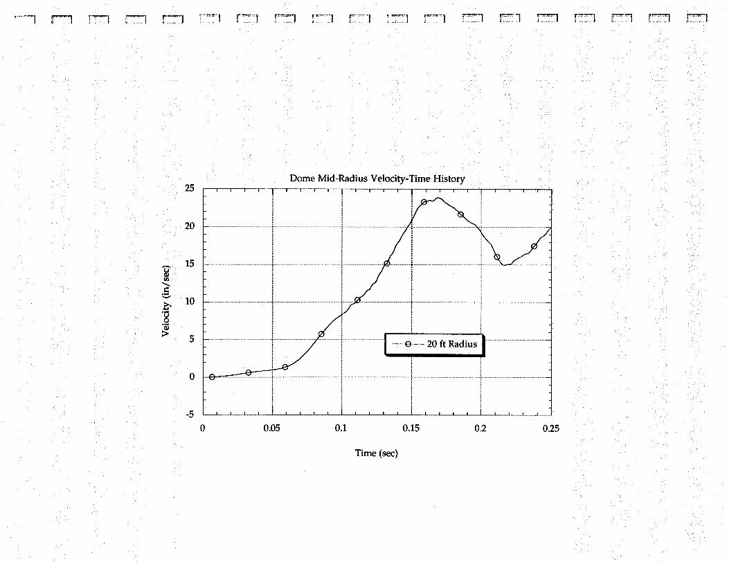
/” ........................................
.....
i: ................. a”
L .................. < ....................
.................. < ....................
.............
\.. .....................................
....
.(..
....
.,.. lj
I
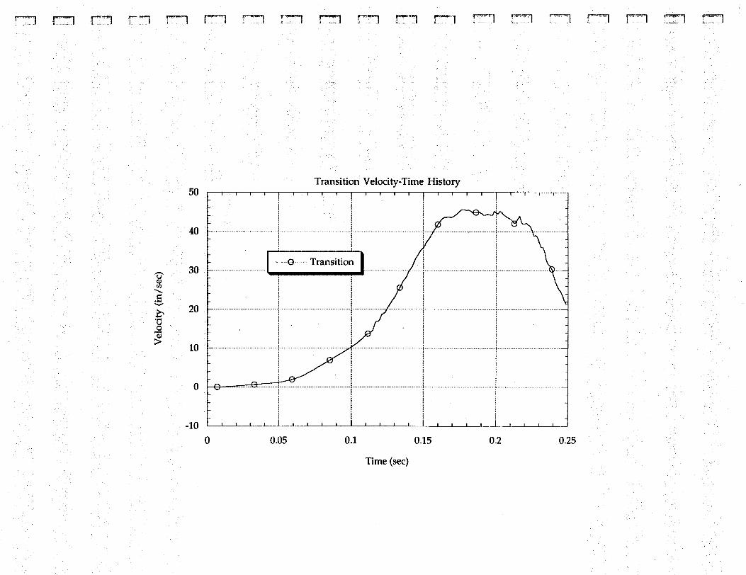
c t- ...............
I-
T
T
1
................. .... .....
i ................
................ 1 v1
0
hl
............... cu 0
m
T! 0
............... 1 h
V
m 0
) Y
z i= ............... la
...............
~
10
8 0
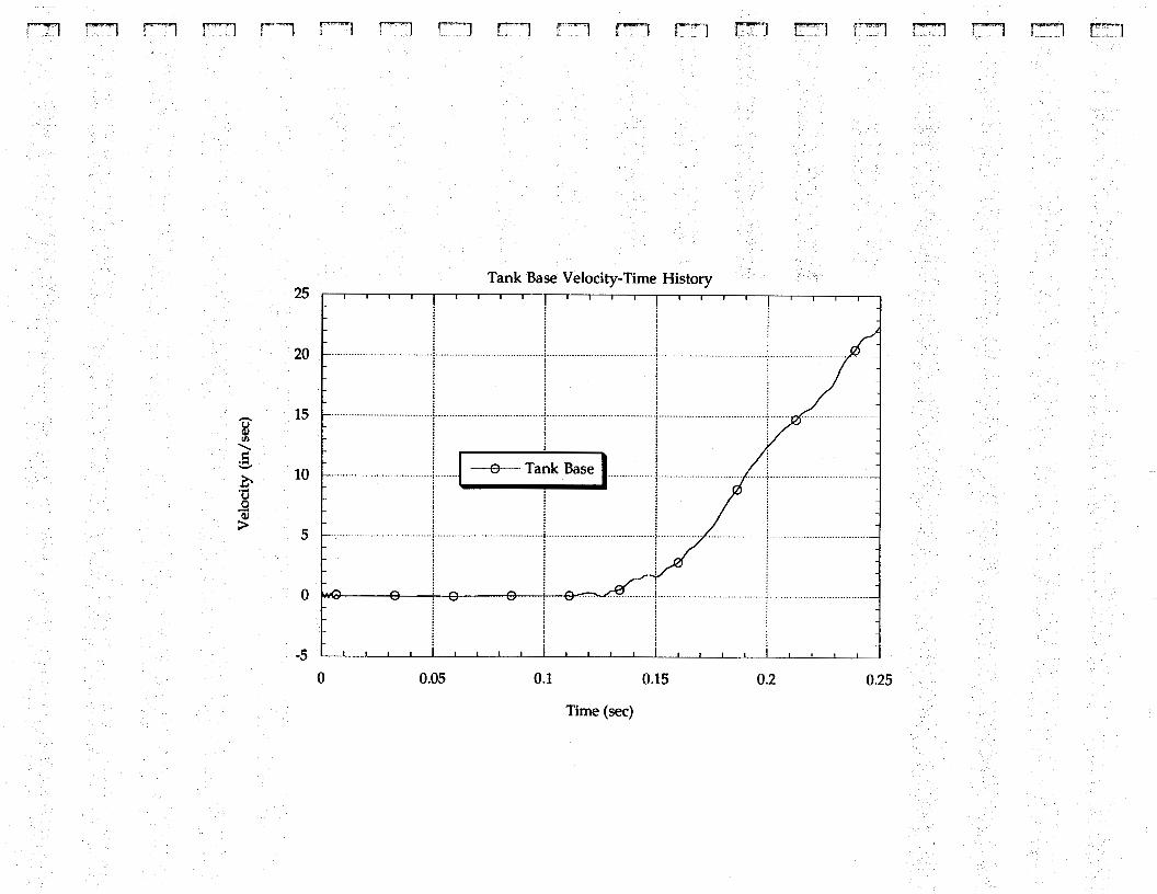
c L ...............
rn
.................
.................
.................
.................
................ i
........
.... .^_
................... ia