Comparison Between Equations Obtained by Means of …cdn.intechopen.com/pdfs-wm/40277.pdf · Comparison Between Equations Ob tained by Means of Multiple Linear Regression and Geneti

3,350+OPEN ACCESS BOOKS

108,000+INTERNATIONAL

AUTHORS AND EDITORS115+ MILLION

DOWNLOADS

BOOKSDELIVERED TO

151 COUNTRIES

AUTHORS AMONG

TOP 1%MOST CITED SCIENTIST

12.2%AUTHORS AND EDITORS

FROM TOP 500 UNIVERSITIES

Selection of our books indexed in theBook Citation Index in Web of Science™

Core Collection (BKCI)

Chapter from the book Genetic Programming - New Approaches and SuccessfulApplicationsDownloaded from: http://www.intechopen.com/books/genetic-programming-new-approaches-and-successful-applications

PUBLISHED BY

World's largest Science,Technology & Medicine

Open Access book publisher

Interested in publishing with IntechOpen?Contact us at [email protected]

http://www.intechopen.com/books/genetic-programming-new-approaches-and-successful-applications

mailto:[email protected]

Chapter 11

© 2012 Arganis et al., licensee InTech. This is an open access chapter distributed under the terms of the Creative Commons Attribution License (http://creativecommons.org/licenses/by/3.0), which permits unrestricted use, distribution, and reproduction in any medium, provided the original work is properly cited.

Comparison Between Equations Obtained by Means of Multiple Linear Regression and Genetic Programming to Approach Measured Climatic Data in a River

M.L. Arganis, R. Val, R. Domínguez, K. Rodríguez, J. Dolz and J.M. Eaton

Additional information is available at the end of the chapter

http://dx.doi.org/10.5772/50556

1. Introduction

The Ebro River is located in north-eastern Spain. After crossing the Catalan coastal mountain system, the Ebro reaches the sea. Along the lower part of the river, about 100 km from the mouth, there is a system of three reservoirs: Mequinenza (1500 hm3), Ribarroja (210 hm3) and Flix (11 hm3). These reservoirs regulate the hydrologic regime of the lower part of the river until it reaches the sea. The Mequinenza and Ribarroja reservoirs were finished in the late 1960s (in 1966 and 1969, respectively), while the Flix reservoir was completed in 1945. About 5 km downstream from the Flix reservoir is the Ascó nuclear power plant, which began its activity in December 1984 [1].

Ascó Nuclear Power Station, located on the Ebro River in Spain (Figure 1), takes river water for cooling purposes. The temperature of discharged water must be less than 13 ºC, however five kilometers downstream a water temperature of nearly 14ºC was estimated and such an anomaly was reported to the nuclear center. A detailed analysis shows the relationship between water temperature variation and the presence of a cascade dam system upstream of the Ascó Nuclear Power Station. Water temperature decreases downstream in the outlets of cascade dam systems [1]. During the winter period there also exists thermal stratification within the river, whereby water temperatures near deep intake areas are considerably less than the ambient temperature. Such a situation impacts water taken for cooling purposes by Ascó Nuclear Power Station.

Throughout the years, the human being has made use of fluvial ecosystems. Some actions have caused changes in the thermal regimes of rivers (eg. [2 ,3]).

Genetic Programming – New Approaches and Successful Applications 240

Reservoirs and the use of water for cooling are the most important sources of water temperature modifications caused by humans. The use of water for cooling, usually by power plants, causes the water to become warmer [4]. This is often called “thermal pollution”.

Reservoirs can cause various effects, depending on various factors such as the climate, the size of the impoundment, the residence time, the stability of the thermal stratification and the depth of the outlet [5]. Due to thermal stratification occurs, the water from deep-release reservoirs is cooler in the summer and warmer in the winter than it would be without the reservoir [6,7]. Water diversions can also alter water temperature regimes because they reduce discharge, which causes water temperature range to increase throughout the year [8]. Irrigation is also known to decrease discharge and increase water temperature [9].

In order to preserve the ecological balance it is very important to have a continuous inspection of water quality in that portion of the river. Freshwater organisms are mostly ectotherms and are therefore largely influenced by water temperature. Some of the expected consequences of a water temperature increase are life-cycle changes [4, 10], and shifts in the distribution of species with the arrival of allochthonous species [11, 12] and the expansion of epidemic diseases [13] as a possible result. Also, aquatic flora and fauna depend on dissolved oxygen to survive and this water quality parameter is a function of water temperature as well.

Water temperature variation analysis, in a river with a cascade dam, involves several hydrological and environmental aspects because of the dams impact on aquatic flora and fauna as shown by [14,15,16,1,17,18,19].

Because temperature is a water quality parameter that affects aquatic flora and fauna, it is important to have mathematical models which allow one to make estimations of water temperature behavior. These models are based on climatic data such as solar radiation, net radiation, relative humidity, air temperature, and wind speed. Accurate water temperature modeling may help diminish the environmental impact of increased water temperature on aquatic flora and fauna within the river.

Genetic programming (GP) algorithms have been used to derive equations which estimate the ten minute average water temperature from known variables such as relative humidity, air temperature, wind speed, solar radiation, and net radiation [20]. Only air temperature and relative humidity were associated with water temperature in some of the resulting equations, even though solar radiation is known to increase water temperature in rivers and ponds.

A correlation analysis could prove the implicit participation of solar radiation as a variable in air temperature, even though an explicit solar radiation term does not appears in the equation. Solar radiation was assumed to be independent with respect to water temperature resulting from neglecting the lag time between a change in the solar radiation value and the corresponding change in water temperature, [1] estimated this lag time to be nearly 160 minutes. By inputting data to both the genetic programming algorithm and multiple linear

Comparison Between Equations Obtained by Means of Multiple Linear Regression and Genetic Programming to Approach Measured Climatic Data in a River 241

regression (MLR) in this study, it was possible to identify the relative significance of each climatic variable in estimating water temperature.

Tests were made from data collected at the Ribarroja Station, which is located on the Ebro River in Spain (Figure 1).

Figure 1. Location of reservoirs and climatic stations on the Ebro River in Spain (Val, 2003 and google.com.mx)

2. Methods

2.1. Genetic programming

Evolutionary Computation (EC) are learning, search and optimization algorithms based on the theories of natural evolution and genetic. The steps of the basic structure of this kind of algorithms are shown in Figure. First, an initial population of potential solutions is randomly created (in the case of a Simple Genetic Algorithm (SGA), the initial population is composed of binary individuals). Then, the individuals of this population are evaluated considering the problem to be solved (environment) where a fitness value is assigned to each individual depending on how close individuals are to the optimum. A new generation is created by selecting the fitter solutions of previous generation and then, genetic operators such as crossover and mutation (Alter P(t) of Figure 2) are applied to selected individuals in order to create a new population (offsprings) which improve their fitness values in comparison to previous generation. This new population is evaluated and selection, crossover and mutation are again applied. This process continues until a termination criterion is reached (this is commonly established as the maximum number of generation).


Genetic Programming (GP) is a class of Evolutionary Algorithm (EA) [ 21,22,23] where individuals in the population are computer programs, usually expressed as syntax trees or as corresponding expressions in prefix notation (see Figure 3).

Figure 2. Evolution-based algorithm.

Figure 3. Genetic programming representation: syntax tree, LISP or prefix notation, mathematical function and MATLAB program


As seen from Figure 3, individuals are created based on a function and terminal set according to the problem to be solved. A root node is generally a function selected randomly from the function set. Then, functions and terminals are chosen in order to form the syntax tree that represents an individual. It is important to set a maximum depth or maximum number of nodes, thus the size of the individuals can be control and avoid bloating. Bloat is the rapid growth of programs produced by genetic programming or variable coding heuristics.

The fitness value of the population is usually calculated by running each individual with the problem input data, or testing data, and see how close the output of the program (individual) is to some desired (reference) output specified by the user.

Each generation, fitter individuals are evolved by means of crossover and mutation. Crossover is a sexual genetic operator that takes two parent-individuals, randomly selects a node in each parent and exchanges the associated sub-branch starting from the selected node between the parents producing two new individuals. Due to GP uses variables individuals representation, the selected nodes for crossing over two individuals are different in each parent. Note that if the parents to crossover are identical, the new two offsprings are generally different to the parents because the node selected for crossing over is different in each paren. In contrast to Genetic Algorithms, when two identical parents are crossing over, the offsprings are similar to their parents because the crossing point is the same for both parents and they have the same length.

Mutation is a asexual genetic operator that takes an individual, randomly selects a node and replaces the associated branch for a new branch generated based on the primitive set (functions and terminals sets).

The application of evolutionary computing algorithms has expanded in the last few years to several engineering applications, particularly in regards to hydraulics and hydrological engineering. Examples include: studies of hydroinformatics by [24,25]; studies in rainfall runoff modeling by [26-31] . The unit hydrograph for a typical urban basin was obtained by means of genetic programming in [32].

A study of Chezy’s roughness coefficient by [33], who also uses an evolutionary polynomial regression in [34,35].

A deep percolation model using genetic programming was obtained by [36]. Models related to sediments were obtained with genetic programming by [37].

Evapotranspiration phenomena has been predicted by means of genetic programming [38]. The flood routing problem was analyzed by means of genetic programming by [39] and the soil moisture too [40].

In this work, a genetic programming algorithm operating in the MATLAB environment [41] developed at the Instituto de Investigaciones en Matemáticas Aplicadas y en Sistemas (IIMAS), Universidad Nacional Autónoma de México (UNAM) was applied and compared with a traditional curve adjustment technique, in an attempt to get another useful application of these


optimization procedures. Here, a stochastic universal selection method was used [42] (Baker, 1987); crossover operator was used with a probability of 90% (see Table 1). It is important to mention that two different mutation operators were used. The first one with a probability of 5% randomly selects a branch and then it exchanges this selected branch by a new generated one. The second mutation operator works by selecting constant values and with a probability of 5%, these constants are mutated by adding a random value of a defined range.

This climatic data modeling problem is expressed as a symbolic regression, a common application of genetic programming, where function set consists of arithmetic and trigonometric functions and terminals set consists of climatological variables which are described in next section.

2.2. Input data

Water temperature (Tw), solar radiation (rs), net radiation (rn), relative humidity (hr), air temperature (Ta), and wind speed (Vv) data measured at the Ribarroja Station from January to June of 1998 were utilized in this study. The ten minute water temperature average was calculated using all of these variables. Later, the averaged air temperature and relative humidity (in decimals) were filtered to take into account a seven day relay. Data filtering was done with the following equation:

1t

t k

ii t

f

VVi

k

−

==+

(1)

Where :

Vi is the original independent variable

tfVi is the filtered independent variable and

k is the size or widow filter (in this case k=6).

Recorded solar radiation at minute ti has its influence on water temperature at instant ti+160 [1] and such a gap needs to be taken into account for all considered data. For example, the first data point of the dependent variable, ten minute average water temperature at instant ti+160, was coupled with the first data point of the independent variable, such as solar radiation at instant ti. For the independent variables, net radiation (rn) and wind speed (vw) values of ti+160 were used, while air temperature and relative humidity values were considered using both seven day filtering and values corresponding to instant ti+160 .

2.3. Objective function

The objective function was to minimize the mean square error between the calculated and measured data using the following equation:

21 ˆmin ( )nZ Tw Twn

= − (2)


Where:

Z is the function to minimize Tw is the average of measured temperature each ten minute interval in ºC T̂w is the calculated temperature with the genetic programming algorithm in ºC, and n is the data number.

2.4. Parameter setting

Parameters used in the genetic programming algorithm are shown in Table 1. MaxNumNodes corresponds to the maximum number of nodes an individual can have; meanwhile MaxNodesMut represents the maximum number of nodes a new created branch can have for mutation. Terminal set represents the independent variables and Tw corresponds to the dependent variable to be modeled.

Parameter Value Description

Pcross 0.9 Probability of crossover

Pmut 0.05 Probability of mutation

Pmut_R 0.05 Probability of mutating a node containing a constant

MaxNodesMut 8 Maximum number of nodes for mutation

Nind 200 Number of individuals in the population

MaxNumNodes 30 Maximum number of nodes for each individual

MaxGen 5000 Maximum number of generations (iterations)

Function_Set +,-,*, /,cos Function set

Terminal Set rs, rn, hr, Ta, Vv Climatological variables

Table 1. Parameter settings

The function cosine (cos) was included in the function set due to preliminary tests, where a reduction in mean quadratic error was obtained, included this cosine function. This fact is related to one of the two properties that GP individuals must satisfy: sufficiency. This property says that the set of terminals and the set of functions should be defined in order to express a solution to the study problem [23]. The second property, closure, specifies that each of the functions in the function set can be able to accept, as its argument, any value and data type that may possibly be returned by any function and any value or data type that can be possibly assumed by any terminal [23]. In this approach, a protected division was implemented in order to avoid a division by zero. In this situation occurs, a high value is returned.

By including the cosine function, associated equation also presented a good reproduction of the periodic behavior of water temperature over time.


2.5. Multiple linear regressions

Multiple linear regressions (MLR) relate a dependent variable, y, with two or more independents variables, x1, x2, x3,…, xn, by means of an equation expressed as:

1 1 2 2 3 3 n ny a x a x a x a x= + + + + (3)

Coefficients a1,a2,a3,…an, are weighting factors which allow one to see the relative importance of each variable xi as y is approached. Indirectly the coefficients can indicate if there is a strong correlation or lack of correlation between xi and y.

This method is often applied for several hydrology problems such as: forecasting equations for standardized runoff in a region of a country with standardized teleconnection indices, when El Niño or La Niña phenomenon occur [43] (González et al., 2000), or as an auxiliary method in estimating intensity-duration-frequency curves. In this research, regressions were made using the Microsoft Excel data analysis tool.

3. Results and discussion

Measured climatic data of the above variables, corresponding from January to June of 1998, were fed into both the symbolic regression genetic programming model and the multiple linear regression model in order to estimate water temperature. The models were then applied using data from January to June of 1999 in order to approach water temperature averages. Comparisons for the1998 and 1999 results were then made.

The genetic programming algorithm (equation 4) determined the next mathematical model which approaches the water temperature (average of each ten minutes).

( cos(cos(( cos ) * 0.6904149))

cos(cos(1.17748531* cosh )) 1.87808843) * 0.67508628w a a a

a r

T T T TT

= + + ++ + +

(4)

Using equation (4), the individual with the best performance reported an objective function value of 0.7922.

Meanwhile, the multiple linear regression model is expressed as follows:

w s n a v rT 0.00022505r 0.00036289r 0.66464617T 0.02807297V 1.24438982h 3.87792166= + + − − + (5)

Where:

Tw corresponds to the average water temperature each ten minute interval at instant t+160 in ºC Ta is the average air temperature each ten minute interval, with seven days filtering, corresponding to instant t+160, in ºC hr represents the average relative humidity each ten minutes interval, with seven days filtering, corresponding to instant t+160 in decimals


rs is the average solar radiation each ten minutes interval, at instant t, in W/m2

rn corresponds to the average net radiation each ten minutes interval, corresponding to instant t+160, in W/m2

and finally,

vv represents the average wind speed each ten minutes interval, corresponding to instant t+160, in m/s.

The objective function value using equation 5 was 0.8724.

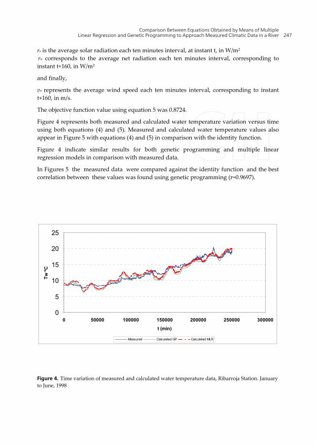
Figure 4 represents both measured and calculated water temperature variation versus time using both equations (4) and (5). Measured and calculated water temperature values also appear in Figure 5 with equations (4) and (5) in comparison with the identity function.

Figure 4 indicate similar results for both genetic programming and multiple linear regression models in comparison with measured data.

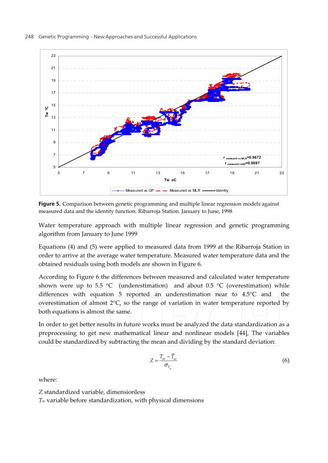
In Figures 5 the measured data were compared against the identity function and the best correlation between these values was found using genetic programming (r=0.9697).

Figure 4. Time variation of measured and calculated water temperature data, Ribarroja Station. January to June, 1998

0

5

10

15

20

25

0 50000 100000 150000 200000 250000 300000

t (min)

Tw

ºC

Measured Calculated GP Calculated MLR


Figure 5. Comparison between genetic programming and multiple linear regression models against measured data and the identity function. Ribarroja Station. January to June, 1998

Water temperature approach with multiple linear regression and genetic programming algorithm from January to June 1999

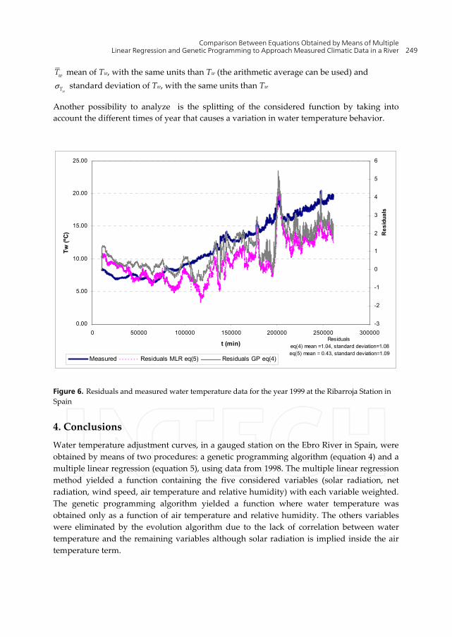
Equations (4) and (5) were applied to measured data from 1999 at the Ribarroja Station in order to arrive at the average water temperature. Measured water temperature data and the obtained residuals using both models are shown in Figure 6.

According to Figure 6 the differences between measured and calculated water temperature shown were up to 5.5 °C (underestimation) and about 0.5 °C (overestimation) while differences with equation 5 reported an underestimation near to 4.5°C and the overestimation of almost 2°C, so the range of variation in water temperature reported by both equations is almost the same.

In order to get better results in future works must be analyzed the data standardization as a preprocessing to get new mathematical linear and nonlinear models [44], The variables could be standardized by subtracting the mean and dividing by the standard deviation:

w

w w

T

T TZ

σ−

= (6)

where:

Z standardized variable, dimensionless Tw variable before standardization, with physical dimensions

5

7

9

11

13

15

17

19

21

23

5 7 9 11 13 15 17 19 21 23

Tw oC

Tw

ºC

Measured vs GP Measured vs MLR Identity

r measuerd vs MLR=0.9672

r measuerd vsGP=0.9697


wT mean of Tw, with the same units than Tw (the arithmetic average can be used) and

wTσ standard deviation of Tw, with the same units than Tw

Another possibility to analyze is the splitting of the considered function by taking into account the different times of year that causes a variation in water temperature behavior.

Figure 6. Residuals and measured water temperature data for the year 1999 at the Ribarroja Station in Spain

4. Conclusions

Water temperature adjustment curves, in a gauged station on the Ebro River in Spain, were obtained by means of two procedures: a genetic programming algorithm (equation 4) and a multiple linear regression (equation 5), using data from 1998. The multiple linear regression method yielded a function containing the five considered variables (solar radiation, net radiation, wind speed, air temperature and relative humidity) with each variable weighted. The genetic programming algorithm yielded a function where water temperature was obtained only as a function of air temperature and relative humidity. The others variables were eliminated by the evolution algorithm due to the lack of correlation between water temperature and the remaining variables although solar radiation is implied inside the air temperature term.

0.00

5.00

10.00

15.00

20.00

25.00

0 50000 100000 150000 200000 250000 300000

t (min)

Tw

(ºC

)

-3

-2

-1

0

1

2

3

4

5

6

Re

sid

ua

ls

Measured Residuals MLR eq(5) Residuals GP eq(4)

Residuals eq(4) mean =1.04, standard deviation=1.08 eq(5) mean = 0.43, standard deviation=1.09


Comparing measured data with calculated data, for the year 1998, led to only minor errors in estimating the average water temperature using the genetic programming algorithm. When equations (4) and (5) were applied to another year, 1999, minor mean quadratic error in estimating water temperature was obtained using the multiple linear regression equation (5). The mean quadratic error associated with the multiple linear regression equation (5) for 1999 was 1.375 ºC; whereas with the genetic programming equation (4) was 2.248 ºC. This error can be considered acceptable if one takes in account the average temperature from January to June 1998 was 12.54 ºC, whereas the average temperature in 1999 for the same period was 11.62 ºC. The residuals obtained with equations (4) and (5) using data for the year 1999 had average values of 1.04 ºC and 0.43 ºC, respectively and with this criteria, multiple linear regression model can be considered better than the GP. However, reviewing the standard deviations, both models had almost the same value (1.09 ºC and 1.08 ºC, respectively).

The described procedures are then useful because equations similar to (4) or (5) can estimate important water quality characteristics, such as water temperature, using previously measured climatic data, predicted climatic data, and hydrological parameters for a given time period.

Engineer’s criteria and common sense must be considered before to apply any model to simulate physical variables.

Some standardization procedures to the involved data are suggested in order to improve the results from new models that can be obtained.

The methods here applied are undoubtedly useful in several areas of knowledge, and can led us to new approaches to physical phenomena by considering measured field data.

Future work is focuses on the use of NARMAX (Non-linear Autorregressive Moving Average with eXogenous inputs) model combined with genetic programming in order to model the water temperature providing more accurate equations.

Author details

M.L. Arganis and R. Domínguez PUMAGUA, Universidad Nacional Autónoma de México, México

R. Val and K. Rodríguez Instituto de Investigaciones en Matemáticas Aplicadas y en Sistemas, Coyoacán, D.F. México

Josep Dolz Universidad Politécnica de Cataluña, Barcelona, España

J.M. Eaton Centre for Hydrology, Micrometeorology and Climate Change, Department of Civil and Environmental Engineering, University College Cork, Cork, Republic of Ireland


Acknowledgements

Authors gratefully acknowledge the financial support under the project PAPIIT no. IN109011.

5. References

[1] [1] 23. Val S R (2003) Incidencia de los embalses en el comportamiento térmico del río. Caso del sistema de embalses Mequinenza-Ribarroja-Flix en el Río Ebro. Tesis Doctoral. Universidad Politécnica de Catalunya. Barcelona, España.

[2] Alberto F, Arrúe JL (1986) Anomalías térmicas en algunos tramos de la red hidrográfica del Ebro. Anales de la Estación Experimental Aula Dei 18: 91-113.

[3] Preece RM, Jones HA ( 2002) The effect of Keepit Dam on the temperature regime of the Namoi River, Australia. River Research and Applications 18: 397-414. DOI: 10.1002/rra.686

[4] Hellawell JM (1986) Biological indicators of freshwater pollution and environment management. Elsevier, London. 546 pp.

[5] Lessard JL, Hayes DB (2003) Effects of elevated water temperature on fish and macroinvertebrate communities below small dams. River Research and Applications 19: 721-732. DOI: 10.1002/rra.713

[6] Ward JV (1985) Thermal characteristics of running waters. Hydrobiologia 125: 31-46.

[7] Webb BW, Walling DE (1993) Temporal variability in the impact of river regulation on thermal regime and some biological implications. Freshwater Biology 29: 167-182.

[8] Meier W, Bonjour C, Wüest A, Reichert P (2003) Modeling the effect of water diversion on the temperature of mountain streams. Journal of Environmental Engineering 129: 755-764. DOI: 10.1061/(ASCE)0733-9372(2003)129:8(755)

[9] Verma RD (1986) Environmental impacts of irrigation projects. Journal of Irrigation and Drainage Engineering 112: 322-330.

[10] Winfield, IJ, Nelson JS (1991) Cyprinid fishes. Systematics, biology and exploitation. Chapman & Hall, London. 667 pp.

[11] Schindler, DW (1997) Widespread effects of climatic warming on freshwater ecosystems in North America. Hydrological Processes, 11: 1043-1067.

[12] [12] Walther, Gr, Post E, Convey P, Menzel A., Parmesan C, Beebee TJC, Fromentin JM, Hoegh-Guldberg O,. Bairlein F (2002) Ecological responses to recent climate change. Nature, 416: 389-395.

[13] Harvell, CD, C. E Mitchell, J. R Ward, S. Altizer, A. P Dobson, R. S. Ostfeld & M. D. Samuel. 2002. Climate warming and disease risks for terrestrial and marine biota. Science, 296: 2158-2162.


[14] Smalley DH, Novak JK (1978). Natural thermal phenomena associated with reservoirs. In Environmental Effect of Large Dams. ASCE.

[15] [15]. Cassidy RA (1989). Water temperature, dissolved oxygen and turbidity control in reservoir releases. In: Alternatives in Regulated River Management.

[16] Mohseni O, Stefan HG (1999). Stream temperature/air temperature relationship: A physical interpretation. Journal of Hydrology 218: 128–141.

[17] Caissie D, El-Jabi N, Satish MG (2001). Modeling of maximum daily water temperature in a small stream using air temperature. Journal of Hydrology 251: 14-28.

[18] Batalla RJ, Gómez CM, Kondolf GM (2004). Reservoir-induced hydrological changes in the Ebro River basin (NE Spain). Journal of Hydrology 290: 117–136.

[19] Morrill JC, Bales RC, Conklin MH (2005). Estimating stream temperature from air temperature: Implications for future water quality. Journal of Environmental Engineering.131: 139-146.

[20] 1. Arganis ML, Val SR, Rodríguez VK, Domínguez MR, Dolz R.J (2005). Comparación de curvas de ajuste a la Temperatura del Agua de un río usando programación genética. Congreso Mexicano de Computación Evolutiva COMCEV.

[21] Cramer NL (1985). A representation for the adaptive generation of simple sequential programs. In Proceedings of International Conference on Genetic Algorithms and the Applications: 183-187.

[22] Koza JR (1989). Hierarchical genetic algorithms operating on populations of computer programs. In Proceeding of the 11th International Joint Conference on Artificial Intelligence. 1: 768-774.

[23] Koza JR (1992) Genetic Programming: On the Programming of Computers by Means of Natural Selection. MIT Press.

[24] Babovic V, Keijzer M (2000). Genetic programming as a model induction engine. Journal of Hydroinformatics 2: 35-60.

[25] [25] Babovic V, Keijzer M, Rodríguez AD, Harrington J (2001). An evolutionary approach to knowledge induction: Genetic programming in Hydraulic Engineering. Proceedings of the World Water & Environmental Resources Congress, May 21-24.

[26] Savic DA, Walters GA, Davidson JW (1999). A Genetic Programming Approach to Rainfall-Runoff Modeling. Water Resources Management 13: 219–231.

[27] Drécourt JP, Madsen H (2001). Role of domain knowledge in data-driven modeling. 4th DHI Software Conference & DHI Software Courses Helsingør, Denmark, June 6-13.

[28] [28]Whigham PA, Crapper PF (2001). Modeling Rainfall-Runoff using Genetic Prograaming. Mathematical and Computer Modeling. 33: 707-721.

[29] Khu ST, Keedwell EC, Pollard O (2004). An evolutionary-based real-time updating technique for an operational rainfall-runoff forecasting model, In: Complexity and Integrated Resources Management, Trans. In Proceedings of the 2nd Biennial Meeting of the International Environmental Modelling and Software Society. 1: 141–146.


[30] Khu ST, Liong SY, Babovic V, Madsen H, Muttil N (2001). Genetic programming and its application in real time runoff forecasting.Journal of the American Water Resources Association. 37: 439-451.

[31] Dorado J, Rabuñal JR, Puertas J, Santos A, Rivero D (2002). Prediction and modeling of the flow of a typical urban basin through genetic programming. Applications of Evolutionary Computing. 190-201

[32] Rabuñal JR, Puertas J, Suárez J, Rivero D (2007). Determination of the unit hydrograph of a typical urban basin using genetic programming and artificial neural networks. Hydrological processes. 21: 476–485.

[33] Giustolisi O (2004). Using genetic programming to determine Chezy resistance coefficient in corrugated channels. Journal of Hydroinformatics. 6: 157-173.

[34] Giustolisi O, Doglioni A, Savic DA, Webb B (2004). A Multimodel Approach to Analysis of Environmental Phenomena. Web site: http://www.iemss.org/iemss2004/pdf /evocomp/giusamul.pdf

[35] Giustolisi O, Doglioni A, Savic DA, Webb B (2007). A multimodel approach to analysis of environmental phenomena, Environmental Modelling and Software. 22: 674-682.

[36] Selle B, Muttil N (2011). Testing the structure of a hydrological model using Genetic Programming. Journal of Hydrology. 397: 1–9.

[37] Aytek A, Kisi O (2008). A genetic programming approach to suspended sediment modelling. Journal of Hydrology. 351: 288– 298.

[38] Izadifar Z, Elshorbagy A (2010). Prediction of hourly actual evapotranspiration using neural networks, genetic programming, and statistical models. Hydrological processes. 24: 3413–3425.

[39] Sivapragasam C, Maheswaran R, Venkatesh V (2008). Genetic programming approach for flood routing in natural channels. Hydrological processes. 22: 623–628.

[40] Makkeasorn A, Chang N-B, Beaman M, Wyatt C, Slater C. (2006). Soil moisture estimation in a semiarid watershed using RADARSAT-1 satellite imagery and genetic programming. Water Resources Research. 42.

[41] The MathWorks (1992). MATLAB Reference Guide. [42] Baker, J (1987). Reducing Bias And Inefficiency In The Selection Algorithm, Proc. Of

The Second International Conference On Genetic Algorithms ICGA. Grefenstette, Ed.: 14-21.

[43] González VRF, Franco V, Fuentes MGE, Arganis JML (2000). Análisis comparativo entre los escurrimientos pronosticados y registrados en 1999 en las Regiones Pacífico Noroeste, Norte, Centro, Pacífico Sur y Golfo de la República Mexicana considerando que estuvo presente el fenómeno “La Niña” y Predicción de escurrimientos en dichas regiones del país en los periodos primavera-verano y otoño-invierno de 2000. Para FIRCO. Informe Final.


[44] Arganis JML, Val SR, Prats RJ, ,Rodríguez VK, Domínguez MR, Dolz RJ (2009). "Genetic programming and standardization in water temperature modelling,” Advances in Civil Engineering. Hindawi Publishing Corporation. 2009: 10.

Documents

Comparison Between Equations Obtained by Means of …cdn.intechopen.com/pdfs-wm/40277.pdf · Comparison Between Equations Ob tained by Means of Multiple Linear Regression and Geneti