COMPARISON AMONG STRESS INTENSITY FACTOR PREDICTIONS

Antonio Carlos de Oliveira Miranda

acmiranda@unb.br

Department of Civil and Environmental Engineering, University of Brasília,

SG-12 Building, Darcy Ribeiro Campus, DF, 70.910-900, Brazil

Marco Antonio Meggiolaro

Jaime Tupiassú Pinho de Castro

meggi@puc-rio.br

jtcastro@puc-rio.br

Department of Mechanical Engineering

Pontifical Catholic University of Rio de Janeiro

Rua Marquês de São Vicente 225 – Gávea, Rio de Janeiro, RJ, 22453-900, Brazil

Luiz Fernando Martha

lfm@tecgraf.puc-rio.br

Department of Civil Engineering

Pontifical Catholic University of Rio de Janeiro

Rua Marquês de São Vicente 225 – Gávea, Rio de Janeiro, RJ, 22453-900, Brazil

Abstract. Practical steps required to obtain robust finite element triangular meshes are

evaluated, and techniques to use their predictions to calculate fatigue lives, including

load interaction effects, are discussed. Three important subjects required to implement a

complete and robust crack growth simulation are discussed here: (a) how to simulate

efficiently 2D crack paths under bi-axial loading using automatic remeshing schemes;

(b) how to choose among the various calculation methods the best one to obtain the

stress intensity factors (SIF) along the crack path; and (c) how the numerical problems

associated with excessive FE mesh refinement along the crack path may affect

predictions. Various modeling strategies are compared using different crack geometries

and mesh refinements to quantify their performance, particularly when the elements

around the crack tip are very small compared with elements in other regions. In

particular, it is shown that, contrary to many other stress analysis applications, excessive

mesh refinement may significantly degrade the calculation accuracy in crack problems.

A limit for the elements size ratio is clearly established.

Keywords: Curved crack path prediction, fatigue under complex load, stress intensity

calculation, finite element implementation.

1. INTRODUCTION

The theory required to predict the generally curved crack propagation path in two-

dimensional (2D) structural components under bi-axial loading is well known, but its

implementation in an efficient and reliable code is still far from a trivial task. The

purpose of this work is to describe how the difficulties involved in translating such

theoretical tools into practical numerical techniques have been solved, and how these

techniques were used in a successful special-purpose academic program called

Quebra2D, which means 2D fracture in Portuguese (Miranda, Meggiolaro et al. 2002;

Miranda, Meggiolaro et al. 2003). This software is an interactive graphics program for

simulating two-dimensional fracture processes based on numerical Finite Element (FE)

techniques. Additionally, three important subjects are presented to accomplish a

complete and robust simulation of fatigue crack growth (FCG): (a) how to compute

efficiently fatigue crack propagation under complex loads; (b) numerical problems that

come up when the size of FE at crack tip is very small compared to entire model; and

(c) the best method to compute SIF.

The complete automatic simulation of crack propagation in 2D using FE method

was first present by Bittencourt (Bittencourt, Wawrzynek et al. 1996) and Lim (Lim,

Johnston et al. 1996). Bittencourt used an advancing front method to create the initial

mesh and locally, in a zone near to the crack tip, in the following steps of simulation,

avoiding the remeshing of all geometry. To accomplish the simulation, three methods to

compute SIF [5-8] and also three techniques to compute the crack path were employed

(Erdogan and Sih 1963; Hussain, Pu et al. 1974; Sih 1974). Lim also used a local

method to remesh just the zone close to the crack tip to avoid the remeshing of all

geometry. In that work, four displacement-based SIF computation techniques have been

implemented (Lim, Johnston et al. 1992). Similar works have been published about the

same subject (Bouchard, Bay et al. 2000; Bouchard, Bay et al. 2003; Miranda,

Meggiolaro et al. 2003; Miranda, Meggiolaro et al. 2003; Phongthanapanich and

Dechaumphai 2004; Heintz 2006; Alshoaibi, Hadi et al. 2007; Khoei, Azadi et al. 2008;

Alegre and Cuesta 2010; Azócar, Elgueta et al. 2010; Rozumek, Lachowicz et al. 2010).

In general, these works added new mesh generation algorithms or new methods to

improve the SIF values. Only in the works of the same author (Miranda, Meggiolaro et

al. 2003; Miranda, Meggiolaro et al. 2003), the FCG under complex loads is present by

using an unbound global-local approach. In general, the other works, the FCG is

computed under constant load with Paris equation (Paris, M.P. Gomez et al. 1961),

which is incomplete because only represents a part of crack growth rate of material.

Most works lack of sufficient information to create an environment to compute

efficiently FCG.

Note that this work does not intend to re-analyze the advantages and disadvantages

of using FE in computational fracture mechanics, neither to compare FE with other

approaches. This task has been recently addressed by Ingraffea (Ingraffea 2004), who

studied the taxonomy of the methods used to represent cracks in a numerical model, and

the fundamental differences between them. Details about the historical development of

computational fracture mechanics are not discussed here either, as they can be obtained

in Ingraffea (Ingraffea and Wawrzynek 2003) and Sinclair (Sinclair 2004) , for instance.

In the following sections, a brief description of practical steps required to implement

a robust but efficient auto-adaptative FE mesh are described. Important details required

for the automation of the crack growth numerical predictions under complex loads are

discussed. Based on 864 FE calculations, a section compares SIF predictions and their

effects when the size of crack is decrease.

2. FINITE ELEMENT MESH GENERATION

This section describes the strategies adopted in Quebra2D (Miranda, Meggiolaro et

al. 2002; Miranda, Meggiolaro et al. 2003) to obtain triangular meshes in domains.

More details about this piece of software will be described in the next section. The

meshing algorithm works both for regions without cracks or with one or multiple

cracks, which may be either embedded or surface breaking (Miranda, Cavalcante Neto

et al. 1999). This is an adaptation of an algorithm previously proposed for generating

unstructured meshes for arbitrarily shaped three-dimensional regions (Cavalcante Neto,

Wawrzynek et al. 2001) and the same strategy was adopted for surface mesh generation

(Miranda, Martha et al. 2009). The algorithm has been designed to meet four specific

requirements, as follows.

First, the algorithm should produce well-shaped elements, avoiding elements with

poor aspect ratio. Second, the generated mesh should conform to an existing

discretization on the region boundary. This is important to simulate crack growth,

because it allows local remeshing in a region near a growing crack. Third, the algorithm

should transit smoothly between regions with elements of highly varying size, because

in crack analysis it is not uncommon for the elements near the crack tip to be two or

even three orders of magnitude smaller than the other elements. Fourth, the algorithm

should have specific capabilities for modeling cracks, which are usually idealized

without volume.

The meshing algorithm incorporates well-known meshing procedures (Lo 1985;

Lohner and Parikh 1988; Peraire, Peiro et al. 1988; Jin and Tanner 1993; Moller and

Hansbo 1995; Chan and Anastasiou 1997; Rassineux 1998) and introduces a few

original steps. It includes an advancing front technique along with a “background”

structure to develop local guidelines for the size of the generated elements. It takes

special care to generate elements with the best possible shape for each new crack front

while it advances. Such “advance front” algorithm is described in detail in (Lo 1985;

Miranda, Meggiolaro et al. 2003). In addition, the algorithm works with any

“background” structure.

Although many “background” structures are published in the literature as reviewed

by Quadros et al. (Quadros, Vyas et al. 2010), in the present work, as in its predecessors

(Miranda, Cavalcante Neto et al. 1999; Cavalcante Neto, Wawrzynek et al. 2001;

Miranda, Meggiolaro et al. 2003), a background quadtree structure is used to develop

local guidelines for node location in an advancing-front meshing procedure. Here, the

use of the quadtree was extended to improve local elements near the crack. The

background quadtree may potentially be adjusted to insert points to take into account

local scalar field gradients, such as in adaptive analyses or in boundary layers problems,

although this has not been addressed yet.

Basically, the background quadtree generation uses three steps (Miranda, Cavalcante

Neto et al. 1999; Cavalcante Neto, Wawrzynek et al. 2001; Miranda, Meggiolaro et al.

2003). In the first, the quadtree initialization is based on given boundary edges. Each

segment of the input boundary data is used to determine the local subdivision depth of

the quadtree. In the second step, a refinement scheme is used to force maximum cell

size. The quadtree is refined to guarantee that no cell in the mesh interior is larger than

the largest cell at its boundary. Finally, in the third step, a refinement is used to provide

minimum size disparity for adjacent cells. This additional refinement forces only one

level of tree depth between neighboring cells and provides a natural transition between

regions of different degrees of mesh refinement.

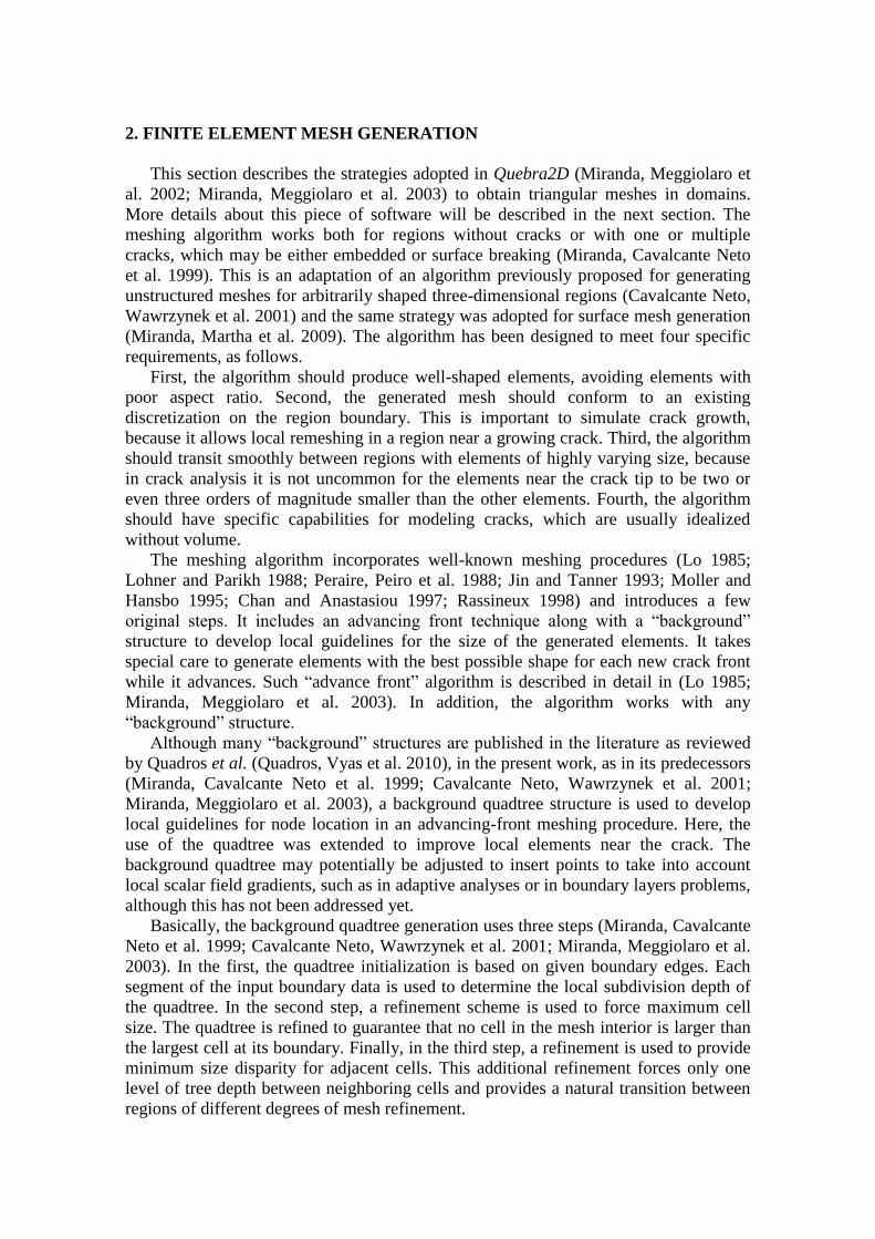
A fourth step was added here for the quadtree construction to improve local

elements near the crack. This step consists of an additional refinement to force

neighboring cells near the crack to have equal size. This step protects crack tip

elements, surrounding them with elements with the same characteristic size. This

operation is performed by specifying xy coordinates and a refinement level. Examining

the local quadtree refinement level between adjacent cells, if the difference is larger or

equal than one level, the adequate cells are refined until the specific level of refinement

is achieved. For example, Figure 1(a) shows the local quadtree generated and the

resulting mesh for a two-dimensional example without the additional refinement near

the crack tip. On the other hand, Figure 2(b) shows the local quadtree generated and the

resulting mesh after this fourth step was applied. Note the special elements around the

crack tip, which are not refined in step 4.

Figure 1 – Quadtree decomposition and resulting meshes (a) without and (b) with

additional refinement to force equal size between neighboring cells near the crack tip.

For the mesh generation algorithm, the input data is a polygonal description of the

boundary of the region to be meshed, given by a list of nodes defined by their

coordinates and a list of boundary segments (or edges) defined by their node

connectivities. This type of input can represent geometries of any shape, including holes

or cracks. From the boundary segments, the background quadtree structure is created to

control the sizes of the FE generated by the advancing front technique. The given

boundary edges form the initial front that advances as the algorithm progresses. At each

step of this meshing procedure, a new triangle is generated for each front base edge. The

front advances replacing the base edge with new triangle edges. Consequently, the

domain region is contracted, possibly into several regions. The process stops when all

the contracted regions result in single triangles.

To obtain the input data for the mesh generation algorithm in the presence of cracks,

a different procedure is applied. To insure well-shaped elements at the crack tips,

uniform rosettes of quarter-point singular elements are used for each crack tip. Then, the

boundary of the region to be meshed is the original boundary of a model which

duplicates edges along the crack faces extracting the boundary of the rosettes. Applying

the mesh generation algorithm and using the background mesh, a partial mesh is

created. Finally, the final mesh is obtained adding rosette elements into the partial mesh.

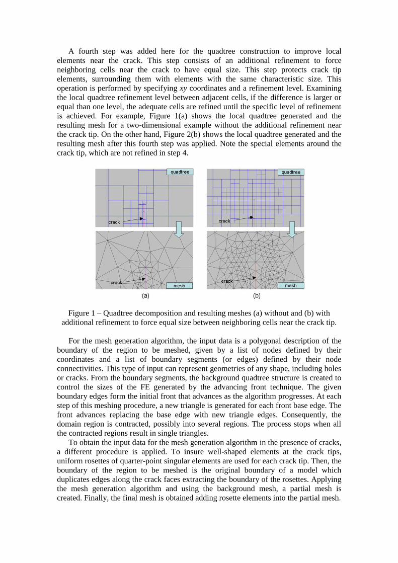
Obviously, the mesh generation algorithm will only create the final mesh if it can

deal with duplicated edges. If there are two or more nodes with the same coordinates,

which can happen in problems with closed cracks (see Figure 2), the algorithm selects

the proper node using a simple test. The test is based on the list of adjacent boundary

edges of the nodes on the advancing front. The normals to the crack curves adjacent to

the selected nodes are used to perform this test, as illustrated in Figure 2, assuming that

all crack curves are smooth (with no abrupt change in direction). In case of problems

involving crack bifurcation, specific procedures, also based on crack curve normals, are

considered.

The current algorithm may be optionally used in an adaptive mesh-generation

scheme that is based on an a priori boundary refinement, such as the scheme devised by

Paulino et al. (Paulino, Menezes et al. 1999). In this case, the adaptive process first

requires the analysis results from an initial FE mesh, usually rough, with the geometric

description, boundary conditions and its attributes. Then, a discretization of the

domain’s region boundary is performed, based on the geometric properties and

characteristic sizes of the boundary elements (adjacent to the boundary curves),

determined by the error estimation from the previous step of the FE analysis. From this

discretization, a new mesh is generated using the algorithm described above with one

minor improvement: as the quadtree structure is used to guide the size of the generated

elements, an additional quadtree refinement is performed after the initial quadtree is

generated. This additional refinement takes into account the characteristic element sizes

that are determined by the error estimation analysis.

Figure 2 – Determination of crack nodes in the advancing front procedure.

3. AUTOMATIC CRACK PROPAGATION

The automatic crack propagation strategy adopted in this work is based on a full

geometric description of the two-dimensional model. This means that there is a

geometric model that represents the structure, and the finite-element mesh is attached to

the geometric model. Analysis attributes, such as loads, support conditions and material

properties are also attached to the geometric model. The geometric description consists

of a set of curves that represent the boundaries of the regions of the model. The

boundary condition description (supports and/or loadings) is associated with the curves

and the domain parameters (such as material, properties, thickness, etc.) are associated

with the regions.

This strategy was implemented in the Quebra2D program. The crack representation

scheme used in Quebra2D is based on the discrete approach. In this sense, the program

is similar to well-known 2D simulators, such as Franc2D (Wawrzynek and Ingraffea

1987; Bittencourt, Wawrzynek et al. 1996) for instance. This program includes all

methods described above to compute the crack increment direction and the associated

stress intensity factors along the crack path. Moreover, its adaptive FE analyses are

coupled with modern and very efficient automatic remeshing schemes, which

substantially decrease the computational effort.

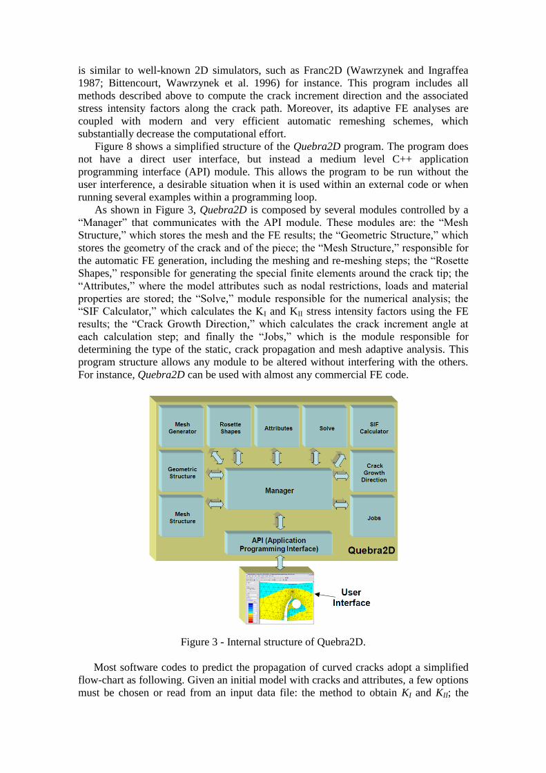
Figure 8 shows a simplified structure of the Quebra2D program. The program does

not have a direct user interface, but instead a medium level C++ application

programming interface (API) module. This allows the program to be run without the

user interference, a desirable situation when it is used within an external code or when

running several examples within a programming loop.

As shown in Figure 3, Quebra2D is composed by several modules controlled by a

“Manager” that communicates with the API module. These modules are: the “Mesh

Structure,” which stores the mesh and the FE results; the “Geometric Structure,” which

stores the geometry of the crack and of the piece; the “Mesh Structure,” responsible for

the automatic FE generation, including the meshing and re-meshing steps; the “Rosette

Shapes,” responsible for generating the special finite elements around the crack tip; the

“Attributes,” where the model attributes such as nodal restrictions, loads and material

properties are stored; the “Solve,” module responsible for the numerical analysis; the

“SIF Calculator,” which calculates the KI and KII stress intensity factors using the FE

results; the “Crack Growth Direction,” which calculates the crack increment angle at

each calculation step; and finally the “Jobs,” which is the module responsible for

determining the type of the static, crack propagation and mesh adaptive analysis. This

program structure allows any module to be altered without interfering with the others.

For instance, Quebra2D can be used with almost any commercial FE code.

Figure 3 - Internal structure of Quebra2D.

Most software codes to predict the propagation of curved cracks adopt a simplified

flow-chart as following. Given an initial model with cracks and attributes, a few options

must be chosen or read from an input data file: the method to obtain KI and KII; the

crack increment direction criterion; the equivalent SIF Keq criterion; the propagation

threshold Kth; the material or structure toughness KC; the load ratio R = Kmin/Kmax; the

material da/dN constants such as Paris’ A and m (when dealing with multiple cracks that

can interact); the maximum crack increment size a; and the number of steps or

increments required to simulate the crack path, called #steps. The next procedure is to

create a mesh in the model domain, as described in the last section, followed by the FE

analysis. Then, the equivalent SIF Ki and the global angle of crack propagation

direction θi are obtained from the FE results, for each crack in the model. In addition,

the maximum equivalent SIF Kmax is obtained searching through all Ki, and the

equivalent SIF at the maximum load is found from the load ratio R by Kmax = Kmax/(1 –

R). After finishing all these tasks, the entire process is restarted for the next growth step.

However, such brute force numerical calculation is not efficient for long variable

amplitude loading histories, causing in the general case different crack increments at

each load cycle. This requires remeshing and time-consuming recalculations in FE for

every load cycle. Moreover, load interaction effects such as crack retardation

compromise even more the computational efficiency of this approach.

However, the local approach can be efficiently used to calculate the crack increment

at each load cycle, considering crack retardation effects if necessary. The local approach

is so called because it does not require the global solution of the structure stress field. It

is based on the direct integration of the fatigue crack propagation rule of the material,

da/dN = F(K, Kmax, Kth, KC, ...), where K and Kmax, the stress intensity range and

maximum, are the two fatigue cracking driving forces; Kth and KC, the fatigue crack

propagation threshold and the toughness of the material-structure set, are the material

related properties which induce the sigmoidal shape of typical da/dN curves; whereas

the ellipsis represent the possible influence of other parameters, such as the opening SIF

Kop, or non-mechanical (environmental or chemical, e.g.) driving forces. Appropriate

stress intensity factor expressions for K and for the da/dN rule must be used to obtain

satisfactory cracking life predictions.

However, the need for the stress intensity expression of the crack is a major

drawback of the local approach, because it is simply not available for most real

components, in which cracks tend to curve while they cross non-uniaxial stress fields.

Therefore, designers must use engineering common sense to choose approximate KI

handbook expressions to solve real problems. The error involved in such

approximations obviously increases as the real crack deviates from the modeled crack,

and in such cases the accuracy of the local approach is questionable and its predictions

unreliable. But this problem can be efficiently solved as follows.

Since the advantages of the global and local approaches are complementary, the

problem can be successfully divided into two steps. First, an appropriate FE program

(such as Quebra2D) is used to calculate the generally curved crack path and its

associated Mode I stress intensity factor KI(a) along the crack length a, under constant

amplitude loading. Then, an analytical expression is adjusted to the discrete KI(a) values

calculated at as many points as required along the crack path, to be used as input to a

local approach program (such as the ViDa program, described below). Finally, the

actual variable amplitude loading can be efficiently treated by the direct integration of

the crack propagation rule, considering retardation effects if required. Neither the K

expression nor the type of crack propagation rule should have their accuracy

compromised when using this approach, a hypothesis experimentally verified in many

cases.

The local approach program used in this work is named ViDa (which means life in

Portuguese). This piece of software has been developed to automate all the traditional

local approach methods used in fatigue design (Meggiolaro and Pinho de Castro 1998;

Castro and Meggiolaro 1999), including the SN, the IIW (for welded structures) and the

N methods for crack initiation, and the da/dN method for crack propagation. The crack

propagation life can be calculated by the Krms or the cycle-by-cycle methods, for either

planar or 3D problems, as long as the stress intensity factor expressions are provided

(which have been calculated by Quebra2D).

Several load interaction models are included in the ViDa software (Willenborg,

Engle et al. 1971; Wheeler 1972; Gallagher 1974; Bunch, Trammell et al. 1996).

Wheeler’s model e.g., perhaps one of the simplest and most well known (Wheeler

1972), introduces a crack-growth reduction factor bounded by zero and unity. This

factor is calculated for each cycle to predict retardation as long as the current plastic

zone Zi is contained within a previously overload-induced plastic zone Zol. The

retardation is maximum just after the overload, and it ends when the border of Zi

touches the border of Zol.

Therefore, if aol and ai are the crack sizes at the instant of the overload and at the

(later) i-th cycle, and (da/dN)ret,i and (da/dN)i are the retarded and the corresponding

non-retarded crack growth rates (at which the crack would be growing in the i-th cycle

if the overload had not occurred), then, according to Wheeler

iolol

i

iiret aaZ

Z

dN

da

dN

da

,

, if ai + Zi < aol + Zol (1)

where is an experimentally adjustable constant, obtained by selecting the closest

match between an experimentally measured curve under variable amplitude loading and

the predicted crack growth curves using several -value candidates. But this model

cannot predict crack arrest because the resulting (da/dN)ret,i is always positive. Cut-off

values have been proposed to include crack arrest in the original Wheeler model,

however this approach results in discontinuous (da/dN)ret,i equations.

Meggiolaro and Castro (Meggiolaro and Castro 2001) used a simple but effective

modification to the original Wheeler model in order to predict both crack retardation

and arrest. This approach, called the Modified Wheeler model, uses a Wheeler-like

parameter to multiply K instead of da/dN after the overload

iolol

iiiret

aaZ

ZaKaK )()( , if ai + Zi < aol + Zol (2)

where Kret(ai) and K(ai) are the values of the stress intensity ranges that would be

acting at ai with and without retardation due to the overload, and is an experimentally

adjustable constant, in general different from the original Wheeler model exponent .

This simple modification can be used with any of the propagation rules that recognize

Kth to predict both retardation and arrest of fatigue cracks after an overload, the arrest

occurring if Kret(ai) Kth.

Another crack retardation model included in ViDa is the Constant Closure model,

originally developed at Northrop for use in their classified programs (Bunch, Trammell

et al. 1996). This load interaction model is based on the observation that for some

variable amplitude load histories the closure stress does not deviate significantly from a

certain stabilized value. This stabilized value is determined by assuming that the

spectrum has a “controlling overload” and a “controlling underload” that occur often

enough to keep the residual stresses constant, and thus the closure level constant.

In the constant closure model, the opening stress intensity factor Kop is the only

empirical parameter, with typical values estimated between 20% and 50% of the

maximum overload stress intensity factor. The value of Kop, calculated for the

controlling overload event, is then applied to the following (smaller) loads to compute

crack growth, recognizing crack retardation and even crack arrest (if Kmax Kop).

The main limitation of the Constant Closure model is that it can only be applied to

loading histories with “frequent controlling overloads,” because it does not model the

decreasing retardation effects as the crack tip cuts through the overload plastic zone. In

this model, it is assumed that a new overload zone, with primary plasticity, is formed

often enough before the crack can significantly propagate through the previous plastic

zone, thus not modeling secondary plasticity effects by keeping Kop constant.

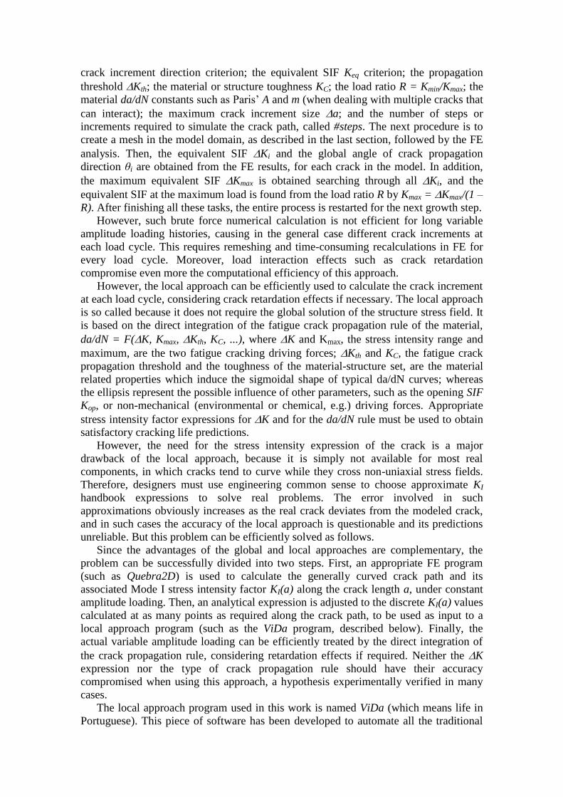
4. COMPARISON AMONG STRESS INTENSITY FACTOR PREDICTIONS

Sinclair (Sinclair 2004) presents an extensive review of SIF numerical predictions.

However, most comparisons are somewhat incomplete in at least one of three important

aspects. First, they discuss numerical results generated by “artificial” meshes that do not

adapt to the (growing) crack path, contrary to the automatically generated meshes

presented in this paper. Second, they do not show convergence analysis of the results

when the elements size is decreased around the crack tip, increasing the number of

elements in the analyzed numerical model. Third, they present only Mode I results.

This section compares SIF values obtained by the three methods using the

Quebra2D methodology: the displacement correlation technique (DCT) (Shih, de

Lorenzi et al. 1976); the potential energy release rate, computed by means of a modified

crack-closure integral technique (MCC) (Rybicki and Kanninen 1977; Raju 1987); and

the J-integral, computed by means of the equivalent domain integral (EDI) together

with a mode decomposition scheme (Bui 1983; Banks-Sills and Sherman 1986;

Nikishkov and Atluri 1987; Dodds and Vargas 1988; Chen and Atluri 1989). All three

limitations of previous comparisons available in the literature are overcome. The model

shown in Figure 4(a) is employed to compare the SIF calculated by using the three

different methods in the FE analysis. This model is a representation of a very large plate

with a small crack, aiming to reproduce the infinite plate solution. The plate has 2000

2000mm with an inclined central crack of length 2a = 2mm. The plate is loaded by a

uniform stress in the vertical direction, see Figure 4(a). This example is studied varying

the crack angle with the horizontal axis from 0o to 80

o at 10

o steps. To analyze the SIF

calculation convergence, the density of the FE mesh is modified varying the number n

of the elements at each of the two crack faces, with n = 4, 8, 16, 32, 64, 128, 256 and

512 elements. In all models, eleven nodes are used at each edge of the plate. Figure 4(b)

shows an example of a mesh generated by Quebra2D for the 80o crack with 4 elements

on each of the two crack faces.

Figure 4 - (a) Model used to compare the SIF calculated by the three different methods

and (b) typical FE mesh.

Four different strategies of mesh generation were considered in the model, featuring

meshes with or without additional refinement to force equal size between neighboring

cells near the crack tip (see Figure 1) and, for either case, with or without performing

additional smoothing on the final meshes. In this way, elements around the crack tip

ended up different in shape and arrangement. FE analyses were performed for each of

the 4 meshing strategies, for 8 different numbers of crack face elements (n = 4, 8, 16,

32, 64, 128, 256 and 512), 9 considered crack angles (00, 10

0, …, 80

0), and 3 KI

calculation models (DCT, MCC and EDI), resulting in 864 calculations. It was found

that the KI calculation errors do not significantly depend on the meshing strategy or

crack angle, but they’re very much influenced by the number of crack face elements and

calculation model. Figures 5 and 6 show the ratio between the FE-calculated and the

actual (theoretical) Mode I or II SIF for different crack angles and calculation methods,

as a function of the number of crack face elements.

Figure 5 - Ratio between the FE-calculated and the actual Mode I SIF for different crack

angles and calculation methods, as a function of the number of crack face elements; the

dashed lines are averages over the nine analyzed crack angles (00, 10

0, …, 80

0).

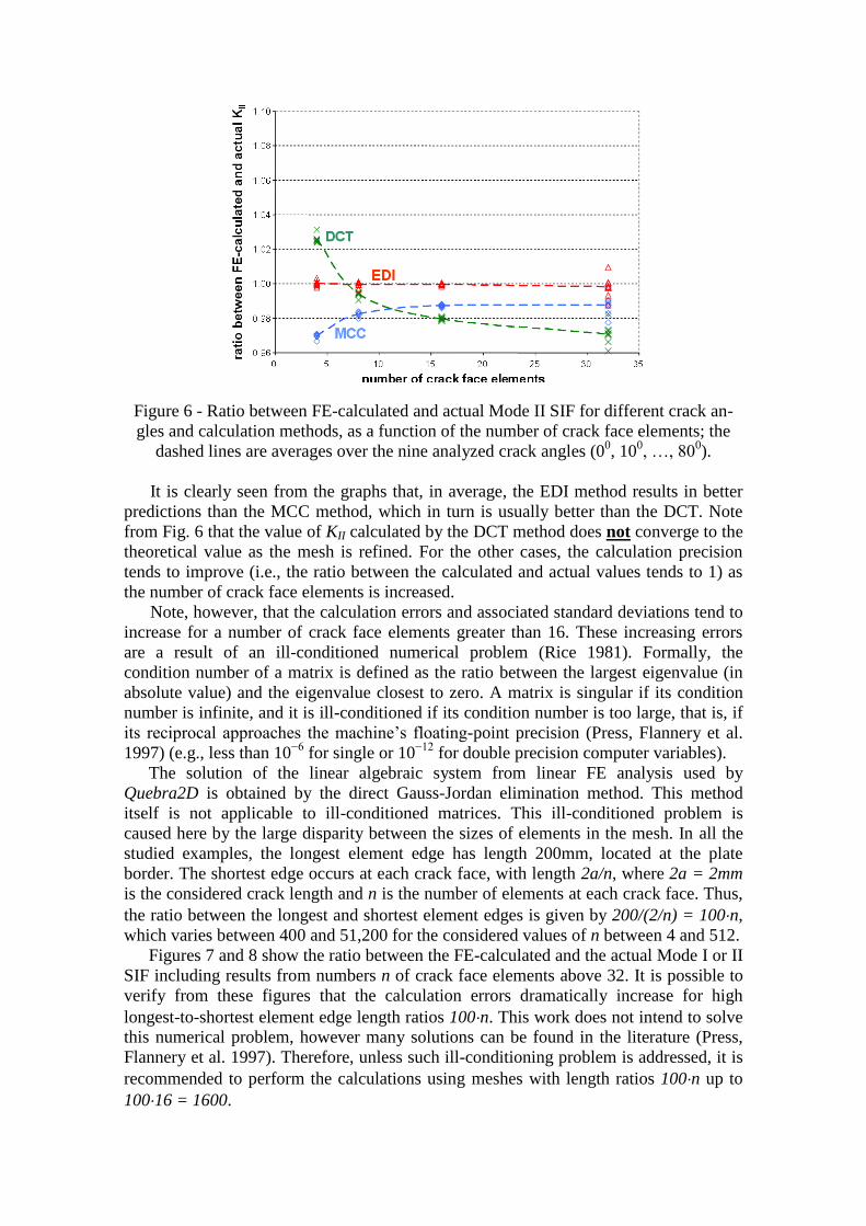
Figure 6 - Ratio between FE-calculated and actual Mode II SIF for different crack an-

gles and calculation methods, as a function of the number of crack face elements; the

dashed lines are averages over the nine analyzed crack angles (00, 10

0, …, 80

0).

It is clearly seen from the graphs that, in average, the EDI method results in better

predictions than the MCC method, which in turn is usually better than the DCT. Note

from Fig. 6 that the value of KII calculated by the DCT method does not converge to the

theoretical value as the mesh is refined. For the other cases, the calculation precision

tends to improve (i.e., the ratio between the calculated and actual values tends to 1) as

the number of crack face elements is increased.

Note, however, that the calculation errors and associated standard deviations tend to

increase for a number of crack face elements greater than 16. These increasing errors

are a result of an ill-conditioned numerical problem (Rice 1981). Formally, the

condition number of a matrix is defined as the ratio between the largest eigenvalue (in

absolute value) and the eigenvalue closest to zero. A matrix is singular if its condition

number is infinite, and it is ill-conditioned if its condition number is too large, that is, if

its reciprocal approaches the machine’s floating-point precision (Press, Flannery et al.

1997) (e.g., less than 10−6

for single or 10−12

for double precision computer variables).

The solution of the linear algebraic system from linear FE analysis used by

Quebra2D is obtained by the direct Gauss-Jordan elimination method. This method

itself is not applicable to ill-conditioned matrices. This ill-conditioned problem is

caused here by the large disparity between the sizes of elements in the mesh. In all the

studied examples, the longest element edge has length 200mm, located at the plate

border. The shortest edge occurs at each crack face, with length 2a/n, where 2a = 2mm

is the considered crack length and n is the number of elements at each crack face. Thus,

the ratio between the longest and shortest element edges is given by 200/(2/n) = 100n,

which varies between 400 and 51,200 for the considered values of n between 4 and 512.

Figures 7 and 8 show the ratio between the FE-calculated and the actual Mode I or II

SIF including results from numbers n of crack face elements above 32. It is possible to

verify from these figures that the calculation errors dramatically increase for high

longest-to-shortest element edge length ratios 100n. This work does not intend to solve

this numerical problem, however many solutions can be found in the literature (Press,

Flannery et al. 1997). Therefore, unless such ill-conditioning problem is addressed, it is

recommended to perform the calculations using meshes with length ratios 100n up to

10016 = 1600.

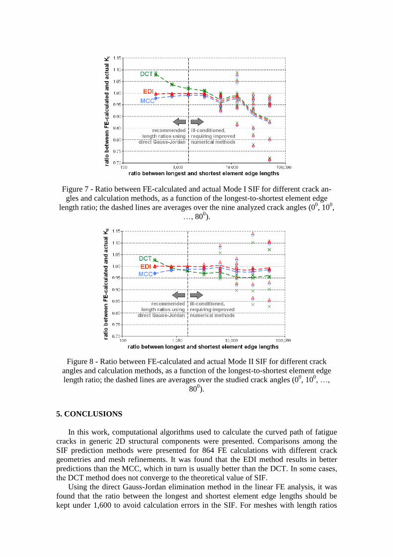
Figure 7 - Ratio between FE-calculated and actual Mode I SIF for different crack an-

gles and calculation methods, as a function of the longest-to-shortest element edge

length ratio; the dashed lines are averages over the nine analyzed crack angles (00, 10

0,

…, 800).

Figure 8 - Ratio between FE-calculated and actual Mode II SIF for different crack

angles and calculation methods, as a function of the longest-to-shortest element edge

length ratio; the dashed lines are averages over the studied crack angles (00, 10

0, …,

800).

5. CONCLUSIONS

In this work, computational algorithms used to calculate the curved path of fatigue

cracks in generic 2D structural components were presented. Comparisons among the

SIF prediction methods were presented for 864 FE calculations with different crack

geometries and mesh refinements. It was found that the EDI method results in better

predictions than the MCC, which in turn is usually better than the DCT. In some cases,

the DCT method does not converge to the theoretical value of SIF.

Using the direct Gauss-Jordan elimination method in the linear FE analysis, it was

found that the ratio between the longest and shortest element edge lengths should be

kept under 1,600 to avoid calculation errors in the SIF. For meshes with length ratios

higher than 1,600, improved numerical methods to deal with ill-conditioned matrices

would be necessary to not compromise the calculation accuracy of the calculated SIF.

6. REFERENCES

Alegre, J. M. and I. I. Cuesta (2010). "Some aspects about the crack growth FEM

simulations under mixed-mode loading." International Journal of Fatigue 32(7):

1090-1095.

Alshoaibi, A., M. Hadi, et al. (2007). "An adaptive finite element procedure for crack

propagation analysis." Journal of Zhejiang University - Science A 8(2): 228-236.

Azócar, D., M. Elgueta, et al. (2010). "Automatic LEFM crack propagation method

based on local Lepp-Delaunay mesh refinement." Advances in Engineering

Software 41(2): 111-119.

Banks-Sills, L. and D. Sherman (1986). "Comparison of Method for Calculating Stress-

Intensity Factors with Quarter-Point Elements." International Journal of Fracture

Mechanics 32: 127-140.

Bittencourt, T. N., P. A. Wawrzynek, et al. (1996). "Quasi-automatic simulation of

crack propagation for 2D LEFM problems." Engineering Fracture Mechanics

55(2): 321-334.

Bouchard, P. O., F. Bay, et al. (2003). "Numerical modelling of crack propagation:

Automatic remeshing and comparison of different criteria." Computer Methods

in Applied Mechanics and Engineering 192(35-36): 3887-3908.

Bouchard, P. O., F. Bay, et al. (2000). "Crack propagation modelling using an advanced

remeshing technique." Computer Methods in Applied Mechanics and

Engineering 189(3): 723-742.

Bui, H. D. (1983). "Associated Path Independent J-Integrals for Separating Mixed

Modes." Journal of Mechanics & Physics Solids 13: 439-448.

Bunch, J. O., R. T. Trammell, et al. (1996). "Structural life analysis methods used on the

B-2 bomber." ASTM Special Technical Publication: 220-247.

Castro, J. T. P. and M. A. Meggiolaro (1999). "Some Comments on the eN Method

Automation for Fatigue Dimensioning under Complex Loading (in Portuguese)."

Revista Brasileira de Ciências Mecânicas 21: 294-312.

Cavalcante Neto, J. B., P. A. Wawrzynek, et al. (2001). "An algorithm for three-

dimensional mesh generation for arbitrary regions with cracks." Engineering

with Computers 17(1): 75-91.

Chan, C. T. and K. Anastasiou (1997). "Automatic tetrahedral mesh generation scheme

by the advancing front method." Communications in Numerical Methods in

Engineering 13(1): 33-46.

Chen, K. L. and N. Atluri (1989). "Comparison of Different Methods of Evaluation of

Weight Functions for 2D Mixed-Mode Fracture Analysis." Engineering Fracture

Mechanics 34: 935-956.

Dodds, R. H. J. and P. M. Vargas (1988). Numerical Evaluation of Domain and Contour

Integrals for Nonlinear Fracture Mechanics. Urbana-Champaign, University of

Illinois.

Erdogan, F. and G. C. Sih (1963). "On the Crack Extension in Plates under Plane

Loading and Transverse Shear." Journal of Basic Engineering 85: 519-527.

Gallagher, R. H. (1974). A Generalized Development of Yield Zone Models, Wright

Patterson Air Force Laboratory.

Heintz, P. (2006). "On the numerical modelling of quasi-static crack growth in linear

elastic fracture mechanics." International Journal for Numerical Methods in

Engineering 65(2): 174-189.

Hussain, M. A., S. U. Pu, et al. (1974). Strain Energy Release Rate for a Crack under

Combined Mode I and II. ASTM STP 560: 2-28.

Ingraffea, A. R. (2004). Computational Fracture Mechanics. Encyclopedia of

Computational Mechanics, John Wiley and Sons.

Ingraffea, A. R. and P. A. Wawrzynek (2003). Finite Element Methods for Linear

Elastic Fracture Mechanics. Comprehensive Structural Integrity. R. d. B. a. H.

Mang. Oxford, England, Elsevier Science Ltd.

Jin, H. and R. I. Tanner (1993). "Generation of unstructured tetrahedral meshes by

advancing front technique." International Journal for Numerical Methods in

Engineering 36(11): 1805-1823.

Khoei, A. R., H. Azadi, et al. (2008). "Modeling of crack propagation via an automatic

adaptive mesh refinement based on modified superconvergent patch recovery

technique." Engineering Fracture Mechanics 75(10): 2921-2945.

Lim, I. L., I. W. Johnston, et al. (1992). "Comparison between various displacement-

based stress intensity factor computation techniques." International Journal of

Fracture 58(3): 193-210.

Lim, I. L., I. W. Johnston, et al. (1996). "A finite element code for fracture propagation

analysis within elasto-plastic continuum." Engineering Fracture Mechanics

53(2): 193-211.

Lo, S. H. (1985). "A New Mesh Generation Sheme for Arbitrary Planar Domains."

International Journal for Numerical Methods in Engineering 21(8): 1403-1426.

Lohner, R. and P. Parikh (1988). "Generation of threedimensional unstructured grids by

the advancing-front method." International Journal for Numerical Methods in

Fluids 8: 1135–1149.

Meggiolaro, M. A. and J. T. P. Castro (2001). An Evaluation of Elber-Type Crack

Retardation Models. II Seminário Internacional de Fadiga (SAE-Brasil). São

Paulo. SAE no. 2001-01-4063: 207-216.

Meggiolaro, M. A. and J. T. Pinho de Castro (1998). "ViDa 98 - visual damagemeter to

automatize the fatigue design under complex loading." Revista Brasileira de

Ciencias Mecanicas/Journal of the Brazilian Society of Mechanical Sciences

20(4): 666-685.

Miranda, A. C., J. B. Cavalcante Neto, et al. (1999). "An algorithm for two-dimensional

mesh generation for arbitrary regions with cracks." XII Brazilian Symposium on

Computer Graphics and Image Processing (Cat. No.PR00481): 29-38.

Miranda, A. C. O., L. F. Martha, et al. (2009). "Surface mesh regeneration considering

curvatures." Engineering with Computers 25(2): 207-219.

Miranda, A. C. O., M. A. Meggiolaro, et al. (2002). Fatigue Crack Propagation under

Complex Loading in Arbitrary 2D Geometries. Applications of Automation

Technology in Fatigue and Fracture Testing and Analysis. M. P. Braun AA,

Lohr RD. ASTM STP 1411: 120-146.

Miranda, A. C. O., M. A. Meggiolaro, et al. (2003). "Fatigue life and crack path

predictions in generic 2D structural components." Engineering Fracture

Mechanics 70(10): 1259-1279.

Miranda, A. C. O., M. A. Meggiolaro, et al. (2003). "Fatigue life prediction of complex

2D components under mixed-mode variable amplitude loading." International

Journal of Fatigue 25(9-11): 1157-1167.

Moller, P. and P. Hansbo (1995). "On advancing front mesh generation in three

dimensions." International Journal for Numerical Methods in Engineering

38(21): 3551-3569.

Nikishkov, G. P. and S. N. Atluri (1987). "Calculation of Fracture Mechanics

Parameters for an Arbitrary Three-Dimensional Crack by the Equivalent

Domain Integral Method." International Journal for Numerical Methods in

Engineering 24(9): 1801-1821.

Paris, P. C., M.P. Gomez, et al. (1961). "A rational analytic theory of fatigue." The

Trend in Engineering 13: 9-14.

Paulino, G. H., I. F. M. Menezes, et al. (1999). "A Methodology for Adaptive Finite

Element Analysis: Towards an Integrated Computational Environment."

Computational Mechanics 23: 361-388.

Peraire, J., J. Peiro, et al. (1988). "Finite Euler computation in three-dimensions."

International Journal for Numerical Methods in Engineering 26: 2135–2159.

Phongthanapanich, S. and P. Dechaumphai (2004). "Adaptive Delaunay triangulation

with object-oriented programming for crack propagation analysis." Finite

Elements in Analysis and Design 40(13-14): 1753-1771.

Press, W. H., B. P. Flannery, et al. (1997). Numerical Recipes in C: The Art of

Scientific Computing. New York, Cambridge University Press.

Quadros, W. R., V. Vyas, et al. (2010). "A computational framework for automating

generation of sizing function in assembly meshing via disconnected skeletons."

Engineering with Computers 26(3): 231-247.

Raju, I. S. (1987). "Calculation of strain-energy release rates with higher order and

singular finite elements." Engineering Fracture Mechanics 28(3): 251-274.

Rassineux, A. (1998). "Generation and optimization of tetrahedral meshes by advancing

front technique." International Journal for Numerical Methods in Engineering

41(4): 651-674.

Rice, J. R. (1981). Matrix computations and mathematical software, McGraw-Hill

Rozumek, D., C. T. Lachowicz, et al. (2010). "Analytical and numerical evaluation of

stress intensity factor along crack paths in the cruciform specimens under out-of-

phase cyclic loading." Engineering Fracture Mechanics 77(11): 1808-1821.

Rybicki, E. F. and M. F. Kanninen (1977). "A finite element calculation of stress

intensity factors by a modified crack closure integral." Engineering Fracture

Mechanics 9(4): 931-938.

Shih, C. F., H. G. de Lorenzi, et al. (1976). "Crack Extension Modeling with Singular

Quadratic Isoparametric Elements." International Journal of Fatigue 12: 647-

651.

Sih, G. C. (1974). "Strain-energy-density factor applied to mixed mode crack

problems." International Journal of Fracture 10(3): 305-321.

Sinclair, G. (2004). "Stress Singularities in Classical Elasticity–I: Removal,

Interpretation, and Analysis." Applied Mechanics Reviews 57(4): 251-298.

Wawrzynek, P. A. and A. R. Ingraffea (1987). "Interactive finite element analysis of

fracture processes: An integrated approach." Theoretical and Applied Fracture

Mechanics 8(2): 137-150.

Wheeler, O. E. (1972). "Spectrum loading and crack growth." Transactions of the

ASME. Series D, Journal of Basic Engineering 94(1): 181-186.

Willenborg, J., R. M. Engle, et al. (1971). Crack Growth Retardation Model Using an

Effective Stress Concept. A. F. F. D. Laboratory, Wreight Patterson Air Force

Base.