BioOne sees sustainable scholarly publishing as an inherently collaborative enterprise connecting authors, nonprofit publishers, academic institutions, researchlibraries, and research funders in the common goal of maximizing access to critical research.

Comparing Two Ground-Cover Measurement Methodologies for SemiaridRangelandsAuthor(s): Keith T. Weber , Fang Chen , D. Terrance Booth , Mansoor Raza , Kindra Serr , and BhushanGokhaleSource: Rangeland Ecology & Management, 66(1):82-87. 2013.Published By: Society for Range ManagementDOI: http://dx.doi.org/10.2111/REM-D-11-00135.1URL: http://www.bioone.org/doi/full/10.2111/REM-D-11-00135.1

BioOne (www.bioone.org) is a nonprofit, online aggregation of core research in the biological, ecological, andenvironmental sciences. BioOne provides a sustainable online platform for over 170 journals and books publishedby nonprofit societies, associations, museums, institutions, and presses.

Your use of this PDF, the BioOne Web site, and all posted and associated content indicates your acceptance ofBioOne’s Terms of Use, available at www.bioone.org/page/terms_of_use.

Usage of BioOne content is strictly limited to personal, educational, and non-commercial use. Commercial inquiriesor rights and permissions requests should be directed to the individual publisher as copyright holder.

Rangeland Ecol Manage 66:82–87 | January 2013 | DOI: 10.2111/REM-D-11-00135.1

Comparing Two Ground-Cover Measurement Methodologies for Semiarid Rangelands

Keith T. Weber,1 Fang Chen,2 D. Terrance Booth,3 Mansoor Raza,4 Kindra Serr,5

and Bhushan Gokhale4

Authors are 1GIS Director, 2Postdoctoral Research Associate, 4Research Assistant, and 5Systems Administrator, GIS Training and Research Center, IdahoState University, Pocatello, ID 83209, USA; and 3Rangeland Scientist, USDA-ARS High Plains Grassland Research Station, Cheyenne, WY 82009, USA.

Abstract

The limited field of view (FOV) associated with single-resolution very-large-scale aerial (VLSA) imagery requires users tobalance FOV and resolution needs. This balance varies by the specific questions being asked of the data. Here, we tested a FOV-resolution question by comparing ground cover measured in the field with the use of point-intercept transects with similar datameasured from 50-mm-per-pixel (mmpp) VLSA imagery of the same locations. Particular care was given to spatial control ofground and aerial sample points from which observations were made, yet percent cover estimates were very different betweenmethods. An error budget was used to calculate error of location and error of quantification. These results indicated locationerror (43.5%) played a substantial role with significant quantification error (21.6%) also present. We conclude that 1) althoughthe georectification accuracy achieved in this project was actually quite good, the level of accuracy required to match groundand aerial sample points represents an unrealistic expectation with currently available positioning technologies, 2) 50-mmppVLSA imagery is not adequate for accurate species identification or cover assessments of plant functional groups, and 3) thebalance between resolution and FOV needs is best addressed by using multiple cameras to acquire nested imagery at multipleVLSA resolutions simultaneously. We recommend ground cover be measured from 1-mmpp imagery and that the imagery benested in lower-resolution, larger FOV images simultaneously acquired.

Key Words: aerial imagery, GIS, remote sensing, VLSA

INTRODUCTION

Ground cover is the vegetation, litter, rocks, and gravel thatcover bare soil and thereby reduce the risk of erosion (Bransonet al. 1972). Quick and accurate assessments of ground coverare useful for assessing soil stability (National ResearchCouncil [NRC] 1994) and are highly important for thesustainable management of millions of hectares of rangelandsworldwide. In the past, the evaluation and monitoring ofexpansive landscapes has relied heavily on judgment andexperience (Stoddart and Smith 1955; NRC 1994). However,conventional field surveys and sampling techniques may benearly impossible or simply impractical to implement acrossvast areas like the US intermountain west. As a result, manypeople on all sides of management issues are calling forincreasingly quantitative and expedient monitoring approaches(Donahue 1999) such as those available through remotesensing. New measures are needed that are cost effective andprovide timely information within acceptable error rates (Floydand Anderson 1987; Brady et al. 1995; Brakenhielm andQuighong 1995; Sivanpillai and Booth 2008).

High-spatial-resolution satellite and aerial remote sensinghave been used to conduct numerous studies across large

landscapes. Blumenthal et al. (2007) used high-resolutionimagery to study and measure infestations of invasive terrestrialweeds. Anderson et al. (1996), Bradley and Mustard (2006),Everitt et al. (1995, 1996), and Lass et al. (2005) suggested thatsatellite and aerial imagery can be used to obtain accurateidentification of invasive weeds. Sivanpillai and Booth (2008)used various remote sensing techniques to determine percentcover of vegetation over the 9 000 ha Hay Press Creek Pasturenear Jeffrey City, Wyoming. Most recently, advancements indigital camera development and lens technologies haveimproved image sharpness to 1 mm per pixel (mmpp) (Boothet al. 2006a), resulting in the ability to differentiate plantfunction groups and many plant species (Booth et al. 2007,2010).

One consideration with very-large-scale aerial (VLSA)imagery is the trade-off between spatial resolution and aerialextent. For example, achieving a spatial resolution of 1 mmppcommonly limits resulting scenes to 433 m (12 m2). Inaddition, accurate georectification (6 0.5 pixel; Weber 2006) ofthe imagery is quite difficult due to current limitations ofpositioning technologies such as the NAVSTAR GPS (6 1 cmunder survey conditions). For these reasons, an alternativesolution was sought that could deliver high-spatial-resolutionimagery (50 mmpp), with relatively large individual scene sizes(0.5 km30.5 km), and accurate georectification.

The objectives of this study were to use VLSA imagery (50-mmpp spatial resolution) 1) to compare individual pointobservations read in the field with observations read fromaerial imagery to understand the current capabilities anduncertainty associated with the use of VLSA imagery better,and 2) to compare percent ground-cover measurements derivedfrom field observations with percent ground-cover measure-ments derived from aerial photography to improve range

This study was made possible by a grant from the National Aeronautics and SpaceAdministration Goddard Space Flight Center (NNX08AO90G). Idaho State University(ISU) acknowledges the Idaho Delegation for their assistance in obtaining this grant.

Presented to the symposium, Very-High Resolution Imaging for Resources Monitoring,9–10 February 2011, Billings, MT, USA.

Correspondence: Keith T. Weber, GIS Training and Research Center, Idaho State

University, 921 South 8th Ave, Stop 8104, Pocatello, ID 83209, USA. Email:

webekeit@isu.edu

Manuscript received 2 August 2011; manuscript accepted 12 July 2012.

ª 2013 The Society for Range Management

82 RANGELAND ECOLOGY & MANAGEMENT 66(1) January 2013

scientists’ understanding of the management implications ofVLSA imagery.

METHODS

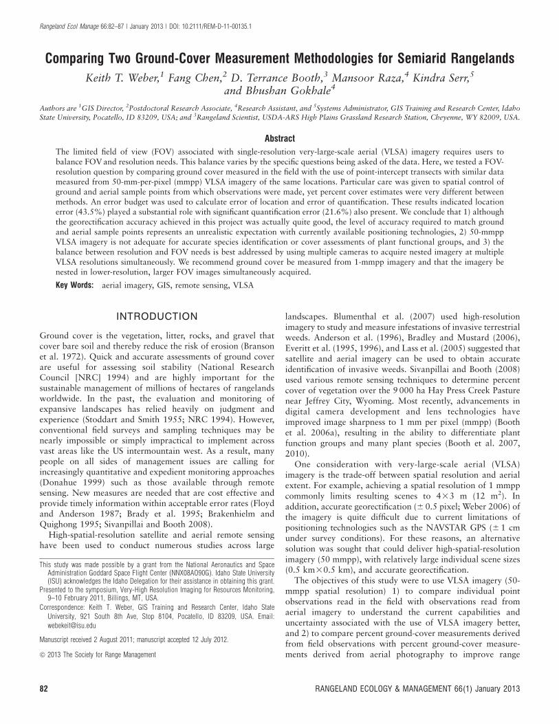
Study AreaThe study was conducted in the sagebrush-steppe rangelands ofsoutheast Idaho, approximately 30 km south of Pocatello,

Idaho, at the O’Neal Ecological Reserve (Fig. 1). This 50-hasite contains sagebrush-steppe upland areas located on lavabenches. The Reserve receives , 380 mm of precipitationannually (primarily in the winter) and is relatively flat, withelevation ranging from 1401 to 1430 m. The dominant plantspecies is big sagebrush (Artemisia tridentata Nutt.), withvarious native and nonnative grasses, including Indian ricegrass (Oryzopsis hymenoides [R. & S.] Ricker.) and needle-

and-thread (Stipa comata Trin. & Rupr.).

Aerial Photography AcquisitionVLSA natural-color digital photography (50-mmpp groundsample distance [GSD] [25-cm2 aerial extent of each pixel]) wasacquired by Valley Air Photo (Boise, Idaho) on 22 May 2009.All images were collected 6 2 h of solar noon (1230 hoursMST) to minimize shadow, and were acquired at a mean height

of 450 m aboveground (mean flight speed¼ 240 km/h groundspeed). Images were collected using a Zeiss RMK Top 15camera with Pleogon A3 wide-angle lens having a calibrated

focal length of 152.812 mm, an angular field of view (FOV) of938 (diagonal), and continuous aperture of f/4 to f/22. Theimagery was then scanned at 12-lm resolution and resampledas a 50-mmpp orthorectified image product. Based upon thesecharacteristics, percent source image distortion was 0% atnadir and up to 10% at the corners of each image. All imageswere delivered in uncompressed TIFF format and georeferencedto Idaho Transverse Mercator (NAD 83).

The georectification accuracy (root means square error[RMSE]) of the imagery as reported in the vendor-suppliedgeospatial metadata was 6 3.17 m (SE¼0.49). The VLSAimagery and location of each transect were corrected to ensureaccurate coregistration with the use of the GPS-acquiredlocation of each start point and the location of each crosspainted on the ground at each start point that was visible in theVLSA imagery.

Field SamplingPercent cover was determined with the use of 30 point-intercepttransects each with 100 observations (Gysel and Lyon 1980;Interagency Technical Team [ITT] 1996). The location oftransect starting points was randomly generated with the use ofHawth’s tools within ArcGIS 9.3.1 and based on the followingcriteria: all points were 1) . 70 m from an edge (road, trail, orfence line) and 2) , 750 m from a road. All transects were readin an east–west direction from the starting point. Prior toacquisition of the aerial imagery, starting points were navigatedto using a Trimble GeoXH GPS receiver (6 0.20 m at 95%confidence interval [CI] after postprocessing). A large cross(mean arm length¼2.0 m and mean arm width¼0.1 m) waspainted on the ground with the use of red spray paint to ensurethe starting point would be readily visible in the imagery (Fig.1). In addition to the physical markers being used to coregisterthe image, the markers served two other purposes: 1) it waseasy for field personnel to revisit each site, and 2) it ensured thesame starting point was used for both field observation andVLSA image interpretation.

During the week of aerial imagery acquisition, fieldpersonnel revisited each sample location and placed a 20-mflexible tape upon the ground from the starting point (indicatedby the painted marker) and in the designated direction (directlyeast or west) with the aid of a compass. To minimize, albeit noteliminate, lens distortion error (Booth et al. 2006b) and yetretain a random sampling design, all transect observations wereread, toward the flight line and hence, toward a point ofdecreasing distortion. Ground-cover type was determined bylooking straight down at the transect tape and recording thecover feature in the uppermost canopy directly indicated at thedesignated observation point. Observation points began at 10cm from the starting point (observation point one) andcontinued every 20 cm thereafter (observation points 2–100).Observation points were measured on the graduated side of thetape measure and had a width of 1 mm. Ground cover at eachobservation point was classified as either shrub, rock (if therock was over 7.5 cm in surface diameter), bare ground,invasive weed, grass, forb, litter, standing dead herbaceousmaterial, standing dead woody material (e.g., a dead tree orsagebrush shrub still intact at the ground), or microbiotic crust.A total of 100 observations were made at each transect and

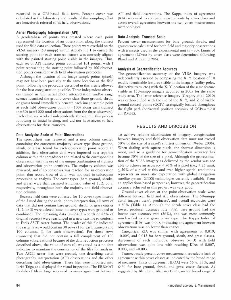
Figure 1. The flight line and 50-mmpp VLSA imagery collected at theO’Neal Ecological Reserve in 2009. Inset shows an example of the imageryand illustrates the red X painted on the ground (circled). The black dotsextending west to east indicate the location where point observations andcorresponding API observations were made.

66(1) January 2013 83

recorded in a GPS-based field form. Percent cover wascalculated in the laboratory and results of this sampling effortare henceforth referred to as field observations.

Aerial Photography Interpretation (API)A geodatabase of points was created where each pointrepresented the location of an observation along the transectused for field data collection. These points were overlaid on theVLSA imagery (50 mmpp) within ArcGIS 9.3.1 to ensure thestarting point for each transect feature was correctly alignedwith the painted starting point visible in the imagery. Thus,each set of API transect points contained 101 points, with 1point representing the starting point followed by 100 observa-tion points consistent with field observation protocols.

Although the location of the image sample points (pixels)may not have been precisely at the same location as the fieldpoint, following the procedure described in this article allowedfor the best coregistration possible. Three independent observ-ers trained in GIS, aerial photo interpretation, and/or rangescience identified the ground-cover class (bare ground, shrub,or grass) found immediately beneath each image sample pointat each field observation point (n¼100) along each transect(n¼30) (n¼9 000 total observations from the three observers).Each observer worked independently throughout this processfollowing an initial briefing, and did not have access to fieldobservations for these transects.

Data Analysis: Scale of Point ObservationsThe spreadsheet was reviewed and a new column createdcontaining the consensus (majority) cover type (bare ground,shrub, or grass) found for each observation point record. Inaddition, field observation data were imported as a separatecolumn within the spreadsheet and related to the correspondingobservation with the use of the unique combination of transectand observation point identifiers. The majority column wasreviewed, and if no consensus was reached for an observationpoint, that record (row of data) was not used in subsequentprocessing or analysis. The cover types (bare ground, shrubs,and grass) were then assigned a numeric value of 1, 2, or 3,respectively, throughout both the majority and field observa-tion columns.

Because field data were collected for 10 cover types insteadof the 3 used during the aerial photo interpretation, all rows ofdata that did not contain bare ground, shrub, or grass entries(1, 2, or 3) were deleted (note: no cover types were grouped orcombined). The remaining data (n¼2 465 records or 82% oforiginal records) were rearranged in a new text file to conformto Esri’s ASCII raster format. The header of this file indicatedthe raster layer would contain 30 rows (1 for each transect) and100 columns (1 for each observation). For those rows(transects) that did not contain a full complement of 100columns (observations) because of the data reduction processesdescribed above, the value of zero (0) was used as a no-dataindicator to maintain the consistency of the files for analysis.Two ASCII raster files were created, one describing aerialphotography interpretation (API) observations and the otherdescribing field observations. These files were imported intoIdrisi Taiga and displayed for visual inspection. The ERRMATmodule of Idrisi Taiga was used to assess agreement between

API and field observations. The Kappa index of agreement(KIA) was used to compare measurements by cover class andassess overall agreement between the two cover measurementmethodologies.

Data Analysis: Transect ScalePercent cover measurements for bare ground, shrubs, andgrasses were calculated for both field and majority observationswith transects used as the experimental unit (n¼30). Limits ofagreement (LOAs) by cover class were determined followingBland and Altman (1986).

Analysis of Georectification AccuracyThe georectification accuracy of the VLSA imagery wasindependently assessed by comparing the X, Y location of 10readily identifiable features visible in the imagery (utility poles,distinctive trees, etc.) with the X, Y location of the same featurevisible in 150-mmpp imagery acquired in 2005 for the samestudy area. The latter reference imagery (Gregory et al. 2010)was orthorectified with the use of the X, Y, and Z of visibleground control points (GCPs) strategically located throughoutthe flight path (horizontal position accuracy of GCPs¼6 2.0cm RMSE).

RESULTS AND DISCUSSION

To achieve reliable classification of imagery, coregistrationbetween imagery and field observation data must not exceed50% of the size of a pixel’s shortest dimension (Weber 2006).When dealing with square pixels, the shortest dimension ismoot, and so a guideline for georectification accuracy hasbecome 50% of the size of a pixel. Although the georectifica-tion of the VLSA imagery as delivered by the vendor was notable to achieve an accuracy �50% of a pixel (i.e., 6 25 mm),� 50% of a pixel at this and even higher spatial resolutionsrepresents an unrealistic expectation with global navigationsatellite system (GNSS) technologies currently available. Froman applications-based perspective, however, the georectificationaccuracy achieved in this project was very good.

Ground-cover classes at the point-observation scale weredifferent between field and API observations. The 50-mmppaerial imagery users’, producers’, and overall accuracies were, 50% (Table 1). Although the shrub cover class had thelowest producer accuracy rate (9%), bare ground had thelowest user accuracy rate (26%), and was most commonlymisclassified as the grass cover type. The Kappa Index ofagreement (KIA) was 0.008, indicating any agreement betweenobservations was no better than chance.

Categorical KIA was similar with agreements of 0.019,�0.005, and 0.015 for bare ground, shrub, and grass classes.Agreement of each individual observer (n¼3) with fieldobservations was quite low with resulting KIAs of 0.007,0.003, and �0.003.

Transect-scale percent cover measurement revealed a lack ofagreement within cover classes as indicated by the broad rangeof measures (limits of agreement [LOA] were 56%, 53%, and64% for bare ground, shrub, and grass cover classes). Assuggested by Bland and Altman (1986), such a broad range of

84 Rangeland Ecology & Management

measures should be considered unacceptable and indicative

that the two measurement methods are not interchangeable. In

this study, the broad LOAs are attributable in large part to

resolution effects, suggesting that 50-mmpp aerial imagery does

not allow the viewer to resolve ground cover to the same degree

as field-based observations. What is most interesting about

these results and perhaps more central to the focus of this

article is the high degree of disagreement between field and API

observations (cf. KIA¼0.008). In all cases, agreements between

these data were very poor and any agreement was attributed

only to chance. This suggests that although the identification of

ground-cover classes common to semiarid sagebrush-steppe

ecosystems (bare ground, shrubs, and grasses) can be made

with the use of aerial imagery, the spatial resolution of 50-

mmpp is not adequate for accurate ground-cover measurements

(cf. Booth and Cox 2009).

Error of location (Pontius 2000; Weber et al. 2008) helps to

explain some of the disagreement further. For example, if the

tape measure used to identify the transect and its subsequent

observation points was not tight, or if the tape was blown by

the wind during observation, or not perfectly aligned in an

east–west direction, or the observer’s eye was not perfectly

positioned at nadir over the observation point, the probability

of agreement between discrete observations would decrease, as

the observation locations would not be the same. In addition,

errors or slight deviations in compass trend could also have

been a source of variation between field and API observations.

In these cases, the error of location would be more pronounced

at the extremes of the transect. In other words, if the rate of

agreement was better at the first observations relative to the last

observations, a measurable error of location would be

demonstrated. To test for this type of error, the rate of

agreement between first observations (field and API) and last

observations (field and API) was determined. The results of this

comparison revealed that 17 of 30 (57%) first observations

made in the field agreed with the first observations made from

VLSA imagery, whereas only 8 of the last observations agreed

(27%). An error budget was estimated following Pontius

(2000) with the use of the VALIDATE module of Idrisi to

calculate error of location and error of quantification. This

result indicates error of location (43.5%) played a substantial

role, compared to quantification error (21.6%), in the

cumulative error budget associated with this study.

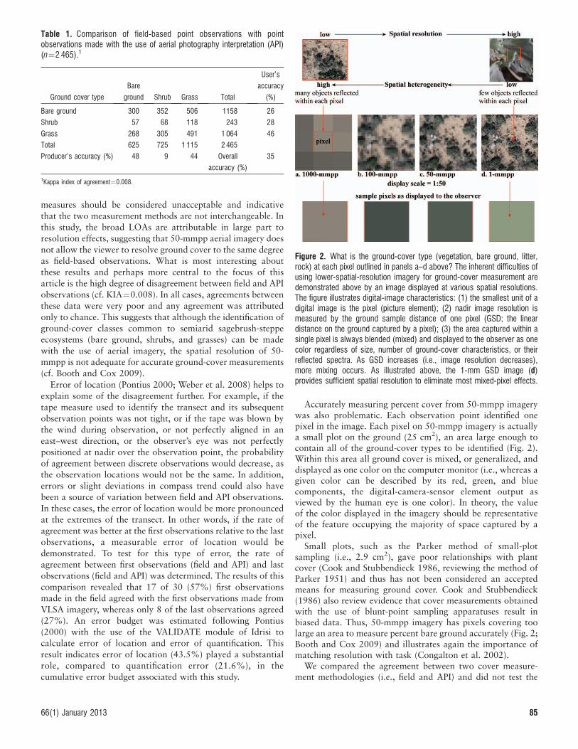
Accurately measuring percent cover from 50-mmpp imagerywas also problematic. Each observation point identified onepixel in the image. Each pixel on 50-mmpp imagery is actuallya small plot on the ground (25 cm2), an area large enough tocontain all of the ground-cover types to be identified (Fig. 2).Within this area all ground cover is mixed, or generalized, anddisplayed as one color on the computer monitor (i.e., whereas agiven color can be described by its red, green, and bluecomponents, the digital-camera-sensor element output asviewed by the human eye is one color). In theory, the valueof the color displayed in the imagery should be representativeof the feature occupying the majority of space captured by apixel.

Small plots, such as the Parker method of small-plotsampling (i.e., 2.9 cm2), gave poor relationships with plantcover (Cook and Stubbendieck 1986, reviewing the method ofParker 1951) and thus has not been considered an acceptedmeans for measuring ground cover. Cook and Stubbendieck(1986) also review evidence that cover measurements obtainedwith the use of blunt-point sampling apparatuses result inbiased data. Thus, 50-mmpp imagery has pixels covering toolarge an area to measure percent bare ground accurately (Fig. 2;Booth and Cox 2009) and illustrates again the importance ofmatching resolution with task (Congalton et al. 2002).

We compared the agreement between two cover measure-ment methodologies (i.e., field and API) and did not test the

Table 1. Comparison of field-based point observations with pointobservations made with the use of aerial photography interpretation (API)(n¼2 465).1

Ground cover type

Bare

ground Shrub Grass Total

User’s

accuracy

(%)

Bare ground 300 352 506 1158 26

Shrub 57 68 118 243 28

Grass 268 305 491 1 064 46

Total 625 725 1 115 2 465

Producer’s accuracy (%) 48 9 44 Overall

accuracy (%)

35

1Kappa index of agreement¼0.008.

Figure 2. What is the ground-cover type (vegetation, bare ground, litter,rock) at each pixel outlined in panels a–d above? The inherent difficulties ofusing lower-spatial-resolution imagery for ground-cover measurement aredemonstrated above by an image displayed at various spatial resolutions.The figure illustrates digital-image characteristics: (1) the smallest unit of adigital image is the pixel (picture element); (2) nadir image resolution ismeasured by the ground sample distance of one pixel (GSD; the lineardistance on the ground captured by a pixel); (3) the area captured within asingle pixel is always blended (mixed) and displayed to the observer as onecolor regardless of size, number of ground-cover characteristics, or theirreflected spectra. As GSD increases (i.e., image resolution decreases),more mixing occurs. As illustrated above, the 1-mm GSD image (d)provides sufficient spatial resolution to eliminate most mixed-pixel effects.

66(1) January 2013 85

accuracy of either method, as this requires a true answer beknown. Although one may argue or assume that fieldobservations represent the truth, this argument is only correctif the observations were repeatable (i.e., have high precision)and without other bias (e.g., observer bias). Furthermore, a trueaccuracy test would require API observations be made at theidentical point observed in the field. Although all attempts weremade to eliminate discrepancies between actual observationpoints, the inherent uncertainty suggests results are best viewedin terms of agreement between methodologies and not a test ofaccuracy.

Comparing various methods used to characterize groundcover in semiarid rangelands is difficult. It is important,however, as range science increasingly embraces geospatialtechnologies. Comparisons demonstrating cross-validationbetween methodologies are critical to bridge the transitionbetween management and monitoring practices that were onceentirely dependent upon field observations to one moredependent upon remotely sensed VLSA imagery. This, however,is also difficult, as performing a reliable cross-validation isdependent upon adequate coregistration, which in turn iscurrently limited by the precision of GNSS positioningtechnologies available in the field (i.e., 6 1 m). To ourknowledge, this is the first article to measure errors of location(43.5%) and quantification (21.6%) in a cumulative errorbudget to build an improved understanding of the complexrelationship between rangeland field and aerial survey meth-odologies. Our results provide important insights for furtherprogress in using ground and aerial data together.

Although both field-based and API observations have theirplace, API observations with VLSA imagery are becoming morecommon and more reliable. VLSA image interpretationpresents several advantages: 1) cover can be measuredanywhere within the imagery regardless of difficulty of accessor proximity to roads, 2) measurements are repeatable (thoughobserver bias is still present [Booth et al. 2006a; Cagney et al.2011]), and 3) the acquired aerial imagery represents anhistorical record of the rangelands that may be used fornumerous other management applications in addition to covermeasurement.

This study tested agreement between ground-cover measure-ments from point-intercept transects and 50-mmpp VLSAimagery. Both individual observation-point and transect-scalepercent cover measurements were compared, with resultsindicating very poor agreement between methodologies. Thisdoes not necessarily indicate that either method was incorrect,however, as the role of locational error cannot be overlookedespecially in heterogeneous environments where ground-coverclasses readily change across even short distances (e.g., 25 mm).Although it may be possible to improve agreement betweenobservations as well as percent cover measurements with theuse of a revised study design and collection of higher spatialresolution imagery (, 50-mmpp), it is more important toappreciate that 1) based upon other studies where higher-spatial-resolution imagery was used, VLSA imagery can be usedto measure ground cover in semiarid rangelands, 2) like allother cover-measurement or estimation methodologies, the useof VLSA imagery and API has limitations (e.g., species cannotbe identified at the spatial resolution used in this study) as wellas advantages, and 3) it is critical to match resolution with task

appropriately. Finally, we conclude that this study’s measures oferror of location (43.5%) and quantification error (21.6%)between rangeland ground and aerial survey methodologiesdefines the current limitations of using ground and aerial datatogether.

MANAGEMENT IMPLICATIONS

The proper design of any API-based ground-cover assessment iscritical to its success and a primary consideration relates to thegranularity of observations. For instance, complete speciesdifferentiation by only aerial imagery, even with a 1-mmppspatial resolution, is not always possible. The 50-mmppimagery used in this study does not provide sufficient clarityto resolve or differentiate shrubs, grasses, and bare ground, andcover assessments of plant functional groups requires a spatialresolution , 50-mmpp (Fig. 2; Booth and Cox 2009; Booth etal. 2010). Although 1-mmpp imagery may be more difficult tocoregister, there are techniques to accomplish reliable coregis-tration, such as the nested imagery technique described byMoffet (2009) and Moffet et al. (2011). This will aid inreducing error of location (a large part of the total errorbudget) and could be applied to either 1-mmpp or 50-mmppimagery in a similar way. However, error of quantification canonly be improved with the use of finer-resolution imagery (e.g.,1 mmpp). Additional research is required to define spatial-resolution guidelines better.

A trade-off between spatial resolution and aerial extentexists and is being addressed with the use of multiple camerasto acquire nested imagery at two or three resolutions (e.g., 1,10, and 20 mmpp [Booth and Cox 2009; Booth et al. 2010])simultaneously. The utility of this approach is evident by thelimited increase in operational costs to obtain multiresolutiondata compared to single-resolution data acquisition (the addedcost is largely the cost of examining the additional images) andin the efficiency demonstrated by Booth et al. (2010), where thelarger FOV was most valuable for assessing an area infestedwith a noxious weed, and where identification of the weed wasconfirmed with the use of nested 1-mmpp imagery.

ACKNOWLEDGMENTS

The authors acknowledge Jamey Anderson, Kerynn Davis, and Heather

Studley (ISU GIS Training and Research Center) for their assistance with

data collection, Kevin Graville (Valley Air Photo) for sharing his expertise

in aerial photogrammetry, and John Welhan and Sue Schou (ISU) for their

assistance with some of the statistical analysis presented in this article.

LITERATURE CITED

ANDERSON, G. L., J. H. EVERITT, D. E. ESCOBAR, N. R. SPENCER, AND R. J. ANDRASCIK. 1996.Mapping leafy spurge (Euphorbia esula) infestations using aerial photographyand geographic information systems. Geocarto International 11:81–89.

BLAND, J. M., AND D. G. ALTMAN. 1986. Statistical methods for assessing agreementbetween two methods of clinical measurement. The Lancet 327:307–310.

BLUMENTHAL, D., D. T. BOOTH, S. E. COX, AND C. E. FERRIER. 2007. Large-scale aerialimages capture details of invasive plant populations. Rangeland Ecology &

Management 60:523–528.

86 Rangeland Ecology & Management

BOOTH, D. T., AND S. E. COX. 2009. Dual-camera, high-resolution aerial assessment ofpipeline revegetation. Environmental Monitoring and Assessment 158:23–33.

BOOTH, D. T., S. E. COX, AND R. D. BERRYMAN. 2006b. Precision measurements from verylarge scale aerial digital imagery. Environmental Monitoring and Assessment

112:293–307.

BOOTH, D. T., S. E. COX, T. W. MEIKLE, AND C. FITZGERALD. 2006a. The accuracy ofground-cover measurements. Rangeland Ecology & Management 59:179–188.

BOOTH, D. T., S. E. COX, AND G. SIMONDS. 2007. Riparian monitoring using 2-cm GSDaerial photography. Ecological Indicators 7:636–648.

BOOTH, D. T., S. E. COX, AND D. TEEL. 2010. Aerial assessment of leafy spurge(Euphorbia esula L.) on Idaho’s deep fire burn. Native Plant Journal 11:327–339.

BRADLEY, B. A., AND J. F. MUSTARD. 2006. Characterizing the landscape dynamics of aninvasive plant and risk of invasion using remote sensing. Ecological Applications

16:1132–1147.BRADY, W. W., J. E. MITCHELL, C. D. BONHAM, AND J. W. COOK. 1995. Assessing the

power of the point-line transect to monitor changes in plant basal cover. Journal

of Range Management 48:187–190.

BRAKENHIELM, S., AND L. QUIGHONG. 1995. Comparison of field methods in vegetationmonitoring. Water Air and Soil Pollution 79:75–87.

BRANSON, F. A., G. F. GIFFORD, AND J. R. OWEN. 1972. Rangeland hydrology: rangescience series no. 1. Denver, CO, USA: Society for Range Management. 84 p.

CAGNEY, J., S. E. COX, AND D. T. BOOTH. 2011. Comparison of point intercept and imageanalysis for monitoring rangeland transects. Rangelands Ecology & Management

64:309–315.

CONGALTON, R. G., K. BIRCH, R. JONES, AND J. SCHRIEVER. 2002. Evaluating remotelysensed techniques for mapping riparian vegetation. Computers and Electronics in

Agriculture 37:113–126.COOK, C. W., AND J. STUBBENDIECK J. 1986. Range research: basic problems and

techniques. Denver, CO, USA: Society for Range Management. 317 p.DONAHUE, D. L. 1999. The western range revisited: removing livestock from public

lands to conserve native biodiversity. Norman, OK, USA: University of OklahomaPress. 352 p.

EVERITT, J. H., G. L. ANDERSON, D. E. ESCOBAR, M. R. DAVIS, N. R. SPENCER, AND R. J.ANDRASCIK. 1995. Use of remote sensing for detecting and mapping leafy spurge(Euphorbia esula). Weed Technology 9:599–609.

EVERITT, J. H., D. E. ESCOBAR, M. A. ALANIZ, M. R. DAVIS, AND J. V. RICHERSON. 1996. Usingspatial information technologies to map Chinese tamarisk (Tamarisk chinensis)infestations. Weed Science 44:194–201.

FLOYD, D. A., AND J. E. ANDERSON. 1987. A comparison of three methods for estimatingplant cover. Journal of Ecology 75:221–228.

GREGORY, J., S. PANDA, AND K. T. WEBER. 2010. Accurate mapping of ground control pointsfor image rectification and holistic planned grazing preparation. In: K. T. Weber andK. Davis [EDS.]. Final report: forecasting rangeland condition with GIS in southeasternIdaho (NNG06GD82G). Pocatello, ID, USA: Idaho State University. p. 49–54.

GYSEL, L. W., AND L. J. LYON. 1980. Habitat analysis and evaluation. In S. D. Schemnitz[ED.]. Wildlife management techniques manual. 4th ed., revised. Washington, DC,USA: The Wildlife Society. p. 305–317.

[ITT] INTERAGENCY TECHNICAL TEAM. 1996. Sampling vegetation attributes. Denver, CO,USA: US Dept of the Interior–Bureau of Land Management National AppliedResources Science Center. Interagency Technical Reference Report BLM/RS/ST-96/002. 164 p.

LASS, L. W., T. S. PRATHER, N. F. GLENN, K. T. WEBER, J. T. MUNDT, AND J. PETTINGILL. 2005.A review of remote sensing of invasive weeds and example of the early detectionof spotted knapweed (Centaurea maculosa) and baby’s-breath (Gypsophila

paniculata) with a hyperspectral sensor. Weed Science 53:242–251.MOFFET, C. A. 2009. Agreement between measurements of shrub cover using ground-

based methods and very large scale aerial imagery. Rangeland Ecology &

Management 62:268–277.MOFFET, C. A., J. B. TAYLOR, AND D. T. BOOTH. 2011. Postfire shrub-cover dynamics: a

70-year fire history in mountain big sagebrush communities. IX InternationalRangeland Congress Proceeding; 2–8 April 2001; Rosario, Argentina.

NORTON, J. 2008. Comparison of field methods. In K. T. Weber [ED.]. Final report:impact of temporal land cover changes in southeastern Idaho rangelands(NNG05GB05G). Pocatello, ID, USA: Idaho State University. p. 41–50.

[NRC] NATIONAL RESEARCH COUNCIL. 1994. Rangeland health. Washington, DC, USA:National Academy Press. 180 p.

PARKER, K. W. 1951. A method for measuring trend in range condition on NationalForest ranges. Washington, DC, USA: USDA Forest Service. 26 p.

PONTIUS, R. G. 2000. Quantification error versus location error in comparison ofcategorical maps. Photogrammetric Engineering and Remote Sensing 66:1011–1016.

SIVANPILLAI, R. D., AND D. T. BOOTH. 2008. Characterizing rangeland vegetation usingLandsat and 1-mm VLSA Data in central Wyoming (USA). Agroforest System

73:55–64.STODDART, L. A., AND A. D. SMITH. 1955. Range management. New York, NY, USA:

McGraw-Hill. 433 pp.WEBER, K. T. 2006. Challenges of integrating geospatial technologies into rangeland

research and management. Rangeland Ecology & Management 59:38–43.WEBER, K. T., J. THEAU, AND K. SERR. 2008. Effect of coregistration error on patchy

target detection using high-resolution imagery. Remote Sensing of Environment

112:845–850.

66(1) January 2013 87