Expert Systems with Applications 39 (2012) 2397–2407

Contents lists available at SciVerse ScienceDirect

Expert Systems with Applications

journal homepage: www.elsevier .com/locate /eswa

Comparing the performance of neural networks developed by usingLevenberg–Marquardt and Quasi-Newton with the gradient descent algorithmfor modelling a multiple response grinding process

Indrajit Mukherjee a,⇑, Srikanta Routroy b

a Shailesh J. Mehta School of Management, Indian Institute of Technology Bombay, Mumbai 400 076, Indiab Mechanical Engineering Department, Birla Institute of Technology & Science, Pilani, Rajasthan, Pilani 333 031, India

a r t i c l e i n f o a b s t r a c t

Keywords:Back propagation neural networkGradient descent algorithmLevenberg–Marquardt algorithmMultiple responseQuasi-Newton algorithm

0957-4174/$ - see front matter � 2011 Elsevier Ltd. Adoi:10.1016/j.eswa.2011.08.087

⇑ Corresponding author. Tel.: +91 22 25767742; faxE-mail addresses: indrajitmukherjee@iitb.ac.in (

troy@gmail.com (S. Routroy).

Monitoring and control of multiple process quality characteristics (responses) in grinding plays a criticalrole in precision parts manufacturing industries. Precise and accurate mathematical modelling of multi-ple response process behaviour holds the key for a better quality product with minimum variability in theprocess. Artificial neural network (ANN)-based nonlinear grinding process model using backpropagationweight adjustment algorithm (BPNN) is used extensively by researchers and practitioners. However, suit-ability and systematic approach to implement Levenberg–Marquardt (L–M) and Boyden, Fletcher, Gold-farb and Shanno (BFGS) update Quasi-Newton (Q-N) algorithm for modelling and control of grindingprocess is seldom explored. This paper provides L–M and BFGS algorithm-based BPNN models for grind-ing process, and verified their effectiveness by using a real life industrial situation. Based on the real lifedata, the performance of L–M and BFGS update Q-N are compared with an adaptive learning (A-L) andgradient descent algorithm-based BPNN model. The results clearly indicate that L–M and BFGS-basednetworks converge faster and can predict the nonlinear behaviour of multiple response grinding processwith same level of accuracy as A-L based network.

� 2011 Elsevier Ltd. All rights reserved.

1. Introduction

In recent years, control of grinding processes by appropriatemathematical models is a key issue in metal cutting industry (Chen& Kumara, 1998; Govindhasamy, MacLoone, Irwin, French, & Doyle,2005; Krajnik, Kopac, & Sluga, 2005; Luong & Spedding, 2002;Mukherjee & Ray, 2006; Petri, Billo, & Bidanda, 1998; Shin &Vishnupad, 1996). However, development of appropriate mathe-matical model is considered to be a formidable and challengingtask in almost all grinding situations (Feng, Wang, & Yu, 2002;Maksoud & Atia, 2004; Sathyanarayanan, Lin, & Chen, 1992; Shaji& Radhakrisnan, 2003). A significant improvement in process effi-ciency may be obtained by these model(s) that identifies anddetermines the critical process variables leading to desired out-put(s) or response(s). To implement appropriate online grindingprocess control mechanism, explicit functional model(s) needs tobe developed by using mechanistic or data-driven empirical mod-elling approach (Box & Draper, 1987; Rowe, Yan, lnasaki, & Malkin,1994). In this context, mechanistic modelling approaches, as pro-posed in literatures (Choi, Subrahmanya, Li, & Shin, 2008; Farago,

ll rights reserved.

: +91 22 25722872.I. Mukherjee), srikantarou-

1976; King & Hahn, 1986; Malkin, 1984, 2007; Moulik, Yang, &Chandrasekhar, 2001), cannot consider all intrinsic process com-plexity manifested due to the presence of a large number of inter-acting variables (Markos, Viharos, & Monostori, 1998). In addition,due to interdependence between various process variables, thesemodels are found to be inaccurate in many situations (Maksoud& Atia, 2004; Petri et al., 1998; Shin & Vishnupad, 1996). Complex-ity of the problem is further enhanced if there are nonlinear multi-ple responses to be modelled simultaneously. There is no adequateand acceptable mechanistic model(s) that can explain varied mul-tiple response grinding situations. Fortunate, empirical models canhandle such nonlinear behaviours, considering the internal com-plexities and dynamics of processes.

Statistical regression (Montgomery & Peck, 1992; Rencher,1995, 1998), fuzzy set theory (Zadeh, 1965) and artificial neuralnetwork (ANN) (Fu, 2003) are some of the empirical modellingtechniques used for prediction and control of grinding processes.These empirical models can be developed based on (i) designedexperimentation data (Kwak, 2005; Montgomery, 2001) or (ii) ac-tual production data, or (iii) by using mixture of production andexperimental data. Using both production and experimental datacan provide a robust mathematical model (Coit, Jackson, & Smith,1998). However, due to many constraints in actual multi-stagemanufacturing environment (Petri et al., 1998; Mukherjee, 2007),

1y

2y

1-st Hidden Layer

Output Layer Input Layer

1v

2v

3v

4v

5v

1 1w

∑

Sigmoidal activation function

Input signal and adjustable weight summation

Output from the neuron

Signal propagation in single neuron

Fig. 1. A multilayered perceptron networks and signal propagation.

2398 I. Mukherjee, S. Routroy / Expert Systems with Applications 39 (2012) 2397–2407

gathering experimental data is too difficult, if not impossible. Someof limitations of designed experimentation-based data collection insuch environment are worth mentioning:

(i) Data are gathered based on additional cost of experimenta-tions, which may be uneconomical in many line-layout typeof mass manufacturing situations (Coit et al., 1998;Mukherjee, 2007).

(ii) Data may not reflect the effect of actual manufacturing envi-ronment (Coit et al., 1998).

(iii) They may be biased to certain operators, or certainprocedures.

Therefore, using actual production data over a period of time invaried process conditions is a viable alternative for many research-ers and practitioners.

Several applications of artificial neural network techniques innonlinear cutting process problems have been reported in the openliteratures. Supervised learning network using back propagationalgorithm, proposed by Rumelhart, Hilton, and Williams (1986),have been successfully applied for modelling (a) a typical creep feedsuper alloy-grinding (Sathyanarayanan et al., 1992), and (b) predic-tion of material removal rate and surface finish parameter of a typ-ical abrasive flow machining (Jain, Jain, & Kalra, 1999). Shin andVishnupad (1996) provide an intelligent grinding process controlscheme based on neuro-fuzzy optimization approach. Chen andKumara (1998) use a hybrid approach of fuzzy set (Zadeh, 1965)and ANN-based technique (ANN) for modelling a grinding process.Petri et al. (1998) develop and propose a backpropagation ANNnetwork (BPNN) model for predicting surface finish, anddimensional accuracy in a grinding process. Cus, Zuperl, andMilfelner (2006) shows the effectiveness and superiority of a modi-fied BPNN as compared to analytical model for cutting force predic-tion of end milling operation. Mukherjee and Ray (2008a) provided asystematic solution methodology for multivariate (linear and non-linear) model development, and implementation for grinding pro-cesses. Kumar and Choudhury (2007) uses a hybrid algorithm,having its root in Levenberg–Marquardt (L–M) algorithm to predictwheel wear and surface roughness of HSS in electro-discharge dia-mond grinding process. Haber and Alique (2003) proposed an intel-ligent supervisory system for tool-wear prediction of millingprocess, created on an ANN network, trained by using L–M algo-rithm. Sorensen, Norgaard, Ravn, and Poulsen (1999) describes acontrol method for non-linear, open-loop unstable, non-mini-mum-phase plants systems based on generalized predictive controlusing Quasi-Newton algorithm-based ANN model. Vafaeesefat(2009) uses a BPNN network trained by L–M to model a creep feedgrinding force and determine its optimal process conditions.

Literature review by the authors on modelling of nonlinearmultiple response grinding processes clearly revealed that thereis only very few research works (Sedighi & Afshari, 2010; Tawakoli,Rabiey, & Lewis, 2009; Urbaniak, 2004) on successful implementa-tion of Levenberg–Marquardt algorithm-based BPNN. However, noapplication of Quasi-Newton (Q-N) algorithm based BPNN ingrinding process modelling is reported in literature. Therefore, aneed is felt to verify the suitability of L–M and Q-N performanceas compared to gradient descent algorithm used in BPNN-basedgrinding process models.

Inspired by this need, this paper first provides a basic theoreti-cal background to develop BPNN networks using gradient descent,Levenberg–Marquardt (L–M), and BFGS update Quasi-Newton(Q-N) algorithm for modelling nonlinear multiple responseprocess. Subsequently, the performances of the trained networksare compared using real life grinding process data. The processdata was collected from an automobile engine manufacturing unit,located in eastern India.

2. Development of backpropagation neural networks

Backpropagation neural network (BPNN) (Rumelhart et al.,1986; Widrow & Lehr, 1990) is a key development and popularchoice for researchers in various process modelling applications(Chen, Lin, Yang, & Tsai, 2010; Coit et al., 1998; Feng et al.,2002; Mukherjee & Ray, 2008b; Sathyanarayanan et al., 1992;Wasserman, 1993; Zhang & Huang, 1995). The prediction abilityof dynamic nonlinear behaviour of multiple responses makesBPNN an attractive choice for many researchers. In addition,the network can be trained without prior assumptions on thefunctional form (e.g. linear, quadratic, higher order polynomialand exponential) or any other distribution assumptions. Theseinherent properties, provide BPNN a clear edge over complexnonlinear regression technique (Basheer & Hajmeer, 2000).

Few of the attractive features of BPNN are:

(i) learning and adoptability allows the process to update ormodify its internal structure according to changingenvironment,

(ii) ability to handle imprecision and fuzzy information andcapability of generalization,

(iii) noise-insensitivity provides accurate prediction in the pres-ence of uncertain data and measuremental error (Bates &Watts, 1988).

In case of fully interconnected artificial neural network withsingle hidden layer neuron processing units (Fig. 1), each neuronhas an adjustable weight factor (wij). wij is the weights assignedfor the connection between node i and j.

The network architecture also has bias terms, which can im-prove convergence property of the network. The nature of mappingrelationship between input and output vectors is defined by theseweights within the network. The input layer acts as an input dataholder that distributes the input to the first hidden layer. The out-puts from the first hidden layer then become the inputs to the sec-ond layer and so on. The last layer acts as the network output layer.In feedback network, signals propagate from output of any neuronto the input of any neuron (Zhang & Huang, 1995). Based on the

I. Mukherjee, S. Routroy / Expert Systems with Applications 39 (2012) 2397–2407 2399

amount of guidance that the learning process receives from outsideagent, network can be further classified as supervised or unsuper-vised. The difference between predicted and target response pro-duces an error signal, which is used to modify the networkweights. The adjustment of weights is intended to be in a directionthat reduces the difference between network output and actual re-sponse vectors. Training set vectors are applied to the networkrepeatedly, until the error measure is at an acceptable value orother convergence criteria of intrinsic algorithm is met. The changein weights may be done at the time each input vector is applied.This is also known as ‘sequential mode of training’. The changecan also be averaged and weights are changed after all the inputvectors are applied. This type of training is called ‘batch mode oftraining’. As this technique work on calculating error starting fromoutput layer down through hidden layer, it is named as ‘back prop-agation of error’ with modified delta rule (Bates & Watts, 1988;Rumelhart et al., 1986).

The performance measure generally used to compare differentlearning algorithm is mean-square of error or MSE (Mukherjee,2007; Tsai & Wang, 2001), and expressed as

MSEðtÞ ¼ 1Np

XN

i¼1

Xk¼p

k¼1

dik

� �2� yi

k

� �2� �

; ð1Þ

where t is the number of training epoch completed. yik is the kth

network predicted output activation of ith training pattern, dik is

the kth actual or observed output of the of ith training pattern,and N is the total number of training pattern.

Backpropagation calculate the derivative of the performancefunction with respect to weight and bias variable matrix (W). Eachvariable in W is adjusted according to the gradient descent algo-rithm (Rardin, 2003) with momentum and learning rate.

dWt ¼ mcdWt�1 þ lrmcdðPerformance FunctionÞ

dWt; ð2Þ

where t is the number of epoch. Wt�1 is the previous change to theweight or bias, lr is the learning rate, mc is the momentum coeffi-cient, and performance objective function is assumed to be of qua-dratic form. A brief discussion on momentum coefficient, learningrate, and number of epoch is given below.

Momentum coefficientMomentum coefficient (Hagan, Demuth, & Beale, 2002; Howard

& Beale, 1998) describes the proportion of the weight change thatis added to each subsequent weight change. Low momentumcauses weight oscillation and instability, and preventing the net-work from learning. High momentum can cripple network adapt-ability. For stable back-propagation, the momentum factorshould be kept less than one. Momentum factors close to unity isneeded to smooth error oscillations. During the middle of training,when steep slope occurs, a small momentum factor is recom-mended. However, during the end of training, large momentumfactor is desirable.

Learning rateError surface for multilayer perceptron may vary in different re-

gions of parameter space. Using simple steepest descent BPNN ap-proach, learning rate (Hagan et al., 2002) is usually kept at aconstant throughout the training phase. However, if the learningrate is too high, the algorithm may oscillate and become unstable.In contrary, if the learning rate is too small, the algorithm will taketoo long to converge (Howard & Beale, 1998). Variable learningrate provides better flexibility to handle such situations.

Number of epochsOn a particular epoch, each training cases are submitted to the

network. Then the target and actual outputs are compared to seethe error performance. The error measure together with the errorsurface gradient is used to adjust the weights. This process is

repeats. The initial network weight configuration is selected at ran-dom. The learning of the network stops, as soon as any of the fol-lowing conditions is satisfied:

(i) maximum number of epoch (repetitions) predefined isreached,

(ii) maximum amount of iteration time given has been reached,(iii) minimum level of error performance is reached,(iv) performance gradient falls below the minimum gradient

predefined.

In this paper, for all the three algorithms selected, the conver-gence criteria or performance goal is set to 0.001 or if number ofepoch reaches 2000. Momentum coefficients, mf is selected as 0.9(Hagan et al., 2002; Howard & Beale, 1998). The choice of squash-ing functions or transfer function (Howard & Beale, 1998) does notseem to be critical as long as the function is non-linear and neuronoutputs are bounded (Wasserman, 1993). However, hyperbolictangent function is selected for this study. It is to be mentionedthat as back propagation algorithm is a steepest decent type ofsearch, there is always a chance for the algorithm to get trappedin local error minima. In addition, selection of intrinsic parametervalues and order of differential functions usually influences theBPNN performance. As and when the learning is completed, the fi-nal values of weights are fixed. The final weights (WFinal) are usedfor testing and other network functional ‘recalling’ sessions. Theregression equation can be expressed as,

bY ¼WFinal½X�; ð3Þ

where X is the array of independent input variables, and bY is the ar-ray of predicted response variables.

All the three algorithms, selected for this study, are trained in abatch training mode (Howard & Beale, 1998; Mukherjee & Ray,2008c). The details of the three algorithms selected are discussedbelow.

2.1. Gradient descent algorithm-based backpropagation with modifiedperformance function, and adaptive learning rate (A-L BPNN)

In this approach, the error performance function is slightlymodified from the simple MSE calculation used for backpropaga-tion-based network design. A regularization approach is used toimprove the generalization of the final network architecture, andprevent over-fitting (or over-training). A modified performancefunction, so-called ‘MSEREG’ (Howard & Beale, 1998; Mukherjee& Ray, 2008c) is selected, and expressed as

MSEREGðtÞ ¼ ci � ½MSEðtÞ� þ ð1� ciÞ � ½MSWðtÞ�; ð4Þ

where t is the number of training epoch completed, and mean sumof squared error, (MSE) is expressed as

MSEðtÞ ¼ 1Np

XN

i¼1

Xk¼p

k¼1

dik

� �2� yi

k

� �2� �

; ð5Þ

and sum of square of network weights (MSW) is expressed as,

MSWðtÞ ¼ 1n

Xn

ij¼1

w2ij; ð6Þ

where ci is a performance weighted ratio, and n is the total numberof interconnected weights. Use of this performance function causesthe network to have smaller weights and biases. It also forces thenetwork responses to be smoother and less likely to over-fit(Howard & Beale, 1998).

Identify the Process forMultivariate Modelling

Determination of representative samplesize based on appropriate sampling plan

Collect reliable and sufficient sample dataPreprocess the data , if required, using suitable datareduction techniques, and data transformation tools

Select training and testing data setSet convergence criteria or termination criteria

Select error performance function, such as mean squareerror and root mean square error

Select activation function and training mode

Determine the number of hidden layer andnumber of neuron in each hidden layer neuron

Select a suitable network architecture

BPNN Algorithms

Gradient descent with constant momentum andlearning rate

Gradient descent with momentum and adaptivelearning rate

Levenberg-MarquardtBFGS update Quasi-Newton

Train and test the predictive performance ofthe network using any suitable algorithm

Is theperformancesatisfactory

No

Vary the algorithm fortraining or algorithm

parameter(s)

YesAdopt and Implement the network

for process control andmonitoring

Collect processfeedback after fixed

time interval

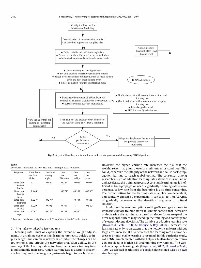
Fig. 2. A typical flow diagram for nonlinear multivariate process modelling using BPNN algorithm.

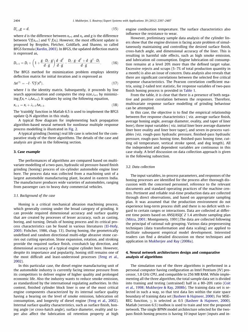
Table 1Correlation matrix for the two-pass finish honing process responses.

Response Liner boresurfacefinish

Liner borehoningangle

Linerborediameter

Linerboreovality

Linerboretaper

Liner boresurfacefinish

1 0.440⁄ 0.227⁄ �0.029 �0.067

Liner borehoningangle

0.440⁄ 1 0.277⁄ �0.102 �0.236⁄

Liner borediameter

0.227⁄ 0.277⁄ 1 �0.104 �0.123

Liner boreovality

�0.029 �0.102 �0.104 1 0.540⁄

Liner boretaper

�0.067 �0.236⁄ �0.123 0.540⁄ 1

⁄ Pearson correlation is significant at 0.01 confidence level (2-tailed test).

2400 I. Mukherjee, S. Routroy / Expert Systems with Applications 39 (2012) 2397–2407

2.1.1. Variable or adaptive learning rateLearning rate limits or expands the extent of weight adjust-

ments in a training cycle. A high learning rate reacts quickly to in-put changes, and can make networks unstable. The changes can betoo extreme, and cripple the network’s prediction ability. In thecontrary, if the learning rate is too low, the network training timeis substantially increased. A high learning rate is useful to acceler-ate learning until the weight adjustments begin to reach plateau.

However, the higher learning rate increases the risk that theweight search may jump over a minimum error condition. Thiscould jeopardize the integrity of the network and cause back-prop-agation learning to reach global optima. The consensus amongresearchers is that adaptive learning rates stabilize risk of failureand accelerate the training process. A constant learning rate is inef-ficient as back-propagation needs a gradually declining rate of con-vergence. A low rate from the beginning is also time consuming.The correct setting for the learning rate is application dependent,and typically chosen by experiment. It can also be time-varying,or gradually decreases as the algorithm progresses to optimalsolution.

In addition, determining optimal setting of learning rate is near toimpossible before training starts. It is in this context that increasingor decreasing the learning rate based on slope (flat or steep) of theerror response surface may speed up the training and convergenceof steepest decent algorithm. The variable or adaptive learning rate(Howard & Beale, 1998; Mukherjee & Ray, 2008c) increases thelearning rate only to an extent that the network can learn withoutlarge error increase. It also decreases the learning rate as error de-creases or until stable learning is resumed. In this particular study,A-L BPNN is implemented with the help of a built-in function, ‘train-gdx’ provided in Matlab 6.5 programming environment. The vari-able or adaptive learning rate (Hagan et al., 2002; Howard & Beale,1998) as selected at tth stage of epoch is determined based on twosimple steps,

Fig. 3. Progress of error performance measure using different algorithm for BPNN modelling.

I. Mukherjee, S. Routroy / Expert Systems with Applications 39 (2012) 2397–2407 2401

(i) calculating the current network error at ith stage of iteration,(ii) if ratio of new and old error exceeds a predefined value

ei(max), weights and biases of the network are discardedand reinitialized. In addition, the current learning rate isdecreased by a multiple of mi(decrease), or the new weights cal-culated are retained. If the new error is less than the olderror, the learning rate is increased by a multiple ofmi(increase).

In this study, the values of ei(max), mi(decrease), and mi(increase) areselected as 1.04, 0.7, and 1.05, respectively (Hagan et al., 2002;Howard & Beale, 1998).

2.2. The Levenberg–Marquardt algorithm-based BPNN (L–M BPNN)

The Levenberg–Marquardt (L–M) algorithm (Bazaraa, Sherali, &Shetty, 2004; Madsen, Nielsen, & Tingleff, 2004; Marquardt, 1963)

2402 I. Mukherjee, S. Routroy / Expert Systems with Applications 39 (2012) 2397–2407

outperforms simple gradient descent and many other conjugategradient methods in a wide variety of problems (Ampazis &Perantonis, 2000; Dombayci & Golcu, 2009; Nalbant, Gokkaya,Toktas, & Sur, 2009; Torrecilla, Otero, & Sanz, 2007). L–M is a blendof local search properties of Gauss–Newton with consistent errordecrease provided by gradient descent algorithm. The training offeed forward network based on L–M is considered as an uncon-strained optimization problem. The main disadvantage of L–Malgorithm is its increased memory requirement to calculate theJacobian matrix of the error function. Determining the inverse ofthe matrix with dimensions equal to the number of the weightsof neural network is cumbersome. Another disadvantage of L–Mis that it does not always guarantee global optimum for a uncon-strained optimization problem. The whole training process shouldbe restarted, when the solution is unacceptable. In case of gradientdescent algorithm, a momentum term is incorporated that helps toovershoot local minima. For a multiple output feed forward net-work, the mean square error E(t) objective function is expressed as,

EðtÞ ¼ 1Np

XN

i¼1

Xk¼p

k¼1

dik

� �2� yi

k

� �2� �

; ð7Þ

where yik is the kth desired or target output activation of ith training

sample. dik is the kth actual output from the ith training pattern. u is

the column vector containing all the weights, and thresholds of thenetwork.The main idea is to use second order Taylor series expan-sion method. By this approach, the local approximation of the costfunction is assumed quadratic, and expressed as

Eðut þ dutÞ ¼ EðutÞ þ rEðutÞT dut þ12

duTtr2EðutÞdut ; ð8Þ

whererE(ut) andr2E(ut) are the gradient vector and matrix of sec-ond order derivative of cost function, respectively. The optimal step(or Newton step) dut is obtained by the first optimality conditionand expressed as

dut ¼ �½r2EðutÞ��1rEðutÞ: ð9Þ

Due to the special form of Eq. (8), the second order derivative orHessian matrix can also be written as,

r2EðutÞ ¼ JTt Jt þ St

� �; ð10Þ

where Jtis the Jacobian matrix of first derivatives of the residuals

dik � yi

k

� �2, and St denotes the second order derivative information

ofr2E(ut). Ignoring the St term in Eq. (10) leads to Gauss–Newtonmethod. In actual, St approaches zero as the algorithm converges(Ampazis & Perantonis, 2000). Thus, Gauss–Newton method canachieve the quadratic convergence of Newton’s method by usingonly the information of its first derivatives. However, when algo-rithm is far away from optima, the term St cannot be negligible.Such approximation of the Hessian matrix can give poor resultswith slow convergence rate. The L–M method is based on theassumption that such an approximation is valid only within a trustregion with small radius. This type of approximation for the Hessianmatrix (Bazaraa et al., 2004) simplifies Eq. (10) as

r2EðutÞ ¼ JTt Jt þ lt I

� �; ð11Þ

Table 2Mean square error and network training time for BPNN algorithms.

BPNN algorithm

Gradient descent with momentum and adaptive learning (A-L)Levenberg–Marquardt (L–M)BFGS update Quasi-Newton (Q-N)

where I is the identity unit matrix and lt is a scalar that (indirectly)controls the size of the trust region. When lt = 0, the method be-comes equivalent to the Gauss–Newton method. Whereas, for largelt, the L–M algorithm tends towards steepest descent algorithm. Acommon approach to implement L–M for training of neural net-works is by selection a small l0. In subsequent iteration, lt canbe adjusted according to following logic:

(i) If a successful step is taken [i.e. E(ut + dut) < E(ut)], then lt isdecreased by a factor of 0.1. This will lead the iterationtowards Gauss–Newton direction.

(ii) if the step is unsuccessful [e.g. E(ut + dut) > E(ut)], then lt isincreased by a factor 10, until a successful step can beobtained.

It has been shown that L–M method does not guarantee globaloptimal and it is just a heuristic, that works extremely well in prac-tical problems (Bazaraa et al., 2004). The main drawback of this algo-rithm is its computational complexity to calculate matrix inversionwith variable size of few thousand. Generally, inverse of Hessian isimplemented by pseudo-inverse method or singular value decom-position approach.

The ‘trainlm’ function in Matlab 6.5 is used to implement the L–M algorithm-based BPNN for this particular study. The value of l0

is selected as 0.001 and maximum value of lt is assumed to be 1010

for this study.

2.3. Boyden, Fletcher, Goldfarb and Shanno (BFGS) update Quasi-Newton algorithm-based BPNN (Q-N BPNN)

The gradient descent search requires only information of firstpartial derivative but can often gives poor numerical performance(Rardin, 2003). Gauss–Newton (G–N) algorithm yields improvedconvergence but require second derivative information and alsoto solve system of linear equations in each step.

Quasi-Newton algorithm (Brezinski, 2003; Oren, 1976;Robitaille, Marcos, Veillejte, & Payre, 1996; Shanno & Kettler,1970; Xu & Zhang, 2001) is a blend of these two algorithms, andis based on the concept of conjugacy. If the objective function isunconstrained and quadratic in nature, then searching alone theconjugate directions of Hessian matrix can give a minimum pointin n steps.

The Newton step size (Dx) for a second order Taylor seriesapproximation of f(x) at any current point xi is obtained from theequation

HðxiÞDx ¼ �rf ðxiÞ: ð12Þ

Dx is further used to calculate xi+1, and the equation is

xiþ1 ¼ xi þ Dx: ð13Þ

The search will continue until krf(xi)k < e, where e is the stoppingcriteria or tolerance. In this study, e is selected as 10�6.

Assuming that the Hessian matrix is non-singular, Eq. (12) canalso be rewritten as

Dx ¼ �HðxiÞ�1rf ðxiÞ; ð14Þ

where Di = H(xi)�1 is so-called the ‘deflection matrix’.

Mean square errors Network training time (sec) per epoch

0.3186 0.002030.2117 0.10220.2356 0.0234

Fig. 4. Plot of actual and predicted test sample responses using (a) A-L-based BPNN, (b) L–M-based BPNN, (c) BFGS update Q-N-based BPNN.

I. Mukherjee, S. Routroy / Expert Systems with Applications 39 (2012) 2397–2407 2403

The deflection matrix should assure improved directions bykeeping Di positive definite for a minimization problem. Various

updating formula exist, that can meet the Quasi Newton require-ment. One such expression is,

2404 I. Mukherjee, S. Routroy / Expert Systems with Applications 39 (2012) 2397–2407

D�iþ1g ¼ d; ð15Þ

where d is the difference between xi+1 and xi, and g is the differencebetween rf(xi+1) and r f(xi). However, the most efficient update isproposed by Broyden, Fletcher, Goldfarb, and Shanno, so calledBFGS formula (Rardin, 2003). In BFGS, the updated deflection matrixis expressed as,

Diþ1 ¼ Di þ 1þ g � Di � gd � g

� d � dT

d � g �Di � g � dT þ d � gT � Di

d � g : ð16Þ

The BFGS method for minimization problem employs identitydeflection matrix for initial iteration and is expressed as

Dxð1Þ ¼ �I � rf ðx0Þ; ð17Þ

where I is the identity matrix. Subsequently, it proceeds by linesearch approximation and computes the step size,ki+1 by minimiz-ing f(xi + kiDxi+1). It updates by using the following equation,

xiþ1 ¼ xi þ kiþ1Dxiþ1: ð18Þ

The ‘trainbfg’ function in Matlab 6.5 is used to implement the BFGSupdate Q-N algorithm in this study.

A typical flow diagram for implementing back propagationalgorithm-based neural network for nonlinear multiple responseprocess modelling is illustrated in Fig. 2.

A typical grinding (honing) real life case is selected for the com-parative study of the three algorithms. The details of the case andanalysis are given in the following section.

3. Case example

The performances of algorithms are compared based on multi-variate modelling of a two-pass, hydraulic oil pressure-based finishgrinding (honing) process of six-cylinder automobile engine linerbore. The process data was collected from a machining unit of alargest automobile manufacturing plant, located in eastern India.The manufacturer produces wide varieties of automobiles, rangingfrom passenger cars to heavy duty commercial vehicles.

3.1. Background of the case

Honing is a critical mechanical abrasion machining process,which generally coming under the broad category of grinding. Itcan provide required dimensional accuracy and surface qualitythat are created by processes of lesser accuracy, such as casting,boring, and turning. Details of honing process and its critical pro-cess characteristics can be found in various literatures (El-Hofy,2005; Fishcher, 1986, chap. 13). During honing, the geometricallyundefined and random directional multi-edge abrasive stone car-ries out cutting operation. Stone expansion, rotation, and strokingprovide the required surface finish, crosshatch lay direction, anddimensional accuracy of a typical engine cylinder bore. However,despite its importance and popularity, honing still remains one ofthe most difficult and least-understood processes (Feng et al.,2002).

In this particular case, the diesel engine manufacturing unit ofthe automobile industry is currently facing intense pressure fromits competitors to deliver engine of higher quality and prolongedeconomic life. Also the industry wants to reduce smoke emission,as standardized by the international regulating authorities. In thiscontext, finished cylinder block liner is one of the most criticalengine components characterized by its internal surface qualityhaving a bearing on the level of smoke emission, lubrication oilconsumption, and longevity of diesel engine (Feng et al., 2002).Internal surface quality characteristics, such as surface finish, hon-ing angle (or cross-hatch angle), surface diameter, ovality and ta-per also affect the lubrication oil retention property at high

engine combustion temperature. The surface characteristics alsoinfluence the resistance to wear.

However, preliminary sample data analysis of the cylinder lin-ers show that the engine division is facing acute problem of simul-taneously maintaining and controlling the desired surface finish,cross-hatch angle, and dimensional accuracy of the liner. This isresulting in harmful side effects, such as high smoke emission,and lubrication oil consumption. Engine lubrication oil consump-tion remains at a level 20% more than the defined target value.Excessive rejects and scraps (5–7% of total production quantity ina month) is also an issue of concern. Data analysis also reveals thatthere are significant correlations between the selected five criticalresponse characteristics. The Pearson correlation coefficient ma-trix, using 2-tailed test statistic, for response variables of two-passfinish honing process is provided in Table 1.

From the table, it is clear that there is a presence of both nega-tive and positive correlation between the responses. Therefore,multivariate response surface modelling of grinding behaviourcan be attempted.

In this case, the objective is to find the empirical relationshipbetween five response characteristics ( viz. average surface finish,average honing angle, average diameter, ovality, and taper of linerbore), three input variables ( viz. initial liner bore average diameterliner bore ovality and liner bore taper), and seven in-process vari-ables (viz. rough-pass hydraulic pressure, finished-pass hydraulicpressure, rough-pass honing time, finished-pass honing time, cut-ting oil temperature, vertical stroke speed, and dog length). Allthe independent and dependent variables are continuous in thiscase study. A brief discussion on data collection approach is givenin the following subsection.

3.2. Data collection

The input variables, in-process parameters, and responses of thehoning processes are identified for the process after thorough dis-cussion with the concerned personnel, reference to the relevantdocuments and standard operating practices of the machine cen-tres. Pertinent and reliable real-time production data are collectedthrough direct observations, and based on appropriate samplingplan. It was assumed that the production environment do notexperience long-term process shift and there is no deficit with re-gard to certain ranges or interactions. Data are collected at differ-ent time points based on ANSI/ASQC Z 1.4 attribute sampling plan(Mitra, 2001; Montgomery, 1991).The data are collected followingthe principal of rational sub grouping. Various data prepossessingtechniques (data transformation and data scaling) are applied tofacilitate subsequent empirical model development. Interestedreaders can find a detailed discussion on these techniques andapplication in Mukherjee and Ray (2008a).

4. Neural network architectures design and comparativeanalysis of algorithms

The simulation run of the three algorithms is performed in apersonal computer having configuration as Intel Pentium (IV) pro-cessor, 1.8 GHz CPU, and compatible to 256 MB RAM. While imple-menting all the three algorithm, the total sample data set is dividedinto training and testing (untrained) half in a 80–20% ratio (Coitet al., 1998; Mukherjee & Ray, 2008b). The training data set is se-lected in such a way, so that test data lies within the state spaceboundary of training data set (Basheer & Hajmeer, 2000). For MSE-REG function, ci is selected as 0.5 (Basheer & Hajmeer, 2000).Matlab (version 6.5) toolbox is used to train and test the proposednetwork. The single BPNN model architecture selected for the two-pass finish honing process is having 10 input layer (inputs and in-

Table 3Correlation coefficient (r) of predicted outputs with actual outputs using test sample.

Algorithm Avg.surfacefinish (Y1)

Avg.honingangle (Y2)

Avg. linerborediameter(Y3)

Linerboreovality(Y4)

Linerboretaper(Y5)

ResponsesA-L BPNN 0.834 0.715 0.779 0.247 0.042L–M BPNN 0.845 0.625 0.341 0.283 0.42BFGS

updateQ-NBPNN

0.818 0.446 0.687 0.376 0.193

Table 4aSummary statistics of r-values.

Summary statistic Count Average Variance

A-L BPNN 5 0.5234 0.1266L–M BPNN 5 0.5028 0.0533BFGS update Q-N BPNN 5 0.5040 0.0621Avg. surface finish (Y1) 3 0.8323 0.0001Avg. honing angle (Y2) 3 0.5953 0.0187Avg. diameter (Y3) 3 0.6023 0.0533Ovality (Y4) 3 0.3020 0.0044Taper (Y5) 3 0.2183 0.0362

Table 4bA two-factor analysis of variance without replication using r-values.

Source ofvariation

Sum ofsquare

Degree offreedom

Mean sumof square

F-calculated

P-value

F-tabulated

Algorithms 0.0013 2 0.0007 0.023⁄⁄ 0.976⁄⁄ 4.458Response

variables(Y’s)

0.7441 4 0.1860 6.629⁄ 0.011⁄ 3.837

Error 0.2244 8 0.0281Total 0.9699 14

⁄ Statistically significant at a = 0.05 (level of significance).⁄⁄ Not statistically significant at a = 0.05 (level of significance).

Table 5aError performance measures for individual responses using test sample data and A-LBPNN.

Trainingalgorithm

Differentmeasuresof error

Based on test sample data

Avg.surfacefinish(Y1)

Avg.honingangle(Y2)

Avg. linerborediameter(Y3)

Linerboreovality(Y4)

Linerboretaper(Y5)

A-L BPNN AAD 0.5048 1.1333 1.5834 2.5112 3.4866MSE 0.1474 0.7404 0.3757 0.2541 0.0117RMSE 0.3839 0.8605 0.6129 0.5041 0.1081MPE (%) 0.6893 0.8422 4.9332 1.3916 2.5700MAPE (%) 0.6903 0.8304 0.7643 0.8689 0.9782MRE (%) 1.2856 2.6991 4.1717 5.9822 8.0052

Table 5bError performance measures for individual responses using test sample data and L–MBPNN.

Trainingalgorithm

Differentmeasuresof error

Based on test sample data

Avg.surfacefinish(Y1)

Avg.honingangle(Y2)

Avg. linerborediameter(Y3)

Linerboreovality(Y4)

Linerboretaper(Y5)

L–MBPNN

AAD 0.4199 1.0531 1.8424 2.7004 3.4103MSE 1.1260 0.9792 0.0145 0.2612 0.0080RMSE 1.0611 0.9895 0.1204 0.5111 0.0897MPE (%) 0.1313 1.5917 0.2107 1.4178 1.1153MAPE (%) 0.4619 0.5638 0.6968 0.7645 0.7683MRE (%) 2.0218 4.0437 6.0656 8.0875 10.1093

Table 5cError performance measures for individual responses using test sample data and BFGSupdate Q-N BPNN.

Trainingalgorithm

Differentmeasuresof error

Based on test sample data

Avg.surfacefinish(Y1)

Avg.honingangle(Y2)

Avg. linerborediameter(Y3)

Linerboreovality(Y4)

Linerboretaper(Y5)

BFGSupdateQ-NBPNN

AAD 0.5157 1.3498 1.8358 2.5695 3.4453MSE 1.0688 1.1275 0.0146 0.2612 4.3668RMSE 1.0338 1.0618 0.1211 0.5111 2.0897MPE (%) 0.5969 1.6419 5.1572 0.1608 1.3165MAPE (%) 0.6472 0.8262 0.7701 0.7865 0.8306MRE (%) 2.1858 4.3717 6.5576 8.7434 10.9293

I. Mukherjee, S. Routroy / Expert Systems with Applications 39 (2012) 2397–2407 2405

process parameters), 5 output layer (responses), and 20 neurons insingle hidden layer. Selection of number of hidden layer and neu-rons in any particular hidden layer is purely based on trial runs,and can be debated. The network adopted for this comparativestudy is purely based on trial-by-trial method. Different algorithmswith varied number of neurons are tested to achieve a level ofmodel accuracy. There is no single approach that can be used todetermine the best network for all situations. The data analysis

and interpretation of results after training and testing of all thenetworks is given below.

4.1. Training and testing of network architectures

The network is trained in batch training mode, and the progressof the performance measure, mean square error, for A-L BPNN,L–M BPNN, and BFGS update Q-N BPNN algorithm is shown inFig. 3(a–c).

4.2. Comparative results and analysis

Table 2 provides the mean square error measure, and networktraining time per epoch for BPNN model using the three differentalgorithms.

From Table 2 and Fig. 3, it is clear that back propagation learn-ing using L–M algorithm converges faster than A-L and Q-N algo-rithm. The training MSE values also indicate that L–M BPNNprovides a more accurate nonlinear predictive model, followedby Q-N method, and lastly A-L BPNN. However, A-L BPNN takesthe minimum time for network training. BFGS update Q-N requiredabout 10 times and L–M requires about 50 times more computa-tional time than A-L-based BPNN.

Fig. 4(a–c) provides the plot of actual and predicted test sampleresponse for the three different algorithms.

Table 3 provide the correlation co-efficient (r) for all the five re-sponses using test sample data and any specific algorithm.

The individual r-values of five responses do not provide a clearindication about the superiority of any particular algorithm. A-LBPNN predicts Y1, Y2, and Y3 comparatively better than L–M orQ-N-based BPNN. L–M predicts Y1 and Y5 better than A-L BPNNand Q-N BPNN.

Statistical analysis can provide better insight to identify if thereis any significant difference in the predictive performance of thesethree algorithms. A two-factor analysis of variance (ANOVA) with-

Table 6A brief summary of the training algorithm.

Intrinsic detailsnalgorithm A-L BPNN L–M BPNN BFGS update Q-N BPNN

Optimization technique Gradient descent search Blend of gradient descent and Gauss–Newtonbased search

Conjugate gradient based search and BFGS updaterule for deflection matrix

Performance function A modified performance, socalled MSEREG

Mean square error Mean square error

Mode of training Batch Batch BatchConvergence Fast Fastest FasterNetwork training time per

EpochMinimum Maximum Medium

Rate/size Variable learning rate A scalar, lt, that (indirectly) controls the sizeof the trust region

Step size and deflection matrix

Memory storagerequirement

Small Large Large

Suitability for multipleresponse problem

Suitable Suitable Suitable

Online dynamic processcontrol

Best as learning is very fast Can be used if computational speed oflearning is high

Can be used if computational speed of learning is high

2406 I. Mukherjee, S. Routroy / Expert Systems with Applications 39 (2012) 2397–2407

out replication is performed on the r-values. The summary statis-tics and two-way ANOVA results are provided in Tables 4a and 4b.

The two-way ANOVA analysis indicates that the correlation co-efficient (r) does not show a significant difference when differentalgorithms are used predicting the given set of test data. In otherwords, all the three algorithms (A-L BPNN, L–M BPNN, and BFGSupdate Q-N BPNN) are having same efficiency to predict test dataset. However, the statistically significant result on r-values for re-sponse variables (Y’s) is obvious, as MSE values will vary for differ-ent Y’s. However, seeing the comparative r-values for Y1, Y2 and Y3,and time taken to training the network, A-L-based BPNN can bepreferred. In addition, understanding the A-L BPNN may be easieras compared to L–M and BFGS update Q-N-based BPNN. In a dy-namic online process control environment, A-L BPNN may bepreferred.

Tables 5a–5c also provides various error performance measuresfor each responses, using the test sample data. The different errormeasures reported in the table are expressed as,

Average Absolute Deviation : AAD¼ 1N

XN

t¼1

jyðtÞ � ydðtÞj; ð19Þ

Mean Square Error : MSE¼ 1N

XN

t¼1

ðyðtÞ � ydðtÞÞ2; ð20Þ

Root Mean Square Error : RMSE¼ffiffiffiffiffiffiffiffiffiffiMSEp

; ð21Þ

Mean Percentage Error : MPE¼ 1N

XN

i¼1

½yðtÞ � ydðtÞ�ydðtÞ

; ð22Þ

Mean Absolute Percentage Error : MAPE¼ 1N

XN

i¼1

½yðtÞ � ydðtÞ�ydðtÞ

��������; and ð23Þ

Mean Relative Error : MRE¼ 100N

XN

i¼1

jyðtÞ � ydðtÞjydðtÞ

: ð24Þ

Here, y(t) is the actual output, yd(t) is the predicted output of thetrained network, and N is the total number of patterns used fortraining.

All the measures are provided as there is no single consensus onwhich measure is most appropriate to compare different algo-rithms. Based on the overall theoretical understanding and caseanalysis using the three algorithms, a summary is provided inTable 6.

5. Conclusions

In this paper, two different training algorithms, viz. Levenberg–Marquardt (L–M), and BFGS update Quasi-Newton is comparedwith gradient descent algorithm to develop a BPNN model fornonlinear modelling multiple response honing process. The

comparative analysis is based on actual production data collectedover a period of time. The key finding that came out from this studyis:

(i) L–M and Q-N algorithm-based BPNN networks areequally efficient as A-L algorithm-based BPNN networkto predict the behaviour of multiple response grindingprocess.

(ii) L–M algorithm has fastest network convergence rate, fol-lowed by BFGS update Q-N and A-L algorithm.

(iii) A-L-based BPNN learns faster than BFGS update Q-N, and L–M takes the maximum time for training, and

(iv) A-L algorithm is relatively easy-to-understand and imple-ment as compared to L–M or BFGS update Q-N algorithmfor online process control.

The future scopes of research are:

(i) Verifying the suitability of L–M and BFGS update Q-N algo-rithm for predicting varied other cutting situations.

(ii) Incorporating experimental data for robust variability mod-elling and compare the algorithms performances.

(iii) Develop a framework to determine optimal network config-uration for such type of comparative studies.

Acknowledgements

The authors of this paper would like to acknowledge the sup-port and assistance provided for data collection by Quality Assur-ance (Engine Division), and Production (Engine Division)Department of Tata Motors Ltd., Jamshedpur, India.

References

Ampazis, N., & Perantonis, S. J. (2000). Levenberg–Marquardt algorithm withadaptive momentum for the efficient training of feedforward networks. InProceedings of IEEE & INNS international joint conference on neural networks,IJCNN 2000, paper no. NN0401, Como, Italy, (CD proceedings) (pp. 126–131).

Basheer, I. A., & Hajmeer, M. (2000). Artificial neural networks: Fundamentals,computing, design, and application. Journal of Microbiological Methods, 43, 3–31.

Bates, D. M., & Watts, D. G. (1988). Nonlinear regression analysis and its applications.New York: John Wiley and Sons.

Bazaraa, M. S., Sherali, H. D., & Shetty, C. M. (2004). Nonlinear programming. Theoryand algorithms (2nd ed., ). India: Wiley.

Box, G. E. P., & Draper, N. R. (1987). Empirical model-building and response surface.New York: John Willey and Sons.

Brezinski, C. (2003). A classification of quasi-Newton methods. NumericalAlgorithms, 33, 123–135.

Chen, H., Lin, J., Yang, Y., & Tsai, C. (2010). Optimization of wire electrical dischargemachining for pure tungsten using a neural network integrated simulatedannealing approach. Expert Systems with Applications, 37, 7147–7153.

I. Mukherjee, S. Routroy / Expert Systems with Applications 39 (2012) 2397–2407 2407

Chen, Y. T., & Kumara, S. R. T. (1998). Fuzzy logic and neural network for design ofprocess parameters: A grinding process application. International Journal ofProduction Research, 36(2), 395–415.

Choi, T. J., Subrahmanya, N., Li, H., & Shin, C. Y. (2008). Generalized practical modelsof cylindrical plunge grinding processes. International Journal of Machine Toolsand Manufacture, 48, 61–72.

Coit, D. W., Jackson, B. T., & Smith, A. E. (1998). Static neural network processmodels: Considerations and case studies. International Journal of ProductionResearch, 36(11), 2953–2967.

Cus, F., Zuperl, U., & Milfelner, M. (2006). Dynamic neural network approach for toolcutting force modelling of end milling operations. International Journal ofGeneral Systems, 35(5), 603–618.

Dombayci, O. A., & Golcu, M. (2009). Daily means ambient temperature predictionusing artificial neural network method: A case study of Turkey. RenewableEnergy, 34(4), 1158–1161.

El-Hofy, H. (2005). Advanced machining processes: Nontraditional and hybridmachining processes. New York: MacGraw-Hill.

Farago, F. T. (1976). Abrasive methods engineering. NY: Industrial Press Inc.Feng, C., Wang, X., & Yu, Z. (2002). Neural networks modelling of honing surface

roughness parameter defined by ISO 13565. SIAM Journal of ManufacturingSystems, 21(8), 1–35.

Fishcher, H. (1986). In R. I. King & R. S. Hahn (Eds.), Honing in handbook of moderngrinding technology (pp. 301–336). New York: Chapman and Hall.

Fu, L. (2003). Neural network in computer intelligence. India: Tata McGraw Hill.Govindhasamy, J. J., MacLoone, S. F., Irwin, G. W., French, J. J., & Doyle, R. P. (2005).

Neural modelling, control and optimization of an industrial grinding process.Control Engineering Practice, 13, 1243–1258.

Haber, R. E., & Alique, A. (2003). Intelligent process supervision for predicting toolwear in machining processes. Mechatronics, 13, 825–849.

Hagan, M. T., Demuth, H. B., & Beale, M. (2002). Neural network design. India:Thomson Learning.

Howard, D., & Beale, M. (1998). Neural network toolbox: For use with Matlab; user’sGuide, version 3. USA: The Mathworks Inc.

Jain, R. K., Jain, V. K., & Kalra, P. K. (1999). Modelling of abrasive flow machiningprocess: A neural network approach. Wear, 231, 242–248.

Krajnik, P., Kopac, J., & Sluga, A. (2005). Design of grinding factors based on responsesurface methodology. Journal of Materials Processing Technology, 162–163. 629-636.

King, R. I., & Hahn, R. S. (1986). Handbook of modern grinding technology. New York:Chapman and Hall.

Kumar, S., & Choudhury, S. K. (2007). Prediction of wear and surface roughness inelectro-discharge diamond grinding. Journal of Materials Processing Technology,191, 206–209.

Kwak, J. (2005). Application of Taguchi and response surface methodologies forgeometric error in surface grinding process. International Journal of MachineTools and Manufacturing, 45, 327–334.

Luong, L. H. S., & Spedding, T. A. (2002). A neural-network system for predictingmachining behaviour. Journal of Materials Processing Technology, 52, 585–591.

Madsen, K., Nielsen, H. B., & Tingleff, O. (2004). Methods for non-linear least squaresproblems (2nd ed.). Technical University of Denmark.

Maksoud, T. M. A., & Atia, M. R. (2004). Review of intelligent grinding and dressingoperations. Machine Science and Technology, 8(2), 263–276.

Malkin, S. (2007). Thermal analysis of grinding. Annals of CIRP, 56(2), 760–782.Malkin, S. (1984). Grinding of metals: Theory and application. Journal of Applied

Metalwork, 3, 95–109.Markos, S., Viharos, Zs. J., & Monostori, L. (1998). Quality-oriented, comprehensive

modelling of machining processes. In 6th ISMQC IMEKO symposium on metrologyfor quality control in production (pp. 67–74).

Marquardt, D. W. (1963). An algorithm for least-squares estimation of nonlinearparameters. Journal Society Industrial Applied Mathematics, 11(2), 431–441.

Mitra, A. (2001). Fundamentals of quality control and improvement (2nd ed.). India:Pearson Education Asia, Inc.

Montgomery, D. C. (1991). Introduction to statistical quality control (2nd ed.). NewYork: John Wiley and Sons.

Montgomery, D. C. (2001). Design and analysis of experiment (5th ed.). New York:Wiley and sons Inc.

Montgomery, D. C., & Peck, E. A. (1992). Introduction to linear regression analysis (2nded.). New York: John Wiley and Sons, Inc.

Moulik, P. N., Yang, H. T. Y., & Chandrasekhar, S. (2001). Simulation of thermalstresses due to grinding, international. Journal of Mechanical Society, 43,831–851.

Mukherjee, I. (2007). Modelling and optimization of abrasive metal cutting processes.Ph.D. Thesis, Department of Industrial Engineering and Management. IndianInstitute of Technology, Kharagpur, India.

Mukherjee, I., & Ray, P. K. (2006). A review of optimization techniques in metalcutting processes. International Journal of Computers and Industrial Engineering,50, 15–34.

Mukherjee, I., & Ray, P. K. (2008a). A systematic solution methodology forinferential multivariate modelling of industrial grinding process. InternationalJournal of Materials Processing Technology, 196, 379–392.

Mukherjee, I., & Ray, P. K. (2008b). Technology management of grinding processusing quality control methods: A multivariate regression and neural networkapplication. In Innovation and Technology Management Advanced Research Series(pp. 238–246). India: Macmillan.

Mukherjee, I., & Ray, P. K. (2008c). A modified tabu search strategy for multiple-response grinding process optimization. International Journal of IntelligentSystems Technologies and Applications, 4(1/2), 97–122.

Nalbant, M., Gokkaya, H., Toktas, I., & Sur, G. (2009). The experimental investigationof the effects of uncoated, PVD- and CVD-coated cemented carbide inserts andcutting parameters on surface roughness in CNC turning and its predictionusing artificial neural networks. Robotics and Computer-IntegratedManufacturing, 25(1), 211–223.

Oren, S. S. (1976). On quasi-Newton and pseudo-Newton algorithms. Journal ofOptimization Theory and Applications, 20(2), 155–170.

Petri, K. L., Billo, R. E., & Bidanda, B. (1998). A neural network process model forabrasive flow machining operations. Journal of Manufacturing Systems, 17(1),52–64.

Rardin, R. L. (2003). Optimization in operations research. India: Pearson Education.Rencher, A. C. (1995). Method of multivariate analysis. USA: John Wiley and Sons, Inc.Rencher, A. C. (1998). Multivariate statistical inference and applications. New York:

John Wiley and Sons, Inc.Rumelhart, D. E., Hilton, G. E., & Williams, R. J. (1986). Learning representations by

back-propagating errors. Nature, 323(9), 533–536.Robitaille, B., Marcos, B., Veillejte, M., & Payre, G. (1996). Modified quasi-Newton

methods for training neural networks. Computers and Chemical Engineering,20(9), 1133–1140.

Rowe, B. W., Yan, L. I., lnasaki, I., & Malkin, S. (1994). Applications of artificialintelligence in grinding. Annals of CIRP, 43(2), 521–531.

Sathyanarayanan, G., Lin, I. J., & Chen, M. (1992). Neural network modelling andmultiobjective optimization of creep feed grinding of superalloys. InternationalJournal of Production Research, 30(10), 2421–2438.

Sedighi, M., & Afshari, D. (2010). Creep feed grinding optimization by an integratedGA-NN system. Journal of Intelligent Manufacturing, 21(6), 657–663.

Shaji, S., & Radhakrisnan, V. (2003). Analysis of process parameters in surfacegrinding with graphite as lubricant based on Taguchi method. Journal ofMaterial Processing Technology, 1–9.

Shanno, D. F., & Kettler, P. C. (1970). Optimal conditioning of quasi-newtonmethods. Mathematics of Computation, 24(111), 657–664.

Shin, Y. C., & Vishnupad, P. (1996). Neuro-fuzzy control of complex manufacturingprocesses. International Journal of Production Research, 34(12), 3291–3309.

Sorensen, P. H., Norgaard, M., Ravn, O., & Poulsen, N. K. (1999). Implementationof neural network based non-linear predictive control. Neurocomputing, 28,37–51.

Tawakoli, T., Rabiey, M., & Lewis, M. (2009). Neural Network prediction of drygrinding by CBN grinding wheel using special conditioning. International Journalof Materials and Product Technology, 35(1/2), 118–133.

Torrecilla, J. S., Otero, L., & Sanz, P. D. (2007). Optimization of an artificial neuralnetwork for thermal/pressure food processing: Evaluation of trainingalgorithms. Computers and Electronics in Agriculture, 56, 101–110.

Tsai, K., & Wang, P. (2001). Predictions of surface finish in electrical dischargemachine based upon neural network models. International Journal of MachineTools and Manufacture, 41, 1385–1403.

Urbaniak, M. (2004). Evaluation system for the cutting properties of grindingwheels. Proceedings of the Institution of Mechanical Engineers, Part B: Journal ofEngineering Manufacture, 218(11), 1491–1498.

Vafaeesefat, A. (2009). Optimum creep feed grinding process conditions for rene 80supper alloy using neural network. International Journal of Precision Engineeringand Manufacturing, 10(3), 5–11.

Wasserman, P. D. (1993). Advanced methods in neural computing. New York: VanNostrand Reinhold.

Widrow, B., & Lehr, M. A. (1990). 30 Years of adaptive neural networks: Perceptron,Madaline, and back propagation. Proceedings of IEEE, 78(9), 1415–1442.

Xu, C., & Zhang, J. (2001). A survey of quasi-Newton equations and quasi-newtonmethods for optimization. Annals of Operations Research, 103, 213–234.

Zadeh, L. A. (1965). Fuzzy sets. Information and Control, 8, 338–353.Zhang, H. C., & Huang, S. H. (1995). Application of neural network in manufacturing

– a state of art survey. International Journal of Production Research, 33(3),705–728.