ARTICLE

Comparing the efficacy of linear programming models I and IIfor spatial strategic forest managementAndrew B. Martin, Evelyn Richards, and Eldon Gunn

Abstract: Contemporary strategic forest management goals have become increasingly complex in spatial definition and scale.For example, the Canadian Council of Forest Ministers Criteria and Indicators (CCFM C&I) includes metrics that are expressed atmultiple levels of spatial resolution such as ecodistricts, watersheds, and vegetative communities. Supporting these criteria withaspatial models is sometimes difficult, and results are often not transferable to the actual forest. We describe a spatial Model Istand and prescription-based strategic forest planning model that includes spatial metrics in a realistic sized problem. Wecompare its formulation, capabilities, and computational efficiency with a Model II formulation using a case study on NovaScotia’s Crown Central Forest. We demonstrate that the spatial Model I is better suited to support strategic forest managementwhen spatial criteria are included.

Key words: forest management, strategic planning, linear programming, ecosystem-based management, spatial constraints.

Résumé : Les objectifs de l’aménagement forestier stratégique moderne sont devenus de plus en plus complexes en termesd’échelle et de définition spatiales. À titre d’exemple, les critères et indicateurs du Conseil canadien des ministres des forêts(C et I du CCMF) comportent des métriques associées a différentes résolutions spatiales, telles que les écodistricts, les bassinsversants et les communautés végétales. Il est parfois difficile d’intégrer ces critères dans des modèles aspatiaux et il est souventimpossible d’appliquer les résultats en forêt. Nous décrivons un modèle spatial I, un modèle de planification forestière straté-gique fondé sur le peuplement et les prescriptions et qui inclut des métriques spatiales dans un problème dont la taille estréaliste. Nous comparons sa formulation, ses capacités et son efficacité computationnelle a celles d’une formulation de Modèle IIen ayant recours a une étude de cas dans les forêts de la Couronne du centre de la Nouvelle-Écosse. Nous démontrons que lemodèle spatial I convient mieux pour appuyer l’aménagement forestier stratégique lorsque des critères spatiaux sont inclus.[Traduit par la Rédaction]

Mots-clés : aménagement forestier, planification stratégique, programmation linéaire, gestion écosystémique, contraintesspatiales.

1. IntroductionForest strategic planning addresses sustainability of forests

with respect to environmental, economic, and social dimensions.In the Montreal Process, 12 member countries, accounting for 90%of the world’s temperate and boreal forest, defined criteria andindicators for sustainable forest management (Montreal Process1998). In Canada, the Canadian Council of Forest Ministers Criteriaand Indicators (CCFM C&I) (CCFM 2003) define the principles thatforest management strategy must address to be sustainable. Asone might expect, many of these have spatial specifications. Forexample, a goal such as forest contribution to water quality ismeasured at a watershed scale, whereas ecosystem diversity ismeasured at an ecodistrict scale. In provincial jurisdictions, man-agement strategies are determined based upon what the C&Imean in local forest and policy contexts. Ecosystem-based man-agement (EBM) (Stewart and Neilly 2008; Pretzsch et al. 2008) isused as the framework around which strategy is constructed sothat it is regionally relevant and nationally coherent.

Analyzing impacts of proposed plans on long-term sustainabil-ity of large forests is a daunting task, and analysts need decisionsupport systems to facilitate the process (Seely et al. 2004). These

decision support systems are usually powered by optimizationand (or) simulation models of various types that project the im-pact of management actions on the forest over time. With manyplanning periods, stand types, and management options, solvingoptimization models of the full spectrum of key economic andenvironmental metrics is challenging. Furthermore, when objec-tives, constraints, or goals have spatial dimensions, the computa-tional challenge increases significantly.

Mathematical optimization models that guarantee feasible andoptimal solutions such as linear programming (LP) models areextremely useful for examining trade-offs between managementchoices. If solving to optimality is not attainable or necessary,then approximate methods such as heuristics may be used tosolve the model (Pukkala 2013; see also the commercial Patch-works software package (Rouillard and Moore 2008)). Simulationsystems do not optimize but can generate and assess proposedsolutions. For example, Nelson (2003) created a forest-level spatialplanning simulator. Simulation is often combined with linear ormixed integer models to generate solutions (Gustafson et al. 2006).

Hierarchical forest management (HFM) (Bitran and Hax 1977) isa system that organizes management into separate but linkedstrategic, tactical, and operational planning phases. The HFM sys-

Received 25 March 2016. Accepted 10 August 2016.

A.B. Martin and E. Gunn.* Department of Industrial Engineering, Dalhousie University, Halifax, NS, Canada.E. Richards. Faculty of Forestry and Environmental Management, University of New Brunswick, Fredericton, NB, Canada.Corresponding author: Evelyn Richards (email: ewr@unb.ca).*Deceased.Copyright remains with the author(s) or their institution(s). Permission for reuse (free in most cases) can be obtained from RightsLink.

16

Can. J. For. Res. 00: 16–27 (0000) dx.doi.org/10.1139/cjfr-2016-0139 Published at www.nrcresearchpress.com/cjfr on 25 August 2016.

Can

. J. F

or. R

es. D

ownl

oade

d fr

om w

ww

.nrc

rese

arch

pres

s.co

m b

y U

nive

rsity

of

Tor

onto

on

11/0

7/16

For

pers

onal

use

onl

y.

tems typically remove spatial considerations from the strategicplanning phase and use an aspatial model to determine estimatesof sustainable flows of timber over multiple forest rotations.These estimated flows are inputs to the subsequent tactical plan-ning phase where, on a shorter time horizon and fewer planningperiods, spatial goals, as well as other tactical issues, are ad-dressed. This produces revised estimates of sustainable flows thatare then used as inputs to the strategic planning process. Thiscycle is repeated until a defensible strategy is determined.

By using disaggregated models, HFM has the potential to pro-duce suboptimal solutions, and there are uncertainties in predict-ing long-term sustainability when spatial considerations areassessed at shorter time horizons (Weintraub and Cholaky 1991).Gunn (2010) draws attention to the difficulties in interpretingoutputs from strategic aspatial planning models as inputs to atactical planning phase. The specific structure of an optimal solu-tion from an aspatial strategic model in HFM may bear little rela-tion to an optimal spatial solution, and Gunn (2010) concludesthat a common practice of implementing details of the aspatialsolution is “highly questionable”. Paradis et al. (2013) observedthat when using HFM, systematic disconnectedness betweenplanned and implemented forest management activities may re-sult in a significant divergence between planned and actual forestcondition over time, compromising credibility and performanceof the forest management planning process. Gunn (2010) also sug-gested that a spatial Model I formulation can contain the elementsfor better HFM and strategic forest management planning.

Linear programming models provide an unambiguous guaran-tee of feasibility and optimality and have been successfully ap-plied to large-scale problems in many fields. Two LP model forms,known as Model I and Model II (Johnson and Scheurman 1977), arewell-known formulations that have been widely used in strategicforest planning (Martell et al. 1998). Both models allow a managerto explore the effects of a suite of silvicultural activities on eco-nomic returns and future forest condition. However, they arequite different in structure. Model I is stand based and, in thissense, is a spatial model. It retains stand spatial resolution in thelandbase with decision variables that choose prescriptions to beapplied to specific stands. These prescriptions are a set of silvicul-tural interventions and their timing: each individual prescriptionspans the planning horizon. For a given set of stands, the numberof decision variables grows proportionally with the number ofvalid stand–prescriptions pairs. Model II, on the other hand, isinherently aspatial. Stands that are similar in vegetation, age, andfuture development potential are aggregated into strata. Decisionvariables define the amount (area) and timing of silvicultural in-terventions on each stratum. At the end of each planning period,strata are aggregated again via transition equations based on thedevelopment of the forest over that planning period. Model II hasthe ability to consider many prescription alternatives withouthaving to define them explicitly. Its computation time is not sen-sitive to the number of stands but to the number of strata andplanning periods, and hence, very large forest instances can beoptimized.

Due to the spatial nature of its decision variables, Model I ap-pears to be a natural choice when spatial considerations becomeimportant to land managers and simple wood supply models areno longer sufficient. However, historically, the large number ofdecision variables in Model I was viewed as an insurmountablecomputational hurdle, and aspatial Model II systems have beenmore popular. In the literature, Model II is widely viewed as thebetter LP formulation due to its reduced number of decision vari-ables and consequent computational difficulty relative to Model I(Johnson and Scheurman 1977; McDill et al. 2016). On the otherhand, anecdotal evidence has shown that Model II computationtime increases rapidly when additional strata are added and, inparticular, when spatial resolution is added by defining strata thatdifferentiate location. This has frustrated users who are required

to assess proposed plans relative to spatial outcomes. A closer lookat the LP matrix structures indicates that the observed computa-tional difficulties with Model II are likely due to the network ofconstraints required for each stratum. Model I does not have thisstructure, and so, given the experiences of users and observingthe nature of the Model II constraints, we hypothesized thatModel I would outperform Model II computationally and wouldexhibit only a linear increase in computational burden as addi-tional spatial constraints were added. We set out to learn moreabout the relative merits of these models in a systematic way.

We based our study on a forest in Nova Scotia, Canada, and EBMcriteria of the Nova Scotia Department of Natural Resources. TheirEBM process is consistent with forest management applied inmany parts of the world (Montreal Process 1998). First, we createda stand-based model and prescription system to optimize an ob-jective function based on forest management priorities. Theseincluded meeting harvest regulation constraints, harvest sustain-ability, and spatial ecosystem targets. We then created a function-ally equivalent Model II formulation with the same objectivefunction and constraints. We compared the two systems based ontheir ease of use and computational tractability. We also trackedLP matrix composition changes as constraints were added andtook note of the relative ease with which solutions could be un-derstood. Section 2 describes the structural and technical differ-ences between models I and II in more detail. In section 3, wedescribe the case study forest and strategic planning priorities.Section 4 details the linear programming models used, and sec-tion 5 details our study methods. Section 6 presents computa-tional results, and finally, our discussion of results and summaryof the work in a larger context follow in sections 7 and 8.

2. Structure and characteristics of Model I andModel II

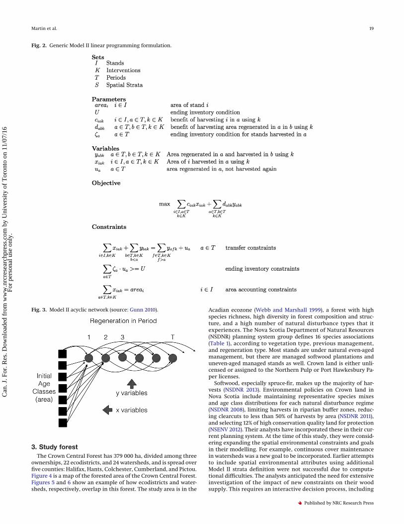
Johnson and Scheurman (1977) were the first to publish a tech-nical description of LP forest management models and classifiedthe two main variants as Model I and Model II. In practice, Model Ihas been employed by Curtis (1962), MaxMillion (Ware and Clutter1971), Timber RAM (Navon 1971), JLP (Lappi 1992), Nelson et al.(1991), and more recently, in Heureka (Wikström et al. 2011) and inthe updated version of JLP, called J (Lappi and Lempinen 2014).Model II is the basis of the Woodstock™ planning system (Feunekesand Cogswell 2000) and also the USDA Forest Service models ForPlan(Kent et al. 1991) and Spectrum (Greer and Meneghin 2002). Thesesystems are used widely and with considerable success in support-ing sustainable harvest management. Although either modelcan be used to support strategic planning, there are significantstructural differences that impact their capabilities and solvabil-ity in particular circumstances. Figures 1 and 2 show equations forgeneric models I and II, respectively.

We refer to Model I as “spatial” because decisions are applied tospecific locations in the forest, called stands. Stands are identicalin all attributes that are tracked and used in the model. Theseattributes describe the stand forest type at varying levels of detail,its forest growth potential, and age. Nonbiological attributes suchas distance to riparian features, location in watershed, ecodistrict,ownership, and so forth are also identical in a stand. Stands do notchange location over time, although their forest attributes changethrough growth and silvicultural interventions. Stands are com-monly assumed to be contiguous, although this has no bearing onthe nature and performance of Model I. In fact, in our study, weincluded stands composed of nonadjacent polygons when allother relevant attributes are identical.

In Model II, forest stands are aggregated into strata that aredefined in a similar way but usually without any knowledge ofspatial location of individual stands or other physical attributessuch as area or edge length. What is “known” in Model II is thenumber of hectares in each stratum at the beginning of each

Martin et al. 17

Published by NRC Research Press

Can

. J. F

or. R

es. D

ownl

oade

d fr

om w

ww

.nrc

rese

arch

pres

s.co

m b

y U

nive

rsity

of

Tor

onto

on

11/0

7/16

For

pers

onal

use

onl

y.

planning period. Hectares in each stratum are transitioned to newstrata at the end of each planning period as the forest is changedthrough growth, aging, and silviculture. Model II is often referredto as an aspatial model due to this lack of spatial definition, al-though spatial attributes can be incorporated by adding morestrata to define location.

Both models incorporate a predefined set of silvicultural inter-ventions or actions such as clear-cut harvest, precommercial thin-ning, commercial thinning, planting, and shelterwood harvest. InModel I, prescriptions are composed of a series of interventionsoccurring over the span of the planning horizon, and each stand isassigned one prescription. For example, a prescription may be to“Clear-cut at age 60, regenerate naturally, and clear-cut again atage 60”. Model II applies actions at different levels (area) in eachstratum and in each planning period. In Model II, prescriptionsare created dynamically in the model and are controlled only byeligibility constraints on actions. In Model I, all prescriptions arepre-specified.

These differences are of course reflected in the decision vari-ables (Figs. 1 and 2), as well as some of the constraints. In Model I,the variables are denoted as xij, i.e., the number of hectares ofstand i to manage under prescription j. In Model II, the variablesare denoted as yabks, i.e., the number of hectares from strata sregenerated in period a and treated in period b using intervention k.The number of decision variables in Model I is the number of validstand–prescription pairs, which is usually much less than thenumber of stands times the number of prescriptions. In Model II, thenumber of variables increases with the number of strata, planningperiods, and interventions that are included.

To manage transitions of forest at the end of each period inModel II, it is necessary to update the new area in each strata. Thisis done with constraints that transfer hectares from one stratumto another, depending on their treatment in the current period.This makes for fewer decision variables, but stand identity is lostwhen actions are applied. The decision variables in Model II can bevisualized as the arcs in an acyclic network (Fig. 3), where actionsapplied in one planning period determine a transition of area to

different strata in the subsequent period. It turns out that theconstraints required to manage this network can impose a signif-icant computational burden. Unfortunately for Model II users,when multiple and overlapping spatial goals are included, morestrata and larger constraint networks are required. It has beenobserved by Model II users that models can “blow up” when toomany strata are included, often as a result of attempts to includemultiple levels of spatial resolution. Each additional spatial attri-bute with, say, n possibilities, increases the number of strata by n.Then, an additional arc is required for each of these n new strata,for each eligible action on each stratum, and for each period andpossible transition. This is what leads to substantial increases inmodel size, which, in turn, leads to unacceptably long solutiontimes.

An important distinction between the models is the nature oftheir prescription sets. As mentioned earlier, Model I prescrip-tions are predefined by the user and consist of a sequence ofactions. These always include a “do nothing” action, and hence,one could visualize a prescription as a vector of actions, one foreach planning period. The type and timing of silvicultural actionsmust be suitable for the stand type and consistent with forestrybest management practices. Thus, there will be a practical limit tothe number of prescriptions that should be generated. However,care must be taken not to limit the model by too restrictive aprescription set. Thus, on one hand, a disadvantage of Model I isthat it is up to the user to determine the prescriptions it attemptsto model (Davis et al. 2001) and generating a comprehensive pre-scription set can be arduous. On the other hand, explicitly speci-fying prescriptions is an advantage in that the process ofgenerating prescriptions can be controlled to produce only thosethat satisfy certain forestry goals, including local sustainability.This is not necessarily the case with Model II.

Model II creates prescriptions dynamically by applying actionsin each period. If insufficient care is given to restricting eligibilityof these actions, illogical sequences may be created. The user onlyhas to define individual silvicultural interventions and the stratafor which they are eligible and is not forced to think about howthey might be combined into prescriptions. Thus, Model II solu-tions can contain prescriptions such as “Shelterwood in periods 1and 3, precommercial thin in period 5, commercial thin in period 9,clear-cut in period 12, and clear-cut in period 20”. Each individualintervention may be reasonable, but the sequence lacks credibil-ity with regard to good forestry practices. Furthermore, becausestand identity is not maintained in Model II, it is impossible todetermine the prescription the model assigns to each stand, so itis not always possible for the user to know the percentage of theirsolution that was developed from these undesirable sequences.

Why do such inconsistencies arise in the optimal solution? Thenature of optimization models is to aggressively seek opportuni-ties to improve the objective function. Forest strategic planningmodels usually have an objective to maximize harvest value and(or) volume. The LP solver will then compose any allowablesequence that increases the harvest. Because results of thesesequences are not necessarily assigned to the same stand, thesebenefits (i.e., harvest volumes) may in fact be impossible toachieve. Thus, we can know that some of the objective function isdue to these computer-generated series of actions that do notrepresent good forestry practices, but it is near impossible to re-move them all from the system.

Finally, Model I solutions are easier to interpret because allow-able prescriptions are predefined and applied to particular stands.With Model II, it may be quite difficult to determine the forestrydecisions that create a given solution, and as there is no standresolution, it is impossible to determine the proposed sequence ofinterventions to verify that they make valid forestry sense.

Fig. 1. Generic Model I linear programming formulation.

18 Can. J. For. Res. Vol. 00, 0000

Published by NRC Research Press

Can

. J. F

or. R

es. D

ownl

oade

d fr

om w

ww

.nrc

rese

arch

pres

s.co

m b

y U

nive

rsity

of

Tor

onto

on

11/0

7/16

For

pers

onal

use

onl

y.

3. Study forestThe Crown Central Forest has 379 000 ha, divided among three

ownerships, 22 ecodistricts, and 24 watersheds, and is spread overfive counties: Halifax, Hants, Colchester, Cumberland, and Pictou.Figure 4 is a map of the forested area of the Crown Central Forest.Figures 5 and 6 show an example of how ecodistricts and water-sheds, respectively, overlap in this forest. The study area is in the

Acadian ecozone (Webb and Marshall 1999), a forest with highspecies richness, high diversity in forest composition and struc-ture, and a high number of natural disturbance types that itexperiences. The Nova Scotia Department of Natural Resources(NSDNR) planning system group defines 16 species associations(Table 1), according to vegetation type, previous management,and regeneration type. Most stands are under natural even-agedmanagement, but there are managed softwood plantations anduneven-aged managed stands as well. Crown land is either unli-censed or assigned to the Northern Pulp or Port Hawkesbury Pa-per licenses.

Softwood, especially spruce-fir, makes up the majority of har-vests (NSDNR 2013). Environmental policies on Crown land inNova Scotia include maintaining representative species mixesand age class distributions for each natural disturbance regime(NSDNR 2008), limiting harvests in riparian buffer zones, reduc-ing clearcuts to less than 50% of harvests by area (NSDNR 2011),and selecting 12% of high conservation quality land for protection(NSENV 2012). Their analysts have incorporated these in their cur-rent planning system. At the time of this study, they were consid-ering expanding the spatial environmental constraints and goalsin their modelling. For example, continuous cover maintenancein watersheds was a new goal to be incorporated. Earlier attemptsto include spatial environmental attributes using additionalModel II strata definition were not successful due to computa-tional difficulties. The analysts anticipated the need for extensiveinvestigation of the impact of new constraints on their woodsupply. This requires an interactive decision process, including

Fig. 2. Generic Model II linear programming formulation.

Fig. 3. Model II acyclic network (source: Gunn 2010).

Martin et al. 19

Published by NRC Research Press

Can

. J. F

or. R

es. D

ownl

oade

d fr

om w

ww

.nrc

rese

arch

pres

s.co

m b

y U

nive

rsity

of

Tor

onto

on

11/0

7/16

For

pers

onal

use

onl

y.

sensitivity analysis of the importance of stochastic factors suchas stand development uncertainties. Hence, they have a need for asystem that could produce new solutions quickly and generatemany instances for analysis as scenarios are proposed and evalu-ated.

4. Study strategic planning modelsTwo strategic planning LP models were used to investigate the

capabilities of Model I and Model II. Both models needed to incor-porate NSDNR goals for ecosystem-based landscape management.

We used their current system, Woodstock™, which incorporates aModel II type of optimization. We formulated a spatial Model I anddeveloped a prescription system that matched the current aspa-tial model as closely as possible. Our Model I follows the structureof the theoretical, comprehensive Model I formulation presentedin Gunn (2010).

Figure 7 delineates the sets, parameters, and variables used forModel I. Note that sets are used to group stands by ownership,natural disturbance regime, ecodistrict, and watershed. Coeffi-cients are used to calculate important features of a solution. For

Fig. 4. The Crown Central Forest, Nova Scotia, Canada. Figure is provided in colour online.

Fig. 5. Section of central Nova Scotia showing ecodistricts (source:NSDNR 2007).

Fig. 6. Section of central Nova Scotia showing watersheds (source:NSENV 2011).

20 Can. J. For. Res. Vol. 00, 0000

Published by NRC Research Press

Can

. J. F

or. R

es. D

ownl

oade

d fr

om w

ww

.nrc

rese

arch

pres

s.co

m b

y U

nive

rsity

of

Tor

onto

on

11/0

7/16

For

pers

onal

use

onl

y.

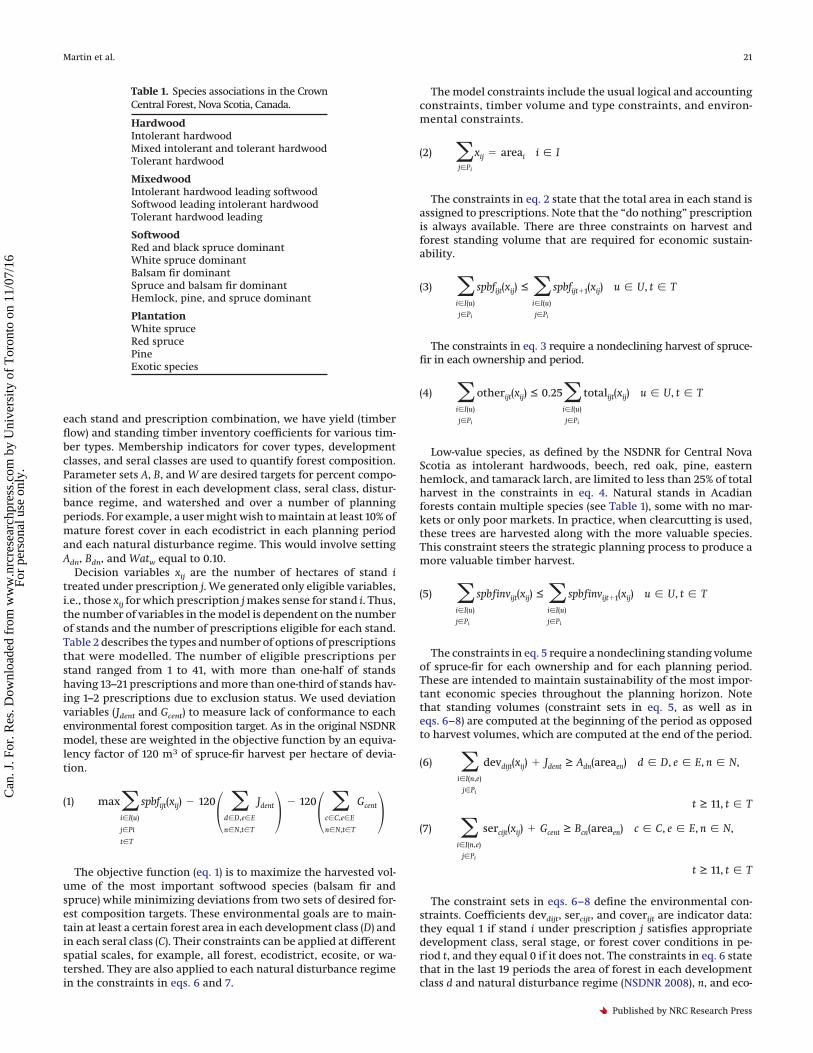
each stand and prescription combination, we have yield (timberflow) and standing timber inventory coefficients for various tim-ber types. Membership indicators for cover types, developmentclasses, and seral classes are used to quantify forest composition.Parameter sets A, B, and W are desired targets for percent compo-sition of the forest in each development class, seral class, distur-bance regime, and watershed and over a number of planningperiods. For example, a user might wish to maintain at least 10% ofmature forest cover in each ecodistrict in each planning periodand each natural disturbance regime. This would involve settingAdn, Bdn, and Watw equal to 0.10.

Decision variables xij are the number of hectares of stand itreated under prescription j. We generated only eligible variables,i.e., those xij for which prescription j makes sense for stand i. Thus,the number of variables in the model is dependent on the numberof stands and the number of prescriptions eligible for each stand.Table 2 describes the types and number of options of prescriptionsthat were modelled. The number of eligible prescriptions perstand ranged from 1 to 41, with more than one-half of standshaving 13–21 prescriptions and more than one-third of stands hav-ing 1–2 prescriptions due to exclusion status. We used deviationvariables (Jdent and Gcent) to measure lack of conformance to eachenvironmental forest composition target. As in the original NSDNRmodel, these are weighted in the objective function by an equiva-lency factor of 120 m3 of spruce-fir harvest per hectare of devia-tion.

(1) max�i�I(u)

j�Pi

t�T

spbfijt(xij) � 120� �d�D,e�E

n�N,t�T

Jdent� � 120� �c�C,e�E

n�N,t�T

Gcent�The objective function (eq. 1) is to maximize the harvested vol-

ume of the most important softwood species (balsam fir andspruce) while minimizing deviations from two sets of desired for-est composition targets. These environmental goals are to main-tain at least a certain forest area in each development class (D) andin each seral class (C). Their constraints can be applied at differentspatial scales, for example, all forest, ecodistrict, ecosite, or wa-tershed. They are also applied to each natural disturbance regimein the constraints in eqs. 6 and 7.

The model constraints include the usual logical and accountingconstraints, timber volume and type constraints, and environ-mental constraints.

(2) �j�Pi

xij � areai i � I

The constraints in eq. 2 state that the total area in each stand isassigned to prescriptions. Note that the “do nothing” prescriptionis always available. There are three constraints on harvest andforest standing volume that are required for economic sustain-ability.

(3) �i�I(u)

j�Pi

spbfijt(xij) ≤ �i�I(u)

j�Pi

spbfijt�1(xij) u � U, t � T

The constraints in eq. 3 require a nondeclining harvest of spruce-fir in each ownership and period.

(4) �i�I(u)

j�Pi

otherijt(xij) ≤ 0.25�i�I(u)

j�Pi

totalijt(xij) u � U, t � T

Low-value species, as defined by the NSDNR for Central NovaScotia as intolerant hardwoods, beech, red oak, pine, easternhemlock, and tamarack larch, are limited to less than 25% of totalharvest in the constraints in eq. 4. Natural stands in Acadianforests contain multiple species (see Table 1), some with no mar-kets or only poor markets. In practice, when clearcutting is used,these trees are harvested along with the more valuable species.This constraint steers the strategic planning process to produce amore valuable timber harvest.

(5) �i�I(u)

j�Pi

spbfinvijt(xij) ≤ �i�I(u)

j�Pi

spbfinvijt�1(xij) u � U, t � T

The constraints in eq. 5 require a nondeclining standing volumeof spruce-fir for each ownership and for each planning period.These are intended to maintain sustainability of the most impor-tant economic species throughout the planning horizon. Notethat standing volumes (constraint sets in eq. 5, as well as ineqs. 6–8) are computed at the beginning of the period as opposedto harvest volumes, which are computed at the end of the period.

(6) �i�I(n,e)

j�Pi

devdijt(xij) � Jdent ≥ Adn(areaen) d � D, e � E, n � N,

t ≥ 11, t � T

(7) �i�I(n,e)

j�Pi

sercijt(xij) � Gcent ≥ Bcn(areaen) c � C, e � E, n � N,

t ≥ 11, t � T

The constraint sets in eqs. 6–8 define the environmental con-straints. Coefficients devdijt, sercijt, and coverijt are indicator data:they equal 1 if stand i under prescription j satisfies appropriatedevelopment class, seral stage, or forest cover conditions in pe-riod t, and they equal 0 if it does not. The constraints in eq. 6 statethat in the last 19 periods the area of forest in each developmentclass d and natural disturbance regime (NSDNR 2008), n, and eco-

Table 1. Species associations in the CrownCentral Forest, Nova Scotia, Canada.

HardwoodIntolerant hardwoodMixed intolerant and tolerant hardwoodTolerant hardwood

MixedwoodIntolerant hardwood leading softwoodSoftwood leading intolerant hardwoodTolerant hardwood leading

SoftwoodRed and black spruce dominantWhite spruce dominantBalsam fir dominantSpruce and balsam fir dominantHemlock, pine, and spruce dominant

PlantationWhite spruceRed sprucePineExotic species

Martin et al. 21

Published by NRC Research Press

Can

. J. F

or. R

es. D

ownl

oade

d fr

om w

ww

.nrc

rese

arch

pres

s.co

m b

y U

nive

rsity

of

Tor

onto

on

11/0

7/16

For

pers

onal

use

onl

y.

district, e, should be Adn percentage of total area in that ecodistrictand natural disturbance regime. Deviations from these goals arerecorded in the Jdent variables, which are penalized in the objectivefunction at 120 m3·ha–1. The constraints in eq. 7 are similar tothose in eq. 6 but applied to seral stage (Stewart and Neilly 2008)instead of development class. The Gcent variables record deviationsfrom these targets and are penalized in the same way as the Jdentvariables. As is common in forest strategic planning, dependingon the initial structure of the forest, the model may not be feasiblein every period. Penalty weights and A and B parameter valueswere provided by the NSDNR. In this instance, the initial state ofthe forest was vastly different from these targets. Hence, the en-vironmental constraints were applied after 11 planning periods,allowing a “warm-up” time so that the forest can be managed toattain this structure over time.

(8) �i�I(w)

j�Pi

coverijt(xij) ≥ Watw(areaw) w � W, t ≥ 5, t � T

The constraints in eq. 8 are the sole case of an element beingintroduced to this study that was not in the original NSDNRWoodstock™ model. They state that, in the last 25 periods, at leastWatw percent of the forest in each watershed, w, must qualify assuitable watershed forest cover, i.e., not be in an establishmentdevelopment class.

The Model II model, built using the Woodstock™ system, isanalogously defined; copies of the files that describe its structurecan be found in Martin (2013). Figure 2 shows a generic Model IIformulation. Model II decision variables xiak represent the area ofstand i harvested in period a using intervention k. Variables yabk

represent the area regenerated in period a and then harvestedagain in period b, using intervention k. Parameters ciak and dabk

represent the benefit accruing from harvesting stand i in period ausing intervention k and harvesting a hectare in period a thenagain in period b using intervention k, respectively. Network con-straints in eq. 2 ensure the area harvested in period b is regener-ated and harvested again in period f or allowed to remainunharvested and pass into ua. The ending inventory constraints ineq. 3 ensure a certain harvestable area remains at the end of theplanning horizon. Area accounting constraints in eq. 4 ensure the

Fig. 7. Model I linear programming formulation: sets, parameters, and variables.

Table 2. Phase 2 Model I prescriptions.

No. of options

Prescription type Age (years) Phase 1 Phase 2

Clear-cut 55+ 80 80Shelterwood 60 and 70 1 18Thinning 15–95 45 96Selection 80 6 11Buffer harvest 60 1 1

22 Can. J. For. Res. Vol. 00, 0000

Published by NRC Research Press

Can

. J. F

or. R

es. D

ownl

oade

d fr

om w

ww

.nrc

rese

arch

pres

s.co

m b

y U

nive

rsity

of

Tor

onto

on

11/0

7/16

For

pers

onal

use

onl

y.

area harvested from each stand is equal to the area covered by thatstand.

Identical yield data yijkt was used in both models. It came fromthe NS Growth and Yield model for even-aged stands and frompermanent sample plot (PSP) data for uneven aged stands (O’Keefeand McGrath 2006). The same silvicultural interventions were de-fined in both models: clear-cut, pre-commercial thinning, com-mercial thinning, shelterwood harvest, selection harvest, andbuffer harvest.

For all comparisons, 68 346 stands were modelled. These werederived from the NSDNR data of 176 480 forested contiguousstands by aggregating those that shared the same ecodistrict, nat-ural disturbance regime, watershed, county, species association,forest state, stocking level, site class, riparian status, exclusionstatus, ownership, and age.

5. Study methodsWe defined four scenarios (Table 3) that are increased in spatial

resolution by successively adding ownership, ecodistrict, and wa-tershed constraints. We solved models I and II under each sce-nario twice. In phase 1, a restricted prescription set (Table 2) wasused to calibrate the models and to investigate relative perfor-mance on a test-sized problem. The second phase expanded theprescription timing options so that Model I would be equal incomplexity to the models used in practice by NSDNR. Phase 1 had144 prescription types and phase 2 had 206 prescription types. Thestudy forest stands and data were used identically in all cases.

For phase 1, we needed to modify the NSDNR Woodstock™model to ensure that its prescription set was comparable withthat of Model I (see Table 2). We severely restricted eligibility ofthe Woodstock™ system’s actions, limiting second and thirdtreatments depending on the initial intervention. For example,area that was clear-cut as a first intervention could only be clear-cut at a specified age for the second and third interventions orarea that was commercially thinned as a first intervention wouldreceive a commercial thin again after its initial final-felling. Withthe restricted Model II, interventions could not be mixed freely,and we were able to create a problem that was nearly identical toour Model I instance. In addition to facilitating calibration, phase 1provided data for a small implementation that could be computedquickly and produced preliminary results on performance andfeasibility of the models.

In the second phase, restrictions were removed from Model II.Commercial thinning, shelterwood, selection, and clear-cut inter-ventions could be combined within operability limits. Additionaltiming options were added to the Model I prescriptions so that thefirst entry did not determine future entries and hence approxi-mated Model II’s expanded prescription set. Phase 2 models rep-resented the current and anticipated level of use by NSDNR andwere verified using their historical data. This phase allowed usto gain insight into potential for implementing further spatialdetail.

Due to licensing restrictions and for efficiency, Model I andModel II models were run on different computers. Model I was runon 64 bit Windows 7 with 8 Gb of RAM and a 2.53 Ghz processor,and Model II was run on 64 bit Windows 7 with 8 Gb of RAM anda slightly faster 3.00 Ghz processor. Both computers were net-worked, and thus a fully controlled computational environment

was not possible. Nevertheless, every attempt was made to keepthe model runs as undisturbed as possible. Model I models weregenerated using AMPL (Fourer et al. 1993), and Model II modelswere generated within Woodstock™.

6. ResultsAll problem instances were solved to optimality using the con-

current optimizer in Gurobi 5.1.1 (Gurobi Optimization Inc. 2013).Tables 4 and 5 show dimensions of Model I and Model II for each

scenario in phase 1 and phase 2, respectively. For Model I, thenumber of constraints (rows) and matrix density (nonzeroes)change very little (6% and 0.02%) as additional spatial consider-ations are added. For Model II, the constraints increase from260 296 to 722 002 in phase 1 and from 322 852 to 1 156 015 inphase 2, which is a total increase of 358%. The number of decisionvariables in Model II increases from 787 506 to 1 823 163 in phase 1and from 821 549 to 2 900 105 in phase 2, which is a total increaseof 353%. Model II matrix nonzeroes exhibits a similar, yet moredramatic pattern. It moves from 1 700 820 to 100 002 631 in phase 1and from 1 646 491 to 120 417 153 in phase 2, which is a totalincrease of 7314%.

Model I has identical variables (columns) across scenarios. Wecalculated all harvest flows and environmental values indicatorseven if they were not constrained or penalized. This increased thesize of the initial constraint set, and hence, the percent increase inmatrix density across scenarios is smaller than it could be.

Tables 6 and 7 summarize solution CPU time and quality forphase 1 and phase 2 scenarios, respectively. Figures 8 and 9 pres-ent the results graphically. There was little difference in modelpreparation times: all were in the order of 20 min. Hence, weomitted the fixed cost of pre-processing and model building inthese results.

Computationally, Model I significantly outperformed Model IIin scenarios 3 and 4 (Tables 6 and 7). In both phases, the CPU timefor Model II increases dramatically as constraints are added to themodel, whereas for Model I, the CPU time increases are small. Thisis further illustrated in Figs. 8 and 9 that show the relatively largeincrease in solution time for Model II in both phases as spatialresolution increases. Computational results for scenarios 1 and 2are anomolous: Model II outperforms Model I in these cases.

In phase 1, Model I attained lesser objective values than Model IIat 98.43%, 97.91%, 95.46%, and 95.43% of Model II objectives forscenarios 1, 2, 3, and 4, respectively. In phase 2, however, Model Iand Model II objective functions were nearly identical.

Recall that the objective function (eq. 1 is a sum of harvestvolumes and penalties for not meeting environmental targets.Solution quality in this paper refers only to the numeric value ofthe mathematical objective function, which can be composed ofany combination of harvest and penalties. As an example, Fig. 8shows the penalties per period for Model I, phase 2, scenario 3.The total of these penalties is 12 267 ha, representing 1 472 040 m3

weighted at 120 m3·ha–1. These account for approximately 3.5% ofthe total objective function. Penalties in the equivalent Model IIwere almost exactly 5000 ha, corresponding to 600 000 m3.

7. DiscussionThe strategic planning study we undertook is extensive both in

scope and in problem size. It includes several important elementsof sustainable spatial forest management, namely economic re-turn from harvesting and landscape-level structure by ecodistrict,natural disturbance regime, ownership, and watershed. The studywas executed on a large forest of 379 000 ha divided betweenabout 68 000 stands and includes a comprehensive set of 206 pre-scriptions (Table 3).

The study results confirm our hypothesis that Model I would becomputationally preferable to Model II. Although both modelscan express spatial constraints and goals, Model I is more robust

Table 3. Scenario definitions.

Scenario Description

Constraints

3 4 5 6 7 8

1 Base No No No No No No2 Timber constraints Yes Yes Yes No No No3 Ecodistrict constraints Yes Yes Yes Yes Yes No4 Watershed constraints Yes Yes Yes Yes Yes Yes

Martin et al. 23

Published by NRC Research Press

Can

. J. F

or. R

es. D

ownl

oade

d fr

om w

ww

.nrc

rese

arch

pres

s.co

m b

y U

nive

rsity

of

Tor

onto

on

11/0

7/16

For

pers

onal

use

onl

y.

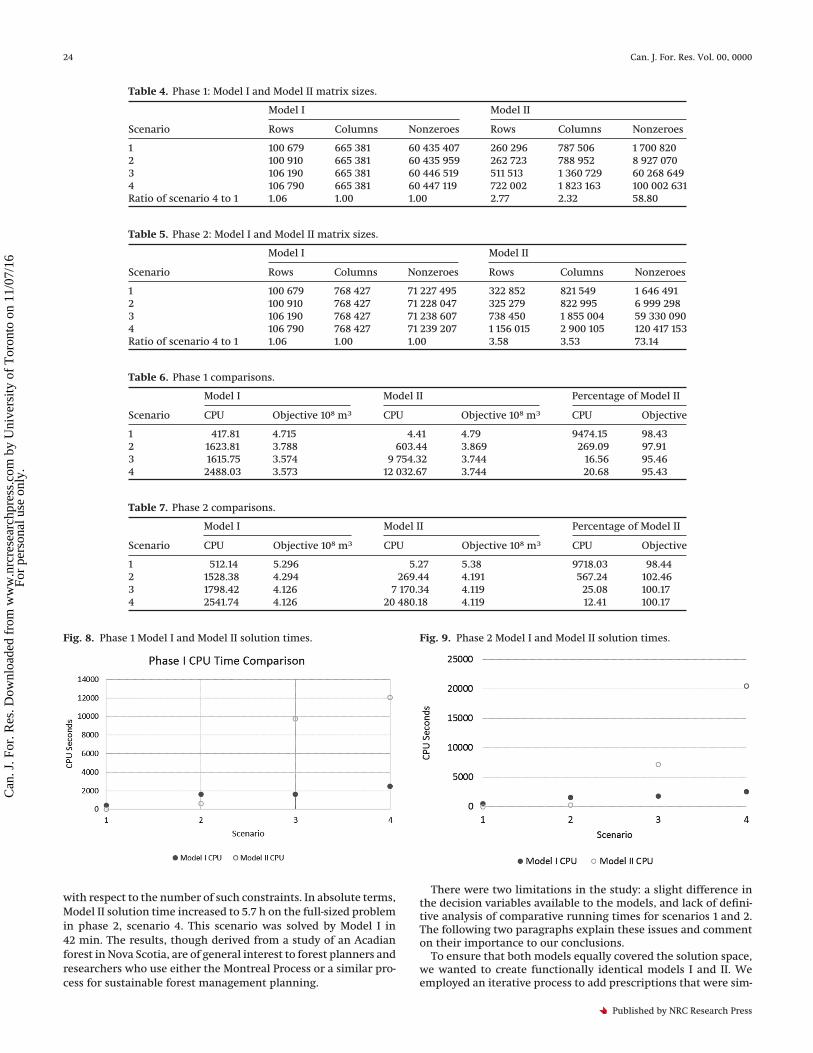
with respect to the number of such constraints. In absolute terms,Model II solution time increased to 5.7 h on the full-sized problemin phase 2, scenario 4. This scenario was solved by Model I in42 min. The results, though derived from a study of an Acadianforest in Nova Scotia, are of general interest to forest planners andresearchers who use either the Montreal Process or a similar pro-cess for sustainable forest management planning.

There were two limitations in the study: a slight difference inthe decision variables available to the models, and lack of defini-tive analysis of comparative running times for scenarios 1 and 2.The following two paragraphs explain these issues and commenton their importance to our conclusions.

To ensure that both models equally covered the solution space,we wanted to create functionally identical models I and II. Weemployed an iterative process to add prescriptions that were sim-

Table 4. Phase 1: Model I and Model II matrix sizes.

Scenario

Model I Model II

Rows Columns Nonzeroes Rows Columns Nonzeroes

1 100 679 665 381 60 435 407 260 296 787 506 1 700 8202 100 910 665 381 60 435 959 262 723 788 952 8 927 0703 106 190 665 381 60 446 519 511 513 1 360 729 60 268 6494 106 790 665 381 60 447 119 722 002 1 823 163 100 002 631Ratio of scenario 4 to 1 1.06 1.00 1.00 2.77 2.32 58.80

Table 5. Phase 2: Model I and Model II matrix sizes.

Scenario

Model I Model II

Rows Columns Nonzeroes Rows Columns Nonzeroes

1 100 679 768 427 71 227 495 322 852 821 549 1 646 4912 100 910 768 427 71 228 047 325 279 822 995 6 999 2983 106 190 768 427 71 238 607 738 450 1 855 004 59 330 0904 106 790 768 427 71 239 207 1 156 015 2 900 105 120 417 153Ratio of scenario 4 to 1 1.06 1.00 1.00 3.58 3.53 73.14

Table 6. Phase 1 comparisons.

Scenario

Model I Model II Percentage of Model II

CPU Objective 108 m3 CPU Objective 108 m3 CPU Objective

1 417.81 4.715 4.41 4.79 9474.15 98.432 1623.81 3.788 603.44 3.869 269.09 97.913 1615.75 3.574 9 754.32 3.744 16.56 95.464 2488.03 3.573 12 032.67 3.744 20.68 95.43

Table 7. Phase 2 comparisons.

Scenario

Model I Model II Percentage of Model II

CPU Objective 108 m3 CPU Objective 108 m3 CPU Objective

1 512.14 5.296 5.27 5.38 9718.03 98.442 1528.38 4.294 269.44 4.191 567.24 102.463 1798.42 4.126 7 170.34 4.119 25.08 100.174 2541.74 4.126 20 480.18 4.119 12.41 100.17

Fig. 8. Phase 1 Model I and Model II solution times. Fig. 9. Phase 2 Model I and Model II solution times.

24 Can. J. For. Res. Vol. 00, 0000

Published by NRC Research Press

Can

. J. F

or. R

es. D

ownl

oade

d fr

om w

ww

.nrc

rese

arch

pres

s.co

m b

y U

nive

rsity

of

Tor

onto

on

11/0

7/16

For

pers

onal

use

onl

y.

ilar to Model II optimal choices until Model I and Model II objec-tive function values were near identical. We were unable toreplicate the full scope of the Model II decision variables. Table 6shows that with phase 1 restricted prescription sets, Model Iachieves about 5% lower objective values than Model II. Thus, ourability to force the Model II system to duplicate a restricted set ofprescriptions in Model I was close but not entirely successful.Objective function values for phase 2 (Table 7) were near identical,within a fraction of 1%. This implies that we were able to betterreplicate Model II decision variables with the expanded Model Iprescription set used in phase 2. This approach does not guaran-tee that all interventions are modelled identically, explaininghow Model I finds slightly higher objective values in phase 2,scenarios 2–4 (Table 7). These small differences do not change ourconclusions about the trends in model size and computationaleffectiveness as spatial constraints are added.

Table 7 shows that with a more realistic prescription set Model Iachieves almost identical objective values as Model II and solvesthese models up to eight times faster. We note the anomaly inrelative computational performance of Model I in scenarios 1 and2. As shown in Tables 6 and 7 and graphically seen in Figs. 8 and 9,in scenarios 1 and 2, Model II actually outperforms Model I. Wesuggest that this may be explained by the fact that the initialModel I matrix is already quite dense. In Table 5, we see that theModel I matrix size increases only marginally from scenario 1 toscenario 4 in both phases. This is partly due to the fact that whendefining the number of stands and prescriptions available to eachstand, most of the matrix is determined at the basecase level.Additionally, all scenario models had the same inventory con-straints and variables. So, for example, all of the scenario 1 modelshad watershed inventory variables. These variables and con-straints only tracked quantities and hence did not constrain thesolution. For this reason, they would have likely been removedduring the Gurobi presolve, potentially skewing Model I solutiontimes to be slightly higher. The effect is not obvious in scenario 3as the performance of Model I overwhelms that of Model II. Inscenario 4, they are formulated equally.

We have stated earlier that it is easier to understand prescription-based solutions and that explicitly defining prescriptions can as-sure users that only best forestry practices are modelled. This isnot the case with Model II, where sequences of actions are lesseasy to control. Model II can create a sequence of treatments thatare less than acceptable. An example of one of these “inconsistentprescriptions” from our case study is as follows: if a stand was14 periods old in period 1, it could receive a shelterwood first entryimmediately, a second entry in period 3, and then be placed on acommercial thinning regime starting in period 16. This odd se-quence of events was produced by a computer “puzzle solver”. It isnot the sort of silviculture that meets good forestry practice stan-dards. And so, subject to the caveat that a comprehensive set ofprescriptions suitable for the landscape is generated, Model I inour opinion is a better choice. Generating a complete set of pre-scriptions is a nontrivial task and does require additional effortrequired by users. Some prescription generation systems exist, forexample, in the Heureka system (Wikström et al. 2011).

Structure of the optimal solution can be quite different giveneven small changes to the linear programming model. In ourmodels, deviation variables are used to ensure feasible solutionsfor the constraints in eqs. 6 and 7. The objective function has twoterms: the sum of harvest volumes and penalties due to noncom-pliance to environmental constraints. In this limited study, Model Itended to produce solutions with higher penalties. For example,violations to the ecosystem constraints for the Model I, phase 2,scenario 3 model (Table 8) sum to 12 267 ha of violation. For allphases and scenarios, penalties were about 2.5 times higher inModel I than in Model II. We did not focus on this aspect ofsolution quality. In practice, users would address this aspect of the

solution by employing additional constraints to limit penalties orto spread penalties over planning periods.

A natural question to ask is “Will Model I continue to performwell on larger forests and with increased complexity in constraintstructure?” The example in this paper, with 68 346 stands andthree spatial constraint sets, exhibited a modest increase in com-putation time with added constraints as exhibited visually inFigs. 8 and 9.

Model I size is directly proportional to the number of validstand–prescription pairs. Therefore, we hypothesize that thistrend of gradual increase in solution time will remain as largerproblem instances (forests) and additional spatial constraints areincluded. However, increased size of problem instance and com-plexity of model may lead to other complications in computingsuch as memory management issues. That said, the problemssolved in this study were done on very modest computers andwithout effort to optimize code and data transfer. The next obvi-ous step is to expand the study to larger forests and to includeother important spatial considerations. One obvious candidate isto include mill demands, prices, and costs of transportation tomills so that profit maximization can be done. These supply chainfactors are enormously important in managing forests sustain-ably. In Martin (2013), other work demonstrates that the inclusionof basic economics, as suggested in Gunn (2010), is entirely feasi-ble within the Model I framework.

This paper should not be viewed as a criticism of the Woodstock™system per se, other than the limitations inherent in its Model IIstructure. We mentioned the system specifically because it is thesoftware the NSDNR uses. Furthermore, we did not have access tosource code and that impacted our ability to identically reproducetheir model in a Model I form. The main point of our paper is theModel I versus Model II modelling framework comparison and notthe environment in which they are implemented.

8. Summary and conclusionsThis paper has shown that Model I is a promising framework in

which to model forest management strategy with spatial con-straints. With respect to computation time, it outperformedModel II conclusively, obtaining comparable optimal solutions inthe order of 10% of Model II’s CPU time while incorporating mul-

Table 8. Per period violationson Model I, phase 2, scenario 3model.

Period Violation (ha)

11 1586.512 954.413 671.614 372.315 314.916 82.417 60.118 22.719 4.420 4.621 38.022 5.723 20.624 59.925 84.826 169.927 356.928 999.629 2417.930 4039.9

Note: The ecosystem constraintsthese violations are associated withare not applied prior to period 11.

Martin et al. 25

Published by NRC Research Press

Can

. J. F

or. R

es. D

ownl

oade

d fr

om w

ww

.nrc

rese

arch

pres

s.co

m b

y U

nive

rsity

of

Tor

onto

on

11/0

7/16

For

pers

onal

use

onl

y.

tiple overlapping spatial goals, including environmental objec-tives. Model II’s CPU time increased, as spatial constraints wereadded, to unacceptable levels. This empirical evidence of relativemodel performance and model matrix changes is supported bythe technical exposition of the difference in model structure.Hence, we are comfortable in stating that these results are gener-alizable, i.e., not due to case-specific factors.

This is to our knowledge the first published comparison ofthese models on modern spatial strategic forest managementplanning problems, and our results provide new and importantguidance to users and researchers about expected relative perfor-mance of these two formulations. Model II may outperform Model Iin some situations, particularly when there are no spatial con-straints. However, we have refuted the common expectation thatModel II reduces the size and difficulty of linear programming har-vest scheduling models relative to Model I in all situations.

Modern forest management must address the cumulative ef-fects of silvicultural interventions over large landscape mosaicsand long timeframes. Increasingly, stakeholders have collabo-rated and developed international standards for sustainable for-est management and conservation. The Montreal Process criteriaand indicators (Montreal Process 1998) for sustainable forest man-agement framework is a globally adopted strategy. Credible forestmanagement processes must incorporate these “essential compo-nents of strategic forest management” (Montreal Process 1998)in locally meaningful ways. This, in most if not all jurisdictions,means that the forest must be managed and assessed by its cur-rent and future condition at several scales: in watersheds, ecodis-tricts, riparian zones, and ownership at a minimum. Optimizationmodels like Model I that support this spatial resolution can moreaccurately assess and compare proposed policies and strategies,because important spatially referenced ecosystem-based goalsand constraints can be explicitly included. Spatial considerationshave seldom been incorporated directly in strategic planningmodels. They may be dealt with exogenously, for example, bydelineating habitat and protected areas prior to optimization(Nalli et al. 1996; Næsset 1997). Model I systems such as Heureka(Wikström et al. 2011) and Simo (Rasinmäki et al. 2009) have beenused in Europe, but the predominant LP form for strategic plan-ning has been Model II.

Strategic planning as the first phase in a HFM managementprocess is commonly used to determine a first estimate of sustain-able cutting levels or annual allowable cut. This aspatial annualallowable cut is input to a subsequent tactical planning processthat assesses spatial feasibility over a shorter planning horizon asan annual allowable cut target. Increased spatial resolution in thestrategic planning model will improve this estimate, strengthen-ing the linkage between strategic and tactical planning phases ofHFM.

In addition to the inherent likelihood of suboptimal solutionsfrom systems of disaggregated models, there remains uncertaintyabout long-term ecosystem sustainability when spatial consider-ations are assessed on short time horizons and, sometimes, on asubset of the forest. Other concerns about the divergence betweenplanned and implemented forest operations have been noted.Spatial strategic planning models can reduce the gap betweenstrategic planning model outputs and tactical or implementedplans and, hence, contribute to improving HFM processes. Paradiset al. (2013) noted that adding increased detail in forest productdemands in strategic-level models increased coherence betweenlong- and short-term harvest planning solutions significantly. Inthe same way, increasing spatial detail in strategic planning mod-els reduces the gap between strategic and tactical managementsolutions by better forecasting timber harvests that depend onlocation relative to demand points, ecosystems, watersheds, andcommunities.

This work has shown that a Model I framework is a more suit-able modelling framework for representing spatial strategic forest

management than the more commonly used Model II. Futurework will investigate performance on larger forests and determin-ing best structures and modelling for larger problem instances.Additional spatial considerations such as supply chain modellingwill also be investigated.

AcknowledgementsWe acknowledge the Nova Scotia Department of Natural Re-

sources (NSDNR) for their indispensable support for this research.This case study was made possible through collaboration with theNSDNR; they provided the stand inventory, yield data, a copy oftheir Woodstock™ model, and numerous discussions duringmodel development. It remains that all analysis and conclusionsin this work are the sole responsibility of the authors. Funding forthis project was provided by the National Sciences and Engineer-ing Research Council, The VCO network, Dalhousie University,and the University of New Brunswick.

ReferencesBitran, G.R., and Hax, A.C. 1977. On the design of hierarchical production plan-

ning systems. Decision Sci. 8(1): 28–55. doi:10.1111/j.1540-5915.1977.tb01066.x.CCFM. 2003. Canadian Council of Forest Ministers: Defining sustainable man-

agement in Canada [online]. Available from http://www.ccfm.org/pdf/CI_booklet_e.pdf.

Curtis, F.H. 1962. Linear programming the management of a forest property.J. For. 60(9): 611–616.

Davis, L.S., Johnson, K.N., Bettinger, P.S., and Howard, T.E. 2001. Forest manage-ment. 4th ed. McGraw-Hill, New York.

Feunekes, U., and Cogswell, A. 2000. A hierarchical approach to spatial forestplanning. USDA Forest Service, General Technical Report NC 7-13.

Fourer, R., Gay, D.M., and Kernighan, B.W. 1993. AMPL: a modeling language formathematical programming. Vol. 119. Boyd & Fraser, San Francisco.

Greer, K., and Meneghin, B. 2002. Spectrum: an analytical tool for buildingnatural resource management models. Available from http://www.ncrs.fs.fed.us/pubs/gtr/other/gtr-nc205/pdffiles/p53.pdf.

Gunn, E. 2010. Some perspectives on strategic forest management models andthe forest products supply chain. INFOR, 47(3): 261–272. doi:10.3138/infor.47.3.261.

Gurobi Optimization Inc. 2013. Gurobi optimizer reference manual [online].Available from http://www.gurobi.com.

Gustafson, E.J., Roberts, L.J., and Leefers, L.A. 2006. Linking linear programmingand spatial simulation models to predict landscape effects of forest manage-ment alternatives. J. Environ. Manage. 81(4): 339–350. doi:10.1016/j.jenvman.2005.11.009. PMID:16549235.

Johnson, K.N., and Scheurman, H.L. 1977. Techniques for prescribing optimaltimber harvest and investment under different objectives. Discussion andsynthesis. Forest Sci. 18: 1–30.

Kent, B., Bare, B.B., Field, R.C., and Bradley, G.A. 1991. Natural resource landmanagement planning using large-scale linear programs: the USDA forestservice experience with forplan. Oper. Res. 39(1): 13–27. doi:10.1287/opre.39.1.13.

Lappi, J. 1992. JLP-a linear programming package for management planning.Finnish Forest Research Institute, Helsinki.

Lappi, J., and Lempinen, R. 2014. A linear programming algorithm and softwarefor forest-level planning problems including factories. Scand. J. Forest Res.29(Suppl. 1): 178–184. doi:10.1080/02827581.2014.886714.

Martell, D.L., Gunn, E.A., and Weintraub, A. 1998. Forest management chal-lenges for operational researchers. Eur. J. Oper. Res. 104(1): 1–17. doi:10.1016/S0377-2217(97)00329-9.

Martin, A.B. 2013. A linear programming framework for models of forest man-agement strategy. Master’s thesis. Available from https://dalspace.library.dal.ca/handle/10222/37840.

McDill, M.E., Tóth, S.F., St. John, R., Braze, J., and Rebain, S.A. 2016. ComparingModel I and Model II formulations of spatially explicit harvest schedulingmodels with maximum area restrictions. Forest Sci. 62(1): 28–37. doi:10.5849/forsci.14-179.

Montreal Process. 1998. The Montreal process [online]. Available from http://www.mpci.org/whatis/criteria.html.

Næsset, E. 1997. A spatial decision support system for long-term forest manage-ment planning by means of linear programming and a geographical informa-tion system. Scand. J. Forest Res. 12(1): 77–88. doi:10.1080/02827589709355387.

Nalli, A., Nuutinen, T., and Päivinen, R. 1996. Site-specific constraints in inte-grated forest planning. Scand. J. Forest Res. 11(1–4): 85–96. doi:10.1080/02827589609382915.

Navon, D.I. 1971. Timber RAM: a long-range planning method for commercialtimber lands under multiple-use management. USDA Forest Service, PacificSouthwest Forest and Range Experiment Station, Research Paper PSW-RP-70.

Nelson, J. 2003. Forest planning studio (FPS): ATLAS program reference manualversion 6. Faculty of Forestry, University of British Columbia, Vancouver, B.C.

26 Can. J. For. Res. Vol. 00, 0000

Published by NRC Research Press

Can

. J. F

or. R

es. D

ownl

oade

d fr

om w

ww

.nrc

rese

arch

pres

s.co

m b

y U

nive

rsity

of

Tor

onto

on

11/0

7/16

For

pers

onal

use

onl

y.

Nelson, J., Brodie, J.D., and Sessions, J. 1991. Integrating short-term, area-basedlogging plans with long-term harvest schedules. Forest Sci. 37(1): 101–122.

NSDNR. 2007. Nova Scotia Department of Natural Resources. Ecodistricts ofNova Scotia. Available from http://www.gov.ns.ca/natr/forestry/ecological/pdf/ELC_Map.pdf.

NSDNR. 2008. Nova Scotia Department of Natural Resources. Mapping NovaScotia’s natural disturbance regimes. Available from http://novascotia.ca/natr/library/forestry/reports/NDRreport3.pdf.

NSDNR. 2011. The path we share: a natural resource strategy for Nova Scotia2011–2020 [online]. Nova Scotia Department of Natural Resources. Availablefrom http://novascotia.ca/natr/strategy/pdf/Strategy_Strategy.pdf.

NSDNR. 2013. Nova Scotia Department of Natural Resources. Registry of buyersof primary forest products report for 2013–2014. Available from http://www.gov.ns.ca/natr/forestry/registry/annual/2013/2012AnnualReport.pdf.

NSENV. 2011. Nova Scotia Environment. Primary watersheds of Nova Scotia.Available from http://www.gov.ns.ca/nse/water.strategy/docs/WaterStrategy_NSWatershedMap.pdf.

NSENV. 2012. Nova Scotia Environment. Environmental goals and sustainableprosperity act: progress report. Available from http://gov.ns.ca/nse/egspa/docs/EGSPA.2012.Annual.Report.pdf.

O’Keefe, R., and McGrath, T. 2006. Nova Scotia hardwood growth and yieldmodel. Available from http://novascotia.ca/natr/library/forestry/reports/REPORT78.PDF.

Paradis, G., LeBel, L., D’Amours, S., and Bouchard, M. 2013. On the risk of sys-tematic drift under incoherent hierarchical forest management planning.Can. J. For. Res. 43(5): 480–492. doi:10.1139/cjfr-2012-0334.

Pretzsch, H., Grote, R., Reineking, B., Rötzer, T., and Seifert, S. 2008. Models forforest ecosystem management: a European perspective. Ann. Bot. 101(8):1065–1087. PMID:17954471.

Pukkala, T. 2013. Multi-objective forest planning. Vol. 6. Springer Science+Business Media B.V., Dordrecht, Netherlands.

Rasinmäki, J., Mäkinen, A., and Kalliovirta, J. 2009. Simo: an adaptable simula-tion framework for multiscale forest resource data. Comput. Electron. Agr.66(1): 76–84. doi:10.1016/j.compag.2008.12.007.

Rouillard, D., and Moore, T. 2008. Patching together the future of forest model-ling: implementing a spatial model in the 2009 Romeo Malette forest man-agement plan. Forest. Chron. 84(5): 718–730. doi:10.5558/tfc84718-5.

Seely, B., Nelson, J., Wells, R., Peter, B., Meitner, M., Anderson, A., Harshaw, H.,Sheppard, S., Bunnell, F.L., Kimmins, H., and Harrison, D. 2004. The applica-tion of a hierarchical, decision-support system to evaluate multi-objectiveforest management strategies: a case study in northeastern British Columbia,Canada. For. Ecol. Manage. 199(2–3): 283–305. doi:10.1016/j.foreco.2004.05.048.

Stewart, B., and Neilly, P. 2008. A procedural guide for ecological landscapeanalysis [online]. Available from http://novascotia.ca/natr/forestry/reports/Procedural-Guide-For-Ecological-Landscape-Analysis.pdf.

Ware, G.O., and Clutter, J.L. 1971. A mathematical programming system for themanagement of industrial forests. Forest Sci. 17: 428–445.

Webb, K., and Marshall, I. 1999. Environment Canada. Ecoregions and ecodis-tricts of Nova Scotia. Available from http://sis.agr.gc.ca/cansis/publications/surveys/ns/nsee/nsee_report.pdf.

Weintraub, A., and Cholaky, A. 1991. A hierarchical approach to forest planning.Forest Science, 37(2): 439–460.

Wikström, P., Edenius, L., Elfving, B., Eriksson, L.O., Lämås, T., Sonesson, J.,Öhman, K., Wallerman, J., Waller, C., and Klintebäck, F. 2011. The Heurekaforestry decision support system: an overview. Mathematical and Computa-tional Forestry & Natural-Resource Sciences (MCFNS), 3(2): 87–94.

Martin et al. 27

Published by NRC Research Press

Can

. J. F

or. R

es. D

ownl

oade

d fr

om w

ww

.nrc

rese

arch

pres

s.co

m b

y U

nive

rsity

of

Tor

onto

on

11/0

7/16

For

pers

onal

use

onl

y.