Comparing phylogenetic and statistical classification methods

for DNA barcoding

Frederic Austerlitz, Olivier David, Brigitte Schaeffer, Sisi Ye, Michel

Veuille & Catherine Laredo

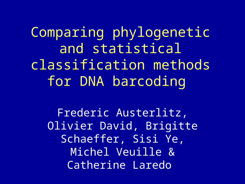
Testing the assignation methods

• Individual to be tested:– X1 : ATATGTACCTAGTA

– X2 : TTATCTACCTAGAA

• Reference sample :– 1_1: ATATGTACGTAGTA

– 1_2: ATATCTACGAAGTA

– 1_3: ATATCTACTAAGTA

– 2_1: ATATGTACGTAGTT

– 2_2: ATATGTACGAAGTT

– 2_3: ATTTCTACTAAGTT

Species 1

Species 2

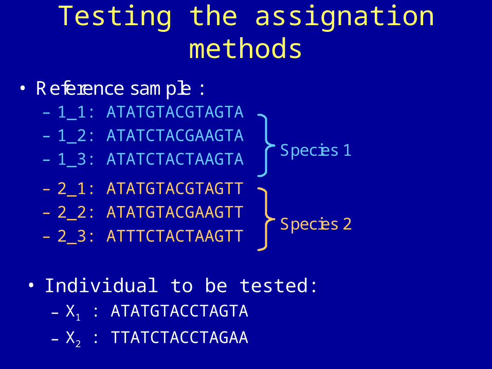
Phylogenetic methods

1_1 1_3 2_1 1_2 2_2 2_3X1

• Unanimity rule: X1 classified as ambiguous, X2 classified as species 1

• Majority rule: X1 and X2 classified as belonging to species 1

• Two methods tested: neighbor joining and maximum likelihood (PhyML, Guindon and Gascuel 2003)

X2

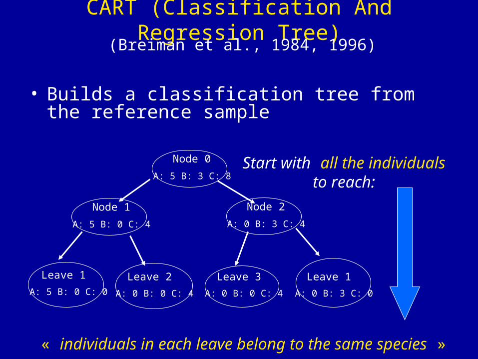
Node 0 Start with all the individualsto reach:

« individuals in each leave belong to the same species »

A: 5 B: 3 C: 8

CART (Classification And Regression Tree)

• Builds a classification tree from the reference sample

(Breiman et al., 1984, 1996)

Node 1

A: 5 B: 0 C: 4

Node 2

A: 0 B: 3 C: 4

Leave 1

A: 5 B: 0 C: 0

Leave 2

A: 0 B: 0 C: 4

Leave 3

A: 0 B: 0 C: 4

Leave 1

A: 0 B: 3 C: 0

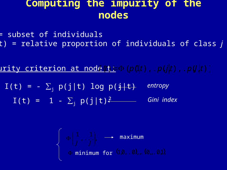
node t = subset of individualsp (j | t) = relative proportion of individuals of class j in node t

JJ

1,...,

1 maximum

1,0,...,0,...,0,...,0,1 minimum for

Computing the impurity of the nodes

Impurity criterion at node t:

I(t) = - ∑j p(j|t) log p(j|t) entropy

I(t) = 1 - ∑j p(j|t)² Gini index

))(),...,(),...,1(()( tJptjptptI

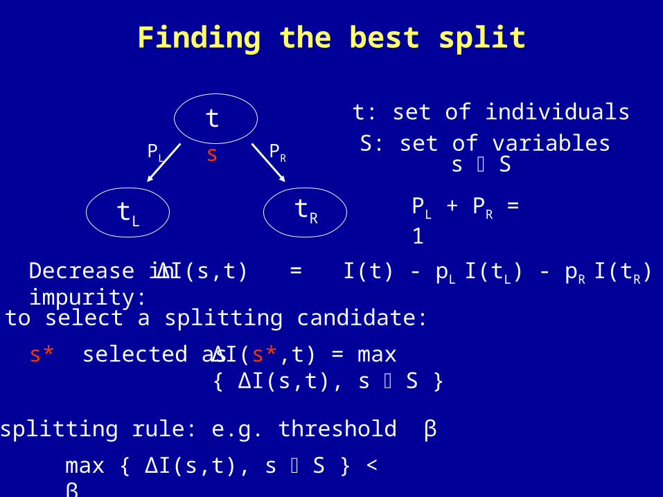
PL + PR = 1

t

tLtR

s PRPL s SS: set of variables

t: set of individuals

Finding the best split

ΔI(s*,t) = max { ΔI(s,t), s S }

ΔI(s,t) = I(t) - pL I(tL) - pR I(tR)

Rule to select a splitting candidate:

Decrease in impurity:

s* selected as

Stop splitting rule: e.g. threshold β

max { ΔI(s,t), s S } < β

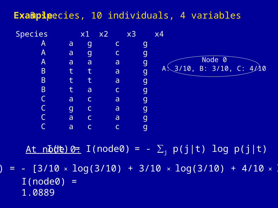
Example:

I(t) = I(node0) = - ∑j p(j|t) log p(j|t)At node 0:

I(node0) = - [3/10 × log(3/10) + 3/10 × log(3/10) + 4/10 × log(4/10)]

3 species, 10 individuals, 4 variables

I(node0) = 1.0889

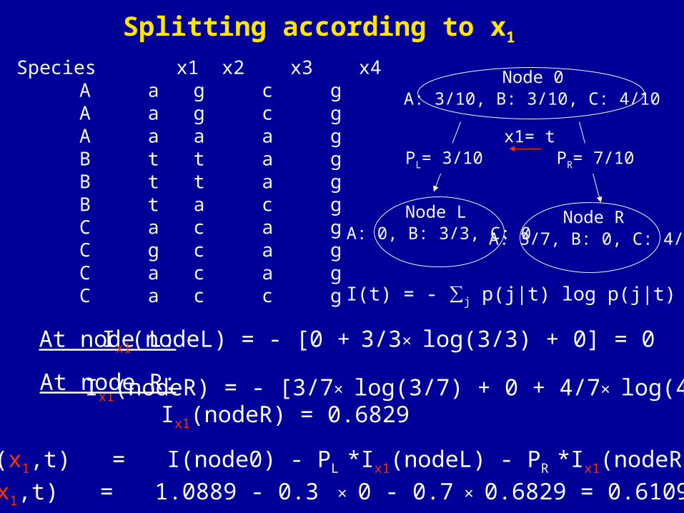
Species x1 x2 x3 x4 A a g c g A a g c g A a a a g B t t a g B t t a g B t a c g C a c a g C g c a g C a c a g C a c c g

Node 0A: 3/10, B: 3/10, C: 4/10

I(t) = - ∑j p(j|t) log p(j|t)

Splitting according to x1

Species x1 x2 x3 x4 A a g c g A a g c g A a a a g B t t a g B t t a g B t a c g C a c a g C g c a g C a c a g C a c c g

At node L: Ix1(nodeL) = - [0 + 3/3× log(3/3) + 0] = 0

Ix1(nodeR) = - [3/7× log(3/7) + 0 + 4/7× log(4/7)]At node R:

Ix1(nodeR) = 0.6829

A: 0, B: 3/3, C: 0 A: 3/7, B: 0, C: 4/7

Node 0A: 3/10, B: 3/10, C: 4/10

x1= t

Node L Node R

PR= 7/10PL= 3/10

ΔI(x1,t) = I(node0) - PL *Ix1(nodeL) - PR *Ix1(nodeR)

ΔI(x1,t) = 1.0889 - 0.3 × 0 - 0.7 × 0.6829 = 0.6109

I(t) = - ∑j p(j|t) log p(j|t)

At node L:

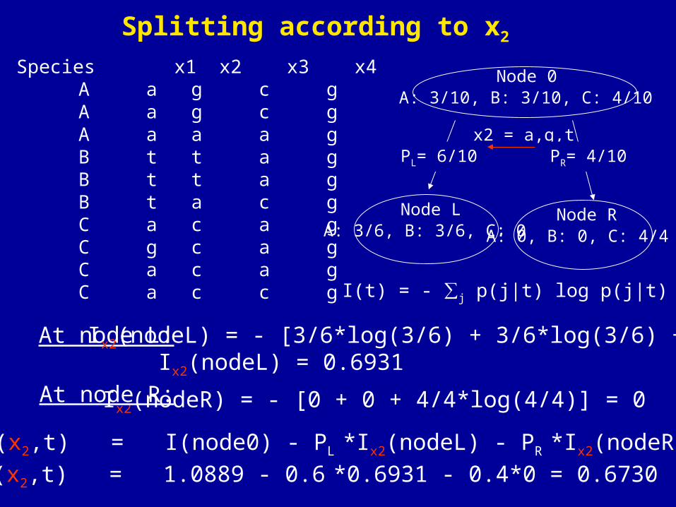
Ix2(nodeR) = - [0 + 0 + 4/4*log(4/4)] = 0

Species x1 x2 x3 x4 A a g c g A a g c g A a a a g B t t a g B t t a g B t a c g C a c a g C g c a g C a c a g C a c c g

Ix2(nodeL) = - [3/6*log(3/6) + 3/6*log(3/6) +0]

At node R:

Node 0A: 3/10, B: 3/10, C: 4/10

x2 = a,g,t

Node L Node RA: 3/6, B: 3/6, C: 0 A: 0, B: 0, C: 4/4

PR= 4/10PL= 6/10

ΔI(x2,t) = I(node0) - PL *Ix2(nodeL) - PR *Ix2(nodeR)

ΔI(x2,t) = 1.0889 - 0.6 *0.6931 - 0.4*0 = 0.6730

Ix2(nodeL) = 0.6931

Splitting according to x2

I(t) = - ∑j p(j|t) log p(j|t)

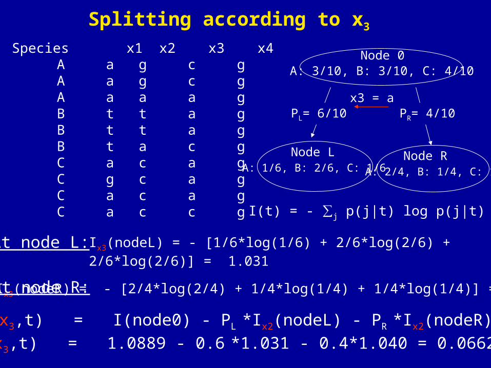
Ix3(nodeR) = - [2/4*log(2/4) + 1/4*log(1/4) + 1/4*log(1/4)] = 1.040

Species x1 x2 x3 x4 A a g c g A a g c g A a a a g B t t a g B t t a g B t a c g C a c a g C g c a g C a c a g C a c c g

At node L: Ix3(nodeL) = - [1/6*log(1/6) + 2/6*log(2/6) + 2/6*log(2/6)] = 1.031

At node R:

Node 0A: 3/10, B: 3/10, C: 4/10

x3 = a

Node L Node RA: 1/6, B: 2/6, C: 1/6 A: 2/4, B: 1/4, C: 1/4

PR= 4/10PL= 6/10

ΔI(x3,t) = I(node0) - PL *Ix2(nodeL) - PR *Ix2(nodeR)

ΔI(x3,t) = 1.0889 - 0.6 *1.031 - 0.4*1.040 = 0.0662

Splitting according to x3

Species x1 x2 x3 x4 A a g c g A a g c g A a a a g B t t a g B t t a g B t a c g C a c a g C g c a g C a c a g C a c c g

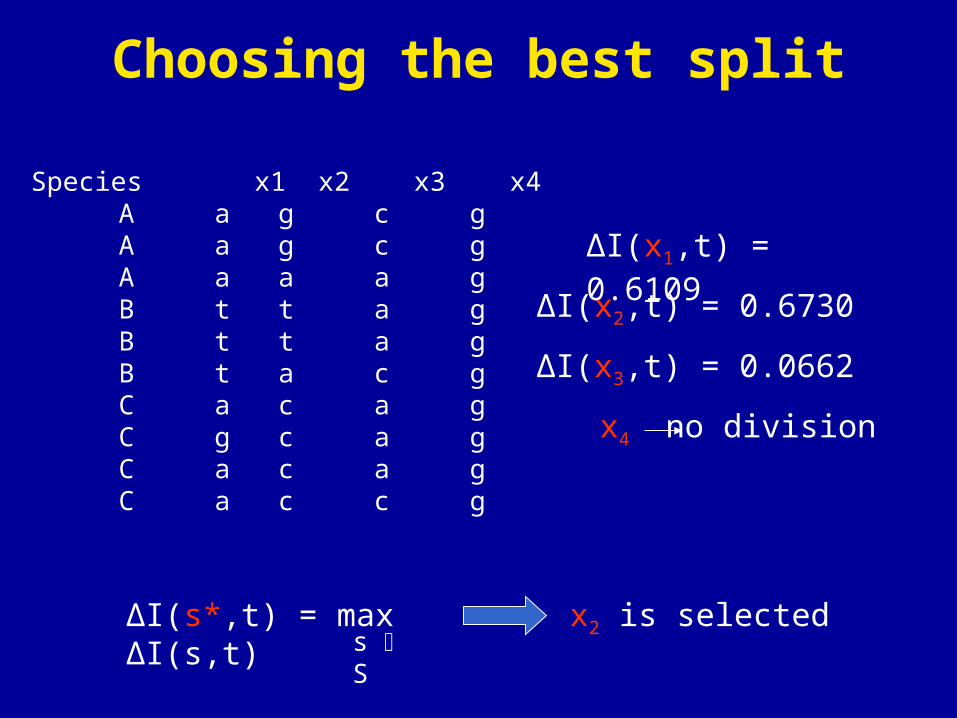
ΔI(x2,t) = 0.6730

ΔI(s*,t) = max ΔI(s,t)s S

ΔI(x1,t) = 0.6109

ΔI(x3,t) = 0.0662

x4 no division

x2 is selected

Choosing the best split

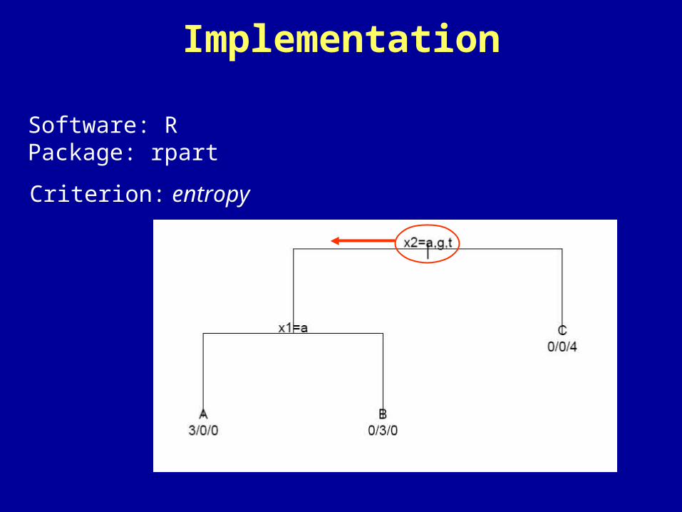
Criterion: entropy

Software: RPackage: rpart

Implementation

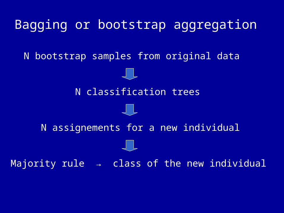
Bagging or bootstrap aggregation

N bootstrap samples from original data

N classification trees

N assignements for a new individual

Majority rule → class of the new individual

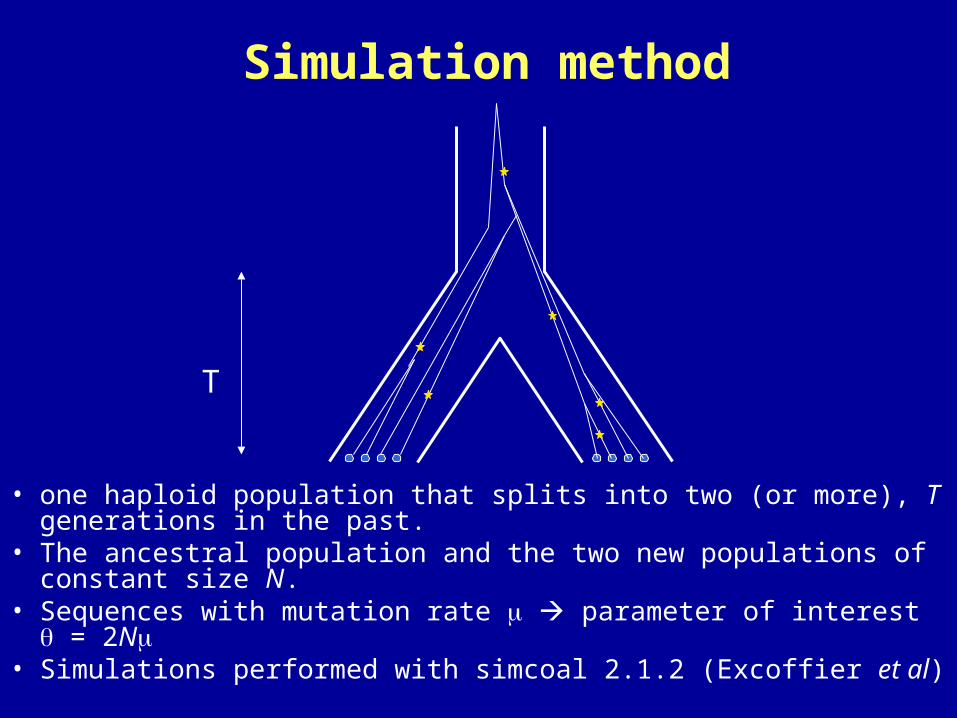
Simulation method

• one haploid population that splits into two (or more), T generations in the past.

• The ancestral population and the two new populations of constant size N.

• Sequences with mutation rate parameter of interest = 2N• Simulations performed with simcoal 2.1.2 (Excoffier et al)

T

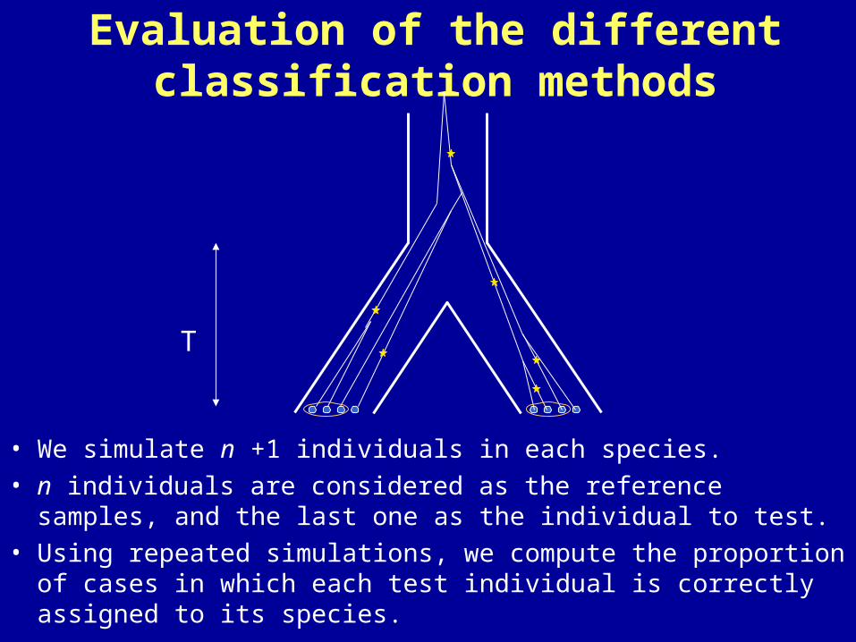
Evaluation of the different classification methods

• We simulate n +1 individuals in each species.

• n individuals are considered as the reference samples, and the last one as the individual to test.

• Using repeated simulations, we compute the proportion of cases in which each test individual is correctly assigned to its species.

T

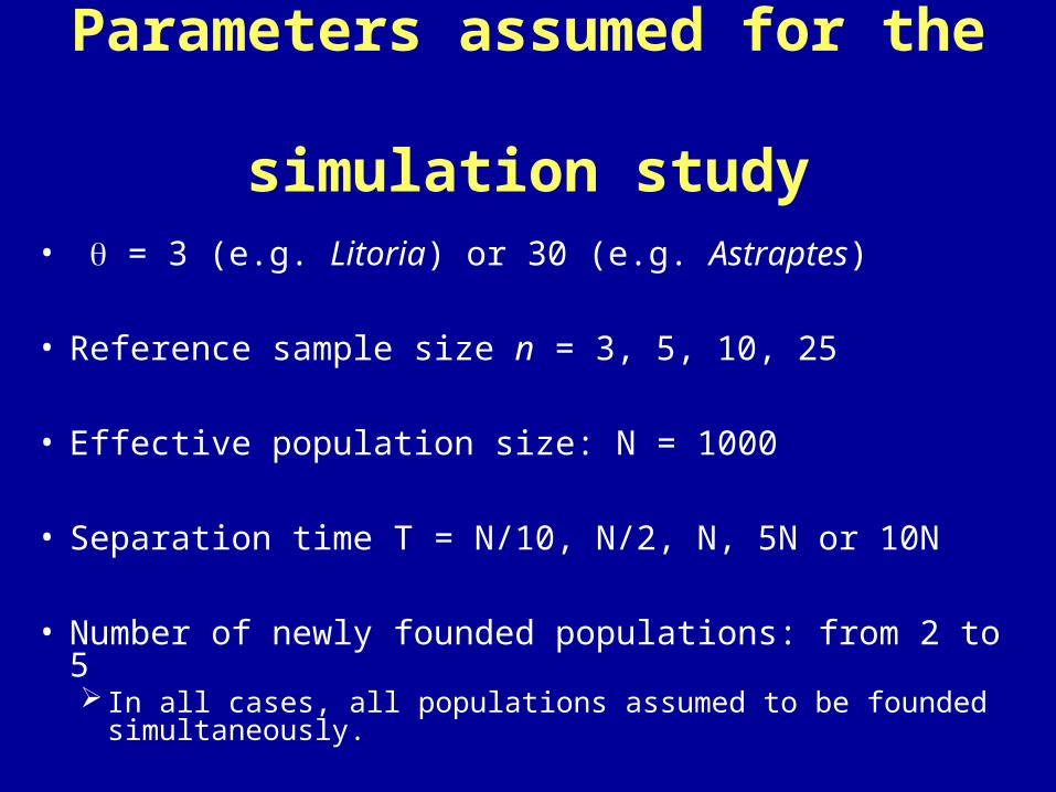
Parameters assumed for the simulation study

• = 3 (e.g. Litoria) or 30 (e.g. Astraptes)

• Reference sample size n = 3, 5, 10, 25

• Effective population size: N = 1000

• Separation time T = N/10, N/2, N, 5N or 10N

• Number of newly founded populations: from 2 to 5 In all cases, all populations assumed to be founded

simultaneously.

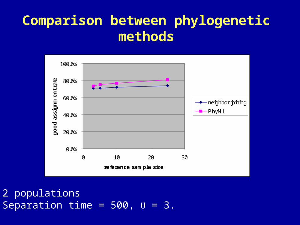
Comparison between phylogenetic methods

0.0%

20.0%

40.0%

60.0%

80.0%

100.0%

0 10 20 30

reference sample size

go

od

ass

ign

men

t ra

te

neighbor joining

PhyML

• 2 populations • Separation time = 500, = 3.

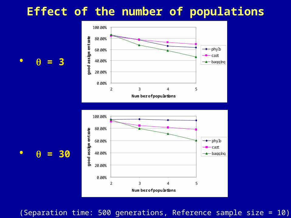
Effect of the number of populations

• = 3

0.00%

20.00%

40.00%

60.00%

80.00%

100.00%

2 3 4 5

Number of populations

go

od

ass

igm

ent

rate

phylo

cart

bagging

• = 30

0.00%

20.00%

40.00%

60.00%

80.00%

100.00%

2 3 4 5

Number of populations

go

od

ass

igm

ent

rate

phylo

cart

bagging

(Separation time: 500 generations, Reference sample size = 10)

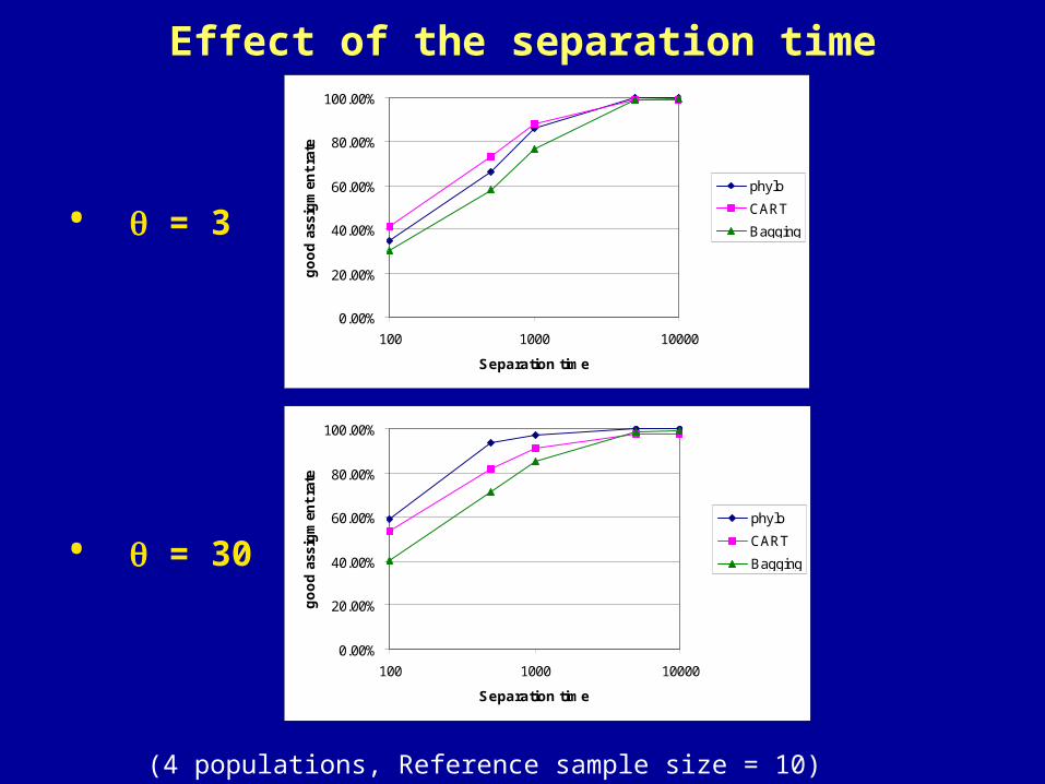
Effect of the separation time

• = 3

• = 30

(4 populations, Reference sample size = 10)

0.00%

20.00%

40.00%

60.00%

80.00%

100.00%

100 1000 10000

Separation time

go

od

ass

igm

ent

rate

phylo

CART

Bagging

0.00%

20.00%

40.00%

60.00%

80.00%

100.00%

100 1000 10000

Separation time

go

od

ass

igm

ent

rate

phylo

CART

Bagging

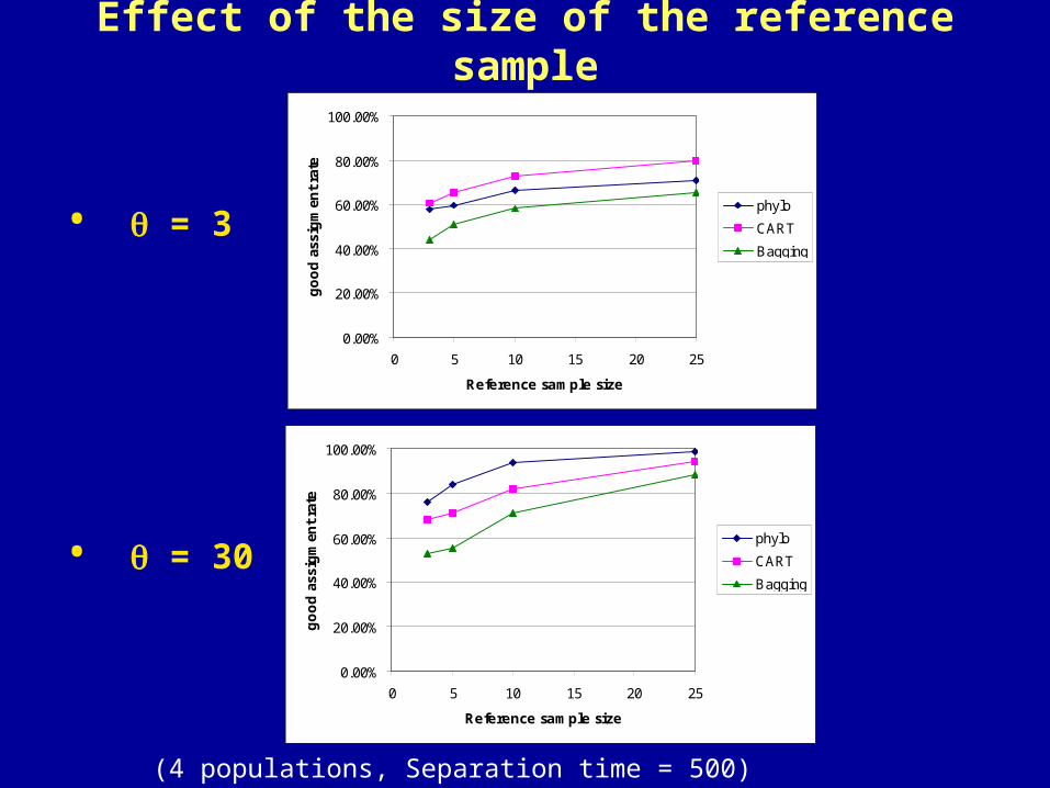
Effect of the size of the reference sample

• = 3

• = 30

(4 populations, Separation time = 500)

0.00%

20.00%

40.00%

60.00%

80.00%

100.00%

0 5 10 15 20 25

Reference sample size

go

od

ass

igm

ent

rate

phylo

CART

Bagging

0.00%

20.00%

40.00%

60.00%

80.00%

100.00%

0 5 10 15 20 25

Reference sample size

go

od

ass

igm

ent

rate

phylo

CART

Bagging

Adding nuclear genes

• We considered the case where polymorphism of nuclear genes are also available.

• We assumed that– these genes were independent.– they all have the same (= 4N) value, equal

to the value for the cytoplasmic genes.– They do not show intragenic recombination or

they show it at a rate equal to the mutation rate (c = , i.e. 4Nc = ).

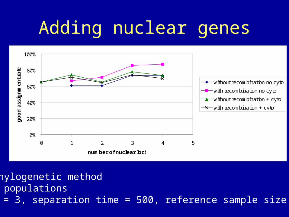
Adding nuclear genes

• Phylogenetic method• 2 populations• = 3, separation time = 500, reference sample size = 10

0%

20%

40%

60%

80%

100%

0 1 2 3 4 5

number of nuclear loci

go

od

ass

ign

men

t ra

te

without recombination no cyto

with recombination no cyto

without recombination + cyto

with recombination + cyto

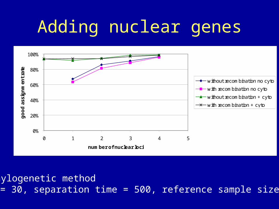
Adding nuclear genes

• Phylogenetic method• = 30, separation time = 500, reference sample size = 10

0%

20%

40%

60%

80%

100%

0 1 2 3 4 5

number of nuclear loci

go

od

ass

ign

men

t ra

te

without recombination no cyto

with recombination no cyto

without recombination + cyto

with recombination + cyto

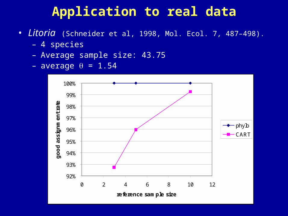
Application to real data

• Litoria (Schneider et al, 1998, Mol. Ecol. 7, 487–498).

– 4 species– Average sample size: 43.75– average = 1.54

92%

93%

94%

95%

96%

97%

98%

99%

100%

0 2 4 6 8 10 12

reference sample size

go

od

ass

ign

men

t ra

te

phylo

CART

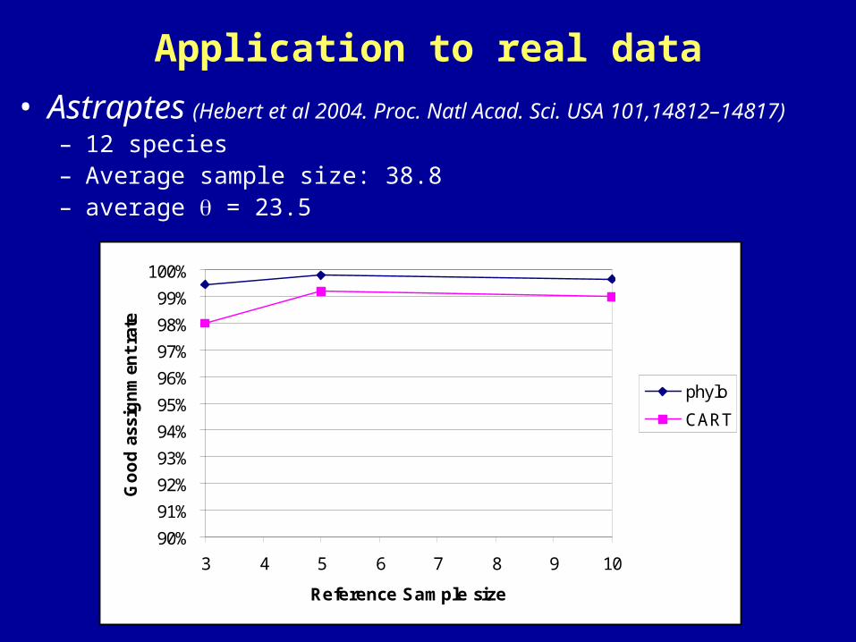
Application to real data

• Astraptes (Hebert et al 2004. Proc. Natl Acad. Sci. USA 101,14812–14817)

– 12 species– Average sample size: 38.8– average = 23.5

90%

91%

92%

93%

94%

95%

96%

97%

98%

99%

100%

3 4 5 6 7 8 9 10

Reference Sample size

Go

od

ass

ign

men

t ra

te

phylo

CART

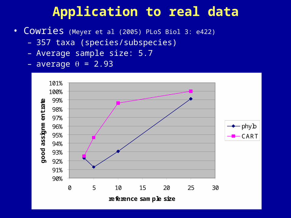
Application to real data• Cowries (Meyer et al (2005) PLoS Biol 3: e422)

– 357 taxa (species/subspecies)– Average sample size: 5.7– average = 2.93

90%91%92%

93%94%95%96%97%98%

99%100%101%

0 5 10 15 20 25 30

reference sample size

go

od

ass

ign

men

t ra

te

phylo

CART

Conclusions• Regarding phylogenetic methods, the maximum

likelihood method performs better than the neighbor joining.

• CART performs better than phylogenetic methods for poorly informative data (low value)

• but not for more polymorphic data (high value)

• Adding nuclear loci can help, but at a quite high cost.

• Recombination improves the phylogenetic method for low values (Ongoing work for CART).

Perspectives

• Developing a statistical method to put a confidence level on a given assignation.

• Evaluating other classification methods (learning methods)