Embed Size (px)
Citation preview

COMPARING MEASURED AND SIMULATED
BUILDING ENERGY PERFORMANCE DATA
A DISSERTATION
SUBMITTED TO THE DEPARTMENT OF
CIVIL AND ENVIRONMENTAL ENGINEERING
AND THE COMMITTEE ON GRADUATE STUDIES
OF STANFORD UNIVERSITY
IN PARTIAL FULFILLMENT OF THE REQUIREMENTS
FOR THE DEGREE OF
DOCTOR OF PHILOSOPHY
Tobias Maile
August 2010

This dissertation is online at: http://purl.stanford.edu/mk432mk7379
© 2010 by Tobias Maile. All Rights Reserved.
Re-distributed by Stanford University under license with the author.
ii

I certify that I have read this dissertation and that, in my opinion, it is fully adequatein scope and quality as a dissertation for the degree of Doctor of Philosophy.
Martin Fischer, Primary Adviser
I certify that I have read this dissertation and that, in my opinion, it is fully adequatein scope and quality as a dissertation for the degree of Doctor of Philosophy.
John Haymaker
I certify that I have read this dissertation and that, in my opinion, it is fully adequatein scope and quality as a dissertation for the degree of Doctor of Philosophy.
Vladimir Bazjanac
Approved for the Stanford University Committee on Graduate Studies.
Patricia J. Gumport, Vice Provost Graduate Education
This signature page was generated electronically upon submission of this dissertation in electronic format. An original signed hard copy of the signature page is on file inUniversity Archives.
iii
Tobias Maile
iv
Abstract
Finding building energy performance problems is a critical step in improving energy efficiency in
buildings and in reaching a building’s performance goals established during design. The prevalent
method of improving building energy performance is to look for relative improvements on the basis of
measured performance data, sometimes with a “calibrated” energy simulation model that is made to
mimic the actual consumption as closely as possible. This approach is problematic because
compensation errors often mask the performance problems one wants to find, a true baseline model is
not established, and there is little certainty that the identified improvements capture all major
performance problems. Typically, these assessment methods focus on either the building/system level
or the component level, but do not consider all levels of detail. Furthermore, existing methods do not
combine spatial and thermal perspectives and do not consider the relationships between components of
a building’s energy system, the HVAC (heating, ventilation, and air conditioning) systems, HVAC
components, zones, spaces, and the building. However, improving this interaction, i.e., using the energy
system for maximum effect in a building’s spaces, is precisely what building operators and users are
after. The effect of these shortcomings is that identification of energy performance problems tends to be
haphazard and requires great effort.
To address these gaps in knowledge and corresponding shortcomings, I formalized the Energy
Performance Comparison Methodology (ECPM) to identify performance problems from a comparison
of measured and simulated energy performance data. It extends prior hierarchies to describe a building
and its energy system more fully so that the comparison and analysis includes the spatial and thermal
perspectives and all levels of detail in a building, including the relevant relationships. It formalizes
measurement assumptions and simulations assumptions, approximations, and simplifications (AAS) so
that measured and simulated data can be assessed while considering all known limitations.
This thesis describes this EPCM and its related contributions to knowledge. It also shows that a
professional, called performance assessor, can identify more problems with less effort per problem than
with existing methods. The assessor uses whole building energy performance simulation (BEPS) tools,
such as EnergyPlus, to generate simulated data sets for the EPCM. Measured data come from physical
measurements by sensors strategically placed in buildings and control data points such as set points. By
enabling a meaningful comparison of measured and simulated data, this thesis enables future research to
establish expert systems that can automatically detect performance problems and correct them, allow
the virtual testing of energy efficiency improvements and innovations, and provide feedback to building
designers and operators for ongoing improvement of the design and building operations methods.

Tobias Maile
v
Acknowledgments
Due to my interest in advancing technology, I was always striving for higher educational goals, leading
to my pursue of a Ph.D. To achieve the goal of earning a Ph.D. would not have been possible without
the guidance, support, and motivation of several people, to whom I want to express my gratitude.
First of all, I want to acknowledge my committee members. First is Martin Fischer, my Ph.D. advisor,
who was interested in my research from the first time I met him. I am grateful for his support to find
case studies and to establish connections with the industry, as well as his guidance throughout the Ph.D.
process, including all the difficult questions he asked and his invaluable feedback to my papers. I want
to especially thank Vladimir Bazjanac for his involvement and guidance throughout my dissertation
research as well as for his encouragement to start one in the first place. I also want to thank John
Haymaker for his insights and comments to my papers and for his guidance and discussions early on
during my research. Last but not least on my committee, I want to thank Michal Lepech for his great
comments at my defense and discussion about the difference between dissertational contributions and
engineering work.
I want to thank Phillip Haves for his guidance and insights while working on the San Francisco Federal
Office building project and other projects through my involvement at EETD. Insights from Fred Buhl
about EnergyPlus concepts “under the hood” were helpful for my work, as well as various discussions
with Michael Wetter about current problems and possible future developments in building simulation. I
also enjoyed assisting Allan Daly in teaching fundamentals about HVAC systems and simulation
through sharing my knowledge with students, which triggered my interest in teaching. In addition, I
want to thank Tammy Goodall and Teddie Guenzer for their administrative support over the years as
well as everybody involved in providing access to facilities, documentation and of course measured
data of buildings. I would have not been able to accomplish this work without the daily support of my
colleagues at CIFE and EETD. In particular, I want to express my gratitude to James O’Donnell, who
has not only provided uncounted advice and support throughout the Ph.D. process, but also has become
a good friend. In addition, I want to thank the following people at CIFE: Caroline Clevenger, Timo
Hartmann, Mauricio Toledo, Claudio Mourgues, Peggy Ho, Benjamin Welle, Victor Gane, Reid
Senescu, Matt Garr, Christina Liebner, Tyler Haak, and Kathryn Megna. The following people from
EETD supported my work and thinking: Davide Dell Oro, Andrea Costa, Giorgio Pansa, Paul Raftery,
and Cody Rose.
Finally, I want to thank my family and friends for their support. It was always great to come back home
and take some time away from the academic work. My parents’ support and openness to let me explore
my opportunities and pursue an academic career at the “other end” of the world have been a
fundamental basis for my Ph.D. journey. I also want to express my gratitude to my siblings for their
understanding and willingness to keep up with new challenges arising from my doctoral studies. In

Tobias Maile
vi
particular, the unconditional love of my “little” brother Jonathan kept me going when times were
difficult. Last and certainly not least, I want to express my deepest gratitude to my wife Silke, who
always stood by me during this incredible journey. Her patience throughout the process has been
extraordinary, despite the countless extensions of my stay in the United States. Her understanding of my
pursuit of a Ph.D., her commitment to our relationship, and her love were fundamental during hard but
also good times. I dedicate my dissertation to her and our unborn child.
Tobias Maile
vii
Table of Contents
Abstract ........................................................................................................................ iv
Acknowledgments......................................................................................................... v
Table of Contents........................................................................................................vii
List of Tables..............................................................................................................xiii
List of Illustrations ....................................................................................................xiv
Chapter 1: Introduction............................................................................................... 1
1 Introduction ......................................................................................................................1
2 Comparison methods in other industries .......................................................................4
3 Research questions and theoretical points of departure...............................................5
3.1 How can a comparison of measured and simulated energy performance data identify
performance problems? ...............................................................................................6
3.2 How must spatial and HVAC building objects be represented to enable this
comparison? ................................................................................................................7
3.3 What measurement assumptions help to explain differences between measured and
simulated data? ............................................................................................................8
3.4 What simulation approximations, assumptions, and simplifications help to explain
differences between measured and simulated data?....................................................8
4 Research method...............................................................................................................8
5 Contributions ..................................................................................................................11
5.1 Energy Performance Comparison Methodology.......................................................11
5.1.1 Link to design BEPS models ...........................................................................................12
5.1.2 Increased level of detail...................................................................................................12
5.1.3 Bottom-up comparison ....................................................................................................12 5.1.4 Structured and iterative process.......................................................................................12
5.2 Building object hierarchy ..........................................................................................13
5.3 List of measurement assumptions and simulation AAS............................................14
6 Format of the Dissertation .............................................................................................14
7 References........................................................................................................................15
Tobias Maile
viii
Chapter 2: A method to compare measured and simulated data to assess building
energy performance.................................................................................................... 18
1 Abstract ...........................................................................................................................18
2 Introduction ....................................................................................................................18
3 Development of the EPCM ............................................................................................20
3.1 Research method: case studies ..................................................................................20
3.2 Selection of case studies............................................................................................21
3.3 Early comparisons .....................................................................................................22
3.4 Existing methods to detect performance problems ...................................................22
4 Energy Performance Comparison Methodology (EPCM)..........................................24
4.1 Updating simulation input .........................................................................................26
4.2 Building object hierarchy ..........................................................................................28
4.3 Process of identifying performance problems with the knowledge of measurement
assumptions and simulation AAS .............................................................................31
4.4 Iterative adjustment of the BEPS model ...................................................................32
5 Results of applying the EPCM ......................................................................................35
6 Validation ........................................................................................................................39
6.1 Validation of the building object hierarchy...............................................................40
6.2 Validation of the EPCM............................................................................................40
7 Limitations and future research....................................................................................42
7.1 Estimating impact on thermal comfort and energy consumption .............................42
7.2 Feedback based on identified performance problems ...............................................43
7.3 Better integration with controls.................................................................................43
7.4 Automation of EPCM................................................................................................43
7.5 Real-time energy performance assessment ...............................................................44
8 Conclusion .......................................................................................................................44
9 Bibliography....................................................................................................................45
Chapter 3: Formalizing assumptions to document limitations of building
performance measurement systems.......................................................................... 49
1 Abstract ...........................................................................................................................49
2 Introduction ....................................................................................................................49
3 Measurement systems and their limitations.................................................................52
3.1 Existing measurement data sets.................................................................................52
Tobias Maile
ix
3.1.1 Utility data set..................................................................................................................56
3.1.2 HVAC control data set ....................................................................................................56
3.1.3 Guidelines for the Evaluation of Building Performance .................................................56
3.1.4 Procedure for Measuring and Reporting Commercial Building Energy Performance....57 3.1.5 Guide for Specifying Performance Monitoring Systems in Commercial and Institutional
Buildings.........................................................................................................................57
3.1.6 Ideal data set and actor view ...........................................................................................57
3.1.7 Summary of measurement data sets ................................................................................59
3.2 Selecting data points for performance evaluation .....................................................59
3.3 Sensor accuracy.........................................................................................................60
3.4 Data transmission ......................................................................................................62
3.5 Data archiving ...........................................................................................................63
3.6 Process of identifying performance problems with the knowledge of measurement
assumptions ...............................................................................................................63
3.7 Measurement assumptions ........................................................................................64
3.8 Verification of the functionality of a measurement system ......................................67
3.9 Reliability of a measurement system ........................................................................69
4 Case studies .....................................................................................................................69
4.1 Case study 1: San Francisco Federal Building (SFFB).............................................70
4.1.1 Building description ........................................................................................................70 4.1.2 Measurement data set ......................................................................................................71
4.1.3 Data acquisition system...................................................................................................72
4.2 Case study 2: Global Ecology Building (GEB) ........................................................73
4.2.1 Building description ........................................................................................................73
4.2.2 Measurement data set ......................................................................................................74
4.2.3 Data acquisition system...................................................................................................74
4.3 Case study 3: Yang and Yamazaki Environment and Energy Building (Y2E2) ......75
4.3.1 Building description ........................................................................................................75
4.3.2 Measurement data set ......................................................................................................76
4.3.3 Data acquisition system...................................................................................................77
4.4 Case study 4: Santa Clara County Building (SCC)...................................................79
4.4.1 Building description ........................................................................................................79 4.4.2 Measurement data set ......................................................................................................80
4.4.3 Data acquisition system...................................................................................................81
4.5 Summary of measurement data sets ..........................................................................82
Tobias Maile
x
4.6 Reliability measure of case studies ...........................................................................84
5 Validation ........................................................................................................................84
5.1 Validation of measurement data sets.........................................................................85
5.2 Validation of measurement assumptions...................................................................86
6 Recommendations...........................................................................................................87
6.1 Select appropriate sensors based on existing measurement guidelines.....................87
6.2 Use more thorough sensor calibration.......................................................................87
6.3 Design control systems that support continuous data archiving ...............................87
6.4 Use local solar data measurements............................................................................89
7 Limitations and future research....................................................................................89
7.1 Validation of measurement guidelines ......................................................................89
7.2 Identification of an expanded assumption list...........................................................90
7.3 Development of case studies with more measurements............................................90
7.4 Testing of manufacturer accuracy of sensors ............................................................90
8 Conclusion .......................................................................................................................91
9 Bibliography....................................................................................................................91
Chapter 4: Formalizing approximations, assumptions, and simplifications to
document limitations in building energy performance simulation........................ 96
1 Abstract ...........................................................................................................................96
2 Introduction ....................................................................................................................96
3 BEPS and its AAS...........................................................................................................98
3.1 Semi-automated creation of simulation input data....................................................99
3.2 Accuracy of simulation results ................................................................................102
3.3 Identification of simulation assumptions, approximations, and simplifications .....103
3.4 Process to identify performance problems from differences ..................................106
4 Selection of EnergyPlus as appropriate BEPS tool ...................................................107
4.1 Requirements for BEPS tools for use during building operation............................107
4.2 Existing whole building energy performance simulation tools...............................110
4.3 Selection of EnergyPlus ..........................................................................................111
5 EnergyPlus and its AAS in case studies......................................................................112
5.1 Case study 1: San Francisco Federal Building (SFFB)...........................................112
5.1.1 HVAC system................................................................................................................112
5.1.2 Design BEPS model ......................................................................................................113
Tobias Maile
xi
5.1.3 Usage approximations, assumptions, and simplifications.............................................113
5.2 Case study 2: Global Ecology Building (GEB) ......................................................113
5.2.1 HVAC system................................................................................................................113
5.2.2 Design BEPS model ......................................................................................................114
5.2.3 Usage approximations, assumptions, and simplifications .............................................114
5.3 Case study 3: Yang and Yamazaki Environment and Energy Building (Y2E2) ....115
5.3.1 HVAC system................................................................................................................115 5.3.2 Design BEPS model ......................................................................................................116
5.3.3 Usage approximations, assumptions, and simplifications.............................................116
5.4 Case study 4: Santa Clara County Building (SCC).................................................119
5.4.1 HVAC system................................................................................................................119
5.4.2 Design BEPS model ......................................................................................................120
5.4.3 Usage approximations, assumptions, and simplifications.............................................120
6 Limitations of and recommendations for BEPS tools ...............................................121
6.1 Inadequate geometric representation.......................................................................122
6.2 Inability to model innovative, unique, and unorthodox objects, systems and
configurations..........................................................................................................123
6.2.1 Limited HVAC topology...............................................................................................123
6.2.1.1 Limited air loop supply branch configurations......................................................124
6.2.1.2 Limitations with zone equipment components.....................................................124
6.2.1.3 Limitation of water loop configuration .................................................................124
6.2.2 Representation of controls in EnergyPlus .....................................................................124
6.2.3 Missing HVAC components..........................................................................................125
6.3 Limitations for a comparison with measured data ..................................................126
6.3.1 Limited import of measured data ..................................................................................127 6.3.2 Model warm-up .............................................................................................................127
6.3.3 Report limitations ..........................................................................................................127
6.4 Limitations of internal data models for interoperability .........................................128
6.5 Graphical user interfaces .........................................................................................128
6.6 Increased level of detail...........................................................................................129
7 Validation of simulation AAS......................................................................................129
8 Limitations and future research..................................................................................131
8.1 Emerging technologies in simulation tools .............................................................131
8.2 Integration of error calculations into whole building simulation tools ...................131
8.3 An expert system based on approximations, assumptions, and simplifications......132

Tobias Maile
xii
8.4 Identifying new approximations, assumptions, and simplifications .......................132
8.5 Detailed analysis of accuracy of simulation results ................................................132
9 Conclusion .....................................................................................................................133
10 Bibliography..................................................................................................................133
Appendix A: Details about the analysis of measurement data sets...................... 139
Appendix B: List of measurement assumptions including anticipated effects ... 141
Appendix C: List of simulation AAS including anticipated effects ..................... 143
Tobias Maile
xiii
List of Tables
Table 2-1: Description of the three case studies.......................................................................................21 Table 2-2: Examples of events at Y2E2...................................................................................................34
Table 2-3: Y2E2 summary table of comparison result of set points after iteration 1 ..............................37
Table 2-4: Identified performance problems and problem instances at Y2E2 with EPCM.....................39
Table 2-5: Summary of identified problem instances at Y2E2 ................................................................42
Table 3-1: Summary of topics covered by each guideline .......................................................................54
Table 3-2: Summary of existing measurement data sets ..........................................................................55
Table 3-3: Categorization based on O’Donnell’s actor view of measurement data sets..........................58
Table 3-4: Summary of measurement data sets of case studies and guidelines .......................................83 Table 4-1: Approximated time effort for BEPS model creation for each case study.............................101
Table 4-2: Summary of number of building objects per case study.......................................................101
Table 4-3: BEPS tool evaluation based on requirements for use during operation ...............................111
Table 4-4: Measured variables without direct counterparts in simulation .............................................128
Table A-1: Necessary sensors to detect known performance problems.................................................139
Table A-2: Availability of necessary sensors for each measurement data set guideline .......................140 Table A-3: Count of known performance problems per percentage range of available sensors............140
Table B-1: Anticipated effects of measurement assumptions ................................................................141
Table C-1: Anticipated effects of simulation AAS ................................................................................143
Tobias Maile
xiv
List of Illustrations
Figure 1-1: Level of detail of a building ....................................................................................................1 Figure 1-2: Big picture of limitations in relation to comparisons of measured and simulated data ..........2
Figure 1-3: Overview of concepts ..............................................................................................................3
Figure 1-4: O’Donnell’s hierarchy in pyramid representation ...................................................................7
Figure 1-5: CIFE “horseshoe” research method.........................................................................................9
Figure 1-6: Overview of research methods and tasks ..............................................................................10
Figure 1-7: Overview of EPCM ...............................................................................................................13
Figure 1-8: Pyramid representation of building object hierarchy ............................................................14
Figure 2-1: Example comparison graphs from SFFB ..............................................................................22 Figure 2-2: Overview of existing performance comparison methods ......................................................23
Figure 2-3: Overview of Energy Performance Comparison Methodology..............................................25
Figure 2-4: Weather converter data flow .................................................................................................27
Figure 2-5: Pyramid view of building object hierarchy ...........................................................................29
Figure 2-6: Graphical EXPRESS representation of building object hierarchy ........................................30
Figure 2-7: Example of a partial building object hierarchy of Y2E2.......................................................30
Figure 2-8: Example comparison of airflow on the system and component level ...................................31
Figure 2-9: Process for using measurement assumptions and simulation AAS to detect performance
problems from differences between pairs of measured and simulated data ...................................32
Figure 2-10: BEPS model adjustment process .........................................................................................33
Figure 2-11: BEPS model adjustments and change events ......................................................................35
Figure 2-12: Iterations for the Y2E2 case study.......................................................................................36
Figure 3-1: Overview of different measurement data sets .......................................................................59
Figure 3-2: Process of selecting data points for performance evaluation ................................................60
Figure 3-3: Example comparison graph to illustrate error margins of measurements .............................61 Figure 3-4: Process for using measurement assumptions to detect performance problems from
differences between pairs of measured and simulated data ............................................................64
Figure 3-5: Comparison data pair graph: Window status atrium A&B 2nd floor .....................................66
Figure 3-6: Comparison data pair graph: Temperature heating set point for space 143 ..........................67
Figure 3-7: Process of setting up and verifying a data acquisition system ..............................................68
Figure 3-8: East view of the SFFB...........................................................................................................70
Figure 3-9: Plan and section view of the SFFB........................................................................................70
Figure 3-10: Plan view of sensor layout in the SFFB ..............................................................................71 Figure 3-11: Data acquisition system at the SFFB...................................................................................72
Figure 3-12: Southeast view of the GEB and plan view of the first floor of the GEB ............................73
Figure 3-13: Example schematic for hot water loop data points in the GEB...........................................74
Tobias Maile
xv
Figure 3-14: Data acquisition system at the GEB ....................................................................................75
Figure 3-15: Illustration and floor plan of second floor of the Y2E2 building ........................................76
Figure 3-16: Example schematic for hot water loop data points in the Y2E2 .........................................77
Figure 3-17: Data acquisition system of the Y2E2 ..................................................................................78 Figure 3-18: Northeast view of the SCC ..................................................................................................80
Figure 3-19: Example schematic for hot water loop data points in the SCC ...........................................81
Figure 3-20: Data acquisition system of the SCC ....................................................................................82
Figure 3-21: Monthly reliability measures of two case studies over time ...............................................84
Figure 3-22: Results from validation of existing measurement data sets with the Y2E2 ........................85
Figure 3-23: Occurrences of measurement assumptions in case studies and literature ...........................86
Figure 4-1: Creation of an EnergyPlus model........................................................................................100
Figure 4-2: Macro process for generating a complete EnergyPlus model file .......................................101 Figure 4-3: The process of using DOE-2 translator to generate an EnergyPlus input file.....................102
Figure 4-4: Process for using simulation AAS to detect performance problems from differences between
pairs of measured and simulated data ...........................................................................................106
Figure 4-5: Comparison example showing supply air temperature of an air-handling unit measured and
simulated .......................................................................................................................................107
Figure 4-6: SFFB HVAC schematic ......................................................................................................112
Figure 4-7: GEB HVAC schematic........................................................................................................114
Figure 4-8: GEB roof spray simplification (on chilled water supply side) ............................................115 Figure 4-9: Y2E2 HVAC schematic ......................................................................................................116
Figure 4-10: Y2E2 hot steam simplification ..........................................................................................117
Figure 4-11: Y2E2 loop connection simplification ................................................................................117
Figure 4-12: Y2E2 air loop topology simplification ..............................................................................118
Figure 4-13: Y2E2 air loop branching simplification ............................................................................118
Figure 4-14: Y2E2 simplification of zone equipment component configuration ..................................119
Figure 4-15: SCC HVAC schematic ......................................................................................................120 Figure 4-16: SCC HVAC air loop branch simplification.......................................................................121
Figure 4-17: SCC chilled water loop pump configuration .....................................................................121
Figure 4-18: Examples of complex geometrical configurations ............................................................122
Figure 4-19: Occurrences of simulation AAS in case studies and literature..........................................130
Chapter 1: Introduction Tobias Maile
1
Chapter 1: Introduction
1 Introduction Current U.S. federal legislation requires significant reduction of energy consumption in buildings. For
example, the Energy Independence and Security Act of 2007 requires that all new commercial buildings
have a zero-net-energy balance by 2025 and that all buildings do so by 2050 (Sissine 2007). In
designing buildings that comply with these requirements, building energy performance simulation
(BEPS) will provide the guidance to virtually test different design strategies. While designing buildings
that achieve these goals can be difficult, building and operating them so they actually perform to these
requirements is the real challenge. Several studies show that buildings do not perform as they were
simulated to do so during design (Scofield 2002; Piette et al. 2001; Persson 2005; Kunz et al. 2009). To
understand the reasons for these discrepancies between measured and simulated data, a method is
needed that highlights these discrepancies and helps to improve design BEPS models. The current
practice of assessing building performance is ad hoc and mostly based on available measured data, and
the comparison with design goals is often neglected. In addition, building designs are adopted without
ever considering the actual performance of the buildings. Thus, the feedback loop between design,
including the goals, decision, and assumptions made, and operation is rarely closed, prolonging
inefficient practices and slowing the pace of performance improvement and adoption of appropriate
innovations. Today’s assessment methods miss many performance problems due to the high effort to
detect problems. To compare different approaches to assessing building performance I use the number
of performance problems as well as the time effort involved in detecting each problem as metrics.
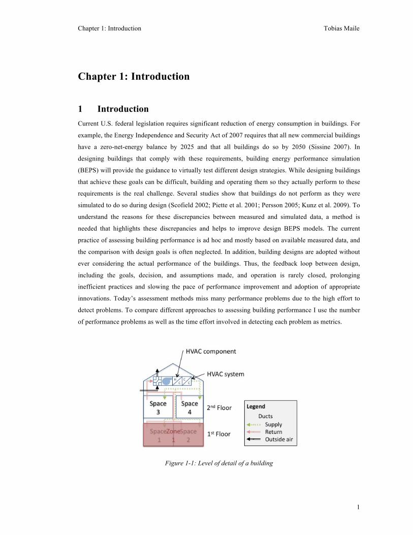
Figure 1-1: Level of detail of a building
Chapter 1: Introduction Tobias Maile
2
As illustrated in Figure 1-1, each building consists of a number of floors, which contain a number of
spaces. From a thermal perspective spaces are combined into so-called thermal zones. HVAC (heating,
ventilation and air conditioning) systems serve these thermal zones and consist of HVAC components.
Different assessment methods focus on different combinations of building objects. Calibration of BEPS
models is typically based on BEPS models created during design on building and system levels.
Calibrating a simulation model to achieve a predefined statistical characteristic (e.g., 5% error margin)
includes a fundamental shortcoming of these methods: the resulting calibrated model may include
compensation errors at the building level (Clarke 2001). For example, an oversized pump may
compensate for the error caused by an undersized fan. Thus, significant differences between the BEPS
model and the measured data may be hidden at the building level and can only be found if more detail is
included at the component level. Sun and Reedy (2006) describe the basic issue with calibrated models
as a problem that is underdetermined, which means that there are more input variables than there are
measured data. With the availability of more affordable measured data, the number of missing data
points can be reduced.
Calibrated simulation is often based on a top-down approach, which has the compensation error issue.
Hyvarinen and Karki (1996) describe a bottom-up approach, but they recommend a top-down approach
because of the unavailability of data at the bottom level. Since that paper was published, performance
data at the bottom (HVAC component) level has become increasingly available, and the bottom-up
approach is now feasible. This leads to the need for more detail in simulation models so that simulated
and actual/observed performance can be compared with fewer and smaller compensation errors.
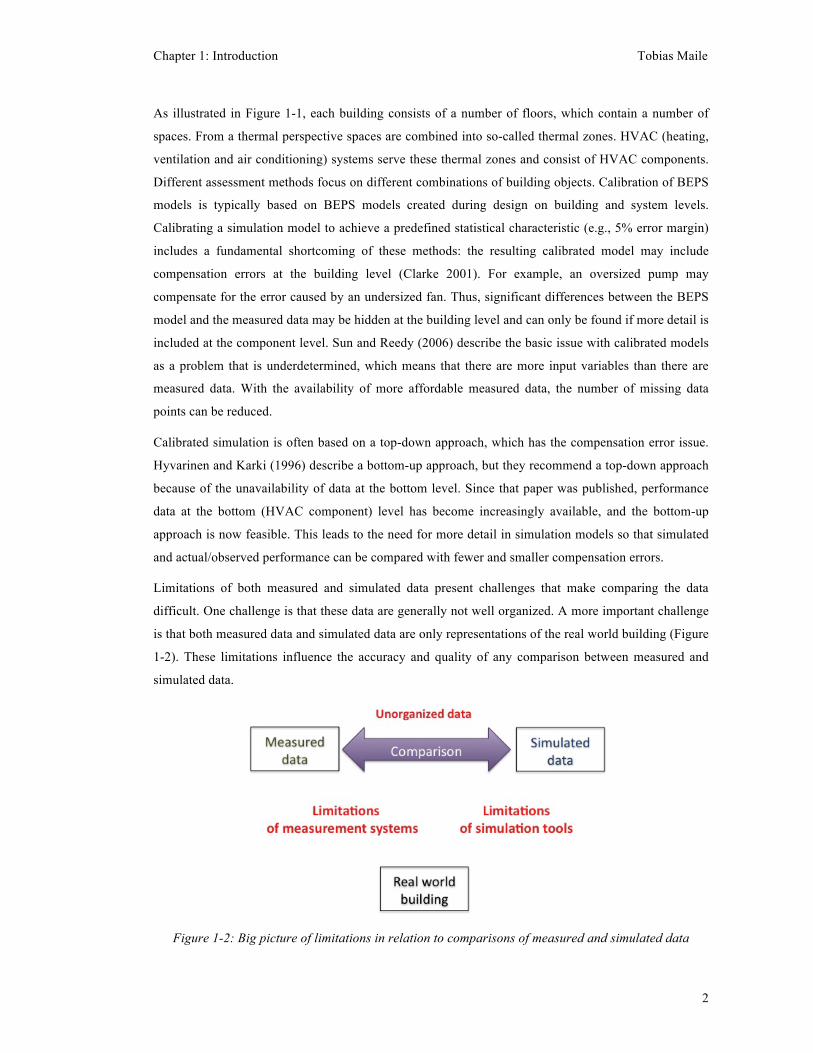
Limitations of both measured and simulated data present challenges that make comparing the data
difficult. One challenge is that these data are generally not well organized. A more important challenge
is that both measured data and simulated data are only representations of the real world building (Figure
1-2). These limitations influence the accuracy and quality of any comparison between measured and
simulated data.
Figure 1-2: Big picture of limitations in relation to comparisons of measured and simulated data
Chapter 1: Introduction Tobias Maile
3
A formal representation of building objects provides a structure to organize related measured and
simulated performance data in a meaningful way. Since measured performance data are linked to
HVAC systems and components but also to spatial objects, a representation that combines both
perspectives is necessary. O'Donnell (2009) developed such a representation that focuses on a thermal
perspective around the zone object. In this context a thermal zone is an agglomeration of building
spaces with similar thermal characteristics (e.g., lighting usage or occupancy). His representation does
not include space objects and follows a tree structure without relationships between different tree
branches (e.g., between water HVAC components and air HVAC components). These shortcomings of
his representation are due to his use of a zone-focused concept of assessing building performance.
Limitations of measurement systems are often loosely described using the error margins of sensors.
However, the measurement system consists not only of sensing components, but also of transmission
and archiving components. Limitations of all three functional aspects of measurement systems need to
be documented to better understand the representation of measured data.
Limitations of simulation tools influence the results and thus impact simulated performance data
significantly. These limitations are either embedded in the simulation tool or caused by the particular
use of a tool and included in input data. The documentation of these limitations is important for
understanding simulated performance data.
Figure 1-3: Overview of concepts
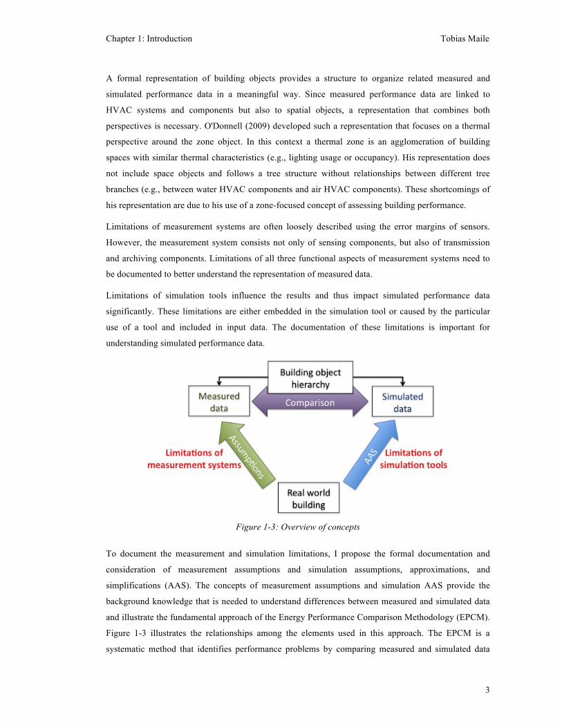
To document the measurement and simulation limitations, I propose the formal documentation and
consideration of measurement assumptions and simulation assumptions, approximations, and
simplifications (AAS). The concepts of measurement assumptions and simulation AAS provide the
background knowledge that is needed to understand differences between measured and simulated data
and illustrate the fundamental approach of the Energy Performance Comparison Methodology (EPCM).
Figure 1-3 illustrates the relationships among the elements used in this approach. The EPCM is a
systematic method that identifies performance problems by comparing measured and simulated data
Chapter 1: Introduction Tobias Maile
4
based on the developed building object hierarchy. A performance assessor, who is a HVAC engineer,
performs or supervises the tasks of the EPCM. This method specifically focuses on the performance
assessment of commercial buildings.
Previous research has introduced assumptions to explain differences between measured and simulated
data sporadically on a project-specific basis. An example of a measurement assumption is the use of
spot measurements that are representative of the actual quantity (Avery 2002). An example of
simulation AAS is the assumption that the air in zones is well-mixed (Gowri et al. 2009). With
knowledge of these measurement assumptions and simulation AAS, it is possible to assess differences
between measured and simulated data and explain whether a difference is plausible because of the
assumptions or whether it is a symptom of a performance problem.
The following subsections discuss the research questions I addressed in my Ph.D. studies and the
relevant theoretical points of departure. I provide details on the research method and the contributions
to knowledge and describe the format of this dissertation.
2 Comparison methods in other industries Other industries also use simulation to predict performance of products and compare simulation results
to measured data. The major differences between those products and buildings are highlighted by two
examples from the automotive and aerospace industries. For example, Nyberg (2002) describes a
model-based diagnostic method for evaluating an engine through extended prototype testing. The
prototype is equipped with 10 sensors to measure physical characteristics. During the prototype testing
only two external variables changed (engine speed and pressure); thus it is a controlled experiment and
thus not nearly as dynamic as building usage. In contrast to the building industry, the automotive
industry produces mass products and thus can spend significant effort in testing and prototyping of the
product. The small number of sensors indicates the small number of components that all operate within
one system. In contrast, in a building multiple systems, various components, spaces and occupants
interact resulting in a more complex system with many more sensors. The magnitude of the experiment
and the technical challenge allows a more detailed simulation that includes a small number of
assumptions of simulation models and measurements. These assumptions are published and their effect
discussed openly in the literature.
Schmid et al. (2007) investigated airflow characteristics of an open hatch of an airplane, which is a
rather atypical example for the aerospace industry. The CFD simulation results are compared with
measured data obtained during wind tunnel tests and during a test flight using 56 sensors. While this
airplane is also a unique product (designed to observe the stratospheric infrared spectrum), it has limited
external influences and user interaction and is tested before its intended use. The differences between
Chapter 1: Introduction Tobias Maile
5
measured and simulated performance data are mostly assigned to simulation assumptions and
simplifications.
Both studies focus on a specific aspect of a car or an airplane and do not consider the overall
performance of the complete product. Compared to the automotive and aerospace industries, the
building industry has some key differences that affect the use of comparisons between simulated and
measured data. Each building is a unique product because of its unique purpose and location that
consists of a complex system (needing hundreds or thousands of sensors) and has more external
influences (such as weather, occupancy, or changes to the building). Another important difference
between the building industry and the automotive and aerospace industries is that cars and airplanes
have significantly different functional requirements. For the security of the passengers, it is crucial that
airplanes do not fall out of the sky and cars do not leave the road and do not collide with obstacles.
Energy use in buildings, on the contrary, is seldom a safety issue, and failures of single HVAC
components or even of complete HVAC systems have less dramatic consequences. The smaller
significance of HVAC operation leads to less effort to ensure their proper operation. However, the
impact of buildings on green house gas emissions has been well document (Norman et al. 2006; Charles
2009; Walsh et al. 2009), heightening the urgency to understand building energy performance better
and improve it. Other industries that produce mass products create and thoroughly test prototypes
whereas the building industry cannot create prototypes since buildings are mostly unique products.
Thus, virtual prototyping is more important for buildings since it is not possible to build a physical
prototype for each building. Hence, these virtual prototypes need to become as good as possible to
enable a meaningful comparison with actual buildings.
3 Research questions and theoretical points of departure This dissertation answers the following four research questions:
1. How can a comparison of measured and simulated energy performance data identify
performance problems?
2. How must spatial and HVAC building objects be represented to enable this comparison?
3. What measurement assumptions help to explain differences between measured and simulated
data?
4. What simulation approximations, assumptions, and simplifications help to explain differences
between measured and simulated data?
The first question, which is also the main research question, addresses the methodology of how to
compare measured and simulated performance data to identify performance problems (chapter 2). This
question focuses on the comparison between results from BEPS models reflecting design and actual
measured data. The second question looks into how building objects must be represented to link
Chapter 1: Introduction Tobias Maile
6
measured and simulated data points and to reflect measurement assumptions and simulation AAS
accurately (chapter 2). The third and fourth research questions address the documentation of the
limitations of measurement systems (chapter 3) and simulation models with AAS (chapter 4). I discuss
each question and summarize points of departure for each research question in the following
subsections, and the answers to the four questions are the contributions of this dissertation research (see
section 5).
3.1 How can a comparison of measured and simulated energy performance
data identify performance problems? Several approaches exist in the broader area of comparing measured and simulated performance data.
Probably the most popular approach is the use of calibrated simulation models. Reddy (2006) provides
a literature review of existing calibration methods that aim to validate existing simulation models based
on measured data, obtained mainly on the building and system levels. While calibration methods
provide a link to design simulation models, they aim to achieve a match between measured and
simulated data within a predefined statistical criterion (e.g., 5% error margin). Design simulation
models are adjusted until the simulation results fall within this predefined range. This leads to the
possibility that there are multiple possible simulation models that all fall within the same error
tolerance. Thus, each of the simulation models itself is arbitrary and may or may not represent the
actual building. In particular, compensating errors on the building level may hide the fact that the
simulation model does not represent the actual performance but comes close, due to the existence of
performance problems that have offsetting effects (Clarke 2001). In addition, the measured performance
data may reflect significant performance problems in the building, and thus the simulation model would
be adjusted to match with these data, which masks the very performance problems building operators
and designers want to find. The resulting simulated data are not sufficiently independent from the
measured data, and thus they cannot be used as a reliable baseline.
Some calibration methods create simulation models based on existing design documentation instead of
using design simulation models. Salsbury and Diamond (2000) use this approach of basing the
simulation model on design documentation, but develop a simulation model specifically for a
comparison with measured data on the system level. Thus, Salsbury and Diamond describe the general
process of comparing measured and simulated data, but they do not provide a detailed and structured
methodology for doing so.
A fundamental issue with model calibration is that the problem is underdetermined (Sun and Reedy
2006), which means that there are more equations and thus unknown parameters than there are available
measured data. Various calibration methods aim to simplify the model calibration problem, but the
more promising approach is to include more detail to address this basic issue of the underdetermined
problem. Finally, most performance assessment methods (Austin 1997; Wang et al. 2005; Xu et al.

Chapter 1: Introduction Tobias Maile
7
2005; Seidl 2006) use a top-down approach to analyzing performance data. Because of the previously
mentioned compensation errors, problems may not be visible at the building or system level. Hyvarinen
and Karki (1996) mention the lack of availability of measured data at the bottom-up level (component
level) as a reason to use the top-down approach.
Assessment methods that are based on first principle methods (e.g., Augenbroe and Park 2005) do not
provide the beneficial link to design BEPS models. While such first principle methods may determine
areas of insufficient performance, they provide limited details about the specifics of a performance
problem. Furthermore, first principle models are limited in representing complex controls and the
interplay of multiple HVAC systems.
3.2 How must spatial and HVAC building objects be represented to enable
this comparison? The second research question addresses the need for a formal representation of building objects.
Previous research focuses on either spatial or thermal perspectives on building objects. The interplay of
spatial building objects with HVAC building objects is important for an assessment of building
performance. The interconnection between the spaces and the HVAC system is apparent from the fact
that HVAC systems aim to achieve thermal comfort in spaces while reacting to varying conditions in
those spaces. Increased availability of end-use measurements leads to the circumstance that end-uses
are measured on a subset of spaces for a building, and thus accurately representing the building requires
knowledge of those subsets and their relationships to HVAC systems and components.
Figure 1-4: O’Donnell’s hierarchy in pyramid representation
O'Donnell (2009) defines a building object hierarchy that includes the spatial and thermal perspectives
and is organized around the zone object (Figure 1-4). His tree-based structure is based on a zone-centric
approach to building performance analysis. Due to this zone-centric approach, relationships among
HVAC components of different HVAC systems are not included in this representation. In particular,
HVAC components that connect two different HVAC systems such as coils or heat exchangers are not
connected in O’Donnell’s representation. In addition, O’Donnell’s representation does not include
spaces at all. However, spaces cannot be totally ignored, since they are not always identical to thermal

Chapter 1: Introduction Tobias Maile
8
zones, and measurements that need to be distinguished are available at the space level and the zone
level.
3.3 What measurement assumptions help to explain differences between
measured and simulated data? The third research question addresses limitations of measurement systems that consist of sensors,
transmission hardware, and archiving software and hardware. Reddy et al. (1999) define calibration,
data acquisition, and data reduction errors in the context of a comparison with predictions generated by
regression models. However, for a comparison with BEPS data, further limitations of measurement data
should be considered. For measurement systems, limitations originate from the set of available
measurements and the sensing, the transmission, and the archiving of measured data. Measurement
limitations require appropriate documentation to provide a better understanding of their effects.
Previous research mentions some measurement limitations or assumptions on a project basis (e.g.,
Avery 2002), but does not provide a critical list of assumptions that are important for the understanding
of differences between measured and simulated data.
3.4 What simulation approximations, assumptions, and simplifications help to
explain differences between measured and simulated data? The fourth research question addresses the limitations of simulation models. Previous research mentions
project-specific limitations only (e.g., Gowri et al. 2009) and does not provide a critical list of
simulation AAS that supports the identification of performance problems from differences between
measured and simulated data. In addition, a clear definition of the terms simulation approximation,
simulation assumption, and simulation simplification is missing.
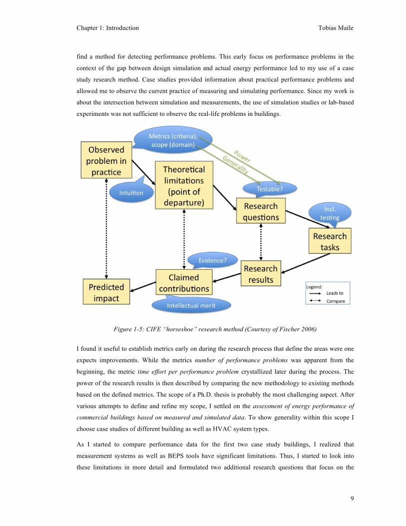
4 Research method I used the CIFE “horseshoe” research method (Fischer 2006) to guide my research. This method was
very helpful to understand all aspects of my doctoral thesis and identify areas that I needed to attend to
at each step. I will describe the aspects of the horseshoe method (Figure 1-5) in context of my research
process.
Starting with the observed problem that current performance assessment methods do not detect all
performance problems within a reasonable timeframe or at all, my intuition was that the comparison
between measured data and design BEPS simulation results can be used to assess actual building
performance more efficiently. My intuition led to an investigation of existing performance assessment
methods that use simulation, in particular calibration methods. While studying current knowledge
related to comparing measured and simulated data, I formulated first research questions that aimed to
Chapter 1: Introduction Tobias Maile
9
find a method for detecting performance problems. This early focus on performance problems in the
context of the gap between design simulation and actual energy performance led to my use of a case
study research method. Case studies provided information about practical performance problems and
allowed me to observe the current practice of measuring and simulating performance. Since my work is
about the intersection between simulation and measurements, the use of simulation studies or lab-based
experiments was not sufficient to observe the real-life problems in buildings.
Figure 1-5: CIFE “horseshoe” research method (Courtesy of Fischer 2006)
I found it useful to establish metrics early on during the research process that define the areas were one
expects improvements. While the metrics number of performance problems was apparent from the
beginning, the metric time effort per performance problem crystallized later during the process. The
power of the research results is then described by comparing the new methodology to existing methods
based on the defined metrics. The scope of a Ph.D. thesis is probably the most challenging aspect. After
various attempts to define and refine my scope, I settled on the assessment of energy performance of
commercial buildings based on measured and simulated data. To show generality within this scope I
choose case studies of different building as well as HVAC system types.
As I started to compare performance data for the first two case study buildings, I realized that
measurement systems as well as BEPS tools have significant limitations. Thus, I started to look into
these limitations in more detail and formulated two additional research questions that focus on the
Chapter 1: Introduction Tobias Maile
10
documentation of these limitations. In the context of limitations of measurement systems I assessed
existing guidelines for the measurement data set, based on the results of one case study, to illustrate
how many known performance problems can be found based on the number of sensors required by each
guideline. While progressively developing the EPCM and researching various existing processes that
could be integrated, I found that a structure is needed to organize the increasing number of measured
and simulated data points. This led me to the second research question of how to represent building
objects in a hierarchical way. Together these four questions and the process to formulate them were
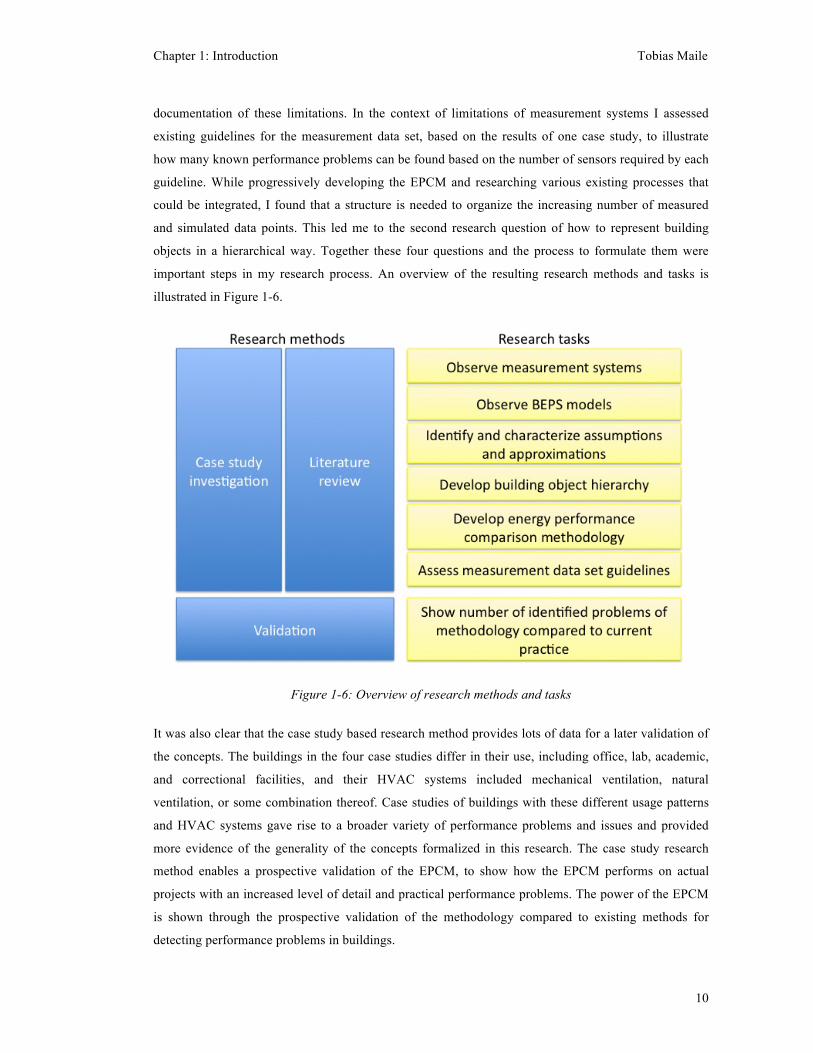
important steps in my research process. An overview of the resulting research methods and tasks is
illustrated in Figure 1-6.
Figure 1-6: Overview of research methods and tasks
It was also clear that the case study based research method provides lots of data for a later validation of
the concepts. The buildings in the four case studies differ in their use, including office, lab, academic,
and correctional facilities, and their HVAC systems included mechanical ventilation, natural
ventilation, or some combination thereof. Case studies of buildings with these different usage patterns
and HVAC systems gave rise to a broader variety of performance problems and issues and provided
more evidence of the generality of the concepts formalized in this research. The case study research
method enables a prospective validation of the EPCM, to show how the EPCM performs on actual
projects with an increased level of detail and practical performance problems. The power of the EPCM
is shown through the prospective validation of the methodology compared to existing methods for
detecting performance problems in buildings.
Chapter 1: Introduction Tobias Maile
11
The prospective validation using one case study showed that the EPCM performs better than other
comparable methods on a time per problem basis. These validation results provide support for my main
contribution, the EPCM, and indicate that the other three concepts, the building object hierarchy and the
measurement and simulation assumptions, are needed as part of the overall ECPM. At first, it was a bit
challenging to find additional evidence for each of the three sub-contributions, but further analysis of
the data gathered about the performance problems revealed evidence of these sub-contributions. It was
relatively clear to me early on what general practical impact my work should have (more efficient
performance assessment based on design goals), and information about more detailed impacts emerged
over time. One example of a detailed impact is a better understanding of the limitations of BEPS tools
(in particular EnergyPlus) for use during operations or for evaluating limitations of measurement
systems. While this description of my research path highlights the key issues, the whole process was
iterative, and often the development of more detail of a particular aspect led to the need to update and/or
adjust various other aspects, too. For example, my personal finding from early results indicated that
detail matters, which led to a reevaluation of the point of departure to find out to what extent others deal
with detail. In particular, the scope of my doctoral thesis emerged using the horseshoe method and
crystallized over time.
5 Contributions This research offers the following four contributions to knowledge:
• Energy Performance Comparison Methodology (EPCM) based on whole building design
simulation models and real life building performance measurements
• Concept of the building object hierarchy combining two perspectives (spatial and thermal) to
represent building objects in a structured form, which includes relationships between different
levels of detail of building objects
• List of measurement assumptions and a process for using them to identify performance
problems
• List of simulation assumptions, approximations, and simplifications (AAS) and a process
for using them to identify performance problems
5.1 Energy Performance Comparison Methodology The main contribution of this thesis is the EPCM. With the EPCM, I extend the prior concepts of
comparing measured and simulated data, leading to a methodology that describes relevant tasks in
sufficient detail and has the following specific characteristics: a link to design BEPS models, an
increased level of detail, and the use of a bottom-up comparison approach.
Chapter 1: Introduction Tobias Maile
12
5.1.1 Link to design BEPS models
The EPCM is specifically based on BEPS models created during design to provide a link between the
assessment and design goals. Goals defined during design are reflected in the design BEPS model and
illustrate a baseline to which the actual building performance is compared. BEPS, while considering the
whole building performance, is also able to provide enough details on the component level. While more
detailed simulation types exist such as CFD, they are not able to provide information at the overall
building level or are too resource intensive today to provide it. On the other hand, simulations or
predictions that are only focused on a specific issue (e.g., natural ventilation) do not provide
information about the overall building performance and thus do not illustrate a reasonable baseline for
comparison. In addition, statistical prediction techniques may include inefficient operation, since they
are based on measured performance data that may already contain performance problems.
5.1.2 Increased level of detail
Since the “calibration problem” is generally underdetermined, more detail rather than less detail is
needed. With the increasing availability of measurements at the component level, this move to more
detail is achievable today. Since each building is unique in its architecture, HVAC systems, usage, and
location, details that matter for some buildings may be irrelevant for the performance of other buildings.
Thus, the EPCM illustrates this move to more detail.
5.1.3 Bottom-up comparison
Typically, comparison approaches use a top-down strategy for analyzing data. Since data at the building
level may not show differences between measured and simulated data due to possible counter-effects of
multiple problems, the analysis at the building level may not indicate major problems that actually exist.
Since it is possible to measure performance at the HVAC component level, a bottom-up approach is
technically possible and feasible with the EPCM.
5.1.4 Structured and iterative process
The EPCM is a structured and iterative process. The structure is inherent from the bottom-up approach,
but it also includes an iterative part. Starting at the lowest level of detail (set points) the iterative
adjustment of the BEPS model allows the assessor to highlight performance problems at each level of
detail.
An overview of the EPCM is illustrated in Figure 1-7. The EPCM consists of three major steps and
several tasks a performance assessor needs to perform in order to assess building performance. A
detailed description of each task is contained in Chapter 2 (Maile et al. 2010). Figure 1-7 shows the
relevant data flows (with different categories) and highlights my contributions relative to this overview
Chapter 1: Introduction Tobias Maile
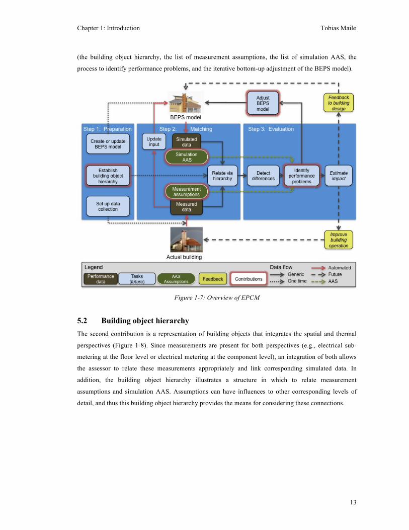
13
(the building object hierarchy, the list of measurement assumptions, the list of simulation AAS, the
process to identify performance problems, and the iterative bottom-up adjustment of the BEPS model).
Figure 1-7: Overview of EPCM
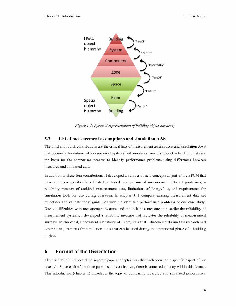
5.2 Building object hierarchy The second contribution is a representation of building objects that integrates the spatial and thermal
perspectives (Figure 1-8). Since measurements are present for both perspectives (e.g., electrical sub-
metering at the floor level or electrical metering at the component level), an integration of both allows
the assessor to relate these measurements appropriately and link corresponding simulated data. In
addition, the building object hierarchy illustrates a structure in which to relate measurement
assumptions and simulation AAS. Assumptions can have influences to other corresponding levels of
detail, and thus this building object hierarchy provides the means for considering these connections.
Chapter 1: Introduction Tobias Maile
14
Figure 1-8: Pyramid representation of building object hierarchy
5.3 List of measurement assumptions and simulation AAS The third and fourth contributions are the critical lists of measurement assumptions and simulation AAS
that document limitations of measurement systems and simulation models respectively. These lists are
the basis for the comparison process to identify performance problems using differences between
measured and simulated data.
In addition to these four contributions, I developed a number of new concepts as part of the EPCM that
have not been specifically validated or tested: comparison of measurement data set guidelines, a
reliability measure of archived measurement data, limitations of EnergyPlus, and requirements for
simulation tools for use during operation. In chapter 3, I compare existing measurement data set
guidelines and validate those guidelines with the identified performance problems of one case study.
Due to difficulties with measurement systems and the lack of a measure to describe the reliability of
measurement systems, I developed a reliability measure that indicates the reliability of measurement
systems. In chapter 4, I document limitations of EnergyPlus that I discovered during this research and
describe requirements for simulation tools that can be used during the operational phase of a building
project.
6 Format of the Dissertation The dissertation includes three separate papers (chapter 2-4) that each focus on a specific aspect of my
research. Since each of the three papers stands on its own, there is some redundancy within this format.
This introduction (chapter 1) introduces the topic of comparing measured and simulated performance
Chapter 1: Introduction Tobias Maile
15
data to identify performance problems in commercial buildings, provides details on research questions,
theoretical points of departure, and research methods, and points out my claimed contributions.
Chapter 2 details the Energy Performance Comparison Methodology and all of its tasks as well as the
building object hierarchy. It discusses existing performance assessment methods in detail and thus
provides the context for the EPCM. The prospective validation of the EPCM based on one case study is
also included in this chapter.
Chapter 3 “Formalizing measurement assumptions to document limitations of building performance
measurement systems” focuses on the measurement assumptions. It summaries measurement systems
and describes limitations of such systems based on the functions of measurement systems (sensing,
transmitting, and archiving) and illustrates how to use assumptions to document these limitations. Since
a measurement system is fundamentally bound by the set of available sensors and control points
available, it includes a review of existing guidelines to develop measurement data sets. Based on this
review and known performance problems of one case study it provides a validation of these
measurement data set guidelines. Measurement data sets and assumptions of each case study are
described in detail.
Chapter 4, “Formalizing approximations, assumptions, and simplifications to document limitations in
building energy performance simulation” focuses on simulation AAS. The chapter mentions AAS in
particular in relationship to error margins of simulation results. Descriptions of BEPS models of each
case study illustrate AAS in use. Since AAS document shortcomings of simulation models, the chapter
also provides a discussion of limitations of EnergyPlus in the context of comparing measured and
simulated data.
Both chapters 3 and 4 contain the process for identifying performance problems from differences
between measured and simulated data using measurement assumptions and simulation AAS
respectively. This process is one of the key elements within the EPCM and is thus fundamental to the
better understanding of differences between measured and simulated performance data.
The EPCM (including the building object hierarchy, measurement assumptions, and simulation AAS) is
a framework that enables an assessor to evaluate the energy performance of buildings more effectively.
Without this assessment of new energy concepts, it may be difficult to achieve the mentioned goal of
zero-net-energy commercial buildings.
7 References Augenbroe, G., and C. Park. (2005). Quantification methods of technical building performance.
Building Research & Information, 33(2), 159-172.
Austin, S.B. (1997). HVAC system trend analysis. ASHRAE Journal, 39(2), 44-50.

Chapter 1: Introduction Tobias Maile
16
Avery, G. (2002). Do averaging sensors average? ASHRAE Journal, 44(12), 42–43.
Charles, D. (2009). Leaping the Efficiency Gap. Science, 325(5942), 804-811.
Clarke, J.A. (2001). Energy simulation in building design. Oxford, UK: Butterworth-Heinemann.
Fischer, M. (2006). Formalizing Construction Knowledge for Concurrent Performance-Based Design.
Intelligent Computing in Engineering and Architecture, 4200:186-205. Berlin / Heidelberg:
Springer. http://dx.doi.org/10.1007/11888598_20 last accessed on May 12, 2010.
Gowri, K., D. Winiarski, and R. Jarnagin. (2009). Infiltration modeling guidelines for commercial
building energy analysis. PNNL #18898. Richland, WA: Pacific Northwest National
Laboratory.
Hyvarinen, J., and S. Karki. (1996). Building optimization and fault diagnosis source book. IEA Annex
#25. Espoo, Finland: International Energy Agency (IEA).
Kunz, J., T. Maile, and V. Bazjanac. (2009). Summary of the energy analysis of the first year of the
Stanford Jerry Yang & Akiko Yamazaki Environment & Energy (Y2E2) Building. Technical
Report #183. Stanford, CA: Center for Integrated Facility Engineering, Stanford University.
http://cife.stanford.edu/online.publications/TR183.pdf last accessed on March 15, 2010.
Maile, T., M. Fischer, and V. Bazjanac. (2010). A method to compare measured and simulated building
energy performance data. Working Paper #127. Stanford, CA: Center for Integrated Facility
Engineering, Stanford University.
Norman, J., H.L. MacLean, and C.A. Kennedy. (2006). Comparing High and Low Residential Density:
Life-Cycle Analysis of Energy Use and Greenhouse Gas Emissions. Journal of Urban
Planning and Development (March 2006), 132(1), 10-21.
Nyberg, M. (2002). Model-based diagnosis of an automotive engine using several types of fault models.
IEEE Transactions on control systems technology, 10(5), 679–689.
O'Donnell, J. (2009). Specification of optimum holistic building environmental and energy performance
information to support informed decision making. Ph.D. Thesis, Department of Civil and
Environmental Engineering, University College Cork (UCC), Ireland.
Persson, B. (2005). Sustainable City of Tomorrow - B0-01 - Experiences of a Swedish housing
exposition. Stockholm, Sweden: Swedish Research Council, Distributed by Coronet Books.
Piette, M.A., S. Kinney, and P. Haves. (2001). Analysis of an information monitoring and diagnostic
system to improve building operations. Energy and Buildings, 33(8), 783-791.
Reddy, T. (2006). Literature review on calibration of building energy simulation programs: Uses,
problems, procedures, uncertainty, and tools. ASHRAE Transactions, 112(1), 226-240.

Chapter 1: Introduction Tobias Maile
17
Reddy, T., J. Haberl, and J. Elleson. (1999). Engineering uncertainty analysis in the evaluation of
energy and cost savings of cooling system alternatives based on field-monitored data.
Proceedings of the ASHRAE Transactions, 105, 1047-1057. Seattle, WA: American Society of
Heating, Refrigerating and Air-Conditioning Engineers (ASHRAE).
Salsbury, T., and R. Diamond. (2000). Performance validation and energy analysis of HVAC systems
using simulation. Energy & Buildings, 32(1), 5–17.
Schmid, S., T. Lutz, and E. Krämer. (2007). Simulation of the unsteady cavity flow of the stratospheric
observatory for infrared astronomy. Proceedings of the IUTAM Symposium on Unsteady Flows
and their Control, Corfu, Greece, 14. Corfu, Greece.
Scofield, J.H. (2002). Early performance of a green academic building. ASHRAE Transactions, 108(2),
1214–1232.
Seidl, R. (2006). Trend analysis for commissioning. ASHRAE Journal, 48(1), 34-43.
Sissine, F. (2007). Energy Independence and Security Act of 2007: A summary of major provisions.
Congressional Report #475228. Washington, DC: Congressional Research Service.
http://oai.dtic.mil/oai/oai?verb=getRecord&metadataPrefix=html&identifier=ADA475228 last
accessed on July 8, 2010.
Sun, J., and T. Reedy. (2006). Calibration of Building Energy Simulation Programs using the
Analytic Optimization Approach. HVAC&R Research Journal, 12(1), 177-196.
Wang, F., H. Yoishida, S. Masuhara, H. Kitagawa, and K. Goto. (2005). Simulation-based automated
commissioning method for air-conditioning systems and its application case study.
Proceedings of the 9th IBPSA conference. Montreal, Canada: International Building
Performance Simulation Association.
Walsh, B., B. Urban, and S. Herkel. (2009). Innovating for better buildings - An opportunity disguised
as a meltdown. Technical report. San Francisco, CA: Nth Power.
http://www.nthpower.com/newsletter/InnovatingBetterBuildings_FINAL.pdf last accessed on
August 17, 2009.
Xu, P., P. Haves, and M. Kim. (2005). Model-based automated functional testing-methodology and
application to air handling units. ASHRAE Transactions, 111(1), 979-989.
Chapter 2: EPCM Tobias Maile
18
Chapter 2: A method to compare measured and simulated
data to assess building energy performance
Tobias Maile, Martin Fischer, Vladimir Bazjanac
1 Abstract Building energy performance is often inadequate given design goals. While different types of
assessment methods exist, they either do not consider design goals and/or are not flexible enough to
integrate new and innovative energy concepts. However, innovative energy concepts are needed to
comply with new regulations that aim to decrease energy use in buildings. One reason for the missing
flexibility of assessment methods is their development and testing based on one single case study,
which makes them very specific and less flexible. Furthermore, existing assessment methods focus
mostly on the building and system level while ignoring more detailed data. With the availability and
affordability of more detailed measured data, a more detailed performance assessment is possible.
However, the increased number of measured data points requires a structure to organize these data.
Existing representations of building objects that would structure measured data typically focus on a
single perspective and lack relationships between building objects that are present in buildings and that
are needed to understand the interplay within heating, ventilation and air conditioning (HVAC) systems
and assess their performance. This paper presents the Energy Performance Comparison Methodology
(EPCM), which enables the identification of performance problems based on a comparison of measured
performance data and simulated performance data representing design goals. The EPCM is based on an
interlinked building object hierarchy that includes necessary relationships among building objects by
integrating the spatial and thermal perspectives. We focus on the process of comparing performance
data from the bottom up, starting with control set points and leading to total building performance data.
This research is based on multiple case studies that provide real-life context for performance problems
and measured and simulated performance data. We also prospectively validated the EPCM and the
building object hierarchy with an additional case study.
2 Introduction Building energy performance problems are a well-known issue (Mills et al. 2005). Several studies show
that heating, ventilation and air conditioning (HVAC) systems in buildings do not operate as predicted
during design because of performance problems (Scofield 2002; Piette et al. 2001; Persson 2005; Kunz
et al. 2009). These studies indicate an untapped potential to reduce energy consumption of buildings
Chapter 2: EPCM Tobias Maile
19
and highlight the gap between design and actual energy performance. In addition to these studies, new
regulations aim to decrease energy consumption in buildings (e.g., Sissine 2007) and thus further
increase the need to close the gap between design goals and actual energy performance of buildings.
Existing methods that compare measured and simulated data focus on the building and/or system level.
When this focus is used, modeling inaccuracies can be hidden through compensation errors (Clarke
2001). Existing comparison approaches (e.g., Salsbury and Diamond 2000) describe the comparison in
a generic fashion and do not include details about processes or tasks. Automated performance
assessment methods focus on the component level or on specific types of systems (e.g., Xu et al. 2005).
To assess the energy performance of all levels of detail in a building a comparison that ranges from the
component to the building level and a systematic methodology are needed. Due to an increased number
of data available, a hierarchy is needed that allows to relate different data streams to each other and sets
them into context of the building and its HVAC systems. Examples of related data streams are space
level and system level water temperatures that greatly depend on each other. Since measured
performance data are linked to HVAC systems and components but also to spatial objects, a
representation that combines both perspectives is necessary. The first building object hierarchy that
considers the spatial and thermal perspective focuses on zone components (O'Donnell 2009) and does
not include topological relationships as well as relationships between HVAC components of different
HVAC systems. Since performance data are tied to spatial and HVAC components, a hierarchy is
needed that combine both perspectives and that describe the relationships to neighboring as well as
parent objects.
We developed the Energy Performance Comparison Methodology (EPCM), which supports
identification of performance problems based on comparison of measured and simulated data. This
method incorporates design goals by using building performance energy simulation (BEPS) models
generated during design and provides an assessment of the actual building’s performance compared to
the performance simulated with design BEPS models. The BEPS models provide a benchmark for
comparison of the actual performance. The benchmark includes design goals, which are otherwise often
neglected during operation, and is a useful reference to understand the anticipated performance of the
building. The EPCM was developed based on the experience of comparing measured and simulated
data in two case studies. It was prospectively validated on an additional case study. This methodology
builds on and extends three areas: measuring building energy performance, simulating building energy
performance, and comparing the resulting measured and simulated data. Data acquisition systems
archive the measured data for use by the EPCM. Detailed whole-building energy performance
simulation tools such as EnergyPlus produce the simulated data for this comparison. This paper
describes the EPCM in detail, including the formal representation of building objects in the form of a
building object hierarchy that captures additional relationships of objects compared to existing
hierarchies. Other critical aspects of the EPCM are the identification and appropriate consideration of

Chapter 2: EPCM Tobias Maile
20
measurement assumptions and simulation approximations, assumptions, and simplifications (AAS).
Measurement assumptions document limitations of measurement systems while simulation AAS
document limitations of BEPS models. The documentation of both types of limitations is needed to
evaluate difference between measured and simulated data. In particular, these limitations can hinder a
matching of measured and simulated data and thus need to be considered when comparing performance
data. Maile et al. (2010b) discuss measurement assumptions and their use to understand limitations of
measurement systems. Maile et al. (2010a) describe simulation AAS and their use to understand
limitations of building energy performance simulation data. Within the EPCM, both the measurement
assumptions and simulation AAS are analyzed to identify performance problems based on differences
between measured and simulated data. During the assessment process the BEPS model is adjusted so
that simulation results match more closely with the actual performance of the building.
Due to the increased level of detail and the goal of the EPCM to identify actual performance problems,
we base our research on case studies to provide real-life context (Yin 2003) for performance problems
in buildings. We elaborate on the development of the EPCM (section 3) and provide a discussion of
existing performance assessment methods and highlight the shortcomings of existing methods (section
3.4). We describe the EPCM in detail (section 4). Results from applying the EPCM on a case study
(section 5) and details about our validation of the formal representation and the methodology itself are
shown (section 6). Through the validation, we show the generality of EPCM through different case
study building usage and HVAC systems and the power of EPCM compared to standard practice.
Lastly, we describe limitations and possible future research areas (section 7).
3 Development of the EPCM We developed the EPCM based on two initial case studies and one validation case studies. We discuss
the need for the case study research method and detail our selection of case studies. We illustrate early
comparisons and their effect on the development of the EPCM as well as describe existing assessment
methods in detail.
3.1 Research method: case studies Since our main focus and goal of the EPCM is to identify performance problems in buildings, we
needed a research method that allows the observation of performance problems in practice. In addition,
the level of detail plays an important role in this research. Both criteria led to the selection of a case
study based research method. Case studies are the typical research method in this field, with most
researchers using a single case study. The problem with single case studies is the lack of generality of
the resulting methods. Survey or interview methods are not applicable due to the lack of knowledge and
standard practice that would be necessary for them. From a research validation perspective, it was also
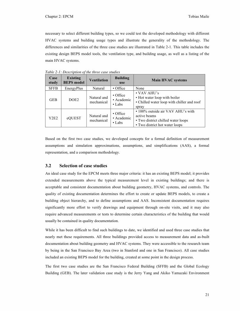
Chapter 2: EPCM Tobias Maile
21
necessary to select different building types, so we could test the developed methodology with different
HVAC systems and building usage types and illustrate the generality of the methodology. The
differences and similarities of the three case studies are illustrated in Table 2-1. This table includes the
existing design BEPS model tools, the ventilation type, and building usage, as well as a listing of the
main HVAC systems.
Table 2-1: Description of the three case studies Case study
Existing BEPS model Ventilation Building
use Main HVAC systems
SFFB EnergyPlus Natural • Office None
GEB DOE2 Natural and mechanical
• Office • Academic • Labs
• VAV AHU’s • Hot water loop with boiler • Chilled water loop with chiller and roof spray
Y2E2 eQUEST Natural and mechanical
• Office • Academic • Labs
• 100% outside air VAV AHU’s with active beams • Two district chilled water loops • Two district hot water loops
Based on the first two case studies, we developed concepts for a formal definition of measurement
assumptions and simulation approximations, assumptions, and simplifications (AAS), a formal
representation, and a comparison methodology.
3.2 Selection of case studies An ideal case study for the EPCM meets three major criteria: it has an existing BEPS model; it provides
extended measurements above the typical measurement level in existing buildings; and there is
acceptable and consistent documentation about building geometry, HVAC systems, and controls. The
quality of existing documentation determines the effort to create or update BEPS models, to create a
building object hierarchy, and to define assumptions and AAS. Inconsistent documentation requires
significantly more effort to verify drawings and equipment through on-site visits, and it may also
require advanced measurements or tests to determine certain characteristics of the building that would
usually be contained in quality documentation.
While it has been difficult to find such buildings to date, we identified and used three case studies that
nearly met these requirements. All three buildings provided access to measurement data and as-built
documentation about building geometry and HVAC systems. They were accessible to the research team
by being in the San Francisco Bay Area (two in Stanford and one in San Francisco). All case studies
included an existing BEPS model for the building, created at some point in the design process.
The first two case studies are the San Francisco Federal Building (SFFB) and the Global Ecology
Building (GEB). The later validation case study is the Jerry Yang and Akiko Yamazaki Environment

Chapter 2: EPCM Tobias Maile
22
and Energy Building (Y2E2) at Stanford. These case studies include one office building (SFFB), two
mixed-use research and office buildings (GEB and Y2E2). The observed portion of SFFB has a natural
ventilation system. GEB and Y2E2 have a mixture between natural and mechanical ventilation systems.
3.3 Early comparisons The SFFB case study was our first case study, and thus it initiated early concepts around the EPCM. In
particular, it was apparent from early comparison graphs that more knowledge was necessary to
understand the meaning of specific comparisons of measured and simulated data. For example, Figure
2-1 illustrates two early comparison graphs. The left graph shows that the simulated space temperature
did not match with the measured counterparts at 100% airflow. However, the right graph shows a
reasonable match between measured and simulated space temperatures at 25% of airflow. The
difference between the measured and simulated airflow can be explained with two assumptions. The
first simulation assumption is that the bulk airflow in the BEPS model cannot capture all dynamic
effects of the actual airflow. The second measurement assumption is that the velocity measurements are
spot measurements and thus do not directly correlate with the average airflow over the opening area in
the simulation model. These insights lead to the development of the EPCM and the concepts of
measurement assumption (Maile et al. 2010b) and simulation AAS (Maile et al. 2010a).
Figure 2-1: Example comparison graphs from SFFB
(left – Space air temperature comparison based on 100% airflow; right – Space air temperature
comparison based on 25% airflow)
3.4 Existing methods to detect performance problems Figure 2-2 shows existing methods for detecting performance problems in buildings on two dimensions:
life-cycle phases and level of detail. Traditional commissioning tests the functioning of a HVAC
component (Grob and Madjidi 1997). However, correctly operating HVAC components do not ensure
efficient operation on the system and building levels. Furthermore, the increasing complexity of HVAC
systems increases the difficulty of testing the proper functionality of HVAC systems. Another technique
used during the commissioning is trend analysis (e.g., Austin 1997; Seidl 2006), which focuses on

Chapter 2: EPCM Tobias Maile
23
detecting performance problems by analyzing measured data. To address the problem of manual and
time-consuming commissioning, several automated commissioning methods have been developed. For
example, Wang et al. (2005) describe an automated commissioning method for a specific air
conditioning system based on a simulation model that was specifically developed for that purpose. Xu
et al. (2005) use a similar simulation model approach, but base their analysis on functional tests that
require interference with the actual operation of the building. These methods use simulation models that
are used only during commissioning and thus are not linked to design. These automated methods are
limited to known and typical HVAC system configurations and require additional development for new
or innovative configurations or HVAC components.
Figure 2-2: Overview of existing performance comparison methods
Traditionally, building operation is based on feedback from occupants. Building operators address
issues on the basis of complaints and usually adjust local set points instead of troubleshooting the
problem and resolving it (Katipamula et al. 2003). Thus, this approach focuses mostly on the space
level, based on occupant complaints.
There are also a number of commercially available tools (e.g., Santos and Rutt 2001) that provide rule-
based automated fault detection. Their focus is mainly on the system level. The disadvantage of those
tools is the large installation effort and the predefined set of rules. Due to the need for predefined rules,
new innovative HVAC systems and HVAC components cannot be evaluated with rule-based fault
detection.
Chapter 2: EPCM Tobias Maile
24
Last but not least, calibrated simulation models are often used to establish a baseline simulation model
for comparison to possible retrofit measures. Calibrated simulation models are also used to verify the
performance of HVAC systems, mostly on building and system levels. The problem with simulation
model calibration is that compensating errors can mask modeling inaccuracies at the whole building
level (Clarke 2001). As a result, problems in the building may not be identified due to the dynamic
relationships among different parts of a building. Thus “calibration” is necessary on a component level
to circumvent the compensation errors. A simulation model is often labeled as “calibrated” if it falls
within a specific error margin (e.g., 5%). This results in a trial-and-error approach of changing input
parameters until the result is within the specified error margin. That is why multiple “solutions” (input
data configurations) are possible; thus, the selection of one possible solution is arbitrary (Reddy 2006).
Commissioning methods and calibrated simulation models typically describe a one-time event rather
than an ongoing process for continuously controlling the performance of buildings. Several studies
(Cho 2002; Frank et al. 2007) show that building performance decreases after one-time improvements.
Therefore, we recommend data archiving and analysis over the complete life of a building.
All of these methods (except calibrated simulation models) fail to provide a link to design building
energy performance simulation (BEPS). Thus, there is a gap between design BEPS and existing
performance assessment methods. There are two main reasons why the link to design BEPS models is
important. Design BEPS models contain the design goals, and thus these models should be the basis for
an assessment to determine whether the completed product complies with the design goals. The second
reason is to provide feedback to building design and the design BEPS model. Results of design BEPS
models typically do not match with actual performance (e.g., Scofield 2002; Piette et al. 2001), thus a
detailed method to detect differences between measured and simulated data is needed.
4 Energy Performance Comparison Methodology (EPCM) The goal of the EPCM is to provide feedback to building design and operation. This feedback is based
on performance problems and the subsequent estimation of their impact on thermal comfort and energy
consumption. In this paper we focus on the tasks of the EPCM up until the identification of
performance problems.
We call the person performing the tasks of the EPCM the performance assessor. Because such an
assessment of actual building energy performance compared to design goals is rather rare in practice,
we chose a new description for that person, who can be a HVAC design engineer with background in
measuring, simulating, and/or commissioning.
The EPCM steps (the preparation, matching, and evaluation steps) and tasks are based on the flow of
data (Figure 2-3). Step 1, the preparation step, includes tasks that create or update the BEPS model, set
up data collection, and establish a building object hierarchy. All tasks in the preparation step are
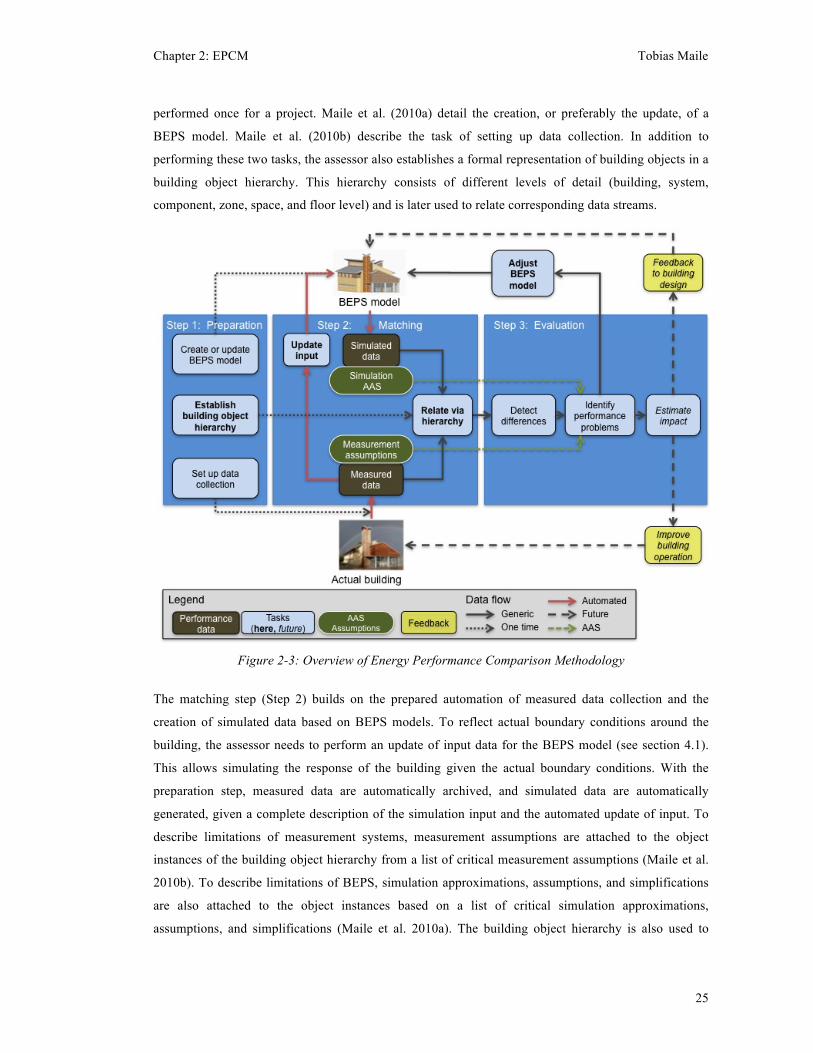
Chapter 2: EPCM Tobias Maile
25
performed once for a project. Maile et al. (2010a) detail the creation, or preferably the update, of a
BEPS model. Maile et al. (2010b) describe the task of setting up data collection. In addition to
performing these two tasks, the assessor also establishes a formal representation of building objects in a
building object hierarchy. This hierarchy consists of different levels of detail (building, system,
component, zone, space, and floor level) and is later used to relate corresponding data streams.
Figure 2-3: Overview of Energy Performance Comparison Methodology
The matching step (Step 2) builds on the prepared automation of measured data collection and the
creation of simulated data based on BEPS models. To reflect actual boundary conditions around the
building, the assessor needs to perform an update of input data for the BEPS model (see section 4.1).
This allows simulating the response of the building given the actual boundary conditions. With the
preparation step, measured data are automatically archived, and simulated data are automatically
generated, given a complete description of the simulation input and the automated update of input. To
describe limitations of measurement systems, measurement assumptions are attached to the object
instances of the building object hierarchy from a list of critical measurement assumptions (Maile et al.
2010b). To describe limitations of BEPS, simulation approximations, assumptions, and simplifications
are also attached to the object instances based on a list of critical simulation approximations,
assumptions, and simplifications (Maile et al. 2010a). The building object hierarchy is also used to
Chapter 2: EPCM Tobias Maile
26
relate measured and simulated data streams into data pairs (section 4.2). An example of a data pair is a
measured space temperature and its corresponding simulated space temperature for a specific space in
the building.
In the assessment step, the assessor identifies differences between the members of the above mentioned
data pairs, on both a visual and a statistical basis (section 4.3). Based on these differences, the assessor
identifies performance problems with the help of measurement assumptions and simulation
approximations, assumptions, and simplifications (section 4.3). Based on the identified performance
problems, the assessor performs an iterative process (section 4.4) of adjusting input data of the BEPS
model to eliminate incorrect design AAS to improve the matching of measured and simulated data.
Since the actual building operation and measured data cannot be changed retrospectively, this iterative
process focuses on simulated data. For each specific time frame under observation, the BEPS model is
adjusted to eliminate AAS and incorporate changes of the actual building compared to the design BEPS
model, to match measured and simulated data more closely. Since the actual building is a dynamic
environment, changes to the building typically occur. In particular, changes to the control strategy or
changes to the usage of the building or changes to the geometry are important for the use of EPCM.
This is why we introduce events that describe these changes to the building and define time frames for
investigation within the EPCM.
4.1 Updating simulation input This section describes how to update simulation input data with measured data. For a meaningful
comparison of measured and simulated data, it is important to define accurate boundary conditions,
typically residing in a weather file, around a given building. While outside weather data are obvious
boundary conditions, simulation input can also consist of other additional measurements. These other
measurements include occupancy, plug loads, electric lighting, and others. In addition, input for the
simulation may include space temperature set points, particularly if those are user-adjustable.
The initial update includes external boundary conditions, which are outside air temperature, solar
radiation (separate direct and diffuse radiation measurements are preferred), wind speed and direction,
as well as wet bulb temperature or relative humidity (whichever is available). Throughout the iterations
of the EPCM, more measurement data are used as input for the simulation. If available, the set of input
updates includes space temperature set points and measurements related to internal loads. While space
temperature set points are most likely available on a zone respective space level, internal load
measurements are typically not available at this granularity. If the measurement data are less detailed
than the simulation data (e.g., floor-based measurements, but a space-based BEPS model), the assessor
needs to convert the measurement from floors to spaces (floor area to space area) and assign different
weights depending on space types.
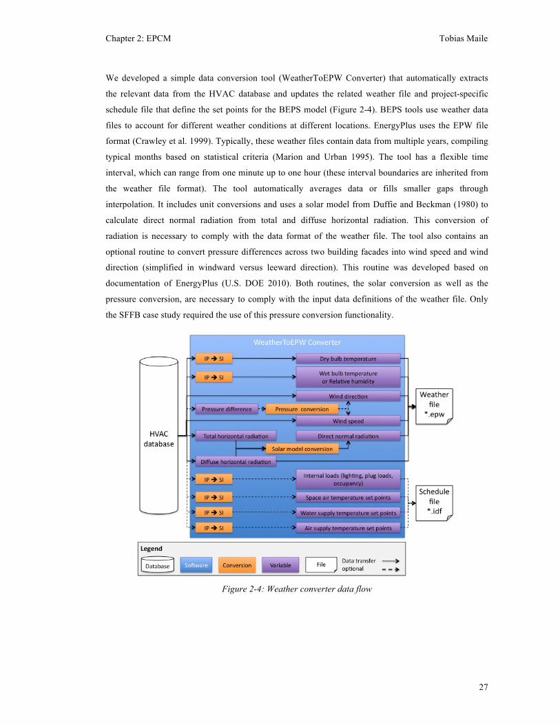
Chapter 2: EPCM Tobias Maile
27
We developed a simple data conversion tool (WeatherToEPW Converter) that automatically extracts
the relevant data from the HVAC database and updates the related weather file and project-specific
schedule file that define the set points for the BEPS model (Figure 2-4). BEPS tools use weather data
files to account for different weather conditions at different locations. EnergyPlus uses the EPW file
format (Crawley et al. 1999). Typically, these weather files contain data from multiple years, compiling
typical months based on statistical criteria (Marion and Urban 1995). The tool has a flexible time
interval, which can range from one minute up to one hour (these interval boundaries are inherited from
the weather file format). The tool automatically averages data or fills smaller gaps through
interpolation. It includes unit conversions and uses a solar model from Duffie and Beckman (1980) to
calculate direct normal radiation from total and diffuse horizontal radiation. This conversion of
radiation is necessary to comply with the data format of the weather file. The tool also contains an
optional routine to convert pressure differences across two building facades into wind speed and wind
direction (simplified in windward versus leeward direction). This routine was developed based on
documentation of EnergyPlus (U.S. DOE 2010). Both routines, the solar conversion as well as the
pressure conversion, are necessary to comply with the input data definitions of the weather file. Only
the SFFB case study required the use of this pressure conversion functionality.
Figure 2-4: Weather converter data flow

Chapter 2: EPCM Tobias Maile
28
4.2 Building object hierarchy Due to the large number of data points (e.g., 2,231 data points at Y2E2), a formal representation is
needed that allows organizing these data points. Such a representation needs to link building objects so
that reasoning about differences between measured and simulated data of related building objects
becomes possible. While various approaches exist for defining a building object hierarchy, almost all
focus on only one perspective. Most common is a thermal perspective hierarchy, consisting of HVAC
system, sub-system, and HVAC component levels (Husaunndee et al. 1997; Bazjanac and Maile 2004;
Visier et al. 2004). Another common representation is a spatial perspective that includes building, floor,
and zone/space levels. O'Donnell (2009) combines both perspectives into one tree structure that is
focused on the zone object. The relevant HVAC hierarchy is connected to each zone, which leads to
duplicate instances of HVAC systems and components and does not account for relationships among
components of different HVAC systems. Furthermore, O’Donnell’s representation lacks a space object.
Interval Data Systems (IDS 2004) discuss the usefulness of various perspectives to building objects
such as facility, organizational, or HVAC system hierarchies. However, they do not mention the
relationships among different viewpoints.
A BEPS model typically contains some of these relationships between building objects. In EnergyPlus,
each zone is part of the building and indirectly linked to neighboring zones through connected surfaces
objects. The concept of a floor, i.e., an agglomeration of spaces, is missing in EnergyPlus. However, the
HVAC components are part of a specific HVAC system and are organized in branches that connect the
HVAC components including the flow direction. In addition, the HVAC components on the zone level
are linked to the related zone objects.
Measured and simulated data points represent different objects on different levels of detail in a building.
Due to increasing numbers of available sensors in buildings, the current focus on HVAC systems and
HVAC hierarchies does not capture the interconnections between HVAC and spatial objects. Thus, we
define a hierarchy that contains both spatial and thermal perspectives (Figure 2-5).
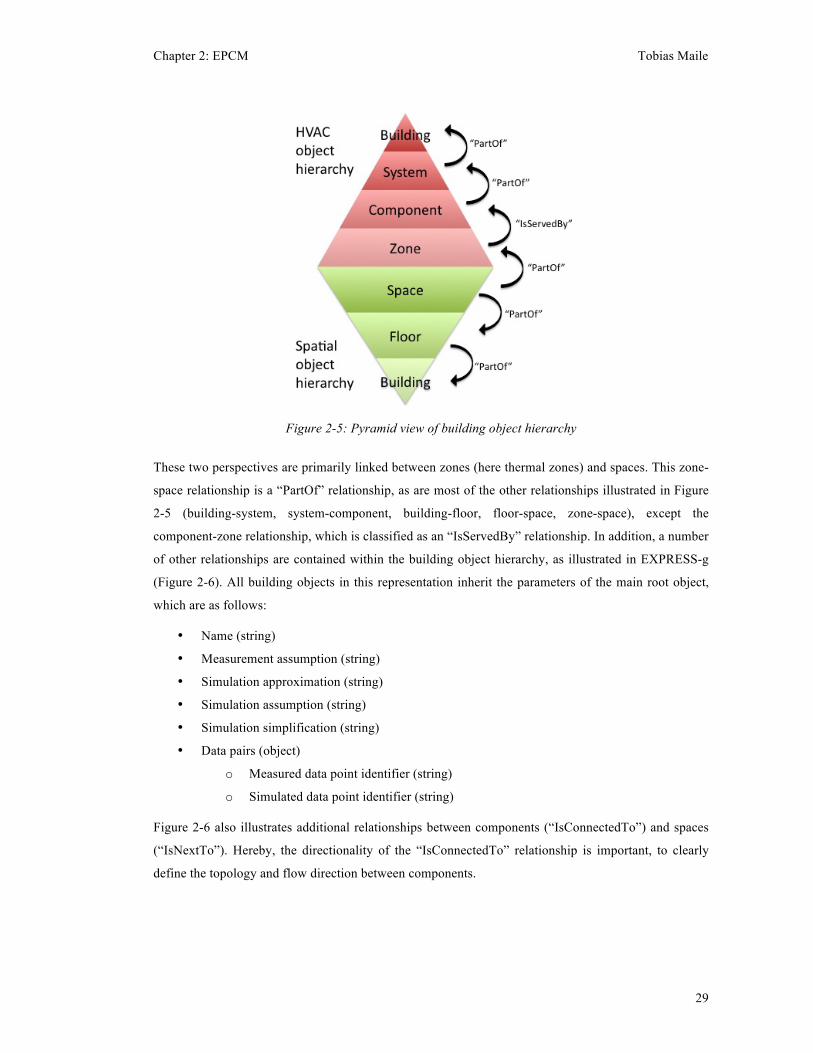
Chapter 2: EPCM Tobias Maile
29
Figure 2-5: Pyramid view of building object hierarchy
These two perspectives are primarily linked between zones (here thermal zones) and spaces. This zone-
space relationship is a “PartOf” relationship, as are most of the other relationships illustrated in Figure
2-5 (building-system, system-component, building-floor, floor-space, zone-space), except the
component-zone relationship, which is classified as an “IsServedBy” relationship. In addition, a number
of other relationships are contained within the building object hierarchy, as illustrated in EXPRESS-g
(Figure 2-6). All building objects in this representation inherit the parameters of the main root object,
which are as follows:
• Name (string)
• Measurement assumption (string)
• Simulation approximation (string)
• Simulation assumption (string)
• Simulation simplification (string)
• Data pairs (object)
o Measured data point identifier (string)
o Simulated data point identifier (string)
Figure 2-6 also illustrates additional relationships between components (“IsConnectedTo”) and spaces
(“IsNextTo”). Hereby, the directionality of the “IsConnectedTo” relationship is important, to clearly
define the topology and flow direction between components.
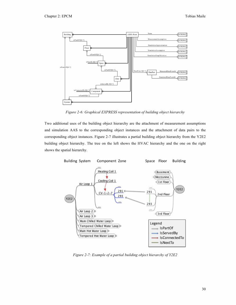
Chapter 2: EPCM Tobias Maile
30
Figure 2-6: Graphical EXPRESS representation of building object hierarchy
Two additional uses of the building object hierarchy are the attachment of measurement assumptions
and simulation AAS to the corresponding object instances and the attachment of data pairs to the
corresponding object instances. Figure 2-7 illustrates a partial building object hierarchy from the Y2E2
building object hierarchy. The tree on the left shows the HVAC hierarchy and the one on the right
shows the spatial hierarchy.
Figure 2-7: Example of a partial building object hierarchy of Y2E2

Chapter 2: EPCM Tobias Maile
31
Due to simulation AAS, the building object hierarchy of the BEPS model may be slightly different
(missing components, simplifications, workarounds, etc.) than that of the actual building. In the context
of the EPCM, the building object hierarchy is always based on the actual building, since measurements
are based on the actual building. Simulation AAS assigned to the building object hierarchy describe the
simulation simplifications and allow circumventing this issue of different hierarchical representations of
the actual building and the BEPS model.
Figure 2-8 shows an example that illustrates the use of the building object hierarchy. Airflow on the
system and component level correlates during occupied hours but is different during unoccupied hours.
While it is not clear where the difference originates by only considering the system level, by
considering the component level it becomes clear that there is a relationship between the two
differences due to similar characteristics. However, the origin is still unclear without the knowledge of
the simulation simplification on the space level that the active chilled beam model is single speed
(compared to two speed). Thus the airflow at the lower speed is zero in the model and causes the
difference in both graphs. The relationships of the building object hierarchy enable such a reasoning,
which would be rather difficult if not impossible without it.
Figure 2-8: Example comparison of airflow on the system (left) and component (right) level
(during occupied hours (grey) measured and simulated data match reasonably close while during
unoccupied hours there is a difference between measured and simulated data on the system and
component level)
4.3 Process of identifying performance problems with the knowledge of
measurement assumptions and simulation AAS Limitations of measurement systems in buildings as well as limitations of BEPS models are the reasons
that specific data points in a building may not match simulation results. Measurement assumptions
describe limitations of measurement systems (Maile et al. 2010a) and simulation AAS describe
limitations of BEPS models (Maile et al. 2010b). We use measurement assumptions and simulation
AAS to identify performance problems from differences between measured and simulated data as
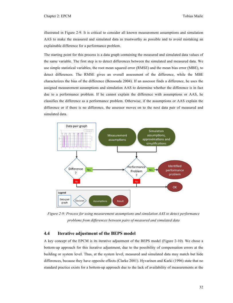
Chapter 2: EPCM Tobias Maile
32
illustrated in Figure 2-9. It is critical to consider all known measurement assumptions and simulation
AAS to make the measured and simulated data as trustworthy as possible and to avoid mistaking an
explainable difference for a performance problem.
The starting point for this process is a data graph containing the measured and simulated data values of
the same variable. The first step is to detect differences between the simulated and measured data. We
use simple statistical variables, the root mean squared error (RMSE) and the mean bias error (MBE), to
detect differences. The RMSE gives an overall assessment of the difference, while the MBE
characterizes the bias of the difference (Bensouda 2004). If an assessor finds a difference, he uses the
assigned measurement assumptions and simulation AAS to determine whether the difference is in fact
due to a performance problem. If he cannot explain the difference with assumptions or AAS, he
classifies the difference as a performance problem. Otherwise, if the assumptions or AAS explain the
difference or if there is no difference, the assessor moves on to the next data pair of measured and
simulated data.
Figure 2-9: Process for using measurement assumptions and simulation AAS to detect performance
problems from differences between pairs of measured and simulated data
4.4 Iterative adjustment of the BEPS model A key concept of the EPCM is its iterative adjustment of the BEPS model (Figure 2-10). We chose a
bottom-up approach for this iterative adjustment, due to the possibility of compensation errors at the
building or system level. Thus, at the system level, measured and simulated data may match but hide
differences, because they have opposite effects (Clarke 2001). Hyvarinen and Karki (1996) state that no
standard practice exists for a bottom-up approach due to the lack of availability of measurements at the
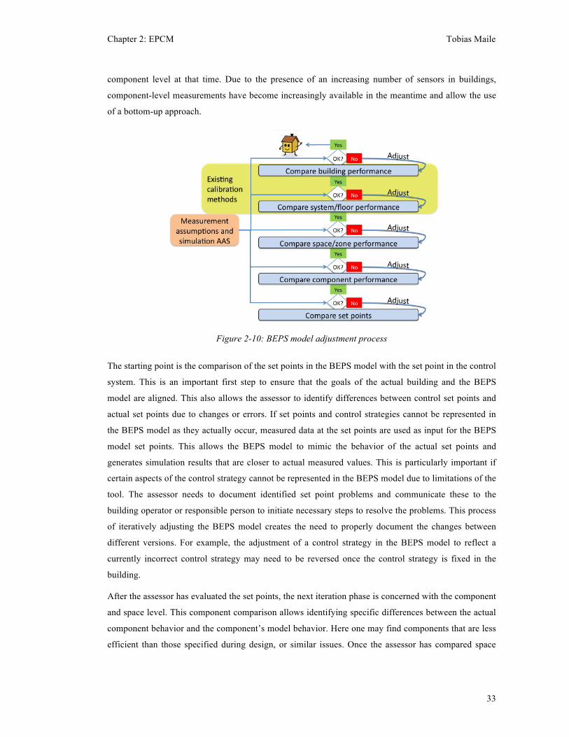
Chapter 2: EPCM Tobias Maile
33
component level at that time. Due to the presence of an increasing number of sensors in buildings,
component-level measurements have become increasingly available in the meantime and allow the use
of a bottom-up approach.
Figure 2-10: BEPS model adjustment process
The starting point is the comparison of the set points in the BEPS model with the set point in the control
system. This is an important first step to ensure that the goals of the actual building and the BEPS
model are aligned. This also allows the assessor to identify differences between control set points and
actual set points due to changes or errors. If set points and control strategies cannot be represented in
the BEPS model as they actually occur, measured data at the set points are used as input for the BEPS
model set points. This allows the BEPS model to mimic the behavior of the actual set points and
generates simulation results that are closer to actual measured values. This is particularly important if
certain aspects of the control strategy cannot be represented in the BEPS model due to limitations of the
tool. The assessor needs to document identified set point problems and communicate these to the
building operator or responsible person to initiate necessary steps to resolve the problems. This process
of iteratively adjusting the BEPS model creates the need to properly document the changes between
different versions. For example, the adjustment of a control strategy in the BEPS model to reflect a
currently incorrect control strategy may need to be reversed once the control strategy is fixed in the
building.
After the assessor has evaluated the set points, the next iteration phase is concerned with the component
and space level. This component comparison allows identifying specific differences between the actual
component behavior and the component’s model behavior. Here one may find components that are less
efficient than those specified during design, or similar issues. Once the assessor has compared space

Chapter 2: EPCM Tobias Maile
34
and component performance the next step is to look at system performance. Here the focus is on
system-specific variables and the energy consumption of systems. Lastly, the comparison is done on the
building level. Existing simulation model calibration methods typically compare only at the building
and system levels and are highlighted for comparison in Figure 2-10.
A technique to simplify and decrease the simulation time is to use partial BESP models during the
adjustment process. Encapsulating a specific part of the BEPS model while providing measured data as
boundary conditions for that specific part enables a more detailed analysis of a specific aspect of the
BEPS model. For example, to investigate a specific space in further detail neighboring space conditions
can be overwritten by the measured conditions; thus the assessor can focus on analyzing that particular
space without the effects of neighboring spaces.
Another important factor for evaluating building energy performance data are events. While events
related to atypical occupancy (such as events with increased occupancy or decreased occupancy) can
easily be integrated into a BEPS model, changes in the geometry, the HVAC system or the controls of
the building may require a different version of the BEPS model. The importance of these events is
twofold, reflected by atypical schedule events and change events. Atypical schedule events, such as
occupancy changes, can be reflected in occupancy schedules. Change events, including control, HVAC
system, and geometry changes, typically require the use of a different version of a BEPS model. For
example, it may not be possible to implement two substantially different control strategies within the
same BEPS model. Geometry change events due to remodeling efforts require the use of different
versions of the BEPS model. An example from Y2E2 is a lab area in the basement that was remodeled
to be a multiuse space with offices integrated into the lab area. The documentation of these events is
important to clarify the use of different versions of BEPS models.
Table 2-2: Examples of events at Y2E2
Event Start (date and time)
End (date and time)
Object level Consequences
Building shutdown June 26 2008 6:00 PM
June 27 2008 6: 00 AM Building
No data during shutdown; data around shutdown may show unconventional values
Natural ventilation control strategy change #3
October 11 2009 3:00 PM
Permanent change Atria Improvement of control
strategy
Construction in lab area
January 13 2008 6:00 AM
July 26 2008 4:00 PM
Space B27
Geometry change, HVAC changes and construction activity
Student orientation week
September 26 2009
September 28 2009 Building Unusually high occupancy at
red atrium
These events are linked to the building object hierarchy on the corresponding building object level to
allow a proper assignment to the related aspect of the BEPS model. Design BEPS tools do not provide
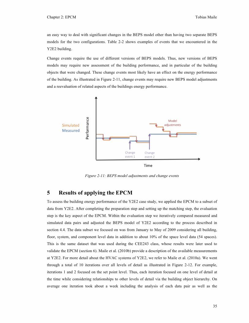
Chapter 2: EPCM Tobias Maile
35
an easy way to deal with significant changes in the BEPS model other than having two separate BEPS
models for the two configurations. Table 2-2 shows examples of events that we encountered in the
Y2E2 building.
Change events require the use of different versions of BEPS models. Thus, new versions of BEPS
models may require new assessment of the building performance, and in particular of the building
objects that were changed. These change events most likely have an effect on the energy performance
of the building. As illustrated in Figure 2-11, change events may require new BEPS model adjustments
and a reevaluation of related aspects of the buildings energy performance.
Figure 2-11: BEPS model adjustments and change events
5 Results of applying the EPCM To assess the building energy performance of the Y2E2 case study, we applied the EPCM to a subset of
data from Y2E2. After completing the preparation step and setting up the matching step, the evaluation
step is the key aspect of the EPCM. Within the evaluation step we iteratively compared measured and
simulated data pairs and adjusted the BEPS model of Y2E2 according to the process described in
section 4.4. The data subset we focused on was from January to May of 2009 considering all building,
floor, system, and component level data in addition to about 10% of the space level data (54 spaces).
This is the same dataset that was used during the CEE243 class, whose results were later used to
validate the EPCM (section 6). Maile et al. (2010b) provide a description of the available measurements
at Y2E2. For more detail about the HVAC systems of Y2E2, we refer to Maile et al. (2010a). We went
through a total of 10 iterations over all levels of detail as illustrated in Figure 2-12. For example,
iterations 1 and 2 focused on the set point level. Thus, each iteration focused on one level of detail at
the time while considering relationships to other levels of detail via the building object hierarchy. On
average one iteration took about a week including the analysis of each data pair as well as the
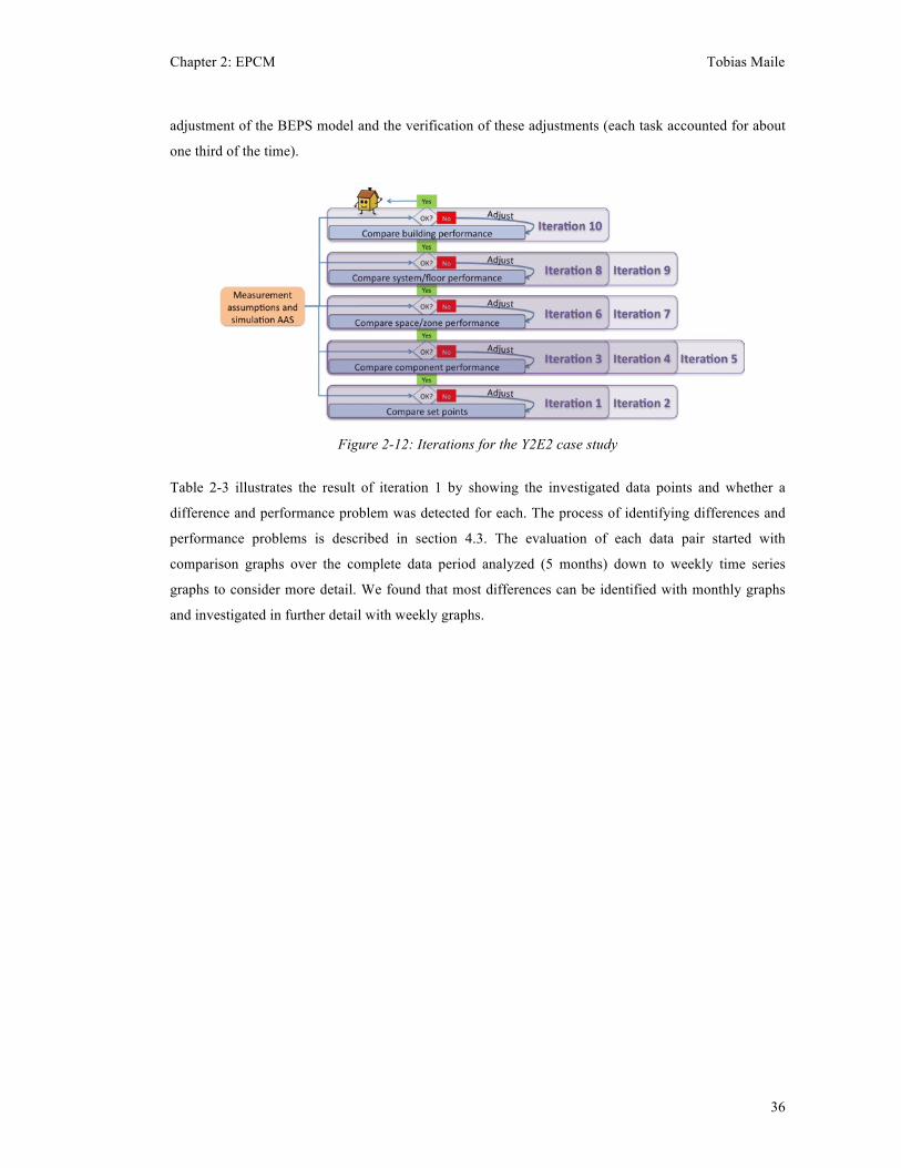
Chapter 2: EPCM Tobias Maile
36
adjustment of the BEPS model and the verification of these adjustments (each task accounted for about
one third of the time).
Figure 2-12: Iterations for the Y2E2 case study
Table 2-3 illustrates the result of iteration 1 by showing the investigated data points and whether a
difference and performance problem was detected for each. The process of identifying differences and
performance problems is described in section 4.3. The evaluation of each data pair started with
comparison graphs over the complete data period analyzed (5 months) down to weekly time series
graphs to consider more detail. We found that most differences can be identified with monthly graphs
and investigated in further detail with weekly graphs.
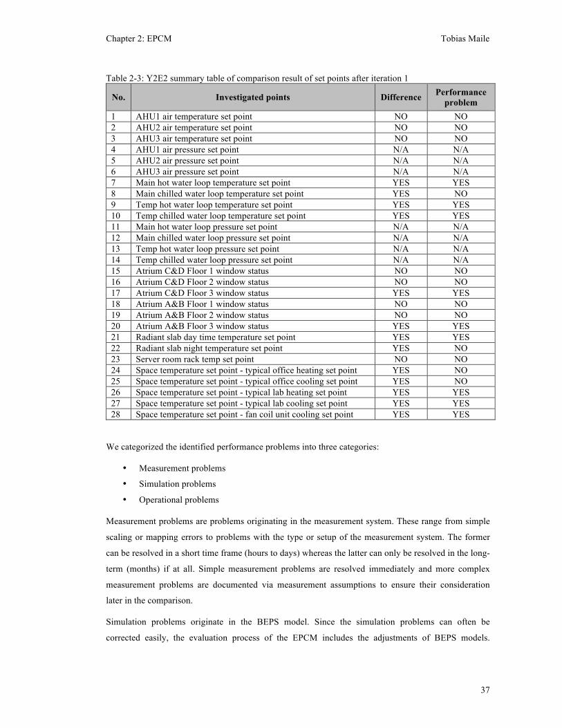
Chapter 2: EPCM Tobias Maile
37
Table 2-3: Y2E2 summary table of comparison result of set points after iteration 1
No. Investigated points Difference Performance problem
1 AHU1 air temperature set point NO NO 2 AHU2 air temperature set point NO NO 3 AHU3 air temperature set point NO NO 4 AHU1 air pressure set point N/A N/A 5 AHU2 air pressure set point N/A N/A 6 AHU3 air pressure set point N/A N/A 7 Main hot water loop temperature set point YES YES 8 Main chilled water loop temperature set point YES NO 9 Temp hot water loop temperature set point YES YES 10 Temp chilled water loop temperature set point YES YES 11 Main hot water loop pressure set point N/A N/A 12 Main chilled water loop pressure set point N/A N/A 13 Temp hot water loop pressure set point N/A N/A 14 Temp chilled water loop pressure set point N/A N/A 15 Atrium C&D Floor 1 window status NO NO 16 Atrium C&D Floor 2 window status NO NO 17 Atrium C&D Floor 3 window status YES YES 18 Atrium A&B Floor 1 window status NO NO 19 Atrium A&B Floor 2 window status NO NO 20 Atrium A&B Floor 3 window status YES YES 21 Radiant slab day time temperature set point YES YES 22 Radiant slab night temperature set point YES NO 23 Server room rack temp set point NO NO 24 Space temperature set point - typical office heating set point YES NO 25 Space temperature set point - typical office cooling set point YES NO 26 Space temperature set point - typical lab heating set point YES YES 27 Space temperature set point - typical lab cooling set point YES YES 28 Space temperature set point - fan coil unit cooling set point YES YES
We categorized the identified performance problems into three categories:
• Measurement problems
• Simulation problems
• Operational problems
Measurement problems are problems originating in the measurement system. These range from simple
scaling or mapping errors to problems with the type or setup of the measurement system. The former
can be resolved in a short time frame (hours to days) whereas the latter can only be resolved in the long-
term (months) if at all. Simple measurement problems are resolved immediately and more complex
measurement problems are documented via measurement assumptions to ensure their consideration
later in the comparison.
Simulation problems originate in the BEPS model. Since the simulation problems can often be
corrected easily, the evaluation process of the EPCM includes the adjustments of BEPS models.
Chapter 2: EPCM Tobias Maile
38
Hereby, input data and tool usage issues can be corrected. Other issues resulting from limitations with
the simulation tool itself are documented via simulations AAS. These BEPS model adjustments aim to
move the BEPS model towards the actual performance and simplify the later comparison process. An
example of a simulation problem was the set point of the hot water loop supply temperature (point no. 7
in Table 2-3 and performance problem no. 19 in Table 2-4). The difference and problem originated in
the control strategy that was implemented in the building and is different from the control strategy of
the design BEPS model.
Operational problems illustrate problems with the actual operation of the building. These are typically
control problems, component problems or problems due to ineffective HVCA system types or
components. An example of an operational problem was the window statuses on the 3rd floor of the
building (point no. 17 in Table 2-3 and performance problem no. 14 in Table 2-4). The actual window
status followed a random pattern and thus showed a difference compared to the simulated window
status.
An example of a difference that is not a problem is an office set point (point no. 24 in Table 2-3). This
difference was caused by the use of different techniques for defining occupied and unoccupied
temperature set points. These different techniques were formulated by the assessor as a simulation
AAS, which explain the difference and indicate that this is not a performance problem.
These discussed performance problems were found during the first iteration of examining the set point
level. By applying the EPCM over all levels of detail, we identified 41 performance problems, which
include the detailed performance problems just discussed (Table 2-4).
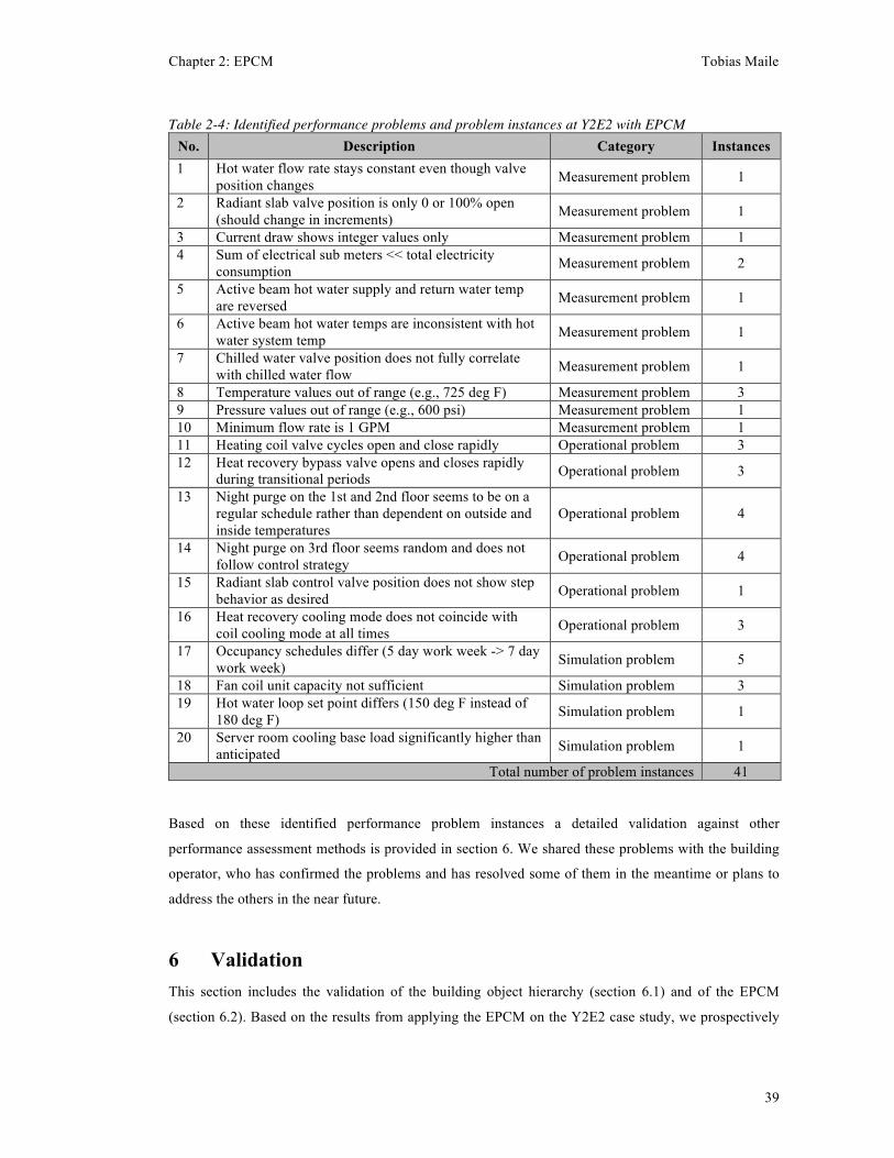
Chapter 2: EPCM Tobias Maile
39
Table 2-4: Identified performance problems and problem instances at Y2E2 with EPCM No. Description Category Instances 1 Hot water flow rate stays constant even though valve
position changes Measurement problem 1
2 Radiant slab valve position is only 0 or 100% open (should change in increments) Measurement problem 1
3 Current draw shows integer values only Measurement problem 1 4 Sum of electrical sub meters << total electricity
consumption Measurement problem 2
5 Active beam hot water supply and return water temp are reversed Measurement problem 1
6 Active beam hot water temps are inconsistent with hot water system temp Measurement problem 1
7 Chilled water valve position does not fully correlate with chilled water flow Measurement problem 1
8 Temperature values out of range (e.g., 725 deg F) Measurement problem 3 9 Pressure values out of range (e.g., 600 psi) Measurement problem 1 10 Minimum flow rate is 1 GPM Measurement problem 1 11 Heating coil valve cycles open and close rapidly Operational problem 3 12 Heat recovery bypass valve opens and closes rapidly
during transitional periods Operational problem 3
13 Night purge on the 1st and 2nd floor seems to be on a regular schedule rather than dependent on outside and inside temperatures
Operational problem 4
14 Night purge on 3rd floor seems random and does not follow control strategy Operational problem 4
15 Radiant slab control valve position does not show step behavior as desired Operational problem 1
16 Heat recovery cooling mode does not coincide with coil cooling mode at all times Operational problem 3
17 Occupancy schedules differ (5 day work week -> 7 day work week) Simulation problem 5
18 Fan coil unit capacity not sufficient Simulation problem 3 19 Hot water loop set point differs (150 deg F instead of
180 deg F) Simulation problem 1
20 Server room cooling base load significantly higher than anticipated Simulation problem 1
Total number of problem instances 41
Based on these identified performance problem instances a detailed validation against other
performance assessment methods is provided in section 6. We shared these problems with the building
operator, who has confirmed the problems and has resolved some of them in the meantime or plans to
address the others in the near future.
6 Validation This section includes the validation of the building object hierarchy (section 6.1) and of the EPCM
(section 6.2). Based on the results from applying the EPCM on the Y2E2 case study, we prospectively
Chapter 2: EPCM Tobias Maile
40
validated the EPCM by comparing it to standard methods used to detect performance problems. On key
characteristic of prospective validation is that results can be presented within a timeframe that allows
practitioners to make business decisions (Ho et al. 2009). This characteristic enabled the improvement
of the building operation of the Y2E2 case study and the verification of actual performance problems
with the building operator. The criteria used for this validation was the number of performance
problems identified and the effort involved to identify this number of performance problems. The result
of the validation indicates that by using the EPCM, the assessor found the largest number of
performance problems, compared to other methods. In particular, the assessor was fastest, on a time
effort per performance problem basis, by applying the EPCM. We also show additional qualitative
evidence that the building object hierarchy supports the understanding of the specific relationships of
building objects on the Y2E2 study. The validation was performed with the help of 11 students, in the
context of a class (CEE243) at Stanford University.
6.1 Validation of the building object hierarchy The building object hierarchy is part of the EPCM, and thus the following validation (section 6.2) of the
EPCM also indirectly validates the building object hierarchy. In addition, the value of the building
object hierarchy was apparent from the feedback of students, who created an instantiation of the
building object hierarchy for the Y2E2 case study in the context of a class. These students used
available documentation, in the form of HVAC system schematics and spreadsheets containing
information about space and zone relationships to HVAC systems, to create an instantiation of the
building object hierarchy. While the source information was accessible to the students before they
created an instantiated hierarchy, they found the process of creating the hierarchy particularly useful for
understanding the different types of relationships among different building objects. While this is only
qualitative evidence, it shows the usefulness of the hierarchy for understanding and documenting
relationships among building objects in a building. Additionally, the building object hierarchy and its
relationships are necessary to identify about 50% of the performance problem instances at Y2E2.
6.2 Validation of the EPCM The prospective validation of a methodology needs to establish that the methodology performs better
for the defined criteria than other methods that address the same problem on the same data set. To
illustrate the value of high level of detail, we also differentiate between problems identified by using the
EPCM over all levels of detail and by using the EPCM at the building and system level only (EPCM
system). We used two criteria to validate the EPCM:
• Number of performance problems
• Time effort per performance problem.
We compared the EPCM to the following methods:

Chapter 2: EPCM Tobias Maile
41
• Building operator (traditional building operation)
• HVAC designer (calibrated BEPS models)
• CEE243 (11 students applying traditional commissioning methods – mainly trend analysis)
• EPCM system level (EPCM with only system level data)
A challenge of such a validation is that it is not known how many performance problems actually exist
within a defined data set. Hereby, we differentiate between problem areas, performance problems and
performance problem instances. Problem areas are broad issues of insufficient performance such as the
building has a heating issue without knowing any details of where this issue originates. A performance
problem is a generic description of a performance inefficiency typically at the component level such as
the natural ventilation control strategy following a different pattern than anticipated. A performance
problem instance is the actual occurrence of a specific performance problem at a specific time at a
specific component (e.g., the control strategy at the 2nd floor atria does not follow the designed control
strategy during the week of April 18th to 25th 2009). To establish a known set of performance problem
instances, we analyzed measured data from Y2E2 with the help of 11 students in the context of a class
(CEE243) based on traditional commissioning methods (mainly trend analysis) and validated the
detected performance problem instances with the building operator. We used this known set of
performance problem instances for comparison with the results obtained by an assessor using EPCM.
Table 2-5 shows the number of performance problem instances identified per problem category. In
comparison to the class results, the HVAC designer identified six possible broader problem areas using
the calibration method, focusing on building and partial system level data. We could verify four out of
the six identified broader problem areas as actual problem instances and found no evidence of actual
problem instances for the other two. The building operator was only aware of two of the identified
performance problem instances. By applying EPCM to the data set, we could identify all of the problem
instances the class identified (except a pressure sensor issue that did not have a corresponding
simulation data point) and even discovered additional problem instances, particularly related to
incorrect design assumptions. These problem instances clearly show the power of the EPCM compared
to a variety of other methods that are currently used in practice. In retrospect, we identified performance
problem instances via EPCM that would not have been found without the use of HVAC component
level data. A comparison between the reduced data set (EPCM system) and the full data set (EPCM)
shows that about half of the problem instances could not be identified without the use of HVAC
component level data. Based on our estimates of time effort, it can be concluded that EPCM is not the
fastest method overall, but it has the best ratio of identified performance problem instance versus time
invested. Future developments and automation of the EPCM will likely decrease the time effort
involved to implement this method.
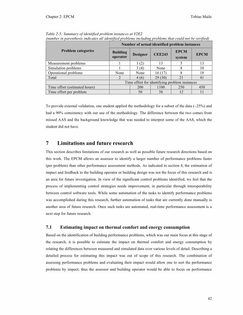
Chapter 2: EPCM Tobias Maile
42
Table 2-5: Summary of identified problem instances at Y2E2 (number in parenthesis indicates all identified problems including problems that could not be verified)
Number of actual identified problem instances Problem categories Building
operator Designer CEE243 EPCM system
EPCM
Measurement problems 1 1 (2) 13 5 13 Simulation problems 1 3 (4) None 8 10 Operational problems None None 16 (17) 8 18 Total 2 4 (6) 29 (30) 21 41 Time effort for identifying problem instances Time effort (estimated hours) 200 1100 250 450 Time effort per problem 50 38 12 11
To provide external validation, one student applied the methodology for a subset of the data (~25%) and
had a 90% consistency with our use of the methodology. The difference between the two comes from
missed AAS and the background knowledge that was needed to interpret some of the AAS, which the
student did not have.
7 Limitations and future research This section describes limitations of our research as well as possible future research directions based on
this work. The EPCM allows an assessor to identify a larger number of performance problems faster
(per problem) than other performance assessment methods. As indicated in section 4, the estimation of
impact and feedback to the building operator or building design was not the focus of this research and is
an area for future investigation. In view of the significant control problems identified, we feel that the
process of implementing control strategies needs improvement, in particular through interoperability
between control software tools. While some automation of the tasks to identify performance problems
was accomplished during this research, further automation of tasks that are currently done manually is
another area of future research. Once such tasks are automated, real-time performance assessment is a
next step for future research.
7.1 Estimating impact on thermal comfort and energy consumption Based on the identification of building performance problems, which was our main focus at this stage of
the research, it is possible to estimate the impact on thermal comfort and energy consumption by
relating the differences between measured and simulated data over various levels of detail. Describing a
detailed process for estimating this impact was out of scope of this research. The combination of
assessing performance problems and evaluating their impact would allow one to sort the performance
problems by impact; thus the assessor and building operator would be able to focus on performance
Chapter 2: EPCM Tobias Maile
43
problems with the highest impact on thermal comfort and energy consumption. We see this as a fruitful
area for future research.
7.2 Feedback based on identified performance problems While we have not looked at a detailed process for how best to provide feedback on the building design
and the building operation, the identified performance problems provide a basis for such a feedback. In
our case studies, we have used an informal approach to communicate performance problems that we
found with building operators and building designers. This communication indicates a first step towards
closing the gap between building design and operation. One example of such an important lesson is our
evaluation of the energy consumption of a server room that used about 50% of the base-cooling load of
the building. Despite its importance for energy consumption, the server room was not included in the
design BEPS model, which made it practically impossible to predict building energy consumption
accurately during design, since a major source of energy consumption was not included in the BEPS
model. Although feedback to building design was out of scope of this research, future researchers could
look into ways to efficiently provide feedback to building designers and explore ways that they can
learn from this feedback.
7.3 Better integration with controls The disconnect between actual controls and the controls available in the BEPS tool was apparent from
the case studies. Interoperability between design HVAC control tools, control of BEPS, and actual
control algorithms with the control hardware of a building could eliminate errors in the current process
of implementing control strategies. Finding new ways to share control strategies across tool boundaries
would improve the reliability of control strategies in buildings and decrease errors that occur with the
current manual implementation of controls.
7.4 Automation of EPCM One major topic for future research is the automation of the EPCM. Figure 2-3 indicates the tasks we
automated. We spent considerable time developing data transformation software tools that ease the
generation of the input to BEPS tools, support data transformation such as unit conversions, update
simulation input data, and graph data. The integration of all these tools into a comprehensive user
interface that supports all aspects of the EPCM is another area for possible future research. Due to the
time effort of performing manual tasks such as detecting differences of data pairs, we did not analyze
all available data for the building (only about 30% of the available data points over a 5 months period).
With more automation, the complete analysis of all data would become more manageable.
Chapter 2: EPCM Tobias Maile
44
7.5 Real-time energy performance assessment Once the EPCM is completely automated, a real-time performance assessment based on design BEPS
models becomes possible and may provide crucial timely information to the building operator. With
estimation of the impact of performance problems in addition to automation of the EPCM, it will be
possible to determine the severity of performance problems. Based on this information, the automated
EPCM could provide the building operator with timely information about the most important
performance problems. A fully automated EPCM could also determine whether control changes in the
building have the effects that were expected based on simulated performance.
8 Conclusion To compare measured and simulated data the EPCM includes steps and tasks that systematically
eliminate or highlight inappropriate simulation approximations, assumptions, and simplifications in a
BEPS model and highlight inappropriate measurement assumptions, so that it is worthwhile to examine
the remaining differences more closely to identify actual performance problems. By aligning the BEPS
model as closely as possible to the actual situation in the building, it becomes a much more useful tool
for finding performance problems. This paper describes the key novel concepts and processes that
enable this systematic adjustment of the BEPS model so that it matches actual building conditions as
closely as possible. The two contributions of this paper are the Energy Performance Comparison
Methodology (EPCM) and the building object hierarchy that integrates two perspectives (HVAC and
spatial). The EPCM allows an assessor to identify a larger number of performance problems with a
lower time effort per performance problem compared to other standard methods, by comparing
measured and simulated building energy performance data. It includes details about the process for
assessing performance data, including a bottom-up approach for iteratively adjusting the BEPS model.
The key aspect of this methodology is that through iterative adjustments, the BEPS model moves from a
design BEPS model to a BEPS model that more closely simulates actual building performance.
Existing building object hierarchies mostly concern only one perspective. O'Donnell (2009) combines
two perspectives (HVAC and spatial), focused on the zone object. We developed a building object
hierarchy that provides two perspectives (spatial and thermal) that are linked on the zone and space
levels and provide additional relationships among objects that are not contained in other hierarchies. For
the validation case study, the building object hierarchy provided relationships that are needed to find
about 50% of the performance problem instances.
Existing approaches to compare simulated with measured data fall short of including details over all
levels of detail and often do not consider design BEPS models. We have developed a methodology that
includes those details and a link to design BEPS models, and enables the systematic identification of
performance problems. The EPCM, combined with the knowledge of measurement assumptions and

Chapter 2: EPCM Tobias Maile
45
simulation AAS, enables a better understanding of the differences between measured and simulated
data and allows the assessment of building energy performance compared to design. The EPCM still
contains manual tasks, but future developments could increase the automation of tasks and decrease the
time effort involved. With additional automation, future investigations will lead to real-time
performance assessment. More importantly, the EPCM is a step in closing the gap between design
simulation and actual operation, which is becoming more important as new regulations and
requirements are developed to save energy in buildings.
9 Bibliography Austin, S.B. (1997). HVAC system trend analysis. ASHRAE Journal, 39(2), 44-50.
Bazjanac, V., and T. Maile. (2004). IFC HVAC interface to EnergyPlus -A case of expanded
interoperability for energy simulation. Proceedings of the Simbuild 2004, 31-37. Boulder, CO:
International Building Performance Simulation Association (IBPSA).
Bensouda, N. (2004). Extending and formalizing the energy signature method for calibrating
simulations and illustrating with application for three California climates. Master Thesis,
College Station, TX: Texas A&M University.
Cho, S.Y. (2002). The persistence of savings obtained from commissioning of existing buildings.
Master thesis, Bryan, TX: Texas A&M University.
Clarke, J.A. (2001). Energy simulation in building design. Oxford, UK: Butterworth-Heinemann.
Crawley, D.B., J.W. Hand, and L.K. Lawrie. (1999). Improving the weather information available to
simulation programs. Proceedings of Building Simulation 1999, 2, 529–536. Kyoto, Japan:
International Building Performance Simulation Association (IBPSA).
Duffie, J.A., and W.A. Beckman. (1980). Solar engineering of thermal processes. New York, NY: John
Wiley & Sons.
Frank, M., H. Friedman, K. Heinemeier, C. Toole, D. Claridge, N. Castro, and P. Haves. (2007). State-
of-the-art review for commissioning low energy buildings: Existing cost/benefit and
persistence methodologies and data, state of development of automated tools and assessment
of needs for commissioning ZEB. NISTIR #7356. Gaithersburg, MD: National Institute of
Standards and Technology (NIST).
Grob, R.F., and M. Madjidi. (1997). Commissioning and fault detection of HVAC systems by using
simulation models based on characteristic curves. Proceedings of the Clima 2000 Conference.
Brussels.

Chapter 2: EPCM Tobias Maile
46
Ho, P., Fischer, M., and Kam, C. (2009). “Prospective validation of VDC methods: Framework,
application, and implementation guidelines.” Working Paper #123. Stanford, CA: Center for
Integrated Facility Engineering, Stanford University.
Husaunndee, A., R. Lahrech, H. Vaezi-Nejad, and J.C. Visier. (1997). SIMBAD: A simulation toolbox
for the design and test of HVAC control systems. Proceedings of the 5th international IBPSA
conference, 2, 269–276. Prague, Czech Republic: International Building Performance
Simulation Association (IBPSA).
Hyvarinen, J., and S. Karki. (1996). Building optimization and fault diagnosis source book. IEA Annex
#25. Espoo, Finland: International Energy Agency (IEA).
IDS. (2004). Defining the next generation enterprise energy management system. White paper.
Waltham, MA: Interval Data Systems, August.
Katipamula, S., M.R. Brambley, N.N. Bauman, and R.G. Pratt. (2003). Enhancing building operations
through automated diagnostics: Field test results. Proceedings of the 3rd International
Conference for Enhanced Building Operations, 114-126. Berkeley, CA: Energy Systems
Laboratory.
Kunz, J., T. Maile, and V. Bazjanac. (2009). Summary of the energy analysis of the first year of the
Stanford Jerry Yang & Akiko Yamazaki Environment & Energy (Y2E2) Building. Technical
Report #183. Stanford, CA: Center for Integrated Facility Engineering, Stanford University.
http://cife.stanford.edu/online.publications/TR183.pdf last accessed on March 15, 2010.
Maile, T., V. Bazjanac, M. Fischer, and J. Haymaker. (2010a). Formalizing approximation,
assumptions, and simplifications to document limitations in building energy performance
simulation. Working Paper #126. Stanford, CA: Center for Integrated Facility Engineering,
Stanford University.
Maile, T., M. Fischer, and V. Bazjanac. (2010b). Formalizing assumptions to document limitations of
building performance measurement systems. Working Paper #125. Stanford, CA: Center for
Integrated Facility Engineering, Stanford University.
Marion, W., and K. Urban. (1995). Users manual for TMY2s: Derived from the 1961–1990 National
Solar Radiation Data Base. Technical Report #463. Golden, CO: National Renewable Energy
Laboratory.

Chapter 2: EPCM Tobias Maile
47
Mills, E., N. Bourassa, M.A. Piette, H. Friedman, T. Haasl, T. Powell, and D. Claridge. (2005). The
cost-effectiveness of commissioning new and existing commercial buildings: Lessons from
224 buildings. Proceedings of the 2005 National Conference on Building Commissioning, 495-
516. New York, NY: Portland Energy Conservation Inc.
http://www.peci.org/ncbc/proceedings/2005/19_Piette_NCBC2005.pdf last accessed on March
15, 2010.
O'Donnell, J. (2009). Specification of optimum holistic building environmental and energy performance
information to support informed decision making. Ph.D. Thesis, Department of Civil and
Environmental Engineering, University College Cork (UCC), Ireland.
Persson, B. (2005). Sustainable City of Tomorrow - B0-01 - Experiences of a Swedish housing
exposition. Stockholm, Sweden: Swedish Research Council, Distributed by Coronet Books.
Piette, M.A., S. Kinney, and P. Haves. (2001). Analysis of an information monitoring and diagnostic
system to improve building operations. Energy and Buildings, 33(8), 783-791.
Reddy, T. (2006). Literature review on calibration of building energy simulation programs: uses,
problems, procedures, uncertainty and tools. ASHRAE Transactions, 112(1), 226-240.
Salsbury, T., and R. Diamond. (2000). Performance validation and energy analysis of HVAC systems
using simulation. Energy & Buildings, 32(1), 5–17.
Santos, J.J., and J. Rutt. (2001). Preparing for Diagnostics from DDC Data–PACRAT. Proceedings of
the 9th National Conference on Building Commissioning, 9–11. Cherry Hill, NJ: Portland
Energy Conservation Inc (PECI).
Scofield, J.H. (2002). Early performance of a green academic building. ASHRAE Transactions, 108(2),
1214–1232.
Seidl, R. (2006). Trend analysis for commissioning. ASHRAE Journal, 48(1), 34-43.
U.S. DOE. (2010). EnergyPlus - Engineering Reference.
http://apps1.eere.energy.gov/buildings/energyplus/pdfs/engineeringreference.pdf last accessed
on May 21, 2010.
Visier, J., J. Lebrun, P. André, D. Choiniere, T. Salsbury, H. Vaézi-Néjad, P. Haves, et al. (2004).
Commissioning tools for improved energy performance. Technical Report. IEA ECBCS Annex
#40. Marne la Vallée Cedex, France: International Energy Agency (IEA) - Energy
Conservation in Buildings & Community Systems (ECBCS).
http://www.ecbcs.org/docs/Annex_40_Commissioning_Tools_for_Improved_Energy_Perform
ance.pdf last accessed on May 14, 2009.

Chapter 2: EPCM Tobias Maile
48
Wang, F., H. Yoishida, S. Masuhara, H. Kitagawa, and K. Goto. (2005). Simulation-based automated
commissioning method for air-conditioning systems and its application case study.
Proceedings of the 9th IBPSA conference, 1307-1314. Montreal, Canada: International
Building Performance Simulation Association.
Xu, P., P. Haves, and M. Kim. (2005). Model-based automated functional testing-methodology and
application to air handling units. ASHRAE Transactions, 111(1), 979-989.
Yin, R.K. (2003). Case study research: Design and methods. 3rd ed. Thousand Oaks, CA: Sage
Publications.
Chapter 3: Measurement assumptions Tobias Maile
49
Chapter 3: Formalizing assumptions to document limitations
of building performance measurement systems
Tobias Maile, Martin Fischer, Vladimir Bazjanac
1 Abstract Building energy performance is often unknown or inadequately measured. When performance is
measured, it is critical to understand the validity of the measured data before identifying performance
problems. Limitations of measurement systems make adequate assessment of validity difficult. These
limitations originate in the set of available data and in the functional parts of the measurement system.
Previous research has used project-specific assumptions in an ad-hoc manner to describe these
limitations, but the research has not compiled a list of critical measurement assumptions and a process
to link the measurement assumptions to performance problems. To aid in the assessment of measured
data, we present a list of critical measurement assumptions drawn from the existing literature and four
case studies. These measurement assumptions describe the validity of measured data. Specifically, we
explain the influence of sensing, data transmission, and data archiving. We develop a process to identify
performance problems resulting from differences between measured and simulated data using the
identified measurement assumptions. This paper validates existing measurement data sets based on
known performance problems in a case study and shows that the developed list of critical measurement
assumptions enables the identification of differences caused by measurement assumptions and exclude
them from analysis of potential performance problems.
2 Introduction Assessing building energy performance requires adequate measured data from a building. Previous
studies report problems with measurement data or missing measurements in commercial buildings. For
example, Torcellini et al. (2006) describe several problems with measurement systems for six case
studies. O'Donnell (2009) document measurement problems as well, but also discuss consequences of
missing measurement data. These reported measurement problems are the result of limitations of
measurement systems that can be described with measurement assumptions. Previous research in this
area has not used a common set of measurement assumptions. In fact, assumptions have been
mentioned rarely, and then only in a project-specific contexts (e.g., Salsbury and Diamond 2000).
Measurement assumptions must be articulated to link the measurement system to the real world (the
actual building). When clearly articulated, assumptions can explain limitations of measurement systems
Chapter 3: Measurement assumptions Tobias Maile
50
and resulting measurement data. This helps building energy professionals to understand differences
between measured and simulated building energy performance data. While this paper focuses on
measurement assumptions, Maile et al. (2010a) detail simulation approximations, assumptions, and
simplifications, and Maile et al. (2010b) discuss a comparison methodology based on measured and
simulated data. A person that we call a performance assessor, who could be either a commissioning
expert and/or a control system expert, would perform or supervise the tasks involved to document
measurement assumptions for the comparison of measured and simulated data.
A measurement system consists of a measurement data set in the form of sensor data and control data
(e.g., set points), transmission of the data, and data storage where data are archived for later use. All
parts of a measurement system have a specific function that may or may not be fulfilled continuously
over time. The resulting quality of the archived data depends on the use of a measurement system that
works with sufficient reliability overall and in each part. Limitations or shortcomings of measurement
systems have often been described as measurement errors. Reddy et al. (1999) categorized measurement
errors as errors of calibration, data acquisition, and data reduction but did not mention errors in the
sensor product itself. While sensor errors can be described quantitatively, assumptions provide only
qualitative descriptions of a given limitation.
The basis for each measurement system is the measurement data set, which is defined by the number of
sensors, sensor types, sensor placement, and sensor accuracy. Several guidelines exist that define
measurement data sets (Barley et al. 2005; Gillespie et al. 2007; Neumann and Jacob 2008; O'Donnell
2009). While all of these guidelines address the questions of which physical variables should be
measured by which sensor types and how often, only some contain detailed information about sensor
placement and recommended sensor accuracy. In addition, only some guidelines consider control points
such as set points as part of the data set. Previous validation of these guidelines has not been
comprehensive, in that the guidelines were not compared to other guidelines or to actual building case
studies. Measurement assumptions must be closely tied to measurement data sets and guidelines, since
the characteristics of sensors (such as placement, accuracy, or product type) define the basic limitations
of measurement systems. The ability to detect performance problems depends greatly on the available
data set, since inconsistencies can only be detected when the related parameters are actually measured.
Transmission of the sensor output data usually occurs within the control system and/or the data
acquisition system. Some possible major limitations related to transmission are related to the bandwidth
(Gillespie et al. 2007), hardware, and software of the control or data acquisition system. These
limitations may reduce data quality or lead to data loss.
Data storage also plays a significant role in the quality of resulting measurement data and thus is
another source of potential limitations to the measurement system. Different measurement systems
archive data in different formats (Friedman and Piette 2001), but all contain at least a set of data
Chapter 3: Measurement assumptions Tobias Maile
51
comprising a timestamp and a sensed value. The time interval and format of the timestamp define the
temporal granularity of the recorded data. The archival type of the value may or may not be consistent
with the resolution of the sensed and transmitted data values. These inconsistencies lead to inaccurate
measurements, inconsistent temporal resolution and loss of data.
Due to the described limitations of measurement systems, the reliability of archived data varies across
buildings and over time. Reliability of a measurement system describes the consistency of archived data
both in the number of archived data points per time interval and in the variability of this number over
time. For example, Olken et al. (1998) reported reliability issues with measurement systems. The
reliability of measurement systems is an important characteristic, since more data loss leads to less
information about the performance of a building.
In this paper, we discuss, summarize, and then validate the existing guidelines for measurement data
sets (see section 3.1). In addition, we mention the extent to which these guidelines include information
about the possible limitations of the measurement system. We illustrate how to use these guidelines to
develop a measurement data set for a project (see section 3.2) to minimize limitations. We discuss in
detail the limitations of the three main functions of a measurement system: sensing (section 3.3),
transmitting (section 3.4), and archiving (section 3.5). We describe the process to use measurement
assumptions to assess difference between measured and simulated data (section 3.6). Given all of the
described sources of limitations of measurement systems, we will develop a list of critical measurement
assumptions based on the existing literature and on four building case studies (section 3.7). We
categorize this list of assumptions according to the three main functions of a measurement system. In
view of the variety of problems and limitations with measurement systems, we illustrate how to verify a
measurement system based on existing methods (section 3.8) and define a reliability measure that
quantitatively describes the reliability of the archived data (section 3.9).
We based our research on case studies to provide real-life context (Yin 2003) for observing problems
and limitations with measurement systems. The research method typically used in this research area is a
single case study. Survey- or interview-based methods are not applicable, due to the limited existing
knowledge about and lack of standard practice regarding measurement assumptions. Thus, we observed
current practice with four case studies. In section 4, we provide a description of each building, the
measurement data set, and the data acquisition system for each case study. We highlight the specific
limitations of each measurement system and the correlated measurement assumptions.
Based on the first two case studies, we developed a concept for the measurement assumptions and
observed measurement systems. One later case study was used to prospectively validate this concept.
The fourth case study is in progress, but is already presented in this paper since it adds to the generality.
In section 5.1, we present a validation of the existing guidelines for measurement data sets based on
known performance problems as well as a validation of measurement assumptions based on the number
Chapter 3: Measurement assumptions Tobias Maile
52
of times when measurement assumptions can explain differences between measured and simulated data
in a case study (section 5.2). The use of multiple case studies of different building types (office, mixed-
use research and office, correctional) and different heating, ventilation, and air conditioning (HVAC)
systems (natural ventilation, mixed natural and mechanical ventilation, and only mechanical ventilation)
provides more generality for our results compared to an approach involving a single case study. After
describing details of the validation, we discuss recommendations (section 6) and provide limitations and
suggestions for possible future research (section 7).
3 Measurement systems and their limitations This section details the different sources of measurement assumptions that are based in limitations of
the measurement system. Since limitations depend on the types and numbers of sensors within a
measurement system, we first discuss existing guidelines (section 3.1) that define measurement data
sets and describe how to establish such a data set for a given case study (section 3.2). These data sets
consist of mechanical sensors, which are defined as devices that respond to a physical stimulus and
transmits a resulting impulse (Sensor 2010). These mechanical sensors enable an automated, continuous
and effortless (excluding installation and maintenance) collection of the resulting data. Human
observations may extend these data sets with useful information, but due to the related effort and
subjectivity are out of focus of this paper. We discuss details of sensor accuracy (section 3.3), data
transmission (section 3.4), and archiving (section 3.5). We discuss the process to identify performance
problems (section 3.6) and provide a list of critical measurement assumptions (section 3.7). This paper
also describes existing methods to verify the functionality of measurement systems (section 3.8) and
defines a reliability measure for them (section 3.9).
3.1 Existing measurement data sets Due to inconsistencies and differences in measurement data sets used across buildings in current
practice (Brambley et al. 2005), several authors have proposed guidelines and procedures defining
measurement data sets for different purposes in recent years. The standard practice of measurement in
buildings is to collect data for billing (utility data set) and for ad-hoc measurements (HVAC control
system data set). We describe these standard data sets as well as existing measurement guidelines
reported in the literature. Through the description of these data sets we show that buildings already
contain measurement data (while the data may not be archived) and that several different guidelines
exists that guide building owners for selection of additional measurement data that are useful for their
buildings. The resulting list of measurement data sets is:
• Utility data set
• HVAC control system (Underwood 1999) data set

Chapter 3: Measurement assumptions Tobias Maile
53
• Guidelines for the evaluation of building performance (Neumann and Jacob 2008) data set
• Procedure for measuring and reporting commercial building energy performance (Brambley et
al. 2005) data set
• Guide for specifying performance monitoring systems in commercial and institutional
buildings (Gillespie et al. 2007) data set
• Ideal data set (O'Donnell 2009)
These different data sets exist for different purposes. The utility data set is used to determine the total
energy consumption of a building to establish a basis for billing. The HVAC control system data set is
needed for the operation and control of an HVAC system. The listed guidelines from the literature aim
to establish data sets that support either the evaluation of building energy performance and/or the
identification of performance problems. The analysis process of these guidelines ranges from
benchmarking to the use of calibrated simulation models. While benchmarking is the comparison of
actual building performance to comparable benchmarks such as corresponding standards or comparable
buildings, calibrated simulation models try to match actual performance with simulated performance.
Maile et al. (2010b) provide a more detailed discussion of existing comparison methods.
Typically, a measurement data set is characterized by:
• number of sensors
• types of sensors
• sensor placement
• sensor characteristics (accuracy and resolution)
• time interval
• installation costs
• maintenance cost
A good guideline for a measurement data set should provide information on all of the above
characteristics. At a minimum, the existing guidelines for measurement data sets must describe the
types of measurements, number of measurements, and recommended time intervals. However, the
guidelines are inconsistent in providing further details. Some include information about installation
costs, sensor placement, and sensor characteristics (accuracy and resolution). Table 3-1 summarizes
the available characteristics for a measurement data set for each of the guidelines.
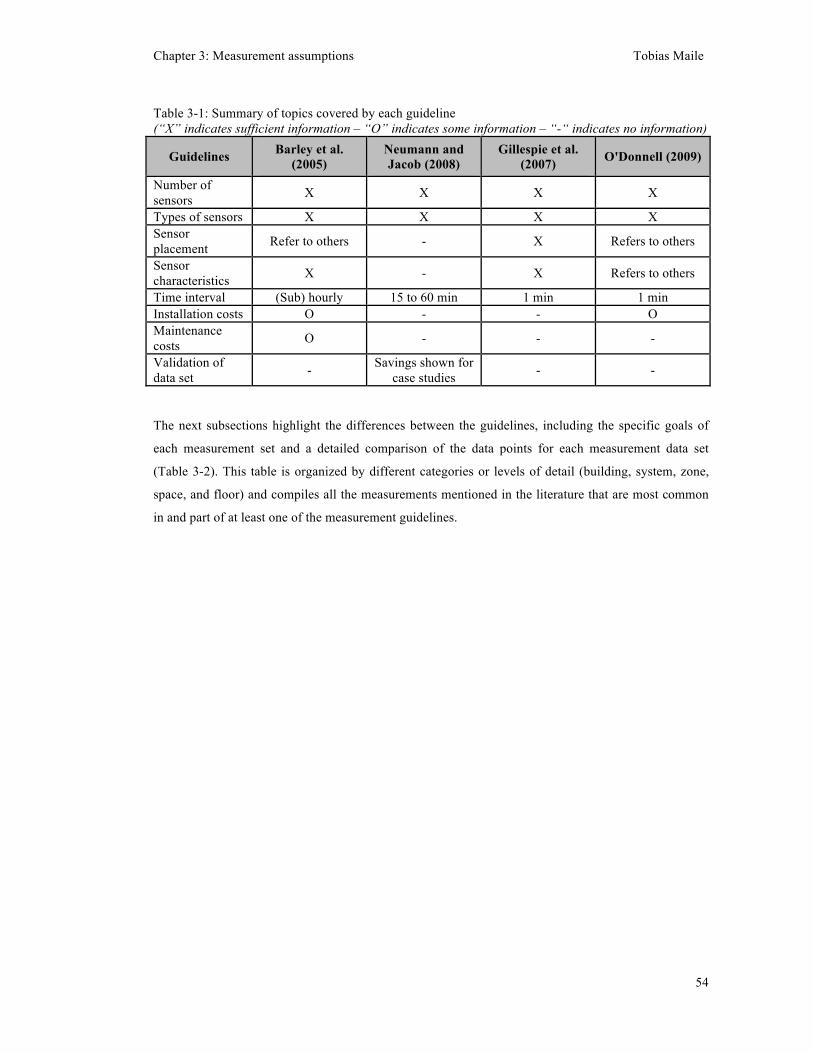
Chapter 3: Measurement assumptions Tobias Maile
54
Table 3-1: Summary of topics covered by each guideline (“X” indicates sufficient information – “O” indicates some information – “-“ indicates no information)
Guidelines Barley et al. (2005)
Neumann and Jacob (2008)
Gillespie et al. (2007) O'Donnell (2009)
Number of sensors X X X X
Types of sensors X X X X Sensor placement Refer to others - X Refers to others
Sensor characteristics X - X Refers to others
Time interval (Sub) hourly 15 to 60 min 1 min 1 min Installation costs O - - O Maintenance costs O - - -
Validation of data set - Savings shown for
case studies - -
The next subsections highlight the differences between the guidelines, including the specific goals of
each measurement set and a detailed comparison of the data points for each measurement data set
(Table 3-2). This table is organized by different categories or levels of detail (building, system, zone,
space, and floor) and compiles all the measurements mentioned in the literature that are most common
in and part of at least one of the measurement guidelines.
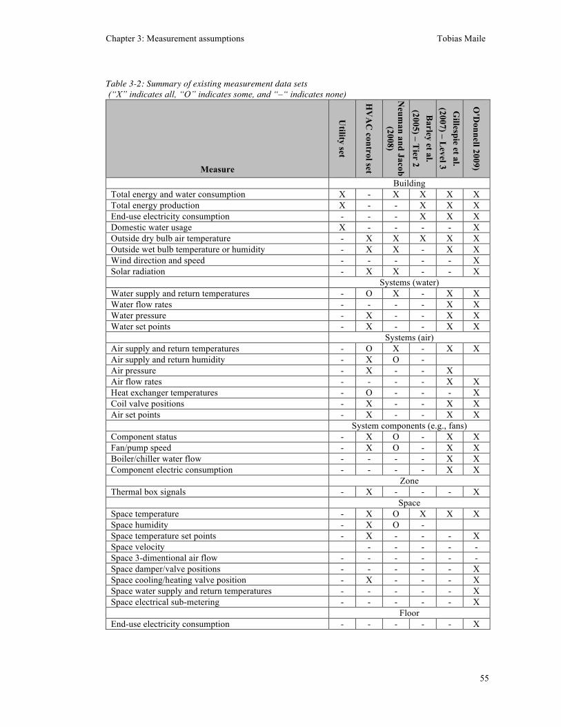
Chapter 3: Measurement assumptions Tobias Maile
55
Table 3-2: Summary of existing measurement data sets (“X” indicates all, “O” indicates some, and “–“ indicates none)
Measure
Utility set
HV
AC
control set
Neum
an and Jacob (2008)
Barley et al.
(2005) – Tier 2
Gillespie et al.
(2007) – Level 3
O'D
onnell 2009)
Building Total energy and water consumption X - X X X X Total energy production X - - X X X End-use electricity consumption - - - X X X Domestic water usage X - - - - X Outside dry bulb air temperature - X X X X X Outside wet bulb temperature or humidity - X X - X X Wind direction and speed - - - - - X Solar radiation - X X - - X Systems (water) Water supply and return temperatures - O X - X X Water flow rates - - - - X X Water pressure - X - - X X Water set points - X - - X X Systems (air) Air supply and return temperatures - O X - X X Air supply and return humidity - X O - Air pressure - X - - X Air flow rates - - - - X X Heat exchanger temperatures - O - - - X Coil valve positions - X - - X X Air set points - X - - X X System components (e.g., fans) Component status - X O - X X Fan/pump speed - X O - X X Boiler/chiller water flow - - - - X X Component electric consumption - - - - X X Zone Thermal box signals - X - - - X Space Space temperature - X O X X X Space humidity - X O - Space temperature set points - X - - - X Space velocity - - - - - Space 3-dimentional air flow - - - - - - Space damper/valve positions - - - - - X Space cooling/heating valve position - X - - - X Space water supply and return temperatures - - - - - X Space electrical sub-metering - - - - - X Floor End-use electricity consumption - - - - - X
Chapter 3: Measurement assumptions Tobias Maile
56
3.1.1 Utility data set
The utility data set is needed to establish a basis for billing. It includes measurements for total building
electricity and any other energy sources (such as, for example, chilled water, natural gas, or oil) that the
building uses and are typically recorded at a monthly and/or annual interval. Depending on the
breakdown of billing entities in a building, this data set may also include additional sub-meters. A
validation of the utility data set is of little use, since it mainly includes total building-level
measurements and additional sub-metering based on the breakdown of building objects. Placement of
these sensors is typically at the building level and occasionally on a floor level, depending on the tenant
distribution. Every building has a utility data set at the building level (sometimes multiple buildings are
combined) that is archived typically on a monthly or annual basis for billing purposes.
3.1.2 HVAC control data set
The HVAC control measurement data set provides the feedback necessary for the control of the
building (Underwood 1999). An example measurement point in this data set is an air temperature sensor
in a space. Depending on that temperature measurement, the control system activates a set of
components that allow for a change in the supply of heating or cooling air for that space. Typically, a
corresponding set point defines the temperature or temperature range as the goal for the system to
achieve. The point list of a building contains the measurements and control points of the control system.
These necessary measurements for controlling an HVAC system typically include space air
temperature, air loop supply temperature, system water temperature (supply and sometimes return), and
absolute or differential system pressure. In addition to the mentioned set points, HVAC systems
typically include a range of other control points that actuate specific components, such as valves,
dampers, or fans. These control points describe the theoretical or goal state of the system, whereas
sensors determine the actual state of a component, variable, or system. The HVAC control data set of
measurements and control signals is the basis of operation for every HVAC system, and it is a
fundamental part of a measurement data set. Typically, these data points are available in the control
system, but the resulting data are not archived. Placement and accuracy goals may be included in design
documentation or project specifications. The HVAC control data set is usually not validated in practice
on completeness, accuracy and placement, since this has not been a major focus in buildings.
3.1.3 Guidelines for the Evaluation of Building Performance
According to Neumann and Jacob (2008), the goal of these guidelines is to enable a “rough overall
assessment of the performance of the system.” Neumann and Jacob use a top-down approach from
benchmark comparisons to calibrated models, leading into ongoing. Their assessment is based on a so-
called minimum data set that contains only a few measurements to keep measurement system costs to a
minimum. Those are mainly building level measurements, such as primary energy consumption and
Chapter 3: Measurement assumptions Tobias Maile
57
some system- and space-level temperature measurements. The suggested time interval is between 15
minutes and an hour. A validation of the usefulness of these guidelines is indicated by early results that
show 10-20% total energy savings in demonstration buildings (Schmidt et al. 2009). However, the
authors did not validate their guidelines against other approaches. These guidelines do not contain any
information about placement or accuracy of sensors.
3.1.4 Procedure for Measuring and Reporting Commercial Building Energy Performance
Barley et al. (2005) state that this procedure provides a “method for measuring and characterizing the
energy performance of commercial buildings” and, therefore, defines a set of performance metrics. It
also includes the necessary details on measurements for each performance metric. It defines two
different tiers of measurement. Tier 1 focuses on building-level energy consumption. Tier 2 includes
additional temporary sub-meters for energy consumption. Besides a difference in sensor and installation
costs, the authors did not mention any other reasons to choose one tier over the other. The authors did
not provide any validation of their measurement data sets other than describing an example building, its
performance metrics, and the fact that the performance metrics seem to follow their expectations. The
requested time interval for the data ranges from monthly (Tier 1) to (sub-)hourly (Tier 2). These
guidelines contain a detailed discussion about sensor accuracy and some specific recommendations for
selected sensor products. For sensor placement, Barley et al. mainly refer to manufacturer
specifications.
3.1.5 Guide for Specifying Performance Monitoring Systems in Commercial and
Institutional Buildings
The Guide for Specifying Performance Monitoring Systems in Commercial and Institutional Buildings
(Gillespie et al. 2007) focuses on the requirements for a monitoring system that supports ongoing
commissioning. It includes additional measurements compared to the procedures described above, such
as measures of air and water flows as well as measures of power consumption of specific HVAC
equipment, taken on a system level as a basic level of monitoring. The authors define three monitoring
levels, essential, progressive, and sophisticated, to allow for different monitoring project scenarios.
They do not provide any validation of these guidelines. Gillespie et al. (2007) recommend a one-minute
interval. These guidelines contain specific information about sensor accuracy and placement but not
about the costs of measurement systems.
3.1.6 Ideal data set and actor view
O’Donnell (2009) defines a so-called ideal measurement data set that includes a maximum set of
measurements. While it is apparent that such an ideal set of measurements is very intensive in terms of
the number of sensor products, installation costs, and control system capability, it provides a good
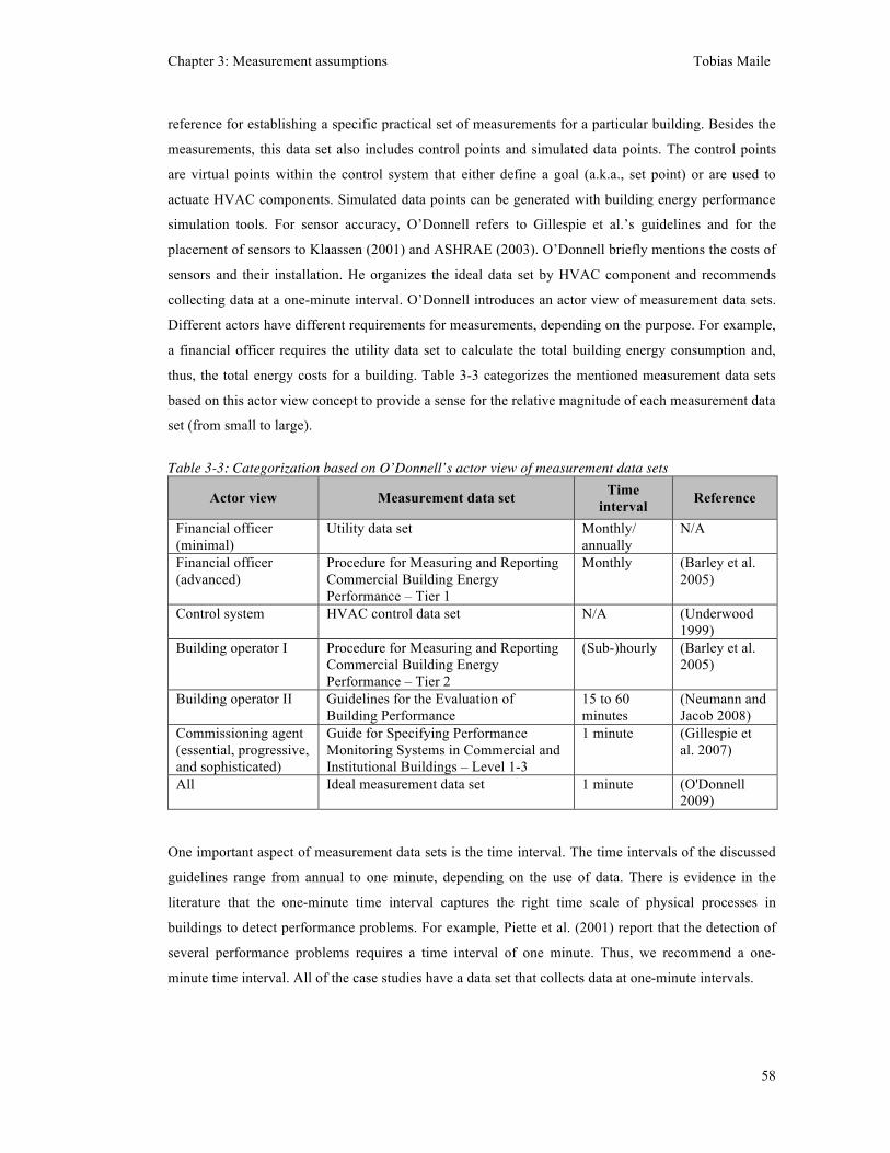
Chapter 3: Measurement assumptions Tobias Maile
58
reference for establishing a specific practical set of measurements for a particular building. Besides the
measurements, this data set also includes control points and simulated data points. The control points
are virtual points within the control system that either define a goal (a.k.a., set point) or are used to
actuate HVAC components. Simulated data points can be generated with building energy performance
simulation tools. For sensor accuracy, O’Donnell refers to Gillespie et al.’s guidelines and for the
placement of sensors to Klaassen (2001) and ASHRAE (2003). O’Donnell briefly mentions the costs of
sensors and their installation. He organizes the ideal data set by HVAC component and recommends
collecting data at a one-minute interval. O’Donnell introduces an actor view of measurement data sets.
Different actors have different requirements for measurements, depending on the purpose. For example,
a financial officer requires the utility data set to calculate the total building energy consumption and,
thus, the total energy costs for a building. Table 3-3 categorizes the mentioned measurement data sets
based on this actor view concept to provide a sense for the relative magnitude of each measurement data
set (from small to large).
Table 3-3: Categorization based on O’Donnell’s actor view of measurement data sets
Actor view Measurement data set Time interval Reference
Financial officer (minimal)
Utility data set Monthly/ annually
N/A
Financial officer (advanced)
Procedure for Measuring and Reporting Commercial Building Energy Performance – Tier 1
Monthly (Barley et al. 2005)
Control system HVAC control data set N/A (Underwood 1999)
Building operator I Procedure for Measuring and Reporting Commercial Building Energy Performance – Tier 2
(Sub-)hourly (Barley et al. 2005)
Building operator II Guidelines for the Evaluation of Building Performance
15 to 60 minutes
(Neumann and Jacob 2008)
Commissioning agent (essential, progressive, and sophisticated)
Guide for Specifying Performance Monitoring Systems in Commercial and Institutional Buildings – Level 1-3
1 minute (Gillespie et al. 2007)
All Ideal measurement data set 1 minute (O'Donnell 2009)
One important aspect of measurement data sets is the time interval. The time intervals of the discussed
guidelines range from annual to one minute, depending on the use of data. There is evidence in the
literature that the one-minute time interval captures the right time scale of physical processes in
buildings to detect performance problems. For example, Piette et al. (2001) report that the detection of
several performance problems requires a time interval of one minute. Thus, we recommend a one-
minute time interval. All of the case studies have a data set that collects data at one-minute intervals.

Chapter 3: Measurement assumptions Tobias Maile
59
3.1.7 Summary of measurement data sets
Figure 3-1 presents a graphical overview of all data sets discussed that illustrates their relationships and
the extent to which they include control signals, measured data, and simulated data. While all guidelines
contain data points from measurements, only O’Donnell’s ideal data set defines the data points for
simulated data. Barley et al. use set points only as a reference if corresponding measurements are not
available. Gillespie et al. and Neumann and Jacob include some space level information, while Barley
et al. do not. Gillespie et al. and O’Donnell include set points in their measurement data sets. Set points
are important, since they define the goal that the HVAC system aims to achieve. The need for simulated
data points is inherent in the concept of comparison measured with simulated data. Section 5.1
compares these guidelines to the measurement data sets of the four case studies. In addition, we provide
validation based on the identified performance problems of a case study.
Figure 3-1: Overview of different measurement data sets
3.2 Selecting data points for performance evaluation We used the following process to select the measurements for the case studies. If a point list for the
building and mechanical drawings existed, the first task was to extract HVAC components from
mechanical drawings and assign data points from the ideal point list to these component instances. This
resulting building-specific ideal point list was the basis for the assessor to identify missing sensors and
control points, by comparing the ideal point list to the existing point list. The assessor reduced this
identified theoretical list to a practical point list based on project constraints. This process led to the
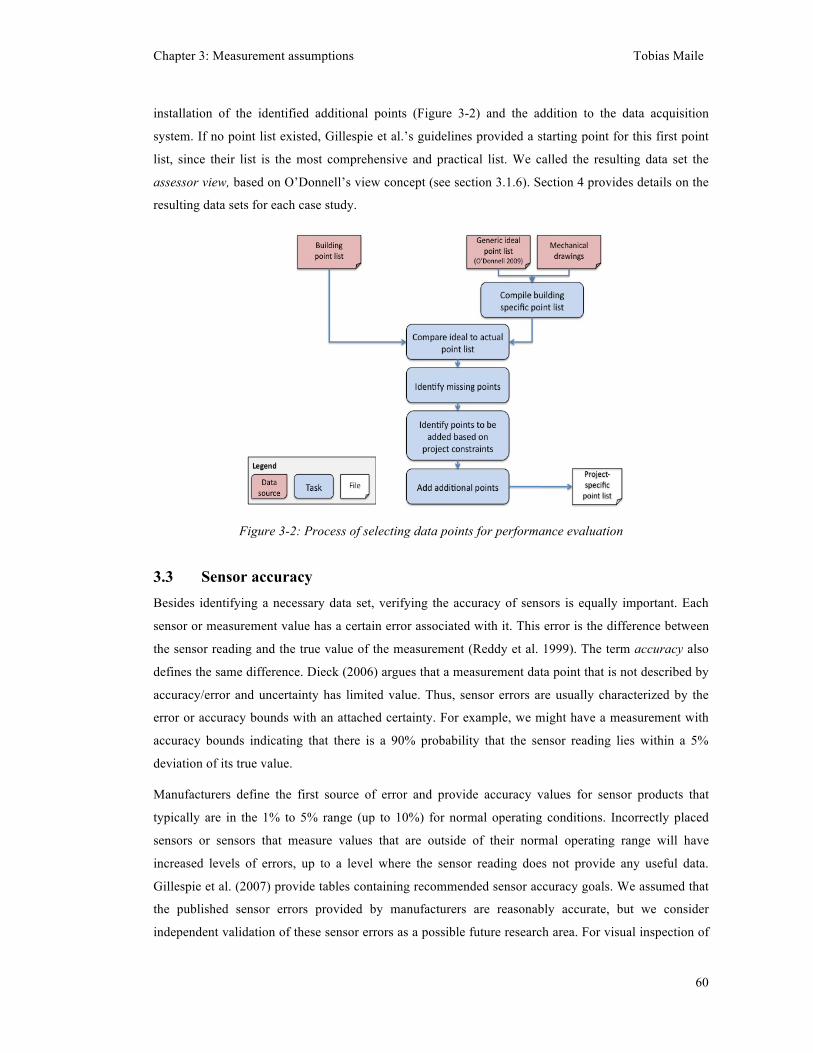
Chapter 3: Measurement assumptions Tobias Maile
60
installation of the identified additional points (Figure 3-2) and the addition to the data acquisition
system. If no point list existed, Gillespie et al.’s guidelines provided a starting point for this first point
list, since their list is the most comprehensive and practical list. We called the resulting data set the
assessor view, based on O’Donnell’s view concept (see section 3.1.6). Section 4 provides details on the
resulting data sets for each case study.
Figure 3-2: Process of selecting data points for performance evaluation
3.3 Sensor accuracy Besides identifying a necessary data set, verifying the accuracy of sensors is equally important. Each
sensor or measurement value has a certain error associated with it. This error is the difference between
the sensor reading and the true value of the measurement (Reddy et al. 1999). The term accuracy also
defines the same difference. Dieck (2006) argues that a measurement data point that is not described by
accuracy/error and uncertainty has limited value. Thus, sensor errors are usually characterized by the
error or accuracy bounds with an attached certainty. For example, we might have a measurement with
accuracy bounds indicating that there is a 90% probability that the sensor reading lies within a 5%
deviation of its true value.
Manufacturers define the first source of error and provide accuracy values for sensor products that
typically are in the 1% to 5% range (up to 10%) for normal operating conditions. Incorrectly placed
sensors or sensors that measure values that are outside of their normal operating range will have
increased levels of errors, up to a level where the sensor reading does not provide any useful data.
Gillespie et al. (2007) provide tables containing recommended sensor accuracy goals. We assumed that
the published sensor errors provided by manufacturers are reasonably accurate, but we consider
independent validation of these sensor errors as a possible future research area. For visual inspection of
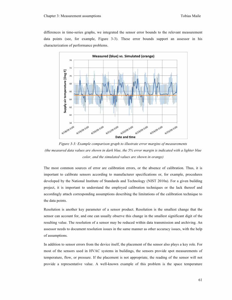
Chapter 3: Measurement assumptions Tobias Maile
61
differences in time-series graphs, we integrated the sensor error bounds to the relevant measurement
data points (see, for example, Figure 3-3). These error bounds support an assessor in his
characterization of performance problems.
Figure 3-3: Example comparison graph to illustrate error margins of measurements
(the measured data values are shown in dark blue, the 5% error margin is indicated with a lighter blue
color, and the simulated values are shown in orange)
The most common sources of error are calibration errors, or the absence of calibration. Thus, it is
important to calibrate sensors according to manufacturer specifications or, for example, procedures
developed by the National Institute of Standards and Technology (NIST 2010a). For a given building
project, it is important to understand the employed calibration techniques or the lack thereof and
accordingly attach corresponding assumptions describing the limitations of the calibration technique to
the data points.
Resolution is another key parameter of a sensor product. Resolution is the smallest change that the
sensor can account for, and one can usually observe this change in the smallest significant digit of the
resulting value. The resolution of a sensor may be reduced within data transmission and archiving. An
assessor needs to document resolution issues in the same manner as other accuracy issues, with the help
of assumptions.
In addition to sensor errors from the device itself, the placement of the sensor also plays a key role. For
most of the sensors used in HVAC systems in buildings, the sensors provide spot measurements of
temperature, flow, or pressure. If the placement is not appropriate, the reading of the sensor will not
provide a representative value. A well-known example of this problem is the space temperature
Chapter 3: Measurement assumptions Tobias Maile
62
measurement. This measurement typically resides within the space thermostat, which is usually located
next to one of the doors in a space. Avery (2002) illustrates a similar problem with mixed air
temperature measurements in air ducts. He argues that the resulting measurement result can be
inaccurate and influence the behavior of the system dramatically, even with multiple measurements that
are averaged. We refer to existing placement guidelines such as those provided by Klaassen (2001),
who specifically recommend placement guidelines for temperature sensors. ASHRAE (2007) provides
more generic and comprehensive guidelines for a wider range of sensor types.
In the context of a comparison with simulated data, errors of measurement have three key influences.
The first influence of measurement error is its relationship to assumptions. It is important to highlight
the limitations of sensors and document them as assumptions. These assumptions help one to
understand where differences between measurements and simulation results can originate. For example,
we encountered such a bottleneck in the form of the connection of the electrical sub-meters to the data
acquisition system, where multiple signal transformations led to numerous problems with our data.
Measurement assumptions are discussed in section 3.7. Since we used a set of measurements as input
for the updated simulation, the simulation results depend on the accuracy of the measurements. Maile et
al. (2010a) discuss the accuracy of simulation results. The second influence of measurement errors
occurs during the comparison process. If a measurement has a high error margin, the difference between
the measurement and simulation values becomes less important, and performance problems may be
hidden within the error margin.
3.4 Data transmission While the sensor defines the first level of accuracy and limitations, the transmission of data from the
sensor into storage may introduce additional shortcomings. A controller connects a number of sensors
as a part of the control system and may need to use some transformation to adjust for differences
between the sensor output signal and the controller input (typically analog to digital). The control
system exposes the controller input signal and allows corresponding data logger software to archive the
data. Through the use of additional data acquisition systems (such as specialized electrical sub-metering
systems), more transformation steps may be introduced and, therefore, more sources of errors may
exist. With each transformation step, the likelihood of errors increases. The use of different standards
and practices for measurements and data communication add to the problem of data transmission.
Typically, in a building, a number of different technologies and networks for measurements exist,
creating a need to integrate these different systems. A possible solution to problems of data
transmission in buildings is using an IP-based building system. If each sensor is directly integrated into
an IP-based network, only a single transformation is necessary (sensor signal to IP). Maile et al. (2007)
discuss this vision of IP-based building systems. In the context of a comparison with simulated data, it
Chapter 3: Measurement assumptions Tobias Maile
63
is important to understand these shortcomings of the data acquisition system and document them with
assumptions.
While the resolution of a sensor defines the basic resolution level, data transmission may decrease the
resolution level. If the right variable type is not assigned to a point within the control system, it may
dramatically change the resolution. Small changes in value stored in the smallest digit can get lost. For
example, a space temperature sensor normally has a resolution of a tenth of a degree; however, an
integer variable assigned to a temperature sensor value can change the resolution to one full degree. It is
common that control systems use integer variables for temperature measurements; however, these
values are multiplied by a factor of ten to retain the resolution level. Obviously, one needs to perform a
backwards conversion to return to the actual measured value. The resolution of the sensor and of the
data transmission needs to be documented and described with assumptions, in case limitations exist.
3.5 Data archiving Data archiving is the last step of a measurement system, storing data values and corresponding
timestamps. Each sensed value has a timestamp attached, which becomes another potential source of
error. Problems with these timestamps or biases, in time, will pose a limitation to sensor networks
where the relationships between sensors are of interest. To ensure the proper date and time on storage
servers and data logging hardware, it is beneficial to synchronize time based on a shared time source.
Standard practice is to use a Coordinated Universal Time (UTC) timestamp to circumvent problems
with daylight saving time changes (e.g., Olken et al. 1998). Limitations of data storage, in particular
with respect to timestamps, should be documented with assumptions. Our recommendations for the
design and functionality of data archiving are summarized in section 6.3.
3.6 Process of identifying performance problems with the knowledge of
measurement assumptions The previously described limitations of measurement systems in buildings are the reasons that specific
data points in a building may not match simulation results. To identify performance problems from
differences, we introduce the concept of measurement assumptions. Previous work has mentioned
project-specific measurement assumptions only sparsely (e.g., Salsbury and Diamond 2000) and has not
provided a process for assigning assumptions to building objects and data points.
The process for using assumptions to detect performance problems from differences between simulated
and measured data is illustrated in Figure 3-4. The starting point for this process is a data graph
containing the measured and simulated data values of the same variable. The first step is to detect
differences between the simulated and measured data. We use simple statistical variables, the root mean
squared error (RMSE) and the mean bias error (MBE), to detect differences. The RMSE gives an
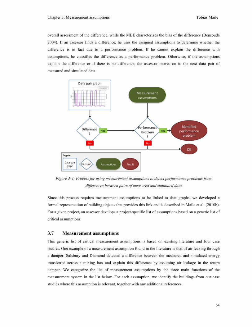
Chapter 3: Measurement assumptions Tobias Maile
64
overall assessment of the difference, while the MBE characterizes the bias of the difference (Bensouda
2004). If an assessor finds a difference, he uses the assigned assumptions to determine whether the
difference is in fact due to a performance problem. If he cannot explain the difference with
assumptions, he classifies the difference as a performance problem. Otherwise, if the assumptions
explain the difference or if there is no difference, the assessor moves on to the next data pair of
measured and simulated data.
Figure 3-4: Process for using measurement assumptions to detect performance problems from
differences between pairs of measured and simulated data
Since this process requires measurement assumptions to be linked to data graphs, we developed a
formal representation of building objects that provides this link and is described in Maile et al. (2010b).
For a given project, an assessor develops a project-specific list of assumptions based on a generic list of
critical assumptions.
3.7 Measurement assumptions This generic list of critical measurement assumptions is based on existing literature and four case
studies. One example of a measurement assumption found in the literature is that of air leaking through
a damper. Salsbury and Diamond detected a difference between the measured and simulated energy
transferred across a mixing box and explain this difference by assuming air leakage in the return
damper. We categorize the list of measurement assumptions by the three main functions of the
measurement system in the list below. For each assumption, we identify the buildings from our case
studies where this assumption is relevant, together with any additional references.
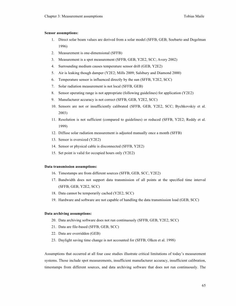
Chapter 3: Measurement assumptions Tobias Maile
65
Sensor assumptions:
1. Direct solar beam values are derived from a solar model (SFFB, GEB; Soebarto and Degelman
1996)
2. Measurement is one-dimensional (SFFB)
3. Measurement is a spot measurement (SFFB, GEB, Y2E2, SCC; Avery 2002)
4. Surrounding medium causes temperature sensor drift (GEB, Y2E2)
5. Air is leaking though damper (Y2E2; Mills 2009; Salsbury and Diamond 2000)
6. Temperature sensor is influenced directly by the sun (SFFB, Y2E2, SCC)
7. Solar radiation measurement is not local (SFFB, GEB)
8. Sensor operating range is not appropriate (following guidelines) for application (Y2E2)
9. Manufacturer accuracy is not correct (SFFB, GEB, Y2E2, SCC)
10. Sensors are not or insufficiently calibrated (SFFB, GEB, Y2E2, SCC; Bychkovskiy et al.
2003)
11. Resolution is not sufficient (compared to guidelines) or reduced (SFFB, Y2E2; Reddy et al.
1999)
12. Diffuse solar radiation measurement is adjusted manually once a month (SFFB)
13. Sensor is oversized (Y2E2)
14. Sensor or physical cable is disconnected (SFFB, Y2E2)
15. Set point is valid for occupied hours only (Y2E2)
Data transmission assumptions:
16. Timestamps are from different sources (SFFB, GEB, SCC, Y2E2)
17. Bandwidth does not support data transmission of all points at the specified time interval
(SFFB, GEB, Y2E2, SCC)
18. Data cannot be temporarily cached (Y2E2, SCC)
19. Hardware and software are not capable of handling the data transmission load (GEB, SCC)
Data archiving assumptions:
20. Data archiving software does not run continuously (SFFB, GEB, Y2E2, SCC)
21. Data are file-based (SFFB, GEB, SCC)
22. Data are overridden (GEB)
23. Daylight saving time change is not accounted for (SFFB; Olken et al. 1998)
Assumptions that occurred at all four case studies illustrate critical limitations of today’s measurement
systems. Those include spot measurements, insufficient manufacturer accuracy, insufficient calibration,
timestamps from different sources, and data archiving software that does not run continuously. The
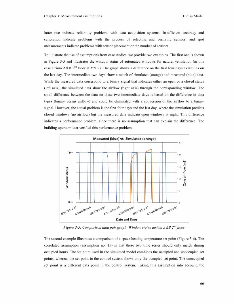
Chapter 3: Measurement assumptions Tobias Maile
66
latter two indicate reliability problems with data acquisition systems. Insufficient accuracy and
calibration indicate problems with the process of selecting and verifying sensors, and spot
measurements indicate problems with sensor placement or the number of sensors.
To illustrate the use of assumptions from case studies, we provide two examples. The first one is shown
in Figure 3-5 and illustrates the window status of automated windows for natural ventilation (in this
case atrium A&B 2nd floor at Y2E2). The graph shows a difference on the first four days as well as on
the last day. The intermediate two days show a match of simulated (orange) and measured (blue) data.
While the measured data correspond to a binary signal that indicates either an open or a closed status
(left axis), the simulated data show the airflow (right axis) through the corresponding window. The
small difference between the data on these two intermediate days is based on the difference in data
types (binary versus airflow) and could be eliminated with a conversion of the airflow to a binary
signal. However, the actual problem is the first four days and the last day, where the simulation predicts
closed windows (no airflow) but the measured data indicate open windows at night. This difference
indicates a performance problem, since there is no assumption that can explain the difference. The
building operator later verified this performance problem.
Figure 3-5: Comparison data pair graph: Window status atrium A&B 2nd floor
The second example illustrates a comparison of a space heating temperature set point (Figure 3-6). The
correlated assumption (assumption no. 15) is that these two time series should only match during
occupied hours. The set point used in the simulated model combines the occupied and unoccupied set
points, whereas the set point in the control system shows only the occupied set point. The unoccupied
set point is a different data point in the control system. Taking this assumption into account, the
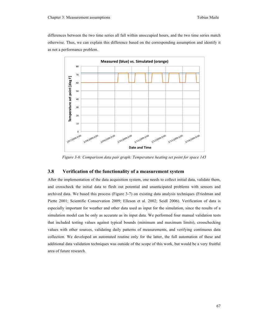
Chapter 3: Measurement assumptions Tobias Maile
67
differences between the two time series all fall within unoccupied hours, and the two time series match
otherwise. Thus, we can explain this difference based on the corresponding assumption and identify it
as not a performance problem.
Figure 3-6: Comparison data pair graph: Temperature heating set point for space 143
3.8 Verification of the functionality of a measurement system After the implementation of the data acquisition system, one needs to collect initial data, validate them,
and crosscheck the initial data to flesh out potential and unanticipated problems with sensors and
archived data. We based this process (Figure 3-7) on existing data analysis techniques (Friedman and
Piette 2001; Scientific Conservation 2009; Elleson et al. 2002; Seidl 2006). Verification of data is
especially important for weather and other data used as input for the simulation, since the results of a
simulation model can be only as accurate as its input data. We performed four manual validation tests
that included testing values against typical bounds (minimum and maximum limits), crosschecking
values with other sources, validating daily patterns of measurements, and verifying continuous data
collection. We developed an automated routine only for the latter, the full automation of these and
additional data validation techniques was outside of the scope of this work, but would be a very fruitful
area of future research.
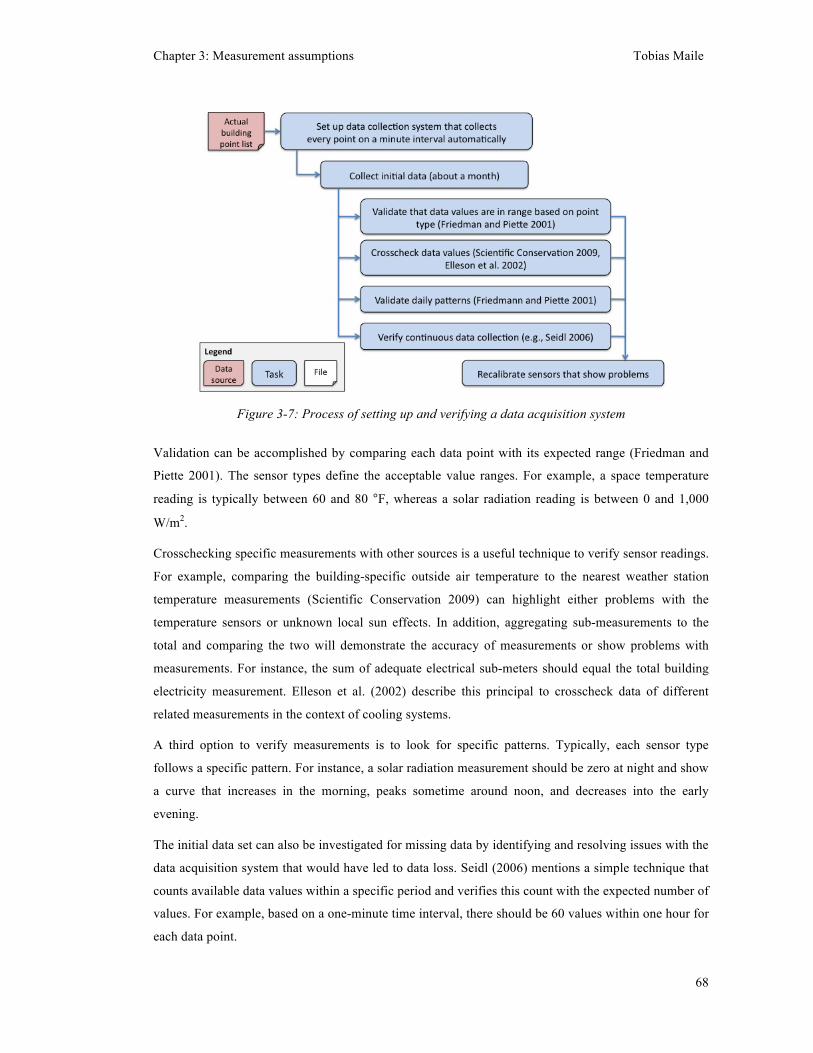
Chapter 3: Measurement assumptions Tobias Maile
68
Figure 3-7: Process of setting up and verifying a data acquisition system
Validation can be accomplished by comparing each data point with its expected range (Friedman and
Piette 2001). The sensor types define the acceptable value ranges. For example, a space temperature
reading is typically between 60 and 80 °F, whereas a solar radiation reading is between 0 and 1,000
W/m2.
Crosschecking specific measurements with other sources is a useful technique to verify sensor readings.
For example, comparing the building-specific outside air temperature to the nearest weather station
temperature measurements (Scientific Conservation 2009) can highlight either problems with the
temperature sensors or unknown local sun effects. In addition, aggregating sub-measurements to the
total and comparing the two will demonstrate the accuracy of measurements or show problems with
measurements. For instance, the sum of adequate electrical sub-meters should equal the total building
electricity measurement. Elleson et al. (2002) describe this principal to crosscheck data of different
related measurements in the context of cooling systems.
A third option to verify measurements is to look for specific patterns. Typically, each sensor type
follows a specific pattern. For instance, a solar radiation measurement should be zero at night and show
a curve that increases in the morning, peaks sometime around noon, and decreases into the early
evening.
The initial data set can also be investigated for missing data by identifying and resolving issues with the
data acquisition system that would have led to data loss. Seidl (2006) mentions a simple technique that
counts available data values within a specific period and verifies this count with the expected number of
values. For example, based on a one-minute time interval, there should be 60 values within one hour for
each data point.
Chapter 3: Measurement assumptions Tobias Maile
69
Based on the results of these validation techniques, one needs to recalibrate sensors that show problems.
Our focus for the manual validation of sensors was on weather and other input data for the simulation to
minimize the time effort and focus on the most important sensors. This manual verification process of
critical sensors took about half a day per case study. We automated the validation of the number of
archived data points per period to continuously control the reliability of archived data. Other automated
data validation techniques (e.g., Hou et al. 2006) require correct sensor readings to train algorithms and,
thus, are not useful for an initial data validation.
3.9 Reliability of a measurement system A data acquisition system needs to provide some level of reliability. We defined a reliability measure
that illustrates how many data values are present in the archive compared to the theoretical number of
data values (the reliability measure equals the number of actual archived data values divided by the
theoretical total number of data values for a given time interval and timeframe). We used this reliability
measure to compare the reliability of the data acquisition systems of the four case studies as shown in
section 4.6.
4 Case studies We chose four case studies to observe the current practice of measurement assumptions and limitations
of measurement systems. The case studies provide real-life context (Yin 2003) for these topics. Case
studies are commonly used in this research field, since surveys or questionnaires rely on the existence
of sufficient knowledge and standard use. Based on our observations with the first two case studies, we
developed concepts for measurement assumptions and a process to detect performance problems from
differences. The two later case studies were used to prospectively validate these concepts and compare
them to the methods used in practice to illustrate the power of our approach. In this section, we provide
a brief description of the case studies, details on the measurement data set, and information about the
data acquisition system. We also show example findings; for detailed validation results, please see
Maile et al. (2010b).
For each of the case studies, we provide a short general description of the building (including floor area,
location, and start of occupancy). We briefly describe the air conditioning strategy and special
characteristics of the building, as well as details about the measurement data set. All of the
measurement data sets of the four case studies are compared in Table 4 and put into the perspective of
existing measurement guidelines. We describe the data acquisition systems and highlight the advantages
and disadvantages of the particular setup. The selection process for these four case studies is described
in detail in Maile et al. (2010b). The four case studies have different HVAC systems and different usage
patterns to provide a range of buildings and HVAC systems that show the generality of our concepts.
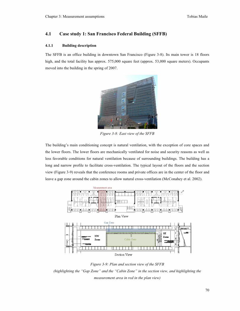
Chapter 3: Measurement assumptions Tobias Maile
70
4.1 Case study 1: San Francisco Federal Building (SFFB)
4.1.1 Building description
The SFFB is an office building in downtown San Francisco (Figure 3-8). Its main tower is 18 floors
high, and the total facility has approx. 575,000 square feet (approx. 53,000 square meters). Occupants
moved into the building in the spring of 2007.
Figure 3-8: East view of the SFFB
The building’s main conditioning concept is natural ventilation, with the exception of core spaces and
the lower floors. The lower floors are mechanically ventilated for noise and security reasons as well as
less favorable conditions for natural ventilation because of surrounding buildings. The building has a
long and narrow profile to facilitate cross-ventilation. The typical layout of the floors and the section
view (Figure 3-9) reveals that the conference rooms and private offices are in the center of the floor and
leave a gap zone around the cabin zones to allow natural cross-ventilation (McConahey et al. 2002).
Figure 3-9: Plan and section view of the SFFB
(highlighting the “Gap Zone” and the “Cabin Zone” in the section view, and highlighting the
measurement area in red in the plan view)
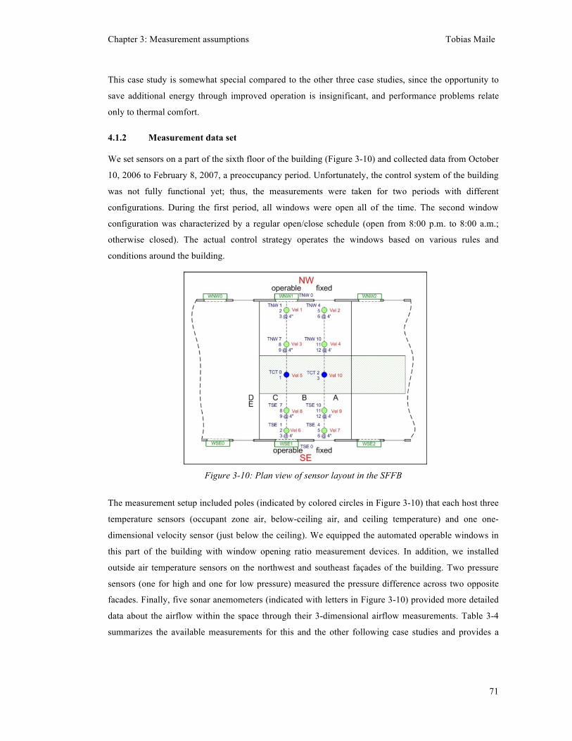
Chapter 3: Measurement assumptions Tobias Maile
71
This case study is somewhat special compared to the other three case studies, since the opportunity to
save additional energy through improved operation is insignificant, and performance problems relate
only to thermal comfort.
4.1.2 Measurement data set
We set sensors on a part of the sixth floor of the building (Figure 3-10) and collected data from October
10, 2006 to February 8, 2007, a preoccupancy period. Unfortunately, the control system of the building
was not fully functional yet; thus, the measurements were taken for two periods with different
configurations. During the first period, all windows were open all of the time. The second window
configuration was characterized by a regular open/close schedule (open from 8:00 p.m. to 8:00 a.m.;
otherwise closed). The actual control strategy operates the windows based on various rules and
conditions around the building.
Figure 3-10: Plan view of sensor layout in the SFFB
The measurement setup included poles (indicated by colored circles in Figure 3-10) that each host three
temperature sensors (occupant zone air, below-ceiling air, and ceiling temperature) and one one-
dimensional velocity sensor (just below the ceiling). We equipped the automated operable windows in
this part of the building with window opening ratio measurement devices. In addition, we installed
outside air temperature sensors on the northwest and southeast façades of the building. Two pressure
sensors (one for high and one for low pressure) measured the pressure difference across two opposite
facades. Finally, five sonar anemometers (indicated with letters in Figure 3-10) provided more detailed
data about the airflow within the space through their 3-dimensional airflow measurements. Table 3-4
summarizes the available measurements for this and the other following case studies and provides a
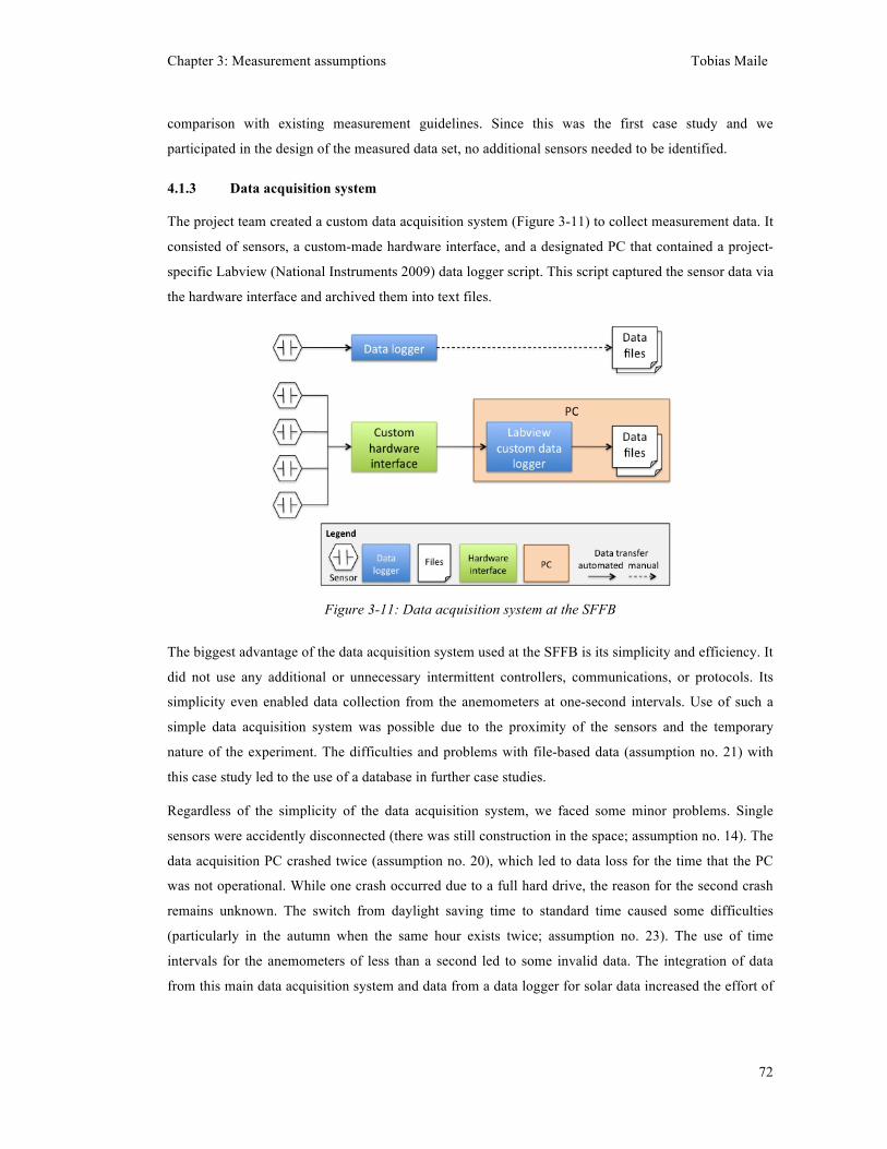
Chapter 3: Measurement assumptions Tobias Maile
72
comparison with existing measurement guidelines. Since this was the first case study and we
participated in the design of the measured data set, no additional sensors needed to be identified.
4.1.3 Data acquisition system
The project team created a custom data acquisition system (Figure 3-11) to collect measurement data. It
consisted of sensors, a custom-made hardware interface, and a designated PC that contained a project-
specific Labview (National Instruments 2009) data logger script. This script captured the sensor data via
the hardware interface and archived them into text files.
Figure 3-11: Data acquisition system at the SFFB
The biggest advantage of the data acquisition system used at the SFFB is its simplicity and efficiency. It
did not use any additional or unnecessary intermittent controllers, communications, or protocols. Its
simplicity even enabled data collection from the anemometers at one-second intervals. Use of such a
simple data acquisition system was possible due to the proximity of the sensors and the temporary
nature of the experiment. The difficulties and problems with file-based data (assumption no. 21) with
this case study led to the use of a database in further case studies.
Regardless of the simplicity of the data acquisition system, we faced some minor problems. Single
sensors were accidently disconnected (there was still construction in the space; assumption no. 14). The
data acquisition PC crashed twice (assumption no. 20), which led to data loss for the time that the PC
was not operational. While one crash occurred due to a full hard drive, the reason for the second crash
remains unknown. The switch from daylight saving time to standard time caused some difficulties
(particularly in the autumn when the same hour exists twice; assumption no. 23). The use of time
intervals for the anemometers of less than a second led to some invalid data. The integration of data
from this main data acquisition system and data from a data logger for solar data increased the effort of
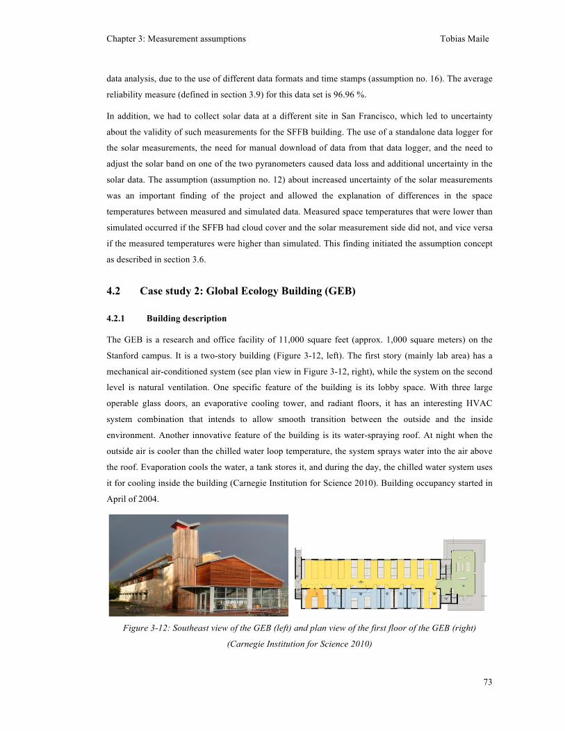
Chapter 3: Measurement assumptions Tobias Maile
73
data analysis, due to the use of different data formats and time stamps (assumption no. 16). The average
reliability measure (defined in section 3.9) for this data set is 96.96 %.
In addition, we had to collect solar data at a different site in San Francisco, which led to uncertainty
about the validity of such measurements for the SFFB building. The use of a standalone data logger for
the solar measurements, the need for manual download of data from that data logger, and the need to
adjust the solar band on one of the two pyranometers caused data loss and additional uncertainty in the
solar data. The assumption (assumption no. 12) about increased uncertainty of the solar measurements
was an important finding of the project and allowed the explanation of differences in the space
temperatures between measured and simulated data. Measured space temperatures that were lower than
simulated occurred if the SFFB had cloud cover and the solar measurement side did not, and vice versa
if the measured temperatures were higher than simulated. This finding initiated the assumption concept
as described in section 3.6.
4.2 Case study 2: Global Ecology Building (GEB)
4.2.1 Building description
The GEB is a research and office facility of 11,000 square feet (approx. 1,000 square meters) on the
Stanford campus. It is a two-story building (Figure 3-12, left). The first story (mainly lab area) has a
mechanical air-conditioned system (see plan view in Figure 3-12, right), while the system on the second
level is natural ventilation. One specific feature of the building is its lobby space. With three large
operable glass doors, an evaporative cooling tower, and radiant floors, it has an interesting HVAC
system combination that intends to allow smooth transition between the outside and the inside
environment. Another innovative feature of the building is its water-spraying roof. At night when the
outside air is cooler than the chilled water loop temperature, the system sprays water into the air above
the roof. Evaporation cools the water, a tank stores it, and during the day, the chilled water system uses
it for cooling inside the building (Carnegie Institution for Science 2010). Building occupancy started in
April of 2004.
Figure 3-12: Southeast view of the GEB (left) and plan view of the first floor of the GEB (right)
(Carnegie Institution for Science 2010)
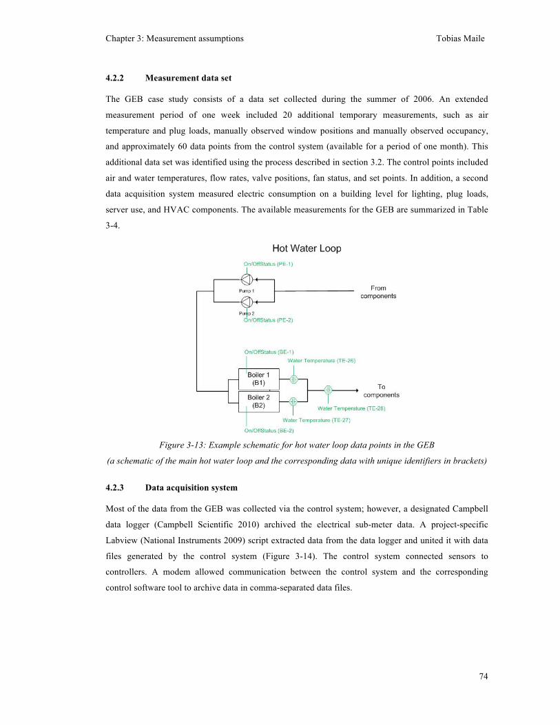
Chapter 3: Measurement assumptions Tobias Maile
74
4.2.2 Measurement data set
The GEB case study consists of a data set collected during the summer of 2006. An extended
measurement period of one week included 20 additional temporary measurements, such as air
temperature and plug loads, manually observed window positions and manually observed occupancy,
and approximately 60 data points from the control system (available for a period of one month). This
additional data set was identified using the process described in section 3.2. The control points included
air and water temperatures, flow rates, valve positions, fan status, and set points. In addition, a second
data acquisition system measured electric consumption on a building level for lighting, plug loads,
server use, and HVAC components. The available measurements for the GEB are summarized in Table
3-4.
Figure 3-13: Example schematic for hot water loop data points in the GEB
(a schematic of the main hot water loop and the corresponding data with unique identifiers in brackets)
4.2.3 Data acquisition system
Most of the data from the GEB was collected via the control system; however, a designated Campbell
data logger (Campbell Scientific 2010) archived the electrical sub-meter data. A project-specific
Labview (National Instruments 2009) script extracted data from the data logger and united it with data
files generated by the control system (Figure 3-14). The control system connected sensors to
controllers. A modem allowed communication between the control system and the corresponding
control software tool to archive data in comma-separated data files.
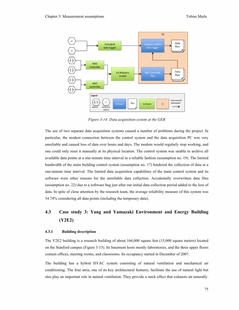
Chapter 3: Measurement assumptions Tobias Maile
75
Figure 3-14: Data acquisition system at the GEB
The use of two separate data acquisition systems caused a number of problems during the project. In
particular, the modem connection between the control system and the data acquisition PC was very
unreliable and caused loss of data over hours and days. The modem would regularly stop working, and
one could only reset it manually at its physical location. The control system was unable to archive all
available data points at a one-minute time interval in a reliable fashion (assumption no. 19). The limited
bandwidth of the main building control system (assumption no. 17) hindered the collection of data at a
one-minute time interval. The limited data acquisition capabilities of the main control system and its
software were other reasons for the unreliable data collection. Accidentally overwritten data files
(assumption no. 22) due to a software bug just after our initial data collection period added to the loss of
data. In spite of close attention by the research team, the average reliability measure of this system was
34.74% considering all data points (including the temporary data).
4.3 Case study 3: Yang and Yamazaki Environment and Energy Building
(Y2E2)
4.3.1 Building description
The Y2E2 building is a research building of about 166,000 square feet (15,000 square meters) located
on the Stanford campus (Figure 3-15). Its basement hosts mostly laboratories, and the three upper floors
contain offices, meeting rooms, and classrooms. Its occupancy started in December of 2007.
The building has a hybrid HVAC system consisting of natural ventilation and mechanical air
conditioning. The four atria, one of its key architectural features, facilitate the use of natural light but
also play an important role in natural ventilation. They provide a stack effect that exhausts air naturally.
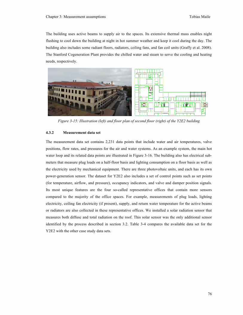
Chapter 3: Measurement assumptions Tobias Maile
76
The building uses active beams to supply air to the spaces. Its extensive thermal mass enables night
flushing to cool down the building at night in hot summer weather and keep it cool during the day. The
building also includes some radiant floors, radiators, ceiling fans, and fan coil units (Graffy et al. 2008).
The Stanford Cogeneration Plant provides the chilled water and steam to serve the cooling and heating
needs, respectively.
Figure 3-15: Illustration (left) and floor plan of second floor (right) of the Y2E2 building
4.3.2 Measurement data set
The measurement data set contains 2,231 data points that include water and air temperatures, valve
positions, flow rates, and pressures for the air and water systems. As an example system, the main hot
water loop and its related data points are illustrated in Figure 3-16. The building also has electrical sub-
meters that measure plug loads on a half-floor basis and lighting consumption on a floor basis as well as
the electricity used by mechanical equipment. There are three photovoltaic units, and each has its own
power-generation sensor. The dataset for Y2E2 also includes a set of control points such as set points
(for temperature, airflow, and pressure), occupancy indicators, and valve and damper position signals.
Its most unique features are the four so-called representative offices that contain more sensors
compared to the majority of the office spaces. For example, measurements of plug loads, lighting
electricity, ceiling fan electricity (if present), supply, and return water temperature for the active beams
or radiators are also collected in these representative offices. We installed a solar radiation sensor that
measures both diffuse and total radiation on the roof. This solar sensor was the only additional sensor
identified by the process described in section 3.2. Table 3-4 compares the available data set for the
Y2E2 with the other case study data sets.

Chapter 3: Measurement assumptions Tobias Maile
77
Figure 3-16: Example schematic for hot water loop data points in the Y2E2
(a schematic of the main hot water loop and the corresponding data points including unique identifiers
in brackets)(Haak et al. 2009)
4.3.3 Data acquisition system
The HVAC control system of the Y2E2 uses a LONwork’s protocol-based network (LonMark
International 2010) consisting of six subnets (Figure 3-17). The sensors communicate directly with the
controllers. The controllers, as part of one sub-network, connect to one iLON server (Echelon 2010).
Each iLON server has its own data logger that stores the data temporarily on the iLON server. A
Windows logging service connects to the iLON servers and fetches the available data from it via the
Ethernet. This logging service archives the received data into a MySQL database. We implemented this
setup since it was the only feasible solution to archive all sensor data at one-minute intervals. Since the
bandwidth of the control system was limited, the solution with an iLON server on each subnet enabled
us to reduce network traffic compared to using a solution in which all network traffic goes through one
interface.
The LONwork-based control system also integrates two additional systems. The campus-wide energy
management control system (EMCS) connects via a field server to the LONwork network. This EMCS
system controls the main systems in the building. Therefore, the sensors of the main systems are
integrated into the data acquisition system via the EMCS and field server. The iLON server also
integrates the electrical sub-meters directly via Modbus (Modbus 2009).
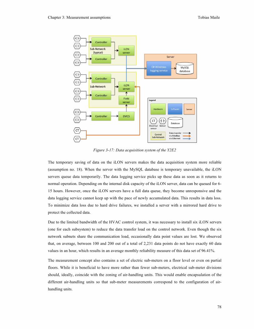
Chapter 3: Measurement assumptions Tobias Maile
78
Figure 3-17: Data acquisition system of the Y2E2
The temporary saving of data on the iLON servers makes the data acquisition system more reliable
(assumption no. 18). When the server with the MySQL database is temporary unavailable, the iLON
servers queue data temporarily. The data logging service picks up these data as soon as it returns to
normal operation. Depending on the internal disk capacity of the iLON server, data can be queued for 6-
15 hours. However, once the iLON servers have a full data queue, they become unresponsive and the
data logging service cannot keep up with the pace of newly accumulated data. This results in data loss.
To minimize data loss due to hard drive failures, we installed a server with a mirrored hard drive to
protect the collected data.
Due to the limited bandwidth of the HVAC control system, it was necessary to install six iLON servers
(one for each subsystem) to reduce the data transfer load on the control network. Even though the six
network subnets share the communication load, occasionally data point values are lost. We observed
that, on average, between 100 and 200 out of a total of 2,231 data points do not have exactly 60 data
values in an hour, which results in an average monthly reliability measure of this data set of 96.41%.
The measurement concept also contains a set of electric sub-meters on a floor level or even on partial
floors. While it is beneficial to have more rather than fewer sub-meters, electrical sub-meter divisions
should, ideally, coincide with the zoning of air-handling units. This would enable encapsulation of the
different air-handling units so that sub-meter measurements correspond to the configuration of air-
handling units.
Chapter 3: Measurement assumptions Tobias Maile
79
The control system configuration did not expose all sensor and control points automatically. We could
only expose points after understanding the architecture of the control network and the behavior of
different controller types within it. The actual implementation of this control system dramatically
increased the effort and difficulty of exposing points by several days. The controller inputs and outputs
of hardware and software did not correlate for some controllers. While it was possible to directly access
the hardware inputs and outputs and expose them for archiving, this workaround circumvented data
conversion routines within the control system. We had to reapply conversion routines within the
MySQL database.
In the Y2E2, the central university EMCS system connects to the control system, and several times;
someone accidently disconnected the physical connection (assumption no. 14). As a result, some data
were lost several times over multiple days. In addition, the connection between the electrical sub-meters
and the data acquisition system was so complex that it took over 24 months to identify and fix the
problems with electrical sub-metered data.
Another problem is that the water flow sensors for domestic water provide unrealistic (and inaccurate)
data because they are oversized (assumption no. 13). The same was true for the electric sub-meters for
the first two years because of numerous problems of the sensors and data transmission. New sensors
and improved data transmission resolved these problems. If the true measured value is not within the
typical operating ranges (assumption no. 8), the error of measurement grows large enough that the data
collected is not trustworthy.
4.4 Case study 4: Santa Clara County Building (SCC)
4.4.1 Building description
The SCC is a 10-story building (Figure 3-18) of approx. 350,000 square feet (32,500 square meters).
This correctional facility mainly houses cellblocks but also includes some office spaces and a kitchen.
The building is about 30 years old. It has a traditional mechanical HVAC system. Most air systems are
constant volume systems with 100% outside air. It has hot water boilers that serve the building’s
heating needs. Chiller and cooling towers provide the necessary cooling for the building.
We selected the building to be one of the case studies because it seemed to be relatively simple in terms
of its architecture, its HVAC systems, and its occupancy. The majority of floors have the same layout,
which simplifies the modeling of the geometry, even though it is the largest case study building. While
there have not been any dramatic changes to the building, the documentation in the form of drawings
and specifications is 30 years old and partially inconsistent. Compared to the other case studies, the
HVAC systems are very typical and relatively straightforward to model. Its occupancy is mostly
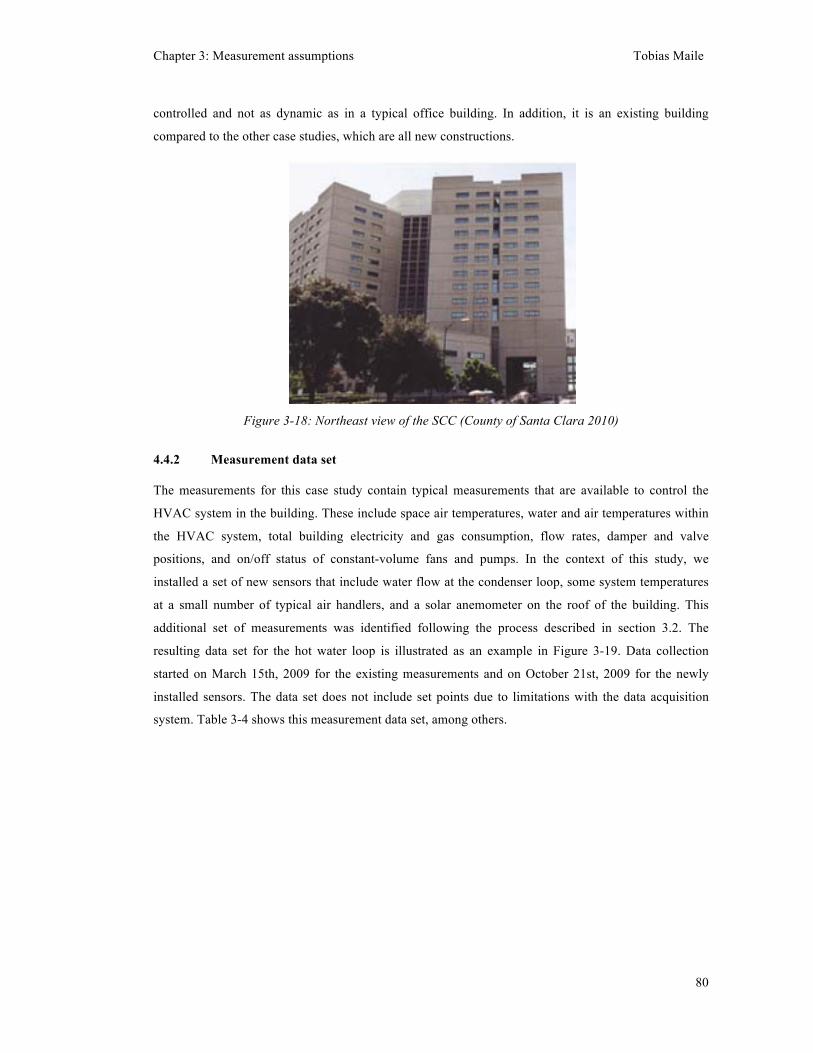
Chapter 3: Measurement assumptions Tobias Maile
80
controlled and not as dynamic as in a typical office building. In addition, it is an existing building
compared to the other case studies, which are all new constructions.
Figure 3-18: Northeast view of the SCC (County of Santa Clara 2010)
4.4.2 Measurement data set
The measurements for this case study contain typical measurements that are available to control the
HVAC system in the building. These include space air temperatures, water and air temperatures within
the HVAC system, total building electricity and gas consumption, flow rates, damper and valve
positions, and on/off status of constant-volume fans and pumps. In the context of this study, we
installed a set of new sensors that include water flow at the condenser loop, some system temperatures
at a small number of typical air handlers, and a solar anemometer on the roof of the building. This
additional set of measurements was identified following the process described in section 3.2. The
resulting data set for the hot water loop is illustrated as an example in Figure 3-19. Data collection
started on March 15th, 2009 for the existing measurements and on October 21st, 2009 for the newly
installed sensors. The data set does not include set points due to limitations with the data acquisition
system. Table 3-4 shows this measurement data set, among others.
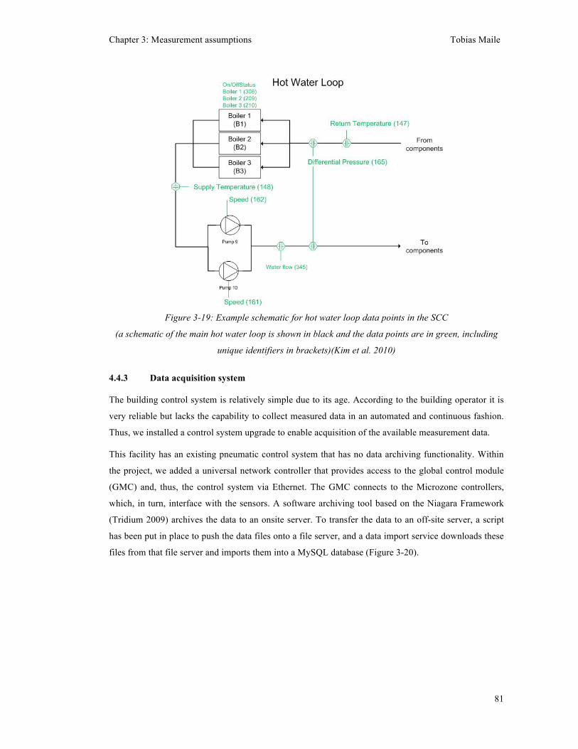
Chapter 3: Measurement assumptions Tobias Maile
81
Figure 3-19: Example schematic for hot water loop data points in the SCC
(a schematic of the main hot water loop is shown in black and the data points are in green, including
unique identifiers in brackets)(Kim et al. 2010)
4.4.3 Data acquisition system
The building control system is relatively simple due to its age. According to the building operator it is
very reliable but lacks the capability to collect measured data in an automated and continuous fashion.
Thus, we installed a control system upgrade to enable acquisition of the available measurement data.
This facility has an existing pneumatic control system that has no data archiving functionality. Within
the project, we added a universal network controller that provides access to the global control module
(GMC) and, thus, the control system via Ethernet. The GMC connects to the Microzone controllers,
which, in turn, interface with the sensors. A software archiving tool based on the Niagara Framework
(Tridium 2009) archives the data to an onsite server. To transfer the data to an off-site server, a script
has been put in place to push the data files onto a file server, and a data import service downloads these
files from that file server and imports them into a MySQL database (Figure 3-20).
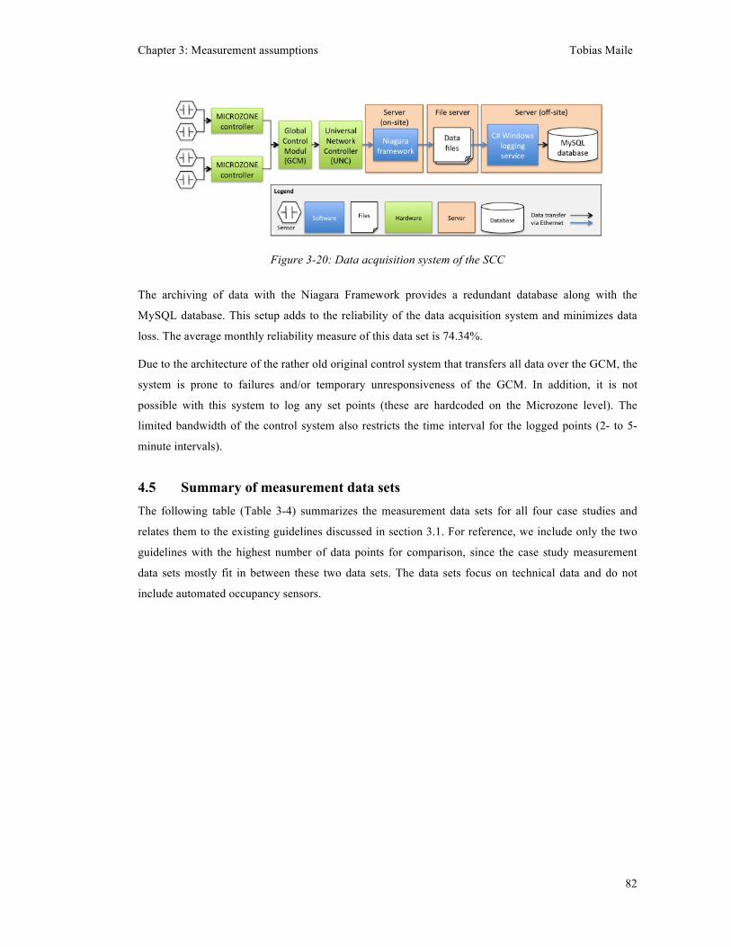
Chapter 3: Measurement assumptions Tobias Maile
82
Figure 3-20: Data acquisition system of the SCC
The archiving of data with the Niagara Framework provides a redundant database along with the
MySQL database. This setup adds to the reliability of the data acquisition system and minimizes data
loss. The average monthly reliability measure of this data set is 74.34%.
Due to the architecture of the rather old original control system that transfers all data over the GCM, the
system is prone to failures and/or temporary unresponsiveness of the GCM. In addition, it is not
possible with this system to log any set points (these are hardcoded on the Microzone level). The
limited bandwidth of the control system also restricts the time interval for the logged points (2- to 5-
minute intervals).
4.5 Summary of measurement data sets The following table (Table 3-4) summarizes the measurement data sets for all four case studies and
relates them to the existing guidelines discussed in section 3.1. For reference, we include only the two
guidelines with the highest number of data points for comparison, since the case study measurement
data sets mostly fit in between these two data sets. The data sets focus on technical data and do not
include automated occupancy sensors.
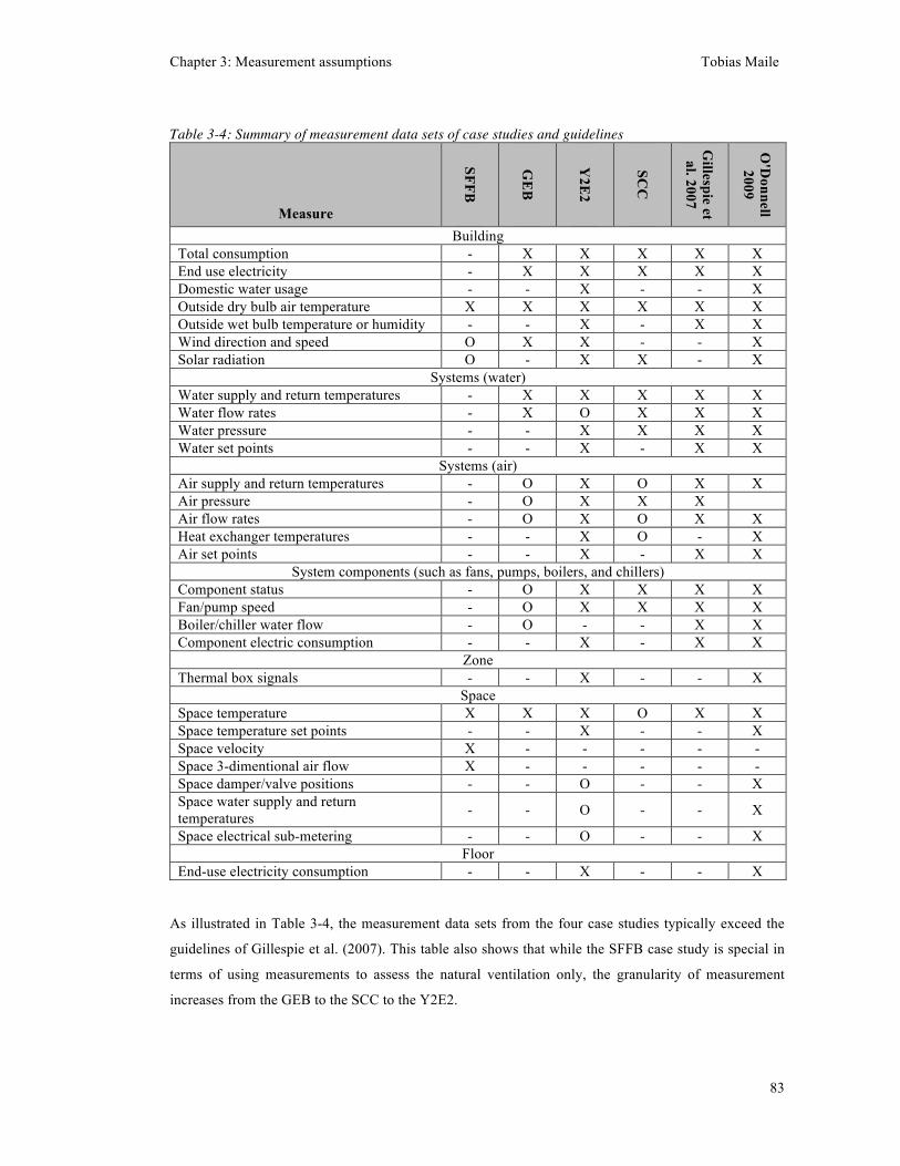
Chapter 3: Measurement assumptions Tobias Maile
83
Table 3-4: Summary of measurement data sets of case studies and guidelines
Measure
SFFB
GE
B
Y2E
2
SCC
Gillespie et al. 2007
O'D
onnell 2009
Building Total consumption - X X X X X End use electricity - X X X X X Domestic water usage - - X - - X Outside dry bulb air temperature X X X X X X Outside wet bulb temperature or humidity - - X - X X Wind direction and speed O X X - - X Solar radiation O - X X - X
Systems (water) Water supply and return temperatures - X X X X X Water flow rates - X O X X X Water pressure - - X X X X Water set points - - X - X X
Systems (air) Air supply and return temperatures - O X O X X Air pressure - O X X X Air flow rates - O X O X X Heat exchanger temperatures - - X O - X Air set points - - X - X X
System components (such as fans, pumps, boilers, and chillers) Component status - O X X X X Fan/pump speed - O X X X X Boiler/chiller water flow - O - - X X Component electric consumption - - X - X X
Zone Thermal box signals - - X - - X
Space Space temperature X X X O X X Space temperature set points - - X - - X Space velocity X - - - - - Space 3-dimentional air flow X - - - - - Space damper/valve positions - - O - - X Space water supply and return temperatures - - O - - X
Space electrical sub-metering - - O - - X Floor
End-use electricity consumption - - X - - X
As illustrated in Table 3-4, the measurement data sets from the four case studies typically exceed the
guidelines of Gillespie et al. (2007). This table also shows that while the SFFB case study is special in
terms of using measurements to assess the natural ventilation only, the granularity of measurement
increases from the GEB to the SCC to the Y2E2.
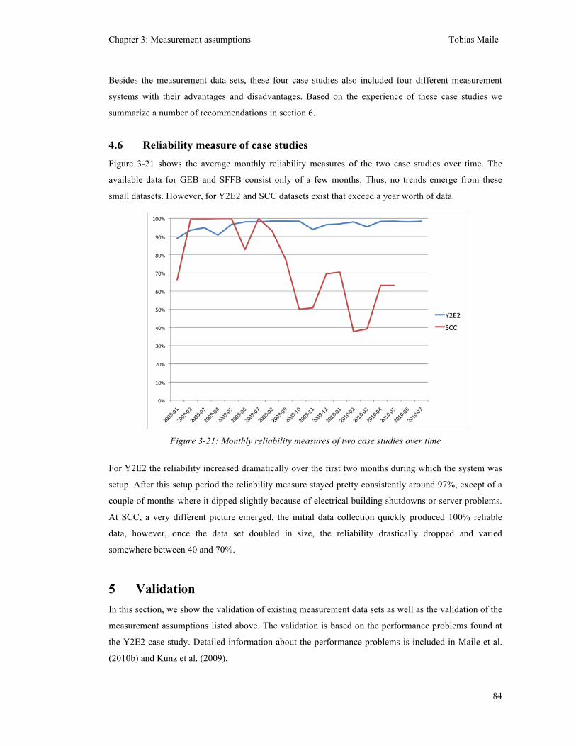
Chapter 3: Measurement assumptions Tobias Maile
84
Besides the measurement data sets, these four case studies also included four different measurement
systems with their advantages and disadvantages. Based on the experience of these case studies we
summarize a number of recommendations in section 6.
4.6 Reliability measure of case studies Figure 3-21 shows the average monthly reliability measures of the two case studies over time. The
available data for GEB and SFFB consist only of a few months. Thus, no trends emerge from these
small datasets. However, for Y2E2 and SCC datasets exist that exceed a year worth of data.
Figure 3-21: Monthly reliability measures of two case studies over time
For Y2E2 the reliability increased dramatically over the first two months during which the system was
setup. After this setup period the reliability measure stayed pretty consistently around 97%, except of a
couple of months where it dipped slightly because of electrical building shutdowns or server problems.
At SCC, a very different picture emerged, the initial data collection quickly produced 100% reliable
data, however, once the data set doubled in size, the reliability drastically dropped and varied
somewhere between 40 and 70%.
5 Validation In this section, we show the validation of existing measurement data sets as well as the validation of the
measurement assumptions listed above. The validation is based on the performance problems found at
the Y2E2 case study. Detailed information about the performance problems is included in Maile et al.
(2010b) and Kunz et al. (2009).
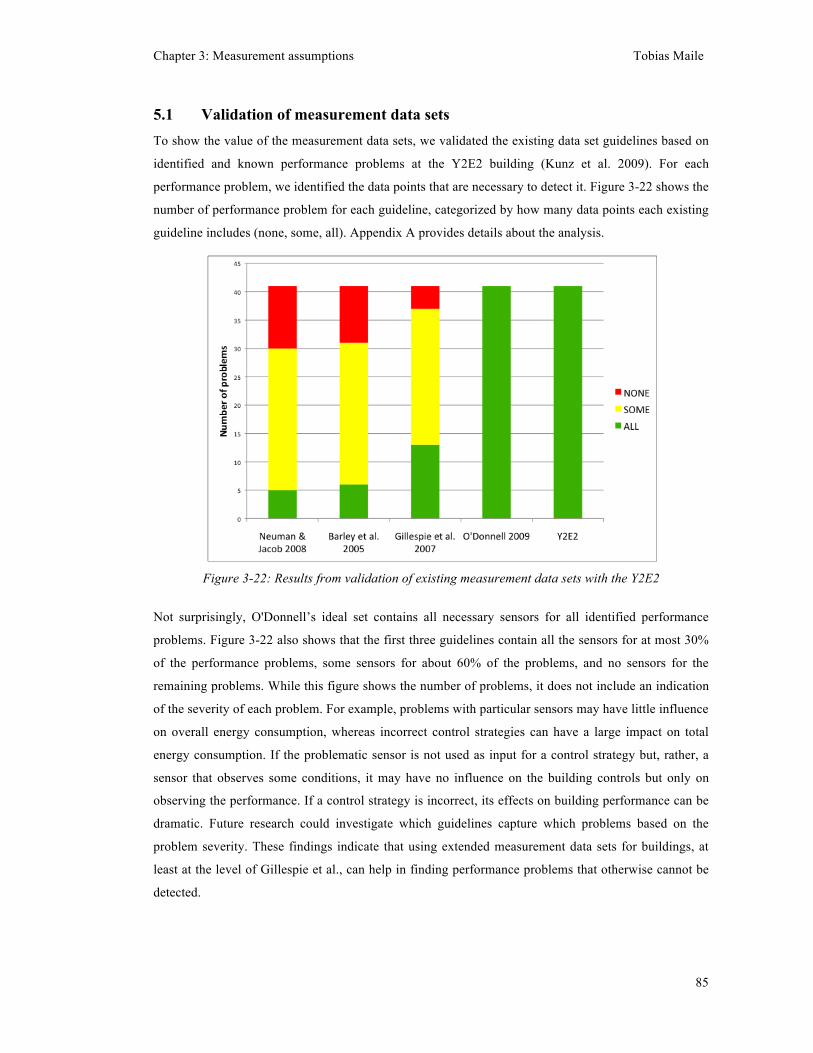
Chapter 3: Measurement assumptions Tobias Maile
85
5.1 Validation of measurement data sets To show the value of the measurement data sets, we validated the existing data set guidelines based on
identified and known performance problems at the Y2E2 building (Kunz et al. 2009). For each
performance problem, we identified the data points that are necessary to detect it. Figure 3-22 shows the
number of performance problem for each guideline, categorized by how many data points each existing
guideline includes (none, some, all). Appendix A provides details about the analysis.
Figure 3-22: Results from validation of existing measurement data sets with the Y2E2
Not surprisingly, O'Donnell’s ideal set contains all necessary sensors for all identified performance
problems. Figure 3-22 also shows that the first three guidelines contain all the sensors for at most 30%
of the performance problems, some sensors for about 60% of the problems, and no sensors for the
remaining problems. While this figure shows the number of problems, it does not include an indication
of the severity of each problem. For example, problems with particular sensors may have little influence
on overall energy consumption, whereas incorrect control strategies can have a large impact on total
energy consumption. If the problematic sensor is not used as input for a control strategy but, rather, a
sensor that observes some conditions, it may have no influence on the building controls but only on
observing the performance. If a control strategy is incorrect, its effects on building performance can be
dramatic. Future research could investigate which guidelines capture which problems based on the
problem severity. These findings indicate that using extended measurement data sets for buildings, at
least at the level of Gillespie et al., can help in finding performance problems that otherwise cannot be
detected.
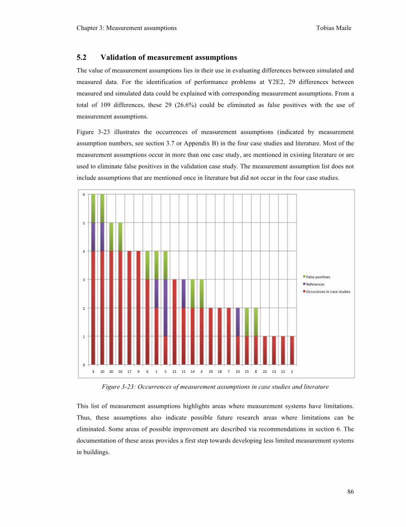
Chapter 3: Measurement assumptions Tobias Maile
86
5.2 Validation of measurement assumptions The value of measurement assumptions lies in their use in evaluating differences between simulated and
measured data. For the identification of performance problems at Y2E2, 29 differences between
measured and simulated data could be explained with corresponding measurement assumptions. From a
total of 109 differences, these 29 (26.6%) could be eliminated as false positives with the use of
measurement assumptions.
Figure 3-23 illustrates the occurrences of measurement assumptions (indicated by measurement
assumption numbers, see section 3.7 or Appendix B) in the four case studies and literature. Most of the
measurement assumptions occur in more than one case study, are mentioned in existing literature or are
used to eliminate false positives in the validation case study. The measurement assumption list does not
include assumptions that are mentioned once in literature but did not occur in the four case studies.
Figure 3-23: Occurrences of measurement assumptions in case studies and literature
This list of measurement assumptions highlights areas where measurement systems have limitations.
Thus, these assumptions also indicate possible future research areas where limitations can be
eliminated. Some areas of possible improvement are described via recommendations in section 6. The
documentation of these areas provides a first step towards developing less limited measurement systems
in buildings.
Chapter 3: Measurement assumptions Tobias Maile
87
6 Recommendations This section summarizes our recommendations based on the limitations of the measurement systems we
encountered during the case studies. These recommendations aim to improve the quality and
consistency of measurement systems by using existing measurement guidelines, calibrating sensors
more thoroughly, improving data archiving, and using local solar measurements.
6.1 Select appropriate sensors based on existing measurement guidelines The quality of data starts with the sensor products. While a number of guidelines and protocols exist
(e.g., Gillespie et al. 2007; Barley et al. 2005), our experience indicates that these guidelines are not
used to design data acquisition systems and to select appropriate sensor products. The accuracy,
resolution, and operating range of sensor products are key metrics that designers need to consider
during the process of planning data acquisition systems. It is important to select sensors of the right size
that reflect the anticipated flow or electrical loads, rather than a size based on the worst-case scenario
(see section 4.3.3). If the actual flow is difficult to estimate during design or varies dramatically during
measurement, one can install two sensors with different operating ranges that provide accurate readings
over an extended data scale. We used this concept at the SFFB (see section 4.1.2) for differential
pressure measurements. Thus, we recommend the use of existing guidelines to develop measurement
data sets.
6.2 Use more thorough sensor calibration We found several indications that sensor calibration is insufficient in practice during commissioning
and operation. The only case study where sensors were calibrated regularly was the SFFB case study,
where the solar sensor shading band needed adjustment once per month and the pressure sensor was
calibrated once per month. The insufficient calibration is illustrated by one example where we found
that the electrical sub-meters were off by a factor of eight after these sensors had been operating for
about a year. Any performed calibration effort should have identified this difference. Thus, we
recommend that sensor calibration needs to be more thorough during the commissioning or operation
phase of the building.
6.3 Design control systems that support continuous data archiving For the three case studies (except for the custom solution needed at SFFB), we used an existing control
system as the basis for data collection. It became apparent that those control systems, including
hardware, software, bandwidth, and interfaces, are not well suited for continuous and reliable data
collection of all data points at one-minute intervals. Various studies (Brambley et al. 2005; Torcellini et
al. 2006; O'Donnell 2009) report similar problems with data collection.
Chapter 3: Measurement assumptions Tobias Maile
88
Bandwidth limits were a problem in all three control systems. The lack of bandwidth made it difficult to
accommodate the communication necessary to archive all measurements on a one-minute basis. This
bandwidth problem is clearly an issue that originates in the control system design. The effort to increase
bandwidth at the design stage is minimal compared to that of retrofitting a building control system to
increase the bandwidth (e.g., at Y2E2 the costs of initially increasing the bandwidth from 78 kbit/s to
1.2 Mbit/s for the subnets and 1.2 Mbit/s to 100 Mbit/s for the backbone would have been several
thousand dollars, but the retrofit costs totaled several hundreds thousand dollars). The latter is a major
remodeling effort due to the need for rewiring.
Additionally, we encountered a number of problems with installed hardware that provided significant
limitations or led to data loss. For example, the modem at the GEB limited the data collection quite
dramatically (see section 4.2.3). Other examples include the iLON server’s inability to respond to
requests while having full data queues (see section 4.3.3) or the use of various sensor products that did
not perform as needed. The data storage capacity is another example of hardware limitations. We
encountered problems with exceeding storage capacities and data loss due to overridden data files.
A range of software limitations and problems reduced the reliability of the data collection. Instability of
operating systems (e.g., see section 4.1.3) and unresponsiveness of controller and iLON server software
led to data losses. In addition, limitations in the functionality of data collection software increased our
efforts to configure these systems and created a need for additional software development.
Another problem with the data acquisition systems is the interface between different types of control
systems. We encountered interface problems with two case studies, as described in the previous
sections (4.2.3 and 4.3.3). While communication between different control systems is needed to allow
for a central data acquisition system, it is important that integrating these systems does not reduce the
quality and reliability of data. For example, to ensure the data acquisition of set points and other control
variables, one should integrate data acquisition systems with the control systems. A missing integration
leads to the use of separate systems to archive data with corresponding challenges to synchronize the
data. A tight integration of the control system with the data acquisition system also allows better
understanding of the control system (Torcellini et al. 2006). A completely separate data acquisition
system may not be able to archive existing sensor and control signal data.
These bandwidth, hardware, software, and interface limitations create an environment in which reliable
continuous data collection is hard to achieve. Torcellini et al. (2006) report similar problems with the
reliability of data archiving with control systems. Thus, we recommend increasing the bandwidth of
control systems early in design to eliminate later problems with data acquisition, as well as selecting
appropriate data acquisition software that is capable of archiving all data points at one-minute intervals.
Data should be archived in a common database format with at least a timestamp and value for each
sensor reading. While current control systems have significant shortcomings in archiving data in an
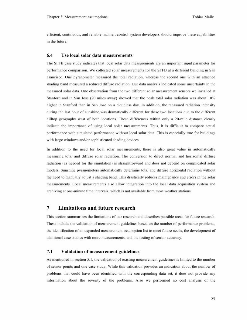
Chapter 3: Measurement assumptions Tobias Maile
89
efficient, continuous, and reliable manner, control system developers should improve these capabilities
in the future.
6.4 Use local solar data measurements The SFFB case study indicates that local solar data measurements are an important input parameter for
performance comparison. We collected solar measurements for the SFFB at a different building in San
Francisco. One pyranometer measured the total radiation, whereas the second one with an attached
shading band measured a reduced diffuse radiation. Our data analysis indicated some uncertainty in the
measured solar data. One observation from the two different solar measurement sensors we installed at
Stanford and in San Jose (20 miles away) showed that the peak total solar radiation was about 10%
higher in Stanford than in San Jose on a cloudless day. In addition, the measured radiation intensity
during the last hour of sunshine was dramatically different for these two locations due to the different
hilltop geography west of both locations. These differences within only a 20-mile distance clearly
indicate the importance of using local solar measurements. Thus, it is difficult to compare actual
performance with simulated performance without local solar data. This is especially true for buildings
with large windows and/or sophisticated shading devices.
In addition to the need for local solar measurements, there is also great value in automatically
measuring total and diffuse solar radiation. The conversion to direct normal and horizontal diffuse
radiation (as needed for the simulation) is straightforward and does not depend on complicated solar
models. Sunshine pyranometers automatically determine total and diffuse horizontal radiation without
the need to manually adjust a shading band. This drastically reduces maintenance and errors in the solar
measurements. Local measurements also allow integration into the local data acquisition system and
archiving at one-minute time intervals, which is not available from most weather stations.
7 Limitations and future research This section summarizes the limitations of our research and describes possible areas for future research.
These include the validation of measurement guidelines based on the number of performance problems,
the identification of an expanded measurement assumption list to meet future needs, the development of
additional case studies with more measurements, and the testing of sensor accuracy.
7.1 Validation of measurement guidelines As mentioned in section 5.1, the validation of existing measurement guidelines is limited to the number
of sensor points and one case study. While this validation provides an indication about the number of
problems that could have been identified with the corresponding data set, it does not provide any
information about the severity of the problems. Also we performed no cost analysis of the
Chapter 3: Measurement assumptions Tobias Maile
90
corresponding sensors and did not associate costs with specific problems. A fruitful future research area
is the validation of the measurement data sets using additional case studies with more focus on the
severity and cost of specific problems. With the severity of performance problems and costs of each
sensor a cost benefit analysis is possible to identify the actual value of a sensor. With more data on
actual performance problems in buildings, the cost benefit analysis and likelihood of a given problem
would provide a well-founded quantitative assessment of the need for particular sensors.
7.2 Identification of an expanded assumption list The list of assumptions (see section 3.7) is based on a literature review and the four case studies. Future
case studies and research may identify more assumptions. The development of new HVAC components,
systems, control strategies, data acquisition systems, and sensors may eliminate the need for some
measurement assumptions as well as create a need for additional measurement assumptions. While the
list of measurement assumptions is likely to change in the future due to the mentioned reasons, the
related processes will still be the same.
7.3 Development of case studies with more measurements While the four mentioned case studies have extended measurements above the typical level, future
research could use additional case studies that use even more measurement data points. With sensors
becoming more affordable and buildings more complex, additional sensors may provide additional
value for performance evaluation. In particular, occupancy sensors or dimming and luminance sensors
(via the lighting control system) may provide additional information regarding performance problems in
a building. Specifically, more measurements that provide more details about the usage of the building
such as occupant counts and window and door positions, would help eliminate some of the unknowns in
buildings. Without installing, testing and analyzing additional measurements the value and usefulness
of additional measurements may never be known. Thus, case studies that exceed the sensor level of the
four mentioned case studies could result in more insights about measuring and analyzing building
energy performance.
7.4 Testing of manufacturer accuracy of sensors As mentioned in section 3.3, we did not question the accuracy of sensors as provided by the
manufacturers. Future research could test the validity of claimed sensor accuracy. For example, a
ongoing research project at NIST focuses on the issue of sensor accuracy for commissioning and fault
detection of HVAC systems (NIST 2010b).
Chapter 3: Measurement assumptions Tobias Maile
91
8 Conclusion The two contributions of this paper are the list of critical measurement assumptions and the comparison
and validation of existing guidelines for measurement data sets. Measurement assumptions document
limitations of measurement systems according to their three functions (sensing, transmitting, and
archiving) and can support the assessor in evaluating the quality of measured data. We compiled a list
of critical measurement assumptions, categorized these measurement assumptions according to the
three functions of the measurement system, and developed a process to determine performance
problems from differences between simulated and measured data. This measurement assumption
concept allowed us to deal successfully with limitations we encountered with measurement systems in
the four case studies. These measurement assumptions are crucial for assessing measured data and
understanding the difference between measured data and the energy performance of the actual building.
The limitations of measurement systems start with the data set of sensors and control points; thus, we
compared and validated existing measurement data set guidelines and showed the value of using
additional sensors beyond those recommended in guidelines from Gillespie et al. (2007) or Barley et al.
(2005). We provided an overview and summary of existing guidelines for measurement data sets,
compared them to data sets of the case studies, and validated the data sets based on the known
performance problems of one case study. The results indicated that even extended measurement data
sets did not capture all sensors that were needed to identify our known set of performance problems.
Based on the results, we recommend designing measurement systems at least on the level of detail that
Gillespie et al. (2007) describe. Additionally, we recommend paying more attention to possible
limitations of measurement systems to decrease limitations and increase the quality of data. Particular
conclusions from the case studies include the need for local solar measurements due to possible
variations of local climates. We also learned that a key parameter of sensors is their operating range,
which can dramatically reduce the quality of the resulting data if it is not correct.
Based on these limitations of measurement systems, we found it difficult to achieve high reliability in a
measurement system. Even with upgraded data acquisition systems, the best achievement in terms of
average monthly reliability was about 97% of data at one-minute intervals over a time period of 15
months. We see large potential for improvement of data acquisition systems in the future to enable a
smoother analysis of measured data.
9 Bibliography ASHRAE. (2003). HVAC applications handbook. Atlanta, GA: ASHRAE Publications.

Chapter 3: Measurement assumptions Tobias Maile
92
ASHRAE. (2007). 2007 ASHRAE handbook - Heating, ventilating, and air-conditioning applications
(I-P edition). Atlanta, GA: American Society of Heating, Refrigerating and Air-Conditioning
Engineers, Inc.
Avery, G. (2002). Do averaging sensors average? ASHRAE Journal, 44(12), 42–43.
Barley, D., M. Deru, S. Pless, and P. Torcellini. (2005). Procedure for measuring and reporting
commercial building energy performance. Technical Report #550. Golden, CO: National
Renewable Energy Laboratory.
Bensouda, N. (2004). Extending and formalizing the energy signature method for calibrating
simulations and illustrating with application for three California climates. Master Thesis,
College Station, TX: Texas A&M University.
Brambley, M., D. Hansen, P. Haves, D. Holmberg, S. McDonald, K. Roth, and P. Torcellini. (2005).
Advanced sensors and controls for building applications: Market assessment and potential R
& D pathways. Prepared for the U.S. Department of Energy under Contract DE-AC05-
76RL01830. http://apps1.eere.energy.gov/buildings/publications/pdfs/corporate/pnnl-
15149_market_assessment.pdf last accessed on March 13, 2010.
Bychkovskiy, V., S. Megerian, D. Estrin, and M. Potkonjak. (2003). A collaborative approach to in-
place sensor calibration. Lecture Notes in Computer Science, 2634, 301–316.
Campbell Scientific. (2010). Campbell Scientific: Dataloggers, data acquisition systems, weather
stations. http://www.campbellsci.com/ last accessed on March 15, 2010.
Carnegie Institution for Science. (2010). Carnegie Department of Global Ecology.
http://dge.stanford.edu/about/building/ last accessed on March 15, 2010.
County of Santa Clara. (2010). Main Jail Complex - Correction, Department of (DEP).
http://www.sccgov.org/portal/site/doc last accessed on March 16, 2010.
Dieck, R. H. 2006. Measurement uncertainty: methods and applications. ISA - The Instrumentation,
Systems and Automation Society.
Echelon. 2010. i.LON SmarServer - Smart Energy Managers. http://www.echelon.com/products/cis/.
Elleson, J.S., J.S. Haberl, and T.A. Reddy. 2002. Field Monitoring and Data Validation for Evaluating
the Performance of Cool Storage Systems. In ASHRAE Transactions, 108:1072-1084. Vol.
108. 1. Atlantic City, NY.
Friedman, H., and M.A. Piette. 2001. Comparison of Emerging Diagnostic Tools for Large Commercial
HVAC Systems. Proceedings of the 7th National Conference on Building Commissioning. 1-
13. Cherry Hill, New Jersey: Portland Energy Conservation Inc (PECI).

Chapter 3: Measurement assumptions Tobias Maile
93
Gillespie, K.L., P. Haves, R.J. Hitchcock, J.J. Deringer, and K. Kinney. 2007. A Specifications Guide
for Performance Monitoring Systems. Berkeley, CA.
Graffy, K., J. Lidstone, C. Roberts, B.G. Sprague, J. Wayne, and A. Wolski. (2008). Y2E2: The Jerry
Yang and Akiko Yamazaki Environment and Energy Building, Stanford University,
California. The Arup Journal, 3, 44-55.
Haak, T., K. Megna, and T. Maile. (2009). Data manual of Stanford University’s Yang and Yamazaki
Environment & Energy Building. Internal document. Stanford, CA: Stanford University.
Hou, Zhijian, Zhiwei Lian, Ye Yao, and Xinjian Yuan. 2006. Data mining based sensor fault diagnosis
and validation for building air conditioning system. Energy Conversion and Management 47,
no. 15-16 (September): 2479-2490. doi:10.1016/j.enconman.2005.11.010.
Kim, M.J., K. Megna, and T. Maile. (2010). Data manual of Santa Clara County Main Jail North.
Internal document. Stanford, CA: Stanford University.
Klaassen, C.J. 2001. Installing BAS sensors properly. HPAC Engineering (August): 53-55.
Kunz, J., T. Maile, and V. Bazjanac. 2009. Summary of the Energy Analysis of the First Year of the
Stanford Jerry Yang & Akiko Yamazaki Environment & Energy (Y2E2) Building. CIFE
Stanford University. http://cife.stanford.edu/online.publications/TR183.pdf.
LonMark International. 2010. LonMark International. LonMark International.
http://www.lonmark.org/.
Maile, T., V. Bazjanac, M. Fischer, and J. Haymaker. (2010a). Formalizing approximation,
assumptions, and simplifications to document limitations of building energy performance
simulation. Working Paper #126. Stanford, CA: Center for Integrated Facility Engineering,
Stanford University.
Maile, T., M. Fischer, and V. Bazjanac. (2010b). A method to compare measured and simulated
building energy performance data. Working Paper #127. Stanford, CA: Center for Integrated
Facility Engineering, Stanford University.
Maile, T., M. Fischer, and R. Huijbregts. 2007. The vision of integrated IP-based building systems.
Journal of Corporate Real Estate 9, no. 2: 125–137.
McConahey, E., P. Haves, and T. Christ. (2002). The integration of engineering and architecture: A
perspective on natural ventilation for the new San Francisco Federal Building. Proceedings of
the ACEEE 2002 Summer Study on Energy Efficiency in Buildings, 3, 239-252. Pacific Grove,
CA: American Council for an Energy-Efficient Economy (ACEEE).

Chapter 3: Measurement assumptions Tobias Maile
94
Mills, E. (2009). Building commissioning: A golden opportunity for reducing energy costs and
greenhouse gas emissions. Berkeley, CA: Lawrence Berkeley National Laboratory.
http://cx.lbl.gov/2009-assessment.html last accessed on April 25, 2010.
Modbus. 2009. The Modbus Organization. http://www.modbus.org/.
National Instruments. (2009). NI LabVIEW - The software that powers virtual instrumentation -
National Instruments. http://www.ni.com/labview/ last accessed on November 26, 2009.
Neumann, C., and D. Jacob. (2008). Guidelines for the evaluation of building performance.
Workpackage 3 of Building EQ. Freiburg, Germany: Fraunhofer Institute for Solar Energy
Systems. http://www.buildingeq-
online.net/fileadmin/user_upload/Results/report_wp3_080229_final.pdf last accessed on
March 15, 2010.
NIST. (2010a). NIST Calibration Program.
http://ts.nist.gov/MeasurementServices/Calibrations/index.cfm last accessed on March 18,
2010.
NIST. (2010b). BFRL Project: Commissioning, fault detection, and diagnostics of commercial HVAC.
http://www.nist.gov/bfrl/highperformance_buildings/intelligence/com_fault_detect_diag_hvac.
cfm last accessed on July 30, 2010.
O'Donnell, J. (2009). Specification of optimum holistic building environmental and energy performance
information to support informed decision making. Ph.D. Thesis, Department of Civil and
Environmental Engineering, University College Cork (UCC), Ireland.
Olken, F., H. Jacobsen, C. McParland, M.A. Piette, and M.F. Anderson. (1998). Object lessons learned
from a distributed system for remote building monitoring and operation. Proceedings of the
13th ACM SIGPLAN conference on Object-oriented programming, systems, languages, and
applications, 33, 284–295. Montreal, Canada: Association for Computing Machinery, Special
Interest Group on Programming Languages (ACM SIGPLAN).
Piette, M.A., S. Kinney, and P. Haves. (2001). Analysis of an information monitoring and diagnostic
system to improve building operations. Energy and Buildings, 33(8), 783-791.
Reddy, T., J. Haberl, and J. Elleson. (1999). Engineering uncertainty analysis in the evaluation of
energy and cost savings of cooling system alternatives based on field-monitored data.
Proceedings of the ASHRAE Transactions, 105, 1047-1057. Seattle, WA: American Society of
Heating, Refrigerating and Air-Conditioning Engineers (ASHRAE).
Salsbury, T., and R. Diamond. (2000). Performance validation and energy analysis of HVAC systems
using simulation. Energy & Buildings, 32(1), 5–17.

Chapter 3: Measurement assumptions Tobias Maile
95
Schmidt, F., N. Andresen, and U. Jahn. (2009). Report on energy savings, CO2 reduction and the
practicability and cost-benefit of developed tools and ongoing commissioning. Stuttgart,
Germany: Ennovatis GmbH.
Scientific Conservation. (2009). The arrival of automated continuous commissioning: How to optimize
operational and energy efficiency for commercial facilities. White Paper. Berkeley, CA:
Scientific Conservation.
Seidl, R. (2006). Trend analysis for commissioning. ASHRAE Journal, 48(1), 34-43.
Sensor. (2010). In Merriam Webster’s online dictionary. http://www.merriam-webster.com/ last
accessed on July 19, 2010.
Soebarto, V., and L. Degelman. (1996). A calibration methodology for retrofit projects using short-term
monitoring and disaggregated energy use data. Technical Report #96. Energy Systems
Laboratory. http://handle.tamu.edu/1969.1/6667 last accessed on October 26, 2009.
Torcellini, P., S. Pless, M. Deru, B. Griffith, N. Long, and R. Judkoff. (2006). Lessons learned from
case studies of six high-performance buildings. Technical Report #550. Golden, CO: National
Renewable Energy Laboratory.
Tridium. (2009). NiagaraAX Tridium. http://www.tridium.com/cs/products_/_services/niagaraax last
accessed on November 26, 2009.
Underwood, C.P. (1999). HVAC control systems: Modelling, analysis and design. London: Taylor &
Francis Group.
Yin, R.K. (2003). Case study research: Design and methods. 3rd ed. Thousand Oaks, CA: Sage
Publications.

Chapter 4: Simulation AAS Tobias Maile
96
Chapter 4: Formalizing approximations, assumptions, and
simplifications to document limitations in building energy
performance simulation
Tobias Maile, Vladimir Bazjanac, Martin Fischer, John Haymaker
1 Abstract Differences between measured and simulated building energy performance are often caused by
limitations of building energy performance simulation (BEPS) models. These limitations can be
documented with simulation approximations, assumptions, and simplifications (AAS). Existing
literature mentions only a project-specific subset of these AAS and does not provide a formal process
for detecting limitations of BEPS tools, differences between measured and simulated data and thus
building energy performance problems This paper describes a list of critical simulation AAS that
describe limitations of simulation input data, shortcomings of BEPS tools, and the use of simulation
concepts by users. We describe semi-automated mechanisms for generating input data to reduce the
influence of AAS on simulation results, and for identifying performance problems from differences
between measured and simulated data. Based on four case studies, we provide specific evidence of AAS
in EnergyPlus, include recommendations for improving BEPS tools generally for more realistic use
during operation, and discuss future research directions to increase the quality of simulated performance
data.
2 Introduction Building energy performance simulation (BEPS) tools are gaining importance as analysis tools during
the design of buildings. BEPS is typically used to compare design alternatives (Trcka and Hensen 2009)
but not to predict actual energy performance of buildings. While it is true that aspects of building
energy usage and of the building itself may not be known at various design stages, it is important to
better understand what specific differences exist between a BEPS model and the actual performance of
a building to improve predictions in the future. Previous studies also identify this need to assess actual
operation based on design BEPS (Turner and Frankel 2008; Morrison et al. 2008). This assessment is
particularly important for new and innovative heating, ventilation, and air conditioning (HVAC)
systems and components to evaluate their performance in practice. To provide this assessment, we
compared measured with simulated data of building energy performance to identify performance

Chapter 4: Simulation AAS Tobias Maile
97
problems (Maile et al. 2010a). These performance problems include as-built changes, operational
performance problems, and problems with simulated performance generated with a BEPS tool.
The first task of simulating building energy performance is the selection of an appropriate simulation
tool. BEPS models that are used for the comparison with measured data are typically developed either
on a component level (e.g., Xu et al. 2005) or on a building level (e.g., Holst 2003). Detailed BEPS
tools enable the simulation across different levels of detail from the component to the building level
(component, space/zone, system/floor, building). A comprehensive list of available simulation tools
references 382 existing building energy software tools (U.S. DOE 2010a). These tools cover different
simulation areas, have different foci, and cover one or more levels of detail. Choosing a simulation tool
that is suitable for a comparison with measured data is a difficult task because of this large number of
available tools. Crawley et al. (2008) compare the 20 major BEPS tools in detail and provide a starting
point for the BEPS tool selection.
Independent of the tool selection, each simulation tool typically has limitations and shortcomings that
are only partially known and documented. These limitations are often formulated via approximations,
assumptions, or simplifications (AAS) on a project-specific basis. Existing literature mentions specific
simulation AAS (e.g., Gowri et al. 2009), but does not provide a list of critical simulation AAS.
Since our goal is to make BEPS more useful in practice we selected case studies as the research method.
For four case studies we compared measured and simulated building performance at an increased level
of detail to assess actual building performance compared to simulated performance. The case study
research method provides sufficient detail and real-life context (Yin 2003) for building energy
performance problems. With four case studies, we observed current practice of identifying performance
problems, of using existing design BEPS models, and of simulating energy performance. Based on the
first two case studies the San Francisco Federal Building (SFFB) and the Global Ecology Building
(GEB), we defined AAS for BEPS formally and developed a process to use the formal AAS to help
identify performance problems. The SFFB uses mostly natural ventilation while the GEB has both a
mechanical and natural ventilation system. We prospectively validated this AAS approach and process
with two later case studies the Yang and Yamazaki Environment and Energy Building (Y2E2) and
Santa Clara County (SCC) building. Y2E2 has a hybrid ventilation system while SCC is completely
mechanically ventilated. Multiple case studies of different building types and different HVAC systems
provide more generality for our results compared to the typical research method in the field of using a
single case study. For this work we focus on commercial buildings. Three of the buildings analyzed in
the case studies have been completed recently, while one building is about 30 years old. One case study
building relies on natural ventilation only, two have mixed natural and mechanical ventilation systems,
and one has a mechanical ventilation system. The 30-year-old building has a conventional HVAC
system, whereas the other three have more innovative systems. Three case studies had BEPS models
developed during design, and one did not have an existing BEPS model due to its age.
Chapter 4: Simulation AAS Tobias Maile
98
We developed the Energy Performance Comparison Methodology (EPCM) that compares simulated
design with measured building performance data to determine differences and identify performance
problems. The methodology focuses on building energy performance that depends on both the activities
of occupants and the performance of HVAC systems as a response to occupant activities and outside
conditions. Data acquisition systems archived the measured data. Detailed BEPS tools produced the
simulated data for the comparisons. In this paper, we call the person performing the tasks of the EPCM
the performance assessor. Because such an assessment of actual building energy performance
compared to design goals is rather rare in practice, we chose a new description for that person, who can
be a HVAC design engineer with background in commissioning and/or BEPS. This paper focuses on
simulating building energy performance and documenting corresponding limitations with AAS. Two
related papers provide details on measurements and on the comparison process for measured and
simulated data. Maile et al. (2010a) discuss measurement data sets, measurement assumptions, and data
acquisition systems in this context. A second paper (Maile et al. 2010a) elaborates on the actual
comparison tasks of the methodology by describing the iterative process.
Since AAS describe limitations of BEPS models, we discuss the semi-automated creation of BEPS
models (section 3.1). Preferably, the assessor uses an existing BEPS model to provide the link to design
goals; otherwise, he establishes a new model based on design documentation. We discuss previous
work regarding accuracy of simulation results and highlight the difficulty of quantifying accuracy
within complex BEPS models (section 3.2). Furthermore, we define the terms approximation,
assumption, and simplification. We provide a list of critical AAS (section 3.3) we developed based on
the literature review and the case studies. We categorize these AAS and describe a process to use these
AAS in the context of the EPCM (section 3.4).
Based on the mentioned difficulty of selecting an appropriate whole-building simulation tool, we define
requirements for simulation tools used in the context of the EPCM and discuss how the eight most
comprehensive BEPS (in terms of available HVAC components and HVAC system types) tools fulfill
these requirements (section 4). We describe HVAC systems, available BEPS models, and limitations of
the used BEPS models for each case study (section 5) and discuss the effects of those limitations on the
comparison. We summarize the limitations of BEPS tools in general and specifically for EnergyPlus
and provide recommendations based on these findings (section 6). We validate the AAS concept in
context of the EPCM (section 7) and discuss limitations of this research, and mention possible future
research areas (section 8).
3 BEPS and its AAS Three fundamental limitations of BEPS are the quality of input data, the shortcomings of the particular
use of simulation concepts, and the shortcomings of system and component models embedded in BEPS
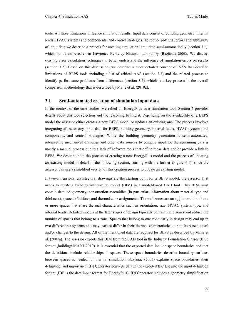
Chapter 4: Simulation AAS Tobias Maile
99
tools. All three limitations influence simulation results. Input data consist of building geometry, internal
loads, HVAC systems and components, and control strategies. To reduce potential errors and ambiguity
of input data we describe a process for creating simulation input data semi-automatically (section 3.1),
which builds on research at Lawrence Berkeley National Laboratory (Bazjanac 2008). We discuss
existing error calculation techniques to better understand the influence of simulation errors on results
(section 3.2). Based on this discussion, we describe a more detailed concept of AAS that describe
limitations of BEPS tools including a list of critical AAS (section 3.3) and the related process to
identify performance problems from differences (section 3.4), which is a key process in the overall
comparison methodology that is described by Maile et al. (2010a).
3.1 Semi-automated creation of simulation input data In the context of the case studies, we relied on EnergyPlus as a simulation tool. Section 4 provides
details about this tool selection and the reasoning behind it. Depending on the availability of a BEPS
model the assessor either creates a new BEPS model or updates an existing one. The process involves
integrating all necessary input data for BEPS, building geometry, internal loads, HVAC systems and
components, and control strategies. While the building geometry generation is semi-automated,
interpreting mechanical drawings and other data sources to compile input for the remaining data is
mostly a manual process due to a lack of software tools that define those data and/or provide a link to
BEPS. We describe both the process of creating a new EnergyPlus model and the process of updating
an existing model in detail in the following section, starting with the former (Figure 4-1), since the
assessor can use a simplified version of this creation process to update an existing model.
If two-dimensional architectural drawings are the starting point for a BEPS model, the assessor first
needs to create a building information model (BIM) in a model-based CAD tool. This BIM must
contain detailed geometry, construction assemblies (in particular, information about material type and
thickness), space definitions, and thermal zone assignments. Thermal zones are an agglomeration of one
or more spaces that share thermal characteristics such as orientation, size, HVAC system type, and
internal loads. Detailed models at the later stages of design typically contain more zones and reduce the
number of spaces that belong to a zone. Spaces that belong to one zone early in design may end up in
two different air systems and may start to differ in their thermal characteristics due to increased detail
and/or changes to the design. All of the mentioned data are required for BEPS as described by Maile et
al. (2007a). The assessor exports this BIM from the CAD tool in the Industry Foundation Classes (IFC)
format (buildingSMART 2010). It is essential that the exported data include space boundaries and that
the definitions include relationships to spaces. These space boundaries describe boundary surfaces
between spaces as needed for thermal simulation. Bazjanac (2005) explains space boundaries, their
definition, and importance. IDFGenerator converts data in the exported IFC file into the input definition
format (IDF is the data input format for EnergyPlus). IDFGenerator includes a geometry simplification

Chapter 4: Simulation AAS Tobias Maile
100
tool (GST) and uses predefined and embedded data transformation rules. Bazjanac (2008) discusses
these data transformation rules in detail. The resulting IDF file contains all relevant information and
data about the building geometry (including definitions of all materials and their thermal properties).
This IDF file also contains simulation run control parameters, such as convergence tolerances and the
simulation time period. GST/IDFGenerator also supports creation of partial IDF models (by spaces and
floors), which is helpful in encapsulating parts of the building during the comparison process.
Figure 4-1: Creation of an EnergyPlus model
The assessor needs to define HVAC systems and components manually in IDF format and add them to
a separate IDF file. Mechanical drawings form the basis for necessary data regarding HVAC system
topologies and HVAC component parameters. The assessor also gathers missing component data
(necessary for EnergyPlus objects) from manufacturer product specifications or field surveys. This task
is currently tedious, due to the lack of a comprehensive graphical user interface for EnergyPlus. Future
developments of EnergyPlus interfaces and data exchange capabilities with HVAC design applications
will help to simplify these tasks (e.g., LBNL 2010). Another important type of import data are the
control strategies of HVAC systems in the EnergyPlus model. The assessor can refer to mechanical
drawings and/or documents that describe the sequence of operations for these control strategies. It is
important to distinguish between original information (as established during design) and updated
information (as determined during field surveys). This differentiation is important, because we want to
establish a comparison between the original design BEPS model and actual operation as well as learn
about specific changes between final design and actual operation. The reasons and more importantly the
implications of these changes may not be known and may need further investigation within the
methodology to determine the implications. Finally, the assessor needs to update a weather file to
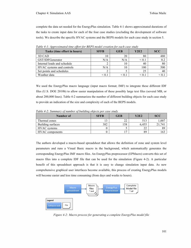
Chapter 4: Simulation AAS Tobias Maile
101
complete the data set needed for the EnergyPlus simulation. Table 4-1 shows approximated durations of
the tasks to create input data for each of the four case studies (excluding the development of software
tools). We describe the specific HVAC systems and the BEPS models for each case study in section 5.
Table 4-1: Approximated time effort for BEPS model creation for each case study Tasks (time effort in hours) SFFB GEB Y2E2 SCC
3D CAD 10 20 80 480 GST/IDFGenerator N/A N/A < 0.1 0.2 Internal loads and schedule 2 10 40 80 HVAC systems and controls N/A 10 100 500 Set points and schedules 2 5 25 40 Weather data < 0.1 < 0.1 < 0.1 < 0.1
We used the EnergyPlus macro language (input macro format; IMF) to integrate these different IDF
files (U.S. DOE 2010b) to allow easier manipulation of these possibly large text files (several MB, or
about 200,000 lines). Table 4-2 summarizes the number of different building objects for each case study
to provide an indication of the size and complexity of each of the BEPS models.
Table 4-2: Summary of number of building objects per case study Number of SFFB GEB Y2E2 SCC
Thermal zones 13 22 513 1,007 Building surfaces 382 158 6,455 21,741 HVAC systems 0 5 22 89 HVAC components 0 17 89 163
The authors developed a macro-based spreadsheet that allows the definition of zone and system level
parameters and runs a Visual Basic macro in the background, which automatically generates the
corresponding EnergyPlus IMF macro files. An EnergyPlus preprocessor (EPMacro) converts this set of
macro files into a complete IDF file that can be used for the simulation (Figure 4-2). A particular
benefit of this spreadsheet approach is that it is easy to change simulation input data. As new
comprehensive graphical user interfaces become available, this process of creating EnergyPlus models
will become easier and less time consuming (from days and weeks to hours).
Figure 4-2: Macro process for generating a complete EnergyPlus model file
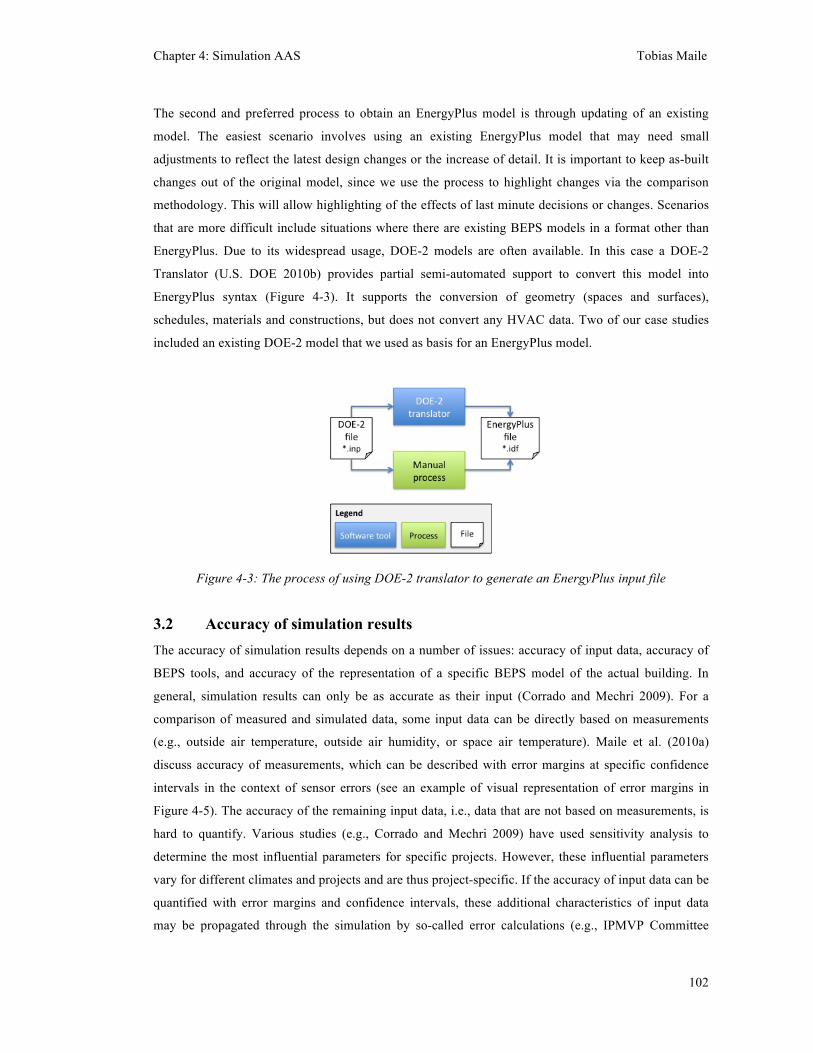
Chapter 4: Simulation AAS Tobias Maile
102
The second and preferred process to obtain an EnergyPlus model is through updating of an existing
model. The easiest scenario involves using an existing EnergyPlus model that may need small
adjustments to reflect the latest design changes or the increase of detail. It is important to keep as-built
changes out of the original model, since we use the process to highlight changes via the comparison
methodology. This will allow highlighting of the effects of last minute decisions or changes. Scenarios
that are more difficult include situations where there are existing BEPS models in a format other than
EnergyPlus. Due to its widespread usage, DOE-2 models are often available. In this case a DOE-2
Translator (U.S. DOE 2010b) provides partial semi-automated support to convert this model into
EnergyPlus syntax (Figure 4-3). It supports the conversion of geometry (spaces and surfaces),
schedules, materials and constructions, but does not convert any HVAC data. Two of our case studies
included an existing DOE-2 model that we used as basis for an EnergyPlus model.
Figure 4-3: The process of using DOE-2 translator to generate an EnergyPlus input file
3.2 Accuracy of simulation results The accuracy of simulation results depends on a number of issues: accuracy of input data, accuracy of
BEPS tools, and accuracy of the representation of a specific BEPS model of the actual building. In
general, simulation results can only be as accurate as their input (Corrado and Mechri 2009). For a
comparison of measured and simulated data, some input data can be directly based on measurements
(e.g., outside air temperature, outside air humidity, or space air temperature). Maile et al. (2010a)
discuss accuracy of measurements, which can be described with error margins at specific confidence
intervals in the context of sensor errors (see an example of visual representation of error margins in
Figure 4-5). The accuracy of the remaining input data, i.e., data that are not based on measurements, is
hard to quantify. Various studies (e.g., Corrado and Mechri 2009) have used sensitivity analysis to
determine the most influential parameters for specific projects. However, these influential parameters
vary for different climates and projects and are thus project-specific. If the accuracy of input data can be
quantified with error margins and confidence intervals, these additional characteristics of input data
may be propagated through the simulation by so-called error calculations (e.g., IPMVP Committee
Chapter 4: Simulation AAS Tobias Maile
103
2002; De Wit and Augenbroe 2002). However, error calculations do not consider the accuracy of the
equations embedded in BEPS tools or the appropriate use of the tool. These error calculations are
typically done for simulations that are based on a couple of equations. Since it is practically impossible
to quantify all sources of error, we describe the limitations of BEPS tools with AAS to enable an
assessment of simulation results compared to measurements. This approach is described in the
following subsection.
3.3 Identification of simulation assumptions, approximations, and
simplifications AAS are present in every simulation, since a simulation is always a reduction of a real life physical
process. For example, most simulation tools approximate the heat transfer calculation by using a spatial
1-dimensional approach instead of the real 3-dimensional. Approximations, assumptions, and
simplifications are defined as follows:
• Approximation: A mathematical quantity that is close in value to but not the same as a desired
quantity (Approximation 2010)
• Assumption: Something that one accepts as true without question or proof (Assumption 2010)
• Simplification: The process of making something less complicated and therefore easier to do
or understand (Simplification 2010)
Based on these definitions, we can differentiate among the AAS of BEPS models, those of input data,
and those related to the use of simulation concepts. AAS of BEPS models are embedded in the
simulation model, whereas AAS of input data describe how specific input data are derived. AAS related
to the use of simulation concepts reflect how users define and apply a specific aspect of the simulation.
These AAS, if contained in the model or input data, are usually not well documented and depend on
arbitrary decisions of users (Bazjanac 2008). Documenting these AAS is the basis for using them within
the EPCM and provides important details about the basis of the simulation model. Based on the three
definitions of AAS and their three different contexts (input data, model, and use), we have defined nine
categories of AAS for EPCM. We developed a list of critical simulation AAS based on existing
literature and applied it to each of the case studies. This list uses the nine categories of AAS as follows.
For each item, the relevant case studies (if any) and reference information are given in parentheses. We
provide details about the BEPS models and their limitations and AAS for each case study in section 5.
Input data approximations:
1. Diffuse solar radiation is approximated with a solar model and total radiation measurements
(SFFB, GEB, Duffie and Beckman 1980)
2. Wind direction and speed are approximated based on façade pressure difference (SFFB)

Chapter 4: Simulation AAS Tobias Maile
104
Model approximations:
3. View factor approximation of surfaces is appropriate (SFFB, GEB, Y2E2, SCC; U.S. DOE
2010c)
Usage approximations:
4. Internal loads are approximated on the space level from floor level measurements (Y2E2)
5. The district chilled/hot water object can approximate the performance of other not supported
supply (Y2E2, GEB)
6. Connected multi-temperature water loops are approximated with standalone water loops
(Y2E2)
7. (Sinus-) curved surfaced are approximated with rectangular planar surfaces (SFFB)
Input data assumptions:
8. Zone infiltration is typical (GEB, Y2E2, SCC; Gowri et al. 2009)
9. Wall constructions are built based on design specifications (SFFB, GEB, Y2E2, SCC)
10. Manufacturer data of HVAC components reflect actual performance (GEB, Y2E2, SCC)
11. Heat gains from lights are assumed to appear as zone loads (SFFB, GEB, Y2E2, SCC; U.S.
DOE 2010d)
Model assumptions:
12. Buildings do not have curved walls, columns, beams, and non-rectangular walls (GEB, SFFB,
Y2E2, SCC)
13. Relationship between valve position and air flow is proportional (Y2E2)
14. Idealized models assume that the thermal box can reduce the flow rate to the design minimum
value (Y2E2)
15. Windows and solar collectors are always clean (Y2E2; U.S. DOE 2010c)
16. Component performance is constant (no degradation; SFFB, GEB, Y2E2, SCC)
17. Façade Cp pressure values represent actual conditions (SFFB, Y2E2; Ferson et al. 2008)
18. Ducts are perfectly insulated (GEB, Y2E2, SCC; Klote 1988)
19. Ducts have no air leakage (GEB, Y2E2, SCC)
20. No air stream reheating is provided by the circulation fans or by the ducts (Y2E2)
Usage assumptions:
21. Heat transfer between floors is ignored (partial model; SFFB)
22. Internal loads represent actual building usage (SFFB, GEB, Y2E2, SCC; Morrissey 2006)
23. Thermal subzones are somewhat arbitrary (SFFB; Pati et al. 2006)

Chapter 4: Simulation AAS Tobias Maile
105
24. Zone temperature set point for a set of zones is identical (Y2E2)
25. Zone infiltration loads are negligible or considered part of the ventilation loads (SFFB; Suwon
2007)
26. Zone solar and transmission loads affect the perimeter zones only (Y2E2, SCC; )
27. A single air flow return path is representative of the actual splitter return path (Y2E2)
28. Two level branching represents three level branching (Y2E2)
29. Splitting of thermal zones because of zone equipment limitations is acceptable (Y2E2)
30. Boundary walls of partial models are adiabatic (SFFB, Y2E2)
31. Control strategy is based on temperature control only (Y2E2)
32. A specific component performance (e.g., cooling tower, hot steam supply and related heat
exchanger) performance can be neglected (GEB, Y2E2)
Input data simplifications:
33. HVAC model configuration is simplified (GEB, Y2E2, SCC)
34. Surrounding shading objects (e.g., trees) are simplified (SFFB, Y2E2; U.S. DOE 2010c)
Model simplifications:
35. Control response time is instantaneous (SFFB, GEB, Y2E2, SCC)
36. Airflow model assumes bulk air flow at the zone/space level (SFFB)
37. Zone is well-mixed (SFFB, GEB, Y2E2, SCC; Li 2009, Energy Design Resources 2005)
38. Pressure drop is neglected (Y2E2, GEB, SCC; U.S. DOE 2010d)
Usage simplifications:
39. The BEPS simulation model uses perimeter/core zone modeling compared to zone type
modeling (GSA 2009)
40. Internal loads are on a regular schedule (SFFB, GEB, Y2E2, SCC)
41. Splitting of HVAC systems does not have major influences on the results (SCC)
42. Dedicated pump configuration is simplified with a headered (parallel) pump configuration
(Y2E2, SCC)
This list of simulation AAS is the first formal compilation of AAS for BEPS based on literature and
four case studies. The formalization of these AAS is a first step towards understanding the implications
and effects of the AAS. Thus, we compiled a table in Appendix C that adds anticipated effects to each
AAS. These anticipated effects support the assessor in evaluating simulation results. The second step is
to minimize these AAS (and thus limitations) in the use, development, and input of BEPS models. We
discuss further research areas based on this AAS list in section 8.4.
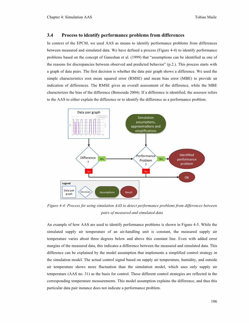
Chapter 4: Simulation AAS Tobias Maile
106
3.4 Process to identify performance problems from differences In context of the EPCM, we used AAS as means to identify performance problems from differences
between measured and simulated data. We have defined a process (Figure 4-4) to identify performance
problems based on the concept of Ganeshan et al. (1999) that “assumptions can be identified as one of
the reasons for discrepancies between observed and predicted behavior” (p.2.). This process starts with
a graph of data pairs. The first decision is whether the data pair graph shows a difference. We used the
simple characteristics root mean squared error (RMSE) and mean bias error (MBE) to provide an
indication of differences. The RMSE gives an overall assessment of the difference, while the MBE
characterizes the bias of the difference (Bensouda 2004). If a difference is identified, the assessor refers
to the AAS to either explain the difference or to identify the difference as a performance problem.
Figure 4-4: Process for using simulation AAS to detect performance problems from differences between
pairs of measured and simulated data
An example of how AAS are used to identify performance problems is shown in Figure 4-5. While the
simulated supply air temperature of an air-handling unit is constant, the measured supply air
temperature varies about three degrees below and above this constant line. Even with added error
margins of the measured data, this indicates a difference between the measured and simulated data. This
difference can be explained by the model assumption that implements a simplified control strategy in
the simulation model. The actual control signal based on supply air temperature, humidity, and outside
air temperature shows more fluctuation than the simulation model, which uses only supply air
temperature (AAS no. 31) as the basis for control. These different control strategies are reflected in the
corresponding temperature measurements. This model assumption explains the difference, and thus this
particular data pair instance does not indicate a performance problem.
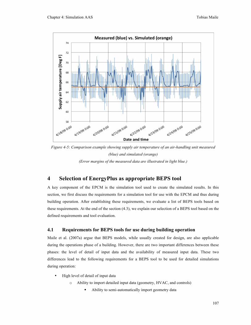
Chapter 4: Simulation AAS Tobias Maile
107
Figure 4-5: Comparison example showing supply air temperature of an air-handling unit measured
(blue) and simulated (orange)
(Error margins of the measured data are illustrated in light blue.)
4 Selection of EnergyPlus as appropriate BEPS tool A key component of the EPCM is the simulation tool used to create the simulated results. In this
section, we first discuss the requirements for a simulation tool for use with the EPCM and thus during
building operation. After establishing these requirements, we evaluate a list of BEPS tools based on
these requirements. At the end of the section (4.3), we explain our selection of a BEPS tool based on the
defined requirements and tool evaluation.
4.1 Requirements for BEPS tools for use during building operation Maile et al. (2007a) argue that BEPS models, while usually created for design, are also applicable
during the operations phase of a building. However, there are two important differences between these
phases: the level of detail of input data and the availability of measured input data. These two
differences lead to the following requirements for a BEPS tool to be used for detailed simulations
during operation:
• High level of detail of input data
o Ability to import detailed input data (geometry, HVAC, and controls)
Ability to semi-automatically import geometry data
Chapter 4: Simulation AAS Tobias Maile
108
Ability to model detailed and complex HVAC configurations
Ability to model detailed control strategies
o Ability to adjust HVAC component equations
o Ability to simulate at a small time scale
o Ability to model complex geometry
o Ability to consider feedback from HVAC systems
• Input of measured data
o Ability to automatically import detailed measured input data
o Ability to “override” simulated data with measured data (to support partial models)
The level of detail of a BEPS model increases with design stages, possibly resulting in a very detailed
model at the final design stages. One reason for the increase of detail is that more information about the
building is generated during design and finalized during construction. For example, during conceptual
design the simulation expert may aggregate most of the office spaces into one combined office zone
(depending on orientation and other influences) that is served by the same HVAC system, uses the same
zone level components, and has similar internal loads. During later stages of the design process,
similarities of these aggregated zones may change due to the increased level of detail and design
changes; thus spaces that were similar in the early design stages and contained in one zone may be
different and aggregated in different zones. In particular, at the operations stage, ducting and
relationships among HVAC components are known (assuming they are documented accurately) and this
enables the modeling of the actual building in greater detail. For a comparison with actual data, it is
important to represent the building with the same level of detail, to enable a one-to-one matching
between measured and simulated data.
This increased level of detail compared to the typical detail of BEPS models at early design stages
requires the ability of the BEPS tool to capture such a high level of detail. This high level of detail is
required for all types of input data: geometry, HVAC, and controls. To achieve this high level of detail,
data exchange between CAD tools and BEPS tools becomes an important issue. While the effort of the
initial creation of the energy model depends greatly on the amount of data one needs to manually
import, the manual import of data increases this effort even more dramatically if various versions and
modifications of a model are needed. Since BIMs contain those data, we have defined import of BIM-
based geometry as a requirement. Bazjanac (2001) states that a BIM-‐based geometry input can
reduce the modeling effort for geometry by 70-‐80%.
The requirement for a high level of detail also applies for HVAC systems and system topologies that are
supported by a BEPS tool. BEPS tools that are more flexible can support more real-life buildings than
tools that provide a rather stringent system topology. A tool should cover all common system types,
including air, hot and cold water, steam, and electricity systems. BEPS tools with discrete HVAC
Chapter 4: Simulation AAS Tobias Maile
109
components are more flexible in their HVAC topologies than BESP tools that have predefined HVAC
systems.
In addition, the need for detail poses requirements for the representation of controls in BEPS tools.
Typically, three levels of control strategies are available in BEPS tools: simplified, equation-based, and
realistic (with time delays). Simplified control strategies are based on a predefined set of strategies,
where the user can specify set points and reference nodes, but cannot change underlying equations.
Equation-based control strategies allow the user to define these equations, providing a high level of
flexibility. Realistic control modeling is usually possible with the use of separate tools to design control
strategies (such as Matlab/Simulink, etc.) that also consider time delay of controls and smoothing of
control signals. To use those external design control tools, a link between BEPS tools and design
control tools is necessary.
Furthermore, the simulation tool should include a mechanism to simulate all HVAC components and
strategies employed for a building, or at least provide a mechanism to account for components that
cannot be modeled due to missing functionality. Ideally a BEPS tool allows the user to adjust existing
component equations to allow for flexibility or at least provides component models with different levels
of detail. This is particularly important to enable the evaluation of new and innovative HVAC
components or configurations.
Besides the level of detail of the model structure and data, the time resolution is also important. Maile et
al. (2010a) argue for a one-minute resolution for measurements. Thus, we require the same resolution
for BEPS tools.
Simulating energy performance at this high level of detail also requires two additional functionalities:
representation of complex geometry and feedback of underperforming HVAC systems to space
conditions. With the increasing complexity of the geometry of buildings, the simulation tool needs an
appropriate geometric model. We formulated this requirement with the need for multisided planar
polygons. More complex geometry, such as curved surfaces, can be approximated with the use of
multisided polygons.
The feedback from the HVAC system response to the space or zone must also be provided at the
required level of detail. Without this feedback, the BEPS tool does not account for undersized systems,
and the resulting space temperatures (and other space parameters) do not show the effects of such. Since
an undersized HVAC system will have an effect on the space conditions in the actual building, the
BEPS tool needs to consider this effect as well. Integrating system and zone simulation allows
accounting for these system deficiencies (Hensen and Clarke 2000; Trcka and Hensen 2009). Thus we
require an integrated simulation of HVAC systems and spaces, including the necessary feedback from
systems to zones.
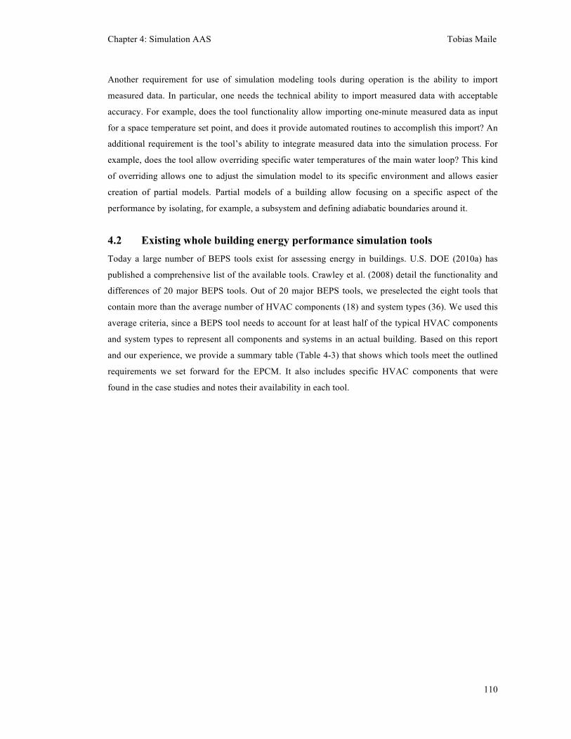
Chapter 4: Simulation AAS Tobias Maile
110
Another requirement for use of simulation modeling tools during operation is the ability to import
measured data. In particular, one needs the technical ability to import measured data with acceptable
accuracy. For example, does the tool functionality allow importing one-minute measured data as input
for a space temperature set point, and does it provide automated routines to accomplish this import? An
additional requirement is the tool’s ability to integrate measured data into the simulation process. For
example, does the tool allow overriding specific water temperatures of the main water loop? This kind
of overriding allows one to adjust the simulation model to its specific environment and allows easier
creation of partial models. Partial models of a building allow focusing on a specific aspect of the
performance by isolating, for example, a subsystem and defining adiabatic boundaries around it.
4.2 Existing whole building energy performance simulation tools Today a large number of BEPS tools exist for assessing energy in buildings. U.S. DOE (2010a) has
published a comprehensive list of the available tools. Crawley et al. (2008) detail the functionality and
differences of 20 major BEPS tools. Out of 20 major BEPS tools, we preselected the eight tools that
contain more than the average number of HVAC components (18) and system types (36). We used this
average criteria, since a BEPS tool needs to account for at least half of the typical HVAC components
and system types to represent all components and systems in an actual building. Based on this report
and our experience, we provide a summary table (Table 4-3) that shows which tools meet the outlined
requirements we set forward for the EPCM. It also includes specific HVAC components that were
found in the case studies and notes their availability in each tool.
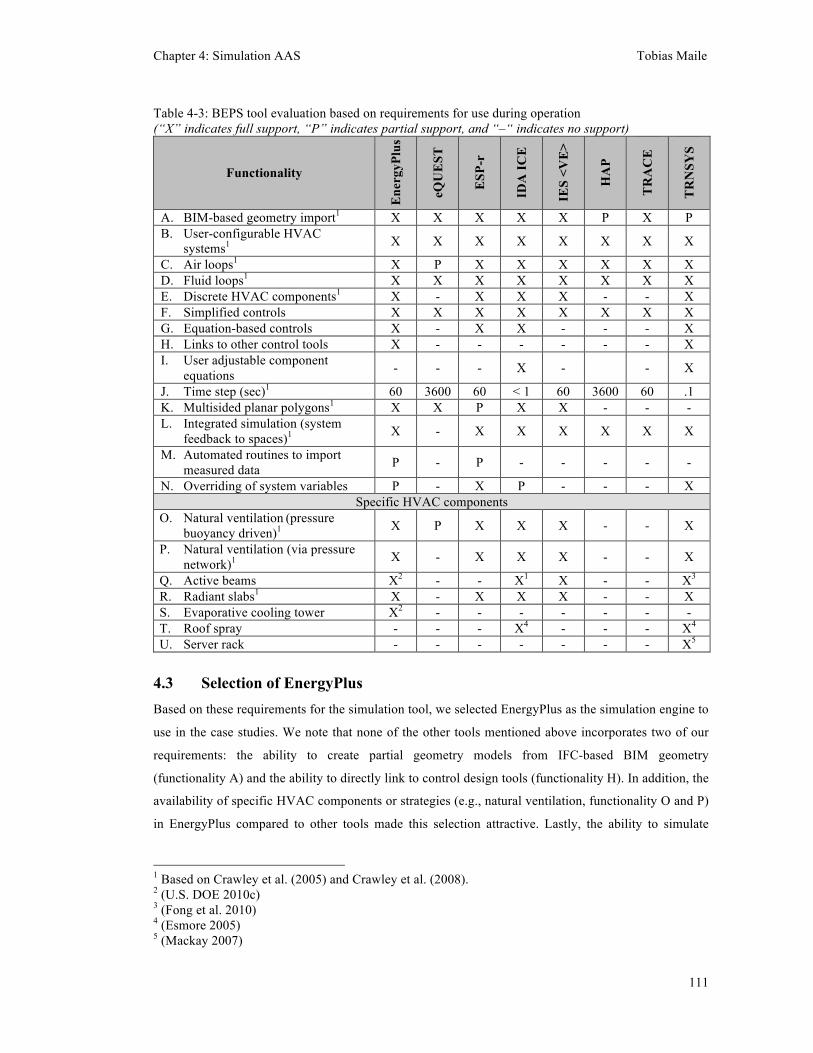
Chapter 4: Simulation AAS Tobias Maile
111
Table 4-3: BEPS tool evaluation based on requirements for use during operation (“X” indicates full support, “P” indicates partial support, and “–“ indicates no support)
Functionality
Ene
rgyP
lus
eQU
EST
ESP
-r
IDA
ICE
IES
<VE
>
HA
P
TR
AC
E
TR
NSY
S
A. BIM-based geometry import1 X X X X X P X P B. User-configurable HVAC
systems1 X X X X X X X X
C. Air loops1 X P X X X X X X D. Fluid loops1 X X X X X X X X E. Discrete HVAC components1 X - X X X - - X F. Simplified controls X X X X X X X X G. Equation-based controls X - X X - - - X H. Links to other control tools X - - - - - - X I. User adjustable component
equations - - - X - - X
J. Time step (sec)1 60 3600 60 < 1 60 3600 60 .1 K. Multisided planar polygons1 X X P X X - - - L. Integrated simulation (system
feedback to spaces)1 X - X X X X X X
M. Automated routines to import measured data P - P - - - - -
N. Overriding of system variables P - X P - - - X Specific HVAC components
O. Natural ventilation (pressure buoyancy driven)1 X P X X X - - X
P. Natural ventilation (via pressure network)1 X - X X X - - X
Q. Active beams X2 - - X1 X - - X3 R. Radiant slabs1 X - X X X - - X S. Evaporative cooling tower X2 - - - - - - - T. Roof spray - - - X4 - - - X4 U. Server rack - - - - - - - X5
4.3 Selection of EnergyPlus Based on these requirements for the simulation tool, we selected EnergyPlus as the simulation engine to
use in the case studies. We note that none of the other tools mentioned above incorporates two of our
requirements: the ability to create partial geometry models from IFC-based BIM geometry
(functionality A) and the ability to directly link to control design tools (functionality H). In addition, the
availability of specific HVAC components or strategies (e.g., natural ventilation, functionality O and P)
in EnergyPlus compared to other tools made this selection attractive. Lastly, the ability to simulate
1 Based on Crawley et al. (2005) and Crawley et al. (2008). 2 (U.S. DOE 2010c) 3 (Fong et al. 2010) 4 (Esmore 2005) 5 (Mackay 2007)
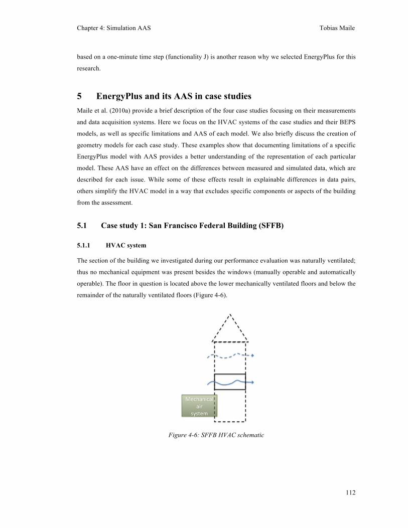
Chapter 4: Simulation AAS Tobias Maile
112
based on a one-minute time step (functionality J) is another reason why we selected EnergyPlus for this
research.
5 EnergyPlus and its AAS in case studies Maile et al. (2010a) provide a brief description of the four case studies focusing on their measurements
and data acquisition systems. Here we focus on the HVAC systems of the case studies and their BEPS
models, as well as specific limitations and AAS of each model. We also briefly discuss the creation of
geometry models for each case study. These examples show that documenting limitations of a specific
EnergyPlus model with AAS provides a better understanding of the representation of each particular
model. These AAS have an effect on the differences between measured and simulated data, which are
described for each issue. While some of these effects result in explainable differences in data pairs,
others simplify the HVAC model in a way that excludes specific components or aspects of the building
from the assessment.
5.1 Case study 1: San Francisco Federal Building (SFFB)
5.1.1 HVAC system
The section of the building we investigated during our performance evaluation was naturally ventilated;
thus no mechanical equipment was present besides the windows (manually operable and automatically
operable). The floor in question is located above the lower mechanically ventilated floors and below the
remainder of the naturally ventilated floors (Figure 4-6).
Figure 4-6: SFFB HVAC schematic

Chapter 4: Simulation AAS Tobias Maile
113
5.1.2 Design BEPS model
An existing design EnergyPlus model (Carrilho da Graca et al. 2004) was used as the basis for our
EnergyPlus model for this assessment. We adjusted the building geometry to incorporate more detail; in
particular the sinus wave shaped ceiling was approximated with higher detail than in the existing model.
EnergyPlus provides an advanced AirFlowNetwork module (based on COMIS (EETD 2003)), which
uses nodal airflow calculations. This AirFlowNetwork required pressure coefficients (so-called Cp-
Values), which describe how wind reacts to the façade. Wind tunnel test data collected during design
provided these values (Rauscher et al. 2002).
5.1.3 Usage approximations, assumptions, and simplifications
The vertical boundary to the non-modeled part of the 6th floor was defined as adiabatic, assuming no
major difference between the two floor elements in terms of temperature (AAS no. 21). The floor
surface boundaries on top and bottom were interlinked in EnergyPlus. For most parts of the model, this
adiabatic assumption seems reasonable, since most spaces are full height, and thus the temperature
difference between the two spaces (which in fact are the same) is zero. While it is relative unlikely that
major temperature differences exist between floors that are naturally ventilated, it is possible that an
unknown temperature difference could exist between the modeled floor and the lower floor (5th floor),
which is mechanically air-conditioned.
The main approximation within this model is the partial geometry of the building that assumes that
boundary walls are adiabatic (AAS no. 30). The selected section is on the 6th floor of the building. The
effect of airflow in neighboring sections of the 6th floor is unknown and may vary depending on wind
direction and speed. These uncertainties about the influences of processes that are close to the
instrumented section of the building could not be quantified, since there were no measurements to
detected them.
A simplification embedded in this EnergyPlus model is the representation of the sinus waved ceiling.
Since EnergyPlus does not allow for curved surfaces, this ceiling was simplified using rectangular
planar surfaces (AAS no. 7).
5.2 Case study 2: Global Ecology Building (GEB)
5.2.1 HVAC system
The HVAC system at GEB contains several innovative features (Figure 4-7). A so-called evaporative
cooling tower in the lobby entrance area aims to cool the lobby in the summer through natural
convection based on the use of sprayed water evaporating in this tower. The lobby also features large
glass doors that can be opened during the summer to provide a transitional space between outside and
inside. In the winter, a radiant slab heats the lobby. The first floor is mechanically cooled and heated by
Chapter 4: Simulation AAS Tobias Maile
114
the main air handler, with an additional fan coil unit cooling at the zone level. This main air handler has
an economizer and is single ducted. In addition, fume hoods are installed where necessary for lab
exhaust. The second floor is fully naturally ventilated, except for the mechanically cooled server room.
The hot water system is a typical system with two boilers, whereas the chilled water system uses a
chiller and a night sky spray connected to a chilled water tank as source of cooling energy. The night
sky spray evaporates water into the air on the roof during sufficiently cold nights to cool the water
naturally.
Figure 4-7: GEB HVAC schematic
5.2.2 Design BEPS model
A DOE-2 model was created by the designer during design of the building. We created the EnergyPlus
model based on this DOE-2 model with the help of the DOE-2 Translator (see section 3.1). This
translator automatically converts parts of a DOE-2 model into EnergyPlus input format.
5.2.3 Usage approximations, assumptions, and simplifications
The innovative HVAC system at GEB was difficult to model in EnergyPlus at the time of the project,
because multiple components were not available as EnergyPlus objects, including the evaporative
cooling tower (which was added in a later version of EnergyPlus) and the roof spray system. These
missing components needed to be modeled with workarounds to include them into the model. Our
model simplified the roof spray system with a district chilled water object (AAS no. 5; Figure 4-8) and
ignored the cooling tower in the lobby (AAS no. 32) due to the missing availability in EnergyPlus. The
district cooling simplification excluded the roof spray from the evaluation. Thus, problems with these
two components cannot be detected using the EPCM. To enable evaluation of the remainder of the
chilled water loop components, the measured supply water temperature was used as the supply water
temperature set point to recreate the conditions that the roof spray provides.
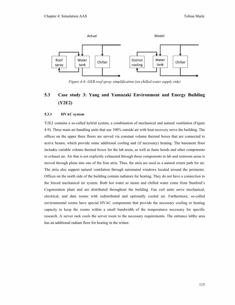
Chapter 4: Simulation AAS Tobias Maile
115
Figure 4-8: GEB roof spray simplification (on chilled water supply side)
5.3 Case study 3: Yang and Yamazaki Environment and Energy Building
(Y2E2)
5.3.1 HVAC system
Y2E2 contains a so-called hybrid system, a combination of mechanical and natural ventilation (Figure
4-9). Three main air-handling units that use 100% outside air with heat recovery serve the building. The
offices on the upper three floors are served via constant volume thermal boxes that are connected to
active beams, which provide some additional cooling and (if necessary) heating. The basement floor
includes variable volume thermal boxes for the lab areas, as well as fume hoods and other components
to exhaust air. Air that is not explicitly exhausted through those components in lab and restroom areas is
moved through plena into one of the four atria. Thus, the atria are used as a natural return path for air.
The atria also support natural ventilation through automated windows located around the perimeter.
Offices on the north side of the building contain radiators for heating. They do not have a connection to
the forced mechanical air system. Both hot water as steam and chilled water come from Stanford’s
Cogeneration plant and are distributed throughout the building. Fan coil units serve mechanical,
electrical, and data rooms with redistributed and optionally cooled air. Furthermore, so-called
environmental rooms have special HVAC components that provide the necessary cooling or heating
capacity to keep the rooms within a small bandwidth of the temperatures necessary for specific
research. A server rack cools the server room to the necessary requirements. The entrance lobby area
has an additional radiant floor for heating in the winter.
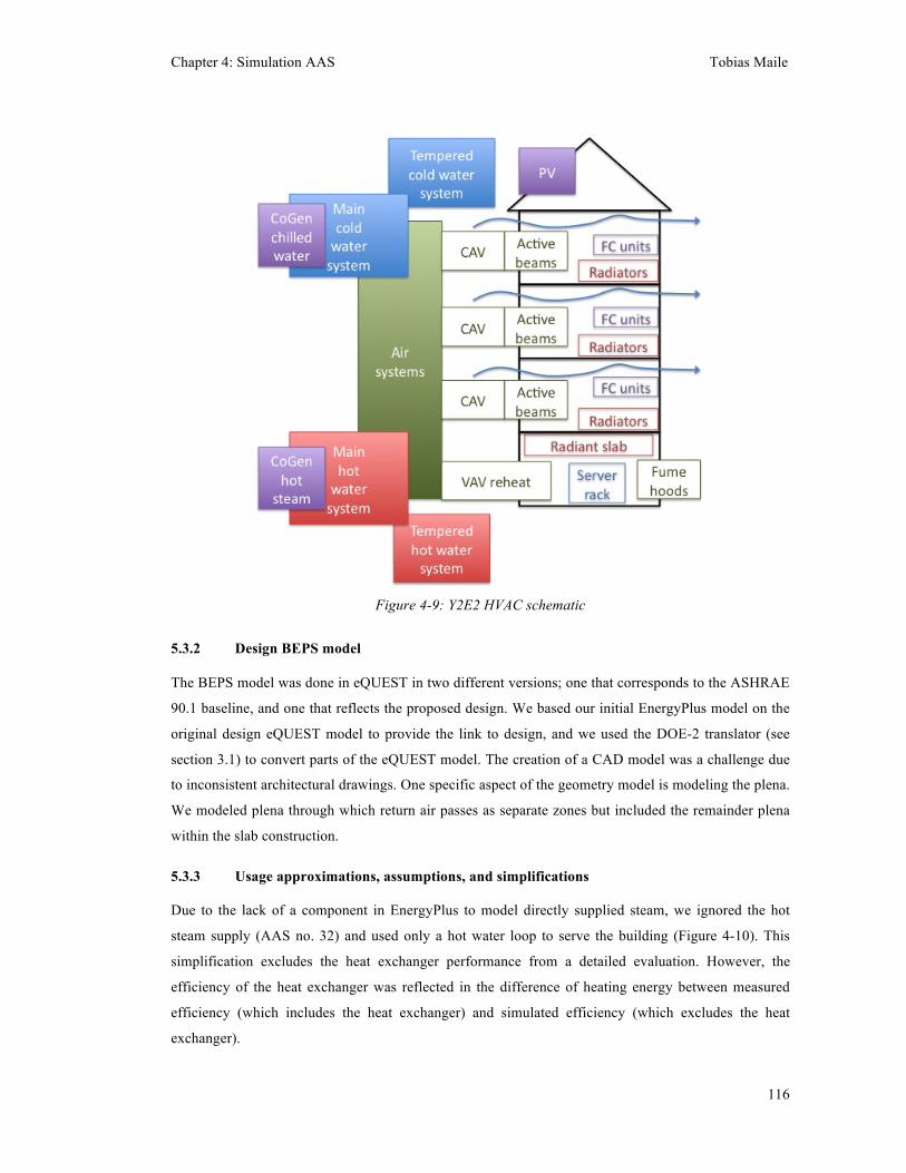
Chapter 4: Simulation AAS Tobias Maile
116
Figure 4-9: Y2E2 HVAC schematic
5.3.2 Design BEPS model
The BEPS model was done in eQUEST in two different versions; one that corresponds to the ASHRAE
90.1 baseline, and one that reflects the proposed design. We based our initial EnergyPlus model on the
original design eQUEST model to provide the link to design, and we used the DOE-2 translator (see
section 3.1) to convert parts of the eQUEST model. The creation of a CAD model was a challenge due
to inconsistent architectural drawings. One specific aspect of the geometry model is modeling the plena.
We modeled plena through which return air passes as separate zones but included the remainder plena
within the slab construction.
5.3.3 Usage approximations, assumptions, and simplifications
Due to the lack of a component in EnergyPlus to model directly supplied steam, we ignored the hot
steam supply (AAS no. 32) and used only a hot water loop to serve the building (Figure 4-10). This
simplification excludes the heat exchanger performance from a detailed evaluation. However, the
efficiency of the heat exchanger was reflected in the difference of heating energy between measured
efficiency (which includes the heat exchanger) and simulated efficiency (which excludes the heat
exchanger).
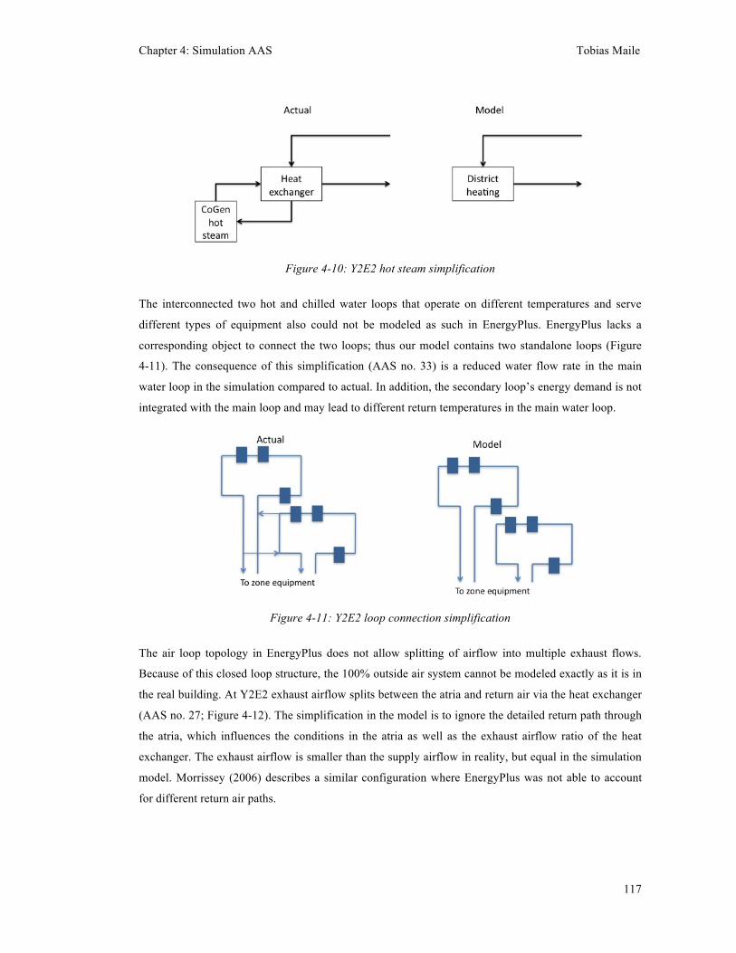
Chapter 4: Simulation AAS Tobias Maile
117
Figure 4-10: Y2E2 hot steam simplification
The interconnected two hot and chilled water loops that operate on different temperatures and serve
different types of equipment also could not be modeled as such in EnergyPlus. EnergyPlus lacks a
corresponding object to connect the two loops; thus our model contains two standalone loops (Figure
4-11). The consequence of this simplification (AAS no. 33) is a reduced water flow rate in the main
water loop in the simulation compared to actual. In addition, the secondary loop’s energy demand is not
integrated with the main loop and may lead to different return temperatures in the main water loop.
Figure 4-11: Y2E2 loop connection simplification
The air loop topology in EnergyPlus does not allow splitting of airflow into multiple exhaust flows.
Because of this closed loop structure, the 100% outside air system cannot be modeled exactly as it is in
the real building. At Y2E2 exhaust airflow splits between the atria and return air via the heat exchanger
(AAS no. 27; Figure 4-12). The simplification in the model is to ignore the detailed return path through
the atria, which influences the conditions in the atria as well as the exhaust airflow ratio of the heat
exchanger. The exhaust airflow is smaller than the supply airflow in reality, but equal in the simulation
model. Morrissey (2006) describes a similar configuration where EnergyPlus was not able to account
for different return air paths.
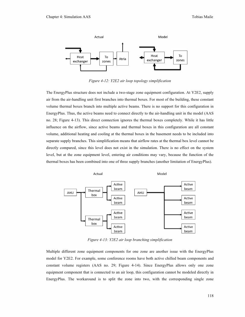
Chapter 4: Simulation AAS Tobias Maile
118
Figure 4-12: Y2E2 air loop topology simplification
The EnergyPlus structure does not include a two-stage zone equipment configuration. At Y2E2, supply
air from the air-handling unit first branches into thermal boxes. For most of the building, these constant
volume thermal boxes branch into multiple active beams. There is no support for this configuration in
EnergyPlus. Thus, the active beams need to connect directly to the air-handling unit in the model (AAS
no. 28; Figure 4-13). This direct connection ignores the thermal boxes completely. While it has little
influence on the airflow, since active beams and thermal boxes in this configuration are all constant
volume, additional heating and cooling at the thermal boxes in the basement needs to be included into
separate supply branches. This simplification means that airflow rates at the thermal box level cannot be
directly compared, since this level does not exist in the simulation. There is no effect on the system
level, but at the zone equipment level, entering air conditions may vary, because the function of the
thermal boxes has been combined into one of three supply branches (another limitation of EnergyPlus).
Figure 4-13: Y2E2 air loop branching simplification
Multiple different zone equipment components for one zone are another issue with the EnergyPlus
model for Y2E2. For example, some conference rooms have both active chilled beam components and
constant volume registers (AAS no. 29; Figure 4-14). Since EnergyPlus allows only one zone
equipment component that is connected to an air loop, this configuration cannot be modeled directly in
EnergyPlus. The workaround is to split the zone into two, with the corresponding single zone
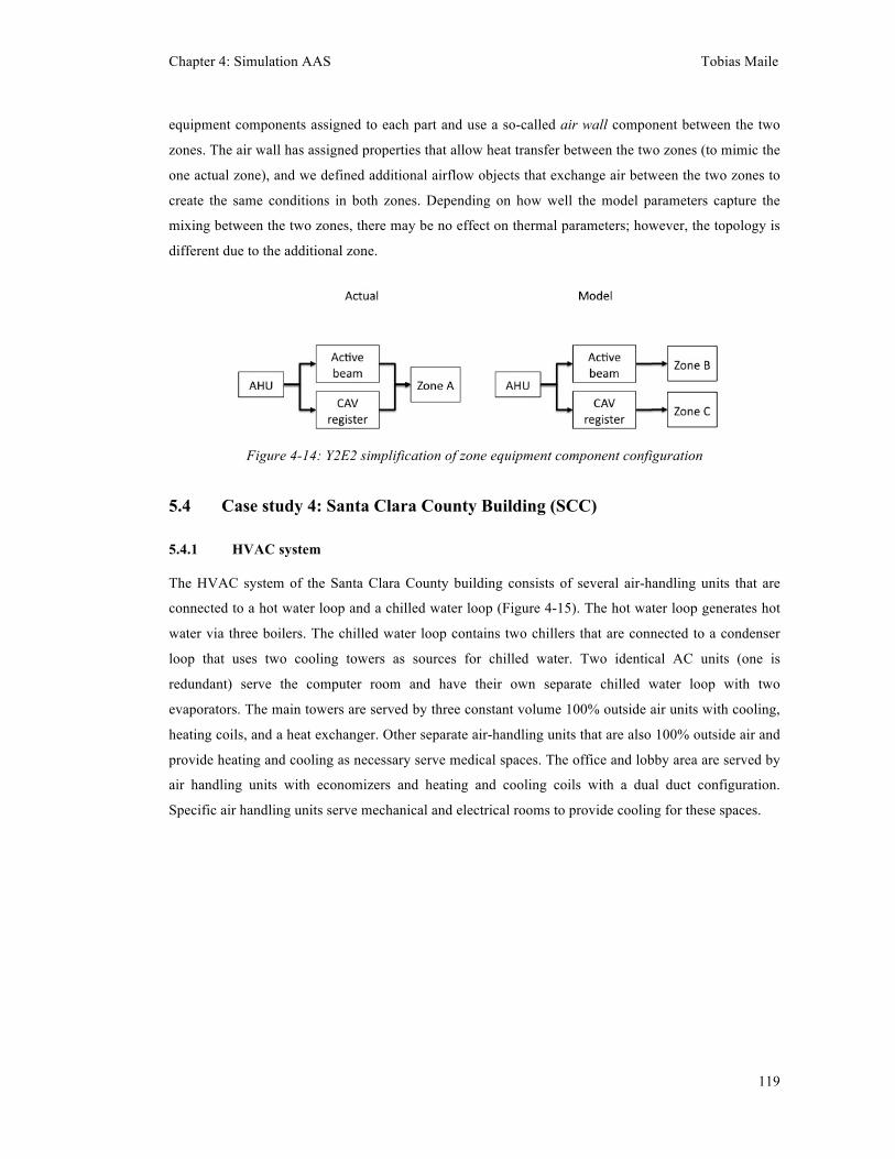
Chapter 4: Simulation AAS Tobias Maile
119
equipment components assigned to each part and use a so-called air wall component between the two
zones. The air wall has assigned properties that allow heat transfer between the two zones (to mimic the
one actual zone), and we defined additional airflow objects that exchange air between the two zones to
create the same conditions in both zones. Depending on how well the model parameters capture the
mixing between the two zones, there may be no effect on thermal parameters; however, the topology is
different due to the additional zone.
Figure 4-14: Y2E2 simplification of zone equipment component configuration
5.4 Case study 4: Santa Clara County Building (SCC)
5.4.1 HVAC system
The HVAC system of the Santa Clara County building consists of several air-handling units that are
connected to a hot water loop and a chilled water loop (Figure 4-15). The hot water loop generates hot
water via three boilers. The chilled water loop contains two chillers that are connected to a condenser
loop that uses two cooling towers as sources for chilled water. Two identical AC units (one is
redundant) serve the computer room and have their own separate chilled water loop with two
evaporators. The main towers are served by three constant volume 100% outside air units with cooling,
heating coils, and a heat exchanger. Other separate air-handling units that are also 100% outside air and
provide heating and cooling as necessary serve medical spaces. The office and lobby area are served by
air handling units with economizers and heating and cooling coils with a dual duct configuration.
Specific air handling units serve mechanical and electrical rooms to provide cooling for these spaces.
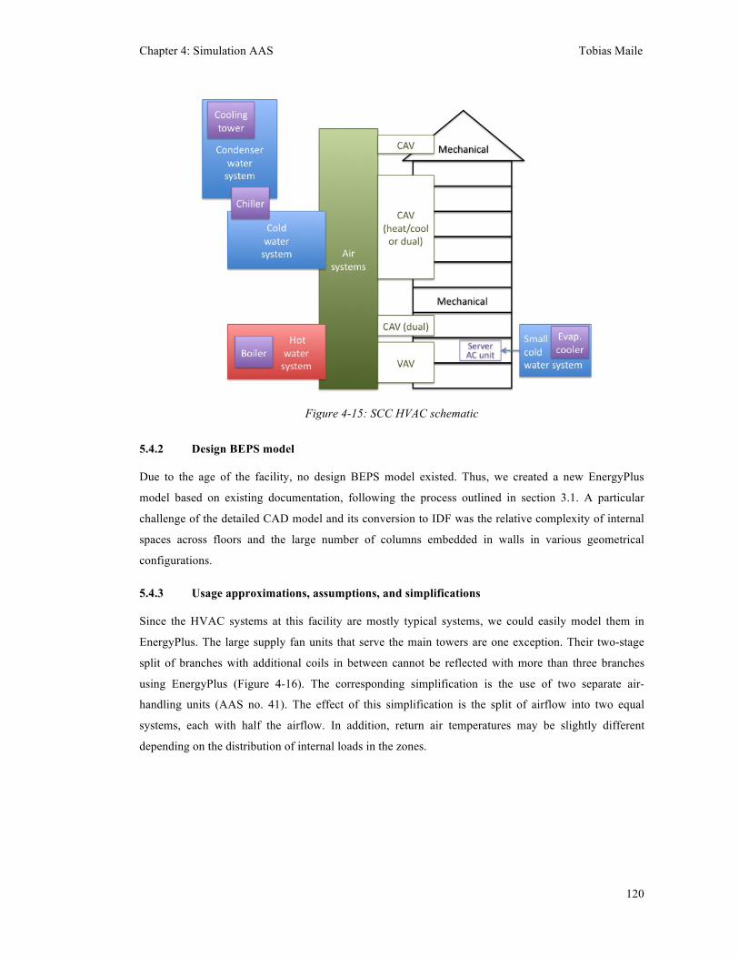
Chapter 4: Simulation AAS Tobias Maile
120
Figure 4-15: SCC HVAC schematic
5.4.2 Design BEPS model
Due to the age of the facility, no design BEPS model existed. Thus, we created a new EnergyPlus
model based on existing documentation, following the process outlined in section 3.1. A particular
challenge of the detailed CAD model and its conversion to IDF was the relative complexity of internal
spaces across floors and the large number of columns embedded in walls in various geometrical
configurations.
5.4.3 Usage approximations, assumptions, and simplifications
Since the HVAC systems at this facility are mostly typical systems, we could easily model them in
EnergyPlus. The large supply fan units that serve the main towers are one exception. Their two-stage
split of branches with additional coils in between cannot be reflected with more than three branches
using EnergyPlus (Figure 4-16). The corresponding simplification is the use of two separate air-
handling units (AAS no. 41). The effect of this simplification is the split of airflow into two equal
systems, each with half the airflow. In addition, return air temperatures may be slightly different
depending on the distribution of internal loads in the zones.
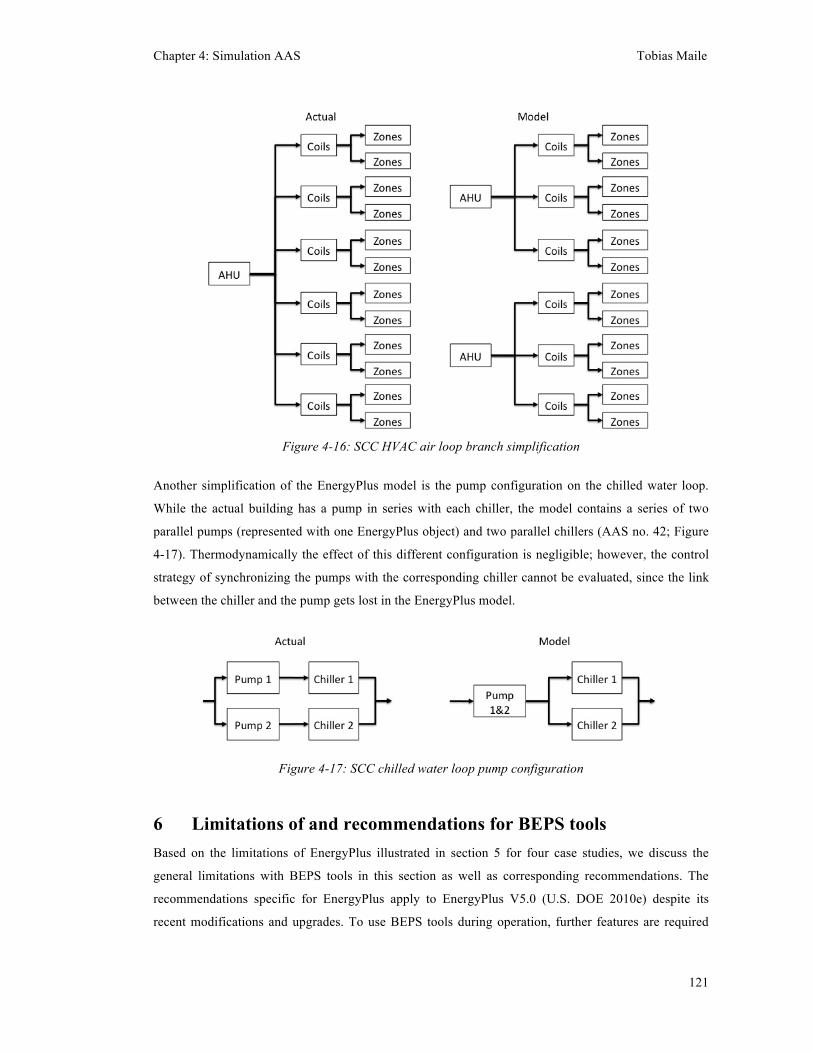
Chapter 4: Simulation AAS Tobias Maile
121
Figure 4-16: SCC HVAC air loop branch simplification
Another simplification of the EnergyPlus model is the pump configuration on the chilled water loop.
While the actual building has a pump in series with each chiller, the model contains a series of two
parallel pumps (represented with one EnergyPlus object) and two parallel chillers (AAS no. 42; Figure
4-17). Thermodynamically the effect of this different configuration is negligible; however, the control
strategy of synchronizing the pumps with the corresponding chiller cannot be evaluated, since the link
between the chiller and the pump gets lost in the EnergyPlus model.
Figure 4-17: SCC chilled water loop pump configuration
6 Limitations of and recommendations for BEPS tools Based on the limitations of EnergyPlus illustrated in section 5 for four case studies, we discuss the
general limitations with BEPS tools in this section as well as corresponding recommendations. The
recommendations specific for EnergyPlus apply to EnergyPlus V5.0 (U.S. DOE 2010e) despite its
recent modifications and upgrades. To use BEPS tools during operation, further features are required

Chapter 4: Simulation AAS Tobias Maile
122
(see 4.1), which have not been addressed in recent EnergyPlus or other BEPS tool developments. The
major conceptual limitations of BEPS tools are inadequate geometric representation (section 6.1),
inability to model innovative, unique, and unorthodox objects, systems and configurations (section 6.2),
missing functionality to integrate measured data (section 6.3), inconsistent internal data models (section
6.4), inappropriate graphical user interfaces (section 6.5) and insufficient level of detail (section 6.6).
6.1 Inadequate geometric representation Geometric models of BEPS tools are typically based on a one-dimensional heat transfer that leads to
internal planar surface pairs that have to be parallel to each other (external surfaces typically do not
have an opposite surface). This limitation may be adequate for simplistic buildings and designs that
have only rectangular walls, but fall short for more complex geometry configurations. Figure 4-18
illustrates examples of complex wall configurations that cannot be adequately represented with the
current geometry models in BEPS tools.
Figure 4-18: Examples of complex geometrical configurations
(curved wall, non-rectangular wall intersection, embedded column in wall; blue arrows indicate one-
dimensional heat transfer while red arrows show where one-dimensional heat transfer is not defined)
The geometric representation of BEPS tools is based on the assumption that buildings do not have
curved walls, complex embedded columns, and non-rectangular wall configurations. This assumption
(AAS no. 12) is unrealistic given today’s architectural designs. The geometric representation of BEPS
tools is often referred to as thermal view of the building. This thermal view consist of only planar and
parallel internal surfaces that are often approximated by placing both surfaces in the same plane, the
middle plane of a wall, which creates incorrect volumes of spaces and surface areas. Since a HVAC
simulation depends greatly on the volumes and areas due to the fundamental equations including those
characteristics, the simulation results produced become unrealistic.
This inadequate representation creates the need for workarounds that are, however, not supported with
this simplistic representation. This simplistic representation is also not compatible with geometry
models of CAD tools that include significant functionality to model complex geometry. This inadequate
representation forces users to make arbitrary decisions in preparing and executing BEPS models. While
Chapter 4: Simulation AAS Tobias Maile
123
the simulation AAS concept allows documenting limitations of BEPS tools it cannot solve fundamental
problems with BEPS tools.
Thus, we recommend new and more complex geometry models for BEPS tools that include more
complex geometrical configurations (such as in Figure 4-18). At least, the addition of two-dimensional
heat transfer specifically for columns and beams need to be addressed in future BEPS tools.
6.2 Inability to model innovative, unique, and unorthodox objects, systems
and configurations While the inadequate geometric representation of BEPS tools is a fundamental limitation, limitations of
HVAC topology and simplified control representations are further reasons that hinder the ability to
model innovative, unique, and unorthodox buildings and systems. This inability makes new, innovative,
or just different components, systems and control strategies difficult if not impossible to evaluate. A
promising, just emerging concept in the HVAC industry is component-based simulation based on
equation-based languages such as Modelica (Modelica 2010). Such a component and equation-based
simulation environment reduces time reduction for component model development significantly and
increases flexibility to model innovative systems (Wetter 2009).
In the following subsections we discuss the specific limitations of EnergyPlus that limit the user to
model innovative designs. These are the limited HVAC topology illustrated by the limitations of zone
equipment configurations as well as water loop configurations, the simplified control representation
within EnergyPlus, and missing HVAC component models.
6.2.1 Limited HVAC topology
While EnergyPlus is more flexible than tools such as DOE-2 and BLAST in its HVAC topology, there
still exist numerous limitations in the EnergyPlus topology. To name a few, EnergyPlus requires closed
loops, so hybrid systems where exhaust air flows in two different ways (through atria and exhaust
ducts) cannot be modeled (see section 5.3.3). Water loops can only have one set of parallel branches on
the supply and exhaust side. Thus, multiple splitting and mixing of water flow are impossible to achieve
with the current architecture of EnergyPlus. To model specific loop configurations in EnergyPlus,
workarounds become necessary, and comparisons of all variables within a loop become more difficult.
Like EnergyPlus, most simulation tools have limited flexibility with respect to HVAC topology. Either
predefined HVAC system templates or relatively strict topology rules limit the ability of the simulation
expert to model new and innovative HVAC system topologies. Thus, we recommend that future BEPS
tools should support truly component-oriented topologies that allow any combination of components to
be connected with each other. Without this improved flexibility, new and more innovative and complex
HVAC systems cannot be modeled exactly, and questionable workarounds must be developed. Using
Chapter 4: Simulation AAS Tobias Maile
124
BEPS tools during operation also requires more flexible HVAC topologies than the simplified
topologies typically used during design.
Specific instances of HVAC topologies of the case studies that cannot be represented in EnergyPlus are
configurations of air loop supply branches, of zone equipment components, and of connections between
water loops.
6.2.1.1 Limited air loop supply branch configurations
Modeling of multiple off-branching on the supply side of air loops is also very limited; in particular, a
two-step branching with integrated coils is only possible for up to three branches on the first step.
Obviously this is a restriction of the HVAC topology and not adequate for the air loop structure at
Y2E2 (see section 5.3.3) or SCC (see section 5.4.3). Both limitations introduce problems for one-to-one
comparisons, because of differences in configuration between the simulation model and the actual
HVAC system. These limitations may also cause effects on temperatures, in particular return
temperatures. These topology limitations lead to the inability to model innovative HVAC system
topologies (as demonstrated with the limitations at Y2E2).
6.2.1.2 Limitations with zone equipment components
In addition, modeling a thermal box serving a number of zones that have additional zone equipment
components (e.g., at Y2E2; see 5.3.3) is not possible. EnergyPlus can only have a single zone
equipment component as connection between an air loop and the zone. While this may be a reasonable
simplification at early design stages, actual buildings (e.g., Y2E2) may have more than a single zone
equipment component connected to an air loop. Space conditions may become difficult to simulate in
situations where zone equipment configurations do not coincide between the modeled and actual
configurations.
6.2.1.3 Limitation of water loop configuration
It is not possible to connect two or more water loops for multi-temperature usage in EnergyPlus.
Developers removed this feature in version 2.2. The necessary separation of water systems is illustrated
in Figure 4-11. In this case, water flow and potentially return water temperatures do not compare
directly.
6.2.2 Representation of controls in EnergyPlus
EnergyPlus includes mainly simplified control objects. While control strategies provided in EnergyPlus
have increased in number and complexity over the last years, they are still not flexible enough to
accommodate many real-life control strategies. With more complex HVAC systems and the
combination of systems, the control strategies become more complex and error-prone (Maile et al.
2007b). New additions to EnergyPlus allow a more flexible definition of controls; the first one is the so-
Chapter 4: Simulation AAS Tobias Maile
125
called EMS (Energy Management System;Ellis et al. 2007) model that includes a number of new
EnergyPlus objects, including functionality to insert user-defined equations. The second option is the
link via Ptolemy II to generic simulation tools such as Matlab/Simulink (Wetter and Haves 2008).
However, EnergyPlus does not provide controller objects that simulate the actual performance of a
hardware controller.
Because of the increasing complexity of control strategies in buildings, a proper evaluation of control
strategies between measurements and simulation can only be achieved if it is possible to represent the
actual control strategy within the simulation model. An example of a complex control strategy is the
control sequence of the radiant slab at Y2E2. This strategy depends on time of day, several
temperatures within the concrete slab, and space air temperatures. It also changes the valve position by
only a small percentage every ten minutes. It is not possible to model this control strategy with
EnergyPlus’ simple control objects. Since control strategies determine the goal a HVAC system tries to
achieve, the comparison between measured and simulated data becomes difficult if the control strategy
cannot be modeled in the simulation tool. A workaround for control strategies that are difficult to model
given current functionality is to use measured or control data points directly as input for the BEPS
simulation (Maile et al. 2010a). For example, if an air loop temperature set point cannot be determined
accurately in the BEPS model, the archived control set point is imported into the simulation. While this
eliminates differences between the model and the actual building correlated to this set point, the control
strategy cannot be assessed, since it is taken directly from the actual building.
We recommend adding controller components that simulate the actual behavior of control hardware in
EnergyPlus to simplify their use within the simulation. In addition, the EMS and Ptolemy functionality
should be extended to increase the flexibility to more than just schedules (Ptolemy II link) and integrate
controller types that can simulate realistic controller performance (EMS).
6.2.3 Missing HVAC components
Some new and innovative components are not available in EnergyPlus. While it is certainly difficult to
keep up with all developments within a reasonable timeframe, the more important issue here is that
there are no user-definable generic components that could be used to define a simplified version of a
specific component. The effect of missing components varies from case to case.
One example of a component that is not available in EnergyPlus is a variable air volume (VAV) thermal
box with cooling. The thermal boxes provided in EnergyPlus either have a heating coil or no coil at all.
However, innovative systems use VAV thermal boxes with cooling coils that are not available in
EnergyPlus. The lack of a representation for the cooling coil at the thermal box level requires a
substantial change in the loop topology and makes a comparison very difficult.
Chapter 4: Simulation AAS Tobias Maile
126
Thermal constant air volume (CAV) boxes in EnergyPlus can have flow at the constant speed or must
be off completely. At Y2E2, these boxes can have a reduced airflow rate during nights and are thus two-
speed CAV thermal boxes. The lack of representation for these CAV boxes causes the airflow during
nights to be below the actual (i.e., zero) and thus influences the modeled space conditions.
A representation of a heat exchanger that converts steam energy into hot water is also not available at
this time in EnergyPlus. At Y2E2, such a steam heat exchanger is used to transfer energy from hot
steam to hot water. The effect of a missing steam heat exchanger model is that the heat exchanger
cannot be evaluated directly.
While hot and chilled water district heating is available in EnergyPlus, district steam heating is not.
Thus, it is not possible to model the steam supply at Y2E2. Together with the missing steam heat
exchanger, this limitation requires the development of a workaround with district hot water to ensure
the downstream conditions are the same. Thus, the steam heat exchanger cannot be evaluated directly.
A chilled roof spray object is also not available in EnergyPlus. While such an object is truly specific,
there is no similar object in EnergyPlus. Without the roof spray object, it is impossible to evaluate the
roof spray performance with the measurements such as at GEB. Since the roof spray is a relatively new
concept, evaluation of this early installation would be extremely useful for future projects.
While these are specific examples of missing components in EnergyPlus, Table 4-3 summarizes
whether other tools provide or lack these mentioned components. In general, simulation tool developers
need to keep up with new developments of HVAC components to provide the simulation experts with
the flexibility to test new components against older ones. A flexible software architecture that
incorporates component libraries that allow adding of components between releases would dramatically
improve the current situation and allow users to develop new component models if none exist. Using
more detailed BEPS models requires the use of more detailed HVAC component models.
6.3 Limitations for a comparison with measured data Besides the described limitations of EnergyPlus, we illustrate limitations that are apparent through
comparisons with measured data. Specifically, we describe limitations on importing measured data, the
consequences of the current model warm-up, and limitations of report variables.
Based on these limitations, we recommend better integration of measured data into BEPS tools. The
ability to override any variable within the simulation environment with measured data would provide
the functionality to test specific aspects of the simulation model versus actual measured values. For
example, overriding air flow rates of fans with actual measured air flows would eliminate ambiguous
differences between the measured and the simulated air flow.
Chapter 4: Simulation AAS Tobias Maile
127
6.3.1 Limited import of measured data
While it is possible to convert measured weather data into the weather data format as shown by Maile et
al. (2010a) who describe the WeatherToEPW Converter tool that accomplishes this conversion, the
integration of measured data with EnergyPlus is limited. It is not possible to override space
temperatures, for example, to mimic a response of a system.
6.3.2 Model warm-up
EnergyPlus uses the first day of a simulation period or design day as a so-called warm-up period. The
engine simulates this first day multiple times until either a convergence tolerance is met or a certain
number of attempts has occurred. This is a reasonable approach for design simulations, since it provides
a starting point that is consistent with the first day of the simulation. For comparison with measured
data, this approach can lead to a situation where conditions on the first day differ from the measured
data, due to long term effects. Especially on the space level, this difference on the first day influences
the results for the following days. It would be better to integrate measured data as the basis for the
warm-up. We discovered a workaround to force the space conditions of the warm-up day to be the same
as the measured conditions. It uses a “duplicated” zone that is conditioned with an ideal system to the
measured temperature in the building. For the first day of simulation, we mix the air of the two zones so
that the conditions in the two zones are equal and correspond to the measured data. This workaround
creates modeling overhead, because it doubles the number of zones and thus increases simulation time
(about 1.5 times longer runtime, e.g., for Y2E2, 19 hours instead of 12 hours). It eliminates the need to
adjust internal loads iteratively to create a similar starting point in the simulation model as provided by
the measured data. Providing a specific function in the simulation tool that allows for a more flexible
warm-up period based on measured data could provide a better starting point for the comparison.
Insufficient model warm-up leads to the use of an incorrect starting condition for the simulation.
Depending on a number of factors, this incorrect starting condition may become less important while
time progresses in the simulation.
6.3.3 Report limitations
EnergyPlus makes available a large number of report variables, or resulting data points. Some data
points cannot be reported directly and need to be derived from other report data. One example is the
position of a valve. Often this position is available within the measurement data set as a control point,
but the corresponding simulation data point is an air or water flow rate. Table 4-4 summarizes the
variables for which no direct correspondence of measured and simulated data points is available. One
can derive a data point either external to the simulation or within the simulation with the help of the
Energy Management System (Ellis et al. 2007) in EnergyPlus.
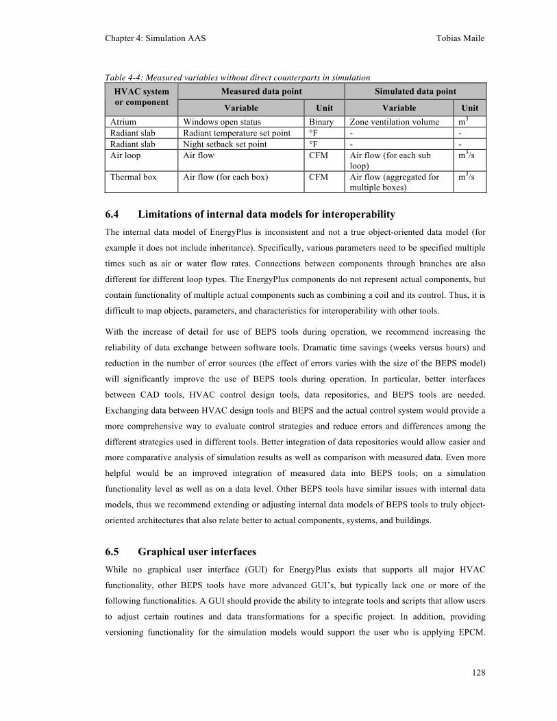
Chapter 4: Simulation AAS Tobias Maile
128
Table 4-4: Measured variables without direct counterparts in simulation Measured data point Simulated data point HVAC system
or component Variable Unit Variable Unit Atrium Windows open status Binary Zone ventilation volume m3 Radiant slab Radiant temperature set point °F - - Radiant slab Night setback set point °F - - Air loop Air flow CFM Air flow (for each sub
loop) m3/s
Thermal box Air flow (for each box) CFM Air flow (aggregated for multiple boxes)
m3/s
6.4 Limitations of internal data models for interoperability The internal data model of EnergyPlus is inconsistent and not a true object-oriented data model (for
example it does not include inheritance). Specifically, various parameters need to be specified multiple
times such as air or water flow rates. Connections between components through branches are also
different for different loop types. The EnergyPlus components do not represent actual components, but
contain functionality of multiple actual components such as combining a coil and its control. Thus, it is
difficult to map objects, parameters, and characteristics for interoperability with other tools.
With the increase of detail for use of BEPS tools during operation, we recommend increasing the
reliability of data exchange between software tools. Dramatic time savings (weeks versus hours) and
reduction in the number of error sources (the effect of errors varies with the size of the BEPS model)
will significantly improve the use of BEPS tools during operation. In particular, better interfaces
between CAD tools, HVAC control design tools, data repositories, and BEPS tools are needed.
Exchanging data between HVAC design tools and BEPS and the actual control system would provide a
more comprehensive way to evaluate control strategies and reduce errors and differences among the
different strategies used in different tools. Better integration of data repositories would allow easier and
more comparative analysis of simulation results as well as comparison with measured data. Even more
helpful would be an improved integration of measured data into BEPS tools; on a simulation
functionality level as well as on a data level. Other BEPS tools have similar issues with internal data
models, thus we recommend extending or adjusting internal data models of BEPS tools to truly object-
oriented architectures that also relate better to actual components, systems, and buildings.
6.5 Graphical user interfaces While no graphical user interface (GUI) for EnergyPlus exists that supports all major HVAC
functionality, other BEPS tools have more advanced GUI’s, but typically lack one or more of the
following functionalities. A GUI should provide the ability to integrate tools and scripts that allow users
to adjust certain routines and data transformations for a specific project. In addition, providing
versioning functionality for the simulation models would support the user who is applying EPCM.
Chapter 4: Simulation AAS Tobias Maile
129
Starting with the original design model, assessors will create a significant number of models that differ
mostly only in small aspects from each other. Providing versioning functionality could help the assessor
to maintain an overview of differences between models. In addition, a GUI should also allow for the use
of partial models, so the assessor can focus on specific aspects of a building without specifying the
detail of other parts of it. Enabling partial models would require creating adiabatic surfaces for the
needed geometry and summarizing and simplifying geometry, HVAC systems, and components.
Because of the current need to develop custom programming code that supports the energy modeler, we
recommend the development of a comprehensive GUI for EnergyPlus and other BEPS tools, to increase
the efficiency of model creation and updating.
6.6 Increased level of detail As reported in this paper, EnergyPlus does not always support the modeling of HVAC systems to the
level of detail needed for operation. This is a significant shortcoming and needs to be resolved. Besides
increasing the level of detail of HVAC components and possible topologies, simulation tools should
provide a range of HVAC components at different levels of complexity. This would enable the user to
start with a simple component model at early design stages and increase the complexity and level of
detail of the components over the course of design and into building operation. With increased detail,
the need for interoperability to exchange data also increases, as well as the need to manage the input
data, in particular the differences between different versions of BEPS models. Furthermore, increased
detail also requires modeling a wider variety of HVAC components, as well as new HVAC components
and HVAC system configurations, to match actual components and topologies more closely.
7 Validation of simulation AAS The value of simulation AAS is in their use in the EPCM, allowing the selection of more appropriate
BEPS tools, giving direction to their further development and allowing the construction of better BEPS
tools. Through AAS that are specific to BEPS tools, the AAS support the selection of an appropriate
BEPS tool for a given performance assessment scenario. The formalization of AAS highlights
limitations of BEPS tools and thus can direct future development efforts to overcome those limitations.
The documentation of AAS can also show fundamental problems with specific BEPS tools and thus
trigger new developments of BEPS tools to advance the tool development.
The validation is based on the performance problems found at the Y2E2 case study. Detailed
information about the performance problems is included in Maile et al. (2010b) and Kunz et al. (2009).
The former paper includes a prospective validation of the EPCM with the Y2E2 case study. In context
of this validation, AAS support the evaluation of differences between measured and simulated data. 41
differences between measured and simulated data could be explained with corresponding simulation
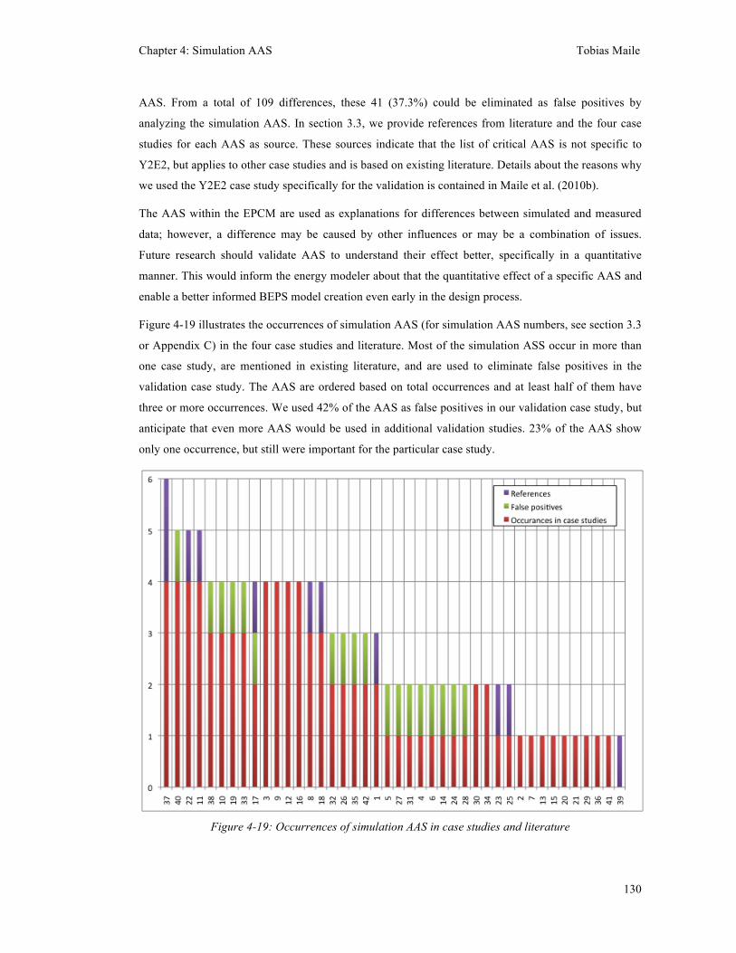
Chapter 4: Simulation AAS Tobias Maile
130
AAS. From a total of 109 differences, these 41 (37.3%) could be eliminated as false positives by
analyzing the simulation AAS. In section 3.3, we provide references from literature and the four case
studies for each AAS as source. These sources indicate that the list of critical AAS is not specific to
Y2E2, but applies to other case studies and is based on existing literature. Details about the reasons why
we used the Y2E2 case study specifically for the validation is contained in Maile et al. (2010b).
The AAS within the EPCM are used as explanations for differences between simulated and measured
data; however, a difference may be caused by other influences or may be a combination of issues.
Future research should validate AAS to understand their effect better, specifically in a quantitative
manner. This would inform the energy modeler about that the quantitative effect of a specific AAS and
enable a better informed BEPS model creation even early in the design process.
Figure 4-19 illustrates the occurrences of simulation AAS (for simulation AAS numbers, see section 3.3
or Appendix C) in the four case studies and literature. Most of the simulation ASS occur in more than
one case study, are mentioned in existing literature, and are used to eliminate false positives in the
validation case study. The AAS are ordered based on total occurrences and at least half of them have
three or more occurrences. We used 42% of the AAS as false positives in our validation case study, but
anticipate that even more AAS would be used in additional validation studies. 23% of the AAS show
only one occurrence, but still were important for the particular case study.
Figure 4-19: Occurrences of simulation AAS in case studies and literature

Chapter 4: Simulation AAS Tobias Maile
131
8 Limitations and future research This section describes limitations of this research and discusses possible future research areas based on
the concepts in this paper. In particular, we discuss emerging technologies in BEPS, an integration of
error calculations into BEPS, possible expert systems based on AAS and our process for identifying
performance problems, the limitations of the AAS list, and the possibility of detailed analysis of the
accuracy of simulation results. This research is a further step towards the application of BEPS tools to
predict the actual energy performance of buildings more accurately.
8.1 Emerging technologies in simulation tools Some new developments within the context of simulation tools can be integrated into the methodology.
In particular, while we selected and used a single simulation engine, it may prove beneficial to combine
two or more simulation tools to enable a more accurate model. Trcka et al. (2007) describe the coupling
of simulation tools as co-simulation research. Another similar approach enables communication among
multiple tools during execution time via sockets (Wetter and Haves 2008). This approach allows more
flexible use of tools that can model controls, such as Matlab or Simulink. Combining the functionality
of two or more simulation tools would allow taking advantage of the strengths of these tools and
helping to avoid their weaknesses. For example, the realistic simulation of controller signals in Matlab
connected to EnergyPlus would eliminate the difference due to time delays (or the lack thereof).
8.2 Integration of error calculations into whole building simulation tools Because of the complexity and large number of equations embedded in whole building simulation tools,
it is practically impossible to perform an error calculation outside of a simulation engine (see section
3.2). Future research could integrate error calculations into whole building simulation tools, so users
could specify error margins of input data and the tool would output error margins based on the input. In
addition to providing the error calculation in the tool, future research could also determine default error
margins and statistical sampling methods to better address the uncertainty of various input parameters
in the simulation. For example the solar radiation measurements (direct and diffuse) have various
effects on the performance of the building such as solar loads in spaces through windows but are often
measured crudely. The propagation of the error margin of the solar measurements would help to
understand the real influence of the accuracy of such a measurement. Though statistical sampling
methods the actual variation in building use could be modeled more realistically than with constant
values and regular patterns.
Chapter 4: Simulation AAS Tobias Maile
132
8.3 An expert system based on approximations, assumptions, and
simplifications Future research could define possible consequences of specific AAS and build an expert system that
automatically determines differences between measured and simulated data. Automated detection of
differences based on statistical criteria could highlight data pairs that show differences and simplify the
performance assessor’s task of finding data pairs that do not match. A second stage could use AAS to
qualify these differences as performance problems and provide indications of related performance
problems. Once both stages are mostly automated, the assessor could focus on the difficult data pairs
and save effort in finding these pairs in the first place. Performance problems could be found more
quickly and closer to their actual appearance. A quicker response time to find problems would enable
faster assessment of building energy performance and faster feedback on the BEPS models and their
AAS. This faster feedback would make a practical application more meaningful, since performance
problems can be determined in a more timely fashion.
8.4 Identifying new approximations, assumptions, and simplifications The list of critical AAS (see section 3.3) is based on literature review and the four case studies. Future
case studies and research may identify more AAS. New HVAC component models, system
configurations, and control strategies may require the definition of new AAS. In addition, the case study
models are all based on EnergyPlus. The limitations of EnergyPlus may not correspond to those in other
BEPS tools, and thus new AAS may need to be added to the list to account for specific concepts in
other BEPS tools. The development of new assumptions and their anticipated effect as well as a
hierarchy of AAS based on their anticipated effect would depend on future tool developments and
typical modeling practice. The anticipated effect of each AAS is also an area of further research. The
validation of these effects and more stringent descriptions would aid the development of an expert
system.
8.5 Detailed analysis of accuracy of simulation results A detailed quantitative investigation of accuracy of simulation results was beyond the scope of this
research; however, future research could integrate accuracy calculations, either within the BEPS tool or
within the EPCM. Assessing accuracy of measured and simulated data could provide a more reliable
assessment of differences between measured and simulated data. Developing more accurate simulation
results will reduce the number of AAS needed to document limitations and make the process of EPCM
easier.
Chapter 4: Simulation AAS Tobias Maile
133
9 Conclusion
In this paper, we provide a list and categorization of critical simulation AAS we collected from
literature research and experience with four case studies. These AAS describe limitations of BEPS
models, in particular limitations of input data, use of simulation concepts, and shortcomings of BEPS
tools (specifically EnergyPlus). This list and the process for using AAS to determine performance
problems are new concepts and thus contributions of this paper. These simulation AAS enable a better
assessment of differences between measured and simulated data.
We selected EnergyPlus as the most suitable simulation engine; based on the requirements we
developed for a comparison between measured and simulated data. Specifically, EnergyPlus’ ability to
communicate with control design tools and to generate partial geometry models, as well as the
reasonable set of available HVAC components, are key characteristics that differentiate it from other
BEPS tools. To properly transition design BEPS tools into operation, these tools need further
adjustments. We have described shortcomings and limitations of simulation tools (in particular
EnergyPlus) and have given our recommendations for future developments. Specifically, requiring
simulation tools to enable more data exchange would enhance the use of performance evaluation based
on design models. In addition, improved data exchange would support reuse of design data more
directly and reduce the effort needed to generate or update BEPS models. We have recommended that
BEPS tools increase their level of detail to correspond to the level of detail of actual buildings. We have
also discussed additional possible improvements to EnergyPlus related to comparing simulation data
with measured data in terms of model warm-up, making more report variables available, and improving
the functionality for importing measured data. We have discussed limitations of this research and future
research directions. This research provides a step towards enabling prediction of actual building
performance.
10 Bibliography Approximation. (2010). In Cambridge dictionaries online. http://dictionary.cambridge.org/ last accessed
on May 23, 2010.
Assumption. (2010). In Merriam Webster’s online dictionary. http://www.merriam-webster.com/ last
accessed on May 23, 2010.
Bazjanac, V. (2001). Acquisition of building geometry in the simulation of energy performance.
Proceedings of the Seventh International IBPSA Conference, 305–311. Rio de Janeiro, Brazil:
International Building Performance Simulation Association (IBPSA).

Chapter 4: Simulation AAS Tobias Maile
134
Bazjanac, V. (2005). Model based cost and energy performance estimation during schematic design.
Proceedings of the 22nd Conference on Information Technology in Construction, 677-688.
Dresden: Institute for Construction Informatics, Technische Universitaet Dresden.
Bazjanac, V. (2008). IFC BIM-based methodology for semi-automated building energy performance
simulation. Berkeley, CA: Lawrence Berkeley National Laboratory.
http://escholarship.org/uc/item/0m8238pj last accessed on March 31, 2010.
Bensouda, N. (2004). Extending and formalizing the energy signature method for calibrating
simulations and illustrating with application for three California climates. Master Thesis,
College Station, TX: Texas A&M University.
buildingSMART. (2010). buildingSMART. http://www.buildingsmart.com/ last accessed on February
26, 2010.
Carrilho da Graca, G., P.F. Linden, and P. Haves. (2004). Design and testing of a control strategy for a
large naturally ventilated office building. Building Services Engineering Research and
Technology, 25(3), 223–239.
Corrado, V., and H.E. Mechri. (2009). Uncertainty and sensitivity analysis for building energy rating.
Journal of Building Physics, 33(2), 125-156.
Crawley, D.B., J.W. Hand, S. Glasgow, U.K. Kummert, and B.T. Griffith. (2005). Contrasting the
capabilities of building energy performance simulation programs. Joint Report. US Dept of
Energy, University of Strathclyde, University of Wisconsin and National Renewable Energy
Laboratory (NREL).
Crawley, D.B., J.W. Hand, M. Kummert, and B.T. Griffith. (2008). Contrasting the capabilities of
building energy performance simulation programs. Building and Environment (April), 43(4),
661-673.
De Wit, S., and G. Augenbroe. (2002). Analysis of uncertainty in building design evaluations and its
implications. Energy and Buildings, 34(9), 951–958.
Duffie, J.A., and W.A. Beckman. (1980). Solar engineering of thermal processes. New York, NY: John
Wiley & Sons.
EETD. (2003). COMIS multizone air flow model. http://epb.lbl.gov/comis/ last accessed on March 11,
2010.
Ellis, P.G., P.A. Torcellini, and D.B. Crawley. (2007). Simulation of energy management systems in
EnergyPlus. Proceedings of the 10th International IBPSA Conference, 1346-1353. Beijing,
China: International Building Performance Simulation Association (IBPSA).

Chapter 4: Simulation AAS Tobias Maile
135
Energy Design Resources. (2005). Design guidelines: HVAC simulation guidelines - Volume I.
http://www.energydesignresources.com/Portals/0/documents/DesignGuidelines/EDR_DesignG
uidelines_%20HVAC_Simulation.pdf last accessed on May 21, 2008.
Esmore, S. (2005). Innovative design - BATISO and night sky cooling. EcoLibrium - AIRAH Journal,
4(8), 30-35.
Ferson, S., W.L. Oberkampf, and L. Ginzburg. (2008). Model validation and predictive capability for
the thermal challenge problem. Computer Methods in Applied Mechanics and Engineering
(May 1), 197(29-32), 2408-2430. doi:10.1016/j.cma.2007.07.030.
Fong, K., C. Lee, T. Chow, Z. Lin, and L. Chan. (2010). Solar hybrid air-conditioning system for high
temperature cooling in subtropical city. Renewable Energy, 35(11), 2439-2451.
doi:10.1016/j.renene.2010.02.024.
Ganeshan, R., L. Johnson, and R. Henderson. (1999). Automated diagnosis for facility HVAC systems.
Technical Report #99. Menlo Park, CA: Association for the Advancement of Artificial
Intelligence.
Gowri, K., D. Winiarski, and R. Jarnagin. (2009). Infiltration modeling guidelines for commercial
building energy analysis. PNNL #18898. Richland, WA: Pacific Northwest National
Laboratory.
GSA. (2009). GSA Building Information Modeling Series 05 - Energy Performance DRAFT.
http://www.gsa.gov/graphics/pbs/GSA_BIM_Guide_Series_05_Version_1.pdf last accessed
on July 8, 2010.
Hensen, J.L.M., and J.A. Clarke. (2000). Integrated simulation for HVAC performance prediction:
state-of-the-art illustration. Proceedings of the International ASHRAE/CIBSE Conference.
Dublin, Ireland: American Society of Heating, Refrigerating and Air-Conditioning Engineers
(ASHRAE).
Holst, J.N. (2003). Using whole building simulation models and optimizing procedures to optimize
building envelope design with respect to energy consumption and indoor environment.
Proceedings of the Eighth International IBPSA Conference, 507–514. Eindhoven, Netherlands:
International Building Performance Simulation Association (IBPSA).
IPMVP Committee. (2002). International performance measurement and verification protocol -
Concepts and Options for Determining Energy and Water Savings. Technical Report #810.
Golden, CO: National Renewable Energy Laboratory.
Klote, J.H. (1988). A computer model of smoke movement by air conditioning systems (SMACS). Fire
Technology, 24(4), 299–311.

Chapter 4: Simulation AAS Tobias Maile
136
Kunz, J., T. Maile, and V. Bazjanac. (2009). Summary of the energy analysis of the first year of the
Stanford Jerry Yang & Akiko Yamazaki Environment & Energy (Y2E2) Building. Technical
Report #183. Stanford, CA: Center for Integrated Facility Engineering, Stanford University.
http://cife.stanford.edu/online.publications/TR183.pdf last accessed on March 15, 2010.
LBNL. (2010). HVAC graphical user interface (GUI) for Energy Plus project. under development:
being developed by Lawrence Berkeley National Laboratory and Infosys; funded by U.S.
Department of Energy and California Energy Commission.
Li, S. (2009). A model-based fault detection and diagnostic methodology for secondary HVAC systems.
Ph.D. Thesis, Philadelphia, PA: Drexel University.
Mackay, K. (2007). Energy efficient cooling solutions for data centres. Master thesis, Glasgow,
Scotland: University of Strathclyde.
Maile, T., M. Fischer, and V. Bazjanac. (2007a). Building energy performance simulation tools-a life-
cycle and interoperable perspective. Working Paper #107. Stanford, CA: Center for Integrated
Facility Engineering, Stanford University.
http://cife.stanford.edu/online.publications/WP107.pdf last accessed on April 4, 2010.
Maile, T., M. Fischer, and R. Huijbregts. (2007b). The vision of integrated IP-based building systems.
Journal of Corporate Real Estate, 9(2), 125–137.
Maile, T., M. Fischer, and V. Bazjanac. (2010a). A method to compare measured and simulated
building energy performance data. Working Paper #127. Stanford, CA: Center for Integrated
Facility Engineering, Stanford University.
Maile, T., M. Fischer, and V. Bazjanac. (2010b). Formalizing assumptions to document limitations of
building performance measurement systems. Working Paper #125. Stanford, CA: Center for
Integrated Facility Engineering, Stanford University.
Modelica. (2010). Modelica and the Modelica Association — Modelica Portal.
http://www.modelica.org/ last accessed on July 22, 2010.
Morrison, L., R. Azerbegi, and A. Walker. (2008). Energy modeling for measurement and verification.
Proceedings of the 3rd National Conference of IBPSA-USA, 17-22. Berkeley, CA:
International Building Performance Simulation Association (IBPSA).
Morrissey, E. (2006). Building effectiveness communication ratios (BECs): An integrated life-cycle
methodology for mitigating energy-use in buildings. Ph.D. Thesis, Cork, Ireland: University
College Cork (UCC).
Pati, D., C.S. Park, and G. Augenbroe. (2006). Roles of building performance assessment in stakeholder
dialogue in AEC. Automation in Construction, 15(4), 415–427.

Chapter 4: Simulation AAS Tobias Maile
137
Rauscher, S., H. Wu, M.A. Hunter, and C.J. Williams. (2002). Pressure measurements at natural
ventilation study - New San Francisco Federal Office Building. Technical Report. San
Francisco: Rowan Williams Davis & Irwin Inc.
Simplification. (2010). In Cambridge dictionaries online. http://dictionary.cambridge.org/ last accessed
on May 23, 2010.
Suwon, S. (2007). Development of New Methodologies for Evaluating the Energy Performance of New
Commercial Buildings. Ph.D. Thesis, College Station, TX: Texas A&M University.
http://handle.tamu.edu/1969.1/6056 last accessed on October 26, 2009.
Trcka, M., and J. Hensen. (2009). Overview of HVAC system simulation. Automation in Construction,
19(2), 93-99.
Trcka, M., M. Wetter, and J. Hensen. (2007). Comparison of co-simulation approaches for building and
HVAC/R system simulation. Proceedings of the Building Simulation 2007, 1418-1425.
Beijing, China: International Building Performance Simulation Association (IBPSA).
Turner, C., and M. Frankel. (2008). Energy performance of LEED® for new construction buildings.
Vancouver, WA: New Building Institute.
U.S. DOE. (2010a). Building technologies program: Building energy software tools directory.
http://apps1.eere.energy.gov/buildings/tools_directory/ last accessed on February 15, 2010.
U.S. DOE. (2010b). Auxiliary EnergyPlus programs. University of Illinois and Lawrence Berkeley
National Laboratory.
http://apps1.eere.energy.gov/buildings/energyplus/pdfs/auxiliaryprograms.pdf last accessed on
February 27, 2010.
U.S. DOE. (2010c). EnergyPlus - Input Output reference.
http://apps1.eere.energy.gov/buildings/energyplus/pdfs/inputoutputreference.pdf last accessed
on May 21, 2010.
U.S. DOE. (2010d). EnergyPlus - Engineering reference.
http://apps1.eere.energy.gov/buildings/energyplus/pdfs/engineeringreference.pdf last accessed
on May 21, 2010.
U.S. DOE. (2010e). EnergyPlus: Feature highlights.
http://apps1.eere.energy.gov/buildings/energyplus/features.cfm last accessed on May 24, 2010.
Wetter, M., and P. Haves. (2008). A modular building controls virtual test bed for the integration of
heterogeneous systems. Proceedings of SimBuild 2008, 69–76. Berkeley, CA: International
Building Performance Simulation Association (IBPSA).

Chapter 4: Simulation AAS Tobias Maile
138
Xu, P., P. Haves, and K. Moosung. (2005). A semi-automated functional test data analysis tool.
Proceedings of the 13th National Conference on Building Commissioning. New York City,
NY: Portland Energy Conservation Inc (PECI).
Yin, R.K. (2003). Case study research: Design and methods. 3rd ed. Thousand Oaks, CA: Sage
Publications.

Appendix Tobias Maile
139
Appendix A: Details about the analysis of measurement data sets The first step in our method of validating existing measurement data sets (see chapter 3 section 5.1) is
to determine which sensors are needed to detect each problem from the known performance problem set
of Y2E2 (see Table A-1).
Table A-1: Necessary sensors to detect known performance problems Known performance problems Needed sensors
No. Description Count Description 1 Hot water flow rate stays constant even though valve
position changes 2 Hot water flow rate and
valve position 2 Radiant slab valve position is only 0 or 100% open
(should change in increments) 6 Radiant slab valve position
and temperatures 3 Current draw shows integer values only 1 Space level electricity
meter 4 Sum of electrical sub meters << total electricity
consumption 26 Total and electrical sub
meters 5 Active beam hot water supply and return water temp
are reverse 3 Active beam supply and
return temperature and flow rate
6 Active beam hot water temps are inconsistent with hot water system temp
2 System and component level water temp
7 Chilled water valve position does not fully correlate with chilled water flow
2 Chilled water valve position and flow
8 Temperature values out of range (725 deg F) 1 Temperature sensor 9 Pressure values out of range (e.g., 600 psi) 1 Pressure sensor
10 Minimum flow rate is 1 GPM 1 Flow rate sensor 11 Heating coil valve cycles open and closed rapidly 3 Heating coil valve,
temperatures 12 Heat recovery bypass valve opens and closes rapidly
during transitional periods 5 HR valve, HR
temperatures 13 Night purge on the 1st and 2nd floor is on a regular
schedule rather than dependent on temperatures 3 Window status, indoor
outdoor temperatures 14 Night purge on 3rd floor seems random and does not
follow control strategy 3 Window status, indoor
outdoor temperatures 15 Radiant slab control valve position does not show step
behavior as outlined in sequence of operations 6 Radiant slab valve position
and temperatures 16 Heat recovery cooling mode does not coincide with
coil cooling mode at all times 5 HR valve, HR
temperatures 17 Occupancy schedules differ (5 day work week -> 7
day work week) 10 Electrical submeters plug
loads 18 Fan coil unit capacity not sufficient 3 Space temp, cooling coil
valve and fan status 19 Hot water loop set point differs (150 instead of 180) 1 Hot water loop set point 20 Server room included in the model 4 Supply and return water
temp and 2 pump speeds
Based on these necessary sensors, I determined which of them is available in each one of the four
measurement data set guidelines (see Table A-2).
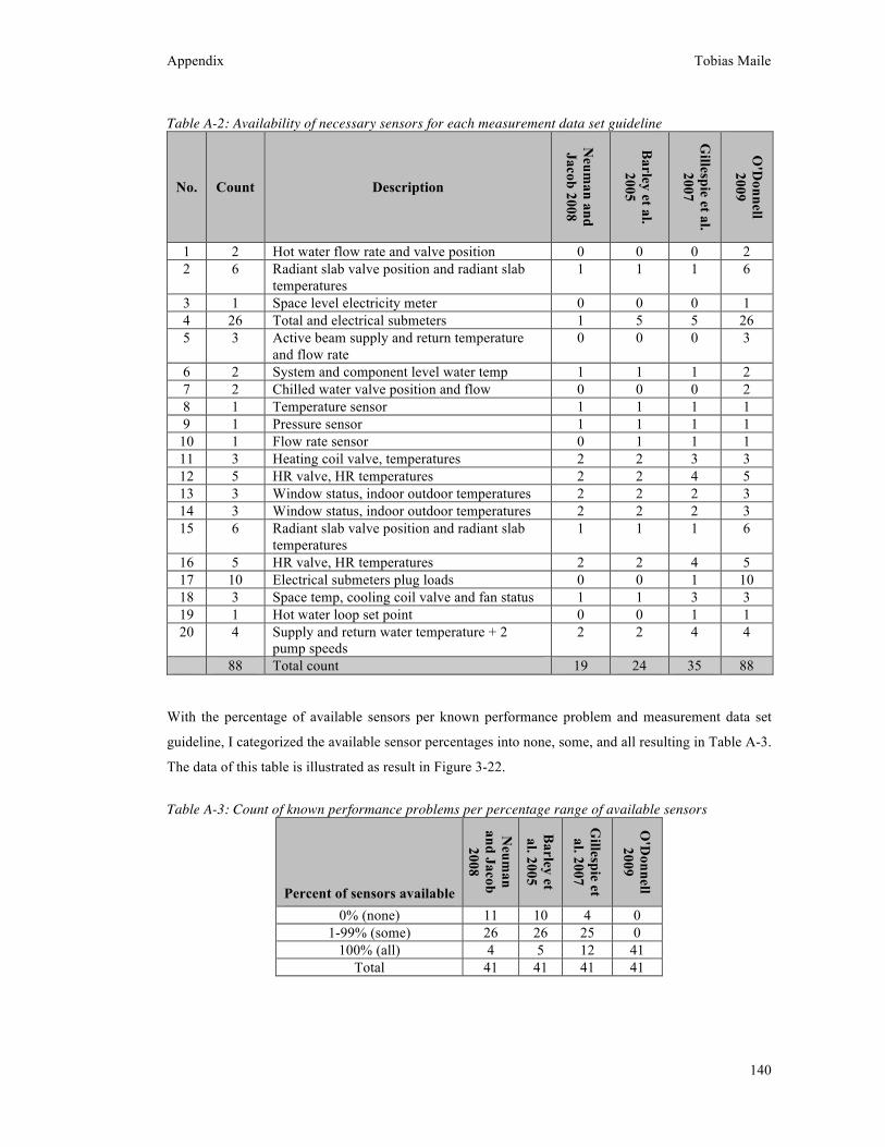
Appendix Tobias Maile
140
Table A-2: Availability of necessary sensors for each measurement data set guideline
No. Count Description
Neum
an and Jacob 2008
Barley et al.
2005
Gillespie et al.
2007
O'D
onnell 2009
1 2 Hot water flow rate and valve position 0 0 0 2 2 6 Radiant slab valve position and radiant slab
temperatures 1 1 1 6
3 1 Space level electricity meter 0 0 0 1 4 26 Total and electrical submeters 1 5 5 26 5 3 Active beam supply and return temperature
and flow rate 0 0 0 3
6 2 System and component level water temp 1 1 1 2 7 2 Chilled water valve position and flow 0 0 0 2 8 1 Temperature sensor 1 1 1 1 9 1 Pressure sensor 1 1 1 1
10 1 Flow rate sensor 0 1 1 1 11 3 Heating coil valve, temperatures 2 2 3 3 12 5 HR valve, HR temperatures 2 2 4 5 13 3 Window status, indoor outdoor temperatures 2 2 2 3 14 3 Window status, indoor outdoor temperatures 2 2 2 3 15 6 Radiant slab valve position and radiant slab
temperatures 1 1 1 6
16 5 HR valve, HR temperatures 2 2 4 5 17 10 Electrical submeters plug loads 0 0 1 10 18 3 Space temp, cooling coil valve and fan status 1 1 3 3 19 1 Hot water loop set point 0 0 1 1 20 4 Supply and return water temperature + 2
pump speeds 2 2 4 4
88 Total count 19 24 35 88
With the percentage of available sensors per known performance problem and measurement data set
guideline, I categorized the available sensor percentages into none, some, and all resulting in Table A-3.
The data of this table is illustrated as result in Figure 3-22.
Table A-3: Count of known performance problems per percentage range of available sensors
Percent of sensors available
Neum
an and Jacob
2008
Barley et
al. 2005
Gillespie et al. 2007
O'D
onnell 2009
0% (none) 11 10 4 0 1-99% (some) 26 26 25 0
100% (all) 4 5 12 41 Total 41 41 41 41
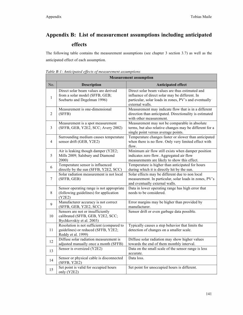
Appendix Tobias Maile
141
Appendix B: List of measurement assumptions including anticipated
effects The following table contains the measurement assumptions (see chapter 3 section 3.7) as well as the
anticipated effect of each assumption.
Table B-1: Anticipated effects of measurement assumptions Measurement assumption
No. Description Anticipated effect
1
Direct solar beam values are derived from a solar model (SFFB, GEB; Soebarto and Degelman 1996)
Direct solar beam values are thus estimated and influence of direct solar may be different. In particular, solar loads in zones, PV’s and eventually external walls.
2 Measurement is one-dimensional (SFFB)
Measurement may indicate flow that is in a different direction than anticipated. Directionality is estimated with other measurement.
3 Measurement is a spot measurement (SFFB, GEB, Y2E2, SCC; Avery 2002)
Measurement may not be comparable in absolute terms, but also relative changes may be different for a single point versus average points.
4 Surrounding medium causes temperature sensor drift (GEB, Y2E2)
Temperature changes faster or slower than anticipated when there is no flow. Only very limited effect with flow.
5 Air is leaking though damper (Y2E2; Mills 2009; Salsbury and Diamond 2000)
Minimum air flow still exists when damper position indicates zero flow. Aggregated air flow measurements are likely to show this effect.
6 Temperature sensor is influenced directly by the sun (SFFB, Y2E2, SCC)
Temperature is higher than anticipated for hours during which it is directly hit by the sun.
7 Solar radiation measurement is not local (SFFB, GEB)
Solar effects may be different due to non local measurement. In particular, solar loads in zones, PV’s and eventually external walls.
8 Sensor operating range is not appropriate (following guidelines) for application (Y2E2)
Data in lower operating range has high error that needs to be considered.
9 Manufacturer accuracy is not correct (SFFB, GEB, Y2E2, SCC)
Error margins may be higher than provided by manufacturer.
10 Sensors are not or insufficiently calibrated (SFFB, GEB, Y2E2, SCC; Bychkovskiy et al. 2003)
Sensor drift or even garbage data possible.
11 Resolution is not sufficient (compared to guidelines) or reduced (SFFB, Y2E2; Reddy et al. 1999)
Typically causes a step behavior that limits the detection of changes on a smaller scale.
12 Diffuse solar radiation measurement is adjusted manually once a month (SFFB)
Diffuse solar radiation may show higher values towards the end of them monthly interval.
13 Sensor is oversized (Y2E2) Data on the small scale of the sensor range is less accurate.
14 Sensor or physical cable is disconnected (SFFB, Y2E2)
Data loss.
15 Set point is valid for occupied hours only (Y2E2)
Set point for unoccupied hours is different.
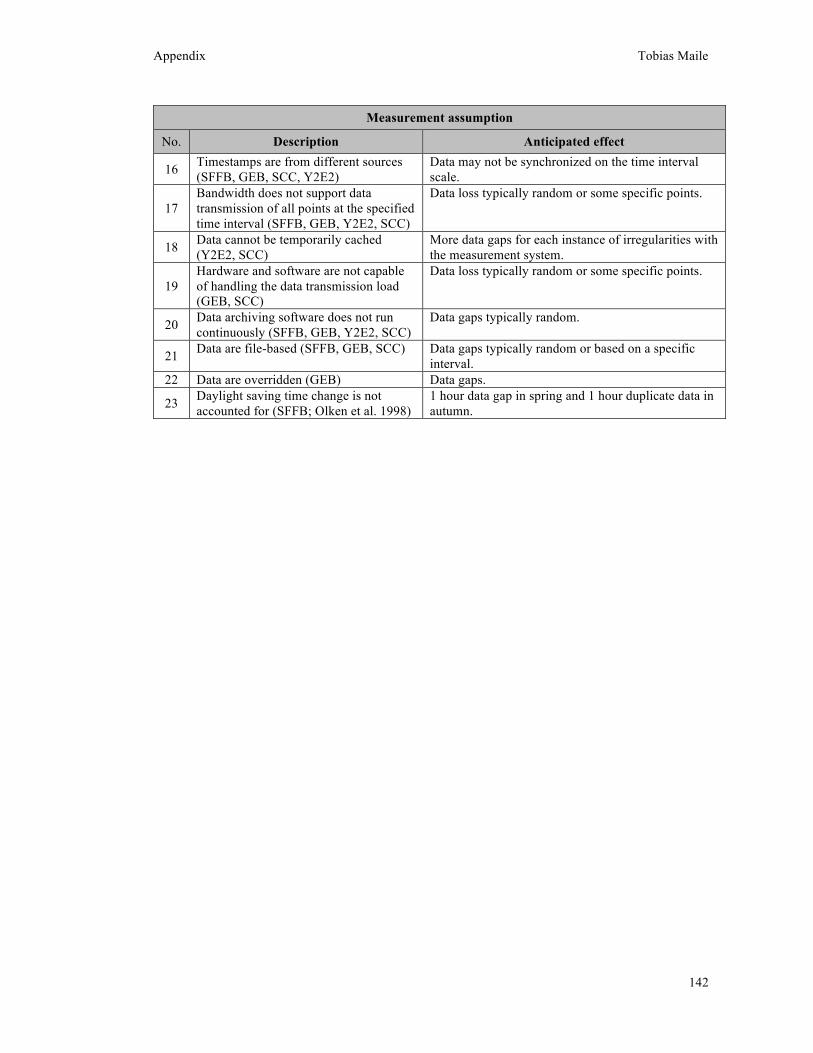
Appendix Tobias Maile
142
Measurement assumption
No. Description Anticipated effect
16 Timestamps are from different sources (SFFB, GEB, SCC, Y2E2)
Data may not be synchronized on the time interval scale.
17 Bandwidth does not support data transmission of all points at the specified time interval (SFFB, GEB, Y2E2, SCC)
Data loss typically random or some specific points.
18 Data cannot be temporarily cached (Y2E2, SCC)
More data gaps for each instance of irregularities with the measurement system.
19 Hardware and software are not capable of handling the data transmission load (GEB, SCC)
Data loss typically random or some specific points.
20 Data archiving software does not run continuously (SFFB, GEB, Y2E2, SCC)
Data gaps typically random.
21 Data are file-based (SFFB, GEB, SCC) Data gaps typically random or based on a specific interval.
22 Data are overridden (GEB) Data gaps.
23 Daylight saving time change is not accounted for (SFFB; Olken et al. 1998)
1 hour data gap in spring and 1 hour duplicate data in autumn.
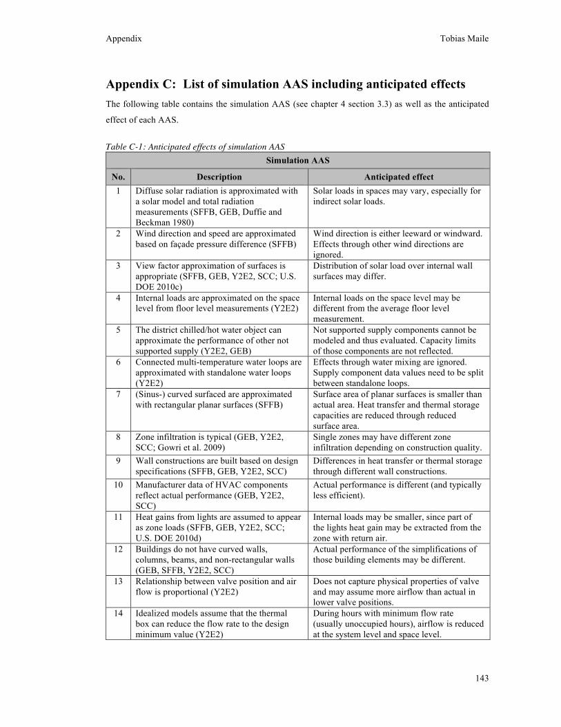
Appendix Tobias Maile
143
Appendix C: List of simulation AAS including anticipated effects The following table contains the simulation AAS (see chapter 4 section 3.3) as well as the anticipated
effect of each AAS.
Table C-1: Anticipated effects of simulation AAS Simulation AAS
No. Description Anticipated effect 1 Diffuse solar radiation is approximated with
a solar model and total radiation measurements (SFFB, GEB, Duffie and Beckman 1980)
Solar loads in spaces may vary, especially for indirect solar loads.
2 Wind direction and speed are approximated based on façade pressure difference (SFFB)
Wind direction is either leeward or windward. Effects through other wind directions are ignored.
3 View factor approximation of surfaces is appropriate (SFFB, GEB, Y2E2, SCC; U.S. DOE 2010c)
Distribution of solar load over internal wall surfaces may differ.
4 Internal loads are approximated on the space level from floor level measurements (Y2E2)
Internal loads on the space level may be different from the average floor level measurement.
5 The district chilled/hot water object can approximate the performance of other not supported supply (Y2E2, GEB)
Not supported supply components cannot be modeled and thus evaluated. Capacity limits of those components are not reflected.
6 Connected multi-temperature water loops are approximated with standalone water loops (Y2E2)
Effects through water mixing are ignored. Supply component data values need to be split between standalone loops.
7 (Sinus-) curved surfaced are approximated with rectangular planar surfaces (SFFB)
Surface area of planar surfaces is smaller than actual area. Heat transfer and thermal storage capacities are reduced through reduced surface area.
8 Zone infiltration is typical (GEB, Y2E2, SCC; Gowri et al. 2009)
Single zones may have different zone infiltration depending on construction quality.
9 Wall constructions are built based on design specifications (SFFB, GEB, Y2E2, SCC)
Differences in heat transfer or thermal storage through different wall constructions.
10 Manufacturer data of HVAC components reflect actual performance (GEB, Y2E2, SCC)
Actual performance is different (and typically less efficient).
11 Heat gains from lights are assumed to appear as zone loads (SFFB, GEB, Y2E2, SCC; U.S. DOE 2010d)
Internal loads may be smaller, since part of the lights heat gain may be extracted from the zone with return air.
12 Buildings do not have curved walls, columns, beams, and non-rectangular walls (GEB, SFFB, Y2E2, SCC)
Actual performance of the simplifications of those building elements may be different.
13 Relationship between valve position and air flow is proportional (Y2E2)
Does not capture physical properties of valve and may assume more airflow than actual in lower valve positions.
14 Idealized models assume that the thermal box can reduce the flow rate to the design minimum value (Y2E2)
During hours with minimum flow rate (usually unoccupied hours), airflow is reduced at the system level and space level.
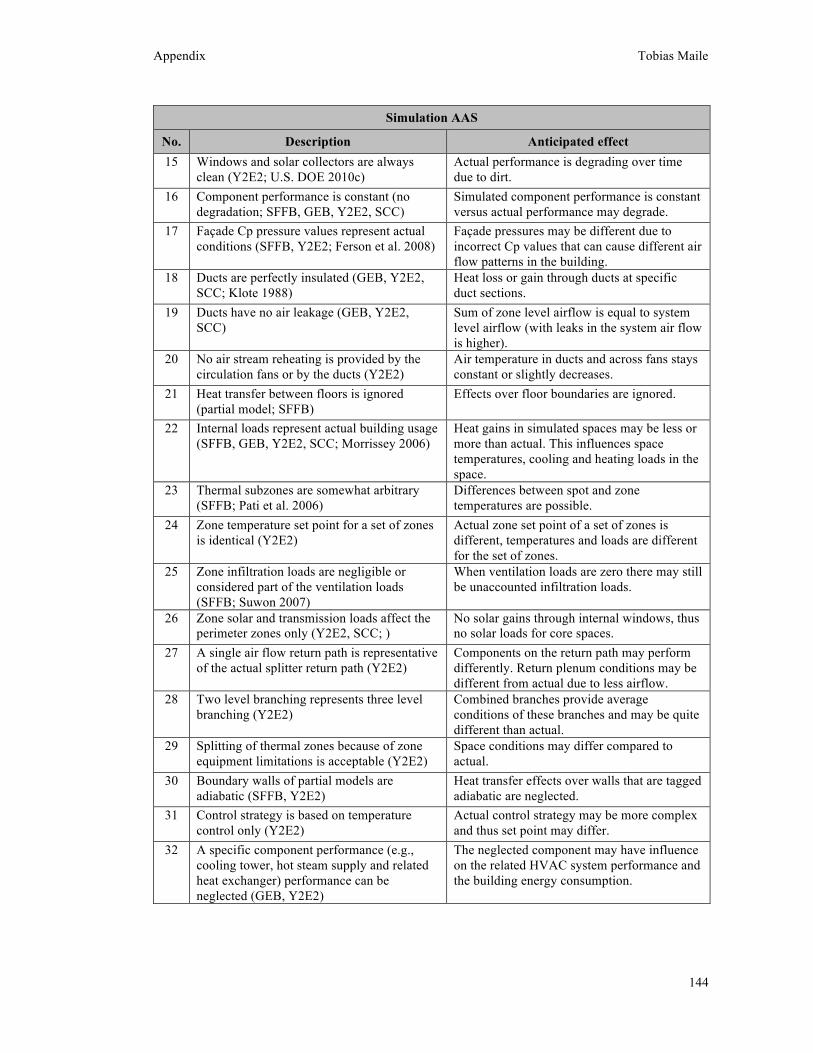
Appendix Tobias Maile
144
Simulation AAS
No. Description Anticipated effect 15 Windows and solar collectors are always
clean (Y2E2; U.S. DOE 2010c) Actual performance is degrading over time due to dirt.
16 Component performance is constant (no degradation; SFFB, GEB, Y2E2, SCC)
Simulated component performance is constant versus actual performance may degrade.
17 Façade Cp pressure values represent actual conditions (SFFB, Y2E2; Ferson et al. 2008)
Façade pressures may be different due to incorrect Cp values that can cause different air flow patterns in the building.
18 Ducts are perfectly insulated (GEB, Y2E2, SCC; Klote 1988)
Heat loss or gain through ducts at specific duct sections.
19 Ducts have no air leakage (GEB, Y2E2, SCC)
Sum of zone level airflow is equal to system level airflow (with leaks in the system air flow is higher).
20 No air stream reheating is provided by the circulation fans or by the ducts (Y2E2)
Air temperature in ducts and across fans stays constant or slightly decreases.
21 Heat transfer between floors is ignored (partial model; SFFB)
Effects over floor boundaries are ignored.
22 Internal loads represent actual building usage (SFFB, GEB, Y2E2, SCC; Morrissey 2006)
Heat gains in simulated spaces may be less or more than actual. This influences space temperatures, cooling and heating loads in the space.
23 Thermal subzones are somewhat arbitrary (SFFB; Pati et al. 2006)
Differences between spot and zone temperatures are possible.
24 Zone temperature set point for a set of zones is identical (Y2E2)
Actual zone set point of a set of zones is different, temperatures and loads are different for the set of zones.
25 Zone infiltration loads are negligible or considered part of the ventilation loads (SFFB; Suwon 2007)
When ventilation loads are zero there may still be unaccounted infiltration loads.
26 Zone solar and transmission loads affect the perimeter zones only (Y2E2, SCC; )
No solar gains through internal windows, thus no solar loads for core spaces.
27 A single air flow return path is representative of the actual splitter return path (Y2E2)
Components on the return path may perform differently. Return plenum conditions may be different from actual due to less airflow.
28 Two level branching represents three level branching (Y2E2)
Combined branches provide average conditions of these branches and may be quite different than actual.
29 Splitting of thermal zones because of zone equipment limitations is acceptable (Y2E2)
Space conditions may differ compared to actual.
30 Boundary walls of partial models are adiabatic (SFFB, Y2E2)
Heat transfer effects over walls that are tagged adiabatic are neglected.
31 Control strategy is based on temperature control only (Y2E2)
Actual control strategy may be more complex and thus set point may differ.
32 A specific component performance (e.g., cooling tower, hot steam supply and related heat exchanger) performance can be neglected (GEB, Y2E2)
The neglected component may have influence on the related HVAC system performance and the building energy consumption.
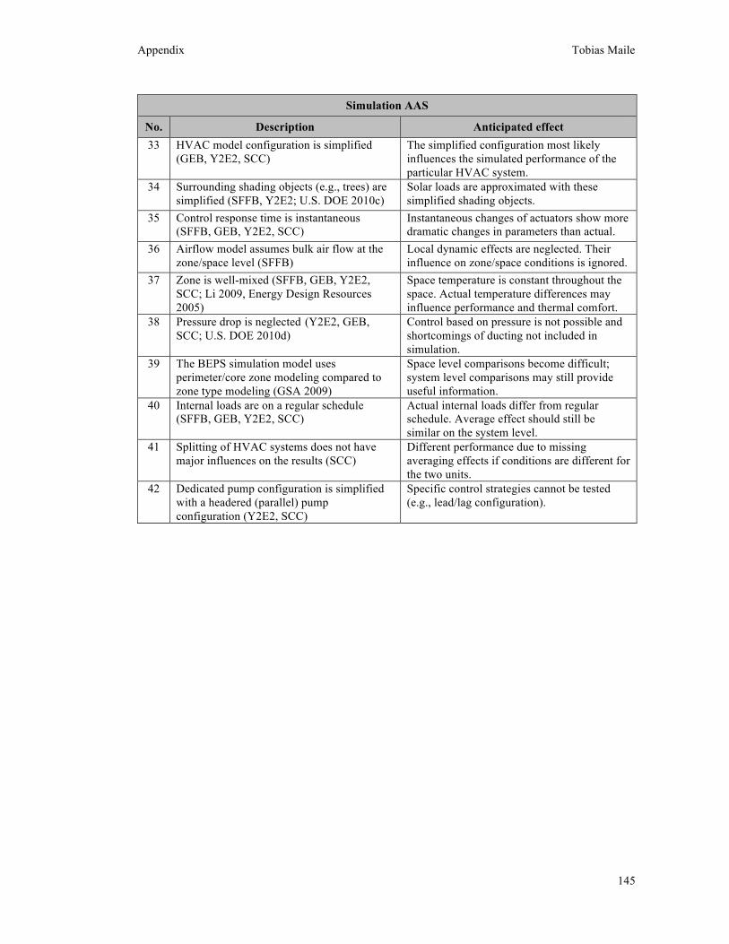
Appendix Tobias Maile
145
Simulation AAS
No. Description Anticipated effect 33 HVAC model configuration is simplified
(GEB, Y2E2, SCC) The simplified configuration most likely influences the simulated performance of the particular HVAC system.
34 Surrounding shading objects (e.g., trees) are simplified (SFFB, Y2E2; U.S. DOE 2010c)
Solar loads are approximated with these simplified shading objects.
35 Control response time is instantaneous (SFFB, GEB, Y2E2, SCC)
Instantaneous changes of actuators show more dramatic changes in parameters than actual.
36 Airflow model assumes bulk air flow at the zone/space level (SFFB)
Local dynamic effects are neglected. Their influence on zone/space conditions is ignored.
37 Zone is well-mixed (SFFB, GEB, Y2E2, SCC; Li 2009, Energy Design Resources 2005)
Space temperature is constant throughout the space. Actual temperature differences may influence performance and thermal comfort.
38 Pressure drop is neglected (Y2E2, GEB, SCC; U.S. DOE 2010d)
Control based on pressure is not possible and shortcomings of ducting not included in simulation.
39 The BEPS simulation model uses perimeter/core zone modeling compared to zone type modeling (GSA 2009)
Space level comparisons become difficult; system level comparisons may still provide useful information.
40 Internal loads are on a regular schedule (SFFB, GEB, Y2E2, SCC)
Actual internal loads differ from regular schedule. Average effect should still be similar on the system level.
41 Splitting of HVAC systems does not have major influences on the results (SCC)
Different performance due to missing averaging effects if conditions are different for the two units.
42 Dedicated pump configuration is simplified with a headered (parallel) pump configuration (Y2E2, SCC)
Specific control strategies cannot be tested (e.g., lead/lag configuration).


![huniv.hongik.ac.krhuniv.hongik.ac.kr/~hschoo/images/publication... · 2018-05-21 · [5]). The measured and simulated results are plotted as solid and dashed lines, respectively,](https://img.pdfslide.us/doc/110x75/5edbd223ad6a402d6666391a/huniv-hschooimagespublication-2018-05-21-5-the-measured-and-simulated.jpg)


![Mode Conversion, Current Drive and Flow Drive with High ... · [x10 17 m-2] ~ Simulated Channel. Electron Power Deposition Profile: Measured and Simulated Measured power deposition](https://img.pdfslide.us/doc/110x75/5c13729809d3f224238c8267/mode-conversion-current-drive-and-flow-drive-with-high-x10-17-m-2-simulated.jpg)