HAL Id: halshs-00805751https://halshs.archives-ouvertes.fr/halshs-00805751

Submitted on 28 Mar 2013

HAL is a multi-disciplinary open accessarchive for the deposit and dissemination of sci-entific research documents, whether they are pub-lished or not. The documents may come fromteaching and research institutions in France orabroad, or from public or private research centers.

L’archive ouverte pluridisciplinaire HAL, estdestinée au dépôt et à la diffusion de documentsscientifiques de niveau recherche, publiés ou non,émanant des établissements d’enseignement et derecherche français ou étrangers, des laboratoirespublics ou privés.

Comparing Inequality Aversion across Countries WhenLabor Supply Responses Differ

Olivier Bargain, Mathias Dolls, Dirk Neumann, Andreas Peichl, SebastianSiegloch

To cite this version:Olivier Bargain, Mathias Dolls, Dirk Neumann, Andreas Peichl, Sebastian Siegloch. Comparing In-equality Aversion across Countries When Labor Supply Responses Differ. 2013. �halshs-00805751�

Working Papers / Documents de travail

WP 2013 - Nr 23

Comparing Inequality Aversion across Countries When Labor Supply Responses Differ

Olivier BargainMathias Dolls

Dirk NeumannAndreas Peichl

Sebastian Siegloch

Comparing Inequality Aversion across Countries

When Labor Supply Responses Di¤er�

Olivier Bargain, Mathias Dolls, Dirk Neumann,Andreas Peichl, Sebastian Siegloch

Submitted in May 2012, accepted in March 2013,forthcoming in International Tax and Public Finance

Abstract

We analyze to which extent social inequality aversion di¤ers across nations when control-ling for actual country di¤erences in labor supply responses. Towards this aim, we estimatelabor supply elasticities at both extensive and intensive margins for 17 EU countries andthe US. Using the same data, inequality aversion is measured as the degree of redistribu-tion implicit in current tax-bene�t systems, when these systems are deemed optimal. We�nd relatively small di¤erences in labor supply elasticities across countries. However, thischanges the cross-country ranking in inequality aversion compared to scenarios following thestandard approach of using uniform elasticities. Di¤erences in redistributive views are sig-ni�cant between three groups of nations. Labor supply responses are systematically largerat the extensive margin and often larger for the lowest earnings groups, exacerbating theimplicit Rawlsian views for countries with traditional social assistance programs. Given thepossibility that labor supply responsiveness was underestimated at the time these programswere implemented, we show that such wrong perceptions would lead to less pronounced andmuch more similar levels of inequality aversion.Key Words: Social preferences, redistribution, optimal income taxation, labor supply.JEL Classi�cation: H11, H21, D63, C63

�Acknowledgement: Bargain is a¢ liated to Aix-Marseille University (Aix-Marseille School of Economics),CNRS & EHESS, and IZA. Peichl is a¢ liated to IZA, University of Cologne and ISER. Neumann, Dolls and

Siegloch are a¢ liated to IZA and the University of Cologne. We thank Dhammika Dharmapala (the editor) and

three anonymous referees as well as discussants & participants at ZEW (Mannheim), the NTA conference 2010

(Chicago) and several seminars (IZA, FU Berlin, UCD) for helpful comments and suggestions. We are indebted to

all past and current members of the EUROMOD consortium for the construction and development of EUROMOD,

and to the NBER for access to TAXSIM. The ECHP and EU-SILC were made available by Eurostat; the Austrian

version of the ECHP by Statistik Austria; the PSBH by the University of Liège and the University of Antwerp;

the Estonian HBS by Statistics Estonia; the IDS by Statistics Finland; the EBF by INSEE; the GSOEP by DIW

Berlin; the Greek HBS by the National Statistical Service of Greece; the Living in Ireland Survey by the ESRI;

the SHIW by the Bank of Italy; the SEP by Statistics Netherlands; the Polish HBS by the University of Warsaw;

the IDS by Statistics Sweden; and the FES by the UK ONS through the Data Archive. Material from the FES is

Crown Copyright and is used by permission. None of the institutions cited above bear any responsibility for the

analysis or interpretation of the data reported here. The usual disclaimer applies.

1 Introduction

The level of redistribution through taxes and transfers di¤ers greatly between countries. In

the empirical literature, standard characterizations of these di¤erences rely on the e¤ect of

tax-bene�t systems on inequality and poverty. However, most studies ignore labor supply be-

havior when evaluating the level of redistribution, thus ignoring important constraints faced

by governments when setting taxes. More comprehensive approaches, which account for the

equity-e¢ ciency trade-o¤ underlying tax-bene�t policy design, make use of �plausible�elastici-

ties taken from the literature. For instance, Immervoll et al. (2007) compare the e¢ ciency costs

of redistribution across European countries by assuming �reasonable�uniform elasticities. The

fact that some countries are willing to accept larger e¢ ciency losses from redistribution re�ects

either highly redistributive views or �redistributive tastes being equal �larger labor supply re-

sponsiveness to taxation. Hence, to go one step further, it is necessary to estimate labor supply

elasticities on the same data used for optimal tax characterization. In this way, country di¤er-

ences in social preferences can be disentangled from di¤erences in individual consumption-leisure

preferences.

This present paper addresses this issue by analyzing the extent to which social inequality aversion

di¤ers across nations when controlling for actual di¤erences in labor supply responses. Using

a common empirical approach, we estimate labor supply elasticities at both the extensive and

intensive margin for 17 EU countries and the US. Applying the same estimation method and

model speci�cation provides estimates that can be consistently compared across countries. We

focus on a homogenous group, namely childless single individuals, with individual responses

aggregated to obtain elasticities at income group levels consistent with the discrete optimal tax

model formulated by Saez (2002). As suggested by Bourguignon and Spadaro (2012) in the case

of France, we invert Saez�s optimal tax model to retrieve parameters for the degree of social

inequality aversion (implicitly) embodied in actual tax-bene�t systems. Importantly, given the

optimality of the observed systems and existing level of redistribution, social inequality aversion

must be higher when labor supply is more responsive, i.e. e¢ ciency losses from redistribution

are higher.

Our results are as follows. We �nd relatively small di¤erences in labor supply elasticities across

countries. However, this changes the cross-country ranking in inequality aversion compared to

scenarios following the standard approach of using uniform elasticities. Di¤erences in redistrib-

utive views are signi�cant between three groups of nations.1 The revealed social inequality aver-

sion parameters range from utilitarian preferences in Southern Europe and the US to Rawlsian2

1That is, we obtain partial orderings. For instance, we can say that the French, Irish and UK systems are

signi�cantly �more Rawlsian� than the US system and less redistributive than the Swedish one. Yet we cannot

conclude that inequality aversion is higher in France than in the UK or Ireland.2Note that like many, we improperly use the term "Rawlsian" throughout the paper. Maximizing utility of

the worst o¤ person in the society is not the original version of Rawls (1972) but a kind of welfarist version of

Rawls, as explained in Kanbur et al. (2006).

1

views in Nordic and some Continental European countries. We �nd that labor supply responses

are systematically larger at the extensive margin �generalizing previous results for the US to a

large group of Western countries �and often larger for the lowest earnings groups. This result

necessarily exacerbates the implicit Rawlsian views revealed for Continental European countries

with traditional social assistance programs. However, revealed redistributive tastes become less

pronounced and much more similar across countries if we impose zero labor supply responses

(for instance, re�ecting that policymakers may have ignored e¢ ciency constraints at the time

these welfare programs were implemented). This �nding highlights the importance of accounting

for e¢ ciency constraints when assessing social inequality aversion.

The paper is structured as follows. Section 2 brie�y reviews the related literature. Section

3 presents the optimal tax model and the inversion procedure. Section 4 describes the main

elements of the empirical implementation (data, tax-bene�t calculations and income concepts),

while Section 5 presents the labor supply estimations. Inequality aversion results are reported

and discussed in Section 6. Section 7 concludes. Descriptive statistics and labor supply elas-

ticities are reported in an Appendix to this paper (Sections I and II). An additional Appendix

(A�F) gathers additional material and robustness checks.

2 Related Literature

The increasing availability of representative household datasets has allowed bringing optimal tax

theory to the data (see the survey of Piketty and Saez, 2013). However, empirical applications

remain scarce and limited in policy relevance because two fundamental primitives of the model

are di¢ cult to obtain, in particular using consistent data, i.e. labor supply behavior and social

preferences. While most applications assume �plausible�values for both of them (as discussed

below), we estimate these individual and social preference parameters from the same data.

First, in terms of labor supply elasticities, most optimal tax applications have drawn estimates

from the literature. However, the size of elasticities varies greatly across studies, even for

the same country, due to di¤erent empirical approaches, data sources, data selection and time

periods (see Blundell and MaCurdy, 1999; Bargain et al., 2012). Therefore, it is not clear

which estimates to retain for cross-country comparisons. In our case, it is important to capture

genuine di¤erences in labor supply preferences across countries in order to retrieve tax-bene�t

implicit social preferences. The present study suggests a harmonized approach that nets out

the main methodological di¤erences (estimation method, model speci�cation, type of data).

Another important aspect is the distinction between intensive and extensive responses. The

crucial role of the extensive margin has been acknowledged in the optimal tax literature since

Diamond (1980). Our estimates on single individuals show the major role of the extensive

margin to be a consistent result across all countries, with the largest responses found in the

low income groups. This result necessarily impacts on normative analyses (see Eissa et al.,

2008). Precisely, as explained by Immervoll et al. (2007), the prevalence of large participation

2

responses particularly a¤ects the debate on whether redistribution should be directed to the

workless poor (through traditional demogrant policies) or working poor (via in-work support).

Countries choosing traditional social assistance programs despite large participation responses

in low income groups must therefore have very high redistributive tastes.

Second, available studies typically choose reasonable levels of inequality aversion to characterize

optimal tax schedules. Inversely, a country�s redistributive preferences at a certain point in

time can be explicitly retrieved by inverting the underlying optimal tax model. This approach

was �rst suggested in the context of optimal commodity taxation (Christiansen and Jansen,

1978, Stern, 1977, Ahmad and Stern, 1984, Decoster and Schokkaert, 1989, Madden, 1996) and

regulation of utilities (Ross, 1984). It has been extended to the Mirrlees�income tax problem

by Bourguignon and Spadaro (2012), who characterize the properties of the tax-revealed social

welfare function and provide an illustration on French data, making assumptions regarding

the level of labor supply elasticities. These elasticties are estimated on data for the UK and

Germany in Blundell et al. (2009), who retrieve the implicit social welfare functions for the

two countries, focusing on single mothers. The present study adopts the optimal tax inversion

approach to systematically compare redistributive tastes between European countries and the

US.3 In a similar vein, Gordon and Cullen (2011) recover the implicit degree of redistribution

between federal and state taxation in the US.

Our analysis follows the standard welfarist approach with the social planner maximizing a

weighted sum of (increasing transformations of) individual utilities. In this way, optimal tax

formulas can be expressed in terms of the social marginal welfare weights attached to each indi-

vidual (or income group), which measure the social value of an extra dollar of consumption to

each individual (group). This framework has recently been generalized by Saez and Stantcheva

(2012) in considering endogenous social marginal welfare weights. On the one hand, in a nor-

mative approach, these weights can be ex-ante speci�ed to �t some principle of justice. On the

other hand, in a positive approach, implicit welfare weights can be derived empirically, namely

by retrieving actual social preferences. Our tax-transfer revealed approach belongs to this second

stream of research, which also includes attempts to directly elicit social preferences.4

Further to a mere measure of social preferences, it is also necessary to understand the mechanisms

3The present paper di¤ers from its ancestor, Bargain and Spadaro (2008), and a follow-up available as Spadaro

(2008), in several ways. Importantly, the present study integrates optimal tax analysis with labor supply estima-

tion and we cover a much larger set of countries. Therefore, conclusions are simply di¤erent.4Some studies elicit people�s attitude towards inequality using survey data (see e.g. Fong, 2001, Corneo and

Grüner, 2002, or Isaksson and Lindskog, 2009). Tax preferences obtained in surveys have also be compared with

actual tax schedules (Singhal, 2008). In behavioral economics, experiments are often used to assess preferences of

a group (see for instance Fehr and Schmidt, 1999). With the well-known �leaky bucket�experiment, respondents

are able to transfer money from a rich individual to a poor one but incur a loss of money in the process, so

that the equity-e¢ ciency trade-o¤ is taken into account in measuring tastes for redistribution (see for instance

Amiel et al., 1999); in recent experiments, participants have voted for alternative tax structures (e.g. Ackert et

al., 2007). Finally, in the public economic literature, implicit value judgments may be drawn from inequality

measures, assuming a natural rate of subjective inequality (see Lambert et al., 2003, Duclos, 2000).

3

shaping them (cf. Piketty, 1995) and investigate the political economy channel through which

policies are designed and implemented. Real world tax-bene�t schedules result from historical

and political economy forces. Nonetheless, the �ction of a social planner can be seen as a

proxy for a more complex political process. Probabilistic voting models suggest that particular

social welfare functions are maximized in political equilibrium (cf. Coughlin, 1992).5 Saez and

Stantcheva (2012) also show that the median voter optimal tax rate is a particular case of the

optimal (linear) tax rate where social welfare weights are concentrated at the median. This

clari�es the close connection between optimal tax theory and political economy. In the latter,

social welfare weights that result from the political process are used rather than being derived

from marginal utility of consumption as in the standard utilitarian tax theory. Nonetheless, the

structure of resulting tax formulas is the same. Finally, another way to approach the problem

is to take political economy forces as distortions in the optimal tax design (see Acemoglu et

al., 2010). However, accounting for political economy considerations is beyond the scope of the

present paper. Hence, as discussed in the next section, we assume the observed system to be

optimal while being agnostic about the underlying political process and using the most simplistic

political economy model: the �ction of a social planner.

3 Optimal Tax Model and its Inversion

We adopt the discrete version of the optimal tax model by Saez (2002), assuming the population

to be partitioned into I +1 income groups comprising I groups of individuals who work, ranked

by increasing market income levels Yi (i = 1; :::; I), and a group i = 0 of non-workers. Disposable

income is de�ned as Ci = Yi � Ti, where Ti is the e¤ective tax paid by group i (it is e¤ectivegiven that it includes all taxes and social contributions minus all transfers). Non-workers receive

a negative tax, i.e. a positive transfer �T0, identical to C0 by de�nition and often referred to asa demogrant policy (minimum income, social assistance, etc.). Proportion hi measures the share

of group i in the population. With this discretized setting, Saez derives the following formula

for the optimal tax rates:

Ti � Ti�1Ci � Ci�1

=1

�ihi

IXj=i

hj

�1� gj � �j

Tj � T0Cj � C0

�for i = 1; :::; I; (1)

5 It would certainly be interesting to extend the present approach to some explicit political economy model (see

Castanheira et al., 2012, for a survey and empirical assessment), despite basic representations such as the median

voter hypothesis being of limited applicability (cf. Alesina and Giuliano, 2011). Many dimensions are involved

in the case of tax-bene�t policy design in the real world, including other institutions (e.g. labor market policies,

as noted above), various actors (workers, unions, lobbies), and the role of expert and international in�uences (cf.

Banks et al., 2005), which are often not accounted for by theory. Furthermore, social choice models in presence

of endogenous labor supply are rare.

4

with �i and �i the elasticities at extensive and intensive margins respectively, and gi the set

of marginal social welfare weights assigned by the government to groups i = 0; :::; I.6 The

elasticities are de�ned as:

�i =Ci � Ci�1

hi

@hi@(Ci � Ci�1)

; (2)

�i =Ci � C0hi

@hi@(Ci � C0)

: (3)

Responses are restricted to only occur from one group to the neighboring group, and vice versa.

Social preferences are summarized by the set of welfare weights gi. These weights can be in-

terpreted as the (per capita) marginal social welfare of transferring one euro to an individual

in group i, expressed in terms of public funds. The only assumption made on individual pref-

erences is that there is no income e¤ect, a traditional restriction in this literature, supported

by our empirical results as discussed below.7 When income e¤ects are ruled out, an additional

constraint emerges from Saez�s model, normalizing welfare weights as follows:Xi

higi = 1: (4)

The inverse optimal tax problem is relatively straightforward. A system consisting of I equations

(1) and equation (4) can be inverted to retrieve the I+1 marginal social welfare weights gi given

appropriate values for (observed) income levels Yi, (simulated) net tax levels Ti and (estimated)

elasticities �i; �i. The complete demonstration of the inversion procedure is documented by

Bourguignon and Spadaro (2012).8 To summarize redistributive tastes in each country by a

single-valued index, we use the parameterization suggested by Saez (2002) to relate weights and

net incomes, i.e.:

gi = 1=(p � Ci) for all i = 0; :::; I: (5)

6Note that Ti�Ti�1Ci�Ci�1

corresponds to T 0i1�T 0i

in the standard formulation of optimal tax rules, with T 0i =Ti�Ti�1Yi�Yi�1

the e¤ective marginal tax rate (EMTR) faced by group i.7Utility functions are not directly speci�ed in Saez�s model. Yet, the weights gi comprise the derivative of

the implicit social welfare function (integrated over all the workers within group i) and the individuals�marginal

utility of income. Utility functions are, however, necessary for the estimation of elasticities. For this, we choose

a �exible functional form (see section 4). The condition of zero income e¤ects is not imposed a priori, but rather

checked a posteriori. We �nd small or insigni�cant e¤ects, therefore this assumption is acceptable as a �rst

approximation (see Appendix II).8Due to the inversion procedure above we do not need to calculate elasticities for group 0 �there is no such

elasticity according to de�nitions in equations (2),(3). In fact, the de�nition of the extensive/intensive elasticity

for group 1 �1 (= �1) can be interpreted as the decrease in h1 due to a move to group 0 by workers when C1�C0decreases, or alternatively as the response by non-workers (a move to group 1) when C1 � C0 increases. Thisreverse response is entirely determined by normalization (4), i.e. simple algebra leads to:

C1 � C0h0

@h0@(C1 � C0)

= �h1g1h0g0

�1:

It does not mean that groups 0 and 1 are similar in terms of labor supply preferences, simply that only one Saez

elasticity (here �1) is required to capture inter-group moves for these two groups.

5

In this expression, p denotes the marginal value of public funds and is a scalar parameter

re�ecting the social aversion to inequality.9 The higher , the more pro-redistributive the social

preferences, from = 0 (utilitarian preferences) to = +1 (the Rawlsian maximin case). For

each country separately, we �rst obtain the values of gi by the inversion of the optimal tax

model, then we estimate the log of expression (5) to recover the structural parameter .10

Note that both the behavioral elasticities �i and &i and group sizes hi are endogenous to the

tax-bene�t system (as explained by Saez, 2002 and discussed in Bargain et al., 2012) or other

institutions a¤ecting labor supply behavior (such as child care arrangements). Hence, they de-

pend on the social planner�s redistributive views (represented here by the set of welfare weights

gi and summarized by the inequality aversion parameter ). This source of endogeneity can be

a serious problem for the standard optimal tax approach, i.e. when using observed data on pop-

ulation weights and estimated elasticities to derive the optimal tax-bene�t schedule. However,

it is, by construction, not an issue in the inversion approach: The key identifying assumption

for this procedure to work is that the social planner has optimally chosen policies such that

the resulting income distribution (taking into account behavioral responses) corresponds to the

planner�s redistributive preferences. This optimality assumption necessarily incorporates elas-

ticities and populations weights as well. Without the assumption, agents would respond to any

�optimal�policy set by the planner so that elasticities and group sizes would change. This would

invalidate equation (1), i.e., actual tax levels would be no longer optimal (given the new values

for elasticities and population weights), and the optimal tax rule should be applied again, gen-

erating further responses, etc. Therefore, it must be assumed that at least one �xed point exists

in which the left and right-hand sides of equation (1) are consistent. This is only the case when

the observed system corresponds to the optimal one. Only under this assumption, we are able

to recover the underlying inequality aversion of the planner in the given optimal tax framework.

9Of course, there are di¤erent views on what social inequality aversion really is - as , e.g., discussed by

Lambert et al. (2003). We rely here on a parameter capturing the concavity of the social welfare function, as

parameterized by Saez (2002, p. 1058).10The present characterization could be based on alternative social objective functions. Kanbur and Tuomala

(2011) have recently clari�ed the interrelationships between various types of social objectives, including some with

sharp discontinuity at the poverty line (charitable conservatism and poverty radicalism) and less angular versions

such as usual constant elasticity inequality aversion (as the measure used here) and the �slow, quick, slow�

empirical property of the Gini weights. Notice, however, that it follows from the discrete form of the social welfare

function used in the Saez optimal tax model that we do not impose any restriction on the shape of the marginal

social welfare weights (and hence allow for any discontinuities, as those present in charitable conservatism, for

instance). We only impose a constant elasticity inequality aversion in equation (5), i.e. to derive a single-valued

approximation of redistributive tastes in each country for the purpose of international comparisons. It could be

interesting to replicate our analysis with non-welfarist objectives (e.g. Kanbur et al., 2006) or welfare measures

that preserve individual heterogeneity (see Fleurbaey, 2008).

6

4 Empirical Implementation

We now present the data and tax-bene�t simulations used to calculate Yi and Ci as well as

the income group de�nition. We use datasets for the US, 14 members of the EU prior to May

1, 2004 (the so-called EU-15, except Luxembourg) and 3 new member states (NMS), namely

Estonia, Hungary and Poland. The di¤erent data sources ful�ll the basic requirements for our

exercise, i.e. they provide a representative sample of the population (and in particular the

income distribution), are comparable across countries (the de�nition of the key variables has

been harmonized), and contain the necessary information to estimate labor supply behavior.

The fundamental information required by the optimal tax model is the e¤ective tax Ti = Yi �Ci for each income group i = 0; :::; I. Household gross income is aggregated to obtain Yi.

We simulate taxes, social contributions and bene�ts in order to obtain household disposable

income, which can be aggregated at the group level to obtain Ci.11 Tax-bene�t simulations

are performed using two calculators: EUROMOD for EU countries and TAXSIM for the US.

EUROMOD is designed to simulate the redistributive systems of EU-15 countries and NMS.

This unique tool provides a complete picture of the redistributive and incentive potential of

European welfare regimes.12 The datasets associated to EUROMOD are presented in Tables

I.1 and I.2 (Appendix I).13 We cover the policy years 1998 and/or 2001 for EU-15 countries

and 2005 for NMS.14 TAXSIM (version v9) is the NBER calculator presented in Feenberg and

Coutts (1993), augmented here by simulations of social transfers. As in several contributions

(e.g, Eissa et al., 2008, or Eissa and Hoynes, 2011), we use it in combination with the IPUMS

version (Integrated Public Use Microdata Series) of the Current Population Survey (CPS) data.

We use the 2006 data, which contains information on 2005 incomes.

Our selection focuses on potential salary workers in the age range 18 � 64 (thus excludingpensioners, students, farmers and the self-employed). We exclude all households where capital

income represents more than 25% of the total gross income, as their labor supply di¤ers from our

target group. Most importantly, as with Blundell et al. (2009) we must focus on a homogenous

demographic group, since aggregating across di¤erent household types within a social welfare

function poses fundamental di¢ culties in terms of household comparisons and implicit equiv-

alence scales. Furthermore, Saez�s model is formulated for single individuals; deriving optimal

11Simulated disposable incomes are used in place of self-reported incomes for two reasons. First, they give a

better rending of the redistributive intention of the social planner. Indeed, actual (and self-reported) levels of

taxes or bene�ts are a¤ected by non-intended behavior such as the low take-up rate of some bene�ts. Second,

simulated incomes are also consistent with the need to simulate counterfactual disposable incomes for all options

of hours worked in order to estimate the labor supply model.12An introduction to EUROMOD, a descriptive analysis of taxes and transfers in the EU countries and robust-

ness checks are provided by Sutherland (2001). EUROMOD has been used in several empirical studies, notably

in the comparison of European welfare regimes by Immervoll et al. (2007).13Note that Appendices with roman numbers are directly attached to this document while Appendices starting

with capital letters are part of an independent document.14Note that we make use of those policy years available in EUROMOD at the time of writing (1998, 2001 or

2005). For comparison, we use TAXSIM simulations for the year 2005.

7

taxes for couple households with two potential earners is acknowledged as being much more

di¢ cult (see the survey of Piketty and Saez, 2013). For our analysis, we thus select single men

and single women without children.15 Remarkably, we show that international comparisons on

single individuals re�ect much of the di¤erences in overall redistribution across countries (see

Appendix E).

In order to ease cross-country comparisons, we partition the population of each country into

a small number of groups, I + 1 = 6. In our baseline, group 0 is composed of inactive indi-

viduals who report neither labor nor replacement income. Contributory bene�ts are treated

as replacement income derived from a pure insurance mechanism; in particular, unemployment

bene�ts are interpreted as delayed income. However, in the case of the UK, Ireland and Poland,

unemployment bene�ts (UB) are paid according to �at rates and have no strong link to past

contributions. Hence, for these three countries UB are treated as redistribution. Next, groups

i = 1; :::; 5 are simply calculated as income quintiles among workers. Descriptive statistics of

our selected sample are reported in Tables I.1�I.2 of Appendix I.16

5 Labor Supply Estimation

5.1 Empirical Model

We estimate the behavioral elasticities from Saez�s optimal tax model, �i and �i, using a ho-

mogenous estimation method. We rely on a common structural discrete-choice model as used

in well-known labor supply studies for Europe (e.g. Blundell et al., 2000, van Soest, 1995) or

the US (e.g. Hoynes, 1996), which enables us to calculate comparable elasticity measures for

all countries under study. Given that the structural labor supply model has become a standard

tool in the literature, we only present our main modeling assumptions (more information can be

found in the aforementioned studies as well as Blundell and MaCurdy, 1999). For each country

separately (surpressing the country index in the following), we specify consumption-leisure pref-

erences using a quadratic utility function, i.e. the utility of household k choosing the discrete

choice j = 1; :::; J can be written as:

Ukj = Vkj(ckj ; hkj) + �kj (6)

with Vkj(ckj ; hkj) = �ckckj + �ccc2kj + �hkhkj + �hh(hkj)

2 + �chckjhkj � fkj (7)

with household consumption ckj and hours worked hkj . Coe¢ cients on consumption and hours

worked, �ck and �hk, vary linearly with several taste-shifters (gender, polynomial form of age,

15Blundell et al. (2009) focus instead on single mothers. In our case, samples of single parents in some

countries are too small for meaningful results. Focusing on one homogenous group at a time implicitly assumes

some separability in the social planner�s program, with a �rst stage of redistribution between demographic groups

and a second stage with vertical redistribution within homogenous groups (see Bourguignon and Spadaro, 2012).16Non-contributory social transfers and contributory UB are described in the Appendix (part D and E). Ap-

pendix F provides an extensive sensitivity analysis on the treatment of UB recipients.

8

region) and a normally-distributed random term for unobserved heterogeneity. As in Blundell et

al. (2000), we introduce �xed costs of work fkj , equal to zero if j = 1 (inactivity) and non-zero

for j > 1 (implictilcy accounting for di¤erences in demand side constraints). We do not impose

tangency conditions apart from increasing monotonicity in consumption, which is a minimum

requirement for meaningful interpretation and policy analysis. The deterministic utility Vkj is

complemented by i.i.d. error terms �ij . Tax-bene�t simulations described in the previous section

are used to evaluate disposable income ckj = d(wkhkj ; mk) for each hour choice j, as a function

of labor income wkhkj and non-labor income mk. For wages wk, we �rst calculate raw wages

from data information on hours and income, proceed with an Heckman-corrected estimation

and �nally predict wages for all observations in order to reduce the problem of division bias (see

Blundell and MaCurdy, 1999).

A common issue with the estimation of structural models of labor supply concerns the

identi�cation of behavioral parameters under the assumption of wage exogeneity. Accordingly,

unobserved characteristics (e.g. being a hard-working person) may in fact in�uence both wages

and work preferences and thus potentially bias estimates obtained from cross-sectional wage

variation across individuals. Our detailed simulation of nonlinear tax-bene�t schedules provides

a parametric source of identi�cation which is frequently used in the empirical labor supply

literature (e.g. Van Soest, 1995; Blundell et al., 2000). In addition, we bene�t from some time

variation (two years of data for 7 countries) and spatial variation in tax-bene�t rules within each

country (for instance state-level tax rules in the US, as exploited in Hoynes, 1996). The role of

these exogenous sources of variation is discussed and analyzed in Bargain et al. (2012).

5.2 Labor Supply Elasticities

The labor supply model is estimated using J = 7 choices ranging from 0 to 60 hours/week

with a step of 10 hours, which enables us to capture the country-speci�c variations in hours

worked. Estimation results are reported and discussed in Appendix A (cf. Tables A.1-A.4),

and goodness-of-�t measures and robustness checks in Appendix B (Table B.1). After the

estimation of the labor supply model, we numerically simulate responses at the individual level

and aggregate them at the income group level to calculate the elasticities speci�c to Saez�s

optimal tax model.17 These results are reported in Tables II.1�II.2 (Appendix II).

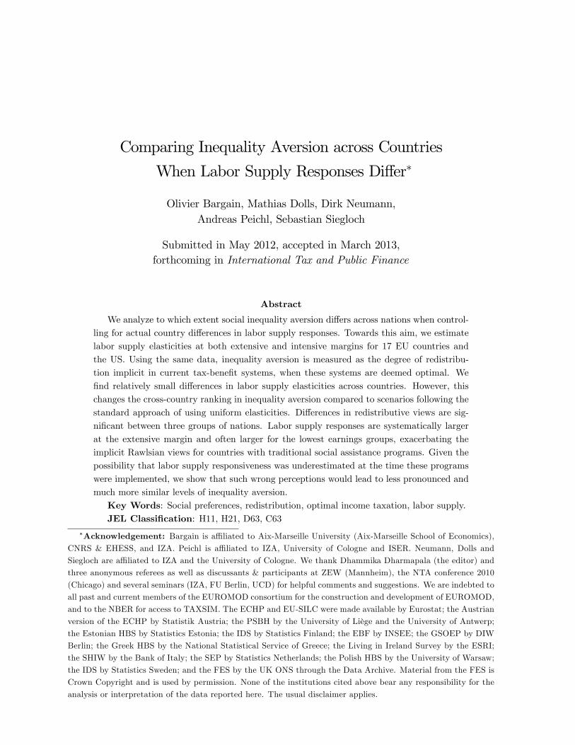
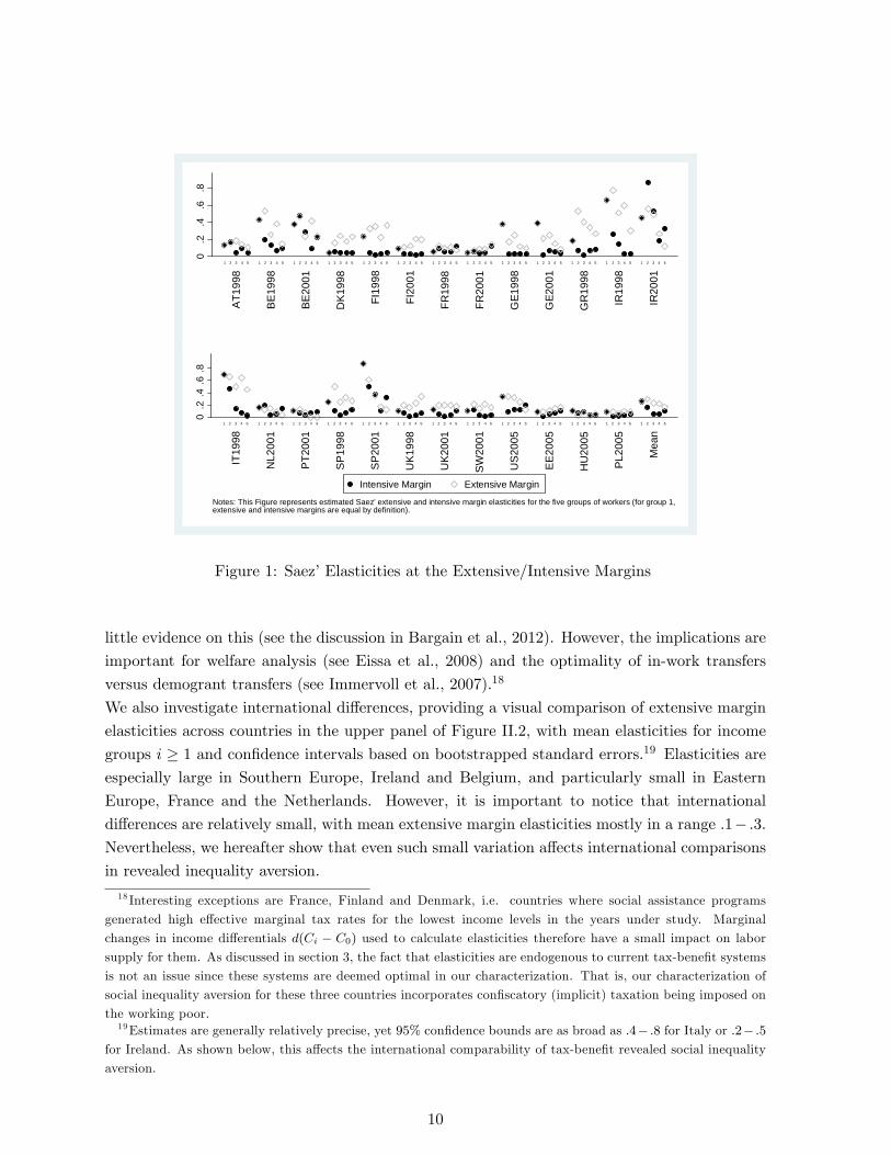
For a more convenient comparison across countries, point estimates are shown in Figure 1 below

for the di¤erent income groups. The �rst result is that responses at the extensive margin are

systematically larger than at the intensive margin (except for group 1, for which both margins

are identical by de�nition). This �nding generalizes previous results for the US (e.g. Eissa and

Liebman, 1996), Germany and the UK (Blundell et al., 2009).

A second result is that responses are usually larger for the lowest income groups of workers

(groups 1 and 2). Despite this being expected for single individuals, there is currently very17We calibrate uniform changes in disposable income at the individual level to obtain percent changes in income

gaps, as de�ned in (2) and (3). Total responses, measured as a change in the population shares in each income

group, are then obtained by aggregation to calculate �i and �i for i = 1; :::; I (see also Blundell et al., 2009).

9

0.2

.4.6

.8

AT1

998

BE

1998

BE

2001

DK

1998

FI19

98

FI20

01

FR19

98

FR20

01

GE1

998

GE2

001

GR

1998

IR19

98

IR20

01

1 2 3 4 5 1 2 3 4 5 1 2 3 4 5 1 2 3 4 5 1 2 3 4 5 1 2 3 4 5 1 2 3 4 5 1 2 3 4 5 1 2 3 4 5 1 2 3 4 5 1 2 3 4 5 1 2 3 4 5 1 2 3 4 5

0.2

.4.6

.8

IT19

98

NL2

001

PT2

001

SP

1998

SP

2001

UK

1998

UK

2001

SW

2001

US

2005

EE

2005

HU

2005

PL2

005

Mea

n

1 2 3 4 5 1 2 3 4 5 1 2 3 4 5 1 2 3 4 5 1 2 3 4 5 1 2 3 4 5 1 2 3 4 5 1 2 3 4 5 1 2 3 4 5 1 2 3 4 5 1 2 3 4 5 1 2 3 4 5 1 2 3 4 5

Notes: This Figure represents estimated Saez' extensive and intensive margin elasticities for the five groups of workers (for group 1,extensive and intensive margins are equal by definition).

Intensive Margin Extensive Margin

Figure 1: Saez�Elasticities at the Extensive/Intensive Margins

little evidence on this (see the discussion in Bargain et al., 2012). However, the implications are

important for welfare analysis (see Eissa et al., 2008) and the optimality of in-work transfers

versus demogrant transfers (see Immervoll et al., 2007).18

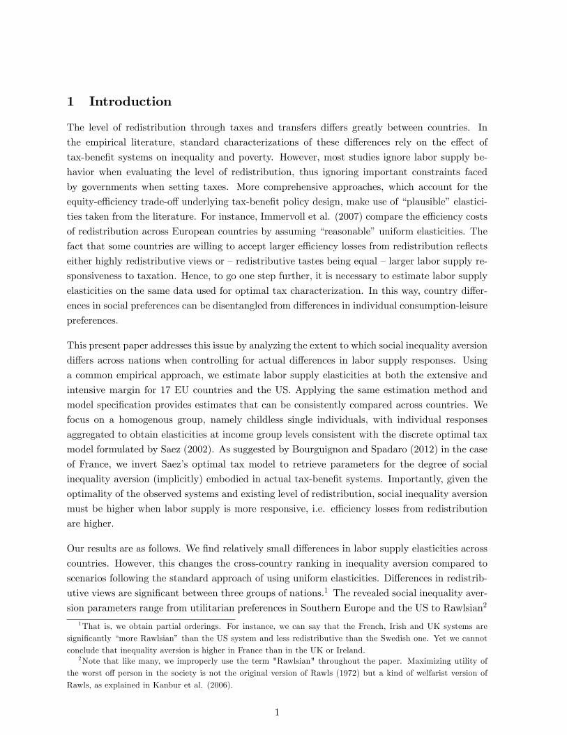
We also investigate international di¤erences, providing a visual comparison of extensive margin

elasticities across countries in the upper panel of Figure II.2, with mean elasticities for income

groups i � 1 and con�dence intervals based on bootstrapped standard errors.19 Elasticities areespecially large in Southern Europe, Ireland and Belgium, and particularly small in Eastern

Europe, France and the Netherlands. However, it is important to notice that international

di¤erences are relatively small, with mean extensive margin elasticities mostly in a range :1� :3.Nevertheless, we hereafter show that even such small variation a¤ects international comparisons

in revealed inequality aversion.

18 Interesting exceptions are France, Finland and Denmark, i.e. countries where social assistance programs

generated high e¤ective marginal tax rates for the lowest income levels in the years under study. Marginal

changes in income di¤erentials d(Ci � C0) used to calculate elasticities therefore have a small impact on laborsupply for them. As discussed in section 3, the fact that elasticities are endogenous to current tax-bene�t systems

is not an issue since these systems are deemed optimal in our characterization. That is, our characterization of

social inequality aversion for these three countries incorporates con�scatory (implicit) taxation being imposed on

the working poor.19Estimates are generally relatively precise, yet 95% con�dence bounds are as broad as :4� :8 for Italy or :2� :5

for Ireland. As shown below, this a¤ects the international comparability of tax-bene�t revealed social inequality

aversion.

10

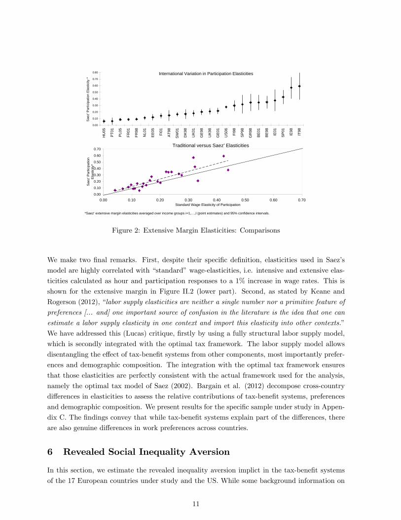
*Saez' extensive margin elasticities averaged over income groups i=1,… ,I (point estimates) and 95% confidence intervals.

Traditional versus Saez' Elasticities

0.00

0.10

0.20

0.30

0.40

0.50

0.60

0.70

0.00 0.10 0.20 0.30 0.40 0.50 0.60 0.70Standard Wage Elasticity of Participation

Sae

z' P

artic

ipat

ion

Ela

stic

ity*

International Variation in Participation Elasticities

0.00

0.10

0.20

0.30

0.40

0.50

0.60

0.70

0.80

HU

05

PT0

1

PL0

5

FR01

FR98

NL0

1

EE

05

FI01

AT9

8

SW

01

DK

98

UK

01

GE

98

UK

98

GE

01

US

06

FI98

SP

98

GR

98

BE

01

BE

98

IE01

SP

01

IE98

IT98

Sae

z' P

artic

ipat

ion 

Ela

stic

ity *

Figure 2: Extensive Margin Elasticities: Comparisons

We make two �nal remarks. First, despite their speci�c de�nition, elasticities used in Saez�s

model are highly correlated with �standard�wage-elasticities, i.e. intensive and extensive elas-

ticities calculated as hour and participation responses to a 1% increase in wage rates. This is

shown for the extensive margin in Figure II.2 (lower part). Second, as stated by Keane and

Rogerson (2012), �labor supply elasticities are neither a single number nor a primitive feature of

preferences [... and] one important source of confusion in the literature is the idea that one can

estimate a labor supply elasticity in one context and import this elasticity into other contexts.�

We have addressed this (Lucas) critique, �rstly by using a fully structural labor supply model,

which is secondly integrated with the optimal tax framework. The labor supply model allows

disentangling the e¤ect of tax-bene�t systems from other components, most importantly prefer-

ences and demographic composition. The integration with the optimal tax framework ensures

that those elasticities are perfectly consistent with the actual framework used for the analysis,

namely the optimal tax model of Saez (2002). Bargain et al. (2012) decompose cross-country

di¤erences in elasticities to assess the relative contributions of tax-bene�t systems, preferences

and demographic composition. We present results for the speci�c sample under study in Appen-

dix C. The �ndings convey that while tax-bene�t systems explain part of the di¤erences, there

are also genuine di¤erences in work preferences across countries.

6 Revealed Social Inequality Aversion

In this section, we estimate the revealed inequality aversion implict in the tax-bene�t systems

of the 17 European countries under study and the US. While some background information on

11

international di¤erences in tax-bene�t policies are summarized in Tables D.1-D.3 in Appendix

D, it is clear that the most important redistributive elements for single individuals are transfers

and progressive taxes, with the latter of particular importance in countries where singles are not

eligible for any income support (for instance, the US or Hungary).

6.1 Baseline results

We start our analysis by considering the e¤ective marginal tax rates (EMTRs) and e¤ective

participation tax rates (EPTRs), which provide an indication of the redistributive and incentive

e¤ects of the di¤erent welfare regimes. Appendix E highlights a U-shaped distribution of EMTRs

across income groups for most countries in Nordic and Continental Europe, which is well in line

with the results of Immervoll et al. (2007). This pattern is due to progressive taxation at the

top and means-tested social bene�ts at the bottom. Furthermore, the working poor (groups 1

and 2) have been rather excluded from redistribution for the years under consideration.20 In the

US and Southern Europe, the overall level of net taxation is usually lower and the distribution

of EMTRs generally �atter. There are exceptions, notably fairly high levels of e¤ective taxation

in upper income groups in Poland, Hungary, Ireland and Italy, as well as more pronounced

progressivity in Greece and Portugal.

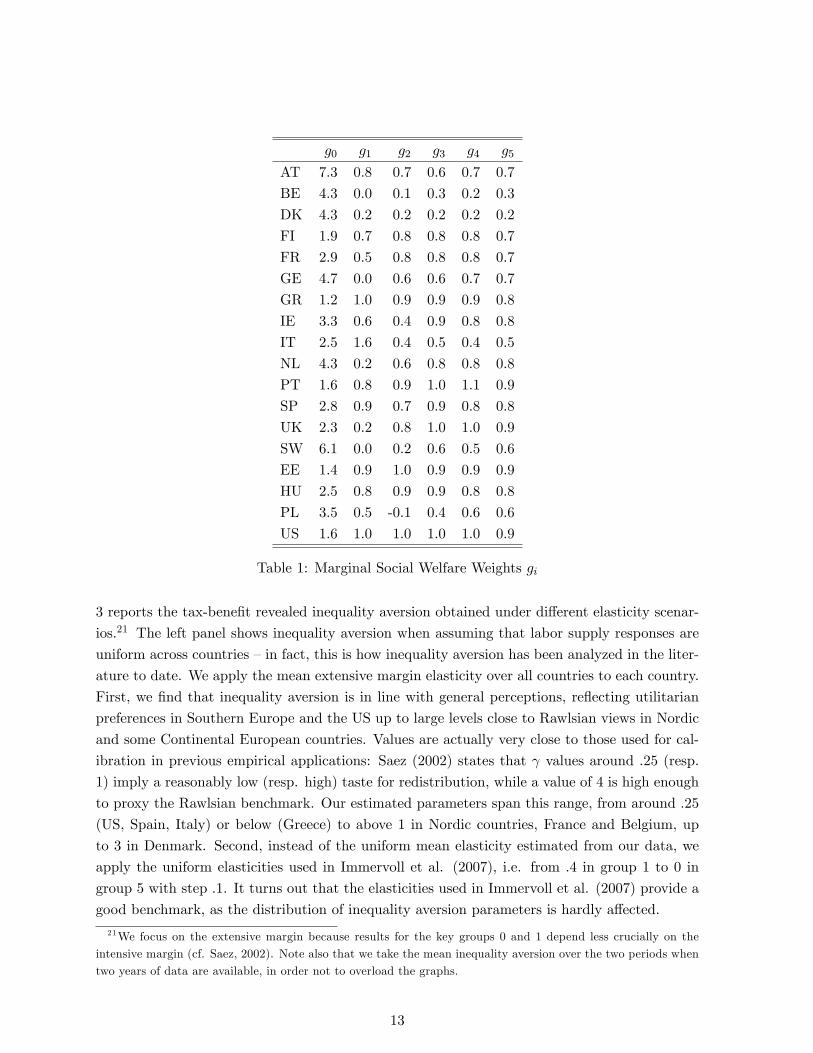
Next, we report and discuss the distribution of revealed marginal social welfare weights giunderlying our measure of inequality aversion, as derived from inverting the optimal tax formula

(see Table 1). A necessary condition for the implicit social welfare function to be Paretian, i.e.

non-decreasing at all productivity levels, is that weights gi are positive at all income levels.

Our results show that this is broadly the case for all countries and income groups. Marginal

social welfare weights for group 0 are much larger than for the rest of the population in Nordic

and Continental Europe, Ireland and the UK, which target non-marginal transfers towards the

bottom of the distribution. As found by considering EMTR, the welfare weights pattern is much

�atter in countries characterized by little redistribution through social transfers (Southern and

Eastern Europe, the US). However, for this group of countries smaller weights on top incomes

re�ect higher tax progressivity (Portugal and Greece), while uniformly low weights on non-poor

groups re�ect high tax levels (Italy). Weights on group 1 (and sometimes 2) are smallest in

countries with generous social assistance schemes, re�ecting distortions imposed on the working

poor as discussed in the EMTR analysis.

We estimate our main indicator of social inequality aversion, i.e. the single-value index of ,

according to equation (5) based on the dsitributions of marginal social welfare weights. Figure

20 International heterogeneity in the degree of redistribution is not a¤ected by the treatment of unemployment

bene�ts (UB), i.e. whether they are counted as part of the redistribution function or market income (according to

a pure insurance mechanism). Countries that do not redistribute much among childless single individuals do not

redistribute much in general (see Figure E.2. in Appendix E). This suggests that redistribution among this group

is representative of overall international di¤erences in tastes for vertical equity, con�rming that we can conduct

the analysis on single individuals.

12

g0 g1 g2 g3 g4 g5

AT 7.3 0.8 0.7 0.6 0.7 0.7

BE 4.3 0.0 0.1 0.3 0.2 0.3

DK 4.3 0.2 0.2 0.2 0.2 0.2

FI 1.9 0.7 0.8 0.8 0.8 0.7

FR 2.9 0.5 0.8 0.8 0.8 0.7

GE 4.7 0.0 0.6 0.6 0.7 0.7

GR 1.2 1.0 0.9 0.9 0.9 0.8

IE 3.3 0.6 0.4 0.9 0.8 0.8

IT 2.5 1.6 0.4 0.5 0.4 0.5

NL 4.3 0.2 0.6 0.8 0.8 0.8

PT 1.6 0.8 0.9 1.0 1.1 0.9

SP 2.8 0.9 0.7 0.9 0.8 0.8

UK 2.3 0.2 0.8 1.0 1.0 0.9

SW 6.1 0.0 0.2 0.6 0.5 0.6

EE 1.4 0.9 1.0 0.9 0.9 0.9

HU 2.5 0.8 0.9 0.9 0.8 0.8

PL 3.5 0.5 -0.1 0.4 0.6 0.6

US 1.6 1.0 1.0 1.0 1.0 0.9

Table 1: Marginal Social Welfare Weights gi

3 reports the tax-bene�t revealed inequality aversion obtained under di¤erent elasticity scenar-

ios.21 The left panel shows inequality aversion when assuming that labor supply responses are

uniform across countries �in fact, this is how inequality aversion has been analyzed in the liter-

ature to date. We apply the mean extensive margin elasticity over all countries to each country.

First, we �nd that inequality aversion is in line with general perceptions, re�ecting utilitarian

preferences in Southern Europe and the US up to large levels close to Rawlsian views in Nordic

and some Continental European countries. Values are actually very close to those used for cal-

ibration in previous empirical applications: Saez (2002) states that values around :25 (resp.

1) imply a reasonably low (resp. high) taste for redistribution, while a value of 4 is high enough

to proxy the Rawlsian benchmark. Our estimated parameters span this range, from around :25

(US, Spain, Italy) or below (Greece) to above 1 in Nordic countries, France and Belgium, up

to 3 in Denmark. Second, instead of the uniform mean elasticity estimated from our data, we

apply the uniform elasticities used in Immervoll et al. (2007), i.e. from :4 in group 1 to 0 in

group 5 with step :1. It turns out that the elasticities used in Immervoll et al. (2007) provide a

good benchmark, as the distribution of inequality aversion parameters is hardly a¤ected.

21We focus on the extensive margin because results for the key groups 0 and 1 depend less crucially on the

intensive margin (cf. Saez, 2002). Note also that we take the mean inequality aversion over the two periods when

two years of data are available, in order not to overload the graphs.

13

0 1 2 3Social inequality aversion

DK

SW

BE

FR

NL

FI

AT

UK

GE

HU

IE

PL

EE

PT

SP

US

IT

GR

Uniform elasticities: compare with Immervoll et al.

elast. of Immervoll & al. mean estimated elast.note: countries ranked according to the 2nd measure (using mean elast.)

0 1 2 3Social inequality aversion

BE

DK

SW

NL

FI

IE

FR

AT

GE

UK

PL

HU

SP

IT

EE

PT

US

GR

Ranking affected when using specific elast.

mean estimated elast. country­specific elast.note: countries ranked according to the second measure (our baseline)

0 1 2 3Social inequality aversion

BE

SW

DK

NL

FI

FR

GE

IE

UK

AT

PL

HU

SP

IT

US

EE

PT

GR

Pairwise comparisons not always significant

lower bound elast. upper bound elast.note: countries ranked according to lower bound

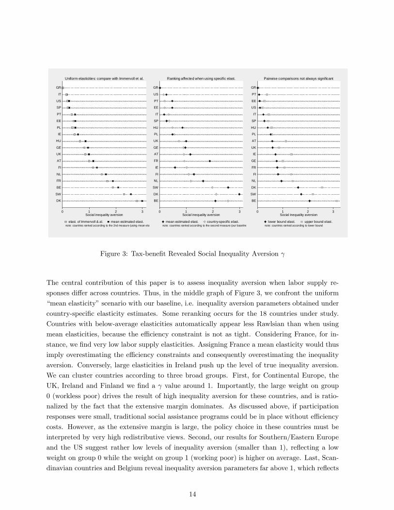
Figure 3: Tax-bene�t Revealed Social Inequality Aversion

The central contribution of this paper is to assess inequality aversion when labor supply re-

sponses di¤er across countries. Thus, in the middle graph of Figure 3, we confront the uniform

�mean elasticity�scenario with our baseline, i.e. inequality aversion parameters obtained under

country-speci�c elasticity estimates. Some reranking occurs for the 18 countries under study.

Countries with below-average elasticities automatically appear less Rawlsian than when using

mean elasticities, because the e¢ ciency constraint is not as tight. Considering France, for in-

stance, we �nd very low labor supply elasticities. Assigning France a mean elasticity would thus

imply overestimating the e¢ ciency constraints and consequently overestimating the inequality

aversion. Conversely, large elasticities in Ireland push up the level of true inequality aversion.

We can cluster countries according to three broad groups. First, for Continental Europe, the

UK, Ireland and Finland we �nd a value around 1. Importantly, the large weight on group

0 (workless poor) drives the result of high inequality aversion for these countries, and is ratio-

nalized by the fact that the extensive margin dominates. As discussed above, if participation

responses were small, traditional social assistance programs could be in place without e¢ ciency

costs. However, as the extensive margin is large, the policy choice in these countries must be

interpreted by very high redistributive views. Second, our results for Southern/Eastern Europe

and the US suggest rather low levels of inequality aversion (smaller than 1), re�ecting a low

weight on group 0 while the weight on group 1 (working poor) is higher on average. Last, Scan-

dinavian countries and Belgium reveal inequality aversion parameters far above 1, which re�ects

14

an even higher weight on group 0 than observed for the �rst group of countries (see Table 1).

Finally, we provide 95% con�dence bands for the inequality aversion parameter, accounting for

the standard errors of the estimated participation elasticities (see the right panel of Figure 3).

Some comparisons are unambiguous (e.g. redistributive views in Sweden are more Rawlsian

than in the US). However, di¤erences are not signi�cant for all pairs of countries, i.e. the or-

dering of countries�redistributive tastes is incomplete (for instance, di¤erences between Sweden

and Denmark). However, reassuringly, we can distinguish the same three groups of countries as

delineated above.

6.2 Sensitivity Analyses

Our baseline results characterize the redistributive preferences embodied in actual tax-bene�t

systems given estimated elasticities and reasonable income group de�nitions. Despite it being

plausible to assume that observed tax-bene�t systems are optimal for the governments who

implemented them, they may have actually had completely di¤erent priors about these two key

parameters of the model.

Elasticities. We �rst discuss what would happen if we use �wrong�labor supply elastici-

ties. In fact, it is possible that potential labor supply responses were underestimated or ignored

by policymakers in continental Europe when generous demogrant policies were designed and

implemented. It was only in the late 1990s that numerous policy reports released in Europe

highlighted the possibility that safety nets designed to prevent extreme poverty caused work

disincentives and �inactivity traps�. The same concern that welfare programs had pushed part

of the population into a state of welfare dependency had previously led to the 1996 welfare

reform in the US (see Piketty and Saez, 2013).22

Therefore, we suggest a polar case where extensive margin responses are set to zero, i.e. �sim-

ulating� the case that politicians completely ignored behavioral responses. The left panel of

Figure 4 shows that the international ranking is broadly preserved. However, absolute inequal-

ity aversion mechanically decreases: preferences are less Rawlsian if participation responses, i.e.

mobility between the workless poor and the working poor, are ignored. Consequently, most of

the di¤erences between countries vanish. However, Belgium, Sweden, Denmark, and to some

22 In the context of the US and the UK, Piketty and Saez (2013) argue that governments retargeted transfers

from groups unable to work to bene�ciaries who were potentially able to work. This trend has led to a shift from

traditional means-tested social assistance programs toward in-work bene�ts. This policy adjustment to the moral

hazard problem attached to traditional demogrant policies can be seen as a revision of beliefs about labor supply

responses and/or a change in social preferences (social welfare weights on non-workers fall relative to those on low

income workers, as society believes that a majority of the former can actually work). It is probably impossible

to di¤erentiate between these two aspects (i.e. it is equivalent to say that the society reassesses labor supply

responses upwards or increasingly favors desert-sensitive policies). As discussed in section 2, we do not attempt

to explain how social preferences are formed and why they change �yet it is interesting to underscore the political

economy forces at play and the possible role of international in�uence, with some noticeable convergence across

countries on the principle of �making work pay�(see Banks et al., 2005).

15

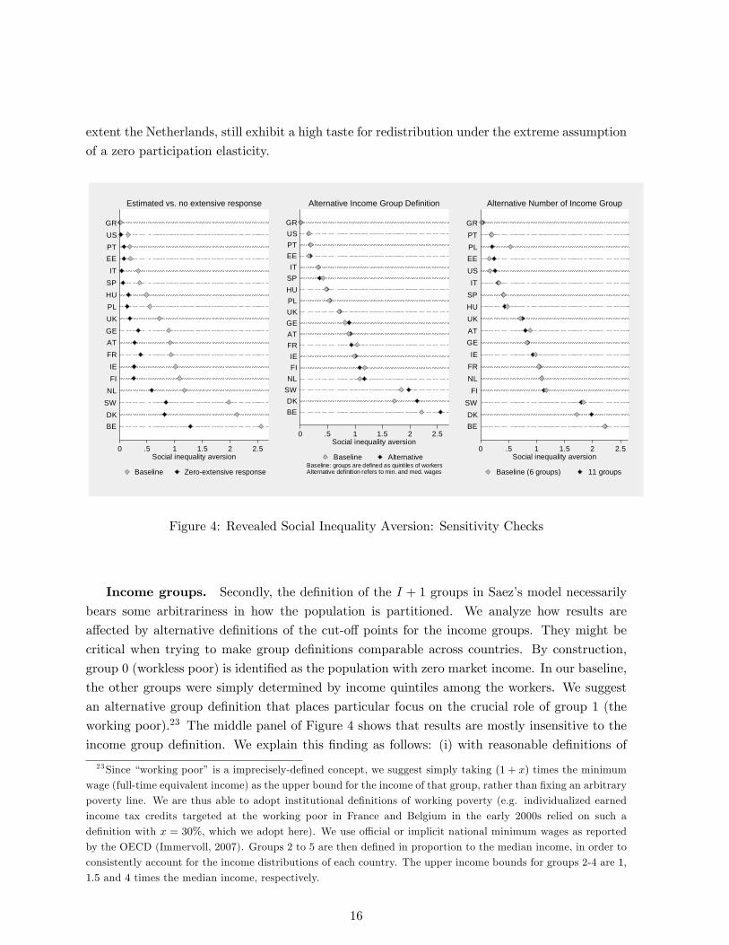
extent the Netherlands, still exhibit a high taste for redistribution under the extreme assumption

of a zero participation elasticity.

0 .5 1 1.5 2 2.5Social inequality aversion

BEDK

SWNLFIIE

FRATGEUKPLHUSPIT

EEPTUSGR

Estimated vs. no extensive response

Baseline Zero­extensive response

0 .5 1 1.5 2 2.5Social inequality aversion

BEDK

SWNLFIIE

FRATGEUKPLHUSPIT

EEPTUSGR

Alternative Income Group Definition

Baseline AlternativeBaseline: groups are defined as quintiles of workersAlternative definition refers to min. and med. wages

0 .5 1 1.5 2 2.5Social inequality aversion

BEDK

SWFI

NLFRIE

GEATUKHUSPIT

USEEPLPTGR

Alternative Number of Income Group

Baseline (6 groups) 11 groups

Figure 4: Revealed Social Inequality Aversion: Sensitivity Checks

Income groups. Secondly, the de�nition of the I + 1 groups in Saez�s model necessarily

bears some arbitrariness in how the population is partitioned. We analyze how results are

a¤ected by alternative de�nitions of the cut-o¤ points for the income groups. They might be

critical when trying to make group de�nitions comparable across countries. By construction,

group 0 (workless poor) is identi�ed as the population with zero market income. In our baseline,

the other groups were simply determined by income quintiles among the workers. We suggest

an alternative group de�nition that places particular focus on the crucial role of group 1 (the

working poor).23 The middle panel of Figure 4 shows that results are mostly insensitive to the

income group de�nition. We explain this �nding as follows: (i) with reasonable de�nitions of

23Since �working poor� is a imprecisely-de�ned concept, we suggest simply taking (1 + x) times the minimum

wage (full-time equivalent income) as the upper bound for the income of that group, rather than �xing an arbitrary

poverty line. We are thus able to adopt institutional de�nitions of working poverty (e.g. individualized earned

income tax credits targeted at the working poor in France and Belgium in the early 2000s relied on such a

de�nition with x = 30%, which we adopt here). We use o¢ cial or implicit national minimum wages as reported

by the OECD (Immervoll, 2007). Groups 2 to 5 are then de�ned in proportion to the median income, in order to

consistently account for the income distributions of each country. The upper income bounds for groups 2-4 are 1,

1:5 and 4 times the median income, respectively.

16

group 1, we always capture the income gap between groups 0, 1 and 2 to some extent; (ii) the

rest of the social welfare weight distribution is relatively �at, so alternative de�nitions of higher

income groups have little impact.

Finally, we provide a sensitivity analysis with regard to the number of income groups. To

ease comparisons across countries, we have initially opted for a small number of income groups

(I + 1 = 6), checking results obtained with I = 11 groups (10 groups of workers and the

unemployed). The right panel of Figure 4 shows very few changes compared to the baseline.

7 Conclusion

This paper retrieves social inequality aversion parameters consistent with current tax-bene�t

systems in 18 Western countries under the assumption of optimality, while controlling for di¤er-

ences in labor supply responsiveness. Labor supply elasticities have been estimated on the same

data used for the optimal tax inversion. We �nd relatively small di¤erences in labor supply

elasticities across countries, yet resulting redistributive views are signi�cantly di¤erent between

three groups of nations. Social inequality aversion is highest in Nordic and some Continental

European countries, pointing to Rawlsian preferences, while Southern Europe and the US re�ect

a very low inequality aversion close to utilitarian views. Furthermore, countries with Rawlsian

preferences only appear so because responses at the extensive margin �the dominant margin �

are taken into account. If we impose zero labor supply responses, re�ecting the possibility that

policymakers ignored e¢ ciency constraints at the time traditional social transfers were put in

place, revealed redistributive tastes become less pronounced and much more similar. This high-

lights the importance of accounting for e¢ ciency constraints when assessing social inequality

aversion.

Future research should extend the scope of the policies under consideration. Indeed, we have

considered a partial optimization problem by looking at direct taxes and transfers. Some other

policies may well have redistributive e¤ects, including non-cash bene�ts and public goods. An-

other limit to our work is the assumption of only one type of behavioral response, namely labor

supply. This appears acceptable as a �rst approximation, especially as we focus on workers

(thus excluding capitalists). Despite estimates being di¢ cult to obtain, more general analyses

could explore elasticities of other margins, e.g. migration, tax evasion or long-run behavioral

responses such as educational and career choices. In addition, it might be worthwhile to extent

the political economy perspective by accounting for the political process that generated the

observed tax bene�t systems in the analysis. For instance, political economy forces could be

modelled as distortions in the optimal tax design before the inversion procedure is applied.

17

References

[1] Acemoglu, D., M. Golosov and A. Tsyvinski (2010): "Dynamic Mirrlees taxation under

political economy constraints", Review of Economic Studies, 77 (3), 841�881.

[2] Ackert, L.F., J. Martinez-Vazquez and M. Rider (2007): "Social preferences and tax policy

design: some experimental evidence", Economic Inquiry, 45 (3), 487�501.

[3] Ahmad, E. and N. Stern (1984): "The theory of reform and Indian indirect taxes", Journal

of Public Economics, 25, 259-298.

[4] Alesina, A. and P. Giuliano (2011): "Preferences for Redistribution" in J. Benhabib, M.O.

Jackson and A. Bisin, Handbook of Social Economics, 1B, Amsterdam: Elsevier, 93-132.

[5] Amiel, Y., J. Creedy, and S. Hurn (1999): "Measuring attitudes towards inequality", Scan-

dinavian Journal of Economics, 101, 83-96.

[6] Banks, J., R. Disney, A. Duncan and J. Van Reenen (2005): "The Internationalisation of

Public Welfare Policy", Economic Journal, 115, C62-C8.

[7] Bargain, O. and A. Spadaro (2008): "Optimal taxation, social contract and the four worlds

of welfare capitalism", UCD School Of Economics, Working Papers No. 200816.

[8] Bargain, O., K. Orsini and A. Peichl (2012): "Comparing Labor Supply Elasticities in

Europe and the US: New Results", IZA Discussion Paper 6735.

[9] Blundell, R. and T. MaCurdy (1999): "Labor Supply: A Review of Alternative Ap-

proaches", in O. Ashenfelter and D. Card (eds.), Handbook of Labor Economics, 3A,

Amsterdam: Elsevier, 1559-1695.

[10] Blundell, R.W., A. Duncan, J. McCrae and C. Meghir (2000): "The Labour Market Impact

of the Working Families�Tax Credit", Fiscal Studies, 21, 1, 75-103.

[11] Blundell, R., M. Brewer, P. Haan and A. Shephard (2009): "Optimal income taxation of

lone mothers: an empirical comparison of the UK and Germany", Economic Journal,

119 (535), F101-F121.

[12] Bourguignon, F. and A. Spadaro (2012): "Tax-bene�t revealed social preferences", Journal

of Economic Inequality, 10(1), 75-108.

[13] Castanheira, M., G. Nicodème and P. Profeta (2012): "On the political economics of tax

reforms: survey and empirical assessment", International Tax and Public Finance,19,

598�624.

[14] Christiansen, V. and E.S. Jansen (1978): "Implicit Social Preferences in the Norwegian

System of Indirect Taxation", Journal of Public Economics, 10 , 217-245.

[15] Coughlin, P.J. (1992), Probabilistic Voting Theory, Cambridge University Press.

[16] Corneo, G. and H.P. Grüner (2002): "Individual preferences for political redistribution",

Journal of Public Economics, 83(1), 83-107.

18

[17] Decoster, A. and E. Schokkaert (1989): "Equity and e¢ ciency of a reform of Belgian indirect

taxes", Recherches Economiques de Louvain, 55(2), 155-176.

[18] Diamond, P. (1980): "Income taxation with �xed hours of work", Journal of Public Eco-

nomics, 13(1), 101-110.

[19] Duclos, J.-Y. (2000): "Gini Indices and the Redistribution of Income", International Tax

and Public Finance, 7, 141-162.

[20] Eissa, N. and J.B. Liebman (1996): "Labor supply response to the earned income tax

credit", Quarterly Journal of Economics, 111(2), 605�37.

[21] Eissa, N. and H. Hoynes (2011): "Redistribution and Tax Expenditures: The Earned In-

come Tax Credit", National Tax Journal, 64 (2, Part 2), 689�730.

[22] Eissa, N., H. J. Kleven and C.T. Kreiner (2008): "Evaluation of Four Tax Reforms in the

United States: Labor Supply and Welfare E¤ects for Single Mothers", Journal of Public

Economics, 92, 795�816.

[23] Feenberg, D. and E. Coutts (1993): "An introduction to the TAXSIM model", Journal of

Policy Analysis and Management, 12 (1), 189�194.

[24] Fehr E. and K.M. Schmidt (1999): "A theory of fairness, competition and cooperation",

Quarterly Journal of Economics, 114, 817-868.

[25] Fleurbaey, M. (2008), Fairness, responsibility and welfare. Oxford University Press, Oxford.

[26] Fong, C. (2001): "Social Preferences, Self-interest, and the Demand for Redistribution",

Journal of Public Economics, 82(2), 225-246.

[27] Gordon, R.H. and J.B. Cullen (2011): "Income Redistribution in a Federal System of

Governments", Journal of Public Economics, forthcoming.

[28] Hoynes, H. W. (1996): �Welfare transfers in two-parent families: Labor supply and welfare

participation under AFDC-UP�, Econometrica, 64(29), 295-332.

[29] Immervoll H., H. J. Kleven, C.T. Kreiner and E. Saez (2007): "Welfare reform in European

countries: A microsimulation analysis", Economic Journal, 117(516), 1-44.

[30] Isaksson, A.-S. and A. Lindskog (2009): "Preferences for redistribution: A country com-

parison of fairness judgements", Journal of Economic Behavior and Organization 72(3),

884�902.

[31] Kanbur, R. and M. Tuomala (2011): "Charitable Conservatism, Poverty Radicalism and

Inequality Aversion", Journal of Economic Inequality, Vol. 9(3), 417-431.

[32] Kanbur, R., J. Pirttilä and M. Tuomala (2006): "Non-welfarist optimal taxation and be-

havioural public economics", Journal of Economic Surveys, 20(5), 849-868.

[33] Keane, M. and R. Rogerson (2012): "Reconciling Micro and Macro Labor Supply Elastici-

ties: A Structural Perspective", Journal of Economic Literature, 50(2), 464-476.

19

[34] Lambert P..J., Millimet D.L. and Slottje D. (2003) �Inequality aversion and the natural rate

of subjective inequality�, Journal of Public Economics, 87(5): 1061-1090(30).

[35] Madden, D. (1996): "An analysis of indirect tax reform in Ireland in the 1980s", Fiscal

Studies, 16: 18-37.

[36] Piketty, T. (1995): �Social Mobility and Redistributive Politics,� Quarterly Journal of

Economics, 110(3), 551-584.

[37] Piketty, T. and E. Saez (2013): �Optimal Labor Income Taxation�, Handbook of Public

Economics, Vol. 5, (Amsterdam: North Holland), forthcoming.

[38] Ross T.W. (1984): "Uncovering Regulator�s Social Welfare Weights", Rand Journal of

Economics 15, 152�155.

[39] Saez, E. (2002): "Optimal income transfer programs: Intensive versus extensive labor sup-

ply responses", Quarterly Journal of Economics, 117(3), 1039-1073.

[40] Saez, E. and S. Stantcheva (2012): "Endogenous Social Welfare Weights for Optimal Tax

Theory", mimeo.

[41] Singhal, M. (2008): "Quantifying preferences for redistribution", paper presented at the

AEA Annual Meeting January 2009.

[42] Spadaro A. (2008): "Optimal taxation, social contract and the four worlds of welfare capi-

talism". PSE Working Paper no 38-2008.

[43] Stern, N. (1977): "Welfare Weights and the Elasticity of the Marginal Valuation of Income",

in M. Artis and R. Nobay, eds., Studies in Modern Economic Analysis, (Oxford: Basil

Blackwell Publishers).

[44] Sutherland, H. (2001): "Final report EUROMOD: an integrated European bene�t-tax

model", EUROMOD Working Paper No. EM9/01, ISER.

[45] van Soest, A. (1995): "Structural models of family labor supply: a discrete choice ap-

proach", Journal of Human Resources, 30(1), 63-88.

20

I Descriptive Statistics

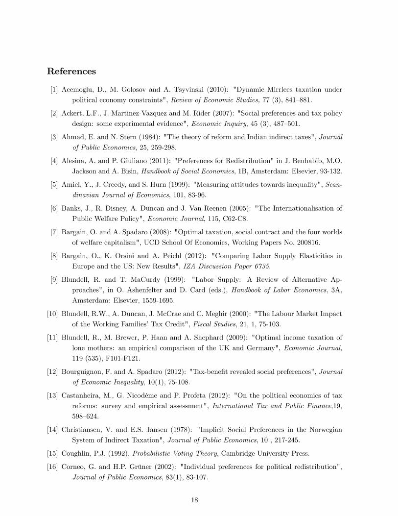
Since the selected population is relatively homogenous, Tables I.1 and I.2 essentially focus on

the characteristics of the discretized income groups, i.e., the main ingredients of the optimal tax

model. This includes income group shares hi, average levels of gross income Yi and disposable

income Ci for each group i = 0; :::5 .We also report e¤ective �marginal�tax rates T 0i =Ti�Ti�1Yi�Yi�1

and e¤ective participation tax rates Ti�T0Yi�Y0 .

21

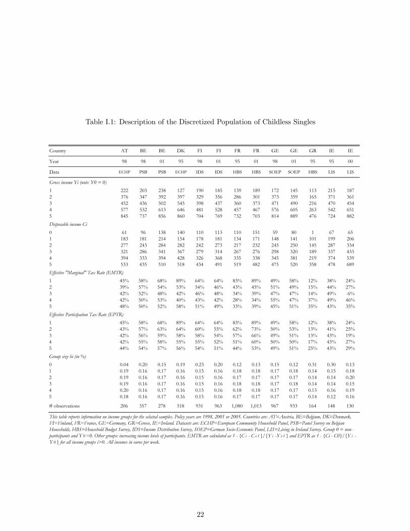
Table I.1: Description of the Discretized Population of Childless Singles

Country AT BE BE DK FI FI FR FR GE GE GR IE IE

Year 98 98 01 95 98 01 95 01 98 01 95 95 00

Data ECHP PSB PSB ECHP IDS IDS HBS HBS SOEP SOEP HBS LIS LIS

Gross income Yi (note: Y0 = 0)1 222 203 238 127 190 185 139 189 172 145 113 215 1872 376 347 392 397 329 356 286 301 373 359 165 371 3613 452 436 502 545 398 437 360 373 471 490 216 470 4544 577 532 613 646 481 528 457 467 576 605 263 542 6515 845 737 856 860 704 769 732 703 814 889 476 724 882Disposable income Ci0 61 96 138 140 110 113 110 151 59 80 1 67 651 183 181 214 154 178 181 134 171 148 141 101 199 2062 277 243 284 282 242 273 217 232 245 250 145 287 3343 321 286 341 367 279 314 267 276 298 320 189 337 4334 394 333 394 428 326 368 335 338 345 381 219 374 5395 533 435 510 518 434 491 519 482 475 520 358 478 689Effective "Marginal" Tax Rate (EMTR)1 45% 58% 68% 89% 64% 64% 83% 89% 49% 58% 12% 38% 24%2 39% 57% 54% 53% 54% 46% 43% 45% 51% 49% 15% 44% 27%3 42% 52% 48% 42% 46% 48% 34% 39% 47% 47% 14% 49% ­6%4 42% 50% 53% 40% 43% 42% 28% 34% 55% 47% 37% 49% 46%5 48% 50% 52% 58% 51% 49% 33% 39% 45% 51% 35% 43% 35%Effective Participation Tax Rate (EPTR)1 45% 58% 68% 89% 64% 64% 83% 89% 49% 58% 12% 38% 24%2 43% 57% 63% 64% 60% 55% 62% 73% 50% 53% 13% 41% 25%3 42% 56% 59% 58% 58% 54% 57% 66% 49% 51% 13% 43% 19%4 42% 55% 58% 55% 55% 52% 51% 60% 50% 50% 17% 43% 27%5 44% 54% 57% 56% 54% 51% 44% 53% 49% 51% 25% 43% 29%Group size hi (in %)0 0.04 0.20 0.15 0.19 0.23 0.20 0.12 0.13 0.15 0.12 0.31 0.30 0.131 0.19 0.16 0.17 0.16 0.15 0.16 0.18 0.18 0.17 0.18 0.14 0.15 0.182 0.19 0.16 0.17 0.16 0.15 0.16 0.17 0.17 0.17 0.17 0.14 0.14 0.203 0.19 0.16 0.17 0.16 0.15 0.16 0.18 0.18 0.17 0.18 0.14 0.14 0.154 0.20 0.16 0.17 0.16 0.15 0.16 0.18 0.18 0.17 0.17 0.13 0.16 0.195 0.18 0.16 0.17 0.16 0.15 0.16 0.17 0.17 0.17 0.17 0.14 0.12 0.16

# observations 206 357 278 518 931 963 1,080 1,013 967 933 164 148 130

This table reports information on income groups for the selected samples. Policy years are 1998, 2001 or 2005. Countries are: AT=Austria, BE=Belgium, DK=Denmark,FI=Finland, FR=France, GE=Germany, GR=Greece, IE=Ireland. Datasets are: ECHP=European Community Household Panel, PSB=Panel Survey on BelgianHouseholds, HBS=Household Budget Survey, IDS=Income Distribution Survey, SOEP=German Socio­Economic Panel, LIS=Living in Ireland Survey. Group 0 = non­participants and Y 0 =0. Other groups: increasing income levels of participants. EMTR are calculated as 1 ­ {C i ­ C i­1 }/{Y i  ­Y i­1 } and EPTR as 1 ­ {Ci ­ C0}/{Y i  ­Y 0 } for all income groups i>0. All incomes in euros per week.

22

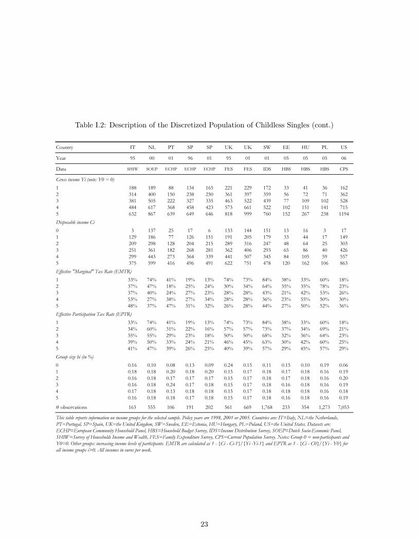
Table I.2: Description of the Discretized Population of Childless Singles (cont.)

Country IT NL PT SP SP UK UK SW EE HU PL US

Year 95 00 01 96 01 95 01 01 05 05 05 06

Data SHIW SOEP ECHP ECHP ECHP FES FES IDS HBS HBS HBS CPS

Gross income Yi (note: Y0 = 0)1 188 189 88 134 165 221 229 172 33 41 36 1622 314 400 150 238 250 361 397 359 56 72 71 3623 381 505 222 327 335 463 522 439 77 109 102 5284 484 617 368 458 423 573 661 522 102 151 141 7155 632 867 639 649 646 818 999 760 152 267 238 1194Disposable income Ci0 3 137 25 17 6 133 144 151 13 16 3 171 129 186 77 126 151 191 205 179 33 44 17 1492 209 298 128 204 215 289 316 247 48 64 25 3033 251 361 182 268 281 362 406 293 65 86 40 4264 299 443 273 364 339 441 507 345 84 105 59 5575 375 599 416 496 491 622 751 478 120 162 106 863Effective "Marginal" Tax Rate (EMTR)1 33% 74% 41% 19% 13% 74% 73% 84% 38% 33% 60% 18%2 37% 47% 18% 25% 24% 30% 34% 64% 35% 35% 78% 23%3 37% 40% 24% 27% 23% 28% 28% 43% 21% 42% 53% 26%4 53% 27% 38% 27% 34% 28% 28% 36% 23% 55% 50% 30%5 48% 37% 47% 31% 32% 26% 28% 44% 27% 50% 52% 36%Effective Participation Tax Rate (EPTR)1 33% 74% 41% 19% 13% 74% 73% 84% 38% 33% 60% 18%2 34% 60% 31% 22% 16% 57% 57% 73% 37% 34% 69% 21%3 35% 55% 29% 23% 18% 50% 50% 68% 32% 36% 64% 23%4 39% 50% 33% 24% 21% 46% 45% 63% 30% 42% 60% 25%5 41% 47% 39% 26% 25% 40% 39% 57% 29% 45% 57% 29%Group size hi (in %)0 0.16 0.10 0.08 0.13 0.09 0.24 0.15 0.11 0.15 0.10 0.19 0.061 0.18 0.18 0.20 0.18 0.20 0.15 0.17 0.18 0.17 0.18 0.16 0.192 0.16 0.18 0.17 0.17 0.17 0.15 0.17 0.18 0.17 0.18 0.16 0.203 0.16 0.18 0.24 0.17 0.18 0.15 0.17 0.18 0.16 0.18 0.16 0.194 0.17 0.18 0.13 0.18 0.18 0.15 0.17 0.18 0.18 0.18 0.16 0.185 0.16 0.18 0.18 0.17 0.18 0.15 0.17 0.18 0.16 0.18 0.16 0.19

# observations 163 555 106 191 202 561 669 1,768 233 354 1,273 7,053

This table reports information on income groups for the selected sample. Policy years are 1998, 2001 or 2005. Countries are: IT=Italy, NL=the Netherlands,PT=Portugal, SP=Spain, UK=the United Kingdom, SW=Sweden, EE=Estonia, HU=Hungary, PL=Poland, US=the United States. Datasets are:ECHP=European Community Household Panel, HBS=Household Budget Survey, IDS=Income Distribution Survey, SOEP=Dutch Socio­Economic Panel,SHIW=Survey of Households Income and Wealth, FES=Family Expenditure Survey, CPS=Current Population Survey. Notes: Group 0 = non­participants andY0=0. Other groups: increasing income levels of participants. EMTR are calculated as 1 ­ {Ci ­ Ci­1}/{Yi ­Yi­1} and EPTR as 1 ­ {Ci ­ C0}/{Yi ­ Y0} forall income groups i>0. All incomes in euros per week.

23

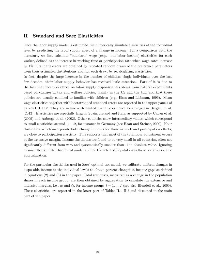
II Standard and Saez Elasticities

Once the labor supply model is estimated, we numerically simulate elasticities at the individual

level by predicting the labor supply e¤ect of a change in income. For a comparison with the

literature, we �rst calculate "standard" wage (resp. non-labor income) elasticities for each

worker, de�ned as the increase in working time or participation rate when wage rates increase

by 1%. Standard errors are obtained by repeated random draws of the preference parameters

from their estimated distributions and, for each draw, by recalculating elasticities.

In fact, despite the large increase in the number of childless single individuals over the last

few decades, their labor supply behavior has received little attention. Part of it is due to

the fact that recent evidence on labor supply responsiveness stems from natural experiments

based on changes in tax and welfare policies, mainly in the US and the UK, and that these

policies are usually con�ned to families with children (e.g., Eissa and Liebman, 1996). Mean

wage elasticities together with bootstrapped standard errors are reported in the upper panels of

Tables II.1�II.2. They are in line with limited available evidence as surveyed in Bargain et al.

(2012). Elasticities are especially large in Spain, Ireland and Italy, as supported by Callan et al.

(2009) and Aaberge et al. (2002). Other countries show intermediary values, which correspond

to small elasticities around :1 �:2, for instance in Germany (see Haan and Steiner, 2000). Hour

elasticities, which incorporate both change in hours for those in work and participation e¤ects,

are close to participation elasticity. This supports that most of the total hour adjustment occurs

at the extensive margin. Income elasticities are found to be very small in all countries, often not

signi�cantly di¤erent from zero and systematically smaller than :1 in absolute value. Ignoring

income e¤ects in the theoretical model and for the selected population is therefore a reasonable

approximation.

For the particular elasticities used in Saez�optimal tax model, we calibrate uniform changes in

disposable income at the individual levels to obtain percent changes in income gaps as de�ned

in equations (2) and (3) in the paper. Total responses, measured as a change in the population

shares in each income group, are then obtained by aggregation to calculate the extensive and

intensive margins, i.e., �i and �i; for income groups i = 1; :::; I (see also Blundell et al., 2009).

These elasticities are reported in the lower part of Tables II.1�II.2 and discussed in the main

part of the paper.

24

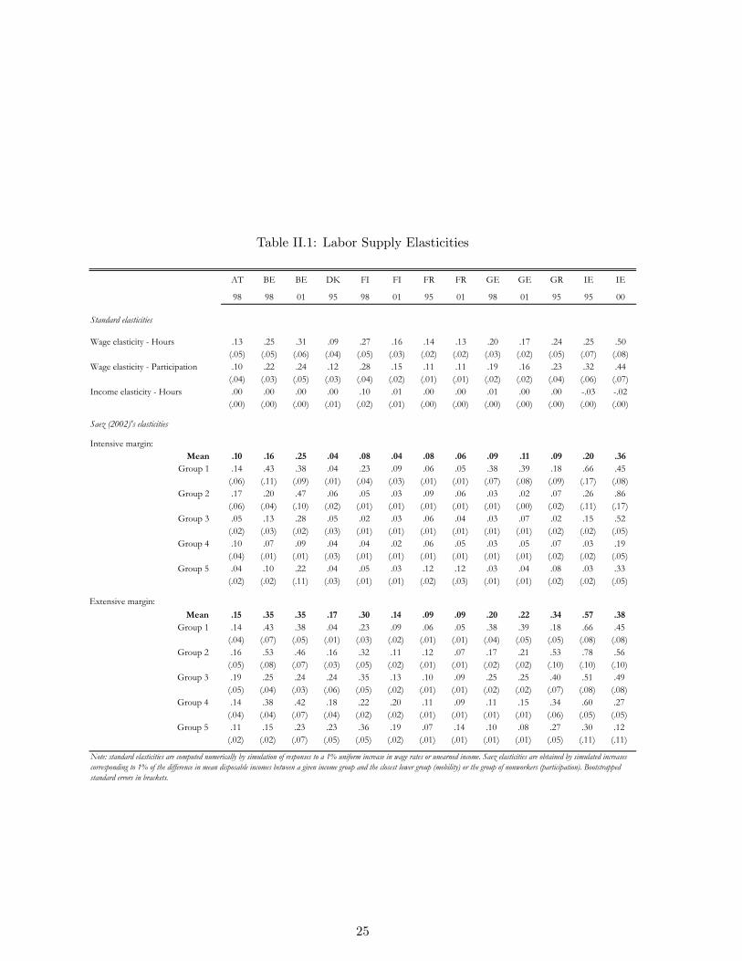
Table II.1: Labor Supply Elasticities

AT BE BE DK FI FI FR FR GE GE GR IE IE

98 98 01 95 98 01 95 01 98 01 95 95 00

Standard elasticities

Wage elasticity ­ Hours .13 .25 .31 .09 .27 .16 .14 .13 .20 .17 .24 .25 .50(.05) (.05) (.06) (.04) (.05) (.03) (.02) (.02) (.03) (.02) (.05) (.07) (.08)

Wage elasticity ­ Participation .10 .22 .24 .12 .28 .15 .11 .11 .19 .16 .23 .32 .44(.04) (.03) (.05) (.03) (.04) (.02) (.01) (.01) (.02) (.02) (.04) (.06) (.07)

Income elasticity ­ Hours .00 .00 .00 .00 .10 .01 .00 .00 .01 .00 .00 ­.03 ­.02(.00) (.00) (.00) (.01) (.02) (.01) (.00) (.00) (.00) (.00) (.00) (.00) (.00)

Saez (2002)'s elasticities

Intensive margin:Mean .10 .16 .25 .04 .08 .04 .08 .06 .09 .11 .09 .20 .36

Group 1 .14 .43 .38 .04 .23 .09 .06 .05 .38 .39 .18 .66 .45(.06) (.11) (.09) (.01) (.04) (.03) (.01) (.01) (.07) (.08) (.09) (.17) (.08)

Group 2 .17 .20 .47 .06 .05 .03 .09 .06 .03 .02 .07 .26 .86(.06) (.04) (.10) (.02) (.01) (.01) (.01) (.01) (.01) (.00) (.02) (.11) (.17)

Group 3 .05 .13 .28 .05 .02 .03 .06 .04 .03 .07 .02 .15 .52(.02) (.03) (.02) (.03) (.01) (.01) (.01) (.01) (.01) (.01) (.02) (.02) (.05)

Group 4 .10 .07 .09 .04 .04 .02 .06 .05 .03 .05 .07 .03 .19(.04) (.01) (.01) (.03) (.01) (.01) (.01) (.01) (.01) (.01) (.02) (.02) (.05)

Group 5 .04 .10 .22 .04 .05 .03 .12 .12 .03 .04 .08 .03 .33(.02) (.02) (.11) (.03) (.01) (.01) (.02) (.03) (.01) (.01) (.02) (.02) (.05)

Extensive margin:Mean .15 .35 .35 .17 .30 .14 .09 .09 .20 .22 .34 .57 .38

Group 1 .14 .43 .38 .04 .23 .09 .06 .05 .38 .39 .18 .66 .45(.04) (.07) (.05) (.01) (.03) (.02) (.01) (.01) (.04) (.05) (.05) (.08) (.08)

Group 2 .16 .53 .46 .16 .32 .11 .12 .07 .17 .21 .53 .78 .56(.05) (.08) (.07) (.03) (.05) (.02) (.01) (.01) (.02) (.02) (.10) (.10) (.10)

Group 3 .19 .25 .24 .24 .35 .13 .10 .09 .25 .25 .40 .51 .49(.05) (.04) (.03) (.06) (.05) (.02) (.01) (.01) (.02) (.02) (.07) (.08) (.08)

Group 4 .14 .38 .42 .18 .22 .20 .11 .09 .11 .15 .34 .60 .27(.04) (.04) (.07) (.04) (.02) (.02) (.01) (.01) (.01) (.01) (.06) (.05) (.05)

Group 5 .11 .15 .23 .23 .36 .19 .07 .14 .10 .08 .27 .30 .12(.02) (.02) (.07) (.05) (.05) (.02) (.01) (.01) (.01) (.01) (.05) (.11) (.11)

Note: standard elasticities are computed numerically by simulation of responses to a 1% uniform increase in wage rates or unearned income. Saez elasticities are obtained by simulated increasescorresponding to 1% of the difference in mean disposable incomes between a given income group and the closest lower group (mobility) or the group of nonworkers (participation). Bootstrappedstandard errors in brackets.

25

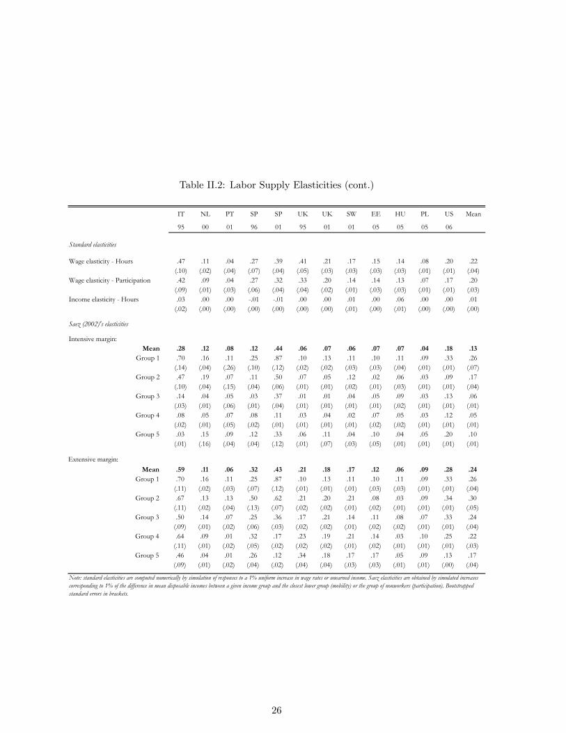
Table II.2: Labor Supply Elasticities (cont.)

IT NL PT SP SP UK UK SW EE HU PL US Mean

95 00 01 96 01 95 01 01 05 05 05 06

Standard elasticities

Wage elasticity ­ Hours .47 .11 .04 .27 .39 .41 .21 .17 .15 .14 .08 .20 .22(.10) (.02) (.04) (.07) (.04) (.05) (.03) (.03) (.03) (.03) (.01) (.01) (.04)

Wage elasticity ­ Participation .42 .09 .04 .27 .32 .33 .20 .14 .14 .13 .07 .17 .20(.09) (.01) (.03) (.06) (.04) (.04) (.02) (.01) (.03) (.03) (.01) (.01) (.03)

Income elasticity ­ Hours .03 .00 .00 ­.01 ­.01 .00 .00 .01 .00 .06 .00 .00 .01(.02) (.00) (.00) (.00) (.00) (.00) (.00) (.01) (.00) (.01) (.00) (.00) (.00)

Saez (2002)'s elasticities

Intensive margin:Mean .28 .12 .08 .12 .44 .06 .07 .06 .07 .07 .04 .18 .13

Group 1 .70 .16 .11 .25 .87 .10 .13 .11 .10 .11 .09 .33 .26(.14) (.04) (.26) (.10) (.12) (.02) (.02) (.03) (.03) (.04) (.01) (.01) (.07)

Group 2 .47 .19 .07 .11 .50 .07 .05 .12 .02 .06 .03 .09 .17(.10) (.04) (.15) (.04) (.06) (.01) (.01) (.02) (.01) (.03) (.01) (.01) (.04)

Group 3 .14 .04 .05 .03 .37 .01 .01 .04 .05 .09 .03 .13 .06(.03) (.01) (.06) (.01) (.04) (.01) (.01) (.01) (.01) (.02) (.01) (.01) (.01)

Group 4 .08 .05 .07 .08 .11 .03 .04 .02 .07 .05 .03 .12 .05(.02) (.01) (.05) (.02) (.01) (.01) (.01) (.01) (.02) (.02) (.01) (.01) (.01)

Group 5 .03 .15 .09 .12 .33 .06 .11 .04 .10 .04 .05 .20 .10(.01) (.16) (.04) (.04) (.12) (.01) (.07) (.03) (.05) (.01) (.01) (.01) (.01)

Extensive margin:Mean .59 .11 .06 .32 .43 .21 .18 .17 .12 .06 .09 .28 .24

Group 1 .70 .16 .11 .25 .87 .10 .13 .11 .10 .11 .09 .33 .26(.11) (.02) (.03) (.07) (.12) (.01) (.01) (.01) (.03) (.03) (.01) (.01) (.04)

Group 2 .67 .13 .13 .50 .62 .21 .20 .21 .08 .03 .09 .34 .30(.11) (.02) (.04) (.13) (.07) (.02) (.02) (.01) (.02) (.01) (.01) (.01) (.05)

Group 3 .50 .14 .07 .25 .36 .17 .21 .14 .11 .08 .07 .33 .24(.09) (.01) (.02) (.06) (.03) (.02) (.02) (.01) (.02) (.02) (.01) (.01) (.04)

Group 4 .64 .09 .01 .32 .17 .23 .19 .21 .14 .03 .10 .25 .22(.11) (.01) (.02) (.05) (.02) (.02) (.02) (.01) (.02) (.01) (.01) (.01) (.03)

Group 5 .46 .04 .01 .26 .12 .34 .18 .17 .17 .05 .09 .13 .17(.09) (.01) (.02) (.04) (.02) (.04) (.04) (.03) (.03) (.01) (.01) (.00) (.04)

Note: standard elasticities are computed numerically by simulation of responses to a 1% uniform increase in wage rates or unearned income. Saez elasticities are obtained by simulated increasescorresponding to 1% of the difference in mean disposable incomes between a given income group and the closest lower group (mobility) or the group of nonworkers (participation). Bootstrappedstandard errors in brackets.

26