Auton Robot (2013) 34:133–148DOI 10.1007/s10514-013-9327-2

Comparing ICP variants on real-world data setsOpen-source library and experimental protocol

François Pomerleau · Francis Colas ·Roland Siegwart · Stéphane Magnenat

Received: 28 May 2012 / Accepted: 22 January 2013 / Published online: 14 February 2013© Springer Science+Business Media New York 2013

Abstract Many modern sensors used for mapping produce3D point clouds, which are typically registered together usingthe iterative closest point (ICP) algorithm. Because ICP hasmany variants whose performances depend on the environ-ment and the sensor, hundreds of variations have been pub-lished. However, no comparison frameworks are available,leading to an arduous selection of an appropriate variantfor particular experimental conditions. The first contributionof this paper consists of a protocol that allows for a com-parison between ICP variants, taking into account a broadrange of inputs. The second contribution is an open-sourceICP library, which is fast enough to be usable in multiplereal-world applications, while being modular enough to easecomparison of multiple solutions. This paper presents twoexamples of these field applications. The last contribution isthe comparison of two baseline ICP variants using data setsthat cover a rich variety of environments. Besides demon-strating the need for improved ICP methods for natural,unstructured and information-deprived environments, thesebaseline variants also provide a solid basis to which novelsolutions could be compared. The combination of our proto-col, software, and baseline results demonstrate convincinglyhow open-source software can push forward the research inmapping and navigation.

F. Pomerleau (B) · F. Colas · R. Siegwart · S. MagnenatAutonomous System Lab, ETH Zurich,Tannenstrasse 3, 8092 Zurich, Switzerlande-mail: f.pomerleau@gmail.com

F. Colase-mail: francis.colas@mavt.ethz.ch

R. Siegwarte-mail: rsiegwart@ethz.ch

S. Magnenate-mail: stephane@magnenat.net

Keywords Experimental protocol · Iterative closest point ·Registration · Open-source · SLAM · Mapping

1 Introduction

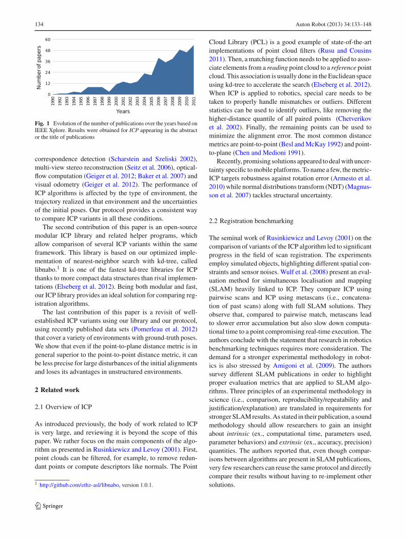
Laser-range sensors were a cornerstone to the developmentof mapping and navigation in the past two decades. Nowa-days, rotating laser scanners, stereo cameras or depth cam-eras (RGB-D) can provide dense 3D point clouds at a highfrequency. Using the iterative closest point (ICP) registrationalgorithm (Besl and McKay 1992; Chen and Medioni 1991),these point clouds can be matched to deduce the transfor-mation between them and, consequently, the 6 degrees offreedom motion of the sensor. Albeit originally proposedfor object reconstruction, the robotics field has extensivelyapplied registration for global scene reconstruction. ICP isa popular algorithm due to its simplicity: its general idea iseasy to understand and to implement. However, the basicalgorithm works well only in ideal cases. This led to hun-dreds of variations (around 400 papers published in the past20 years, see Fig. 1) around the original algorithm that weredemonstrated on different and incommensurable experimen-tal scenarios. This highlights both the usefulness of ICP andthe difficulty of finding a versatile version. Because thereexists no comparison framework, the selection of an appro-priate variant for particular experimental conditions is diffi-cult. This is a major problem because registration is at thefront-end of the mapping pipeline, and its selection affectsarbitrarily the results of all subsequent steps. There is there-fore a need for streamlining the selection of a registrationalgorithm given a type of environment.

The first contribution of this paper is a protocol to allowcomparison between ICP variants. This protocol encom-passes an experimental methodology and evaluation met-rics, as already proposed in other fields such as stereo

123

134 Auton Robot (2013) 34:133–148

Fig. 1 Evolution of the number of publications over the years based onIEEE Xplore. Results were obtained for ICP appearing in the abstractor the title of publications

correspondence detection (Scharstein and Szeliski 2002),multi-view stereo reconstruction (Seitz et al. 2006), optical-flow computation (Geiger et al. 2012; Baker et al. 2007) andvisual odometry (Geiger et al. 2012). The performance ofICP algorithms is affected by the type of environment, thetrajectory realized in that environment and the uncertaintiesof the initial poses. Our protocol provides a consistent wayto compare ICP variants in all these conditions.

The second contribution of this paper is an open-sourcemodular ICP library and related helper programs, whichallow comparison of several ICP variants within the sameframework. This library is based on our optimized imple-mentation of nearest-neighbor search with kd-tree, calledlibnabo.1 It is one of the fastest kd-tree libraries for ICPthanks to more compact data structures than rival implemen-tations (Elseberg et al. 2012). Being both modular and fast,our ICP library provides an ideal solution for comparing reg-istration algorithms.

The last contribution of this paper is a revisit of well-established ICP variants using our library and our protocol,using recently published data sets (Pomerleau et al. 2012)that cover a variety of environments with ground-truth poses.We show that even if the point-to-plane distance metric is ingeneral superior to the point-to-point distance metric, it canbe less precise for large disturbances of the initial alignmentsand loses its advantages in unstructured environments.

2 Related work

2.1 Overview of ICP

As introduced previously, the body of work related to ICPis very large, and reviewing it is beyond the scope of thispaper. We rather focus on the main components of the algo-rithm as presented in Rusinkiewicz and Levoy (2001). First,point clouds can be filtered, for example, to remove redun-dant points or compute descriptors like normals. The Point

1 http://github.com/ethz-asl/libnabo, version 1.0.1.

Cloud Library (PCL) is a good example of state-of-the-artimplementations of point cloud filters (Rusu and Cousins2011). Then, a matching function needs to be applied to asso-ciate elements from a reading point cloud to a reference pointcloud. This association is usually done in the Euclidean spaceusing kd-tree to accelerate the search (Elseberg et al. 2012).When ICP is applied to robotics, special care needs to betaken to properly handle mismatches or outliers. Differentstatistics can be used to identify outliers, like removing thehigher-distance quantile of all paired points (Chetverikovet al. 2002). Finally, the remaining points can be used tominimize the alignment error. The most common distancemetrics are point-to-point (Besl and McKay 1992) and point-to-plane (Chen and Medioni 1991).

Recently, promising solutions appeared to deal with uncer-tainty specific to mobile platforms. To name a few, the metric-ICP targets robustness against rotation error (Armesto et al.2010) while normal distributions transform (NDT) (Magnus-son et al. 2007) tackles structural uncertainty.

2.2 Registration benchmarking

The seminal work of Rusinkiewicz and Levoy (2001) on thecomparison of variants of the ICP algorithm led to significantprogress in the field of scan registration. The experimentsemploy simulated objects, highlighting different spatial con-straints and sensor noises. Wulf et al. (2008) present an eval-uation method for simultaneous localisation and mapping(SLAM) heavily linked to ICP. They compare ICP usingpairwise scans and ICP using metascans (i.e., concatena-tion of past scans) along with full SLAM solutions. Theyobserve that, compared to pairwise match, metascans leadto slower error accumulation but also slow down computa-tional time to a point compromising real-time execution. Theauthors conclude with the statement that research in roboticsbenchmarking techniques requires more consideration. Thedemand for a stronger experimental methodology in robot-ics is also stressed by Amigoni et al. (2009). The authorssurvey different SLAM publications in order to highlightproper evaluation metrics that are applied to SLAM algo-rithms. Three principles of an experimental methodology inscience (i.e., comparison, reproducibility/repeatability andjustification/explanation) are translated in requirements forstronger SLAM results. As stated in their publication, a soundmethodology should allow researchers to gain an insightabout intrinsic (ex., computational time, parameters used,parameter behaviors) and extrinsic (ex., accuracy, precision)quantities. The authors reported that, even though compar-isons between algorithms are present in SLAM publications,very few researchers can reuse the same protocol and directlycompare their results without having to re-implement othersolutions.

123

Auton Robot (2013) 34:133–148 135

Registration quality depends on many external factors.Typically, a single type of environment is selected for evalu-ation. The latter is mostly urban (Pathak et al. 2010; Wulfet al. 2008) or well-structured environment, like tunnels(Magnusson et al. 2009). The robustness of registrationagainst initial misalignment is explored in Hugli and Schutz(1997). This type of exploration is continued with an eval-uation of ICP against NDT in order to compare the valleyof convergence of both methods (Magnusson et al. 2009).In the work of Pathak et al. (2010), the sensitivity of theirregistration algorithm to low spatial overlap is identified andused to predict scan-matching failures.

When presenting registration results, authors face theproblem of reducing the dimensionality of their results tolow-dimension and meaningful performance metrics. Earlywork mainly focuses on the rapidity of convergence and thefinal accuracy of different solutions (Rusinkiewicz and Levoy2001). Typical parameters of interest concern translation androtation for a total of six dimensions. While summarizing thetranslation components using the Euclidean distance is com-monly accepted, different methods are used for the rotation.The work of Wulf et al. (2008) mixes scans in 3D (928 scansover 1 km) with ground-truth poses in 2D. Consequently,the evaluation is done in 2D using Euclidean distance fortranslation errors and absolute value of the orientation dif-ferences. To produce statistics about the overall experiment,the authors propose to use the standard deviation of all errorsand the maximum error as evaluation metrics. Doing theirevaluation directly in 3D, Tong et al. (2012) define two sep-arate root-mean-squared (RMS) errors (i.e., one on transla-tion and another on rotation components). For both errors,they employ the Euclidean distance between the computedposes and the ground-truth poses, using a rotation vectorparametrization for the orientation. Addressing the problemof multiple rotation metrics, Huynh (2009) proposes an eval-uation of six different types of distance for SO(3) used inthe scientific literature. She concludes that the norm of thedifference of Euler Angles is not a distance and that the useof geodesic distance on a unit sphere is preferable. Insteadof using continuous metrics, Hugli and Schutz (1997) pro-pose to use Successful Initial Configuration map, or SIC-map, to display results on a 2D plot. The authors used fixedthresholds on the error to identify failure, weak success andsuccess of the registration. The SIC-maps help to visual-ize the convergence region but limit the number of sam-ples that can be tested. This type of result representationalso makes comparison between different variants difficult todisplay.

In this paper, we applied the principles proposed byAmigoni et al. (2009) to a subset of the SLAM problem:scan registration. In light of the recent work on registra-tion, we aimed to bring those different evaluation types intothe same protocol. This protocol should enhance deeper

investigation of registration algorithms by considering (1)a set of external factors and (2) a set of performancemetrics.

3 Method

In this section, we highlight the different elements that influ-ence the outcome of ICP variants and that can be controlledin order to evaluate those variants. We also introduce robustmetrics that we consider for a quantitative assessment of thealgorithm.

3.1 Sensitivity to input

ICP takes two scans as input with an initial alignment of onewith respect to the other. As ICP is an approximate algo-rithm essentially doing local convergence, its result dependson the initial pose. This initial guess is typically provided byinertial-measurement accumulation, odometry or heuristicmotion models, which all have limited precision and increas-ing uncertainty with time between observations. It is there-fore important to assess how well an ICP solution convergesclose to the correct pose based on various initial hypothe-ses. To this aim, we propose to sample the space of initialalignment by adding perturbations to a ground-truth value.While the error distribution of odometry models is usuallynot Gaussian for non-linear kinematic models, the deviationfrom a Gaussian depends on the actual model and commandhistory, which goes beyond the scope of our data sets. Asa reasonable approximation, we sampled the perturbationsfrom zero-mean 6D multivariate Gaussian distribution.

Another factor driving the difficulty of scan matching isthe amount of outliers. If there are a lot of points that donot correspond to the same features in both scans, ICP runsthe risk of converging to a local optimum driven by falsematches. We quantified this phenomenon by assessing theoverlap ratio of a scan with respect to another (outlier ratiois the complement of the overlap ratio). More formally, theoverlap is defined by the ratio of points of a scan A for whichthere is a matching point in a second scan B. Points are con-sidered as matching in this case if they lie within a distancelimit that decreases with the local density of points.

In robotics, this overlap is primarily governed by thefield of view and the motion of the sensor. Indeed, with-out dynamic elements in the scene, the overlap correspondsmainly to the ratio between the intersection of sensor fieldsof view on the one hand, and the field of view of the referencepoint cloud on the other hand. If the motion, especially forrotation, is large when compared to the field of view, then theoverlap can be too low for ICP to converge properly. For slowsensors, like 2D laser scanners generating 3D point cloudsby rotating around an axis, it is therefore preferable to do

123

136 Auton Robot (2013) 34:133–148

scan matching for each consecutive pair of scans. However,on faster sensors like RGB-D cameras running up to 30 Hz,it is often possible and even desirable to skip several scans,as long as the overlap does not fall too low.

Finally, the content of the scans themselves can have ahuge influence on the registration quality. Indoor environ-ments typically exhibit a lot of planar surfaces (e.g. ground,walls, ceiling, tables) that are therefore locally regular. Inthat case, if the matching step is slightly wrong, a wronglyassociated point still has a good chance of behaving like thecorrect point. On the other hand, natural environments withtrees, bushes and herbs will have false matches detrimentalto the error minimization. Moreover, environments without areasonable ratio of horizontal and vertical objects might lackinformation for proper registration. This typically happensin long and straight hallway or outside on open space wherethe ground is the major surface present.

3.2 Evaluation metrics

For each ICP solution, initial alignments (i.e. being theground truth plus perturbation) is applied to all selectedpairs of scans. At the end, the evaluation produces samplesfrom the distribution of resulting alignments for each pair ofscans. Then, cumulating error distributions over all pairs ofscans eases the analysis of samples from that particular ICPsolution for a given environment and a given perturbationlevel. We can also accumulate over the different environ-ments for the marginal distribution of error of a given ICPsolution.

However, this distribution lies in SE(3), the specialEuclidean group in dimension 3, whereas we are mainlyinterested in both the translation and rotation. Therefore, weprojected the 6D distribution into the translation and rotationerrors. Given the ground-truth transformation expressed by a4×4 homogeneous matrix Tg and its corresponding transfor-mation found by the registration solution Tr , we can definethe remaining error ΔT as follows:

ΔT =[ΔR Δt

0 1

]= Tr T −1

g (1)

with its translation error et , defined as the Euclidean normof translation vector Δt :

et = ‖Δt‖ =√

Δx2 + Δy2 + Δz2 (2)

and its rotation error er , defined as the Geodesic distancedirectly from the rotation matrix ΔR:

er = arccos

(trace(ΔR) − 1

2

)(3)

In order to compare these distributions, we used robuststatistics like the median and the quantiles instead of mean

and covariance. Indeed, as the error distributions are farfrom Gaussians, the empirical mean and covariance are notreally indicative values for interpreting precision and accu-racy. This choice is similar to May et al. (2009), wherethe authors defined A50, A75, A95 as the respective quan-tiles for probabilities 0.5 (i.e. the median), 0.75 and 0.95of the error distributions. Another advantage of these sta-tistics is that they allow interpretation in terms of accuracyand precision. The solution under evaluation is accurate ifthe values of A50, A75 and A95 are close to zero. Thesolution is precise if the difference between those quantilesare small.

Throughout this paper, we present the cumulative func-tion of the distribution of outcomes against the distance ofthe outcome with respect to ground truth. Those graphs thuspresent the proportion of outcomes that lie beneath a givenerror. Moreover, it is easy to see the value of this error foreach quantile. This type of representation was called Recall-Accuracy threshold in a previous work (Jian and Vemuri2011). An alternative presentation of those results is to showthe histogram of the number of outcomes for each error bin,which corresponds to the derivative of the cumulative thatwe propose. However, that presentation renders difficult thecomparison of many distributions and the depiction of theA50, A75 and A95 statistics.

Finally, the computing time can be an important fac-tor, especially for online applications with real-time con-straints and embedded systems with limited processingpower. It is however challenging to get an absolute eval-uation of the computing time that is relevant for differenthardware and different use cases. The choice of program-ming language, the technical level of the programmers,the amount of parallelism, etc., are all elements that couldaffect time performance. In general, time evaluation shouldbe considered as qualitative measurement unless all thoseelements are controlled and known to be as uniform aspossible.

3.3 Protocol

With those metrics, we can now propose a protocol for theevaluation of ICP variants that goes beyond parameter iden-tifications.

First, variants should always be compared to a commonlyaccepted ICP baseline. This contrasts with papers that com-pare novel variants between themselves in order to highlight aspecific hypothesis. While we recognize the interest of theseworks, the amount of ICP variants presented in the literaturecalls for more effort to relate them. In Sect. 5.2, we analyzetwo classical variants that we considered reasonable choicesfor ICP baselines.

123

Auton Robot (2013) 34:133–148 137

Fig. 2 The modular ICP chainas implemented inlibpointmatcher. Notethat some data filters are appliedto the reading once and some areapplied at each iteration step

Table 1 List of processing blocks available in libpointmatcher

Current module implementations

Data filtering FixStepSampling, MaxDensity,MaxPointCount,MaxQuantileOnAxis, MinDist,ObservationDirection,OrientNormals, RandomSampling,RemoveNaN,SamplingSurfaceNormal, Shadow,SimpleSensorNoise,SurfaceNormal

Data association KDTree, KDTreeVarDist

Outlier filtering MaxDist, MedianDist,MinDist,SurfaceNormal,TrimmedDist,VarTrimmedDist

Error minimization PointToPlane, PointToPoint

Transformation checking Bound, Counter, Differential

Inspection Performance, VTKFile

Log File

This list displays the status of the library as of version 1.0.0 and isintended to evolve over time

Second, ICP variants need to be compared on enough datain order to reduce the risk of overfitting and to ensure statisti-cally significant interpretations. Specific fields of applicationmay require specialized data sets, but efforts should be madeto also compare on generic data sets. To obtain a comparisonas unbiased as possible, the data should cover different kindsof environments at different overlap levels. In this paper, wepropose to employ a group of 3D robotics data sets coveringa variety of environments. Moreover, algorithms should becompared with different perturbation distributions in orderto assess their robustness. We propose three different per-turbation levels (easy, medium and hard) according to thecharacteristics of the data set (mainly the scale of the ele-ments in the environment and the noise of the sensor).

Finally, the actual comparison should be made withrespect to the distribution of errors rather than being madejust on a single result. We propose to use quantiles as robuststatistics to quantitatively describe and compare the differentresults.

4 Modular ICP

ICP is an iterative algorithm performing several sequentialprocessing steps, both inside and outside its main loop. Foreach step, there exist several strategies, and each strategydemands specific parameters.

To our knowledge, there is currently no software toolto compare these strategies. The PCL has a partial supportfor filters in its registration pipeline, but not a completelyreconfigurable ICP chain.2 To enable such a comparison,we have developed a modular ICP chain, as illustrated inFig. 2, and made it available as open source in the form ofthe libpointmatcher library.3 This library is written inC++11, restricted to the subset supported by GCC 4.4 andmore recent versions. In the ICP chain, every module is aclass that can describe its own possible parameters, there-fore enabling the whole chain to be configured at run timeusing YAML (Ben-Kiki et al. 2009). This text-based config-uration aids to explicit parameters used and eases the sharingof working setups with others, which ultimately allows forreproducibility and reusability of the solutions. Table 1 liststhe available modules.

Our ICP chain takes as input two point clouds, in 2D or 3D,and estimates the translation and the rotation parameters thatminimize the alignment error. We called the first point cloudthe reference and the second the reading. The ICP algorithmtries to align the reading onto the reference. To do so, itfirst applies filtering to the point clouds, and then it iteratesthrough a sequence of processing blocks. For each iteration, itassociates points in reading to points in reference and finds atransformation of reading that minimizes the alignment error.

4.1 Processing blocks

More specifically, the ICP chain consists of several steps,implemented by modules. The steps and the correspondingtypes of modules are:

2 We are in contact with PCL developers to integrate parts of our workinto it.3 http://github.com/ethz-asl/libpointmatcher, version 1.0.0 at time ofsubmission of this paper.

123

138 Auton Robot (2013) 34:133–148

– Data filtering This step applies to both the referenceand the reading point clouds. At this step, zero or moreDataPointsFilter modules take a point cloud asinput, transform it and produce another cloud as output.The transformation might add information, for instancesurface normals, or might change the number of points,for instance by randomly removing some of them.

– Transformation The reading point cloud is rotated andtranslated. Additional data, such as surface normals, aretransformed as well.

– Data association A Matchermodule links points in thereading to points in the reference. Currently, we providea fast k–nearest-neighbor matcher based on a kd-tree,using libnabo.

– Outlier filtering Zero or more OutlierFilter mod-ules remove (hard rejection) and/or weight (soft rejec-tion) links between points in the reading and theirmatched points in the reference. Criteria can be a fixedmaximum authorized distance, a factor of the mediandistance, etc. Points with zero weights are ignored in thesubsequent minimization step.

– Error minimization An ErrorMinimizer modulecomputes a transformation matrix to minimize the errorbetween the reading and the reference. Different errorfunctions are available, such as point-to-point and point-to-plane.

– Transformation checking Zero or moreTransformationChecker modules can stop theiteration depending on some conditions. For example,a condition can be the number of times the loop was exe-cuted, or it can be related to the matching error. Becausethe modules can be chained, we defined that the relationbetween modules must agree through an OR-condition,while all AND-conditions are defined within a singlemodule.

4.2 Data types

The ICP chain provides standardized interfaces between eachstep. This allows for the addition of novel algorithms to somesteps to evaluate their effect on the global ICP behavior. Theseinterfaces are:

– The DataPoints class represents a point cloud. Forevery point, it has features and, optionally, descriptors.Features are typically the coordinates of the point in thespace. Descriptors contain information attached to thepoint, such as its color, its normal vector, etc. In bothfeatures and descriptors, every point can have multiplechannels. Every channel has a dimension and a name.For instance, a typical 3D cloud might have the chan-nels “x”, “y”, “z”, “w” of dimension 1 as features (using

homogeneous coordinates), and the channel “normal” ofsize 3 as descriptor. There are no sub-channels, such as“normal.x”, for the sake of simplicity. Moreover, the posi-tion of the points is in homogeneous coordinates becausethey need both translation and rotation, while the normalsneed only rotation. All channels contain scalar values ofthe scalar type from the template parameter. Althoughthis might be sub-optimal in memory, it eases a lot theinteraction between the different modules.

– The Matches class is the result of the data-associationstep, before outlier rejection. It corresponds to a list ofassociated reference identifiers, along with the corre-sponding squared distance, for all points in the reading.A single point in the reading can have one or multiplematches.

– The OutlierWeights class contains the weights ofthe associations between the points in Matches and thepoints in the reference. A weight of 0 means no asso-ciation, while a weight of 1 means a complete trust inassociation.

– The TransformationParameters is a transfor-mation in the special Euclidean group of dimensionn, SE(n), implemented as a matrix of size n +1×n +1.

4.3 Implementation

All modules are children of parent classes defined withinthe PointMatcher class. This class is templatized onthe scalar type for the point coordinates, typically floator double. Additionally, the PointMatcherSupportnamespace hosts classes that do not depend on the templateparameter. Every kind of module has its own pair of .h and.cpp files. Because modules can enumerate their parametersat run time, only the parent classes lie in the publicly acces-sible headers. This maintains a lean and easy-to-learn appli-cation programming interface (API).

To use libpointmatcher from a third-party program,the two classes ICP and ICPSequence can be instanti-ated. The first provides a basic registration between a readingand a reference, given an initial transformation. The secondprovides a tracker-style interface: an instance of this classreceives several point clouds in sequence and continuouslyupdates the transformation with respect to a user-providedpoint cloud. This is useful to limit drift due to noise in thecase of high-frequency sensors (Pomerleau et al. 2011). Acommon base class, ICPChainBase, holds the instancesof the modules and provides the loading mechanism.

When doing research, it is crucial to understand whatis going on, in particular in complex processing pipelineslike the ICP chain. Therefore, libpointmatcher pro-vides two inspection mechanisms: the logger and the inspec-tor. The logger is responsible for writing information during

123

Auton Robot (2013) 34:133–148 139

Table 2 Configurations of ICP chains for the Kinect tracker and the 7-floor mapping applications

Step Module Description

Kinect tracker Data filtering of reference MaxDist Keep points closer than 7 m

SamplingSurfaceNormal Random sub-sampling, typically keep 20 %

Data filtering of reading MaxDist Keep points closer than 7 m

RandomSampling Sub-sampling 17× and normal extraction

Data association KDTree kd-tree matching with 0.1 m max. distance

Outlier filtering TrimmedDist Keep 85 % closest points

Error minimization PointToPlane Point-to-plane

Transformation checking Differential Min. error below 1 cm and 0.001 rad

Counter Iteration count reached 30

Bound Transformation beyond bounds

7-Floor mapping Data filtering of reference SurfaceNormal Extraction of surface normal vectors

RandomSampling Random sub-sampling, keep 50 %

Data filtering of reading SurfaceNormal Extraction of surface normal vectors

UniformizeDensity Keep uniform density

Data association KDTree kd-tree matching with 0.5 m max. distance

Outlier filtering TrimmedDist Keep 95 % closest points

SurfaceNormal Remove when normals are more than 45◦ off

Error minimization PointToPlane Point-to-plane

Transformation checking Differential Min. error below 1 cm and 0.001 rad

Counter Iteration count reached 30

Bound Transformation beyond bounds

execution to a file or to the console. It will typically displaylight statistics and warnings. The inspector provides deeperscrutiny than the logger. There are several instances of inspec-tors in libpointmatcher. For instance, one dumps ICPoperations as VTK files (Schroeder et al. 2006), allowingto visualize the inner loop of the algorithm frame by frame.Another inspector collects statistics for performance evalua-tion.

5 Evaluation

In this section, we show how we applied libpoint-matcher to two relatively different cases of scan matching:a fast RGB-D camera and a rolling 2D lidar, demonstratingthe genericity of our modular ICP chain. In a second part, wegive new insights on well-accepted ICP variants using ourcomparison protocol.

5.1 Applications based on the modular ICP chain

The first application consists of estimating the pose of aKinect RGB-D sensor in a home-like environment in real-time (30 Hz). Using theICPSequence class of our modularICP library, this tracker integrates with ROS and publishesthe 3D pose as tf, the standard way to describe transfor-

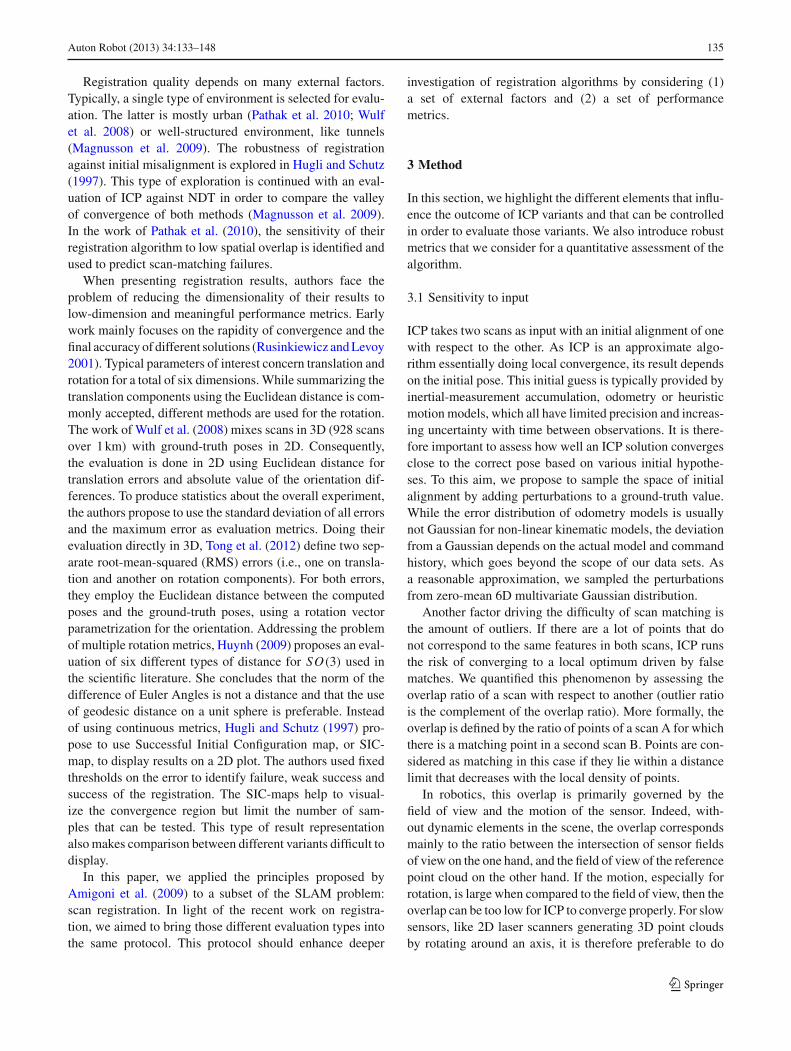
mations between reference frames in ROS. We exploreddifferent parameters related to point-cloud filtering forsensor-noise rejection, the selection of sub-sampling meth-ods and the approximation for the nearest-neighbor search.We first left out points beyond 7 m because these are verynoisy with the Kinect. We then sub-sampled the reading ran-domly, typically keeping 20 % of the 3D points generatedfrom of a 160×120 depth image. For the reference, we usedthe SamplingSurfaceNormal module that efficientlycombines sub-sampling and normal generation. This moduledecomposes the point-cloud space in boxes, by recursivelysplitting the cloud through axis-aligned hyperplanes in sucha way as to maximize the evenness of the aspect ratio of theboxes. When the number of points in a box reaches a thresh-old value, the filter computes the center of mass of thesepoints and its normal by taking the eigenvector correspond-ing to the smallest eigenvalue of all points in the box. Thereference and the reading points are associated up to a dis-tance of 0.1 m using a kd-tree. As the Kinect works indoors,we performed point-to-plane error minimization. The upperpart of Table 2 summarizes the configuration of the ICP chainfor this application. The top of Fig. 3 shows one of the 27paths executed while being tracked in parallel with a Viconsystem. The Vicon was used to determine the ground truthposes during this evaluation. The bottom of Fig. 3 shows themain factor influencing the registration speed: the number of

123

140 Auton Robot (2013) 34:133–148

Fig. 3 Tracking the pose of a Kinect RGB-D sensor in a home-likeenvironment. Top Projection on the xy-plane of a tracked position (dark-red) versus the measured ground truth (light green). Each grid square ishalf a meter. Bottom Performance for different processors: Intel Core i7Q 820 (blue cross), Intel Xeon L5335 (red circles), and Intel Atom Z530(asterisk) (Color figure online)

points randomly sub-sampled for the reading, with real timeachieved with 4,000 points using a single core of a laptopCore i7 Q 820 processor. About 1,700 points are sufficientfor high-quality tracking, which is achievable in real time onan old Intel Xeon L5335. An Atom can run at about 10 Hz,with enough points for approximate tracking. The completeresults are available in a previous paper (Pomerleau et al.2011). This experiment shows that our library can scale on alarge range of computational power and provide high-quality,real-time tracking on current average hardware.

The second application is the mapping of a seven-floorstaircase with a search-and-rescue robot (Fig. 4). This robot isequipped with tracks and flippers to increase the motion capa-bilities. However, this implies that the motion estimated fromthe tracks encoder is highly unreliable, even on flat ground.The robot has a 2D laser scanner mounted on a horizontalaxis, allowing it to roll back and forth to acquire 3D scans infront of the robot. In this application, the robot acquires scanswith a stop-and-go strategy. The robot maintains an onboardmap of the environment (600 k points) that was processedonline. When a new scan was available, the robot performedICP with this map as reference and the scan as reading, like

metascan used in Wulf et al. (2008). As this is an office envi-ronment, we used a point-to-plane variant, which implies thatwe extracted the normals of the points prior to each registra-tion. The points were associated up to a distance of 0.5 musing a kd-tree. As there was a low expectation of encoun-tering dynamic elements, the 95 % closest points were kept.However, matched points with surface normal vectors differ-ing by more than 45◦ are discarded. This prevented the pointsfrom the ceiling from being matched with the points from thefloor above, which would distort the whole map by havingfloors without thickness. The bottom part of Table 2 summa-rizes the configuration of the ICP chain. Note that there is noglobal relaxation or loop closure; the parallel floors visiblein Fig. 4 are due solely to good registration quality.

Both examples demonstrate the added value of modularICP chains as they have different requirements that can stillbe fulfilled with the same open-source ICP library.

5.2 Revisiting well-established ICP variants

In this section, we demonstrate our evaluation protocol ontwo well-established ICP variants. We have implementedboth of them using our library before applying them to differ-ent environments. They can provide a fair baseline to whichnew algorithms can be compared. Furthermore, this showsthe relation between environment type, ICP distance metricand convergence performances.

5.2.1 Data sets

We selected six different environments from the “Challeng-ing Laser Registration” data sets (Pomerleau et al. 2012).These data sets4 include ground-truth poses and cover a broadrange of applications and conditions, including dynamic out-liers such as people walking in the range of the laser whileit is scanning. Each data set consists of around 30 full 3Dscans. The scans were taken with an Hokuyo UTM-30LX2D laser range sensor mounted on a tilting platform. Theground-truth poses of the platform were tracked with milli-metric precision using a theodolite. Table 3 summarizes thefeatures of the selected data sets: Apartment (Fig. 5) ETH,Stairs, Wood (in summer), Gazebo (in winter, see Fig. 6),and Mountain Plain. These six data sets cover various typesof environments: artificial and natural, cluttered and open,homogeneous and highly variable.

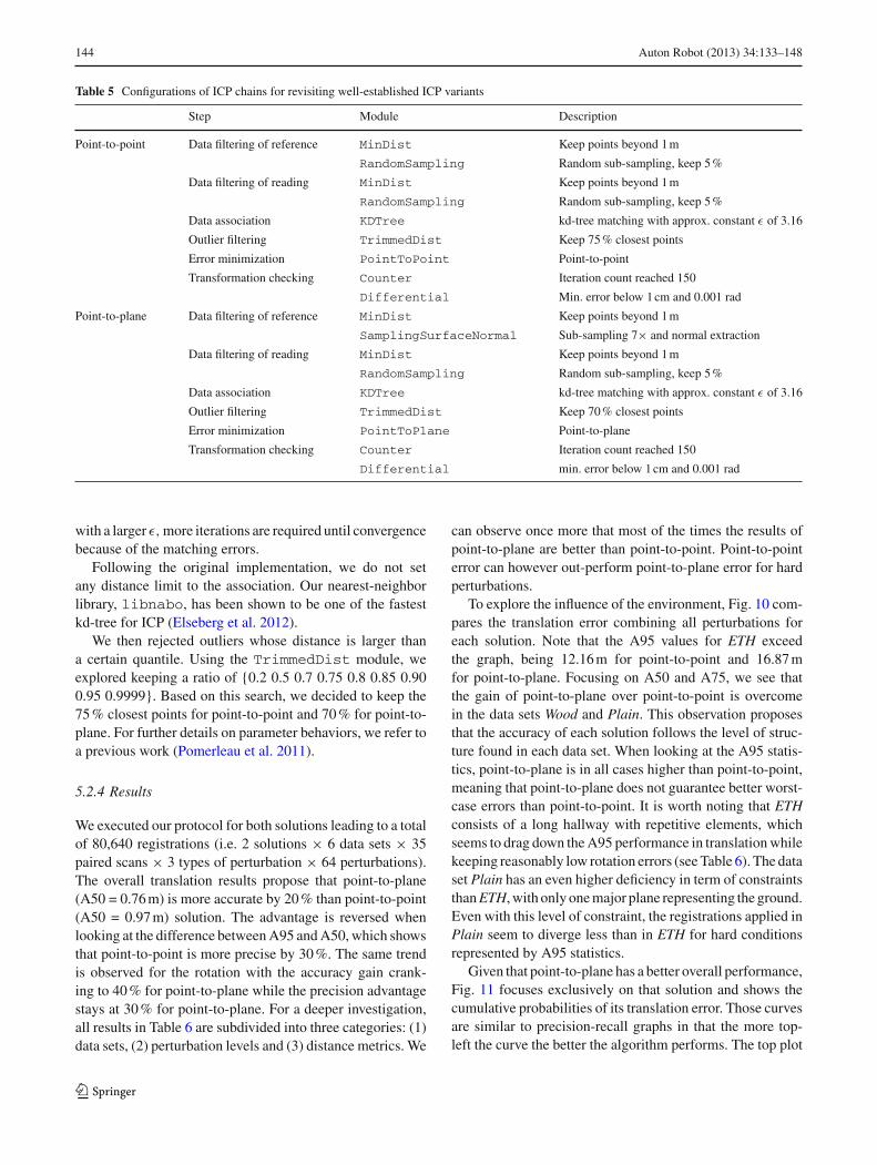
Figure 7 shows the overlap between each pair of scans inall data sets. First, one can see that the overlap is not exactlysymmetric. Indeed, if a scan is smaller than the other, allits points will find a match in the second, but not the otherway around. Second, Apartment and Stairs show clusters

4 http://projects.asl.ethz.ch/datasets/doku.php?id=laserregistration:laserregistration.

123

Auton Robot (2013) 34:133–148 141

Fig. 4 Mapping of a seven-floor staircase using a search-and-rescuerobot. Left Side view of the resulting map with the floor colored basedon elevation. Middle Top view of the E floor with the ceiling removed

and the points colored based on elevation. Right Photograph of the robotwith climbing capability (Color figure online)

Table 3 Characteristics of the six data sets used to revisit well-established ICP variants

Name Description Nbr. Pt. per Poses Scenescans scan bounding box (m) bounding box (m)

Apartment Single floor with five rooms 45 365 k 5 × 5 × 0.06 17 × 10× 3Stairs Small staircase transitioning from indoor to outdoor 31 191 k 10 × 3 × 2.50 21 × 111 × 27ETH Large hallway with pillars and arches 36 191 k 24 × 2 × 0.50 62 × 65 × 18Gazebo (winter) Wine trees covering a gazebo in a public park 32 153 k 4 × 5 ×0.09 72 × 70 × 19Wood (summer) Dense vegetation around a small paved way 37 182 k 10 × 15 × 0.50 30 × 53 × 20Plain Small concave basin with alpine vegetations 31 102 k 18 × 6 × 2.70 36 × 40 × 8

Fig. 5 Overview of the Apartment data set. Left Photograph of thekitchen. Middle Top view of the point clouds with the ceiling removed.The color of the points shows their elevation: high points are in darkblue, low points are in light gray. The yellow lines with black dots

represent the path of the scanner through the apartment. Top right Pho-tograph of the living room. Bottom right Photograph of the bedroom(Color figure online)

123

142 Auton Robot (2013) 34:133–148

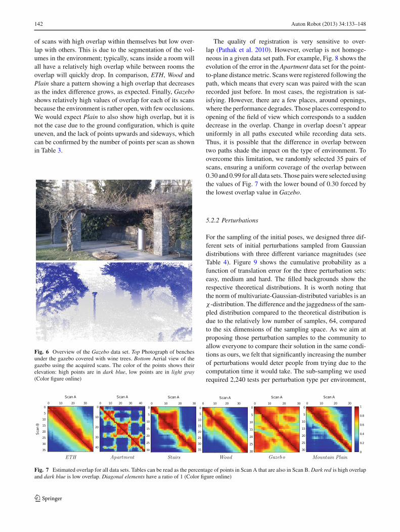
of scans with high overlap within themselves but low over-lap with others. This is due to the segmentation of the vol-umes in the environment; typically, scans inside a room willall have a relatively high overlap while between rooms theoverlap will quickly drop. In comparison, ETH, Wood andPlain share a pattern showing a high overlap that decreasesas the index difference grows, as expected. Finally, Gazeboshows relatively high values of overlap for each of its scansbecause the environment is rather open, with few occlusions.We would expect Plain to also show high overlap, but it isnot the case due to the ground configuration, which is quiteuneven, and the lack of points upwards and sideways, whichcan be confirmed by the number of points per scan as shownin Table 3.

Fig. 6 Overview of the Gazebo data set. Top Photograph of benchesunder the gazebo covered with wine trees. Bottom Aerial view of thegazebo using the acquired scans. The color of the points shows theirelevation: high points are in dark blue, low points are in light gray(Color figure online)

The quality of registration is very sensitive to over-lap (Pathak et al. 2010). However, overlap is not homoge-neous in a given data set path. For example, Fig. 8 shows theevolution of the error in the Apartment data set for the point-to-plane distance metric. Scans were registered following thepath, which means that every scan was paired with the scanrecorded just before. In most cases, the registration is sat-isfying. However, there are a few places, around openings,where the performance degrades. Those places correspond toopening of the field of view which corresponds to a suddendecrease in the overlap. Change in overlap doesn’t appearuniformly in all paths executed while recording data sets.Thus, it is possible that the difference in overlap betweentwo paths shade the impact on the type of environment. Toovercome this limitation, we randomly selected 35 pairs ofscans, ensuring a uniform coverage of the overlap between0.30 and 0.99 for all data sets. Those pairs were selected usingthe values of Fig. 7 with the lower bound of 0.30 forced bythe lowest overlap value in Gazebo.

5.2.2 Perturbations

For the sampling of the initial poses, we designed three dif-ferent sets of initial perturbations sampled from Gaussiandistributions with three different variance magnitudes (seeTable 4). Figure 9 shows the cumulative probability as afunction of translation error for the three perturbation sets:easy, medium and hard. The filled backgrounds show therespective theoretical distributions. It is worth noting thatthe norm of multivariate-Gaussian-distributed variables is anχ -distribution. The difference and the jaggedness of the sam-pled distribution compared to the theoretical distribution isdue to the relatively low number of samples, 64, comparedto the six dimensions of the sampling space. As we aim atproposing those perturbation samples to the community toallow everyone to compare their solution in the same condi-tions as ours, we felt that significantly increasing the numberof perturbations would deter people from trying due to thecomputation time it would take. The sub-sampling we usedrequired 2,240 tests per perturbation type per environment,

Fig. 7 Estimated overlap for all data sets. Tables can be read as the percentage of points in Scan A that are also in Scan B. Dark red is high overlapand dark blue is low overlap. Diagonal elements have a ratio of 1 (Color figure online)

123

Auton Robot (2013) 34:133–148 143

Fig. 8 Point-to-plane solution in the Apartment data set: separate sta-tistics for every pose. The path of the scanner (green) with the A50and A75 statistics overlaid on a sketch of the environment (Color figureonline)

Table 4 Standard deviations on each component and number of sam-ples for each perturbation level

Translation (m) Rotation (◦) Nb. Samples

Easy 0.1 10 64

Medium 0.5 20 64

Hard 1.0 45 64

0 0.5 1 1.5 2 2.5 30

0.2

0.4

0.6

0.8

1

Initial perturbation distances (m)

Cum

ulat

ive

prob

abili

ty

Easy Sampled

Medium Sampled

Hard Sampled

Fig. 9 Cumulative probability as function of translation error for eachof the perturbation sets. The lines are based on the actual 64 samples;the filled backgrounds correspond to the theoretical curves. The easysampled and theoretical curves overlay due to scaling

which we consider to be a reasonable compromise betweenthe number of samples and the evaluation time.

A list of the selection of scans combined with the pre-computed perturbation for all data sets is available by direct

communication with the authors and will be accessible on aweb site for convenience in the near future.

5.2.3 Selection and optimization of ICP parameters

We wish to revisit two of the textbook ICP variants, usingpoint-to-point (Besl and McKay 1992) and point-to-plane(Chen and Medioni 1991) distance metrics, both combinedwith the trimmed-ICP outlier rejection (Chetverikov et al.2002). We have chosen these because they are the most com-pared and researchers need to re-implement them every time.We hope to accelerate the comparison process for more mod-ern solutions by providing those two baseline solutions in anopen-source library.

Albeit simple, they depend on a certain number of para-meters. We have fixed some and optimized others to allowfor an efficient convergence of the algorithm. Table 5 showsthe final values after optimization. We aimed at both mini-mizing the error and maximizing the performance, followingthe method described in a previous work (Pomerleau et al.2011).

Our ICP chain starts by sub-sampling both the referenceand the reading point clouds. In the case of point-to-point,both point clouds are sub-sampled with uniform probabil-ity using the RandomSampling module. We explored thespace of sub-sampling ratios using probabilities of keepingpoints in the range of {0.001, 0.01, 0.05, 0.1, 0.5, 1.0} for thereading and {0.001, 0.01, 0.05, 0.1, 1.0} for the reference. Inthe case of point-to-plane, because we wanted to extract thenormals, we used the SamplingSurfaceNormal mod-ule. We explore thresholds of sizes {5, 7, 10, 20, 100, 200}.For the reading, we used the same sub-sampling method asfor point-to-point, looking for ratios of {0.001, 0.01, 0.05,0.1, 0.5, 1}. After an exhaustive search, this optimizationreturns ratios of 0.05 for both the reference and the readingfor point-to-point, and a ratio of 0.05 for the reading and athreshold of 7 points for the reference for point-to-plane.

The matching step looks for the nearest neighbors of everypoint using a kd-tree. We use the KDTree module, whichhas three parameters: the number of nearest neighbors in thereference to associate to each point in the reading, an approx-imation factor ε allowing a maximum error of 1+ ε betweenthe returned nearest neighbor and the true nearest neigh-bor (Arya and Mount 1993) and a maximal distance beyondwhich neighbors are not considered any more. We use onlyone neighbor for the sake of simplicity. We choose a value of3.16 for ε because as shown in a previous work (Pomerleau etal. 2011), this value leads to the fastest registration.5 Indeed,with a smaller ε, nearest-neighbor queries take longer, and

5 The semantics of ε has been changed since Pomerleau et al. (2011)to be compatible with other open-source implementations.

123

144 Auton Robot (2013) 34:133–148

Table 5 Configurations of ICP chains for revisiting well-established ICP variants

Step Module Description

Point-to-point Data filtering of reference MinDist Keep points beyond 1 m

RandomSampling Random sub-sampling, keep 5 %

Data filtering of reading MinDist Keep points beyond 1 m

RandomSampling Random sub-sampling, keep 5 %

Data association KDTree kd-tree matching with approx. constant ε of 3.16

Outlier filtering TrimmedDist Keep 75 % closest points

Error minimization PointToPoint Point-to-point

Transformation checking Counter Iteration count reached 150

Differential Min. error below 1 cm and 0.001 rad

Point-to-plane Data filtering of reference MinDist Keep points beyond 1 m

SamplingSurfaceNormal Sub-sampling 7× and normal extraction

Data filtering of reading MinDist Keep points beyond 1 m

RandomSampling Random sub-sampling, keep 5 %

Data association KDTree kd-tree matching with approx. constant ε of 3.16

Outlier filtering TrimmedDist Keep 70 % closest points

Error minimization PointToPlane Point-to-plane

Transformation checking Counter Iteration count reached 150

Differential min. error below 1 cm and 0.001 rad

with a larger ε, more iterations are required until convergencebecause of the matching errors.

Following the original implementation, we do not setany distance limit to the association. Our nearest-neighborlibrary, libnabo, has been shown to be one of the fastestkd-tree for ICP (Elseberg et al. 2012).

We then rejected outliers whose distance is larger thana certain quantile. Using the TrimmedDist module, weexplored keeping a ratio of {0.2 0.5 0.7 0.75 0.8 0.85 0.900.95 0.9999}. Based on this search, we decided to keep the75 % closest points for point-to-point and 70 % for point-to-plane. For further details on parameter behaviors, we refer toa previous work (Pomerleau et al. 2011).

5.2.4 Results

We executed our protocol for both solutions leading to a totalof 80,640 registrations (i.e. 2 solutions × 6 data sets × 35paired scans × 3 types of perturbation × 64 perturbations).The overall translation results propose that point-to-plane(A50 = 0.76 m) is more accurate by 20 % than point-to-point(A50 = 0.97 m) solution. The advantage is reversed whenlooking at the difference between A95 and A50, which showsthat point-to-point is more precise by 30 %. The same trendis observed for the rotation with the accuracy gain crank-ing to 40 % for point-to-plane while the precision advantagestays at 30 % for point-to-plane. For a deeper investigation,all results in Table 6 are subdivided into three categories: (1)data sets, (2) perturbation levels and (3) distance metrics. We

can observe once more that most of the times the results ofpoint-to-plane are better than point-to-point. Point-to-pointerror can however out-perform point-to-plane error for hardperturbations.

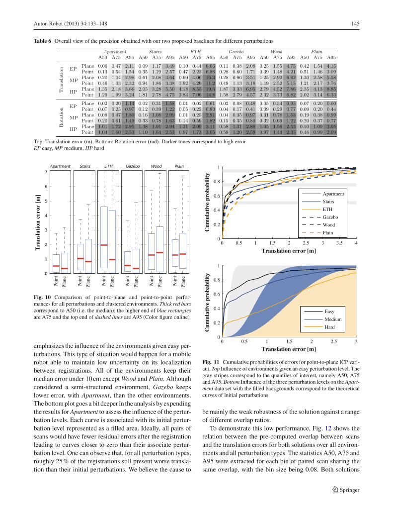
To explore the influence of the environment, Fig. 10 com-pares the translation error combining all perturbations foreach solution. Note that the A95 values for ETH exceedthe graph, being 12.16 m for point-to-point and 16.87 mfor point-to-plane. Focusing on A50 and A75, we see thatthe gain of point-to-plane over point-to-point is overcomein the data sets Wood and Plain. This observation proposesthat the accuracy of each solution follows the level of struc-ture found in each data set. When looking at the A95 statis-tics, point-to-plane is in all cases higher than point-to-point,meaning that point-to-plane does not guarantee better worst-case errors than point-to-point. It is worth noting that ETHconsists of a long hallway with repetitive elements, whichseems to drag down the A95 performance in translation whilekeeping reasonably low rotation errors (see Table 6). The dataset Plain has an even higher deficiency in term of constraintsthan ETH, with only one major plane representing the ground.Even with this level of constraint, the registrations applied inPlain seem to diverge less than in ETH for hard conditionsrepresented by A95 statistics.

Given that point-to-plane has a better overall performance,Fig. 11 focuses exclusively on that solution and shows thecumulative probabilities of its translation error. Those curvesare similar to precision-recall graphs in that the more top-left the curve the better the algorithm performs. The top plot

123

Auton Robot (2013) 34:133–148 145

Table 6 Overall view of the precision obtained with our two proposed baselines for different perturbations

Top: Translation error (m). Bottom: Rotation error (rad). Darker tones correspond to high errorEP easy, MP medium, HP hard

Fig. 10 Comparison of point-to-plane and point-to-point perfor-mances for all perturbations and clustered environments. Thick red barscorrespond to A50 (i.e. the median); the higher end of blue rectanglesare A75 and the top end of dashed lines are A95 (Color figure online)

emphasizes the influence of the environments given easy per-turbations. This type of situation would happen for a mobilerobot able to maintain low uncertainty on its localizationbetween registrations. All of the environments keep theirmedian error under 10 cm except Wood and Plain. Althoughconsidered a semi-structured environment, Gazebo keepslower error, with Apartment, than the other environments.The bottom plot goes a bit deeper in the analysis by expendingthe results for Apartment to assess the influence of the pertur-bation levels. Each curve is associated with its initial pertur-bation level represented as a filled area. Ideally, all pairs ofscans would have fewer residual errors after the registrationleading to curves closer to zero than their associate pertur-bation level. One can observe that, for all perturbation types,roughly 25 % of the registrations still present worse transla-tion than their initial perturbations. We believe the cause to

0 0.5 1 1.5 2 2.5 3 3.5 40

0.2

0.4

0.6

0.8

1

Translation error [m]

Cum

ulat

ive

prob

abili

ty

Apartment

Stairs

ETH

Gazebo

Wood

Plain

0 0.5 1 1.5 2 2.5 30

0.2

0.4

0.6

0.8

1

Translation error [m]

Cum

ulat

ive

prob

abili

ty

Easy

Medium

Hard

Fig. 11 Cumulative probabilities of errors for point-to-plane ICP vari-ant. Top Influence of environments given an easy perturbation level. Thegray stripes correspond to the quantiles of interest, namely A50, A75and A95. Bottom Influence of the three perturbation levels on the Apart-ment data set with the filled backgrounds correspond to the theoreticalcurves of initial perturbations

be mainly the weak robustness of the solution against a rangeof different overlap ratios.

To demonstrate this low performance, Fig. 12 shows therelation between the pre-computed overlap between scansand the translation errors for both solutions over all environ-ments and all perturbation types. The statistics A50, A75 andA95 were extracted for each bin of paired scan sharing thesame overlap, with the bin size being 0.08. Both solutions

123

146 Auton Robot (2013) 34:133–148

0.4 0.5 0.6 0.7 0.8 0.90

2

4

6

8

10

12

Overlap between point clouds

Tra

nsla

tion

err

or [

m]

Plane − A50

Plane − A75

Plane − A95

Point − A50

Point − A75

Point − A95

Fig. 12 Correlation between the overlap of two scans and the transla-tion error for point-to-plane over all environments and all perturbationtypes

0 1 2 3 4 5 6 7 80

0.2

0.4

0.6

0.8

1

Time per registration [s]

Cum

ulat

ive

prob

abili

ty

Apartment

Stairs

ETH

Gazebo

Wood

Plain

Fig. 13 Cumulative probabilities of the time needed to converge forpoint-to-plane with easy perturbations. The solid lines represent struc-tured environments while dashed lines represent unstructured and semi-structured environments

share the same Outlier Filtering Module tuned to handle 70and 75 % of outliers. This results in both solutions followingthe same trend leading to poor performance at low overlapvalues. The error reaches a median error larger than 2 m fora range of overlap from 0.30 to 0.38.

Finally, Fig. 13 shows the cumulative probabilities ofthe time needed to converge for point-to-plane. The figureopposes structured environments (solid lines) to unstruc-tured and semi-structured environments (dashed lines). Itis interesting to note that in Plain the solutions convergerapidly but, based on Table 6, to a large translation error.This means that the observed errors were estimated to bebelow 1 cm and 0.001 rad (see the line Transformation check-ing in Table 5) leading to an early exit out of the iterationloop. For the overall performance between the two solu-tions, point-to-point is 80 % faster than point-to-plane with amedian time of 1.45 s compared to 2.58 s respectively. Thissuggests that for point-to-plane, the extra time required toextract surface normal vectors is not compensated for by thesaving on the number of iterations required to converge. Allthe results were obtained on a 2.2 GHz Intel Core i7, usinglibpointmatcher (C++) with separate registrations run-

ning on a single core without GPU acceleration. The solutionsare not multi-threaded but we executed four tests in parallelon a single machine to reduce the total testing time.

6 Discussion

We have sub-sampled the point clouds using a fixed reduc-tion percentage leading to the use of approximately 10,000points per scan. However, the different data sets have a dif-ferent number of points per scan in average, for instanceApartment has twice as much as Stairs. It would be better toreduce the point clouds to a fixed number of points insteadof a ratio to ensure more constant processing time given thatthe precision gain is very low for a larger number of points(Pomerleau et al. 2012). As demonstrated in Fig. 8, over-lap between scans can largely vary depending on the motionof the robot and the environment configuration. One of thelimitation of trimming outliers based on quartile is that thisassumes a constant overlap of scans, which is hard to controlwith a mobile platform. In order to work around this limita-tion, it would be important to detect those places and reactappropriately. For example, the robot could acquire scansmore frequently or reduce its velocity at those places. Also,more flexible outlier-rejection algorithms need to be investi-gated to cope with the variability of the overlap.

The use of the A95 statistic might seem excessive, but itis important to note that it implies that one registration over20 is beyond this value. In the robotics context, this is verysignificant and can be the difference between a stable systemand a system that breaks its map every so often.

The point-to-plane solution can be stable for applicationswhere: first, the environment type can be controlled to behighly structured; second, the overlap is kept high while therobot is moving and third, the state estimation used as initialpose for the registration remains within 10 cm and 10◦. Thesetypes of conditions are usual for laboratory experiments butare unlikely to happen in real applications.

The procedure we propose relies on some specific data setsin order to have a common ground of comparison in the sci-entific community. However, as the sensor is the same acrossall data sets, we cannot measure its effect on the ICP per-formances. The sensor has nevertheless two important fea-tures, noise and field of view, that can have an influence onICP. Indeed, sensors may have different noise levels and evennoise profiles, and different ICP variants might cope betterwith some than others. Furthermore, the field of view and thepoint-density profile of the sensor inside its field of view canhave a huge influence on the ICP performance as those char-acteristics govern the overlap and the possibility of multiplepairings between scans.

Finally, as explained previously, some applications requireonline matching of sensor data. In these cases, the time spent

123

Auton Robot (2013) 34:133–148 147

in ICP is a relevant criterion to compare variants. However,processing time is difficult to measure given that internalmemory management, processor load and processor types areall relevant factors that cannot easily be compensated for andthat can drastically change time measurements. On the otherhand, theoretical complexity is not sufficient as different ICPvariants will mostly have a comparable complexity but dif-ferent constant factors. Having a single computer dedicatedto running all the different ICP variants in the same conditionwould yield a general idea of the relative efficiency. However,different ICP variants would scale differently for differentpractical cases. A comparison of the variants in the specificcase of application is thus always pertinent. Our library canfacilitate this comparison by highlighting only the relevantchanges. Indeed, the efficiency of an implementation is animportant factor of time performance that can bias the com-parison of algorithms. Having a library in which only themodules to be compared change already significantly reducesthis effect by maintaining a homogeneous environment formost data processing.

In a nutshell, researchers using our protocol should main-tain a certain uniformity by:

1. Characterizing the main parameters of their novel solu-tion.

2. Evaluating their solutions using the predefined data setsand pairs of scans and perturbations.

3. Recording translation and rotation errors following Eqs. 2and 3.

4. Recording computational time excluding data acquisitionbut including preprocessing steps.

5. Reporting strength and weakness against environmenttype, perturbation level and overlap ratio.

6. Comparing their results with formal solution in terms ofprecision and accuracy using A50, A75 and A95 statis-tics.

7. Making their results publicly available, when possible,so that other researchers can accelerate the comparisonprocess.

7 Conclusion

In this paper, we proposed a protocol to compare ICP vari-ants. We lay the emphasis on the repeatability of the resultsby selecting publicly available data sets. We also presented anopen-source modular ICP library that can further improve onthe repeatability by allowing easy tests and comparisons withbaseline variants. Thus, this modular library is the companionof choice of our protocol. Finally, we demonstrated our evalu-ation framework by comparing well-established ICP variantsin a rich variety of environments. This refreshes the obser-vations from Rusinkiewicz and Levoy (2001) by using data

sets closer to robotic applications. The performances of thesebaseline variants show a high variability and strongly displaythe need for improved ICP methods for natural, unstructuredand information-deprived environments. This need opens thedoor for other researchers to challenge their novel solutionsagainst our baselines.

We would welcome additional data sets with different sen-sors and other ICP implementations, but our comparison isalready a stepping stone in ICP comparison that can be builtupon. We believe that this combination of protocol, softwareand baseline results shows nicely how open-source softwarecan drive research forward.

Acknowledgments This work was supported by the EU FP7 IPprojects Natural Human-Robot Cooperation in Dynamic Environments(ICT-247870) and myCopter (FP7-AAT-2010-RTD-1). F. Pomerleauwas supported by a fellowship from the Fonds québécois de recherchesur la nature et les technologies (FQRNT).

References

Amigoni, F., Reggiani, M., & Schiaffonati, V. (2009). An insightfulcomparison between experiments in mobile robotics and in science.Autonomous Robots, 27(4), 313–325.

Armesto, L., Minguez, J., & Montesano, L. (2010). A generalizationof the metric-based iterative closest point technique for 3D scanmatching. In Proceedings of the IEEE international conference onrobotics and automation (pp. 1367–1372).

Arya, S., & Mount, D. (1993). Approximate nearest neighbor queriesin fixed dimensions. In Proceedings of the 4th annual ACM-SIAMsymposium on discrete algorithms (pp. 271–280).

Baker, S., Scharstein, D., Lewis, J., Roth, S., Black, M., & Szeliski,R. (2007). A database and evaluation methodology for optical flow.International Journal of Computer Vision, 92, 1–31.

Ben-Kiki, O., Evans, C., & Ingerson, B. (2009). YAML ain’t markuplanguage (YAMLTM) version 1.2. http://www.yaml.org/spec/1.2/spec.html.

Besl, P., & McKay, H. (1992). A method for registration of 3-D shapes.IEEE Transactions on Pattern Analysis and Machine Intelligence,14(2), 239–256.

Chen, Y., & Medioni, G. (1991). Object modeling by registration ofmultiple range images. In Proceedings of the IEEE internationalconference on robotics and automation (pp. 2724–2729). New York:IEEE Computer Society Press.

Chetverikov, D., Svirko, D., Stepanov, D., & Krsek, P. (2002). Thetrimmed iterative closest point algorithm. In Proceedings of the 16thinternational conference on pattern recognition (pp. 545–548).

Elseberg, J., Magnenat, S., Siegwart, R., & Nüchter, A. (2012). Com-parison of nearest-neighbor-search strategies and implementationsfor efficient shape registration. Journal of Software Engineering forRobotics, 3(1), 2–12.

Geiger, A., Lenz, P., & Urtasun, R. (2012). Are we ready for autonomousdriving? The KITTI vision benchmark suite. In Computer vision andpattern recognition (CVPR).

Hugli, H., & Schutz, C. (1997). Geometric matching of 3D objects:Assessing the range of successful initial configurations. In Proceed-ings of the international conference on recent advances in 3-D digitalimaging and modeling (pp. 101–106).

Huynh, D. Q. (2009). Metrics for 3D rotations: Comparison and analy-sis. Journal of Mathematical Imaging and Vision, 35(2), 155–164.

123

148 Auton Robot (2013) 34:133–148

Jian, B., & Vemuri, B. C. (2011). Robust point set registration usingGaussian mixture models. IEEE Transactions on Pattern Analysisand Machine Intelligence, 33(8), 1633–1645.

Magnusson, M., Lilienthal, A., & Duckett, T. (2007). Scan registrationfor autonomous mining vehicles using 3D-NDT. Journal of FieldRobotics, 24(10), 803–827.

Magnusson, M., Nüchter, A., Lorken, C., Lilienthal, A., & Hertzberg, J.(2009). Evaluation of 3D registration reliability and speed—A com-parison of ICP and NDT. In Proceedings of the IEEE internationalconference on robotics and automation (pp. 3907–3912).

May, S., Droeschel, D., Holz, D., Fuchs, S., Malis, E., Nüchter, A.,Hertzberg, J. (2009). Three-dimensional mapping with time-of-flightcameras. Journal of Field Robotics, 26(11–12), 934–965.

Pathak, K., Borrmann, D., Elseberg, J., Vaskevicius, N., Birk, A., &Nüchter, A. (2010). Evaluation of the robustness of planar-patchesbased 3D-registration using marker-based ground-truth in an out-door urban scenario. In Proceedings of the IEEE/RSJ internationalconference on intelligent robots and systems (pp. 5725–5730).

Pomerleau, F., Liu, M., Colas, F., & Siegwart, R. (2012). Challengingdata sets for point cloud registration algorithms. The InternationalJournal of Robotics Research.

Pomerleau, F., Magnenat, S., Colas, F., Liu, M., & Siegwart, R. (2011)Tracking a depth camera: Parameter exploration for fast ICP. In Pro-ceedings of the IEEE/RSJ international conference on intelligentrobots and systems (pp. 3824–3829).

Rusinkiewicz, S., & Levoy, M. (2001). Efficient variants of the ICPalgorithm. In Proceedings of the third international conference on3-D digital imaging and modeling (pp. 145–152).

Rusu, R., & Cousins, S. (2011). 3D is here: Point cloud library (PCL).In Proceedings of the IEEE international conference on robotics andautomation (pp. 1–4).

Scharstein, D., & Szeliski, R. (2002). A taxonomy and evaluation ofdense two-frame stereo correspondence algorithms. InternationalJournal of Computer Vision, 47(1), 7–42.

Schroeder, W., Martin, K., & Lorensen, B. (2006). Visualization toolkit:An object-oriented approach to 3D graphics (4th ed.). Clifton Park,NY: Kitware.

Seitz, S. M., Curless, B., Diebel, J., Scharstein, D., & Szeliski, R. (2006).A comparison and evaluation of multi-view stereo reconstructionalgorithms. In Proceedings of the IEEE computer society conferenceon computer vision and pattern recognition (pp. 519–528).

Tong, C. H., Barfoot, T. D., & Dupuis, É. (2012). Three-dimensionalSLAM for mapping planetary work site environments. Journal ofField Robotics, 29, 381–412.

Wulf, O., Nüchter, A., Hertzberg, J., & Wagner, B. (2008). Bench-marking urban six-degree-of-freedom simultaneous localization andmapping. Journal of Field Robotics, 25(3), 148–163.

Author Biographies

François Pomerleau is a PhDstudent at the Autonomous Sys-tems Lab in ETH Zurich. Hereceived M.Sc. degree from Uni-versité de Sherbrooke, Canadain 2009. His research interestsinclude 3D localization and map-ping, registration algorithms andfield robotics aiming at bringrobots outside research laborato-ries.

Francis Colas is a postdoctoralfellow at the Autonomous Sys-tems Lab. (ETH Zurich) sinceJanuary 2009. He received aPh.D. degree in Computer Sci-ence from the INPG, in 2006.Subsequently, he joined the Col-lege de France, Paris, Franceas a Postdoctoral Fellow in theLaboratoire de Physiologie de laPerception et de l’Action, from2007 to 2008. In January 2009,he joined the Autonomous Sys-tems Lab. His research interestsinclude Bayesian modeling of

perception and action applied from cognitive sciences to robotics.

Roland Siegwart is a full pro-fessor for Autonomous Systemsand Vice President Researchand Corporate Relations at ETHZurich since 2006 and 2010respectively. From 1996 to 2006he was associate and later fullprofessor for Autonomous Micro-systems and Robots at the EcolePolytechnique Fédérale de Lau-sanne (EPFL). Roland Siegwartis member of the Swiss Academyof Engineering Sciences, IEEEFellow and officer of the Inter-national Federation of Robotics

Research (IFRR). He served as Vice President for Technical Activities(2004/2005) and was awarded Distinguished Lecturer (2006/2007) andis currently an AdCom Member (2007–2010) of the IEEE Robotics andAutomation Society. He leads a research group of around 30 peopleworking in the fields of robotics, mechatronics and product design.

Stéphane Magnenat is seniorresearcher at the AutonomousSystems Lab in ETH Zurich.He received the M.Sc. degreein computer science (2003) andthe Ph.D. degree (2010) fromÉcole Polytechnique Fédérale deLausanne (EPFL). His researchinterests include software archi-tecture, software integration andscalable artificial intelligence onmobile robots. He is enthusiasticabout open source software as amean to advance mobile roboticsand its adoption. He is a memberof the IEEE.

123