Comparing Fault Resistance Coverage of Different Distribution System

Grounding Methods

Daqing Hou Schweitzer Engineering Laboratories, Inc.

Revised edition released October 2010

Originally presented at the 37th Annual Western Protective Relay Conference, October 2010

1

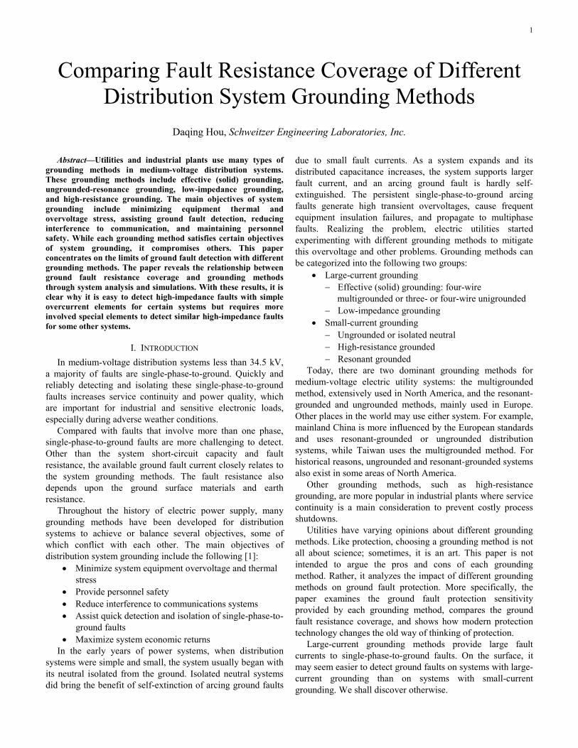
Comparing Fault Resistance Coverage of Different Distribution System Grounding Methods

Daqing Hou, Schweitzer Engineering Laboratories, Inc.

Abstract—Utilities and industrial plants use many types of grounding methods in medium-voltage distribution systems. These grounding methods include effective (solid) grounding, ungrounded-resonance grounding, low-impedance grounding, and high-resistance grounding. The main objectives of system grounding include minimizing equipment thermal and overvoltage stress, assisting ground fault detection, reducing interference to communication, and maintaining personnel safety. While each grounding method satisfies certain objectives of system grounding, it compromises others. This paper concentrates on the limits of ground fault detection with different grounding methods. The paper reveals the relationship between ground fault resistance coverage and grounding methods through system analysis and simulations. With these results, it is clear why it is easy to detect high-impedance faults with simple overcurrent elements for certain systems but requires more involved special elements to detect similar high-impedance faults for some other systems.

I. INTRODUCTION In medium-voltage distribution systems less than 34.5 kV,

a majority of faults are single-phase-to-ground. Quickly and reliably detecting and isolating these single-phase-to-ground faults increases service continuity and power quality, which are important for industrial and sensitive electronic loads, especially during adverse weather conditions.

Compared with faults that involve more than one phase, single-phase-to-ground faults are more challenging to detect. Other than the system short-circuit capacity and fault resistance, the available ground fault current closely relates to the system grounding methods. The fault resistance also depends upon the ground surface materials and earth resistance.

Throughout the history of electric power supply, many grounding methods have been developed for distribution systems to achieve or balance several objectives, some of which conflict with each other. The main objectives of distribution system grounding include the following [1]:

• Minimize system equipment overvoltage and thermal stress

• Provide personnel safety • Reduce interference to communications systems • Assist quick detection and isolation of single-phase-to-

ground faults • Maximize system economic returns

In the early years of power systems, when distribution systems were simple and small, the system usually began with its neutral isolated from the ground. Isolated neutral systems did bring the benefit of self-extinction of arcing ground faults

due to small fault currents. As a system expands and its distributed capacitance increases, the system supports larger fault current, and an arcing ground fault is hardly self-extinguished. The persistent single-phase-to-ground arcing faults generate high transient overvoltages, cause frequent equipment insulation failures, and propagate to multiphase faults. Realizing the problem, electric utilities started experimenting with different grounding methods to mitigate this overvoltage and other problems. Grounding methods can be categorized into the following two groups:

• Large-current grounding − Effective (solid) grounding: four-wire

multigrounded or three- or four-wire unigrounded − Low-impedance grounding

• Small-current grounding − Ungrounded or isolated neutral − High-resistance grounded − Resonant grounded

Today, there are two dominant grounding methods for medium-voltage electric utility systems: the multigrounded method, extensively used in North America, and the resonant-grounded and ungrounded methods, mainly used in Europe. Other places in the world may use either system. For example, mainland China is more influenced by the European standards and uses resonant-grounded or ungrounded distribution systems, while Taiwan uses the multigrounded method. For historical reasons, ungrounded and resonant-grounded systems also exist in some areas of North America.

Other grounding methods, such as high-resistance grounding, are more popular in industrial plants where service continuity is a main consideration to prevent costly process shutdowns.

Utilities have varying opinions about different grounding methods. Like protection, choosing a grounding method is not all about science; sometimes, it is an art. This paper is not intended to argue the pros and cons of each grounding method. Rather, it analyzes the impact of different grounding methods on ground fault protection. More specifically, the paper examines the ground fault protection sensitivity provided by each grounding method, compares the ground fault resistance coverage, and shows how modern protection technology changes the old way of thinking of protection.

Large-current grounding methods provide large fault currents to single-phase-to-ground faults. On the surface, it may seem easier to detect ground faults on systems with large-current grounding than on systems with small-current grounding. We shall discover otherwise.

2

This paper devotes a section to each grounding method, briefly points out the main benefits and shortcomings of each method, and discusses the ground fault detection characteristics provided by the grounding method. More attention is devoted to the ungrounded and multigrounded distribution systems because they are more representative of each grounding category.

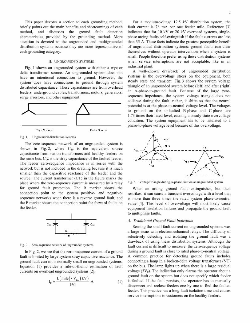
II. UNGROUNDED SYSTEMS Fig. 1 shows an ungrounded system with either a wye or

delta transformer source. An ungrounded system does not have an intentional connection to ground. However, the system does have connections to ground through system distributed capacitance. These capacitances are from overhead feeders, underground cables, transformers, motors, generators, surge arrestors, and other equipment.

Fig. 1. Ungrounded distribution systems

The zero-sequence network of an ungrounded system is shown in Fig. 2, where CS0 is the equivalent source capacitance from station transformers and healthy feeders on the same bus. CL0 is the stray capacitance of the faulted feeder. The feeder zero-sequence impedance is in series with the network but is not included in the drawing because it is much smaller than the capacitive reactance of the feeder and the source. The current transformer (CT) in the figure marks the place where the zero-sequence current is measured by a relay for ground fault protection. The R marker shows the connection point to the system positive- and negative-sequence networks when there is a reverse ground fault, and the F marker shows the connection point for forward faults on the feeder.

CS0 CL0

R F

Fig. 2. Zero-sequence network of ungrounded systems

In Fig. 2, we see that the zero-sequence current of a ground fault is limited by large system stray capacitive reactance. The ground fault current is normally small on ungrounded systems. Equation (1) provides a rule-of-thumb estimation of fault currents on overhead ungrounded systems [2].

( ) ( )LL

FL mile • V kV

I A160

= (1)

For a medium-voltage 12.5 kV distribution system, the fault current is 78 mA per one feeder mile. Reference [3] indicates that for 10 kV or 20 kV overhead systems, single-phase arcing faults self-extinguish if the fault currents are less than 35 A. These facts indicate the greatest perceptible benefit of ungrounded distribution systems: ground faults can clear themselves without operator intervention when a system is small. People therefore prefer using these distribution systems when service interruptions are not acceptable, like in an industrial plant.

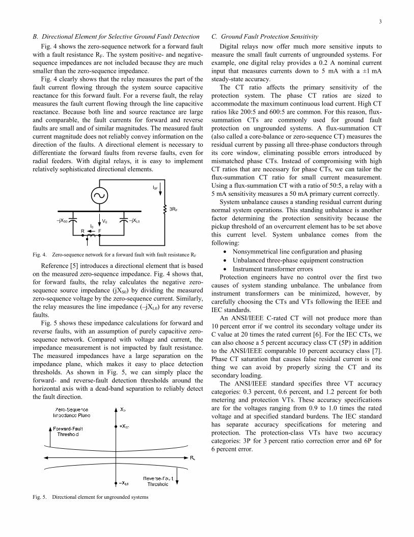
A well-known drawback of ungrounded distribution systems is the overvoltage stress on the equipment, both steady state and transient. Fig. 3 shows the system voltage triangle of an ungrounded system before (left) and after (right) an A-phase-to-ground fault. Because of the large zero-sequence impedance, the system voltage triangle does not collapse during the fault; rather, it shifts so that the neutral potential is at the phase-to-neutral voltage level. The voltages to ground on the unfaulted B-phase and C-phase are 1.73 times their rated level, causing a steady-state overvoltage condition. The system equipment has to be insulated to a phase-to-phase voltage level because of this overvoltage.

Fig. 3. Voltage triangle during A-phase fault on an ungrounded system

When an arcing ground fault extinguishes, but then restrikes, it can cause a transient overvoltage with a level that is more than three times the rated system phase-to-neutral value [4]. This level of overvoltage will most likely cause equipment insulation failures and propagate the ground fault to multiphase faults.

A. Traditional Ground Fault Indication Sensing the small fault current on ungrounded systems was

a large issue with electromechanical relays. The difficulty of selectively detecting and isolating the ground fault was a drawback of using these distribution systems. Although the fault current is difficult to measure, the zero-sequence voltage during a ground fault is close to rated phase-to-neutral voltage. A common practice for detecting ground faults includes connecting a lamp in a broken-delta voltage transformer (VT) on the bus. The lamp lights up when there is a large residual voltage (3V0). The indication only alarms the operator about a ground fault on the system but does not specify which feeder is faulted. If the fault persists, the operator has to manually disconnect and reclose feeders one by one to find the faulted feeder. This practice has a long fault isolation time and causes service interruptions to customers on the healthy feeders.

3

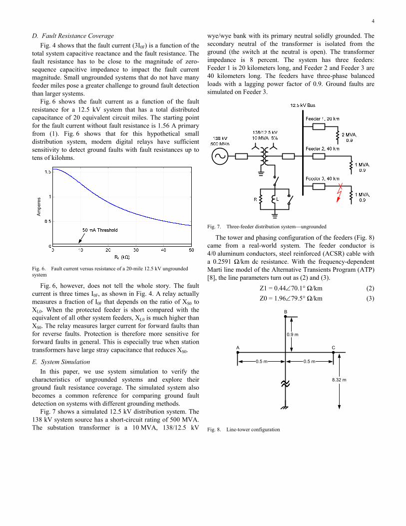
B. Directional Element for Selective Ground Fault Detection Fig. 4 shows the zero-sequence network for a forward fault

with a fault resistance RF. The system positive- and negative-sequence impedances are not included because they are much smaller than the zero-sequence impedance.

Fig. 4 clearly shows that the relay measures the part of the fault current flowing through the system source capacitive reactance for this forward fault. For a reverse fault, the relay measures the fault current flowing through the line capacitive reactance. Because both line and source reactance are large and comparable, the fault currents for forward and reverse faults are small and of similar magnitudes. The measured fault current magnitude does not reliably convey information on the direction of the faults. A directional element is necessary to differentiate the forward faults from reverse faults, even for radial feeders. With digital relays, it is easy to implement relatively sophisticated directional elements.

–jXS0

R F

–jXL0V0I0

I0F

3RF

Fig. 4. Zero-sequence network for a forward fault with fault resistance RF

Reference [5] introduces a directional element that is based on the measured zero-sequence impedance. Fig. 4 shows that, for forward faults, the relay calculates the negative zero-sequence source impedance (jXS0) by dividing the measured zero-sequence voltage by the zero-sequence current. Similarly, the relay measures the line impedance (–jXL0) for any reverse faults.

Fig. 5 shows these impedance calculations for forward and reverse faults, with an assumption of purely capacitive zero-sequence network. Compared with voltage and current, the impedance measurement is not impacted by fault resistance. The measured impedances have a large separation on the impedance plane, which makes it easy to place detection thresholds. As shown in Fig. 5, we can simply place the forward- and reverse-fault detection thresholds around the horizontal axis with a dead-band separation to reliably detect the fault direction.

Fig. 5. Directional element for ungrounded systems

C. Ground Fault Protection Sensitivity Digital relays now offer much more sensitive inputs to

measure the small fault currents of ungrounded systems. For example, one digital relay provides a 0.2 A nominal current input that measures currents down to 5 mA with a ±1 mA steady-state accuracy.

The CT ratio affects the primary sensitivity of the protection system. The phase CT ratios are sized to accommodate the maximum continuous load current. High CT ratios like 200:5 and 600:5 are common. For this reason, flux-summation CTs are commonly used for ground fault protection on ungrounded systems. A flux-summation CT (also called a core-balance or zero-sequence CT) measures the residual current by passing all three-phase conductors through its core window, eliminating possible errors introduced by mismatched phase CTs. Instead of compromising with high CT ratios that are necessary for phase CTs, we can tailor the flux-summation CT ratio for small current measurement. Using a flux-summation CT with a ratio of 50:5, a relay with a 5 mA sensitivity measures a 50 mA primary current correctly.

System unbalance causes a standing residual current during normal system operations. This standing unbalance is another factor determining the protection sensitivity because the pickup threshold of an overcurrent element has to be set above this current level. System unbalance comes from the following:

• Nonsymmetrical line configuration and phasing • Unbalanced three-phase equipment construction • Instrument transformer errors

Protection engineers have no control over the first two causes of system standing unbalance. The unbalance from instrument transformers can be minimized, however, by carefully choosing the CTs and VTs following the IEEE and IEC standards.

An ANSI/IEEE C-rated CT will not produce more than 10 percent error if we control its secondary voltage under its C value at 20 times the rated current [6]. For the IEC CTs, we can also choose a 5 percent accuracy class CT (5P) in addition to the ANSI/IEEE comparable 10 percent accuracy class [7]. Phase CT saturation that causes false residual current is one thing we can avoid by properly sizing the CT and its secondary loading.

The ANSI/IEEE standard specifies three VT accuracy categories: 0.3 percent, 0.6 percent, and 1.2 percent for both metering and protection VTs. These accuracy specifications are for the voltages ranging from 0.9 to 1.0 times the rated voltage and at specified standard burdens. The IEC standard has separate accuracy specifications for metering and protection. The protection-class VTs have two accuracy categories: 3P for 3 percent ratio correction error and 6P for 6 percent error.

4

D. Fault Resistance Coverage Fig. 4 shows that the fault current (3I0F) is a function of the

total system capacitive reactance and the fault resistance. The fault resistance has to be close to the magnitude of zero-sequence capacitive impedance to impact the fault current magnitude. Small ungrounded systems that do not have many feeder miles pose a greater challenge to ground fault detection than larger systems.

Fig. 6 shows the fault current as a function of the fault resistance for a 12.5 kV system that has a total distributed capacitance of 20 equivalent circuit miles. The starting point for the fault current without fault resistance is 1.56 A primary from (1). Fig. 6 shows that for this hypothetical small distribution system, modern digital relays have sufficient sensitivity to detect ground faults with fault resistances up to tens of kilohms.

Am

pere

s

Fig. 6. Fault current versus resistance of a 20-mile 12.5 kV ungrounded system

Fig. 6, however, does not tell the whole story. The fault current is three times I0F, as shown in Fig. 4. A relay actually measures a fraction of I0F that depends on the ratio of XS0 to XL0. When the protected feeder is short compared with the equivalent of all other system feeders, XL0 is much higher than XS0. The relay measures larger current for forward faults than for reverse faults. Protection is therefore more sensitive for forward faults in general. This is especially true when station transformers have large stray capacitance that reduces XS0.

E. System Simulation In this paper, we use system simulation to verify the

characteristics of ungrounded systems and explore their ground fault resistance coverage. The simulated system also becomes a common reference for comparing ground fault detection on systems with different grounding methods.

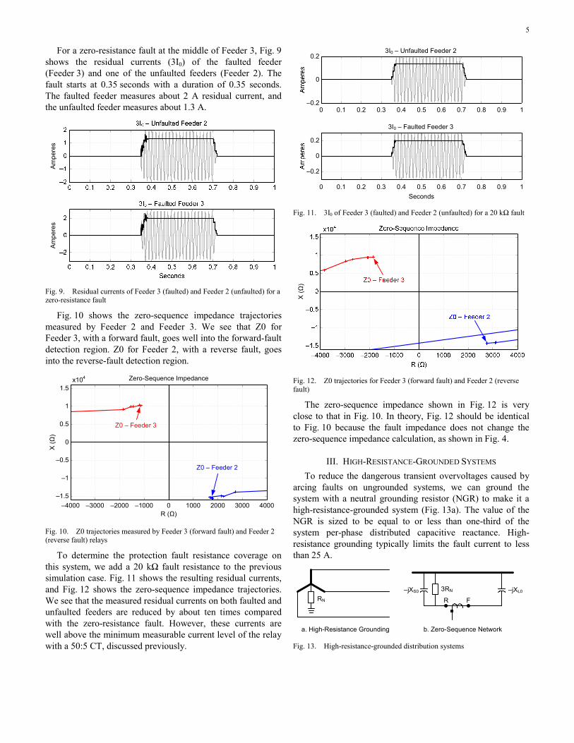
Fig. 7 shows a simulated 12.5 kV distribution system. The 138 kV system source has a short-circuit rating of 500 MVA. The substation transformer is a 10 MVA, 138/12.5 kV

wye/wye bank with its primary neutral solidly grounded. The secondary neutral of the transformer is isolated from the ground (the switch at the neutral is open). The transformer impedance is 8 percent. The system has three feeders: Feeder 1 is 20 kilometers long, and Feeder 2 and Feeder 3 are 40 kilometers long. The feeders have three-phase balanced loads with a lagging power factor of 0.9. Ground faults are simulated on Feeder 3.

Fig. 7. Three-feeder distribution system—ungrounded

The tower and phasing configuration of the feeders (Fig. 8) came from a real-world system. The feeder conductor is 4/0 aluminum conductors, steel reinforced (ACSR) cable with a 0.2591 Ω/km dc resistance. With the frequency-dependent Marti line model of the Alternative Transients Program (ATP) [8], the line parameters turn out as (2) and (3). Z1 = 0.44∠70.1° Ω/km (2) Z0 = 1.96∠79.5° Ω/km (3)

A

B

C

0.5 m0.5 m

0.9 m

8.32 m

Fig. 8. Line-tower configuration

5

For a zero-resistance fault at the middle of Feeder 3, Fig. 9 shows the residual currents (3I0) of the faulted feeder (Feeder 3) and one of the unfaulted feeders (Feeder 2). The fault starts at 0.35 seconds with a duration of 0.35 seconds. The faulted feeder measures about 2 A residual current, and the unfaulted feeder measures about 1.3 A.

Am

pere

sA

mpe

res

Fig. 9. Residual currents of Feeder 3 (faulted) and Feeder 2 (unfaulted) for a zero-resistance fault

Fig. 10 shows the zero-sequence impedance trajectories measured by Feeder 2 and Feeder 3. We see that Z0 for Feeder 3, with a forward fault, goes well into the forward-fault detection region. Z0 for Feeder 2, with a reverse fault, goes into the reverse-fault detection region.

Zero-Sequence Impedancex104

1.5

1

0.5

0

–0.5

–1

–1.5

X (Ω

)

R (Ω)–4000 –3000 –2000 –1000 0 1000 2000 3000 4000

Z0 – Feeder 3

Z0 – Feeder 2

Fig. 10. Z0 trajectories measured by Feeder 3 (forward fault) and Feeder 2 (reverse fault) relays

To determine the protection fault resistance coverage on this system, we add a 20 kΩ fault resistance to the previous simulation case. Fig. 11 shows the resulting residual currents, and Fig. 12 shows the zero-sequence impedance trajectories. We see that the measured residual currents on both faulted and unfaulted feeders are reduced by about ten times compared with the zero-resistance fault. However, these currents are well above the minimum measurable current level of the relay with a 50:5 CT, discussed previously.

3I0 – Unfaulted Feeder 20.2

0

–0.20 0.1 0.2 0.3 0.4 0.5 0.6 0.7 0.8 0.9 1

0.2

0

–0.2

3I0 – Faulted Feeder 3

0 0.1 0.2 0.3 0.4 0.5 0.6 0.7 0.8 0.9 1Seconds

Fig. 11. 3I0 of Feeder 3 (faulted) and Feeder 2 (unfaulted) for a 20 kΩ fault

X (Ω

)

Fig. 12. Z0 trajectories for Feeder 3 (forward fault) and Feeder 2 (reverse fault)

The zero-sequence impedance shown in Fig. 12 is very close to that in Fig. 10. In theory, Fig. 12 should be identical to Fig. 10 because the fault impedance does not change the zero-sequence impedance calculation, as shown in Fig. 4.

III. HIGH-RESISTANCE-GROUNDED SYSTEMS To reduce the dangerous transient overvoltages caused by

arcing faults on ungrounded systems, we can ground the system with a neutral grounding resistor (NGR) to make it a high-resistance-grounded system (Fig. 13a). The value of the NGR is sized to be equal to or less than one-third of the system per-phase distributed capacitive reactance. High-resistance grounding typically limits the fault current to less than 25 A.

3RN –jXL0–jXS0

R FRN

a. High-Resistance Grounding b. Zero-Sequence Network

Fig. 13. High-resistance-grounded distribution systems

6

Fig. 13b shows the zero-sequence network of a high-resistance-grounded system. The figure does not include the transformer and system zero-sequence impedances that are in series with the NGR because their values are much smaller than the NGR. The line zero-sequence impedance is also not included because of its much smaller value compared with the distributed line capacitive reactance.

Because of their small fault currents, high-resistance-grounded systems are quite similar to ungrounded systems, in terms of ground fault detection. Detecting the faulted feeder requires a directional element. Fig. 13b shows that the source impedance measured by a relay for forward faults is equal to 3RN and jXS0 in parallel. When 3RN = (XS0 + XL0) and XL0<<XS0, this source impedance angle is close to 135 degrees. We can adjust the maximum torque angle of the Fig. 5 directional element to increase the fault detection sensitivity for high-resistance-grounded systems [9]. Fig. 14 shows this maximum torque angle adjustment.

–jXL0

X0

R0

Z0MTA

3RN – jXS0

Forward Faults

Reverse Faults

j3RNXS0

Fig. 14. Directional element for high-resistance-grounded systems

Because the NGR increases the fault current by about 1.41 times, the ground fault detection sensitivity for high-resistance-grounded systems is higher than that for ungrounded systems. The fault resistance coverage is well into tens of kilohms.

IV. RESONANT-GROUNDED SYSTEMS When an ungrounded system contains many feeder miles,

the resulting system stray capacitance may be so large that arcing ground faults cannot self-extinguish. By grounding the system neutral using an inductor, we can compensate the capacitive fault current. In the 100 percent compensation condition (when the inductive reactance is equal to one-third of the system zero-sequence capacitive reactance), the system achieves parallel resonance. The ground fault current is normally under a few amperes on resonant-grounded systems.

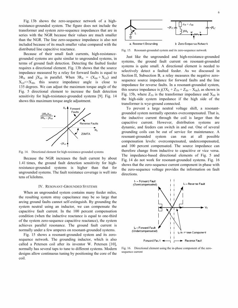
Fig. 15 shows a resonant-grounded system and its zero-sequence network. The grounding inductor, which is also called a Petersen coil after its inventor W. Petersen [10], normally has several taps to tune to different systems. Modern designs allow continuous tuning by positioning the core of the coil.

Fig. 15. Resonant-grounded system and its zero-sequence network

Just like the ungrounded and high-resistance-grounded systems, the ground fault current on resonant-grounded systems is quite small. A directional element is needed to selectively detect a faulted feeder. As we discussed in Section II, Subsection B, a relay measures the negative zero-sequence source impedance for forward faults and the line impedance for reverse faults. In a resonant-grounded system, this source impedance is j(3XL + ZT0 + ZS0 – XS0), as shown in Fig. 15b, where ZT0 is the transformer impedance and XS0 is the high-side system impedance if the high side of the transformer is wye-ground connected.

To prevent a large neutral voltage shift, a resonant-grounded system normally operates overcompensated. That is, the inductive current through the coil is larger than the capacitive current. However, distribution systems are dynamic, and feeders can switch in and out. One of several grounding coils can be out of service for maintenance. A resonant-grounded system can run at all possible compensation levels: overcompensated, undercompensated, and 100 percent compensated. The source impedance can therefore change from inductive to capacitive or vice versa. The impedance-based directional elements of Fig. 5 and Fig. 14 do not work for resonant-grounded systems. Fig. 16 shows that the zero-sequence current component in phase with the zero-sequence voltage provides the information on fault directions.

Fig. 16. Directional element using the in-phase component of the zero-sequence current

7

Fig. 16 exaggerates the amount of the in-phase component. In reality, this component is quite small, because it comes from the losses of the station transformer, grounding coil, and feeders. The leakage conductance for a typical overhead feeder is around 5 microsiemens (μS) per mile. We need a high CT phase angle accuracy to preserve the subtle in-phase component.

A traditional directional element for resonant-grounded systems is a wattmetric element, which has the operating characteristic represented with dash-dotted lines in Fig. 16. Using overvoltage element supervision increases the security of the wattmetric element so that it does not misoperate under normal system standing unbalance. Because the standing zero-sequence voltage can be high in resonant-grounded systems, the threshold for the overvoltage supervision is routinely set to 20 percent of the rated voltage. The voltage supervision therefore limits the sensitivity of the element for detecting high-impedance faults.

Reference [1] introduces an incremental conductance directional element. The element uses the in-phase quantity just like the wattmetric element. However, by calculating the delta change of conductance, the element does eliminate the standing unbalance from normal system operation and greatly increases the fault detection sensitivity. The simulation results in [1] show that the incremental conductance directional element easily detects faults with a fault resistance up to 80 kΩ.

V. MULTIGROUNDED SYSTEMS Fig. 17 shows a multigrounded system. The neutral wire is

grounded at the substation transformer neutral and at every end-user distribution transformer location. The neutral is grounded at no less than four points per mile if there is no distribution transformer available for grounding. The system grounding quality of multigrounded systems does not depend on the grounding condition at a single location. Therefore, multigrounded systems are normally effectively grounded. They comply with R0 ≤ X1 and X0 ≤ 3X1, where R0 and X0 are system zero-sequence resistance and reactance and X1 is system positive-sequence reactance [11].

Fig. 17. Multigrounded distribution systems

The main benefit of multigrounded systems is low steady-state and transient overvoltage. The voltage rise of unfaulted phases during a single-phase-to-ground fault is less than 25 percent for multigrounded systems [12]. The system equipment insulation can be rated at the system phase-to-neutral voltage level, and therefore, the overall system cost can be less than that for ungrounded or high-resistance-grounded systems.

System loads can be either phase-to-phase or phase-to-ground on multigrounded systems. Because of this flexibility, there are many single-phase laterals on a multigrounded system, especially in rural areas.

Because of small system zero-sequence impedance, ground fault current can be large on multigrounded systems. Ground faults require immediate isolation to reduce equipment thermal damage and ensure system integrity.

Fig. 18 shows the zero-sequence network of multigrounded systems with balanced loads, where ZS0, ZT0, ZL0, and ZLD0 are the zero-sequence impedances of the system, substation transformer, line, and load, respectively. Again, the CT in the figure marks the place where the zero-sequence current is measured for ground fault protection. The R marker is the point of connection to the system positive- and negative-sequence networks for reverse ground faults, and the F marker is the connection point for forward faults on the feeder.

Fig. 18. Zero-sequence network of multigrounded systems with balanced loads

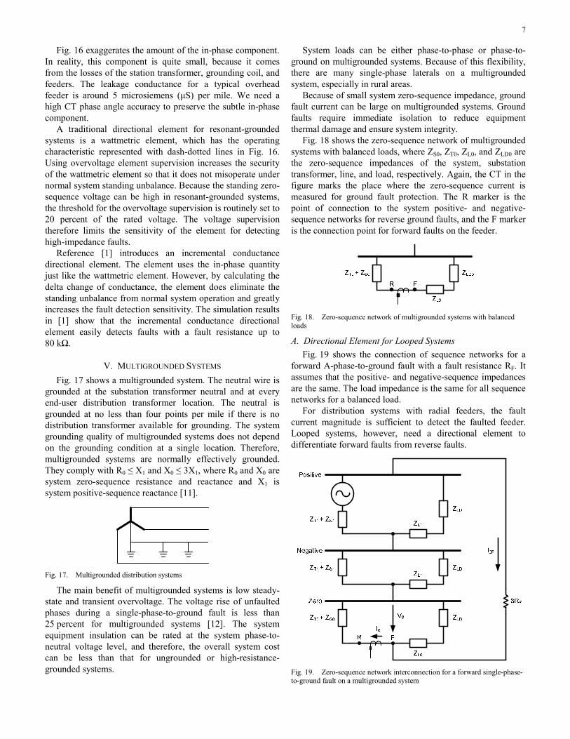
A. Directional Element for Looped Systems Fig. 19 shows the connection of sequence networks for a

forward A-phase-to-ground fault with a fault resistance RF. It assumes that the positive- and negative-sequence impedances are the same. The load impedance is the same for all sequence networks for a balanced load.

For distribution systems with radial feeders, the fault current magnitude is sufficient to detect the faulted feeder. Looped systems, however, need a directional element to differentiate forward faults from reverse faults.

Fig. 19. Zero-sequence network interconnection for a forward single-phase-to-ground fault on a multigrounded system

8

Fig. 19 shows that, for forward faults, the relay calculates the total source impedance –(ZT0 + ZS0) by dividing the measured zero-sequence voltage by the zero-sequence current. Similarly, the relay calculates the line plus load impedance (ZL0 + ZLD) for reverse faults. Using these distinctive impedance measurements for forward and reverse faults, one digital relay has a directional element with the characteristic shown in Fig. 20 [5]. This figure assumes pure inductive reactance for all impedance. The detection characteristic simply places the forward- and reverse-fault detection thresholds around one-half the distance between the impedance measured for forward and reverse faults on the vertical axis. A dead band that separates the forward- and reverse-fault detection thresholds increases the dependability and security of the directional element. Compared with the traditional torque-type directional element design, this impedance-based element does not suffer a sensitivity problem when there is a strong source behind the relay that results in a close-to-zero voltage measurement. A similar directional element based on negative-sequence quantities can be used for all faults other than three-phase faults.

Forward Faults

Reverse Faults

X0

R0–(ZS0 + ZT0)

ZL0 + ZLD

ZL0

Z0F

Z0R

Fig. 20. Directional element characteristic for multigrounded systems

B. System Unbalance Caused by Single-Phase Laterals There is a common misconception that multigrounding

provides better ground fault detection because of large available fault current. However, in multigrounded systems, the standing load unbalance is the major factor that limits the sensitivity of ground fault protection. System operation engineers may do a good job of evenly distributing single-phase loads among different phases and achieving a good balance at the substation during normal system operations. To prevent protection misoperations, protection engineers need to consider the worst system operating scenario, where a large single-phase lateral is out of service.

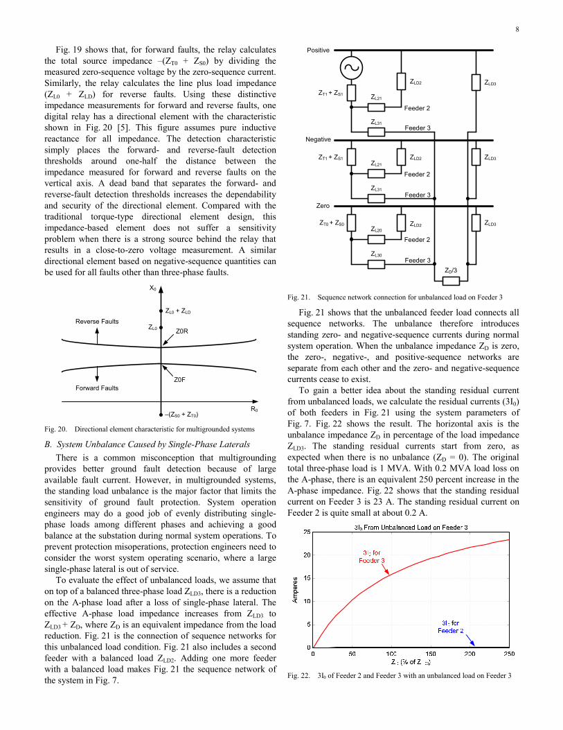
To evaluate the effect of unbalanced loads, we assume that on top of a balanced three-phase load ZLD3, there is a reduction on the A-phase load after a loss of single-phase lateral. The effective A-phase load impedance increases from ZLD3 to ZLD3 + ZD, where ZD is an equivalent impedance from the load reduction. Fig. 21 is the connection of sequence networks for this unbalanced load condition. Fig. 21 also includes a second feeder with a balanced load ZLD2. Adding one more feeder with a balanced load makes Fig. 21 the sequence network of the system in Fig. 7.

ZT1 + ZS1

ZLD3

ZL21

ZLD2

ZT1 + ZS1 ZLD3ZLD2

ZT0 + ZS0 ZLD2

ZL31

ZLD3

ZL21

ZL31

ZL20

ZL30

ZD/3

Positive

Negative

Zero

Feeder 2

Feeder 3

Feeder 2

Feeder 3

Feeder 2

Feeder 3

Fig. 21. Sequence network connection for unbalanced load on Feeder 3

Fig. 21 shows that the unbalanced feeder load connects all sequence networks. The unbalance therefore introduces standing zero- and negative-sequence currents during normal system operation. When the unbalance impedance ZD is zero, the zero-, negative-, and positive-sequence networks are separate from each other and the zero- and negative-sequence currents cease to exist.

To gain a better idea about the standing residual current from unbalanced loads, we calculate the residual currents (3I0) of both feeders in Fig. 21 using the system parameters of Fig. 7. Fig. 22 shows the result. The horizontal axis is the unbalance impedance ZD in percentage of the load impedance ZLD3. The standing residual currents start from zero, as expected when there is no unbalance (ZD = 0). The original total three-phase load is 1 MVA. With 0.2 MVA load loss on the A-phase, there is an equivalent 250 percent increase in the A-phase impedance. Fig. 22 shows that the standing residual current on Feeder 3 is 23 A. The standing residual current on Feeder 2 is quite small at about 0.2 A.

Fig. 22. 3I0 of Feeder 2 and Feeder 3 with an unbalanced load on Feeder 3

9

C. Fault Resistance Coverage In multigrounded systems, the ground fault detection

sensitivity is not limited by digital relay sensitivity and instrument transformer accuracy. Rather, the worst possible feeder unbalance limits the ground fault resistance coverage.

Using the results from Section V, Subsection B, a 23 A residual current from unbalanced loads is equivalent to a fault current generated by a ground fault with a 320 Ω fault resistance for a 12.5 kV system. That is, on such a system, the ground fault resistance coverage cannot be larger than 320 Ω.

There are other factors limiting the ground fault detection sensitivity. These factors include coordinating a substation protection device with downstream reclosers and fuses and avoiding cold load pickup and transformer energization inrush currents. These considerations further increase the ground fault overcurrent element pickups and reduce the fault resistance coverage. A ground fault relay pickup setting is normally between 100 and 300 A [13], which translates to a maximum 72 Ω fault resistance coverage on a 12.5 kV system.

Reference [14] discusses high-impedance faults and their detection. High-impedance faults are a special concern on multigrounded systems because the fault currents are typically under 100 A and below the ground fault protection current pickup level. A main cause of high-impedance faults is downed power conductors. The fault currents of downed-conductor high-impedance faults depend upon the ground surface materials. The fault current can be anywhere from 0 A from an asphalt surface to less than 80 A from a reinforced concrete surface. A downed-conductor high-impedance fault poses a public hazard if it is not isolated in a timely manner.

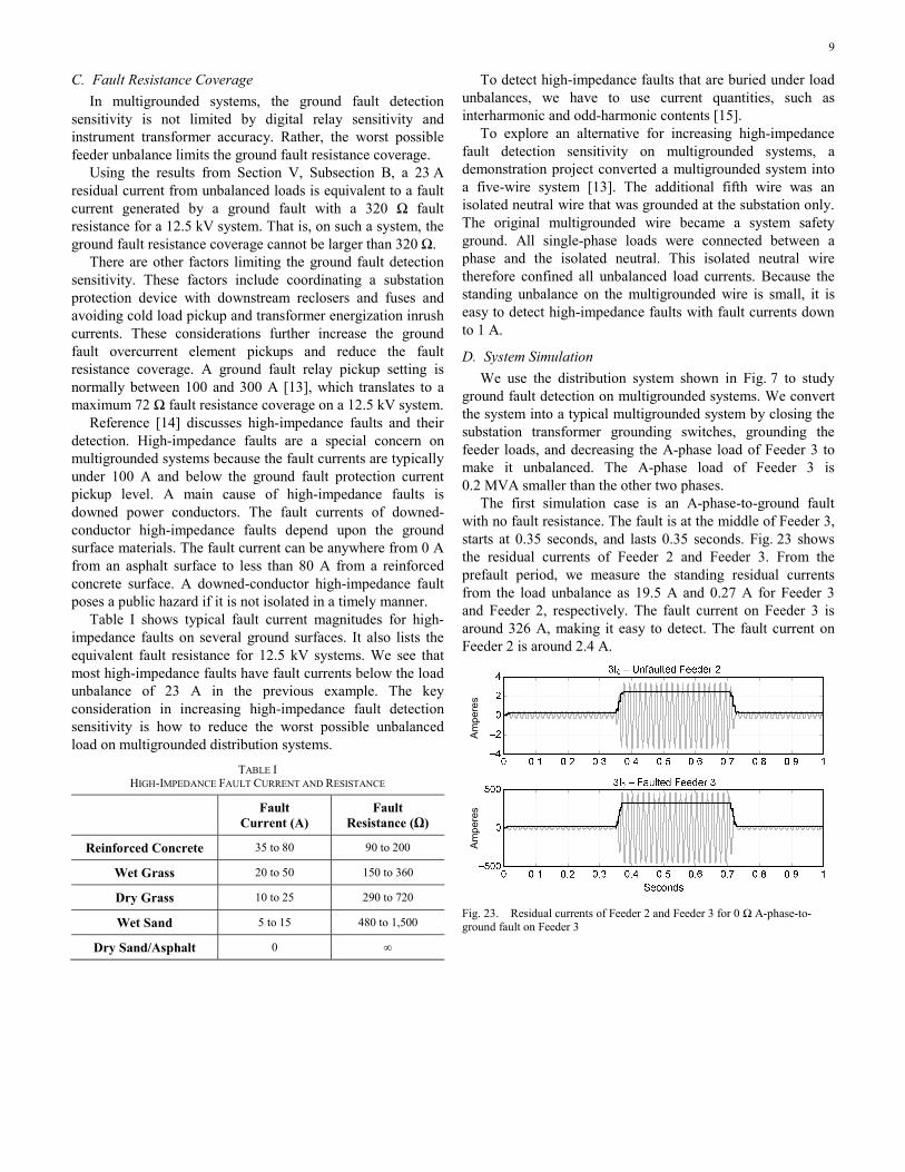
Table I shows typical fault current magnitudes for high-impedance faults on several ground surfaces. It also lists the equivalent fault resistance for 12.5 kV systems. We see that most high-impedance faults have fault currents below the load unbalance of 23 A in the previous example. The key consideration in increasing high-impedance fault detection sensitivity is how to reduce the worst possible unbalanced load on multigrounded distribution systems.

TABLE I HIGH-IMPEDANCE FAULT CURRENT AND RESISTANCE

Fault Current (A)

Fault Resistance (Ω)

Reinforced Concrete 35 to 80 90 to 200

Wet Grass 20 to 50 150 to 360

Dry Grass 10 to 25 290 to 720

Wet Sand 5 to 15 480 to 1,500

Dry Sand/Asphalt 0 ∞

To detect high-impedance faults that are buried under load unbalances, we have to use current quantities, such as interharmonic and odd-harmonic contents [15].

To explore an alternative for increasing high-impedance fault detection sensitivity on multigrounded systems, a demonstration project converted a multigrounded system into a five-wire system [13]. The additional fifth wire was an isolated neutral wire that was grounded at the substation only. The original multigrounded wire became a system safety ground. All single-phase loads were connected between a phase and the isolated neutral. This isolated neutral wire therefore confined all unbalanced load currents. Because the standing unbalance on the multigrounded wire is small, it is easy to detect high-impedance faults with fault currents down to 1 A.

D. System Simulation We use the distribution system shown in Fig. 7 to study

ground fault detection on multigrounded systems. We convert the system into a typical multigrounded system by closing the substation transformer grounding switches, grounding the feeder loads, and decreasing the A-phase load of Feeder 3 to make it unbalanced. The A-phase load of Feeder 3 is 0.2 MVA smaller than the other two phases.

The first simulation case is an A-phase-to-ground fault with no fault resistance. The fault is at the middle of Feeder 3, starts at 0.35 seconds, and lasts 0.35 seconds. Fig. 23 shows the residual currents of Feeder 2 and Feeder 3. From the prefault period, we measure the standing residual currents from the load unbalance as 19.5 A and 0.27 A for Feeder 3 and Feeder 2, respectively. The fault current on Feeder 3 is around 326 A, making it easy to detect. The fault current on Feeder 2 is around 2.4 A.

Am

pere

sA

mpe

res

Fig. 23. Residual currents of Feeder 2 and Feeder 3 for 0 Ω A-phase-to-ground fault on Feeder 3

10

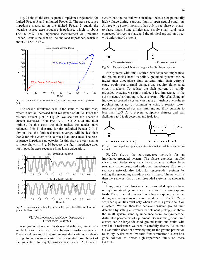
Fig. 24 shows the zero-sequence impedance trajectories for faulted Feeder 3 and unfaulted Feeder 2. The zero-sequence impedance measured on the faulted Feeder 3 equals the negative source zero-sequence impedance, which is about 1.56∠83.2° Ω. The impedance measurement on unfaulted Feeder 2 equals the sum of line and load impedance, which is about 224.5∠42.1° Ω.

Zero-Sequence Impedance180

160

140

120

100

80

60

40

20

0

R (Ω)160140120100806040200

Z0 for Feeder 2 (Reverse Fault)

Z0 for Feeder 3 (Forward Fault)

Fig. 24. Z0 trajectories for Feeder 3 (forward fault) and Feeder 2 (reverse fault)

The second simulation case is the same as the first case, except it has an increased fault resistance of 200 Ω. From the residual current plot in Fig. 25, we see that the Feeder 3 current decreases from 19.5 A to 18.2 A after the fault initiates. In this case, the fault makes the feeder more balanced. This is also true for the unfaulted Feeder 2. It is obvious that the fault resistance coverage will be less than 200 Ω for this system with so much load unbalance. The zero-sequence impedance trajectories for this fault are very similar to those shown in Fig. 24 because the fault impedance does not impact the zero-sequence impedance calculation.

3I0 – Unfaulted Feeder 2

3I0 – Faulted Feeder 3

Am

pere

sA

mpe

res

Seconds

–0.4

–0.2

0

0.2

0.4

40

20

0

–20

–400 0.1 0.2 0.3 0.4 0.5 0.6 0.7 0.8 0.9 1

0 0.1 0.2 0.3 0.4 0.5 0.6 0.7 0.8 0.9 1

Fig. 25. Residual currents of Feeder 2 and Feeder 3 for 200 Ω A-phase-to-ground fault on Feeder 3

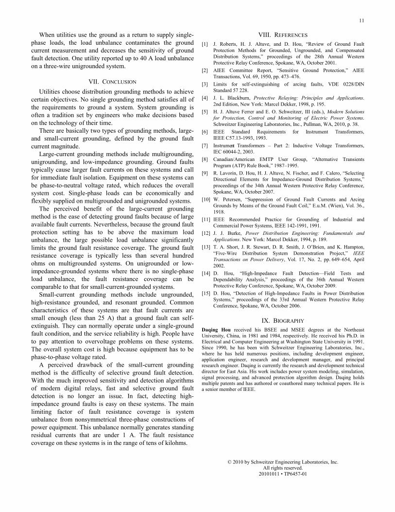
VI. UNIGROUNDED AND LOW-IMPEDANCE- GROUNDED SYSTEMS

A unigrounded system has its neutral solidly grounded at a single location, usually at the substation transformer neutral. There are three- and four-wire unigrounded systems, as shown in Fig. 26. A four-wire system has its neutral brought out of the substation to supply single-phase loads. A four-wire

system has the neutral wire insulated because of potentially high voltage during a ground fault or open-neutral condition. A three-wire system normally has only three-phase or phase-to-phase loads. Some utilities also supply small rural loads connected between a phase and the physical ground on three-wire unigrounded systems.

a. Three-Wire System b. Four-Wire System

Fig. 26. Three-wire and four-wire unigrounded distribution systems

For systems with small source zero-sequence impedance, the ground fault current on solidly grounded systems can be higher than three-phase fault currents. High fault currents cause equipment thermal damage and require higher-rated circuit breakers. To reduce the fault current on solidly grounded systems, we can introduce a low impedance in the system neutral grounding path, as shown in Fig. 27a. Using an inductor to ground a system can cause a transient overvoltage problem and is not as common as using a resistor. Low-impedance-grounded systems limit ground fault currents to less than 1,000 A to prevent equipment damage and still facilitate rapid fault detection and isolation.

Fig. 27. Low-impedance-grounded distribution system and its zero-sequence network

Fig. 27b shows the zero-sequence network for an impedance-grounded system. The figure excludes parallel system and feeder stray capacitance because of their large reactance values compared with other impedances. This zero-sequence network also holds for unigrounded systems by setting the grounding impedance (Z) to zero. The network is then the same as that of multigrounded systems, as shown in Fig. 18.

Unigrounded and low-impedance-grounded systems have no system standing unbalance generated by single-phase loads. There is no interconnection between sequence networks during normal system operation, as shown in Fig. 21. Zero-sequence quantities exist only when there is a ground fault on a system. We can therefore achieve sensitive ground fault detection by setting an overcurrent element pickup just above the small system standing unbalance from nonsymmetrical distributed parameters of equipment. Because the ground fault current can be large for solid ground faults and faults with small fault resistance, we need to carefully size the CT so that CT saturation does not adversely impact the ground protection reliability. A dedicated low-ratio flux-summation CT can be a good solution to detect high-impedance faults on these systems.

11

When utilities use the ground as a return to supply single-phase loads, the load unbalance contaminates the ground current measurement and decreases the sensitivity of ground fault detection. One utility reported up to 40 A load unbalance on a three-wire unigrounded system.

VII. CONCLUSION Utilities choose distribution grounding methods to achieve

certain objectives. No single grounding method satisfies all of the requirements to ground a system. System grounding is often a tradition set by engineers who make decisions based on the technology of their time.

There are basically two types of grounding methods, large-and small-current grounding, defined by the ground fault current magnitude.

Large-current grounding methods include multigrounding, unigrounding, and low-impedance grounding. Ground faults typically cause larger fault currents on these systems and call for immediate fault isolation. Equipment on these systems can be phase-to-neutral voltage rated, which reduces the overall system cost. Single-phase loads can be economically and flexibly supplied on multigrounded and unigrounded systems.

The perceived benefit of the large-current grounding method is the ease of detecting ground faults because of large available fault currents. Nevertheless, because the ground fault protection setting has to be above the maximum load unbalance, the large possible load unbalance significantly limits the ground fault resistance coverage. The ground fault resistance coverage is typically less than several hundred ohms on multigrounded systems. On unigrounded or low-impedance-grounded systems where there is no single-phase load unbalance, the fault resistance coverage can be comparable to that for small-current-grounded systems.

Small-current grounding methods include ungrounded, high-resistance grounded, and resonant grounded. Common characteristics of these systems are that fault currents are small enough (less than 25 A) that a ground fault can self-extinguish. They can normally operate under a single-ground fault condition, and the service reliability is high. People have to pay attention to overvoltage problems on these systems. The overall system cost is high because equipment has to be phase-to-phase voltage rated.

A perceived drawback of the small-current grounding method is the difficulty of selective ground fault detection. With the much improved sensitivity and detection algorithms of modern digital relays, fast and selective ground fault detection is no longer an issue. In fact, detecting high-impedance ground faults is easy on these systems. The main limiting factor of fault resistance coverage is system unbalance from nonsymmetrical three-phase constructions of power equipment. This unbalance normally generates standing residual currents that are under 1 A. The fault resistance coverage on these systems is in the range of tens of kilohms.

VIII. REFERENCES [1] J. Roberts, H. J. Altuve, and D. Hou, “Review of Ground Fault

Protection Methods for Grounded, Ungrounded, and Compensated Distribution Systems,” proceedings of the 28th Annual Western Protective Relay Conference, Spokane, WA, October 2001.

[2] AIEE Committee Report, “Sensitive Ground Protection,” AIEE Transactions, Vol. 69, 1950, pp. 473–476.

[3] Limits for self-extinguishing of arcing faults, VDE 0228/DIN Standard 57 228.

[4] J. L. Blackburn, Protective Relaying: Principles and Applications. 2nd Edition, New York: Marcel Dekker, 1998, p. 195.

[5] H. J. Altuve Ferrer and E. O. Schweitzer, III (eds.), Modern Solutions for Protection, Control and Monitoring of Electric Power Systems. Schweitzer Engineering Laboratories, Inc., Pullman, WA, 2010, p. 38.

[6] IEEE Standard Requirements for Instrument Transformers, IEEE C57.13-1993, 1993.

[7] Instrument Transformers – Part 2: Inductive Voltage Transformers, IEC 60044-2, 2003.

[8] Canadian/American EMTP User Group, “Alternative Transients Program (ATP) Rule Book,” 1987–1995.

[9] R. Lavorin, D. Hou, H. J. Altuve, N. Fischer, and F. Calero, “Selecting Directional Elements for Impedance-Ground Distribution Systems,” proceedings of the 34th Annual Western Protective Relay Conference, Spokane, WA, October 2007.

[10] W. Petersen, “Suppression of Ground Fault Currents and Arcing Grounds by Means of the Ground Fault Coil,” E.u.M. (Wien), Vol. 36., 1918.

[11] IEEE Recommended Practice for Grounding of Industrial and Commercial Power Systems, IEEE 142-1991, 1991.

[12] J. J. Burke, Power Distribution Engineering: Fundamentals and Applications. New York: Marcel Dekker, 1994, p. 189.

[13] T. A. Short, J. R. Stewart, D. R. Smith, J. O’Brien, and K. Hampton, “Five-Wire Distribution System Demonstration Project,” IEEE Transactions on Power Delivery, Vol. 17, No. 2, pp. 649–654, April 2002.

[14] D. Hou, “High-Impedance Fault Detection—Field Tests and Dependability Analysis,” proceedings of the 36th Annual Western Protective Relay Conference, Spokane, WA, October 2009.

[15] D. Hou, “Detection of High-Impedance Faults in Power Distribution Systems,” proceedings of the 33rd Annual Western Protective Relay Conference, Spokane, WA, October 2006.

IX. BIOGRAPHY Daqing Hou received his BSEE and MSEE degrees at the Northeast University, China, in 1981 and 1984, respectively. He received his Ph.D. in Electrical and Computer Engineering at Washington State University in 1991. Since 1990, he has been with Schweitzer Engineering Laboratories, Inc., where he has held numerous positions, including development engineer, application engineer, research and development manager, and principal research engineer. Daqing is currently the research and development technical director for East Asia. His work includes power system modeling, simulation, signal processing, and advanced protection algorithm design. Daqing holds multiple patents and has authored or coauthored many technical papers. He is a senior member of IEEE.

© 2010 by Schweitzer Engineering Laboratories, Inc. All rights reserved.

20101011 • TP6457-01