Embed Size (px)
Citation preview
Comparing Downlink Capacity between Super Wi-Fi
and Wi-Fi in Multi-Floored Indoor Environments
Gyumin Hwang
Department of Electrical Engineering
Graduate school of UNIST

Abstract
Super Wi-Fi is a Wi-Fi-like service exploiting TV white spaces (WS) via the cognitive radio technol-
ogy which is expected to achieve larger coverage than today’s Wi-Fi thanks to its superior propagation
characteristics. Super Wi-Fi is currently being materialized as an international standard, IEEE 802.11af,
targetting indoor and outdoor applications. This thesis demonstrates the potential of Super Wi-Fi in in-
door environments by measuring its signal propagation characteristics and comparing them with those of
Wi-Fi in the same indoor structure. Specifically, this thesis measures the wall and floor attenuation fac-
tors and path-loss distribution in 770 MHz and 2.4 GHz, and estimates the downlink capacity of Super
Wi-Fi and Wi-Fi according to wide-accepted indoor path loss models. The experimental results reveal
that TVWS signals can penetrate up to two floors and provide favorable coverage up to one floor above
and below. In addition, TVWS can not only extend the coverage of Wi-Fi but also significantly mitigate
shaded regions of Wi-Fi while achieving almost homogeneous data rates in the Wi-Fi’s coverage. The
observed phenomena imply that Super Wi-Fi may be suitable for indoor applications with requirements
of low-to-moderate data rates, extended horizontal and vertical coverage, and fair rate distribution within
the service coverage.


Contents
I. Introduction ….…………………………………………………………………………………… 1
II. Related Work ….……………………………………………………………………………….. 5
III. Preliminaries ……………………………………………………………………………………. 6
3.1 USRP ……………………………………………………………………………………..... 6
3.2 GNU Radio ……………………………………………………………………………….... 7
3.3 Path Loss Prediction Model ……………………………………………………………….. 7
IV. Experimental Setup …………………………………………………………………………… 12
4.1 Frequency & Antenna ……………………………………………………………………. 12
4.2 Locations & HW/SW Setup ……………………………………………………………… 13
V. Spectrum Characteristics Comparison between TVWS and ISM …………………………….. 15
5.1 Wall Attenuation Factor Comparison ……………………………………………………. 15
5.2 Floor Attenuation Factor Comparison …………………………………………………. 18
5.3 Single-Floor Signal Propagation Measurement ………………………………………... 20
5.4 Downlink Capacity Comparison ……………………………………………………….. 24
VI. Conclusion ………………………………………………………………………………….. 32
List of Figures
Figure 1-1. Frequency resource using pattern
Figure 1-2. Example of airtime fairness problem
Figure 3-1. Block diagram of USRP N210
Figure 3-2. Example of controlling USRP transmission power
Figure 3-3. Blocks of wide band FM receiver
Figure 3-4. Example of GNU Radio Companion
Figure 4-1. TVWS in Korea
Figure 4-2. Floor plan of the EB2 of UNIST
Figure 5-1. Picture of the walls used for measuring WAF
Figure 5-2. Description of WAF measurement procedure
Figure 5-3. WAF measurement result
Figure 5-4. FAF measurement procedure
Figure 5-5. FAF comparison between Super Wi-Fi and Wi-Fi
Figure 5-6. SNR measurement result at 2.401 GHz
Figure 5-7. SNR measurement result at 770 MHz
Figure 5-8. Setup for the SNR-bandwidth measurement
Figure 5-9. Result of the measurement to verify variation of SNR
Figure 5-10. Downlink capacity result
Figure 5-11. Downlink capacity of Super Wi-Fi without channel-bonding (6 MHz) in a single-
floor
Figure 5-12. Downlink capacity of Super Wi-Fi without 2 channel-bonding (12 MHz) in a
single-floor
Figure 5-13. Downlink capacity of Super Wi-Fi without 3 channel-bonding (24 MHz) in a
single-floor
Figure 5-14. Downlink capacity of Wi-Fi (20 MHz) in a single-floor

List of Tables
Table 2-1. Power loss coefficients, N, for indoor environments
Table 2-2. Floor attenuation factors, 𝐿𝑓(dB)
Table 4-1. Specification of walls
Table 4-2. Daughter board setting values
Table 4-3. Average SNR at the EB2 building of UNIST
Table 4-4. Path loss exponent of 770 MHz and 2.401 GHz
Table 4-5. Result of downlink capacity
Nomenclature
CR Cognitive Radio
UHD USRP Hardware Driver
DTV Digital TV
FAF Floor Attenuation Factor
ISM Industrial, Scientific and Medical
TVWS TV White Space
Rx Receiver
SDR Software Defined Radio
SNR Signal-to-Noise-Ratio
Tx Transmitter
UHF Ultra High Frequency
USRP Universal Software Radio Peripheral
U-NII Unlicensed National Information Instructure
VHF Very High Frequency
WAF Wall Attenuation Factor

Chapter 1
Introduction
In the past few decades, there has been a tremendous amount of incease in the number of wireless
devices including laptops, smart phones, and tablets. Such growth in wireless usage leads to the ever-
increasing demand to more spectrum, which is expected to cause spectrum scarcity in the near future due
to the limited spectrum resources with fair characteristics. However, it has been revealed that spectrum
scarcity is rooted at inefficient spectrum utilization as shown in Figure 1.1 [1] which is regarding the
usage pattern of spectrum resources in Washington DC during one month. As seen, most spectrum usage
is concentrated at certain spectrum bands, leaving others severely under-utilized.
Figure 1.1: Frequcny resource using pattern [1].
Cognitive radio (CR) is a promising technology that may resolve the spectrum scarcity by enhancing
the spectrum utilization. To utilize the spectrum, a CR device monitors spectrum bands and determines
which bands are temporarily unused by their incumbent users. The identified idle bands are utilized by
unlicensed CR users only when they are free of incumbent users, for which the CR users keep monitoring
1

the bands and evict them immediately at the return of the incumbents. Such behavior of CR devices has
been made possible thanks to the reprogrammable software defined radio (SDR) based design.
There exist some CR related standards, where IEEE 802.22 and IEEE 802.11af are two represen-
tative standards with different service scenarios – IEEE 802.22 is a wireless regional area network
(WRAN) standard aiming at serving the wireless Internet with up to 100 km coverage, while IEEE
802.11af builds upon the 802.11ac WLAN standard aiming at serving the wireless Internet with up to 5
km coverage which is often called Super Wi-Fi.
Super Wi-Fi is a TV White Space (TVWS)-based Wi-Fi service, which is similar to Wi-Fi. Wi-
Fi freely uses the industrial, scientific and medical (ISM) bands (2.4 GHz) and unlicensed national
information instructure (U-NII) bands (5 GHz) without any approval whereas Super Wi-Fi has to identify
an temporarily-idle channel in TVWS by using the CR technology to utilize the spectrum. TVWS refers
to unused frequency band of very high frequency (VHF) and ultra high frequency (UHF) which are
allocated for TV broadcasting, and this band is 54-698MHz in US and Korea. The FCC approved
that unlicensed user who observes the regulation uses TVWS as non-licensed band. Especially, the
switchover from analog television to digital television was an opportunity to extend its white space
(WS) in TV frequency band because digital transmission can transmit the same amount data using fewer
channels than analog transmission.
Super Wi-Fi has the superior frequency characteristics such as penetrability and path loss because it
is utilizing VHF and UHF bands that lie in much lower spectrum than ISM and U-NII. That is, Super
Wi-Fi is expected to be able to cover the same area with less power than Wi-Fi. In addition, it makes
it easier to manage the network and mitigates existing problems of Wi-Fi such as shaded areas and the
airtime fairness problem [2]. In particular, stations in Wi-Fi service area have dramatically different
data rates depending on their locations since Wi-Fi signals lose significant energy as they travel through
obstacles and uneven terrain. For example, Figure 1.2 [3] shows an example when nodes 1, 2 and 3
communicate at 11 Mbps with each other and the data rate R between nodes 4 and 5 is varied from 11
Mbps to 1 Mbps, the throughput of link 2-3 and link 4-5 are decreased because the link 4-5 occupies
more time as the data rate R is decreased.
In this thesis, we demonstrate the benefit of deploying Super Wi-Fi indoors by identifying its superior
characteristics to Wi-Fi via experimental studies. Although there exist various work modeling the indoor
signal propagation either at VHF/UHF bands [4, 5, 6, 7, 8] or at ISM/UNII bands, there have been no
result that compares the propagation characteristics of the two bands in the same indoor environment.
The contribution of this thesis is three-fold. First, we performed an extensive measurement study
that compares the signal propagation characteristics of Super Wi-Fi and Wi-Fi in the same indoor envi-
ronment, including wall and floor attenuation factors and path-loss exponents. Second, we demonstrate
2
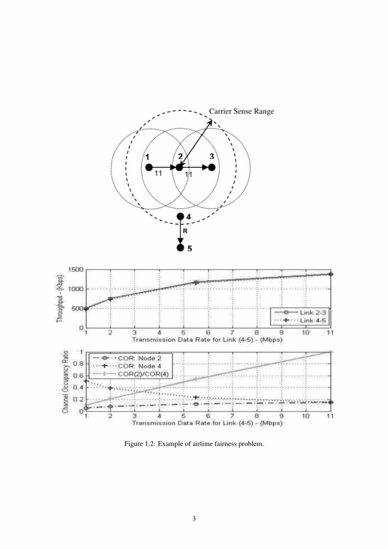
Figure 1.2: Example of airtime fairness problem.
3

the efficacy of exploiting TVWS for future indoor Wi-Fi applications such as extended coverage and
near-homogeneous achievable data rates. Lastly, we predict the coverage and average capacity of an
indoor Super Wi-Fi network by applying the experimental data to a path-loss model.
The rest of the thesis is organized as follows. Section 2 reviews related work, and Sections 3.1,
3.2 and 3.3 explain background knowledge about USRP, GNU Radio and path loss prediction models.
Sections 4.1 and 4.2 present the experimental setup. Sections 5.1 and 5.2 investigate the wall and floor
attenuation factors of TVWS and UNII bands, and Sections 5.3 and 5.4 describe the location-specific
signal-to-noise ratio (SNR) in the indoor environment and estimates average downlink capacity of Super
Wi-Fi and Wi-Fi. Finally, the thesis concludes with Section 6.
4

Chapter 2
Related Work
The indoor signal propagation has been characterized in many studies via field measurements in VHF,
UHF, and ISM bands. Zvanovec et al. [9] measured a received signal strength in 2.4 GHz and compared
it with a predicted received signal strength obtained from Multi-Wall propagation predict model. Ander-
son and Rappaport [10] measured a path loss and derived a path loss exponent from measurement in 2.5
and 60 GHz. Andrusenko et al. [11] conducted a path loss measurement in 30, 49 and 87.5 MHz. Seidel
and Rappaport [8] measured path loss in four types of buildings. Honcharenko et al. [5] also measured
path loss in office building. Gajewski et al. [12] conducted a floor attenuation factor measurement in
30, 49 and 87.5 MHz, and verified the General Urban Path Loss (GUPL) model published in [11] Taylor
et al. [13] measured a wall attenuation over 100 MHz to 3 GHz frequency range. Pena et al. [14] also
conducted a wall attenuation measurement in 900 MHz band. Nevertheless, none of them compared the
characteristics of TVWS and ISM bands in the same indoor environment.
Although Simic et al. [15] have compared indoor signal propagation of TVWS (630 MHz) and ISM
(2.4 GHz), their results are analytical predictions by a log-distance path loss model which are not based
on real measurements.
5
Chapter 3
Preliminaries
3.1 USRP
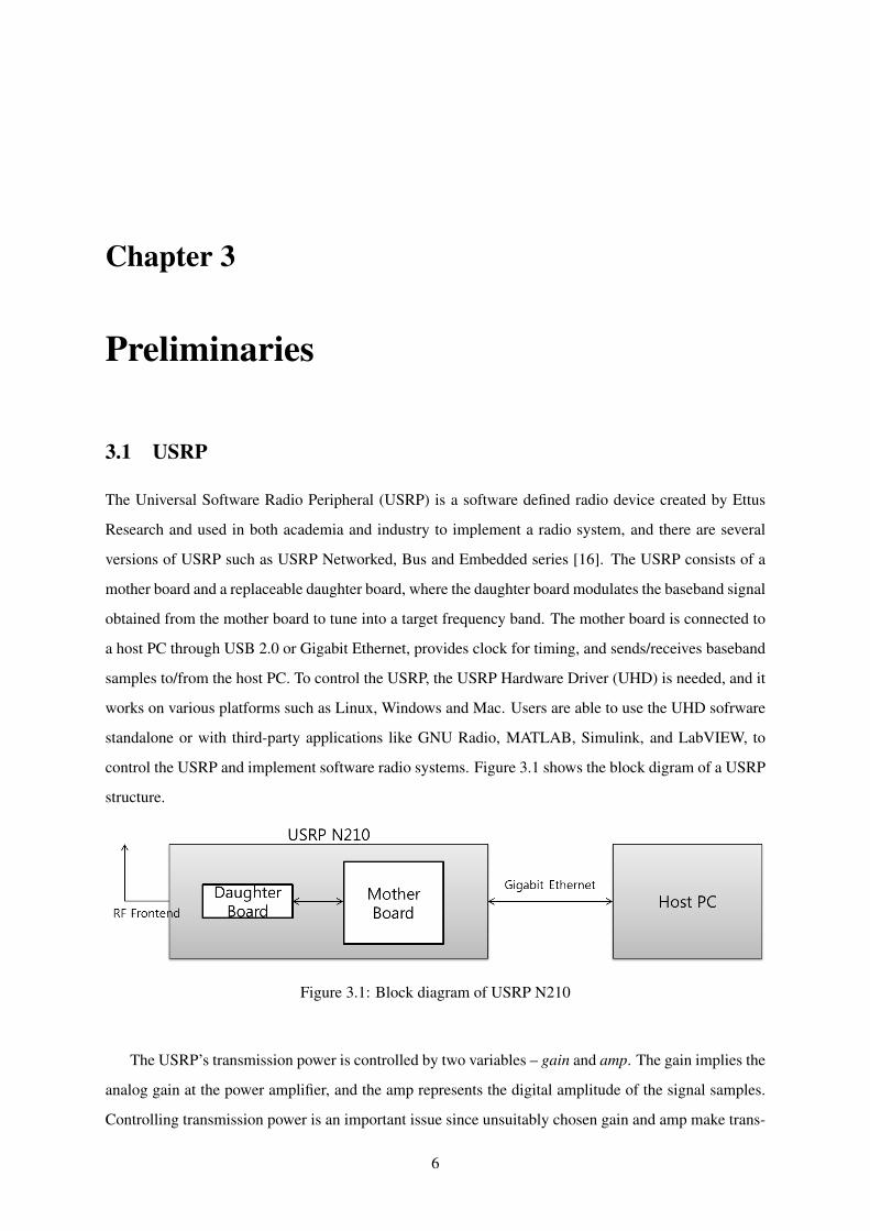
The Universal Software Radio Peripheral (USRP) is a software defined radio device created by Ettus
Research and used in both academia and industry to implement a radio system, and there are several
versions of USRP such as USRP Networked, Bus and Embedded series [16]. The USRP consists of a
mother board and a replaceable daughter board, where the daughter board modulates the baseband signal
obtained from the mother board to tune into a target frequency band. The mother board is connected to
a host PC through USB 2.0 or Gigabit Ethernet, provides clock for timing, and sends/receives baseband
samples to/from the host PC. To control the USRP, the USRP Hardware Driver (UHD) is needed, and it
works on various platforms such as Linux, Windows and Mac. Users are able to use the UHD sofrware
standalone or with third-party applications like GNU Radio, MATLAB, Simulink, and LabVIEW, to
control the USRP and implement software radio systems. Figure 3.1 shows the block digram of a USRP
structure.
Figure 3.1: Block diagram of USRP N210
The USRP’s transmission power is controlled by two variables – gain and amp. The gain implies the
analog gain at the power amplifier, and the amp represents the digital amplitude of the signal samples.
Controlling transmission power is an important issue since unsuitably chosen gain and amp make trans-
6

mission power dispersed out of the signal bandwidth thus resulting in incorrect SNR due to the increase
noise floor. Such a phenomenon is called out-of-band signal emission which is believed to be caused by
signal amplitude saturation at the analog power amplifier. Figure 3.2 illustrates the impact of gain and
amp. In the upper figure, the signal is a trapezoidal shape which can be easily detected and decoded at a
receiver. In the lower figure, however, the signal and noise have similar power thus making the receiver
hard to decode the signal. More details on the issue will be explained later in section 5.4.
USRP N210 is one of the USRP Networked series that provides 100 MS/s dual ADC and 400 MS/s
dual DAC. USRP N210 connects itself with a host PC through Gigabit Ethernet, which supports the
communication speed between the USRP and the host PC up to 50 MS/s. This kind of connection
method is much faster than older USRPs (e.g., USRP1) which connect themselves to a host PC through
USB 2.0 with up to 8 MS/s. USRP N210 also offers MIMO capability via a MIMO cable combining
two USRPs together.
3.2 GNU Radio
GNU Radio is a free and open-source development tool kit that provides signal processing blocks to
implement software radios [17]. Users can implement a software radio system by using GNU Radio
libraries and RF devices like USRP instead of expensive hardware radio systems, or by using GNU
Radio alone. The GNU Radio library consists of DSP blocks where they are wrriten in C++ to enhance
their performance. For flexible and convenient interface, SWIG wraps the blocks in Python, and users
can write a flow-graph (application) by creating and connecting blocks. Figure 3.3 shows the example
of a wide band FM receiver flow-graph.
GNU Radio also supports GUI-based development, called GNU Companion, with which user can
write a flow-graph by simply dragging and dropping blocks. Figure 3.4 shows a realization of the wide
band FM receiver in Figure 3.3.
3.3 Path Loss Prediction Model
In general, predicting path loss is a complicated task due to the random effect from the surrounding
environments such as multipath fading. To enhance the accuracy of prediction, there have been various
methods proposed. First, deterministic methods such as ray-tracing predict path loss according to the
physical law of wave propagation. Although the deterministic methods are usually quite accurate, they
need detailed information on the obstacles in the path of signal propagation and require a large amount
of time calculating the path loss. On the other hand, statistical methods such as Okumura-Hata [18],
7

Figure 3.2: Example of controlling USRP transmission power
8
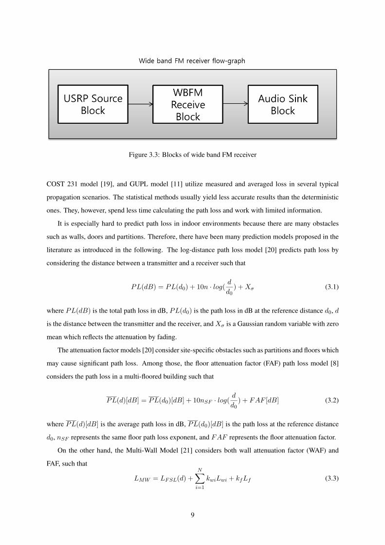
Figure 3.3: Blocks of wide band FM receiver
COST 231 model [19], and GUPL model [11] utilize measured and averaged loss in several typical
propagation scenarios. The statistical methods usually yield less accurate results than the deterministic
ones. They, however, spend less time calculating the path loss and work with limited information.
It is especially hard to predict path loss in indoor environments because there are many obstacles
such as walls, doors and partitions. Therefore, there have been many prediction models proposed in the
literature as introduced in the following. The log-distance path loss model [20] predicts path loss by
considering the distance between a transmitter and a receiver such that
PL(dB) = PL(d0) + 10n · log(d
d0) +Xσ (3.1)
where PL(dB) is the total path loss in dB, PL(d0) is the path loss in dB at the reference distance d0, d
is the distance between the transmitter and the receiver, and Xσ is a Gaussian random variable with zero
mean which reflects the attenuation by fading.
The attenuation factor models [20] consider site-specific obstacles such as partitions and floors which
may cause significant path loss. Among those, the floor attenuation factor (FAF) path loss model [8]
considers the path loss in a multi-floored building such that
PL(d)[dB] = PL(d0)[dB] + 10nSF · log(d
d0) + FAF [dB] (3.2)
where PL(d)[dB] is the average path loss in dB, PL(d0)[dB] is the path loss at the reference distance
d0, nSF represents the same floor path loss exponent, and FAF represents the floor attenuation factor.
On the other hand, the Multi-Wall Model [21] considers both wall attenuation factor (WAF) and
FAF, such that
LMW = LFSL(d) +N∑i=1
kwiLwi + kfLf (3.3)
9
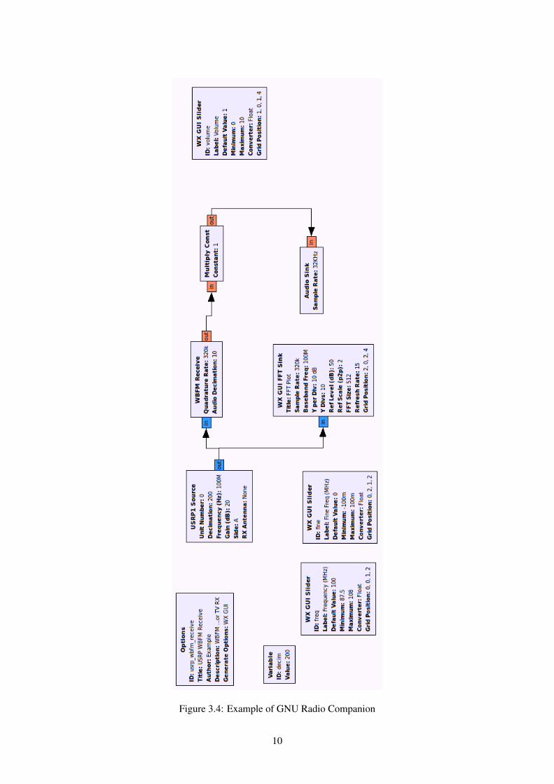
Figure 3.4: Example of GNU Radio Companion
10

where LMW is the path loss between a transmitter and a receiver in dB, LFSL is the free space path
loss at the distance of d meters in dB, N is the number of wall types, kwi is the number of i-th walls,
Lwi represents wall attenuation factor for i-th type wall, kf is the number of floors, and Lf is the floor
attenuation factor.
The ITU indoor path loss model [22] is intended to predict the path loss between a tranmitter and a
receiver in indoor environments and doesn‘t consider the wall attenuation factor. Its basic form is given
as
Ltotal = 20log10f +N · log10d+ Lf (n) − 28 (3.4)
where L is the total loss, N represents the distance power loss coefficient, f is frequency, d is the
distance in meters between the transmitter and the receiver, Lf is the floor attenuation loss in dB, and
n is the number of floors between the transmitter and the receiver. Typical parameters based on various
measurement results are given in Tables 3.1 and 3.2 [22].
These attenuation factor models draw a straight line between the transmitter and the receiver and
considers the number of floors and walls that the straight line encounters. This is called primary ray
tracing, and it has been shown that the primary ray tracing model predicts path loss quite accurately if
properly-chosen path loss exponents, FAF and WAF are used.
Frequency Residential Office Commercial900 MHz - 33 20
1.2 - 1.3 GHz - 32 221.8 - 2 GHz 28 30 22
4 GHz - 28 225.2 GHz - 31 -60 GHz - 22 17
Table 3.1: Power loss coefficients, N, for indoor environments
Frequency Residential Office Commercial
900 MHz -9 (1 floor)
19 (2 floors)24 (3 floors)
-
1.8 - 2 GHz 4n 15 + 4(n− 1) 6 + 3(n− 1)5.2 GHz - 16 (1 floor) -
Table 3.2: Floor attenuation factors, Lf (dB)
11

Chapter 4
Experimental Setup
The following sections describe the measurement setup for the wall attenuation factor (WAF), the floor
attenuation factor (FAF) and path loss measurements.
4.1 Frequency & Antenna
TVWS in Korea lies on 54-698 MHz (ch 2-51), and Figure 4.1 [23] shows TVWS in Korea and the
distribution of DTV channels. Subject to the Radio Regulation Law in Korea, we conduct our experi-
ments with 200 kHz bandwidth centered at 770 MHz frequency. Although this does not exactly match
a TVWS band, it is one of the closest frequency to TVWS allowed for experimental purpose in Ko-
rea. Other candidate frequencies includ 1134 and 1197 MHz with 650 kHz, and lower frequencies with
much narrower bandwidth. Although the chosen band has a limited bandwidth of 200 kHz which is
much narrower than the bandwidth of Super Wi-Fi and Wi-Fi (6-8 MHz and 20 MHz respectively), it
is free of wireless microphones that coexist in some parts of TVWS in Korea. As a result, there are no
interference in the 770 MHz in principle which has been also comfirmed by our measurements.
Wi-Fi lies over the industrial, scientific and medical (ISM) radio bands and the Unlicensed National
Information Infrastructure (U-NII) radio bands. To represent Wi-Fi, 2.401 GHz frequency band was
Figure 4.1: TVWS in Korea
12

Figure 4.2: Floor plan of the EB2 building of UNIST
selected which is within the ISM bands, because (i) the U-NII radio band suffers from more severe path
loss than ISM, and (ii) 2.401 GHz is in the gurad band of Wi-Fi channels so there exist no interfering
APs. Our measurements reveal that the level of interference from the Wi-Fi devices in the adjacent bands
is not substantial.
4.2 Locations and HW/SW Setup
All measurements were conducted on the third, fourth and fifth floors of the EB2 building of UNIST,
South Korea. The building was constructed in 2010 and consists of steel reinforced concrete with con-
structed marble floors, metal doors, and concrete and ply wood walls. The building has two staircases,
two elevators, and several utility rooms at the center of the building structure. Figure 4.2 shows the floor
plan.
In the near-field region, signal is radiated anomalistically because of the feedback to the transmitter.
Therefore, the minimum distance between a transmitter and a receiver should be larger than 2 meters to
avoid the near-field area effect, and the far-field area [24] γ is given as
γ > λ, if antenna is shorter than half of the wave length
γ > 2D2/λ, else(4.1)
where λ is the wavelength and D is the largest dimension of an antenna.
The length of the 770 MHz antenna we used is 14.6 cm while the wavelength λ of 770 MHz is 38.6
cm, thus resulting in the minimum distance of 78 cm. The length of the 2.401 GHz anttenna is 15 cm
and its wave length is 12.5 cm. As a result, the far-field area starts from 36 cm. However the far-field
area determined from measurements is about 1.7 meter which is larger than the theoretical ones, and
13

thus we have chosen 2 meters as the minimum distance between the transmitter and the receiver in our
experiments.
Throughout our measurements, we use the USRP N210 ith daughter boards of XCVR 2450, WBX,
and SBX. Four laptops are used as a host PC where each laptop is installed with Intel Core i7-2620M
(2.7 GHz, 2 cores), 8 GB RAM, 180 GB SSD, and Ubuntu 11.10. In addition, GNU Radio vesion 3.4.2
and UHD 003.003.000 are used, and the Raw OFDM [25] was used to transmit and receive OFDM
signals.
It is need to know the USRP transmission power and received signal strength to measure a WAF, FAF
and path loss, however, USRP can not measure a signal strength because it is an uncalibrated device.
Therefore we measured SNR instead of measuring signal strength, and connected two USRPs directly
through 50 Ω cable with a 50 dB attenuator to get the USRP transmission SNR. It is recommended to
use a attenuator at least 30 dB because connecting two USRPs without an attenuator would damage the
devices. As a result, the USRP transmission SNR was about 27.5 dB at 770 MHz and 2.401 GHz, which
means the original USRP transmission SNR was about 77.5 dB. This SNR was used for a reference SNR
of transmitters in the WAF, FAF and path loss measurements.
14

Chapter 5
Spectrum Characteristics Comparison
between TVWS and ISM
Super Wi-Fi has better penetrability than Wi-Fi thanks to its lower frequency which is particularly ben-
eficial when there are many obstacles such as walls, doors, and partitions as in indoor environments.
Therefore, it is expected that Super Wi-Fi would have wider coverage than Wi-Fi not only in outdoor
environments but also in indoor environments. The degree of penetration can be measured in many ways,
and WAF and FAF are two most typical metrics used in the literature. Although there have been many
measurement studies regarding WAF and FAF, none of them have measured them for TVWS bands and
ISM bands in the same indoor environment. In this chapter, we provide our measurement results on the
two metrics for the two representative frequencies, 770 MHz and 2.401 GHz.
5.1 Wall Attenuation Factor Comparison
There are four types of walls (including doors) in the fourth floor of the EB2 building at UNIST – metal
doors, thick and thin ply wood walls, and compound walls. Figure 4.2 presents the locations of the tested
walls where (a) is a metal door, (b) is a thick and thinply wood wall, (c) is a compound wall. Figure
5.1 shows the pictures of the listed walls. Table 5.1 shows the specification of the walls. The compound
wall consists of 97% ply wood and 3% metal.
Thickness (cm)Metal Door 5Thick Wall 123Thin Wall 18
Compound Wall 7.5
Table 5.1: Specification of walls
15

Figure 5.1: Picture of the walls used for measuring WAF
WAF can be determined by observing the difference in signal power measured in two cases – with
and without a wall between a transmitter and a receiver. In this thesis, SNR was used as a tool for the
WAF measurement assuming noise power is steady. WAF is obtained by using the Multi-Wall model
[20]:
PL(d)[dB] = PL(d0) + 10nMF · log(d
d0) +
∑WAF [dB] (5.1)
where PL(d) is the average path loss in dB at the distance d between the transmitter and the receiver,
PL(d0) represents the path loss at the reference distance d0, nMF denotes the measured path loss
exponent through multiple floors, and WAF is the attenuation factor by each wall. As mentioned in
the previous chapter, the USRP’s transmission SNR is 77.5 dB. Therefore, it is easy to know the path
loss PL(d) and PL(d0) at the distance d0 and d by measuring SNR at that distances, and we can obtain
WAF by setting the reference distance d0 as 2 meters because the distance d between the transmitter and
receiver was 2 meters. As a result, WAF is obtained by difference between the path losses at the distance
d and d0, since the log term is zero.
The transmitter and receiver were in opposite of each other. The tested wall is placed in the middle
of the transmitter and the receiver, and SNR is measured by moving the transmitter-receiver pair along
the wall in the step of 10 cm. The set of measurements is averaged out because the wall materials may
not be homogeneous. Figure 5.2 depicts the procedure of the WAF measurement.
The latitude of the transmitter and receiver antenna is set to 1.3 meter from the floor in all tests
except the test for the metal door. For the metal door, the measurements have benn conducted at 0.9
meter and 1.3 meter height to examine the impact of the small window on signal penetration. WBX and
XCVR2450 daughter boards are used for 770 MHz and 2.401 GHz measurements, respectively, and the
16

Figure 5.2: Discription of WAF measurement procedure
different gain and digital amp are set as in Table 5.2 because appropriate gain and amp depend on the
daughter board as mentiond previous section 3.1.
Table 5.2: Daughter board setting
WBX XCVR 2450Transmitter Gain (dB) 31 27
Receiver Gain (dB) 35 0Digital Amplitude 0.1 0.1
Figure 5.3 shows the result of WAF measurements for the four types of walls in 770 MHz and 2.401
GHz. As shown in the graph, 770 MHz has lower WAF than Wi-Fi for the all walls, and 770 MHz
penetrates the wall with very little loss. On the other hand, 2.401 GHz lose almost its power except for
the wood walls and lose more power than 770 MHz about 6 times for the metal door and about 10 times
for the compound wall.
17

Figure 5.3: WAF measurement result
5.2 Floor Attenuation Factor Comparison
For FAF measurements, the transmitter is fixed at the fifth floor while the receiver is moving along
the corridor of the third, fourth, and fifth floor up to the distance of 17 meters at the step of 30 cm.
The procedure of the FAF measurement is dipicted in Figure 5.4, and the measurement locations were
selected to avoid the staircases because the signals may travel along the staircase and affect the received
signal strength. The transmitter and the receiver are not placed directly below to avoid the null of
omnidirectional whip antenna [11]. The floor attenuation factor is defined as the difference between the
average SNR of the fifth floor and the averge SNR of the third or fourth floor. Figure 5.5 shows the result
that Super Wi-Fi has a smaller floor attenuation factor than Wi-Fi and can penetrates up to two floors
whereas Wi-Fi can penetrate only up to a single floor. Super Wi-Fi penetrates one floor with very little
signal loss with FAF of 0.635 dB, and its FAF over two floors is 9.88 dB. The Wi-Fi’s attenuation factor
for one floor is 12.76 dB which is even worse than the FAF Super Wi-Fi over the two floors. The result
of the FAF measurement implies that Super Wi-Fi can provide reliable signal strength even when users
are located at different floors.
18

Figure 5.4: FAF measurement procedure
Figure 5.5: FAF comparison between Super Wi-Fi and Wi-Fi
19

5.3 Single-Floor Signal Propagation Measurement
The path loss measurement was conducted on the fourth floor of the EB2 building at UNIST. The trans-
mitter is placed between elevators and a staircase, and its location is shown in Figure 4.2 (e). The
receiver is moved on the fourth floor at the step of 1 meter, where the receiver locations include the
whole hallways and two laboratory rooms. Although not all laboratory rooms are tested due to the
limited authorization, the tested rooms well capture the propagation characteristics of Super Wi-Fi and
Wi-Fi thanks to the symmetry of the building structure.
At each receiver location, SNR is measured 5 times by slightly changing each position by 10 cm
in order to average out the impact of fading. To manage the same transmission power in 770 MHz and
2.401 GHz, SBX daughter board has been adopted as it can cover both 770 MHz and 2.401 GHz. The
version of GNU Radio, RawOFDM, UHD, Ubuntu and laptop was the same as in the prior measurement
settings, and the transmitter and receiver gain is set to 12 dB and 31 dB respectively, amp is set as 0.4,
and the height of the transmitter/receiver is 1.3 meter.
Figures 5.6 and 5.7 illustrate the SNR measurement results of Super Wi-Fi and Wi-Fi. As shown,
the SNR of Super Wi-Fi is better than the SNR of Wi-Fi in most measurement locations, which implies
that Super Wi-Fi has a superior penetrability, diffraction, and path loss exponent than Wi-Fi. Table 5.3
is the average of the SNR measurement results.
770 MHz (dB) 2.401 GHz (dB)Room 17.272 6.417
Corridor 25.066 12.574Room + Corridor 20.389 8.88
Table 5.3: Average SNR at EB2 building of the UNIST
Path loss exponent in the fourth floor of EB2 building of the UNIST was calculated by using the
FAF path loss model [8]. Table 5.4 presents the categorized path loss exponent according to room and
corridor. As expected, the path loss exponent in corridor is smaller (thus better) than the path loss
exponent in room, thanks to the absence of obstacles and the waveguide effect.
Path Loss Exponent 770 MHz 2.401 GHzRoom 3.3345 5.1325
Corridor 2.4852 4.0947Room + Corridor 2.684 4.2188
Table 5.4: Path loss exponent of 770 MHz and 2.401 GHz
To eliminate the effect of WAF on path loss exponent, we calculated path loss exponenets by using
20
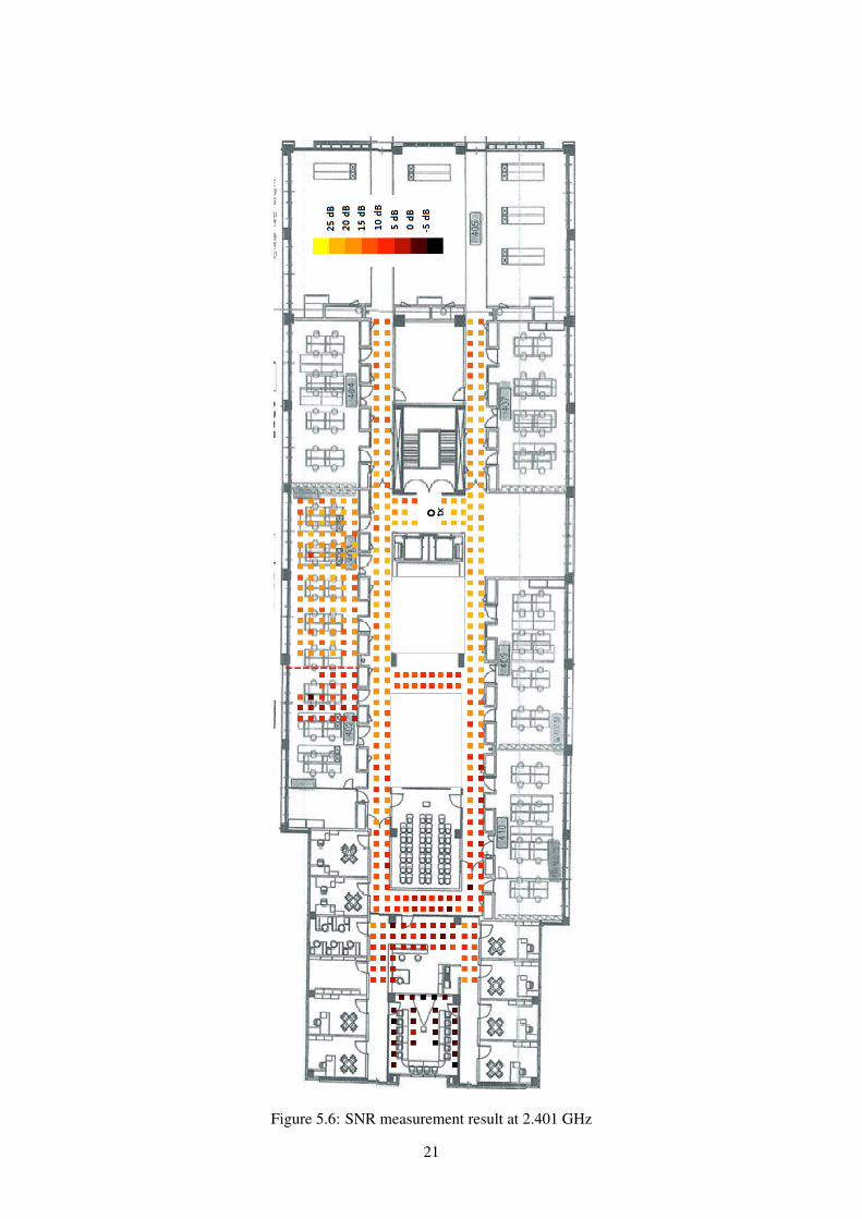
Figure 5.6: SNR measurement result at 2.401 GHz
21

Figure 5.7: SNR measurement result at 770 MHz
22

WAF path loss model in Eq. (5.1) at some locations. The locations are a portion of the area between the
two black lines in Figure 4.2. Such locations are affected by either metal door or thick ply wood wall.
In the considered scenario, we calculated two path loss exponents, by using (1) the model in Eq. (3.2)
excluding WAF where the effect of WAFs are integrated in the measured path loss exponent, and (2) the
model in Eq. (5.1) that specifies the WAFs of the metal door and the thick ply wood wall. The path loss
exponents from the first model are measured as 1.89 and 2.93 for 770 MHz and 2.401 GHz, respectively,
and the path loss exponents from the second model are predicted as 1.79 and 2.38 for 770 MHz and
2.401 GHz, respectively. Regarding 770 MHz, the difference between the two path loss exponents from
the models is only about 0.1 which is due to the small WAFs, i.e., 0.89 for the metal door and 1.95 for the
thick ply wood wall. In case of 2.401 GHz, however, the difference is around 1.65 and thus much larger
than in 770 MHz because of the large WAFs, i.e., 5.78 for the metal door and 11.01 for the thick ply
wood wall. In addition, the path loss exponent from the first model is always larger since the measured
exponent includes the additional path loss due to the walls.
23
5.4 Downlink Capacity
In estimating downlink capacity, we need to interprete the SNR measurements performed with 200 kHz
bandwidth in to the bandwidths of interest, i.e., 6, 12, and 24 MHz for Super Wi-Fi and 20 MHz for
Wi-Fi. To do so, it is critical to correctly understand how USRPs handle the gain parameter in setting its
transmission power. Although the USRP documentation states that the unit of the gain is dB, it does not
indicate what the reference metric is. Since Ettus Research does not provide detailed information in its
internal design, we have performed an experimental study to understand its internals reference value.
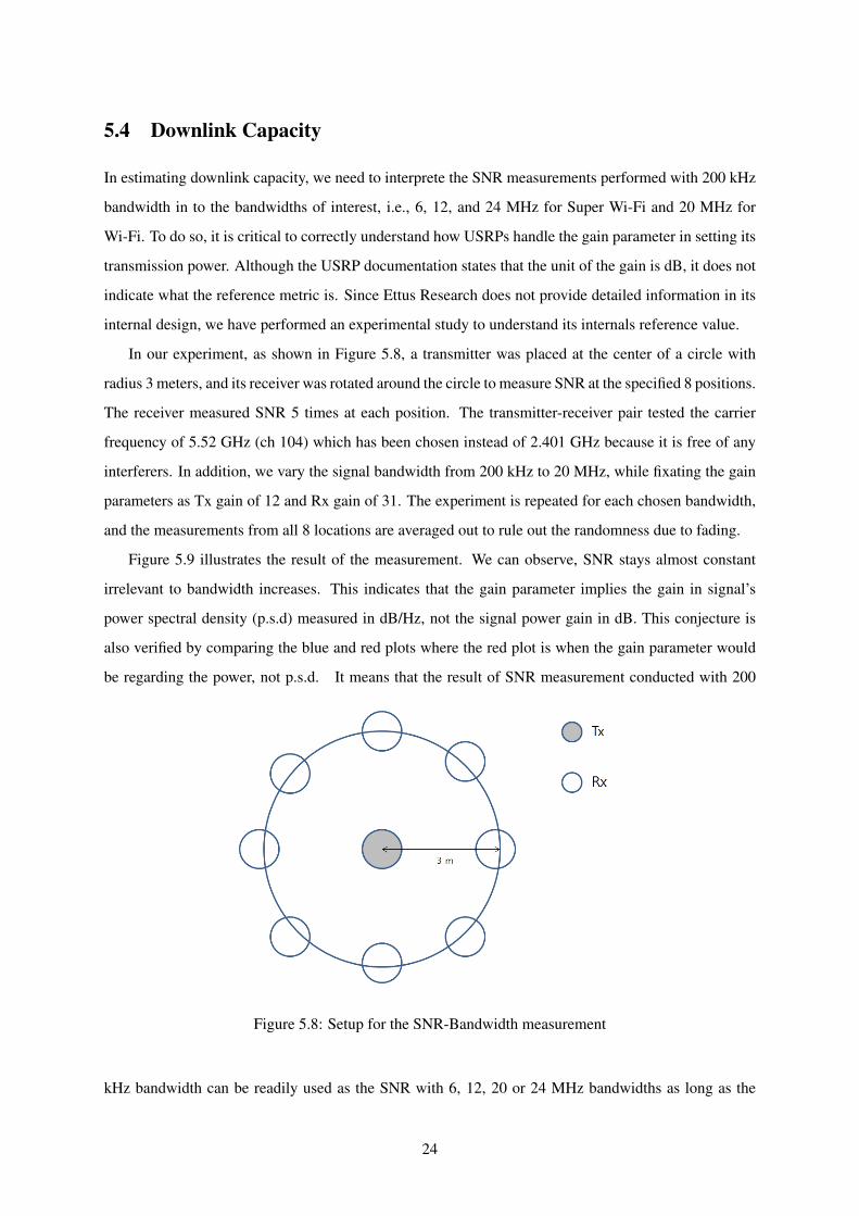
In our experiment, as shown in Figure 5.8, a transmitter was placed at the center of a circle with
radius 3 meters, and its receiver was rotated around the circle to measure SNR at the specified 8 positions.
The receiver measured SNR 5 times at each position. The transmitter-receiver pair tested the carrier
frequency of 5.52 GHz (ch 104) which has been chosen instead of 2.401 GHz because it is free of any
interferers. In addition, we vary the signal bandwidth from 200 kHz to 20 MHz, while fixating the gain
parameters as Tx gain of 12 and Rx gain of 31. The experiment is repeated for each chosen bandwidth,
and the measurements from all 8 locations are averaged out to rule out the randomness due to fading.
Figure 5.9 illustrates the result of the measurement. We can observe, SNR stays almost constant
irrelevant to bandwidth increases. This indicates that the gain parameter implies the gain in signal’s
power spectral density (p.s.d) measured in dB/Hz, not the signal power gain in dB. This conjecture is
also verified by comparing the blue and red plots where the red plot is when the gain parameter would
be regarding the power, not p.s.d. It means that the result of SNR measurement conducted with 200
Figure 5.8: Setup for the SNR-Bandwidth measurement
kHz bandwidth can be readily used as the SNR with 6, 12, 20 or 24 MHz bandwidths as long as the
24
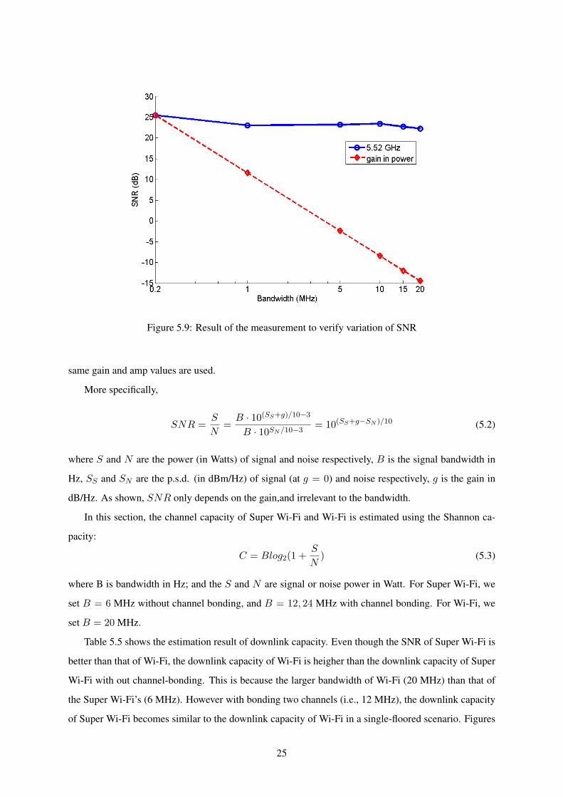
Figure 5.9: Result of the measurement to verify variation of SNR
same gain and amp values are used.
More specifically,
SNR =S
N=B · 10(SS+g)/10−3
B · 10SN/10−3= 10(SS+g−SN )/10 (5.2)
where S and N are the power (in Watts) of signal and noise respectively, B is the signal bandwidth in
Hz, SS and SN are the p.s.d. (in dBm/Hz) of signal (at g = 0) and noise respectively, g is the gain in
dB/Hz. As shown, SNR only depends on the gain,and irrelevant to the bandwidth.
In this section, the channel capacity of Super Wi-Fi and Wi-Fi is estimated using the Shannon ca-
pacity:
C = Blog2(1 +S
N) (5.3)
where B is bandwidth in Hz; and the S and N are signal or noise power in Watt. For Super Wi-Fi, we
set B = 6 MHz without channel bonding, and B = 12, 24 MHz with channel bonding. For Wi-Fi, we
set B = 20 MHz.
Table 5.5 shows the estimation result of downlink capacity. Even though the SNR of Super Wi-Fi is
better than that of Wi-Fi, the downlink capacity of Wi-Fi is heigher than the downlink capacity of Super
Wi-Fi with out channel-bonding. This is because the larger bandwidth of Wi-Fi (20 MHz) than that of
the Super Wi-Fi’s (6 MHz). However with bonding two channels (i.e., 12 MHz), the downlink capacity
of Super Wi-Fi becomes similar to the downlink capacity of Wi-Fi in a single-floored scenario. Figures
25

Figure 5.10: Downlink Capacity Result
5.11, 5.12, 5.13, and 5.14 present the impact of channel bonding via the following observations. First,
the downlink capacity of Wi-Fi is decreased dramatically when signal travels farther than 40 meters,
where the downlink capacity becomes worse than Super Wi-Fi without channel bonding. Second, Super
Wi-Fi supports stable downlink capacity all over its coverage. Third, the downlink capacity of Super
Wi-Fi with channel-bonding has much better downlink capacity than Wi-Fi. As a result, it is clear
that Super Wi-Fi can support stable downlink capacity all over its coverage and provide stations with
increased downlink capacity when Super Wi-Fi uses channel-bonding.
When signal penetrated over two floors, the downlink capaicty of Super Wi-Fi is always better than
the downlink capacity of Wi-Fi. Figure 5.10 compares there downlink capacities, and 5.5 shows the
specific result. We can not calculate the downlink capacity of Wi-Fi when signal penetrated two floors
because the 2.401 GHz signal was not received.
26

Figure 5.11: Donwlink capacity of Super Wi-Fi without channel-bonding (6 MHz) in a single-floor
27
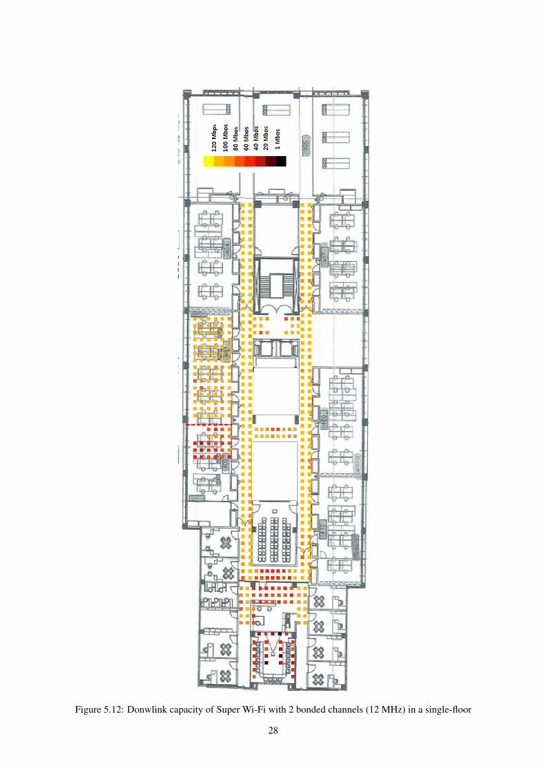
Figure 5.12: Donwlink capacity of Super Wi-Fi with 2 bonded channels (12 MHz) in a single-floor
28
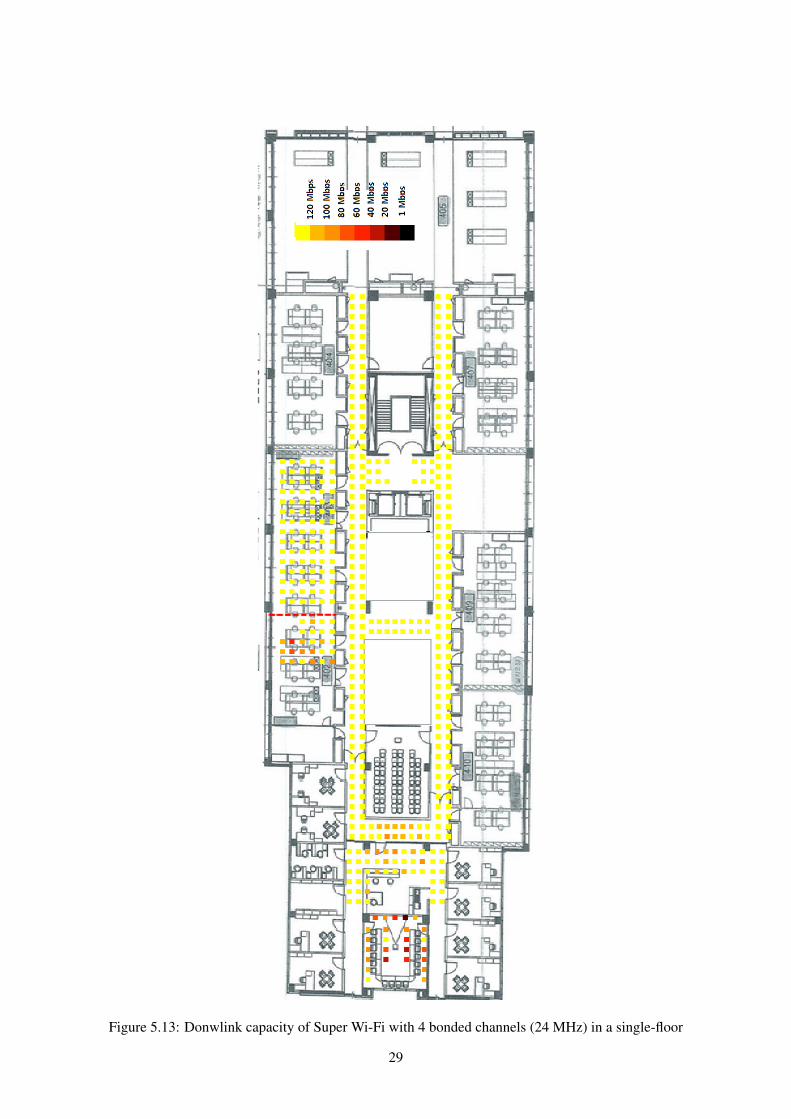
Figure 5.13: Donwlink capacity of Super Wi-Fi with 4 bonded channels (24 MHz) in a single-floor
29

Figure 5.14: Downlink capacity of Wi-Fi (20 MHz) in a single-floor
30

Same Floor Through 1 Floor Through 2 Floors
Super Wi-Fi (dB) (6 MHz)Room 34.75 33.61 18.47
Corridor 47.71 46.52 29.43Room + Corridor 39.93 38.77 22.86
Super Wi-Fi (dB) (12 MHz)Room 69.49 67.22 36.95
Corridor 95.43 92.03 58.86Room + Corridor 79.87 77.55 45.71
Super Wi-Fi (dB) (24 MHz)Room 138.99 134.45 73.89
Corridor 190.85 186.06 117.72Room + Corridor 159.73 155.09 91.43
Wi-Fi (dB) (20 MHz)Room 71.44 22.88
Corridor 96.66 34.34Room + Corridor 81.53 27.46
Table 5.5: Result of downlink capacity
31

Chapter 6
Conclusion
In this thesis, we have comapred the characteristics of Super Wi-Fi and Wi-Fi in the same indoor envi-
ronments in terms of WAF, FAF and path loss. Moreover, we have estimated the downlink capacity of
Super Wi-Fi and Wi-Fi indoors, based on the extensive path loss measurements. We have verified that
Super Wi-Fi has superior frequency characteristics than Wi-Fi such as better wall-penetration ability and
less path loss. As a result, it is expected that Super Wi-Fi provides wider coverage and more evenly-
distributed data rates within its coverage than today’s Wi-Fi. Without channel-bonding (6 MHz), Super
Wi-Fi achieves 48.97% of Wi-Fi’s downlink capacity (20 MHz) in a single-floored scenario and 141% at
one floor above or below where the transmitter is located. With two bonded channels (12 MHz), Super
Wi-Fi achieves 97% of Wi-Fi’s downlink capacity in a single-floored scenario and 282% at one floor
above or below scenario. Moreover, Super Wi-Fi with four bonded channels (24 MHz) achieves 195%
of Wi-Fi’s downlink capacity in a single floored environment and 564% at one floor above or below
environments. These results show that Super Wi-Fi has potential to become a successful application in
indoor environments.
It has been shown that Super Wi-Fi has the superior characteristics and can provide large enough
downlink capacity for indoor applications. By utilizing these advantages, new scenarios like coexisting
Wi-Fi with Super Wi-Fi can be considered as future direction of Super Wi-Fi research. Moreover, decid-
ing when is the best case to replace Wi-Fi with Super Wi-Fi in a single-floored environment is of great
interest, since it can improve not only the performance of Wi-Fi but also Super Wi-Fi’s performance.
In addition, it will be possible to predict whether it is useful to use Super Wi-Fi or not in given indoor
environment by developing a prediction mechanism.
32
REFERENCE
[1] Microsoft. Microsoft Spectrum Observatory. http://spectrum-observatory.cloudapp.net
[2] HYOIL KIM, K. S. A. C. J. 2013. Downlink Capacity of Super Wi-Fi Coexisting with
Conventional Wi-Fi. IEEE Global Communications Conference
[3] JOSHI, T., MUKHERJEE, A., YOO, Y. & AGRAWAL, D. P. 2008. Airtime fairness for IEEE
802.11 multirate networks. Mobile Computing, IEEE Transactions on, 7, 513-527
[4] ANDERSEN, J. B., RAPPAPORT, T. S. & YOSHIDA, S. 1995. Propagation measurements and
models for wireless communications channels. Communications Magazine, IEEE, 33, 42-49.
[5] HONCHARENKO, W., BERTONI, H. L., DAILING, J. L., QIAN, J. & YEE, H. 1992.
Mechanisms governing UHF propagation on single floors in modern office buildings. Vehicular
Technology, IEEE Transactions on, 41, 496-504.
[6] LAFORTUNE, J.-F & LECOURS, M. 1990 Measurement and modeling of propagation losses in a
building at 900 mhz. IEEE Trans. Veh. Technol. 39, 101–108.
[7] PORRAT, D. & COX, D. C. 2004. UHF propagation in indoor hallways. Wireless
Communications, IEEE Transactions on, 3, 1188-1198.
[8] SEIDEL, S. Y. & RAPPAPORT, T. S. 1992. 914 MHz path loss prediction models for indoor
wireless communications in multifloored buildings. Antennas and Propagation, IEEE Transactions
on, 40, 207-217.
[9] ZVANOVEC, S., PECHAC, P. & KLEPAL, M. 2003. Wireless LAN networks design: site survey
or propagation modeling? Radioengineering, 12, 42-49.
[10] ANDERSON, C. R. & RAPPAPORT, T. S. 2004. In-building wideband partition loss
measurements at 2.5 and 60 GHz. Wireless Communications, IEEE Transactions on, 3, 922-928.
[11] ANDRUSENKO, J., MILLER, R. L., ABRAHAMSON, J. A., MERHEB EMANUELLI, N. M.,
PATTAY, R. S. & SHUFORD, R. M. 2008. VHF general urban path loss model for short range
ground-to-ground communications. Antennas and Propagation, IEEE Transactions on, 56, 3302-
3310.
[12] GAIEWSKI, P., SUCHAKISKI, P. K. & MATYSZKIEL, R. 2011. Prediction of VHF Radio
Wave Attenuation in an Urban Environmentl.
[13] TAYLOR, C. D., GUTIERREZ, S. J., LANGDON, S. L., MURPHY, K. L. & WALTON III, W.
A. 1997. Measurement of RF Propagation into Concrete Structures over the Frequency Range
100 MHZ to 3 GHz. Wireless Personal Communications. Springer.
[14] PENA, D., FEICK, R., HRISTOV, H. D. & GROTE, W. 2003. Measurement and modeling of
propagation losses in brick and concrete walls for the 900-MHz band. Antennas and Propagation,
IEEE Transactions on, 51, 31-39.
[15] SIMIC, L., PETROVA, M. & MAHONEN, P. Wi-Fi, but not on steroids: Performance analysis
of a Wi-Fi-like network operating in TVWS under realistic conditions. Communications (ICC),
2012 IEEE International Conference on, 2012. IEEE, 1533-1538.
[16] Ettus Research, Universal Software Radio Peripheral, http://ettus.com/
[17] GNU Radio, http://gnuradio.org/redmine/projects/gnuradio/wiki
[18] HATA, M. 1980. Empirical formula for propagation loss in land mobile radio services. Vehicular
Technology, IEEE Transactions on, 29, 317-325.
[19] COST. 1991. Urban Transmission Loss Models for Mobile Radio in the 900- and 1,800 MHz
Bands: (revision 2), COST 231.
[20] RAPPAPORT, T. S. 1996. Wireless communications: principles and practice, Prentice Hall PTR
New Jersey.
[21] ACTION, C. 1999. Digital Mobile Radio Towards Future Generation Systems: Final Report,
Directorate General Telecommunications, Information Society, Information Market, and
Exploitation Research.
[22] RECOMMENDATIONS, I. 2001. Propagation data and prediction methods for the planning of
indoor radio communication systems and radio local area networks in the frequency range
900MHz to 100GHz. ITU Recommendations.
[23] SUNGWOONG CHOI, S. C et al. 2011. Technology standard trends for utilization in tv white
space. Electronics and Telecommunications Trends 26, 68–78.
[24] SUCHANSKI, M., KANIEWSKI, P., MATYSZKIEL, R. & GAJEWSKI, P. Prediction of VHF
and UHF wave attenuation in urban environment. Microwave Radar and Wireless
Communications (MIKON), 2012 19th International Conference on, 2012. IEEE, 60-65.
[25] Jakubczak, S. K. 2010. RawOFDM, http://people.csail.mit.edu/szym/rawofdm/README.html

Acknowledgement
I would like to thank Prof. Hyoil Kim, Changhee Joo, Hyun Jong Yang and all members of WMNL.


![GSM Sniffing - TERAEXEteraexe.com/pdf/GSM-Sniffing.pdf · USRP-2 [20MHz] USRP-1 [8MHz] OsmocomBB [200 kHz] Focus of this talk Downlink Uplink Frequency coverage . Remove uplink filter](https://img.pdfslide.us/doc/110x75/6056272fa5f0ef3428602ebb/gsm-sniffing-usrp-2-20mhz-usrp-1-8mhz-osmocombb-200-khz-focus-of-this-talk.jpg)