Comparing apples and oranges

8 The Journal of Thoracic and Cardiovascular Surgery • January 2002

Mitral valve repair versus replacement, internal thoracic arteryversus saphenous vein graft conduits for coronary bypass,effect of chronic preoperative atrial fibrillation on outcome,gastric versus colon esophageal substitutes, complete versusincomplete off-pump revascularization, surgery in high- versuslow-volume centers, balloon versus surgical aortic valvotomy.

These are but a sample of studies of comparative outcome whose basis was clinicalexperience rather than a formal clinical trial. Often, a cursory glance at patient char-acteristics in each group reveals important differences that lead medical and statisti-cal reviewers and readers alike to scoff, “They’re comparing ‘apples and oranges!’”

What does it take to convince the skeptic that the difference in outcome attrib-uted to difference in treatment (or patient condition) is real? The answer to thisquestion is not academic; it can affect the way we as physicians learn to treat ourpatients from studies of clinical experience.

When comparison is made in the context of a properly designed, appropriate,ethical, feasible, well-analyzed, generalizable randomized trial, most of us wouldaccept a cause-and-effect linkage between treatment and difference in outcome. Incontrast, when the comparison emanates from studies of clinical experience—ubiq-uitous in surgical experience and reporting—cause-and-effect attribution is consid-ered “speculative” at best.

For 3 decades, multivariable risk factor analysis has been the mainstay for identi-fying and quantifying treatment outcome differences adjusted for patient characteris-tics. However, Kirklin and Barratt-Boyes1 recommended that these differences betreated as associations with outcomes, not causes. There is no guarantee that risk fac-tor analysis is an effective strategy for discovery of cause-and-effect mechanisms.2,3

During the 1980s, federal support for complex clinical trials in heart disease wasabundant. Few of us noticed important advances being made in statistical methodsfor valid, nonrandomized comparisons. An example of the advances was the semi-nal 1983 Biometrika article by Paul Rosenbaum at the University of Wisconsin,Madison, and Donald Rubin at the University of Chicago, “The Central Role of thePropensity Score in Observational Studies for Causal Effects.”4 In the 1990s, as thefunding climate changed, interest in methods for making nonrandomized compar-isons accelerated.5-10

Recently, these methods have been recommended by statistical reviewers forcomparative clinical studies and have been adopted by some clinical researchgroups. The result has been the introduction into our literature of unfamiliar meth-ods with their unfamiliar terminology. Rather than being relieved that at last apples-to-apples comparisons can be made with rigor, medical and sometimes statisticalreviewers, as well as readers, have become bewildered!

From the Departments of Thoracic andCardiovascular Surgery and Biostatistics andEpidemiology, The Cleveland ClinicFoundation, Cleveland, Ohio.

Received for publication Dec 13, 2000;accepted for publication July 31, 2001.

Address for reprints: Eugene H. Blackstone,MD, The Cleveland Clinic Foundation, 9500Euclid Ave, Desk F25, Cleveland, OH 44195(E-mail: [email protected]).

J Thorac Cardiovasc Surg 2002;123:8-15

Copyright © 2002 by The AmericanAssociation for Thoracic Surgery

0022-5223/2002 $35.00 + 0 12/1/120329

doi:10.1067/mtc.2002.120329

Comparing apples and orangesEugene H. Blackstone, MD

Statisticsfor theRest of Us

Blackstone Statistics for the Rest of Us

The Journal of Thoracic and Cardiovascular Surgery • Volume 123, Number 1 9

TXET

CSP

ACD

CHD

GTS

EDIT

ORI

AL

Therefore, my purpose is to (1) clarify the nature of theproblem in nonrandomized comparisons that gives rise toapples-and-oranges skepticism; (2) review previousattempts to solve the problem; (3) present a method knownas balancing scores that can achieve apples-to-apples com-parisons under some nonrandomized conditions; (4)describe in nontechnical detail construction of the simplestbalancing score, the propensity score; (5) demonstrate howthe propensity score is used; and (6) discuss limitations, pit-falls, and alternatives.

Nature of the ProblemExcept by chance, characteristics differ among patientsconstituting comparison groups of interest in nonrandom-ized studies. (For lack of a better term, I use the phrase com-parison group of interest throughout the text to indicateeither a treatment or procedure difference of interest or apatient characteristic difference of interest, such as whethera patient is in chronic atrial fibrillation). These differencesin characteristics between groups are often large, system-atic, and statistically significant. They arise from clinicallymotivated patient selection. (How often does the clinicalinferences section of a journal article begin, “In carefullyselected patients. . . ?”) They arise for undocumented rea-sons called “treatment variance.” They sometimes arise bychance. In whatever way they arise, they invalidate directcomparisons.

For example, Table 1 contrasts a few characteristics ofpatients referred for stress echocardiography who reportedthey either were or were not receiving long-term aspirintherapy. A clinically relevant question might be, “Doeslong-term aspirin use convey a survival benefit, and if so,for whom?” However, a glance at the table of patient char-acteristics makes the reader justifiably suspicious ofattributing outcome difference to aspirin treatment in suchobviously selected patients. “True, true, and unrelated,”says one. “Apples and oranges,” says another.

Comparisons based on well-designed randomized studiesprovide at least 6 protections not available to the clinicalinvestigator that increase the cause-effect believability of acomparison.11,12 (1) Entry and exclusion criteria are pre-scribed and identical for the groups being compared; thus,the variables used to assign treatment are known. (2) Allpatients have a specified chance of receiving each treatment,avoiding both obvious and nonobvious clinical selection ofpatients for one treatment or the other. (3) Treatments areconcurrent, avoiding temporal trends. (4) Data collection isconcurrent, uniform, and high quality, eliminating differ-ences in definition or types of variables collected. (5)Unrecorded variables affecting outcome are nearly equallydistributed between groups, eliminating confounding (one ofthe most important benefits of randomization). (6)Assumptions underlying statistical comparison tests are met.

None of these protections is available in making nonran-domized comparisons. So, why not mount randomized trialsfor every question? Without elaborating the limitations of ran-domized trials (but pointing out that some comparisons, suchas whether or not a person goes into atrial fibrillation, cannotbe randomized), let us acknowledge that it is impossible tomount a randomized trial to address every comparison.13

Can anything be done to increase the credibility of com-parative studies based on clinical experience rather thanrandomized trials?

Previous Attempts to Address the ProblemMatchingA possibly familiar method for making nonrandomizedcomparisons is the case-control study.14,15 The methodseems logical and straightforward in concept. Patients inone treatment group (cases) are matched with one or morepatients in the other treatment group (controls) according tovariables such as age, sex, and ventricular function.However, case matching is rarely easy in practice. Howclose in age is acceptable? How close in ejection fraction?“We don’t have anyone to match this patient in both age andejection fraction!” The more variables that need to bematched, the more difficult it is to find a match in all spec-ified characteristics! Yet, matching on only a few variablesmay not protect well against apples-and-oranges compar-isons.16-18 Diabolically, selection factor effects (calledbias), which case-matching is intended to reduce, mayincrease bias if unmatched cases are simply eliminated.19

Multivariable AnalysisTreatment differences in outcome may instead be identifiedby multivariable analysis. Such analyses examine manyvariables simultaneously, including the comparison variableof interest. If one is fortunate, multivariable analysis willeliminate selection factors and provide an accurate assess-ment of the effect of the comparison variable of interest,

TABLE 1. Selected patient characteristics according tolong-term aspirin use in patients undergoing stressechocardiography for known or suspected coronary arterydisease

ASA No ASAPatient characteristic (n = 2455) (n = 4072) P

Men (%) 49 56 .001Age (y, mean ± SD) 62 ± 11 56 ± 12 <.0001Smoker (%) 10 13 .001Resting heart rate (beats/min) 74 ± 13 78 ± 14 <.0001Ejection fraction (%) 50 ± 9 53 ± 7 <.0001

ASA, Long-term aspirin use; SD, standard deviation.


Statistics for the Rest of Us Blackstone

EDITO

RIAL

CHD

GTS

ACD

ETCSP

TX

properly adjusted for patient characteristic differences.However, until now there has been no test to determinewhether we have been fortunate.2,18,20,21

Balancing Scores to the RescueApples-to-apples nonrandomized comparisons of outcomecan be achieved, within certain limitations, by use of so-called balancing scores.4 Balancing scores are a class ofmultivariable statistical methods that identify patients withsimilar chances of receiving one or the other treatment, per-mitting nonrandomized comparisons of treatment outcomes.

The developers of balancing score methods claim thatthe difference in outcome between patients who have a sim-ilar balancing score, but receive different treatments, pro-vides an unbiased estimate of the effect attributable to thecomparison variable of interest.4 That is technical jargon forsaying that the method can identify the apples from amongthe mixed fruit of clinical practice variance, transforming anapples-to-oranges outcomes comparison into an apples-to-apples comparison.22-25

Astonishing!

Why Is It Called a Balancing Score?Randomly assigning patients to alternative treatments inclinical trials balances both patient characteristics (at leastin the long run) and number of subjects in each treatmentarm. In a nonrandomized setting, neither patient character-istics nor number of patients is balanced for each treatment.A balancing score achieves local balance in patient charac-teristics at the expense of unbalancing n.

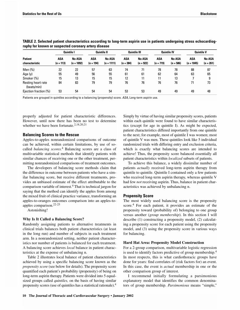
Table 2 illustrates local balance of patient characteristicsachieved by using a specific balancing score known as thepropensity score (see below for details). The propensity scorequantified each patient’s probability (propensity) of being onlong-term aspirin therapy. Patients were divided into 5 equal-sized groups called quintiles, on the basis of having similarpropensity scores (use of quintiles has a statistical rationale).4

Simply by virtue of having similar propensity scores, patientswithin each quintile were found to have similar characteris-tics (except for age in quintile I). As might be expected,patient characteristics differed importantly from one quintileto the next; for example, most of quintile I was women; mostof quintile V was men. These quintiles look like 5 individualrandomized trials with differing entry and exclusion criteria,which is exactly what balancing scores are intended toachieve! Thus, the propensity score balanced essentially allpatient characteristics within localized subsets of patients.

To achieve this balance, a widely dissimilar number ofpatients actually received long-term aspirin therapy fromquintile to quintile. Quintile I contained only a few patientswho received long-term aspirin therapy, whereas quintile Vhad few not receiving aspirin. Thus, balance in patient char-acteristics was achieved by unbalancing n.

Propensity ScoreThe most widely used balancing score is the propensityscore.4 For each patient, it provides an estimate of thepropensity toward (probability of) belonging to one groupversus another (group membership). In this section I willdescribe (1) constructing a propensity model, (2) calculat-ing a propensity score for each patient using the propensitymodel, and (3) using the propensity score in various waysfor balancing.

Hard Hat Area: Propensity Model ConstructionFor a 2-group comparison, multivariable logistic regressionis used to identify factors predictive of group membership.4

In most respects, this is what cardiothoracic groups havedone for years: find correlates of (risk factors for) an event.In this case, the event is actual membership in one or theother comparison group of interest.

I recommend initially formulating a parsimoniousexplanatory model that identifies the common denomina-tors of group membership. Parsimonious means “simple,”

TABLE 2. Selected patient characteristics according to long-term aspirin use in patients undergoing stress echocardiog-raphy for known or suspected coronary artery disease

Quintile I Quintile II Quintile III Quintile IV Quintile V

Patient ASA No ASA ASA No ASA ASA No ASA ASA No ASA ASA No ASAcharacteristic (n = 113) (n = 1092) (n = 194) (n = 1111) (n = 384) (n = 922) (n = 719) (n = 586) (n = 1045) (n = 261)

Men (%) 22 22 57 63 74 71 78 78 88 87Age (y) 55 49 56 55 61 61 62 64 63 65Smoker (%) 15 13 15 15 12 11 11 13 7 9Resting heart rate 84 83 79 79 76 76 76 76 71 73

(beats/min)Ejection fraction (%) 53 54 54 54 53 53 49 49 49 48

Patients are grouped in quintiles according to a balancing (propensity) score. ASA, Long-term aspirin use.



TXET

CSP

ACD

CHD

GTS

EDIT

ORI

AL

meaning a model limited to factors deemed statistically sig-nificant. Model means a mathematical representation orequation. (See the incremental risk factor concept in chap-ter 6 of Cardiac Surgery.1)

Once this traditional modeling is completed, a furtherstep is taken to generate the propensity model. The tradi-tional model is augmented by other factors, even if not sta-tistically significant. Thus, the propensity model is notparsimonious.22 The goal is to balance patient characteris-tics by incorporating “everything” recorded that may relateto either systematic bias or simply bad luck.17

When taken to the extreme, forming the propensity modelcan cause problems, because medical data tend to have manyvariables that measure the same thing. The solution is to pickone variable from among a closely related cluster of vari-ables as a representative of the cluster. For example, selectone variable representing body size from among height,weight, body surface area, and body mass index.

When a propensity model is being formed, informationshould not be thrown away. Some biostatistical collabora-tors dichotomize (group) continuous variables, such as ageor weight. This throws away information. Rather, thepropensity model should incorporate continuous variablesso as to produce a smooth distribution of scores necessaryfor good local matching.

Other construction tips are presented in the appendix.

Calculating the Propensity ScoreOnce the propensity modeling is completed, the propensityscore is calculated for each patient. The procedure is simi-lar to that used to calculate, for a given patient, expectedhospital mortality for coronary artery bypass grafting fromthe Society of Thoracic Surgeons risk equation.26

A logistic regression analysis, such as used for thepropensity model, generates a coefficient for each variable.The coefficient maps the units of measurement of the vari-able into units of risk.1 Specifically, a given patient’s valuefor a variable is transformed into risk units by multiplyingit by the coefficient. For example, if the coefficient is 1.13and the variable is “male” with a value of 1 (for “yes”), theresult will be 1.13 risk units. If the coefficient is 0.023 forthe variable “age” and a patient is 61.3 years old, 0.023times 61.3 is 1.41 risk units.

One continues through the list of model variables, multi-plying the coefficient by the specific value for each vari-able. When finished, the resulting products are summed. Tothis sum is added the intercept of the model. The final scoreis the propensity score. Its units are logit units, a wordcoined by Berkson,27 formerly of the Mayo Clinic.

Using the Propensity Score for ComparisonsOnce the propensity model is constructed and a propensityscore is calculated for each patient, 3 common types of

comparison are employed: matching, stratification, andmultivariable adjustment.

MatchingThe propensity score can be used as the sole criterion formatching pairs of patients.6,28

Rarely does one find exact matches. Instead, a patient isselected from the control group whose propensity score isnearest to that of a patient in the case group. If multiplepatients are close in propensity scores, optimal selectionamong these candidates can be used.23 Remarkably, problemsof matching on multiple variables disappear by compressing“everything known about the patient” into a single score!

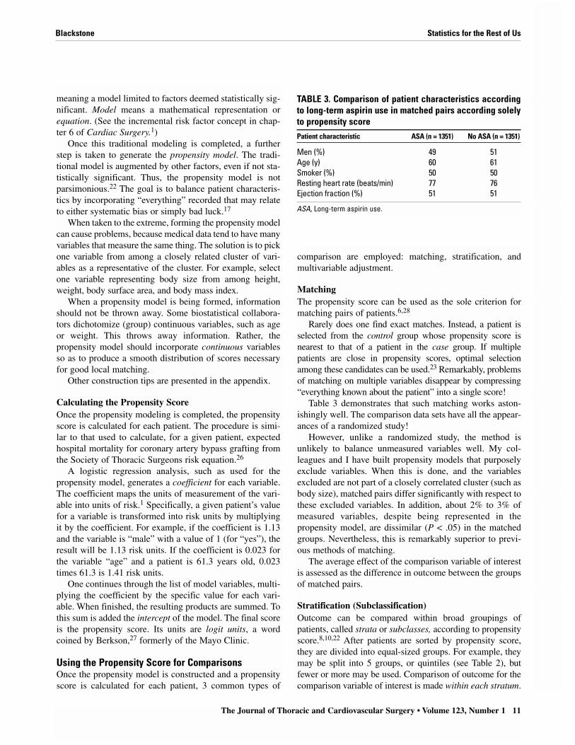
Table 3 demonstrates that such matching works aston-ishingly well. The comparison data sets have all the appear-ances of a randomized study!

However, unlike a randomized study, the method isunlikely to balance unmeasured variables well. My col-leagues and I have built propensity models that purposelyexclude variables. When this is done, and the variablesexcluded are not part of a closely correlated cluster (such asbody size), matched pairs differ significantly with respect tothese excluded variables. In addition, about 2% to 3% ofmeasured variables, despite being represented in thepropensity model, are dissimilar (P < .05) in the matchedgroups. Nevertheless, this is remarkably superior to previ-ous methods of matching.

The average effect of the comparison variable of interestis assessed as the difference in outcome between the groupsof matched pairs.

Stratification (Subclassification)Outcome can be compared within broad groupings ofpatients, called strata or subclasses, according to propensityscore.8,10,22 After patients are sorted by propensity score,they are divided into equal-sized groups. For example, theymay be split into 5 groups, or quintiles (see Table 2), butfewer or more may be used. Comparison of outcome for thecomparison variable of interest is made within each stratum.

TABLE 3. Comparison of patient characteristics accordingto long-term aspirin use in matched pairs according solelyto propensity scorePatient characteristic ASA (n = 1351) No ASA (n = 1351)

Men (%) 49 51Age (y) 60 61Smoker (%) 50 50Resting heart rate (beats/min) 77 76Ejection fraction (%) 51 51

ASA, Long-term aspirin use.



EDITO

RIAL

CHD

GTS

ACD

ETCSP

TX

If a consistent difference in outcome is not observedacross strata, intensive investigation is required. Usually,something is discovered about the characteristics of the dis-ease, the patients, or the clinical condition that results in adifferent outcome.

Multivariable AdjustmentThe propensity score for each patient can be included in a mul-tivariable analysis of outcome.5,7,20 Such an analysis includesboth the comparison variable of interest and the propensityscore. The propensity score adjusts the apparent influence ofthe comparison variable of interest for patient selection differ-ences not accounted for by other variables in the analysis.

Occasionally, the propensity score remains statisticallysignificant in such a multivariable model. This occurrenceconstitutes evidence that adjustment for selection factors bymultivariable analysis alone is ineffective. This does nothappen often, but when it does, it is something that cannotbe ignored.3 It may mean that not all variables important forbias reduction have been incorporated into the model, suchas when one is using a simple set of variables. It may meanthat an important modulating or synergistic effect of thecomparison variable occurs across propensity scores asnoted above. For example, the mechanism of disease maybe different within the quintiles. It may mean that importantinteractions of the variable of interest with other variableshave not have been accounted for, leading to a systematicdifference identified by the propensity score.

In some settings in which the number of events is small,the propensity score can be used as the sole means ofadjusting for the variable representing the groups beingcompared.17

Get Rid of Oranges?The propensity score may reveal that a large number ofpatients in one group do not have scores close to patients inthe other.29 If propensity matching is used, some patientsmay not be matched. If stratification is used, quintiles ofpatients may have hardly any matches at one or the other orboth ends of the propensity spectrum.

The knee-jerk reaction is to infer that these unmatchedpatients represent, indeed, apples and oranges, unsuited fordirect comparison. Resist the urge to neglect these unmatch-able patients!19 The most common reason for lack ofmatches is that a strong surrogate for the comparison groupvariable has been included inadvertently in the propensityscore (see appendix). This variable must be removed andthe propensity model revised.

If this is not the case, the analysis may indeed have iden-tified truly unmatchable cases (mixed fruit). In some set-tings in which my colleagues and I have observed thisphenomenon, it represented a different end of the spectrumof disease for which different therapies had been applied

systematically. Often the first clue to this “anomaly” is find-ing that the influence of the comparison variable of interestis inconsistent across quintiles.

Thus, when apples and oranges and other mixed fruit arerevealed by a propensity analysis, investigation should beintensified rather than the oranges simply being set aside.After the investigations are over, comparisons among thewell-matched patients can proceed while at the same timethe reader can be provided with the boundaries withinwhich a valid comparison was possible.

Limitations, Pitfalls, AlternativesRandomized TrialsBalancing score methods are not substitutes for properlydesigned, ethical, randomized clinical trials. They cannotaccount for unknown variables affecting outcome that arenot correlated strongly with measured variables. They lackthe discipline and rigor of a randomized trial. Thus,although they constitute the most rigorous methods avail-able for apples-to-apples investigation of causal effects onoutcome in the nonrandomized setting, they are not asdefinitive as randomized trials.

On the other hand, they are more versatile and morewidely applicable than randomized trials. For example, onecan never randomize whether or not a person will havechronic atrial fibrillation or be a smoker at coronary arterybypass grafting.

Methodologic IssuesSome investigators claim that balancing score methods arevalid only for large studies, citing Rubin.21 It is true thatlarge numbers facilitate certain uses of these scores, such asstratification. Case-control matching is also better when alarge group of controls is available for matching. However,I believe that there is considerable latitude in matching thatstill reduces bias; the method seems to “work,” even formodest-sized data sets.

Another limitation is having few variables available forpropensity modeling. The propensity score is seriouslydegraded when important variables influencing selectionhave not been collected.2

The propensity score may not eliminate all selectionbias.30 This may be attributed to limitations of the modelingitself imposed by the linear combination of factors in theregression analysis that generates the balancing score.

Perhaps the most important limitation is inextricableconfounding. Suppose one wishes to compare on-pumpcoronary bypass grafting with off-pump operations. Onedesigns a study to compare the results of institution A,which performs only off-pump bypass, with those of insti-tution B, which performs only on-pump bypass. Even aftercareful application of propensity score methods, it remainsimpossible to distinguish between an institutional and a



TXET

CSP

ACD

CHD

GTS

EDIT

ORI

AL

treatment difference because they are inextricably inter-twined—they are the same variable!

ExtensionsAt times, one may wish to compare more than 2 groups,such as groups representing 3 different valve types. Underthis circumstance, multiple propensity models are formu-lated and used.21 I prefer to generate fully conditional mul-tiple logistic propensity scores, although some believe this“correctness” is not essential.31

Most applications of balancing scores have been con-cerned with dichotomous (yes/no) comparison group vari-ables. However, balancing scores can be extended to amultiple-state ordered variable (ordinal) or even a continu-ous variable.32 An example of the latter is the use of corre-lates of the continuous value of ejection fraction as abalancing score to isolate the possible causative influenceof left ventricular dysfunction.

ConclusionsBe suspicious of apples-to-oranges comparisons! In thepast, methods were limited for identifying apples fromamong the mixed fruit so that a proper comparison could bemade. The propensity score and balancing scores in generalprovide the collaborating statistician with powerfulweapons for making valid apples-to-apples comparisons inthe nonrandomized or unrandomizable setting. Their theo-retical properties and reason for working in this fashion arebecoming increasingly clarified, as are their limitations.

I suggest that in settings in which comparison of out-come is based on nonrandomized clinical experience and,therefore, the danger of apples-to-oranges comparison ispresent, balancing scores should be considered and, ifappropriate, used. Because this is my recommendation,you, the reader, need to be “clued in” to this methodology.I hope this explanation has made you a more informed, andless intimidated, reader!

References1. Kirklin JW, Barratt-Boyes BG. The generation of new knowledge from

information, data, and analyses. In: Kirklin JW, Barratt-Boyes BG, edi-tors. Cardiac surgery, Chap 6. New York: Churchill Livingstone; 1993.p. 249-82.

2. Drake C. Effects of misspecification of the propensity score on esti-mators of treatment effect. Biometrics. 1993;49:1231-6.

3. Drake C, Fisher L. Prognostic models and the propensity score. Int JEpidemiol. 1995;24:183-7.

4. Rosenbaum PR, Rubin DB. The central role of the propensity score inobservational studies for causal effects. Biometrika. 1983;70:41-55.

5. Mark DB, Nelson CL, Califf RM, Harrell FE Jr, Lee KL, Jones RH,et al. Continuing evolution of therapy for coronary artery disease: ini-tial results from the era of coronary angioplasty. Circulation.1994;89:2015-25.

6. Connors AF Jr, Speroff T, Dawson NV, Thomas C, Harrell FR Jr,Wagner D, et al. The effectiveness of right heart catheterization in theinitial care of critically ill patients. JAMA. 1996;276:889-97.

7. Barker FG II, Chang SM, Gutin PH, Malec MK, McDermott MW,

Prados MD, et al. Survival and functional status after resection ofrecurrent glioblastoma multiforme. Neurosurgery. 1998;42:709-23.

8. Nakamura Y, Moss AJ, Brown MW, Kinoshita M, Kawai C. Long-term nitrate use may be deleterious in ischemic heart disease: a studyusing the databases from two large-scale postinfarction studies. AmHeart J. 1999;138:577-85.

9. Auerbach AD, Hamel MB, Davis RB, Connors AF, Regueiro C,Desbiens N, et al. Resource use and survival of patients hospitalizedwith congestive heart failure: differences in care by specialty of theattending physician. Ann Intern Med. 2000;132:191-200.

10. Legorreta AP, Leung KM, Berkbigler D, Evans R, Liu X. Outcomes ofa population-based asthma management program: quality of life, absen-teeism, and utilization. Ann Allergy Asthma Immunol. 2000;85:28-34.

11. Feinstein AR. Clinical biostatistics. VII. The rancid sample, the tiltedtarget, and the medical poll-bearer. Clin Pharmacol Ther. 1971;12:134-50.

12. Piantadosi S. Clinical trials: a methodologic perspective. New York:John Wiley; 1997.

13. Loop FD. A surgeon’s view of randomized prospective studies. JThorac Cardiovasc Surg. 1979;78:161-5.

14. Schlesselman JJ. Case-control studies. New York: Oxford UniversityPress; 1982.

15. Cologne JB, Shibata Y. Optimal case-control matching in practice.Epidemiology. 1995;6:271-5.

16. Rubin DB. Bias reduction using Mahalanobis metric matching.Biometrics. 1980;36:393-8.

17. Rosenbaum PR. Optimal matching for observational studies. J AmStat Assoc. 1989;84:1024-32.

18. Joffe MM, Rosenbaum PR. Invited commentary: propensity scores.Am J Epidemiol. 1999;150:327-33.

19. Rosenbaum PR, Rubin DB. The bias due to incomplete matching.Biometrics. 1985;41:103-6.

20. Cook EF, Goldman L. Performance of tests of significance based onstratification by a multivariate confounder score or by a propensityscore. J Clin Epidemiol. 1989;42:317-24.

21. Rubin DB. Estimating causal effects from large data sets usingpropensity scores. Ann Intern Med. 1997;127:757-63.

22. Rosenbaum PR, Rubin DB. Reducing bias in observational studiesusing subclassification on the propensity score. J Am Stat Assoc.1984;79:516-24.

23. D’Agostino RB Jr. Propensity score methods for bias reduction in thecomparison of a treatment to a non-randomized control group. StatMed. 1998;17:2265-81.

24. Little RJ, Rubin DB. Causal effects in clinical and epidemiologicalstudies via potential outcomes: concepts and analytic approaches. AnnRev Public Health. 2000;21:121-45.

25. Rosenbaum PR. From association to causation in observational stud-ies: the role of tests of strongly ignorable treatment assignment. J AmStat Assoc. 1984;79:41-8.

26. Shroyer AL, Plomondon ME, Grover FL, Edwards FH. The 1996coronary artery bypass risk model: the Society of Thoracic SurgeonsAdult Cardiac National Database. Ann Thorac Surg. 1999;67:1205-8.

27. Berkson J. Why I prefer logits to probits. Biometrics. 1951;7:327-39.28. Parsons LS. Reducing bias in a propensity score matched-pair sample

using greedy matching techniques. Proceedings of the Twenty-SixthAnnual SAS Users Group International Conference. Cary (NC): SASInstitute Inc; 2001, http://www2.sas.com/proceedings/sugi26/p214-26.pdf.

29. Lytle BW, Blackstone EH, Loop FD, Houghtaling PL, Arnold JH,Akhrass R, et al. Two internal thoracic artery grafts are better thanone. J Thorac Cardiovasc Surg. 1999;117:855-72.

30. Heckman JJ, Ichimura H, Smith J, Todd P. Sources of selection bias inevaluating social programs: an interpretation of conventional mea-sures and evidence on the effectiveness of matching as a programevaluation method. Proc Natl Acad Sci U S A. 1996;93:13416-20.

31. Hosmer DW, Lemeshow S. Polytomous logistic regression. Chap 8. In:Applied logistic regression. New York: John Wiley; 1989. p. 216-38.

32. Robins JM, Mark SD, Newey WK. Estimating exposure effects bymodeling the expectation of exposure conditional on confounders.Biometrics. 1992;48:479-95.

33. Breiman L. Bagging predictors. Machine Learning. 1996;26:123-40.



EDITO

RIAL

CHD

GTS

ACD

ETCSP

TX

34. D’Agostino RB Jr, Rubin DB. Estimating and using propensity scoreswith partially missing data. J Am Stat Assoc. 2000;95:749-59.

35. Stone RA, Obrosky DS, Singer DE, Kapoor WN, Fine MJ, and thePneumonia Patient Outcomes Research Team (PORT) Investigators.Propensity score adjustment for pretreatment differences betweenhospitalized and ambulatory patients with community-acquired pneu-monia. Med Care. 1995;33:AS56-66.

36. Cook EF, Goldman L. Asymmetric stratification: an outline for anefficient method for controlling confounding in cohort studies. Am JEpidemiol. 1988;127:626-39.

AppendixThis appendix is intended for the biostatistical collaborator. It is a“how-we-do-it” (my colleagues and I) commentary, not a mathe-matical appendix.

Propensity Model ConstructionFor 2-group comparisons, we construct propensity models withthe use of logistic regression. Nearly always it is useful to theinvestigators and the readers to have a well-formulated explana-tory model of the differences between patients receiving one treat-ment rather than the other. Thus, we begin with parsimoniousmodel construction.

Preparatory analyses. The modeling process involves all thewell-known preparatory steps that help one get to know the data indetail. We examine simple correlations (because medical data areinherently redundant), construct contingency tables with respect tothe comparison variable of interest, and perform t tests for contin-uous variables. All this is useful not only in screening variables aspossible risk factors, but also in eliminating some variables thatoccur infrequently or are associated with too few events for com-putational stability. We calibrate continuous and ordinal variablesto the event scale by transformation of scale. Only then is multi-variable analysis begun.

Explanatory model construction. Variables of good quality,well understood, and appropriate for the analysis are examinedwithout regard to the univariable testing. This means that on occa-sion, a univariably nonsignificant variable will become significantin the analysis. You will have to investigate whether this is simplyan adjusting factor (that may require more work on the main vari-able), or a variable representing a tiny subset of patients oncemany variables are in the model, or a lurking variable.

We use a variety of model-building methods. Prominent amongthese is so-called “bagging” using computer-intensive bootstrap-ping.33

Propensity model construction. However, the propensitymodel is not parsimonious, but is augmented with whatever isrecorded about the patients, and particularly variables that mightbe related to selection.22 The object is to account for everythingknown that may relate to either systematic bias, or simply badluck, that has otherwise unbalanced the comparison groups ofinterest.17 We like to achieve a goodness-of-fit c-statistic in the 0.8to 0.9 range. Its developers even suggest ignoring usual concernsabout model overdetermination. The most useful propensity mod-els incorporate well-calibrated continuous variables so as to pro-duce a smooth distribution of scores.

The one thing never considered in forming the propensitymodel is the outcome of interest. All work must be done withoutrespect to outcome.4

A special word is needed about managing missing values forsome variables. Because of the high degree of correlation amongmedical variables, some variables with missing or unreliable valuesmight be ignored. More commonly, methods of imputing missingvalues, informative or noninformative, should be used. The object isto be able to calculate a propensity score for each patient. We forma set of indicator variables that identify patients who have a missingvalue for a variable (at least when missing values occur in a sub-stantial number of patients, such as 5% to 10%). These indicatorvariables are included in the propensity model to distribute missingvalues appropriately and reduce the bias of missing values.22,34

Propensity modeling trap. Beware of variables that are strongsurrogates for the group of interest. Some statisticians have remarkedthat they see no sense in using balancing scores because they alreadyknow which patients belong to each group! This reflects lack ofunderstanding of what one is trying to accomplish with the propen-sity score. (They forget that the same statement can be made about alogistic analysis of hospital mortality.) The object is to produce amodel for use in reducing bias of how the patients were selected forthe group they are actually in and to permit apples-to-apples com-parisons. The danger can be subtle. For example, if the two treat-ments being compared have been used sequentially in time, then dateof treatment (usually a good variable for propensity modeling) is asurrogate for group membership and should not be used.

Despite attention to this detail, quasi-separation in the model-ing may occur. One possible explanation for this occurrence is thatthe variables contain all the information that has actually beenused to formulate a rules-based treatment policy. If this is the case,no balancing score will be helpful in evaluating the rules withrespect to outcome short of a proper trial.

Alternative models. Just as there are alternatives to logisticregression for analysis of binary outcomes, there are alternatives toits use in forming propensity scores. Thus, any method for classifi-cation, such as computer-aided regression trees (CART), neuralnetworks, or optimum discrimination, could be used.35,36 For someof these methods, it is necessary to dichotomize the explanatoryvariables, leading to a “lumpy” balancing score that is not ideal.

Calculating the propensity score. One can use the propensityscore directly in logit units or convert it to probability. For most uses,it makes no difference. However, it makes a difference if the propen-sity score is used in a multivariable analysis. In that setting, treat thepropensity score as you would any other continuous variable. It mayhave to be calibrated to the scale of risk by transformation.

Using the Propensity Score for Comparisons byMultivariable AdjustmentAs mentioned in the text, the propensity score for each patient canbe included in a multivariable analysis of risk factors. We firstcheck that we have a well-matched set of patients, as discussed inthe section “Get Rid of Oranges?” in the text. Once a well-matched patient group is available, we have found it useful to firstperform an analysis without forcing in the variable of interest orthe propensity score. We then look at the variable of interest justas we would do in a randomized trial, this time forcing it into themodel and noting which, if any, variables it displaces. We theninvestigate all the interactions between this variable of interest andthe other variables in the model. Finally, we look with equal inten-



TXET

CSP

ACD

CHD

GTS

EDIT

ORI

AL

sity at the propensity score in the model. This sequence of stepsrelies heavily on bootstrap bagging.33

The sequential strategy described has afforded us the opportu-nity to better understand the influence on outcome of the compar-ison variable of interest, as well as the thoroughness of adjustmentby risk factors alone. We29 generally report the magnitude of effectof the comparison variable of interest as the bootstrapped median.

An important consideration is interpretation of a multivariablemodel when the propensity score remains statistically significant

for the multitude of reasons cited in the text. This situation, partic-ularly in a multivariable equation that is intended for prospectiveprediction, presents an interesting dilemma. All other variables inthe model relate to characteristics of individual patients, so they canbe applied to a future patient. However, the propensity score repre-sents an attribute of the specific group of patients used in the analy-sis. A future patient does not belong to this group! Such a mixtureof individual and group variables in the same model is an interest-ing statistical anomaly that is incompletely understood.3

Don’t miss a single issue of the journal! To ensure prompt service when you change your address, pleasephotocopy and complete the form below.

Please send your change of address notification at least six weeks before your move to ensure continued ser-vice. We regret we cannot guarantee replacement of issues missed due to late notification.

JOURNAL TITLE:Fill in the title of the journal here.

OLD ADDRESS:Affix the address label from a recent issue of the journal here.

NEW ADDRESS:Clearly print your new address here.

Name

Address

City/State/ZIP

COPY AND MAIL THIS FORM TO: OR FAX TO: OR PHONE:Mosby 407-363-9661 800-654-2452Subscription Customer Service Outside the U.S., call6277 Sea Harbor Dr 407-345-4000Orlando, FL 32887

Send us your new address at least six weeks aheadO N THE MOVE?

Documents

Comparing apples and oranges