Comparative study of high-pressure fluid flow in densely

Vol.:(0123456789)1 3

Granular Matter (2022) 24:15 https://doi.org/10.1007/s10035-021-01179-2

ORIGINAL PAPER

Comparative study of high‑pressure fluid flow in densely packed granules using a 3D CFD model in a continuous medium and a simplified 2D DEM‑CFD approach

R. Abdi1 · M. Krzaczek1 · J. Tejchman1

Received: 8 May 2021 / Accepted: 12 October 2021 © The Author(s) 2021

AbstractAn isothermal compressible single-phase fluid flow through a non-homogeneous granular body composed of densely packed overlapping spheres imitating rock under high pressure was numerically studied using two different approaches. The first approach called the full 3D CFD model used the finite volume method (FVM) to solve the Reynolds-averaged Navier–Stokes equations using Reynolds stress model (BSL) in the continuous domain between the granulates. The model was verified, based on experimental and numerical results from the literature. The second approach was a simplified coupled DEM-CFD model based on a fluid flow network. The main aim of the work was to develop a validation procedure for simplified cou-pled DEM-CFD models due to the lack of experimental data for fluid flow characteristics in densely packed granules under extremely high-pressure conditions. First, a series of numerical simulations were performed for the fluid domain with the full 3D CFD model. The results of those simulations were next used to validate the 2D numerical results of the simplified coupled DEM-CFD model with respect to velocities, pressures, densities and flow rates. Almost the same pressure and den-sity distributions and mass flow rates were obtained in both approaches. However, the fluid velocity was different due to the different fluid volumes in both fluid domains. The current simulation results constitute a reliable benchmark for validating other coupled 2D/3D DEM-CFD models that use a fluid flow network approach.

Keywords Fluid flow · Porous media · Spheres · CFD · DEM-CFD · Permeability

List of symbolsA Cross-section area [m2]At Total cross-section area (area of fluid and solid)

[m2]dP (Averaged) sphere diameter [m]F1 Blending functionh Height of the channel [m]I Unit tensork Turbulent kinetic energy per unit mass [m2s-2]K Permeability coefficient [m2]

KD Darcy permeability coefficient [m2]KF Forchheimer permeability coefficient [m2]L Characteristics length [m]n Number of elementsP Fluid pressure [Pa]Pk Shear production rate of turbulence [Kg

m−1 s−3]Pkb∕Pωb Buoyancy production term in k/ω-equationQ Volumetric flow rate [m3/s]R Sphere radius [m]Re Reynolds numberRek Permeability Reynolds numberRepart Particle Reynolds numberRepore Pore Reynolds numberRech Reynolds number in channelT Time [s]U Average velocity component [m/s]Us Superficial velocity [m/s]u Average velocity component along OX axis

[m/s]

* J. Tejchman [email protected]

R. Abdi [email protected]

M. Krzaczek [email protected]

1 Faculty of Civil and Environmental Engineering, Gdansk University of Technology, Narutowicza 11/12, 80-233 Gdańsk, Poland

http://orcid.org/0000-0001-8263-3351

http://crossmark.crossref.org/dialog/?doi=10.1007/s10035-021-01179-2&domain=pdf

R. Abdi et al.

1 3

15 Page 2 of 25

u′ Fluctuations of velocity component along OX

axis [m/s]v Average streamwise velocity component [m/s]v′ Fluctuation of streamwise velocity [m/s]��V Velocity vector [m/s]Vch Average fluid velocity in the channel [m/s]Vy Streamwise velocity [m/s]Vy Pore average streamwise velocity [m/s]vn,wall Velocity normal to surface [m/s]w Average velocity component along OZ axis

[m/s]w

′ Fluctuations of velocity along OZ axis [m/s]x Distance along OX axis[m]y Distance along OY axis[m]z Distance along OZ axis [m]� BSL model constant� Forchheimer coefficient�

′ BSL model constant� Dissipation rate of the turbulent kinetic energy

[m2/s−3]µ Dynamic viscosity [Pa s]�t Eddy viscosity/turbulent viscosity [Pa s]ν Kinematic viscosity [m2/s]� Fluid density [kg/m3]� Pore average fluid density [kg/m3]��∕�k Turbulent Prandtl number in ω/k–equation�wall Wall shear stress [Pa]ϕ Volumetric porosity� Turbulent frequency [1/s]

1 Introduction

There are several hydro-mechanical engineering problems [1–8] in which it is necessary to study physical phenom-ena using the discrete element method (DEM) coupled with computational fluid dynamics (CFD). This coupling is of major importance for analyzing mesoscale fluid–solid interactions in porous heterogeneous materials (e.g. rock and concrete with porosities significantly below 10%) that strongly affect their global behaviour (particularly when dif-ferent failure patterns appear). As compared with usual con-tinuum methodologies, the coupled DEM-CFD approaches are more realistic since they allow for a direct simulation of the material meso-structure and thus are very useful for stud-ies of mechanisms of the initiation, growth and formation of cracks and fractures.

Recently, several simplified coupled approaches combin-ing the discrete element method (DEM) and computational fluid dynamics (CFD) (based on fluid flow networks) were formulated mainly in 2D conditions for describing hydro-mechanical problems (e.g. hydraulic fracturing process in

rocks [9–19]). They consider incompressible/compress-ible laminar viscous fluid flow and interaction mechanisms between flowing fluid and particles with the so-called pore networks, called the pore-scale finite volumes that are built through a weighted Delaunay triangulation over the discrete element packing. The edges of triangles connect the gravity centers of discrete elements. The different numerical meth-ods are applied to solve the governing equations of motion. The most common is a single-phase fluid flow model in pores and cracks/capillaries (full saturation); the only phase is a liquid. If numerical investigations consider the material behaviour with e.g. rock-like properties, other numerical methods such as FEM, FVM, LBM and SPH cannot be eas-ily coupled to DEM that requires densely packed elements. This requires then extremely dense meshes due to both enor-mous pressures and velocities in fluid or a complex fluid domain geometry (e.g. during a hydraulic fracturing process in rocks). Meso-structures of some engineering materials (e.g. rocks or concretes) possess a very low porosity that leads to a very high packing of discrete elements. Moreover, meso-scale processes are often unsteady (time-dependent) and characterized by pronounced changes in the geometry topology what contributes to frequent remeshing processes (even computing parallelization cannot solve this problem [20]). The very densely packed discrete domains cause the following issues for classical CFD models:

• Long time of the mesh generation.• A huge number of elements/cells (tens of millions).• Mesh generation may be impossible if discrete elements

vary in size and significantly overlap.• Automatic remeshing is not feasible in transient problems

when the topology of the domain geometry changes.

An additional difficulty in using classic CFD models to study mesoscale phenomena in materials with very low porosity (10% and less) is the lack of experimental results (e.g. during hydraulic fracturing). In the practice, DEM-CFD models can only be calibrated for the bulk permeability that is a material property to be experimentally determined. However, this does not guarantee that the fluid flow is real-istically reproduced at the meso-level. Considering that the purpose of meso-scale investigations is to understand local physical phenomena affecting the material behavior at the macro-scale, this validation method may also be insufficient. Hence, the only method of validating the simplified DEM-CFD model and the characteristics of fluid flow in the mate-rial at the mesoscale is a comparison of calculation results with corresponding outcomes for a continuous domain between discrete elements (not reduced to a system of chan-nels) with commonly used CFD models. While the overall trend of pressure distribution in the media is expected to be

Comparative study of high‑pressure fluid flow in densely packed granules using a 3D CFD model…

1 3

Page 3 of 25 15

almost linear, an incorrect DEM-CFD model may not even be able to reproduce this trend. Therefore, the validation of DEM-CFD models should be performed on very simple specimens with known macroscopic and mesoscopic fluid flow properties. The best practice is to prepare a specimen with a defined porosity with boundary conditions reproduc-ing a one-dimensional fluid flow at the macro-scale. The specimen porosity must be as low as possible but still allow-ing for mesh generating.

The main research goal is to propose a validation procedure for simplified 2D fluid flow models coupled with DEM. The validation procedure is presented with our coupled 2D DEM-CFD approach that was formulated and used for describing a hydraulic fracturing process in rocks [21, 22]. It simplifies the flow of fluid in a continuous domain under isothermal and high-pressure conditions to laminar flow through a virtual pore network composed of channels between granulates (VPN). It considers the solid domain (discrete elements) and the fluid domain at the same time. It was significantly improved as com-pared to the existing fluid flow network models [9–19]. The approach improvements focused on the detailed tracking of liquid and gas fractions in pores and fractures depending on their different geometry, size, and position under isothermal conditions [21]. In addition, our approach was extended to multiphase fluid flow [22]. The coupled DEM-CFD approach was developed by the authors and implemented into the open-source DEM program YADE [23, 24]. The approach was directly compared with numerical simulation results of fluid flow in a continuous 3D domain between very densely packed and overlapping spheres (imitating a rock specimen) under high pressures (ca. 70 MPa) on isothermal conditions, based on the Reynolds Averaged Navier–Stokes equations using the Reynolds Stress Baseline (BSL) turbulence model (hereinaf-ter referred to as the full CFD 3D model). In this model, the fluid domain between discrete elements was considered only. The full CFD simulations of fluid flow were carried out with the commercial software ANSYS CFX [25]. The full CFD approach was validated with an experiment [26] and its numer-ical simulation [27]. The velocities, pressures, mass flow rates, and densities in a non-homogeneous densely packed domain with the same geometry and permeability were directly com-pared for both the approaches able to simulate fluid flow. No fractures were taken into account in a deforming non-homoge-neous granular specimen (they will be considered in the next research step). The current simulation results constitute a relia-ble benchmark for validating other coupled 2D/3D DEM-CFD models that use a fluid flow network composed of channels in a domain between spheres (such a benchmark calculation has not yet been demonstrated in the literature). Another goal of our present investigations is to compare the calculation time in 2D and 3D simulations to present a numerical model with a feasible computation effort.

The paper is arranged as follows. After Introduction (Sect. 1), the fluid flow models using the full 3D CFD and simplified 2D DEM/CFD are described in Sects. 2 and 3. The numerical validation of the fluid flow model using the full 3D CFD in a continuous domain between spheres, based on an experiment and its numerical simulation, is discussed in Sect. 4. Section 5 reports on comparative numerical study results of the fluid flow in a densely packed granular speci-men imitating rock using both the full CFD and simplified DEM-CFD approach. Finally, some concluding remarks are summarized in Sect. 6.

2 Full CFD model of fluid flow in continuous 3D domain between spheres

Turbulent compressible single-phase fluid flow through a heterogeneous very dense packing of fixed granules (imitating a rock specimen) was numerically studied under isothermal conditions. Although spherical parti-cles with the same diameter were used, the final shape of each particle was not spherical due to overlaps between them. It was also assumed that there was no mass source or external body force in the fluid domain. Gravitational forces were neglected. An unsteady turbulent model was assumed. The results were presented at the equilibrium state.

In fluid mechanics, governing equations are derived from conservation laws: conservation of mass, momentum, and energy. The conservation of energy equation is not considered in this study due to isothermal conditions. The mass conservation equation known also as the continuity equation is given by

where ρ is the fluid density, t is the time and V is the veloc-ity. The first term presents the density variation in time in a control volume and the second term presents the mass flow rate from one surface to the other surface of the control vol-ume. The density varied according to a barotropic model, defined as

where �0 is the density for the reference pressure, P0 is the reference pressure and C is the fluid compressibility for water at 70 ◦C ( �0 = 977.36 kg/m3, P0=0.1 MPa and C = 4e−10 1/Pa). The momentum conservation equation for compressible flow is

(1)��

�t+ ∇ ∙ (�V) = 0

(2)� = �0(1 + C(P − P0))

(3)�(

�V

�t+ V .∇V

)

= −∇P + �∇2V+1

3�∇(∇.V)

R. Abdi et al.

1 3

15 Page 4 of 25

where P is the fluid pressure and � is the dynamic vis-cosity. Equation 3 describes the momentum transport under assumed conditions for both laminar and turbulent flow regimes. For distinguishing a dominant flow regime, the Reynolds number Re is used that defines the ratio of inertial forces to viscous forces

where L is the characteristic length scale. However, when a fluid flows through a porous medium, Re is usually related to the average particle diameter and porosity [28]. If a porous structure is reproduced by an infinite number of square bars/tubes, the Reynolds number Repore is used based on the pore size [29]. In the case of DEM, the material structure is repro-duced by discrete elements, e.g. spheres, and the following definition of the Reynolds number Repart is usually used [30]

where Dp is the average particle diameter, ϕ denotes the porosity (� =

volumeoffluid

totalvolume) , � is the dynamic fluid viscosity,Vy

is the pore average streamwise velocity and Us denotes the superficial velocity (Us = Q/At, where Q and At are the volu-metric flow rate and total bed cross-sectional area, respec-tively). The high-velocity flow in porous media leads to microscopic (pore level) turbulences [31, 32]. Highly chaotic structures usually develop when Repart > 120 [30] or Repore > 300 [32]. The mean diameter of spheres is used as a characteristic length in the particle Reynolds number and the mean pore size is used in the studies of porous media com-posed of tubes. The Re number can be also defined as the permeability Reynolds number Rek =

�Us√

KD

� , where KD

denotes Darcy’s permeability coefficient. This Re number, Rek, has no physical meaning and it should not be confused with the ratio between inertia and viscous forces (Eq. 4) [31]. The permeability coefficient KD is measured using Darcy’s law that constitutes a linear relationship between the fluid velocity and pressure drop:

where ∇P is the pressure drop over a given distance. Darcy's law is solely valid up to the creep flow limit with Rek < 0.1 [28, 31] (the pressure drop within the medium is solely due to the microscopic viscous drag). As the flow velocity increases, a correction term known as the Forchheimer term is added to Darcy’s law to consider the drag due to both inertial effects inside pores and turbulent dissipation [32]:

(4)Re =�VL

�

(5)Repart =�UsDP

��=

�VyDP

�

(6)−∇P =�US

KD

where KF is the Forchheimer permeability coefficient that is close to but not the same as KD [33]. The flow in porous media has two main differences from the free-stream tur-bulent flow: the size of eddies is limited by pore size and additional drag is caused by a porous solid matrix [32].

The turbulent flow was analyzed in the current paper with the Baseline (BSL) Reynolds Stress model that solves two transport equations: one for the turbulent kinetic energy k and one for the turbulent frequency � [25]. The BSL model is based on the ω-equation which precisely describes the fluid behaviour near walls. In BSL, an equation for the transport of all components of Reyn-olds stresses tensor is used without the eddy viscosity hypothesis [25]. The Reynolds Stress model directly intro-duces the ‘Reynolds stresses’ terms that are computation-ally expensive due to six additional equations. The BSL model is better suited to complex flows such as fluid flow in specimens used in this study. This is due to a precise model of the turbulence production terms ( Pk , Pkb and P�b in Eqs.8 and 9) and the model of stress anisotropy [25]. The BSL model couples the k − � and k − � models. BSL is a transformation of the k − � model in the outer region to the k − � model near the surface. The final form of the k − � formulation is given by both the k-equation:

and the �-equation:

where � is the turbulent frequency, k denotes the turbulent kinetic energy (defined as 0.5 ( u�

u�+ v

�v�+ w

�w

� ), where u

′

, v′

,w′ are the velocity fluctuations in the OX, OY and OZ

direction, Pk is the production rate of turbulence (turbu-lence due to viscous forces), Pkb and P�b are the buoyancy production terms that represent the influence of buoyancy forces on kinetic energy and frequency, respectively and σω2 is the turbulent Prandtl number in the �-region. U is the average velocity component, F1 is the blending function

(7)−∇P =μUS

KF

+ ��Us2

(8)

�

�t(�k) +

�

�xj

(

�Ujk)

= Pk + Pkb − ��

�k� +�

�xj

[(

� +�t

�k

)

�(k)

�xj

]

(9)

�

�t(��) +

�

�xj

(

�Uj�)

= ��

kPk + Pωb − ��2

+�

�xj

[(

� +�t

��

)

�(�)

�xj

]

+(

1 − F1

)

2�1

��2�

�(k)

�xj

�(�)

�xj


1 3

Page 5 of 25 15

equal to 1 near the surface; it decreases down to 0 outside the boundary layer,�t is the eddy viscosity or turbulent vis-cosity (defined as �t =

�k

� ) and � ′ denotes the model con-

stant ( � ′=0.09). The turbulent Prandtl number �k and �� and the coefficients � and � are mixed between values from two sets of constants, corresponding to the constants for the �—based model and the constants for �—based model transformed to the �—formulation [25]. The constants are �k1 = 2, ��1 = 2, �1 = 0.075, �1 = 0.553 for the Reyn-olds stress—the �-turbulence model in the �-region and �k2 = 1, ��2 = 1∕0.856, �2 = 0.0828, �2 = 0.44 for the Reyn-olds stress—the �-turbulence model in the �-region [25].

3 Virtual pore network model of coupled DEM‑CFD

The DEM-CFD model couples the discrete element method in a discrete domain with computational fluid dynamics in a continuous domain. DEM directly simulates the material meso-structure and thus is suitable for comprehensive stud-ies of mechanisms of the initiation, growth and formation of localized zones, cracks and fractures at the meso-scale that greatly affect the macroscopic behaviour of frictional-cohe-sive materials [34, 35]. It easily represents discontinuities caused by fracturing or fragmentation. The ease of access to information at the particle scale makes DEM a very useful tool to study the dynamics of systems composed of particles. The DEM disadvantage is a huge computational cost. The DEM calculations were performed with the three-dimen-sional spherical explicit discrete element open code YADE [23, 24], allowing a small overlap to be formed between two contacted bodies (soft-particle model). An arbitrary micro-porosity can be achieved in DEM since the particles may overlap. The DEM model used is briefly summarized in Appendix ‘A’.

The general concept of a fluid flow algorithm using DEM was adopted from Cundall [36], Hazzard et al. [37], and Al-Busaidi et al. [38]. In this concept, fluid flow was simulated by assuming that each particle contact was an artificial flow channel (between two parallel plates in 2D or along a duct in 3D) and those artificial channels connected real reservoirs in particulate media (pores, fractures, and pre-existing cracks) that stored fluid pressures. Thus, the pressure in reservoirs depended both on the mass transported along channels from/to other reservoirs and the volume changes of reservoirs. Since the volume of reservoirs changed due to the material deformation (described by discrete elements in DEM), the fluid density had to also change (the fluid in reservoirs must be compressible). Thus, the fluid moved in channels while the reservoirs solely stored pressure. The artificial chan-nels created a fluid flow network. The fluid flow in artificial

channels was characterized by a simplified laminar flow of the incompressible fluid instead of a compressible fluid model in real reservoirs. However, the spatially constant density of the fluid in channels might change in time due to density changes in reservoirs.

The original system consisted of two coexisting domains: 3D discrete domain (spheres) and 2D fluid domain. The gravity centers of spheres were located on the XOY speci-men mid-plane. To create a two-dimensional fluid domain, spherical 3D particles were projected onto the mid-plane domain. Next, a remeshing procedure discretized the over-lapping circles (projected spheres), determined the contact segments and deleted the overlapping areas [21]. All dis-cretized pores between discrete elements called here virtual pores (VP), created a virtual pore network (VPN) to pre-cisely reproduce their changing geometry (shape, area, and location). The displacements of spheres in the perpendicular direction OZ and the rotations around the axes OX and OY were fixed.

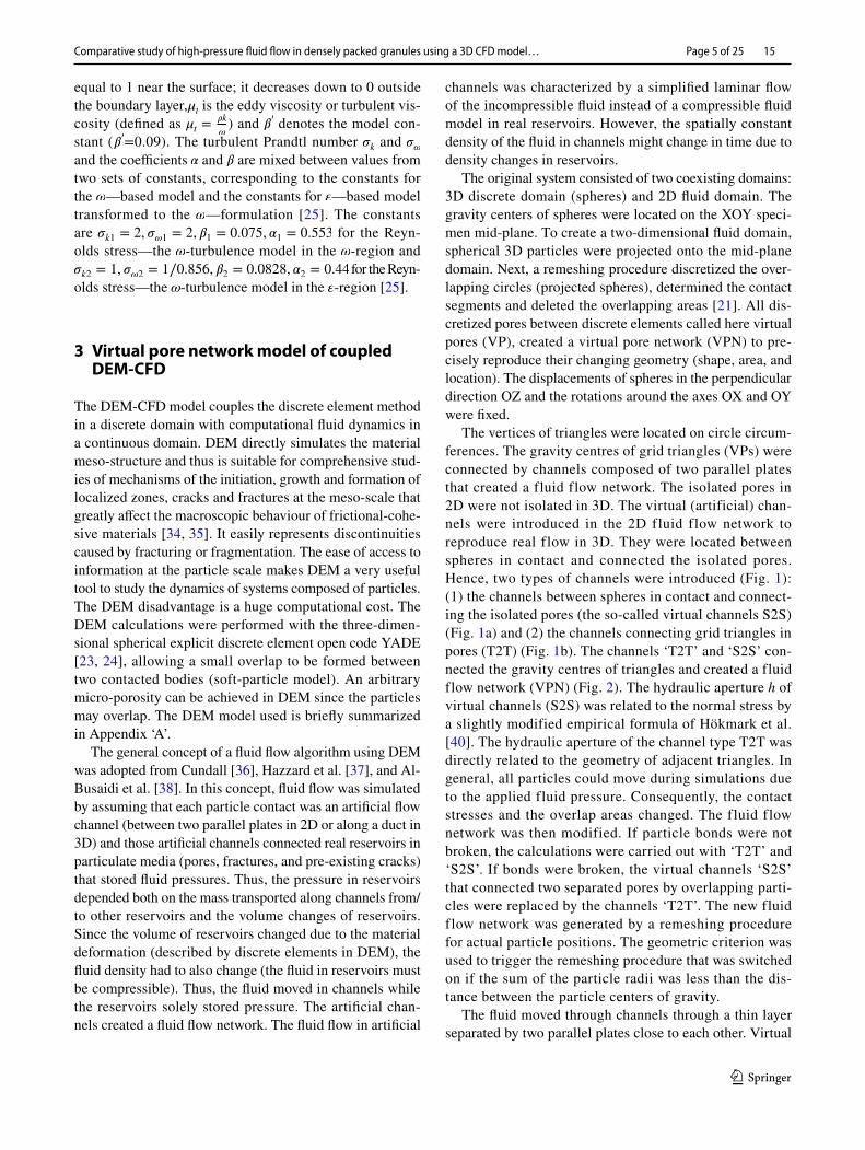
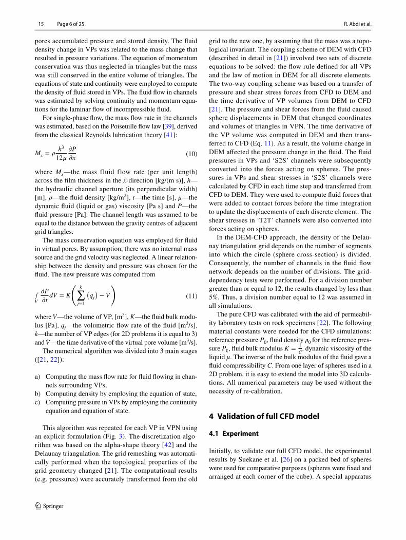
The vertices of triangles were located on circle circum-ferences. The gravity centres of grid triangles (VPs) were connected by channels composed of two parallel plates that created a fluid flow network. The isolated pores in 2D were not isolated in 3D. The virtual (artificial) chan-nels were introduced in the 2D fluid flow network to reproduce real flow in 3D. They were located between spheres in contact and connected the isolated pores. Hence, two types of channels were introduced (Fig. 1): (1) the channels between spheres in contact and connect-ing the isolated pores (the so-called virtual channels S2S) (Fig. 1a) and (2) the channels connecting grid triangles in pores (T2T) (Fig. 1b). The channels ‘T2T’ and ‘S2S’ con-nected the gravity centres of triangles and created a fluid flow network (VPN) (Fig. 2). The hydraulic aperture h of virtual channels (S2S) was related to the normal stress by a slightly modified empirical formula of Hökmark et al. [40]. The hydraulic aperture of the channel type T2T was directly related to the geometry of adjacent triangles. In general, all particles could move during simulations due to the applied fluid pressure. Consequently, the contact stresses and the overlap areas changed. The fluid flow network was then modified. If particle bonds were not broken, the calculations were carried out with ‘T2T’ and ‘S2S’. If bonds were broken, the virtual channels ‘S2S’ that connected two separated pores by overlapping parti-cles were replaced by the channels ‘T2T’. The new fluid flow network was generated by a remeshing procedure for actual particle positions. The geometric criterion was used to trigger the remeshing procedure that was switched on if the sum of the particle radii was less than the dis-tance between the particle centers of gravity.

The fluid moved through channels through a thin layer separated by two parallel plates close to each other. Virtual

R. Abdi et al.

1 3

15 Page 6 of 25

pores accumulated pressure and stored density. The fluid density change in VPs was related to the mass change that resulted in pressure variations. The equation of momentum conservation was thus neglected in triangles but the mass was still conserved in the entire volume of triangles. The equations of state and continuity were employed to compute the density of fluid stored in VPs. The fluid flow in channels was estimated by solving continuity and momentum equa-tions for the laminar flow of incompressible fluid.

For single-phase flow, the mass flow rate in the channels was estimated, based on the Poiseuille flow law [39], derived from the classical Reynolds lubrication theory [41]:

where Mx—the mass fluid flow rate (per unit length) across the film thickness in the x-direction [kg/(m s)], h—the hydraulic channel aperture (its perpendicular width) [m], ρ—the fluid density [kg/m3], t—the time [s], μ—the dynamic fluid (liquid or gas) viscosity [Pa s] and P—the fluid pressure [Pa]. The channel length was assumed to be equal to the distance between the gravity centres of adjacent grid triangles.

The mass conservation equation was employed for fluid in virtual pores. By assumption, there was no internal mass source and the grid velocity was neglected. A linear relation-ship between the density and pressure was chosen for the fluid. The new pressure was computed from

where V—the volume of VP, [m3], K—the fluid bulk modu-lus [Pa], qj—the volumetric flow rate of the fluid [m3/s], k—the number of VP edges (for 2D problems it is equal to 3) and V—the time derivative of the virtual pore volume [m3/s].

The numerical algorithm was divided into 3 main stages ([21, 22]):

a) Computing the mass flow rate for fluid flowing in chan-nels surrounding VPs,

b) Computing density by employing the equation of state,c) Computing pressure in VPs by employing the continuity

equation and equation of state.

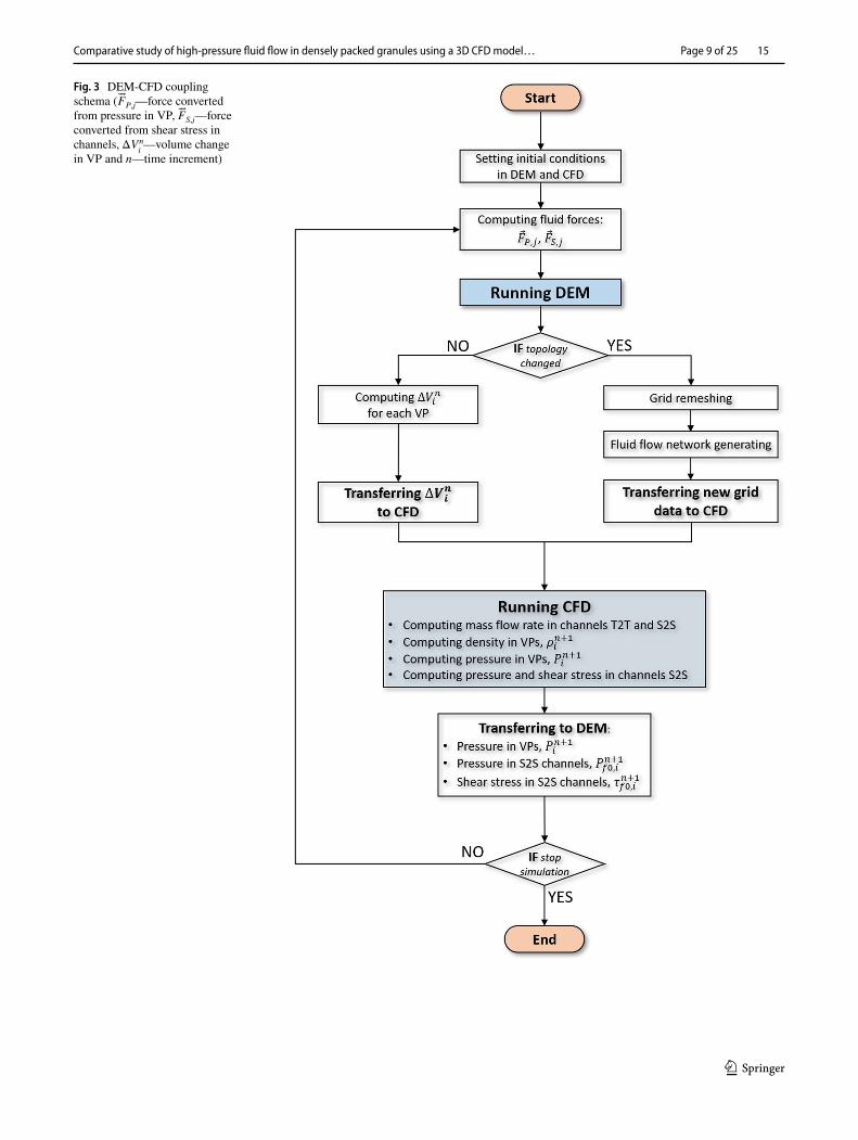
This algorithm was repeated for each VP in VPN using an explicit formulation (Fig. 3). The discretization algo-rithm was based on the alpha-shape theory [42] and the Delaunay triangulation. The grid remeshing was automati-cally performed when the topological properties of the grid geometry changed [21]. The computational results (e.g. pressures) were accurately transformed from the old

(10)Mx = �h3

12�

�P

�x

(11)∫V

𝜕P

𝜕tdV = K

(

k∑

j=1

(

qj)

− V

)

grid to the new one, by assuming that the mass was a topo-logical invariant. The coupling scheme of DEM with CFD (described in detail in [21]) involved two sets of discrete equations to be solved: the flow rule defined for all VPs and the law of motion in DEM for all discrete elements. The two-way coupling scheme was based on a transfer of pressure and shear stress forces from CFD to DEM and the time derivative of VP volumes from DEM to CFD [21]. The pressure and shear forces from the fluid caused sphere displacements in DEM that changed coordinates and volumes of triangles in VPN. The time derivative of the VP volume was computed in DEM and then trans-ferred to CFD (Eq. 11). As a result, the volume change in DEM affected the pressure change in the fluid. The fluid pressures in VPs and ‘S2S’ channels were subsequently converted into the forces acting on spheres. The pres-sures in VPs and shear stresses in ‘S2S’ channels were calculated by CFD in each time step and transferred from CFD to DEM. They were used to compute fluid forces that were added to contact forces before the time integration to update the displacements of each discrete element. The shear stresses in ‘T2T’ channels were also converted into forces acting on spheres.

In the DEM-CFD approach, the density of the Delau-nay triangulation grid depends on the number of segments into which the circle (sphere cross-section) is divided. Consequently, the number of channels in the fluid flow network depends on the number of divisions. The grid-dependency tests were performed. For a division number greater than or equal to 12, the results changed by less than 5%. Thus, a division number equal to 12 was assumed in all simulations.

The pure CFD was calibrated with the aid of permeabil-ity laboratory tests on rock specimens [22]. The following material constants were needed for the CFD simulations: reference pressure P0 , fluid density �0 for the reference pres-sure P0 , fluid bulk modulus K =

1

C , dynamic viscosity of the

liquid μ. The inverse of the bulk modulus of the fluid gave a fluid compressibility C. From one layer of spheres used in a 2D problem, it is easy to extend the model into 3D calcula-tions. All numerical parameters may be used without the necessity of re-calibration.

4 Validation of full CFD model

4.1 Experiment

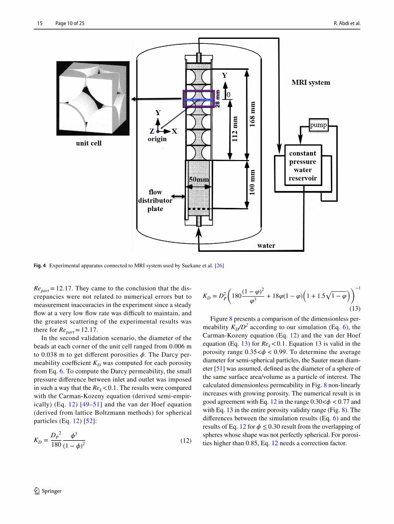
Initially, to validate our full CFD model, the experimental results by Suekane et al. [26] on a packed bed of spheres were used for comparative purposes (spheres were fixed and arranged at each corner of the cube). A special apparatus


1 3

Page 7 of 25 15

was constructed to measure the velocities of the fluid propa-gating through voids of a packed specimen (Fig. 4). The velocities were measured with the magnetic resonance imag-ing (MRI) technique. The experimental apparatus included a flow channel aligned vertically inside the MRI system.

The diameter of the channel was d = 50 mm. The fluid chan-nel was composed of 5 unit cells of the same size. Each unit cell 28 × 28 × 28 mm3 had a cubic shape and contained eight fixed 1/8 spheres with a diameter DP = 28 mm. The spheres were placed in two layers with four 1/8 spheres. The

Fig. 1 Fluid flow network in rock matrix with triangular dis-cretization of pores (in blue): A channel type ‘S2S’ (red colour) and B channel type ‘T2T’ (red colour) [21, 22]

Fig. 2 Fluid flow network in rock matrix (A—zoomed area)

R. Abdi et al.

1 3

15 Page 8 of 25

volumetric porosity ϕ of the unit cell was ϕ = 47.6%. The circulating fluid was water supplied from a reservoir with a constant pressure to keep the flow rate constant. Three components of the fluid velocity vectors in the 3D void space were directly visualized. The y-component of the fluid veloc-ity was registered in the fourth unit cell at y = 0 (Fig. 4) for five different Repart numbers from the inertial flow region to the unsteady laminar flow region. The velocities were presented along the x-axis (blue line in Fig. 4). The phase encoding method was used [43] to find the velocity distri-bution in a specimen cross-section. The Reynolds numbers Repart for the streamwise velocity for five arbitrarily chosen particles were: 12.17, 28.88, 59.78, 105.5, and 204.74. The dominant flow regime for Repart = 204.74 was reported to be laminar ([27, 44–46]).

For the value of Repart = 12.17, the fluid velocity decreased with the increasing area of cross-section normal to the main flow direction (the local geometry significantly influenced the flow). The water flowed over the surfaces of spheres like a creeping flow in which viscous forces were dominant. When increasing Repart, the local geometry was not the only factor affecting the velocity variation due to an increasing influence of inertia forces over viscous forces. With the high value of Repart (e.g. 204.74), where the inertial forces were dominant, the fluid moved through the pores like a jet without a velocity change. The maximum velocity in the center of pores increased with a growth of Repart even four times as compared to the average velocity in pores. The velocity profile was always parabolic.

4.2 Numerical results

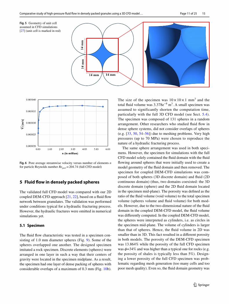
Our numerical results were also compared with similar numerical simulations of the experiment [26] performed by Gunjal et al. [27] with the commercial software ANSYS Fluent. Unstructured tetrahedral grids were assumed in their study to simulate incompressible laminar flow through a packed bed of fixed spheres [27]. A turbulent regime with the standard k-� model for the Repart numbers between 1000 and 2000 was considered in their study. The model was used to study fluid flow over a wide range of particle Reynolds numbers (12-2000) for different packing arrangements. A unit cell (in red colour in Fig. 5) was composed of eight 1/8 spheres. Translational periodic boundary conditions were assumed with the pressure drop to be periodic at all unit cell faces. A semi-implicit method for a pressure-linked equation (SIMPLE) algorithm was used for correcting a pressure gra-dient based on the difference between the target mass flow rate and the actual one. Symmetry boundary conditions were imposed on all vertical faces bounding the fluid domain. The velocity and all gradients normal to the faces were set to zero. No-slip boundary conditions were applied on the surfaces of spheres [27].

In our simulation on lateral surfaces of the specimen, symmetry boundary conditions were chosen with the veloc-ity normal to the surface, and all other normal gradients were set to zero. The velocity component parallel to the wall was computed only. In the inlet and outlet, periodic boundary conditions with a defined mass flow rate were chosen. On the sphere surfaces, no-slip conditions were defined where the fluid velocity was set to zero. The water entered the inlet at 70 ℃. The properties of water (with a proppant) were as follows: the dynamic viscosity 0.000406 Pa·s and the density 977.36 kg/m3. An unstructured tetrahedral mesh was also used to discretize the fluid domain. A very dense mesh was assumed in the vicinity of spheres, to capture high-velocity gradients and related high shear stresses. The mesh depend-ency test was carried out by measuring the pore average streamwise velocity Vy in the unit cell against the number of elements (Fig. 6). The streamwise velocity converged for the number of elements greater than one million (Fig. 6) and the mesh setting corresponding to one million elements was adopted for simulations.

Two numerical validation scenarios were considered on the cubic experiment specimen composed of eight 1/8-spheres with a diameter of 28 mm diameters (Fig. 5). The first scenario compared the calculated fluid velocities with the experimental [26] and the numerical results [27]. The second scenario compared the permeability results using the two most common equations: Carman-Kozeny (Eq. 12) and van der Hoef (Eq. 13). FVM was adopted to solve governing equations. The discrete system of line-arized equations was solved using the algebraic multi-grid method by means of the incomplete lower upper (ILU) factorization technique. Hydrodynamic equations for u, v, w and p were solved as a single system by a coupled solver of ANSYS CFX [25]. A high-resolution scheme was used for the advection term. Pressure and velocity were coupled with a high-resolution scheme derived from the discretization algorithm developed by Rhie and Chow [47] and modified by Majumdar [48].

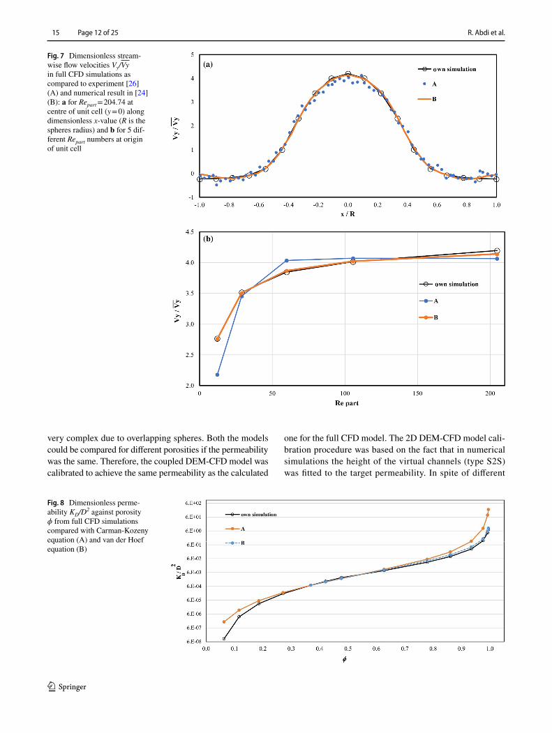
Figure 7a presents the dimensionless y-component of fluid velocities for Repart = 204.74 at y = 0 along the dimen-sionless x-value (blue line in Fig. 4). The distribution of the dimensionless y-component of velocity was parabolic and matched well with both the experimental [26] and numerical ones [27]. The dimensionless y-component of the fluid velocity at the center of the unit cell for five different values of the particle Reynolds number Repart is shown in Fig. 7b. The velocity variations are parabolic with increasing Repart. Good accordance of our numeri-cal results with the experimental [26] and numerical ones [26] was obtained except for the result Repart = 12.17. Gun-jal et al. [26] discussed in detail the possible causes of discrepancies between the results obtained in the experi-ment and those obtained in numerical simulations with


1 3

Page 9 of 25 15

Fig. 3 DEM-CFD coupling schema ( �FP,j—force converted from pressure in VP, �FS,j—force converted from shear stress in channels, ΔVn

i—volume change

in VP and n—time increment)

R. Abdi et al.

1 3

15 Page 10 of 25

Repart = 12.17. They came to the conclusion that the dis-crepancies were not related to numerical errors but to measurement inaccuracies in the experiment since a steady flow at a very low flow rate was difficult to maintain, and the greatest scattering of the experimental results was there for Repart = 12.17.

In the second validation scenario, the diameter of the beads at each corner of the unit cell ranged from 0.006 m to 0.038 m to get different porosities ϕ. The Darcy per-meability coefficient KD was computed for each porosity from Eq. 6. To compute the Darcy permeability, the small pressure difference between inlet and outlet was imposed in such a way that the Rek < 0.1. The results were compared with the Carman-Kozeny equation (derived semi-empir-ically) (Eq. 12) [49–51] and the van der Hoef equation (derived from lattice Boltzmann methods) for spherical particles (Eq. 12) [52]:

(12)KD =DP

2

180

�3

(1 − �)2

Figure 8 presents a comparison of the dimensionless per-meability KD/D2 according to our simulation (Eq. 6), the Carman-Kozeny equation (Eq. 12) and the van der Hoef equation (Eq. 13) for Rek < 0.1. Equation 13 is valid in the porosity range 0.35<𝜙 < 0.99. To determine the average diameter for semi-spherical particles, the Sauter mean diam-eter [51] was assumed, defined as the diameter of a sphere of the same surface area/volume as a particle of interest. The calculated dimensionless permeability in Fig. 8 non-linearly increases with growing porosity. The numerical result is in good agreement with Eq. 12 in the range 0.30<𝜙 < 0.77 and with Eq. 13 in the entire porosity validity range (Fig. 8). The differences between the simulation results (Eq. 6) and the results of Eq. 12 for � ≤ 0.30 result from the overlapping of spheres whose shape was not perfectly spherical. For porosi-ties higher than 0.85, Eq. 12 needs a correction factor.

(13)

KD = D2P

�

180(1 − �)2

�3+ 18�(1 − �)

�

1 + 1.5√

1 − ��

�−1

Fig. 4 Experimental apparatus connected to MRI system used by Suekane et al. [26]


1 3

Page 11 of 25 15

5 Fluid flow in densely packed spheres

The validated full CFD model was compared with our 2D coupled DEM-CFD approach [21, 22], based on a fluid flow network between granulates. The validation was performed under conditions typical for a hydraulic fracturing process. However, the hydraulic fractures were omitted in numerical simulations yet.

5.1 Specimen

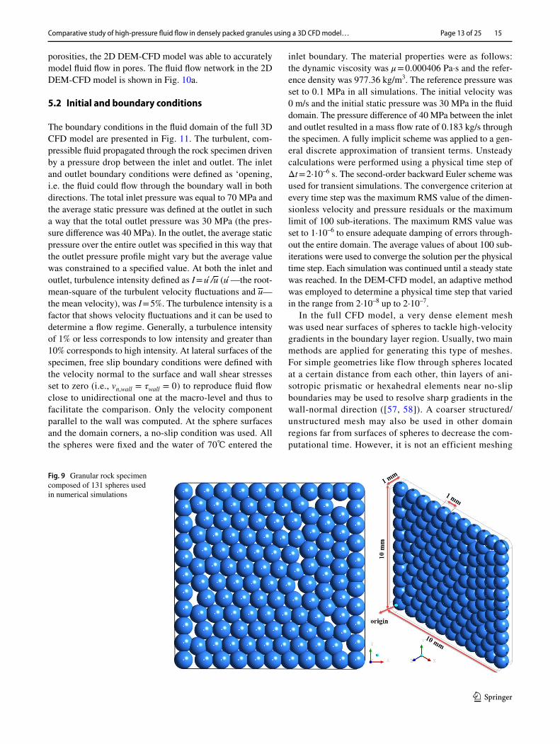
The fluid flow characteristic was tested in a specimen con-sisting of 1.0 mm diameter spheres (Fig. 9). Some of the spheres overlapped one another. The designed specimen imitated a rock specimen. Discrete elements (spheres) were arranged in one layer in such a way that their centers of gravity were located in the specimen midplane. As a result, the specimen had one layer of dense packing of spheres with considerable overlaps of a maximum of 0.3 mm (Fig. 10b).

The size of the specimen was 10 × 10 × 1 mm3 and the total fluid volume was 3.378e−8 m3. A small specimen was assumed to significantly shorten the computation time, particularly with the full 3D CFD model (see Sect. 5.4). The specimen was composed of 131 spheres in a random arrangement. Other researchers who studied fluid flow in dense sphere systems, did not consider overlaps of spheres (e.g. [33, 50, 54–56]) due to meshing problems. Very high pressures (up to 70 MPa) were chosen to reproduce the nature of a hydraulic fracturing process.

The same sphere arrangement was used in both speci-mens. However, the specimen for simulations with the full CFD model solely contained the fluid domain with the fluid flowing around spheres that were initially used to create a model geometry of the fluid domain and then removed. The specimen for coupled DEM-CFD simulations was com-posed of both spheres (3D discrete domain) and fluid (2D continuous domain) (thus, two domains coexisted: the 3D discrete domain (sphere) and the 2D fluid domain located in the specimen mid-plane). The porosity was defined as the ratio of the fluid volume (void volume) to the total specimen volume (spheres volume and fluid volume) for both mod-els. However, due to the two-dimensional nature of the fluid domain in the coupled DEM-CFD model, the fluid volume was differently computed. In the coupled DEM-CFD model, the spheres were interpreted as cylinders, i.e. as circles in the specimen mid-plane. The volume of cylinders is larger than that of spheres. Hence, the fluid volume in 2D was smaller than in 3D. This fact resulted in a different porosity in both models. The porosity of the DEM-CFD specimen was 13.864% while the porosity of the full CFD specimen was �=34% and was higher than a typical one for rocks (e.g. the porosity of shales is typically less than 5%). Design-ing a lower porosity of the full CFD specimen was prob-lematic regarding mesh generation (too many cells and too poor mesh quality). Even so, the fluid domain geometry was

Fig. 5 Geometry of unit cell assumed in CFD simulations [27] (unit cell is marked in red)

Fig. 6 Pore average streamwise velocity versus number of elements n for particle Reynolds number Repart = 204.74 (full CFD model)

R. Abdi et al.

1 3

15 Page 12 of 25

very complex due to overlapping spheres. Both the models could be compared for different porosities if the permeability was the same. Therefore, the coupled DEM-CFD model was calibrated to achieve the same permeability as the calculated

one for the full CFD model. The 2D DEM-CFD model cali-bration procedure was based on the fact that in numerical simulations the height of the virtual channels (type S2S) was fitted to the target permeability. In spite of different

Fig. 7 Dimensionless stream-wise flow velocities Vy/Vy in full CFD simulations as compared to experiment [26] (A) and numerical result in [24] (B): a for Repart = 204.74 at centre of unit cell (y = 0) along dimensionless x-value (R is the spheres radius) and b for 5 dif-ferent Repart numbers at origin of unit cell

Fig. 8 Dimensionless perme-ability KD/D2 against porosity ϕ from full CFD simulations compared with Carman-Kozeny equation (A) and van der Hoef equation (B)


1 3

Page 13 of 25 15

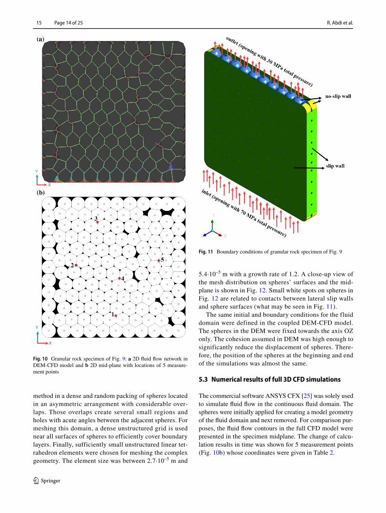
porosities, the 2D DEM-CFD model was able to accurately model fluid flow in pores. The fluid flow network in the 2D DEM-CFD model is shown in Fig. 10a.

5.2 Initial and boundary conditions

The boundary conditions in the fluid domain of the full 3D CFD model are presented in Fig. 11. The turbulent, com-pressible fluid propagated through the rock specimen driven by a pressure drop between the inlet and outlet. The inlet and outlet boundary conditions were defined as ‘opening, i.e. the fluid could flow through the boundary wall in both directions. The total inlet pressure was equal to 70 MPa and the average static pressure was defined at the outlet in such a way that the total outlet pressure was 30 MPa (the pres-sure difference was 40 MPa). In the outlet, the average static pressure over the entire outlet was specified in this way that the outlet pressure profile might vary but the average value was constrained to a specified value. At both the inlet and outlet, turbulence intensity defined as I = u /u (u —the root-mean-square of the turbulent velocity fluctuations and u—the mean velocity), was I = 5%. The turbulence intensity is a factor that shows velocity fluctuations and it can be used to determine a flow regime. Generally, a turbulence intensity of 1% or less corresponds to low intensity and greater than 10% corresponds to high intensity. At lateral surfaces of the specimen, free slip boundary conditions were defined with the velocity normal to the surface and wall shear stresses set to zero (i.e., vn,wall = �wall = 0 ) to reproduce fluid flow close to unidirectional one at the macro-level and thus to facilitate the comparison. Only the velocity component parallel to the wall was computed. At the sphere surfaces and the domain corners, a no-slip condition was used. All the spheres were fixed and the water of 70℃ entered the

inlet boundary. The material properties were as follows: the dynamic viscosity was μ = 0.000406 Pa·s and the refer-ence density was 977.36 kg/m3. The reference pressure was set to 0.1 MPa in all simulations. The initial velocity was 0 m/s and the initial static pressure was 30 MPa in the fluid domain. The pressure difference of 40 MPa between the inlet and outlet resulted in a mass flow rate of 0.183 kg/s through the specimen. A fully implicit scheme was applied to a gen-eral discrete approximation of transient terms. Unsteady calculations were performed using a physical time step of Δt = 2·10–6 s. The second-order backward Euler scheme was used for transient simulations. The convergence criterion at every time step was the maximum RMS value of the dimen-sionless velocity and pressure residuals or the maximum limit of 100 sub-iterations. The maximum RMS value was set to 1·10–6 to ensure adequate damping of errors through-out the entire domain. The average values of about 100 sub-iterations were used to converge the solution per the physical time step. Each simulation was continued until a steady state was reached. In the DEM-CFD model, an adaptive method was employed to determine a physical time step that varied in the range from 2·10–8 up to 2·10–7.

In the full CFD model, a very dense element mesh was used near surfaces of spheres to tackle high-velocity gradients in the boundary layer region. Usually, two main methods are applied for generating this type of meshes. For simple geometries like flow through spheres located at a certain distance from each other, thin layers of ani-sotropic prismatic or hexahedral elements near no-slip boundaries may be used to resolve sharp gradients in the wall-normal direction ([57, 58]). A coarser structured/unstructured mesh may also be used in other domain regions far from surfaces of spheres to decrease the com-putational time. However, it is not an efficient meshing

Fig. 9 Granular rock specimen composed of 131 spheres used in numerical simulations

R. Abdi et al.

1 3

15 Page 14 of 25

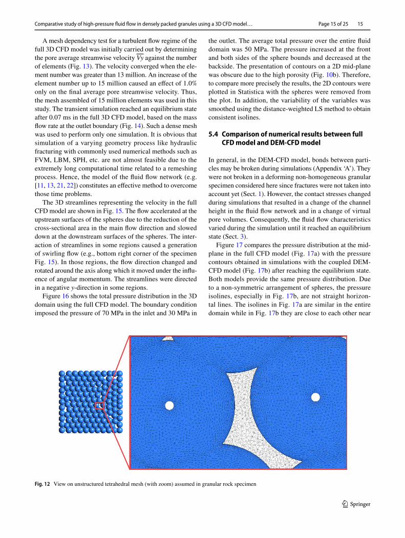
method in a dense and random packing of spheres located in an asymmetric arrangement with considerable over-laps. Those overlaps create several small regions and holes with acute angles between the adjacent spheres. For meshing this domain, a dense unstructured grid is used near all surfaces of spheres to efficiently cover boundary layers. Finally, sufficiently small unstructured linear tet-rahedron elements were chosen for meshing the complex geometry. The element size was between 2.7·10–5 m and

5.4·10–5 m with a growth rate of 1.2. A close-up view of the mesh distribution on spheres’ surfaces and the mid-plane is shown in Fig. 12. Small white spots on spheres in Fig. 12 are related to contacts between lateral slip walls and sphere surfaces (what may be seen in Fig. 11).

The same initial and boundary conditions for the fluid domain were defined in the coupled DEM-CFD model. The spheres in the DEM were fixed towards the axis OZ only. The cohesion assumed in DEM was high enough to significantly reduce the displacement of spheres. There-fore, the position of the spheres at the beginning and end of the simulations was almost the same.

5.3 Numerical results of full 3D CFD simulations

The commercial software ANSYS CFX [25] was solely used to simulate fluid flow in the continuous fluid domain. The spheres were initially applied for creating a model geometry of the fluid domain and next removed. For comparison pur-poses, the fluid flow contours in the full CFD model were presented in the specimen midplane. The change of calcu-lation results in time was shown for 5 measurement points (Fig. 10b) whose coordinates were given in Table 2.

Fig. 10 Granular rock specimen of Fig. 9: a 2D fluid flow network in DEM-CFD model and b 2D mid-plane with locations of 5 measure-ment points

Fig. 11 Boundary conditions of granular rock specimen of Fig. 9


1 3

Page 15 of 25 15

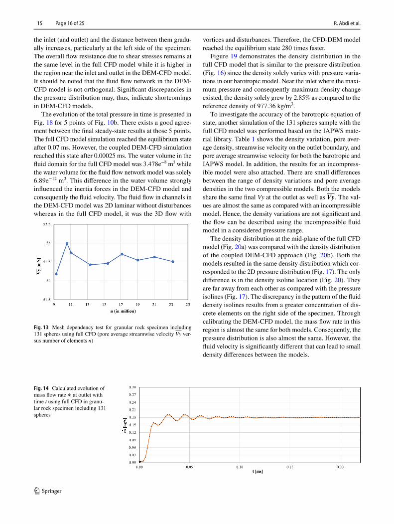
A mesh dependency test for a turbulent flow regime of the full 3D CFD model was initially carried out by determining the pore average streamwise velocity Vy against the number of elements (Fig. 13). The velocity converged when the ele-ment number was greater than 13 million. An increase of the element number up to 15 million caused an effect of 1.0% only on the final average pore streamwise velocity. Thus, the mesh assembled of 15 million elements was used in this study. The transient simulation reached an equilibrium state after 0.07 ms in the full 3D CFD model, based on the mass flow rate at the outlet boundary (Fig. 14). Such a dense mesh was used to perform only one simulation. It is obvious that simulation of a varying geometry process like hydraulic fracturing with commonly used numerical methods such as FVM, LBM, SPH, etc. are not almost feasible due to the extremely long computational time related to a remeshing process. Hence, the model of the fluid flow network (e.g. [11, 13, 21, 22]) constitutes an effective method to overcome those time problems.

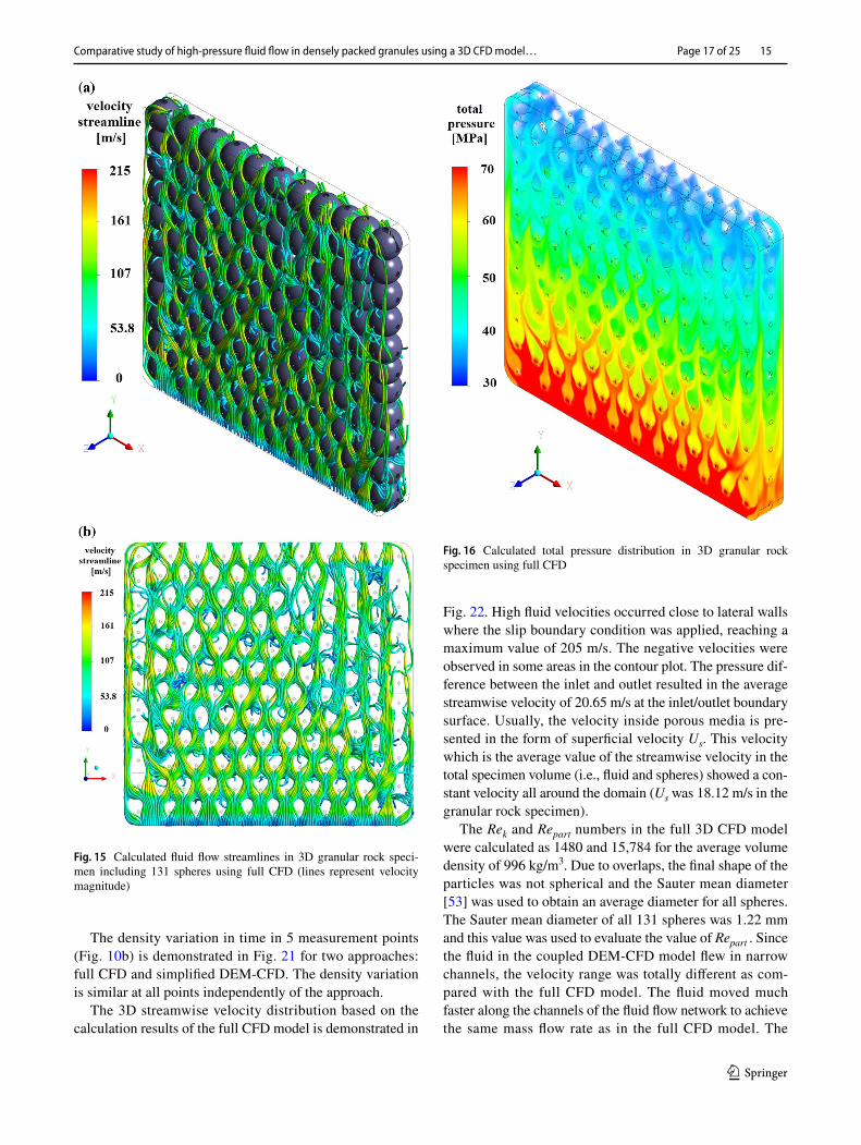
The 3D streamlines representing the velocity in the full CFD model are shown in Fig. 15. The flow accelerated at the upstream surfaces of the spheres due to the reduction of the cross-sectional area in the main flow direction and slowed down at the downstream surfaces of the spheres. The inter-action of streamlines in some regions caused a generation of swirling flow (e.g., bottom right corner of the specimen Fig. 15). In those regions, the flow direction changed and rotated around the axis along which it moved under the influ-ence of angular momentum. The streamlines were directed in a negative y-direction in some regions.

Figure 16 shows the total pressure distribution in the 3D domain using the full CFD model. The boundary condition imposed the pressure of 70 MPa in the inlet and 30 MPa in

the outlet. The average total pressure over the entire fluid domain was 50 MPa. The pressure increased at the front and both sides of the sphere bounds and decreased at the backside. The presentation of contours on a 2D mid-plane was obscure due to the high porosity (Fig. 10b). Therefore, to compare more precisely the results, the 2D contours were plotted in Statistica with the spheres were removed from the plot. In addition, the variability of the variables was smoothed using the distance-weighted LS method to obtain consistent isolines.

5.4 Comparison of numerical results between full CFD model and DEM‑CFD model

In general, in the DEM-CFD model, bonds between parti-cles may be broken during simulations (Appendix ‘A’). They were not broken in a deforming non-homogeneous granular specimen considered here since fractures were not taken into account yet (Sect. 1). However, the contact stresses changed during simulations that resulted in a change of the channel height in the fluid flow network and in a change of virtual pore volumes. Consequently, the fluid flow characteristics varied during the simulation until it reached an equilibrium state (Sect. 3).

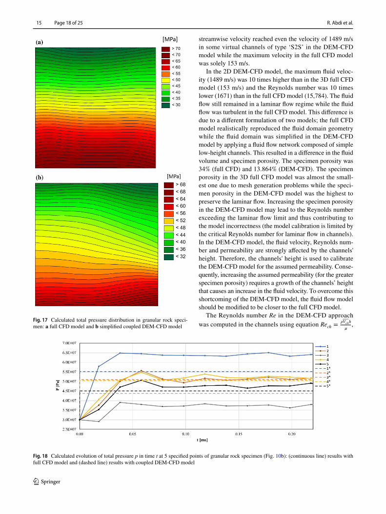
Figure 17 compares the pressure distribution at the mid-plane in the full CFD model (Fig. 17a) with the pressure contours obtained in simulations with the coupled DEM-CFD model (Fig. 17b) after reaching the equilibrium state. Both models provide the same pressure distribution. Due to a non-symmetric arrangement of spheres, the pressure isolines, especially in Fig. 17b, are not straight horizon-tal lines. The isolines in Fig. 17a are similar in the entire domain while in Fig. 17b they are close to each other near

Fig. 12 View on unstructured tetrahedral mesh (with zoom) assumed in granular rock specimen

R. Abdi et al.

1 3

15 Page 16 of 25

the inlet (and outlet) and the distance between them gradu-ally increases, particularly at the left side of the specimen. The overall flow resistance due to shear stresses remains at the same level in the full CFD model while it is higher in the region near the inlet and outlet in the DEM-CFD model. It should be noted that the fluid flow network in the DEM-CFD model is not orthogonal. Significant discrepancies in the pressure distribution may, thus, indicate shortcomings in DEM-CFD models.

The evolution of the total pressure in time is presented in Fig. 18 for 5 points of Fig. 10b. There exists a good agree-ment between the final steady-state results at those 5 points. The full CFD model simulation reached the equilibrium state after 0.07 ms. However, the coupled DEM-CFD simulation reached this state after 0.00025 ms. The water volume in the fluid domain for the full CFD model was 3.478e−8 m3 while the water volume for the fluid flow network model was solely 6.89e−12 m3. This difference in the water volume strongly influenced the inertia forces in the DEM-CFD model and consequently the fluid velocity. The fluid flow in channels in the DEM-CFD model was 2D laminar without disturbances whereas in the full CFD model, it was the 3D flow with

vortices and disturbances. Therefore, the CFD-DEM model reached the equilibrium state 280 times faster.

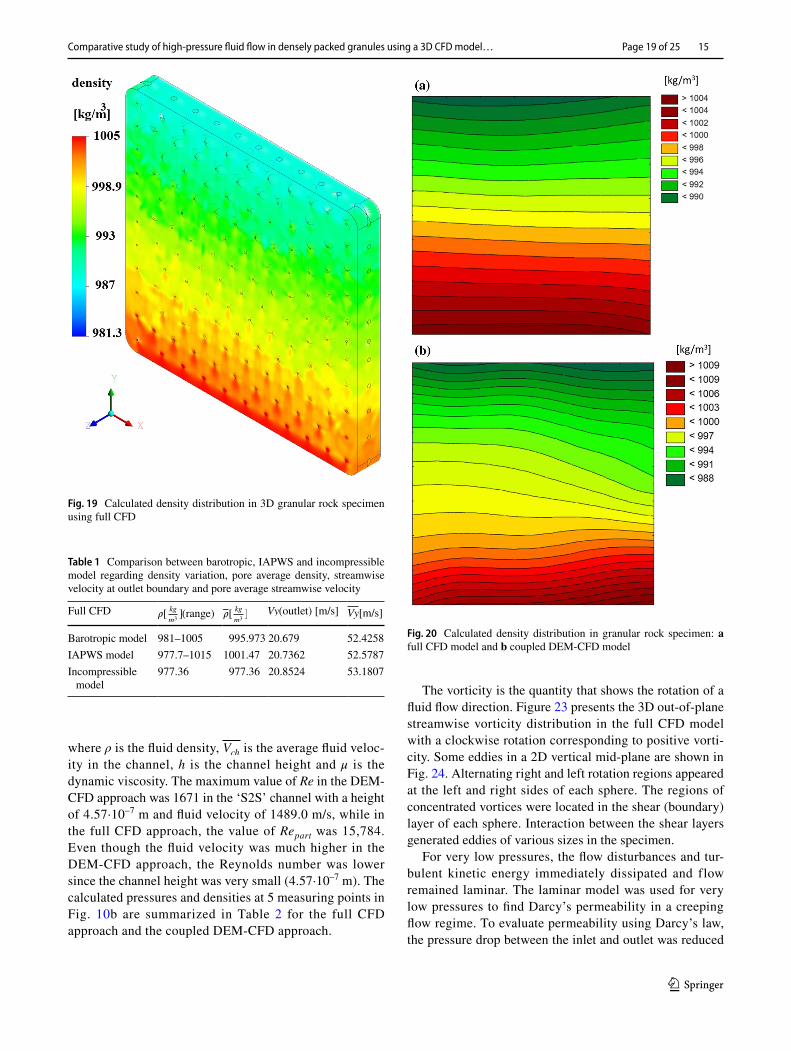
Figure 19 demonstrates the density distribution in the full CFD model that is similar to the pressure distribution (Fig. 16) since the density solely varies with pressure varia-tions in our barotropic model. Near the inlet where the maxi-mum pressure and consequently maximum density change existed, the density solely grew by 2.85% as compared to the reference density of 977.36 kg/m3.

To investigate the accuracy of the barotropic equation of state, another simulation of the 131 spheres sample with the full CFD model was performed based on the IAPWS mate-rial library. Table 1 shows the density variation, pore aver-age density, streamwise velocity on the outlet boundary, and pore average streamwise velocity for both the barotropic and IAPWS model. In addition, the results for an incompress-ible model were also attached. There are small differences between the range of density variations and pore average densities in the two compressible models. Both the models share the same final Vy at the outlet as well as Vy . The val-ues are almost the same as compared with an incompressible model. Hence, the density variations are not significant and the flow can be described using the incompressible fluid model in a considered pressure range.

The density distribution at the mid-plane of the full CFD model (Fig. 20a) was compared with the density distribution of the coupled DEM-CFD approach (Fig. 20b). Both the models resulted in the same density distribution which cor-responded to the 2D pressure distribution (Fig. 17). The only difference is in the density isoline location (Fig. 20). They are far away from each other as compared with the pressure isolines (Fig. 17). The discrepancy in the pattern of the fluid density isolines results from a greater concentration of dis-crete elements on the right side of the specimen. Through calibrating the DEM-CFD model, the mass flow rate in this region is almost the same for both models. Consequently, the pressure distribution is also almost the same. However, the fluid velocity is significantly different that can lead to small density differences between the models.

Fig. 13 Mesh dependency test for granular rock specimen including 131 spheres using full CFD (pore average streamwise velocity Vy ver-sus number of elements n)

Fig. 14 Calculated evolution of mass flow rate m at outlet with time t using full CFD in granu-lar rock specimen including 131 spheres


1 3

Page 17 of 25 15

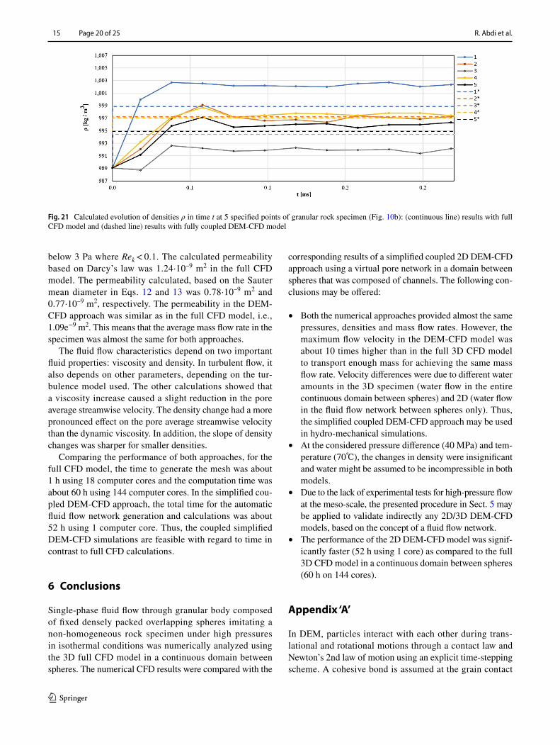
The density variation in time in 5 measurement points (Fig. 10b) is demonstrated in Fig. 21 for two approaches: full CFD and simplified DEM-CFD. The density variation is similar at all points independently of the approach.

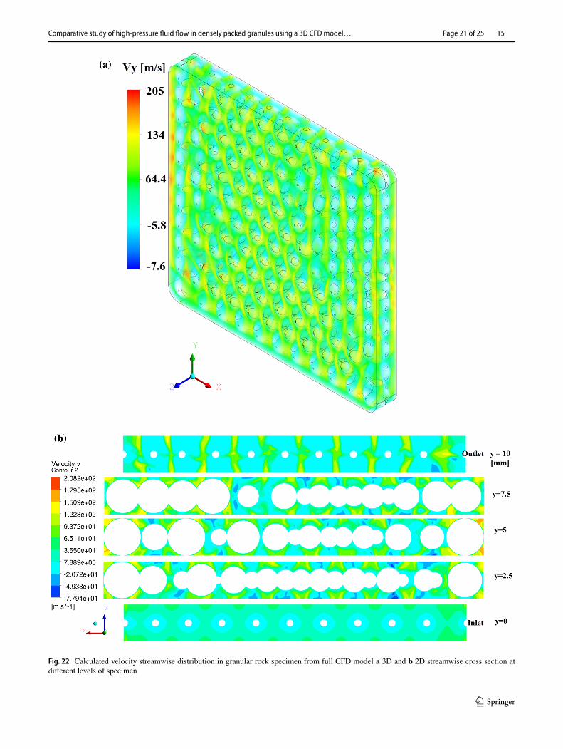
The 3D streamwise velocity distribution based on the calculation results of the full CFD model is demonstrated in

Fig. 22. High fluid velocities occurred close to lateral walls where the slip boundary condition was applied, reaching a maximum value of 205 m/s. The negative velocities were observed in some areas in the contour plot. The pressure dif-ference between the inlet and outlet resulted in the average streamwise velocity of 20.65 m/s at the inlet/outlet boundary surface. Usually, the velocity inside porous media is pre-sented in the form of superficial velocity Us. This velocity which is the average value of the streamwise velocity in the total specimen volume (i.e., fluid and spheres) showed a con-stant velocity all around the domain (Us was 18.12 m/s in the granular rock specimen).

The Rek and Repart numbers in the full 3D CFD model were calculated as 1480 and 15,784 for the average volume density of 996 kg/m3. Due to overlaps, the final shape of the particles was not spherical and the Sauter mean diameter [53] was used to obtain an average diameter for all spheres. The Sauter mean diameter of all 131 spheres was 1.22 mm and this value was used to evaluate the value of Repart . Since the fluid in the coupled DEM-CFD model flew in narrow channels, the velocity range was totally different as com-pared with the full CFD model. The fluid moved much faster along the channels of the fluid flow network to achieve the same mass flow rate as in the full CFD model. The

Fig. 15 Calculated fluid flow streamlines in 3D granular rock speci-men including 131 spheres using full CFD (lines represent velocity magnitude)

Fig. 16 Calculated total pressure distribution in 3D granular rock specimen using full CFD

R. Abdi et al.

1 3

15 Page 18 of 25

streamwise velocity reached even the velocity of 1489 m/s in some virtual channels of type ‘S2S’ in the DEM-CFD model while the maximum velocity in the full CFD model was solely 153 m/s.

In the 2D DEM-CFD model, the maximum fluid veloc-ity (1489 m/s) was 10 times higher than in the 3D full CFD model (153 m/s) and the Reynolds number was 10 times lower (1671) than in the full CFD model (15,784). The fluid flow still remained in a laminar flow regime while the fluid flow was turbulent in the full CFD model. This difference is due to a different formulation of two models; the full CFD model realistically reproduced the fluid domain geometry while the fluid domain was simplified in the DEM-CFD model by applying a fluid flow network composed of simple low-height channels. This resulted in a difference in the fluid volume and specimen porosity. The specimen porosity was 34% (full CFD) and 13.864% (DEM-CFD). The specimen porosity in the 3D full CFD model was almost the small-est one due to mesh generation problems while the speci-men porosity in the DEM-CFD model was the highest to preserve the laminar flow. Increasing the specimen porosity in the DEM-CFD model may lead to the Reynolds number exceeding the laminar flow limit and thus contributing to the model incorrectness (the model calibration is limited by the critical Reynolds number for laminar flow in channels). In the DEM-CFD model, the fluid velocity, Reynolds num-ber and permeability are strongly affected by the channels' height. Therefore, the channels' height is used to calibrate the DEM-CFD model for the assumed permeability. Conse-quently, increasing the assumed permeability (for the greater specimen porosity) requires a growth of the channels’ height that causes an increase in the fluid velocity. To overcome this shortcoming of the DEM-CFD model, the fluid flow model should be modified to be closer to the full CFD model.

The Reynolds number Re in the DEM-CFD approach was computed in the channels using equation Rech =

�Vchh

� ,

Fig. 17 Calculated total pressure distribution in granular rock speci-men: a full CFD model and b simplified coupled DEM-CFD model

Fig. 18 Calculated evolution of total pressure p in time t at 5 specified points of granular rock specimen (Fig. 10b): (continuous line) results with full CFD model and (dashed line) results with coupled DEM-CFD model


1 3

Page 19 of 25 15

where ρ is the fluid density, Vch is the average fluid veloc-ity in the channel, h is the channel height and μ is the dynamic viscosity. The maximum value of Re in the DEM-CFD approach was 1671 in the ‘S2S’ channel with a height of 4.57·10–7 m and fluid velocity of 1489.0 m/s, while in the full CFD approach, the value of Repart was 15,784. Even though the fluid velocity was much higher in the DEM-CFD approach, the Reynolds number was lower since the channel height was very small (4.57·10–7 m). The calculated pressures and densities at 5 measuring points in Fig. 10b are summarized in Table 2 for the full CFD approach and the coupled DEM-CFD approach.

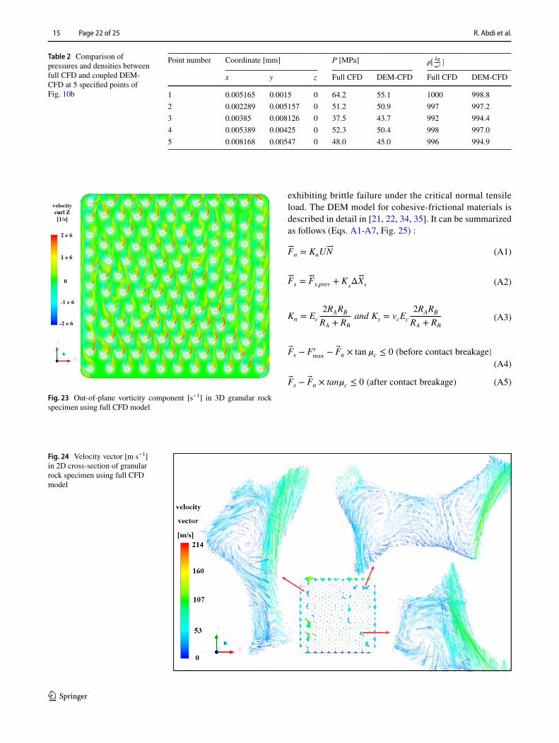
The vorticity is the quantity that shows the rotation of a fluid flow direction. Figure 23 presents the 3D out-of-plane streamwise vorticity distribution in the full CFD model with a clockwise rotation corresponding to positive vorti-city. Some eddies in a 2D vertical mid-plane are shown in Fig. 24. Alternating right and left rotation regions appeared at the left and right sides of each sphere. The regions of concentrated vortices were located in the shear (boundary) layer of each sphere. Interaction between the shear layers generated eddies of various sizes in the specimen.

For very low pressures, the flow disturbances and tur-bulent kinetic energy immediately dissipated and flow remained laminar. The laminar model was used for very low pressures to find Darcy’s permeability in a creeping flow regime. To evaluate permeability using Darcy’s law, the pressure drop between the inlet and outlet was reduced

Fig. 19 Calculated density distribution in 3D granular rock specimen using full CFD

Table 1 Comparison between barotropic, IAPWS and incompressible model regarding density variation, pore average density, streamwise velocity at outlet boundary and pore average streamwise velocity

Full CFD �[kg

m3](range) �[

kg

m3] Vy(outlet) [m/s] Vy[m/s]

Barotropic model 981–1005 995.973 20.679 52.4258IAPWS model 977.7–1015 1001.47 20.7362 52.5787Incompressible

model977.36 977.36 20.8524 53.1807

Fig. 20 Calculated density distribution in granular rock specimen: a full CFD model and b coupled DEM-CFD model

R. Abdi et al.

1 3

15 Page 20 of 25

below 3 Pa where Rek < 0.1. The calculated permeability based on Darcy’s law was 1.24·10–9 m2 in the full CFD model. The permeability calculated, based on the Sauter mean diameter in Eqs. 12 and 13 was 0.78·10–9 m2 and 0.77·10–9 m2, respectively. The permeability in the DEM-CFD approach was similar as in the full CFD model, i.e., 1.09e−9 m2. This means that the average mass flow rate in the specimen was almost the same for both approaches.

The fluid flow characteristics depend on two important fluid properties: viscosity and density. In turbulent flow, it also depends on other parameters, depending on the tur-bulence model used. The other calculations showed that a viscosity increase caused a slight reduction in the pore average streamwise velocity. The density change had a more pronounced effect on the pore average streamwise velocity than the dynamic viscosity. In addition, the slope of density changes was sharper for smaller densities.

Comparing the performance of both approaches, for the full CFD model, the time to generate the mesh was about 1 h using 18 computer cores and the computation time was about 60 h using 144 computer cores. In the simplified cou-pled DEM-CFD approach, the total time for the automatic fluid flow network generation and calculations was about 52 h using 1 computer core. Thus, the coupled simplified DEM-CFD simulations are feasible with regard to time in contrast to full CFD calculations.

6 Conclusions

Single-phase fluid flow through granular body composed of fixed densely packed overlapping spheres imitating a non-homogeneous rock specimen under high pressures in isothermal conditions was numerically analyzed using the 3D full CFD model in a continuous domain between spheres. The numerical CFD results were compared with the

corresponding results of a simplified coupled 2D DEM-CFD approach using a virtual pore network in a domain between spheres that was composed of channels. The following con-clusions may be offered:

• Both the numerical approaches provided almost the same pressures, densities and mass flow rates. However, the maximum flow velocity in the DEM-CFD model was about 10 times higher than in the full 3D CFD model to transport enough mass for achieving the same mass flow rate. Velocity differences were due to different water amounts in the 3D specimen (water flow in the entire continuous domain between spheres) and 2D (water flow in the fluid flow network between spheres only). Thus, the simplified coupled DEM-CFD approach may be used in hydro-mechanical simulations.

• At the considered pressure difference (40 MPa) and tem-perature (70℃), the changes in density were insignificant and water might be assumed to be incompressible in both models.

• Due to the lack of experimental tests for high-pressure flow at the meso-scale, the presented procedure in Sect. 5 may be applied to validate indirectly any 2D/3D DEM-CFD models, based on the concept of a fluid flow network.

• The performance of the 2D DEM-CFD model was signif-icantly faster (52 h using 1 core) as compared to the full 3D CFD model in a continuous domain between spheres (60 h on 144 cores).

Appendix ‘A’

In DEM, particles interact with each other during trans-lational and rotational motions through a contact law and Newton’s 2nd law of motion using an explicit time-stepping scheme. A cohesive bond is assumed at the grain contact

Fig. 21 Calculated evolution of densities ρ in time t at 5 specified points of granular rock specimen (Fig. 10b): (continuous line) results with full CFD model and (dashed line) results with fully coupled DEM-CFD model


1 3

Page 21 of 25 15

Fig. 22 Calculated velocity streamwise distribution in granular rock specimen from full CFD model a 3D and b 2D streamwise cross section at different levels of specimen

R. Abdi et al.

1 3

15 Page 22 of 25

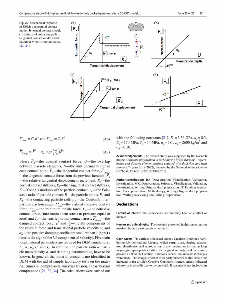
exhibiting brittle failure under the critical normal tensile load. The DEM model for cohesive-frictional materials is described in detail in [21, 22, 34, 35]. It can be summarized as follows (Eqs. A1-A7, Fig. 25) :

(A1)�Fn = KnU��N

(A2)�Fs =�Fs,prev + K

sΔ �Xs

(A3)Kn = Ec

2RARB

RA + RB

and Ks = vcEc

2RARB

RA + RB

(A4)Fs − Fs

max− Fn × tan𝜇c ≤ 0 (before contact breakage)

(A5)Fs − Fn × tan𝜇c ≤ 0 (after contact breakage)

Table 2 Comparison of pressures and densities between full CFD and coupled DEM-CFD at 5 specified points of Fig. 10b

Point number Coordinate [mm] P [MPa] �[kg

m3]

x y z Full CFD DEM-CFD Full CFD DEM-CFD

1 0.005165 0.0015 0 64.2 55.1 1000 998.82 0.002289 0.005157 0 51.2 50.9 997 997.23 0.00385 0.008126 0 37.5 43.7 992 994.44 0.005389 0.00425 0 52.3 50.4 998 997.05 0.008168 0.00547 0 48.0 45.0 996 994.9

Fig. 23 Out-of-plane vorticity component [s−1] in 3D granular rock specimen using full CFD model

Fig. 24 Velocity vector [m s−1] in 2D cross-section of granular rock specimen using full CFD model


1 3

Page 23 of 25 15

where �Fn—the normal contact force, U—the overlap between discrete elements, ��N—the unit normal vector at each contact point, �Fs—the tangential contact force, �Fs,prev

—the tangential contact force from the previous iteration, �Xs

—the relative tangential displacement increment, Kn—the normal contact stiffness, Ks—the tangential contact stiffness, Ec—Young’s modulus of the particle contact, νc—the Pois-son’s ratio of particle contact, R—the particle radius, RA and RB—the contacting particle radii μc—the Coulomb inter-particle friction angle, Fs

max—the critical cohesive contact

force, Fnmin

—the minimum tensile force, Cc—the cohesive contact stress (maximum shear stress at pressure equal to zero) and Tc—the tensile normal contact stress, �F

k

damp—the

damped contact force, �Fk and �vk

p—the kth components of

the residual force and translational particle velocity vp and αd—the positive damping coefficient smaller than 1 (sgn(•) returns the sign of the kth component of velocity). Five main local material parameters are required for DEM simulations: Ec, υc, μc, Cc and Tc. In addition, the particle radii R, parti-cle mass density ρc and damping parameters αd have to be known. In general, the material constants are identified in DEM with the aid of simple laboratory tests on the mate-rial (uniaxial compression, uniaxial tension, shear, biaxial compression) [21, 22, 34]. The calculations were carried out

(A6)Fsmax

= CcR2 and Fn

min= TcR

2

(A7)Fkdamp

= Fk − 𝛼d ⋅ sgn(

vkp

)

Fk

with the following constants [21]: Ec = 3.36 GPa, υc = 0.3, Cc = 170 MPa, Tc = 34 MPa, μc = 18°, ρc = 2600 kg/m3 and αd = 0.10.

Acknowledgements The present study was supported by the research project “Fracture propagation in rocks during hydro-fracking – experi-ments and discrete element method coupled with fluid flow and heat transport” (years 2019-2022), financed by the National Science Centre (NCN) (UMO-2018/29/B/ST8/00255).

Author contributions RA: Data curation, Visualization, Validation, Investigation. MK: Data curation, Software, Visualization, Validation, Investigation, Writing-Original draft preparation. JT: Funding acquisi-tion, Conceptualization, Methodology, Writing-Original draft prepara-tion, Writing-Reviewing and Editing, Supervision.

Declarations

Conflict of interest The authors declare that they have no conflict of interest.

Human and animal rights The research presented in this paper has not involved human participants or animals.

Open Access This article is licensed under a Creative Commons Attri-bution 4.0 International License, which permits use, sharing, adapta-tion, distribution and reproduction in any medium or format, as long as you give appropriate credit to the original author(s) and the source, provide a link to the Creative Commons licence, and indicate if changes were made. The images or other third party material in this article are included in the article's Creative Commons licence, unless indicated otherwise in a credit line to the material. If material is not included in

Fig. 25 Mechanical response of DEM: a tangential contact model, b normal contact model, c loading and unloading path in tangential contact model and d modified Mohr–Coulomb model [23, 24]

R. Abdi et al.

1 3

15 Page 24 of 25

the article's Creative Commons licence and your intended use is not permitted by statutory regulation or exceeds the permitted use, you will need to obtain permission directly from the copyright holder. To view a copy of this licence, visit http:// creat iveco mmons. org/ licen ses/ by/4. 0/.

References

1. Lathama, J., Munjiz, A., Mindel, J.: Modelling of massive par-ticulates for breakwater engineering using coupled FEM/DEM and CFD. Particuology 6, 572–583 (2008)

2. Zhao, J., Shan, T.: Coupled CFD–DEM simulation of fluid–parti-cle interaction in geomechanics. Powder Technol. 239, 248–258 (2013)

3. Shan, T., Zhao, J.: A coupled CFD-DEM analysis of granular flow impacting on a water reservoir. Acta Mech. 225(8), 2449–2470 (2014)

4. Zhou, F., Hu, S., Liu, Y., Liu, C., Xia, T.: CFD-DEM simulation of the pneumatic conveying of fine particles through a horizontal slit. Particuology 16, 196–205 (2014)

5. Wiese, J., Wissing, F., Höhner, D., Wirtz, S., Scherer, V., Ley, U., et al.: DEM/CFD modeling of the fuel conversion in a pellet stove. Fuel Process. Technol. 152, 223–239 (2016)

6. Ebrahimi, M., Crapper, M.: CFD-DEM simulation of turbulence modulation in horizontal pneumatic conveying. Particuology 31, 15–24 (2017)

7. Wissing, F., Wirtz, S., Scherer, V.: Simulating municipal solid waste incineration with a DEM/CFD method–influences of waste properties, grate and furnace design. Fuel 206, 638–656 (2017)

8. Yoon, J.S., Zang, A., Stephansson, O.: Numerical investigation on optimized stimulation of intact and naturally fractured deep geothermal reservoirs using hydro-mechanical coupled discrete particles joints model. Geothermics 52, 165–184 (2014)

9. Shimizu, H., Murata, S., Ishida, T.: The distinct element analysis for hydraulic fracturing in hard rock considering fluid viscosity and particle size distribution. Int. J. Rock Mech. Min. Sci. 48(5), 712–727 (2011)

10. Ma, X., Zhou, T., Zou, Y.: Experimental and numerical study of hydraulic fracture geometry in shale formations with complex geologic conditions. J. Struct. Geol. 98, 53–66 (2017)

11. Papachristos, E., Scholtès, L., Donzé, F., Chareyre, B.: Intensity and volumetric characterizations of hydraulically driven fractures by hydro-mechanical simulations. Int. J. Rock Mech. Min. Sci. 93, 163–178 (2017)

12. Tong, Z., Zheng, B., Yang, R., Yu, A., Chan, H.-K.: CFD-DEM investigation of the dispersion mechanisms in commercial dry powder inhalers. Powder Technol. 240, 19–24 (2013)

13. Catalano, E., Chareyre, B., Barthélemy, E.: Pore-scale modeling of fluid-particles interaction and emerging poromechanical effects. Int. J. Numer. Anal. Meth. Geomech. 38(1), 51–71 (2014)

14. Tomac, I., Gutierrez, M.: Coupled hydro-thermo-mechanical mod-eling of hydraulic fracturing in quasi-brittle rocks using BPM-DEM. J. Rock Mech. Geotech. Eng. 9(1), 92–104 (2017)

15. Liu, G., Sun, W., Lowinger, S.M., Zhang, Z., Huang, M., Peng, J.: Coupled flow network and discrete element modeling of injection-induced crack propagation and coalescence in brittle rock. Acta Geotech. 14(3), 843–868 (2019)

16. Zhang, G., Li, M., Gutierrez, M.: Numerical simulation of prop-pant distribution in hydraulic fractures in horizontal wells. J. Nat. Gas Sci. Eng. 48, 157–168 (2017)

17. Xiao-Dong, N., Chunming, Z., Yuan, W.: Hydro-mechanical analysis of hydraulic fracturing based on an improved DEM-CFD coupling model at micro-level. J. Comput. Theor. Nanosci. 12(9), 2691–2700 (2015)

18. Zeng, J., Li, H., Zhang, D.: Numerical simulation of proppant transport in hydraulic fracture with the upscaling CFD-DEM method. J. Nat. Gas Sci. Eng. 33, 264–277 (2016)

19. Zhang, G., Sun, S., Chao, K., Niu, R., Liu, B., Li, Y., et al.: Investigation of the nucleation, propagation and coalescence of hydraulic fractures in glutenite reservoirs using a coupled fluid flow-DEM approach. Powder Technol. 354, 301–313 (2019)

20. Chen, P., Jiang, S., Chen, Y., Wang, S.: An apparent permeability model of shale gas under formation conditions. J. Geophys. Eng. 14(4), 833–840 (2017)

21. Krzaczek, M., Nitka, M., Kozicki, J., Tejchman, J.: Simulations of hydro-fracking in rock mass at meso-scale using fully coupled DEM/CFD approach. Acta Geotech. 15(2), 297–324 (2020)

22. Krzaczek, M., Nitka, M., Tejchman, J.: Effect of gas content in macropores on hydraulic fracturing in rocks using a fully coupled DEM/CFD approach. Int. J. Numer. Anal. Meth. Geomech. 45(2), 234–264 (2021)

23. Kozicki, J., Donze, F.V.: A new open-source software developed for numerical simulations using discrete modeling methods. Com-put. Methods Appl. Mech. Eng. 197(49–50), 4429–4443 (2008)

24. Šmilauer, V, Chareyre, B.: Yade dem formulation. Yade Docu-mentation, 393 (2010)

25. CFX, CFX A. Ansys CFX Documentation. USA (2019) 26. Suekane, T., Yokouchi, Y., Hirai, S.: Inertial flow structures in a

simple-packed bed of spheres. AIChE J. 49(1), 10–17 (2003) 27. Gunjal, P.R., Ranade, V.V., Chaudhari, R.V.: Computational study

of a single-phase flow in packed beds of spheres. AIChE J. 51(2), 365–378 (2005)

28. Boomsma, K., Poulikakos, D.: The effects of compression and pore size variations on the liquid flow characteristics in metal foams. J. Fluids Eng. 124(1), 263–272 (2002)

29. Dybbs, A.: Workshop on heat and mass transfer in porous media, pp. 14–5 (1975)

30. Fand, R., Kim, B., Lam, A., Phan, R.: Resistance to the flow of fluids through simple and complex porous media whose matrices are composed of randomly packed spheres. J. Fluids Eng. 109(3), 268–273 (1987)

31. Lage, J.: The fundamental theory of flow through permeable media from Darcy to Turbulence. In: Ingham, D.B., Pop, I. (eds.) Transport phenomena in porous media, pp. 1–31. Perga-mon Press, Oxford (1998)

32. Alvarez, G., Bournet, P.-E., Flick, D.: Two-dimensional simula-tion of turbulent flow and transfer through stacked spheres. Int. J. Heat Mass Transf. 46(13), 2459–2469 (2003)

33. Muljadi, B.P., Blunt, M.J., Raeini, A.Q., Bijeljic, B.: The impact of porous media heterogeneity on non-Darcy flow behaviour from pore-scale simulation. Adv. Water Resour. 95, 329–340 (2016)

34. Nitka, M., Tejchman, J.: A three-dimensional meso scale approach to concrete fracture based on combined DEM with X-ray μCT images. Cem. Concr. Res. 107, 11–29 (2018)

35. Nitka, M., Tejchman, J.: Meso-mechanical modelling of damage in concrete using discrete element method with porous ITZs of defined width around aggregates. Eng. Fracture Mech. 231, 1070 (2020)

36. Cundall, P.: Fluid formulation for PFC2D. Itasca Consulting Group, Minneapolis (2000)

37. Hazzard, J.F., Young, R.P., Oates, S.J.: Numerical modeling of seismicity induced by fluid injection in a fractured reservoir. In: proceedings 5th North American rock mechanics symposium on mining and tunnel innovation and opportunity, Toronto, ON, Canada; (2002): Citeseer

38. Al-Busaidi, A., Hazzard, J., Young, R.: Distinct element modeling of hydraulically fractured Lac du Bonnet granite. J. Geophys. Res. Solid Earth (2005). https:// doi. org/ 10. 1029/ 2004J B0032 97

http://creativecommons.org/licenses/by/4.0/

https://doi.org/10.1029/2004JB003297


1 3

Page 25 of 25 15

39. Batchelor, C.K., Batchelor, G.: An introduction to fluid dynamics. Cambridge University Press, Cambridge (2000)

40. Hökmark, H., Lönnqvist, M., Fälth, B.: THM-issues in reposi-tory rock. Thermal, mechanical, thermo-mechanical and hydro-mechanical evolution of the rock at the Forsmark and Laxemar sites. (2010)

41. Hamrock, B.J., Schmid, B.J., Jacobson, B.O.: Fundamentals of fluid film lubrication. CRC Press, London (2004)

42. Bernardini, F., Bajaj, C.L.: Sampling and reconstructing manifolds using alpha-shapes. (1997)

43. Feinauer, A., Altobelli, S., Fukushima, E.: NMR measurements of flow profiles in a coarse bed of packed spheres. Magn. Reson. Imaging 15(4), 479–487 (1997)

44. Chhabra, R.P., Comiti, J., Machač, I.: Flow of non-Newtonian fluids in fixed and fluidised beds. Chem. Eng. Sci. 56(1), 1–27 (2001)

45. Seguin, D., Montillet, A., Comiti, J.: Experimental characterisa-tion of flow regimes in various porous media-I: limit of laminar flow regime. Chem. Eng. Sci. 53(21), 3751–3761 (1998)

46. Seguin, D., Montillet, A., Comiti, J., Huet, F.: Experimental char-acterization of flow regimes in various porous media-II: transition to turbulent regime. Chem. Eng. Sci. 53(22), 3897–3909 (1998)

47. Rhie, C., Chow, W.L.: Numerical study of the turbulent flow past an airfoil with trailing edge separation. AIAA J. 21(11), 1525–1532 (1983)

48. Majumdar, S.: Role of underrelaxation in momentum interpola-tion for calculation of flow with nonstaggered grids. Numer. Heat Trans. 13(1), 125–132 (1988)

49. Kozeny, J.: Uber kapillare leitung der wasser in boden. Royal Academy of Science, Vienna, Proc. Class I 136: 271–306 (1927).

50. Carman, P.: Fluid flow through granular beds. Trans. Inst. Chem. Eng. 15, 150–166 (1937)

51. Carman, P.: Permeability of saturated sands, soils and clays. J. Agric. Sci. 29(2), 262–273 (1939)

52. van der Hoef, M.A., Beetstra, R., Kuipers, J.: Lattice-Boltzmann simulations of low-Reynolds-number flow past mono-and bidis-perse arrays of spheres: results for the permeability and drag force. J. Fluid Mech. 528, 233 (2005)

53. Sauter, J.: Determining the size of the fuel particles present in the mixture mist of internal combustion engines: (Message from the laboratory. Mitteilung aus der Labor fuer Technische Physik der Techn. Hochsch. München) (1926)

54. Rong, L., Dong, K., Yu, A.: Lattice-Boltzmann simulation of fluid flow through packed beds of spheres: effect of particle size distri-bution. Chem. Eng. Sci. 116, 508–523 (2014)

55. Yang, P., Wen, Z., Dou, R., Liu, X.: Permeability in multi-sized structures of random packed porous media using three-dimen-sional lattice Boltzmann method. Int. J. Heat Mass Transf. 106, 1368–1375 (2017)

56. Baker, M.J., Tabor, G.: Computational analysis of transitional air flow through packed columns of spheres using the finite volume technique. Comput. Chem. Eng. 34(6), 878–885 (2010)

57. Abdi, R., Rezazadeh, N., Abdi, M.: Investigation of passive oscil-lations of flexible splitter plates attached to a circular cylinder. J. Fluids Struct. 84, 302–317 (2019)

58. Abdi, R., Rezazadeh, N., Abdi, M.: Reduction of fluid forces and vortex shedding frequency of a circular cylinder using rigid split-ter plates. Eur. J. Computat. Mech. 26(3), 225–244 (2017)

Publisher's Note Springer Nature remains neutral with regard to jurisdictional claims in published maps and institutional affiliations.

Documents

Comparative study of high-pressure fluid flow in densely