Comparative Politics and the Synthetic Control

Method

Alberto Abadie – Harvard University and NBERAlexis Diamond – International Finance Corporation

Jens Hainmueller – Massachusetts Institute of Technology

June 2012

Abstract

In recent years a widespread consensus has emerged about the necessity ofestablishing bridges between the quantitative and the qualitative approaches toempirical research in political science. In this article, we discuss the use of thesynthetic control method (Abadie and Gardeazabal, 2003; Abadie, Diamond,and Hainmueller, 2010) as a way to bridge the quantitative/qualitative divide incomparative politics. The synthetic control method provides a systematic wayto choose comparison units in comparative case studies. This systematizationopens the door to precise quantitative inference in small-sample comparativestudies, without precluding the application of qualitative approaches. Thatis, the synthetic control method allows researchers to put “qualitative flesh onquantitative bones” (Tarrow, 1995). We illustrate the main ideas behind thesynthetic control method with an application where we study the economicimpact of the 1990 German reunification in West Germany.

Alberto Abadie, John F. Kennedy School of Government, Harvard University, 79 John F. Kennedy Street,Cambridge MA 02138, USA. E-mail: alberto_abadie@harvard.edu. Alexis Diamond, International FinanceCooperation, 2121 Pennsylvania Avenue, NW, Washington, DC 20433. E-mail: ADiamond@ifc.org. JensHainmueller, Department of Political Science, Massachusetts Institute of Technology, 77 MassachusettsAvenue, Cambridge, MA 02139. E-mail: jhainm@mit.edu. In addition, all authors are affiliated withHarvard’s Institute for Quantitative Social Science (IQSS). We thank Anthony Fowler, Kosuke Imai, JohnGerring, Gary King, and Teppei Yamamoto for helpful comments on an earlier version of this article. Thetitle of this article pays homage to Lijphart (1971), one of the earliest and most influential studies on themethodology of the comparative method in political science.

Companion software developed by the authors (Synth package for MATLAB, R, and Stata) is available

at http://www.mit.edu/∼jhainm/synthpage.html.

I. Introduction

Starting with Alexis de Tocqueville’s Democracy in America comparative case studies have

become distinctly associated to empirical research in political science (Tarrow, 2010). Com-

parative researchers base their studies on the meticulous description and analysis of the

characteristics of a small number of selected cases, as well as of their differences and sim-

ilarities. By carefully studying a small number of cases, comparative researchers gather

evidence at a level of granularity that is impossible to incorporate in quantitative studies,

which tend to focus on larger samples but employ much coarser descriptions of the sample

units.1 However, large-sample quantitative methods are sometimes adopted because they

provide precise numerical results, which can easily be compared across studies, and because

they are better adapted to traditional methods of statistical inference.

As a result of a recent and highly prominent methodological debate (King, Keohane,

and Verba, 1994; Tarrow, 1995; Brady and Collier, 2004; George and Bennett, 2005; Beck,

2010), a widespread consensus has emerged about the necessity of establishing bridges be-

tween the quantitative and the qualitative approaches to empirical research in political

science. In particular, there have been calls for the development and use of quantitative

methods that complement and facilitate qualitative analysis in comparative studies (Ger-

ring, 2007; Tarrow, 1995, 2010; Sekhon, 2004; Lieberman, 2005).2 At the other end of the

methodological spectrum, a recent strand of the quantitative literature is advocating for re-

search designs that, like in Mill’s Method of Difference, carefully select the comparison units

in order to reduce biases in observational studies (Card and Krueger, 1994; Rosenbaum,

2005).

In this article we discuss how synthetic control methods (Abadie and Gardeazabal, 2003;

Abadie, Diamond, and Hainmueller, 2010) can be applied to complement and facilitate

comparative case studies in political science. Following Mill’s Method of Difference, we

1See Lijphart (1971), Collier (1993), Mahoney and Rueschemeyer (2003), George and Bennett (2005),and Gerring (2004, 2007) for careful treatments of case study research in the social sciences.

2The qualitative analysis technique of Ragin (1987) is an important earlier contribution motivated inpart by the desire of bridging the gap between the quantitative and qualitative methods in the socialsciences.

1

focus on a study design based on the comparison of outcomes between units representing

the case of interest, defined by the occurrence of a specific event or intervention that is the

object of the study, and otherwise similar but unaffected units.3 In this design, comparison

units are intended to reproduce the counterfactual of the case of interest in absence of the

event or intervention under scrutiny.4

The selection of comparison units is a step of crucial importance in comparative case

studies, because using inappropriate comparisons may lead to erroneous conclusions. If

comparison units are not sufficiently similar to the units representing the case of interest,

then any difference in outcomes between these two sets of units may be a mere reflection

of the disparities in their characteristics (King, Keohane, and Verba, 1994; Geddes 2003;

George and Bennett 2005). The synthetic control method provides a systematic way to

choose comparison units in comparative case studies. Formalizing the way comparison

units are chosen not only represents a way of systematizing comparative case studies (as

advocated, among others, by King, Keohane, and Verba, 1994), it also has profound im-

plications for inference. We demonstrate that the main barrier to quantitative inference

in comparative studies comes not from the small-sample nature of the data, but from the

absence of an explicit mechanism that determines how comparison units are selected. By

carefully specifying how units are selected for the comparison group, the synthetic control

method opens the door to the possibility of precise quantitative inference in comparative

case studies, without precluding qualitative approaches to the same data set.

One distinctive feature of comparative political science is that the units of analysis are

usually aggregate entities, like countries or regions, for which suitable single comparisons

often do not exist (Lijphart, 1971; Collier 1993; George and Bennett, 2005; Gerring, 2007).

3This is the “most similar” design in the terminology of Przeworski and Teune (1970) and the“comparable-cases strategy” of Lijphart (1971, 1975).

4See Fearon (1991) for an early discussion of the role of counterfactuals to assess causal hypothesesin political science. It is important, however, to recognize that comparative politics is “a river of manycurrents” (Hall, 2003) and researchers may have motivations for selecting cases other than the constructionof counterfactuals (Collier and Mahoney, 1996; Bennett and Elman, 2006; Hall, 2003). For example,researchers may select particular cases in order to examine causal mechanisms through within-case methodssuch as process tracing (George and Bennett, 2005) or causal process observations (Collier, Mahoney, andSeawright, 2004). We do not intend to critique these approaches, as we see our proposals as complementaryto existing methods.

2

The synthetic control method is based on the observation that, when the units of analysis

are a few aggregate entities, a combination of comparison units (which we term “synthetic

control”) often does a better job reproducing the characteristics of unit or units representing

the case of interest than any single comparison unit alone. Motivated by this consideration,

the comparison unit in the synthetic control method is selected as the weighted average of

all potential comparison units that best resembles the characteristics of the case of interest.

Relative to regression analysis, the synthetic control method has important advantages.

Using a weighted average of units as a comparison precludes the type of extrapolation

exercises that regression results are often based on.5 In section II.B we show that the

regression estimator can be expressed also as a weighted average of the outcomes of com-

parison units, with weights that sum to one. However, regression weights are not restricted

to lie in between zero and one, allowing extrapolation. Moreover, like in small sample

comparative studies and in contrast to regression analysis techniques, the synthetic control

method makes explicit the contribution of each comparison unit to the counterfactual of

interest. This allows researchers to use quantitative and qualitative techniques to analyze

the similarities and differences between the units representing the case of interest and the

synthetic control.

In this section we have briefly described and motivated the synthetic control method.

We finish it by taking stock of the main advantages of the synthetic control method.

Relative to small sample studies, the synthetic control method helps in the selection of

comparison cases and opens the door to a method of quantitative inference. Relative to

large sample regression-based studies, the synthetic control method avoids extrapolation

biases and allows a more focused description and analysis of the similarities and differences

between the case of interest and the comparison unit. We carefully elaborate on these

points later in the article.

The rest of the article is organized as follows. Section II describes the synthetic con-

trol estimator, provides a formal comparison between this estimator and a conventional

regression estimator, and discusses inferential techniques. Section III illustrates the main

5See King and Zeng (2006) for a discussion of the dangers of extrapolation in regression analysis.

3

points of the article by applying the synthetic control method to the study of the economic

effects of the 1990 German reunification in West Germany. In addition, we make use of the

German reunification example in this section to introduce a new cross-validation technique

to select synthetic controls. Section IV concludes. Data sources for the empirical example

are provided in an appendix.

II. Synthetic Control Method for Comparative Case Studies

A. Constructing Synthetic Comparison Units

Suppose that there is a sample of J + 1 units (e.g., countries) indexed by j, among whom

unit j = 1 is the case of interest and units j = 2 to j = J + 1 are potential comparisons.6

Borrowing from the medical literature, we will say that j = 1 is the “treated unit”, that

is, the unit exposed to the event or intervention of interest, while units j = 2 to j = J + 1

constitute the “donor pool”, that is, a reservoir of potential comparison units. Studies of

this type abound in political science (Gerring, 2007; Tarrow, 2010). Because comparison

units are meant to approximate the counterfactual of the case of interest without the

intervention, it is important to restrict the donor pool to units with outcomes that are

thought to be driven by the same structural process as the unit representing the case of

interest and that were not subject to structural shocks to the outcome variable during the

sample period of the study. In the application explored later in this article we investigate

the effects of the 1990 German reunification on the economic prosperity in West Germany.

In that example, the case of interest is West Germany in 1990 and the set of potential

comparisons is a sample of OECD countries.

We assume that the sample is a balanced panel, that is, a longitudinal data set where all

units are observed at the same time periods, t = 1, . . . , T .7 We also assume that the sample

6For expositional simplicity, we focus on the case where only one unit is exposed to the event orintervention of interest. This is done without a loss of generality. In cases where multiple units are affectedby the event of interest, our method can be applied to each of the affected units separately or to theaggregate of all affected units.

7This is typically the case in political science applications, where sample units are large administrativeentities like nation-states or regions, for which data are periodically collected by statistical agencies. Wedo not require, however, that the sample periods are equidistant in time.

4

includes a positive number of pre-intervention periods, T0, as well as a positive number of

post-intervention periods, T1, with T = T0 + T1. The goal of the study is to measure the

effect of the event or intervention of interest on some post-intervention outcome.

As stated above, the pre-intervention characteristics of the treated unit can often be

much more accurately approximated by a combination of untreated units than by any

single untreated unit. We define a synthetic control as a weighted average of the units in

the donor pool. That is, a synthetic control can be represented by a (J×1) vector of weights

W = (w2, . . . , wJ+1)′, with 0 ≤ wj ≤ 1 for j = 2, . . . J and w2 + · · · + wJ+1 = 1. Choosing

a particular value for W is equivalent to choosing a synthetic control. Following Mill’s

Method of Difference, we propose selecting the value of W such that the characteristics

of the treated unit are best resembled by the characteristics of the synthetic control. Let

X1 be a (k × 1) vector containing the values of the pre-intervention characteristics of the

treated unit that we aim to match as closely as possible, and let X0 be the k × J matrix

collecting the values of the same variables for the units in the donor pool. The differences

between the pre-intervention characteristics of the treated unit and a synthetic control is

given by the vector X1−X0W . We select the synthetic control, W ∗, that minimizes the size

of this difference. This can be operationalized in the following manner. For m = 1, . . . , k,

let X1m be the value of the m-th variable for the treated unit and let X0m be a 1×J vector

containing the values of the m-th variable for the units in the donor pool. Abadie and

Gardeazabal (2003) and Abadie, Diamond and Hainmueller (2010) choose W ∗ as the value

of W that minimizes:k∑

m=1

vm(X1m −X0mW )2, (1)

where vm is a weight that reflects the relative importance that we assign to the m-th variable

when we measure the discrepancy between X1 and X0W .8 It is of crucial importance that

8More formally, let ‖ · ‖ be a norm or seminorm in Rk. One example is the Euclidean norm, defined as‖u‖ =

√u′u for any (k×1) vector u. For any positive semidefinite (k×k) matrix, V , ‖u‖ =

√u′V u defines

a seminorm. The synthetic control W ∗ = (w∗2 , . . . , w∗J+1)′ is selected to minimize ‖X1 − X0W‖, subject

to 0 ≤ wj ≤ 1 for j = 2, . . . J and w2 + · · · + wJ+1 = 1. Typically, V is selected to weight covariates inaccordance to their predictive power on the outcome (see Abadie and Gardeazabal, 2003; Abadie, Diamondand Hainmueller, 2010). If V is diagonal with main diagonal equal to (v1, . . . , vk), then W ∗ is equal to thevalue of W that minimizes equation (1). Because W ∗ is invariant to scale changes in (v1, . . . , vk), these

5

synthetic controls closely reproduce the values that variables with a large predictive power

on the outcome of interest take for the unit affected by the intervention. Accordingly, those

variables should be assigned large vm weights. In section III.C we present a cross-validation

method to choose vm.

Let Yj t be the outcome of unit j at time t. In addition, let Y1 be a (T1 × 1) vector

collecting the post-intervention values of the outcome for the treated unit. That is, Y1 =

(Y1T0+1, . . . , Y1T )′. Similarly, let Y0 be a (T1 × J) matrix, where column j contains the

post-intervention values of the outcome for unit j + 1. The synthetic control estimator

of the effect of the treatment is given by the comparison of post-intervention outcomes

between the treated unit, which is exposed to the intervention, and the synthetic control,

which is not exposed to the intervention, Y1−Y0W ∗. That is, for a post-intervention period

t (with t ≥ T0) the synthetic control estimator of the effect of the treatment is given by the

comparison between the outcome for the treated unit and the outcome for the synthetic

control at that period:

Y1 t −J+1∑j=2

w∗jYj t.

The matching variables in X0 and X1 are meant to be predictors of post-intervention

outcomes, which are themselves not affected by the intervention. Critics of Mill’s Method

of Differences rightfully point out that the applicability of the method may be limited by

the presence of unmeasured factors affecting the outcome variables as well as heterogeneity

in the effect of observed and unobserved factors. However, using a linear factor model,

Abadie, Diamond, and Hainmueller (2010) argue that if the number of pre-intervention

periods in the data is large, matching on pre-intervention outcomes (that is, on the pre-

intervention counterparts of Y0 and Y1) helps controlling for the unobserved factors affecting

the outcome of interest as well as for the heterogeneity of the effect of the observed and

unobserved factors on the outcome of interest. The intuition of this result is immediate:

only units that are alike in both observed and unobserved determinants of the outcome

variable as well as in the effect of those determinants on the outcome variable should

weights can always be normalized to sum to one.

6

produce similar trajectories of the outcome variable over extended periods of time. Once

it has been established that the unit representing the case of interest and the synthetic

control unit have similar behavior over extended periods of time prior to the intervention,

a discrepancy in the outcome variable following the intervention is interpreted as produced

by the intervention itself.9

B. Comparison to Regression

Constructing a synthetic comparison as a linear combination of the untreated units with co-

efficients that sum to one may appear unusual. We show below, however, that a regression-

based approach also uses a linear combination of the untreated units with coefficients that

sum to one as a comparison, albeit implicitly. In contrast with the synthetic control method,

the regression approach does not restrict the coefficients of the linear combination that de-

fine the comparison unit to be between zero and one, therefore allowing extrapolation

outside the support of the data.

The proof is as follows. A regression-based counterfactual of the outcome for the treated

unit in the absence of the treatment is given by the (T1 × 1) vector B ′X1, where B =

(X0X′0)−1X0Y

′0 is the (k × T1) matrix of regression coefficients of Y0 on X0.

10 As a result,

the regression-based estimate of the counterfactual of interest is equal to Y0Wreg, where

W reg = X ′0(X0X′0)−1X1. Let ι be a (J×1) vector of ones. The sum of the regression weights

is ι′W reg. Notice that (X0X′0)−1X0ι is the (k × 1) vector of coefficients of the regression

of ι on X0. Assume that, as usual, the regression includes an intercept, so the first row

of X0 is a vector of ones.11 Then (X0X′0)−1X0ι is a (k × 1) vector with the first element

equal to one and all the rest equal to zero. The reason is that (X0X′0)−1X0ι is the vector

of coefficients of the regression of ι on X0. Because ι is a vector of ones and because the

9In this respect, the synthetic control method combines the synchronic and diachronic approachesoutlined in Lijphart (1971). As pointed out by Gerring (2007), this approach is close in spirit to comparativehistorical analysis methods (Pierson and Skocpol, 2002; Mahoney and Rueschemeyer, 2003).

10That is, each column r of the matrix B contains the regression coefficients of the outcome variable atperiod t = T1 + r − 1 on X0.

11It is easy to extend the proof to the more general case where the unit vector, ι, belongs to the subspaceof RJ+1 spanned by the rows of [X1X0].

7

first row of X0 is also a vector of ones, the only non-zero coefficient of this regression is the

intercept, which takes value equal to one. This implies that ι′W reg = ι′X ′0(X0X′0)−1X1 = 1

(because the first element of X1 is equal to one).

That is, the regression estimator is a weighting estimator with weights that sum to one.

However, regression weights are unrestricted and may take on negative values or values

greater than one. As a result, estimates of counterfactuals based on linear regression may

extrapolate beyond the support of comparison units. Even if the characteristics of the case

of interest cannot be approximated using a weighted average of the characteristics of the

potential controls, the regression weights extrapolate to produce a perfect fit. In more

technical terms, even if X1 is far from the convex hull of the columns of X0, regression

weights extrapolate to produce X0Wreg = X0X

′0(X0X

′0)−1X1 = X1.

Regression extrapolation can be detected if the weights W reg are explicitly calculated,

because it results in weights outside the [0, 1] interval. We do not know, however, of any

previous article that explicitly computes regression weights, as we are also unaware of

previous results casting regressions as weighting estimators with weights that sum to one.

Because regression weights are not calculated in practice, the extent of the extrapolation

produced by regression techniques is typically hidden from the analyst. In the empirical

section below we provide a comparison between the unit synthetic control weights and

the regression weights for the German reunification example. For that example we show

that the regression-based counterfactual relies on extrapolation. Extrapolation is, however,

unnecessary in the context of the German reunification example. We show that there exists

a synthetic control that closely fits the values of the characteristics of the units and that

does not extrapolate outside of the support of the data.12

12While using weights that sum to one and fall in the [0, 1] interval prevents extrapolation biases, inter-polation biases may be severe in some cases, especially if the donor pool contains units of characteristicsthat are very different from those of the unit representing the case of interest. Interpolation biases canbe minimized by restricting the donor pool to units that are similar to the one representing the case ofinterest and/or complementing the ‖X1 − X0W‖ objective function for the weights with penalty termsthat reflect the discrepancies in characteristics between the unit representing the case of interest and theunits with positive weights in the synthetic control. This type of penalty terms can also be useful to selecta synthetic control in cases when the minimization of ‖X1 −X0W‖ has multiple solution because X1 fallsin the convex hull of the columns of X0.

8

C. Inference with the Synthetic Control Method

The use of statistical inference in comparative case studies is difficult because of the small

sample nature of the data, the absence of randomization, and because of the fact that prob-

abilistic sampling is not employed to select sample units. These limitations complicate the

application of traditional approaches to statistical inference.13 However, by systematizing

the process of estimating the counterfactual of interest, the synthetic control method en-

ables researchers to conduct a wide array of falsification exercises, which we term “placebo

studies”, that provide the building blocks for an alternative mode of qualitative and quan-

titative inference. This alternative model of inference is based on the premise that our

confidence that a particular synthetic control estimate reflects the impact of the interven-

tion under scrutiny would be severely undermined if we obtained estimated effects of similar

or even greater magnitudes in cases where the intervention did not take place.

Suppose, for example, that the synthetic control method estimates a sizeable effect for

a certain intervention of interest. Our confidence about the validity of this result would

all but disappear if the synthetic control method also estimated large effects when applied

to dates when the intervention did not occur (Heckman and Hotz, 1989). We refer to

these falsification exercises as “in-time placebos”. These tests are feasible if there are

available data for a sufficiently large number of time periods when no structural shocks

to the outcome variable occurred. In the example of section III we consider the effect

of the 1990 German reunification on per capita GDP in West Germany. The German

reunification occurred in 1990, but we have data starting in 1960. As a result, we are able

to test whether the synthetic control method produces large estimated effects when applied

to dates earlier than the reunification. If we find estimated effects that are of similar or

larger magnitude than the one estimated for the 1990 reunification, our confidence that

the effect estimated for the 1990 reunification is attributable to reunification itself would

greatly diminish (because in the 1960-1990 period Germany did not experience a structural

shock to the economy of a magnitude that could potentially match that of the German

13See Rubin (1990) for a description of the different modes of statistical inference for causal effects.

9

reunification). In that case, the placebo studies would suggest that synthetic controls do

not provide good predictors of the trajectory of the outcome in West Germany in periods

when the reunification did not occur. Conversely, in section III we find a very large effect

for the 1990 German reunification, but no effect at all when we artificially reassign the

reunification period in our data to a date before 1990.

Another way to conduct placebo studies is to reassign the intervention not in time, but to

units not directly exposed to the intervention. Here the premise is that our confidence that

a sizeable synthetic control estimate reflects the effect of the intervention would disappear

if similar or larger estimates arose when the intervention is artificially reassigned in the

data set to units not directly exposed to the intervention.

A particular implementation of this idea consists of applying the synthetic control

method to estimate placebo effects for every potential control unit in the donor pool.

This creates a distribution of placebo effects against which we can then evaluate the effect

estimated for the unit that represents the case of interest. Our confidence that a large syn-

thetic control estimate reflects the effect of the intervention would be severely undermined

if the magnitude of the estimated effect fell well inside the distribution of placebo effects.

Like in traditional statistical inference, a quantitative comparison between the distribution

of placebo effects and the synthetic control estimate can be operationalized through the

use of p-values. In this context, a p-value can be constructed by estimating the effect of the

intervention for each unit in the sample and then calculating the proportion of estimated

effects that are greater or equal to the one estimated for the unit representing the case of

interest. Notice that this inferential exercise reduces to classical randomization inference

when the intervention is randomized (Rosenbaum, 2005). In absence of randomization, the

p-value still has an interpretation as the probability of obtaining an estimate at least as

large as the one obtained for the unit representing the case of interest when we reassign at

random the intervention in our data set.

In the next section, we compare the reunification effect estimated for West Germany

to the placebo effects estimated for all the other countries in the sample. The synthetic

10

control estimate for West Germany clearly stands out when compared to the synthetic

control estimates for units in the donor pool.

III. Application: The Economic Cost of the 1990 German Reunification

A. The German Reunification and the West German Economy

In this section, we apply the synthetic control method to estimate the impact of the 1990

German reunification, one of the most significant political events in post-war European his-

tory. After the crumbling of the Berlin Wall on November 9, 1989, the German Democratic

Republic and the Federal Republic of Germany officially reunified on October 3, 1990. At

that time, per capita GDP in West Germany was about three times higher than in East

Germany (Lipschitz and McDonald, 1990). Given the large income disparity, the integra-

tion of both states after more than half a century of separation called for political and

economic adjustments of unprecedented complexity and scale. The 1990 German reunifi-

cation therefore provides an excellent case study to examine the economic consequences of

political integration.

When policy makers pursue political integration such as monetary unions, mergers of

sub-national units, or other related efforts to redraw political boundaries, they are often

motivated by overarching political goals that can trump concerns about the possibly se-

vere economic consequences of integration (Haas, 1958; Eichengreen and Frieden, 1994;

Feldstein, 1997; Alesina and Spolaore, 2003). By estimating the economic costs of polit-

ical integration, we gain a better understanding of how much political leaders are willing

to sacrifice in terms of economic prosperity for their citizens in order to further broader

national political goals. The trade-off between political gains and economic sacrifice was

particularly clear in the case of the German reunification where many observes at the time

feared that West German taxpayers would suffer severely to “foot the bill” of the reunifica-

tion and that the reunification could create a “Mezzogiorno problem” of continuing fiscal

transfers to the East (Dornbusch and Wolf, 1991; Akerlof et. al., 1991; Adams, Alexander

and Gagonet, 1993; Hallett and Ma, 1993).

We construct a synthetic West Germany as a convex combination of other advanced

11

industrialized countries chosen to resemble the values of economic growth predictors for

West Germany prior to the reunification. The synthetic West Germany is meant to replicate

the (counterfactual) per capita GDP trend that West Germany would have experienced in

the absence of the 1990 reunification. We then estimate the effect of the reunification by

comparing the actual (with reunification) and counterfactual (without reunification) trends

in per capita GDP for West Germany.14

B. Data and Sample

We use annual country-level panel data for the period 1960-2003. The German reunification

occurred in 1990, giving us a pre-intervention period of 30 years. Our sample period ends in

2003 because a roughly decade-long period after the reunification seems like a reasonable

limit on the span of plausible prediction of the effect of reunification. Recall that the

synthetic West Germany is constructed as a weighted average of potential control countries

in the donor pool. Our donor pool includes a sample of 16 OECD member countries that are

commonly used in the comparative political economy literature on advanced industrialized

countries. The sample includes: Australia, Austria, Belgium, Denmark, France, Greece,

Italy, Japan, the Netherlands, New Zealand, Norway, Portugal, Spain, Switzerland, United

Kingdom, the United States, and West Germany.15

We provide a list of all variables used in the analysis in the data appendix, along with

data sources. The outcome variable, Yjt, is the real per capita GDP. GDP is PPP-adjusted

and measured in 2002 U.S. Dollars (USD, hereafter) in country j at time t. For the pre-

reunification characteristics in Xjt we rely on a standard set of economic growth predictors:

14Additionally, one could also try to estimate the effect of reunification on East Germany. However,concerns about quality of the official East German statistics before the German reunification renders thisa questionable endeavor. See Lipschitz and McDonald (1990).

15To construct this sample we started with the 24 OECD-member countries in 1990. We first excludedLuxembourg and Iceland because of their small size and because of the peculiarities of their economies.We also excluded Turkey, which had in 1990 a level of per capita GDP well below the other countriesin the sample. We finally excluded Canada, Finland, Sweden, and Ireland because these countries wereaffected by profound structural shocks during the sample period. Ireland experienced a rapid Celtic Tigerexpansion period in the 1990’s. Canada, Finland, and Sweden experienced profound financial and fiscalcrises at the beginning of the 1990’s. It is important to note, however, than when included in the sample,these four countries obtain zero weights in the synthetic control for West Germany. Therefore, our mainresults are identical whether or not we exclude these countries.

12

per capita GDP, inflation rate, industry share of value added, investment rate, education,

and a measure of trade openness (see the appendix for details). For each variable we checked

that the German data refers exclusively to the territory of the former West Germany.16 We

experimented with a wide set of additional growth predictors, but their inclusion did not

change our results substantively.

C. Constructing a Synthetic Version of West Germany

Using the techniques described in Section II, we construct a synthetic West Germany with

weights chosen so that the resulting synthetic West Germany best reproduces the values

of the predictors of per capita GDP in West Germany in the pre-reunification period.

We use a new cross-validation technique to choose the weights vm in equation (1). We

first divide the pre-treatment years into a training period from 1971-80 and a validation

period from 1981-90. Next, using predictors measured in the training period, we select

the weights vm such that the resulting synthetic control minimizes the root mean square

prediction error (RMSPE) over the validation period.17 Intuitively, the cross-validation

technique select the weights vm that minimize out-of-sample prediction errors. Finally, we

use the set of vm weights selected in the previous step and predictor data measured in

1981-90 to estimate a synthetic control for West Germany.18 We estimate the effect of the

German reunification on per capita GDP in West Germany as the difference in per capita

GDP levels between West Germany and its synthetic counterpart in the years following the

16For that purpose, when necessary, our data set was supplemented with data from the German FederalStatistical Office (Statistisches Bundesamt).

17The RMSPE measures lack of fit between the path of the outcome variable for any particular countryand its synthetic counterpart. The pre-1990 RMSPE error for West Germany is defined as:

RMSPE =

1

T0

T0∑t=1

Y1t − J+1∑j=2

w∗jYjt

2

1/2

.

The RMSPE can be analogously defined for other countries or time periods.18Our results are robust to alternative procedures to chose vm. In particular, Abadie and Gardeazabal

(2003) and Abadie, Diamond, and Hainmueller (2010) chose vm so that the resulting synthetic control bestapproximates the pre-intervention path of the outcome variable. For the German reunification example,this way to choose vm produces results that are almost identical to the results that we obtain using thecross-validation technique used in this article.

13

reunification. Finally, we perform a series of placebo studies and robustness checks.

Table 1 shows the weights of each country in the synthetic version of West Germany.

The synthetic West Germany is a weighted average of Austria, the United States, Japan,

Switzerland, and the Netherlands with weights decreasing in this order. All other countries

in the donor pool obtain zero weights. As a comparison, Table 1 also reports the weights

that regression analysis employs implicitly when applied to the same data (these weights

are backed out using the formulas in Section II.B). By construction, both sets of weights

sum to one. The two sets of weights show some similarities. For example, Austria receives

the highest weight in both approaches. Overall, however, the weights are very different. For

example, regression weights Japan almost as much as Austria, while the weight obtained by

Austria in the synthetic control is almost three times larger than that of Japan. Moreover,

regression assigns negative weights to 4 of the 16 control units in the donor pool: Greece

(-0.09), Italy (-0.05), Portugal (-0.08), and Spain (-0.01). As discussed previously, negative

weights indicate that regression relies on extrapolation.

Table 2 compares the pre-reunification characteristics of West Germany to those of

the synthetic West Germany, and also to those of a population-weighted average of the

16 OECD countries in the donor pool. The synthetic West Germany approximates the

pre-1990 values of the economic growth predictors for West Germany far more accurately

than the average of our sample of other OECD countries. The synthetic West Germany

is very similar to the actual West Germany in terms of pre-1990 per capita GDP, trade

openness, schooling, investment rate, and industry share. Compared to the average of

OECD countries, the synthetic West Germany also matches West Germany much closer on

the inflation rate. Because West Germany had the lowest inflation rate in the sample during

the pre-reunification years, this variable cannot be perfectly fitted using a combination of

the comparison countries. Overall, Table 2 suggests that the synthetic West Germany

provides a much better comparison for West Germany than the average of our sample

of other OECD countries. Figure 1 shows that before the German reunification, West

Germany and the OECD average experienced different trends in per capita GDP. However,

14

in the next section we will show that a synthetic control can accurately reproduce the

pre-1990 per capita GDP trend for West Germany.

One of the central points of this article is that the synthetic control method provides

the qualitative researcher with a quantitative tool to select or validate comparison units. In

our analysis, Austria, the United States, Japan, Switzerland, and the Netherlands emerge,

in this order, as potential comparisons to West Germany. Regression analysis fails to pro-

vide such a list. In a regression analysis, typically all units contribute to the regression

fit, and the contribution of units with large positive regression weights may be compen-

sated or eliminated by the contributions of units with negative weights. In this example,

the synthetic control involves a combination of five countries. In Section III.G we show

how researchers can construct, if desired, synthetic controls that use a smaller number of

countries.

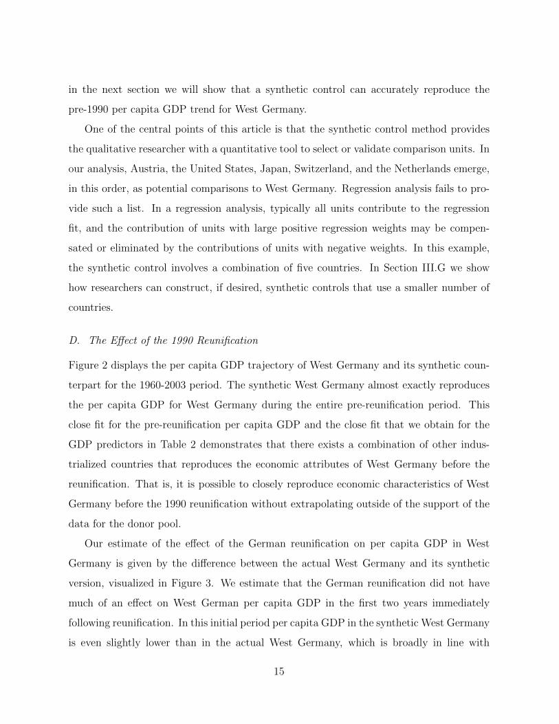
D. The Effect of the 1990 Reunification

Figure 2 displays the per capita GDP trajectory of West Germany and its synthetic coun-

terpart for the 1960-2003 period. The synthetic West Germany almost exactly reproduces

the per capita GDP for West Germany during the entire pre-reunification period. This

close fit for the pre-reunification per capita GDP and the close fit that we obtain for the

GDP predictors in Table 2 demonstrates that there exists a combination of other indus-

trialized countries that reproduces the economic attributes of West Germany before the

reunification. That is, it is possible to closely reproduce economic characteristics of West

Germany before the 1990 reunification without extrapolating outside of the support of the

data for the donor pool.

Our estimate of the effect of the German reunification on per capita GDP in West

Germany is given by the difference between the actual West Germany and its synthetic

version, visualized in Figure 3. We estimate that the German reunification did not have

much of an effect on West German per capita GDP in the first two years immediately

following reunification. In this initial period per capita GDP in the synthetic West Germany

is even slightly lower than in the actual West Germany, which is broadly in line with

15

arguments about an initial demand boom (see, for example, Meinhardt et al., 1995). From

1992 onwards, however, the two lines diverge substantially. While per capita GDP growth

decelerates in West Germany, for the synthetic West Germany per capita GDP keeps

ascending at a pace similar to that of the pre-unification period. The difference between

the two series continues to grow until the end of the sample period. Thus, our results

suggest a pronounced negative effect of the reunification on West German income. We find

that over the entire 1990-2003 period, per capita GDP was reduced by about 1600 USD per

year on average, which amounts to approximately 8 percent of the 1990 baseline level. In

2003, per capita GDP in the synthetic West Germany is estimated to be about 12 percent

higher than in the actual West Germany.

One valid concern in the context of this study is the potential existence of spillover

effects. In particular, the possibility that the German reunification had a substantial effects

in per capita GDP in countries other than Germany.19 Notice, however, that the limited

number of units in the synthetic control allows the evaluation of the existence and direction

of potential biases created by spillover effects. For example, if the German reunification had

negative spillover effects on the per capita GDP of the countries included in the synthetic

control, then the synthetic control would provide an underestimate of the counterfactual

per capita GDP trajectory for West Germany in the absence of the reunification and,

therefore an underestimate of the negative effect of the reunification on per capita GDP in

West Germany. On the other hand, if the German reunification had positive effects in the

economies included in the synthetic control this would exacerbate the negative effect of the

synthetic control estimates. Notice also that spillover effects on countries not included in

the synthetic control do not affect synthetic control estimates.

E. Placebo Studies

To evaluate the credibility of our results, we conduct a series of placebo studies where

the event of interest, that is the German reunification, is reassigned in the data set to a

19This is a violation of the Stable Unit Treatment Value Assumption (SUTVA) introduced in Rubin(1980).

16

year different than 1990 and countries different than West Germany. We first compare

the reunification effect estimated above for West Germany to a placebo effect obtained

after reassigning in our data the German reunification to a period before the reunification

actually took place. A large placebo estimate would undermine our confidence that the

results in Figure 2 are indeed indicative of the economic cost of the reunification and not

merely driven by lack of predictive power.

To conduct this placebo study we rerun the model for the case when reunification is

reassigned to the middle of the pre-treatment period in the year 1975, about 15 years earlier

than reunification actually occurred. We use the same out-of-sample validation technique

to compute the synthetic control and we lag the predictors variables accordingly for the

training and validation period. Figure 4 displays the results of this “in-time placebo”

study. The synthetic West Germany almost exactly reproduces the evolution of per capita

GDP in the actual West Germany for the 1960-1975 period. Most importantly, the per

capita GDP trajectories of West Germany and its synthetic counterpart do not diverge

considerably during the 1975-1990 period. That is, in contrast to the actual 1990 German

reunification, our 1975 placebo reunification has no perceivable effect. This suggests that

the gap estimated in Figure 2 reflects the impact of the German reunification and not a

potential lack of predictive power of the synthetic control.20

An alternative way to conduct placebo studies is to artificially reassign in the data

the event of interest, in our example the German reunification, to a comparison unit. In

this way we can obtain synthetic control estimates for countries that did not experience

the event of interest. Applying this idea to each country in the donor pool allows us

to compare the estimated effect of the German reunification on West Germany to the

distribution of placebo effects obtained for other countries. We will deem the effect of

the German reunification on West Germany significant if the estimated effect for West

Germany is unusually large relative to the distribution of placebo effects.

20We have computed similar in-time placebo studies where we reassign in our data the German reuni-fication to the years 1970 and 1980 respectively and the results are similar to the results for 1975 shownhere.

17

Figure 5 reports the ratios between the post-1990 RMSPE and the pre-1990 RMSPE for

West Germany and for all the countries in the donor pool. Recall that RMSPE measures

the magnitude of the gap in the outcome variable of interest between each country and

its synthetic counterpart. A large post-intervention RMSPE is not indicative of a large

effect of the intervention if the synthetic control does not closely reproduce the outcome

of interest prior to the intervention. That is, a large post-intervention RMSPE is not

indicative of a large effect of the intervention if the pre-intervention RMSE is also large.

For each country we divide the post-reunification RMSPE by its per-reunification RMSPE.

This metric obviates the need to discard those countries with pre-1990 per-capita GDP

values that cannot be approximated with a synthetic control. In Figure 5 West Germany

clearly stands out as the country with the highest RMSPE ratio. For West Germany the

post-reunification gap is about 16 times larger than the pre-reunification gap. If one were

to pick a country at random from the sample, the chances of obtaining a ratio as high as

this one would be 1/16 ' 0.06.

F. Robustness Test

In this section we run a robustness check to test the sensitivity of our main results to the

changes in the country weights, W ∗. Recall from Table 1 that the synthetic West Germany

is estimated as a weighted average of Austria, the United States, Japan, Switzerland, and

the Netherlands, with weights decreasing in this order. Here we iteratively re-estimate the

baseline model to construct a synthetic West Germany omitting in each iteration one of

the countries that received a positive weight in Table 1. The motivation is to check if the

estimates in section III.D are sensitive to the exclusion of any particular country from our

sample. That is, with this sensitivity check we evaluate to which extent our results are

driven by any particular country. Figure 6 displays the results. Figure 6 reproduces Figure

2 (solid and dashed black lines) incorporating the leave-one-out estimates (grey lines). This

figure shows that the results of the analysis in section III.D are fairly robust to the exclusion

of any particular country from our sample of comparison countries.

18

G. Reducing the Number of Units in a Synthetic Control

Recall that the synthetic West Germany in Figure 2 is a weighted average of five control

countries: Austria, the United States, Japan, Switzerland, and the Netherlands. Compar-

ative researchers, however, typically choose a very small number of cases, with the aim of

meticulously describing and analyzing the characteristics and outcomes of each of those

cases. As a result, in many instances, comparative researchers may favor sparse synthetic

controls; that is, synthetic controls that involve a small number of comparison countries.

Reducing the number of units in the synthetic control may, nonetheless, impact the extend

to which the synthetic control is able to fit the characteristics of the unit of interest. In

this section we examine the trade-off between sparsity and goodness of fit in the choice of

the number of units that contribute to the synthetic control for West Germany. In order

to investigate this trade-off, we construct synthetic controls for West Germanies allowing

only combinations of four, three, two, and a single control country respectively.21 Table 3

shows the countries and weights for the sparse synthetic controls. For this example, the

countries contributing to the sparse versions of the synthetic control for West Germany

are subsets of the set of five countries contributing to the synthetic control in the baseline

specification.22 Austria retains the largest weight in all instances, while the USA, Japan,

and Switzerland are second, third, and fourth in terms of their synthetic control weights.

Table 4 compares economic growth predictors of West Germany, synthetic West Ger-

many, the sparse versions of synthetic West Germany, and the OECD sample. This table

documents the sacrifice in terms of goodness of fit resulting from a reduction in the num-

ber of countries, l, allowed to contribute to the synthetic control. Overall, relative to the

baseline synthetic control with five countries, the decline in goodness of fit is moderate for

l = 4, 3, 2. The “matching” case of l = 1 produces a much worse goodness of fit relative to

l > 1, with substantial discrepancies in the per capita GDP and trade openness variables.

21More precisely, for l = 4, 3, 2, 1, and for all possible combinations of l control countries, we choose theone that produces the synthetic control unit that minimizes the loss defined in Equation (1). To reducecomputational complexity we used the weights vm obtained for the baseline model, instead of attemptingto recalculate these weights for the many different combinations of l countries.

22This is not imposed in our analysis, as we consider all possible combinations of countries among the16 countries in the donor pool, and may not necessarily be the case for other applications.

19

However, even the matching case, with l = 1, represents a large improvement in terms

of goodness of fit relative to the comparison unit consisting of the population weighted

average of the OECD sample. Figure 7 shows the per capita GDP path for West Germany

and the sparse synthetic controls with l = 4, 3, 2, 1. With the exception of the matching

case (l = 1), the sparse synthetic controls in Figure 7 produce results that are very similar

to the baseline result in Figure 2. However, using a single country as a comparison provides

a much poorer fit to the pre-1990 per capita GDP path for West Germany. This illustrates

the potential gains from using combinations of countries rather than single countries as

comparison cases in comparative research.

IV. Conclusion

There is a widespread consensus among political methodologists about the necessity to

integrate and exploit complementarities between qualitative and quantitative tools for em-

pirical research in political science. However, some of the efforts in this direction have been

denounced by qualitative methodologists as attempts to impose quantitative templates on

qualitative research that disregard or do not make use of the many genuine advantages of

qualitative research (Brady and Collier, 2004; George and Bennett, 2005). The synthetic

control method discussed in this article ‘falls in between’ the qualitative and quantitative

methodologies and provides a potentially useful tool for researchers of both traditions. On

the one hand, the synthetic control method provides a systematic way to select compari-

son units in quantitative comparative case studies. In this way, like in Card and Krueger

(1994) and Rosenbaum (2005), the synthetic control method brings to quantitative studies

the careful selection of cases that is done in qualitative analysis. In addition, by explicitly

specifying the set of units that are used for comparison, the method does not preclude but

facilitates detailed qualitative analysis and comparison between the case of interest and

the set of comparison units selected by the method. That is, the synthetic control method

can be used to guide the selection of comparison units in qualitative studies, allowing what

Tarrow (1995) calls “qualitative inference with quantitative bones”.

20

References

Abadie, A., A. Diamond, and J. Hainmueller. 2010. “Synthetic Control Methods for Compara-tive Case Studies: Estimating the Effect of California’s Tobacco Control Program.” Journalof the American Statistical Association. 105(490): 493-505.

Abadie, A. and J. Gardeazabal. 2003. “The Economic Costs of Conflict: A Case Study of theBasque Country.” American Economic Review. 93(1): 112-132.

Adams, G., L. Alexander, and J. Gagon. 1993. “German unification and the European monetarysystem: A quantitative analysis.” Journal of Policy Modeling. 15(4): 353-392.

Alesina, A., and E. Spolaore, 2003. The Size of Nations. Cambridge, MA: MIT Press.

Akerlof, G., A. K. Rose, J. L. Yellen, and H. Hessenius. 1991. “East Germany in from the Cold:The Economic Aftermath of Currency Union.” Brookings Papers on Economic Activity. 1:1-105.

Barro, R.J. and J. Lee. 1994. “Data Set for a Panel of 138 Countries.” Available at:http://www.nber.org/pub/barro.lee/.

Barro, R.J. and J. Lee. 2000. “International Data on Educational Attainment: Updates andImplications.” CID Working Paper No. 42, April 2000 – Human Capital Updated Files.

Beck, N. 2010. “Causal Process Observation: Oxymoron or (Fine) Old Wine.” Political Analysis.18(4): 499-505.

Bennett, A. and C. Elman. 2006. “Qualitative Research: Recent Developments in Case StudyMethods.” Annual Review of Political Science. 9: 455-76.

Brady, H.E. and D. Collier, Eds. 2004. Rethinking Social Inquiry: Diverse Tools, Shared Stan-dards. Lanham, MD: Rowman & Littlefield.

Card, D. and A.B. Krueger. 1994. “Minimum Wages and Employment: A Case Study of theFast-Food Industry in New Jersey and Pennsylvania.” American Economic Review. 84(4):772-93.

Collier D. 1993. “The comparative method.” In A. Finifter. Political Science: The State of theDiscipline II. Washington, DC: American Political Science Association: 105-19.

Collier D and J. Mahoney. 1996. “Insights and pitfalls: selection bias in qualitative research.”World Politics. 49(1): 56-91.

Collier D, J. Mahoney, and J. Seawright. 2004. Claiming too much: warnings about selectionbias. In Brady, H.E. and D. Collier. Rethinking Social Inquiry: Diverse Tools, SharedStandards, Eds. Lanham, MD: Rowman & Littlefield: 85-102.

Dornbusch, R. and H. Wolf. 1992. “Economic Transition in Eastern Germany.” BrookingsPapers on Economic Activity. 1: 235-261.

21

Eichengreen, B. and J.A. Frieden. 2000. The Political Economy of European Monetary Unifica-tion. Westview Press.

Fearon, J.D. 1991. “Counterfactuals and Hypothesis Testing in Political Science.” World Poli-tics. 43(2): 169-195.

Feldstein, M. 1997. “The Political Economy of the European Economic and Monetary Union:Political Sources of an Economic Liability.” Journal of Economic Perspectives. 11(4):23-42.

Geddes B. 2003. Paradigms and Sand Castles: Theory Building and Research Design in Com-parative Politics. Ann Arbor: Univ. Mich. Press.

George, A.L. and A. Bennett. 2005. Case Studies and Theory Development in the Social Sci-ences. Cambridge, MA: MIT Press.

Gerring, J. 2004. “What Is a Case Study and What Is It Good for?” American Political ScienceReview 98(2): 341-354.

Gerring, J. 2007. Case Study Research: Principles and Practices. Cambridge, MA: CambridgeUniversity Press.

Haas, E.B. 1958. The uniting of Europe: political, social, and economic forces. Stanford Uni-versity Press.

Hall, Peter. 2003. “Aligning Ontology and Methodology in Comparative Politics.” In Ma-honey, J. and D. Rueschemeyer. Comparative Historical Analysis in the Social Sciences.Cambridge, UK: Cambridge University Press: 373-429.

Hallett, A. J. and Y. Ma. 1993. “East Germany, West Germany, and Their MezzogiornoProblem: A Parable for European Economic Integration.” Economic Journal. 103(417):416-428.

Heckman, J.J. and V.J. Hotz. 1989. “Choosing Among Alternative Nonexperimental Methodsfor Estimating the Impact of Social Programs: The Case of Manpower Training.” Journalof the American Statistical Association. 84(408): 862-874.

King, G., R.O. Keohane, and S. Verba. 1994. Designing Social Inquiry: Scientific Inference inQualitative Research. Princeton, NJ: Princeton University Press.

King, G., and L. Zeng. 2006 “The Dangers of Extreme Counterfactuals.” Political Analysis.14(2): 131-159.

Lieberman, E. 2005. “Nested Analysis as a Mixed-Method Strategy for Comparative Research.”American Political Science Review. 99(3): 435-52.

Lijphart, A. 1971. “Comparative Politics and the Comparative Method.” American PoliticalScience Review. 65(3): 682-693.

Lijphart, A. 1975. “The Comparative-Cases Strategy in Comparative Research.” ComparativePolitical Studies. 8(2): 158-177.

22

Lipschitz, L., and D. McDonald. 1990. “German Unification: Economic Issues.” InternationalMonetary Fund Occasional Paper. No 75.

Mahoney, J. and D. Rueschemeyer. 2003. Comparative Historical Analysis in the Social Sciences.Cambridge, UK: Cambridge University Press.

Meinhardt, V., B. Seidel, F. Stile, and D. Teichmann. 1995. “Transferleistungen in die neuenBundeslander und deren wirtschaftliche Konsequenzen.” Deutsches Institut fur Wirtschaft-froschung, Sonderheft 154.

Mueller, G. 2000. Nutzen und Kosten der Wiedervereinigung. Baden-Baden: Nomos.

Pierson, P. and T. Skocpol. 2002. “Historical Institutionalism in Contemporary Political Sci-ence.” In Katznelson, I. and H. Millner. Political Science: The State of the Discipline.New York: W.W. Norton.

Przeworski, A., M. Alvarez, J. Cheibub, and F. Limongi. 2000. Democracy and Development:Political Institutions and Well-Being in the World, 1950-1990. Cambridge, UK: CambridgeUniversity Press.

Przeworski, A. and H. Teune. 1970. The Logic of Comparative Social Inquiry. New York, NY:Wiley.

Ragin, C.C. 1987. The Comparative Method: Moving Beyond Qualitative and QuantitativeStrategies. Berkeley, CA: University of California Press.

Rosenbaum, P.R. 2005. “Heterogeneity and Causality: Unit Heterogeneity and Design Sensitiv-ity in Observational Studies.” The American Statistician. 59(2): 147-152.

Rubin, D.B. 1980. Comment on: “Randomization analysis of experimental data in the Fisherrandomization test” by D. Basu. Journal of the American Statistical Association. 75:591-593.

Rubin, D.B. 1990. “Formal Modes of Statistical Inference for Causal Effects.” Journal ofStatistical Planning and Inference. 25: 279-292.

Siebert, H. 1992. Das Wagnis der Einheit: Eine Wirtschaftspolitische Therapie. Stuttgart:Deutsche Verlags-Anstalt.

Sekhon, J.S. 2004. “Quality Meets Quantity: Case Studies, Conditional Probability, and Coun-terfactuals.” Perspectives on Politics. 2(2): 281-293.

Tarrow, S. 1995. “Bridging the Quantitative-Qualitative Divide in Political Science.” AmericanPolitical Science Review. 89(2): 471-474.

Tarrow, S. 2010. “The Strategy of Paired Comparison: Toward a Theory of Practice.” Compar-ative Political Studies. 43(2): 230-259.

23

Data Appendix

The data sources employed for the application are:

• GDP per capita (PPP 2002 USD). Source: OECD National Accounts (retrieved via theOECD Health Database). Data for West Germany was obtained from Statistisches Bun-desamt 2005 (Arbeitskreis “Volkswirtschaftliche Gesamtrechnungen der Lander”) and con-verted using PPP monetary conversion factors (retrieved from the OECD Health Database).

• Investment Rate: Ratio of real domestic investment (private plus public) to real GDP. Thedata is reported in five year averages. Source: Barro and Lee (1994).

• Schooling: Percentage of secondary school attained in the total population aged 25 andolder. The data is reported in five year increments. Source: Barro and Lee (2000).

• Industry: industry share of value added. Source: World Bank WDI Database 2005 andStatistisches Bundesamt 2005.

• Inflation: annual percentage change in consumer prices (base year 1995). Source: WorldDevelopment Indicators Database 2005 and Statistisches Bundesamt 2005.

• Trade Openness: Export plus Imports as percentage of GDP. Source: World Bank: WorldDevelopment Indicators CD-ROM 2000.

24

Figures

Figure 1: Trends in Per-Capita GDP: West Germany vs. Rest of OECD Sample

1960 1970 1980 1990 2000

050

0010

000

1500

020

000

2500

030

000

year

per−

capi

ta G

DP

(P

PP,

200

2 U

SD

)

West Germanyrest of the OECD sample

reunification

25

Figure 2: Trends in Per-Capita GDP: West Germany vs. Synthetic West Germany

1960 1970 1980 1990 2000

050

0010

000

1500

020

000

2500

030

000

year

per−

capi

ta G

DP

(P

PP,

200

2 U

SD

)

West Germanysynthetic West Germany

reunification

26

Figure 3: Per-Capita GDP Gap Between West Germany and Synthetic West Germany

1960 1970 1980 1990 2000

−40

00−

2000

020

0040

00

year

gap

in p

er−

capi

ta G

DP

(P

PP,

200

2 U

SD

)

reunification

27

Figure 4: Placebo Reunification 1975 - Trends in Per-Capita GDP: West Germany vs.Synthetic West Germany

1960 1965 1970 1975 1980 1985 1990

050

0010

000

1500

020

000

2500

030

000

year

per−

capi

ta G

DP

(P

PP,

200

2 U

SD

)

West Germanysynthetic West Germany

placebo reunification

28

Figure 5: Ratio of post-reunification RMSPE to pre-reunification RMSPE: West Germanyand control countries.

Portugal

Austria

Denmark

France

Japan

Switzerland

UK

Belgium

Spain

New Zealand

USA

Netherlands

Greece

Norway

Australia

Italy

West Germany

●

●

●

●

●

●

●

●

●

●

●

●

●

●

●

●

●

5 10 15

Post−Period RMSE / Pre−Period RMSE

29

Figure 6: Leave-one-out distribution of the synthetic control for West Germany

1960 1970 1980 1990 2000

050

0010

000

1500

020

000

2500

030

000

year

per−

capi

ta G

DP

(P

PP,

200

2 U

SD

)

reunification

West Germanysynthetic West Germanysynthetic West Germany (leave−one−out)

30

Figure 7: Per-Capita GDP Gaps Between West Germany and Sparse Synthetic Controls

1960 1970 1980 1990 2000

050

0010

000

1500

020

000

2500

030

000

No. of control countries: 4

year

per−

capi

ta G

DP

(P

PP,

200

2 U

SD

)

West Germanysynthetic West Germany

reunification

1960 1970 1980 1990 2000

050

0010

000

1500

020

000

2500

030

000

No. of control countries: 3

yearpe

r−ca

pita

GD

P (

PP

P, 2

002

US

D)

West Germanysynthetic West Germany

reunification

1960 1970 1980 1990 2000

050

0010

000

1500

020

000

2500

030

000

No. of control countries: 2

year

per−

capi

ta G

DP

(P

PP,

200

2 U

SD

)

West Germanysynthetic West Germany

reunification

1960 1970 1980 1990 2000

050

0010

000

1500

020

000

2500

030

000

No. of control countries: 1

year

per−

capi

ta G

DP

(P

PP,

200

2 U

SD

)

West Germanysynthetic West Germany

reunification

31

Tables

Table 1: Synthetic and Regression Weights for West Germany

Synthetic Regression Synthetic RegressionCountry Control Weight Weight Country Control Weight WeightAustralia 0 0.12 Netherlands 0.10 0.14Austria 0.42 0.26 New Zealand 0 0.12Belgium 0 0 Norway 0 0.04Denmark 0 0.08 Portugal 0 -0.08France 0 0.04 Spain 0 -0.01Greece 0 -0.09 Switzerland 0.11 0.05Italy 0 -0.05 UK 0 0.06Japan 0.16 0.19 USA 0.22 0.13

Note: The synthetic weight is the country weight assigned by the synthetic control method.The regression weight is the weight assigned by linear regression. See Section II for details.

Table 2: Economic Growth Predictor Means before the German Reunification

West Synthetic OECDGermany West Germany Sample

GDP per-capita 15808.9 15800.9 8021.1Trade openness 56.8 56.9 31.9Inflation rate 2.6 3.5 7.4Industry share 34.5 34.4 34.2Schooling 55.5 55.2 44.1Investment rate 27.0 27.0 25.9

Note: GDP per capita, inflation rate, and trade openness areaveraged for the 1981–1990 period. Industry share is aver-aged for the 1981–1990 period. Investment rate and school-ing are averaged for the 1980–1985 period. The last columnreports a population weighted average for the 16 OECD coun-tries in the donor pool.

32

Table 3: Synthetic Weights from Combinations of Control Countries

Synthetic Combination: Countries and W-WeightsFive Control Countries Austria USA Japan Switzerland Netherlands

0.42 0.22 0.16 0.11 0.10Four Control Countries Austria USA Japan Switzerland

0.56 0.22 0.13 0.10Three Control Countries Austria USA Japan

0.59 0.26 0.15Two Control Countries Austria USA

0.76 0.24One Control Country Austria

1

Note: Countries and W-Weights for synthetic control constructed from best fittingcombination of five, four, three, two, and one countries. See text for details.

Table 4: Economic Growth Predictor Means before the German Reunification for Combi-nations of Control Countries

West Synthetic West Germany OECDGermany Number of countries in synthetic unit: Sample

5 4 3 2 1GDP per-capita 15808.9 15800.9 15800.5 15486.4 15576.1 14817.0 8021.1Trade openness 56.8 56.9 55.9 52.5 61.5 74.6 31.9Inflation rate 2.6 3.5 3.6 3.6 3.8 3.5 7.4Industry share 34.5 34.4 34.6 34.8 34.3 35.5 34.2Schooling 55.5 55.2 57.6 57.7 60.7 60.9 44.1Investment rate 27.0 27.0 27.2 26.8 25.6 26.6 25.9

Note: GDP per capita, inflation rate, and trade openness are averaged for the 1981–1990period. Industry share is averaged for the 1981–1990 period. Investment rate and schoolingare averaged for the 1980–1985 period.

33