Embed Size (px)
DESCRIPTION
Comparative evaluation of power plant
Citation preview

Comparative Evaluation of Power Plants with CO2 Capture:
Thermodynamic, Economic and Environmental Performance
Dissertation
Dipl.‐Ing. Fontina Petrakopoulou
Berlin

Comparative Evaluation of Power Plants
with CO2 Capture: Thermodynamic,
Economic and Environmental Performance
vorgelegt von
Diplom‐Ingenieurin
Fontina Petrakopoulou aus Griechenland
von der Fakultät III – Prozesswissenschaften
der Technischen Universität Berlin
zur Erlangung des akademischen Grades
Doktor der Ingenieurwissenschaften
– Dr.‐Ing. –
genehmigte Dissertation
Promotionsausschuss
Vorsitzender: Prof. Dr.‐Ing. Felix Ziegler
Berichter: Prof. Dr.‐Ing. Georgios Tsatsaronis
Berichter: Prof. Dr.‐Ing. Günter Wozny
Tag der wissenschaftlichen Aussprache: 6.12.2010
Berlin, 2011
D 83


Foreword
This work has been conducted during my stay as a research assistant at the Institute for
Energy Engineering and Protection of the Environmental of the Technische Universität Berlin.
During the period of September 2006 – September 2009, this research was supported by the
European Commission’s Marie Curie 6th Framework Programme of the CT‐2005‐019296‐
INSPIRE training network.
With this opportunity, I would like to express my gratitude to the people that facilitated the
completion of this work.
I am most especially grateful to Professor George Tsatsaronis, who supervised this work and
was always willing, helpful, creative and patient. His support was the most important
motivator to complete this work.
Professor Tatiana Morosuk was always present and willing to assist. Her energy and
excitement brightened some cloudy days!
I would like to thank Professor Günter Wozny for the review of this thesis. I am also thankful
to Professor Felix Ziegler for his willingness to chair my thesis defence.
I am indebted to the students that contributed to this work: Anna Carrasai, Christopher
Paitazoglou, Costanza Piancastelli, Foteini Kokkali, Ivan Gallio and Marlene Cabrera.
Special thanks to my colleagues from the INSPIRE network and the Institute for Energy
Engineering and Protection of the Environmental for the fruitful collaboration, eventful
meetings and nice experiences gathered. My close and fulfilling collaboration with Dr. Alicia
Boyano Larriba deserves a special reference.
For the comfort of a personal licence for the software EbsilonProfessional by Evonik Energy
Services GmbH, I am very grateful.
I truly appreciate the help from my companion, Alex Robinson. Without his presence and
support, the completion of this work would have been more difficult and definitely not as
fun!
Finally, I would like to thank my family for their understanding and eternal encouragement.
Berlin, October 2010
Fontina Petrakopoulou

In memory of Matteo Milanesi

Synopsis
CCS (Carbon Capture and Sequestration) in the energy sector is seen as a bridge technology for
CO2 mitigation, due to the ever‐growing environmental impact of anthropogenic‐emitted
greenhouse gases. In this work, eight power plant concepts using CO2 capture technologies
are assessed based on their efficiency, economic feasibility and environmental footprint.
Exergy‐based analyses are used for evaluating the considered power plants through
comparison with a reference plant without CO2 capture. While conventional exergy‐based
analyses provide important information that can lead to improvements in plant performance,
additional insight about individual components and the interactions among equipment can
aid further assessment. This led to the development of advanced exergy‐based analyses, in
which the exergy destruction, as well as the associated costs and environmental impacts are
split into avoidable/unavoidable and endogenous/exogenous parts. Based on the avoidable
parts, the potential for improvement is revealed, while based on the endogenous/exogenous
parts, the component interactions are obtained.
Among the examined plants with CO2 capture, the most efficient are those working with
oxy‐fuel technology. An exergoeconomic analysis shows a minimum increase in the relative
investment cost (in €/kW) of 80% for the conventional approach (chemical absorption) and an
increase of 86% for the oxy‐fuel plant with chemical looping combustion. The latter shows a
somewhat decreased environmental impact when compared to that of the reference plant. On
the contrary, the plant with chemical absorption results in a higher environmental penalty
due to its high efficiency penalty. Therefore, accepting that all assumptions and data related
to the calculations of the environmental impacts are reliable, efficiency improvement seems to
be a more significant factor in potentially decreasing a plant’s environmental impact. With
advanced exergy‐based analyses, interdependencies among components are identified, and
the real potential for cost‐ and environmental‐related improvement is revealed. A common
trend for all plants examined is that most thermodynamic inefficiencies are caused by the
internal operation of the components. Additionally, avoidable quantities are generally found
to be low for components with high costs and environmental impacts, leaving a relatively
narrow window of improvement potential.

Synopsis
iv

Table of Contents
1. Introduction....................................................................................................................................1
2. CO2 capture from power plants ..................................................................................................5
2.1 Carbon capture and storage (CCS)...................................................................................5
2.1.1 CO2 capture ...........................................................................................................5
2.1.2 CO2 transport ........................................................................................................7
2.1.3 CO2 storage............................................................................................................7
2.2 State of the art of CCS.........................................................................................................8
2.3 The plants considered in this study ...............................................................................12
2.3.1 The reference plant.............................................................................................15
2.3.2 The plant with chemical absorption using monoethanolamine (MEA
plant) ....................................................................................................................16
2.3.3 The simple oxy‐fuel concept .............................................................................18
2.3.4 The S‐Graz cycle .................................................................................................19
2.3.5 The advanced zero emission plant with 100% CO2 capture (AZEP 100) ....20
2.3.6 The advanced zero emission plant with 85% CO2 capture (AZEP 85) ........21
2.3.7 The plant with chemical looping combustion (CLC plant) ..........................22
2.3.8 The plant using a methane steam reforming membrane with
hydrogen separation (MSR plant) ....................................................................24
2.3.9 The plant using an autothermal reformer (ATR plant) .................................26
2.4 Simulation software..........................................................................................................27
2.5 Preliminary comparison...................................................................................................27
2.5.1 Simulation results ...............................................................................................27
2.5.2 Additional considerations .................................................................................28
3. Methodology – exergy‐based analyses....................................................................................31
3.1 State of the art ....................................................................................................................31
3.2 Conventional exergy‐based analyses..............................................................................33
3.2.1 Exergetic analysis ................................................................................................33
3.2.2 Exergy and economics ........................................................................................35
Table of Contents
vi
3.2.2.1 Economic analysis............................................................................. 35
3.2.2.2 Exergoeconomic analysis................................................................. 36
3.2.3 Exergy and environmental impacts ................................................................. 38
3.2.3.1 Life cycle assessment........................................................................ 38
3.2.3.2 Exergoenvironmental analysis........................................................ 39
3.3 Advanced exergy‐based analyses ...................................................................................... 41
3.3.1 Advanced exergetic analysis............................................................................. 42
3.3.1.1 Splitting the rate of exergy destruction ......................................... 42
3.3.1.2 Splitting the avoidable and unavoidable rates of exergy
destruction into endogenous and exogenous parts ..................... 43
3.3.1.3 Calculating the total avoidable exergy destruction ..................... 43
3.3.2 Advanced exergoeconomic analysis ................................................................ 44
3.3.2.1 Splitting the cost rates of investment and exergy destruction.... 45
3.3.2.2 Calculating the total rates of avoidable costs................................ 44
3.3.3 Advanced exergoenvironmental analysis....................................................... 47
3.3.3.1 Calculating the total avoidable environmental impact of
pollutant formation and exergy destruction................................. 47
4. Application of the exergy‐based analyses to the plants ...................................................... 51
4.1 Conventional exergy‐based analyses ............................................................................ 51
4.1.1 Exergetic analysis............................................................................................... 51
4.1.2 Exergy and economics....................................................................................... 54
4.1.2.1 Results of the economic analysis .................................................... 54
4.1.2.2 Results of the exergoeconomic analysis......................................... 55
4.1.2.3 Sensitivity analyses........................................................................... 58
4.1.3 Exergy and environmental impacts ................................................................ 59
4.1.3.1 Results of the life cycle assessment ................................................ 59
4.1.3.2 Results of the exergoenvironmental analysis ............................... 60
4.1.3.3 Sensitivity analyses........................................................................... 61
4.2 Advanced exergy‐based analyses .................................................................................. 70
4.2.1 Advanced exergetic analysis ............................................................................ 70
4.2.1.1 Application of the advanced exergetic analysis ........................... 70
4.2.1.2 Splitting the exergy destruction...................................................... 74
4.2.1.3 Splitting the exogenous exergy destruction.................................. 77
4.2.1.4 Calculating the total avoidable rate of exergy destruction ......... 78
4.2.2 Advanced exergoeconomic analysis ............................................................... 79

Table of Contents
vii
4.2.2.1 Splitting the investment cost rates ..................................................80
4.2.2.2 Splitting the cost rate of exergy destruction ..................................82
4.2.2.3 Splitting the exogenous cost rates of investment and exergy
destruction..........................................................................................84
4.2.2.4 Calculating the total avoidable cost rates associated with
plant components ..............................................................................87
4.2.3 Advanced exergoenvironmental analysis.......................................................88
4.2.3.1 Splitting the environmental impact of exergy destruction..........89
4.2.3.2 Splitting the environmental impact of pollutant formation........90
4.2.3.3 Splitting the exogenous environmental impact of exergy
destruction..........................................................................................90
4.2.3.4 Calculating the total avoidable environmental impact of
exergy destruction.............................................................................92
5. Conclusions .................................................................................................................................. 95
5.1. Exergetic analysis.............................................................................................................. 96
5.2. Economic analysis............................................................................................................. 97
5.3. Exergoeconomic analysis................................................................................................. 97
5.4. Life cycle assessment........................................................................................................ 97
5.5. Exergoenvironmental analysis........................................................................................ 98
5.6. Advanced exergetic analysis ........................................................................................... 98
5.7. Advanced exergoeconomic analysis .............................................................................. 98
5.8. Advanced exergoenvironmental analysis ..................................................................... 99
5.9. Summary and future work .............................................................................................. 99
Appendices
A. Flow charts and simulation assumptions of the power plants ......................................... 101
A.1. The reference plant ......................................................................................................... 102
A.2. The AZEP 85.................................................................................................................... 108
A.3. The AZEP 100.................................................................................................................. 118
A.4. The MCM reactor............................................................................................................ 124
A.5. The CLC plant ................................................................................................................. 125
A.6. The MEA plant ................................................................................................................ 135
A.7. The S‐Graz cycle.............................................................................................................. 145
A.8. The ATR plant ................................................................................................................. 149
A.9. The MSR plant................................................................................................................. 153
A.10. The simple oxy‐fuel plant .............................................................................................. 157

Table of Contents
viii
B. Assumptions used in the sumulations and the conventional analyses...........................161
B.1 Calculation of efficiencies and pressure drops for common components of the
power plants .................................................................................................................... 161
B.1.1 Compressors and expanders of GT systems (C1 and GT1) and
CO2/H2O expanders (GT2).............................................................................. 161
B.1.2 Remaining compressors.................................................................................. 161
B.1.3 Steam turbines.................................................................................................. 163
B.1.4 Pumps................................................................................................................ 163
B.1.5 Generators and motors.................................................................................... 164
B.1.6 Heat exchangers............................................................................................... 165
B.1.6.1 Pressure drops..................................................................................165
B.1.6.2 Minimum temperature differences (ΔΤmin) ..................................167
B.1.7 Reactors ............................................................................................................. 167
B.2 Application of the conventional exergy‐based methods .......................................... 168
B.2.1 Application of the exergetic analysis ............................................................ 168
B.2.2 Application of the economic analysis ........................................................... 168
B.2.3 Application of the exergoeconomic analysis................................................ 172
B.2.4 Application of the LCA................................................................................... 173
B.2.5 Application of the exergoenvironmental analysis....................................... 178
C. Design estimates for construction, operational costs and environmental impact of
heat exchangers ....................................................................................................... 179
C.1 Calculation of the surface area, A .................................................................................179
C.1.1 Calculation of the overall heat transfer coefficient.......................................179
C.1.1.1 Calculation of the non‐luminous heat transfer coefficient, Nh .180
C.1.1.2 Calculation of the convective heat transfer coefficient, ch .........183
C.1.1.3 Calculation of the tube‐side coefficient, ih ..................................185
C.1.2 Design of the tubes ...........................................................................................188
C.1.3 Materials.............................................................................................................189
D. Generalized costing equations............................................................................................... 193
References ........................................................................................................................................ 197

List of Figures
Figure 2.1: CO2 capture groups and their characteristics.................................................................5
Figure 2.2: Options for geological storage of CO2.............................................................................8
Figure 2.3: 275 CCS projects of all industrial sectors and scales, categorized by country.........10
Figure 2.4: Breakdown of the 213 active/planned projects classified by capture type...............11
Figure 2.5: Simplified diagram of the reference plant ....................................................................15
Figure 2.6: Simplified diagram of the MEA plant...........................................................................16
Figure 2.7: Simplified diagram of a CAU.........................................................................................17
Figure 2.8: Exergetic efficiency and energy requirement relative to the lean sorbent CO2
loading..............................................................................................................................18
Figure 2.9: Simplified diagram of the simple oxy‐fuel plant.........................................................18
Figure 2.10: Simplified diagram of the S‐Graz cycle.......................................................................19
Figure 2.11: Simplified diagram of the AZEP 100...........................................................................20
Figure 2.12: Structure of the MCM reactor.......................................................................................21
Figure 2.13: Simplified diagram of the AZEP 85.............................................................................22
Figure 2.14: Configuration of the CLC unit and the chemical reactions......................................24
Figure 2.15: Simplified diagram of the CLC plant ..........................................................................24
Figure 2.16: Simplified diagram of the MSR plant..........................................................................25
Figure 2.17: Configuration of the MSR reactor and the chemical reactions ................................25
Figure 2.18: Simplified diagram of the plant with an ATR............................................................26
Figure 3.1: General structure of the Eco‐indicator 99 LCIA method............................................38
Figure 3.2: Options for splitting the exergy destruction in an advanced exergetic analysis.....41
Figure 4.1: Influence of the investment cost of the MCM reactor, the CLC reactors and the
CAU on the overall COE of the respective plants ......................................................59
Figure 4.2: Influence of pollutant formation on the EIE of the reference and MEA‐0.2
plants, with consideration of an environmental impact of 4.9 Pts/t of CO2
associated with transport and storage..........................................................................62
Figure 4.3: Influence of pollutant formation (on the EIE of the reference and MEA‐0.2
plants, without consideration of the environmental impact associated with
CO2 transport and storage..............................................................................................62
Figure 4.4: The GT system of the reference plant............................................................................73
Figure 4.5: The CLC unit as part of the GT system of the CLC plant...........................................73
Figure 4.6: The MCM reactor as part of the GT system of the AZEP 85 ......................................74
List of Figures
x
Figure A.1.1: Structure of the reference plant ............................................................................... 102
Figure A.2.1: Structure of the AZEP 85.......................................................................................... 108
Figure A.3.1: Structure of the AZEP 100........................................................................................ 118
Figure A.4.1: The MCM reactor ...................................................................................................... 124
Figure A.5.1: Structure of the CLC plant ....................................................................................... 125
Figure A.6.1: Structure of the MEA plant...................................................................................... 135
Figure A.7.1: Structure of the S‐Graz cycle.................................................................................... 145
Figure A.8.1: Structure of the ATR plant ....................................................................................... 149
Figure A.9.1: Structure of the MSR plant....................................................................................... 153
Figure A.10.1: The simple oxy‐fuel plant ...................................................................................... 157
Figure B.1: Influence of mass flow on the pump efficiency ........................................................ 163
Figure B.2: Influence of the capacity on the pump efficiency..................................................... 165
Figure B.3: Connection between condenser and cooling tower ................................................. 173
Figure C.1: Graphs used for the estimation of the hN and for beam length evaluation............181
Figure C.2: Estimation of gas emissivity at different flue gas temperatures and beam
lengths............................................................................................................................ 182
Figure C.3: Estimation of the factor K at different wall and flue gas temperatures .................182
Figure C.4: Estimation of the hN at different temperatures and beam lengths ..........................182
Figure C.5: Estimation of the hc of different gases at different temperatures............................185
Figure C.6: Influence of the ho and hi variation on the Uo.............................................................185
Figure C.7: Effect of fin geometry on performance.......................................................................189

List of Tables
Table 2.1: Storage options.....................................................................................................................7
Table 2.2: Operating CCS projects in the power generation industry............................................9
Table 2.3: Operating commercial‐scale, integrated CCS projects ...................................................9
Table 2.4: Completed CCS projects of all industrial sectors ..........................................................11
Table 2.5: Main operating parameters ..............................................................................................13
Table 2.6: Efficiency, generated power, and internal power consumption for the
considered plant ................................................................................................................28
Table 3.1: Splitting the costs ............................................................................................................... 46
Table 3.2: Splitting the environmental impacts ............................................................................... 49
Table 4.1: Selected results of the exergetic analysis ........................................................................ 51
Table 4.2: Selected results of the economic analysis ....................................................................... 54
Table 4.3: Selected results of the LCA............................................................................................... 60
Table 4.4: Environmental impact of overall and avoided pollutant formation due to CO2
capture................................................................................................................................. 60
Table 4.5: Results of the conventional exergy‐based analyses for the overall plants................. 63
Table 4.6: Selected results at the component level for the reference plant .................................. 63
Table 4.7: Selected results at the component level for the AZEP 85 ............................................. 64
Table 4.8: Selected results at the component level for the AZEP 100 ........................................... 65
Table 4.9: Selected results at the component level for the CLC plant .......................................... 66
Table 4.10: Selected results at the component level for MEA‐0.2.................................................. 67
Table 4.11: Selected results at the component level for MEA‐0 .................................................... 68
Table 4.12: Selected results at the component level for the S‐Graz cycle and the simple oxy‐
fuel plant............................................................................................................................. 69
Table 4.13: Selected results at the component level for the MSR and ATR plants ..................... 69
Table 4.14: Assumptions related to the theoretical and unavoidable operation of the
components ........................................................................................................................ 71
Table 4.15: Selected results at the component level of the advanced exergetic analysis ........... 76
Table 4.16: Splitting the exogenous rate of exergy destruction..................................................... 77
Table 4.17: Splitting the rate of exergy destruction caused by each component ........................ 79
Table 4.18: Assumptions for the calculation of the unavoidable investment cost rates ............ 80
Table 4.19: Splitting the investment cost rates................................................................................. 81

List of Tables
xii
Table 4.20: Selected results from splitting the exergy destruction cost rates...............................83
Table 4.21: Selected results from splitting the exogenous investment cost rate..........................85
Table 4.22: Selected results from splitting the exogenous cost rates of exergy destruction ......86
Table 4.23: Avoidable investment cost rate......................................................................................87
Table 4.24: Avoidable exergy destruction cost rate.........................................................................87
Table 4.25: Ranking of the components with the highest total avoidable cost rate ....................88
Table 4.26: Selected results from splitting the environmental impact of exergy destruction ...89
Table 4.27: Splitting the environmental impact of pollutant formation.......................................90
Table 4.28: Selected results from splitting the exogenous environmental impact of exergy
destruction ..........................................................................................................................91
Table 4.29: Avoidable environmental impact of exergy destruction............................................92
Table 5.1: The four most influential components as ranked by each analysis.............................95
Table A.1.1: Results of the year‐by‐year economic analysis for the reference plant................ 103
Table A.1.2: Results at the component level for the reference plant.......................................... 104
Table A.1.3: Results at the stream level for the reference plant.................................................. 105
Table A.1.4: Splitting the exergy destruction in the reference plant.......................................... 106
Table A.1.5: Splitting the investment cost rate in the reference plant ....................................... 106
Table A.1.6: Splitting the cost rate of exergy destruction in the reference plant...................... 107
Table A.1.7: Splitting the environmental impact of exergy destruction in the reference
plant .................................................................................................................................. 107
Table A.2.1: Results of the economic analysis for the AZEP 85.................................................. 109
Table A.2.2: Results at the component level for the AZEP 85..................................................... 110
Table A.2.3: Results at the stream level for the AZEP 85 ............................................................ 112
Table A.2.4: Splitting the exergy destruction in the AZEP 85..................................................... 114
Table A.2.5: Splitting the investment cost rate in the AZEP 85 .................................................. 115
Table A.2.6: Splitting the cost rate of exergy destruction in the AZEP 85 ................................ 116
Table A.2. 7: Splitting the environmental impact of exergy destruction in the AZEP 85 ....... 117
Table A.3.1: Results of the economic analysis for the AZEP 100................................................ 119
Table A.3.2: Results at the component level for the AZEP 100................................................... 120
Table A.3.3: Results at the stream level for the AZEP 100 .......................................................... 122
Table A.5.1: Results of the economic analysis for the CLC plant ............................................... 126
Table A.5.2: Results at the component level for the CLC plant.................................................. 127
Table A.5.3: Results at the stream level for the CLC plant.......................................................... 129
Table A.5.4: Splitting the exergy destruction in the CLC plant.................................................. 131
Table A.5.5: Splitting the investment cost rate in the CLC plant ............................................... 132
Table A.5.6: Splitting the cost rate of exergy destruction in the CLC plant.............................. 133

List of Tables
xiii
Table A.5.7: Splitting the environmental impact of exergy destruction in the CLC plant ......134
Table A.6.1: Results at the component level for MEA‐0.2............................................................138
Table A.6.2: Results at the component level for MEA‐0...............................................................139
Table A.6.3: Results at the stream level for MEA‐0.2....................................................................140
Table A.6.4: Results at the stream level for MEA‐0.......................................................................143
Table A.7.1: Results at the component level for the S‐Graz cycle ...............................................146
Table A.7.2: Results at the stream level for the S‐Graz cycle.......................................................147
Table A.8.1: Results at the component level for the ATR plant ..................................................150
Table A.8.2: Results at the stream level for the ATR plant ..........................................................151
Table A.9.1: Results at the component level for the MSR plant ..................................................154
Table A.9.2: Results at the stream level for the MSR plant ..........................................................155
Table A.10.1: Results at the component level for the simple oxy‐fuel plant .............................158
Table A.10.2: Results at the stream level for the simple oxy‐fuel plant .....................................159
Table B.1: Efficiencies of C1, GT1 and GT2....................................................................................161
Table B.2: Efficiencies of the remaining compressors of the plants............................................162
Table B.3: Calculated efficiencies of pumps...................................................................................164
Table B.4: Pressure drops within the HXs of the reference, MEA and simple oxy‐fuel
plants .................................................................................................................................166
Table B.5: Power plant characteristics ............................................................................................168
Table B.6: Data for cost calculations................................................................................................170
Table B.7: Assumptions involved in the economic analysis........................................................172
Table B.8: Typical construction materials for process equipment ..............................................174
Table B.9: Design data for plant components ................................................................................176
Table B.10: EI of incoming and exiting streams of the systems...................................................178
Table C.1: Beam length L ..................................................................................................................181
Table C.2: Approximation of the hN with mass ratios 8:1 H2O and 25:1 CO2 ............................183
Table C.3: Gas and steam properties ..............................................................................................184
Table C.4: Estimation of the hc for high concentrations of CO2 and H2O...................................185
Table C.5: Data of the reference plant.............................................................................................186
Table C.6: Data for the AZEP 85......................................................................................................186
Table C.7: Data for the AZEP 100....................................................................................................187
Table C.8: Data of the plant with CLC............................................................................................187
Table C.9: Data for MEA‐0 ...............................................................................................................188
Table C.10: Data for MEA‐0.2 ..........................................................................................................188
Table C.11: Main construction materials of HRSGs......................................................................190
Table C.12: Design estimates for the HXs of the reference plant ................................................191

List of Tables
xiv

Nomenclature
Symbols
a Size exponent
A Surface area (m2)
b Environmental impact per unit of exergy (Pts/GJ)
B Environmental impact rate associated with exergy (Pts/h)
c Cost per unit of exergy (€/GJ)
C Cost rate associated with an exergy stream (€/h)
,i od d Inside and outside tube diameter (in)
E Exergy rate (MW)
f Exergoeconomic factor (%)
bf Exergoenvironmental factor (%)
G Total inlet flue gas flow rate (kmol/h); gas mass velocity (lb/ft2h)
,i oh h Tube‐side and gas‐side coefficients (W/m2K)
,c Nh h Convective and non‐luminous heat transfer coefficients(W/m2K)
K Constant
L Total sorbent flow rate (kmol/h); beam length (m)
m Mass flow rate (kg/s)
mwlean Average molecular weight of the lean sorbent (kg/kmol)
p Pressure (bar)
r Relative cost difference (%)
br Relative environmental impact difference (%)
,T LS S Longitudinal and transverse pitch (in)
T Temperature (°C)
oU Overall heat transfer coefficient (W/m2K)
V Volumetric flow rate (m3/s)
y Exergy destruction ratio (%)
Y Component‐related environmental impact (Pts/h)
2COy CO2 concentration (w/w, %)
Z Cost rate associated with capital investment (€/h)
Subscripts
CH Chemical (exergy)

Nomenclature
xvi
D Destruction (exergy)
F Fuel (exergy)
i, j Entering and exiting exergy stream indices
in Incoming
is Isentropic (efficiency)
, , ,k r Y W Component indices
L Loss (exergy)
l, m, n Counting indices
out Outgoing
P Product (exergy)
PH Physical (exergy)
pol Polytropic (efficiency)
tot Overall system
mech Mechanical (efficiency)
Superscripts
AV Avoidable
UN Unavoidable
UN,EN Unavoidable endogenous
UN,EX Unavoidable exogenous
AV,EN Avoidable endogenous
AV,EX Avoidable exogenous
MX Mexogenous
PF Pollutant formation
Abbreviations
AR Air reactor
ASU Air separation unit
ATR Autothermal reformer
AZEP Advanced zero emission plant
CAU Chemical absorption unit
CC Combustion chamber
CCS Carbon capture and storage
CEPCI Chemical engineering plant cost index
CLC Chemical looping combustion
COA‐CO2 Cost of avoided CO2
COE Cost of electricity
COND Condenser
COOL Cooler
CPO Catalytic partial oxidation
CT Cooling tower
Nomenclature
xvii
DB Duct burner
EC Economizer
ECBMR Enhanced coal bed methane recovery
EGR Enhanced gas recovery
EIE Environmental impact of electricity
EOR Enhanced oil recovery
EV Evaporator
FC Fuel cost
FCI Fixed capital investment
FG Flue gas
FR Fuel reactor
GEN Generator
GT Gas turbine
HP / IP / LP High pressure / intermediate pressure / low pressure
HT / LP High temperature / low temperature
HTT High‐temperature turbine
HRSG Heat‐recovery steam generator
HX Heat exchanger
IC Investment cost
ID Inside diameter
IGCC Integrated gasification combined cycle
LCA Life cycle assessment
LCIA Life cycle impact assessment
LHV Lower heating value
LNG Liquefied natural gas
LPG Liquefied petroleum gases
LPT Low‐pressure gas turbine
MEA Monoethanolamine
MCM Mixed conducting membrane
MMV Measurement, monitoring and verification
MSR Hydrogen separating membrane
NG Natural gas
NG PH Natural gas preheater
O&M Operating and maintenance costs
OC Oxygen carrier
OD Outside diameter
PEC Purchased equipment Cost
RH Reheater
SH Superheater
ST Steam turbine
TCI Total capital investment
TRR Total revenue requirement

Nomenclature
xviii
Greek symbols
Exergetic efficiency (%)
g Gas emissivity
Energetic efficiency (%)
Excess air fraction
Density (lb/ft3)
Annual operating hours
lean Lean sorbent CO2 loading

1. Introduction
Greenhouse gases absorb and trap heat in the lower atmosphere. A continuous, rapid increase in
anthropogenic atmospheric greenhouse gas concentrations since the industrial revolution has led
to pronounced temperature increases and climate change. Accounting for about 80% of the
enhanced global warming effect, CO2 is thought to be the main contributor among the
greenhouse gases (VGB PowerTech, 2004). Electric‐power generation remains the single largest
source of CO2 emissions, equal to those of the rest of the industrial sectors combined (IPCC,
2005). Additionally, most of the energy demand across the globe is covered by fossil fuels that
generate large amounts of pollutants like CO2, CH4 and NOX. An ever‐increasing demand for
energy prolongs environmental aggravation, but it simultaneously acts as a strong motivator for
the development of new technologies to mitigate climate change. As mentioned in the IPCC
report (2005), measures to reduce the increasing man‐made CO2 concentration in the atmosphere
include: (1) reducing energy demand; (2) increasing the efficiency of energy conversion and/or
fuel utilization; (3) switching to less carbon intensive fuels; (4) increasing the use of renewable
energy sources or nuclear energy; (5) sequestering CO2 by enhancing biological absorption
capacity in forests and soils and (6) carbon capturing and storing (CCS).
Carbon capture and storage is a three step process: (1) CO2 capture and compression to a
high pressure, (2) CO2 transport to a selected storage site and (3) CO2 storage. CCS from power
plants is a topic that started attracting attention from a large group of scientists only a little more
than three decades ago, as a powerful tool for limiting the impact of fossil‐fuel use on the climate
(Herzog, 2001). This field is, therefore, still in its infancy, but expertise is growing.
When evaluating options for CO2 capture from power stations, engineers are faced with a
large variety of alternative approaches. However, dissimilar assumptions and hypotheses in
evaluations make the comparison and assessment of different concepts difficult, if not infeasible.
Moreover, although several alternative approaches for capturing CO2 have been proposed in
such a short time, few appear promising with respect to efficiency and cost, while the
environmental impact of the technologies is still unknown. Although energy‐based comparative
studies of selected CO2 capture technologies have been sporadically performed in the last decade
(e.g., Kvamsdal et al., 2007; Bolland, 1991; Bolland and Mathieu, 1998), a complete presentation
and comparison of a fair number of alternative methods is still missing. Any emission reduction
(up to practically 100%) can be achieved with a sufficiently high level of expenditure. The
question, however, is whether a CO2 capture technology is a reasonable measure when balancing
the benefit to the environment against a greatly increased cost and risk (VGB PowerTech, 2004).
Chapter 1. Introduction
2
This thesis aims to evaluate a variety of CO2 capture technologies, taking into account both
the economic and the environmental perspectives (risk assessment is not included). Eight low‐ or
zero‐emission power plants with different CO2 capture technologies are presented and compared
under equivalent conditions, based on their efficiency, economic feasibility and environmental
footprint. The focus is the evaluation of CO2 capture technologies integrated in combined cycle
power plants operating with natural gas and used for electricity production. Advantages and
disadvantages of each technology and ways to reduce the cost and environmental impact
associated with electricity production, while keeping the CO2 emissions at a minimum level, are
discussed.
The methods used for the evaluation of the plants are based on exergy principles. An
exergetic analysis is the first step in evaluating an energy conversion system, identifying the source
and cause of incurred thermodynamic inefficiencies (Bejan et al., 1996; Tsatsaronis and Cziesla,
2002; Moran and Shapiro, 2008; Tsatsaronis and Cziesla, 2009). The combination of an exergetic
analysis with an economic analysis and a life cycle assessment constitutes the exergoeconomic analysis
(Bejan et al. 1996; Tsatsaronis and Cziesla 2002; Lazzaretto and Tsatsaronis, 2006) and the
exergoenvironmental analysis (Meyer et al., 2009; Tsatsaronis and Morosuk, 2008a and 2008b),
respectively.
With conventional exergy‐based analyses, information about improvements of an energy
conversion system is revealed. Monetary costs and environmental impacts are assigned to all
exergy streams of the plants, as well as to the exergy destruction incurred within each plant
component, exposing appropriate compromises among thermodynamic, economic and
environmental considerations. However, although conventional exergy‐based analyses uncover a
path towards plant improvement, they suffer from some limitations, which are addressed by
advanced exergy‐based analyses.
Advanced exergy‐based methods identify mutual interdependencies among plant
components, and reveal the real improvement potential both at the component and plant level
(Tsatsaronis, 1999a; Tsatsaronis and Park, 2002; Cziesla et al., 2006; Morosuk and Tsatsaronis,
2006a, 2006b, 2007a, 2007b, 2008a, 2008b, 2009a and 2009b; Tsatsaronis et al., 2006; Tsatsaronis
and Morosuk, 2007, 2010; Kelly 2008; Boyano et al., 2009; Kelly et al, 2009; Tsatsaronis et al., 2009).
Data obtained from advanced exergy‐based methods are crucial for pinpointing strengths and
weaknesses of complex plants with a large number of interrelated components.
This thesis is the first evaluation of CO2 capture technologies using exergoeconomic and
exergoenvironmental analyses, and it is the first complete and thorough application of the
advanced methods to complex energy conversion systems in general. Chapter 2 provides a short
description of the different steps involved in CCS technology, as well as an overview of the state
of the art. Global CCS projects are also presented and categorized based on their size, application
sector and state of realization (Section 2.2). A detailed description of the eight CO2 capture
technologies considered in this thesis, and their incorporation into power plants, is provided in
Section 2.3. Chapter 3 presents the exergy‐based methods used for the evaluation of the plants.
Both conventional and advanced exergy‐based methods are described, and all the required

Chapter 1. Introduction
3
mathematical equations and variables of the methodologies are included. Chapter 4 presents the
application of the exergy‐based methods to the simulated systems and the results obtained.
Lastly, conclusions and future plans are included in Chapter 5. The appendices and the
supplemental data provide additional detailed information for the analytical study of the results.

Chapter 1. Introduction
4

Chapter 2. CO2 capture from power plants
5
2. CO2 capture from power plants
2.1 Carbon capture and storage (CCS)
The three steps comprising CCS are CO2 capture, transport and storage. Transport and
storage of carbon dioxide are not the focus of this thesis. However, here, in order to present
the complete chain of the CCS process, information about all three steps is provided.
2.1.1 CO2 capture
CO2 capture methods can be classified into two main categories1, depending on whether the
CO2 is captured before or after the combustion process (Figure 2.1). However, the main
distinction among capture methods stems from the treatment of the fuel used: when no
treatment of the fuel occurs, the method is classified as post‐combustion capture, while when
the fuel undergoes a de‐carbonization process, the method is classified as pre‐combustion
capture.
Figure 2.1: CO2 capture groups and their characteristics
When air is used as the oxidant in post‐combustion capture, CO2 is captured with
chemical or physical solvents. The most conventional representative of this type of CO2
capture is chemical absorption, a process developed about 70 years ago to remove acid gases
1 In literature, CO2 capture technologies are generally separated into three groups: post-, pre- and oxy-combustion concepts. Although post- and pre-combustion refer to when the carbon capture takes place, oxy-combustion refers to the oxidant type used in the combustion process. Here the distinction is based exclusively on when the carbon capture takes place. Thus, oxy-combustion is considered part of the post-combustion methods (since the produced CO2 is separated after the combustion process).

Chapter 2. CO2 capture from power plants
6
from natural gas streams (Herzog, 2001). The advantages of post‐combustion capture are that
existing plants can be retrofitted with a capture unit without further rearrangements, and that
the technology is well established. However, the prominent disadvantage of the method is
the very significant amount of thermal energy required for the regeneration of the chemicals
used, resulting in a significant efficiency penalty. In recent years, many studies have
reviewed different post‐combustion technologies and compared the effectiveness of different
types of absorbents for chemical absorption (e.g., Rubin and Rao, 2002; Kothandaraman et al.,
2009). Analyses have yet to reveal any significant breakthrough, so chemical absorption
remains one of the most energy intensive methodologies.
When oxygen is used as the oxidant in post‐combustion capture (oxy‐fuel combustion), the
energy demand is reduced, when compared to chemical absorption, and the CO2 separation
process is simplified. Because oxygen is used, the combustion products consist mainly of
water vapour and carbon dioxide; the carbon dioxide is freed after the water is condensed
without requiring further treatment, keeping the energy demand of CO2 separation at
relatively low levels. In addition, with oxy‐fuel combustion, NOX emissions are reduced to
less than 1 ppm for natural gas use (Sundkvist et al., 2005). The most common method to
produce oxygen for large‐scale oxy‐fuel plants is a cryogenic air separation unit (ASU).
However, compression and the energy requirement of the distillation column included in the
process result in a relatively high cost that makes the method less attractive. Oxy‐fuel
concepts also have implementation challenges associated with technological limitations of the
components (Wilkinson et al., 2003; Anderson et al. 2008). Nevertheless, there has recently
been a large increase in projects associated with newly introduced oxy‐fuel approaches. These
technologies include oxygen‐separating membranes and new types of reactors that seem
promising with respect to their efficiency and their relatively low CO2 capture cost (e.g.,
(Kvamsdal et al., 2007).
In pre‐combustion methods, suitable de‐carbonization methods are applied to the
available fuel to separate the carbon contained in it before the combustion process. The goal is
to produce a hydrogen‐based fuel that will result in clean combustion gases. If the de‐
carbonization method results in a mixture of CO2 and gases that do not allow the required
purity of CO2 for separation (e.g., CO2 mixed with N2), chemical absorption is used.
Otherwise, if the produced CO2 is kept separate by the de‐carbonization process, no
additional treatment is needed and the CO2 is captured after water condensation. The de‐
carbonization of the fuel is highly energy demanding, relatively expensive and its
implementation requires large structural changes to any pre‐existing plant. One of the most
well‐known technologies that can be easily adopted for pre‐combustion capture is the
gasification of coal. From this process syngas is produced, which can be used in gas turbines,
increasing the overall efficiency of the plant. However, integrated gasification combined cycles
(IGCCs), present challenges that delay the broader acceptance of this technology.

Chapter 2. CO2 capture from power plants
7
2.1.2 CO2 transport
Once CO2 has been captured, it must be transported to a storage facility as gas, liquid or solid.
Transportation can be performed via pipeline, ship, rail, truck or a combination of these
means.
Transport of CO2 by pipeline in the liquid phase (above 7.58 MPa, ambient temperature)
is, at present, the most economical means of moving large quantities of CO2 long distances.
Transportation infrastructure would be needed for large quantities of CO2 to make a
significant contribution to climate change mitigation, and would imply a large network of
pipelines. As growth continues, it may become more difficult to secure rights‐of‐way for the
pipelines, particularly in highly populated zones that produce large amounts of carbon
dioxide. Existing experience has only been in zones with low population densities, and safety
issues will most probably become more complicated in populated areas. Although some
experience has been gained by enhanced oil recovery (EOR) operations, the standards required
for CCS are not necessarily the same and, therefore, new minimum standards for pipeline
quality for CCS are required (IPCC, 2005).
In some cases, transport of CO2 by ship may be economically more attractive,
particularly when the CO2 must be moved over large distances or overseas (IPCC, 2005). The
properties of liquefied CO2 are similar to those of liquefied petroleum gases (LPG). LPG
technology could be scaled‐up to large CO2 carriers, transporting CO2 by ship in a similar
way (typically at a pressure of 0.7 MPa).
Road and rail tankers are also technically feasible options when there is no access to
pipeline facilities or when the captured gas must be transferred over large distances. Here the
CO2 is transported at a temperature of ‐20°C and at a pressure of 2 MPa. These systems are
more expensive compared to pipelines and ships, except on a very small‐scale.
2.1.3 CO2 storage
Available alternative choices for CO2 storage are shown in Table 2.1. Carbon dioxide capture
with storage in deep geological formations is currently the most advanced and the most likely
approach to be deployed on a large scale in the future. Possible geological storage formations
include oil and gas fields, saline formations, and coal beds (see Figure 2.2).
Table 2.1: Storage options (WorleyParsons, 2009)a
Geological Ocean Beneficial reuse Terrestrial
Saline formations CO2 lakes Enhanced oil recovery (EOR) Forest lands
Depleted oil and gas reservoirs Solid hydrate Enhanced gas recovery (EGR) Agricultural lands including
biochar
Unmineable coal seams Dissolution Enhanced coal bed methane recovery
(ECBMR)
Grassland and grazing land
management
Salt caverns Algae farming for recycling Deserts and degraded lands
Basalt formations Other industrial manufacturing Wetlands or peat lands
Shale formations a CO2 can also be stored in other materials, i.e., through mineral carbonation (IPCC, 2005)

Chapter 2. CO2 capture from power plants
8
Everywhere under a thin overlay of soils or sediments, the earth’s surface is made up
primarily of two types of rocks: those formed by cooling magma and those formed as thick
accumulations of sand, clay, salts, and carbonates over millions of years. Sedimentary basins
consist of many layers of sand, silt, clay, carbonate, and evaporite (rock formations composed
of salt deposited from evaporating water). The sand layers provide storage space for oil,
water, and natural gas. The silt, clay and evaporite layers provide the seal that can trap these
fluids underground for periods of millions of years and longer (Benson and Franklin, 2008).
Sedimentary basins often contain many thousands of meters of sediments, where the
tiny pore spaces in the rocks are filled with salt water (saline formations). Oil and gas
reservoirs are found under such fine‐textured rocks and the mere presence of the oil and gas
demonstrates the presence of a suitable reservoir seal. In saline formations, where the pore
space is initially filled with water, after the CO2 has been underground for hundreds to
thousands of years, chemical reactions will dissolve some or all of the CO2 in the salt water,
and eventually some fraction of the CO2 will be converted into carbonate minerals, thus
becoming part of the rock itself.
2
2.2 State of the art of CCS
The first commercial plants with post‐combustion CO2 capture were constructed in the
late 1970s and early 1980s in the United States. These projects did not treat CO2 as a pollutant,
but as a new economic resource (Herzog, 2001), separating and injecting CO2 into oil
reservoirs to increase their productivity (EOR). This also led to the first long‐distance CO2
pipelines. However, with the decline of the oil price in the mid‐1980s, the separation of CO2
was too expensive, forcing the closure of these capture facilities. An exception is the North
2 http://www.co2crc.com.au/
Figure 2.2: Options for geological storage of CO2 (CO2CRC) 2

Chapter 2. CO2 capture from power plants
9
Table 2.2: Operating CCS projects in the power generation industry (Source: WorleyParsons, 2009)
Project name Capture type Country Feedstock Size CO2 use (current or planned)
Sua Pan Post‐combustion Botswana Coal 109,500 tpa CO2, 20MW Carbonation of brine
Loy Yang Power (LYP)/CSIRO PCC Project Post‐combustion Australia Coal 1,000 tpa CO2 Vent
Munmorah PCC Pilot Plant Project Post‐combustion Australia Coal 3,000 tpa CO2 Vent
Hazelwood Carbon Capture Project Post‐combustion Australia Coal 10,000 tpa Chemically sequestered
Huaneng Co‐Generation Power Plant CO2 Capture Project Post‐combustion China Coal 3,000 tpa CO2 Industrial (food, medical)
Esbjerg Pilot Plant Post‐combustion Denmark Coal 8,760 tpa CO2 Vent
OxPP – Vattenfall Oxyfuel Pilot Oxyfiring Germany Coal 100,000 tpa CO2, 30MWth Storage and industrial
Sumitomo Chemicals Plant CO2 Project Post‐combustion Japan Gas, Coal, Oil 54,750 – 60,225 tpa CO2, 8MWe Food industry
Nanko Pilot Plant Post‐combustion Japan Natural Gas 730 tpa CO2, Power 0.1 MWe Vent
Warrior Run Power Plant Post‐combustion USA Coal 54,750 tpa CO2 Food processing and related purposes
Bellingham Cogeneration Facility Post‐combustion USA Natural Gas 116,800 tpa CO2 Food‐grade
IMC Global Inc. Soda Ash plant, Trona Post‐combustion USA Coal 292,000 tpa CO2 Carbonation of brine
We Energies Pleasant Prairie Chilled Ammonia Pilot Project Post‐combustion USA Coal 15,000 tpa CO2 at full capacity Vent
AES Shady Point LLC power plant Post‐combustion USA Coal 65,700 tpa CO2 Food processing
Table 2.3: Operating commercial‐scale, integrated CCS projects (Source: WorleyParsons, 2009)
Project name State/District, Country Estimated operation
date Capture facility Capture type Transport type Storage type
Appr. CO2
storage rates
Rangely EOR Project Colorado, USA 1986 Shute Creek gas processing facility NG processing 285 km Pipeline Beneficial reuse (EOR) 1.0 Mtpa
Sleipner North Sea, Norway 1996 CO2 separated from produced gas
– gas processing platform NG processing
Pipeline (capture
and storage at
same location)
Geological (saline aquifer) (16.3 Mt
stored at the end of 2008) 1.0 Mtpa
Val Verde CO2 Pipeline Texas, USA 1998 Five natural gas processing plants NG processing 132km Pipeline Beneficial reuse (EOR) 1.0 Mtpa
Weyburn Operations Saskatchewan, Canada 2000 (using CO2 as
flooding agent)
Great Plains Synfuels plant,
Dakota Gasification Pre‐combustion 330 km Pipeline Beneficial reuse (EOR) 2.4 Mtpa
In Salah Ouargla, Algeria 2004 Natural gas processing plant NG processing 14 km Pipeline Geological (3.0 Mt stored to date) 1.2 Mtpa
Salt Creek EOR Wyoming, USA 2006 Shute Creek gas processing facility NG processing 201 km Pipeline Beneficial reuse (EOR) 2.4 Mtpa
Snøhvit CO2 Injection Barents Sea, Norway 2007 Snøhvit LNG Plant NG processing 160 km Pipeline Geological 0.7 Mtpa
Chapter 2. C
O2 captu
re from pow
er plants
9

Chapter 2. CO2 capture from power plants
10
American Chemical Plant in Trona, CA, which produces CO2 for the carbonation of brine.
This plant started operation in 1978 and still operates today as the largest CCS‐related project
in the power generation industry (VGB PowerTech, 2004).
In the last 20 years, there has been a significant outbreak of theoretical and commercial
CCS projects. Fortunately, there are available sources keeping track of the progress, providing
data for all completed and planned projects around the globe. An overview of large‐scale
CCS projects in the power generation industry is provided by the Carbon Dioxide Capture
and Storage Power Plant Project Database of Massachusetts Institute of Technology (MIT)3,
while a complete list of CCS projects in all different industrial sectors can be found on the
website of National Energy Technology Laboratory (NETL)4. Additionally, a survey of all
available projects is provided in the recent report of the Global CCS Institute (WorleyParsons,
2009). The latter survey is used here to present a short overview of the currently active and
planned CCS projects.
In the power generation industry, there are currently 14 operating CO2 capture projects
in the world (Table 2.2), 13 of which use post‐combustion technology and 1 that uses oxy‐
combustion. All of these projects are small‐scale, capturing less than 290 ktpa of CO2, with the
majority of them capturing less than 100 ktpa. None include geological storage or EOR. It
should be noted that the two largest plants (with 292 and 117 ktpa of CO2) are located in the
USA (projects Trona and Bellingham). Outside the power generation industry, there are 7
commercial‐scale5, integrated6 projects operating to date, 6 of which perform NG processing
(Table 2.3).
Figure 2.3: 275 CCS projects of all industrial sectors and scales, categorized by country (Source:
WorleyParsons, 2009)
3 http://sequestration.mit.edu/tools/projects 4 http://www.netl.doe.gov/technologies/carbon_seq/database/index.html 5 Commercial scale is considered the scale with a storage rate higher than 1Mtpa of CO2. 6 Integrated projects are projects that include all three steps of the CCS chain: CO2 capture, transport and storage.

Chapter 2. CO2 capture from power plants
11
In total, 499 activities are listed as CCS projects (WorleyParsons, 2009). From these 499
activities, 275 CCS projects7 are recognized as projects that “produce advancement in
components, systems and processes and support the commercialization of integrated CCS
solutions with emissions greater than 25,000 tpa of CO2”. The breakdown of the projects by
countries is shown in Figure 2.3. From the 275 CCS projects, 213 are active or planned, 34
have already been completed, 26 have been cancelled or delayed and from 2 projects, the
status was withheld. No integrated projects have been completed at any scale. The
breakdown, both by scale and type, of the completed 34, small‐scale projects is shown in
Table 2.4.
Table 2.4: Completed CCS projects of all industrial sectors (WorleyParsons, 2009)
Bench Pilot Demonstration Commercial N/C Capture Storage Transport & storage
3 15 10 1 5 18 15 1
76
56
14
49
63 62
39
77
27
108
post-combustion
capture
pre-combustioncapture
oxy-fuelcombustion
small-scale demonstration commercial-scale (storage
rate higher than1 Mtpa)
powergeneration
sector
other sectors
Figure 2.4: Breakdown of the 2138 active/planned projects classified by capture type (green), size
(blue) and sector (yellow) (WorleyParsons, 2009)
Three different breakdowns of the 213 active or planned projects are shown in Figure 2.4
in different colors: the CO2 capture technology used is shown in green (oxy‐fuel is shown
separately for clarity), the scale of the plants in blue and the applied sector in yellow. Some
additional information is presented in different color shades. It is clear that post‐combustion
technology is the dominant capture method. 49% of the active or planned projects (105
projects) are in the power generation sector, 77 of which are in the planning stage and 27
(shown in dark yellow) in the stages of construction or operation. In total, 101 are
commercial‐scale projects, 62 of which are integrated. From the 62 integrated projects, 27 are
7 Academic studies are not included. 8 159 of the 213 active or planned projects employ a form of CO2 capture.
Capture type Size Sector of application
Integrated projects Projects in the planning stage

Chapter 2. CO2 capture from power plants
12
in Europe, 15 in the United States of America, 7 in Australia, 6 in Canada, 4 in China and 1 in
each of the following: Algeria, Malaysia and United Arab Emirates. 41 of the integrated
projects are commercial‐scale integrated CCS projects in the power generation sector, 38 of
them use coal as fuel and most of them integrate geological storage or perform beneficial
reuse (EOR; enhanced gas recovery, EGR or enhanced coal bed methane recovery, ECBMR).
EOR projects are common practice in Canada, USA and the UAE. Due to limited
experience in geological storage, on one hand, and the mature technology related to EOR
projects on the other, when possible, beneficial use of CO2 is preferred. Although EOR could
incorporate robust measurement, monitoring and verification (MMV) systems to evaluate the
capacity and quality of a CO2 storage reservoir, only a limited number of operations include
MMV. There are 22 active or planned, commercial‐scale, integrated projects with geological
storage in Europe. In constrast, only one CCS project has already started performing
geological storage in Algeria (In Salah, NG processing in operation since 2004) and one is
planned (to operate in 2018) in the United States (Illinois, FutureGen). The storage sites of two
facilities in the United States have not been determined yet.
Currently there are three integrated operating projects with CO2 geological storage
(outside the power generation industry): Sleipner operating since 1996, In Salah operating
since 2004 (commercial‐scale projects) and Snøhvit operating since 2007. In all three of these
projects, gas processing is performed. In Sleipner and Snøhvit, offshore storage is being
realized to examine the potential for further use of storage sites below the sea floor. There are
also another four integrated commercial‐scale CCS projects, all of which perform EOR: three
in the United States: Rangely in Colorado, Val Verde in Texas and Salt Creek in Wyoming, in
operation since 1986, 1998 and 2006, respectively, and one in Saskatchewan, Canada:
Weyburn operations, in operation since 2000. The two largest projects are the Salt Creek and
the Weyburn, storing 2.4 Mtpa each.
2.3 The plants considered in this study
This thesis compares eight technologies for CO2 capture in power plants producing
electricity. The structure and operation of the systems with CO2 capture have been based on a
base plant without CO2 capture, the reference plant. Basic parameter values were determined
for this plant and have been kept constant in the simulations of the plants with CO2 capture.
To consider comparable power systems, either the fuel input or the power output of the
facilities should be kept constant. The choice of a specified power output would lead to
different sizes of similar plant components, since, for example, a respective increase in the
power output of the gas turbine (GT) system would be required to compensate for the power
consumed by the CO2 compression unit. With completely different GT systems, a comparison
would not have been meaningful. Thus, the fuel supply has been kept constant for all plants.
The resulting output has then been calculated according to structural and operating
requirements of each CO2 capture method. The goal is to reveal to which extent the
construction and

Chapter 2. CO2 capture from power plants
13
Table 2.5*: Main operating parameters (see also Appendix B)
Ambient air CLC unit (Reactors)
15°C, 1.013 bar, 60% relative humidity Adiabatic reactors, oxygen carrier: NiO/Ni (no losses)
Composition (mol%): N2 (77.3), O2 (20.73), CO2 (0.03), H2O (1.01), Ar (0.93) Inlet pressure: 17 bar
Reactors pressure drop: 3%
Fuel Fuel conversion: 98%
14 kg/sec, 15°C, 50 bar, LHV = 50,015 kJ/kg
Natural gas composition (mol%): CH4 (100.0) Shifters
Pressure drop: 3%
Gas turbine system & CO2/H2O gas turbine (GT1 and GT2)
Compressor (C1): polytropic efficiency 94%, mechanical efficiency: 99%, pressure ratio: 16.8 CO2 compression unit (4 intercooled stages)
Air turbine (GT1): polytropic efficiency: 91%, mechanical efficiency: 99%, cooling air: 11% of incoming air Compressors polytropic efficiency (4 stages): see Appendix B
CO2/H2O turbine (GT2): polytropic efficiency: 91% CO2 end pressure: 103 bar
Generators: electrical efficiency: 98.5%
Combustion chamber: pressure drop: 3%, losses: 1%, λ=2.05 Cooling water: inlet/outlet temperature: 21°C/31°C
CO2 condenser exit temperature: 30°C
Steam cycle Coolers exit temperature: 40°C
HRSG: 1 reheat stage, 3‐pressure‐levels (except the S‐Graz cycle): HP (124 bar), IP (22 bar), LP (4.1 bar) Coolers pressure drop (4 stages): see Appendix B
HRSG pressure drop: hot side: 30 mbar (20 mbar in the S‐Graz cycle), cold side: 10% in each pressure‐level
SHs, ECONs (HP, IP, LP): ΔTmin: 20°C Pumps total eff. (including motor) 61 – 90% (see Appendix B)
EVAPs (HP, IP, LP): Approach temperature: 6°C, pinch point: 10°C
Live steam temperature: (ref.plant) 560°C, (plant with CLC) 497°C Chimnie: pressure drop: 0.015 bar
Steam turbine polytropic efficiency: HP (90%), IP (92%), LP (87%)
Condenser operating pressure: 0.05 bar, ΔTmin: 10°C
MCM reactor:
Pressure drop: 0.07 bar
Oxygen separation: 38%
MCM HTHX outlet temperature: 1250°C
*If not otherwise stated, the common components of the plants operate under the same conditions
Chapter 2. C
O2 captu
re from pow
er plants
13

Chapter 2. CO2 capture from power plants
14
operation of zero or near‐zero emission plants are effective and feasible, from economic,
environmental and thermodynamic viewpoints.
The plants with CO2 capture are: a plant with chemical absorption using monoethanolamine,
five oxy‐fuel plants (a simple oxy‐fuel plant, the S‐Graz cycle, two variations of an advanced zero
emission plant with both 100% and 85% CO2 capture and a plant with chemical looping
combustion) and two pre‐combustion CO2 capture plants (a plant with a hydrogen separating
membrane and a plant with an autothermal reformer). These plants have been chosen as
representatives of promising technologies for CO2 capture from power plants, as presented in
various references (e.g., Kvamsdal et al., 2007; Bolland and Mathieu, 1998).
In all of the oxy‐fuel concepts, the oxygen reacts with the provided fuel in nearly
stoichiometric conditions (excess air fraction: λ=1.05) (Kvamsdal et al., 2007). In the remaining
plants, the excess air fraction is set by limiting the outlet temperature of the reactors. The fuel
used in every simulation is methane. This assumption has been made to simplify the analysis,
since the composition of natural gas can differ depending on its source. The ambient
conditions, as well as the composition of the input streams, are shown in Table 2.5, where
selected operating parameters of the simulated plants are provided. Detailed flow diagrams
of the plants and all thermodynamic data (mass flows, temperatures, pressures,
compositions) at the stream level are provided in Appendix A. If not otherwise stated,
common components of the plants operate under the same conditions as the reference plant.
The efficiencies of compressors and expanders considered in each plant are shown in
Appendix B. As volumetric components, their isentropic efficiencies are directly related to the
volume of the gas used.
The GT system of the plants is simulated with three separate components: a compressor,
a reactor/combustion chamber (CC) and an expander. This allows the adjustment and
examination of the operation of each component separately. To use realistic variables for the
simulation of the gas turbine system, the software GateCycle has been used. From the
available GT library, the Siemens gas turbine; model V94.3, 50 Hz, with net power of 263 MW
was chosen for the reference plant. An increase of 2.5% in the isentropic efficiencies of the
system is assumed, in an attempt to account for technological advancement achieved by the
time the examined power plants might be realized. The inlet temperature and pressure of the
expander of the GT system have been kept constant in all plants, except in the simple oxy‐fuel
plant and the S‐Graz cycle, where the inlet temperature was set to 1400°C and the inlet
pressure to 40 bar, according to available literature (see section 2.3.4).
The steam cycle of the plants includes three‐pressure‐level heat recovery steam generators
(HRSGs, 124/22/4.1 bar) with one reheat stage, except for the S‐Graz cycle, where a single‐
level HRSG has been used, in order to satisfy the structural requirements of the concept. The
overall pressure loss assumed along the hot side (flue gas) of the HRSGs depends on the
number of pressure levels in each plant (Appendix B). The distribution of the overall pressure
loss to the individual heat exchangers (HXs) of the HRSGs depends both on the number of
components constituting the HRSGs and on the temperature reduction of the gas in each
component (Appendix B).
Each pump and compressor smaller than 3 MW is supplied by a motor. When the power
requirement is higher, the component is supplied by integrated steam turbines (STs). For

Chapter 2. CO2 capture from power plants
15
example, intermediate‐pressure (IP) steam is expanded down to 0.1 bar to produce the
necessary power to feed the CO2 compression units, as well as the recycling compressors
(where used). For larger energy demand (due to larger compressor sizes, e.g. the simple oxy‐
fuel plant and S‐Graz cycle), small expanders are used. It is assumed that components on the
same shaft operate at the same speed and no gears are required.
Lastly, in all of the plants with CO2 capture, the CO2 stream is sent to a flue gas condenser
(FG COND), where most of the included water vapor is extracted. The almost pure CO2 is
then compressed in a four‐stage, intercooled, compression unit to a final pressure of 103 bar.
An exception is the ATR plant, where only two CO2 compressors are used, due to the higher
exit pressure of the extracted CO2 stream. Carbon dioxide at over 100 bar and 30°C is in liquid
phase and is ready for transport and sequestration. A more detailed description of specific
characteristics of each plant and each CO2 capture technology is provided in the following.
2.3.1 The reference plant
The reference plant is a combined cycle power plant without CO2 capture, and it is used as the
base case for the simulation of plants that incorporate CO2 capture. A simplified flow
diagram is shown in Figure 2.5, while its detailed diagram can be found in Appendix A
(Figure A.1.1).
Air
C1 GT1
Natural gas
Combustion chamber
STs
HRSG 3 pressure
levels
1 reheat stage
exhaust gas
De-aerator
Air
C1 GT1
Natural gas
Combustion chamber
STsSTs
HRSG 3 pressure
levels
1 reheat stage
exhaust gas
De-aerator
Flue gas exiting the CC at 628 kg/sec is led to the expander (GT1) of the plant and from
there to the HRSG. The combustion products enter the HRSG with a pressure of 1.058 bar at
580°C. In the HRSG, the gas provides thermal energy to produce steam at three pressure
levels, 124/22/4.1 bar, and it is then exhausted to the atmosphere at 95°C. High‐pressure
steam produced at 560°C is expanded to 23 bar in the high‐pressure steam turbine (HPST) and
returns to the HRSG, where it is reheated to 560°C. The reheated steam is sent to the
intermediate‐pressure steam turbine (IPST), where it is expanded to 4.1 bar. The low‐pressure
steam is then mixed with low‐pressure superheated steam from the low‐pressure‐level HRSG
and it is led to the low‐pressure steam turbine (LPST), where it is expanded to 0.05 bar. The
Figure 2.5: Simplified diagram of the reference plant

Chapter 2. CO2 capture from power plants
16
steam is condensed in the condenser, preheated, led to the de‐aerator of the plant and further
conveyed to the feed water pumps to continue the cycle. Operating parameters of the plant
are provided in Table 2.5.
2.3.2 The plant with chemical absorption using monoethanolamine (MEA plant)
The plant with post‐combustion capture bears minimal structural changes when compared to
the reference plant. The modifications needed to incorporate CO2 capture here are: (1) the
addition of a chemical absorption unit (CAU) at the outlet of the exhaust gases, (2) the
extraction of low‐pressure steam to produce adequate thermal energy for the regeneration of
the chemical solvent used and (3) the addition of STs to drive the flue gas and the CO2
compressors (C2 & C3‐C6 in Figure A.6.1). The last two points result in a significant decrease
in the power output and, consequently, in the efficiency of the overall system. A simple
diagram of the plant with chemical absorption capture is shown in Figure 2.6. The grey box
highlights the additional parts of this plant, when this is compared to the reference plant.
The detailed flow diagram of the plant is shown in Figure A.6.1 of Appendix A. The flue gas
entering the CAU of the plant consists of 3.9% (v/v) CO2, resulting in 38 kg/sec of CO2, 85% of
which is captured. The solution used consists of 40% MEA.
Chemical Absorption Unit
CO2
H2O
CO2Compression
(C3-C6)
FG COND
CO2
H2O
fluegas
CO2 -depleted gas
Natural gas
Combustion chamber
HRSG 3 pressure
levels
STs
De-aerator1 reheat
stage
C1 GT1
Chemical Absorption Unit
CO2
H2O
CO2Compression
(C3-C6)
FG COND
CO2
H2O
fluegas
CO2 -depleted gas
Chemical Absorption Unit
CO2
H2O
CO2Compression
(C3-C6)
FG COND
CO2
H2O
fluegas Chemical
Absorption Unit
CO2
H2O
CO2Compression
(C3-C6)
FG COND
CO2
H2O
Chemical Absorption Unit
CO2
H2O
CO2Compression
(C3-C6)
FG COND
FG COND
CO2
H2O
fluegas
CO2 -depleted gas
Natural gas
Combustion chamber
HRSG 3 pressure
levels
STs
De-aerator1 reheat
stage
C1 GT1
Figure 2.6: Simplified diagram of the MEA plant (grey box highlights differences from the reference
plant)
In the CAU, the CO2‐rich gas enters the absorber flowing upwards, counter‐current to
the lean MEA solution (Figure 2.7). After the CO2 is absorbed, the clean gas is exhausted to
the atmosphere and the CO2–rich solution is heated in a HX and sent to a regenerator. In the
regenerator, low‐pressure steam extracted from the ST of the plant provides the necessary
thermal energy to regenerate the absorption medium. In this thesis, all of the components
included in the CAU have been simulated as a black box with the embedded Equations (2.1)‐
(2.4) derived from (Rubin and Rao, 2002). Two input streams (the steam that provides the
regeneration heat and the exhaust gas of the power plant) and three output streams (the

Chapter 2. CO2 capture from power plants
17
exiting liquid water, the CO2 stream and the stream containing the remaining elements of the
flue gas) have been considered.
2 2CO lean CO fg,inL / G exp 1.4352 0.1239 y 3.4863 0.0174 –0.0397 C 0.0027 T
(2.1)
2CO leanQ / L exp 2.4452 0.0037 y 6.2743 0.0254 C 100 (2.2)
2fg,out fg,in CO leanT 41.15 0.062 T 1.307 y 18.872 0.270 C ) (2.3)
lean leanmw 16.907 2.333 0.204 C (2.4)
Here, L is the total sorbent flow rate (kmol/h), G is the total inlet flue gas flow rate (kmol/h),
2COy is the CO2 concentration in the inlet flue gas (v/v %), lean is the lean sorbent CO2 loading
that represents the part of the leftover CO2 within the regenerated solvent (mol CO2/mol
MEA), Q is the total sorbent regeneration heat requirement (GJ/hr), C is the MEA
concentration in the sorbent (w/w %), Tfg,in is the temperature of the flue gas entering the CO2
absorber (°C), Tfg,out is the temperature of the flue gas leaving the CO2 absorber (°C) and
leanmw is the average molecular weight of the lean sorbent (kg/kmol).
ABSORBER
REGENERATOR
Flue gas
cooler
Flue gas
HX
Rich CO2 solution
CO2 + H2OCO2 -depleted gas
Low-pressure steam
ABSORBER
REGENERATOR
Flue gas
cooler
Flue gas
HX
Rich CO2 solution
CO2 + H2OCO2 -depleted gas
Low-pressure steam
Figure 2.7: Simplified diagram of a CAU
MEA is not included as a chemical compound in the simulation software
(EbsilonProfessional, 2010), rendering the calculation of its thermodynamic variables
impossible. This leaves us with two choices: either no consideration of solvent losses ( lean =0)
or consideration of losses that cause a minor violation of mass conservation because no MEA
input stream is considered. Without lean solvent CO2 loading, the MEA is assumed to be fully
regenerated. This results in a relatively large amount of regeneration energy (6 MW/kg of CO2
captured). Therefore, the lean solvent CO2 loading has been varied from 0.0‐0.3 mol CO2/mol
MEA. The influence of this variation on the energetic efficiency and on the energy
requirement of the plant is shown in Figure 2.8. As can be seen, with mean value of the lean
solvent CO2 loading (0.2 mol CO2/mol MEA), the energy requirement is reduced from 6
MW/kg of CO2, calculated without losses, to 3.7 MW/kg of CO2. In Chapter 4, the MEA plant
is evaluated with both 0.0 and 0.2 mol CO2/mol MEA (MEA‐0 and MEA‐0.2), to further assess
the effect of this variable.

Chapter 2. CO2 capture from power plants
18
44
46
48
50
0 0.05 0.1 0.15 0.2 0.25 0.3 0.35
lean sorbent CO2 loading (mol CO2/mol MEA)
0
1
2
3
4
5
6
7
Exergetic efficiency (%) Energy requirement (MJ/kg CO2)
Figure 2.8: Exergetic efficiency (blue line) and energy requirement (grey line) relative to the lean sorbent
CO2 loading
2.3.3 The simple oxy‐fuel concept
A simplified diagram of the oxy‐fuel plant is shown in Figure 2.9. The detailed flow diagram
can be found in Appendix A (Figure A.10.1). The main differences relative to the reference
plant are: (1) the incorporation of an ASU and (2) an additional recirculation loop of the flue
gas to keep the combustion temperature within acceptable limits.
C1,C8/C9
Air
Natural gas
Combustion chamber
HRSG 3 pressure
levels
STs
De-aerator
FG COND CO2 + H2O
H2O
CO2Compression
(C2-C5)
Recycling gas~90%
Recycle compressors
(C6, C7)
Oxygen production
(ASU)
1 reheat stage
GT1C1,C8/C9
Air
Natural gas
Combustion chamber
HRSG 3 pressure
levels
STs
De-aerator
FG COND CO2 + H2O
H2O
CO2Compression
(C2-C5)
Recycling gas~90%
Recycle compressors
(C6, C7)
Oxygen production
(ASU)
Oxygen production
(ASU)
1 reheat stage
GT1
Figure 2.9: Simplified diagram of the simple oxy‐fuel plant (grey box highlights differences with the
reference plant)
The oxygen stream generated in the ASU contains 95% O2 and 5% (w/w) Ar. This
composition was chosen to avoid the presence of nitrogen in the gas (Anderson et al, 2003;
Anderson and Johnsson, 2005). The penalty for O2 compression is calculated to be ca. 1.5
MJ/kg of O2 (including compressors C1, C8 & C9 of Figure A.10.1). The CC operates at 40 bar.

Chapter 2. CO2 capture from power plants
19
After the oxy‐fuel combustion, the flue gas passes through the HRSG of the plant and it is led
to the FG COND of the plant. Part of the gas is then led to the CO2 compressor unit, while the
rest of the gas is compressed in the recycle compressors (C6 & C7 of Figure A.10.1) and it is
sent back to the CC to control the outlet temperature of the combustion products.
2.3.4 The S‐Graz cycle
The Graz cycle, developed in 1985 by Jericha (Jericha, 1985), was presented as a
combined cycle power plant with a high‐temperature steam cycle, using hydrogen as fuel.
According to the initial idea, hydrogen and oxygen should be derived from the splitting of
water using solar energy. However, the lack of technology related to solar energy in the 1990s
made the realization of the initial Graz Cycle infeasible. This led to the introduction of fossil
fuels to the layout of the concept in 1995 (Jericha and Fesharaki, 1995). The working fluid of
the plant consisted of approximately 75% water vapor and 25% CO2, while changes were also
made in 2000 to include the use of syngas instead of methane (Jericha et al., 2000). A
reduction in the steam content in favor of a higher concentration of CO2, with the intent to
reduce the compression work was considered, which led to a subsequent reduction of the
inlet temperature of the CC. In 2004, the steam content was increased back to its initial values
and the name of the cycle was changed to S‐Graz Cycle (Sanz et al., 2005). This concept
considered a relevant increase in the inlet temperature of the CC and a decrease in the
amount of thermal energy transferred there by the recycling stream, while the mass flow rate
of the cooling steam used for the high‐temperature turbine (HTT, GT1 & GT2 of Figure A.7.1) of
the plant was increased.
HRSG
1 pressure level
C1/C2
Air
Natural gas
Combustion chamber
STs
De-aerator
Recycling gas
GT3
FG COND
CO2
CO2Compression
(C3-C6)
H2O
H2O
Recycle compressors
(C7, C8)
H2O
Oxygen production
(ASU)
GT1/GT2
HRSG
1 pressure level
C1/C2
Air
Natural gas
Combustion chamber
STs
De-aerator
Recycling gas
GT3
FG COND
CO2
CO2Compression
(C3-C6)
H2O
H2O
Recycle compressors
(C7, C8)
H2O
Oxygen production
(ASU)
Oxygen production
(ASU)
GT1/GT2
Figure 2.10: Simplified diagram of the S‐Graz cycle (grey box highlights differences with the reference
plant and red lines show new connections)
A simplified diagram of the S‐Graz cycle is shown in Figure 2.10. As in the simple oxy‐
fuel plant, the penalty for the O2 (95% O2 and 5% Ar) compression is 1.5 MJ/kg of O2
(including compressors C1, C9 & C10 of Figure A.7.1) and the CC operates at 40 bar. After the
HRSG, the gas is separated into two parts: one part is led to a low‐pressure gas turbine

Chapter 2. CO2 capture from power plants
20
(LPT/GT3) followed by the FG COND of the plant, while the remaining gas is sent back to the
CC, after it is compressed in the recycle compressors (C7 & C8, compression with
intermediate cooling). The recycling compressors require large amounts of power due to the
large mass flow of the recycled flue gas. Thus, they are assumed to be driven by the main
expander of the plant, the HTT.
2.3.5 The advanced zero emission plant with 100% CO2 capture (AZEP
100)
The AZEP with approximately 100% CO2 capture is referred to here as the AZEP 100. The
configuration of the AZEP 100 is shown in Figure 2.11, while a detailed diagram of the
concept can be found in Appendix A (Figure A.3.1). In the AZEP, the conventional CC of the
GT system is replaced by the mixed conducting membrane (MCM) reactor, in which the
necessary oxygen for the oxy‐fuel combustion is produced (Sundkvist et al., 2001 and 2005;
Griffin et al., 2005; Möller et al., 2006). The MCM reactor, shown in Figures 2.12 and A.4.1,
consists of a mixed conducting membrane, a high‐ and a low‐temperature heat exchanger
(HTHX MCM and LTHX MCM in Figure A.4.1), a bleed gas heat exchanger (Air HX) and a
CC (Sundkvist et. al., 2007).
The MCM consists of complex crystalline structures, which incorporate oxygen ion
vacancies. The operation of the membrane is based on oxygen adsorption. Oxygen atoms of
the incoming air are adsorbed onto the surface of the membrane. The atoms are then
decomposed into ions and the oxygen ions occupy the oxygen vacancies of the membrane.
The transfer of the oxygen ions is counterbalanced by an opposite electron flow. The
selectivity of the membranes is infinite as long as the membrane surface is perfect, i.e., no
cracks or pores are present. For the purpose of this thesis, the MCM is simulated as a black
box using data provided in (Jordal et al., 2004).
Air
Natural gas
HRSG 3 pressure
levels
Steam turbines
De-aerator
exhaust gas
MCM reactor
H2O
CO2Compression
Oxygen
depletedair
CO2 + H2O
1 reheat stage
C1 GT1
FG COND
GT2
HRSG II
Air
Natural gas
HRSG 3 pressure
levels
Steam turbines
De-aerator
exhaust gas
MCM reactor
H2O
CO2Compression
Oxygen
depletedair
CO2 + H2O
1 reheat stage
C1 GT1
FG COND
GT2
HRSG II
Figure 2.11: Simplified diagram of the AZEP 100 (grey box highlights differences with the reference
plant)

Chapter 2. CO2 capture from power plants
21
In the AZEP, air is compressed in the compressor (C1) of the plant to 17 bar. 90% of the
air enters the MCM reactor and it is heated to 900°C in the LTHX of the reactor. Close to 38%
of the oxygen included in the air is separated in the MCM and it is transferred at a
temperature of 490°C to the reactor’s CC with the help of a recycling sweep gas. The
circulated sweep gas entering the CC (60% v/v H2O, 30% v/v CO2, 10% v/v O2) is also used to
control the temperature of the combustion process. By specifying the mass flow of this gas,
and setting the excess air ratio (λ) of the CC, the mass flow of the methane is determined. The
methane is preheated to 250°C in a gas‐gas heat exchanger (NG PH) before it is sent to the CC
of the reactor. The combustion products that consist of 33.5% v/v CO2, 66% v/v H2O and 0.5%
v/v O2, expand in a CO2/H2O expander (GT2) to 1.051 bar and are then driven to the
secondary, single‐pressure‐level HRSG of the plant. The oxygen‐depleted air (14% v/v O2)
exits the MCM at 1000°C and it is heated to 1200°C (restricted due to material and reactor
design constraints) in the HTHX of the reactor. It is mixed with 10% of the incoming air, exits
the reactor and it is expanded in the main GT of the plant to 1.058 bar and 497°C. The mixture
is then sent to the main, three‐pressure‐level HRSG of the plant. There, the heat provided by
the gas is used to produce steam at three pressure levels, as in the reference plant. In the high‐
pressure superheater (HPSH) and the reheater (RH) of the plant the steam is heated to a
temperature not higher than 477°C, due to the relatively low outlet temperature of the GT
system and the predetermined minimum temperature difference in the heat exchangers.
Additionally, steam is generated in the secondary HRSG of the plant (HRSG II).
O2 O2
Combustion chamber
air
CO2, H2O
Oxygen-depleted
air
recycling gas (O2-rich)
recycling gas (no O2)
Preheated methane
High Temperature
Heat Exchanger
(HTHX)
Low Temperature
Heat Exchanger
(LTHX)
O2 O2O2 O2
Combustion chamber
Combustion chamber
air
CO2, H2O
Oxygen-depleted
air
recycling gas (O2-rich)
recycling gas (no O2)
Preheated methane
High Temperature
Heat Exchanger
(HTHX)
Low Temperature
Heat Exchanger
(LTHX)
Figure 2.12: Structure of the MCM reactor
2.3.6 The advanced zero emission plant with 85% CO2 capture (AZEP 85)
The AZEP 85 operates in a similar way to the AZEP 100, but it incorporates a supplementary
firing (duct burner, DB) at the exit of the MCM reactor (Sundkvist et al., 2005). The DB is used
to increase the, otherwise materially‐limited, exit temperature of the MCM reactor. The outlet
gas temperature of this secondary combustion is near 1300°C, a temperature that enhances
the overall efficiency of the plant. Cooling of the turbine blades has not been taken into
account in the simulation of this plant. In the supplementary firing, part of the provided fuel
is burned with the oxygen left in the oxygen‐depleted air. The gas emissions from this
supplementary burning process are not treated, thus the CO2 capture of the plant is decreased
by approximately 15%. Since the mass flow of the separated CO2 in the AZEP 85 is smaller
than that of the AZEP 100, the power needed for its compression is lower.

Chapter 2. CO2 capture from power plants
22
Natural gas
DBMCM reactor
H2O
CO2Compression
(C2-C5)
Oxygen
depletedair
CO2 + H2O
Air HRSG 3 pressure
levels
STs
De-aerator
exhaust gas
1 reheat stage
C1 GT1
GT2
HRSG II FG
COND
Natural gas
DBMCM reactor
H2O
CO2Compression
(C2-C5)
Oxygen
depletedair
CO2 + H2O
Air HRSG 3 pressure
levels
STs
De-aerator
exhaust gas
1 reheat stage
C1 GT1
GT2
HRSG II FG
COND
Figure 2.13: Simplified diagram of the AZEP 85 (grey box highlights differences with the reference
plant)
Although the structure of the AZEP 85 (Figures 2.13 and A.2.1) is similar to that of the
AZEP 100, the temperature profiles of the HXs differ, due to the increased inlet temperature
of the expander of the GT system in the case of the AZEP 85. This causes an increase in the
inlet flue gas temperature of the main HRSG to 580°C, which is used to heat the steam to
560°C. In this way, the steam cycle works more efficiently in this plant than in the AZEP 100.
2.3.7 The plant with chemical looping combustion (CLC plant)
Previous studies (Richter and Knoche, 1983; Hossain and de Lasa, 2008) show that CLC has
the potential to become a relatively efficient and low cost technology. The process was first
introduced by Lewis and Gilliland in 1954. In 1968 it was proposed by Knoche and Richter as
an option for decreasing irreversibilities in combustion processes, but later it was identified as
having important advantages due to its nitrogen‐free CO2 production. This allows minimal
contribution to NOx emissions and also CO2 separation with minimal thermodynamic losses
(Brandvoll and Bolland, 2004; Hossain and de Lasa, 2008). CLC has been examined using
natural gas (Brandvoll and Bolland, 2004; Lyngfelt and Thunman, 2005; Abad et al., 2006,
2007; Naqvi and Bolland, 2007; Bolhàr‐Nordenkampf et al., 2008; Kolbitsch et al., 2008),
synthetic gas (Jin and Ishida, 2004; Abad et al., 2006, 2007; Klara, 2007) and hydrogen
(Brandvoll et al., 2003).
In this plant, the conventional CC is replaced by two reactors, an oxidizing or air reactor
(AR) and a fuel reactor (FR), as shown in Figure 2.14. A metal oxide is used as a solid oxygen
carrier (OC) between these two reactors, thus no direct contact between the air and the fuel
takes place. Atmospheric air is introduced into the AR, where the metal (or metal oxide) is
oxidized. The metal oxide then exits the AR and it is fed to the FR, where the fuel combusts
with the transported oxygen to produce CO2 and H2O. At the same time, the metal oxide is
reduced and led back to the AR continuing its loop between the two reactors. The resulting
carbon dioxide can be easily separated after water condensation, without further costly

Chapter 2. CO2 capture from power plants
23
energy requirements. The design of the reactors is based on two interconnected fluidized
beds and should have advantages over alternative designs, since good contact between the
gas and the solid material is required. In recent years, various arrangements of alternative
designs of the fluidized beds (Lyngfelt et al., 2001; Mattison and Lyngfelt, 2001; Abad et al.,
2006), as well as alternative GT configurations (Brandvoll and Bolland, 2004; Naqvi et al.,
2005; Naqvi and Bolland, 2007) for integrating CLC in power plants, have been proposed and
examined.
The net reaction of CLC (Figure 2.14) and its heat generation is equal to that of the fuel
combustion. The oxidation is an exothermic reaction, whereas the reduction can be either
exothermic or endothermic, depending on the fuel and the metal oxide. The OC reduction
with CH4 is endothermic for all oxides examined, with the exception of CuO. Conversely,
when syngas is used, the metal reduction is always exothermic. This can be considered as an
advantage of coal‐gas use when compared to CH4, since the coal‐gas reaction is driven with
stronger intensity due to its exothermic character. Part of the produced thermal energy
during the oxidation is used in the reduction, if the latter is endothermic.
Many different metals have been suggested as oxygen carriers, mainly based on nickel,
Ni (Brandvoll and et., 2003; Jin and Ishida, 2004; Lyngfelt and Thunman, 2005; Johansson et
al., 2006; Bolhàr‐Nordenkampf et al., 2008; Kolbitsch et al., 2008), iron, Fe (Johansson et al.,
2006; Abad et al., 2007; Klara, 2007) and manganese, Mn (Abad et al., 2006; Johansson et al.,
2006). Important factors are the reduction and oxidation rates, the chemical and mechanical
stabilities, as well as the price and the environmental characteristics of the oxidizer. Generally
Ni and its corresponding oxides show higher oxidation and reduction rates compared to Fe
and Mn, as well as greater durability after many repeated cycles. A detailed status of the
development with respect to oxygen carrier alternatives is presented in Lyngfelt et al. (2008).
The compressed air and the preheated methane are sent to the CLC reactors that are
simulated here as a black box. In the FR, 98% of the methane provided is assumed to react
with oxygen transferred from the AR. The remaining unreacted 2% of the fuel is not recycled
back to the fuel reactor, but is regarded as a loss. The air ratio – the ratio between the oxygen
included in the air and the oxygen needed for stoichiometric combustion – required to
achieve outlet temperatures of the air and the fuel reactors of 1200°C and 930°C, respectively,
is set to 2.9. These temperatures are also the inlet temperatures of the expanders of the plant,
for which no cooling has been taken into account. It has been suggested that the inlet
temperature of the CO2/H2O expander (GT2) should be as low as 900°C, to increase the
conversion of the fuel in the FR and the energy available for oxidation of the metal in the AR
(Lewis and Gilliland, 1954; Brandvoll and Bolland, 2004; Bolhàr‐Nordenkampf et al., 2008,
Abad et al., 2007; Naqvi and Bolland, 2007). With this lower temperature, a lower cost for the
expander is also achieved. A higher temperature in the FR, equal to that at the outlet of the
AR could bring an increase in the energetic efficiency of about 1 percentage point (to 54.2%),
if the CH4 conversion is assumed to remain constant. A Ni‐based OC is considered, and the
CH4 reacting is fully converted to CO2. A simplified diagram of the energy conversion plant is
shown in Figure 2.15, while the detailed can be found in Appendix A (Figure A.5.1).

Chapter 2. CO2 capture from power plants
24
Figure 2.14: Configuration of the CLC unit and the chemical reactions
Air
Natural gas
HRSG 3 pressure
levels
STs
De-aerator
exhaust gas
FG COND
CLC unit
GT2H2O
CO2Compression
(C2-C5)
Oxygen
depletedair
CO2 + H2O
1 reheat stage
C1 GT1
HRSG II
Air
Natural gas
HRSG 3 pressure
levels
STs
De-aerator
exhaust gas
FG COND
CLC unit
GT2H2O
CO2Compression
(C2-C5)
Oxygen
depletedair
CO2 + H2O
1 reheat stage
C1 GT1
HRSG II
Figure 2.15: Simplified diagram of the CLC plant (grey box highlights differences with the reference
plant)
The two streams exiting the CLC unit are the combustion products, consisting of CO2
and water vapor, and the oxygen depleted air, consisting of 15% v/v O2. The oxygen depleted
air exits the main GT system at 659 kg/sec and it is led to the main HRSG of the plant. The
high‐pressure steam produced has a temperature of 500°C, which is lower than that of the
reference case due to the lower temperature at the exit of GT1 and the minimum temperature
difference defined in the HXs (ΔTmin=20°C). The combustion products (CO2 stream) are
expanded in a CO2/H2O expander (GT2) and are then sent to a secondary HRSG (HRSG II),
where additional steam is produced. The CO2‐rich gas is finally cooled in a FG COND and
compressed.
2.3.8 The plant using a methane steam reforming membrane with hydrogen separation (MSR plant)
This plant incorporates a hydrogen‐separating membrane reactor (Figures 2.16 and
A.9.1). The included membrane uses thermal energy from the flue gas to reform the fuel
entering the plant into CO2, H2 and H2O. 99.7% of the generated hydrogen is automatically
CO2 + H2O
Air reactor,
AR
Fuel reactor,
FR
Oxygen depleted air (15% v/v O2)
Air
Mex + Oy
Mex + Oy-1
CH4
CO2 + H2O
Air reactor,
AR
Fuel reactor,
FR
Oxygen depleted air (15% v/v O2)
Air
Mex + Oy
Mex + Oy-1
CH4
FR, reduction n m x y x yC H n m Me O n m Me O mH O nCO 2 1 2 22 2
AR, oxidation
x y x ymn m Me O n O n m Me O 1 22 22
Net reaction
n mmC H n O mH O nCO 2 2 2 22

Chapter 2. CO2 capture from power plants
25
separated in the membrane, swept by intermediate‐pressure steam at 17 bar and led to the CC
of the plant. The remaining produced gases (CO2 and H2O) exit the membrane and the CO2 is
captured after water condensation (Jordal et al., 2004; Johannessen and Jordal, 2005).
The provided methane is mixed with steam (mass ratio 1:4) extracted from a HPST (50
bar). The mixture is preheated and led to the feed side of the reactor at a temperature of
600°C (Figure 2.17). The reforming process is a strongly endothermic reaction, for which
thermal energy is provided by the combustion products of the plant. After the reforming
process, the exothermic shifting reaction follows. 99.8% of the incoming methane is reformed
and 99% of the produced CO is shifted (Bottino et al., 2006). The membrane separates the feed
and permeate sides of the reactor. The hydrogen formed is continuously transported through
the membrane and swept by IP steam provided to the permeate side of the reactor. To have
sufficient energy for the reforming process of the reactor and for the HRSG of the plant, a
supplementary firing is added after the CC, increasing the temperature of the combustion
gases to 960°C (Jordal et al., 2004).
Air
Combustion chamber
HRSG 3 pressure
levels
STs
De-aerator
exhaust gas
DB MSR-H2
GT2FG
COND
H2O
H2 + H2O
CH4 + H2O
CO2 + H2O
H2O
CO2Compression
(C2-C5)
1 reheat stage
C1 GT1
Air
Combustion chamber
HRSG 3 pressure
levels
STs
De-aerator
exhaust gas
DB MSR-H2
GT2FG
COND
H2O
H2 + H2O
CH4 + H2O
CO2 + H2O
H2O
CO2Compression
(C2-C5)
1 reheat stage
C1 GT1
Figure 2.16: Simplified diagram of the MSR plant (grey box highlights differences with the
reference plant)
Figure 2.17: Configuration of the MSR reactor and the chemical reactions
Q
Q
H2
feed side
permeate side
flue gas
CH4 + H2O CO2 + H2O
H2 + H2O H2O
flue gas
to supplementary
firing
Q
Q
H2
feed side
permeate side
flue gas
CH4 + H2O CO2 + H2O
H2 + H2O H2O
flue gas
to supplementary
firing
4 2 2 CH H O CO H 3 ‐206.41 kJ/mol
CO H O CO H 2 2 2 +41.3 kJ/mol
‐‐‐‐‐‐‐‐‐‐‐‐‐‐‐‐‐‐‐‐‐‐‐‐‐‐‐‐‐‐‐‐‐‐‐‐‐‐‐‐‐‐‐‐‐‐‐‐‐‐‐‐‐‐‐‐‐‐
4 2 2 2CH H O CO H 2 4

Chapter 2. CO2 capture from power plants
26
Air
Combustion chamber
HRSG 3 pressure
levels
Steam turbines
De-aerator
Natural gas
Chemical Absorption Unit (CAU)
ATR HTS LTS
FG COND
H2O
CO2Compression
(C3-C4)
40% N2
56%H2
CO2
H2O
1 reheat stage
C1 GT1
Air
Combustion chamber
HRSG 3 pressure
levels
Steam turbines
De-aerator
Natural gas
Chemical Absorption Unit (CAU)
ATR HTS LTS
FG COND
H2O
CO2Compression
(C3-C4)
40% N2
56%H2
CO2
H2O
1 reheat stage
C1 GT1
2.3.9 The plant using an autothermal reformer (ATR plant)
In the ATR, both partial and complete combustion give the necessary heat for reforming the
methane. In more detail, an ATR consists of an adiabatic vessel where the catalyst is placed
and the three main reactions shown on the right side of Figure 2.18 can be considered (Horn
et al., 2007). While the first and second reactions are the steam reforming and water shift
reactions, respectively, the third reaction is a combination of the total combustion that usually
takes place in an oxygen‐rich environment and catalytic partial oxidation (CPO). CPO has
received considerable attention in recent years because of its close to 100% CH4 conversion
and its high H2 yields. The amount of methane converted in the reaction depends on the
steam to carbon (S/C) and the carbon to oxygen (C/O) ratios. As a result of the work of Luwei
Chen et al. (2007), an optimal C/O inlet ratio of 2 was set for an ATR operating at 15 bar and
850°C, allowing x and y of the CPO to be set to 1.2 and 0.9, respectively, as shown in Equation
2.5. The S/C ratio was also set to 2.
20.95 1.2 0.9 0.8 0.14 2CH O H CO H O CO 2 2 (2.5)
The necessary air is supplied by compressor extraction (Figures 2.18 and A.8.1). The
equilibrium temperature of the mixed stream is approximately 380°C, a temperature too low
for the ATR working at 850°C. For this reason, a HX is used for the preheating of the gas
stream. The ATR outlet stream, a mixture of the combustion and the reforming products,
exits the unit at 850°C and is used to preheat the ATR inlet stream to 640°C. After the ATR,
the gas is sent to the two shift reactors of the plant, where the produced CO is converted to
CO2 and H2O. The simulation of the shift reactors has been realized with the calculation of the
equilibrium
Figure 2.18: Simplified diagram of the plant with an ATR (grey box highlights differences with the
reference plant)
2H4 2CH + H O CO 3
2 2 2CO+ H O CO H
2 2
4 2 2
x yCH + O xH yCO+ x H O+ y CO2 2 1
2 2

Chapter 2. CO2 capture from power plants
27
constants of the reaction, which is controlled by the equilibrium temperature. Because of the
high percentage of nitrogen in the gas, chemical absorption is needed to capture the produced
CO2. Therefore, the gas is sent to a CAU (CAU, Figure A.8.1) after it is cooled to 60°C
(otherwise the volume of the stream would require a larger CO2 capture unit). The necessary
thermal energy for the regeneration of the chemical solvent (MEA) is provided from low‐
pressure steam extraction. After the CAU, the captured CO2 is led to the compression unit,
while the rest of the hydrogen‐rich gas (fuel) is sent to the CC.
2.4 Simulation software
All simulations have been performed with versions 6.0 and 7.0 of the software
EbsilonProfessional (EbsilonProfessional, 2010). GateCycle (GE Enter Software LLC, 2000),
AspenPlus (Aspen Plus, 2009) and EES (EES, 2009) have been used redundantly, for
operational and programming confirmation. The software EbsilonProfessional has been chosen
as the main simulation software because of its easily accessible modelling options. User‐
programmable components were necessary in this study, because many of the required
components in CO2 capture technology have not yet been included in commercially available
simulation software.
2.5 Preliminary comparison
2.5.1 Simulation results
All plants with CO2 capture, except the AZEP 85, the MEA and ATR plants, perform with
approximately 100% CO2 capture. As shown in Table 2.6, the best performance was achieved
by the two AZEPs (with the AZEP 85 first) and the CLC plant. Comparing the simple oxy‐
fuel plant and the S‐Graz cycle, some differences should be noted. Relative to the simple oxy‐
fuel plant, GT1 in the S‐Graz cycle results in a higher power output, although the expander
drives much larger recycle compressors. This power difference stems mainly from the large
amount of water vapor, reaching the 87% v/v, in the expanded gas in the case of the S‐Graz.
A large efficiency decrease was also found for the MSR plant. In this plant, less power is
produced in the GT and ST systems, while more power is required by the CO2 compressors
than, for example, in the other pre‐combustion technology, the ATR plant. Thus, the overall
net power of the MSR plant is found to be lower than that of the ATR plant.
The operation of the MEA plant differs depending on the lean sorbent CO2 loading (i.e.,
the prescribed solvent losses). When a higher value is assumed, the regeneration requirement
of the plant decreases, resulting in an increased net power output (i.e., increased plant
efficiency).
A more detailed comparison and evaluation of the plants is provided in Chapter 4,
where the results of the exergy‐based analyses are presented.

Chapter 2. CO2 capture from power plants
28
Table 2.6: Efficiency, generated power, and internal power consumption of the plants (shown in order of
descending efficiency)
Ref.
plant
AZEP
85 AZEP 100 CLC S‐Graz MEAa ATR MSR
Simple
oxy‐fuel
Energetic efficiency (%LHV) 58.9 55.7 53.9 53.7 50.3 50.5 (47.8) 48.5 47.8 44.8
GT1 – netW , after generator (MW) 288.0 239.6 232.0 239.6 285.1 b 288.0 268.7 257.0 243.0 d
STs – W after generator (MW) 125.7 97.9 83.6 86.2 30.4 67.0 (47.8) 72.5 44.1 104.6
GT2 ‐ after generator (MW) c ‐ 53.7 63.1 51.4 69.5 ‐ ‐ 50.8 ‐
Additional ST(s) (MW) ‐ 21.1 24.8 15.7 ‐ 33.3 9.9 ‐ 19.1
CO2 compressors, (MW) ‐ ‐13.8 ‐16.3 ‐15.7 ‐18.8 ‐14.7 (13.9) ‐5.6 ‐16.0 ‐19.1
Recycle/ fuel compressors (MW) ‐ ‐7.3 ‐8.6 ‐ ‐225.2 ‐ ‐4.3 ‐ ‐118.5
Flue gas compressor (MW) ‐ ‐ ‐ ‐ ‐12.5 (C2) ‐18.5 ‐ ‐ ‐
ASU compressors (MW) ‐ ‐ ‐ ‐34.2 ‐ ‐ ‐ ‐34.1
Remaining components (MW) ‐1.2 ‐1.3 ‐1.2 ‐1.1 ‐1.5 ‐1.2 ‐1.3 ‐1.3 ‐1.2
Net Power output (MW) 412.5 389.9 377.5 376.0 352.0 353.8 (334.6) 339.8 334.5 312.3
c Results for 0.0 and 0.2 mol CO2/mol MEA lean sorbent CO2 loading b The GT of the S‐Graz cycle (GT1 & GT2) drives the air, the recycle and the ASU compressors (C1, C7‐C10) c In the S‐Graz cycle this turbine refers to the low‐pressure gas turbine (GT3) d In the simple oxy‐fuel plant the GT1 drives the recycle compressors (C6 and C7)
2.5.2 Additional considerations
When different plants are compared, several parameters must be taken into consideration.
These parameters differ among the plants and depend on, among other things, structure,
technology and operation.
An important criterion is that some of the plants presented in this thesis employ already
commercialized technology (e.g., the MEA and the ATR plants), whereas others include
components not yet available on the market. These are, therefore, components of uncertain
effectiveness, cost and operation.
The plant that could be applied with the least possible implementation challenges is the
MEA plant, since its structure is approximately the same as that of the reference plant.
Furthermore, its operation mainly depends on the chemical chosen. In contrast, the operation
of the other power plants depends on a combination of factors, such as material and
technology development (like membrane, ASU and turbine development). These factors, that
determine the plant availability, cannot be estimated easily.
Furthermore, some of the plants are more complex than others, since they include
structural subsystems, like recirculation gas routes (e.g., the simple oxy‐fuel plant and the S‐
Graz cycle). The higher the number of these subsystems, the more challenging and involved
the operation of a plant becomes.
Although not considered here, another criterion for the evaluation of a plant could be the
quantity of resources (e.g., water) required. In some plants, like in the ATR and MSR plants,
the need for a constant additional water supply is dominant. This would demand specific
conditions and extra environmental consideration.
Safety and maintainability are also very important issues to consider when CCS
technologies are considered. Components under development should satisfy safety
constraints and must be examined under realistic conditions. More safety issues are

Chapter 2. CO2 capture from power plants
29
associated with the sequestration of the CO2, where all possible options must be thoroughly
examined and their viability must be guaranteed before large‐scale facilities for CO2 capture
are established.
Uncertainties related to the above‐mentioned points have not been considered in this
thesis because they lie outside its scope, but they should be considered in the future.

Chapter 2. CO2 capture from power plants
30

Chapter 3. Methodology – exergy based analyses 31
3. Methodology – exergy‐based
analyses
3.1 State of the art
Exergy as an idea was conceived in the 19th century by Carnot, but the concept was applied
to industrial processes in the 20th century. The theoretical foundations of the exergetic
analysis (formulated well before 1970) have been further expanded and supported by a large
number of published work over the last 40 years. Thus, the use of exergetic analysis has
developed rapidly and its connection to economic (exergoeconomic analysis) and environmental
(exergoenvironmental analysis) principles was only a matter of time, practice and expertise.
The idea of combining exergy with costs was first introduced in the beginning of the
1930s by J. H. Keenan (1932), while the first application to an air separation plant was
presented in an unpublished lecture in 1949 by M. Benedict and E. Gyftopoulos (1980). In the
1960s, an application of the methodology to the optimal selection of steam piping by Obert
and Gaggioli (1963) was realized. During that period numerous activities and publications by
a large group of scientists set the foundations of the methodology (e.g., Evans and Tribus,
1962, 1965; El‐Sayed and Evans, 1970; El‐Sayed and Aplenc, 1970). Further applications are
those of Bergmann and Schmidt (1965), Szargut (1967, 1971, 1974), Gaggioli (1977), Fehring
and Gaggioli (1977), Gaggioli et al. (1978), Wepfer (1979, 1980), Beyer (1972, 1978, 1979),
Knoche and Funk (1977) and Eisermann (1979). In 1984, the term exergoeconomics was
introduced, by Tsatsaronis (1984) as an accurate and unambiguous characterization of a
combination of economics with the exergy concept. Later contributions to the field include
those by Valero (1986, 1989, 1994), Lozano and co‐workers (1986, 1994, 1989), Frangopoulos
(1983, 1987, 1988, 1992, 1994), von Spakovsky (1986, 1994), Knoche and Hesselmann (1985,
1986), Lazzaretto and Andreatta (1995), Toffolo and Lazzaretto (2003), Verda and Borchiellini
(2002) and the research groups of Tsatsaronis (Tsatsaronis and Winhold, 1984, 1985a, 1985b,
1986; Lin and Tsatsaronis 1993; Tsatsaronis, 1987, 1993, 1995, 1999a, 2008, 2009; Tsatsaronis
and Pisa, 1994; Tsatsaronis and Krane, 1994; Tsatsaronis and Moran, 1997; Lazzaretto and
Tsatsaronis, 1997, 2006; Morosuk and Tsatsaronis, 2008a, 2009a, 2009b, Petrakopoulou et al.,
2010a‐f; Tsatsaronis et al., 1989, 1990, 1991, 1992a, 1992b, 1993, 1994a, 1994b, 2006, 2008, 2009,
Tsatsaronis and Cziesla, 2002, 2009).
The common thread behind all exergoeconomic methodologies is the use of exergy
instead of energy as the commodity of value, and the application of the exergy costing
principle, i.e., the assignment of costs to exergy. Exergoeconomic methods can be divided into
two main groups: (1) exergoeconomic accounting methods (e.g., Obert and Gaggioli, 1963;

Chapter 3. Methodology – exergy based analyses 32
Gaggioli, 1977; Tsatsaronis, 1984; Valero et al., 1986) and (2) Lagrangian‐based approaches
(e.g., Evans and Tribus, 1965; Frangopoulos, 1983; Tribus and El‐Sayed, 1980, 1981, Evans et
al., 1983).
In exergoeconomic accounting methods, cost balances are explicitly formulated and
resources used in the production process are valued at the costs at which they were
purchased or generated. The aim is to (a) provide product stream costs, (b) evaluate
components and systems, and (c) iteratively improve energy systems. The Lagrangian‐based
approaches use mathematical techniques to calculate costs. These methods aim to allow
optimization of a system as a whole and the calculation of marginal costs.
Accounting and Lagrangian‐based methods are interrelated, since their development
took place in the same time period, under similar considerations and on similar theoretical
bases. When the fuel and product definitions are the same, the costs calculated by both
methods are the same. It can also be proven that the cost balances and auxiliary equations
used in accounting methods can be obtained through derivatives in the Lagrangian‐based
approaches. As a result, the use of one methodology or another differs only in practical
implementation. Accounting methodologies have no limitations with respect to the
complexity of the system being considered. Lagrangian‐based methods are limited when
complex systems are considered. Therefore, there have been no new developments or
interesting applications of these methods in recent years. In addition, the books that deal with
some aspects of exergoeconomics (e.g., Moran, 1982; Kenney, 1984; Kotas, 1985; Szargut et al.,
1988; Bejan et al., 1996; El‐Sayed, 2003) are outdated. In this thesis, accounting methods have
been used.
Although exergoeconomics have been applied over the last few decades, the
exergoenvironmental analysis appeared only very recently (Tsatsaronis and Morosuk, 2008a,
2008b; Meyer, 2009). This analysis basically aims to modify the exergoeconomic analysis to
convert the problem from involving an economic assessment to involving an ecological
evaluation.
The main objective of the implementation of an exergy‐based approach is to find
appropriate trade‐offs between fuel cost and investment cost or environmental impact, in
order to improve a process. Nonetheless, the conventional exergy‐based analyses, mentioned
above, have some significant limitations: they do not provide information about (1)
component interactions or (2) real potential for improvement (Tsatsaronis, 1999b). To address
the shortcomings of the conventional methods, advanced exergetic, exergoeconomic and
exergoenvironmental analyses were developed. In advanced exergy‐based analyses, the
thermodynamic inefficiencies, costs and environmental impacts associated with each plant
component are split into endogenous/exogenous, avoidable/unavoidable parts, as well as into
their combined parts: avoidable endogenous/exogenous and unavoidable
endogenous/exogenous parts (Tsatsaronis and Park, 2002; Tsatsaronis and Morosuk, 2007a,
2007b, 2010; Cziesla et al., 2006; Morosuk et al., 2008a; Morosuk and Tsatsaronis, 2006, 2007,
2008b; Kelly et al., 2009).
The advanced exergy‐based analyses have been developed in the last 10 years
(Tsatsaronis, 2008). These analyses provide valuable information about how, and to what
extent, changes in a plant component affect the operation, costs and environmental impact of

Chapter 3. Methodology – exergy based analyses 33
the remaining plant components and the overall plant. In addition, with these approaches the
real potential for improvement is revealed through the distinction between avoidable and
unavoidable parts. Such results save engineering time and shed light onto the necessary steps
needed for the optimization of a system. Until today, advanced exergetic and exergoeconomic
analyses have only been applied to relatively simple systems (Morosuk and Tsatsaronis, 2006,
2008a, 2009a; 2009b, 2010; Tsatsaronis et al., 2007a, 2007b, 2009, 2010), while applications of
the advanced exergoenvironmental analysis have not yet been completed. This thesis is the
first complete application of advanced exergetic, exergoeconomic and exergoenvironmental
methods to complex power plants.
3.2 Conventional exergy‐based analyses
Conventional exergetic, exergoeconomic and exergoenvironmental analyses constitute a
rigorous evaluation of energy conversion systems. In exergoeconomic and
exergoenvironmental analyses, investment costs and environmental impacts, calculated
through an economic analysis and an life cycle assessment (LCA), respectively, are linked to
irreversibilities (Meyer, 2009; Tsatsaronis and Morosuk, 2008a, 2008b; Petrakopoulou et al.,
2010a, 2010b). A detailed description of the results of each analysis is provided below, while
the application of the methods is described in Appendix B.
3.2.1 Exergetic analysis
An exergetic analysis reveals the locations and causes of inefficiency and loss in an energy
conversion system and provides insight into factors that cannot be found with an energetic
analysis. For a considered process, the exergetic analysis consists of a system of balance
equations, stated at the component level, and a general equation for the overall system. The
rate of product exergy of component k, ,P kE , is the exergy of the desired output resulting from
the operation of the component, while the rate of fuel exergy of the same component, ,F kE , is
the expense in exergetic resources for the generation of the desired output. The rate of exergy
destruction within component k, ,D kE , is calculated as the difference between its rate of fuel
and product exergy ( , , ,D k F k P kE E E ). For the analysis at the component level, streams
exiting a component are considered either as part of the product, or they are used in the
definition of the component’s fuel. Thereafter, exergy loss is only defined for the overall
system (tot): , , , ,L tot F tot P tot D totE E E E .
The exergetic efficiencies of component k and the overall system consisting of n‐
components are defined by Equations (3.1) and (3.2), respectively:
, ,
, ,
1P k D kk
F k F k
E E
E E
(3.1)
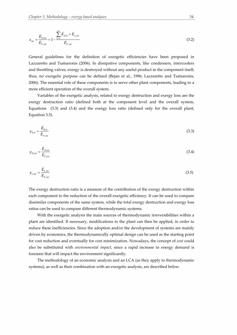
Chapter 3. Methodology – exergy based analyses 34
, ,, 1
, ,
1
n
D k L totP tot k
totF tot F tot
E EE
E E (3.2)
General guidelines for the definition of exergetic efficiencies have been proposed in
Lazzaretto and Tsatsaronis (2006). In dissipative components, like condensers, intercoolers
and throttling valves, exergy is destroyed without any useful product in the component itself;
thus, no exergetic purpose can be defined (Bejan et al., 1996; Lazzaretto and Tsatsaronis,
2006). The essential role of these components is to serve other plant components, leading to a
more efficient operation of the overall system.
Variables of the exergetic analysis, related to exergy destruction and exergy loss are the
exergy destruction ratio (defined both at the component level and the overall system,
Equations (3.3) and (3.4) and the exergy loss ratio (defined only for the overall plant,
Equation 3.5).
,,
,
D kD k
F tot
Ey
E (3.3)
,,
,
D totD tot
F tot
Ey
E (3.4)
,,
,
L totL tot
F tot
Ey
E (3.5)
The exergy destruction ratio is a measure of the contribution of the exergy destruction within
each component to the reduction of the overall exergetic efficiency. It can be used to compare
dissimilar components of the same system, while the total exergy destruction and exergy loss
ratios can be used to compare different thermodynamic systems.
With the exergetic analysis the main sources of thermodynamic irreversibilities within a
plant are identified. If necessary, modifications to the plant can then be applied, in order to
reduce these inefficiencies. Since the adoption and/or the development of systems are mainly
driven by economics, the thermodynamically optimal design can be used as the starting point
for cost reduction and eventually for cost minimization. Nowadays, the concept of cost could
also be substituted with environmental impact, since a rapid increase in energy demand is
foreseen that will impact the environment significantly.
The methodology of an economic analysis and an LCA (as they apply to thermodynamic
systems), as well as their combination with an exergetic analysis, are described below.

Chapter 3. Methodology – exergy based analyses 35
3.2.2 Exergy and economics
3.2.2.1 Economic analysis
Through an economic analysis, the economic feasibility of the construction and operation, as
well as the cost of the generated product of a facility can be estimated. To conduct an
economic analysis, different approaches can be used. In this thesis the total revenue requirement
(TRR) method is used (Bejan et al., 1996).
The most troublesome part of cost estimates for large power stations is the calculation of
the purchased equipment cost (PEC). A wide variety of data relating size and cost of different
types of components can be found in literature. However, most of these data consider
facilities much smaller than large‐scale power stations. To calculate costs of large‐scale
components using available data that consider reference equipment of different capacity, a
scaling exponent must be determined and used. This exponent, , is assumed to stay
constant within a given size range and it is usually lower than unity, expressing that a
percentage increase in the equipment cost is smaller than the percentage increase in capacity
(Bejan et al., 1996):
YY W
W
XC C
X (3.6)
Equation 3.6 is used to calculate the cost of purchased equipment (CY) of a new capacity (XY),
when a given cost (CW) at a certain capacity (XW) is known. In absence of specific cost
information an exponent value of 0.6 may be used.
When a base cost, CB, representing the cheapest possible design with basic materials at
low temperature and pressure is known, different factors depending on material,
temperature, pressure and design, ( , , ,m T p df f f f ) should be determined to estimate the fixed
capital investment (FCI). The cost of the module (i.e, the FCI) is then calculated as:
M B m T p d BMC C f f f f f . The bare module factor fBM considers any supporting equipment and
connections required, and it also includes all indirect costs related to the equipment. The PEC
is then calculated as a percentage of the FCI using specified modular factors (e.g., Guthrie,
1974).
When all costs have been calculated, they must be brought to the same reference year
that is used as the base year for all cost calculations (ref.). This is realized using cost indices
that are basically inflation indicators for both the reference year and the year of the
calculated, known costs (calc.):
.. .,
.
refref Y calc Y
calc
IndexC C
Index (3.7)
From the PEC, the cost rate kZ of each component k is estimated using Equation (3.8).

Chapter 3. Methodology – exergy based analyses 36
_ &
k k
tot
carrying charges O MZ PEC
PEC (3.8)
Here, τ represents the annual operating hours and O&M the operating and maintenance costs
of the plant. The carrying charges are calculated subtracting the fuel and O&M costs of the
plant from its TRR (Bejan et al., 1996). kZ is associated with both the investment cost (IC) and
the O&M costs of component k ( & IC O Mk k kZ Z Z ), but it is mainly determined by the
investment cost. The calculated cost rates are used as input for the exergoeconomic analysis.
3.2.2.2 Exergoeconomic analysis
An exergoeconomic analysis is an appropriate combination of an exergetic analysis with
economic principles. This is achieved through exergy costing, by which a specific cost c is
assigned to each exergy stream of the plant. The specific cost of stream i, ic , multiplied by the
exergy of the same stream, iE , provides the cost rate iC , associated with stream i:
i i iC c E (3.9) To perform an exergoeconomic analysis on a plant, cost balances are stated at the component
level resulting in a system of balance equations. For example, the cost balance of component k
is stated as follows:
, ,1 1
0
l m
i k j k ki j
C C Z (3.10)
Here, ,1
l
i ki
C is the sum of the cost rates associated with the l steams entering component k
and ,1
m
j kj
C is the sum of the cost rates associated with the m streams leaving component k.
In the system of balance equations, when the number of unknown stream costs is larger
than the number of equations stated, auxiliary statements are required. For each component,
streams entering are assumed to be known, while streams leaving the component are
unknown. When the number of the outgoing exergy streams of a component is higher than
one (m > 1), m‐1 auxiliary equations are needed. The P‐principle (on the product side) and the
F‐principle (on the fuel side) are used to determine the auxiliary equations (Lazzaretto and
Tsatsaronis, 2006). The P‐principle states that the cost per unit of exergy is supplied to all
streams that belong to the definition of the product of the component at the same cost. The F‐
principle states that the cost, associated with the exergy removed from a considered
component, has the same specific cost as the exergy supplied to the upstream components.
When the necessary balance equations are stated and solved, the exergoeconomic
evaluation follows. Through the evaluation, iterative steps to improve and finally optimize

Chapter 3. Methodology – exergy based analyses 37
the considered system are revealed. An important outcome of the exergoeconomic analysis is
the relation of exergy destruction with costs:
, , ,D k F k D kC c E (3.11)
where, ,F kc is the specific cost of fuel of component k.
The calculation of the cost of exergy destruction facilitates the evaluation of plant
components and allows comparison between cost of exergy destruction and investment cost.
The components are first ranked and evaluated based on their total costs ,D k kC Z . The
higher the costs are, the more significant the effect of the component to the overall plant. The
contribution of the capital cost, kZ , to the sum of costs is expressed by the exergoeconomic
factor kf , defined by Equation (3.12).
k,Dk
kk
CZ
Zf
(3.12)
The exergoeconomic factor depends on the operation of each component. However, for
each component type, there are some common value ranges that usually apply (lower than
55% for HXs; 35‐75% for compressors/turbines; higher than 90% for pumps). High values of
the factor f suggest a reduction in the investment costs, while low values of f suggest a
reduction in the incurred irreversibilities. Depending on the calculated values, trade‐offs
between exergy destruction and investment costs are suggested. The goal is to improve the
overall plant from both thermodynamic and economic viewpoints.
Another important variable of the exergoeconomic evaluation is the relative cost
difference, kr . For a given component k, the difference between the specific cost of product,
,P kc , and the specific cost of fuel, ,F kc , depends on the cost of exergy destruction, ,D kC , and
the related kZ .
, , ,
, , ,
P k F k D k kk
F k F k P k
c c C Zr
c c E (3.13)
Information about compromises between the cost of exergy destruction and the
investment cost of components, resulting from the exergoeconomic evaluation, can be used
for the iterative design improvement of the plant. The objective is to reduce the cost
associated with the product of the overall plant.

Chapter 3. Methodology – exergy based analyses 38
3.2.3 Exergy and environmental impacts
3.2.3.1 Life cycle assessment
In analogy to the economic analysis used to calculate costs, an LCA is used to assess the
environmental impact associated with a product over its lifetime (Meyer et al., 2009). It is
carried out following the guidelines of international standard approaches (ISO 14004).
Figure 3.1: General structure of the Eco‐indicator 99 LCIA method (Source: Goedkoop and Spriensma,
2000)
The quantification of environmental impacts caused by depletion and emissions of a
natural resource can be carried out using different life cycle impact assessment (LCIA) methods.
The damage‐oriented impact analysis method Eco‐indicator 99 is considered here (Goedkoop
and Spriensma, 2000). Eco‐indicator 99 defines three categories of damage: (1) damage to
human health, (2) damage to the ecosystem and (3) depletion of resources. After calculating
the environmental effects of the different categories, the values are optionally normalized,
weighted and the result is expressed in Eco‐indicator points (Pts). Higher values of the Eco‐
indicator are associated with higher damage. Depending on the attitude and perspective of
different societies, there is a weighting per perspective represented by three Archetypes:
Hierarchists keep a balance between short and long‐term perspectives and take
environmental damages into account based on consensus.
Egalitarians weigh the effect on future generations and take all possible effects
into account, even with minimal scientific proof.
Individualists focus on the present, neglecting long‐term effects and take only
proven effects into account.
The archetype of the hierarchists has been adopted in this thesis.
The standard Eco‐indicator 99 inventory values are available for the production and
processing of a large number of materials, for transport processes, for disposal scenarios, etc.
The impact is calculated with reference to the annual environmental impact of a European
inhabitant. The scale is chosen in such a way that the value of 1 Point is representative for one
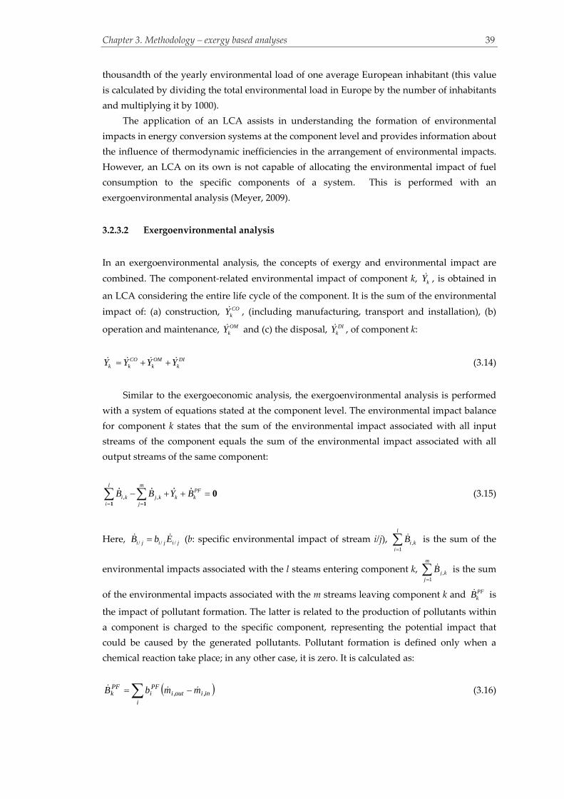
Chapter 3. Methodology – exergy based analyses 39
thousandth of the yearly environmental load of one average European inhabitant (this value
is calculated by dividing the total environmental load in Europe by the number of inhabitants
and multiplying it by 1000).
The application of an LCA assists in understanding the formation of environmental
impacts in energy conversion systems at the component level and provides information about
the influence of thermodynamic inefficiencies in the arrangement of environmental impacts.
However, an LCA on its own is not capable of allocating the environmental impact of fuel
consumption to the specific components of a system. This is performed with an
exergoenvironmental analysis (Meyer, 2009).
3.2.3.2 Exergoenvironmental analysis
In an exergoenvironmental analysis, the concepts of exergy and environmental impact are
combined. The component‐related environmental impact of component k, kY , is obtained in
an LCA considering the entire life cycle of the component. It is the sum of the environmental
impact of: (a) construction, COkY , (including manufacturing, transport and installation), (b)
operation and maintenance, OMkY and (c) the disposal, DI
kY , of component k:
CO OM DIk k k kY Y Y Y (3.14)
Similar to the exergoeconomic analysis, the exergoenvironmental analysis is performed
with a system of equations stated at the component level. The environmental impact balance
for component k states that the sum of the environmental impact associated with all input
streams of the component equals the sum of the environmental impact associated with all
output streams of the same component:
, ,
l mPF
i k j k k ki j
B B Y B
1 1
0 (3.15)
Here, / / /i j i j i jB b E (b: specific environmental impact of stream i/j), ,1
l
i ki
B is the sum of the
environmental impacts associated with the l steams entering component k, ,1
m
j kj
B is the sum
of the environmental impacts associated with the m streams leaving component k and PFkB is
the impact of pollutant formation. The latter is related to the production of pollutants within
a component is charged to the specific component, representing the potential impact that
could be caused by the generated pollutants. Pollutant formation is defined only when a
chemical reaction take place; in any other case, it is zero. It is calculated as:
i
in,iout,iPFi
PFk mmbB (3.16)

Chapter 3. Methodology – exergy based analyses 40
where, inm and outm are the mass flow rates of pollutants entering and exiting component k,
respectively. The pollutant streams that are taken into account here include: CO, CO2, CH4
and NOX.
When auxiliary equations need to be formulated, to make the number of the unknowns
equal to the number of equations, the same principles are valid as for the exergoeconomic
analysis.
The environmental impact of the exergy destruction is calculated as:
, , , D k F k D kB b E (3.17)
Here, bF,k is the specific environmental impact of the fuel provided to component k. ,
D kB can
then be compared to the component‐related impact of component k, kY . This is the first step
in evaluating the plant components, by revealing those with the highest effect on the overall
plant.
The exergoenvironmental analysis not only identifies the components with the highest
environmental impact, but it also reveals the possibilities for improvement, in order to
decrease the environmental impact of the overall plant. These improvement possibilities can
be identified through the sum of the component‐related environmental impact and the
impact of exergy destruction, , k D kY B , the exergoenvironmental factor, ,b kf , and the relative
environmental impact difference, ,b kr .
kb,k
k D,k
Yf =
Y B
(3.18)
,,
,
F,k P,k D k kb k
F,k F,k P k
b b B Yr
b b E
(3.19)
With the exergoenvironmental factor, the contribution of the component‐related impact,
kY , to the total environmental impact, , k D kY B is expressed at the component level. In theory,
when the value of ,b kf is relatively high, kY is dominant, whereas when the value of ,b kf is
low, exergy destruction is dominant. Thus, the higher the exergoenvironmental factor, the
higher the influence of the component‐related impact on the overall performance of the plant.
In practice, the results of the exergoenvironmental factor differ from those of the
exergoeconomic factor significantly: the component‐related impact is very low when
compared to the impact associated with the operation of the plant (exergy destruction).
Therefore, the values of ,b kf are lower than 1% for the majority of the components. This is
discussed in more detail in Chapter 4, where the results of the analyses are presented.
The environmental impact difference of component k, ,b kr , depends on the impact of its
exergy destruction and its component‐related impact. Thus, it is an indicator of the reduction
potential of the component. After the calculation and evaluation of the mentioned variables,

Chapter 3. Methodology – exergy based analyses 41
design changes are suggested, in order to reduce the environmental impact associated with
the product of the overall process.
3.3 Advanced exergy‐based analyses
With conventional exergy‐based analyses, the locations, magnitudes and causes of
irreversibilities, costs and environmental impacts are identified, and a general direction for
improvement is indicated. However, none of the conventional analyses are able to reveal
interactions among plant components or to estimate the real potential for improvement.
Without consideration of component interactions, optimization strategies can be misguided,
especially when complex systems with a large number of mutually‐affected components are
considered. Advanced exergy‐based analyses attempt to address this shortcoming.
Part of the exergy destruction, cost and environmental impact of a system can be
avoided with structural modifications, reduction of the investment costs/environmental
impacts or efficiency improvements of individual components. Exergy destruction, costs and
environmental impacts that can be avoided through technically feasible design and/or
operational improvement are considered avoidable, (AV). AV quantities play the main role in
the determination of improvement steps, as well as the estimation of the improvement
potential of a system. The remaining exergy destruction, costs and environmental impacts,
associated with physical, technological and economic constraints, that cannot be avoided, are
considered unavoidable, (UN). Additionally, exergy destruction, costs and environmental
impacts can be separated depending on their source: if they are incurred by component
interactions, they are exogenous (EX), while if they stem from the operation of the component
itself, they are endogenous (EN). Using the endogenous and exogenous quantities, interactions
among components and improvement alternatives are identified. Furthermore, the avoidable
and unavoidable estimates are further split into their endogenous and exogenous parts. A
schematic example of the paths to split irreversibilities is shown in Figure 3.2. The same
process is applied to costs and environmental impacts.
Figure 3.2: Options for splitting the exergy destruction in an advanced exergetic analysis (Source:
Morosuk and Tsatsaronis, 2008b)
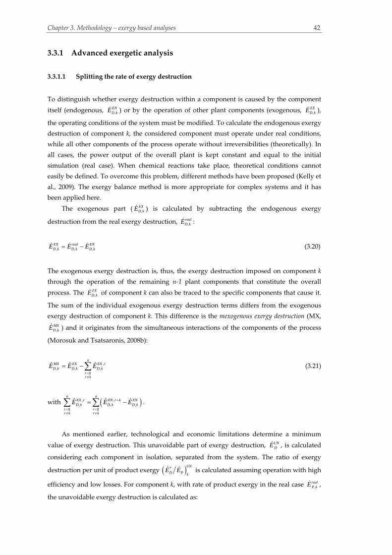
Chapter 3. Methodology – exergy based analyses 42
3.3.1 Advanced exergetic analysis
3.3.1.1 Splitting the rate of exergy destruction
To distinguish whether exergy destruction within a component is caused by the component
itself (endogenous, ,END kE ) or by the operation of other plant components (exogenous, ,
EXD kE ),
the operating conditions of the system must be modified. To calculate the endogenous exergy
destruction of component k, the considered component must operate under real conditions,
while all other components of the process operate without irreversibilities (theoretically). In
all cases, the power output of the overall plant is kept constant and equal to the initial
simulation (real case). When chemical reactions take place, theoretical conditions cannot
easily be defined. To overcome this problem, different methods have been proposed (Kelly et
al., 2009). The exergy balance method is more appropriate for complex systems and it has
been applied here.
The exogenous part ( ,EXD kE ) is calculated by subtracting the endogenous exergy
destruction from the real exergy destruction, ,realD kE :
, , ,EX real END k D k D kE E E (3.20)
The exogenous exergy destruction is, thus, the exergy destruction imposed on component k
through the operation of the remaining n‐1 plant components that constitute the overall
process. The ,EXD kE of component k can also be traced to the specific components that cause it.
The sum of the individual exogenous exergy destruction terms differs from the exogenous
exergy destruction of component k. This difference is the mexogenous exergy destruction (MX,
,MXD kE ) and it originates from the simultaneous interactions of the components of the process
(Morosuk and Tsatsaronis, 2008b):
,, , ,
1
nMX EX EX rD k D k D k
rr k
E E E (3.21)
with , ,, , ,
1 1
n nEX r EN r k END k D k D k
r rr k r k
E E E .
As mentioned earlier, technological and economic limitations determine a minimum
value of exergy destruction. This unavoidable part of exergy destruction, UNDE , is calculated
considering each component in isolation, separated from the system. The ratio of exergy
destruction per unit of product exergy * UN
D P kE E is calculated assuming operation with high
efficiency and low losses. For component k, with rate of product exergy in the real case ,realP kE ,
the unavoidable exergy destruction is calculated as:

Chapter 3. Methodology – exergy based analyses 43
*
, ,
UN
UN real DD k P k
P k
EE E
E (3.22)
When the unavoidable part of the exergy destruction within component k is known, the
avoidable part is obtained with Equation (3.23):
, , ,AV real UND k D k D kE E E (3.23)
For dissipative components no rate of product exergy can be defined, thus no distinction
between avoidable and unavoidable exergy destruction has been made.
3.3.1.2 Splitting the avoidable and unavoidable rates of exergy destruction into
endogenous and exogenous parts
The unavoidable endogenous and exogenous exergy destruction ,,
UN END kE and ,
,UN EXD kE within
component k is calculated with Equations (3.24) and (3.25):
*,
, ,
UN
UN EN EN DD k P k
P k
EE E
E (3.24)
, ,
, , ,UN EX UN UN END k D k D kE E E (3.25)
The avoidable endogenous and exogenous exergy destruction ,,
AV END kE and ,
,AV EXD kE is then
calculated by subtracting the corresponding unavoidable part from the total endogenous and
exogenous exergy destruction, respectively:
, ,
, , ,AV EN EN UN END k D k D kE E E (3.26)
, ,
, , ,AV EX EX UN EXD k D k D kE E E (3.27)
3.3.1.3 Calculating the total avoidable exergy destruction
In general, high avoidable exergy destruction reveals high improvement potential for a
component. However, it is possible that a component has relatively low avoidable exergy
destruction, but relatively high total avoidable exogenous exergy destruction (exergy
destruction caused by the component both within itself and to the other components of the
system). Thus, an evaluation should take into account all data available and the conclusions
should be adjusted accordingly. To facilitate the identification of the real improvement
potential of plant components, the total amount of avoidable exergy destruction caused by
each component k is defined (Morosuk and Tsatsaronis, 2008b):

Chapter 3. Methodology – exergy based analyses 44
, , , ,, , ,
1
nAV AV EN AV EX kD k D k D r
rr k
E E E
(3.28)
Here, , ,,
1
n
AV EX kD r
rr k
E is the sum of the avoidable exergy destruction caused by component k
within the remaining n‐1 plant components. Each part of this sum is calculated for each
component r separately, via the unavoidable exogenous exergy destruction. The unavoidable
exogenous exergy destruction is calculated through the unavoidable endogenous exergy
destruction of each component r, when r and k operate under real conditions (Morosuk and
Tsatsaronis, 2008b),:
*, , ,
, ,
UN
UN EN r k EN r k DD r P r
P r
EE E
E (3.29)
,
, EN r k
P rE is the PE of component r, when components r and k operate under real conditions
and all remaining components operate under theoretical conditions. The unavoidable
exogenous exergy destruction in component r due to component k, , ,,
UN EX kD rE , is calculated as:
, , , , ,, , ,
UN EX k UN EN r k UN END r D r D rE E E (3.30)
Finally, the avoidable exogenous exergy destruction of component r caused by component k,
is found by subtracting the unavoidable exogenous exergy destruction from the total
exogenous exergy destruction caused to r by component k:
, , , , ,
, , , AV EX k EX k UN EX kD r D r D rE E E (3.31)
3.3.2 Advanced exergoeconomic analysis
3.3.2.1 Splitting the cost rates of investment and exergy destruction
Similar to exergy destruction, the endogenous and exogenous parts of investment cost and
cost of exergy destruction are the parts related to internal operating conditions and to
component interactions, respectively. Moreover, depending on whether the costs can be
avoided or not, they can be split into avoidable and unavoidable parts, respectively. All
equations used for these calculations are shown in Table 3.1.

Chapter 3. Methodology – exergy based analyses 45
3.3.2.2 Calculating the total rates of avoidable costs
To identify the real potential for improving plant components, the sum of both avoidable
costs associated with exergy destruction and avoidable investment costs are calculated at the
component level:
, , , ,, , ,
1
nAV AV EN AV EX kD k D k D r
rr k
C C C
(3.32)
, , , ,
1
nAV AV EN AV EX kk k r
rr k
Z Z Z
(3.33)
, ,,
1
nAV EX kD r
rr k
C
and , ,
1
nAV EX kr
rr k
Z
are the total avoidable cost rates associated with the exogenous
exergy destruction and investment cost of component r, respectively, caused by component k.
The term related to the avoidable exogenous investment cost is calculated for each
component r separately, via the unavoidable exogenous investment cost of the component
caused by component k, , ,UN EX krZ :
, , , , ,AV EX k EX k UN EX kr r rZ Z Z (3.34)
The unavoidable exogenous part of the cost is calculated through the unavoidable
endogenous cost, ,UN ENrZ :
, , , , ,UN EX k UN EN r k UN ENr r rZ Z Z (3.35)
where, , , ,, ,
UN
UN EN r k EN r kD r P r
P r
ZZ E
E, with ,
, EN r k
P rE equivalent to ,
P rE , when components r and k
operate under real conditions and all remaining components operate theoretically.
To compare the avoidable cost of exergy destruction with the avoidable investment cost,
the cost of exergy destruction must be split into its sources, as well. The avoidable exogenous
cost of exergy destruction is calculated with Equation (3.36):
, , , ,, , , AV EX k real AV EX k
D r F r D rC c E (3.36)
where, , ,,
AV EX kD rE has been calculated using Equation (3.31).
The total cost, upon which the performance of a component is evaluated, is the sum of
the avoidable cost rates of exergy destruction and investment.

Chapter 3. Methodology – exergy based analyses 46
Table 3.1: Splitting the costs
TERM Definition
of cost rate Cost rate of investment, kZ , and exergy
destruction, ,
D kC , (of component k)
Comments
Endogenous
(ENZ ,
ENDC )
Cost rate within component k associated with
the operation of the component itself
,
k
real
EN ENP k
P k
ZZ E
E
, , , EN real END k F k D kC c E
, EN
P kE : Rate of product exergy of component k when the remaining components operate theoretically
realPE and realZ : Rate of product exergy and investment cost in the real case
,realF kc : Average cost per unit of fuel exergy provided to component k in the real case
Exogenous
(EXZ ,
EXDC )
Mexogenous
(MXZ ,
MXDC )
Cost rate within component k caused by the
remaining components
Difference between exogenous and sum of
split exogenous cost rates for component k,
caused by simultaneous interactions between
the component and the remaining
components of the plant
k
EX real ENk kZ Z Z
, , , EX real END k D k D kC C C
,
1
nMX EX EX rk k k
rr k
Z Z Z
,, , ,
1
nMX EX EX rD k D k D k
rr k
C C C
, ,
1 1
n nEX r EN r k ENk k k
r rr k r k
Z Z Z , with , ,
,
real
EN r k EN r k kk P
P k
ZZ E
E
, ,, , ,
1 1
n nEX r EN r k END k D k D k
r rr k r k
C C C , with , ,
, , , EN r k real EN r k
D k F k D kC c E
Unavoidable
(UNZ ,
UNDC )
Cost rate that cannot be avoided
UN
UN realk kreal
k
PECZ Z
PEC for HXs
% of realkZ for other components
UNkZ : Unavoidable investment cost rate, i.e., minimum cost associated with component k. For each heat
exchanger a new simulation of the component in isolation, operating with low effectiveness and high
irreversibilities, is required. For other components, part of their realZ is chosen as unavoidable.
UNkPEC : Purchased equipment cost of component k, calculated at the unavoidable conditions
, , , UN real UN
D k F k D kC c E UNDE : Unavoidable part of exergy destruction rate (calculated in an advanced exergetic analysis with
most favorable operating conditions that result in the lowest possible exergy destruction).
Avoidable Cost rate that can be avoided AV real UNk k kZ Z Z
(AVZ ,
AVDC ) , , , AV real UN
D k D k D kC C C
Unavoidable Endogenous
(,UN ENZ ,
,UN ENDC )
Unavoidable cost rate within component k
associated with the operation of the
component itself
,
*,
k
P k
UN
UN EN EN
P k
ZZ E
E
* UN UN
realP Pk k
Z Z
E E
Unavoidable Exogenous
(,UN EXZ ,
,UN EXDC )
Unavoidable cost rate within component k
caused by the remaining components
, ,, , , UN EN real UN EN
D k F k D kC c E
, , k
UN EX UN UN ENk kZ Z Z
, ,, , , UN EX UN UN EN
D k D k D kC C C
,UN ENDE : Unavoidable endogenous part of exergy destruction rate (calculated in an advanced exergetic
analysis)
Avoidable Endogenous
(,AV ENZ ,
,AV ENDC )
Avoidable cost rate within component k
associated with the operation of the
component itself
, , k k k
AV EN EN UN ENZ Z Z
, ,, , , AV EN EN UN EN
D k D k D kC C C
Avoidable Exogenous
(,AV EXZ ,
,AV EXDC )
Avoidable cost rate within component k
caused by the remaining components
, , k
AV EX EX UN EXk kZ Z Z
, ,, , , AV EX EX UN EX
D k D k D kC C C
Chapter 3. M
ethodology – exergy‐based analyses 46
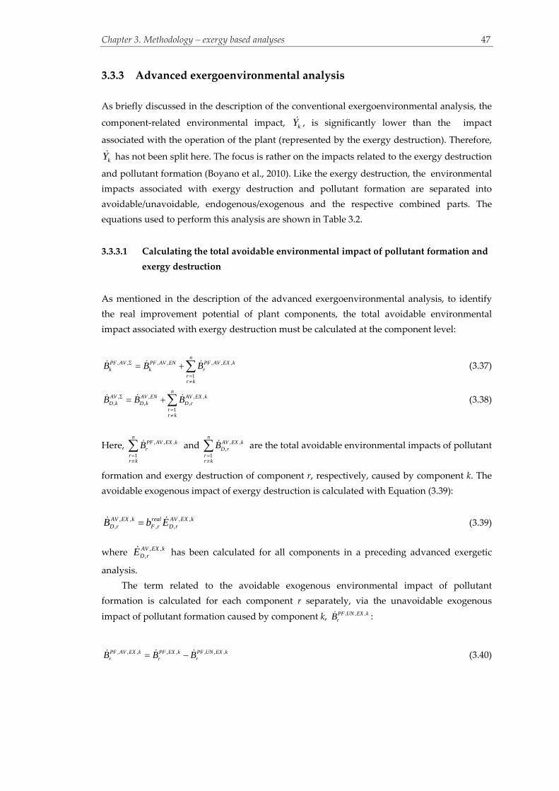
Chapter 3. Methodology – exergy based analyses 47
3.3.3 Advanced exergoenvironmental analysis
As briefly discussed in the description of the conventional exergoenvironmental analysis, the
component‐related environmental impact, kY , is significantly lower than the impact
associated with the operation of the plant (represented by the exergy destruction). Therefore,
kY has not been split here. The focus is rather on the impacts related to the exergy destruction
and pollutant formation (Boyano et al., 2010). Like the exergy destruction, the environmental
impacts associated with exergy destruction and pollutant formation are separated into
avoidable/unavoidable, endogenous/exogenous and the respective combined parts. The
equations used to perform this analysis are shown in Table 3.2.
3.3.3.1 Calculating the total avoidable environmental impact of pollutant formation and
exergy destruction
As mentioned in the description of the advanced exergoenvironmental analysis, to identify
the real improvement potential of plant components, the total avoidable environmental
impact associated with exergy destruction must be calculated at the component level:
, , , , , , ,
1
nPF AV PF AV EN PF AV EX kk k r
rr k
B B B
(3.37)
, , , ,, , ,
1
nAV AV EN AV EX kD k D k D r
rr k
B B B
(3.38)
Here, , , ,
1
nPF AV EX kr
rr k
B
and , ,,
1
nAV EX kD r
rr k
B
are the total avoidable environmental impacts of pollutant
formation and exergy destruction of component r, respectively, caused by component k. The
avoidable exogenous impact of exergy destruction is calculated with Equation (3.39):
, , , ,, , ,
AV EX k real AV EX kD r F r D rB b E (3.39)
where , ,,
AV EX kD rE has been calculated for all components in a preceding advanced exergetic
analysis.
The term related to the avoidable exogenous environmental impact of pollutant
formation is calculated for each component r separately, via the unavoidable exogenous
impact of pollutant formation caused by component k, , , ,PF UN EX krB :
, , , , , , , ,PF AV EX k PF EX k PF UN EX kr r rB B B (3.40)

Chapter 3. Methodology – exergy based analyses 48
The unavoidable exogenous environmental impact of pollutant formation is calculated
through its unavoidable endogenous impact, , ,PF UN ENrB :
, , , , , , ,PF UN EX k PF UN EN r k UN ENr r rB B B (3.41)
, , , ,, ,
UNPFPF UN EN r k EN r kD r P r
P r
BB E
E, with ,
, EN r k
P rE equivalent to the ,
P rE , when components r and k
operate under real conditions and all remaining components operate theoretically.
The total avoidable environmental impacts (Equations 3.37 and 3.38) reveal the
components with the largest influence on the overall plant. Actions to improve their
operation should lead to an improvement of the impact of the plant as a whole.

Chapter 3. Methodology – exergy based analyses
49
Table 3.2: Splitting the environmental impacts
TERM Definition
of environmental impact
Environmental impact of pollutant
formation, k
PFB and exergy
destruction, ,
D kB (for component k)
Comments
Endogenous
(,PF EN
kB , ,END kB )
Impact within component k associated with the
operation of the component itself
,, , ENPF EN PF
k i i out i ini
B b m m
, , , EN real END k F k D kB b E
PFib : Specific pollutant formation (varies depending on the pollutant)
, , EN
i out i inm m : mass flow difference of pollutant i, between outlet and inlet in the endogenous case
,realF kb : Average specific environmental impact per unit of fuel exergy of component k in the real case
Exogenous
(,PF EX
kB , ,EXD kB )
Mexogenous
(,PF MX
kB , ,MXD kB )
Impact associated with component k caused by the
remaining components
Difference between exogenous and sum of split
exogenous impacts for component k, caused by
simultaneous interactions between the component
and the remaining components of the plant
, , , PF EX PF real PF ENk k kB B B
, , , EX real END k D k D kB B B
,, , ,
1
nMX EX EX rD k D k D k
rr k
B B B
, ,, , ,
1 1
n nEX r EN r k END k D k D k
r rr k r k
B B B , with , ,
, , , EN r k real EN r k
D k F k D kB b B
Unavoidable
(,PF UN
kB , ,UND kB )
Impact that cannot be avoided ,, , PF UN PF
k i i out i ini
B b m m
, , , UN real UND k F k D kB b E
,PF UNkB : The unavoidable environmental impact of pollutant formation rate includes all emissions of
2CO when complete combustion takes place ( i: 2CO )
UNDE : Unavoidable part of exergy destruction rate (calculated in an advanced exergetic analysis with
most favorable operating conditions that result in the lowest possible exergy destruction).
Avoidable
(,PF AV
kB , ,AVD kB )
Impact that can be avoided ,,
X X
PF AV PFk NO NO outB b m
, , , AV real UND k D k D kB B B
,PF AVkB : NOX emissions that can be avoided assuming, for example, different excess air fraction ( λ)
Unavoidable
Endogenous
(, ,PF UN EN
kB ,,
,UN END kB )
Unavoidable impact associated with component k
caused by the operation of the component itself
*
,
, ,
,
k
P k
UNPF
PF UN EN EN k
P k
BB E
E
, ,, , , UN EN real UN EN
D k F k D kB b E
* ,
UNPF PF UN
realP P kk
B B
E E
Unavoidable Exogenous
(, ,PF UN EX
kB ,,
,UN EXD kB )
Unavoidable impact within component k caused
by the remaining components
, , , , , k
PF UN EX PF UN PF UN ENk kB B B
, ,, , , UN EX UN UN EN
D k D k D kB B B
Avoidable Endogenous
(, ,PF AV EN
kB ,,
,AV END kB )
Avoidable impact within component k caused by
the operation of the component itself
, , , , , k k k
PF AV EN PF EN PF UN ENB B B
, ,, , , AV EN EN UN EN
D k D k D kB B B
Avoidable Exogenous
(, ,PF AV EX
kB ,,
,AV EXD kB )
Avoidable impact within component k caused by
the remaining components
, , , , , k
PF AV EX PF AV PF AV ENk kB B B
, ,, , , AV EX EX UN EX
D k D k D kB B B
Chapter 3. M
ethodology – exergy‐based analyses 49

Chapter 3. Methodology – exergy based analyses
50

Chapter 4. Application of the exergy‐based analyses to the plants 51
4. Application of the exergy‐based analyses to the plants
This chapter includes details and particularities of the applied methods and the obtained
results. Information about the application of the conventional exergy‐based analyses can be
found in Appendix B.2. Selected results for the considered plants of each method are
presented in the respective sections and summarized in Table 4.5. Results for selected plant
components are shown in Tables 4.6‐4.13 (end of section 4.1), while analytical results are
presented in Appendix A.
4.1 Conventional exergy‐based analyses
4.1.1 Exergetic analysis
All of the plants are provided with the same amount of fuel. Thus, the derived rate of product
exergy ( ,P totE ) depends on the operating characteristics of each plant and the requirements of
each CO2 capture technology. Selected results of the analysis are presented in Table 4.1.
Table 4.1: Selected results of the exergetic analysis
Ref. Plant AZEP
85
AZEP
100
CLC
Plant MEA‐0.2 S‐GRAZ
ATR
PlantMEA‐0
MSR
Plant
Simple oxy‐
fuel Plant
tot (%) 56.5 53.4 51.7 51.5 48.4 48.0 46.5 45.8 45.8 42.7
,P totE (MW) 412.5 389.9 377.5 376.0 353.8 352.0 339.8 334.6 334.6 313.4
,F totE (MW) 300.4 313.4 320.7 307.4 349.1 349.3 358.1 368.3 338.7 388.7
,L totE (MW) 17.6 27.2 32.5 47.3 27.6 31.9 32.7 27.7 57.3 31.1
,D toty (%) 41.1 42.9 43.9 42.1 47.8 47.6 49.0 50.4 46.4 53.0
The reference plant performs with an exergetic efficiency of 56.5%. Of the plants that
include CO2 capture, the AZEP 85 achieves the best performance (53.4%), followed by the
AZEP 100 (51.7%) and the CLC plant (51.5%). MEA‐0.21 is ranked fourth (48.4%), while the S‐
Graz cycle is ranked fifth (48.0%), followed by the ATR plant (46.5%). MEA‐0 and the MSR
plant operate with a similar efficiency (45.8%) and, therefore, occupy the same ranking place
1 0 and 0.2 stand for the assumed lean sorbent CO2 loading (0 or 0.2 mol CO2/mol MEA). See also section 2.3.2.

Chapter 4. Application of the exergy‐based analyses to the plants 52
(the efficiency of the MSR plant is slightly lower than that of MEA‐0). Lastly, the lowest
efficiency is found for simple oxy‐fuel plant (42.7%). The results of MEA‐0.2 agree better with
published work (Rubin and Rao, 2002). Therefore, although MEA‐0 will some times be used
for comparison purposes, MEA‐0.2 is considered as the main representative plant for
chemical absorption. If not otherwise stated, MEA plant refers to MEA‐0.2.
The three most efficient plants (AZEP 85, AZEP 100 and CLC plant) are oxy‐fuel
concepts. This indicates that this general approach is relatively promising for CO2 capture, as
long as current implementation challenges, related to their operation and component
feasibility, are met. When compared to the reference plant, these plants result in a relatively
small reduction in the exergetic efficiency of about five percentage points. Although the total
rate of exergy destruction ( ,D totE ) in the CLC plant is lower by 6‐13 MW than that of the
AZEPs, the rate of product exergy of both AZEPs is found to be higher. With the same ,F totE
and lower ,D totE , the lower ,P totE of the CLC plant is explained by its larger rate of exergy loss
( ,L totE ). Indeed, the exergy loss of the AZEP 100 and AZEP 85 is 32.5 and 27.3 MW (4.5 and
3.7% of the ,F totE ), respectively, while in the CLC plant it is 47.3 MW (6.5% of the ,F totE ). The
higher exergy loss in the latter is a result of the assumed 2% non‐reacted methane (see also
section 2.3.7). The lower exergy loss of the AZEP 85 is smaller than that of the AZEP 100,
because of the reduced mass flow rates of (1) the captured CO2, (2) the MCM working fluids
and (3) the GT system, and the smaller mass flow rate and lower temperature of the exhaust
gases. The combination of relatively low exergy destruction and loss in the AZEP 85 results in
higher net power output, i.e. higher exergetic efficiency.
The large difference between the simple oxy‐fuel concept and the S‐Graz cycle results
from a combination of factors. In the S‐Graz, (1) additional power is produced in the low
pressure GT (GT3), (2) the exergy destruction within the single‐pressure level HRSG is lower
when compared to that of the three‐pressure level HRSG of the simple oxy‐fuel plant, (3) the
water separated through gas condensation is recycled and reused in the plant and (4) steam is
added at different pressure levels of the GT system, increasing the expanding mass flow and
allowing a low condenser working pressure. All of these points contribute to an increase in
the net power output of the S‐Graz cycle. The S‐Graz cycle performs with lower efficiency
when compared to the CLC plant and the AZEP concepts, mainly because of the large power
demand of its recycle compressors.
The two pre‐combustion plants perform with relatively low efficiencies. The justification
of this result for the ATR plant is that it combines two costly CO2 capture methods: chemical
absorption and fuel de‐carbonization. Chemical absorption requires large amounts of thermal
energy, while the de‐carbonization process includes a, strongly endothermic, reforming
reaction that is fueled by a supplementary fuel burning. The low effectiveness of the MSR
plant is explained by its high rate of exergy loss. The MSR plant presents the highest rate of
exergy loss among all of the plants (7.8% of the ,F totE ), due to the relatively high exergy rate
of the stream exhausted to the environment.
The MEA plant results in an efficiency of 8 percentage points lower than that of the
reference plant, with an exergy loss similar to that of the AZEP 85 because of the low exergy

Chapter 4. Application of the exergy‐based analyses to the plants 53
rate of the exhaust gases. However, the MEA plant presents a lower overall efficiency of 3‐5
percentage points when compared to the three most efficient oxy‐fuel plants. The relatively
low penalty of the three oxy‐fuel plants stems from their more efficient combustion processes,
the additional power produced in the additional expander (GT2 in Figures A.2.1, A.3.1 and
A.5.1), and the additional HRSG (SH II, EV II, EC II) that increases heat‐recovery.
As expected, the main exergy destruction in all of the plants occurs within their chemical
reactors (CC, CLC reactors, DB), caused by the high irreversibilities incurred there. When the
reactants are preheated, the thermodynamic irreversibilities within the reactors decrease
significantly. The combustion process is realized more efficiently in the AZEPs and the CLC
plant resulting in an exergy destruction ratio 100,
AZEPD CCy / 85
, AZEPD CC DBy / ,
CLCD reactorsy 12‐18% lower (the
best case being the AZEP 100), when compared to the reference plant. Furthermore, in the
AZEP 100 the exergy destruction ratio of the combustion process is lower than that of the
AZEP 85, which includes both a CC and a DB. This is related to the lower exergetic efficiency
of the DB. The exergy destruction within the CC of the MEA plant is exactly the same as that
of the reference plant, because the GT systems of the two plants are identical.
Apart from the GT system, with a dominant influence due to its high values of ,D kE ,
other components appear to be equally important. In the CAU of the MEA and ATR plants, 4‐
6%, and in the ASUs of the simple oxy‐fuel plant and the S‐Graz cycle, 5‐6% of the plants’
,F totE is destroyed. The CAU in the MEA plant, and the ASUs in the S‐Graz and simple oxy‐
fuel plants have the second highest values of exergy destruction among the plant
components. In the ATR plant, the second highest exergy destruction is found within the
ATR, followed by the CAU. In the remaining plants, the CC is followed by the expander and
the compressor of the GT system (GT1 and C1) in descending order of exergy destruction.
The high‐pressure level of the HRSG (HPHRSG) is the most important part of the HRSG in all
of the plants, followed by its respective low‐pressure level part (LPHRSG). Lastly, the LPST
and the additional ST used to drive the CO2 compressors (ST4) also present relatively
significant values of exergy destruction. The CO2 compression unit is responsible for
approximately 3% of the ,F totE in the AZEPs, the CLC and MSR plants, 2% in the MEA,
simple oxy‐fuel and S‐Graz plants and 1% in the ATR plant.
In general, the AZEPs and the CLC plant perform comparably, resulting in similar
component efficiencies. While on close inspection, the majority of the components in the
AZEPs operate slightly more efficiently than those in the CLC plant, the total exergy
destruction ratio in both of the AZEPs is higher because of the higher exergy destruction
within the MCM reactors, HRSG II and ST4. ST4 presents a higher exergy destruction ratio in
the AZEPs, because it covers both the CO2 compression unit and the recycle compressor of the
plants. HRSG II of the AZEPs has higher exergy destruction, because of the larger steam mass
flows, which are a result of the larger amount of available thermal energy in the CO2 stream.
The CO2 compression unit in the AZEP 100 operates with larger CO2 mass flow, therefore
requiring a higher mass flow of cooling water that results in higher exergy destruction
compared to the AZEP 85. Between the AZEP 100 and the CLC plant, the CO2 mass flow
differences are significantly smaller and are caused by the lower amount of CH4 reacting in
the latter.

Chapter 4. Application of the exergy‐based analyses to the plants 54
The subsequent analyses of sections 4.1.2 and 4.1.3 have been applied to the reference
plant and four plants incorporating CO2 capture: the MEA plants (MEA‐0 and MEA‐0.2), the
CLC plant, the AZEP 100 and the AZEP 85. The chemical absorption technique has been
chosen as representative of the most conventional CO2 capture method, whereas the three
oxy‐fuel plants have been chosen due to their high efficiencies, when compared to the
alternative technologies.
4.1.2 Exergy and economics
4.1.2.1 Results of the economic analysis
The investment cost of the reference plant is calculated to be 213 € million (Table 4.2). The
largest cost increase is estimated for the AZEP 100 (414 € million), followed by the AZEP 85
(395 € million) and the CLC plant (362 € million). The MEA plants are found to be the least
expensive alternatives, since an overall investment cost increase of 50% has been assumed.
Table 4.2: Selected results of the economic analysis
Ref. Plant AZEP 85 AZEP 100 CLC MEA 0.2 MEA 0.0
FCItot (106€) 213 395 414 362 326 319
FCI MCM reactor (106€)* ‐ 130 153 ‐ ‐
FCI CLC unit (106€) ‐ ‐ ‐ 123 ‐
FCI CAU (106€) ‐ ‐ ‐ ‐ 52 55
FCICO2 compr. unit (106€) ‐ 40 45 43 40 39
FCItot (€/kW) 517 1012 1097 962 921 953
FCItot (106 €/kg CO2 captured) ‐ 12.1 10.8 9.6 9.9 9.7
* it does not include the DB
Between the two MEA plants, the regeneration requirement in MEA‐0.2 is reduced and
the CAU is smaller and, therefore, cheaper. However, since a smaller steam mass flow is
needed for the CAU, more steam will flow through the condenser of the plant (COND, Figure
A.6.1). Thus, the cooling water requirement of the plant increases, resulting in a larger
condenser and a larger cooling tower (CT). Moreover, the first CO2 compressor (C3) is larger in
MEA‐0.2 than in MEA‐0, because the outlet temperature of the CAU is calculated to be
higher. Finally, the investment cost of MEA‐0.2 (326 € million) is higher than that of the
reference plant and slightly higher than that of MEA‐0 (319 € million).
Taking into account the relative costs (€/kW), MEA‐0.2 is the most economical
alternative (921 €/kW), followed by MEA‐0 (953 €/kW) and the CLC plant (962 €/kW).
Although the relative cost based on the power output is more representative of the cost
effectiveness of a plant, a relative cost based on the CO2 captured should also be considered.
Because the MEA plants only capture 85% of the produced CO2, while the CLC plant captures
essentially the complete amount of CO2 produced, the relative cost per captured CO2 is

Chapter 4. Application of the exergy‐based analyses to the plants 55
calculated to be lower for the CLC plant (9.6 € million/kg CO2 captured versus 9.7 and 9.9 €
million/kg CO2 captured for MEA‐0 and MEA‐0‐2, respectively).
The most expensive parts of the plants are the components used for the production of
the necessary oxygen or the combustion process. The CLC and MCM reactors are accountable
for 34% and 33%/37% of the total investment cost of the CLC plant and the AZEP 85/AZEP
100, respectively. The lower cost associated with the reactor of the AZEP 85 is justified by its
smaller size.
The CO2 compression unit, i.e., the CO2 compressors and coolers, is accountable for 10‐
11% of the investment cost in the AZEPs, and 12‐13% in the CLC and MEA plants. The
investment cost of both the main and the additional HRSG in the AZEP 100 is higher than
that of the AZEP 85, due to the larger size of the equipment used. The cost of the main HRSG
of the CLC plant is similar to that of the AZEP 100, while the cost of the secondary HRSG is
estimated to be much lower, due to the decreased water/steam mass flow. Additionally, the
main HRSG of all of the oxy‐fuel plants is somewhat cheaper when compared to that of the
reference plant, due to lower steam temperatures and mass flows. Lastly, the cost of the
HRSG of the MEA plants is similar to that of the reference plant.
4.1.2.2 Results of the exergoeconomic analysis
Results for selected components of the exergoeconomic analysis are shown in Tables 4.6‐4.13
at the end of section 4.1, while the complete results at the component and the stream level can
be found in Appendix A.
An important outcome of the exergoeconomic analysis is the correlation of exergy
destruction with costs. The cost rate of exergy destruction is calculated at the component level
and it is then compared to the respective investment cost rates. The components are then
ranked depending on their total cost rate, which consists of their investment and exergy
destruction cost rates ( ,D k k
C Z ). The higher this total cost, the higher the influence of the
component on the overall plant and thus, the more significant the component is considered.
This cost ranking exposes the components that should have improvement priority, in order to
improve the cost effectiveness of the overall plant.
In the reference and the oxy‐fuel plants, the three components with the highest cost rates
are those constituting the GT system: reactors, GT1 and C1. In the reference plant, the
components that follow the GT system in order of importance are the LPST and the HPHRSG.
In the AZEPs, the components that follow are the group of the CO2 compressors, the MCM
LTHX and the MCM and in the CLC plant, the CO2 compressors and the LPST, due to their
relatively high exergy destruction. In the MEA plants, the CAU presents the second highest
cost of exergy destruction and total cost, right after the CC of the plant. GT, C1 and the group
of the CO2 compressors, follow the CAU.
Although the cost of exergy destruction associated with the CLC reactors is lower than
that of the CC of the reference plant, their total cost is higher, due to their approximately four
times higher investment cost rate. The smaller reaction range in the MCM reactor of the
AZEP 85, when compared to that of the AZEP 100, leads to lower exergy destruction and

Chapter 4. Application of the exergy‐based analyses to the plants 56
investment cost rates of its constitutive components. The exergy destruction within the
components of the GT system in the AZEP 85 is lower than in the AZEP 100, while the
opposite is true for the investment costs of the compressor and the expander. As in the cost
calculations GT1 and C1 are considered parts of the same GT system. The larger power
output, related to the increased inlet temperature of the expander, in the AZEP 85 increases
the cost of C1.
The LPST has a significantly large total cost in most of the plants. In the AZEP 85 this
cost is higher than in the AZEP 100 because of the higher power output of the turbine,
resulting from the higher inlet temperature of the expanded steam. Although the cost rate of
exergy destruction of the LPST in the CLC plant is higher than in the AZEP 100 (and the same
as in the AZEP 85), its investment cost rate is lower2, resulting in a lower total cost. An
important contribution to the overall cost is also made by ST4 in the AZEPs, because it drives
the CO2 compression unit and the recycle compressor of the MCM reactors (C6). In the CLC
plant, the steam mass flow of this ST is reduced significantly, because it only drives the CO2
compressors. The higher steam mass flow and inlet temperature, relative to the AZEP 100,
increase the improvement priority of the HPHRSG in the AZEP 85 and the CLC plant above
that of ST4. In the MEA plants, the HPHRSG performs similarly to that of the reference plant,
exceeding the STs in cost.
Effective means to compare and evaluate different components are the exergoeconomic
factor, kf , and the relative cost difference, kr (calculated with Equation 3.13). kr is high for
compressors and pumps, where electric power is used as fuel. kr shows the theoretical
improvement potential of the components. However, the exergoeconomic factor will be the
main tool for evaluating the cost effectiveness of a considered component. High values of the
exergoeconomic factor for components with high total cost suggest that a reduction of the
investment cost should be considered. On the other hand, low values of the factor suggest
that a reduction in the exergy destruction should be considered, even if this would increase
the investment cost of the component.
The low exergoeconomic factors of the CC in the reference and MEA plants and the
AZEPs, show that most of the component’s total cost is related to exergy destruction. This,
however, is common for reactors, due to the high level of irreversibilities present there. The
exergoeconomic factor of the CLC reactors is substantially higher, due to the large size of the
unit, which results in a relatively high investment cost.
In general, the values of the exergoeconomic factor are within the expected value ranges
for the most influential components (see section 3.2.2). Exceptions could be the high
exergoeconomic factors calculated for the MCM HTHX and LTHX, suggesting that a decrease
in the investment cost of these components (if less expensive materials could be integrated)
should be considered in an attempt to improve the cost effectiveness of the plant. The
recycling compressor (C6) of the MCM reactor in the AZEPs and the CO2 compressors (C2‐C5
for the AZEPs, CLC; C3‐C6 for MEA) also exhibit relatively high values of the
2 The absolute investment cost of the LPST in the CLC plant is higher than that of the LPST in the AZEP 100, due to
the slightly higher power output of the component. However, the investment cost rates for the CLC plant are found
to be smaller due to its lower carrying charges, when compared to those of the AZEP 100.

Chapter 4. Application of the exergy‐based analyses to the plants 57
exergoeconomic factor. It is thus likely that less expensive compressors (if possible) would be
more cost effective for the overall plant. A low exergoeconomic factor is calculated for ST4 in
all of the plants. This relates to the exergy destruction within this component, which is
considered to be high both on its own and when it is compared to the other STs of the plants.
Thus, to improve the overall operation of the plants, the efficiency of this ST should be
increased. Lastly, relatively low exergoeconomic factors are found for the air preheaters (HX
Air) and the natural gas preheaters (NGPHs). However, both of these results are associated
with design requirements and calculation assumptions. The large value of exergy destruction
in the HX Air results from the high temperature difference between the working fluids. This,
however, is required to sustain the performance of the MCM reactor and to keep the inlet
temperature of the GT2 within acceptable limits. The low factors for the NGPHs are
associated with high pressure losses in the valve prior the heat exchangers, which are charged
to them3. Additionally, for all of the plants, low factors are calculated in coolers and
condensers, where relatively high exergy destruction is found.
Since all of the plants have the same Fc , the total cost rate of exergy destruction, ,D totC ,
depends on the ,D totE of the plants (i.e., , ,D tot F D totC c E ). Thus, the ,D totC increases with
increasing values of the ,D totE . The cost of exergy destruction of the oxy‐fuel plants is
comparable to that of the reference plant, while a larger difference is found for the MEA
plants. Specifically, the ,D totC of the AZEPs is higher by 4‐7%, that of CLC plant by 2%, that of
MEA‐0 by 23% and that of MEA‐0.2 by 16%. As expected, all cost differences are
representative of the differences between the ,D totE of the plants and that of the reference
plant.
Values for the overall plants are shown in Table 4.5 and under Total in Tables 4.6‐4.13.
The overall exergoeconomic factor of the reference plant is calculated to be 40%. On the other
hand, the two AZEPs present increased factors of 52 and 53%, slightly higher than that of the
CLC plant (51%). These factors reveal roughly equal contributions between investment cost
and cost of exergy destruction. The differences among the plants are essentially related to the
high investment cost of the components used for oxygen production and/or CO2 separation
and compression. While the common components in all of the plants have comparable values,
the MCM and CLC reactors increase the investment costs and, consequently, the
exergoeconomic factors significantly. The total investment cost rates of the MEA plants are
similar to that of the CLC plant, while their cost rates of exergy destruction are higher,
resulting in lower overall exergoeconomic factors (43‐45%).
The overall relative cost difference is higher for the plants with CO2 capture than for the
reference plant. This is justified with the additional charges of the supplementary equipment
used. Among the oxy‐fuel plants, the total relative cost difference remains essentially
unchanged, while it becomes higher for the MEA plants.
3 Approximately 40% of the total exergy destruction assigned to the NGPH is associated with the pressure losses of
the valve.

Chapter 4. Application of the exergy‐based analyses to the plants 58
To further compare the costs of the plants, the cost of electricity (COE) and the cost of
avoided CO2 (COA‐CO2) are considered. The latter shows the added cost of electricity per ton
of CO2 avoided based on net plant capacity (Rubin and Rao, 2002):
COA-CO2=
2 2.
€ / € /
/ /
capture reference
emitted emitted
CO COref plant plant capture
kWh kWh
t kWh t kWh (4.1)
The COA‐CO2 cost relates only to the capture of the CO2 and it does not include
transportation or storage costs. The resulting levelized COE and the COA‐CO2 for the plants are shown in Table 4.5. CO2
capture causes a minimum increase in the cost of electricity of 22%, achieved by the AZEP 85.
Increases of 23% and 28% are calculated for the CLC plant and the AZEP 100, respectively.
Between the two MEA plants, a lower COE is achieved by MEA‐0.2. The COE of this plant is
28% higher than that of the reference plant. Larger differences in the energy penalty of the
plants are observed when the COA‐CO2 is considered. The cost differences between the MEA
plants and the other plants are mainly associated with the high energy demand of the solvent
regeneration in the CAU and the relatively low percentage of CO2 capture (85%), in
comparison to the close to 100% capture of the oxy‐fuel concepts. While the AZEP 85 has the
lowest COE, it is ranked second, after the CLC plant, when the COA‐CO2 is considered. The
CLC plant has the same CO2 emissions as the AZEP 100, but it results in a lower COA‐CO2,
due to its lower COE.
The three oxy‐fuel plants perform CO2 capture in a relatively cost effective way. Some of
the differences in the costs and the general results of the plants are based on calculation
assumptions and design requirements. The choice of the best alternative can differ depending
on the priorities of the decision‐maker.
4.1.2.3 Sensitivity analyses
In order to examine the effect of the cost of the CAU, CLC and MCM reactors on the COE of
the power plants, sensitivity analyses have been conducted (Figure 4.1). In these analyses the
assumed costs have been varied from ‐50% to +100% of the base cost. The results show a
lower influence of the CAU on the COE of the MEA plants, while a rapid increase in the COE
of the AZEPs and the CLC plant is revealed with changes in the costs of the respective
reactors. It should be noted that because the COE of the AZEP 100 increases rapidly with the
cost of the MCM reactor and that the base COE of the AZEP 100 and the MEA plant are
similar. The base COE of the MEA plant will eventually be surpassed by that of the AZEP 85
if an increase of approximately 50% in the cost of the MCM reactor takes place, while it will
only be surpassed by that of the CLC plant if an increase of over 40% in the cost of the CLC
reactors takes place. It can be concluded that the relationships among the COE of most plants
is maintained for a wide range of cost values of the examined components.
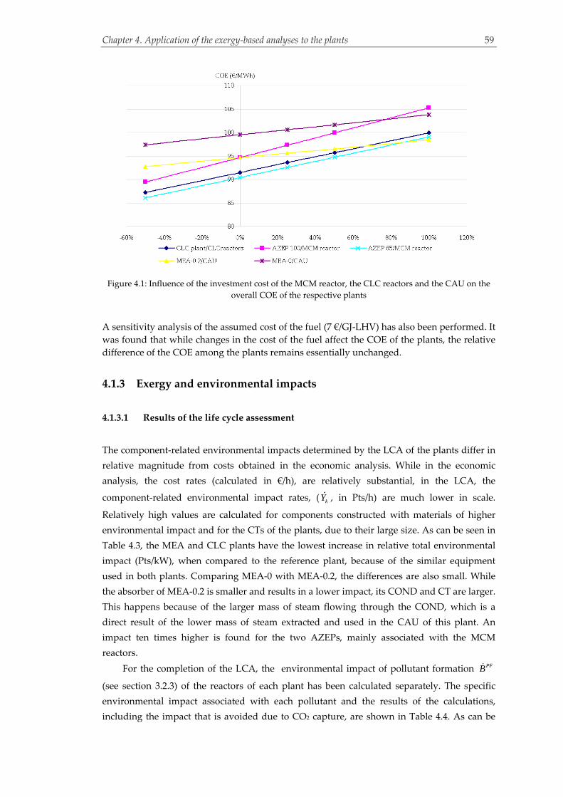
Chapter 4. Application of the exergy‐based analyses to the plants 59
Figure 4.1: Influence of the investment cost of the MCM reactor, the CLC reactors and the CAU on the
overall COE of the respective plants
A sensitivity analysis of the assumed cost of the fuel (7 €/GJ‐LHV) has also been performed. It
was found that while changes in the cost of the fuel affect the COE of the plants, the relative
difference of the COE among the plants remains essentially unchanged.
4.1.3 Exergy and environmental impacts
4.1.3.1 Results of the life cycle assessment
The component‐related environmental impacts determined by the LCA of the plants differ in
relative magnitude from costs obtained in the economic analysis. While in the economic
analysis, the cost rates (calculated in €/h), are relatively substantial, in the LCA, the
component‐related environmental impact rates, ( kY , in Pts/h) are much lower in scale.
Relatively high values are calculated for components constructed with materials of higher
environmental impact and for the CTs of the plants, due to their large size. As can be seen in
Table 4.3, the MEA and CLC plants have the lowest increase in relative total environmental
impact (Pts/kW), when compared to the reference plant, because of the similar equipment
used in both plants. Comparing MEA‐0 with MEA‐0.2, the differences are also small. While
the absorber of MEA‐0.2 is smaller and results in a lower impact, its COND and CT are larger.
This happens because of the larger mass of steam flowing through the COND, which is a
direct result of the lower mass of steam extracted and used in the CAU of this plant. An
impact ten times higher is found for the two AZEPs, mainly associated with the MCM
reactors.
For the completion of the LCA, the environmental impact of pollutant formation PFB
(see section 3.2.3) of the reactors of each plant has been calculated separately. The specific
environmental impact associated with each pollutant and the results of the calculations,
including the impact that is avoided due to CO2 capture, are shown in Table 4.4. As can be

Chapter 4. Application of the exergy‐based analyses to the plants 60
seen, 60% of pollutant formation in the reference plant is related to the CO2 emissions of the
plant, while the remaining 40% is related to its NOX emissions. The same NOX emissions are
considered for the MEA plants, while no NOX emissions are considered for the oxy‐fuel
plants. In the DB of the AZEP 85, combustion takes place with air, but the NOX emissions are
low due to the lower amount of reacting methane. The environmental impact of pollutants,
like CO2, can affect the result of the overall analysis. A sensitivity analysis of the impact of
CO2 emissions for the reference and MEA‐0.2 plant (with and without consideration of the
environmental impact of CO2 sequestration, Figures 4.2 and 4.3) has been performed in the
exergoenvironmental analysis.
Table 4.3: Selected results of the LCA
Ref.
Plant AZEP 85 AZEP 100 CLC MEA 0.2 MEA 0.0
Total environmental impact (103 Pts) 2,592 26,066 26,061 3,414 3,223 2,871
Total environmental impact (Pts/kW) 6.3 66.9 69.0 9.1 9.1 8.6
Table 4.4: Environmental impact of overall and avoided pollutant formation due to CO2 capture
CO2 NOX CH4 PFB 2 _
PFCO captB
(kg/s) (Pts/t) (kg/s) (Pts/t) (kg/s) (Pts/t) (Pts/h) (Pts/h)
Ref. Plant 38.41 0.05 1259 0
AZEP 85
DB
5.76 0.03 459 0
CC 32.65 641 ‐641
AZEP 100 38.42 754 ‐754
CLC plant 37.73 0.28 856 ‐741
MEA 0.2 38.42 0.05 1270 ‐646
MEA 0.0 38.42
5.4
0.05
2749.4
114.6
1268 ‐646
4.1.3.2 Results of the exergoenvironmental analysis
As shown in Table 4.5, the component‐related impact ( totY ) differs among the plants.
However, this difference is almost negligible and differences among the total impact
( , D tot totB Y ) of the reference and oxy‐fuel plants are determined by the impact of exergy
destruction. This indicates that the construction phase is not the key area for reducing the
environmental impact of these plants.
In the reference plant, the highest environmental impact ( , D k kB Y ) corresponds to the
CC, GT1, the LPST and C1. In the oxy‐fuel plants, the highest impact is caused by the
reactors, GT1, the FG COND and C1. In the AZEPs, the MCM LTHX also has a high impact.
In the MEA plant, the CC is followed by the CAU, which presents a high environmental
impact of exergy destruction. In the exergoenvironmental analysis, dissipative components
become more important than in the exergoeconomic analysis: a high impact is calculated for

Chapter 4. Application of the exergy‐based analyses to the plants 61
the condensers (COND and FG COND) of all of the plants. As already mentioned, in the
exergoeconomic and exergoenvironmental analyses, the influence of the non‐exergy related
costs/impacts (investment cost rate and rate of the component‐related impact) is different.
Because in the exergoenvironmental analysis the component‐related environmental impact is
almost negligible, the exergy destruction and the specific environmental impact of fuel are the
main deciding factors of the significance of a component. Differences between the results
of the exergoenvironmental analysis and that of the exergetic analysis are found for the
components constituting the MCM reactors. Here, the total environmental impact results in
relatively high values, leading to conclusions that diverge from those obtained by the
exergetic analysis.
The total exergoenvironmental factor is similar for plants with similar component‐
related environmental impact: approximately 4% for the AZEPs and around 0.5% for the
reference, CLC and MEA plants. A reduction in the overall environmental impact could be
achieved by increasing the exergetic efficiency of the GT system and the reactors. In general, a
decrease in the irreversibilities present in reactors is difficult because they are mostly
unavoidable. However, preheating of the reactants, as well as the use of different GT systems
(e.g., steam‐cooled expanders) would lead to better efficiencies, thus decreasing the incurred
exergy destruction. In the case of the oxy‐fuel plants, a further reduction of the overall
environmental impact could be achieved by decreasing the component‐related impact of the
reactors (e.g., by replacing the construction materials assumed, with materials of lower
impact), or by increasing the exergetic efficiency of the remaining components. In general, in
order to reduce the overall impact of the plants, more attention should be given to the
effectiveness of the component operation, thus the exergetic efficiencies of the components.
To compare the overall performance of the plants, the environmental impact of electricity
(EIE) has been calculated, the results of which are presented in Table 4.5. The environmental
impact of the electricity produced by the reference plant is found to be 25.1 Pts/MWh. This is
comparable to the European average impact of low voltage electricity: 26 Pts/MWh (SimaPro
7.1 manual, 2000). When compared to the reference plant, the EIE of the oxy‐fuel plants
presents a relatively low reduction, while that of MEA‐0.2 is increased by 2.3 Pts/MWh.
Considering that no impact has been considered for pollutants generated by the processing of
the solvent used in the plant, the case presented is considered the best case scenario of this
plant.
4.1.3.3 Sensitivity analyses
The high environmental impact of the MEA plant can have two possible interpretations: (1)
either the CO2 capture technology has no environmental benefit, but a penalty due to the high
decrease of the efficiency of the plant, or (2) the provided values of the environmental impact
of pollutants/reactants are not trustworthy. To examine the latter, a sensitivity analysis of the
environmental impacts of the CO2 emissions has been investigated. MEA‐0.2 has been further
considered for the sensitivity analysis, because it represents the most realistic alternative
between the two MEA plants and because it has the highest impact when compared to the
oxy‐fuel alternatives. The environmental impact of CO2 emissions (used for the calculation of

Chapter 4. Application of the exergy‐based analyses to the plants 62
pollutant formation) has been varied from ‐90% to +500% and the EIE has been calculated
with and without the addition of impact associated with mineral storage of the CO2 captured
(Khoo and Tan, 2006). The influence of these variations on the EIE of the MEA and the
reference plants is presented in Figures 4.2 and 4.3. As shown, CO2 capture becomes
meaningful when the environmental impact of CO2 is higher than 20 Pts/t (when storage is
also accounted for). This is a value approximately four times higher than that provided by
Goedkoop and Spriensma (2000), shown by the grey, dotted line. As shown in Figure 4.3,
when CO2 transport and sequestration are not accounted for, the limit for a positive
environmental impact of CO2 capture decreases to 14 Pts/t.
EIE (Pts/MWh)
20
25
30
35
0.0 5.0 10.0 15.0 20.0 25.0 30.0Impact of CO2 (Pts/t)
EIE‐MEA‐0.2/EI_CO2 EIE‐Ref. plant/EI_CO2
Figure 4.2: Influence of the specific environmental impact of CO2 on the EIE of the reference and MEA‐
0.2 plants, with consideration of an environmental impact of 4.9 Pts/t of CO2 associated with mineral
storage (the grey, dotted line shows the chosen, base value of the impact of CO2 emissions)
EIE (Pts/MWh)
20
25
30
35
0.0 5.0 10.0 15.0 20.0 25.0 30.0Impact of CO2 (Pts/t)
EIE‐MEA‐0.2/EI_CO2 EIE‐Ref. plant/EI_CO2
Figure 4.3: Influence of the specific environmental impact of CO2 on the EIE of the reference and MEA‐
0.2 plants without consideration of the environmental impact associated with CO2 mineral storage (the
grey, dotted line shows the chosen, base value of the impact of CO2 emissions)

Chapter 4. Application of the exergy‐based analyses to the plants 63
Table 4.5: Results of the conventional exergy‐based analyses for the overall plants
Ref. Plant AZEP 85 AZEP 100 CLC Plant MEA 0.2 S‐GRAZ ATR Plant MEA 0.0 MSR Plant Simple oxy‐fuel Plant
CO2 emitted (kg/s) 38.72 6.06 0.35 0.35 5.81 0.00 9.62 5.81 0.26 0.13
CO2 emitted (kg/MWh) 337.90 55.97 3.36 3.39 59.10 0.00 101.87 62.49 2.80 1.54
CO2 captured (kg/s) ‐ 32.71 38.48 37.73 32.91 38.58 29.08 32.91 37.95 38.58
CO2 captured (%) ‐ 84.4 99.1 99.1 85.0 100.0 75.2 85.0 99.3 99.7
Total FCI (106€) 213 395 414 362 326 319
Total FCI (€/kW) 517 1012 1097 962 921 953
Total FCI (106€/kg CO2 capt.) ‐ 12.1 10.8 9.6 9.9 9.7
Total environmental impact (Pts) 2,592 26,066 26,061 3,414 3,223 2,871
Total environmental impact (Pts/kW) 6.3 66.9 69.0 9.1 9.1 8.6
COE (€/MWh) 74.1 90.4 94.7 91.4 94.6 99.5
COA‐CO2 (€/t) N/A 57.8 61.6 52.0 73.5 92.2
EIE (Pts/MWh) 25.1 24.9 24.5 24.5 27.4 29.0
COA‐CO2: Cost of avoided CO2, COE: Cost of electricity, EI: Environmental impact, EIE: Environmental impact of electricity, FCI: Fixed capital investment
Table 4.6: Selected results at the component level for the reference plant
,F kE ,P kE ,D kE k ,D ky ,F kc ,P kc ,D kC kZ ,D k kC Z kf kr ,F kb ,P kb
,D kB kY ,D k kB Y ,b kf ,b kr
Component, k (MW) (MW) (MW) (%) (%) (€/GJ) (€/GJ) (€/h) (€/h) (€/h) (%) (%) (Pts/GJ) (Pts/GJ) (Pts/h) (Pts/h) (Pts/h) (%) (%)
C1 242.68 231.30 11.38 95.3 1.56 16.9 19.5 693 1,423 2,116 67.3 15.0 6.1 6.4 249.71 0.24 249.94 0.09 4.9CC 729.62 508.76 220.87 69.7 30.23 9.2 13.7 7,276 1,017 8,293 12.3 49.5 3.5 5.6 2746.20 0.38 2746.58 0.01 63.3GT 551.15 530.67 20.47 96.3 2.80 15.5 16.9 1,140 1,627 2,766 58.8 9.4 5.9 6.1 432.58 1.12 433.71 0.26 3.9HPSH 35.07 31.72 3.35 90.5 15.5 19.4 25.6 5.9 6.8 15.5HPEV 43.64 39.91 3.73 91.5 15.5 19.0 23.1 5.9 6.7 13.6HPEC 28.92 24.91 4.00 86.2 1.52 15.5 20.4 617 432 1,049 41.2 31.8 5.9 7.2 234.07 1.42 235.49 0.60 23.3RH 26.47 23.89 2.58 90.3 15.5 19.4 25.4 5.9 6.8 15.8IPSH 0.18 0.12 0.06 69.0 15.5 35.4 128.8 5.9 9.7 65.2IPEV 6.10 5.67 0.43 92.9 15.5 20.5 32.8 5.9 6.5 11.1IPEC 1.06 0.87 0.19 82.5 0.44 15.5 22.3 181 186 367 50.7 44.3 5.9 7.7 68.64 0.85 69.49 1.22 30.9LPSH 1.43 1.04 0.38 73.3 15.5 29.5 90.9 5.9 9.0 53.0LPEV 19.03 15.48 3.55 81.4 15.5 24.2 56.4 5.9 7.8 33.3LPEC 11.49 7.71 3.78 67.1 1.06 15.5 30.8 429 287 716 40.1 99.3 5.9 10.1 162.97 0.23 163.20 0.14 71.3LPST 70.99 61.35 9.64 86.4 1.32 21.4 29.7 743 764 1,508 50.7 38.5 7.2 8.8 251.49 0.49 251.98 0.20 21.5Total 730.58 412.54 300.41 56.5 41.12 9.2 20.6 9,897 6,519 16,416 39.7 124.8 3.5 7.0 3735.22 17.33 3752.54 0.46 101.7Exergy loss 17.63
PFkB (Pts/h) 1259
Chapter 4. A
pplication of the exergy‐based an
alyses to the plants
63

Chapter 4. Application of the exergy‐based analyses to the plants 64
Table 4.7: Selected results at the component level for the AZEP 85
,F kE ,P kE ,D kE k ,D ky ,F kc ,P kc ,D kC kZ ,D k kC Z kf kr ,F kb ,P kb ,D kB kY ,D k kB Y
,b kf ,b kr
Component, k (MW) (MW) (MW) (%) (%) (€/GJ) (€/GJ) (€/h) (€/h) (€/h) (%) (%) (Pts/GJ) (Pts/GJ) (Pts/h) (Pts/h) (Pts/h) (%) (%)
C1 238.30 227.13 11.17 95.3 1.53 19.8 22.2 797 1,169 1,966 59.5 12.1 6.2 6.5 250.79 0.19 250.98 0.08 4.9
CC 620.26 466.61 153.65 75.2 21.03 9.3 12.7 5,120 746 5,866 12.7 37.7 3.5 5.0 1932.51 0.31 1932.82 0.02 43.9
MCM 82.65 77.03 5.62 93.2 0.77 13.6 18.9 275 1,192 1,468 81.2 38.9 5.1 8.9 103.16 53.34 156.50 34.08 75.2
MCM HTHX 120.72 119.49 1.24 99.0 0.17 13.6 15.4 61 696 757 92.0 12.9 5.1 5.2 22.79 32.67 55.46 58.90 2.5
MCM LTHX 221.06 211.51 9.55 95.7 1.31 13.6 15.7 467 1,113 1,580 70.4 15.3 5.1 5.4 175.99 67.57 243.56 27.74 6.2
DB 109.46 78.20 31.26 71.4 4.28 9.3 13.9 1,042 277 1,318 21.0 50.6 3.5 6.5 393.12 0.05 393.17 0.01 86.6
GT1 495.66 477.85 17.81 96.4 2.44 18.4 19.8 1,177 1,336 2,513 53.2 8.0 6.0 6.2 385.39 0.91 386.30 0.23 3.7
C6 7.31 7.07 0.24 96.8 0.03 36.4 61.5 31 607 638 95.1 68.9 10.0 10.4 8.54 0.60 9.14 6.53 3.6
AIR HX 6.91 5.15 1.76 74.5 0.24 13.1 18.0 83 8 91 8.8 37.5 5.1 6.8 32.09 0.00 32.09 0.01 34.2
NGPH 5.80 0.10 5.70 1.7 0.78 13.1 795.8 269 6 275 2.2 5974.4 5.1 301.0 103.97 0.00 103.97 0.00 5843.8
HPSH 31.65 28.65 3.00 90.5 18.4 22.6 23.1 6.0 6.9 14.9
HPEV 39.82 36.29 3.54 91.1 18.4 22.2 21.2 6.0 6.8 13.8
HPEC 26.17 22.65 3.52 86.6 1.38 18.4 23.6 664 383 1,047 36.6 28.6 6.0 7.3 217.49 1.29 218.78 0.59 21.9
LPSH 1.06 0.77 0.29 72.5 18.4 34.2 86.3 6.0 9.2 53.6
LPEV 15.25 12.50 2.75 81.9 18.4 27.6 50.4 6.0 7.9 31.1
LPEC 11.20 7.83 3.37 69.9 0.88 18.4 33.8 424 262 686 38.3 83.9 6.0 9.7 138.76 0.22 138.98 0.16 60.7
LPST 49.32 42.62 6.70 86.4 0.92 24.4 32.8 587 489 1,077 45.4 34.6 7.3 8.8 175.98 0.37 176.35 0.21 21.1
ST4 27.92 21.14 6.78 75.7 0.93 22.8 36.4 557 257 814 31.5 59.6 7.0 10.0 170.64 0.22 170.86 0.13 43.5
C2 3.38 2.81 0.57 83.3 36.4 169.1 364.3 10.0 39.8 297.3
C3 3.48 2.88 0.60 82.8 36.4 86.6 137.9 10.0 13.7 36.2
C4 3.47 2.85 0.62 82.2 36.4 91.2 150.5 10.0 14.3 42.9
C5 3.52 2.85 0.66 81.2 0.33 36.4 93.2 320 1,425 1,745 81.7 156.0 10.0 14.5 88.15 0.23 88.37 0.26 45.1
Total 730.56 389.89 313.43 53.4 42.90 9.2 25.1 10,326 11,198 21,524 52.0 174.3 3.5 6.9 3897.09 174.95 4072.05 4.30 100.2
Exergy loss 27.25
PFB (Pts/h) 641 (CC)
459 (DB)
Chapter 4. A
pplication of the exergy‐based an
alyses to the plants
64

Chapter 4. Application of the exergy‐based analyses to the plants 65
Table 4.8: Selected results at the component level for the AZEP 100
,F kE ,P kE ,D kE k ,D ky ,F kc ,P kc ,D kC kZ ,D k kC Z kf kr ,F kb ,P kb ,D kB kY ,D k kB Y ,b kf ,b kr
Component, k (MW) (MW) (MW) (%) (%) (€/GJ) (€/GJ) (€/h) (€/h) (€/h) (%) (%) (Pts/GJ) (Pts/GJ) (Pts/h) (Pts/h) (Pts/h) (%) (%)
C1 280.47 267.32 13.15 95.3 1.80 20.6 22.8 975 1,133 2,108 53.8 10.6 6.1 6.4 288.47 0.18 288.65 0.06 4.9
CC 729.72 549.07 180.65 75.2 24.72 9.3 12.7 6,020 831 6,851 12.1 37.4 3.5 5.0 2272.15 0.30 2272.44 0.01 43.8
MCM 97.30 90.54 6.75 93.1 0.92 13.6 19.1 330 1,459 1,789 81.6 40.4 5.1 8.4 123.85 35.87 159.72 22.46 65.9
MCM HTHX 142.04 140.61 1.43 99.0 0.20 13.6 15.3 70 791 861 91.9 12.5 5.1 5.2 26.38 38.37 64.75 59.25 2.5
MCM LTHX 260.08 248.86 11.22 95.7 1.54 13.6 15.6 548 1,270 1,818 69.8 15.0 5.1 5.4 206.67 79.33 286.01 27.74 6.2
GT1 532.11 512.51 19.60 96.3 2.68 19.2 20.6 1,352 1,295 2,647 48.9 7.5 5.9 6.1 414.12 0.87 415.00 0.21 3.8
C6 8.59 8.31 0.28 96.8 0.04 37.7 61.5 38 675 713 94.7 63.1 9.9 10.2 9.85 0.60 10.44 5.71 3.5
AIR HX 8.20 6.12 2.09 74.6 0.29 13.1 18.0 98 9 107 8.6 37.3 5.1 6.8 38.02 0.00 38.02 0.01 34.1
NGPH 5.82 0.10 5.72 1.7 0.78 13.1 791.7 269 6 275 2.2 5955.1 5.1 300.1 104.32 0.00 104.32 0.00 5826.8
HPSH 18.82 17.15 1.68 91.1 19.2 23.8 24.2 5.9 6.7 14.1
HPEV 32.96 30.50 2.46 92.5 19.2 23.0 19.9 5.9 6.5 11.5
HPEC 22.53 19.04 3.49 84.5 1.04 19.2 25.3 526 340 866 39.3 32.2 5.9 7.4 161.13 1.03 162.16 0.63 26.1
LPSH 1.08 0.78 0.31 71.8 19.2 36.2 88.7 5.9 9.2 56.0
LPEV 16.73 13.76 2.97 82.2 19.2 28.6 49.5 5.9 7.7 30.8
LPEC 12.06 8.19 3.87 67.9 0.98 19.2 36.1 494 277 771 36.0 88.5 5.9 9.8 151.16 0.23 151.39 0.15 67.4
LPST 44.78 38.70 6.08 86.4 0.83 25.8 34.5 564 435 999 43.5 33.7 7.2 8.8 158.54 0.34 158.88 0.21 21.1
ST4 32.85 24.83 8.02 75.6 1.10 23.7 37.7 686 288 974 29.6 58.9 6.9 9.9 198.25 0.24 198.49 0.12 44.0
C2 3.96 3.31 0.66 83.4 37.7 167.7 344.5 9.9 39.4 298.4
C3 4.08 3.39 0.69 83.0 37.7 86.1 128.3 9.9 13.5 36.1
C4 4.07 3.35 0.72 82.2 37.7 90.7 140.4 9.9 14.1 42.9
C5 4.13 3.36 0.78 81.2 0.39 37.7 92.8 387 1,583 1,970 80.3 145.8 9.9 14.3 101.52 0.23 101.75 0.22 45.0
Total 730.73 377.52 320.71 51.7 43.89 9.2 26.3 10,566 11,706 22,272 52.6 187.4 3.5 6.8 3987.65 174.91 4162.56 4.20 97.0
Exergy loss 32.50 PFkB (Pts/h) 754
Chapter 4. A
pplication of the exergy‐based an
alyses to the plants
65

Chapter 4. Application of the exergy‐based analyses to the plants 66
Table 4.9: Selected results at the component level for the CLC plant
,F kE ,P kE ,D kE k ,D ky ,F kc ,P kc ,D kC kZ ,D k kC Z kf kr ,F kb ,P kb ,D kB kY ,D k kB Y ,b kf ,b kr
Component, k (MW) (MW) (MW) (%) (%) (€/GJ) (€/GJ) (€/h) (€/h) (€/h) (%) (%) (Pts/GJ) (Pts/GJ) (Pts/h) (Pts/h) (Pts/h) (%) (%)
C1 281.78 268.57 13.21 95.3 1.81 19.3 21.3 919 964 1,884 51.2 10.1 6.0 6.3 286.48 0.19 286.67 0.07 4.9
CLC 694.73 500.67 194.06 72.1 26.56 9.1 15.5 6,391 4,974 11,365 43.8 68.9 3.5 5.3 2418.44 2.54 2420.97 0.10 52.5
GT1 540.99 521.34 19.65 96.4 2.69 18.1 19.3 1,278 1,102 2,380 46.3 7.0 5.8 6.0 410.68 0.91 411.59 0.22 3.8
NGPH 6.32 1.12 5.20 17.7 0.71 11.8 69.1 220 10 231 4.4 487.2 4.1 22.9 75.87 0.01 75.88 0.01 465.6
HPSH 22.43 20.43 1.99 91.1 18.1 22.2 22.7 5.8 7.1 14.3
HPEV 35.74 32.97 2.77 92.2 18.1 21.5 19.2 5.8 6.6 12.1
HPEC 24.25 20.58 3.67 84.9 1.15 18.1 23.7 548 301 850 35.5 31.2 5.8 6.5 176.20 1.16 177.36 0.65 25.6
RH 16.60 14.36 2.24 86.5 18.1 23.4 29.4 5.8 7.3 22.6
IPSH 0.63 0.49 0.14 78.1 18.1 30.2 67.0 5.8 8.2 40.5
IPEV 11.97 11.00 0.97 91.9 18.1 22.8 26.1 5.8 6.5 12.8
IPEC 2.03 1.70 0.33 83.6 0.50 18.1 24.8 240 161 400 40.1 37.4 5.8 7.4 77.03 0.53 77.56 0.69 28.2
LPSH 1.12 0.81 0.32 71.9 18.1 33.4 84.8 5.8 9.1 56.2
LPEV 17.03 13.99 3.03 82.2 18.1 26.7 47.7 5.8 7.6 31.2
LPEC 11.28 7.52 3.76 66.6 0.97 18.1 34.4 463 221 684 32.4 90.7 5.8 10.0 148.65 0.22 148.87 0.15 72.1
LPST 48.80 42.17 6.63 86.4 0.91 24.6 32.5 587 387 974 39.7 32.0 7.2 8.8 172.69 0.36 173.05 0.21 21.3
ST4 20.73 15.66 5.06 75.6 0.69 23.2 36.5 424 157 580 27.0 57.2 6.9 10.0 125.88 0.18 126.07 0.15 44.3
C1 3.85 3.24 0.61 84.1 36.5 165.8 353.6 10.0 40.4 305.3
C2 3.96 3.32 0.64 83.8 36.5 76.3 108.9 10.0 13.1 31.0
C3 3.91 3.27 0.64 83.5 36.5 78.8 115.8 10.0 13.5 35.5
C4 3.93 3.26 0.67 83.0 0.35 36.5 79.8 338 1,275 1,612 79.1 118.5 10.0 13.6 92.03 0.23 92.26 0.25 36.6
Total 730.73 375.99 307.41 51.5 42.07 9.2 25.4 10,128 10,347 20,474 50.5 177.5 3.5 6.8 3822.32 22.84 3845.17 0.59 94.5
Exergy loss 47.33 PFkB (Pts/h) 856
Chapter 4. A
pplication of the exergy‐based an
alyses to the plants
66
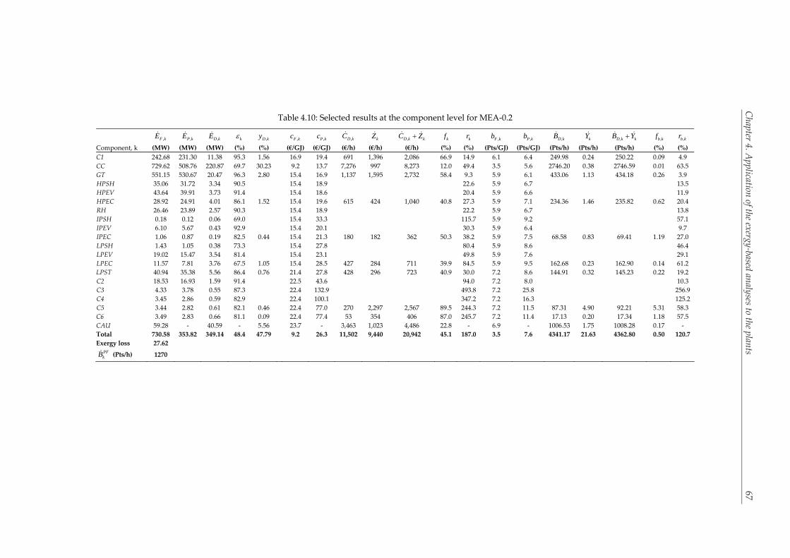
Chapter 4. Application of the exergy‐based analyses to the plants 67
Table 4.10: Selected results at the component level for MEA‐0.2
,F kE ,P kE ,D kE k ,D ky ,F kc ,P kc ,D kC kZ ,D k kC Z kf kr ,F kb ,P kb ,D kB kY ,D k kB Y ,b kf ,b kr
Component, k (MW) (MW) (MW) (%) (%) (€/GJ) (€/GJ) (€/h) (€/h) (€/h) (%) (%) (Pts/GJ) (Pts/GJ) (Pts/h) (Pts/h) (Pts/h) (%) (%)
C1 242.68 231.30 11.38 95.3 1.56 16.9 19.4 691 1,396 2,086 66.9 14.9 6.1 6.4 249.98 0.24 250.22 0.09 4.9
CC 729.62 508.76 220.87 69.7 30.23 9.2 13.7 7,276 997 8,273 12.0 49.4 3.5 5.6 2746.20 0.38 2746.59 0.01 63.5
GT 551.15 530.67 20.47 96.3 2.80 15.4 16.9 1,137 1,595 2,732 58.4 9.3 5.9 6.1 433.06 1.13 434.18 0.26 3.9
HPSH 35.06 31.72 3.34 90.5 15.4 18.9 22.6 5.9 6.7 13.5
HPEV 43.64 39.91 3.73 91.4 15.4 18.6 20.4 5.9 6.6 11.9
HPEC 28.92 24.91 4.01 86.1 1.52 15.4 19.6 615 424 1,040 40.8 27.3 5.9 7.1 234.36 1.46 235.82 0.62 20.4
RH 26.46 23.89 2.57 90.3 15.4 18.9 22.2 5.9 6.7 13.8
IPSH 0.18 0.12 0.06 69.0 15.4 33.3 115.7 5.9 9.2 57.1
IPEV 6.10 5.67 0.43 92.9 15.4 20.1 30.3 5.9 6.4 9.7
IPEC 1.06 0.87 0.19 82.5 0.44 15.4 21.3 180 182 362 50.3 38.2 5.9 7.5 68.58 0.83 69.41 1.19 27.0
LPSH 1.43 1.05 0.38 73.3 15.4 27.8 80.4 5.9 8.6 46.4
LPEV 19.02 15.47 3.54 81.4 15.4 23.1 49.8 5.9 7.6 29.1
LPEC 11.57 7.81 3.76 67.5 1.05 15.4 28.5 427 284 711 39.9 84.5 5.9 9.5 162.68 0.23 162.90 0.14 61.2
LPST 40.94 35.38 5.56 86.4 0.76 21.4 27.8 428 296 723 40.9 30.0 7.2 8.6 144.91 0.32 145.23 0.22 19.2
C2 18.53 16.93 1.59 91.4 22.5 43.6 94.0 7.2 8.0 10.3
C3 4.33 3.78 0.55 87.3 22.4 132.9 493.8 7.2 25.8 256.9
C4 3.45 2.86 0.59 82.9 22.4 100.1 347.2 7.2 16.3 125.2
C5 3.44 2.82 0.61 82.1 0.46 22.4 77.0 270 2,297 2,567 89.5 244.3 7.2 11.5 87.31 4.90 92.21 5.31 58.3
C6 3.49 2.83 0.66 81.1 0.09 22.4 77.4 53 354 406 87.0 245.7 7.2 11.4 17.13 0.20 17.34 1.18 57.5
CAU 59.28 ‐ 40.59 ‐ 5.56 23.7 ‐ 3,463 1,023 4,486 22.8 ‐ 6.9 ‐ 1006.53 1.75 1008.28 0.17 ‐
Total 730.58 353.82 349.14 48.4 47.79 9.2 26.3 11,502 9,440 20,942 45.1 187.0 3.5 7.6 4341.17 21.63 4362.80 0.50 120.7
Exergy loss 27.62 PFkB (Pts/h) 1270
Chapter 4. A
pplication of the exergy‐based an
alyses to the plants
67
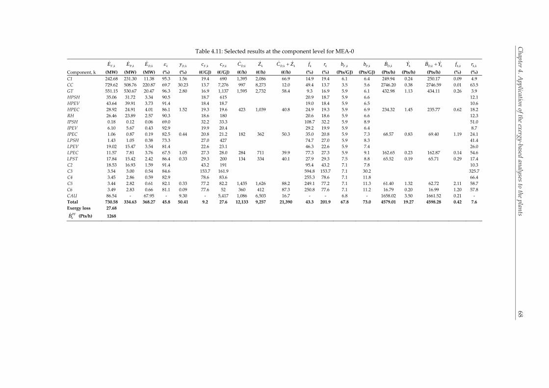
Chapter 4. Application of the exergy‐based analyses to the plants 68
Table 4.11: Selected results at the component level for MEA‐0
,F kE ,P kE ,D kE k ,D ky ,F kc ,P kc ,D kC kZ ,D k kC Z kf kr ,F kb ,P kb ,D kB kY ,D k kB Y ,b kf ,b kr
Component, k (MW) (MW) (MW) (%) (%) (€/GJ) (€/GJ) (€/h) (€/h) (€/h) (%) (%) (Pts/GJ) (Pts/GJ) (Pts/h) (Pts/h) (Pts/h) (%) (%)
C1 242.68 231.30 11.38 95.3 1.56 19.4 690 1,395 2,086 66.9 14.9 19.4 6.1 6.4 249.94 0.24 250.17 0.09 4.9
CC 729.62 508.76 220.87 69.7 30.23 13.7 7,276 997 8,273 12.0 49.4 13.7 3.5 5.6 2746.20 0.38 2746.59 0.01 63.5
GT 551.15 530.67 20.47 96.3 2.80 16.9 1,137 1,595 2,732 58.4 9.3 16.9 5.9 6.1 432.98 1.13 434.11 0.26 3.9
HPSH 35.06 31.72 3.34 90.5 18.7 615 18.7 5.9 6.6 12.1
HPEV 43.64 39.91 3.73 91.4 18.4 18.7 18.4 5.9 6.5 10.6
HPEC 28.92 24.91 4.01 86.1 1.52 19.3 19.6 423 1,039 40.8
20.9
19.0
24.9 19.3 5.9 6.9 234.32 1.45 235.77 0.62 18.2
RH 26.46 23.89 2.57 90.3 18.6 180 18.6 5.9 6.6 12.3
IPSH 0.18 0.12 0.06 69.0 32.2 33.3 32.2 5.9 8.9 51.0
IPEV 6.10 5.67 0.43 92.9 19.9 20.4 19.9 5.9 6.4 8.7
IPEC 1.06 0.87 0.19 82.5 0.44 20.8 21.2 182 362 50.3
20.6
108.7
29.2
35.0 20.8 5.9 7.3 68.57 0.83 69.40 1.19 24.1
LPSH 1.43 1.05 0.38 73.3 27.0 427 27.0 5.9 8.3 41.4
LPEV 19.02 15.47 3.54 81.4 22.6 23.1 22.6 5.9 7.4 26.0
LPEC 11.57 7.81 3.76 67.5 1.05 27.3 28.0 284 711 39.9
74.7
46.3
77.3 27.3 5.9 9.1 162.65 0.23 162.87 0.14 54.6
LPST 17.84 15.42 2.42 86.4 0.33 29.3 200 134 334 40.1 27.9 29.3 7.5 8.8 65.52 0.19 65.71 0.29 17.4
C2 18.53 16.93 1.59 91.4 43.2 191 43.2 7.1 7.8 10.3
C3 3.54 3.00 0.54 84.6 153.7 161.9 153.7 7.1 30.2 325.7
C4 3.45 2.86 0.59 82.9 78.6 83.6 78.6 7.1 11.8 66.4
C5 3.44 2.82 0.61 82.1 0.33 77.2 82.2 1,435 1,626 88.2
95.4
594.8
255.3
249.1 77.2 7.1 11.3 61.40 1.32 62.72 2.11 58.7
C6 3.49 2.83 0.66 81.1 0.09 77.6 52 360 412 87.3 250.8 77.6 7.1 11.2 16.79 0.20 16.99 1.20 57.8
CAU 86.54 ‐ 67.95 ‐ 9.30 ‐ 5,417 1,086 6,503 16.7 ‐ ‐ 6.8 ‐ 1658.02 3.50 1661.52 0.21 ‐
Total 730.58 334.63 368.27 45.8 50.41 9.2 27.6 12,133 9,257 21,390 43.3 201.9 67.8 73.0 4579.01 19.27 4598.28 0.42 7.6
Exergy loss 27.68 PFkB (Pts/h) 1268
Chapter 4. A
pplication of the exergy‐based an
alyses to the plants
68

Chapter 4. Application of the exergy‐based analyses to the plants 69
Table 4.12: Selected results at the component level for the S‐Graz cycle and the simple oxy‐fuel plant
S‐Graz cycle ATR plant
,F kE ,P kE ,D kE k ,D ky ,F kE ,P kE ,D kE k ,D ky
Component, k (MW) (MW) (MW) (%) (%) Component, k (MW) (MW) (MW) (%) (%)
C1 53.76 50.84 2.92 94.6 0.40 C1 56.60 53.53 3.07 94.6 0.42
CC 736.37 551.82 184.55 74.9 25.17 CC 733.81 512.57 221.24 69.9 30.18
GT1 264.57 253.32 11.25 95.7 1.53 GT 437.91 420.80 17.11 96.1 2.33
GT2 362.41 345.23 17.18 95.3 2.34 HPSH 41.65 35.88 5.78 86.1 2.44
GT3 78.21 69.56 8.65 88.9 1.18 HPEV 51.98 45.21 6.78 87.0
HPSH 52.48 46.00 6.48 87.7 HPEC 33.59 28.22 5.37 84.0
HPEV 65.48 58.00 7.47 88.6 RH 22.83 18.78 4.05 82.3 0.61
HPEC 1.35 1.27 0.08 93.9
1.91
IPSH 0.10 0.06 0.04 61.4
NGPH 7.05 3.61 3.44 51.2 0.47 IPEV 4.45 4.20 0.25 94.4
WPH1 5.57 3.09 2.48 55.5 IPEC 0.77 0.65 0.13 83.7
WPH2 31.83 25.56 6.27 80.3 LPSH 0.85 0.62 0.23 72.9 0.67
WPH3 16.19 14.67 1.52 90.6
1.40
LPEV 12.43 10.24 2.20 82.3
ASU 51.24 11.46 39.78 22.4 5.43 LPEC 10.23 7.73 2.50 75.6
C2 12.45 11.04 1.41 88.7 LPST 51.25 44.29 6.96 86.4 0.95
C3 4.69 3.95 0.74 84.1 ST4 21.91 19.22 2.69 87.7 0.37
C4 4.70 3.93 0.77 83.5 ASU 53.95 11.59 42.36 21.5 5.78
C5 4.75 3.94 0.81 83.0
0.51
C2 4.82 4.05 0.78 83.9 0.44
C7 92.86 86.56 6.30 93.2 C3 4.80 4.01 0.79 83.5
C8 132.31 124.67 7.63 94.2 1.90
C4 4.76 3.95 0.81 83.0
C9 16.43 13.73 2.70 83.5 C5 4.83 3.96 0.87 82.1
C10 17.72 14.93 2.80 84.2 0.75
C6 62.77 57.08 5.70 90.9 1.03
Total 733.16 352.01 349.26 48.0 47.64 C7 56.67 54.82 1.85 96.7
Exergy loss 31.89 C8 16.43 13.73 2.70 83.5 0.75
C9 17.89 15.08 2.81 84.3
Total 733.18 313.40 388.71 42.7 53.02
Exergy loss 31.08
Table 4.13: Selected results at the component level for the MSR and ATR plants
MSR plant ATR plant
,F kE ,P kE ,D kE k ,D ky ,F kE ,P kE ,D kE k ,D ky
Component, k (MW) (MW) (MW) (%) (%) Component, k (MW) (MW) (MW) (%) (%)
C1 206.31 196.73 9.58 95.4 1.31 C1 221.95 211.43 10.53 95.3 1.44
CC 598.70 455.59 143.11 76.1 19.59 CC 659.64 502.80 156.84 76.2 21.47
DB 338.16 252.94 85.23 74.8 11.66 GT1 519.91 500.85 19.06 96.3 2.61
GT1 481.89 463.51 18.37 96.2 2.51 HPSH1 2.37 2.06 0.31 86.9 1.14
GT2 54.18 50.81 3.37 93.8 0.46 HPSH2 26.00 23.38 2.62 89.9
HPSH 36.79 32.41 4.38 88.1 HPEV 36.90 32.76 4.14 88.8
HPEV 47.13 40.95 6.17 86.9 HPEC 10.69 9.40 1.29 87.9
HPEC 32.45 25.58 6.86 78.8
2.38
RH1 11.37 10.65 0.72 93.7 0.97
LPSH 3.17 2.40 0.77 75.7 RH2 8.76 7.95 0.81 90.8
LPEV 27.16 21.11 6.05 77.7 IPSH 5.51 4.72 0.79 85.6
LPEC 13.93 9.33 4.60 67.0
1.56
IPEV 30.37 26.75 3.62 88.1
NGPH 32.62 28.56 4.06 87.6 0.56 IPEC 6.89 5.75 1.14 83.5
LPST 22.33 19.29 3.03 86.4 0.42 LPSH1 1.54 1.14 0.40 74.1 1.25
MSR‐H2 180.20 171.88 8.32 95.4 1.14 LPSH2 3.37 2.86 0.52 84.7
C2 3.84 3.19 0.64 83.2 LPEV 19.39 15.73 3.66 81.1
C3 4.06 3.37 0.69 83.0 LPEC 13.01 8.44 4.57 64.9
C4 4.04 3.33 0.71 82.4 NGPH 34.36 30.19 4.17 87.9 0.57
C5 4.10 3.34 0.76 81.4
0.38
H2 PH 32.61 25.32 7.30 77.6 1.00
Total 730.63 334.64 338.70 45.8 46.36 APH 9.38 5.91 3.47 63.0 0.47
Exergy loss 57.29 LPST 23.85 20.61 3.24 86.4 0.44
ATR 809.32 ‐ 51.81 ‐ 7.09
SHIFTER1 690.54 ‐ 3.43 ‐ 0.47
SHIFTER2 659.61 ‐ 0.63 ‐
CAU 33.54 ‐ 29.95 ‐ 4.10
Mix CH4/Air 428.31 419.98 8.33 98.1 1.14
Mix CH4/H2O 507.54 500.94 6.60 98.7 0.90
Total 730.62 339.81 358.06 46.5 49.01
Exergy loss 32.75

Chapter 4. Application of the exergy‐based analyses to the plants 70
4.2 Advanced exergy‐based analyses
The advanced exergetic, exergoeconomic and exergoenvironmental analyses have been
applied to the reference plant and the two most economical plants performing CO2 capture,
the AZEP 85 and the CLC plant.
4.2.1 Advanced exergetic analysis
4.2.1.1 Application of the advanced exergetic analysis
To conduct the advanced exergetic analysis, the theoretical and unavoidable conditions for all
the components must be defined (see section 3.3). For the calculation of the unavoidable
exergy destruction, the best possible operating conditions are considered for each component.
These calculations regard each component in isolation, thus simultaneous component
interactions are not a concern here. On the other hand, the calculation of the endogenous
exergy destruction involves theoretical operation of components, considers the overall plant
and it, therefore, examines simultaneous component interactions (mexogenous exergy
destruction, Equation 3.21) as well. For the calculation of the endogenous exergy destruction
of component k, component k operates under real conditions, while all other components
operate theoretically. For the calculation of component interactions, the examined
components operate under real conditions in pairs, while all remaining components operate
theoretically. The assumptions made for the theoretical and unavoidable operation of all of
the components are shown in Table 4.14.
Assumptions related to the theoretical operation of components include zero pressure
losses, high efficiencies, low temperature differences, etc. When a component operates
without pressure losses, the pressure losses of any parallel components are also considered to
be zero, even if the parallel components operate under real conditions. Additionally, changes
in the minimum temperature differences of some components might affect the operation of
parallel components by increasing or decreasing their exergy destruction. As already
mentioned, in the description of the methodology (section 3.3.1), theoretical reactors are
defined using the exergy balance, while the mass and energy balances of the components are
not maintained. To achieve this, the plants are split into two parts after each reactor.
In the case of the reference plant, when either the CC or the neighboring components
operate theoretically, streams 3 and 4 Figure 4.44 will differ to maintain the predefined (either
real‐ or theoretical‐related) exergy balance of the reactor. When theoretical operation is
assumed for a component or a group of components, the mass flows of the required air and
fuel are calculated through the net power output of the plant, netW , and the excess air fraction
( ) of the CC, which have the same values as in the real case. For the calculation of the
endogenous exergy destruction, the CC must operate with its real exergetic efficiency
4 For simplicity, the numbering of the streams in Figure 4.4 differs from that in Figure A.1.1. The correlation of the
numbers in Figure 4.4 with Figure A.1.1 is the following: 1 is 1, 2 is 2, 3&4 are 4, 5 is 5 and 6 is 3.

Chapter 4. Application of the exergy‐based analyses to the plants 71
Table 4.14: Assumptions related to the theoretical and unavoidable operation of the components
Component,
k ,
realD kE Theoretical
operation ,
UND kE Component,
k ,
realD kE Theoretical
operation ,
UND kE
ηis =92‐94% ηis =100% ηis =96% ηis =75‐79% ηis =100% ηis =94% GT1
ηmech =99% ηmech =100% ηmech =100% C2‐C5
ηmech =99% ηmech =100% ηmech =100%
ηis =90‐94% ηis =100% ηis =96% ηis =96.8% ηis =100% ηis =94% GT2
ηmech =99% ηmech =100% ηmech =100% C6
ηis =85‐88% ηmech =100% ηmech =100%
ηis =91‐94% ηis =100% ηis =94% ΔTmin =20°C ΔTmin =0 ΔTmin =4 C1
ηmech =99% ηmech =100% ηmech =100% ΔPHSa ΔP =0 ΔP =0
Qloss =0.01 Qloss =0 Qloss =0
SH/RH
ΔPCS =5%f
ΔP =3%f ΔP =0 ΔP =0 Pinch point =10°C ΔTmin =0 ΔTmin =1 CC
λ=2.05 λ=2.05 λ=1 Appr. T =6°C Appr. T =0 Appr. T =0
Qloss =0.01 Qloss =0 Qloss =0 ΔPHSa ΔP =0 ΔP =0
ΔP =1%f ΔP =0 ΔP =0
EV
ΔPCS =5%b,f DB
λ=10 λ=10 d λ=1 ΔTmin=dependantg ΔTmin =0 ΔTmin =1
η =86‐94% ηis =100% ηis =95% HP,
IP 92% LP ΔPHS a ΔP =0 ΔP =0
STs
ηmech =99% ηmech =100% ηmech =100%
EC
ΔPCS =3%/100°C
Qloss =0 Qloss =0 Qloss =0 ΔTmin=400e ΔTmin=dependantg ΔTmin =20
ΔP =3%f ΔP =0 ΔP =0 ΔPHP=0.65%
bar/100°C ΔP =0 ΔP =0 CLC
Reactors
λ=1.05 λ=1.05 λ=1
NGPH
ΔPLP=0.60%
bar/100°C
Qloss =0.0 Qloss =0 Qloss =0 ΔTmin=700e ΔTmin=dependantg ΔTmin =20
Δp =0.3%f Δp =0 Δp =0 ΔPHP=0.65%
bar/100°C ΔP =0 ΔP =0 MCM
ΔTmin =60 ΔTmin=dependantg ΔTmin =20
Air HX
Qloss =0.01 Qloss =0 Qloss =0 ΔTmin =20°C (10°C
in FG COND) ΔTmin =0 ΔTmin =1
ΔP =3%f ΔP =0 ΔP =0 ΔPHSa ΔP =0 ΔP =0 CC MCM
λ=1.05 λ=1.05 λ=1
COOL
ΔPCS =3%/100°C
ΔTmin =35°C ΔTmin=dependantg ΔTmin =20 ηis =67‐90%c ηis =100% ηis =95% MCM
HTHX ΔPHP=0.65%
bar/100°C ΔP =0 ΔP =0
Pumps ηmech =98% ηmech =100% nmech =100%
ΔTmin =60°C ΔTmin=dependantg ΔTmin =20 Motors ηel =80‐95% nel =100% nel =98%
MCM LTHX ΔPHP=0.65%
bar/100°C ΔP =0 ΔP =0 Generators ηel=98.5% ηel =100% ηel =99.5%
Here, HS: hot side and CS: cold side a The ΔPHS of a HX is calculated based on the pressure drop within the overall HRSG and the temperature variation within the HX
(see Appendix B) b Covered by an integrated pump c See Appendix B for more details about the calculations d Result of temperature limitation at the exit of the component e Due to design requirements f Percentage decrease based on the pressure of the incoming stream g Depends on the operation of other components (see below)
( 2 6 4ccE E E , with realcc CC ), while in the theoretical case its exergy destruction must be
set to zero ( , 2 6 40 1 D CC CCE E E E ). The thermodynamic values of stream 4 agree
with those of the real case throughout the analysis, while stream 2 differs depending on
different combinations of operating states of the compressor (C1) and the CC. For example,
when both of the components operate theoretically, no pressure losses are incurred within the
CC. With lower pressure losses present, stream 1 must be compressed to a lower pressure,
since the inlet pressure of the expander is kept constant, resulting in lower temperatures in
streams 2 and 3. Moreover, the temperatures of streams 2 and 3 are also decreased by the
high isentropic efficiency of the theoretical compressor. In total, there are two possible

Chapter 4. Application of the exergy‐based analyses to the plants 72
thermodynamic states (real and theoretical) and two considered components (the CC and the
compressor), thus 22=4 possible combinations to take into account when defining the exergy
balance of the CC. The temperature and pressure of stream 2 is calculated for all 4
combinations and its exergy is provided as input to the respective simulation.
In the CLC plant, there are two streams exiting the reactors (CLC unit in Figure 4.55): the CO2
stream (stream 8, led to GT2) and the oxygen‐depleted air (stream 4, led to GT1). In order to
control the exergy balance of the reactors, both exiting streams must be split.
Analogously to the reference plant, the netW and the excess air fraction, controlled here
through the mass flow ratio between the streams 1 and 6, are kept constant. When the
reactors operate as in the real case, their exergetic efficiency agrees with that of the real case
( 2 6 4 8reactorsE E E E with realreactors reactors ). When the CLC unit is assumed to operate
theoretically its exergy destruction is set to zero ( , 2 6 4 80 1D reactors reactorsE E E E E ).
To define all unknowns of the considered system, an auxiliary assumption is required for one
of the two streams exiting the CLC unit. Due to material limitations, the temperatures of the
streams exiting the CLC unit should not exceed 1200°C. Therefore, the temperature of stream
5 For simplicity, the numbering of the streams in Figure 4.5 differs from that in Figure A.5.1. The correlation of the
numbers in Figure 4.5 with Figure A.5.1 is the following: 1 is 1, 2 is 3, 3&4 are 4, 5 is 5, 6 is 60, 7&8 are 61 and 9 is 62.
6 NG
5 to HRSG
GT
C1
CC
4
3
2
1 Air
5 to main HRSG
6 NG
1 Air
9 to HRSG II
GT1
C1
CLC
Unit/reactors
4
3
2
GT2
87
Figure 4.4: The GT system of the reference plant
Figure 4.5: The CLC unit as part of the GT system of the CLC plant

Chapter 4. Application of the exergy‐based analyses to the plants 73
4 has been kept constant at 1200°C and the temperature of stream 8 has been varied
depending on simulation requirements. The exergy of stream 2 is also defined here based on
the thermodynamic state of the components that affect it, i.e. C1 and the CLC unit. As in the
reference plant, there are four possible component operating combinations that result in
different values of exergy for stream 2.
In the case of the AZEP 85, things become more complex (Figure 4.66). Here two reactors
(CC and DB) are used and in order to maintain both of their exergy balances, the system must
be separated in two places, once after each reactor. Analogously to the previous plants, the
netW and the excess air fractions of the CC and the DB are kept constant. When the CC
operates as in the real case, its exergetic efficiency matches that of the real case
( 21 22 13 CCE E E with real
CC CC ). When the CC operates theoretically, its exergy destruction
is set to zero ( , 21 22 130 1 D CC CCE E E E ). The same conditions apply for the DB of
the plant: The real DB performs with the same efficiency as it does in the real case
( 6 23 8 DBE E E with ) real
DB DB , while the theoretical DB presents no exergy destruction
( , 6 23 80 1 D DB DBE E E E ). The exergies of streams 21 and 6 at the inlet of the CC
and the DB, depend on the operation of the components that can cause a change to their
pressure and/or temperature. For example, the exergy of stream 21 depends on the MCM
LTHX, the MCM, the MCM HTHX and the CC (16 possible combinations), while the exergy
of stream 6 depends on the MCM LTHX, the MCM, the MCM HTHX and the C1 (16 possible
combinations). When the pressures of streams 2 and 6 are defined, the pressures of streams 10
and 11 are adjusted accordingly. Because the predefinition of this many different exergy
values is not recommended, a routine for the calculation of the physical exergy of streams has
been added in the EbsScript of EbsilonProfessional (the chemical exergy of the streams agrees
with the real case).
6 For simplicity, the numbering of the streams in Figure 4.6 differs from that in Figures A.2.1 and A.3.1. The
correlation of the numbers in Figure 4.6 with Figure A.2.1/A.3.1 is the following: 1 is 1, 2 is 83, 3 is 84, 4 is 85, 5 is 88,
6 is 96, 7 and 8 are 4, 9 is 5, 10 is 82, 11 is 81, 12 and 13 are 90, 14 is 60, 15 is 61, 16 is 62, 17 is 91, 18 is 92, 19 is 86, 20 is
87, 21 is 89, 22 is 93 and 23 is 95.
43
8
5 7
10
11
17
18
21
C6
6
9 to main HRSG
22 NG
1 Air
to HRSG II 16
GT1
C1
LTHX 2
GT2
14
MCM
HTHX
CC Air HX
DB
12 13
19
20
15 21
23 NG
Figure 4.6: The MCM reactor as part of the GT system of the AZEP 85

Chapter 4. Application of the exergy‐based analyses to the plants 74
Assumed restrictions related to the operation of the MCM inevitably lead to a strong
interaction between the MCM and the MCM LTHX. When the LTHX is real, the inlet
temperature of stream 20 must be high enough to achieve a ΔΤmin (determined by streams 20
and 3) as close as possible to the real case. The minimum inlet temperature of the MCM is
900°C and the minimum temperature of stream 20 would, in this case, be 964°C. When the
LTHX or the MCM operate theoretically, the temperatures of streams 4 and 20 are decreased
to lower the ΔΤmin of the components. Lastly, as in the previous cases, the inlet pressures of
both of the GTs must agree with those of the real case and any pressure variations must be
accounted for.
4.2.1.2 Splitting the exergy destruction
Results for selected components of the advanced exergetic analysis for the three analyzed
plants are shown in Table 4.15 and were obtained using Equations (3.20)‐(3.27). The complete
results can be found in Appendix A and the supplemental data.
The main variable used to evaluate the potential for improvement of a plant is the
avoidable exergy destruction, AVDE . Larger values of avoidable exergy destruction indicate
significant improvement potential. A second quantity for consideration is the endogenous
part of the exergy destruction, ENDE . Endogenous irreversibilities are usually easier to
manipulate than exogenous ( EXDE ), because they depend on the operation of the component
itself and not on component interactions that are more difficult to manage. Nonetheless, a
change in the endogenous exergy destruction can alter component interactions as well. Thus,
these two parts of the irreversibilities should be examined in parallel.
As already mentioned, in the conventional exergetic analysis, the larger the absolute
value of the irreversibilities within a component, the higher its improvement priority must be.
With the advanced exergetic analysis this value is scaled to refer only to its avoidable part. In
general, the reactors in all of the three plants are the components with the highest absolute
value of exergy destruction. However, the results related to the reactors of the AZEP 85 show
some particularities. Although in the AZEP 85, the CC has a rate of exergy destruction almost
five times higher than the DB of the plant, the DB results in a 23% higher AVDE . Thus, it has
the highest improvement priority, followed by the CC, GT1, ST4 and C1. Moreover, while
68% and 67% of the exergy destruction in the reactors of the reference and CLC plants,
respectively, is unavoidable, 91% of the exergy destruction in the CC of the AZEP 85 is
unavoidable. The high unavoidable exergy destruction within the CC of the AZEP 85 is
justified by its operation. Because preheated gases of high physical exergy are used, its exergy
destruction decreases less with decreasing lambda than for the conventional CC of the
reference plant. In the CLC plant, the reactors result in similar values to that of the CC of the
reference plant. In the reference and CLC plants, GT1 and C1 follow the reactors in absolute
values of avoidable exergy destruction. In the CLC, ST4 and the LPST follow C1.
In general, the majority of the exergy destruction within the components of the plants is
unavoidable. Exceptions are the CO2 compressors, the HXs that in the real case operate with
high minimum temperature differences due to design requirements, ST4 of the oxy‐fuel

Chapter 4. Application of the exergy‐based analyses to the plants 75
plants, the DB of the AZEP 85 and GT1 in the reference plant and the AZEP 85. Moreover,
most of the total exergy destruction of the plants is endogenous (83% in the reference plant,
77% in the AZEP 85 and 79% in the CLC plant). This shows that component interactions,
represented by the exogenous exergy destruction, do not play a very significant role.
Therefore, focus should be placed more on the improvement of internal component
inefficiencies.
For the reactors, C1, the IPST, the LPST and the majority of the HXs, most of the
endogenous exergy destruction is unavoidable ( ,,
UN END kE ). In contrast, more than half of the
irreversibilities within the DB of the AZEP 85 are avoidable ( ,,
AV END kE ). Also, in all of the plants,
GT1, the HPST and the CO2 compressors (of the CLC plant and the AZEP 85), present higher
avoidable endogenous exergy destruction. Similarly, the exogenous exergy destruction is
found to be mostly unavoidable for the majority of the components.
Negative values calculated for the exogenous exergy destruction (Table 4.15) result from
changes in the mass flow rates between the real and the endogenous cases. As already
mentioned, for the calculation of each component’s endogenous exergy destruction, the
examined component operates under real conditions, while all other components operate
theoretically. When the conditions of the theoretically operating components result in
increased mass flows, the endogenous exergy destruction is higher than in the real case, realDE ,
and the EXDE is, therefore, found to be negative. For example, in the calculation of the EN
DE of
the generator of the GT system (GEN1) in the CLC and reference plants, the power output of
the steam cycle is decreased, due to the lower temperature of the combustion products
entering the HRSG – a result of the high isentropic efficiency of the theoretical expander.
With this lower temperature, the power of the steam turbines is reduced. To keep the overall
power output of the process constant, the power output of GT1 must increase. This is,
however, determined by the mass flow, since the inlet temperature of GT1 remains constant.
With increased mass flow, the ENDE of the generator is higher than its real
DE , resulting in a
negative EXDE . Similar explanations can be given for the negative values of the ,UN EX
DE , since
their calculation depends on the calculation of the ,UN ENDE , which is a function of the EN
PE (see
Equation 3.24). Generally, with the exception of the generators and motors that are influenced
only by the components to which they are directly connected, the components with negative
exergy destruction (e.g., some HXs of the IPHRSG, SH II and EV II and the CO2 compressors
and GT2 of the AZEP 85) should operate with reduced performance, in order to improve the
overall system.
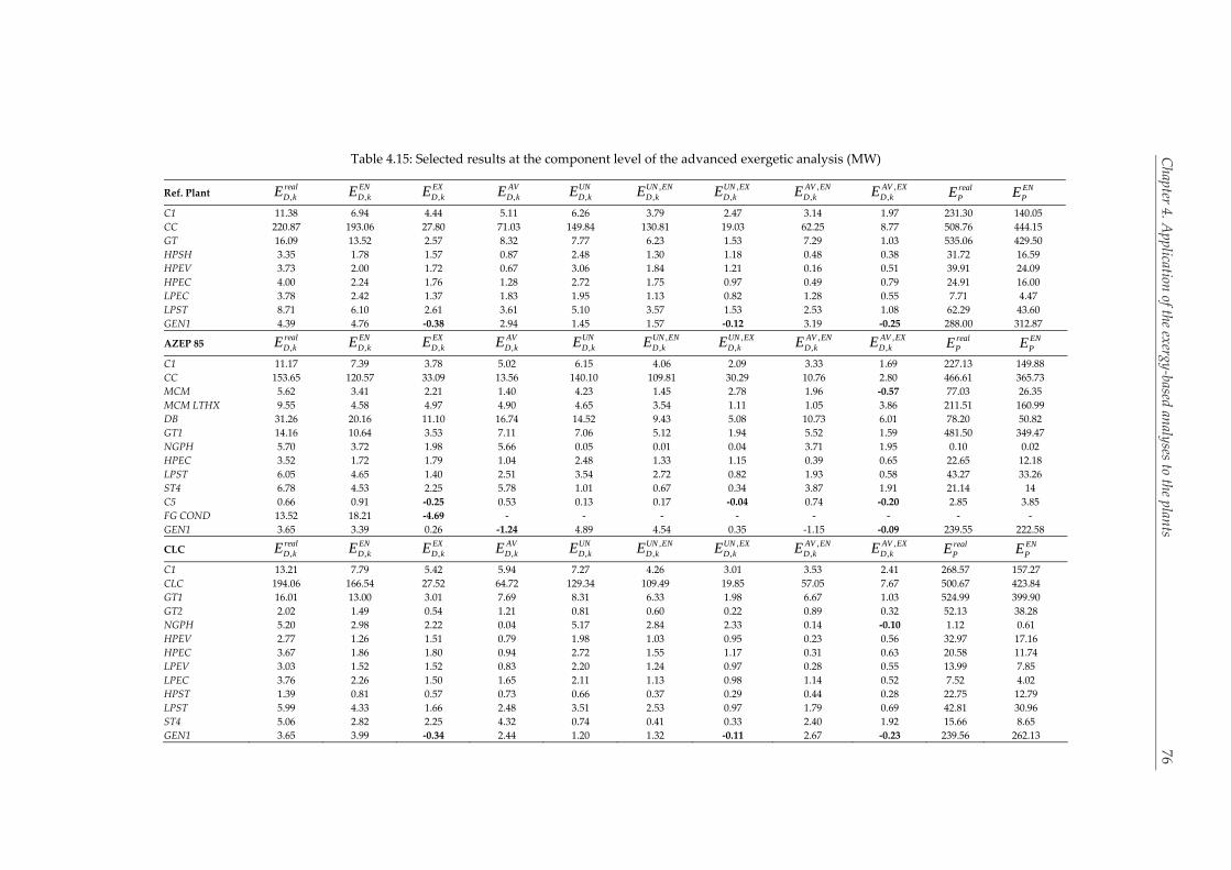
Chapter 4. Application of the exergy‐based analyses to the plants 76
Table 4.15: Selected results at the component level of the advanced exergetic analysis (MW)
Ref. Plant ,realD kE ,
END kE ,
EXD kE ,
AVD kE ,
UND kE
,,
UN END kE
,,
UN EXD kE
,,
AV END kE
,,
AV EXD kE
realPE
ENPE
C1 11.38 6.94 4.44 5.11 6.26 3.79 2.47 3.14 1.97 231.30 140.05
CC 220.87 193.06 27.80 71.03 149.84 130.81 19.03 62.25 8.77 508.76 444.15
GT 16.09 13.52 2.57 8.32 7.77 6.23 1.53 7.29 1.03 535.06 429.50
HPSH 3.35 1.78 1.57 0.87 2.48 1.30 1.18 0.48 0.38 31.72 16.59
HPEV 3.73 2.00 1.72 0.67 3.06 1.84 1.21 0.16 0.51 39.91 24.09
HPEC 4.00 2.24 1.76 1.28 2.72 1.75 0.97 0.49 0.79 24.91 16.00
LPEC 3.78 2.42 1.37 1.83 1.95 1.13 0.82 1.28 0.55 7.71 4.47
LPST 8.71 6.10 2.61 3.61 5.10 3.57 1.53 2.53 1.08 62.29 43.60
GEN1 4.39 4.76 ‐0.38 2.94 1.45 1.57 ‐0.12 3.19 ‐0.25 288.00 312.87
AZEP 85 ,realD kE ,
END kE ,
EXD kE ,
AVD kE ,
UND kE
,,
UN END kE
,,
UN EXD kE
,,
AV END kE
,,
AV EXD kE
realPE
ENPE
C1 11.17 7.39 3.78 5.02 6.15 4.06 2.09 3.33 1.69 227.13 149.88
CC 153.65 120.57 33.09 13.56 140.10 109.81 30.29 10.76 2.80 466.61 365.73
MCM 5.62 3.41 2.21 1.40 4.23 1.45 2.78 1.96 ‐0.57 77.03 26.35
MCM LTHX 9.55 4.58 4.97 4.90 4.65 3.54 1.11 1.05 3.86 211.51 160.99
DB 31.26 20.16 11.10 16.74 14.52 9.43 5.08 10.73 6.01 78.20 50.82
GT1 14.16 10.64 3.53 7.11 7.06 5.12 1.94 5.52 1.59 481.50 349.47
NGPH 5.70 3.72 1.98 5.66 0.05 0.01 0.04 3.71 1.95 0.10 0.02
HPEC 3.52 1.72 1.79 1.04 2.48 1.33 1.15 0.39 0.65 22.65 12.18
LPST 6.05 4.65 1.40 2.51 3.54 2.72 0.82 1.93 0.58 43.27 33.26
ST4 6.78 4.53 2.25 5.78 1.01 0.67 0.34 3.87 1.91 21.14 14
C5 0.66 0.91 ‐0.25 0.53 0.13 0.17 ‐0.04 0.74 ‐0.20 2.85 3.85
FG COND 13.52 18.21 ‐4.69 ‐ ‐ ‐ ‐ ‐ ‐ ‐ ‐
GEN1 3.65 3.39 0.26 ‐1.24 4.89 4.54 0.35 ‐1.15 ‐0.09 239.55 222.58
CLC ,realD kE ,
END kE ,
EXD kE ,
AVD kE ,
UND kE
,,
UN END kE
,,
UN EXD kE
,,
AV END kE
,,
AV EXD kE
realPE
ENPE
C1 13.21 7.79 5.42 5.94 7.27 4.26 3.01 3.53 2.41 268.57 157.27
CLC 194.06 166.54 27.52 64.72 129.34 109.49 19.85 57.05 7.67 500.67 423.84
GT1 16.01 13.00 3.01 7.69 8.31 6.33 1.98 6.67 1.03 524.99 399.90
GT2 2.02 1.49 0.54 1.21 0.81 0.60 0.22 0.89 0.32 52.13 38.28
NGPH 5.20 2.98 2.22 0.04 5.17 2.84 2.33 0.14 ‐0.10 1.12 0.61
HPEV 2.77 1.26 1.51 0.79 1.98 1.03 0.95 0.23 0.56 32.97 17.16
HPEC 3.67 1.86 1.80 0.94 2.72 1.55 1.17 0.31 0.63 20.58 11.74
LPEV 3.03 1.52 1.52 0.83 2.20 1.24 0.97 0.28 0.55 13.99 7.85
LPEC 3.76 2.26 1.50 1.65 2.11 1.13 0.98 1.14 0.52 7.52 4.02
HPST 1.39 0.81 0.57 0.73 0.66 0.37 0.29 0.44 0.28 22.75 12.79
LPST 5.99 4.33 1.66 2.48 3.51 2.53 0.97 1.79 0.69 42.81 30.96
ST4 5.06 2.82 2.25 4.32 0.74 0.41 0.33 2.40 1.92 15.66 8.65
GEN1 3.65 3.99 ‐0.34 2.44 1.20 1.32 ‐0.11 2.67 ‐0.23 239.56 262.13
Chapter 4. A
pplication of the exergy‐based an
alyses to the plants
76

Chapter 4. Application of the exergy‐based analyses to the plants 77
4.2.1.3 Splitting the exogenous exergy destruction
Table 4.16: Splitting the exogenous rate of exergy destruction (MW) a
Ref. plant
Component, k Component, r
Component, k Component, r
CC 27.80 C1 5.59 LPST 2.61 CC 0.70
GT1 8.84 C1 0.19
LPST 3.39 GT1 1.07
SUM 25.67 (7.96) SUM 1.96 (4.57)
MX 2.14 MX 0.65
C1 4.44 CC 3.51 GT1 2.57 CC 1.12
GT1 0.29 C1 0.29
LPST 0.11 LPST 0.25
SUM 4.18 (6.78) SUM 2.22 (14.08)
MX 0.26 MX 0.35
AZEP 85
Component, k
Component, r
Component, k Component, r
CC 33.09 DB 0.05 GT1 3.53 CC 2.21
MCM LTHX 0.06 DB 0.01
C1 3.44 MCM LTHX 0.01
GT1 5.13 C1 0.15
MCM 0.06 MCM 0.02
ST4 0.81 ST4 0.10
LPST 1.66 LPST 0.16
SUM 24.68 (‐5.86) SUM 3.34 (11.78)
MX 8.41 MX 0.19
DB 11.10 CC 4.27 MCM 2.21 CC 0.66
MCM LTHX 0.01 DB 0.03
C1 0.46 MCM LTHX ‐0.02
GT1 0.71 C1 0.07
MCM 0.01 GT1 0.19
ST4 0.18 ST4 0.03
LPST 0.35 LPST 0.07
SUM 8.18 (0.26) SUM 1.65 (0.57)
MX 2.92 MX 0.56
MCM LTHX 4.97 CC 0.76 ST4 2.25 CC ‐1.17
DB 0.04 DB 0.01
C1 ‐0.27 MCM LTHX 0.07
GT1 0.23 C1 0.31
MCM ‐0.20 GT1 0.14
ST4 0.11 MCM 0.16
LPST ‐0.10 LPST 0.05
SUM 2.84 (0.24) SUM 1.85 (1.77)
MX 2.13 MX 0.40
C1 3.78 CC 1.59 LPST 1.40 CC 0.39
DB 0.03 DB 0.04
MCM LTHX 0.01 MCM LTHX ‐0.10
GT1 0.27 C1 0.14
MCM 0.01 GT1 0.82
ST4 0.07 MCM 0.00
LPST 0.10 ST4 ‐0.25
SUM 2.88 (6.98) SUM 0.93 (0.54)
MX 0.91 MX 0.47
CLC plant
Component, k Component, r
Component, k Component, r
CLC 27.52 C1 3.13 ST4 2.25 C1 0.10
GT1 8.27 CLC 0.39
ST4 1.10 GT1 0.12
SUM 23.46 (12.81) SUM 1.63 (1.41)
MX 4.06 MX 0.62
C1 5.42 CLC 3.77 GT1 3.01 C1 0.34
GT1 0.35 CLC 1.36
ST4 0.05 ST4 0.08
SUM 4.65 (5.17) SUM 2.65 (14.23)
MX 0.78 MX 0.36 a The sum of exergy destruction caused by component k to the remaining components r is shown in parentheses
, EX
D kE ,,
EX rD kE ,
EXD kE ,
, EX r
D kE
, EX
D kE ,,
EX rD kE ,
EXD kE ,
, EX r
D kE
, EX
D kE ,,
EX rD kE ,
EXD kE ,
, EX r
D kE

Chapter 4. Application of the exergy‐based analyses to the plants 78
Although the exogenous exergy destruction accounts for a relatively small amount of the
exergy destruction in the plants, the determination of its specific sources can shed light onto
improvement options. Splitting the exogenous irreversibilities (also used in the calculation of
the mexogenous exergy destruction) requires additional simulations, because the components
are considered to operate under real conditions in pairs, while the necessary quantities are
calculated as defined in Chapter 3. The operating assumptions lead to a total of 2 2n n
simulations, with n being the number of the components in the plant.
The results for the components with the highest exogenous exergy destruction of the
plants and their mexogenous values (MX) are shown in Table 4.16. Four components have
been chosen from the reference and CLC plants and eight from the AZEP 85 to be explained
here. The complete results can be found in the supplemental data. As shown, the mexogenous
values are relatively low for all of the plants. The highest difference between the starting
results of the exogenous exergy destruction and the amount calculated through the splitting
is found for the reactors, while for the remaining components, the mexogenous values are
small. In the AZEP 85 the mexogenous exergy destruction of the CC is higher, revealing more
intense component interactions. As shown in Table 4.16, 52%, 41% and 26% of the exogenous
exergy destruction in the reactors of the reference plant, the CLC plant and the CC of the
AZEP 85 stem from GT1 and C1, a small part of which is avoidable. Similarly, in GT1 and C1,
the exogenous exergy destruction is mainly imposed by the reactors. Nonetheless, a large part
of the exogenous exergy destruction stemming from the reactors is avoidable (32‐33% for GT1
in the reference and CLC plants and 52% in the AZEP 85 and approximately 44% for C1 in all
of the plants). It should be noted that the exogenous exergy destruction caused by GT1 is
higher than that caused by the reactors by 77% in the reference plant and by 12% in the CLC
plant (SUM, the value in parentheses in Table 4.16). In the AZEP 85, the exogenous exergy
destruction caused by the CC is found to be negative. This is a result mainly determined by
the components related to the CO2 capture. Inefficiencies in the CC result in an improvement
of GT2, and all of the components constituting the CO2 compression unit. This contradicts the
results of the reference and CLC plants, but it is justified with the more complex structure of
the plant and the stronger interrelations of its components.
4.2.1.4 Calculating the total avoidable rate of exergy destruction
To better understand the improvement potential of the components, the variable ,,
AVD kE , as
stated in Equation (3.28) has been calculated (Table 4.17). The total avoidable exergy
destruction of component k, consists of both its avoidable endogenous and avoidable
exogenous exergy destruction caused by it to the remaining components of the plant. When
this value is high, the component is considered to have a large influence on the overall
system.
In the reference plant, the avoidable exogenous exergy destruction of GT1 is 34% higher
than that of the CC, in the CLC the two values are similar (with the exergy destruction of GT1
14% lower than that of the CLC reactors) and in the AZEP 85 both the CC and the DB have
negative avoidable exogenous values. In the reference and CLC plants, due to the
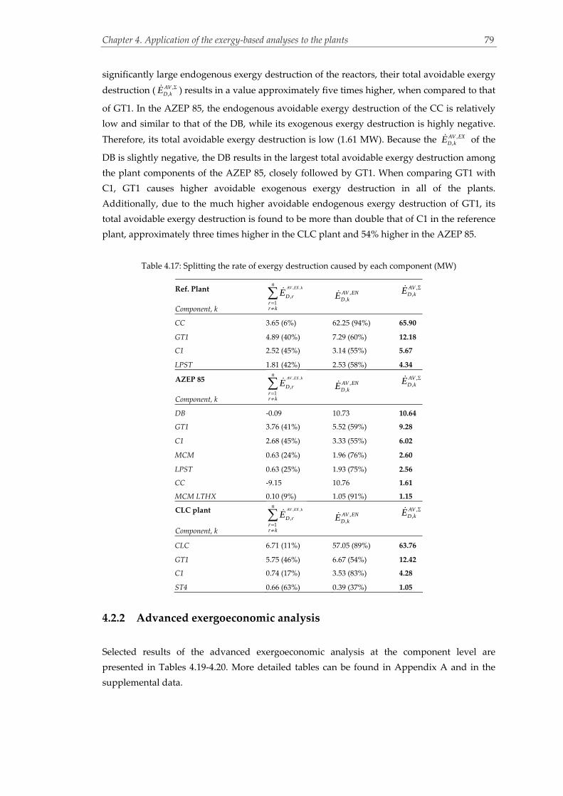
Chapter 4. Application of the exergy‐based analyses to the plants 79
significantly large endogenous exergy destruction of the reactors, their total avoidable exergy
destruction ( ,,
AVD kE ) results in a value approximately five times higher, when compared to that
of GT1. In the AZEP 85, the endogenous avoidable exergy destruction of the CC is relatively
low and similar to that of the DB, while its exogenous exergy destruction is highly negative.
Therefore, its total avoidable exergy destruction is low (1.61 MW). Because the ,,
AV EXD kE of the
DB is slightly negative, the DB results in the largest total avoidable exergy destruction among
the plant components of the AZEP 85, closely followed by GT1. When comparing GT1 with
C1, GT1 causes higher avoidable exogenous exergy destruction in all of the plants.
Additionally, due to the much higher avoidable endogenous exergy destruction of GT1, its
total avoidable exergy destruction is found to be more than double that of C1 in the reference
plant, approximately three times higher in the CLC plant and 54% higher in the AZEP 85.
Table 4.17: Splitting the rate of exergy destruction caused by each component (MW)
Ref. Plant
Component, k
, ,
,1
AV EX kn
D rrr k
E
,,
AV END kE
,,
AVD kE
CC 3.65 (6%) 62.25 (94%) 65.90
GT1 4.89 (40%) 7.29 (60%) 12.18
C1 2.52 (45%) 3.14 (55%) 5.67
LPST 1.81 (42%) 2.53 (58%) 4.34
AZEP 85
Component, k
, ,
,1
AV EX kn
D rrr k
E
,,
AV END kE
,,
AVD kE
DB ‐0.09 10.73 10.64
GT1 3.76 (41%) 5.52 (59%) 9.28
C1 2.68 (45%) 3.33 (55%) 6.02
MCM 0.63 (24%) 1.96 (76%) 2.60
LPST 0.63 (25%) 1.93 (75%) 2.56
CC ‐9.15 10.76 1.61
MCM LTHX 0.10 (9%) 1.05 (91%) 1.15
CLC plant
Component, k
, ,
,1
AV EX kn
D rrr k
E
,,
AV END kE
,,
AVD kE
CLC 6.71 (11%) 57.05 (89%) 63.76
GT1 5.75 (46%) 6.67 (54%) 12.42
C1 0.74 (17%) 3.53 (83%) 4.28
ST4 0.66 (63%) 0.39 (37%) 1.05
4.2.2 Advanced exergoeconomic analysis
Selected results of the advanced exergoeconomic analysis at the component level are
presented in Tables 4.19‐4.20. More detailed tables can be found in Appendix A and in the
supplemental data.
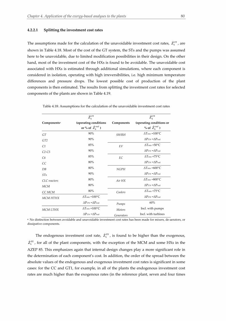
Chapter 4. Application of the exergy‐based analyses to the plants 80
4.2.2.1 Splitting the investment cost rates
The assumptions made for the calculation of the unavoidable investment cost rates, UNkZ , are
shown in Table 4.18. Most of the cost of the GT system, the STs and the pumps was assumed
here to be unavoidable, due to limited modification possibilities in their design. On the other
hand, most of the investment cost of the HXs is found to be avoidable. The unavoidable cost
associated with HXs is estimated through additional simulations, where each component is
considered in isolation, operating with high irreversibilities, i.e. high minimum temperature
differences and pressure drops. The lowest possible cost of production of the plant
components is then estimated. The results from splitting the investment cost rates for selected
components of the plants are shown in Table 4.19.
Table 4.18: Assumptions for the calculation of the unavoidable investment cost rates
UNkZ
UNkZ
Componentsa (operating conditions
or % of realkZ )
Components (operating conditions or
% of realkZ )
GT 90% SH/RH ΔTmin =100°C
GT2 90% ΔPUN =ΔPreal
C1 85% EV ΔTmin =50°C
C2‐C5 90% ΔPUN =ΔPreal
C6 85% EC ΔTmin =75°C
CC 80% ΔPUN =ΔPreal
DB 80% NGPH ΔTmin =600°C
STs 90% ΔPUN =ΔPreal
CLC reactors 80% Air HX ΔTmin =800°C
MCM 80% ΔPUN =ΔPreal
CC MCM 80% Coolers ΔTmin =75°C
MCM HTHX ΔTmin =100°C ΔPUN =ΔPreal
ΔPUN =ΔPreal Pumps 60%
MCM LTHX ΔTmin =100°C Motors Incl. with pumps
ΔPUN =ΔPreal Generators Incl. with turbines
a No distinction between avoidable and unavoidable investment cost rates has been made for mixers, de‐aerators, or
dissipative components.
The endogenous investment cost rate, ENkZ , is found to be higher than the exogenous,
EXkZ , for all of the plant components, with the exception of the MCM and some HXs in the
AZEP 85. This emphasizes again that internal design changes play a more significant role in
the determination of each component’s cost. In addition, the order of the spread between the
absolute values of the endogenous and exogenous investment cost rates is significant in some
cases: for the CC and GT1, for example, in all of the plants the endogenous investment cost
rates are much higher than the exogenous rates (in the reference plant, seven and four times
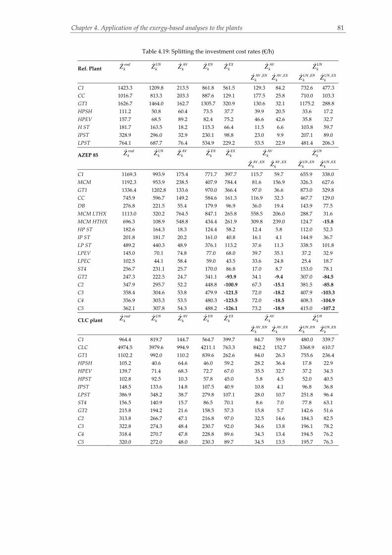
Chapter 4. Application of the exergy‐based analyses to the plants 81
Table 4.19: Splitting the investment cost rates (€/h)
Ref. Plant realkZ UN
kZ AVkZ
ENkZ EX
kZ AVkZ
UNkZ
,AV EN
kZ ,AV EXkZ
,UN ENkZ ,UN EX
kZ
C1 1423.3 1209.8 213.5 861.8 561.5 129.3 84.2 732.6 477.3
CC 1016.7 813.3 203.3 887.6 129.1 177.5 25.8 710.0 103.3
GT1 1626.7 1464.0 162.7 1305.7 320.9 130.6 32.1 1175.2 288.8
HPSH 111.2 50.8 60.4 73.5 37.7 39.9 20.5 33.6 17.2
HPEV 157.7 68.5 89.2 82.4 75.2 46.6 42.6 35.8 32.7
H ST 181.7 163.5 18.2 115.3 66.4 11.5 6.6 103.8 59.7
IPST 328.9 296.0 32.9 230.1 98.8 23.0 9.9 207.1 89.0
LPST 764.1 687.7 76.4 534.9 229.2 53.5 22.9 481.4 206.3
AZEP 85 realkZ UN
kZ AVkZ
ENkZ EX
kZ AVkZ
UNkZ
,AV EN
kZ ,AV EXkZ
,UN ENkZ ,UN EX
kZ
C1 1169.3 993.9 175.4 771.7 397.7 115.7 59.7 655.9 338.0
MCM 1192.3 953.9 238.5 407.9 784.4 81.6 156.9 326.3 627.6
GT1 1336.4 1202.8 133.6 970.0 366.4 97.0 36.6 873.0 329.8
CC 745.9 596.7 149.2 584.6 161.3 116.9 32.3 467.7 129.0
DB 276.8 221.5 55.4 179.9 96.9 36.0 19.4 143.9 77.5
MCM LTHX 1113.0 320.2 764.5 847.1 265.8 558.5 206.0 288.7 31.6
MCM HTHX 696.3 108.9 548.8 434.4 261.9 309.8 239.0 124.7 ‐15.8
HP ST 182.6 164.3 18.3 124.4 58.2 12.4 5.8 112.0 52.3
IP ST 201.8 181.7 20.2 161.0 40.8 16.1 4.1 144.9 36.7
LP ST 489.2 440.3 48.9 376.1 113.2 37.6 11.3 338.5 101.8
LPEV 145.0 70.1 74.8 77.0 68.0 39.7 35.1 37.2 32.9
LPEC 102.5 44.1 58.4 59.0 43.5 33.6 24.8 25.4 18.7
ST4 256.7 231.1 25.7 170.0 86.8 17.0 8.7 153.0 78.1
GT2 247.3 222.5 24.7 341.1 ‐93.9 34.1 ‐9.4 307.0 ‐84.5
C2 347.9 295.7 52.2 448.8 ‐100.9 67.3 ‐15.1 381.5 ‐85.8
C3 358.4 304.6 53.8 479.9 ‐121.5 72.0 ‐18.2 407.9 ‐103.3
C4 356.9 303.3 53.5 480.3 ‐123.5 72.0 ‐18.5 408.3 ‐104.9
C5 362.1 307.8 54.3 488.2 ‐126.1 73.2 ‐18.9 415.0 ‐107.2
CLC plant realkZ UN
kZ AVkZ
ENkZ EX
kZ AVkZ
UNkZ
,AV EN
kZ ,AV EXkZ
,UN ENkZ ,UN EX
kZ
C1 964.4 819.7 144.7 564.7 399.7 84.7 59.9 480.0 339.7
CLC 4974.5 3979.6 994.9 4211.1 763.3 842.2 152.7 3368.9 610.7
GT1 1102.2 992.0 110.2 839.6 262.6 84.0 26.3 755.6 236.4
HPSH 105.2 40.6 64.6 46.0 59.2 28.2 36.4 17.8 22.9
HPEV 139.7 71.4 68.3 72.7 67.0 35.5 32.7 37.2 34.3
HPST 102.8 92.5 10.3 57.8 45.0 5.8 4.5 52.0 40.5
IPST 148.5 133.6 14.8 107.5 40.9 10.8 4.1 96.8 36.8
LPST 386.9 348.2 38.7 279.8 107.1 28.0 10.7 251.8 96.4
ST4 156.5 140.9 15.7 86.5 70.1 8.6 7.0 77.8 63.1
GT2 215.8 194.2 21.6 158.5 57.3 15.8 5.7 142.6 51.6
C2 313.8 266.7 47.1 216.8 97.0 32.5 14.6 184.3 82.5
C3 322.8 274.3 48.4 230.7 92.0 34.6 13.8 196.1 78.2
C4 318.4 270.7 47.8 228.8 89.6 34.3 13.4 194.5 76.2
C5 320.0 272.0 48.0 230.3 89.7 34.5 13.5 195.7 76.3

Chapter 4. Application of the exergy‐based analyses to the plants
82
higher, in the CLC plant five and three times higher and in the AZEP 85 four and three times
higher for the CC and GT1, respectively). For the compressor, this difference is smaller. Some
HXs in all of the plants, as well as the CO2 compressors in the AZEP 85 result in a ENkZ that is
higher than the realkZ . This is again related to increased mass flow rates in the endogenous
case, when compared to the real process, which results in a higher rate of product exergy. The
interpretation of these results is that the cost of a component with negative EXkZ increases
when all other components operate under theoretical conditions. Thus, to decrease its cost,
the irreversibilities within the other components must be increased.
The results from splitting the investment cost rates indicate that, priority should be given
to the GT system, with the reactors first, C1 second and GT1 third for the CLC plant and C1
first, CC second and GT1 third for the reference plant. These components have the highest
avoidable cost rates, while the components that follow priority‐wise, in the reference and
CLC plants, are the HXs of the high and low‐pressure HRSG (ranking varies among the
HPSH, HPEV and the LPEV). On the other hand, in the AZEP 85 priority should be given to
the two HXs of the MCM reactor, the MCM, C1, the CC and then to GT1.
Since the components with the larger investment cost rates, kZ , are the main
turbomachinery and the reactors and their investment cost is mainly unavoidable, the
investment cost rate of the plant is largely unavoidable. Additionally, most of the exogenous
values are relatively low, when compared to the endogenous values, showing that
components interactions are not as important as the internal operation of the components.
Specifically, 64‐87% and 73‐80% of the investment cost of the reactors and GT1, respectively,
can be avoided through operating changes in the components themselves.
4.2.2.2 Splitting the cost rate of exergy destruction
The calculations used for splitting the cost of exergy destruction, ,D kC , are based on the
equations shown in Table 3.1. The results for selected components of the plants are shown in
Table 4.20.
In all of the plants, the majority of the HXs, the LPST, the reactors (with the exception of
the DB) and C1, present high rates of unavoidable exergy destruction. The opposite is true for
GT1, the CO2 compressors, the high‐ and intermediate‐pressure ST. The highest values of
both avoidable and unavoidable rate of exergy destruction are found for the reactors, GT1, C1
and the LPST. In the case of the reference plant, the LPST presents a 13% higher avoidable
cost rate of exergy destruction when compared to that of C1.
In the reference and CLC plants, more than 67% of the total cost rate of exergy
destruction of the reactors is considered unavoidable, while for the CC of the AZEP 85 this
percentage reaches 91%. Yet, the absolute values of the avoidable cost rates of exergy
destruction associated with these components are significantly larger than other plant
components, with the exception of the CC in the AZEP 85 that results in a lower value than
GT1 and the DB. Furthermore, 65‐87% of the unavoidable cost of the reactors is endogenous.
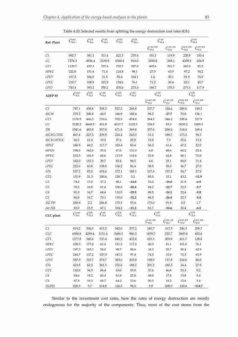
Chapter 4. Application of the exergy‐based analyses to the plants
83
Table 4.20: Selected results from splitting the exergy destruction cost rates (€/h)
Ref. Plant ,realD kC ,
UND kC ,
AVD kC ,
END kC ,
EXD kC ,
AVD kC ,
UND kC
,
,AV END kC ,
,AV EXD kC
,,
UN END kC ,
,UN EXD kC
C1 692.7 381.3 311.4 422.3 270.4 191.5 119.9 230.9 150.4
CC 7276.3 4936.4 2339.9 6360.4 916.0 2050.8 289.1 4309.5 626.9
GT1 1139.7 432.3 707.4 752.7 387.0 405.6 301.7 347.0 85.3
HPEC 222.8 151.4 71.4 124.8 98.1 27.5 43.9 97.2 54.2
LPEV 197.5 166.0 31.5 93.4 104.1 1.4 30.1 91.9 74.0
LPEC 210.7 108.8 101.9 134.6 76.1 71.5 30.4 63.1 45.7
LPST 743.4 393.2 350.2 470.0 273.4 194.7 155.5 275.3 117.9
AZEP 85 ,realD kC ,
UND kC ,
AVD kC ,
END kC ,
EXD kC ,
AVD kC ,
UND kC
,
,AV END kC ,
,AV EXD kC
,,
UN END kC ,
,UN EXD kC
C1 797.1 438.8 358.3 527.2 269.8 237.7 120.6 289.6 149.2
MCM 275.3 206.8 68.5 166.9 108.4 96.2 ‐27.7 70.8 136.1
GT1 1176.9 466.3 710.6 702.9 474.0 364.5 346.2 338.4 127.9
CC 5120.2 4668.5 451.8 4017.7 1102.5 358.5 93.3 3659.2 1009.3
DB 1041.6 483.8 557.8 671.8 369.8 357.4 200.4 314.4 169.4
MCM LTHX 467.4 227.5 239.9 224.4 243.0 51.2 188.7 173.2 54.3
MCM HTHX 60.5 41.0 19.5 37.6 22.9 12.0 7.5 25.6 15.4
HPST 186.9 69.2 117.7 103.4 83.4 56.3 61.4 47.2 22.0
HPSH 198.0 142.6 55.4 67.0 131.0 6.8 48.6 60.2 82.4
HPEC 232.5 163.9 68.6 113.9 118.6 25.8 42.8 88.1 75.8
LPEV 182.0 152.3 29.7 85.4 96.5 4.6 25.1 80.8 71.4
LPEC 222.6 63.8 158.8 136.2 86.4 99.5 59.3 36.7 27.0
ST4 557.2 82.5 474.6 372.1 185.1 317.4 157.2 54.7 27.9
GT2 131.9 31.3 100.6 128.7 3.2 85.5 15.1 43.2 ‐11.9
C2 74.2 17.0 57.2 98.1 ‐24.0 76.2 ‐19.0 21.9 ‐4.9
C3 78.2 16.8 61.4 106.6 ‐28.4 84.2 ‐22.7 22.5 ‐5.7
C4 81.0 16.7 64.4 110.9 ‐29.9 88.5 ‐24.1 22.4 ‐5.8
C5 86.8 16.7 70.1 119.0 ‐32.2 96.5 ‐26.4 22.5 ‐5.8
NG PH 268.9 2.2 266.8 175.5 93.4 175.0 91.8 0.5 1.7
Air HX 83.0 15.9 67.1 104.2 ‐21.2 81.7 ‐14.6 22.4 ‐6.5
CLC plant ,realD kC ,
UND kC ,
AVD kC ,
END kC ,
EXD kC ,
AVD kC ,
UND kC
,
,AV END kC ,
,AV EXD kC
,,
UN END kC ,
,UN EXD kC
C1 919.2 506.0 413.2 542.0 377.2 245.7 167.5 296.3 209.7
CLC 6390.8 4259.4 2131.4 5484.5 906.3 1878.7 252.7 3605.8 653.6
GT1 1277.8 540.4 737.4 845.2 432.6 433.5 303.9 411.7 128.8
HPEC 238.5 177.0 61.4 121.2 117.2 20.3 41.1 101.0 76.1
LPEV 197.3 143.3 54.0 98.7 98.6 18.3 35.7 80.4 62.9
LPEC 244.7 137.2 107.5 147.3 97.4 74.0 33.6 73.3 63.9
LPST 587.3 310.7 276.7 383.6 203.8 158.9 117.8 224.6 86.0
ST4 423.8 62.3 361.5 235.6 188.2 201.2 160.3 34.4 27.9
GT2 118.9 34.5 84.4 63.0 55.9 37.6 46.8 25.3 9.2
C4 84.6 19.2 65.4 61.8 22.8 48.0 17.4 13.8 5.4
C5 87.8 19.2 68.7 64.3 23.6 50.5 18.2 13.8 5.4
NGPH 220.5 5.7 214.8 126.3 94.2 5.9 208.9 120.4 ‐114.7
Similar to the investment cost rates, here the rates of exergy destruction are mostly
endogenous for the majority of the components. Thus, most of the cost stems from the

Chapter 4. Application of the exergy‐based analyses to the plants
84
operation of the components themselves and component interactions are of lower
importance.
Evaluating the results of the sources of the cost of exergy destruction, the reference plant
can potentially be improved through improvement of the CC, GT1, the LPST and C1. On the
other hand, in the CLC plant, priority should be given to the CLC first, GT1 second, C1 third
and last ST4. In the AZEP 85 the component with the highest avoidable cost of exergy
destruction is GT1, followed by the DB, ST4 and then the CC.
4.2.2.3 Splitting the exogenous cost rates of investment and exergy destruction
Although the exogenous costs are of relatively low significance when compared to the
endogenous costs, their sources can reveal additional improvement potential for the overall
plant. The splitting of the exogenous costs for the components with the highest investment‐
related cost and exergy destruction‐related costs is shown in Tables 4.21 and 4.22,
respectively.
The main source of the exogenous investment cost rate for the reactors is GT1, with the
exception of the DB in the AZEP 85 that is influenced more by the CC. The main source of the
exogenous investment cost rate for C1 and GT1 of all plants is the reactors. The mexogenous
cost, that is the cost difference between the calculated exogenous cost (shown in Tables 4.21
and 4.22) and the sum of the split parts caused to each of the remaining components
(complete tables can be found in the supplemental data), is found to be very high for the
MCM and the MCM LTHX because of their intense interaction.
The effect of the chemical reactors on the remaining components is critical, since they are
responsible for large parts of the costs in other components. The reactors first and GT1
second, cause relatively high total exogenous costs in the CLC plant (SUM, values in
parentheses in Tables 4.21 and 4.22), while the same is true for the investment cost rates of the
reference plant. GT1 causes a higher exogenous cost rate of exergy destruction than the CC in
the reference plant (SUM, values in parentheses in Table 4.22). In the AZEP 85, GT1 causes
the highest rate of investment cost, followed by C1, the MCM HTHX (436.7 €/h) and the
MCM (because of their large influence on the CO2 compressors), while the exogenous
investment cost of the CC is relatively low, due to its negative effect on other components
(mainly those processing the CO2 stream). Also, in the AZEP 85, GT1 causes the highest
exogenous cost rate of exergy destruction, while the CC, has a negative exogenous value of
exergy destruction, due to the inverse relationship between its efficiency and that of other
equipment.

Chapter 4. Application of the exergy‐based analyses to the plants
85
Table 4.21: Selected results from splitting the exogenous investment cost rate (€/h)a
Ref. plant Component, k EXkZ Component, r
, EX rkZ Component, k
EXkZ Component, r
, EX rkZ
CC 129.11 C1 24.62 LPST 229.19 CC 61.69
GT1 40.65 C1 16.31
LPST 15.58 GT1 93.66
SUM 116.90 (741.68) SUM 172.17 (68.57)
MX 12.22 MX 57.02
C1 561.51 CC 416.85 GT1 1305.74 CC 156.23
GT1 36.39 C1 41.23
LPST 13.98 LPST 24.15
SUM 500.58 (110.47) SUM 275.42 (352.64)
MX 60.93 MX 45.51
AZEP 85 Component, r EXkZ Component, r
, EX rkZ
Component, r EXkZ Component, r
, EX rkZ
CC 161.26 DB 0.22 GT1 366.45 CC 202.46
MCM LTHX 0.28 DB 1.18
C1 16.70 MCM LTHX 0.78
GT1 24.87 C1 27.34
MCM 0.48 MCM 1.47
ST4 3.94 ST4 9.24
LPST 8.05 LPST 14.51
SUM 105.69 (138.96) SUM 328.52 (757.44)
MX 55.57 MX 37.92
DB 96.93 CC 37.55 MCM 784.44 CC 114.35
MCM LTHX 0.08 DB 17.88
C1 4.29 MCM LTHX 13.17
GT1 6.33 C1 ‐8.89
MCM 0.13 GT1 3.47
ST4 1.65 ST4 3.86
LPST 3.11 LPST 25.36
SUM 80.76 (403.28) SUM 452.41 (430.00)
MX 16.17 MX 332.03
MCM LTHX 265.85 CC 28.82 ST4 86.76 CC ‐43.98
DB 44.11 DB 0.47
C1 31.80 MCM LTHX 2.73
GT1 77.08 C1 11.76
MCM ‐99.30 GT1 6.04
ST4 53.97 MCM 5.88
LPST ‐82.20 LPST 2.05
SUM ‐34.14 (357.00) SUM 70.49 (405.77)
MX 299.98 MX 16.28
C1 397.70 CC 166.14 LPST 113.16 CC 31.38
DB 4.39 DB 3.02
MCM LTHX 1.12 MCM LTHX ‐7.79
GT1 27.86 C1 11.08
MCM 1.54 GT1 66.52
ST4 7.54 MCM 0.00
LPST 10.10 ST4 ‐0.25
SUM 302.97 (611.92) SUM 75.58 (329.87)
MX 94.73 MX 37.57
CLC plant Component, k EXkZ Component, r
, EX rkZ Component, k
EXkZ Component, r
, EX rkZ
CLC 763.33 C1 141.71 ST4 70.06 C1 3.09
GT1 209.03 CLC 12.02
ST4 27.77 GT1 3.78
SUM 655.70 (667.11) SUM 50.53 (30.94)
MX 107.64 MX 19.52
C1 399.66 CLC 278.97 GT1 262.62 C1 31.50
GT1 25.40 CLC 122.79
ST4 3.39 ST4 5.11
SUM 342.58 (246.67) SUM 215.32 (478.35)
MX 57.09 MX 47.30 a In parentheses the sum of exergy destruction caused by component k to the remaining components r is shown

Chapter 4. Application of the exergy‐based analyses to the plants
86
Table 4.22: Selected results from splitting the exogenous cost rates of exergy destruction (€/h) a
Ref. plant Component, k ,EXD kC Component, r
,,
EX rD kC Component, k ,
EXD kC Component, r
,,
EX rD kC
CC 915.97 C1 184.26 LPST 273.40 CC 54.20
GT1 291.31 C1 14.333
LPST 111.65 GT1 82.276
SUM 845.53 (488.33) SUM 151.23 (175.24)
MX 70.44 MX 122.17
C1 270.36 CC 213.62 GT1 752.65 CC 62.20
GT1 17.84 C1 16.414
LPST 6.85 LPST 13.921
SUM 254.65 (256.93) SUM 123.55 (625.37)
MX 15.70 MX 263.49
AZEP 85
Component, k ,
EXD kC
Component, r ,
, EX r
D kC
Component, k ,
EXD kC
Component, r ,
, EX r
D kC
CC 1102.53 DB 1.51 GT1 474.05 CC 145.81
MCM LTHX 1.90 DB 0.43
C1 114.59 MCM LTHX 0.50
GT1 170.92 C1 9.69
MCM 2.15 MCM 1.02
ST4 27.11 ST4 6.70
LPST 55.32 LPST 10.51
SUM 822.32(‐560.5) SUM 220.70 (605.62)
MX 280.21 MX 253.35
DB 369.78 CC 142.13 MCM 108.37 CC 32.14
MCM LTHX 0.22 DB 1.67
C1 15.45 MCM LTHX ‐1.09
GT1 23.63 C1 3.39
MCM 0.36 GT1 9.11
ST4 6.15 ST4 1.58
LPST 11.74 LPST 3.37
SUM 272.45 (16.80) SUM 80.85 (33.25)
MX 97.33 MX 27.51
MCM LTHX 243.02 CC 37.21 ST4 185.09 CC ‐95.71
DB 2.05 DB 1.02
C1 ‐13.05 MCM LTHX 5.98
GT1 11.24 C1 25.70
MCM ‐9.92 GT1 11.88
ST4 5.35 MCM 12.87
LPST ‐4.77 LPST 4.48
SUM 138.75 (10.08) SUM 151.85 (76.26)
MX 104.27 MX 33.24
C1 269.82 CC 113.52 LPST 179.60 CC 34.02
DB 1.79 DB 3.27
MCM LTHX 0.53 MCM LTHX ‐8.46
GT1 19.04 C1 12.01
MCM 0.76 GT1 72.12
ST4 5.15 MCM 0.00
LPST 6.90 ST4 ‐0.25
SUM 205.15 (350.05) SUM 81.70 (109.45)
MX 64.67 MX 103.39
CLC plant Component, k ,EXD kC Component, r
,,
EX rD kC Component, k ,
EXD kC Component, r
,,
EX rD kC
CLC 906.30 C1 103.23 ST4 188.20 C1 8.43
GT1 272.24 CLC 32.72
ST4 36.17 GT1 9.75
SUM 772.62 (813.84) SUM 136.13 (52.23)
MX 133.68 MX 52.07
C1 377.20 CLC 262.15 GT1 432.64 C1 22.37
GT1 24.38 CLC 88.40
ST4 3.25 ST4 5.14
SUM 323.20 (236.06) SUM 172.20 (689.31)
MX 54.00 MX 260.44 a In parentheses the sum of exergy destruction caused by component k to the remaining components r is shown

Chapter 4. Application of the exergy‐based analyses to the plants
87
4.2.2.4 Calculating the total avoidable cost rates associated with plant components
The total avoidable cost of component k is calculated through the addition of the avoidable
cost of exergy destruction or investment cost caused by its operation on the remaining
components and its endogenous cost of exergy destruction or investment cost. The results of
the most influential components of the plants are shown in Tables 4.23 and 4.24. The total
avoidable costs of component k are calculated using Equations (3.32)‐(3.36).
Table 4.23: Avoidable investment cost rate (€/h) Table 4.24: Avoidable exergy destruction cost rate (€/h)
Ref. Plant Ref. Plant
Component, k
, ,
1
AV EX kn
rrr k
Z
,AV ENkZ
,AVkZ
Component, k
, ,
,1
AV EX kn
D rrr k
C
,,
AV END kC
,,
AVD kC
CC 121.09 (40.6%) 177.51 (59.4%) 298.60 CC 170.37 (7.7%) 2,050.85 (92.3%) 2,221.22
GT1 74.80 (36.4%) 130.57 (63.6%) 205.38 GT1 156.63 (27.9) 405.64 (72.1) 562.27
C1 20.41 (13.6%) 129.27 (86.4%) 149.69 C1 84.82 (30.7) 191.45 (69.3) 276.27
LPST 12.71 (19.2%) 53.49 (80.8%) 66.21 LPST 51.15 (20.8) 194.71 (79.2) 245.87
AZEP 85 AZEP 85
Component, k
, ,
1
AV EX kn
rrr k
Z
,AV ENkZ
,AVkZ
Component, k
, ,
,1
AV EX kn
D rrr k
C
,,
AV END kC
,,
AVD kC
MCM LTHX 346.02 (38.3%) 558.49 (61.7%) 904.51 GT1 119.25 (24.7%) 364.45 (75.3%) 483.70
CC 720.80 (86.0%) 116.93 (14.0%) 837.73 DB ‐5.95 357.44 351.49
GT1 446.91 (82.2%) 97.00 (17.8%) 543.91 CC ‐26.49 358.53 332.04
MCM 398.52 (77.5%) 115.75 (22.5%) 514.27 C1 67.37 (22.1%) 237.68 (77.9%) 305.05
C1 391.29 (77.2%) 115.75 (22.8%) 507.04 LPST 44.69 (20.9%) 168.94 (79.1%) 213.63
DB 358.92 (90.9%) 35.98 (9.1%) 394.90 MCM 34.02 (26.1%) 96.16 (73.9%) 130.18
LPST 287.20 (88.4%) 37.61 (11.6%) 324.81 MCM LTHX 3.95 (7.2%) 51.23 (92.8%) 55.18
CLC Plant CLC Plant
Component, k
, ,
1
AV EX kn
rrr k
Z
,AV ENkZ
,AVkZ
Component, k
, ,
,1
AV EX kn
D rrr k
C
,,
AV END kC
,,
AVD kC
CLC 109.79 (11.5%) 842.23 (88.5%) 952.02 CLC 241.83 (11.4%) 1,878.68 (88.6%) 2,120.51
GT1 102.51 (55.0%) 83.96 (45.0%) 186.47 GT1 179.12 (29.2%) 433.52 (70.8%) 612.64
C1 47.07 (35.7%) 84.71 (64.3%) 131.78 C1 19.99 (7.5%) 245.71 (92.5%) 265.70
ST4 7.00 (44.7%) 8.65 (55.3%) 15.65 ST4 12.52 (5.9%) 201.17 (94.1%) 213.69
Among GT1, C1 and the reactors of the plants, the lowest avoidable exogenous investment
cost rate is calculated for C1. The avoidable endogenous costs are similar for C1 and GT1 in
the reference and CLC plants, while in the AZEP 85, C1 has a 19% higher cost rate.
Nonetheless, C1 has lower total cost rates in all of the plants. It should be noted that GT1 and
the reactors of the CLC plant cause similar total avoidable exogenous investment cost rates
(first column in Table 4.23), but the reactors have a much higher total cost rate due to their
significantly higher endogenous value.

Chapter 4. Application of the exergy‐based analyses to the plants
88
Table 4.25: Ranking of the components with the highest total avoidable cost rate, ,,
AVD kC + ,AV
kZ (€/h)
Component, k Ref. Plant Component, k AZEP 85 Component, k CLC Plant
CC 2,519.8 CC 1,169.8 CLC 3,072.5
GT1 767.7 GT1 1,027.6 GT1 799.1
C1 426.0 MCM LTHX 944.5 C1 397.5
LPST 312.1 C1 812.1 ST4 229.3
DB 746.4
MCM 644.5
LPST 538.4
While the differences in the investment cost rates are kept at relatively low levels, the
differences in the exergy destruction‐related costs show large spreads among the different
components. The avoidable exogenous cost of exergy destruction of GT1 and the CC in the
reference plant are relatively close. However, again, the significantly larger avoidable
endogenous cost of exergy destruction for the CC, results in an overall cost rate that is
approximately four times higher. C1 follows GT1 with an approximately two times lower
overall cost of exergy destruction. In the CLC plant, the reactors result in a 35% higher
avoidable exogenous cost rate of exergy destruction when compared to GT1 and since the
difference between the endogenous values of the components is much larger, the total cost
rate of the reactors is approximately three times higher. In the reference and CLC plants, the
avoidable exogenous cost caused by GT1 is the second highest. C1 follows GT1 in cost. In the
AZEP 85 the highest cost of avoidable exogenous exergy destruction is found for the MCM
HTHX (200.2 €/h), followed by GT1 and C1. However, due to its low avoidable endogenous
exergy destruction cost, the MCM HTHX has a low total avoidable cost and GT1 has the
highest total cost. The total avoidable cost of exergy destruction of the CC is relatively
reduced (ranked after GT1 and the DB) due to its negative avoidable exogenous cost rate.
The most important result of the component evaluation is the sum of the avoidable
exergy destruction and investment costs. As shown in Table 4.25, the cost of exergy
destruction is the main deciding parameter of the overall cost in the CLC and reference
plants. On the other hand, in the AZEP, both costs affect the overall results. In all of the
plants, the reactors are ranked first and GT1 second.
4.2.3 Advanced exergoenvironmental analysis
Selected results of the advanced exergoenvironmental analysis at the component level are
presented in Tables 4.26‐4.27. Detailed tables can be found in Appendix A and in the
supplemental data. In contrast to the advanced exergoeconomic analysis, in the advanced
exergoenvironmental analysis, the component‐related environmental impact has not been
split, due to its negligible influence on the total impact. Thus, here the environmental impacts
associated with exergy destruction and pollutant formation are split.

Chapter 4. Application of the exergy‐based analyses to the plants
89
4.2.3.1 Splitting the environmental impact of exergy destruction
Table 4.26: Selected results from splitting the environmental impact of exergy destruction (Pts/h)
Ref. Plant , real
D kB ,UN
D kB , AV
D kB , EN
D kB , EX
D kB , AV
D kB ,
UND kB
,
, AV EN
D kB ,
, AV EX
D kB
,,
UN END kB
,,
UN EXD kB
C1 69.36 38.18 31.18 42.29 27.07 19.17 12.01 23.12 15.06
CC 762.83 517.52 245.31 666.81 96.03 215.01 30.31 451.80 65.72
GT1 120.16 45.58 74.58 79.35 40.81 42.77 31.81 36.59 8.99
HPEC 23.49 15.96 7.53 13.15 10.34 2.90 4.63 10.25 5.71
LPEV 20.82 17.50 3.32 9.85 10.97 0.15 3.17 9.69 7.80
LPEC 22.21 11.47 10.74 14.19 8.02 7.54 3.21 6.66 4.82
LPST 69.86 36.95 32.91 44.17 25.69 18.30 14.61 25.87 11.08
AZEP 85 , real
D kB ,UN
D kB , AV
D kB , EN
D kB , EX
D kB , AV
D kB ,
UND kB
,
, AV EN
D kB ,
, AV EX
D kB
,,
UN END kB
,,
UN EXD kB
C1 69.66 38.35 31.31 46.08 23.58 20.77 10.54 25.31 13.04
MCM 28.66 21.53 7.13 17.38 11.28 10.01 ‐2.88 7.37 14.17
GT1 107.05 42.41 64.64 63.93 43.12 33.15 31.49 30.78 11.63
CC 536.81 489.44 47.36 421.22 115.59 37.59 9.78 383.63 105.81
DB 109.20 50.72 58.48 70.43 38.77 37.47 21.01 32.96 17.76
MCM LTHX 48.89 23.79 25.09 23.47 25.42 5.36 19.73 18.11 5.68
MCM HTHX 6.33 4.29 2.04 3.93 2.40 1.26 0.78 2.68 1.61
HPST 16.06 5.95 10.11 8.89 7.17 4.83 5.28 4.05 1.89
HPSH 18.01 12.97 5.04 6.10 11.92 0.62 4.42 5.48 7.50
HPEC 21.15 14.91 6.24 10.36 10.79 2.34 3.90 8.02 6.89
LPEV 16.55 13.85 2.70 7.77 8.78 0.42 2.28 7.35 6.50
LPEC 20.25 5.80 14.44 12.39 7.86 9.05 5.40 3.34 2.46
ST4 47.40 7.02 40.38 31.65 15.75 27.00 13.37 4.65 2.37
GT2 14.16 3.36 10.80 13.82 0.34 9.18 1.62 4.64 ‐1.28
C2 5.67 1.30 4.37 7.50 ‐1.83 5.83 ‐1.46 1.67 ‐0.38
C3 5.98 1.28 4.70 8.16 ‐2.17 6.44 ‐1.74 1.72 ‐0.44
C4 6.20 1.27 4.92 8.48 ‐2.29 6.77 ‐1.85 1.71 ‐0.44
C5 6.64 1.28 5.36 9.10 ‐2.47 7.38 ‐2.02 1.72 ‐0.44
NG PH 28.88 0.23 28.65 18.84 10.04 18.79 9.85 0.05 0.18
Air HX 8.91 1.71 7.20 11.19 ‐2.27 8.78 ‐1.57 2.41 ‐0.70
CLC plant , real
D kB ,UN
D kB , AV
D kB , EN
D kB , EX
D kB , AV
D kB ,
UND kB
,
, AV EN
D kB ,
, AV EX
D kB
,,
UN END kB
,,
UN EXD kB
C1 79.58 43.81 35.77 46.92 32.65 21.27 14.50 25.65 18.15
CLC 671.79 447.74 224.05 576.52 95.27 197.48 26.56 379.04 68.71
GT1 114.08 48.25 65.83 75.45 38.62 38.70 27.13 36.75 11.50
HPEC 21.29 15.80 5.48 10.82 10.46 1.81 3.67 9.01 6.79
LPEV 17.62 12.80 4.82 8.81 8.81 1.63 3.19 7.18 5.62
LPEC 21.85 12.25 9.60 13.15 8.70 6.61 3.00 6.54 5.70
LPST 47.97 25.37 22.60 31.33 16.64 12.98 9.62 18.35 7.02
ST4 34.97 5.14 29.82 19.44 15.53 16.60 13.23 2.84 2.30
GT2 11.37 3.30 8.07 6.02 5.35 3.60 4.47 2.42 0.88
C4 6.41 1.45 4.96 4.68 1.73 3.64 1.32 1.04 0.41
C5 6.65 1.45 5.20 4.87 1.78 3.82 1.38 1.04 0.41
NGPH 21.08 0.55 20.53 12.07 9.00 0.56 19.97 11.51 ‐10.96
The splitting of the environmental impact of exergy destruction, ,
D kB , is based on the
equations shown in Table 3.2. The results for selected components of the plants are shown in
Table 4.26.
In the reference plant, the environmental impact is mostly unavoidable for the majority of
the components, with the main exceptions of GT1, the HPST and IPST. The same is true for
the AZEP 85 and the CLC plant. In the plants with CO2 capture, most of the environmental
impact is avoidable for the CO2 compressors, ST4 and GT2. Moreover, more than half of the
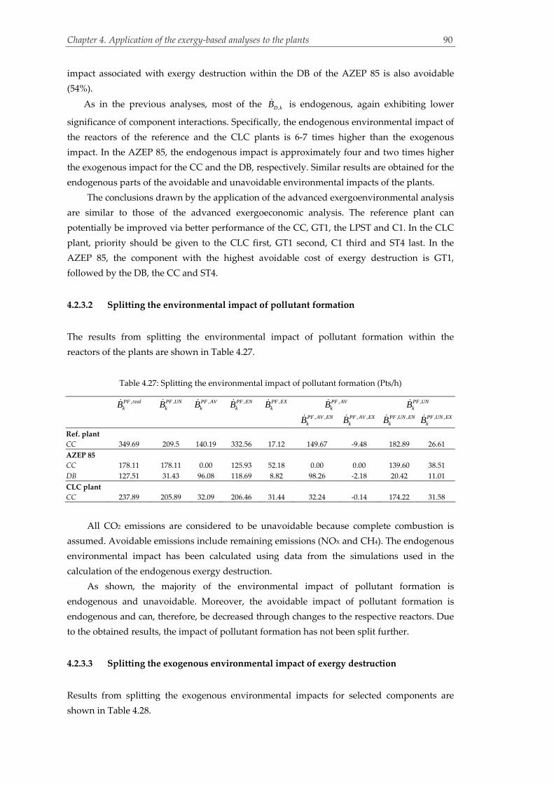
Chapter 4. Application of the exergy‐based analyses to the plants
90
impact associated with exergy destruction within the DB of the AZEP 85 is also avoidable
(54%).
As in the previous analyses, most of the ,
D kB is endogenous, again exhibiting lower
significance of component interactions. Specifically, the endogenous environmental impact of
the reactors of the reference and the CLC plants is 6‐7 times higher than the exogenous
impact. In the AZEP 85, the endogenous impact is approximately four and two times higher
the exogenous impact for the CC and the DB, respectively. Similar results are obtained for the
endogenous parts of the avoidable and unavoidable environmental impacts of the plants.
The conclusions drawn by the application of the advanced exergoenvironmental analysis
are similar to those of the advanced exergoeconomic analysis. The reference plant can
potentially be improved via better performance of the CC, GT1, the LPST and C1. In the CLC
plant, priority should be given to the CLC first, GT1 second, C1 third and ST4 last. In the
AZEP 85, the component with the highest avoidable cost of exergy destruction is GT1,
followed by the DB, the CC and ST4.
4.2.3.2 Splitting the environmental impact of pollutant formation
The results from splitting the environmental impact of pollutant formation within the
reactors of the plants are shown in Table 4.27.
Table 4.27: Splitting the environmental impact of pollutant formation (Pts/h)
,PF real
kB ,PF UNkB ,PF AV
kB ,PF EN
kB ,PF EXkB ,PF AV
kB ,PF UNkB
, ,PF AV EN
kB , ,PF AV EXkB , ,PF UN EN
kB , ,PF UN EXkB
Ref. plant
CC 349.69 209.5 140.19 332.56 17.12 149.67 ‐9.48 182.89 26.61
AZEP 85
CC 178.11 178.11 0.00 125.93 52.18 0.00 0.00 139.60 38.51
DB 127.51 31.43 96.08 118.69 8.82 98.26 ‐2.18 20.42 11.01
CLC plant
CC 237.89 205.89 32.09 206.46 31.44 32.24 ‐0.14 174.22 31.58
All CO2 emissions are considered to be unavoidable because complete combustion is
assumed. Avoidable emissions include remaining emissions (NOX and CH4). The endogenous
environmental impact has been calculated using data from the simulations used in the
calculation of the endogenous exergy destruction.
As shown, the majority of the environmental impact of pollutant formation is
endogenous and unavoidable. Moreover, the avoidable impact of pollutant formation is
endogenous and can, therefore, be decreased through changes to the respective reactors. Due
to the obtained results, the impact of pollutant formation has not been split further.
4.2.3.3 Splitting the exogenous environmental impact of exergy destruction
Results from splitting the exogenous environmental impacts for selected components are
shown in Table 4.28.
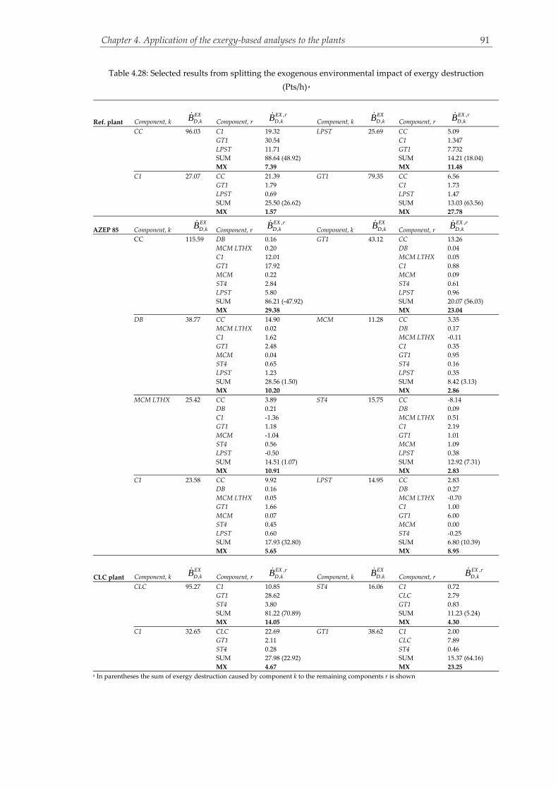
Chapter 4. Application of the exergy‐based analyses to the plants
91
Table 4.28: Selected results from splitting the exogenous environmental impact of exergy destruction
(Pts/h) a
Ref. plant Component, k , EX
D kB Component, r ,
, EX r
D kB Component, k , EX
D kB Component, r ,
, EX r
D kB
CC 96.03 C1 19.32 LPST 25.69 CC 5.09
GT1 30.54 C1 1.347
LPST 11.71 GT1 7.732
SUM 88.64 (48.92) SUM 14.21 (18.04)
MX 7.39 MX 11.48
C1 27.07 CC 21.39 GT1 79.35 CC 6.56
GT1 1.79 C1 1.73
LPST 0.69 LPST 1.47
SUM 25.50 (26.62) SUM 13.03 (63.56)
MX 1.57 MX 27.78
AZEP 85
Component, k , EX
D kB Component, r
,,
EX rD kB
Component, k , EX
D kB Component, r
,,
EX rD kB
CC 115.59 DB 0.16 GT1 43.12 CC 13.26
MCM LTHX 0.20 DB 0.04
C1 12.01 MCM LTHX 0.05
GT1 17.92 C1 0.88
MCM 0.22 MCM 0.09
ST4 2.84 ST4 0.61
LPST 5.80 LPST 0.96
SUM 86.21 (‐47.92) SUM 20.07 (56.03)
MX 29.38 MX 23.04
DB 38.77 CC 14.90 MCM 11.28 CC 3.35
MCM LTHX 0.02 DB 0.17
C1 1.62 MCM LTHX ‐0.11
GT1 2.48 C1 0.35
MCM 0.04 GT1 0.95
ST4 0.65 ST4 0.16
LPST 1.23 LPST 0.35
SUM 28.56 (1.50) SUM 8.42 (3.13)
MX 10.20 MX 2.86
MCM LTHX 25.42 CC 3.89 ST4 15.75 CC ‐8.14
DB 0.21 DB 0.09
C1 ‐1.36 MCM LTHX 0.51
GT1 1.18 C1 2.19
MCM ‐1.04 GT1 1.01
ST4 0.56 MCM 1.09
LPST ‐0.50 LPST 0.38
SUM 14.51 (1.07) SUM 12.92 (7.31)
MX 10.91 MX 2.83
C1 23.58 CC 9.92 LPST 14.95 CC 2.83
DB 0.16 DB 0.27
MCM LTHX 0.05 MCM LTHX ‐0.70
GT1 1.66 C1 1.00
MCM 0.07 GT1 6.00
ST4 0.45 MCM 0.00
LPST 0.60 ST4 ‐0.25
SUM 17.93 (32.80) SUM 6.80 (10.39)
MX 5.65 MX 8.95
CLC plant Component, k , EX
D kB Component, r ,
, EX r
D kB Component, k , EX
D kB Component, r ,
, EX r
D kB
CLC 95.27 C1 10.85 ST4 16.06 C1 0.72
GT1 28.62 CLC 2.79
ST4 3.80 GT1 0.83
SUM 81.22 (70.89) SUM 11.23 (5.24)
MX 14.05 MX 4.30
C1 32.65 CLC 22.69 GT1 38.62 C1 2.00
GT1 2.11 CLC 7.89
ST4 0.28 ST4 0.46
SUM 27.98 (22.92) SUM 15.37 (64.16)
MX 4.67 MX 23.25 a In parentheses the sum of exergy destruction caused by component k to the remaining components r is shown

Chapter 4. Application of the exergy‐based analyses to the plants
92
High values of the exogenous environmental impact are found for the reactors and the
components of the GT systems of the plants. A large part of the impact of the reactors is
caused by C1 and GT1: 52%, 41% and 26% of the impact imposed to the reactors stems from
GT1 and C1 in the reference plant, the CLC plant and the AZEP 85, respectively. This
percentage decreases to 11% for the DB of the AZEP 85. Analogously, large amounts of the
impact imposed on C1 and GT1 stem from the reactors.
Relatively high mexogenous values are found for GT1 in all of the plants, while the same
is true for the reactors of the oxy‐fuel plants with emphasis on the CC of the AZEP 85. In
general, the mexogenous values of the AZEP 85 are higher than those of the other plants
because of the more intense interactions of its constitutive components (e.g., a high
mexogenous value of the FG COND due to the large influence of the CC).
In summary, in the CLC plant, the highest exogenous environmental impact is caused by
the reactors, followed by GT1 and C1 (SUM, value in parentheses in Table 4.28). In the
reference plant, GT1 causes the highest impact, followed by the CC and C1. In the AZEP 85,
GT1 is followed by the MCM HTHX (35.2 Pts/h) and C1.
4.2.3.4 Calculating the total avoidable environmental impact of exergy destruction
The results of the most influential components of the plants are shown in Table 4.29. The total
avoidable exogenous environmental impact is calculated using Equation (3.38).
Table 4.29: Avoidable environmental impact of exergy destruction (Pts/h)
Ref. Plant
Component, k
, ,
,1
AV EX kn
D rrr k
B
,,
AV END kB
,,
AVD kB
CC 17.15 (7.4%) 215.01 (92.6%) 232.16
GT1 15.95 (27.2%) 42.77 (72.8) 58.72
C1 8.82 (31.5%) 19.17 (68.5%) 27.99
LPST 5.35 (22.6%) 18.30 (77.4%) 23.65
AZEP 85
Component, k
, ,
,1
AV EX kn
D rrr k
B
,,
AV END kB
,,
AVD kB
GT1 10.91 (24.8%) 33.15 (75.2%) 44.06
CC 1.24 (3.2%) 37.59 (96.8%) 38.83
DB ‐0.71 37.47 36.76
C1 5.73 (21.6%) 20.77 (78.4%) 26.50
LPST 4.53 (24.4%) 14.06 (75.6%) 18.59
MCM 3.33 (25.0%) 10.01 (75.0%) 13.34
MCM LTHX 0.39 (6.8%) 5.36 (93.2%) 5.75
CLC Plant
Component, k
, ,
,1
AV EX kn
D rrr k
B
,,
AV END kB
,,
AVD kB
CLC 20.48 (9.4%) 197.48 (90.6%) 217.96
GT1 16.93 (30.4%) 38.70 (69.6%) 55.63
C1 1.31 (5.8%) 21.27 (94.2%) 22.58
ST4 1.34 (7.5%) 16.60 (92.5%) 17.94
In the reference plant, GT1 causes an avoidable exogenous environmental impact similar
to that caused by the CC. However, the endogenous impact of the CC is approximately four

Chapter 4. Application of the exergy‐based analyses to the plants
93
times higher than that of GT1, resulting in a two times higher overall impact ( ,,
AVD kB ). In the
CLC plant, both the avoidable endogenous and exogenous values of the CLC reactor are
higher when compared to those of GT1, resulting in a higher overall impact, as well. In the
AZEP 85, the avoidable exogenous environmental impact of the DB is found to be negative,
while that of the CC is rather small. For the CC, this is a result of its negative influence on the
CO2 compression unit, while for the DB it is a result of the negative influence of the
component onto the MCM LTHX of the plant. Although the avoidable endogenous values of
the CC and DB are similar, the CC has a slightly higher avoidable impact due to its higher
avoidable exogenous part. The highest exogenous impact is caused by the MCM HTHX (19.9
Pts/h), followed by GT1 and C1. Again here, as in the case of the costs, the GT1 surpasses the
MCM HTHX in total impact, due to its relatively high avoidable endogenous part and it is
ranked first, followed by the CC and the DB.

Chapter 4. Application of the exergy‐based analyses to the plants
94
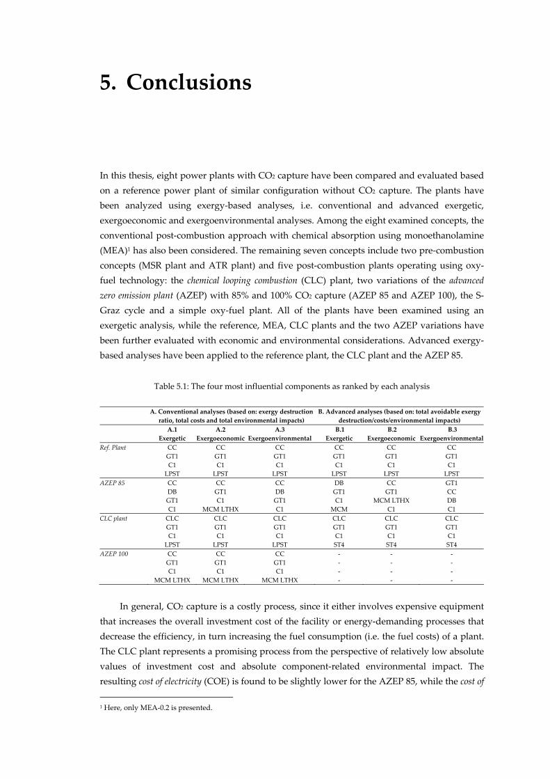
Chapter 5. Conclusions
95
5. Conclusions
In this thesis, eight power plants with CO2 capture have been compared and evaluated based
on a reference power plant of similar configuration without CO2 capture. The plants have
been analyzed using exergy‐based analyses, i.e. conventional and advanced exergetic,
exergoeconomic and exergoenvironmental analyses. Among the eight examined concepts, the
conventional post‐combustion approach with chemical absorption using monoethanolamine
(MEA)1 has also been considered. The remaining seven concepts include two pre‐combustion
concepts (MSR plant and ATR plant) and five post‐combustion plants operating using oxy‐
fuel technology: the chemical looping combustion (CLC) plant, two variations of the advanced
zero emission plant (AZEP) with 85% and 100% CO2 capture (AZEP 85 and AZEP 100), the S‐
Graz cycle and a simple oxy‐fuel plant. All of the plants have been examined using an
exergetic analysis, while the reference, MEA, CLC plants and the two AZEP variations have
been further evaluated with economic and environmental considerations. Advanced exergy‐
based analyses have been applied to the reference plant, the CLC plant and the AZEP 85.
Table 5.1: The four most influential components as ranked by each analysis
A. Conventional analyses (based on: exergy destruction
ratio, total costs and total environmental impacts)
B. Advanced analyses (based on: total avoidable exergy
destruction/costs/environmental impacts)
A.1
Exergetic
A.2
Exergoeconomic
A.3
Exergoenvironmental
B.1
Exergetic
B.2
Exergoeconomic
B.3
Exergoenvironmental
Ref. Plant CC CC CC CC CC CC
GT1 GT1 GT1 GT1 GT1 GT1
C1 C1 C1 C1 C1 C1
LPST LPST LPST LPST LPST LPST
AZEP 85 CC CC CC DB CC GT1
DB GT1 DB GT1 GT1 CC
GT1 C1 GT1 C1 MCM LTHX DB
C1 MCM LTHX C1 MCM C1 C1
CLC plant CLC CLC CLC CLC CLC CLC
GT1 GT1 GT1 GT1 GT1 GT1
C1 C1 C1 C1 C1 C1
LPST LPST LPST ST4 ST4 ST4
AZEP 100 CC CC CC ‐ ‐ ‐
GT1 GT1 GT1 ‐ ‐ ‐
C1 C1 C1 ‐ ‐ ‐
MCM LTHX MCM LTHX MCM LTHX ‐ ‐ ‐
In general, CO2 capture is a costly process, since it either involves expensive equipment
that increases the overall investment cost of the facility or energy‐demanding processes that
decrease the efficiency, in turn increasing the fuel consumption (i.e. the fuel costs) of a plant.
The CLC plant represents a promising process from the perspective of relatively low absolute
values of investment cost and absolute component‐related environmental impact. The
resulting cost of electricity (COE) is found to be slightly lower for the AZEP 85, while the cost of
1 Here, only MEA‐0.2 is presented.

Chapter 5. Conclusions
96
avoided CO2 (COA‐CO2) is lower for the CLC plant due to its higher amount of CO2 captured.
The environmental analysis shows that the efficiency decrease of the plants causes a
significant environmental burden. The oxy‐fuel plants show only minor reductions in the
overall impact compared to the reference plant. Furthermore, the conventional approach of
chemical absorption results in a higher environmental impact compared to the reference
plant, because of the high efficiency penalty associated with the technology used. Advanced
exergy‐based analyses have been used in order to pinpoint equipment and processes that
must be altered to improve the economic and environmental effectiveness of the overall
power plants.
As shown in Table 5.1, with the exception of the AZEP 85, the four most influential
components are the same in all conventional analyses. Although the DB of the AZEP 85 is
important from an exergetic perspective, it is relatively cheap and, therefore not so important
from an exergoeconomic point of view. The results of the advanced analyses associated with
the four most influential components of the reference and CLC plants, presented in Table 5.1,
agree with those of the conventional analyses with the exception of the ST4 in the CLC plant.
This is not the case when the AZEP 85 is considered, due to its more complicated
configuration and interactions of its components.
A short summary of the main results from each analysis is presented below.
5.1. Exergetic analysis
When compared to the reference plant that has an exergetic efficiency of 56.5%, the best
exergetic efficiency among all plants with CO2 capture was achieved by the AZEP 85 (53.4%),
followed by the AZEP 100 (51.7%) and the CLC plant (51.5%). The plant using chemical
absorption resulted in an efficiency penalty of eight percentage points (48.4%).
The three most efficient plants revealed in the exergetic analysis (AZEP 85, AZEP 100
and CLC plant) are oxy‐fuel concepts. Among the three plants, the CLC plant has the lowest
exergy destruction and the highest exergy loss (a result of the assumed 2% non‐reacted
methane). The combination of relatively low exergy destruction and loss (related to lower
mass flows of the exhausted gases) in the AZEP 85 results in higher net power output, i.e. a
higher exergetic efficiency. The main advantage of the three oxy‐fuel plants is that the added
components associated with CO2 capture do not consume high amounts of energy and the
energy penalties are mainly related to the production of oxygen necessary for the oxy‐
combustion. Moreover, the irreversibilities of the combustion processes in these plants are
lower compared with the reference and MEA plants, due to the nitrogen‐free combustion and
the preheating of the reactants used. The MEA plant results in a high efficiency penalty, due
to the relatively high energy requirements of chemical absorption.

Chapter 5. Conclusions
97
5.2. Economic analysis
The smallest cost increase, relative to the reference plant (total 213 € million), is estimated for
the MEA plant (total 326 € million), followed by the CLC plant (total 362 € million), the AZEP
85 (total 395 € million) and the AZEP 100 (total 414 € million).
Relative costs based on the power output of the plants present the MEA plant as the
most economical alternative (921 €/kW). However, if the cost is based on the amount of CO2
captured, the CLC plant is found to be more economical than the MEA plant because of its
approximately 100% CO2 capture (9.6 € million/kg CO2 captured versus 9.9 € million/kg CO2
captured for the MEA).
5.3. Exergoeconomic analysis
The cost of exergy destruction of the oxy‐fuel plants was found to be comparable to that of
the reference plant, while a larger difference was found for the MEA plant. Since all of the
plants have the same fuel cost rate ( Fc ), the total cost rate of exergy destruction ( ,D totC )
depends on the rate of exergy destruction ( ,D totE ; i.e., , ,D tot F D totC c E ). Thus, all differences
between exergy‐related cost rates are representative of the differences between the rates of
exergy destruction of the plants and that of the reference plant. Differences among the plants
mainly result from the high investment cost of components used for oxygen production
and/or facilitation of CO2 separation and compression.
CO2 capture causes a minimum increase in the cost of electricity of 22%, achieved by the
AZEP 85. An increase of 23% is calculated for the CLC plant, while the higher investment cost
of the AZEP 100 results in a more significant increase in the COE, similar to that of the MEA
(28% higher than that of the reference plant).
Larger differences in the energy penalty of the plants are observed when the COA‐CO2 is
considered. The cost differences between the MEA plant and the other plants are mainly
associated with the high energy demand of the solvent regeneration and the relatively low
percentage of CO2 capture (85%), in comparison to the close to 100% capture of the oxy‐fuel
concepts. The CLC plant has the same CO2 emissions as the AZEP 100, but it results in the
lowest COA‐CO2, due to its lower COE.
5.4. Life cycle assessment
The construction phase of the two AZEP concepts is associated with a significantly higher
environmental impact, with respect to the reference plant. The lowest relative component‐
related environmental impact (Pts/kW) among all plants with CO2 capture is found for the
CLC and MEA plants. However, the component‐related environmental impact of the plants is
negligible when compared to the impact associated with the exergy destruction that takes
place during the operation phase of the plants.

Chapter 5. Conclusions
98
5.5. Exergoenvironmental analysis
The calculation of the overall environmental impact is mainly influenced by the impacts of
fuel processing (methane) and the impact of pollutant emission. With data provided by
Goedkoop and Spriensma (2000), the impact of the produced electricity of the oxy‐fuel plants
is found to be slightly lower than that of the reference plant. Specifically, the CLC plant and
the AZEP 85 present the lowest environmental impact (0.6 Pts/MWh lower than that of the
reference plant). This marginal decrease in environmental impact raises questions concerning
the real environmental and cost viability of CO2 capture from power plants. Additionally, the
impact of the electricity generated in the MEA plant is found to be significantly higher than
that of the reference plant (2.4 Pts/MWh higher), due to the plant’s high efficiency penalty.
Considering that post‐combustion is the most conventional way to capture CO2 from power
plants, the plant has been considered in a sensitivity analysis concerning the variation of the
environmental impact of CO2 emissions. This analysis showed that post‐combustion
technology will not decrease the environmental impact of power production, unless a specific
environmental impact approximately four times higher than the present estimate is assigned
to the CO2 emissions.
5.6. Advanced exergetic analysis
Most of the exergy destruction of the plants is endogenous and, for the majority of the
components, unavoidable. Thus, improvement potential lies with the internal operating
conditions of the components (endogenous exergy destruction), while component interactions
(exogenous exergy destruction) are less significant. To examine the overall significance of the
different plant components, the total avoidable exergy destruction caused by each component
has been calculated. The total avoidable exergy destruction includes the exergy destruction
caused by each component both to itself and to the remaining components of the plant. The
results are similar to those of the conventional analysis: the improvement priority of the
reactors is ranked first, followed by GT1 and C1.
5.7. Advanced exergoeconomic analysis
In this analysis, the investment cost rate and the cost rate of exergy destruction are split into
avoidable/unavoidable and endogenous/exogenous parts. The improvement potential is
related to the avoidable part of the investment cost and the cost of exergy destruction. For the
reference and CLC plants, the most important components in terms of the absolute values of
the total avoidable costs are the reactors, GT1 and C1. In the AZEP 85, the ranking order
differs slightly when the total avoidable cost is considered, due to the large avoidable
investment cost of the MCM LTHX.
For the three most influential components of the plants, the largest part of their
investment cost rates and their cost of exergy destruction is unavoidable. Moreover, for both

Chapter 5. Conclusions
99
the investment cost and the cost of exergy destruction, the interactions of the components,
represented by the exogenous part of the costs, are of lower importance, since for the majority
of the components, the endogenous part of the costs is significantly larger.
5.8. Advanced exergoenvironmental analysis
The results of the advanced exergoenvironmental analysis generally agree with those
obtained in the other analyses. In general, the most important components are those of the GT
system, the LPST or ST4 and the MCM LTHX (in the case of the AZEP 85). A significantly
different result stems from the influence of the CC in the AZEP 85: The CC has an inverse
effect on the components processing the CO2 stream. Therefore, a low avoidable
environmental impact is caused by the CC, resulting in a small improvement priority of the
component (following that of GT1). On the contrary, in the other two plants, the reactors have
approximately four times higher total avoidable costs, when compared to GT1.
Similar to the results of the advanced exergoeconomic analysis, the majority of the
environmental impact related to the exergy destruction is unavoidable and endogenous.
Thus, the interactions of the components are of lower importance here as well.
5.9. Summary and future work
CO2 capture from power plants is a costly process. However, for CCS to be deemed viable,
the real economic and environmental benefits have to be considered. To do so, the
environmental perspective must be examined in detail, and different databases must be
compared and assessed. If it is decided that the obtained benefits represent realistic
expectations, the most cost effective solutions should be further promoted for large‐scale
implementation.
In general, oxy‐fuel concepts represent a relatively promising technology that keeps the
energy penalty of CO2 capture at relatively low levels, in contrast to the conventional
approach: chemical absorption with MEA.
The exergoeconomic and exergoenvironmental analyses provide important information
about how to improve both the structure and operating conditions of plants, in order to
decrease their economic penalty and increase their environmental advantage. Advanced
exergy‐based analyses are valuable supplements to the conventional analyses, providing
information about real improvement potential and component interactions. Nonetheless, the
analyses need to be further developed for more reliable process‐specific evaluation and easier
data processing.
Additionally, for a fair comparison of different power plants, various decision parameters
that may differ in importance from the point of view of technological availability, structure or
operation must be considered. Further research is essential, in order to find and evaluate
solutions which will avoid causing further environmental problems or creating additional
needs.

Chapter 5. Conclusions
100
Lastly, the information provided in this thesis should be used to realize improved
designs of the plant structures provided. This will provide a helpful guide on how
environmental and economic considerations interact and how optimized structures of the
plants can be obtained.

Appendix A. Flow charts and simulation assumptions of the power plants 101
Appendix A
Flow charts and simulation assumptions of
the power plants

Appendix A. Flow charts and simulation assumptions of the power plants 102
GG
M
M
M
M
M
7
63
12
5
Chi
mne
y
50 52
51
8
4
9
10
11
12
13
14
15
16
17
18
19
20
21 2
2
23
37
34
35
25
24
32
36
31
43
30
29
42
41
27
28
40
26
33
38
39
40
44
45
46
47
48
49
53
54
55
56
57
C1
GT1
CC
HP
ST
IPS
TLP
ST
CO
ND
COND
P LPEV
LPEC
LPS
H
IPE
C
IPE
VIP
SH
HPEC
HPEV
HPS
HRH
LPP
HP
PIP
P
CT
P
CT
GEN
1G
EN2
De-
aera
tor
M3
M2
M1
η: 5
8.9%
, ε: 5
6.5%
Wne
t: 4
12.5
MW
A.1: The reference plant
Figure A.1.1: Structure of the reference plant

Appendix A. Flow charts and simulation assumptions of the power plants 103
Table A.1.1: Results of the year‐by‐year economic analysis for the reference plant
Ref. Plant
Debt Book Adjustment Common Equity Book Adjustment TCR
Year Calendar year beg. of year depreciation beg. of year depreciation
1 2013 145,843,425 7,292,171 461,985 145,843,425 5,027,429 1,102,609 13,884,195
2 2014 138,089,269 7,292,171 461,985 139,713,386 5,027,429 1,102,609 13,884,195
3 2015 130,335,112 7,292,171 461,985 133,583,348 5,027,429 1,102,609 13,884,195
4 2016 122,580,956 7,292,171 461,985 127,453,309 5,027,429 1,102,609 13,884,195
5 2017 114,826,800 7,292,171 461,985 121,323,271 5,027,429 1,102,609 13,884,195
6 2018 107,072,644 7,292,171 461,985 115,193,232 5,027,429 1,102,609 13,884,195
7 2019 99,318,487 7,292,171 461,985 109,063,194 5,027,429 1,102,609 13,884,195
8 2020 91,564,331 7,292,171 461,985 102,933,155 5,027,429 1,102,609 13,884,195
9 2021 83,810,175 7,292,171 461,985 96,803,117 5,027,429 1,102,609 13,884,195
10 2022 76,056,018 7,292,171 461,985 90,673,078 5,027,429 1,102,609 13,884,195
11 2023 68,301,862 7,292,171 461,985 84,543,040 5,027,429 1,102,609 13,884,195
12 2024 60,547,706 7,292,171 461,985 78,413,001 5,027,429 1,102,609 13,884,195
13 2025 52,793,550 7,292,171 461,985 72,282,963 5,027,429 1,102,609 13,884,195
14 2026 45,039,393 7,292,171 461,985 66,152,924 5,027,429 1,102,609 13,884,195
15 2027 37,285,237 7,292,171 461,985 60,022,886 5,027,429 1,102,609 13,884,195
16 2028 29,531,081 7,292,171 461,985 53,892,847 5,027,429 1,102,609 13,884,195
17 2029 21,776,925 7,292,171 ‐1,847,940 47,762,809 5,027,429 ‐1,207,316 9,264,345
18 2030 16,332,694 7,292,171 ‐1,847,940 43,942,695 5,027,429 ‐1,207,316 9,264,345
19 2031 10,888,462 7,292,171 ‐1,847,940 40,122,582 5,027,429 ‐1,207,316 9,264,345
20 2032 5,444,231 7,292,171 ‐1,847,940 36,302,469 5,027,429 ‐1,207,316 9,264,345
21 2033 0 0 0 32,482,355 0 0 0
Total 1,457,438,358 145,843,425 0 1,798,503,086 100,548,585 12,812,485 259,204,494

Appendix A. Flow charts and simulation assumptions of the power plants 104
Table A.1.2: Results at the component level for the reference plant
,F kE ,P kE ,D kE k ,D ky ,F kc ,P kc ,D kC kZ ,D k kC Z kf kr ,F kb ,P kb ,D kB kY ,D k kB Y
,b kf ,b kr
Component, k (MW) (MW) (MW) (%) (%) (€/GJ) (€/GJ) (€/h) (€/h) (€/h) (%) (%) (Pts/GJ) (Pts/GJ) (Pts/h) (Pts/h) (Pts/h) (%) (%)
C1 242.68 231.30 11.38 95.3 1.56 16.9 19.5 693 1,423 2,116 67.3 15.0 6.1 6.4 249.71 0.24 249.94 0.09 4.9
CC 729.62 508.76 220.87 69.7 30.23 9.2 13.7 7,276 1,017 8,293 12.3 49.5 3.5 5.6 2746.20 0.38 2746.58 0.01 63.3
GT 551.15 530.67 20.47 96.3 2.80 15.5 16.9 1,140 1,627 2,766 58.8 9.4 5.9 6.1 432.58 1.12 433.71 0.26 3.9
HPSH 35.07 31.72 3.35 90.5 0.46 15.5 19.4 186 158 344 45.8 25.6 5.9 6.8 70.75 1.20 71.95 1.67 15.5
HPEV 43.64 39.91 3.73 91.5 0.51 15.5 19.0 207 185 392 47.1 23.1 5.9 6.7 78.75 0.13 78.88 0.16 13.6
HPEC 28.92 24.91 4.00 86.2 0.55 15.5 20.4 223 89 312 28.6 31.8 5.9 7.2 84.57 0.09 84.66 0.10 23.3
RH 26.47 23.89 2.58 90.3 0.35 15.5 19.4 143 111 255 43.7 25.4 5.9 6.8 54.42 0.80 55.22 1.46 15.8
IPSH 0.18 0.12 0.06 69.0 0.01 15.5 35.4 3 4 7 56.3 128.8 5.9 9.7 1.17 0.00 1.17 0.18 65.2
IPEV 6.10 5.67 0.43 92.9 0.06 15.5 20.5 24 65 90 73.1 32.8 5.9 6.5 9.13 0.04 9.16 0.42 11.1
IPEC 1.06 0.87 0.19 82.5 0.03 15.5 22.3 10 5 16 33.4 44.3 5.9 7.7 3.93 0.00 3.93 0.09 30.9
LPSH 1.43 1.04 0.38 73.3 0.05 15.5 29.5 21 19 41 47.7 90.9 5.9 9.0 8.05 0.01 8.06 0.16 53.0
LPEV 19.03 15.48 3.55 81.4 0.49 15.5 24.2 197 174 372 46.9 56.4 5.9 7.8 74.95 0.12 75.07 0.16 33.3
LPEC 11.49 7.71 3.78 67.1 0.52 15.5 30.8 211 93 304 30.7 99.3 5.9 10.1 79.97 0.09 80.07 0.12 71.3
HPST 31.29 29.18 2.11 93.2 0.29 20.3 24.2 155 182 336 54.0 18.9 7.0 7.7 53.51 0.28 53.79 0.51 10.0
IPST 37.39 35.21 2.18 94.2 0.30 20.3 24.7 159 329 488 67.4 21.7 7.0 7.6 54.88 0.32 55.20 0.57 8.6
LPST 70.99 61.35 9.64 86.4 1.32 21.4 29.7 743 764 1,508 50.7 38.5 7.2 8.8 251.49 0.49 251.98 0.20 21.5
COND P 0.04 0.04 0.01 78.8 0.00 20.0 84.2 1 7 8 91.3 321.6 6.7 9.3 0.23 0.00 0.23 0.13 37.5
HPP 1.12 0.96 0.17 85.3 0.02 20.0 36.7 12 40 52 77.3 83.8 6.7 8.4 4.00 0.00 4.00 0.01 24.0
IPP 0.03 0.02 0.01 65.3 0.00 20.0 147.4 1 8 8 91.4 637.6 6.7 11.7 0.25 0.00 0.25 0.01 73.8
LPP 0.00 0.00 0.00 67.2 0.00 20.0 406.5 0 3 3 97.4 1934.8 6.7 11.3 0.02 0.00 0.02 0.50 68.2
De‐aerator 0.56 0.53 0.03 95.4 0.00 25.1 41.2 2 28 30 92.4 64.3 8.1 8.6 0.74 0.04 0.77 4.55 6.6
M1 1.81 1.63 0.18 90.1 0.02 20.3 22.8 13 0 13 0.0 12.2 7.0 7.8 4.52 0.00 4.52 0.00 12.1
M2 0.63 0.58 0.04 92.9 0.01 20.3 24.7 3 0 3 0.0 21.3 7.0 8.4 1.12 0.00 1.12 0.00 19.2
M3 0.18 0.18 0.00 99.9 0.00 15.5 15.5 0 0 0 0.0 0.1 5.9 5.9 0.00 0.00 0.00 0.00 0.1
COND 12.43 ‐ 9.24 ‐ 1.26 21.4 ‐ 712 91 803 11.3 ‐ 7.2 ‐ 241.02 0.03 241.05 0.01 ‐
CT 3.19 ‐ 2.04 ‐ 0.28 ‐ ‐ ‐ 96 ‐ ‐ ‐ ‐ ‐ ‐ 11.95 ‐ ‐ ‐
Total 730.58 412.54 300.41 56.5 41.12 9.2 20.6 9,897 6,519 16,416 39.7 124.8 3.5 7.0 3735.22 17.33 3752.54 0.46 101.7
Exergy loss 17.63 PFkB 1258.87
Appen
dix A. Flow charts an
d simulation
assumption
s of the power plan
ts
104
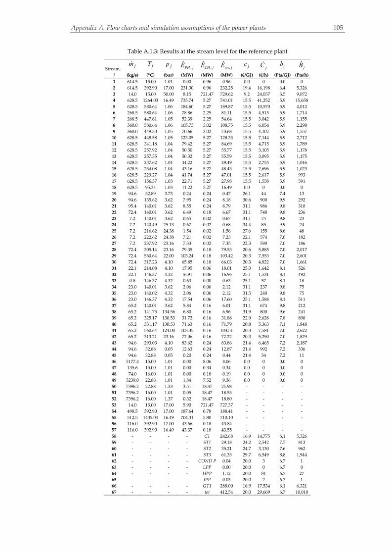
Appendix A. Flow charts and simulation assumptions of the power plants 105
Table A.1.3: Results at the stream level for the reference plant
Stream, jm jT jp
,PH jE ,CH jE ,tot jE jc jС jb
jB
j (kg/s) (°C) (bar) (MW) (MW) (MW) (€/GJ) (€/h) (Pts/GJ) (Pts/h)
1 614.5 15.00 1.01 0.00 0.96 0.96 0.0 0 0.0 0
2 614.5 392.90 17.00 231.30 0.96 232.25 19.4 16,198 6.4 5,326
3 14.0 15.00 50.00 8.15 721.47 729.62 9.2 24,037 3.5 9,072
4 628.5 1264.03 16.49 735.74 5.27 741.01 15.5 41,252 5.9 15,658
5 628.5 580.64 1.06 184.60 5.27 189.87 15.5 10,570 5.9 4,012
6 268.5 580.64 1.06 78.86 2.25 81.11 15.5 4,515 5.9 1,714
7 268.5 447.61 1.05 52.39 2.25 54.64 15.5 3,042 5.9 1,155
8 360.0 580.64 1.06 105.73 3.02 108.75 15.5 6,054 5.9 2,298
9 360.0 449.30 1.05 70.66 3.02 73.68 15.5 4,102 5.9 1,557
10 628.5 448.58 1.05 123.05 5.27 128.33 15.5 7,144 5.9 2,712
11 628.5 341.18 1.04 79.42 5.27 84.69 15.5 4,715 5.9 1,789
12 628.5 257.92 1.04 50.50 5.27 55.77 15.5 3,105 5.9 1,178
13 628.5 257.35 1.04 50.32 5.27 55.59 15.5 3,095 5.9 1,175
14 628.5 237.62 1.04 44.22 5.27 49.49 15.5 2,755 5.9 1,046
15 628.5 234.08 1.04 43.16 5.27 48.43 15.5 2,696 5.9 1,023
16 628.5 229.27 1.04 41.74 5.27 47.01 15.5 2,617 5.9 993
17 628.5 156.37 1.03 22.71 5.27 27.98 15.5 1,558 5.9 591
18 628.5 95.34 1.03 11.22 5.27 16.49 0.0 0 0.0 0
19 94.6 32.89 3.73 0.24 0.24 0.47 26.1 44 7.4 13
20 94.6 135.62 3.62 7.95 0.24 8.18 30.6 900 9.9 292
21 95.4 140.01 3.62 8.55 0.24 8.79 31.1 986 9.8 310
22 72.4 140.01 3.62 6.49 0.18 6.67 31.1 748 9.8 236
23 7.2 140.01 3.62 0.65 0.02 0.67 31.1 75 9.8 23
24 7.2 140.49 25.13 0.67 0.02 0.68 34.4 85 9.9 24
25 7.2 216.62 24.38 1.54 0.02 1.56 27.6 155 8.6 48
26 7.2 222.62 24.38 7.21 0.02 7.23 22.1 574 7.0 182
27 7.2 237.92 23.16 7.33 0.02 7.35 22.3 590 7.0 186
28 72.4 305.14 23.16 79.35 0.18 79.53 20.6 5,885 7.0 2,017
29 72.4 560.64 22.00 103.24 0.18 103.42 20.3 7,553 7.0 2,601
30 72.4 317.23 4.10 65.85 0.18 66.03 20.3 4,822 7.0 1,661
31 22.1 214.08 4.10 17.95 0.06 18.01 25.3 1,642 8.1 526
32 22.1 146.37 4.32 16.91 0.06 16.96 25.1 1,531 8.1 492
33 0.8 146.37 4.32 0.63 0.00 0.63 25.1 57 8.1 18
34 23.0 140.01 3.62 2.06 0.06 2.12 31.1 237 9.8 75
35 23.0 140.02 4.32 2.06 0.06 2.12 31.5 240 9.8 75
36 23.0 146.37 4.32 17.54 0.06 17.60 25.1 1,588 8.1 511
37 65.2 140.01 3.62 5.84 0.16 6.01 31.1 674 9.8 212
38 65.2 141.75 134.56 6.80 0.16 6.96 31.9 800 9.6 241
39 65.2 325.17 130.53 31.72 0.16 31.88 22.9 2,628 7.8 890
40 65.2 331.17 130.53 71.63 0.16 71.79 20.8 5,363 7.1 1,848
41 65.2 560.64 124.00 103.35 0.16 103.51 20.3 7,581 7.0 2,622
42 65.2 313.21 23.16 72.06 0.16 72.22 20.3 5,290 7.0 1,829
43 94.6 293.03 4.10 83.62 0.24 83.86 21.4 6,465 7.2 2,187
44 94.6 32.88 0.05 12.63 0.24 12.87 21.4 992 7.2 336
45 94.6 32.88 0.05 0.20 0.24 0.44 21.4 34 7.2 11
46 5177.4 15.00 1.01 0.00 8.06 8.06 0.0 0 0.0 0
47 135.6 15.00 1.01 0.00 0.34 0.34 0.0 0 0.0 0
48 74.0 16.00 1.01 0.00 0.18 0.19 0.0 0 0.0 0
49 5239.0 22.88 1.01 1.84 7.52 9.36 0.0 0 0.0 0
50 7396.2 22.88 1.33 3.51 18.47 21.98 ‐ ‐ ‐ ‐
51 7396.2 16.00 1.01 0.05 18.47 18.53 ‐ ‐ ‐ ‐
52 7396.2 16.00 1.37 0.32 18.47 18.80 ‐ ‐ ‐ ‐
53 14.0 15.00 17.00 5.90 721.47 727.37 ‐ ‐ ‐ ‐
54 498.5 392.90 17.00 187.64 0.78 188.41 ‐ ‐ ‐ ‐
55 512.5 1435.04 16.49 704.31 5.80 710.10 ‐ ‐ ‐ ‐
56 116.0 392.90 17.00 43.66 0.18 43.84 ‐ ‐ ‐ ‐
57 116.0 392.90 16.49 43.37 0.18 43.55 ‐ ‐ ‐ ‐
58 ‐ ‐ ‐ ‐ C1 242.68 16.9 14,775 6.1 5,326
59 ‐ ‐ ‐ ‐ ST1 29.18 24.2 2,542 7.7 813
60 ‐ ‐ ‐ ‐ ST2 35.21 24.7 3,130 7.6 962
61 ‐ ‐ ‐ ‐ ST3 61.35 29.7 6,549 8.8 1,944
62 ‐ ‐ ‐ ‐ COND P 0.04 20.0 3 6.7 1
63 ‐ ‐ ‐ ‐ LPP 0.00 20.0 0 6.7 0
64 ‐ ‐ ‐ ‐ HPP 1.12 20.0 81 6.7 27
65 ‐ ‐ ‐ ‐ IPP 0.03 20.0 2 6.7 1
66 ‐ ‐ ‐ ‐ GT1 288.00 16.9 17,534 6.1 6,321
67 ‐ ‐ ‐ ‐ tot 412.54 20.0 29,669 6.7 10,010

Appendix A. Flow charts and simulation assumptions of the power plants 106
Table A.1.4: Splitting the exergy destruction in the reference plant (MW)
Component,
k ,realD kE ,
END kE ,
EXD kE ,
AVD kE ,
UND kE ,
,UN END kE ,
,UN EXD kE ,
,AV END kE ,
,AV EXD kE
C1 11.38 6.94 4.44 5.11 6.26 3.79 2.47 3.14 1.97
CC 220.87 193.06 27.80 71.03 149.84 130.81 19.03 62.25 8.77
GT 16.09 13.52 2.57 8.32 7.77 6.23 1.53 7.29 1.03
HPSH 3.35 1.78 1.57 0.87 2.48 1.30 1.18 0.48 0.38
HPEV 3.73 2.00 1.72 0.67 3.06 1.84 1.21 0.16 0.51
HPEC 4.00 2.24 1.76 1.28 2.72 1.75 0.97 0.49 0.79
RH 2.57 1.98 0.59 0.89 1.68 1.11 0.57 0.87 0.02
IPSH 0.06 0.09 ‐0.03 0.05 0.01 0.01 ‐0.01 0.07 ‐0.03
IPEV 0.43 0.41 0.02 0.15 0.28 0.25 0.03 0.16 ‐0.01
IPEC 0.19 0.16 0.03 0.07 0.12 0.18 ‐0.06 ‐0.01 0.08
LPSH 0.38 0.19 0.19 0.22 0.16 0.06 0.10 0.13 0.09
LPEV 3.74 1.68 2.06 0.76 2.98 1.65 1.33 0.03 0.73
LPEC 3.78 2.42 1.37 1.83 1.95 1.13 0.82 1.28 0.55
HPST 1.67 1.11 0.56 0.89 0.78 0.50 0.29 0.61 0.28
IPST 1.65 1.19 0.46 0.71 0.94 0.65 0.28 0.54 0.17
LPST 8.71 6.10 2.61 3.61 5.10 3.57 1.53 2.53 1.08
COND P 0.45 0.00 0.44 0.45 0.00 0.00 0.00 0.00 0.44
HPP 0.11 0.00 0.11 0.11 0.00 0.00 0.00 0.00 0.11
IPP 0.01 0.06 ‐0.06 ‐0.03 0.03 0.02 0.01 0.04 ‐0.07
LPP 0.03 0.01 0.02 0.02 0.00 0.00 0.00 0.01 0.02
COND 9.24 6.49 2.75 ‐ ‐ ‐ ‐ ‐ ‐
CT 2.04 1.30 0.74 ‐ ‐ ‐ ‐ ‐ ‐
GEN1 4.39 4.76 ‐0.38 2.94 1.45 1.57 ‐0.12 3.19 ‐0.25
GEN2 1.91 1.44 0.48 1.28 0.63 0.47 0.16 0.96 0.32
MOT1 0.01 0.00 0.01 0.00 0.00 0.00 0.00 0.00 0.01
MOT2 0.15 0.00 0.15 0.15 0.00 0.00 0.00 0.00 0.15
MOT3 0.06 0.00 0.06 0.04 0.02 0.01 0.01 ‐0.01 0.05
MOT4 0.00 0.00 0.00 0.00 0.00 0.00 0.00 0.00 0.00
Total 300.97 248.94 52.03
Total (%) 82.71 17.29
Table A.1.5: Splitting the investment cost rate in the reference plant (€/h)
AVkZ
UNkZ
Component, k realkZ
UNkZ
AVkZ
ENkZ
EXkZ
,AV ENkZ
,AV EXkZ
,UN ENkZ
,UN EXkZ
C1 1423.3 1209.8 213.5 861.8 561.5 129.3 84.2 732.6 477.3
CC 1016.7 813.3 203.3 887.6 129.1 177.5 25.8 710.0 103.3
GT 1626.7 1464.0 162.7 1305.7 320.9 130.6 32.1 1175.2 288.8
HPSH 111.2 50.8 60.4 73.5 37.7 39.9 20.5 33.6 17.2
HPEV 157.7 68.5 89.2 82.4 75.2 46.6 42.6 35.8 32.7
HPEC 185.0 102.6 82.4 111.7 73.4 49.7 32.7 61.9 40.7
RH 89.2 45.2 44.1 57.3 31.9 28.4 15.7 29.0 16.3
IPSH 4.0 1.2 2.8 7.1 ‐3.1 5.0 ‐2.2 2.1 ‐0.9
IPEV 65.5 31.5 33.9 58.2 7.2 30.2 3.7 28.1 3.5
IPEC 5.2 2.8 2.4 7.6 ‐2.4 3.5 ‐1.1 4.1 ‐1.3
LPSH 19.3 7.6 11.7 7.7 11.6 4.7 7.0 3.1 4.6
LPEV 174.2 89.2 85.0 96.5 77.7 47.1 37.9 49.4 39.8
LPEC 93.4 44.9 48.5 54.2 39.2 28.1 20.4 26.1 18.9
HPST 181.7 163.5 18.2 115.3 66.4 11.5 6.6 103.8 59.7
IPST 328.9 296.0 32.9 230.1 98.8 23.0 9.9 207.1 89.0
LPST 764.1 687.7 76.4 534.9 229.2 53.5 22.9 481.4 206.3
COND P 7.1 6.1 1.1 5.6 1.5 0.8 0.2 4.8 1.3
HPP 40.5 34.4 6.1 23.9 16.6 3.6 2.5 20.3 14.1
IPP 7.8 6.6 1.2 9.8 ‐2.1 1.5 ‐0.3 8.4 ‐1.8
LPP 2.5 2.1 0.4 0.0 2.5 0.0 0.4 0.0 2.1

Appendix A. Flow charts and simulation assumptions of the power plants 107
Table A.1.6: Splitting the cost rate of exergy destruction in the reference plant (€/h)
,realD kC ,
UND kC ,
AVD kC
,END kC ,
EXD kC
,AVD kC
,UND kC
Component, k ,
,AV END kC
,,AV EXD kC
,
,UN END kC
,,UN EXD kC
C1 692.7 381.3 311.4 422.3 270.4 191.5 119.9 230.9 150.4
CC 7276.3 4936.4 2339.9 6360.4 916.0 2050.8 289.1 4309.5 626.9
GT 1139.7 432.3 707.4 752.7 387.0 405.6 301.7 347.0 85.3
HPSH 143.4 93.7 49.7 110.5 32.9 48.6 1.2 61.9 31.7
HPEV 186.4 138.2 48.2 99.2 87.2 27.0 21.2 72.3 65.9
HPEC 207.5 170.2 37.3 111.6 95.9 8.9 28.4 102.7 67.5
RH 222.8 151.4 71.4 124.8 98.1 27.5 43.9 97.2 54.2
IPSH 3.1 0.4 2.7 4.8 ‐1.7 4.1 ‐1.4 0.6 ‐0.3
IPEV 24.0 15.5 8.6 22.8 1.2 9.1 ‐0.5 13.7 1.7
IPEC 10.4 6.7 3.7 9.0 1.4 ‐0.8 4.5 9.8 ‐3.1
LPSH 21.2 8.9 12.3 10.8 10.4 7.2 5.1 3.6 5.3
LPEV 197.5 166.0 31.5 93.4 104.1 1.4 30.1 91.9 74.0
LPEC 210.7 108.8 101.9 134.6 76.1 71.5 30.4 63.1 45.7
HPST 154.7 57.3 97.4 81.0 73.7 44.6 52.8 36.4 20.9
IPST 159.3 68.3 91.0 86.9 72.5 39.1 51.9 47.8 20.5
LPST 743.4 393.2 350.2 470.0 273.4 194.7 155.5 275.3 117.9
COND P 0.7 0.1 0.6 0.2 0.5 0.1 0.4 0.1 0.0
HPP 11.9 2.5 9.4 4.5 7.4 3.0 6.4 1.5 1.0
IPP 0.7 0.0 0.7 0.6 0.2 0.5 0.2 0.1 0.0
LPP 0.1 0.0 0.1 0.0 0.1 0.0 0.1 0.0 0.0
Table A.1.7: Splitting the environmental impact of exergy destruction in the reference plant (Pts/h)
, realD kB ,
UND kB ,
AVD kB
, END kB ,
EXD kB
, AVD kB
,UND kB
Component, k ,
, AV END kB
,,
AV EXD kB
,
,UN END kB
,,
UN EXD kB
C1 69.4 38.2 31.2 42.3 27.1 19.2 12.0 23.1 15.1
CC 762.8 517.5 245.3 666.8 96.0 215.0 30.3 451.8 65.7
GT 120.2 45.6 74.6 79.4 40.8 42.8 31.8 36.6 9.0
HPSH 15.1 9.9 5.2 11.6 3.5 5.1 0.1 6.5 3.3
HPEV 19.7 14.6 5.1 10.5 9.2 2.8 2.2 7.6 7.0
HPEC 21.9 17.9 3.9 11.8 10.1 0.9 3.0 10.8 7.1
RH 23.5 16.0 7.5 13.2 10.3 2.9 4.6 10.3 5.7
IPSH 0.3 0.0 0.3 0.5 ‐0.2 0.4 ‐0.1 0.1 0.0
IPEV 2.5 1.6 0.9 2.4 0.1 1.0 ‐0.1 1.4 0.2
IPEC 1.1 0.7 0.4 0.9 0.1 ‐0.1 0.5 1.0 ‐0.3
LPSH 2.2 0.9 1.3 1.1 1.1 0.8 0.5 0.4 0.6
LPEV 20.8 17.5 3.3 9.8 11.0 0.2 3.2 9.7 7.8
LPEC 22.2 11.5 10.7 14.2 8.0 7.5 3.2 6.7 4.8
HPST 14.9 5.5 9.4 7.8 7.1 4.3 5.1 3.5 2.0
IPST 15.2 6.5 8.7 8.3 6.9 3.7 5.0 4.6 2.0
LPST 69.9 37.0 32.9 44.2 25.7 18.3 14.6 25.9 11.1
COND P 0.1 0.0 0.1 0.0 0.0 0.0 0.0 0.0 0.0
HPP 1.1 0.2 0.9 0.4 0.7 0.3 0.6 0.1 0.1
IPP 0.1 0.0 0.1 0.1 0.0 0.0 0.0 0.0 0.0
LPP 0.0 0.0 0.0 0.0 0.0 0.0 0.0 0.0 0.0

Appendix A. Flow charts and simulation assumptions of the power plants 108
GG
M
M
M
M
M
G
6
5
1
7
2
Chi
mne
y
4
3
94
93
95 8
9
92
88
86
87
84
85
83
82
81
61
90
62
63
58
42
41
29
8
9
10 11 12
13
14
15
16
17
18
19
20
21
22
23
37
34
35
24
25
26
27
28
30
31
32
33
36
38
39
40
43
44
45
46
47
48
49
50 5
1
52
53
54
55
56
57
59
60
64
656
6
67
68
69
70
71
72
73
74
75
76
77
78
79
80
91
96
η: 5
5.7%
, ε: 5
3.4%
Wne
t: 38
9.9
MW
101
104
105
107
108
114
112
113
115
117
102
103
109
101
100
119
118
110
111
98
99
97
106
116
120
121
C1
GT1
RH
HPS
H
HPE
V
HPE
C
IPSH
HP
P
LPP
IPP
LPSH
LPEV
LPEC
CO
ND
P
CT
P
CO
ND
LPST
IPST
HPS
T
GEN
2
GEN
1
CT
GEN
3G
T2
DB
MC
M R
EA
CTO
R
SH II
EV II
EC II
FG C
ON
DC
OO
L1C
2C
3C
4C
5C
OO
L2C
OO
L3C
OO
L4
IPEV
IPEC
ST4
De-
aera
tor
NG
PH
M1
M2
M4
M3
M6
M5
A.2: The AZEP 85
Figure A.2.1: Structure of the AZEP 85 (for the MCM reactor see Figure A.4.1)

Appendix A. Flow charts and simulation assumptions of the power plants 109
Table A.2.1: Results of the economic analysis for the AZEP 85
Debt Book Adjustment Common Equity Book Adjustment TCR
Year Calendar year beg. of year depreciation beg. of year depreciation
1 2013 254,669,410 12,733,471 849,998 254,669,410 9,933,140 2,026,210 25,542,819
2 2014 241,085,942 12,733,471 849,998 242,710,060 9,933,140 2,026,210 25,542,819
3 2015 227,502,474 12,733,471 849,998 230,750,709 9,933,140 2,026,210 25,542,819
4 2016 213,919,005 12,733,471 849,998 218,791,358 9,933,140 2,026,210 25,542,819
5 2017 200,335,537 12,733,471 849,998 206,832,008 9,933,140 2,026,210 25,542,819
6 2018 186,752,068 12,733,471 849,998 194,872,657 9,933,140 2,026,210 25,542,819
7 2019 173,168,600 12,733,471 849,998 182,913,306 9,933,140 2,026,210 25,542,819
8 2020 159,585,131 12,733,471 849,998 170,953,956 9,933,140 2,026,210 25,542,819
9 2021 146,001,663 12,733,471 849,998 158,994,605 9,933,140 2,026,210 25,542,819
10 2022 132,418,195 12,733,471 849,998 147,035,254 9,933,140 2,026,210 25,542,819
11 2023 118,834,726 12,733,471 849,998 135,075,904 9,933,140 2,026,210 25,542,819
12 2024 105,251,258 12,733,471 849,998 123,116,553 9,933,140 2,026,210 25,542,819
13 2025 91,667,789 12,733,471 849,998 111,157,202 9,933,140 2,026,210 25,542,819
14 2026 78,084,321 12,733,471 849,998 99,197,852 9,933,140 2,026,210 25,542,819
15 2027 64,500,852 12,733,471 849,998 87,238,501 9,933,140 2,026,210 25,542,819
16 2028 50,917,384 12,733,471 849,998 75,279,150 9,933,140 2,026,210 25,542,819
17 2029 37,333,916 12,733,471 ‐3,399,992 63,319,800 9,933,140 ‐2,223,779 17,042,840
18 2030 28,000,437 12,733,471 ‐3,399,992 55,610,439 9,933,140 ‐2,223,779 17,042,840
19 2031 18,666,958 12,733,471 ‐3,399,992 47,901,077 9,933,140 ‐2,223,779 17,042,840
20 2032 9,333,479 12,733,471 ‐3,399,992 40,191,716 9,933,140 ‐2,223,779 17,042,840
21 2033 0 0 0 32,482,355 0 0 0
Total 2,538,029,145 254,669,410 0 2,879,093,873 198,662,808 23,524,248 476,856,466
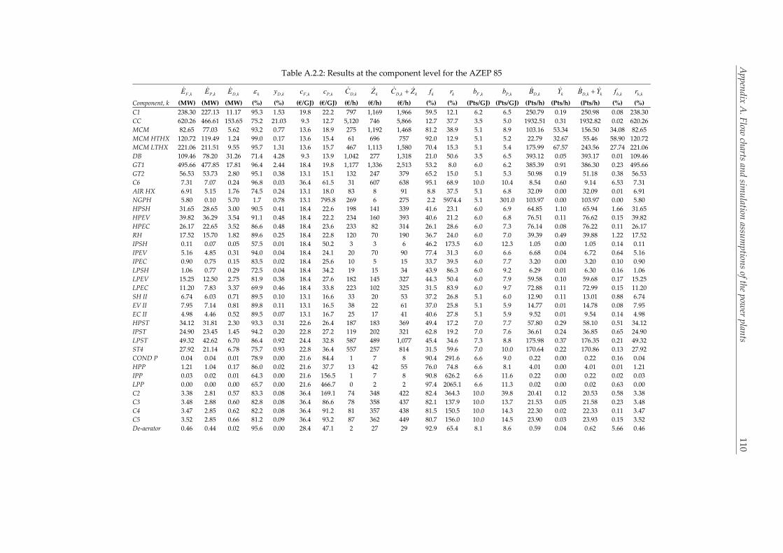
Appendix A. Flow charts and simulation assumptions of the power plants 110
Table A.2.2: Results at the component level for the AZEP 85
,F kE ,P kE ,D kE k ,D ky ,F kc ,P kc ,D kC kZ ,D k kC Z kf kr ,F kb ,P kb ,D kB kY ,D k kB Y
,b kf ,b kr
Component, k (MW) (MW) (MW) (%) (%) (€/GJ) (€/GJ) (€/h) (€/h) (€/h) (%) (%) (Pts/GJ) (Pts/GJ) (Pts/h) (Pts/h) (Pts/h) (%) (%)
C1 238.30 227.13 11.17 95.3 1.53 19.8 22.2 797 1,169 1,966 59.5 12.1 6.2 6.5 250.79 0.19 250.98 0.08 238.30
CC 620.26 466.61 153.65 75.2 21.03 9.3 12.7 5,120 746 5,866 12.7 37.7 3.5 5.0 1932.51 0.31 1932.82 0.02 620.26
MCM 82.65 77.03 5.62 93.2 0.77 13.6 18.9 275 1,192 1,468 81.2 38.9 5.1 8.9 103.16 53.34 156.50 34.08 82.65
MCM HTHX 120.72 119.49 1.24 99.0 0.17 13.6 15.4 61 696 757 92.0 12.9 5.1 5.2 22.79 32.67 55.46 58.90 120.72
MCM LTHX 221.06 211.51 9.55 95.7 1.31 13.6 15.7 467 1,113 1,580 70.4 15.3 5.1 5.4 175.99 67.57 243.56 27.74 221.06
DB 109.46 78.20 31.26 71.4 4.28 9.3 13.9 1,042 277 1,318 21.0 50.6 3.5 6.5 393.12 0.05 393.17 0.01 109.46
GT1 495.66 477.85 17.81 96.4 2.44 18.4 19.8 1,177 1,336 2,513 53.2 8.0 6.0 6.2 385.39 0.91 386.30 0.23 495.66
GT2 56.53 53.73 2.80 95.1 0.38 13.1 15.1 132 247 379 65.2 15.0 5.1 5.3 50.98 0.19 51.18 0.38 56.53
C6 7.31 7.07 0.24 96.8 0.03 36.4 61.5 31 607 638 95.1 68.9 10.0 10.4 8.54 0.60 9.14 6.53 7.31
AIR HX 6.91 5.15 1.76 74.5 0.24 13.1 18.0 83 8 91 8.8 37.5 5.1 6.8 32.09 0.00 32.09 0.01 6.91
NGPH 5.80 0.10 5.70 1.7 0.78 13.1 795.8 269 6 275 2.2 5974.4 5.1 301.0 103.97 0.00 103.97 0.00 5.80
HPSH 31.65 28.65 3.00 90.5 0.41 18.4 22.6 198 141 339 41.6 23.1 6.0 6.9 64.85 1.10 65.94 1.66 31.65
HPEV 39.82 36.29 3.54 91.1 0.48 18.4 22.2 234 160 393 40.6 21.2 6.0 6.8 76.51 0.11 76.62 0.15 39.82
HPEC 26.17 22.65 3.52 86.6 0.48 18.4 23.6 233 82 314 26.1 28.6 6.0 7.3 76.14 0.08 76.22 0.11 26.17
RH 17.52 15.70 1.82 89.6 0.25 18.4 22.8 120 70 190 36.7 24.0 6.0 7.0 39.39 0.49 39.88 1.22 17.52
IPSH 0.11 0.07 0.05 57.5 0.01 18.4 50.2 3 3 6 46.2 173.5 6.0 12.3 1.05 0.00 1.05 0.14 0.11
IPEV 5.16 4.85 0.31 94.0 0.04 18.4 24.1 20 70 90 77.4 31.3 6.0 6.6 6.68 0.04 6.72 0.64 5.16
IPEC 0.90 0.75 0.15 83.5 0.02 18.4 25.6 10 5 15 33.7 39.5 6.0 7.7 3.20 0.00 3.20 0.10 0.90
LPSH 1.06 0.77 0.29 72.5 0.04 18.4 34.2 19 15 34 43.9 86.3 6.0 9.2 6.29 0.01 6.30 0.16 1.06
LPEV 15.25 12.50 2.75 81.9 0.38 18.4 27.6 182 145 327 44.3 50.4 6.0 7.9 59.58 0.10 59.68 0.17 15.25
LPEC 11.20 7.83 3.37 69.9 0.46 18.4 33.8 223 102 325 31.5 83.9 6.0 9.7 72.88 0.11 72.99 0.15 11.20
SH II 6.74 6.03 0.71 89.5 0.10 13.1 16.6 33 20 53 37.2 26.8 5.1 6.0 12.90 0.11 13.01 0.88 6.74
EV II 7.95 7.14 0.81 89.8 0.11 13.1 16.5 38 22 61 37.0 25.8 5.1 5.9 14.77 0.01 14.78 0.08 7.95
EC II 4.98 4.46 0.52 89.5 0.07 13.1 16.7 25 17 41 40.6 27.8 5.1 5.9 9.52 0.01 9.54 0.14 4.98
HPST 34.12 31.81 2.30 93.3 0.31 22.6 26.4 187 183 369 49.4 17.2 7.0 7.7 57.80 0.29 58.10 0.51 34.12
IPST 24.90 23.45 1.45 94.2 0.20 22.8 27.2 119 202 321 62.8 19.2 7.0 7.6 36.61 0.24 36.85 0.65 24.90
LPST 49.32 42.62 6.70 86.4 0.92 24.4 32.8 587 489 1,077 45.4 34.6 7.3 8.8 175.98 0.37 176.35 0.21 49.32
ST4 27.92 21.14 6.78 75.7 0.93 22.8 36.4 557 257 814 31.5 59.6 7.0 10.0 170.64 0.22 170.86 0.13 27.92
COND P 0.04 0.04 0.01 78.9 0.00 21.6 84.4 1 7 8 90.4 291.6 6.6 9.0 0.22 0.00 0.22 0.16 0.04
HPP 1.21 1.04 0.17 86.0 0.02 21.6 37.7 13 42 55 76.0 74.8 6.6 8.1 4.01 0.00 4.01 0.01 1.21
IPP 0.03 0.02 0.01 64.3 0.00 21.6 156.5 1 7 8 90.8 626.2 6.6 11.6 0.22 0.00 0.22 0.02 0.03
LPP 0.00 0.00 0.00 65.7 0.00 21.6 466.7 0 2 2 97.4 2065.1 6.6 11.3 0.02 0.00 0.02 0.63 0.00
C2 3.38 2.81 0.57 83.3 0.08 36.4 169.1 74 348 422 82.4 364.3 10.0 39.8 20.41 0.12 20.53 0.58 3.38
C3 3.48 2.88 0.60 82.8 0.08 36.4 86.6 78 358 437 82.1 137.9 10.0 13.7 21.53 0.05 21.58 0.23 3.48
C4 3.47 2.85 0.62 82.2 0.08 36.4 91.2 81 357 438 81.5 150.5 10.0 14.3 22.30 0.02 22.33 0.11 3.47
C5 3.52 2.85 0.66 81.2 0.09 36.4 93.2 87 362 449 80.7 156.0 10.0 14.5 23.90 0.03 23.93 0.15 3.52
De‐aerator 0.46 0.44 0.02 95.6 0.00 28.4 47.1 2 27 29 92.9 65.4 8.1 8.6 0.59 0.04 0.62 5.66 0.46
Appen
dix A. Flow charts an
d simulation
assumption
s of the power plan
ts
110

Appendix A. Flow charts and simulation assumptions of the power plants 111
M1 1.43 1.28 0.15 89.5 0.02 22.8 26.5 12 0 12 0.0 16.4 7.0 8.1 3.78 0.00 3.78 0.00 1.43
M2 0.60 0.55 0.05 92.3 0.01 22.6 25.2 4 0 4 0.0 11.7 7.0 7.8 1.16 0.00 1.16 0.00 0.60
M3 1.70 1.69 0.01 99.1 0.00 18.4 18.6 1 0 1 0.0 1.3 6.0 6.1 0.31 0.00 0.31 0.00 1.70
M4 37.46 34.20 3.26 91.3 0.45 18.7 20.5 220 0 220 0.0 9.5 5.9 6.4 68.92 0.00 68.92 0.00 37.46
FG COND 15.09 ‐ 13.52 ‐ 1.85 13.2 ‐ 642 90 732 12.3 ‐ 5.1 ‐ 248.14 0.09 248.23 0.04 15.09
COOL1 0.68 ‐ 0.61 ‐ 0.08 46.3 ‐ 101 9 110 8.2 ‐ 12.5 ‐ 27.28 0.01 27.28 0.02 0.68
COOL2 0.81 ‐ 0.73 ‐ 0.10 53.8 ‐ 141 9 150 6.0 ‐ 12.7 ‐ 33.17 0.01 33.17 0.02 0.81
COOL3 0.76 ‐ 0.69 ‐ 0.09 59.9 ‐ 149 8 157 5.2 ‐ 12.9 ‐ 32.15 0.01 32.15 0.02 0.76
COOL4 0.79 ‐ 0.71 ‐ 0.10 64.7 ‐ 165 11 176 6.0 ‐ 13.2 ‐ 33.61 0.01 33.62 0.02 0.79
COND 12.29 ‐ 9.14 ‐ 1.25 23.9 ‐ 786 87 874 10.0 ‐ 7.2 ‐ 237.06 0.03 237.09 0.01 12.29
CT 4.92 ‐ 3.05 ‐ ‐ ‐ ‐ ‐ 93 ‐ ‐ ‐ ‐ ‐ ‐ 15.42 ‐ ‐ 4.92
Total 730.56 389.89 313.43 53.4 42.90 9.2 25.1 10,326 11,198 21,524 52.0 174.3 3.5 6.9 3897.09 174.95 4072.05 4.30 100.2
Exergy loss 27.25 PFkB CC 641.18 DB 459.05
Appen
dix A. Flow charts an
d simulation
assumption
s of the power plan
ts
111

Appendix A. Flow charts and simulation assumptions of the power plants 112
Table A.2.3: Results at the stream level for the AZEP 85
Stream, jm jT jp
,PH jE ,CH jE ,tot jE jc jС jb
jB
j (kg/s) (°C) (bar) (MW) (MW) (MW) (€/GJ) (€/h) (Pts/GJ) (Pts/h)
1 603.6 15.00 1.01 0.00 0.94 0.94 0.0 0 0.00 0
2 603.6 392.82 16.99 227.13 0.94 228.07 22.1 18,168 6.51 5,349
3 14.0 15.00 50.00 8.15 721.47 729.62 9.2 24,037 3.45 9,072
4 558.2 1301.93 16.81 649.44 1.43 650.87 18.4 43,005 6.01 14,082
5 558.2 578.70 1.06 153.78 1.43 155.21 18.4 10,255 6.01 3,358
6 218.2 578.70 1.06 60.11 0.56 60.67 18.4 4,009 6.01 1,313
7 218.2 466.96 1.05 42.59 0.56 43.15 18.4 2,851 6.01 934
8 340.0 578.70 1.06 93.67 0.87 94.54 18.4 6,246 6.01 2,045
9 340.0 447.82 1.05 62.02 0.87 62.89 18.4 4,155 6.01 1,361
10 558.2 455.31 1.05 104.60 1.43 106.03 18.4 7,007 6.01 2,294
11 558.2 341.18 1.04 64.78 1.43 66.21 18.4 4,375 6.01 1,433
12 558.2 252.75 1.04 38.61 1.43 40.03 18.4 2,646 6.01 866
13 558.2 252.34 1.04 38.49 1.43 39.92 18.4 2,638 6.01 864
14 558.2 232.62 1.04 33.33 1.43 34.76 18.4 2,297 6.01 752
15 558.2 229.08 1.04 32.43 1.43 33.86 18.4 2,238 6.01 733
16 558.2 224.88 1.04 31.38 1.43 32.80 18.4 2,168 6.01 710
17 558.2 156.37 1.03 16.13 1.43 17.55 18.4 1,160 6.01 380
18 558.2 84.65 1.03 4.92 1.43 6.35 0.0 0 0.00 0
19 95.0 32.89 3.73 0.24 0.24 0.48 28.4 49 7.34 13
20 95.0 136.37 3.62 8.07 0.24 8.31 33.5 1,001 9.53 285
21 95.7 140.01 3.62 8.58 0.24 8.82 34.1 1,082 9.47 300
22 77.1 140.01 3.62 6.91 0.19 7.11 34.1 873 9.47 242
23 6.2 140.01 3.62 0.55 0.02 0.57 34.1 70 9.47 19
24 6.2 140.50 25.13 0.57 0.02 0.59 37.6 79 9.53 20
25 6.2 216.62 24.38 1.32 0.02 1.34 30.9 148 8.49 41
26 6.2 222.62 24.38 6.18 0.02 6.19 25.6 570 6.97 155
27 6.2 232.75 23.16 6.24 0.02 6.26 25.8 581 7.03 158
28 77.1 307.14 23.16 84.69 0.19 84.88 22.8 6,971 6.99 2,135
29 48.4 558.70 22.00 68.78 0.12 68.91 22.8 5,656 6.99 1,734
30 48.4 315.74 4.10 43.88 0.12 44.00 22.8 3,612 6.99 1,107
31 17.9 209.08 4.10 14.40 0.04 14.45 28.7 1,495 8.13 423
32 17.9 146.37 4.32 13.64 0.04 13.68 28.4 1,401 8.07 398
33 0.7 146.37 4.32 0.52 0.00 0.53 28.4 54 8.07 15
34 18.5 140.01 3.62 1.66 0.05 1.71 34.1 210 9.47 58
35 18.5 140.02 4.32 1.66 0.05 1.71 34.5 212 9.47 58
36 18.5 146.37 4.32 14.16 0.05 14.21 28.4 1,455 8.07 413
37 71.0 140.01 3.62 6.36 0.18 6.54 34.1 803 9.47 223
38 71.0 141.72 134.56 7.40 0.18 7.57 34.6 943 9.28 253
39 59.3 325.17 130.53 28.83 0.15 28.98 26.0 2,714 7.75 809
40 59.3 331.17 130.53 65.12 0.15 65.27 23.9 5,620 7.24 1,702
41 71.0 561.95 124.00 112.61 0.18 112.79 22.6 9,158 6.98 2,833
42 71.0 314.23 23.16 78.50 0.18 78.67 22.6 6,388 6.98 1,976
43 66.2 286.89 4.10 58.13 0.17 58.30 24.4 5,112 7.30 1,532
44 66.2 32.88 0.05 8.81 0.17 8.98 24.4 787 7.30 236
45 95.0 32.88 0.05 0.20 0.24 0.44 23.9 38 7.21 11
46 6680.5 15.00 1.01 0.00 10.40 10.40 0.0 0 0.00 0
47 180.4 15.00 1.01 0.00 0.45 0.45 0.0 0 0.00 0
48 95.4 16.00 1.01 0.00 0.24 0.24 0.0 0 0.00 0
49 6765.5 23.60 1.01 2.88 9.72 12.60 0.0 0 0.00 0
50 48.4 307.14 23.16 53.09 0.12 53.21 22.8 4,370 6.99 1,338
51 28.8 307.14 23.16 31.60 0.07 31.68 22.8 2,601 6.99 797
52 28.8 32.88 0.05 3.68 0.07 3.75 22.8 308 6.99 94
53 95.0 32.88 0.05 12.49 0.24 12.73 23.9 1,095 7.21 330
54 59.3 141.72 134.56 6.18 0.15 6.33 34.6 788 9.28 211
55 11.7 141.72 134.56 1.22 0.03 1.25 34.6 155 9.28 42
56 11.7 325.17 130.53 5.67 0.03 5.70 20.6 424 6.67 137
57 11.7 331.17 130.53 12.82 0.03 12.85 18.3 848 6.25 289
58 11.7 578.56 124.00 18.85 0.03 18.87 17.8 1,208 6.16 418
59 59.3 558.70 124.00 93.77 0.15 93.92 23.5 7,950 7.14 2,415
60 59.4 1275.57 16.48 104.08 10.48 114.56 13.1 5,403 5.06 2,089
61 59.4 1200.00 16.47 97.17 10.48 107.65 13.1 5,077 5.06 1,963
62 59.4 684.07 1.04 40.64 10.48 51.12 13.1 2,411 5.06 932
63 59.4 598.56 1.04 34.84 10.48 45.32 13.1 2,137 5.06 826
64 59.4 490.15 1.04 28.10 10.48 38.58 13.1 1,820 5.06 703
65 59.4 341.18 1.03 20.15 10.48 30.63 13.1 1,445 5.06 558
66 59.4 222.27 1.02 15.17 10.48 25.65 13.1 1,210 5.06 468
67 33.6 30.00 1.01 0.04 10.42 10.45 13.1 493 5.06 191
68 25.7 30.00 1.01 0.04 0.06 0.10 0.0 0 0.00 0

Appendix A. Flow charts and simulation assumptions of the power plants 113
69 33.6 138.23 3.22 2.85 10.42 13.26 46.2 2,204 12.43 594
70 33.4 40.00 3.21 2.16 10.41 12.58 46.2 2,091 12.43 563
71 0.3 40.00 3.21 0.00 0.00 0.00 0.0 0 0.00 0
72 33.4 152.09 10.22 5.05 10.41 15.46 53.7 2,990 12.66 705
73 33.2 40.00 10.21 4.23 10.42 14.65 53.7 2,833 12.66 668
74 0.2 40.00 10.21 0.00 0.00 0.00 0.0 0 0.00 0
75 33.2 153.10 32.46 7.08 10.42 17.50 59.8 3,768 12.93 815
76 33.1 40.00 32.45 6.31 10.43 16.74 59.8 3,603 12.93 779
77 0.1 40.00 32.45 0.00 0.00 0.00 0.0 0 0.00 0
78 33.1 155.13 103.09 9.16 10.43 19.59 64.7 4,561 13.17 929
79 33.1 30.00 103.09 8.36 10.44 18.80 0.0 0 0.00 0
80 0.0 30.00 103.09 0.00 0.00 0.00 0.0 0 0.00 0
81 60.4 522.50 16.98 27.86 0.09 27.96 21.4 2,151 6.57 661
82 60.4 392.82 16.99 22.71 0.09 22.81 22.1 1,817 6.51 535
83 543.2 392.82 16.99 204.41 0.85 205.26 22.1 16,351 6.51 4,814
84 543.2 900.00 16.96 415.92 0.85 416.77 18.9 28,284 5.97 8,955
85 495.7 1000.00 17.00 427.27 1.21 428.48 19.7 30,325 6.05 9,328
86 354.5 1060.23 17.09 507.81 62.58 570.39 13.6 27,918 5.12 10,512
87 402.0 964.22 17.02 492.04 61.01 553.05 13.6 27,069 5.12 10,192
88 495.7 1250.00 16.98 546.76 1.21 547.97 18.7 36,930 5.87 11,586
89 402.0 487.78 16.99 270.99 61.01 331.99 13.6 16,249 5.12 6,118
90 413.9 1275.57 16.48 725.55 73.06 798.60 13.1 37,664 5.06 14,561
91 354.5 1275.57 16.48 621.47 62.58 684.04 13.1 32,261 5.06 12,472
92 354.5 1286.22 17.10 628.54 62.58 691.11 13.6 33,826 5.12 12,736
93 11.9 250.00 16.99 7.01 613.25 620.26 9.3 20,669 3.49 7,801
94 14.0 250.00 16.98 8.25 721.47 729.72 9.3 24,317 3.49 9,178
95 2.1 250.00 16.98 1.24 108.22 109.46 9.3 3,647 3.49 1,377
96 556.1 1174.45 16.98 571.44 1.23 572.67 19.0 39,081 5.94 12,246
97 7314.8 16.00 1.37 0.32 18.27 18.59 ‐ ‐ ‐ ‐
98 7314.8 22.88 1.33 3.47 18.27 21.74 ‐ ‐ ‐ ‐
99 9543.6 23.60 1.33 5.34 23.84 29.18 ‐ ‐ ‐ ‐
100 2228.9 26.00 1.33 1.98 5.57 7.55 ‐ ‐ ‐ ‐
101 2137.4 26.00 1.33 1.90 5.34 7.24 ‐ ‐ ‐ ‐
102 2051.4 26.00 1.33 1.82 5.12 6.95 ‐ ‐ ‐ ‐
103 1956.4 26.00 1.33 1.74 4.89 6.62 ‐ ‐ ‐ ‐
104 1867.6 26.00 1.33 1.66 4.67 6.32 ‐ ‐ ‐ ‐
105 1867.6 16.00 1.37 0.08 4.67 4.75 ‐ ‐ ‐ ‐
106 9182.4 16.00 1.37 0.40 22.94 23.33 ‐ ‐ ‐ ‐
107 9271.1 16.00 1.37 0.40 23.16 23.56 ‐ ‐ ‐ ‐
108 9366.2 16.00 1.37 0.41 23.40 23.80 ‐ ‐ ‐ ‐
109 9452.1 16.00 1.37 0.41 23.61 24.02 ‐ ‐ ‐ ‐
110 9543.6 16.00 1.01 0.07 23.84 23.91 ‐ ‐ ‐ ‐
111 9543.6 16.00 1.37 0.41 23.84 24.25 ‐ ‐ ‐ ‐
112 88.8 16.00 1.37 0.00 0.22 0.23 ‐ ‐ ‐ ‐
113 88.8 26.00 1.33 0.08 0.22 0.30 ‐ ‐ ‐ ‐
114 95.1 16.00 1.37 0.00 0.24 0.24 ‐ ‐ ‐ ‐
115 95.1 26.00 1.33 0.08 0.24 0.32 ‐ ‐ ‐ ‐
116 85.9 16.00 1.37 0.00 0.21 0.22 ‐ ‐ ‐ ‐
117 85.9 26.00 1.33 0.08 0.21 0.29 ‐ ‐ ‐ ‐
118 91.5 16.00 1.37 0.00 0.23 0.23 ‐ ‐ ‐ ‐
119 91.5 26.00 1.33 0.08 0.23 0.31 ‐ ‐ ‐ ‐
120 14.0 15.00 17.00 5.90 721.47 727.37 ‐ ‐ ‐ ‐
121 28.8 45.81 0.10 6.02 0.07 6.09 ‐ ‐ ‐ ‐
122 ‐ ‐ ‐ ‐ C1 238.30 19.8 16,999 6.23 5,349
123 ‐ ‐ ‐ ‐ ST1 31.81 26.4 3,027 7.66 878
124 ‐ ‐ ‐ ‐ ST2 23.45 27.2 2,293 7.58 640
125 ‐ ‐ ‐ ‐ ST3 42.62 32.8 5,032 8.83 1,356
126 ‐ ‐ ‐ ‐ COND P 0.04 21.6 3 6.59 1
127 ‐ ‐ ‐ ‐ LPP 0.00 21.6 0 6.59 0
128 ‐ ‐ ‐ ‐ HPP 1.21 21.6 94 6.59 29
129 ‐ ‐ ‐ ‐ IPP 0.03 21.6 2 6.59 1
130 ‐ ‐ ‐ ‐ GT1 239.55 19.8 17,088 6.23 5,377
131 ‐ ‐ ‐ ‐ GT2 53.73 15.1 2,913 5.33 1,031
132 ‐ ‐ ‐ ‐ C6 7.31 36.4 958 10.02 264
133 ‐ ‐ ‐ ‐ C2 3.38 36.4 443 10.02 122
134 ‐ ‐ ‐ ‐ C3 3.48 36.4 456 10.02 126
135 ‐ ‐ ‐ ‐ C4 3.47 36.4 454 10.02 125
136 ‐ ‐ ‐ ‐ C5 3.52 36.4 461 10.02 127
137 ‐ ‐ ‐ ‐ ST4 21.14 36.4 2,771 10.02 763
138 tot 389.89 21.6 30.2 6.59 9,250
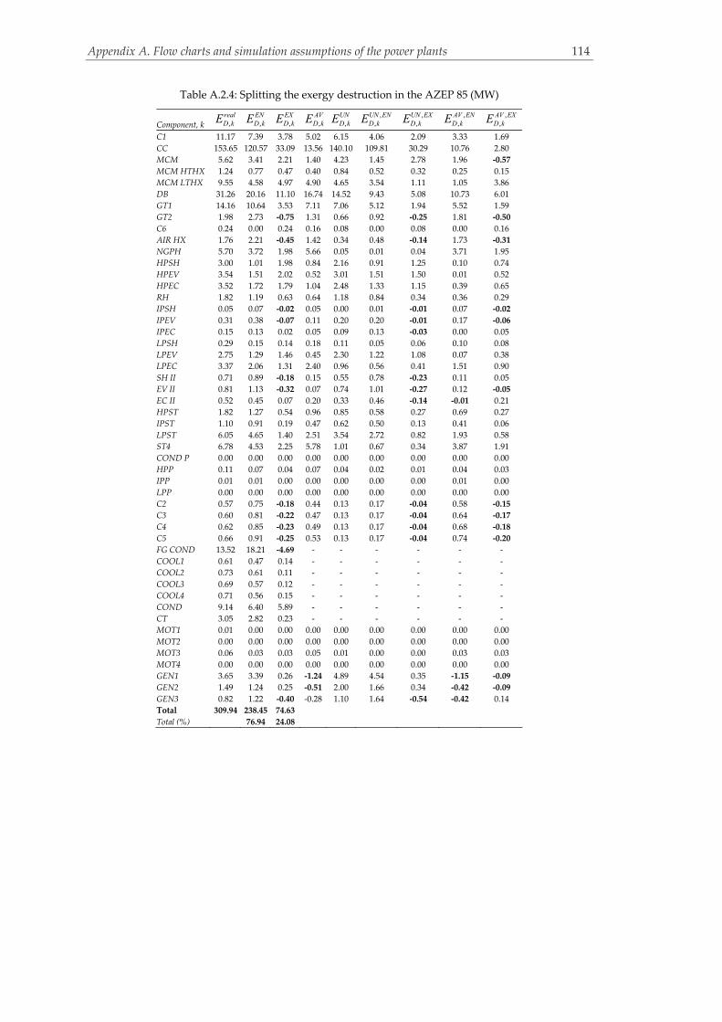
Appendix A. Flow charts and simulation assumptions of the power plants 114
Table A.2.4: Splitting the exergy destruction in the AZEP 85 (MW)
Component, k ,realD kE ,
END kE ,
EXD kE ,
AVD kE ,
UND kE ,
,UN END kE ,
,UN EXD kE ,
,AV END kE ,
,AV EXD kE
C1 11.17 7.39 3.78 5.02 6.15 4.06 2.09 3.33 1.69
CC 153.65 120.57 33.09 13.56 140.10 109.81 30.29 10.76 2.80
MCM 5.62 3.41 2.21 1.40 4.23 1.45 2.78 1.96 ‐0.57
MCM HTHX 1.24 0.77 0.47 0.40 0.84 0.52 0.32 0.25 0.15
MCM LTHX 9.55 4.58 4.97 4.90 4.65 3.54 1.11 1.05 3.86
DB 31.26 20.16 11.10 16.74 14.52 9.43 5.08 10.73 6.01
GT1 14.16 10.64 3.53 7.11 7.06 5.12 1.94 5.52 1.59
GT2 1.98 2.73 ‐0.75 1.31 0.66 0.92 ‐0.25 1.81 ‐0.50
C6 0.24 0.00 0.24 0.16 0.08 0.00 0.08 0.00 0.16
AIR HX 1.76 2.21 ‐0.45 1.42 0.34 0.48 ‐0.14 1.73 ‐0.31
NGPH 5.70 3.72 1.98 5.66 0.05 0.01 0.04 3.71 1.95
HPSH 3.00 1.01 1.98 0.84 2.16 0.91 1.25 0.10 0.74
HPEV 3.54 1.51 2.02 0.52 3.01 1.51 1.50 0.01 0.52
HPEC 3.52 1.72 1.79 1.04 2.48 1.33 1.15 0.39 0.65
RH 1.82 1.19 0.63 0.64 1.18 0.84 0.34 0.36 0.29
IPSH 0.05 0.07 ‐0.02 0.05 0.00 0.01 ‐0.01 0.07 ‐0.02
IPEV 0.31 0.38 ‐0.07 0.11 0.20 0.20 ‐0.01 0.17 ‐0.06
IPEC 0.15 0.13 0.02 0.05 0.09 0.13 ‐0.03 0.00 0.05
LPSH 0.29 0.15 0.14 0.18 0.11 0.05 0.06 0.10 0.08
LPEV 2.75 1.29 1.46 0.45 2.30 1.22 1.08 0.07 0.38
LPEC 3.37 2.06 1.31 2.40 0.96 0.56 0.41 1.51 0.90
SH II 0.71 0.89 ‐0.18 0.15 0.55 0.78 ‐0.23 0.11 0.05
EV II 0.81 1.13 ‐0.32 0.07 0.74 1.01 ‐0.27 0.12 ‐0.05
EC II 0.52 0.45 0.07 0.20 0.33 0.46 ‐0.14 ‐0.01 0.21
HPST 1.82 1.27 0.54 0.96 0.85 0.58 0.27 0.69 0.27
IPST 1.10 0.91 0.19 0.47 0.62 0.50 0.13 0.41 0.06
LPST 6.05 4.65 1.40 2.51 3.54 2.72 0.82 1.93 0.58
ST4 6.78 4.53 2.25 5.78 1.01 0.67 0.34 3.87 1.91
COND P 0.00 0.00 0.00 0.00 0.00 0.00 0.00 0.00 0.00
HPP 0.11 0.07 0.04 0.07 0.04 0.02 0.01 0.04 0.03
IPP 0.01 0.01 0.00 0.00 0.00 0.00 0.00 0.01 0.00
LPP 0.00 0.00 0.00 0.00 0.00 0.00 0.00 0.00 0.00
C2 0.57 0.75 ‐0.18 0.44 0.13 0.17 ‐0.04 0.58 ‐0.15
C3 0.60 0.81 ‐0.22 0.47 0.13 0.17 ‐0.04 0.64 ‐0.17
C4 0.62 0.85 ‐0.23 0.49 0.13 0.17 ‐0.04 0.68 ‐0.18
C5 0.66 0.91 ‐0.25 0.53 0.13 0.17 ‐0.04 0.74 ‐0.20
FG COND 13.52 18.21 ‐4.69 ‐ ‐ ‐ ‐ ‐ ‐
COOL1 0.61 0.47 0.14 ‐ ‐ ‐ ‐ ‐ ‐
COOL2 0.73 0.61 0.11 ‐ ‐ ‐ ‐ ‐ ‐
COOL3 0.69 0.57 0.12 ‐ ‐ ‐ ‐ ‐ ‐
COOL4 0.71 0.56 0.15 ‐ ‐ ‐ ‐ ‐ ‐
COND 9.14 6.40 5.89 ‐ ‐ ‐ ‐ ‐ ‐
CT 3.05 2.82 0.23 ‐ ‐ ‐ ‐ ‐ ‐
MOT1 0.01 0.00 0.00 0.00 0.00 0.00 0.00 0.00 0.00
MOT2 0.00 0.00 0.00 0.00 0.00 0.00 0.00 0.00 0.00
MOT3 0.06 0.03 0.03 0.05 0.01 0.00 0.00 0.03 0.03
MOT4 0.00 0.00 0.00 0.00 0.00 0.00 0.00 0.00 0.00
GEN1 3.65 3.39 0.26 ‐1.24 4.89 4.54 0.35 ‐1.15 ‐0.09
GEN2 1.49 1.24 0.25 ‐0.51 2.00 1.66 0.34 ‐0.42 ‐0.09
GEN3 0.82 1.22 ‐0.40 ‐0.28 1.10 1.64 ‐0.54 ‐0.42 0.14
Total 309.94 238.45 74.63
Total (%) 76.94 24.08

Appendix A. Flow charts and simulation assumptions of the power plants 115
Table A.2.5: Splitting the investment cost rate in the AZEP 85 (€/h)
AVkZ
UNkZ
Component, k realkZ
UNkZ
AVkZ
ENkZ
EXkZ
,AV ENkZ
,AV EXkZ
UNENkZ
,UN EXkZ
C1 1169.3 993.9 175.4 771.7 397.7 115.7 59.7 655.9 338.0
CC 745.9 596.7 149.2 584.6 161.3 116.9 32.3 467.7 129.0
MCM 1192.3 953.9 238.5 407.9 784.4 81.6 156.9 326.3 627.6
MCM HTHX 696.3 108.9 548.8 434.4 261.9 309.8 239.0 124.7 ‐15.8
MCM LTHX 1113.0 320.2 764.5 847.1 265.8 558.5 206.0 288.7 31.6
DB 276.8 221.5 55.4 179.9 96.9 36.0 19.4 143.9 77.5
GT1 1336.4 1202.8 133.6 970.0 366.4 97.0 36.6 873.0 329.8
GT2 247.3 222.5 24.7 341.1 ‐93.9 34.1 ‐9.4 307.0 ‐84.5
AIR HX 8.0 1.8 6.2 11.3 ‐3.3 8.7 ‐2.5 2.5 ‐0.7
NGPH 6.0 2.8 3.2 1.4 4.7 0.7 2.5 0.6 2.2
HPSH 141.3 58.6 82.6 59.7 81.6 34.9 47.7 24.8 33.9
HPEV 159.5 84.9 74.6 79.9 79.7 37.4 37.3 42.5 42.4
HPEC 81.9 39.3 42.6 44.0 37.9 22.9 19.7 21.1 18.2
RH 69.8 31.5 38.3 49.6 20.2 27.2 11.1 22.4 9.1
IPSH 2.7 0.7 2.0 8.0 ‐5.3 5.8 ‐3.8 2.2 ‐1.4
IPEV 69.9 25.6 44.3 72.5 ‐2.6 45.9 ‐1.6 26.6 ‐0.9
IPEC 5.0 2.3 2.7 6.8 ‐1.8 3.7 ‐1.0 3.1 ‐0.8
LPSH 15.1 5.6 9.4 6.3 8.8 3.9 5.5 2.3 3.3
LPEV 145.0 70.1 74.8 77.0 68.0 39.7 35.1 37.2 32.9
LPEC 102.5 44.1 58.4 59.0 43.5 33.6 24.8 25.4 18.7
SH II 19.7 8.8 11.0 27.9 ‐8.1 15.5 ‐4.5 12.4 ‐3.6
EV II 22.4 14.3 8.1 30.7 ‐8.3 11.1 ‐3.0 19.6 ‐5.3
EC II 16.8 7.3 9.6 23.8 ‐7.0 13.5 ‐4.0 10.3 ‐3.0
HPST 182.6 164.3 18.3 124.4 58.2 12.4 5.8 112.0 52.3
IPST 201.8 181.7 20.2 161.0 40.8 16.1 4.1 144.9 36.7
LPST 489.2 440.3 48.9 376.1 113.2 37.6 11.3 338.5 101.8
ST4 256.7 231.1 25.7 170.0 86.8 17.0 8.7 153.0 78.1
COND P 6.9 5.9 6.9 5.5 1.5 0.8 6.1 4.7 1.2
HPP 41.6 35.4 41.6 25.6 16.0 3.8 37.8 21.8 13.6
IPP 7.1 6.0 7.1 8.4 ‐1.3 1.3 5.8 7.1 ‐1.1
LPP 2.4 2.0 2.4 0.0 2.4 0.0 2.4 0.0 2.0
C2 347.9 295.7 52.2 448.8 ‐100.9 67.3 ‐15.1 381.5 ‐85.8
C3 358.4 304.6 53.8 479.9 ‐121.5 72.0 ‐18.2 407.9 ‐103.3
C4 356.9 303.3 53.5 480.3 ‐123.5 72.0 ‐18.5 408.3 ‐104.9
C5 362.1 307.8 54.3 488.2 ‐126.1 73.2 ‐18.9 415.0 ‐107.2
FG COND 90.4
COOL1 9.1
COOL2 9.0
COOL3 8.2
COOL4 10.6
COND 6.0

Appendix A. Flow charts and simulation assumptions of the power plants 116
Table A.2.6: Splitting the cost rate of exergy destruction in the AZEP 85 (€/h)
,realD kC ,
UND kC ,
AVD kC
,END kC ,
EXD kC
,AVD kC
,UND kC
Component, k ,
,AV END kC
,,AV EXD kC
,
,UN END kC
,,UN EXD kC
C1 797.1 438.8 358.3 527.2 269.8 237.7 120.6 289.6 149.2
CC 5120.2 4668.5 451.8 4017.7 1102.5 358.5 93.3 3659.2 1009.3
MCM 275.3 206.8 68.5 166.9 108.4 96.2 ‐27.7 70.8 136.1
MCM HTHX 60.5 41.0 19.5 37.6 22.9 12.0 7.5 25.6 15.4
MCM LTHX 467.4 227.5 239.9 224.4 243.0 51.2 188.7 173.2 54.3
DB 1041.6 483.8 557.8 671.8 369.8 357.4 200.4 314.4 169.4
GT1 1176.9 466.3 710.6 702.9 474.0 364.5 346.2 338.4 127.9
GT2 131.9 31.3 100.6 128.7 3.2 85.5 15.1 43.2 ‐11.9
AIR HX 83.0 15.9 67.1 104.2 ‐21.2 81.7 ‐14.6 22.4 ‐6.5
NGPH 268.9 2.2 266.8 175.5 93.4 175.0 91.8 0.5 1.7
HPSH 198.0 142.6 55.4 67.0 131.0 6.8 48.6 60.2 82.4
HPEV 233.6 199.0 34.7 100.0 133.6 0.4 34.3 99.6 99.4
HPEC 232.5 163.9 68.6 113.9 118.6 25.8 42.8 88.1 75.8
RH 120.3 77.7 42.6 78.8 41.5 23.6 19.0 55.2 22.5
IPSH 3.2 0.2 3.0 4.8 ‐1.6 4.3 ‐1.3 0.5 ‐0.3
IPEV 20.4 13.0 7.4 25.0 ‐4.6 11.5 ‐4.1 13.4 ‐0.5
IPEC 9.8 6.2 3.6 8.5 1.3 0.1 3.5 8.4 ‐2.3
LPSH 19.2 7.3 11.9 9.9 9.3 6.8 5.1 3.1 4.3
LPEV 182.0 152.3 29.7 85.4 96.5 4.6 25.1 80.8 71.4
LPEC 222.6 63.8 158.8 136.2 86.4 99.5 59.3 36.7 27.0
SH II 33.4 26.1 7.3 41.8 ‐8.5 5.0 2.3 36.8 ‐10.7
EV II 38.2 34.8 3.4 53.4 ‐15.2 5.7 ‐2.3 47.7 ‐12.9
EC II 24.6 15.4 9.3 21.2 3.4 ‐0.6 9.8 21.8 ‐6.4
HPST 186.9 69.2 117.7 103.4 83.4 56.3 61.4 47.2 22.0
IPST 119.4 51.3 68.2 74.9 44.5 34.0 34.1 40.9 10.4
LPST 587.4 310.7 276.7 407.8 179.6 168.9 107.7 238.8 71.9
ST4 557.2 82.5 474.6 372.1 185.1 317.4 157.2 54.7 27.9
COND P 0.7 0.1 0.6 0.2 0.5 0.1 0.5 0.1 0.0
HPP 13.1 2.9 10.2 5.1 8.0 3.4 6.9 1.8 1.1
IPP 0.7 0.0 0.7 0.5 0.2 0.5 0.2 0.1 0.0
LPP 0.1 0.0 0.1 0.0 0.1 0.0 0.1 0.0 0.0
C2 74.2 17.0 57.2 98.1 ‐24.0 76.2 ‐19.0 21.9 ‐4.9
C3 78.2 16.8 61.4 106.6 ‐28.4 84.2 ‐22.7 22.5 ‐5.7
C4 81.0 16.7 64.4 110.9 ‐29.9 88.5 ‐24.1 22.4 ‐5.8
C5 86.8 16.7 70.1 119.0 ‐32.2 96.5 ‐26.4 22.5 ‐5.8
FG COND 716.8 864.6 ‐147.8
COOL1 113.8 78.3 35.4
COOL2 156.3 118.7 37.6
COOL3 164.3 123.1 41.2
COOL4 183.1 130.1 53.0
COND 1057.6 550.4 507.1

Appendix A. Flow charts and simulation assumptions of the power plants 117
Table A.2.7: Splitting the environmental impact of exergy destruction in the AZEP 85 (Pts/h)
, realD kB ,
UND kB ,
AVD kB
, END kB ,
EXD kB
, AVD kB
,UND kB
Component, k ,
, AV END kB
,,
AV EXD kB
,
,UN END kB
,,UN EXD kB
C1 69.7 38.3 31.3 46.1 23.6 20.8 10.5 25.3 13.0
CC 536.8 489.4 47.4 421.2 115.6 37.6 9.8 383.6 105.8
MCM 28.7 21.5 7.1 17.4 11.3 10.0 ‐2.9 7.4 14.2
MCM HTHX 6.3 4.3 2.0 3.9 2.4 1.3 0.8 2.7 1.6
MCM LTHX 48.9 23.8 25.1 23.5 25.4 5.4 19.7 18.1 5.7
DB 109.2 50.7 58.5 70.4 38.8 37.5 21.0 33.0 17.8
GT1 107.1 42.4 64.6 63.9 43.1 33.2 31.5 30.8 11.6
GT2 14.2 3.4 10.8 13.8 0.3 9.2 1.6 4.6 ‐1.3
AIR HX 8.9 1.7 7.2 11.2 ‐2.3 8.8 ‐1.6 2.4 ‐0.7
NGPH 28.9 0.2 28.6 18.8 10.0 18.8 9.9 0.1 0.2
HPSH 18.0 13.0 5.0 6.1 11.9 0.6 4.4 5.5 7.5
HPEV 21.3 18.1 3.2 9.1 12.2 0.0 3.1 9.1 9.0
HPEC 21.1 14.9 6.2 10.4 10.8 2.3 3.9 8.0 6.9
RH 10.9 7.1 3.9 7.2 3.8 2.1 1.7 5.0 2.0
IPSH 0.3 0.0 0.3 0.4 ‐0.1 0.4 ‐0.1 0.0 0.0
IPEV 1.9 1.2 0.7 2.3 ‐0.4 1.1 ‐0.4 1.2 0.0
IPEC 0.9 0.6 0.3 0.8 0.1 0.0 0.3 0.8 ‐0.2
LPSH 1.7 0.7 1.1 0.9 0.8 0.6 0.5 0.3 0.4
LPEV 16.6 13.9 2.7 7.8 8.8 0.4 2.3 7.4 6.5
LPEC 20.2 5.8 14.4 12.4 7.9 9.0 5.4 3.3 2.5
SH II 3.6 2.8 0.8 4.5 ‐0.9 0.5 0.2 4.0 ‐1.2
EV II 4.1 3.7 0.4 5.7 ‐1.6 0.6 ‐0.2 5.1 ‐1.4
EC II 2.6 1.7 1.0 2.3 0.4 ‐0.1 1.1 2.3 ‐0.7
HPST 16.1 5.9 10.1 8.9 7.2 4.8 5.3 4.1 1.9
IPST 10.2 4.4 5.8 6.4 3.8 2.9 2.9 3.5 0.9
LPST 48.9 25.9 23.0 33.9 14.9 14.1 9.0 19.9 6.0
ST4 47.4 7.0 40.4 31.7 15.7 27.0 13.4 4.6 2.4
COND P 0.1 0.0 0.1 0.0 0.0 0.0 0.0 0.0 0.0
HPP 1.1 0.2 0.9 0.4 0.7 0.3 0.6 0.2 0.1
IPP 0.1 0.0 0.1 0.0 0.0 0.0 0.0 0.0 0.0
LPP 0.0 0.0 0.0 0.0 0.0 0.0 0.0 0.0 0.0
C2 5.7 1.3 4.4 7.5 ‐1.8 5.8 ‐1.5 1.7 ‐0.4
C3 6.0 1.3 4.7 8.2 ‐2.2 6.4 ‐1.7 1.7 ‐0.4
C4 6.2 1.3 4.9 8.5 ‐2.3 6.8 ‐1.8 1.7 ‐0.4
C5 6.6 1.3 5.4 9.1 ‐2.5 7.4 ‐2.0 1.7 ‐0.4
FG COND 77.0 92.8 ‐15.9
COOL1 8.5 5.9 2.7
COOL2 10.2 7.8 2.5
COOL3 9.9 7.4 2.5
COOL4 10.4 7.4 3.0
COND 88.6 39.4 49.2

Appendix A. Flow charts and simulation assumptions of the power plants 118
GG
M
MM
M
G
M
7
12
Chi
mne
y
3
4
58
6
9
10 11 12
1314
1516
1718
1920
30
43
31
44
53
52
29
42
41
5940
2
50
28
2739
2
21
22
23
24
3738
3435
25
26
32
33
36
40
45
4647
48
49
51
54
55
56
57
58
6061
62
6364
65
66
67
68
6970
71
7273
74
75
76
77
7879 80
8182
8384
85 8786
88
92
89
90
93
91
M1
96 95
97
9899
100
109
108
107
105
106
104
103
102
101
117
115
114
112
116
110
111
113
94
118
FG C
ON
D
SH II
GEN
3G
T2E
V I
IEC
II
C2
CO
OL1
C3
CO
OL2
C4
CO
OL3
C5
CO
OL4 CT
P
CT
LPEC
LPEV
CO
ND
P
CO
ND
LPST
IPST
HPS
T
GEN
2
HPE
V
IPSH
HPE
CL
PP
HPP
IPP
IPEC
LPSH
IPE
V
RH
GEN
1G
T1
C1
MC
M R
EAC
TO
R
De-
aera
tor
NG
PH
ST4
HPS
H
M2
M3
M4
M5
η: 5
3.9%
, ε: 5
1.7%
Wne
t: 37
7.5
MW
A.3: The AZEP 100
Figure A.3.1: Structure of the AZEP 100 (for the MCM reactor see Figure A.4.1)

Appendix A. Flow charts and simulation assumptions of the power plants 119
Table A.3.1: Results of the economic analysis for the AZEP 100
AZEP 100
Year Calendar year
Debt beg. of
year
Book
depreciation Adjustment
Common Equity
beg. of year
Book
depreciation Adjustment TCR
1 2013 266,444,264 13,322,213 891,981 266,444,264 10,463,934 2,126,142 26,804,270
2 2014 252,230,071 13,322,213 891,981 253,854,188 10,463,934 2,126,142 26,804,270
3 2015 238,015,877 13,322,213 891,981 241,264,112 10,463,934 2,126,142 26,804,270
4 2016 223,801,683 13,322,213 891,981 228,674,036 10,463,934 2,126,142 26,804,270
5 2017 209,587,489 13,322,213 891,981 216,083,960 10,463,934 2,126,142 26,804,270
6 2018 195,373,296 13,322,213 891,981 203,493,884 10,463,934 2,126,142 26,804,270
7 2019 181,159,102 13,322,213 891,981 190,903,808 10,463,934 2,126,142 26,804,270
8 2020 166,944,908 13,322,213 891,981 178,313,732 10,463,934 2,126,142 26,804,270
9 2021 152,730,714 13,322,213 891,981 165,723,656 10,463,934 2,126,142 26,804,270
10 2022 138,516,521 13,322,213 891,981 153,133,580 10,463,934 2,126,142 26,804,270
11 2023 124,302,327 13,322,213 891,981 140,543,504 10,463,934 2,126,142 26,804,270
12 2024 110,088,133 13,322,213 891,981 127,953,428 10,463,934 2,126,142 26,804,270
13 2025 95,873,939 13,322,213 891,981 115,363,352 10,463,934 2,126,142 26,804,270
14 2026 81,659,746 13,322,213 891,981 102,773,276 10,463,934 2,126,142 26,804,270
15 2027 67,445,552 13,322,213 891,981 90,183,200 10,463,934 2,126,142 26,804,270
16 2028 53,231,358 13,322,213 891,981 77,593,125 10,463,934 2,126,142 26,804,270
17 2029 39,017,164 13,322,213 ‐3,567,922 65,003,049 10,463,934 ‐2,333,761 17,884,464
18 2030 29,262,873 13,322,213 ‐3,567,922 56,872,875 10,463,934 ‐2,333,761 17,884,464
19 2031 19,508,582 13,322,213 ‐3,567,922 48,742,702 10,463,934 ‐2,333,761 17,884,464
20 2032 9,754,291 13,322,213 ‐3,567,922 40,612,528 10,463,934 ‐2,333,761 17,884,464
21 2033 0 0 0 32,482,355 0 0 0
Total 2,654,947,891 266,444,264 0 2,996,012,620 209,278,684 24,683,225 500,406,174

Appendix A. Flow charts and simulation assumptions of the power plants 120
Table A.3.2: Results at the component level for the AZEP 100
,F kE ,P kE ,D kE k ,D ky ,F kc ,P kc ,D kC kZ ,D k kC Z kf kr ,F kb ,P kb ,D kB kY ,D k kB Y
,b kf ,b kr
Component, k (MW) (MW) (MW) (%) (%) (€/GJ) (€/GJ) (€/h) (€/h) (€/h) (%) (%) (Pts/GJ) (Pts/GJ) (Pts/h) (Pts/h) (Pts/h) (%) (%)
C1 280.47 267.32 13.15 95.3 1.80 20.6 22.8 975 1,133 2,108 53.8 10.6 6.1 6.4 288.47 0.18 288.65 0.06 4.9CC 729.72 549.07 180.65 75.2 24.72 9.3 12.7 6,020 831 6,851 12.1 37.4 3.5 5.0 2272.15 0.30 2272.44 0.01 43.8MCM 97.30 90.54 6.75 93.1 0.92 13.6 19.1 330 1,459 1,789 81.6 40.4 5.1 8.4 123.85 35.87 159.72 22.46 65.9MCM HTHX 142.04 140.61 1.43 99.0 0.20 13.6 15.3 70 791 861 91.9 12.5 5.1 5.2 26.38 38.37 64.75 59.25 2.5MCM LTHX 260.08 248.86 11.22 95.7 1.54 13.6 15.6 548 1,270 1,818 69.8 15.0 5.1 5.4 206.67 79.33 286.01 27.74 6.2GT1 532.11 512.51 19.60 96.3 2.68 19.2 20.6 1,352 1,295 2,647 48.9 7.5 5.9 6.1 414.12 0.87 415.00 0.21 3.8GT2 66.39 63.11 3.28 95.1 0.45 13.1 15.2 154 327 482 67.9 16.2 5.1 5.3 59.82 0.21 60.02 0.34 5.2C6 8.59 8.31 0.28 96.8 0.04 37.7 61.5 38 675 713 94.7 63.1 9.9 10.2 9.85 0.60 10.44 5.71 3.5AIR HX 8.20 6.12 2.09 74.6 0.29 13.1 18.0 98 9 107 8.6 37.3 5.1 6.8 38.02 0.00 38.02 0.01 34.1NGPH 5.82 0.10 5.72 1.7 0.78 13.1 791.7 269 6 275 2.2 5955.1 5.1 300.1 104.32 0.00 104.32 0.00 5826.8HPSH 18.82 17.15 1.68 91.1 0.23 19.2 23.8 116 113 229 49.5 24.2 5.9 6.7 35.40 0.85 36.25 2.35 14.1HPEV 32.96 30.50 2.46 92.5 0.34 19.2 23.0 170 164 334 49.2 19.9 5.9 6.5 51.95 0.12 52.06 0.22 11.5HPEC 22.53 19.04 3.49 84.5 0.48 19.2 25.3 241 62 303 20.5 32.2 5.9 7.4 73.79 0.06 73.85 0.08 26.1RH 13.12 11.38 1.73 86.8 0.24 19.2 24.9 119 57 176 32.2 30.1 5.9 7.1 36.60 0.39 36.98 1.04 21.8IPSH 0.80 0.63 0.17 79.0 0.02 19.2 31.6 12 11 23 48.7 65.0 5.9 8.1 3.54 0.01 3.55 0.20 37.8IPEV 13.29 12.15 1.14 91.4 0.16 19.2 24.5 79 114 193 59.1 27.7 5.9 6.7 24.14 0.08 24.21 0.31 13.4IPEC 2.24 1.88 0.37 83.6 0.05 19.2 26.5 25 11 37 30.9 38.1 5.9 7.5 7.76 0.01 7.77 0.11 27.9LPSH 1.08 0.78 0.31 71.8 0.04 19.2 36.2 21 16 37 43.0 88.7 5.9 9.2 6.47 0.01 6.48 0.17 56.0LPEV 16.73 13.76 2.97 82.2 0.41 19.2 28.6 205 162 367 44.1 49.5 5.9 7.7 62.81 0.11 62.93 0.18 30.8LPEC 12.06 8.19 3.87 67.9 0.53 19.2 36.1 267 99 367 27.1 88.5 5.9 9.8 81.87 0.10 81.98 0.13 67.4SH II 8.61 7.70 0.91 89.4 0.12 13.1 16.6 43 24 67 35.5 27.0 5.1 6.0 16.60 0.14 16.74 0.84 17.7EV II 9.74 8.73 1.02 89.6 0.14 13.1 16.5 48 26 74 35.2 26.5 5.1 5.9 18.53 0.01 18.54 0.07 17.4EC II 6.06 5.45 0.61 90.0 0.08 13.1 16.7 29 21 49 42.0 27.4 5.1 5.9 11.08 0.02 11.10 0.15 16.6HPST 27.79 25.82 1.97 92.9 0.27 23.2 27.2 164 145 309 46.9 17.5 6.8 7.5 48.32 0.25 48.57 0.52 10.4IPST 20.33 19.06 1.27 93.8 0.17 24.0 28.6 109 161 270 59.5 19.1 6.9 7.5 31.53 0.21 31.74 0.66 9.1LPST 44.78 38.70 6.08 86.4 0.83 25.8 34.5 564 435 999 43.5 33.7 7.2 8.8 158.54 0.34 158.88 0.21 21.1ST4 32.85 24.83 8.02 75.6 1.10 23.7 37.7 686 288 974 29.6 58.9 6.9 9.9 198.25 0.24 198.49 0.12 44.0COND P 0.05 0.04 0.01 79.4 0.00 22.0 83.5 1 7 8 90.4 280.1 6.4 8.7 0.22 0.00 0.22 0.13 35.9HPP 1.10 0.94 0.16 85.3 0.02 22.0 38.9 13 39 52 75.2 77.1 6.4 7.9 3.74 0.00 3.74 0.01 23.9IPP 0.06 0.04 0.02 69.9 0.00 22.0 110.9 1 11 12 88.9 405.1 6.4 10.2 0.40 0.00 0.40 0.02 59.6LPP 0.00 0.00 0.00 66.3 0.00 22.0 434.4 0 2 2 97.3 1877.8 6.4 10.9 0.02 0.00 0.02 0.47 70.6C2 3.96 3.31 0.66 83.4 0.09 37.7 167.7 89 386 476 81.2 344.5 9.9 39.4 23.44 0.12 23.56 0.51 298.4C3 4.08 3.39 0.69 83.0 0.10 37.7 86.1 94 398 492 80.8 128.3 9.9 13.5 24.73 0.05 24.78 0.20 36.1C4 4.07 3.35 0.72 82.2 0.10 37.7 90.7 98 397 495 80.1 140.4 9.9 14.1 25.76 0.02 25.78 0.09 42.9C5 4.13 3.36 0.78 81.2 0.11 37.7 92.8 105 402 508 79.3 145.8 9.9 14.3 27.60 0.03 27.63 0.13 45.0De‐aerator 0.48 0.46 0.02 95.6 0.00 29.6 48.3 2 28 30 92.6 63.0 7.9 8.4 0.60 0.04 0.63 5.54 6.2
Appen
dix A. Flow charts an
d simulation
assumption
s of the power plan
ts 120

Appendix A. Flow charts and simulation assumptions of the power plants 121
M1 0.61 0.57 0.04 93.8 0.01 24.0 26.2 3 0 3 0.0 9.2 6.9 7.5 0.93 0.00 0.93 0.00 8.9M2 0.16 0.15 0.00 98.9 0.00 23.2 23.5 0 0 0 0.0 1.6 6.8 6.9 0.04 0.00 0.04 0.00 1.6M3 1.50 1.49 0.01 99.3 0.00 19.2 19.4 1 0 1 0.0 1.1 5.9 5.9 0.23 0.00 0.23 0.00 1.0M4 43.99 40.18 3.82 91.3 0.52 18.9 20.7 260 0 260 0.0 9.5 5.8 6.4 79.79 0.00 79.79 0.00 9.5M5 2.19 2.11 0.09 96.0 0.01 17.9 19.1 6 0 6 0.0 6.4 6.2 6.5 1.96 0.00 1.96 0.00 5.9FG COND 17.60 ‐ 15.75 ‐ 2.16 13.2 0.0 747 105 852 12.4 ‐ 5.1 ‐ 289.12 0.11 289.23 0.04 ‐COOL1 0.80 ‐ 0.71 ‐ 0.10 46.0 0.0 118 10 128 8.1 ‐ 12.4 ‐ 31.72 0.01 31.72 0.02 ‐COOL2 0.95 ‐ 0.85 ‐ 0.12 53.5 0.0 164 10 174 6.0 ‐ 12.6 ‐ 38.52 0.01 38.53 0.02 ‐COOL3 0.90 ‐ 0.81 ‐ 0.11 59.5 0.0 173 9 183 5.2 ‐ 12.8 ‐ 37.37 0.01 37.38 0.02 ‐COOL4 0.92 ‐ 0.83 ‐ 0.11 64.3 0.0 193 12 205 6.0 ‐ 13.0 ‐ 39.04 0.01 39.05 0.02 ‐COND 12.45 ‐ 9.25 ‐ 1.27 25.1 0.0 835 88 924 9.6 ‐ 7.1 ‐ 236.92 0.03 236.94 0.01 ‐CT 0.00 ‐ 3.24 ‐ 0.44 ‐ ‐ ‐ 94 ‐ ‐ ‐ ‐ ‐ ‐ 15.80 ‐ ‐ ‐Total 730.73 377.52 320.71 51.7 43.89 9.2 26.3 10,566 11,706 22,272 52.6 187.4 3.5 6.8 3987.65 174.91 4162.56 4.20 97.0Exergy loss 32.50
PFkB 754.33
Appen
dix A. Flow charts an
d simulation
assumption
s of the power plan
ts 121

Appendix A. Flow charts and simulation assumptions of the power plants 122
Table A.3.3: Results at the stream level for the AZEP 100
Stream, jm jT jp
,PH jE ,CH jE ,tot jE jc jС jb
jB
j (kg/s) (°C) (bar) (MW) (MW) (MW) (€/GJ) (€/h) (Pts/GJ) (Pts/h)
1 710.1 15.00 1.01 0.00 1.11 1.11 0.0 0 0.00 0
2 710.1 392.97 17.01 267.32 1.11 268.43 22.7 6,092 6.37 6,153
3 14.0 15.00 50.00 8.15 721.47 729.62 9.2 6,677 3.45 9,072
4 654.2 1174.58 17.00 672.40 1.45 673.85 19.2 12,914 5.87 14,238
5 654.2 496.96 1.06 140.29 1.45 141.74 19.2 2,716 5.87 2,995
6 299.2 496.96 1.06 64.17 0.66 64.83 19.2 1,242 5.87 1,370
7 299.2 431.87 1.05 51.05 0.66 51.71 19.2 991 5.87 1,093
8 355.0 496.96 1.06 76.13 0.79 76.91 19.2 1,474 5.87 1,625
9 355.0 417.44 1.05 57.30 0.79 58.09 19.2 1,113 5.87 1,227
10 654.2 424.04 1.05 108.35 1.45 109.80 19.2 2,104 5.87 2,320
11 654.2 341.17 1.05 75.39 1.45 76.84 19.2 1,473 5.87 1,624
12 654.2 277.38 1.04 52.86 1.45 54.31 19.2 1,041 5.87 1,148
13 654.2 274.97 1.04 52.06 1.45 53.51 19.2 1,026 5.87 1,131
14 654.2 232.62 1.04 38.77 1.45 40.22 19.2 771 5.87 850
15 654.2 225.00 1.04 36.52 1.45 37.97 19.2 728 5.87 802
16 654.2 221.25 1.04 35.44 1.45 36.89 19.2 707 5.87 780
17 654.2 156.37 1.03 18.71 1.45 20.16 19.2 386 5.87 426
18 654.2 91.97 1.03 6.65 1.45 8.10 0.0 0 0.00 0
19 99.3 32.89 3.73 0.25 0.25 0.50 29.4 15 7.23 13
20 99.3 136.37 3.62 8.44 0.25 8.68 35.8 310 9.68 302
21 100.0 140.01 3.62 8.96 0.25 9.21 36.3 335 9.60 318
22 79.6 140.01 3.62 7.13 0.20 7.33 36.3 266 9.60 253
23 15.5 140.01 3.62 1.39 0.04 1.43 36.3 52 9.60 49
24 15.5 140.43 25.13 1.43 0.04 1.47 38.4 56 9.62 51
25 15.5 216.62 24.38 3.30 0.04 3.34 31.7 106 8.43 101
26 15.5 222.62 24.38 15.45 0.04 15.49 26.0 403 7.04 393
27 15.5 257.38 23.16 16.08 0.04 16.12 26.3 423 7.08 411
28 79.6 265.73 23.16 83.45 0.20 83.65 23.7 1,987 6.87 2,068
29 44.0 476.96 22.00 57.58 0.11 57.69 24.0 1,383 6.92 1,438
30 44.0 253.39 4.10 37.25 0.11 37.36 24.0 896 6.92 931
31 19.7 205.00 4.10 15.82 0.05 15.87 29.9 475 7.97 455
32 19.7 146.37 4.32 15.04 0.05 15.09 29.6 447 7.91 430
33 0.7 146.37 4.32 0.55 0.00 0.55 29.6 16 7.91 16
34 20.4 140.01 3.62 1.83 0.05 1.88 36.3 68 9.60 65
35 20.4 140.02 4.32 1.83 0.05 1.88 36.7 69 9.60 65
36 20.4 146.37 4.32 15.59 0.05 15.64 29.6 463 7.91 445
37 64.1 140.01 3.62 5.74 0.16 5.90 36.3 215 9.60 204
38 64.1 141.74 134.56 6.68 0.16 6.84 36.7 251 9.37 231
39 49.8 325.17 130.53 24.24 0.12 24.36 27.8 678 7.83 687
40 49.8 331.17 130.53 54.74 0.12 54.86 25.1 1,379 7.12 1,405
41 64.1 501.53 124.00 95.16 0.16 95.32 23.2 2,207 6.82 2,339
42 64.1 267.78 23.16 67.37 0.16 67.53 23.2 1,563 6.82 1,657
43 63.7 238.34 4.10 53.03 0.16 53.19 25.8 1,371 7.24 1,387
44 63.7 32.88 0.05 8.25 0.16 8.41 25.8 217 7.24 219
45 99.3 32.88 0.05 0.21 0.25 0.46 25.1 12 7.11 12
46 7012.7 15.00 1.01 0.00 10.92 10.92 0.0 0 0.00 0
47 190.1 15.00 1.01 0.00 0.47 0.47 0.0 0 0.00 0
48 100.2 16.00 1.01 0.00 0.25 0.25 0.0 0 0.00 0
49 7102.6 23.69 1.01 3.09 10.20 13.30 0.0 0 0.00 0
50 44.0 265.73 23.16 46.19 0.11 46.30 23.7 1,100 6.87 1,145
51 35.5 265.73 23.16 37.26 0.09 37.35 23.7 887 6.87 923
52 35.5 32.88 0.05 4.41 0.09 4.49 23.7 107 6.87 111
53 99.3 32.88 0.05 12.66 0.25 12.91 25.1 324 7.11 330
54 49.8 141.74 134.56 5.20 0.12 5.32 36.7 195 9.37 180
55 14.3 141.74 134.56 1.49 0.04 1.52 36.7 56 9.37 51
56 14.3 325.17 130.53 6.93 0.04 6.97 21.0 147 6.66 167
57 14.3 331.17 130.53 15.66 0.04 15.70 18.5 291 6.26 354
58 14.3 592.48 124.00 23.36 0.04 23.40 17.9 419 6.16 519
59 49.8 476.96 124.00 71.88 0.12 72.01 24.8 1,787 7.02 1,819
60 69.9 1276.25 16.48 122.52 12.33 134.85 13.1 1,763 5.06 2,458
61 69.9 1200.00 16.47 114.31 12.33 126.64 13.1 1,656 5.06 2,308
62 69.9 685.00 1.05 47.92 12.33 60.25 13.1 788 5.06 1,098
63 69.9 612.48 1.05 42.10 12.33 54.43 13.1 712 5.06 992
64 69.9 495.75 1.04 33.49 12.33 45.82 13.1 599 5.06 835
65 69.9 341.18 1.04 23.75 12.33 36.08 13.1 472 5.06 657
66 69.9 217.57 1.03 17.69 12.33 30.02 13.1 393 5.06 547
67 39.6 30.00 1.01 0.04 12.25 12.30 13.1 161 5.06 224
68 30.3 30.00 1.01 0.05 0.08 0.12 0.0 0 0.00 0

Appendix A. Flow charts and simulation assumptions of the power plants 123
69 39.6 137.96 3.22 3.35 12.25 15.60 45.8 715 12.34 693
70 39.3 40.00 3.21 2.55 12.25 14.80 45.8 678 12.34 657
71 0.3 40.00 3.21 0.00 0.00 0.00 0.0 0 0.00 0
72 39.3 151.81 10.22 5.93 12.25 18.19 53.3 970 12.54 821
73 39.0 40.00 10.21 4.98 12.26 17.24 53.3 920 12.54 779
74 0.3 40.00 10.21 0.00 0.00 0.00 0.0 0 0.00 0
75 39.0 152.95 32.46 8.33 12.26 20.59 59.4 1,223 12.80 949
76 38.9 40.00 32.45 7.42 12.27 19.69 59.4 1,170 12.80 908
77 0.1 40.00 32.45 0.00 0.00 0.00 0.0 0 0.00 0
78 38.9 154.99 103.09 10.77 12.27 23.05 64.3 1,481 13.03 1,081
79 38.9 30.00 103.09 9.84 12.28 22.12 0.0 0 0.00 0
80 0.0 30.00 103.09 0.00 0.00 0.00 0.0 0 0.00 0
81 71.0 523.80 17.00 32.85 0.11 32.96 21.8 719 6.45 765
82 71.0 392.97 17.01 26.73 0.11 26.84 22.7 609 6.37 615
83 639.1 392.97 17.01 240.59 0.99 241.58 22.7 5,483 6.37 5,538
84 639.1 900.00 17.00 489.45 0.99 490.44 19.1 9,365 5.89 10,407
85 583.2 1000.00 17.00 502.67 1.43 504.10 19.9 10,047 5.96 10,819
86 417.1 1060.92 17.09 597.85 73.62 671.47 13.6 9,112 5.12 12,366
87 473.0 964.88 17.02 579.28 71.77 651.06 13.6 8,835 5.12 11,990
88 583.2 1250.00 17.00 643.28 1.43 644.71 18.9 12,195 5.80 13,473
89 473.0 488.67 16.99 319.20 71.77 390.97 13.6 5,306 5.12 7,200
90 487.0 1276.25 16.48 854.10 85.95 940.04 13.1 12,291 5.06 17,133
91 417.1 1276.25 16.48 731.58 73.62 805.20 13.1 10,528 5.06 14,675
92 417.1 1286.89 17.10 739.89 73.62 813.51 13.6 11,040 5.12 14,982
93 14.0 250.00 16.99 8.25 721.47 729.72 9.3 6,755 3.49 9,178
94 14.0 15.00 17.00 5.90 721.47 727.37 ‐ ‐ ‐ ‐
95 107.5 16.00 1.37 0.00 0.27 0.27 ‐ ‐ ‐ ‐
96 107.5 26.00 1.33 0.10 0.27 0.36 ‐ ‐ ‐ ‐
97 7407.9 16.00 1.37 0.32 18.50 18.83 ‐ ‐ ‐ ‐
98 7407.9 22.88 1.33 3.51 18.50 22.02 ‐ ‐ ‐ ‐
99 10018.2 23.69 1.33 5.70 25.02 30.73 ‐ ‐ ‐ ‐
100 2610.2 26.00 1.33 2.32 6.52 8.84 ‐ ‐ ‐ ‐
101 2502.7 26.00 1.33 2.22 6.25 8.48 ‐ ‐ ‐ ‐
102 2401.8 26.00 1.33 2.13 6.00 8.13 ‐ ‐ ‐ ‐
103 2290.1 26.00 1.33 2.03 5.72 7.76 ‐ ‐ ‐ ‐
104 2186.0 26.00 1.33 1.94 5.46 7.40 ‐ ‐ ‐ ‐
105 2186.0 16.00 1.37 0.09 5.46 5.56 ‐ ‐ ‐ ‐
106 9593.9 16.00 1.37 0.42 23.96 24.38 ‐ ‐ ‐ ‐
107 9698.1 16.00 1.37 0.42 24.22 24.65 ‐ ‐ ‐ ‐
108 9809.7 16.00 1.37 0.43 24.50 24.93 ‐ ‐ ‐ ‐
109 9910.7 16.00 1.37 0.43 24.76 25.19 ‐ ‐ ‐ ‐
110 10018.2 16.00 1.01 0.07 25.02 25.10 ‐ ‐ ‐ ‐
111 10018.2 16.00 1.37 0.43 25.02 25.46 ‐ ‐ ‐ ‐
112 104.2 16.00 1.37 0.00 0.26 0.26 ‐ ‐ ‐ ‐
113 104.2 26.00 1.33 0.09 0.26 0.35 ‐ ‐ ‐ ‐
114 111.6 16.00 1.37 0.00 0.28 0.28 ‐ ‐ ‐ ‐
115 111.6 26.00 1.33 0.10 0.28 0.38 ‐ ‐ ‐ ‐
116 101.0 16.00 1.37 0.00 0.25 0.26 ‐ ‐ ‐ ‐
117 101.0 26.00 1.33 0.09 0.25 0.34 ‐ ‐ ‐ ‐
118 35.5 45.81 0.10 7.20 0.09 7.29 ‐ ‐ ‐ ‐
119 ‐ ‐ ‐ ‐ C1 280.47 20.6 5,777 6.09 6,153
120 ‐ ‐ ‐ ‐ ST1 25.82 27.2 703 7.53 700
121 ‐ ‐ ‐ ‐ ST2 19.06 28.6 544 7.55 518
122 ‐ ‐ ‐ ‐ ST3 38.70 34.5 1,334 8.77 1,222
123 ‐ ‐ ‐ ‐ COND P 0.05 22.0 1 6.41 1
124 ‐ ‐ ‐ ‐ LPP 0.00 22.0 0 6.41 0
125 ‐ ‐ ‐ ‐ HPP 1.10 22.0 24 6.41 25
126 ‐ ‐ ‐ ‐ IPP 0.06 22.0 1 6.41 1
127 ‐ ‐ ‐ ‐ GT1 232.04 20.6 4,780 6.09 5,091
128 ‐ ‐ ‐ ‐ GT2 63.11 15.2 959 5.33 1,210
129 ‐ ‐ ‐ ‐ C6 8.59 37.7 324 9.89 306
130 ‐ ‐ ‐ ‐ C21 3.96 37.7 150 9.89 141
131 ‐ ‐ ‐ ‐ C3 4.08 37.7 154 9.89 145
132 ‐ ‐ ‐ ‐ C4 4.07 37.7 154 9.89 145
133 ‐ ‐ ‐ ‐ C5 4.13 37.7 156 9.89 147
134 ‐ ‐ ‐ ‐ ST4 24.83 37.7 937 9.89 884
135 ‐ ‐ ‐ ‐ tot 377.52 22.0 8,292 6.41 8,713

Appendix A. Flow charts and simulation assumptions of the power plants 124
84
M4
MC
M R
EA
CTO
R
CC
AIR
HX
MC
M H
THX
MC
M L
THX
MC
M
C6
From
C1
To G
T2
To G
T1 o
r to
DB
CH
4
A.4: The MCM reactor
Figure A.4.1: T
he MCM reactor

Appendix A. Flow charts and simulation assumptions of the power plants 125
G
G
M
M
M
M
M
G
12
7 40
5
6
Chi
mne
y
4
3
8
9
10 11 12
1314
1516
1718
1920
21
2223
24
3738
25
26
27
28
29
42
41
30
31 32
33 3435
36
39
4344 45
4647
48
49
50
51
52
53
54
55555657 58
59
60
61
62
63
6465
6667
68
69
70
71
72
73
74
75
76
77
7879 80
100
98
9394
85
9997
90
96
95
83
829291
8988
8786
84
102
101
103
104
81
105
FG C
ON
DC
2C
OO
L1
C3
CO
OL
2C
4C
OO
L3
C5
CO
OL
4
CT
P
CT
LPEC
LPEV
LPSH
IPEC
IPP
HPP
LP
PD
e-ae
rato
r
CO
ND
P
CO
ND
LPST
IPST
HPS
T
EC II
EV
II
SH II
NG
PH
GEN
3G
T2
GT1
C1
GEN
1
RH
HPS
H
HPE
V
HPE
C
IPSH
ST4
IPE
V
GEN
2
CLC
M1
M2
M4
M3
η: 5
3.7%
, ε: 5
1.5%
Wne
t: 37
6.0
MW
A.5: The CLC plant
Figure A.5.1: Structure of the CLC plant

Appendix A. Flow charts and simulation assumptions of the power plants 126
Table A.5.1: Results of the economic analysis for the CLC plant
CLC plant
Calendar Debt Book Adjustment Common Equity Book Adjustment TCR
Year year beg. of year depreciation beg. of year depreciation
1 2013 234,946,943 11,747,347 779,678 234,946,943 9,044,079 1,858,829 23,429,933
2 2014 222,419,917 11,747,347 779,678 224,044,035 9,044,079 1,858,829 23,429,933
3 2015 209,892,891 11,747,347 779,678 213,141,127 9,044,079 1,858,829 23,429,933
4 2016 197,365,866 11,747,347 779,678 202,238,219 9,044,079 1,858,829 23,429,933
5 2017 184,838,840 11,747,347 779,678 191,335,311 9,044,079 1,858,829 23,429,933
6 2018 172,311,814 11,747,347 779,678 180,432,403 9,044,079 1,858,829 23,429,933
7 2019 159,784,789 11,747,347 779,678 169,529,495 9,044,079 1,858,829 23,429,933
8 2020 147,257,763 11,747,347 779,678 158,626,587 9,044,079 1,858,829 23,429,933
9 2021 134,730,738 11,747,347 779,678 147,723,680 9,044,079 1,858,829 23,429,933
10 2022 122,203,712 11,747,347 779,678 136,820,772 9,044,079 1,858,829 23,429,933
11 2023 109,676,686 11,747,347 779,678 125,917,864 9,044,079 1,858,829 23,429,933
12 2024 97,149,661 11,747,347 779,678 115,014,956 9,044,079 1,858,829 23,429,933
13 2025 84,622,635 11,747,347 779,678 104,112,048 9,044,079 1,858,829 23,429,933
14 2026 72,095,609 11,747,347 779,678 93,209,140 9,044,079 1,858,829 23,429,933
15 2027 59,568,584 11,747,347 779,678 82,306,232 9,044,079 1,858,829 23,429,933
16 2028 47,041,558 11,747,347 779,678 71,403,325 9,044,079 1,858,829 23,429,933
17 2029 34,514,533 11,747,347 ‐3,118,714 60,500,417 9,044,079 ‐2,039,564 15,633,149
18 2030 25,885,899 11,747,347 ‐3,118,714 53,495,901 9,044,079 ‐2,039,564 15,633,149
19 2031 17,257,266 11,747,347 ‐3,118,714 46,491,386 9,044,079 ‐2,039,564 15,633,149
20 2032 8,628,633 11,747,347 ‐3,118,714 39,486,871 9,044,079 ‐2,039,564 15,633,149
21 2033 0 0 0 32,482,355 0 0 0
Total 2,342,194,338 234,946,943 0 2,683,259,067 180,881,587 21,583,000 437,411,530

Appendix A. Flow charts and simulation assumptions of the power plants 127
Table A.5.2: Results at the component level for the CLC plant
,F kE ,P kE ,D kE k ,D ky ,F kc ,P kc ,D kC kZ ,D k kC Z kf kr ,F kb ,P kb ,D kB kY ,D k kB Y
,b kf ,b kr
Component, k (MW) (MW) (MW) (%) (%) (€/GJ) (€/GJ) (€/h) (€/h) (€/h) (%) (%) (Pts/GJ) (Pts/GJ) (Pts/h) (Pts/h) (Pts/h) (%) (%)
C1 281.78 268.57 13.21 95.3 1.81 19.3 21.3 919 964 1,884 51.2 10.1 6.0 6.3 286.48 0.19 286.67 0.07 4.9
CLC 694.73 500.67 194.06 72.1 26.56 9.1 15.5 6,391 4,974 11,365 43.8 68.9 3.5 5.3 2418.44 2.54 2420.97 0.10 52.5
GT1 540.99 521.34 19.65 96.4 2.69 18.1 19.3 1,278 1,102 2,380 46.3 7.0 5.8 6.0 410.68 0.91 411.59 0.22 3.8
GT2 54.16 51.35 2.81 94.8 0.38 11.8 13.6 119 216 335 64.5 15.4 4.1 4.3 40.91 0.19 41.11 0.47 5.5
NGPH 6.32 1.12 5.20 17.7 0.71 11.8 69.1 220 10 231 4.4 487.2 4.1 22.9 75.87 0.01 75.88 0.01 465.6
HPSH 22.43 20.43 1.99 91.1 0.27 18.1 22.2 130 105 235 44.8 22.7 5.8 6.6 41.68 0.97 42.66 2.28 14.3
HPEV 35.74 32.97 2.77 92.2 0.38 18.1 21.5 180 140 320 43.7 19.2 5.8 6.5 57.88 0.12 58.00 0.21 12.1
HPEC 24.25 20.58 3.67 84.9 0.50 18.1 23.7 238 56 295 19.1 31.2 5.8 7.3 76.64 0.07 76.70 0.09 25.6
RH 16.60 14.36 2.24 86.5 0.31 18.1 23.4 146 54 199 26.9 29.4 5.8 7.1 46.85 0.45 47.30 0.95 22.6
IPSH 0.63 0.49 0.14 78.1 0.02 18.1 30.2 9 8 17 46.5 67.0 5.8 8.2 2.89 0.01 2.89 0.21 40.5
IPEV 11.97 11.00 0.97 91.9 0.13 18.1 22.8 63 91 154 58.9 26.1 5.8 6.5 20.33 0.07 20.41 0.35 12.8
IPEC 2.03 1.70 0.33 83.6 0.05 18.1 24.8 22 9 30 28.3 37.4 5.8 7.4 6.95 0.01 6.96 0.11 28.2
LPSH 1.12 0.81 0.32 71.9 0.04 18.1 33.4 20 13 34 39.7 84.8 5.8 9.1 6.59 0.01 6.60 0.17 56.2
LPEV 17.03 13.99 3.03 82.2 0.42 18.1 26.7 197 135 332 40.7 47.7 5.8 7.6 63.42 0.11 63.54 0.18 31.2
LPEC 11.28 7.52 3.76 66.6 0.51 18.1 34.4 245 73 317 22.9 90.7 5.8 10.0 78.65 0.09 78.74 0.11 72.1
SH II 0.48 0.42 0.05 88.6 0.01 11.8 16.9 2 4 6 62.0 43.9 4.1 4.9 0.79 0.02 0.81 2.64 21.2
EV II 2.03 1.93 0.10 95.2 0.01 11.8 14.4 4 11 15 71.8 22.0 4.1 4.4 1.42 0.01 1.43 0.43 8.3
EC II 1.47 1.20 0.27 81.8 0.04 11.8 17.0 11 3 14 18.2 44.6 4.1 5.5 3.89 0.00 3.90 0.05 36.1
HPST 24.14 22.41 1.73 92.8 0.24 22.9 26.6 143 103 246 41.9 15.7 6.9 7.6 42.83 0.23 43.06 0.54 10.6
IPST 22.98 21.57 1.41 93.9 0.19 23.3 27.3 118 148 266 55.7 17.3 7.0 7.6 35.22 0.23 35.44 0.64 9.0
LPST 48.80 42.17 6.63 86.4 0.91 24.6 32.5 587 387 974 39.7 32.0 7.2 8.8 172.69 0.36 173.05 0.21 21.3
ST4 20.73 15.66 5.06 75.6 0.69 23.2 36.5 424 157 580 27.0 57.2 6.9 10.0 125.88 0.18 126.07 0.15 44.3
COND P 0.04 0.03 0.01 78.6 0.00 20.9 75.2 1 6 6 89.0 259.6 6.3 8.7 0.21 0.00 0.21 0.13 38.3
HPP 0.98 0.84 0.14 85.3 0.02 20.9 35.7 11 29 40 72.7 70.9 6.3 7.8 3.26 0.00 3.26 0.01 24.3
IPP 0.05 0.04 0.02 70.1 0.00 20.9 98.6 1 8 10 87.9 371.8 6.3 10.0 0.35 0.00 0.35 0.02 60.0
LPP 0.00 0.00 0.00 66.5 0.00 20.9 359.7 0 2 2 96.8 1620.6 6.3 10.7 0.02 0.00 0.02 0.48 71.1
C1 3.85 3.24 0.61 84.1 0.08 36.5 165.8 80 314 394 79.6 353.6 10.0 40.4 21.92 0.12 22.04 0.54 305.3
C2 3.96 3.32 0.64 83.8 0.09 36.5 76.3 85 323 407 79.2 108.9 10.0 13.1 23.09 0.05 23.13 0.21 31.0
C3 3.91 3.27 0.64 83.5 0.09 36.5 78.8 85 318 403 79.0 115.8 10.0 13.5 23.08 0.02 23.10 0.10 35.5
C4 3.93 3.26 0.67 83.0 0.09 36.5 79.8 88 320 408 78.5 118.5 10.0 13.6 23.95 0.03 23.98 0.15 36.6
De‐aerator 0.44 0.42 0.02 95.6 0.00 27.7 43.3 2 21 23 91.7 56.6 7.9 8.4 0.55 0.03 0.58 5.31 6.3
M1 0.85 0.79 0.06 92.5 0.01 23.3 25.9 5 0 5 0.0 11.4 7.0 7.7 1.60 0.00 1.60 0.00 11.1
Appen
dix A. Flow charts an
d simulation
assumption
s of the power plan
ts 127

Appendix A. Flow charts and simulation assumptions of the power plants 128
M2 0.08 0.08 0.00 99.3 0.00 22.9 23.2 0 0 0 0.0 0.9 6.9 6.9 0.01 0.00 0.01 0.00 0.9
M3 1.99 1.97 0.02 99.1 0.00 18.1 18.3 1 0 1 0.0 1.4 7.0 7.6 1.18 0.00 1.18 0.00 8.8
M4 0.77 0.73 0.05 93.9 0.01 23.2 25.3 4 0 4 0.0 9.1 7.2 7.2 0.00 0.00 0.00 0.00 0.0
FG COND 22.36 ‐ 20.31 ‐ 2.78 11.8 ‐ 866 69 935 7.4 ‐ 4.1 ‐ 297.82 0.09 297.91 ‐ ‐
COOL1 0.77 ‐ 0.69 ‐ 0.09 28.7 ‐ 71 9 79 10.8 ‐ 8.1 ‐ 19.88 0.01 19.89 ‐ ‐
COOL2 0.91 ‐ 0.82 ‐ 0.11 33.6 ‐ 99 8 108 7.9 ‐ 8.6 ‐ 25.26 0.01 25.27 ‐ ‐
COOL3 0.85 ‐ 0.77 ‐ 0.10 37.9 ‐ 104 8 112 6.9 ‐ 9.0 ‐ 24.85 0.01 24.86 ‐ ‐
COOL4 0.86 ‐ 0.78 ‐ 0.11 41.6 ‐ 116 10 126 7.9 ‐ 9.4 ‐ 26.38 0.01 26.39 ‐ ‐
COND 11.52 ‐ 8.57 ‐ 1.17 24.3 ‐ 749 68 818 8.3 ‐ 7.2 ‐ 220.83 0.02 220.86 ‐ ‐
CT 5.22 ‐ 3.19 ‐ 0.44 ‐ ‐ ‐ 72 ‐ ‐ ‐ ‐ ‐ ‐ 15.66 ‐ ‐ ‐
Total 730.73 375.99 307.41 51.5 42.07 9.2 25.4 10,128 10,347 20,474 50.5 177.5 3.5 6.8 3822.32 22.84 3845.17 0.59 94.5
Exergy loss 47.33 PFkB 856.41
Appen
dix A. Flow charts an
d simulation
assumption
s of the power plan
ts 128
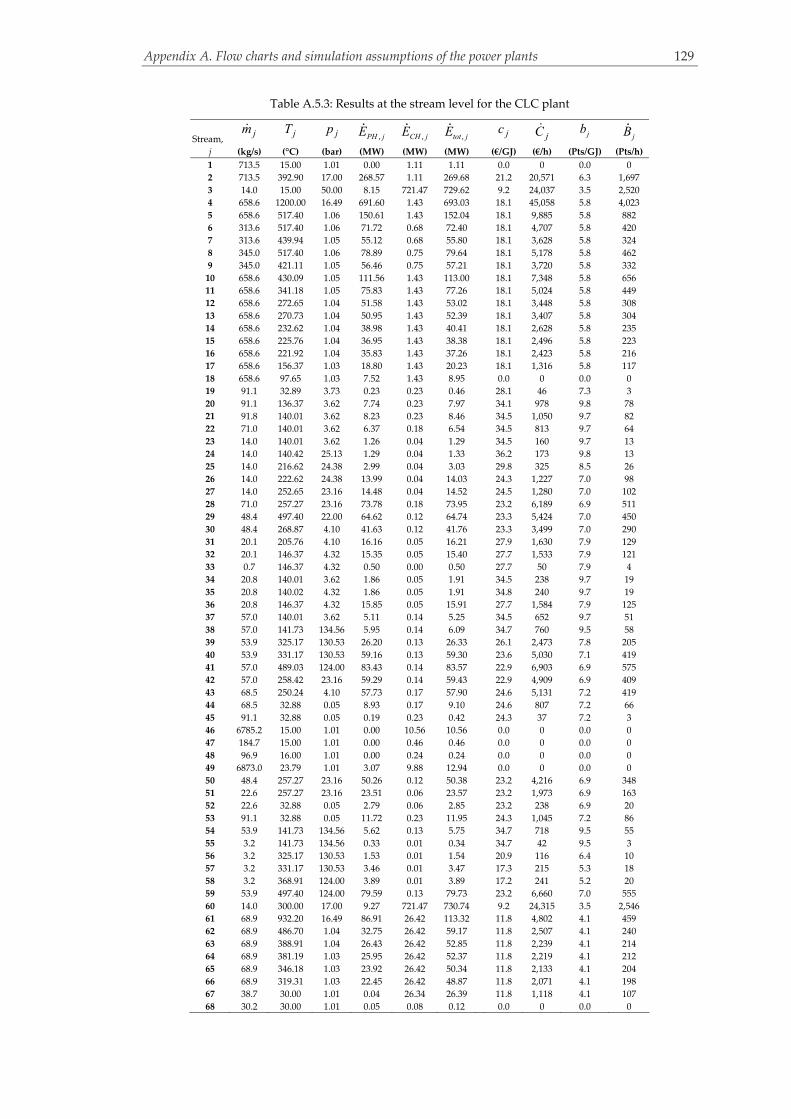
Appendix A. Flow charts and simulation assumptions of the power plants 129
Table A.5.3: Results at the stream level for the CLC plant
Stream, jm jT jp
,PH jE ,CH jE ,tot jE jc jС jb
jB
j (kg/s) (°C) (bar) (MW) (MW) (MW) (€/GJ) (€/h) (Pts/GJ) (Pts/h)
1 713.5 15.00 1.01 0.00 1.11 1.11 0.0 0 0.0 0
2 713.5 392.90 17.00 268.57 1.11 269.68 21.2 20,571 6.3 1,697
3 14.0 15.00 50.00 8.15 721.47 729.62 9.2 24,037 3.5 2,520
4 658.6 1200.00 16.49 691.60 1.43 693.03 18.1 45,058 5.8 4,023
5 658.6 517.40 1.06 150.61 1.43 152.04 18.1 9,885 5.8 882
6 313.6 517.40 1.06 71.72 0.68 72.40 18.1 4,707 5.8 420
7 313.6 439.94 1.05 55.12 0.68 55.80 18.1 3,628 5.8 324
8 345.0 517.40 1.06 78.89 0.75 79.64 18.1 5,178 5.8 462
9 345.0 421.11 1.05 56.46 0.75 57.21 18.1 3,720 5.8 332
10 658.6 430.09 1.05 111.56 1.43 113.00 18.1 7,348 5.8 656
11 658.6 341.18 1.05 75.83 1.43 77.26 18.1 5,024 5.8 449
12 658.6 272.65 1.04 51.58 1.43 53.02 18.1 3,448 5.8 308
13 658.6 270.73 1.04 50.95 1.43 52.39 18.1 3,407 5.8 304
14 658.6 232.62 1.04 38.98 1.43 40.41 18.1 2,628 5.8 235
15 658.6 225.76 1.04 36.95 1.43 38.38 18.1 2,496 5.8 223
16 658.6 221.92 1.04 35.83 1.43 37.26 18.1 2,423 5.8 216
17 658.6 156.37 1.03 18.80 1.43 20.23 18.1 1,316 5.8 117
18 658.6 97.65 1.03 7.52 1.43 8.95 0.0 0 0.0 0
19 91.1 32.89 3.73 0.23 0.23 0.46 28.1 46 7.3 3
20 91.1 136.37 3.62 7.74 0.23 7.97 34.1 978 9.8 78
21 91.8 140.01 3.62 8.23 0.23 8.46 34.5 1,050 9.7 82
22 71.0 140.01 3.62 6.37 0.18 6.54 34.5 813 9.7 64
23 14.0 140.01 3.62 1.26 0.04 1.29 34.5 160 9.7 13
24 14.0 140.42 25.13 1.29 0.04 1.33 36.2 173 9.8 13
25 14.0 216.62 24.38 2.99 0.04 3.03 29.8 325 8.5 26
26 14.0 222.62 24.38 13.99 0.04 14.03 24.3 1,227 7.0 98
27 14.0 252.65 23.16 14.48 0.04 14.52 24.5 1,280 7.0 102
28 71.0 257.27 23.16 73.78 0.18 73.95 23.2 6,189 6.9 511
29 48.4 497.40 22.00 64.62 0.12 64.74 23.3 5,424 7.0 450
30 48.4 268.87 4.10 41.63 0.12 41.76 23.3 3,499 7.0 290
31 20.1 205.76 4.10 16.16 0.05 16.21 27.9 1,630 7.9 129
32 20.1 146.37 4.32 15.35 0.05 15.40 27.7 1,533 7.9 121
33 0.7 146.37 4.32 0.50 0.00 0.50 27.7 50 7.9 4
34 20.8 140.01 3.62 1.86 0.05 1.91 34.5 238 9.7 19
35 20.8 140.02 4.32 1.86 0.05 1.91 34.8 240 9.7 19
36 20.8 146.37 4.32 15.85 0.05 15.91 27.7 1,584 7.9 125
37 57.0 140.01 3.62 5.11 0.14 5.25 34.5 652 9.7 51
38 57.0 141.73 134.56 5.95 0.14 6.09 34.7 760 9.5 58
39 53.9 325.17 130.53 26.20 0.13 26.33 26.1 2,473 7.8 205
40 53.9 331.17 130.53 59.16 0.13 59.30 23.6 5,030 7.1 419
41 57.0 489.03 124.00 83.43 0.14 83.57 22.9 6,903 6.9 575
42 57.0 258.42 23.16 59.29 0.14 59.43 22.9 4,909 6.9 409
43 68.5 250.24 4.10 57.73 0.17 57.90 24.6 5,131 7.2 419
44 68.5 32.88 0.05 8.93 0.17 9.10 24.6 807 7.2 66
45 91.1 32.88 0.05 0.19 0.23 0.42 24.3 37 7.2 3
46 6785.2 15.00 1.01 0.00 10.56 10.56 0.0 0 0.0 0
47 184.7 15.00 1.01 0.00 0.46 0.46 0.0 0 0.0 0
48 96.9 16.00 1.01 0.00 0.24 0.24 0.0 0 0.0 0
49 6873.0 23.79 1.01 3.07 9.88 12.94 0.0 0 0.0 0
50 48.4 257.27 23.16 50.26 0.12 50.38 23.2 4,216 6.9 348
51 22.6 257.27 23.16 23.51 0.06 23.57 23.2 1,973 6.9 163
52 22.6 32.88 0.05 2.79 0.06 2.85 23.2 238 6.9 20
53 91.1 32.88 0.05 11.72 0.23 11.95 24.3 1,045 7.2 86
54 53.9 141.73 134.56 5.62 0.13 5.75 34.7 718 9.5 55
55 3.2 141.73 134.56 0.33 0.01 0.34 34.7 42 9.5 3
56 3.2 325.17 130.53 1.53 0.01 1.54 20.9 116 6.4 10
57 3.2 331.17 130.53 3.46 0.01 3.47 17.3 215 5.3 18
58 3.2 368.91 124.00 3.89 0.01 3.89 17.2 241 5.2 20
59 53.9 497.40 124.00 79.59 0.13 79.73 23.2 6,660 7.0 555
60 14.0 300.00 17.00 9.27 721.47 730.74 9.2 24,315 3.5 2,546
61 68.9 932.20 16.49 86.91 26.42 113.32 11.8 4,802 4.1 459
62 68.9 486.70 1.04 32.75 26.42 59.17 11.8 2,507 4.1 240
63 68.9 388.91 1.04 26.43 26.42 52.85 11.8 2,239 4.1 214
64 68.9 381.19 1.03 25.95 26.42 52.37 11.8 2,219 4.1 212
65 68.9 346.18 1.03 23.92 26.42 50.34 11.8 2,133 4.1 204
66 68.9 319.31 1.03 22.45 26.42 48.87 11.8 2,071 4.1 198
67 38.7 30.00 1.01 0.04 26.34 26.39 11.8 1,118 4.1 107
68 30.2 30.00 1.01 0.05 0.08 0.12 0.0 0 0.0 0

Appendix A. Flow charts and simulation assumptions of the power plants 130
69 38.7 136.22 3.22 3.28 26.34 29.63 28.6 3,053 8.0 238
70 38.4 40.00 3.21 2.51 26.34 28.85 28.6 2,973 8.0 232
71 0.3 40.00 3.21 0.00 0.00 0.00 0.0 0 0.0 0
72 38.4 149.82 10.22 5.83 26.34 32.17 33.5 3,886 8.5 275
73 38.1 40.00 10.21 4.91 26.35 31.26 33.5 3,775 8.5 267
74 0.3 40.00 10.21 0.00 0.00 0.00 0.0 0 0.0 0
75 38.1 149.84 32.46 8.18 26.35 34.53 37.8 4,703 9.0 311
76 38.0 40.00 32.45 7.32 26.36 33.68 37.8 4,587 9.0 304
77 0.1 40.00 32.45 0.00 0.00 0.00 0.0 0 0.0 0
78 38.0 150.79 103.09 10.58 26.36 36.94 41.5 5,525 9.4 348
79 38.0 30.00 103.09 9.70 26.37 36.08 0.0 0 0.0 0
80 0.0 30.00 103.09 0.00 0.00 0.00 0.0 0 0.0 0
81 14.0 15.00 17.02 5.90 721.47 727.37 ‐ ‐ ‐ ‐
82 6859.0 16.00 1.37 0.30 17.13 17.43 ‐ ‐ ‐ ‐
83 6859.0 22.88 1.33 3.25 17.13 20.39 ‐ ‐ ‐ ‐
84 9693.2 23.79 1.33 5.64 24.21 29.85 ‐ ‐ ‐ ‐
85 2834.2 26.00 1.33 2.52 7.08 9.60 ‐ ‐ ‐ ‐
86 2731.6 26.00 1.33 2.43 6.82 9.25 ‐ ‐ ‐ ‐
87 2634.5 26.00 1.33 2.34 6.58 8.92 ‐ ‐ ‐ ‐
88 2525.9 26.00 1.33 2.24 6.31 8.55 ‐ ‐ ‐ ‐
89 2424.5 26.00 1.33 2.15 6.06 8.21 ‐ ‐ ‐ ‐
90 2424.5 16.00 1.37 0.11 6.06 6.16 ‐ ‐ ‐ ‐
91 9283.5 16.00 1.37 0.40 23.19 23.59 ‐ ‐ ‐ ‐
92 9384.9 16.00 1.37 0.41 23.44 23.85 ‐ ‐ ‐ ‐
93 9493.5 16.00 1.37 0.41 23.71 24.13 ‐ ‐ ‐ ‐
94 9590.6 16.00 1.37 0.42 23.96 24.37 ‐ ‐ ‐ ‐
95 9693.2 16.00 1.01 0.07 24.21 24.28 ‐ ‐ ‐ ‐
96 9693.2 16.00 1.37 0.42 24.21 24.63 ‐ ‐ ‐ ‐
97 101.4 16.00 1.37 0.00 0.25 0.26 ‐ ‐ ‐ ‐
98 101.4 26.00 1.33 0.09 0.25 0.34 ‐ ‐ ‐ ‐
99 108.6 16.00 1.37 0.00 0.27 0.28 ‐ ‐ ‐ ‐
100 108.6 26.00 1.33 0.10 0.27 0.37 ‐ ‐ ‐ ‐
101 97.1 16.00 1.37 0.00 0.24 0.25 ‐ ‐ ‐ ‐
102 97.1 26.00 1.33 0.09 0.24 0.33 ‐ ‐ ‐ ‐
103 102.6 16.00 1.37 0.00 0.26 0.26 ‐ ‐ ‐ ‐
104 102.6 26.00 1.33 0.09 0.26 0.35 ‐ ‐ ‐ ‐
105 22.6 45.81 0.10 4.56 0.06 4.61 ‐ ‐ ‐ ‐
106 C1 281.78 19.3 19,606 6.0 1,697
107 ST1 22.41 26.6 2,142 7.6 171
108 ST2 21.57 27.3 2,121 7.6 163
109 ST3 42.17 32.5 4,933 8.8 370
110 COND P 0.04 20.9 3 6.3 0
111 LPP 0.00 20.9 0 6.3 0
112 HPP 0.98 20.9 74 6.3 6
113 IPP 0.05 20.9 4 6.3 0
114 GT1 239.56 19.3 16,669 6.0 1,443
115 GT2 51.35 13.6 2,511 4.3 219
116 C2 3.85 36.5 507 10.0 38
117 C2 3.96 36.5 521 10.0 39
118 C3 3.91 36.5 514 10.0 39
119 C4 3.93 36.5 517 10.0 39
120 ST4 15.66 36.5 2,061 10.0 156
tot 375.99 20.9 28,295 6.3 2,360

Appendix A. Flow charts and simulation assumptions of the power plants 131
Table A.5.4: Splitting the exergy destruction in the CLC plant (MW)
Component, k ,realD kE ,
END kE ,
EXD kE ,
AVD kE ,
UND kE
,,UN END kE
,,UN EXD kE
,,AV END kE
,,AV EXD kE
C1 13.21 7.79 5.42 5.94 7.27 4.26 3.01 3.53 2.41
CLC 194.06 166.54 27.52 64.72 129.34 109.49 19.85 57.05 7.67
GT1 16.01 13.00 3.01 7.69 8.31 6.33 1.98 6.67 1.03
GT2 2.02 1.49 0.54 1.21 0.81 0.60 0.22 0.89 0.32
NGPH 5.20 2.98 2.22 0.04 5.17 2.84 2.33 0.14 ‐0.10
HPSH 1.99 0.66 1.33 0.68 1.31 0.57 0.74 0.09 0.59
HPEV 2.77 1.26 1.51 0.79 1.98 1.03 0.95 0.23 0.56
HPEC 3.67 1.86 1.80 0.94 2.72 1.55 1.17 0.31 0.63
RH 2.24 1.35 0.89 0.69 1.55 1.00 0.55 0.34 0.34
IPSH 0.14 0.15 ‐0.01 0.11 0.03 0.03 0.00 0.11 0.00
IPEV 0.97 0.85 0.12 0.40 0.57 0.46 0.11 0.39 0.01
IPEC 0.33 0.21 0.12 0.10 0.23 0.23 0.01 ‐0.02 0.12
LPSH 0.32 0.17 0.14 0.21 0.11 0.05 0.06 0.13 0.08
LPEV 3.03 1.52 1.52 0.83 2.20 1.24 0.97 0.28 0.55
LPEC 3.76 2.26 1.50 1.65 2.11 1.13 0.98 1.14 0.52
SH II 0.05 0.02 0.03 0.04 0.02 0.01 0.01 0.01 0.02
EV II 0.10 0.04 0.05 0.05 0.05 0.03 0.02 0.02 0.03
EC II 0.27 0.16 0.11 0.13 0.14 0.10 0.04 0.06 0.07
HPST 1.39 0.81 0.57 0.73 0.66 0.37 0.29 0.44 0.28
IPST 1.08 0.81 0.27 0.45 0.62 0.45 0.17 0.36 0.10
LPST 5.99 4.33 1.66 2.48 3.51 2.53 0.97 1.79 0.69
ST4 5.06 2.82 2.25 4.32 0.74 0.41 0.33 2.40 1.92
COND P 0.00 0.00 0.00 0.00 0.00 0.00 0.00 0.00 0.00
HPP 0.09 0.05 0.04 0.06 0.03 0.02 0.01 0.03 0.03
IPP 0.01 0.01 0.00 0.01 0.00 0.00 0.00 0.01 0.00
LPP 0.00 0.00 0.00 0.00 0.00 0.00 0.00 0.00 0.00
C1 0.61 0.43 0.18 0.46 0.15 0.10 0.05 0.33 0.13
C2 0.64 0.47 0.18 0.50 0.15 0.11 0.04 0.36 0.13
C3 0.64 0.47 0.17 0.50 0.15 0.10 0.04 0.37 0.13
C4 0.67 0.49 0.18 0.52 0.15 0.10 0.04 0.38 0.14
FG COND 20.31 14.84 5.47 ‐ ‐ ‐ ‐ ‐ ‐
COOL1 0.69 0.31 0.38 ‐ ‐ ‐ ‐ ‐ ‐
COOL2 0.82 0.40 0.42 ‐ ‐ ‐ ‐ ‐ ‐
COOL3 0.77 0.37 0.39 ‐ ‐ ‐ ‐ ‐ ‐
COOL4 0.78 0.36 0.41 ‐ ‐ ‐ ‐ ‐ ‐
COND 8.57 5.62 2.95 ‐ ‐ ‐ ‐ ‐ ‐
CT 3.06 2.23 0.83 ‐ ‐ ‐ ‐ ‐ ‐
MOT1 0.01 0.00 0.00 0.00 0.00 0.00 0.00 0.00 0.00
MOT2 0.00 0.00 0.00 0.00 0.00 0.00 0.00 0.00 0.00
MOT3 0.05 0.02 0.03 0.03 0.02 0.01 0.01 0.02 0.02
MOT4 0.01 0.00 0.00 0.01 0.00 0.00 0.00 0.00 0.00
GEN1 1.31 0.99 0.32 0.88 0.43 0.33 0.10 0.67 0.21
GEN2 3.65 3.99 ‐0.34 2.44 1.20 1.32 ‐0.11 2.67 ‐0.23
GEN3 0.78 0.62 0.16 0.52 0.26 0.21 0.05 0.42 0.11
Total 307.13 242.77 64.36
Total (%) 79.04 20.96

Appendix A. Flow charts and simulation assumptions of the power plants 132
Table A.5.5: Splitting the investment cost rate in the CLC plant (€/h)
AVkZ
UNkZ
Component, k realkZ
UNkZ
AVkZ
ENkZ
EXkZ
,AV ENkZ
,AV EXkZ
,UN ENkZ
,UN EXkZ
C1 964.4 819.7 144.7 564.7 399.7 84.7 59.9 480.0 339.7
CLC 4974.5 3979.6 994.9 4211.1 763.3 842.2 152.7 3368.9 610.7
GT1 1102.2 992.0 110.2 839.6 262.6 84.0 26.3 755.6 236.4
GT2 215.8 194.2 21.6 158.5 57.3 15.8 5.7 142.6 51.6
NGPH 10.2 2.7 7.6 5.6 4.6 4.2 3.4 1.5 1.2
HPSH 105.2 40.6 64.6 46.0 59.2 28.2 36.4 17.8 22.9
HPEV 139.7 71.4 68.3 72.7 67.0 35.5 32.7 37.2 34.3
HPEC 56.3 30.3 26.0 32.1 24.2 14.9 11.2 17.3 13.0
RH 53.6 25.0 28.6 34.7 18.9 18.5 10.1 16.2 8.8
IPSH 7.8 2.5 5.3 8.9 ‐1.1 6.0 ‐0.7 2.8 ‐0.3
IPEV 90.7 38.5 52.2 73.2 17.5 42.1 10.0 31.1 7.4
IPEC 8.6 4.1 4.5 8.3 0.2 4.3 0.1 4.0 0.1
LPSH 13.5 5.0 8.5 6.0 7.5 3.8 4.7 2.2 2.8
LPEV 135.2 64.8 70.4 75.8 59.3 39.5 30.9 36.3 28.4
LPEC 72.5 35.0 37.5 38.8 33.8 20.1 17.5 18.7 16.3
SH II 3.8 1.2 2.6 1.9 1.8 1.3 1.3 0.6 0.6
EV II 10.5 5.4 5.2 5.4 5.2 2.6 2.6 2.7 2.6
EC II 2.5 1.6 0.9 1.8 0.7 0.6 0.2 1.2 0.4
HPST 102.8 92.5 10.3 57.8 45.0 5.8 4.5 52.0 40.5
IPST 148.5 133.6 14.8 107.5 40.9 10.8 4.1 96.8 36.8
LPST 386.9 348.2 38.7 279.8 107.1 28.0 10.7 251.8 96.4
ST4 156.5 140.9 15.7 86.5 70.1 8.6 7.0 77.8 63.1
COND P 5.6 4.8 0.8 4.1 1.5 0.6 0.2 3.5 1.3
HPP 28.9 24.6 4.3 15.3 13.6 2.3 2.0 13.0 11.6
IPP 8.4 7.2 1.3 7.1 1.3 1.1 0.2 6.1 1.1
LPP 2.0 1.7 0.3 0.0 2.0 0.0 0.3 0.0 1.7
C1 313.8 266.7 47.1 216.8 97.0 32.5 14.6 184.3 82.5
C2 322.8 274.3 48.4 230.7 92.0 34.6 13.8 196.1 78.2
C3 318.4 270.7 47.8 228.8 89.6 34.3 13.4 194.5 76.2
C4 320.0 272.0 48.0 230.3 89.7 34.5 13.5 195.7 76.3
FG COND 69.1
COOL1 8.6
COOL2 8.5
COOL3 7.7
COOL4 10.0
COND 10.2

Appendix A. Flow charts and simulation assumptions of the power plants 133
Table A.5.6: Splitting the cost rate of exergy destruction in the CLC plant (€/h)
,realD kC ,
UND kC ,
AVD kC
,END kC ,
EXD kC
,AVD kC
,UND kC
Component, k ,
,AV END kC
,,AV EXD kC
,
,UN END kC
,,UN EXD kC
C1 919.2 506.0 413.2 542.0 377.2 245.7 167.5 296.3 209.7
CLC 6390.8 4259.4 2131.4 5484.5 906.3 1878.7 252.7 3605.8 653.6
GT1 1277.8 540.4 737.4 845.2 432.6 433.5 303.9 411.7 128.8
GT2 118.9 34.5 84.4 63.0 55.9 37.6 46.8 25.3 9.2
NGPH 220.5 5.7 214.8 126.3 94.2 5.9 208.9 120.4 ‐114.7
HPSH 129.7 85.3 44.4 43.0 86.7 5.8 38.7 37.3 48.0
HPEV 180.1 129.0 51.1 81.9 98.2 14.7 36.3 67.2 61.9
HPEC 238.5 177.0 61.4 121.2 117.2 20.3 41.1 101.0 76.1
RH 145.8 38.9 106.9 87.7 58.1 22.4 84.5 65.3 ‐26.4
IPSH 9.0 2.0 7.0 9.5 ‐0.5 7.3 ‐0.2 2.2 ‐0.3
IPEV 63.3 37.1 26.2 55.2 8.1 25.3 0.9 29.9 7.1
IPEC 21.6 15.1 6.5 13.7 7.9 ‐1.0 7.5 14.7 0.4
LPSH 20.5 7.1 13.4 11.3 9.2 8.2 5.2 3.1 3.9
LPEV 197.3 143.3 54.0 98.7 98.6 18.3 35.7 80.4 62.9
LPEC 244.7 137.2 107.5 147.3 97.4 74.0 33.6 73.3 63.9
SH II 2.3 0.7 1.6 0.9 1.4 0.6 1.0 0.3 0.3
EV II 4.1 2.1 2.0 1.9 2.2 0.8 1.2 1.1 1.0
EC II 11.3 5.8 5.5 6.7 4.6 2.5 3.0 4.3 1.6
HPST 142.8 54.6 88.2 67.2 75.6 36.5 51.7 30.7 23.9
IPST 117.9 52.3 65.6 67.7 50.2 29.8 35.8 37.9 14.4
LPST 587.3 310.7 276.7 383.6 203.8 158.9 117.8 224.6 86.0
ST4 423.8 62.3 361.5 235.6 188.2 201.2 160.3 34.4 27.9
COND P 0.7 0.1 0.6 0.2 0.5 0.1 0.5 0.1 0.0
HPP 10.9 2.3 8.6 3.6 7.3 2.4 6.2 1.2 1.1
IPP 1.2 0.1 1.1 0.6 0.6 0.5 0.6 0.1 0.0
LPP 0.1 0.0 0.1 0.0 0.1 0.0 0.1 0.0 0.0
C1 80.4 19.6 60.8 56.9 23.5 43.4 17.4 13.6 6.1
C2 84.7 19.5 65.2 61.6 23.1 47.6 17.6 13.9 5.6
C3 84.6 19.2 65.4 61.8 22.8 48.0 17.4 13.8 5.4
C4 87.8 19.2 68.7 64.3 23.6 50.5 18.2 13.8 5.4
FG COND 952.8 632.3 320.5
COOL1 79.8 32.1 47.6
COOL2 110.3 48.0 62.3
COOL3 115.5 50.6 64.9
COOL4 129.3 54.3 75.0
COND 1007.8 491.2 516.7

Appendix A. Flow charts and simulation assumptions of the power plants 134
Table A.5.7: Splitting the environmental impact of exergy destruction in the CLC plant (Pts/h)
, realD kB ,
UND kB ,
AVD kB
, END kB ,
EXD kB
, AVD kB
,UND kB
Component, k ,
, AV END kB
,,
AV EXD kB
,
,UN END kB
,,UN EXD kB
C1 79.6 43.8 35.8 46.9 32.7 21.3 14.5 25.7 18.2
CLC 671.8 447.7 224.0 576.5 95.3 197.5 26.6 379.0 68.7
GT1 114.1 48.2 65.8 75.5 38.6 38.7 27.1 36.8 11.5
GT2 11.4 3.3 8.1 6.0 5.3 3.6 4.5 2.4 0.9
NGPH 21.1 0.5 20.5 12.1 9.0 0.6 20.0 11.5 ‐11.0
HPSH 11.6 7.6 4.0 3.8 7.7 0.5 3.5 3.3 4.3
HPEV 16.1 11.5 4.6 7.3 8.8 1.3 3.2 6.0 5.5
HPEC 21.3 15.8 5.5 10.8 10.5 1.8 3.7 9.0 6.8
RH 13.0 3.5 9.5 7.8 5.2 2.0 7.5 5.8 ‐2.4
IPSH 0.8 0.2 0.6 0.8 0.0 0.6 0.0 0.2 0.0
IPEV 5.6 3.3 2.3 4.9 0.7 2.3 0.1 2.7 0.6
IPEC 1.9 1.3 0.6 1.2 0.7 ‐0.1 0.7 1.3 0.0
LPSH 1.8 0.6 1.2 1.0 0.8 0.7 0.5 0.3 0.4
LPEV 17.6 12.8 4.8 8.8 8.8 1.6 3.2 7.2 5.6
LPEC 21.8 12.2 9.6 13.1 8.7 6.6 3.0 6.5 5.7
SH II 0.2 0.1 0.2 0.1 0.1 0.1 0.1 0.0 0.0
EV II 0.4 0.2 0.2 0.2 0.2 0.1 0.1 0.1 0.1
EC II 1.1 0.6 0.5 0.6 0.4 0.2 0.3 0.4 0.1
HPST 11.9 4.6 7.3 5.6 6.3 3.0 4.3 2.6 2.0
IPST 9.8 4.3 5.4 5.6 4.2 2.5 3.0 3.1 1.2
LPST 48.0 25.4 22.6 31.3 16.6 13.0 9.6 18.3 7.0
ST4 35.0 5.1 29.8 19.4 15.5 16.6 13.2 2.8 2.3
COND P 0.1 0.0 0.0 0.0 0.0 0.0 0.0 0.0 0.0
HPP 0.9 0.2 0.7 0.3 0.6 0.2 0.5 0.1 0.1
IPP 0.1 0.0 0.1 0.0 0.0 0.0 0.0 0.0 0.0
LPP 0.0 0.0 0.0 0.0 0.0 0.0 0.0 0.0 0.0
C1 6.1 1.5 4.6 4.3 1.8 3.3 1.3 1.0 0.5
C2 6.4 1.5 4.9 4.7 1.8 3.6 1.3 1.1 0.4
C3 6.4 1.5 5.0 4.7 1.7 3.6 1.3 1.0 0.4
C4 6.7 1.5 5.2 4.9 1.8 3.8 1.4 1.0 0.4
FG COND 91.1 60.4 30.6
COOL1 6.2 2.5 3.7
COOL2 7.8 3.4 4.4
COOL3 7.6 3.3 4.3
COOL4 8.1 3.4 4.7
COND 82.5 40.2 42.3

Appendix A. Flow charts and simulation assumptions of the power plants 135
GG
M
M
M
M
M
7
63
12
5
8
4
9
10
11 12
13
1415
1617
19
20
21
22
2337
34
35
25
24
32
36
31
43
29
42
41
27
28
40
26
33
38
39
40
45
66
Ch
imn
ey
67
18
59
60 61
6263
64
81
65
82
79
80
78
57
58
56
54
55
51
52
5350
49
48
47
7172
73
7574
68
69
77
44
46
C2
CO
OL1
C3
CO
OL2
C4
CO
OL3
C5
CO
OL4
CT
P
CT
LPEC
LPEV
LPSH
IPECIP
PH
PP
LPP
De-
aera
tor
CO
ND
P
CO
ND
LPST
IPST
HPS
T
GT1
C1
GEN
1
RH
HPS
H
HPE
V
HP
EC
IPSH
ST4
IPEV
GEN
2ST
5
COO
L CA
UC
6
CC
30
70
9091
9293
9483
989795
99
100
89 88
8786
85
96
101
103
102
104
106
105
107
76
M2
M3
M1
M4
M
EA-0
.2η:
50.
5%, ε
: 48.
4%W
net:
353.
8 M
W
M
EA-0
η: 4
7.8%
, ε: 4
5.8%
Wne
t: 33
4.6
MW
A.6: The MEA plant
Figure A.6.1: Structure of the MEA plant

Appendix A. Flow charts and simulation assumptions of the power plants 136
Table A.6.1: Results of the year‐by‐year economic analysis for MEA‐0.2
Ref. Plant
Debt Book Adjustment Common Equity Book Adjustment TCR
Year Calendar year beg. of year depreciation beg. of year depreciation
1 2013 213,525,868 10,676,293 703,303 213,525,868 8,078,458 1,677,021 21,135,075
2 2014 202,146,272 10,676,293 703,303 203,770,389 8,078,458 1,677,021 21,135,075
3 2015 190,766,675 10,676,293 703,303 194,014,911 8,078,458 1,677,021 21,135,075
4 2016 179,387,078 10,676,293 703,303 184,259,432 8,078,458 1,677,021 21,135,075
5 2017 168,007,482 10,676,293 703,303 174,503,953 8,078,458 1,677,021 21,135,075
6 2018 156,627,885 10,676,293 703,303 164,748,474 8,078,458 1,677,021 21,135,075
7 2019 145,248,289 10,676,293 703,303 154,992,995 8,078,458 1,677,021 21,135,075
8 2020 133,868,692 10,676,293 703,303 145,237,516 8,078,458 1,677,021 21,135,075
9 2021 122,489,095 10,676,293 703,303 135,482,037 8,078,458 1,677,021 21,135,075
10 2022 111,109,499 10,676,293 703,303 125,726,559 8,078,458 1,677,021 21,135,075
11 2023 99,729,902 10,676,293 703,303 115,971,080 8,078,458 1,677,021 21,135,075
12 2024 88,350,306 10,676,293 703,303 106,215,601 8,078,458 1,677,021 21,135,075
13 2025 76,970,709 10,676,293 703,303 96,460,122 8,078,458 1,677,021 21,135,075
14 2026 65,591,112 10,676,293 703,303 86,704,643 8,078,458 1,677,021 21,135,075
15 2027 54,211,516 10,676,293 703,303 76,949,164 8,078,458 1,677,021 21,135,075
16 2028 42,831,919 10,676,293 703,303 67,193,686 8,078,458 1,677,021 21,135,075
17 2029 31,452,323 10,676,293 ‐2,813,213 57,438,207 8,078,458 ‐1,839,495 14,102,044
18 2030 23,589,242 10,676,293 ‐2,813,213 51,199,244 8,078,458 ‐1,839,495 14,102,044
19 2031 15,726,161 10,676,293 ‐2,813,213 44,960,281 8,078,458 ‐1,839,495 14,102,044
20 2032 7,863,081 10,676,293 ‐2,813,213 38,721,318 8,078,458 ‐1,839,495 14,102,044
21 2033 0 0 0 32,482,355 0 0 0
Total 2,129,493,106 213,525,868 0 2,470,557,835 161,569,166 19,474,347 394,569,381
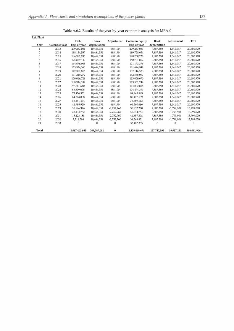
Appendix A. Flow charts and simulation assumptions of the power plants 137
Table A.6.2: Results of the year‐by‐year economic analysis for MEA‐0
Ref. Plant
Debt Book Adjustment Common Equity Book Adjustment TCR
Year Calendar year beg. of year depreciation beg. of year depreciation
1 2013 209,287,081 10,464,354 688,190 209,287,081 7,887,380 1,641,047 20,680,970
2 2014 198,134,537 10,464,354 688,190 199,758,654 7,887,380 1,641,047 20,680,970
3 2015 186,981,993 10,464,354 688,190 190,230,228 7,887,380 1,641,047 20,680,970
4 2016 175,829,449 10,464,354 688,190 180,701,802 7,887,380 1,641,047 20,680,970
5 2017 164,676,905 10,464,354 688,190 171,173,376 7,887,380 1,641,047 20,680,970
6 2018 153,524,360 10,464,354 688,190 161,644,949 7,887,380 1,641,047 20,680,970
7 2019 142,371,816 10,464,354 688,190 152,116,523 7,887,380 1,641,047 20,680,970
8 2020 131,219,272 10,464,354 688,190 142,588,097 7,887,380 1,641,047 20,680,970
9 2021 120,066,728 10,464,354 688,190 133,059,670 7,887,380 1,641,047 20,680,970
10 2022 108,914,184 10,464,354 688,190 123,531,244 7,887,380 1,641,047 20,680,970
11 2023 97,761,640 10,464,354 688,190 114,002,818 7,887,380 1,641,047 20,680,970
12 2024 86,609,096 10,464,354 688,190 104,474,391 7,887,380 1,641,047 20,680,970
13 2025 75,456,552 10,464,354 688,190 94,945,965 7,887,380 1,641,047 20,680,970
14 2026 64,304,008 10,464,354 688,190 85,417,539 7,887,380 1,641,047 20,680,970
15 2027 53,151,464 10,464,354 688,190 75,889,113 7,887,380 1,641,047 20,680,970
16 2028 41,998,920 10,464,354 688,190 66,360,686 7,887,380 1,641,047 20,680,970
17 2029 30,846,376 10,464,354 ‐2,752,760 56,832,260 7,887,380 ‐1,799,904 13,799,070
18 2030 23,134,782 10,464,354 ‐2,752,760 50,744,784 7,887,380 ‐1,799,904 13,799,070
19 2031 15,423,188 10,464,354 ‐2,752,760 44,657,308 7,887,380 ‐1,799,904 13,799,070
20 2032 7,711,594 10,464,354 ‐2,752,760 38,569,831 7,887,380 ‐1,799,904 13,799,070
21 2033 0 0 0 32,482,355 0 0 0
Total 2,087,403,945 209,287,081 0 2,428,468,674 157,747,595 19,057,131 386,091,806

Appendix A. Flow charts and simulation assumptions of the power plants 138
Table A.6.3: Results at the component level for MEA‐0.2
,F kE ,P kE ,D kE k ,D ky ,F kc ,P kc ,D kC kZ ,D k kC Z kf kr ,F kb ,P kb ,D kB kY ,D k kB Y
,b kf ,b kr
Component, k (MW) (MW) (MW) (%) (%) (€/GJ) (€/GJ) (€/h) (€/h) (€/h) (%) (%) (Pts/GJ) (Pts/GJ) (Pts/h) (Pts/h) (Pts/h) (%) (%)
C1 242.68 231.30 11.38 95.3 1.56 16.9 19.4 691 1,396 2,086 66.9 14.9 6.1 6.4 249.98 0.24 250.22 0.09 4.9CC 729.62 508.76 220.87 69.7 30.23 9.2 13.7 7,276 997 8,273 12.0 49.4 3.5 5.6 2746.20 0.38 2746.59 0.01 63.5GT 551.15 530.67 20.47 96.3 2.80 15.4 16.9 1,137 1,595 2,732 58.4 9.3 5.9 6.1 433.06 1.13 434.18 0.26 3.9HPSH 35.06 31.72 3.34 90.5 0.46 15.4 18.9 185 155 341 45.6 22.6 5.9 6.7 70.64 1.24 71.89 1.73 13.5HPEV 43.64 39.91 3.73 91.4 0.51 15.4 18.6 207 181 389 46.7 20.4 5.9 6.6 78.95 0.13 79.07 0.16 11.9HPEC 28.92 24.91 4.01 86.1 0.55 15.4 19.6 223 88 310 28.2 27.3 5.9 7.1 84.77 0.09 84.86 0.11 20.4RH 26.46 23.89 2.57 90.3 0.35 15.4 18.9 143 109 252 43.3 22.2 5.9 6.7 54.34 0.79 55.13 1.42 13.8IPSH 0.18 0.12 0.06 69.0 0.01 15.4 33.3 3 4 7 56.0 115.7 5.9 9.2 1.17 0.00 1.17 0.17 57.1IPEV 6.10 5.67 0.43 92.9 0.06 15.4 20.1 24 64 88 72.8 30.3 5.9 6.4 9.13 0.04 9.17 0.41 9.7IPEC 1.06 0.87 0.19 82.5 0.03 15.4 21.3 10 5 15 33.0 38.2 5.9 7.5 3.93 0.00 3.94 0.08 27.0LPSH 1.43 1.05 0.38 73.3 0.05 15.4 27.8 21 19 40 47.4 80.4 5.9 8.6 8.10 0.01 8.12 0.16 46.4LPEV 19.02 15.47 3.54 81.4 0.49 15.4 23.1 197 171 368 46.4 49.8 5.9 7.6 74.98 0.12 75.10 0.16 29.1LPEC 11.57 7.81 3.76 67.5 0.51 15.4 28.5 209 94 303 31.0 84.5 5.9 9.5 79.59 0.10 79.68 0.12 61.2HPST 31.29 29.18 2.11 93.2 0.29 19.7 22.6 150 122 272 44.9 14.9 6.9 7.5 52.44 0.28 52.72 0.53 8.9IPST 2.62 2.46 0.15 94.2 0.02 19.6 23.5 11 21 31 65.7 19.5 6.8 7.4 3.76 0.10 3.86 2.53 7.8LPST 40.94 35.38 5.56 86.4 0.76 21.4 27.8 428 296 723 40.9 30.0 7.2 8.6 144.91 0.32 145.23 0.22 19.2ST4 19.39 18.54 0.85 95.6 0.12 19.6 22.5 60 114 174 65.4 14.4 6.8 7.2 21.04 0.20 21.25 0.95 5.7ST5 15.39 14.71 0.68 95.6 0.09 19.6 22.4 48 86 134 64.2 14.0 6.8 7.2 16.70 0.18 16.87 1.05 5.7COND P 0.04 0.04 0.01 78.8 0.00 18.5 80.0 1 7 8 91.7 333.3 6.5 8.7 0.22 0.00 0.22 0.13 33.6HPP 1.12 0.96 0.16 85.4 0.02 18.5 34.2 11 40 51 78.8 85.2 6.5 7.9 3.83 0.00 3.83 0.01 21.4IPP 0.03 0.02 0.01 61.0 0.00 18.5 140.4 1 8 8 90.3 660.4 0.5 10.7 0.02 0.00 0.02 0.11 1886.0LPP 0.00 0.00 0.00 71.8 0.00 18.5 421.7 0 2 3 98.1 2183.8 78.1 19.4 0.21 0.00 0.21 0.05 ‐75.1De‐aerator 0.46 0.44 0.02 95.6 0.00 23.9 42.1 2 27 29 94.0 76.5 7.8 8.2 0.56 0.04 0.60 5.87 5.8C2 18.53 16.93 1.59 91.4 0.22 22.5 43.6 129 1,159 1,288 90.0 94.0 7.2 8.0 41.57 3.78 45.35 8.33 10.3C3 4.33 3.78 0.55 87.3 0.08 22.4 132.9 44 439 483 90.8 493.8 7.2 25.8 14.36 0.70 15.05 4.62 256.9C4 3.45 2.86 0.59 82.9 0.08 22.4 100.1 48 350 398 88.0 347.2 7.2 16.3 15.40 0.28 15.68 1.81 125.2C5 3.44 2.82 0.61 82.1 0.08 22.4 77.0 49 348 398 87.6 244.3 7.2 11.5 15.99 0.14 16.13 0.86 58.3C6 3.49 2.83 0.66 81.1 0.09 22.4 77.4 53 354 406 87.0 245.7 7.2 11.4 17.13 0.20 17.34 1.18 57.5M1 1.40 1.26 0.14 89.7 0.02 19.6 21.9 10 0 10 0.0 11.5 6.8 7.6 3.56 0.00 3.56 0.00 11.5M2 0.63 0.58 0.04 92.9 0.01 19.7 21.2 3 0 3 0.0 7.6 6.9 7.4 1.10 0.00 1.10 0.00 7.6M3 0.18 0.18 0.00 99.9 0.00 15.4 15.4 0 0 0 0.0 0.1 5.9 5.9 0.00 0.00 0.00 0.00 0.1M4 3.11 2.96 0.15 95.0 0.02 21.4 22.5 12 0 12 0.0 5.2 7.2 7.6 4.02 0.00 4.02 0.00 5.2CAU 59.28 ‐ 40.59 ‐ 5.56 23.7 ‐ 3,463 1,023 4,486 22.8 ‐ 6.9 ‐ 1006.53 1.75 1008.28 0.17 ‐COOL CAU 9.50 ‐ 8.54 ‐ 1.17 29.7 ‐ 914 59 974 6.1 ‐ 6.9 ‐ 213.65 0.06 213.71 0.03 ‐COOL1 2.30 ‐ 2.15 ‐ 0.29 55.7 ‐ 432 10 441 2.2 ‐ 11.7 ‐ 90.74 0.01 90.74 0.01 ‐COOL2 0.80 ‐ 0.72 ‐ 0.10 64.0 ‐ 166 8 174 4.6 ‐ 12.6 ‐ 32.59 0.01 32.59 0.02 ‐COOL3 0.75 ‐ 0.68 ‐ 0.09 66.0 ‐ 162 7 170 4.3 ‐ 12.4 ‐ 30.43 0.01 30.44 0.02 ‐COOL4 0.78 ‐ 0.70 ‐ 0.10 67.6 ‐ 171 9 180 5.0 ‐ 12.2 ‐ 30.90 0.01 30.91 0.02 ‐COND 7.03 ‐ 5.23 ‐ 0.72 21.8 ‐ 410 54 464 11.7 ‐ 7.4 ‐ 138.99 0.01 139.00 0.01 ‐CT 3.06 ‐ 1.88 ‐ 0.26 ‐ ‐ ‐ 18 ‐ ‐ ‐ ‐ ‐ ‐ 9.31 ‐ ‐ ‐Total 730.58 353.82 349.14 48.4 47.79 9.2 26.3 11,502 9,440 20,942 45.1 187.0 3.5 7.6 4341.17 21.63 4362.80 0.50 120.7Exergy loss 27.62
PFkB 1270.3
Appen
dix A. Flow charts an
d simulation
assumption
s of the power plan
ts
138

Appendix A. Flow charts and simulation assumptions of the power plants 139
Table A.6.4: Results at the component level for MEA‐0
,F kE ,P kE ,D kE k ,D ky ,F kc ,P kc ,D kC kZ ,D k kC Z
kf kr ,F kb ,P kb ,D kB kY ,D k kB Y ,b kf ,b kr
Component, k (MW) (MW) (MW) (%) (%) (€/GJ) (€/GJ) (€/h) (€/h) (€/h) (%) (%) (Pts/GJ) (Pts/GJ) (Pts/h) (Pts/h) (Pts/h) (%) (%)
C1 242.68 231.30 11.38 95.3 1.56 16.9 19.4 690 1,395 2,086 66.9 14.9 6.1 6.4 249.94 0.24 250.17 0.09 4.9CC 729.62 508.76 220.87 69.7 30.23 9.2 13.7 7,276 997 8,273 12.0 49.4 3.5 5.6 2746.20 0.38 2746.59 0.01 63.5GT 551.15 530.67 20.47 96.3 2.80 15.4 16.9 1,137 1,595 2,732 58.4 9.3 5.9 6.1 432.98 1.13 434.11 0.26 3.9HPSH 35.06 31.72 3.34 90.5 0.46 15.4 18.7 185 155 340 45.5 20.9 5.9 6.6 70.63 1.24 71.87 1.72 12.1HPEV 43.64 39.91 3.73 91.4 0.51 15.4 18.4 207 181 389 46.7 19.0 5.9 6.5 78.93 0.13 79.06 0.16 10.6HPEC 28.92 24.91 4.01 86.1 0.55 15.4 19.3 223 87 310 28.2 24.9 5.9 6.9 84.76 0.09 84.85 0.11 18.2RH 26.46 23.89 2.57 90.3 0.35 15.4 18.6 143 109 252 43.3 20.6 5.9 6.6 54.33 0.79 55.12 1.43 12.3IPSH 0.18 0.12 0.06 69.0 0.01 15.4 32.2 3 4 7 55.9 108.7 5.9 8.9 1.17 0.00 1.17 0.17 51.0IPEV 6.10 5.67 0.43 92.9 0.06 15.4 19.9 24 64 88 72.8 29.2 5.9 6.4 9.13 0.04 9.17 0.41 8.7IPEC 1.06 0.87 0.19 82.5 0.03 15.4 20.8 10 5 15 33.0 35.0 5.9 7.3 3.93 0.00 3.94 0.08 24.1LPSH 1.43 1.05 0.38 73.3 0.05 15.4 27.0 21 19 40 47.2 74.7 5.9 8.3 8.10 0.01 8.12 0.16 41.4LPEV 19.02 15.47 3.54 81.4 0.49 15.4 22.6 197 171 368 46.4 46.3 5.9 7.4 74.97 0.12 75.09 0.16 26.0LPEC 11.57 7.81 3.76 67.5 0.51 15.4 27.3 209 94 303 31.0 77.3 5.9 9.1 79.57 0.10 79.67 0.12 54.6HPST 31.29 29.18 2.11 93.2 0.29 19.4 22.1 147 127 274 46.2 14.4 6.8 7.3 51.61 0.28 51.89 0.54 8.1IPST 3.43 3.23 0.20 94.2 0.03 19.3 22.5 14 21 35 60.6 16.5 6.7 7.2 4.87 0.10 4.97 2.07 7.0LPST 17.84 15.42 2.42 86.4 0.33 22.9 29.3 200 134 334 40.1 27.9 7.5 8.8 65.52 0.19 65.71 0.29 17.4ST4 19.39 18.54 0.85 95.6 0.12 19.3 22.1 59 118 178 66.6 14.4 6.7 7.1 20.72 0.20 20.93 0.97 5.2ST5 14.57 13.93 0.64 95.6 0.09 19.3 22.1 45 89 134 66.7 14.4 6.7 7.1 15.57 0.17 15.74 1.10 5.2COND P 0.04 0.04 0.01 78.8 0.00 17.9 78.7 1 7 8 92.0 338.7 6.3 8.3 0.22 0.00 0.22 0.14 30.3HPP 1.12 0.96 0.16 85.4 0.02 17.9 33.2 11 40 51 79.2 84.9 6.3 7.6 3.75 0.00 3.75 0.01 19.3IPP 0.03 0.02 0.01 61.0 0.00 17.9 139.4 1 8 8 90.6 677.1 0.5 10.4 0.02 0.00 0.02 0.12 1880.4LPP 0.00 0.00 0.00 71.8 0.00 17.9 405.7 0 2 3 98.1 2161.2 76.4 14.0 0.20 0.00 0.20 0.05 ‐81.7De‐aerator 0.46 0.44 0.02 95.6 0.00 23.3 41.4 2 27 29 94.1 77.9 7.6 8.0 0.55 0.04 0.58 6.02 5.3C2 18.53 16.93 1.59 91.4 0.22 22.1 43.2 127 1,159 1,286 90.1 95.4 7.1 7.8 40.73 3.78 44.51 8.49 10.3C3 3.54 3.00 0.54 84.6 0.07 22.1 153.7 43 365 408 89.4 594.8 7.1 30.2 13.88 0.70 14.57 4.78 325.7C4 3.45 2.86 0.59 82.9 0.08 22.1 78.6 47 356 403 88.3 255.3 7.1 11.8 15.07 0.28 15.35 1.85 66.4C5 3.44 2.82 0.61 82.1 0.08 22.1 77.2 49 354 403 87.9 249.1 7.1 11.3 15.67 0.14 15.81 0.87 58.7C6 3.49 2.83 0.66 81.1 0.09 22.1 77.6 52 360 412 87.3 250.8 7.1 11.2 16.79 0.20 16.99 1.20 57.8M1 0.30 0.26 0.03 88.5 0.00 19.3 21.8 2 0 2 0.0 12.9 6.7 7.6 0.83 0.00 0.83 0.00 12.9M2 0.63 0.58 0.04 92.9 0.01 19.4 20.8 3 0 3 0.0 7.6 6.8 7.3 1.08 0.00 1.08 0.00 7.6M3 0.18 0.18 0.00 99.9 0.00 15.4 15.4 0 0 0 0.0 0.1 5.9 5.9 0.00 0.00 0.00 0.00 0.1M4 2.43 2.32 0.11 95.5 0.02 22.9 24.0 9 0 9 0.0 4.7 7.5 7.9 2.98 0.00 2.98 0.00 4.7CAU 86.54 ‐ 67.95 ‐ 9.30 22.1 ‐ 5,417 1,086 6,503 16.7 ‐ 6.8 ‐ 1658.02 3.50 1661.52 0.21 ‐COOL CAU 9.50 ‐ 8.54 ‐ 1.17 29.5 ‐ 908 60 968 6.2 ‐ 6.9 ‐ 211.13 0.06 211.20 0.03 ‐COOL1 0.98 ‐ 0.90 ‐ 0.12 56.7 ‐ 184 8 191 4.1 ‐ 12.0 ‐ 38.78 0.01 38.78 0.02 ‐COOL2 0.80 ‐ 0.72 ‐ 0.10 60.8 ‐ 157 8 165 4.9 ‐ 12.0 ‐ 30.92 0.01 30.93 0.02 ‐COOL3 0.75 ‐ 0.68 ‐ 0.09 63.4 ‐ 156 7 163 4.5 ‐ 11.8 ‐ 29.10 0.01 29.10 0.02 ‐COOL4 0.78 ‐ 0.70 ‐ 0.10 65.4 ‐ 165 9 174 5.2 ‐ 11.7 ‐ 29.65 0.01 29.66 0.02 ‐COND 3.02 ‐ 2.25 ‐ 0.31 23.4 ‐ 190 26 216 12.1 ‐ 7.7 ‐ 62.38 0.01 62.38 0.01 ‐CT 1.99 ‐ 1.17 ‐ 0.16 ‐ ‐ ‐ 11 ‐ ‐ ‐ ‐ ‐ ‐ 5.34 ‐ ‐ ‐
Total 730.58 334.63 368.27 45.8 50.41 9.2 27.6 12,133 9,257 21,390 43.3 201.9 67.8 73.0 4579.01 19.27 4598.28 0.42 7.6
Exergy loss 27.68 PFkB 1268.4
Appen
dix A. Flow charts an
d simulation
assumption
s of the power plan
ts
139

Appendix A. Flow charts and simulation assumptions of the power plants 140
Table A.6.5: Results at the stream level for MEA‐0.2
Stream, jm jT jp
,PH jE ,CH jE ,tot jE jc jС jb
jB
j (kg/s) (°C) (bar) (MW) (MW) (MW) (€/GJ) (€/h) (Pts/GJ) (Pts/h)
1 614.50 15.00 1.01 0.00 0.96 0.96 0.00 0 0.0 0
2 614.50 392.90 17.00 231.30 0.96 232.25 19.28 16,124 6.4 5,332
3 14.00 15.00 50.00 8.15 721.47 729.62 9.15 24,037 3.5 9,072
4 628.50 1264.03 16.49 735.74 5.27 741.01 15.43 41,158 5.9 15,675
5 628.50 580.64 1.06 184.60 5.27 189.87 15.43 10,546 5.9 4,016
6 268.50 580.64 1.06 78.86 2.25 81.11 15.43 4,505 5.9 1,716
7 268.50 447.62 1.05 52.40 2.25 54.65 15.43 3,035 5.9 1,156
8 360.00 580.64 1.06 105.73 3.02 108.75 15.43 6,040 5.9 2,300
9 360.00 449.30 1.05 70.67 3.02 73.69 15.43 4,093 5.9 1,559
10 628.50 448.58 1.04 123.07 5.27 128.34 15.43 7,128 5.9 2,715
11 628.50 341.18 1.04 79.43 5.27 84.70 15.43 4,704 5.9 1,792
12 628.50 257.91 1.04 50.51 5.27 55.78 15.43 3,098 5.9 1,180
13 628.50 257.35 1.04 50.33 5.27 55.60 15.43 3,088 5.9 1,176
14 628.50 237.62 1.04 44.23 5.27 49.50 15.43 2,749 5.9 1,047
15 628.50 234.08 1.04 43.17 5.27 48.44 15.43 2,690 5.9 1,025
16 628.50 229.24 1.04 41.73 5.27 47.00 15.43 2,611 5.9 994
17 628.50 156.37 1.03 22.72 5.27 27.99 15.43 1,554 5.9 592
18 628.50 94.79 1.03 11.14 5.27 16.41 0.00 0 0.0 0
19 94.71 32.89 3.73 0.24 0.24 0.47 26.10 44 7.5 13
20 94.71 136.37 3.62 8.05 0.24 8.28 28.33 845 9.4 279
21 95.40 140.01 3.62 8.55 0.24 8.79 28.99 917 9.3 294
22 72.43 140.01 3.62 6.49 0.18 6.67 28.99 696 9.3 223
23 7.22 140.01 3.62 0.65 0.02 0.67 28.99 69 9.3 22
24 7.22 140.49 25.13 0.67 0.02 0.68 32.12 79 9.3 23
25 7.22 216.62 24.38 1.54 0.02 1.56 26.06 146 8.3 46
26 7.22 222.62 24.38 7.21 0.02 7.23 21.39 557 6.8 178
27 7.22 237.91 23.16 7.33 0.02 7.35 21.59 571 6.9 182
28 72.43 305.14 23.16 79.35 0.18 79.53 19.87 5,689 6.9 1,975
29 72.43 560.64 22.00 103.24 0.18 103.42 19.64 7,311 6.8 2,550
30 39.00 9.85 3.90 0.02 0.10 0.12 19.64 8 6.8 3
31 22.28 214.08 4.10 18.06 0.06 18.12 24.09 1,571 7.8 511
32 22.28 146.37 4.32 17.01 0.06 17.07 23.85 1,466 7.8 479
33 0.68 146.37 4.32 0.52 0.00 0.52 23.85 45 7.8 15
34 22.96 140.01 3.62 2.06 0.06 2.12 28.99 221 9.3 71
35 22.96 140.02 4.32 2.06 0.06 2.12 29.34 224 9.3 71
36 22.96 146.37 4.32 17.53 0.06 17.59 23.85 1,511 7.8 493
37 65.21 140.01 3.62 5.84 0.16 6.01 28.99 627 9.3 201
38 65.21 141.75 134.56 6.80 0.16 6.96 29.70 745 9.1 228
39 65.21 325.17 130.53 31.72 0.16 31.88 21.84 2,506 7.5 863
40 65.21 331.17 130.53 71.63 0.16 71.79 20.02 5,175 7.0 1,807
41 65.21 560.64 124.00 103.35 0.16 103.51 19.68 7,334 6.9 2,569
42 65.21 313.21 23.16 72.06 0.16 72.22 19.68 5,117 6.9 1,793
43 55.71 275.88 4.10 48.31 0.14 48.45 21.36 3,725 7.2 1,263
44 55.71 32.88 0.05 7.37 0.14 7.51 21.36 577 7.2 196
45 94.71 32.88 0.05 0.20 0.24 0.44 21.77 34 7.4 12
46 628.50 122.27 1.30 28.08 5.27 33.35 29.73 3,569 6.9 834
47 628.50 51.00 1.30 18.58 5.27 23.85 29.73 2,552 6.9 596
48 595.25 46.74 1.03 5.98 1.47 7.45 181.88 4,877 44.4 1,191
49 33.25 139.10 1.03 0.67 10.57 11.24 29.73 1,203 6.9 281
50 33.25 267.18 3.22 4.45 10.57 15.02 55.68 3,010 11.7 632
51 33.23 40.00 3.20 2.14 10.57 12.71 55.68 2,548 11.7 535
52 0.01 40.00 3.20 0.00 0.00 0.00 0.00 0 0.0 0
53 33.23 151.78 10.22 5.01 10.57 15.58 63.84 3,580 12.5 704
54 33.01 40.00 10.21 4.20 10.58 14.78 63.84 3,396 12.5 667
55 0.22 40.00 10.21 0.00 0.00 0.00 0.00 0 0.0 0
56 33.01 152.67 32.46 7.02 10.58 17.60 65.96 4,179 12.4 784
57 32.94 40.00 32.45 6.25 10.59 16.84 65.96 3,999 12.4 750

Appendix A. Flow charts and simulation assumptions of the power plants 141
58 0.07 40.00 32.45 0.00 0.00 0.00 0.00 0 0.0 0
59 32.94 154.69 103.09 9.08 10.59 19.67 67.60 4,787 12.2 866
60 32.92 30.00 103.09 8.30 10.60 18.89 0.00 0 0.0 0
61 0.03 30.00 103.09 0.00 0.00 0.00 0.00 0 0.0 0
62 4036.07 15.00 1.01 0.00 6.28 6.28 0.00 0 0.0 0
63 109.58 15.00 1.01 0.00 0.27 0.27 0.00 0 0.0 0
64 57.66 16.00 1.01 0.00 0.14 0.14 0.00 0 0.0 0
65 4088.00 23.73 1.01 1.80 5.87 7.67 0.00 0 0.0 0
66 39.00 317.23 4.10 35.45 0.10 35.55 19.64 2,513 6.8 877
67 33.43 317.23 4.10 30.39 0.08 30.48 19.64 2,154 6.8 751
68 94.71 32.88 0.05 7.23 0.24 7.47 21.77 586 7.4 199
69 72.43 317.23 4.10 65.85 0.18 66.03 19.64 4,668 6.8 1,628
70 5.07 317.23 4.10 4.61 0.01 4.62 19.64 327 6.8 114
71 67.37 317.23 4.10 61.24 0.17 61.41 19.64 4,341 6.8 1,514
72 29.80 317.23 4.10 27.09 0.07 27.17 19.64 1,920 6.8 670
73 29.80 560.64 22.00 42.48 0.07 42.55 19.64 3,008 6.8 1,049
74 37.56 560.64 22.00 53.54 0.09 53.63 19.64 3,791 6.8 1,322
75 37.56 317.23 4.10 34.15 0.09 34.24 19.64 2,421 6.8 844
76 67.37 560.64 22.00 96.02 0.17 96.19 19.64 6,799 6.8 2,372
77 5.07 560.64 22.00 7.22 0.01 7.24 19.64 511 6.8 178
78 5765.82 16.00 1.37 0.25 14.40 14.65 ‐ ‐ ‐ ‐
79 5765.82 16.00 1.01 0.04 14.40 14.44 ‐ ‐ ‐ ‐
80 1580.32 26.00 1.33 1.40 3.95 5.35 ‐ ‐ ‐ ‐
81 5765.82 23.73 1.33 3.31 14.40 17.72 ‐ ‐ ‐ ‐
82 4185.50 22.88 1.33 1.99 10.45 12.44 ‐ ‐ ‐ ‐
83 4185.50 16.00 1.37 0.18 10.45 10.64 ‐ ‐ ‐ ‐
84 5320.01 16.00 1.37 0.23 13.29 13.52 ‐ ‐ ‐ ‐
85 5495.45 16.00 1.37 0.24 13.73 13.97 ‐ ‐ ‐ ‐
86 5589.87 16.00 1.37 0.24 13.96 14.21 ‐ ‐ ‐ ‐
87 5675.09 16.00 1.37 0.25 14.18 14.42 ‐ ‐ ‐ ‐
88 90.73 16.00 1.37 0.00 0.23 0.23 ‐ ‐ ‐ ‐
89 90.73 26.00 1.33 0.08 0.23 0.31 ‐ ‐ ‐ ‐
90 1489.59 26.00 1.33 1.32 3.72 5.04 ‐ ‐ ‐ ‐
91 1404.37 26.00 1.33 1.25 3.51 4.76 ‐ ‐ ‐ ‐
92 1309.95 26.00 1.33 1.16 3.27 4.44 ‐ ‐ ‐ ‐
93 1134.51 26.00 1.33 1.01 2.83 3.84 ‐ ‐ ‐ ‐
94 1134.51 16.00 1.37 0.05 2.83 2.88 ‐ ‐ ‐ ‐
95 175.44 26.00 1.33 0.16 0.44 0.59 ‐ ‐ ‐ ‐
96 175.44 16.00 1.37 0.01 0.44 0.45 ‐ ‐ ‐ ‐
97 94.42 26.00 1.33 0.08 0.24 0.32 ‐ ‐ ‐ ‐
98 94.42 16.00 1.37 0.00 0.24 0.24 ‐ ‐ ‐ ‐
99 85.22 26.00 1.33 0.08 0.21 0.29 ‐ ‐ ‐ ‐
100 85.22 16.00 1.37 0.00 0.21 0.22 ‐ ‐ ‐ ‐
101 39.00 9.94 0.05 0.00 0.10 0.10 ‐ ‐ ‐ ‐
102 14.00 15.00 17.00 5.90 721.47 727.37 ‐ ‐ ‐ ‐
103 498.50 392.90 17.00 187.64 0.78 188.41 ‐ ‐ ‐ ‐
104 512.50 1435.04 16.49 704.31 5.80 710.10 ‐ ‐ ‐ ‐
105 116.00 392.90 17.00 43.66 0.18 43.84 ‐ ‐ ‐ ‐
106 116.00 392.90 16.49 43.37 0.18 43.55 ‐ ‐ ‐ ‐
107 ‐ ‐ ‐ ‐ C1 242.68 16.86 14,728 6.1 5,332
108 ‐ ‐ ‐ ‐ ST1 29.18 22.61 2,375 7.5 789
109 ‐ ‐ ‐ ‐ ST2 2.46 23.47 208 7.4 65
110 ‐ ‐ ‐ ‐ ST3 35.38 27.78 3,538 8.6 1,099
111 ‐ ‐ ‐ ‐ COND P 0.04 18.46 3 6.5 1
112 ‐ ‐ ‐ ‐ IPP 0.03 18.46 2 6.5 1
113 ‐ ‐ ‐ ‐ HPP 1.12 18.46 74 6.5 26
114 ‐ ‐ ‐ ‐ LPP 0.00 18.46 0 6.5 0
115 ‐ ‐ ‐ ‐ GT1 288.00 16.86 17,479 6.1 6,328
116 ‐ ‐ ‐ ‐ C2 18.53 22.47 1,499 7.2 483
117 ‐ ‐ ‐ ‐ C3 4.33 22.38 349 7.2 113
118 ‐ ‐ ‐ ‐ C4 3.45 22.38 278 7.2 90

Appendix A. Flow charts and simulation assumptions of the power plants 142
119 ‐ ‐ ‐ ‐ C5 3.44 22.38 277 7.2 90
120 ‐ ‐ ‐ ‐ C6 3.49 22.38 281 7.2 91
121 ‐ ‐ ‐ ‐ ST4 18.54 22.47 1,499 7.2 483
122 ‐ ‐ ‐ ‐ ST5 14.71 22.38 1,185 7.2 383
tot 353.82 18.46 23,520 6.5 8,253

Appendix A. Flow charts and simulation assumptions of the power plants 143
Table A.6.6: Results at the stream level for MEA‐0
Stream, jm jT jp
,PH jE ,CH jE ,tot jE jc jС jb
jB
j (kg/s) (°C) (bar) (MW) (MW) (MW) (€/GJ) (€/h) (Pts/GJ) (Pts/h)
1 614.50 15.00 1.01 0.00 0.96 0.96 0.0 0 0.0 0
2 614.50 392.90 17.00 231.30 0.96 232.25 19.3 4,479 6.4 5,331
3 14.00 15.00 50.00 8.15 721.47 729.62 9.2 6,677 3.5 9,072
4 628.50 1264.03 16.49 735.74 5.27 741.01 15.4 11,432 5.9 15,672
5 628.50 580.64 1.06 184.60 5.27 189.87 15.4 2,929 5.9 4,016
6 268.50 580.64 1.06 78.86 2.25 81.11 15.4 1,251 5.9 1,715
7 268.50 447.62 1.05 52.40 2.25 54.65 15.4 843 5.9 1,156
8 360.00 580.64 1.06 105.73 3.02 108.75 15.4 1,678 5.9 2,300
9 360.00 449.30 1.05 70.67 3.02 73.69 15.4 1,137 5.9 1,558
10 628.50 448.58 1.04 123.07 5.27 128.34 15.4 1,980 5.9 2,714
11 628.50 341.18 1.04 79.43 5.27 84.70 15.4 1,307 5.9 1,791
12 628.50 257.91 1.04 50.51 5.27 55.78 15.4 861 5.9 1,180
13 628.50 257.35 1.04 50.33 5.27 55.60 15.4 858 5.9 1,176
14 628.50 237.62 1.04 44.23 5.27 49.50 15.4 764 5.9 1,047
15 628.50 234.08 1.04 43.17 5.27 48.44 15.4 747 5.9 1,024
16 628.50 229.24 1.04 41.73 5.27 47.00 15.4 725 5.9 994
17 628.50 156.37 1.03 22.72 5.27 27.99 15.4 432 5.9 592
18 628.50 94.79 1.03 11.14 5.27 16.41 0.0 0 0.0 0
19 94.71 32.89 3.73 0.24 0.24 0.47 27.5 13 7.7 13
20 94.71 136.37 3.62 8.05 0.24 8.28 27.4 227 9.0 269
21 95.40 140.01 3.62 8.55 0.24 8.79 28.0 246 8.9 283
22 72.43 140.01 3.62 6.49 0.18 6.67 28.0 187 8.9 215
23 7.22 140.01 3.62 0.65 0.02 0.67 28.0 19 8.9 21
24 7.22 140.49 25.13 0.67 0.02 0.68 31.2 21 9.0 22
25 7.22 216.62 24.38 1.54 0.02 1.56 25.4 40 8.0 45
26 7.22 222.62 24.38 7.21 0.02 7.23 21.1 153 6.7 175
27 7.22 237.91 23.16 7.33 0.02 7.35 21.3 156 6.8 179
28 72.43 305.14 23.16 79.35 0.18 79.53 19.6 1,555 6.8 1,943
29 72.43 560.64 22.00 103.24 0.18 103.42 19.3 2,000 6.7 2,511
30 69.00 19.25 3.90 0.03 0.17 0.20 19.3 4 6.7 5
31 22.28 214.08 4.10 18.06 0.06 18.12 23.5 425 7.6 498
32 22.28 146.37 4.32 17.01 0.06 17.07 23.3 397 7.6 466
33 0.68 146.37 4.32 0.52 0.00 0.52 23.3 12 7.6 14
34 22.96 140.01 3.62 2.06 0.06 2.12 28.0 59 8.9 68
35 22.96 140.02 4.32 2.06 0.06 2.12 28.4 60 9.0 68
36 22.96 146.37 4.32 17.53 0.06 17.59 23.3 409 7.6 481
37 65.21 140.01 3.62 5.84 0.16 6.01 28.0 168 8.9 193
38 65.21 141.75 134.56 6.80 0.16 6.96 28.7 200 8.8 220
39 65.21 325.17 130.53 31.72 0.16 31.88 21.3 680 7.3 843
40 65.21 331.17 130.53 71.63 0.16 71.79 19.7 1,413 6.9 1,776
41 65.21 560.64 124.00 103.35 0.16 103.51 19.4 2,005 6.8 2,528
42 65.21 313.21 23.16 72.06 0.16 72.22 19.4 1,399 6.8 1,764
43 25.71 227.74 4.10 21.15 0.06 21.21 22.9 486 7.5 574
44 25.71 32.88 0.05 3.31 0.06 3.37 22.9 77 7.5 91
45 94.71 32.88 0.05 0.20 0.24 0.44 23.4 10 7.7 12
46 628.50 122.27 1.30 28.08 5.27 33.35 29.5 985 6.9 824
47 628.50 51.00 1.30 18.58 5.27 23.85 29.5 704 6.9 589
48 595.25 50.52 1.03 6.41 1.47 7.88 0.0 0 65.2 1,850
49 33.25 61.43 1.03 0.13 10.57 10.71 29.5 316 6.9 265
50 33.25 173.56 3.22 3.13 10.57 13.70 56.7 777 12.0 590
51 33.23 40.00 3.21 2.15 10.57 12.72 56.7 721 12.0 548
52 0.02 40.00 3.21 0.00 0.00 0.00 0.0 0 0.0 0
53 33.23 151.60 10.22 5.00 10.57 15.58 60.7 945 11.9 669
54 33.01 40.00 10.21 4.20 10.58 14.78 60.7 897 11.9 635
55 0.22 40.00 10.21 0.00 0.00 0.00 0.0 0 0.0 0
56 33.01 152.67 32.46 7.02 10.58 17.60 63.3 1,115 11.8 749
57 32.94 40.00 32.45 6.25 10.59 16.84 63.3 1,067 11.8 717
58 0.07 40.00 32.45 0.00 0.00 0.00 0.0 0 0.0 0
59 32.94 154.69 103.09 9.08 10.59 19.67 65.4 1,286 11.7 831
60 32.92 30.00 103.09 8.30 10.60 18.89 0.0 0 0.0 0
61 0.03 30.00 103.09 0.00 0.00 0.00 0.0 0 0.0 0
62 2312.94 15.00 1.01 0.00 3.60 3.60 0.0 0 0.0 0
63 64.32 15.00 1.01 0.00 0.16 0.16 0.0 0 0.0 0
64 33.04 16.00 1.01 0.00 0.08 0.08 0.0 0 0.0 0
65 2344.22 24.30 1.01 1.19 3.37 4.56 0.0 0 0.0 0
66 69.00 317.23 4.10 62.73 0.17 62.90 19.3 1,216 6.7 1,527
67 3.43 317.23 4.10 3.12 0.01 3.13 19.3 61 6.7 76
68 94.71 32.88 0.05 3.23 0.24 3.46 23.4 81 7.7 96

Appendix A. Flow charts and simulation assumptions of the power plants 144
69 72.43 317.23 4.10 65.85 0.18 66.03 19.3 1,277 6.7 1,603
70 6.65 317.23 4.10 6.05 0.02 6.07 19.3 117 6.7 147
71 65.78 317.23 4.10 59.80 0.16 59.96 19.3 1,159 6.7 1,456
72 28.22 317.23 4.10 25.65 0.07 25.72 19.3 497 6.7 625
73 28.22 560.64 22.00 40.22 0.07 40.29 19.3 779 6.7 978
74 37.56 560.64 22.00 53.54 0.09 53.63 19.3 1,037 6.7 1,302
75 37.56 317.23 4.10 34.15 0.09 34.24 19.3 662 6.7 831
76 65.78 560.64 22.00 93.76 0.16 93.92 19.3 1,816 6.7 2,280
77 6.65 560.64 22.00 9.48 0.02 9.50 19.3 184 6.7 231
78 3304.20 16.00 1.37 0.14 8.25 8.40 ‐ ‐ ‐ ‐
79 3304.20 16.00 1.01 0.02 8.25 8.28 ‐ ‐ ‐ ‐
80 1504.35 26.00 1.33 1.34 3.76 5.09 ‐ ‐ ‐ ‐
81 3304.20 24.30 1.33 2.14 8.25 10.39 ‐ ‐ ‐ ‐
82 1799.85 22.88 1.33 0.85 4.50 5.35 ‐ ‐ ‐ ‐
83 1799.85 16.00 1.37 0.08 4.50 4.57 ‐ ‐ ‐ ‐
84 2934.36 16.00 1.37 0.13 7.33 7.46 ‐ ‐ ‐ ‐
85 3034.01 16.00 1.37 0.13 7.58 7.71 ‐ ‐ ‐ ‐
86 3128.25 16.00 1.37 0.14 7.81 7.95 ‐ ‐ ‐ ‐
87 3213.47 16.00 1.37 0.14 8.03 8.17 ‐ ‐ ‐ ‐
88 90.73 16.00 1.37 0.00 0.23 0.23 ‐ ‐ ‐ ‐
89 90.73 26.00 1.33 0.08 0.23 0.31 ‐ ‐ ‐ ‐
90 1413.62 26.00 1.33 1.26 3.53 4.79 ‐ ‐ ‐ ‐
91 1328.40 26.00 1.33 1.18 3.32 4.50 ‐ ‐ ‐ ‐
92 1234.16 26.00 1.33 1.10 3.08 4.18 ‐ ‐ ‐ ‐
93 1134.51 26.00 1.33 1.01 2.83 3.84 ‐ ‐ ‐ ‐
94 1134.51 16.00 1.37 0.05 2.83 2.88 ‐ ‐ ‐ ‐
95 99.65 26.00 1.33 0.09 0.25 0.34 ‐ ‐ ‐ ‐
96 99.65 16.00 1.37 0.00 0.25 0.25 ‐ ‐ ‐ ‐
97 94.24 26.00 1.33 0.08 0.24 0.32 ‐ ‐ ‐ ‐
98 94.24 16.00 1.37 0.00 0.24 0.24 ‐ ‐ ‐ ‐
99 85.22 26.00 1.33 0.08 0.21 0.29 ‐ ‐ ‐ ‐
100 85.22 16.00 1.37 0.00 0.21 0.22 ‐ ‐ ‐ ‐
101 69.00 19.34 0.05 0.00 0.17 0.18 ‐ ‐ ‐ ‐
102 14.00 15.00 17.00 5.90 721.47 727.37 ‐ ‐ ‐ ‐
103 498.50 392.90 17.00 187.64 0.78 188.41 ‐ ‐ ‐ ‐
104 512.50 1435.04 16.49 704.31 5.80 710.10 ‐ ‐ ‐ ‐
105 116.00 392.90 17.00 43.66 0.18 43.84 ‐ ‐ ‐ ‐
106 116.00 392.90 16.49 43.37 0.18 43.55 ‐ ‐ ‐ ‐
107 ‐ ‐ ‐ ‐ C1 242.68 16.9 4091.0 6.1 5,331
108 ‐ ‐ ‐ ‐ ST1 29.18 22.1 646.1 7.3 770
109 ‐ ‐ ‐ ‐ ST2 3.23 22.5 72.8 7.2 84
110 ‐ ‐ ‐ ‐ ST3 15.42 29.3 451.7 8.8 489
111 ‐ ‐ ‐ ‐ COND P 0.04 17.9 0.8 6.3 1
112 ‐ ‐ ‐ ‐ IPP 0.03 17.9 0.6 6.3 1
113 ‐ ‐ ‐ ‐ HPP 1.12 17.9 20.1 6.3 26
114 ‐ ‐ ‐ ‐ LPP 0.00 17.9 0.0 6.3 0
115 ‐ ‐ ‐ ‐ GT1 288.00 16.9 4855.0 6.1 6,327
116 ‐ ‐ ‐ ‐ C2 18.53 22.1 409.7 7.1 473
117 ‐ ‐ ‐ ‐ C3 3.54 22.1 78.3 7.1 90
118 ‐ ‐ ‐ ‐ C4 3.45 22.1 76.3 7.1 88
119 ‐ ‐ ‐ ‐ C5 3.44 22.1 76.0 7.1 88
120 ‐ ‐ ‐ ‐ C6 3.49 22.1 77.1 7.1 89
121 ‐ ‐ ‐ ‐ ST4 18.54 22.1 409.9 7.1 473
122 ‐ ‐ ‐ ‐ ST5 13.93 22.1 308.0 7.1 356
tot 334.63 17.9 6004.1 6.3 7,643

Appendix A. Flow charts and simulation assumptions of the power plants 145
M
M
M
G
G
G
24
22
22
3
42
40
04
01
34
7
4
5
6
91
01
11
2
13
14
15
30
35
36
45
28
27
1920
20
31
32
33
52
525
3
54
55
38
39
40
41
43
38
8
44
34
37
56
57
50
808
18
38
41
60
61
59
91
92
88
89
62
58
17
70
16
63
64
95
98
99
65
96
66
67
68
69
70
29
44
25
26
49
72
4647
48
100
73
86
101
18
77
97 93 873
51
21
79
76
7574
78
82
85
90
94
C1
GT1
HP
SH
HP
EV
HP
EC
HP
P
CT
P
IPS
T
HP
ST
GE
N2
GE
N1
CT
CC
GT2
GT3
GE
N3
WP
H1
WP
H2
FG
CO
ND
CO
ND
P
WP
H3
NG
PH
C2
C3
C4
C5
C6
C7
C9
C10
C8
CO
OL1
CO
OL2
CO
OL3
CO
OL4
CO
OL5
CO
OL6
ASU
M3
M2
M1
M4
M5
M5
CO
OL7
η: 5
0.3%
, ε: 4
8.0%
Wne
t: 35
2.0
MW
A.7: The S‐Graz cycle
Figure A.7.1: Structure of the S‐G
raz cycle
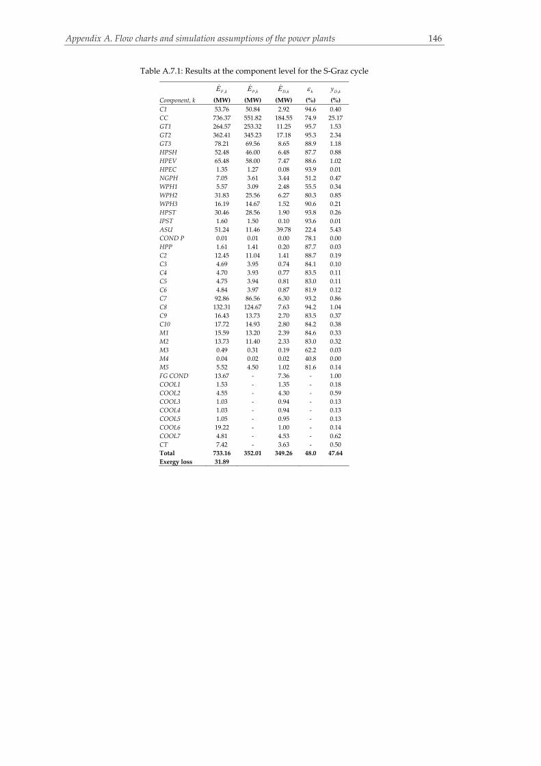
Appendix A. Flow charts and simulation assumptions of the power plants 146
Table A.7.1: Results at the component level for the S‐Graz cycle
,F kE ,P kE ,D kE k ,D ky
Component, k (MW) (MW) (MW) (%) (%)
C1 53.76 50.84 2.92 94.6 0.40
CC 736.37 551.82 184.55 74.9 25.17
GT1 264.57 253.32 11.25 95.7 1.53
GT2 362.41 345.23 17.18 95.3 2.34
GT3 78.21 69.56 8.65 88.9 1.18
HPSH 52.48 46.00 6.48 87.7 0.88
HPEV 65.48 58.00 7.47 88.6 1.02
HPEC 1.35 1.27 0.08 93.9 0.01
NGPH 7.05 3.61 3.44 51.2 0.47
WPH1 5.57 3.09 2.48 55.5 0.34
WPH2 31.83 25.56 6.27 80.3 0.85
WPH3 16.19 14.67 1.52 90.6 0.21
HPST 30.46 28.56 1.90 93.8 0.26
IPST 1.60 1.50 0.10 93.6 0.01
ASU 51.24 11.46 39.78 22.4 5.43
COND P 0.01 0.01 0.00 78.1 0.00
HPP 1.61 1.41 0.20 87.7 0.03
C2 12.45 11.04 1.41 88.7 0.19
C3 4.69 3.95 0.74 84.1 0.10
C4 4.70 3.93 0.77 83.5 0.11
C5 4.75 3.94 0.81 83.0 0.11
C6 4.84 3.97 0.87 81.9 0.12
C7 92.86 86.56 6.30 93.2 0.86
C8 132.31 124.67 7.63 94.2 1.04
C9 16.43 13.73 2.70 83.5 0.37
C10 17.72 14.93 2.80 84.2 0.38
M1 15.59 13.20 2.39 84.6 0.33
M2 13.73 11.40 2.33 83.0 0.32
M3 0.49 0.31 0.19 62.2 0.03
M4 0.04 0.02 0.02 40.8 0.00
M5 5.52 4.50 1.02 81.6 0.14
FG COND 13.67 ‐ 7.36 ‐ 1.00
COOL1 1.53 ‐ 1.35 ‐ 0.18
COOL2 4.55 ‐ 4.30 ‐ 0.59
COOL3 1.03 ‐ 0.94 ‐ 0.13
COOL4 1.03 ‐ 0.94 ‐ 0.13
COOL5 1.05 ‐ 0.95 ‐ 0.13
COOL6 19.22 ‐ 1.00 ‐ 0.14
COOL7 4.81 ‐ 4.53 ‐ 0.62
CT 7.42 ‐ 3.63 ‐ 0.50
Total 733.16 352.01 349.26 48.0 47.64
Exergy loss 31.89
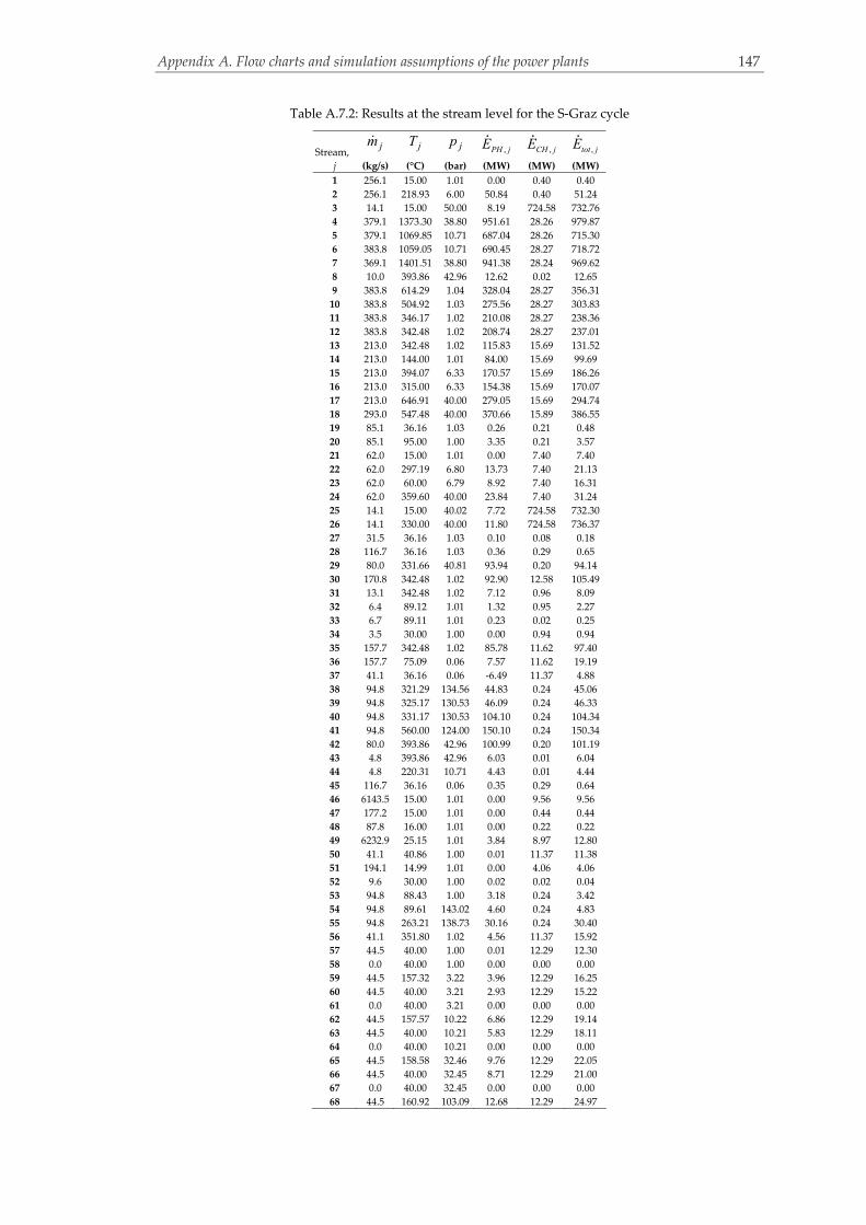
Appendix A. Flow charts and simulation assumptions of the power plants 147
Table A.7.2: Results at the stream level for the S‐Graz cycle
Stream, jm jT jp
,PH jE ,CH jE ,tot jE
j (kg/s) (°C) (bar) (MW) (MW) (MW)
1 256.1 15.00 1.01 0.00 0.40 0.40
2 256.1 218.93 6.00 50.84 0.40 51.24
3 14.1 15.00 50.00 8.19 724.58 732.76
4 379.1 1373.30 38.80 951.61 28.26 979.87
5 379.1 1069.85 10.71 687.04 28.26 715.30
6 383.8 1059.05 10.71 690.45 28.27 718.72
7 369.1 1401.51 38.80 941.38 28.24 969.62
8 10.0 393.86 42.96 12.62 0.02 12.65
9 383.8 614.29 1.04 328.04 28.27 356.31
10 383.8 504.92 1.03 275.56 28.27 303.83
11 383.8 346.17 1.02 210.08 28.27 238.36
12 383.8 342.48 1.02 208.74 28.27 237.01
13 213.0 342.48 1.02 115.83 15.69 131.52
14 213.0 144.00 1.01 84.00 15.69 99.69
15 213.0 394.07 6.33 170.57 15.69 186.26
16 213.0 315.00 6.33 154.38 15.69 170.07
17 213.0 646.91 40.00 279.05 15.69 294.74
18 293.0 547.48 40.00 370.66 15.89 386.55
19 85.1 36.16 1.03 0.26 0.21 0.48
20 85.1 95.00 1.00 3.35 0.21 3.57
21 62.0 15.00 1.01 0.00 7.40 7.40
22 62.0 297.19 6.80 13.73 7.40 21.13
23 62.0 60.00 6.79 8.92 7.40 16.31
24 62.0 359.60 40.00 23.84 7.40 31.24
25 14.1 15.00 40.02 7.72 724.58 732.30
26 14.1 330.00 40.00 11.80 724.58 736.37
27 31.5 36.16 1.03 0.10 0.08 0.18
28 116.7 36.16 1.03 0.36 0.29 0.65
29 80.0 331.66 40.81 93.94 0.20 94.14
30 170.8 342.48 1.02 92.90 12.58 105.49
31 13.1 342.48 1.02 7.12 0.96 8.09
32 6.4 89.12 1.01 1.32 0.95 2.27
33 6.7 89.11 1.01 0.23 0.02 0.25
34 3.5 30.00 1.00 0.00 0.94 0.94
35 157.7 342.48 1.02 85.78 11.62 97.40
36 157.7 75.09 0.06 7.57 11.62 19.19
37 41.1 36.16 0.06 ‐6.49 11.37 4.88
38 94.8 321.29 134.56 44.83 0.24 45.06
39 94.8 325.17 130.53 46.09 0.24 46.33
40 94.8 331.17 130.53 104.10 0.24 104.34
41 94.8 560.00 124.00 150.10 0.24 150.34
42 80.0 393.86 42.96 100.99 0.20 101.19
43 4.8 393.86 42.96 6.03 0.01 6.04
44 4.8 220.31 10.71 4.43 0.01 4.44
45 116.7 36.16 0.06 0.35 0.29 0.64
46 6143.5 15.00 1.01 0.00 9.56 9.56
47 177.2 15.00 1.01 0.00 0.44 0.44
48 87.8 16.00 1.01 0.00 0.22 0.22
49 6232.9 25.15 1.01 3.84 8.97 12.80
50 41.1 40.86 1.00 0.01 11.37 11.38
51 194.1 14.99 1.01 0.00 4.06 4.06
52 9.6 30.00 1.00 0.02 0.02 0.04
53 94.8 88.43 1.00 3.18 0.24 3.42
54 94.8 89.61 143.02 4.60 0.24 4.83
55 94.8 263.21 138.73 30.16 0.24 30.40
56 41.1 351.80 1.02 4.56 11.37 15.92
57 44.5 40.00 1.00 0.01 12.29 12.30
58 0.0 40.00 1.00 0.00 0.00 0.00
59 44.5 157.32 3.22 3.96 12.29 16.25
60 44.5 40.00 3.21 2.93 12.29 15.22
61 0.0 40.00 3.21 0.00 0.00 0.00
62 44.5 157.57 10.22 6.86 12.29 19.14
63 44.5 40.00 10.21 5.83 12.29 18.11
64 0.0 40.00 10.21 0.00 0.00 0.00
65 44.5 158.58 32.46 9.76 12.29 22.05
66 44.5 40.00 32.45 8.71 12.29 21.00
67 0.0 40.00 32.45 0.00 0.00 0.00
68 44.5 160.92 103.09 12.68 12.29 24.97

Appendix A. Flow charts and simulation assumptions of the power plants 148
69 44.5 30.00 103.09 11.56 12.31 23.86
70 0.0 30.00 103.09 0.00 0.00 0.00
71 8776.5 16.00 1.01 0.06 21.92 21.99
72 8776.5 16.00 1.37 0.38 21.92 22.30
73 329.1 16.00 1.37 0.01 0.82 0.84
74 329.1 26.00 1.33 0.29 0.82 1.11
75 551.0 26.00 1.33 0.49 1.38 1.87
76 221.9 26.00 1.33 0.20 0.55 0.75
77 221.9 16.00 1.37 0.01 0.55 0.56
78 8156.4 16.00 1.37 0.35 20.37 20.73
79 8447.4 16.00 1.37 0.37 21.10 21.47
80 291.0 16.00 1.37 0.01 0.73 0.74
81 291.0 26.00 1.33 0.26 0.73 0.99
82 7934.5 16.00 1.37 0.34 19.82 20.16
83 7473.0 16.00 1.37 0.32 18.67 18.99
84 7473.0 25.00 1.33 5.54 18.67 24.21
85 461.5 16.00 1.37 0.02 1.15 1.17
86 7764.0 25.04 1.33 5.80 19.39 25.19
87 8315.0 25.10 1.33 6.29 20.77 27.06
88 111.1 16.00 1.37 0.00 0.28 0.28
89 111.1 26.00 1.33 0.10 0.28 0.38
90 350.4 16.00 1.37 0.02 0.88 0.89
91 111.3 16.00 1.37 0.00 0.28 0.28
92 111.3 26.00 1.33 0.10 0.28 0.38
93 8426.1 25.11 1.33 6.38 21.05 27.43
94 239.1 16.00 1.37 0.01 0.60 0.61
95 113.6 16.00 1.37 0.00 0.28 0.29
96 113.6 26.00 1.33 0.10 0.28 0.38
97 8537.4 25.12 1.33 6.48 21.33 27.81
98 125.5 16.00 1.37 0.01 0.31 0.32
99 125.5 26.00 1.33 0.11 0.31 0.43
100 8651.0 25.14 1.33 6.58 21.61 28.19
101 8776.5 25.15 1.33 6.69 21.92 28.62
102 C7 92.18
103 C2 12.52
104 C3 4.64
105 C4 4.70
106 C5 4.68
107 C6 4.76
108 C1 53.76
109 C9 16.43
110 C10 17.72
111 P2 1.52
112 P1 0.01
113 C8 132.38
114 GT2 344.16
115 GT3 69.50
116 ST1 28.71
117 ST2 1.65
118 GT1 253.37
119 tot 352.07

Appendix A. Flow charts and simulation assumptions of the power plants 149
M
MM
M
MM
G
G
1011
1213
1517
18
2019 21 22
16
23
24
27
2932
14
33
3635
37
45
46
3034
31
80
72
69
89
82 81
75
76
71
6164
65
66
67
12
3
56
57
4
5
28
55
4847
49
125
70
51
62
78
8444
101
95
90
45
63
68
89
92
77
55
55
27
36
63
51
85
80
9741
54
43
43
44
3029
91
53
53
88
38 38
2626
4039
39
42
25
86
60
5957
7
79
58
Ch
imn
e
94
68
9
50
93
113
112
108 10
7
106
105
104
109
7374
103
102
100
99
87
118
114
117
116
115
120
119
83
98
110
111
C2
CO
OL1
C3
CO
OL2
C4
CT
LP
EC
LP
EV
LP
SH1
IPE
C
IPP
HPP
LP
P
De-
aera
tor
CO
ND
P
CO
ND
LP
ST
IPS
T1H
PST
GT
C1
GEN
1 RH
2
HPE
V
HP
EC
IPS
H
ST5
IPE
V
GEN
2
HP
SH
1H
PS
H2
IPS
T2
NG
PH
RH
1
SH
IFTE
R1
SH
IFTE
R2
LP
SH2
WP
H1
WP
H2
WP
H3
CO
OL
CAU
CA
U
ATR
Mix
CH
4/H
2O
CC
AP
H
Mix
CH
4/Ai
r
H2
PHC
5
MU
W P
CT
P
M4
M3
M5
M7
M2
M1
M8
M6
η: 4
8.5%
, ε: 4
6.5%
Wne
t: 33
9.8
MW
A.8: The ATR plant
Figure A.8.1: Structure of the ATR plant

Appendix A. Flow charts and simulation assumptions of the power plants 150
Table A.8.1: Results at the component level for the ATR plant
,F kE ,P kE ,D kE k ,D ky
Component, k (MW) (MW) (MW) (%) (%)
C1 221.95 211.43 10.53 95.3 1.44
CC 659.64 502.80 156.84 76.2 21.47
GT1 519.91 500.85 19.06 96.3 2.61
HPSH1 2.37 2.06 0.31 86.9 0.04
HPSH2 26.00 23.38 2.62 89.9 0.36
HPEV 36.90 32.76 4.14 88.8 0.57
HPEC 10.69 9.40 1.29 87.9 0.18
RH1 11.37 10.65 0.72 93.7 0.10
RH2 8.76 7.95 0.81 90.8 0.11
IPSH 5.51 4.72 0.79 85.6 0.11
IPEV 30.37 26.75 3.62 88.1 0.50
IPEC 6.89 5.75 1.14 83.5 0.16
LPSH1 1.54 1.14 0.40 74.1 0.05
LPSH2 3.37 2.86 0.52 84.7 0.07
LPEV 19.39 15.73 3.66 81.1 0.50
LPEC 13.01 8.44 4.57 64.9 0.63
NGPH 34.36 30.19 4.17 87.9 0.57
H2 PH 32.61 25.32 7.30 77.6 1.00
APH 9.38 5.91 3.47 63.0 0.47
WPH1 3.05 2.69 0.36 88.1 0.05
WPH2 10.38 9.53 0.86 91.7 0.12
WPH3 1.26 1.10 0.16 87.2 0.02
HPST 19.56 18.30 1.26 93.6 0.17
IPST1 19.98 18.91 1.07 94.6 0.15
IPST2 15.88 14.64 1.24 92.2 0.17
LPST 23.85 20.61 3.24 86.4 0.44
ST5 11.30 9.91 1.39 87.7 0.19
ATR 809.32 ‐ 51.81 ‐ 7.09
SHIFTER1 690.54 ‐ 3.43 ‐ 0.47
SHIFTER2 659.61 ‐ 0.63 ‐ 0.09
CAU 33.54 ‐ 29.95 ‐ 4.10
COND P 0.04 0.03 0.01 77.5 0.00
HPP 1.05 0.89 0.17 84.3 0.02
IPP 0.18 0.14 0.04 77.8 0.01
LPP 0.05 0.01 0.03 28.9 0.00
MUW P 0.01 0.01 0.00 68.0 0.00
C2 10.21 9.84 0.37 96.4 0.05
C3 2.70 2.21 0.48 82.0 0.07
C4 2.87 2.33 0.54 81.2 0.07
C5 4.34 3.58 0.76 82.4 0.10
De‐aerator 0.65 0.62 0.03 95.7 0.00
M1 0.17 0.16 0.01 95.9 0.00
M2 0.23 0.23 0.00 99.4 0.00
M4 1.79 1.78 0.01 99.2 0.00
M5 2.11 2.11 0.00 100.0 0.00
M6 1.01 0.95 0.06 94.1 0.01
M7 0.31 0.27 0.03 88.9 0.00
M8 0.08 0.04 0.05 43.0 0.01
Mix CH4/Air 428.31 419.98 8.33 98.1 1.14
Mix CH4/H2O 507.54 500.94 6.60 98.7 0.90
COOL CAU 13.71 ‐ 12.63 ‐ 1.73
COOL1 0.73 ‐ 0.67 ‐ 0.09
COOL2 0.62 ‐ 0.56 ‐ 0.08
COND 5.17 ‐ 3.85 ‐ 0.53
CT 2.50 ‐ 1.48 ‐ 0.20
Total 730.62 339.81 358.06 46.5 49.01
Exergy loss 32.75

Appendix A. Flow charts and simulation assumptions of the power plants 151
Table A.8.2: Results at the stream level for the ATR plant
Stream,
jm jT jp ,PH jE ,CH jE ,tot jE
j (kg/s) (°C) (bar) (MW) (MW) (MW)
1 590.89 15.00 1.01 0.00 0.92 0.92
2 590.89 375.07 15.46 211.43 0.92 212.35
3 14.00 15.00 50.00 8.15 721.47 729.62
4 588.87 1250.87 16.49 701.33 1.78 703.11
5 588.87 577.02 1.11 181.42 1.78 183.19
6 178.87 562.53 1.06 52.24 0.54 52.78
7 178.87 498.89 1.05 43.48 0.54 44.02
8 410.00 562.53 1.06 119.78 1.24 121.02
9 410.00 479.33 1.05 93.78 1.24 95.02
10 588.87 485.28 1.05 137.25 1.78 139.03
11 588.87 395.77 1.05 100.35 1.78 102.13
12 588.87 367.81 1.05 89.66 1.78 91.43
13 588.87 352.91 1.05 84.14 1.78 85.92
14 588.87 263.09 1.04 53.77 1.78 55.55
15 588.87 240.05 1.04 46.88 1.78 48.66
16 588.87 234.70 1.04 45.34 1.78 47.11
17 588.87 158.26 1.03 25.95 1.78 27.72
18 588.87 83.81 1.03 12.94 1.78 14.72
19 112.53 142.17 3.84 10.41 0.28 10.69
20 89.32 142.17 3.84 8.26 0.22 8.48
21 34.11 142.17 3.84 3.15 0.09 3.24
22 34.11 142.74 39.68 3.30 0.09 3.38
23 34.11 242.09 38.49 9.05 0.09 9.13
24 34.11 248.09 38.49 35.80 0.09 35.89
25 34.11 347.81 36.57 40.52 0.09 40.61
26 78.85 352.99 36.57 94.21 0.20 94.41
27 78.85 532.53 33.00 112.81 0.20 113.01
28 17.69 60.00 13.20 0.26 0.04 0.30
29 22.26 220.05 4.32 18.30 0.06 18.35
30 22.26 148.26 4.54 17.16 0.06 17.21
31 0.95 148.26 4.54 0.74 0.00 0.74
32 23.21 142.17 3.84 2.15 0.06 2.20
33 23.21 142.56 4.54 2.16 0.06 2.22
34 23.21 148.26 4.54 17.89 0.06 17.95
35 55.21 142.17 3.84 5.11 0.14 5.24
36 55.21 144.16 146.05 5.99 0.14 6.13
37 55.21 329.19 137.40 27.61 0.14 27.74
38 55.21 335.19 137.40 60.37 0.14 60.51
39 55.21 542.53 124.00 85.81 0.14 85.94
40 55.21 356.97 36.57 66.25 0.14 66.39
41 30.28 228.43 4.32 25.12 0.08 25.19
42 30.28 331.00 4.10 27.97 0.08 28.05
43 30.28 32.88 0.05 4.12 0.08 4.20
44 3078.21 16.00 1.37 0.13 7.69 7.82
45 3078.21 22.88 1.33 1.46 7.69 9.15
46 80.52 32.88 0.05 0.17 0.20 0.37
47 31.05 15.00 1.01 0.00 0.08 0.08
48 31.05 15.02 4.08 0.01 0.08 0.09
49 111.57 27.92 4.08 0.17 0.28 0.44
50 80.52 32.90 4.08 0.20 0.20 0.41
51 105.94 350.00 14.06 66.40 624.13 690.54
52 55.21 268.18 141.65 18.21 0.14 18.34
53 78.85 457.45 34.74 104.86 0.20 105.06
54 39.77 251.79 4.32 33.83 0.10 33.93
55 31.05 411.52 15.00 36.56 0.08 36.64
56 60.89 375.07 15.46 21.79 0.09 21.88
57 60.89 530.00 14.69 27.70 0.09 27.79
58 14.00 15.00 15.00 5.63 721.47 727.11
59 45.05 297.03 15.00 38.14 721.51 759.66
60 105.94 640.00 14.67 92.02 717.30 809.32
61 105.94 850.00 14.09 133.33 624.18 757.51
62 105.94 619.43 14.07 99.01 624.13 723.15
63 55.21 178.15 141.67 8.68 0.14 8.82
64 105.94 470.24 13.63 76.00 611.10 687.10
65 105.94 200.00 13.62 48.51 611.10 659.61
66 105.94 212.43 13.21 48.67 610.31 658.98
67 105.94 170.00 13.20 45.62 610.31 655.93
68 105.94 150.00 13.20 44.36 610.31 654.67

Appendix A. Flow charts and simulation assumptions of the power plants 152
69 88.25 60.00 13.20 30.39 610.27 640.65
70 58.87 63.12 12.94 26.00 604.75 630.75
71 58.87 510.46 17.00 54.89 604.75 659.64
72 1088.22 31.23 14.00 3.42 2.72 6.14
73 3363.76 15.00 1.01 0.00 5.24 5.24
74 90.98 15.00 1.01 0.00 0.23 0.23
75 48.05 16.00 1.01 0.00 0.12 0.12
76 3406.68 23.64 1.01 1.46 4.89 6.36
77 105.94 372.99 13.63 64.63 611.10 675.73
78 105.94 318.25 13.62 58.89 611.10 669.99
79 530.00 392.88 17.00 199.48 0.82 200.31
80 111.57 137.89 3.84 9.70 0.28 9.98
81 1552.28 16.00 1.37 0.07 3.88 3.94
82 1552.28 25.00 1.33 1.15 3.88 5.03
83 105.94 385.00 14.69 61.83 717.30 779.12
84 111.57 130.00 3.96 8.60 0.28 8.88
85 58.87 97.75 17.08 29.57 604.75 634.32
86 47.80 411.52 15.00 56.27 0.12 56.39
87 39.77 20.09 0.05 0.00 0.10 0.10
88 55.21 338.32 130.53 62.43 0.14 62.56
89 30.28 331.00 4.10 27.97 0.08 28.05
90 8.03 251.79 4.32 6.83 0.02 6.85
91 80.52 32.88 0.05 5.34 0.20 5.54
92 105.94 351.00 13.63 62.26 611.10 673.37
93 4805.37 16.00 1.37 0.21 12.00 12.21
94 530.00 375.07 15.46 189.64 0.82 190.47
95 44.74 356.97 36.57 53.69 0.11 53.80
96 10.46 356.97 36.57 12.56 0.03 12.58
97 10.46 32.88 0.05 1.26 0.03 1.29
98 50.24 32.88 0.05 1.22 0.13 1.35
99 39.77 251.43 4.10 33.56 0.10 33.66
100 0.00 331.00 4.10 0.00 0.00 0.00
101 39.77 20.00 4.10 0.02 0.10 0.12
102 39.77 251.43 4.10 33.56 0.10 33.66
103 1727.16 16.00 1.37 0.07 4.31 4.39
104 0.13 57.11 12.94 0.00 0.00 0.00
105 29.24 57.11 12.94 4.16 9.34 13.50
106 29.24 155.75 34.60 6.37 9.34 15.71
107 29.11 40.00 34.59 5.63 9.36 14.98
108 0.14 40.00 34.59 0.00 0.00 0.00
109 29.11 147.40 103.09 7.96 9.36 17.32
110 29.09 30.00 103.09 7.33 9.36 16.69
111 0.02 30.00 103.09 0.00 0.00 0.00
112 4805.37 23.64 1.33 2.71 12.00 14.71
113 4805.37 16.00 1.01 0.03 12.00 12.04
114 174.88 16.00 1.37 0.01 0.44 0.44
115 1643.63 25.00 1.33 1.22 4.11 5.32
116 91.35 25.00 1.33 0.07 0.23 0.30
117 91.35 16.00 1.37 0.00 0.23 0.23
118 83.53 16.00 1.37 0.00 0.21 0.21
119 83.53 25.00 1.33 0.06 0.21 0.27
120 1727.16 25.00 1.33 1.28 4.31 5.60
121 C1 221.95
122 ST1 18.30
123 ST2 18.91
124 ST3 14.64
125 ST4 20.61
126 COND P 0.04
127 LPP 0.05
128 IPP 0.18
129 HPP 1.05
130 C2 10.21
131 MUW P 0.01
132 C5 4.34
133 C3 2.70
134 C4 2.87
135 GT1 268.69
136 ST5 9.91
137 tot 339.81

Appendix A. Flow charts and simulation assumptions of the power plants 153
G
G
M
M
M
M
M
MG
9 10
11
12
13
14
15
17
52
54
20
19
21 22
18
23
24
27
28
29
32
16
40
39
41
33
36
35
37
38
42
43
45
44
46
30
34
25
26
31
48
47
7
6
53
55
56
57
58
60
91
82
69
70
72
74
83 8
4
75
85
86
87
88
89 90
76
73
77
79
80
64
66
81
78
65
59
61
63
92
93
94
10
8
96
95
98
99
10
01
01
10
2
10
31
04
10
51
06
49
10
7
63
MS
R-H
2
5
8
12
4
Ch
imn
ey
3
71
50
51
67
68
97
CT
P
CT
LPEC
LPEV
LPSH
IPECIP
PHP
P
LPP
De-a
era
tor
CO
ND
P
CO
ND
IPST
1HP
STNG
PH
GT1
C1
GEN
1
RH HPSH
HPEV
HPEC
IPSH
GT2
IPEV
GEN
2DB
IPST
2
CC
MUW
P
LPS
T
FG C
ON
D
C5
CO
OL
4C
OO
L3C
4C
OO
L2C
3C
OO
L1
C2
M4
M3
M2
M1
M5
η: 4
7.8%
, ε: 4
5.8%
Wne
t: 3
34.6
MW
A.9: The MSR plant
Figure A.9.1: Structure of the MSR plant
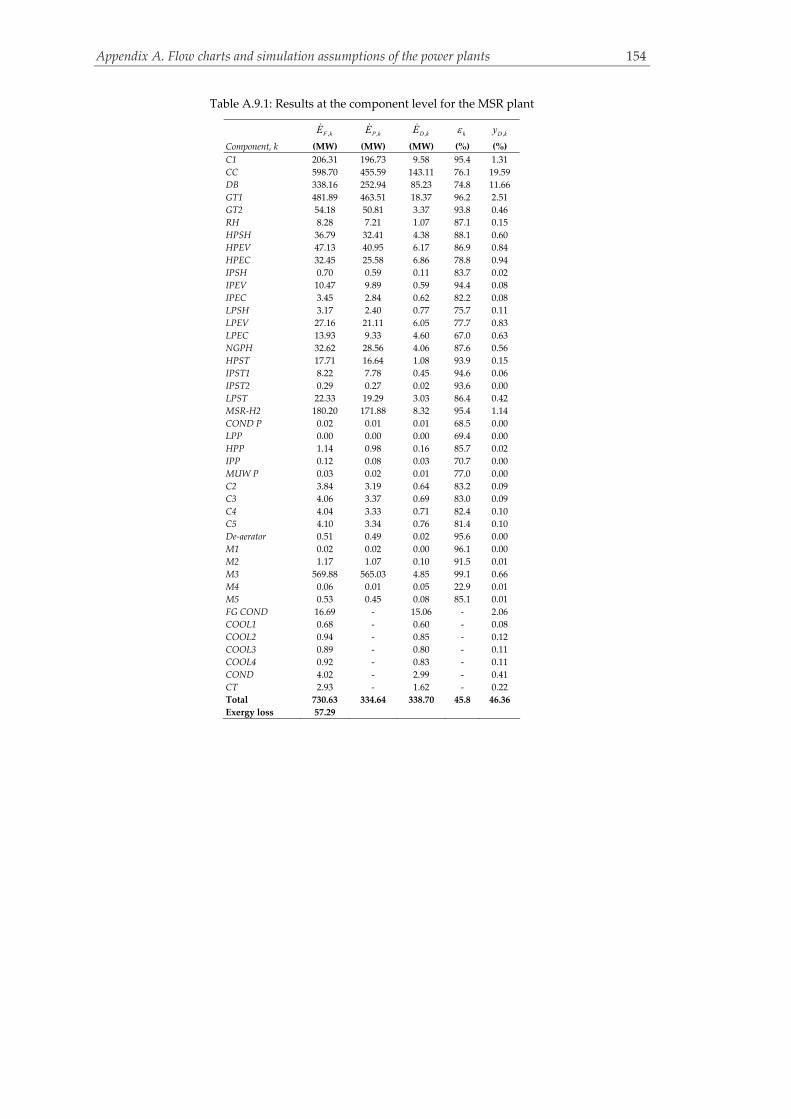
Appendix A. Flow charts and simulation assumptions of the power plants 154
Table A.9.1: Results at the component level for the MSR plant
,F kE ,P kE ,D kE k ,D ky
Component, k (MW) (MW) (MW) (%) (%)
C1 206.31 196.73 9.58 95.4 1.31
CC 598.70 455.59 143.11 76.1 19.59
DB 338.16 252.94 85.23 74.8 11.66
GT1 481.89 463.51 18.37 96.2 2.51
GT2 54.18 50.81 3.37 93.8 0.46
RH 8.28 7.21 1.07 87.1 0.15
HPSH 36.79 32.41 4.38 88.1 0.60
HPEV 47.13 40.95 6.17 86.9 0.84
HPEC 32.45 25.58 6.86 78.8 0.94
IPSH 0.70 0.59 0.11 83.7 0.02
IPEV 10.47 9.89 0.59 94.4 0.08
IPEC 3.45 2.84 0.62 82.2 0.08
LPSH 3.17 2.40 0.77 75.7 0.11
LPEV 27.16 21.11 6.05 77.7 0.83
LPEC 13.93 9.33 4.60 67.0 0.63
NGPH 32.62 28.56 4.06 87.6 0.56
HPST 17.71 16.64 1.08 93.9 0.15
IPST1 8.22 7.78 0.45 94.6 0.06
IPST2 0.29 0.27 0.02 93.6 0.00
LPST 22.33 19.29 3.03 86.4 0.42
MSR‐H2 180.20 171.88 8.32 95.4 1.14
COND P 0.02 0.01 0.01 68.5 0.00
LPP 0.00 0.00 0.00 69.4 0.00
HPP 1.14 0.98 0.16 85.7 0.02
IPP 0.12 0.08 0.03 70.7 0.00
MUW P 0.03 0.02 0.01 77.0 0.00
C2 3.84 3.19 0.64 83.2 0.09
C3 4.06 3.37 0.69 83.0 0.09
C4 4.04 3.33 0.71 82.4 0.10
C5 4.10 3.34 0.76 81.4 0.10
De‐aerator 0.51 0.49 0.02 95.6 0.00
M1 0.02 0.02 0.00 96.1 0.00
M2 1.17 1.07 0.10 91.5 0.01
M3 569.88 565.03 4.85 99.1 0.66
M4 0.06 0.01 0.05 22.9 0.01
M5 0.53 0.45 0.08 85.1 0.01
FG COND 16.69 ‐ 15.06 ‐ 2.06
COOL1 0.68 ‐ 0.60 ‐ 0.08
COOL2 0.94 ‐ 0.85 ‐ 0.12
COOL3 0.89 ‐ 0.80 ‐ 0.11
COOL4 0.92 ‐ 0.83 ‐ 0.11
COND 4.02 ‐ 2.99 ‐ 0.41
CT 2.93 ‐ 1.62 ‐ 0.22
Total 730.63 334.64 338.70 45.8 46.36
Exergy loss 57.29

Appendix A. Flow charts and simulation assumptions of the power plants 155
Table A.9.2: Results at the stream level for the MSR plant
Stream, jm jT jp
,PH jE ,CH jE ,tot jE
j (kg/s) (°C) (bar) (MW) (MW) (MW)
1 523.00 15.00 1.01 0.00 0.81 0.81
2 523.00 392.51 17.00 196.73 0.81 197.54
3 14.00 15.00 50.00 8.15 721.47 729.62
4 542.30 1230.15 16.49 652.06 1.07 653.13
5 542.30 567.08 1.11 170.17 1.07 171.25
6 553.20 994.77 1.10 422.50 1.69 424.18
7 553.20 674.76 1.06 242.30 1.69 243.98
8 553.20 609.47 1.06 209.68 1.69 211.37
9 553.20 592.38 1.06 201.40 1.69 203.09
10 553.20 513.25 1.05 164.61 1.69 166.30
11 553.20 401.68 1.05 117.48 1.69 119.17
12 553.20 314.01 1.04 85.04 1.69 86.72
13 553.20 311.97 1.04 84.34 1.69 86.02
14 553.20 280.43 1.04 73.86 1.69 75.55
15 553.20 269.55 1.04 70.41 1.69 72.09
16 553.20 259.32 1.04 67.23 1.69 68.92
17 553.20 156.38 1.03 40.07 1.69 41.76
18 553.20 72.68 1.03 26.14 1.69 27.82
19 111.13 139.81 3.60 9.93 0.28 10.21
20 79.81 139.81 3.60 7.13 0.20 7.33
21 12.89 139.81 3.60 1.15 0.03 1.18
22 12.89 140.86 57.12 1.24 0.03 1.27
23 12.89 264.43 55.40 4.07 0.03 4.11
24 12.89 270.43 55.40 13.96 0.03 13.99
25 12.89 294.01 52.63 14.55 0.03 14.58
26 23.81 347.74 52.63 28.84 0.06 28.90
27 23.81 559.47 50.00 36.05 0.06 36.10
28 0.83 217.70 4.10 0.67 0.00 0.68
29 30.57 249.55 4.10 25.74 0.08 25.82
30 30.57 146.37 4.32 23.34 0.08 23.42
31 0.75 146.37 4.32 0.58 0.00 0.58
32 31.32 139.81 3.60 2.80 0.08 2.88
33 31.32 139.82 4.32 2.80 0.08 2.88
34 31.32 146.37 4.32 23.92 0.08 24.00
35 66.92 139.81 3.60 5.98 0.17 6.15
36 66.92 141.54 134.56 6.96 0.17 7.13
37 66.92 325.17 130.53 32.54 0.17 32.71
38 66.92 331.17 130.53 73.50 0.17 73.67
39 66.92 559.38 124.00 105.91 0.17 106.08
40 10.92 422.41 52.63 14.39 0.03 14.41
41 31.40 248.71 4.10 26.42 0.08 26.50
42 0.00 32.88 0.05 0.00 0.00 0.00
43 31.40 32.88 0.05 4.09 0.08 4.17
44 2394.26 16.00 1.37 0.10 5.98 6.08
45 2394.26 22.88 1.33 1.14 5.98 7.12
46 31.40 32.88 0.05 0.07 0.08 0.15
47 0.83 392.96 17.00 0.97 0.00 0.97
48 56.00 422.41 52.63 73.81 0.14 73.95
49 4731.69 16.00 1.37 0.21 11.82 12.02
50 78.98 15.00 1.01 0.00 0.20 0.20
51 78.98 15.01 3.71 0.02 0.20 0.22
52 31.40 32.90 3.71 0.08 0.08 0.16
53 110.38 20.10 3.71 0.05 0.28 0.33
54 110.38 136.38 3.60 9.38 0.28 9.65
55 70.00 321.58 50.00 77.15 721.58 798.72
56 70.00 600.00 49.98 105.71 721.58 827.28
57 62.78 816.97 47.98 70.90 18.31 89.22
58 30.20 684.06 17.00 88.36 848.50 936.86
59 19.30 684.06 17.00 56.47 542.23 598.70
60 10.90 684.06 17.00 31.90 306.27 338.16
61 10.90 684.06 1.11 20.42 306.27 326.68
62 70.00 600.00 47.98 112.27 861.61 973.88
63 22.98 392.96 17.00 26.85 0.06 26.91
64 62.78 288.45 1.02 16.73 18.31 35.04
65 24.02 25.00 1.01 0.02 0.06 0.08
66 38.75 25.00 1.01 0.02 18.25 18.27
67 24.02 25.00 1.01 0.02 0.06 0.08
68 38.75 25.00 1.01 0.02 18.25 18.27

Appendix A. Flow charts and simulation assumptions of the power plants 156
69 38.75 131.81 3.22 3.21 18.25 21.47
70 0.14 40.00 3.21 0.00 0.00 0.00
71 38.61 40.00 3.21 2.54 18.25 20.79
72 38.61 151.95 10.22 5.91 18.25 24.16
73 0.26 40.00 10.21 0.00 0.00 0.00
74 38.36 40.00 10.21 4.96 18.26 23.22
75 38.36 152.83 32.46 8.29 18.26 26.55
76 0.08 40.00 32.45 0.00 0.00 0.00
77 38.28 40.00 32.45 7.39 18.27 25.66
78 38.28 154.99 103.09 10.73 18.27 29.00
79 0.03 30.00 103.09 0.00 0.00 0.00
80 38.25 30.00 103.09 9.80 18.28 28.08
81 1932.57 16.00 1.37 0.08 4.83 4.91
82 1932.57 26.00 1.33 1.72 4.83 6.54
83 86.75 26.00 1.33 0.08 0.22 0.29
84 86.75 16.00 1.37 0.00 0.22 0.22
85 111.06 26.00 1.33 0.10 0.28 0.38
86 111.06 16.00 1.37 0.00 0.28 0.28
87 100.23 26.00 1.33 0.09 0.25 0.34
88 100.23 16.00 1.37 0.00 0.25 0.25
89 106.82 26.00 1.33 0.09 0.27 0.36
90 106.82 16.00 1.37 0.00 0.27 0.27
91 419.00 392.51 17.00 157.61 0.65 158.26
92 438.30 1392.45 16.49 624.23 1.04 625.27
93 104.00 392.51 17.00 39.12 0.16 39.28
94 104.00 392.51 16.49 38.86 0.16 39.02
95 3312.18 15.00 1.01 0.00 5.16 5.16
96 92.58 15.00 1.01 0.00 0.23 0.23
97 47.32 16.00 1.01 0.00 0.12 0.12
98 3357.45 24.42 1.01 1.75 4.83 6.57
99 2337.43 26.00 1.33 2.08 5.84 7.92
100 2230.61 26.00 1.33 1.98 5.57 7.55
101 2130.38 26.00 1.33 1.89 5.32 7.21
102 2019.32 26.00 1.33 1.79 5.04 6.84
103 4326.83 16.00 1.37 0.19 10.81 11.00
104 4413.58 16.00 1.37 0.19 11.02 11.22
105 4524.64 16.00 1.37 0.20 11.30 11.50
106 4624.87 16.00 1.37 0.20 11.55 11.75
107 4731.69 16.00 1.01 0.03 11.82 11.85
108 4731.69 24.42 1.33 3.13 11.82 14.95
109 C1 206.31
110 ST1 16.67
111 ST2 7.80
112 ST3 0.29
113 ST4 19.33
114 COND P 0.02
115 LPP 0.00
116 HPP 1.15
117 IPP 0.12
118 GT1 256.99
119 GT2 50.81
120 MUW P 0.03
121 C2 3.84
122 C3 4.06
123 C4 4.04
124 C5 4.10
125 tot 334.53

Appendix A. Flow charts and simulation assumptions of the power plants 157
M
M
M
GG
M
M
34
5
7
8
9 10 11 12
13
1517
18
20
19
21
22
16
23
24
27
28
29
32
14
40
39
41
33
3635
37
38
42 43
45 44
46
30
34
25
26
31
52
47
2
58
53
54
10
5
100
101
148
4950
51
59
107
108
109
110
6
6061
62
6364
65
66
67
68
69
70 71
737274 75
7776
79
78
5556
9392
9190
8483
8285
81
80
94
97
98
9695
99
86
88
89
10
2
10
6
10
41
03
87
28
89
11
1
FG C
ON
D
C2
CO
OL
1C
3C
OO
L2
C4
CO
OL
3C
5C
OO
L4
CT
P
CT
LPE
C
LPEV
LPS
H
IPE
C
IPP
HPP
LPP
De-
aera
tor
CO
ND
P
CO
ND
LPS
TIP
ST
HP
ST
NG
PH
C1
GE
N1
RH
HP
SH
HP
EV
HP
EC
IPS
HIP
EV
GE
N2
C8
C9
C6
C7
CC
ST4
AS
U
M4
M3
M2
M1
CO
OL
5
CO
OL
6
GT
η: 4
4.8%
, ε: 4
2.7%
Wne
t: 31
3.4
MW
A.10: The simple oxy‐fuel plant
Figure A.10.1: Structure of the simple oxy‐fuel plant

Appendix A. Flow charts and simulation assumptions of the power plants 158
Table A.10.1: Results at the component level for the simple oxy‐fuel plant
,F kE ,P kE ,D kE k ,D ky
Component, k (MW) (MW) (MW) (%) (%)
C1 56.60 53.53 3.07 94.6 0.42
CC 733.81 512.57 221.24 69.9 30.18
GT 437.91 420.80 17.11 96.1 2.33
HPSH 41.65 35.88 5.78 86.1 0.79
HPEV 51.98 45.21 6.78 87.0 0.92
HPEC 33.59 28.22 5.37 84.0 0.73
RH 22.83 18.78 4.05 82.3 0.55
IPSH 0.10 0.06 0.04 61.4 0.01
IPEV 4.45 4.20 0.25 94.4 0.03
IPEC 0.77 0.65 0.13 83.7 0.02
LPSH 0.85 0.62 0.23 72.9 0.03
LPEV 12.43 10.24 2.20 82.3 0.30
LPEC 10.23 7.73 2.50 75.6 0.34
NGPH 3.56 1.04 2.52 29.3 0.34
HPST 35.41 33.02 2.39 93.2 0.33
IPST 28.63 26.97 1.66 94.2 0.23
LPST 51.25 44.29 6.96 86.4 0.95
ST4 21.91 19.22 2.69 87.7 0.37
ASU 53.95 11.59 42.36 21.5 5.78
COND P 0.04 0.03 0.01 78.5 0.00
LPP 0.00 0.00 0.00 64.3 0.00
HPP 1.25 1.08 0.17 86.1 0.02
IPP 0.02 0.01 0.01 63.9 0.00
C2 4.82 4.05 0.78 83.9 0.11
C3 4.80 4.01 0.79 83.5 0.11
C4 4.76 3.95 0.81 83.0 0.11
C5 4.83 3.96 0.87 82.1 0.12
C6 62.77 57.08 5.70 90.9 0.78
C7 56.67 54.82 1.85 96.7 0.25
C8 16.43 13.73 2.70 83.5 0.37
C9 17.89 15.08 2.81 84.3 0.38
De‐aerator 0.46 0.44 0.02 95.6 0.00
M1 0.65 0.61 0.04 93.1 0.01
M2 0.50 0.46 0.04 92.4 0.01
M3 0.17 0.17 0.00 100.0 0.00
M4 1.20 1.02 0.18 84.9 0.02
FG COND 9.39 ‐ 7.63 ‐ 1.04
COOL1 1.16 ‐ 1.03 ‐ 0.14
COOL2 1.14 ‐ 1.03 ‐ 0.14
COOL3 1.07 ‐ 0.97 ‐ 0.13
COOL4 1.10 ‐ 1.00 ‐ 0.14
COOL5 4.87 ‐ 4.59 ‐ 0.63
COOL6 17.07 ‐ 15.78 ‐ 2.15
COND 11.84 ‐ 8.81 ‐ 1.20
CT 6.62 ‐ 3.78 ‐ 0.51
Total 733.18 313.40 388.71 42.7 53.02
Exergy loss 31.08

Appendix A. Flow charts and simulation assumptions of the power plants 159
Table A.10.2: Results at the stream level for the simple oxy‐fuel plant
Stream, jm jT jp
,PH jE ,CH jE ,tot jE
j (kg/s) (°C) (bar) (MW) (MW) (MW)
1 269.63 15.00 1.01 0.00 0.42 0.42
2 62.00 362.30 40.00 23.94 7.40 31.33
3 14.06 15.00 50.00 8.19 724.58 732.76
4 14.06 200.00 49.99 9.70 724.58 734.27
5 14.06 200.00 40.00 9.23 724.58 733.81
6 382.00 190.05 40.00 95.67 102.82 198.49
7 458.06 1400.60 38.80 627.23 115.16 742.39
8 458.06 706.24 1.04 189.31 115.16 304.48
9 458.06 649.69 1.04 166.49 115.16 281.65
10 458.06 539.56 1.04 124.83 115.16 240.00
11 458.06 381.68 1.03 72.85 115.16 188.01
12 458.06 253.47 1.02 39.26 115.16 154.42
13 458.06 253.03 1.02 39.16 115.16 154.32
14 458.06 232.65 1.02 34.71 115.16 149.87
15 458.06 228.98 1.02 33.94 115.16 149.10
16 458.06 224.88 1.02 33.08 115.16 148.25
17 458.06 156.38 1.02 20.65 115.16 135.81
18 458.06 66.08 1.02 10.42 115.16 125.58
19 94.41 140.01 3.62 8.46 0.24 8.70
20 79.22 140.01 3.62 7.10 0.20 7.30
21 5.36 140.01 3.62 0.48 0.01 0.49
22 5.36 140.52 25.13 0.49 0.01 0.51
23 5.36 216.62 24.38 1.14 0.01 1.16
24 5.36 222.62 24.38 5.35 0.01 5.36
25 5.36 233.47 23.16 5.41 0.01 5.42
26 56.94 304.77 23.16 62.36 0.14 62.50
27 56.94 560.24 22.00 81.13 0.14 81.27
28 56.94 323.28 4.32 52.50 0.14 52.64
29 14.51 208.98 4.10 11.70 0.04 11.74
30 14.51 146.37 4.32 11.08 0.04 11.12
31 0.68 146.37 4.32 0.52 0.00 0.52
32 15.19 140.01 3.62 1.36 0.04 1.40
33 15.19 140.02 4.32 1.36 0.04 1.40
34 15.19 146.37 4.32 11.60 0.04 11.64
35 73.86 140.01 3.62 6.62 0.18 6.80
36 73.86 141.70 134.56 7.70 0.18 7.88
37 73.86 325.17 130.53 35.92 0.18 36.11
38 73.86 331.17 130.53 81.13 0.18 81.31
39 73.86 560.19 124.00 117.00 0.18 117.19
40 73.86 312.86 23.16 81.59 0.18 81.77
41 71.46 255.91 4.10 60.60 0.18 60.78
42 0.00 32.88 0.05 0.00 0.00 0.00
43 71.46 32.88 0.05 9.35 0.18 9.53
44 7048.82 16.00 1.37 0.31 17.61 17.91
45 7048.82 22.88 1.33 3.34 17.61 20.95
46 93.73 32.88 0.05 0.20 0.23 0.43
47 56.94 267.96 4.10 48.94 0.14 49.08
48 269.63 218.93 6.00 53.53 0.42 53.95
49 62.00 15.00 1.01 0.00 7.40 7.40
50 62.00 297.19 6.80 13.73 7.40 21.13
51 62.00 60.00 6.70 8.86 7.40 16.25
52 427.59 35.00 1.01 0.95 115.09 116.03
53 30.47 35.00 1.01 0.08 0.08 0.16
54 382.00 35.00 1.01 0.84 102.82 103.66
55 93.73 32.89 3.73 0.23 0.23 0.47
56 93.73 136.38 3.62 7.96 0.23 8.20
57 1851.17 16.00 1.37 0.08 4.62 4.70
58 207.63 15.00 1.01 0.00 4.19 4.19
59 45.59 35.00 1.01 0.10 12.27 12.37
60 45.59 150.46 3.22 4.15 12.27 16.42
61 44.93 40.00 3.21 2.99 12.27 15.26
62 0.66 40.00 3.21 0.00 0.00 0.00
63 44.93 157.80 10.22 7.00 12.27 19.27
64 44.62 40.00 10.21 5.85 12.28 18.12
65 0.31 40.00 10.21 0.00 0.00 0.00
66 44.62 158.62 32.46 9.80 12.28 22.08
67 44.53 40.00 32.45 8.71 12.29 21.00
68 0.09 40.00 32.45 0.00 0.00 0.00

Appendix A. Flow charts and simulation assumptions of the power plants 160
69 44.53 160.61 103.09 12.67 12.29 24.97
70 44.49 30.00 103.09 11.56 12.31 23.86
71 0.04 30.00 103.09 0.00 0.00 0.00
72 147.63 26.00 1.33 0.13 0.37 0.50
73 147.63 16.00 1.37 0.01 0.37 0.38
74 131.16 26.00 1.33 0.12 0.33 0.44
75 131.16 16.00 1.37 0.01 0.33 0.33
76 118.20 26.00 1.33 0.11 0.30 0.40
77 118.20 16.00 1.37 0.01 0.30 0.30
78 125.21 26.00 1.33 0.11 0.31 0.42
79 125.21 16.00 1.37 0.01 0.31 0.32
80 11504.08 16.00 1.01 506.75 28.74 535.48
81 11504.08 16.00 1.37 0.50 28.74 29.24
82 11378.87 16.00 1.37 0.49 28.42 28.92
83 11260.66 16.00 1.37 0.49 28.13 28.62
84 11129.50 16.00 1.37 0.48 27.80 28.28
85 10981.87 16.00 1.37 0.48 27.43 27.91
86 3933.05 16.00 1.37 0.17 9.82 10.00
87 1522.06 16.00 1.37 0.07 3.80 3.87
88 329.12 16.00 1.37 0.01 0.82 0.84
89 329.12 26.00 1.33 0.29 0.82 1.11
90 2410.99 26.00 1.33 2.14 6.02 8.16
91 2558.62 26.00 1.33 2.27 6.39 8.66
92 2689.78 26.00 1.33 2.39 6.72 9.11
93 2807.99 26.00 1.33 2.49 7.01 9.51
94 2933.20 26.00 1.33 2.61 7.33 9.93
95 8052.86 15.00 1.01 0.00 12.53 12.53
96 221.94 15.00 1.01 0.00 0.55 0.55
97 115.04 16.00 1.01 0.00 0.29 0.29
98 8159.75 24.09 1.01 3.92 11.73 15.65
99 11504.08 24.09 1.33 7.12 28.74 35.86
100 2081.87 16.00 1.37 0.09 5.20 5.29
101 2081.87 26.00 1.33 1.85 5.20 7.05
102 382.00 210.13 6.37 57.92 102.82 160.74
103 1522.06 26.00 1.33 1.35 3.80 5.15
104 4455.26 26.00 1.33 3.96 11.13 15.09
105 377.84 60.00 6.36 40.80 102.81 143.61
106 4.16 60.00 6.36 0.06 0.01 0.07
107 51.59 312.86 23.16 56.99 0.13 57.12
108 22.27 312.86 23.16 24.60 0.06 24.66
109 22.27 32.88 0.05 2.70 0.06 2.75
110 93.73 32.88 0.05 12.04 0.23 12.28
111 30.47 35.00 1.01 0.08 0.08 0.16
112 C1 56.15
113 C7 56.23
114 ST1 32.70
115 ST2 27.64
116 ST3 44.23
117 COND P 0.04
118 LPP 0.00
119 HPP 1.17
120 IPP 0.03
121 C6 62.28
122 C2 4.78
123 C3 4.76
124 C4 4.73
125 C5 4.79
126 GT1 299.14
127 C8 16.30
128 C9 17.75
129 ST4 19.07
130 tot 312.27

Appendix B. Assumptions used in the simulations and the conventional analyses
161
Appendix B
Assumptions used in the simulations and the
conventional analyses
B.1 Calculation of efficiencies and pressure drops for common components of the power plants
B.1.1 Compressors and expanders of GT systems (C1 and GT1) and CO2/H2O expanders (GT2)
The same polytropic efficiency has been assumed for C1, GT1 and GT2 (94% for the
compressor and 91% for the expanders).
Table B.1: Efficiencies of C1 and GT1 GT2 (all components have a mechanical efficiency of 99%)
Compressors (C1) a Expanders (GT1)a
ηpol (%) ηis (%) ηpol (%) ηis (%)
Base 94.0 91.5 Base 91.0 93.4
MEA‐0 94.0 91.5 MEA‐0 91.0 93.4
MEA‐0.2 94.0 91.5 MEA‐0.2 91.0 93.4
Simple oxy‐fuel 94.0 92.4 Simple oxy‐fuel 91.0 93.1
S‐Graz 94.0 92.4 S‐Graz
AZEP 85 94.0 91.5 GT1 91.0 92.0
AZEP 100 94.0 91.5 GT2 91.0 93.0
CLC 94.0 91.5 AZEP 85 91.0 93.5
MSR 94.0 91.6 AZEP 100 91.0 93.6
ATR CLC 91.0 93.6
C1 94.0 91.6 MSR 91.0 93.3
C2 94.0 93.9 ATR 91.0 93.5 a If not otherwise stated
B.1.2 Remaining compressors
The polytropic efficiencies of other types of compressors have been determined based on
their inlet volumetric flows and on whether or not they are centrifugal or axial. The CO2
compressors in all of the plants with CO2 capture, as well as fuel compressor (C5) in the ATR
plant, operating with lower mass flows and higher pressure ratios, have been assumed to be

Appendix B. Assumptions used in the simulations and the conventional analyses
162
Table B.2: Efficiencies of the remaining compressors and expanders of the plants (the ηmech of all
components is 99%)
Recycle compressors O2 compressors
ηpol (%) ηis (%) Vin (m3/s) ηpol (%)ηis (%)Vin (m3/s)
Simple oxy‐fuel Simple oxy‐fuel
C6 88.9 86.6 291.40 C8 77.1 71.2 45.00
C7 86.9 84.6 38.72 C9 75.4 69.5 7.80
S‐Graz S‐Graz
C7 89.1 86.8 345.55 C9 77.1 71.2 45.37
C8 87.6 85.0 77.61 C10 75.4 69.5 7.83
AZEP 85 (C6) 87.9 87.9 103.36 Fuel compressor
AZEP 100 (C6) 88.1 88.0 121.65 ATR (C5) 79.5 78.7 9.15
Flue gas compressor GT2
ηpol (%) ηis (%) Vin (m3/s) ηpol (%)ηis (%)
MEA‐0 (C2) 89.7 89.5 656.68 S‐Graz 91.0 90.0
MEA‐0.2 (C2) 89.7 89.5 656.68 AZEP 85 91.0 92.9
AZEP 100 91.0 92.9
CLC 91.0 93.0
MSR 91.0 93.8
CO2 compressors
ηpol (%) ηis (%) Vin (m3/s) ηpol (%)ηis (%)Vin (m3/s)
MEA‐0 AZEP 85
C3 80.3 78.1 20.66 C2 80.3 77.9 19.58
C4 79.1 76.7 6.21 C3 79.2 76.6 6.26
C5 78.0 75.6 1.92 C4 78.0 75.6 1.94
C6 76.9 74.1 0.60 C5 76.9 74.1 0.61
MEA‐0.2 AZEP 100
C3 80.5 78.3 25.43 C2 80.4 78.1 23.03
C4 79.2 76.7 6.22 C3 79.3 76.8 7.36
C5 78.0 75.6 1.92 C4 78.2 75.7 2.28
C6 76.9 74.1 0.60 C5 77.0 74.2 0.71
Simple oxyfuel CLC
C2 80.8 78.2 34.99 C2 80.4 79.2 22.72
C3 79.5 77.3 8.58 C3 79.3 78.0 7.26
C4 78.3 76.5 2.65 C4 78.2 77.7 2.25
C5 77.2 75.1 0.83 C5 77.0 76.9 0.70
S‐Graz MSR
C3 83.3 78.5 412.33 C2 80.4 78.2 22.32
C4 80.6 78.2 27.19 C3 79.3 76.9 7.33
C5 79.5 77.3 8.48 C4 78.2 76.0 2.27
C6 78.3 76.5 2.67 C5 77.0 74.4 0.71
C3 77.2 74.9 0.84 ATR
C3 76.7 74.5 0.50
C4 77.7 75.2 1.37
centrifugal and their efficiencies have been calculated using Equation B.1 (Ludwig, 2001). The
efficiencies of the remaining compressors have been calculated based on the calculation
method used for axial compressors. However, depending on the size and operation of the
compressors, their efficiencies have been adjusted analogously. Larger compressors, such as
the recycle compressors in the S‐Graz (C7 and C8) and the simple oxy‐fuel processes (C6 and
C7), as well as the flue gas compressor in the MEA plants (C2), have been assumed to be axial
with polytropic efficiencies of about 6 percentage points higher than that calculated for the
respective centrifugal compressors (Equation B.2). Oxygen compressors have also been
considered as axial compressors. However, due to higher risk that requires stronger
precaution measures, their efficiency has been estimated to be 10 percentage points lower
than the efficiency of the respective axial compressor (Equation B.3). Through the polytropic

Appendix B. Assumptions used in the simulations and the conventional analyses
163
efficiencies, the isentropic efficiencies have been calculated as a function of mass flows,
pressure ratios and compositions of the respective streams.
0.0098ln( ) 0.7736V , for centrifugal compressors (B.1)
0.0098ln( ) 0.8336V , for axial compressors (B.2)
0.0098ln( ) 0.7336V , for axial O2 compressors (B.3)
Here, V is the volumetric flow rate of the gas entering the compressor. The resulting
efficiencies for the remaining turbomachinery of the plants are shown in Table B.2 (Ludwig,
2001, Sinnott, 2005).
B.1.3 Steam turbines
The polytropic efficiencies of the high‐, intermediate‐ and low‐pressure steam turbines have
been assumed to be 90%, 92% and 87%, respectively. Due to the similar STs used in all of the
plants the isentropic efficiencies have been generalized for all processes: 91.6% for HPSTs,
93.3% for IPSTs and 88% for LPSTs and the additional ST4 of some plants.
B.1.4 Pumps
The isentropic efficiencies of the pumps have been calculated using Figure B.1, where the
behaviour of the total efficiency of pumps versus the mass flow rate of the component is
provided.
0
0,2
0,4
0,6
0,8
1
0 50 100 150 200 250 300
Figure B.1: Influence of mass flow on the pump efficiency (adopted from Peters, 2003)
The isentropic efficiency of the pumps has been calculated using Equation B.4 and assuming
a mechanical efficiency of 98%. The results of the calculations are shown in Table B.3.
mech is tot (B.4)
Efficiency, tot (‐)
Mass flow (kg/s)

Appendix B. Assumptions used in the simulations and the conventional analyses
164
Table B.3: Calculated efficiencies of pumps (the ηmech of all pumps is assumed to be 98%)
Mass flow rate ηtot ηis Win,motor ηmotor
(kg/s) (%) (%) (kW) (%)
Reference plant
COND P 94.6 89.9 91.7 45 87.2
HPP 65.2 86.5 88.2 1122 94.8
IPP 7.2 66.2 67.5 29 86.2
LPP 23.0 76.8 78.4 3 80.7
MEA‐0
COND P 94.5 89.9 91.7 45 87.2
HPP 65.4 86.5 88.3 1123 94.8
IPP 7.0 65.8 67.2 28 86.2
LPP 22.9 76.8 78.4 3 80.7
MEA‐0.2
COND P 94.5 90.0 91.7 45 87.2
HPP 65.4 86.5 88.3 1123 94.8
IPP 7.0 65.8 67.2 28 86.2
LPP 22.9 76.8 78.4 3 80.7
Simple oxy‐fuel
COND P 93.7 89.8 91.6 44 87.2
HPP 73.9 87.6 89.4 1255 95.1
IPP 5.3 63.3 64.6 22 85.6
LPP 15.2 73.0 74.5 2 79.9
S‐Graz
HPP 94.8 89.9 91.8 1648 95.7
LPP 116.7 91.8 93.7 15 84.7
AZEP 85
COND P 95.6 90.0 91.8 45 87.2
HPP 71.0 87.3 89.0 1207 95.0
IPP 6.2 64.7 66.1 26 85.9
LPP 18.5 74.9 76.4 2 80.3
AZEP 100
COND P 101.1 90.5 92.4 46 87.3
HPP 64.1 86.3 88.1 1100 94.7
IPP 15.5 73.2 74.7 58 87.8
LPP 20.4 75.8 77.3 3 80.5
CLC plant
COND P 93.3 89.8 91.6 43 87.1
HPP 68.1 86.9 88.6 979 94.5
IPP 14.0 72.3 73.8 51 87.6
LPP 20.8 75.9 77.5 3 80.5
MSR plant
COND P 31.3 79.7 81.3 16 84.8
HPP 67.4 86.8 88.5 1203 95.0
IPP 12.4 71.2 72.6 102 89.2
LPP 31.3 79.7 81.3 4 81.5
MUW P 79.0 88.2 90.0 32 86.4
ATR plant
COND P 80.5 88.4 90.2 43 87.1
HPP 55.3 84.9 86.7 1073 94.7
IPP 34.1 80.5 82.1 185 90.6
LPP 23.2 76.9 78.5 50 87.5
MUW P 31.1 79.6 81.2 15 84.6
B.1.5 Generators and motors
The electrical efficiencies of the generators have been kept constant and equal to 98.5%, while
the electrical efficiency of the motors follows the curve shown in Figure B.2.

Appendix B. Assumptions used in the simulations and the conventional analyses
165
0,4
0,6
0,8
1
0 1000 2000 3000 4000 5000 6000
Figure B.2: Influence of the capacity on the pump efficiency (adopted from Sinnott, 2005)
B.1.6 Heat exchangers
B.1.6.1 Pressure drops
The pressure drops in the HXs have been determined depending on the working fluid and
the temperature difference between the inlet and the outlet of this fluid. The pressure drop
has been set to 3% and 5% of the inlet pressure for water and steam streams, respectively. In
the evaporators, the pressure drops are handled by internal pumps. In gas/gas HXs, low‐
pressure and high‐pressure gases have been assumed to suffer by 0.6% and 0.65% pressure
drops per 100°C, respectively, always with respect to the inlet pressure.
For the HXs that constitute the HRSGs, the overall pressure drop of the hot side (HS, flue gas)
has been considered to be 30 mbar in all of the plants, with the exception of the S‐Graz cycle
that includes a single‐pressure level and has been assumed to have a pressure drop of 20
mbar (Ganapathy, 1991). These total pressure drops have been distributed among the HXs
depending on their heat transfer. The outlet pressure of the HRSG has been set to 1.028 bar,
assuming a 15 mbar pressure loss in the chimney.
The calculated pressure drop within each HX is provided in Table B.4.
Efficiency (‐)
Capacity (kW)
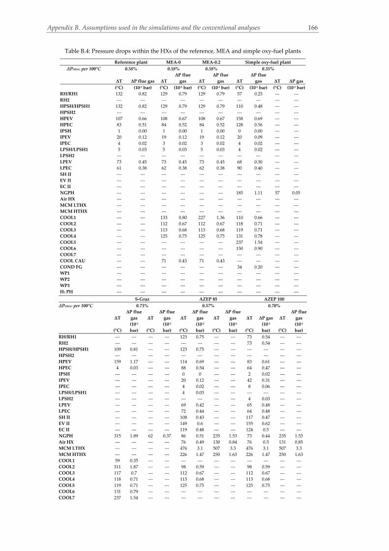
Appendix B. Assumptions used in the simulations and the conventional analyses
166
Table B.4: Pressure drops within the HXs of the reference, MEA and simple oxy‐fuel plants
Reference plant MEA‐0 MEA‐0.2 Simple oxy‐fuel plant
ΔPHRSG per 100°C 0.58% 0.58% 0.58% 0.35%
ΔT ΔP flue gas ΔT
ΔP flue
gas ΔT
ΔP flue
gas ΔT
ΔP flue
gas ΔT ΔP gas
(°C) (10‐2 bar) (°C) (10‐2 bar) (°C) (10‐2 bar) (°C) (10‐2 bar) (°C) (10‐2 bar)
RH/RH1 132 0.82 129 0.79 129 0.79 57 0.25 ‐‐‐ ‐‐‐
RH2 ‐‐‐ ‐‐‐ ‐‐‐ ‐‐‐ ‐‐‐ ‐‐‐ ‐‐‐ ‐‐‐ ‐‐‐ ‐‐‐
HPSH/HPSH1 132 0.82 129 0.79 129 0.79 110 0.48 ‐‐‐ ‐‐‐
HPSH2 ‐‐‐ ‐‐‐ ‐‐‐ ‐‐‐ ‐‐‐ ‐‐‐ ‐‐‐ ‐‐‐ ‐‐‐ ‐‐‐
HPEV 107 0.66 108 0.67 108 0.67 158 0.69 ‐‐‐ ‐‐‐
HPEC 83 0.51 84 0.52 84 0.52 128 0.56 ‐‐‐ ‐‐‐
IPSH 1 0.00 1 0.00 1 0.00 0 0.00 ‐‐‐ ‐‐‐
IPEV 20 0.12 19 0.12 19 0.12 20 0.09 ‐‐‐ ‐‐‐
IPEC 4 0.02 3 0.02 3 0.02 4 0.02 ‐‐‐ ‐‐‐
LPSH/LPSH1 5 0.03 5 0.03 5 0.03 4 0.02 ‐‐‐ ‐‐‐
LPSH2 ‐‐‐ ‐‐‐ ‐‐‐ ‐‐‐ ‐‐‐ ‐‐‐ ‐‐‐ ‐‐‐ ‐‐‐ ‐‐‐
LPEV 73 0.45 73 0.45 73 0.45 68 0.30 ‐‐‐ ‐‐‐
LPEC 61 0.38 62 0.38 62 0.38 90 0.40 ‐‐‐ ‐‐‐
SH II ‐‐‐ ‐‐‐ ‐‐‐ ‐‐‐ ‐‐‐ ‐‐‐ ‐‐‐ ‐‐‐ ‐‐‐ ‐‐‐
EV II ‐‐‐ ‐‐‐ ‐‐‐ ‐‐‐ ‐‐‐ ‐‐‐ ‐‐‐ ‐‐‐ ‐‐‐ ‐‐‐
EC II ‐‐‐ ‐‐‐ ‐‐‐ ‐‐‐ ‐‐‐ ‐‐‐ ‐‐‐ ‐‐‐ ‐‐‐ ‐‐‐
NGPH ‐‐‐ ‐‐‐ ‐‐‐ ‐‐‐ ‐‐‐ ‐‐‐ 185 1.11 57 0.05
Air HX ‐‐‐ ‐‐‐ ‐‐‐ ‐‐‐ ‐‐‐ ‐‐‐ ‐‐‐ ‐‐‐ ‐‐‐ ‐‐‐
MCM LTHX ‐‐‐ ‐‐‐ ‐‐‐ ‐‐‐ ‐‐‐ ‐‐‐ ‐‐‐ ‐‐‐ ‐‐‐ ‐‐‐
MCM HTHX ‐‐‐ ‐‐‐ ‐‐‐ ‐‐‐ ‐‐‐ ‐‐‐ ‐‐‐ ‐‐‐ ‐‐‐ ‐‐‐
COOL1 ‐‐‐ ‐‐‐ 133 0.80 227 1.36 110 0.66 ‐‐‐ ‐‐‐
COOL2 ‐‐‐ ‐‐‐ 112 0.67 112 0.67 118 0.71 ‐‐‐ ‐‐‐
COOL3 ‐‐‐ ‐‐‐ 113 0.68 113 0.68 119 0.71 ‐‐‐ ‐‐‐
COOL4 ‐‐‐ ‐‐‐ 125 0.75 125 0.75 131 0.78 ‐‐‐ ‐‐‐
COOL5 ‐‐‐ ‐‐‐ ‐‐‐ ‐‐‐ ‐‐‐ ‐‐‐ 237 1.54 ‐‐‐ ‐‐‐
COOL6 ‐‐‐ ‐‐‐ ‐‐‐ ‐‐‐ ‐‐‐ ‐‐‐ 150 0.90 ‐‐‐ ‐‐‐
COOL7 ‐‐‐ ‐‐‐ ‐‐‐ ‐‐‐ ‐‐‐ ‐‐‐ ‐‐‐ ‐‐‐ ‐‐‐ ‐‐‐
COOL CAU ‐‐‐ ‐‐‐ 71 0.43 71 0.43 ‐‐‐ ‐‐‐ ‐‐‐ ‐‐‐
COND FG ‐‐‐ ‐‐‐ ‐‐‐ ‐‐‐ ‐‐‐ ‐‐‐ 34 0.20 ‐‐‐ ‐‐‐
WP1 ‐‐‐ ‐‐‐ ‐‐‐ ‐‐‐ ‐‐‐ ‐‐‐ ‐‐‐ ‐‐‐ ‐‐‐ ‐‐‐
WP2 ‐‐‐ ‐‐‐ ‐‐‐ ‐‐‐ ‐‐‐ ‐‐‐ ‐‐‐ ‐‐‐ ‐‐‐ ‐‐‐
WP3 ‐‐‐ ‐‐‐ ‐‐‐ ‐‐‐ ‐‐‐ ‐‐‐ ‐‐‐ ‐‐‐ ‐‐‐ ‐‐‐
H2 PH ‐‐‐ ‐‐‐ ‐‐‐ ‐‐‐ ‐‐‐ ‐‐‐ ‐‐‐ ‐‐‐ ‐‐‐ ‐‐‐
S‐Graz AZEP 85 AZEP 100
ΔPHRSG per 100°C 0.73% 0.57% 0.70%
ΔT
ΔP flue
gas ΔT
ΔP flue
gas ΔT
ΔP flue
gas ΔT
ΔP flue
gas ΔT ΔP gas ΔT
ΔP flue
gas
(°C)
(10‐2
bar) (°C)
(10‐2
bar) (°C)
(10‐2
bar) (°C)
(10‐2
bar) (°C)
(10‐2
bar) (°C)
(10‐2
bar)
RH/RH1 ‐‐‐ ‐‐‐ ‐‐‐ ‐‐‐ 123 0.75 ‐‐‐ ‐‐‐ 73 0.54 ‐‐‐ ‐‐‐
RH2 ‐‐‐ ‐‐‐ ‐‐‐ ‐‐‐ ‐‐‐ ‐‐‐ ‐‐‐ ‐‐‐ 73 0.54 ‐‐‐ ‐‐‐
HPSH/HPSH1 109 0.81 ‐‐‐ ‐‐‐ 123 0.75 ‐‐‐ ‐‐‐ ‐‐‐ ‐‐‐ ‐‐‐ ‐‐‐
HPSH2 ‐‐‐ ‐‐‐ ‐‐‐ ‐‐‐ ‐‐‐ ‐‐‐ ‐‐‐ ‐‐‐ ‐‐‐ ‐‐‐ ‐‐‐ ‐‐‐
HPEV 159 1.17 ‐‐‐ ‐‐‐ 114 0.69 ‐‐‐ ‐‐‐ 83 0.61 ‐‐‐ ‐‐‐
HPEC 4 0.03 ‐‐‐ ‐‐‐ 88 0.54 ‐‐‐ ‐‐‐ 64 0.47 ‐‐‐ ‐‐‐
IPSH ‐‐‐ ‐‐‐ ‐‐‐ ‐‐‐ 0 0 ‐‐‐ ‐‐‐ 2 0.02 ‐‐‐ ‐‐‐
IPEV ‐‐‐ ‐‐‐ ‐‐‐ ‐‐‐ 20 0.12 ‐‐‐ ‐‐‐ 42 0.31 ‐‐‐ ‐‐‐
IPEC ‐‐‐ ‐‐‐ ‐‐‐ ‐‐‐ 4 0.02 ‐‐‐ ‐‐‐ 8 0.06 ‐‐‐ ‐‐‐
LPSH/LPSH1 ‐‐‐ ‐‐‐ ‐‐‐ ‐‐‐ 4 0.03 ‐‐‐ ‐‐‐ ‐‐‐ ‐‐‐ ‐‐‐ ‐‐‐
LPSH2 ‐‐‐ ‐‐‐ ‐‐‐ ‐‐‐ ‐‐‐ ‐‐‐ ‐‐‐ ‐‐‐ 4 0.03 ‐‐‐ ‐‐‐
LPEV ‐‐‐ ‐‐‐ ‐‐‐ ‐‐‐ 69 0.42 ‐‐‐ ‐‐‐ 65 0.48 ‐‐‐ ‐‐‐
LPEC ‐‐‐ ‐‐‐ ‐‐‐ ‐‐‐ 72 0.44 ‐‐‐ ‐‐‐ 64 0.48 ‐‐‐ ‐‐‐
SH II ‐‐‐ ‐‐‐ ‐‐‐ ‐‐‐ 108 0.43 ‐‐‐ ‐‐‐ 117 0.47 ‐‐‐ ‐‐‐
EV II ‐‐‐ ‐‐‐ ‐‐‐ ‐‐‐ 149 0.6 ‐‐‐ ‐‐‐ 155 0.62 ‐‐‐ ‐‐‐
EC II ‐‐‐ ‐‐‐ ‐‐‐ ‐‐‐ 119 0.48 ‐‐‐ ‐‐‐ 124 0.5 ‐‐‐ ‐‐‐
NGPH 315 1.89 62 0.37 86 0.51 235 1.53 73 0.44 235 1.53
Air HX ‐‐‐ ‐‐‐ ‐‐‐ ‐‐‐ 76 0.49 130 0.84 76 0.5 131 0.85
MCM LTHX ‐‐‐ ‐‐‐ ‐‐‐ ‐‐‐ 476 3.1 507 3.3 476 3.1 507 3.3
MCM HTHX ‐‐‐ ‐‐‐ ‐‐‐ ‐‐‐ 226 1.47 250 1.63 226 1.47 250 1.63
COOL1 59 0.35 ‐‐‐ ‐‐‐ ‐‐‐ ‐‐‐ ‐‐‐ ‐‐‐ ‐‐‐ ‐‐‐ ‐‐‐ ‐‐‐
COOL2 311 1.87 ‐‐‐ ‐‐‐ 98 0.59 ‐‐‐ ‐‐‐ 98 0.59 ‐‐‐ ‐‐‐
COOL3 117 0.7 ‐‐‐ ‐‐‐ 112 0.67 ‐‐‐ ‐‐‐ 112 0.67 ‐‐‐ ‐‐‐
COOL4 118 0.71 ‐‐‐ ‐‐‐ 113 0.68 ‐‐‐ ‐‐‐ 113 0.68 ‐‐‐ ‐‐‐
COOL5 119 0.71 ‐‐‐ ‐‐‐ 125 0.75 ‐‐‐ ‐‐‐ 125 0.75 ‐‐‐ ‐‐‐
COOL6 131 0.79 ‐‐‐ ‐‐‐ ‐‐‐ ‐‐‐ ‐‐‐ ‐‐‐ ‐‐‐ ‐‐‐ ‐‐‐ ‐‐‐
COOL7 237 1.54 ‐‐‐ ‐‐‐ ‐‐‐ ‐‐‐ ‐‐‐ ‐‐‐ ‐‐‐ ‐‐‐ ‐‐‐ ‐‐‐
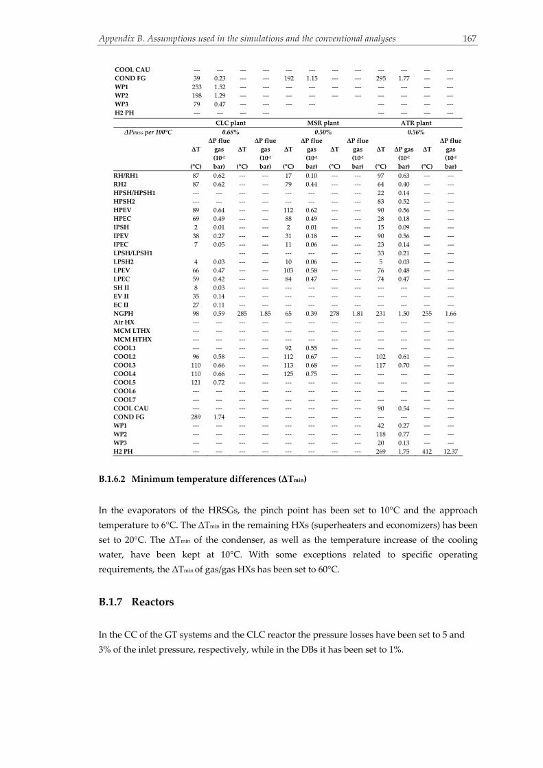
Appendix B. Assumptions used in the simulations and the conventional analyses
167
COOL CAU ‐‐‐ ‐‐‐ ‐‐‐ ‐‐‐ ‐‐‐ ‐‐‐ ‐‐‐ ‐‐‐ ‐‐‐ ‐‐‐ ‐‐‐ ‐‐‐
COND FG 39 0.23 ‐‐‐ ‐‐‐ 192 1.15 ‐‐‐ ‐‐‐ 295 1.77 ‐‐‐ ‐‐‐
WP1 253 1.52 ‐‐‐ ‐‐‐ ‐‐‐ ‐‐‐ ‐‐‐ ‐‐‐ ‐‐‐ ‐‐‐ ‐‐‐ ‐‐‐
WP2 198 1.29 ‐‐‐ ‐‐‐ ‐‐‐ ‐‐‐ ‐‐‐ ‐‐‐ ‐‐‐ ‐‐‐ ‐‐‐ ‐‐‐
WP3 79 0.47 ‐‐‐ ‐‐‐ ‐‐‐ ‐‐‐ ‐‐‐ ‐‐‐ ‐‐‐ ‐‐‐
H2 PH ‐‐‐ ‐‐‐ ‐‐‐ ‐‐‐ ‐‐‐ ‐‐‐ ‐‐‐ ‐‐‐
CLC plant MSR plant ATR plant
ΔPHRSG per 100°C 0.68% 0.50% 0.56%
ΔT
ΔP flue
gas ΔT
ΔP flue
gas ΔT
ΔP flue
gas ΔT
ΔP flue
gas ΔT ΔP gas ΔT
ΔP flue
gas
(°C)
(10‐2
bar) (°C)
(10‐2
bar) (°C)
(10‐2
bar) (°C)
(10‐2
bar) (°C)
(10‐2
bar) (°C)
(10‐2
bar)
RH/RH1 87 0.62 ‐‐‐ ‐‐‐ 17 0.10 ‐‐‐ ‐‐‐ 97 0.63 ‐‐‐ ‐‐‐
RH2 87 0.62 ‐‐‐ ‐‐‐ 79 0.44 ‐‐‐ ‐‐‐ 64 0.40 ‐‐‐ ‐‐‐
HPSH/HPSH1 ‐‐‐ ‐‐‐ ‐‐‐ ‐‐‐ ‐‐‐ ‐‐‐ ‐‐‐ ‐‐‐ 22 0.14 ‐‐‐ ‐‐‐
HPSH2 ‐‐‐ ‐‐‐ ‐‐‐ ‐‐‐ ‐‐‐ ‐‐‐ ‐‐‐ ‐‐‐ 83 0.52 ‐‐‐ ‐‐‐
HPEV 89 0.64 ‐‐‐ ‐‐‐ 112 0.62 ‐‐‐ ‐‐‐ 90 0.56 ‐‐‐ ‐‐‐
HPEC 69 0.49 ‐‐‐ ‐‐‐ 88 0.49 ‐‐‐ ‐‐‐ 28 0.18 ‐‐‐ ‐‐‐
IPSH 2 0.01 ‐‐‐ ‐‐‐ 2 0.01 ‐‐‐ ‐‐‐ 15 0.09 ‐‐‐ ‐‐‐
IPEV 38 0.27 ‐‐‐ ‐‐‐ 31 0.18 ‐‐‐ ‐‐‐ 90 0.56 ‐‐‐ ‐‐‐
IPEC 7 0.05 ‐‐‐ ‐‐‐ 11 0.06 ‐‐‐ ‐‐‐ 23 0.14 ‐‐‐ ‐‐‐
LPSH/LPSH1 ‐‐‐ ‐‐‐ ‐‐‐ ‐‐‐ ‐‐‐ ‐‐‐ 33 0.21 ‐‐‐ ‐‐‐
LPSH2 4 0.03 ‐‐‐ ‐‐‐ 10 0.06 ‐‐‐ ‐‐‐ 5 0.03 ‐‐‐ ‐‐‐
LPEV 66 0.47 ‐‐‐ ‐‐‐ 103 0.58 ‐‐‐ ‐‐‐ 76 0.48 ‐‐‐ ‐‐‐
LPEC 59 0.42 ‐‐‐ ‐‐‐ 84 0.47 ‐‐‐ ‐‐‐ 74 0.47 ‐‐‐ ‐‐‐
SH II 8 0.03 ‐‐‐ ‐‐‐ ‐‐‐ ‐‐‐ ‐‐‐ ‐‐‐ ‐‐‐ ‐‐‐ ‐‐‐ ‐‐‐
EV II 35 0.14 ‐‐‐ ‐‐‐ ‐‐‐ ‐‐‐ ‐‐‐ ‐‐‐ ‐‐‐ ‐‐‐ ‐‐‐ ‐‐‐
EC II 27 0.11 ‐‐‐ ‐‐‐ ‐‐‐ ‐‐‐ ‐‐‐ ‐‐‐ ‐‐‐ ‐‐‐ ‐‐‐ ‐‐‐
NGPH 98 0.59 285 1.85 65 0.39 278 1.81 231 1.50 255 1.66
Air HX ‐‐‐ ‐‐‐ ‐‐‐ ‐‐‐ ‐‐‐ ‐‐‐ ‐‐‐ ‐‐‐ ‐‐‐ ‐‐‐ ‐‐‐ ‐‐‐
MCM LTHX ‐‐‐ ‐‐‐ ‐‐‐ ‐‐‐ ‐‐‐ ‐‐‐ ‐‐‐ ‐‐‐ ‐‐‐ ‐‐‐ ‐‐‐ ‐‐‐
MCM HTHX ‐‐‐ ‐‐‐ ‐‐‐ ‐‐‐ ‐‐‐ ‐‐‐ ‐‐‐ ‐‐‐ ‐‐‐ ‐‐‐ ‐‐‐ ‐‐‐
COOL1 ‐‐‐ ‐‐‐ ‐‐‐ ‐‐‐ 92 0.55 ‐‐‐ ‐‐‐ ‐‐‐ ‐‐‐ ‐‐‐ ‐‐‐
COOL2 96 0.58 ‐‐‐ ‐‐‐ 112 0.67 ‐‐‐ ‐‐‐ 102 0.61 ‐‐‐ ‐‐‐
COOL3 110 0.66 ‐‐‐ ‐‐‐ 113 0.68 ‐‐‐ ‐‐‐ 117 0.70 ‐‐‐ ‐‐‐
COOL4 110 0.66 ‐‐‐ ‐‐‐ 125 0.75 ‐‐‐ ‐‐‐ ‐‐‐ ‐‐‐ ‐‐‐ ‐‐‐
COOL5 121 0.72 ‐‐‐ ‐‐‐ ‐‐‐ ‐‐‐ ‐‐‐ ‐‐‐ ‐‐‐ ‐‐‐ ‐‐‐ ‐‐‐
COOL6 ‐‐‐ ‐‐‐ ‐‐‐ ‐‐‐ ‐‐‐ ‐‐‐ ‐‐‐ ‐‐‐ ‐‐‐ ‐‐‐ ‐‐‐ ‐‐‐
COOL7 ‐‐‐ ‐‐‐ ‐‐‐ ‐‐‐ ‐‐‐ ‐‐‐ ‐‐‐ ‐‐‐ ‐‐‐ ‐‐‐ ‐‐‐ ‐‐‐
COOL CAU ‐‐‐ ‐‐‐ ‐‐‐ ‐‐‐ ‐‐‐ ‐‐‐ ‐‐‐ ‐‐‐ 90 0.54 ‐‐‐ ‐‐‐
COND FG 289 1.74 ‐‐‐ ‐‐‐ ‐‐‐ ‐‐‐ ‐‐‐ ‐‐‐ ‐‐‐ ‐‐‐ ‐‐‐ ‐‐‐
WP1 ‐‐‐ ‐‐‐ ‐‐‐ ‐‐‐ ‐‐‐ ‐‐‐ ‐‐‐ ‐‐‐ 42 0.27 ‐‐‐ ‐‐‐
WP2 ‐‐‐ ‐‐‐ ‐‐‐ ‐‐‐ ‐‐‐ ‐‐‐ ‐‐‐ ‐‐‐ 118 0.77 ‐‐‐ ‐‐‐
WP3 ‐‐‐ ‐‐‐ ‐‐‐ ‐‐‐ ‐‐‐ ‐‐‐ ‐‐‐ ‐‐‐ 20 0.13 ‐‐‐ ‐‐‐
H2 PH ‐‐‐ ‐‐‐ ‐‐‐ ‐‐‐ ‐‐‐ ‐‐‐ ‐‐‐ ‐‐‐ 269 1.75 412 12.37
B.1.6.2 Minimum temperature differences (ΔTmin)
In the evaporators of the HRSGs, the pinch point has been set to 10°C and the approach
temperature to 6°C. The ΔΤmin in the remaining HXs (superheaters and economizers) has been
set to 20°C. The ΔΤmin of the condenser, as well as the temperature increase of the cooling
water, have been kept at 10°C. With some exceptions related to specific operating
requirements, the ΔΤmin of gas/gas HXs has been set to 60°C.
B.1.7 Reactors
In the CC of the GT systems and the CLC reactor the pressure losses have been set to 5 and
3% of the inlet pressure, respectively, while in the DBs it has been set to 1%.

Appendix B. Assumptions used in the simulations and the conventional analyses
168
B.2 Application of the conventional exergy‐based methods
B.2.1 Application of the exergetic analysis
Matlab is the programming language used to perform the exergetic analysis. In Matlab,
exergy balances are stated both at the component level and for the overall plant, i.e., balances
regarding the rate of product exergy, the rate of fuel exergy and rate of exergy destruction for
each component and for the overall system. The statements of the exergy rates are carried out
based on the SPECO approach (Lazzaretto and Tsatsaronis, 2006). To calculate the (physical
and chemical) exergies of streams, in order to use them in the exergy balances of the analysis,
the software THESIS, originally developed at the RWTH Aachen, has been used. The main
thermodynamic values of the streams (mass flows, temperatures and pressures) and their
composition are exported from EbsilonProfessional using a .dll file and they are supplied as
input to the exergy calculation software. The respective enthalpies, entropies and exergy
values are then calculated. The number of the components and the streams included in each
plant are shown in Table B.5.
Table B.5: Power plant characteristics
Ref.
plant
Simple
oxy‐fuel
plant
S‐Graz
cycle
MEA
CLC
AZEP
100
AZEP
85 ATR
MSR‐
H2
Number of
streams
67 (10
shafts)
131 (19
shafts)
119 (18
shafts)
122 (17
shafts)
120 (16
shafts)
135 (17
shafts)
138 (17
shafts)
138 (17
shafts)
125 (17
shafts)
Number of
componentsa 26 45 40 40 42 48 48 55 43
of which
dissipative 2 9 9 8 7 7 7 9 7
a Not including valves, splitters, generators or motors
B.2.2 Application of the economic analysis
The main challenge in an analytical economic analysis is the estimation of the investment
costs of plant components, since most of the available cost sources refer to relatively small‐
scale facilities. These values are difficult to adjust when large equipment is considered. In this
thesis, various sources are combined and a large number of different data are used as
reference. The reference data used for all components, their design characteristics and their
sources are presented in Table B.6.
The size exponents have been used to extrapolate costs based on sizing parameters and
have been calculated through cost comparisons with equipment found in the references.
Temperatures, surface areas and heat transfer rates have also either been extracted from the
reports used (Tsatsaronis and Winhold, 1984; Buchanan et al., 2000; Tsatsaronis and Cziesla,
2002; Turton et al., 2002; Framer, 2006) or they have been calculated after simulations in
EbsilonProfessional. The modular factors shown in Table B.6 are used to convert PEC to FCI

Appendix B. Assumptions used in the simulations and the conventional analyses
169
and they have been derived from Buchanan et al. (2000) as a result of comparisons between
equipment and total costs of components.
To calculate a HX’s surface area, its overall heat transfer coefficient, Uo, must first be
estimated. Typical value ranges of the overall heat transfer coefficients for variant component
types can be found in literature (Naim Afgan et. al, 1996). Nonetheless, coefficient values are
spread over wide ranges, and usually a mean value is chosen. In this thesis, the heat transfer
coefficients have been calculated in detail, following the process described in Appendix C.
Construction materials are also important for cost calculations. However, at first, plant
components in this thesis are assumed to be constructed with similar materials as the
reference components. For high‐temperature HXs, where no real economic data have been
found, the materials have been assumed to be two to five times higher (depending on the
operating temperature) than the base cost of the most economical HX (economizer). A
detailed examination of different materials is performed in the LCA of the plants.
Because each part of the system (e.g., GT and ST systems) is simulated as a separate
component, a strategy to split the system costs had to be defined. For example, in the GT
system, 40% of the total cost is assumed to correspond to the expander, 35% to the
compressor and 25% to the CC. In the ST system, the cost is shared among the different
pressure‐level STs, based on their contribution to the overall power output of the ST system.
This is also in agreement with a general design assumption of the STs that lower pressure
requires larger shuffles, thus it is associated with costlier construction.
To extrapolate the cost of the GT systems of the plants with CO2 capture from the GT
system of the reference plant, the respective system components have been compared, based
on the power output (for the expander), the power input (for the compressor) and the mass
flow of the combustion products (for the CC). The cost of the additional ST (ST4) is calculated
based on the LPST of each plant, since the inlet and outlet pressures and temperatures of
these components are comparable.
The MCM reactor was initially regarded as one component for the cost calculations. The
costs of the included HXs and CC were calculated separately following the guidelines
described above. Finally, the cost of the MCM is calculated by subtracting the cost of the CC
and the HXs from the cost of the overall reactor.
In the CLC plant, the cost of the metal oxide has not been calculated because of high
uncertainty (Lyngfelt and Thunman, 2005). However, even at the highest suggested prices
and quantities it could be considered negligible in comparison to the total cost of the unit. The
installation and the metal oxide costs of the CLC unit have been considered to be 20% of the
equipment cost.
The cost of the CAU in MEA‐0.2 was calculated based on a predefined 50% overall
increase in the total FCI of the plant, when compared to the reference plant (IPCC report,
2005) and has then been split into its constitutive components: 55% absorber, 18%
regenerator, 27% remaining components (Abu‐Zahra et al., 2007). The extrapolation to MEA‐0
has been performed based on comparison between the size of the equipment used here and
that used in MEA‐0.2. The absorber is designed as a packed vessel. The height and diameter
of the absorption column have been estimated following calculations presented by Rubin and
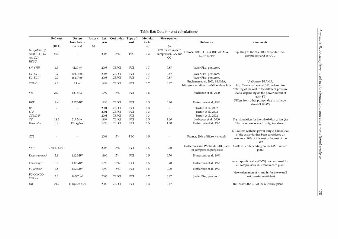
Appendix B. Assumptions used in the simulations and the conventional analyses
170
Table B.6: Data for cost calculationse
Ref. cost Design
characteristic
Factor x Ref.
year
Cost index Type of
cost
Modular
factor
Size exponent
Reference
Comments
(106 €) (varies) (‐) (‐) (‐)
GT system, ref.
plant (GT1, C1
and CC)
50.0 ‐ 2006 15% PEC 1.3
0.90 for expander/
compressor, 0.67 for
CC
Framer, 2006; SGT4‐4000F, 286 MW,
Tout,fg= 1071°F
Splitting of the cost: 40% expander, 35%
compressor and 25% CC
HRSG
SH, SHII 1.3 4120 m2 2005 CEPCI FCI 1.7 0.87 Javier Pisa, pers.com.
EV, EVII 3.7 20474 m2 2005 CEPCI FCI 1.7 0.87 Javier Pisa, pers.com.
EC, ECII 2.0 16247 m2 2005 CEPCI FCI 1.7 0.87 Javier Pisa, pers.com.
COND 9.0 1 kW 1999 CEPCI FCI 1.7 0.87 Buchanan et al., 2000, BEAMA,
http://www.taftan.com/xl/condens.htm
Uo (Source: BEAMA,
http://www.taftan.com/xl/condens.htm
STs 26.0 120 MW 1999 15% FCI 1.5 ‐ Buchanan et al., 2000
Splitting of the cost to the different pressure
levels, depending on the power output of
each ST
HPP 1.4 3.37 MW 1990 CEPCI FCI 1.3 0.80 Tsatsaronis et al., 1991 Differs from other pumps, due to its larger
size (> 300 kW)
IPP ‐ ‐ 2001 CEPCI FCI 1.3 ‐ Turton et al., 2002
LPP ‐ ‐ 2001 CEPCI FCI 1.3 ‐ Turton et al., 2002
COND P ‐ ‐ 2001 CEPCI FCI 1.3 ‐ Turton et al., 2002
CT 18.3 217 MW 1999 CEPCI FCI 1.5 1.00 Buchanan et al., 2000 Ebs. simulation for the calculation of the QCT
De‐aerator 0.9 190 kg/sec 1990 CEPCI FCI 1.5 1.00 Tsatsaronis et al., 1991 The mass flow refers to outgoing stream
GT2 ‐ ‐ 2006 15% PEC 1.5 ‐ Framer, 2006 ; different models
GT system with net power output half as that
of the expander has been considered as
reference. 40% of this cost is the cost of the
GT2
ST4a Cost of LPST 2008 15% FCI 1.5 0.90 Tsatsaronis and Winhold, 1984 (used
for comparison purposes)
Costs differ depending on the LPST in each
plant
Recycle compr.b 3.8 1.42 MW 1990 15% FCI 1.5 0.70 Tsatsaronis et al., 1991
CO2 compr. c 3.8 1.42 MW 1990 15% FCI 1.5 0.70 Tsatsaronis et al., 1991 mean specific value (€/kW) has been used for
all compressors, different in each plant
FG compr. d 3.8 1.42 MW 1990 15% FCI 1.5 0.70 Tsatsaronis et al., 1991
FG COND&
COOLs 2.0 16247 m2 2005 CEPCI FCI 1.7 0.87 Javier Pisa, pers.com.
New calculation of hc and hn for the overall
heat transfer coefficient
DB 21.9 14 kg/sec fuel 2008 CEPCI FCI 1.3 0.67 Ref. cost is the CC of the reference plant
Appen
dix B. Assumption
s used in
the simulation
s and the con
ventional an
alyses 170

Appendix B. Assumptions used in the simulations and the conventional analyses
171
MCM
0.2
1 MWth fuel
2001 CEPCI FCI 3.0 ‐ Möller et al., 2006
No exponent used, due to the already
realized extrapolation of the given cost
MCM HTHX 2.0 16,247 m2 5 2005 CEPCI FCI 1.7 0.87 Javier Pisa, pers.com. New calculation of hc and hn for the overall
heat transfer coefficient
MCM LTHX 2.0 16,247 m2 5 2005 CEPCI FCI 1.7 0.87 Javier Pisa, pers.com. New calculation of hc and hn for the overall
heat transfer coefficient
NGPH 2.0 16,247 m2 2 2005 CEPCI FCI 1.7 0.87 Javier Pisa, pers.com. New calculation of hc and hn for the overall
heat transfer coefficient
Air PH 2.0 16,247 m2 5 2005 CEPCI FCI 1.7 0.87 Javier Pisa, pers.com. New calculation of hc and hn for the overall
heat transfer coefficient
CLC 16.2 180 m3 2000 CEPCI PEC 1.2 0.60 Klara (2007), Wolf et al. (2005),
Lyngfeld and Thunman (2005)
CAU 50%> FCItot of
to ref. plant ‐ ‐ FCI 3.0
sensitivity analysis
0.60 Abu‐Zahra et al., 2007, IPCC 2005
Splitting of the cost: 55% absorber, 18%
stripper and 27% remaining components
a ST4 and ST5 are considered part of the IPST in the MEA plant
b Recycle compr (C6, AZEPs) c CO2 compr.(C2‐C5, AZEPs, CLC; C3‐C6, MEA) d FG compr (C2, MEA) e 1€ = 1$
Appen
dix B. Assumption
s used in
the simulation
s and the con
ventional an
alyses 171

Appendix B. Assumptions used in the simulations and the conventional analyses
172
Table B.7: Assumptions involved in the economic analysis (reference year: 2009)
Parameter (units) Value
Average general inflation rate (%) 3
Average nominal escalation rate (%) 3
Average nominal escalation rate for NG (%) 4
Beginning of design and construction period 2011
Date of commercial operation 2013
Plant economic life (years) 20
Plant life for tax purposes (years) 15
Plant financing fractions and required returns on capital
Type of financing Common equity Debt
Financing fraction (%) 50 50
Required annual return (%) 12 8
Resulting average cost of money (%) 10
Average combined income tax rate (%) 30
Average property tax rate (% of PFI)
Average insurance rate (% of PFI)
Average capacity factor (%) 85
Labor positions for opening and maintenance 30
Average labor rate (€/h) 50
Annual fixed operating and maintenance costs (106 €) 1.5
Annual fixed operating and maintenance costs
at full capacity (103 €) 624
Unit cost of fuel (€/GJ‐LHV:50,015 MJ/kg) 7
Allocation of plant facilities investment to the
individual years of design and construction (%)
Jan. 1‐Dec. 31, 2011 40
Jan. 1‐Dec. 31, 2012 60
Rao, 2002. The height of the regenerator agrees with that of the absorber, while its diameter is
calculated based on its volume.
Generalized cost equations for common components of the plants, as an example for
similar‐sided equipment are provided in Appendix D.
After the estimation of the FCI of the plant, a detailed economic analysis following the
TRR method (see Appendix A) was realized for each plant. The main assumptions made for
this analysis are shown in Table B.7.
B.2.3 Application of the exergoeconomic analysis
The exergoeconomic analysis consists of a group of linear equations stated at the component
level. The sum of all costs entering a component (cost of incoming streams plus investment
cost of the component) must be equal to the cost of the streams exiting the component. The
cost of air and water provided to the plants is considered to be zero.
Dissipative components (e.g., throttling valves, coolers, condensers, gas cleaning units)
serve productive components in a system, facilitating an overall effective operation, cost
reduction or achievement of required emission standards. Thus, costs associated with
purchasing and operating a dissipative component are usually charged either to the

Appendix B. Assumptions used in the simulations and the conventional analyses
173
component(s) served by it or to the final product(s) of the system (Lazzaretto and Tsatsaronis,
2006). In this thesis, the costs related to dissipative equipment are charged to the components
served by it (e.g., the cost of each cooler is charged to the subsequent compressor served).
When more than one component is served by a dissipative component, the cost is
apportioned to all of the components served, using weighting factors.
For example, the investment cost of a CT is charged to the condensers/coolers supplied
with cooling water, using the respective heat transfer rates (Q ) as weighting factors. The
condenser serves the components of the steam cycle, allowing the perpetuation of the
water/steam cycle. The cost of the condenser is, therefore, shared by the components
constituting the steam cycle, depending on the contribution of each component to their total
exergy destruction. For the condenser and CT (Figure B.3), the exergy costing equation (with
specific cost of water equal to zero) is written as:
c c
COND CT COND CT COND CTC Z Z C c E Z Z c E c E E Z Z1 2
1 2 1 1 1 2 1 1 2 0 1
Figure B.3: Connection between condenser and cooling tower
However, because COND CTc E E Z Z1 1 2 0 , an imaginary value, diffC , is introduced to
maintain the cost balance:
COND CT diffc E E Z Z C1 1 2 0
To calculate the diffC and the exergy destruction used as weighting factor for the cost sharing,
the exergoeconomic analysis must be realized. When all dissipative components have been
accounted for, they are removed from the cycle and the analysis is repeated.
B.2.4 Application of the LCA
In an LCA, the component variables, the consumption and the release of materials are
identified and quantified (Fiaschi and Lombardi, 2002). In order to identify the material inlet
flows, the overall life cycle of each component of the plant must be considered and, hence, the
1 The auxiliary equation of the condenser is c1=c2.
COND CT
1
2
3
4

Appendix B. Assumptions used in the simulations and the conventional analyses
174
phases of construction, operation and dismantling must be taken into account. For the
quantification of the materials needed, it is necessary to approximate the size of the plant and
collect information about the main materials, their production processes and weights, as well
as the scrap output of all equipment assembled for the plant. To shift from the manufactured
materials to the raw substances and emissions inventory, the commercially available software
Package SimaPro 7.1 has been used (SimaPro, 2006).
The selection of construction materials, based on strength, corrosion resistance and cost
of fabrication, is vital to process design estimates. Expertise about equipment can also assist
in the final selection of materials. In general, carbon steel is used whenever possible because
of its low cost and ease of fabrication (Seider, 2004). Details about component design and
suitable construction materials are obtained from equipment design handbooks and
manufacturing leaflets. Typical construction materials for conventional process equipment
are listed in Table B.8.
Table B.8: Typical construction materials for process equipment
Component Materials
GT expandera Discs: High‐strength steels, Vanes: Cobalt‐ Nickel‐based alloys, Blades: Ni‐based
alloys
Compressora Discs: High‐strength low steel, Blades: low‐carbon steel
CCa Cans: Ni‐based sheet superalloys
ST Valve chest, shafts, discs: Alloy steel, Steam rings, cylinders: Carbon steel, Blades:
Stainless steel
HRSG Carbon/Stainless steel
Storage/Process vessel Steel/Reinforced steel
Condenser Copper‐ Ni‐alloys, Stainless steel, Titanium, Brass
De‐aerator Carbon/Stainless steel
Pump Carbon/Stainless steel, Cast iron, Nickel, Titanium
CTb Steel, Stainless steel, PVC, FRP, Concrete, Polyethylene
a The materials used in GT systems are in the range of metallurgical alloys from high‐strength steel to
lightweight aluminum or titanium and are mainly temperature‐resistant. b Materials to enhance corrosion resistance, reduce maintenance, and promote reliability and long service life
are used
As mentioned in section 3.2.3, in order to quantitatively assess environmental impacts, the
environmental impact indicator Eco‐indicator 99 is used. The Eco‐indicator 99 impact
assessment method (“Hierarchist‐Average“ database version) (SimaPro, 2006) is used in a
similar way as costs in the exergoeconomic analysis. Standard Eco‐indicator 99 points
summarize the environmental impacts associated with the complete upstream chain
(production and distribution) of 1 kg of each required raw material. Design estimates depend
on the required construction materials. In order to accomplish this it is necessary to:
a) Estimate the equipment weight using product information sheets and mechanical
design characteristics provided by manufacturers. In most cases, weight estimation is a
function of the operating conditions and the mechanical design requirements of each
unit. Thus, the equipment weight could be estimated based merely on mechanical design
calculations and on “rules of thumb”. Reference values are extrapolated taking the
operating conditions of the considered processes into consideration.

Appendix B. Assumptions used in the simulations and the conventional analyses
175
b) Estimate the percentage of each construction material required to manufacture a
component. This estimate is based on available manufacturing information data sheets
and mechanical design standards.
For the estimation of environmental impacts, the environmental boundaries of the
systems have been defined to incorporate all relevant processes (see section B.2.5). The
construction stage includes the consumption of construction materials for the manufacture of
system components, while the operating stage includes the consumption of fossil fuel as
inflow stream and the gas emissions (mainly CO2 and NOx) as outflow streams.
The design characteristics, the construction materials, the references used and the
environmental impact of the chosen materials, represented by the ECO‐indicator, are
presented for all types of components in Table B.9.

Appendix B. Assumptions used in the simulations and the conventional analyses
176
Table B.9: Design data for plant components
Component, k Design Parameter Design characteristics Used construction
materials
Eco‐indicator
99
(Pts/t)
Material
composition
(%,w/w)
References
GT1/GT2 Power Conventional turbine for 200‐300 MW power output Steel 86 25 Nuovo Pignone, 2009;
Exhaust volume flowrate Steel high alloy 910 75 Soares, 2002.
C1
Steel 86 33.33
C2‐C5 (C3‐C6 for Discharge pressure Centrifugal Steel low alloy 110 44.45
Cooper, 2009.
MEA plant) Volume flowrate
Cast iron 240 22.22
CC/ DB Fuel/air mass flowrate Sequential combustion with air Steel 86 33.34 Nuovo Pignone, 2009;
Steel high alloy 910 66.66 Seider et al., 2004.
STs Power 30‐60 MW power output Steel 86 25 Mitsubishi, 2009;
Exhaust volume flowrate Steel high alloy 910 75 Soares, 2002.
MCM reactor Thermal power Rhodium enriched
(catalyzator) 12.000.000 1.24
MCM/
HT<HX Membrane density
Mixed conducting membrane with oxygen ion
vacancies
Zinc coating (catalyst
support) per m2 49 11.16
Eriksson et al., 2007; Griffin et al., 2005;
Sundkvist, 2005, 2007; Reinke, 2005;
Kolbitsch, 2008; Seider et al., 2004.
Thermal power Monolit (membrane) volume = 47.18 m3 Steel high alloy 910 56.94
Surface to volume ratio = >500 m2/m3 Cast iron 240 30.66
CLC reactors
(AR & FR) Oxygen carrier capacity Energy density = 15 MW/m3 Steel high alloy 910 65 www.hyundai.eu;
Oxygen production rate = 37 mol O2/(m3.s) Cast iron 240 35 Linderholm, 2008, Wolf, 2005; Kolbitsch,
2009; www.durofelguera.com;
Catalyzator active area = 0.26 m2/g Naqvi, 2007; Naqvi, 2006.
Two interconnected pressurised fluidised bed reactors
with a cyclone system
Solids inventory = 100‐ 200 kg/MW
Solids residence time:
AR = 4.8 s, FR = 60 s
Gas velocity:
AR = 10 m/s, FR = 15 m/s
Oxygen carrier particles (NiO):
mean diameter = 150 μm
average density = 2400 kg/m3
Appen
dix B. Assumption
s used in
the simulation
s and the con
ventional an
alyses 176

Appendix B. Assumptions used in the simulations and the conventional analyses
177
HXs / HRSG Heat transfer area SH/RH, Air HX, NGPH
Heat transfer coefficient OD=2 in, ID=1.738 Steel 86 26 Ganapathy, 1991, Perry and Green, 1997;
tube length=10 ft, thickn.=0.120 in Steel high alloy 910 74 committees.api.org/standards, 2009; Seider
et al., 2004
fin density=2 fin/in, height=0.500 in
fin thickn.=0.075 in
COND/ COOL/ EV/
EC tube OD=2 in, ID=1.770 in Steel 86 100 Soares, 2002; Seider et al., 2004.
tube length=10 ft, thickn.=0.105 in
fin density=4 fin/in, height=0.750 in
fin thickn.=0.050 in
CT Water volume flowrate Hyperbolic counterflow Natural‐draft tower with
PVC film fill Concrete 3.8 91 www.gammonindia.com, June 2009;
Heat transfer area PVC (high impact) 280 9 www.evaptech.com, June 2009; Gould et al.,
1999 ;
http://process-equipment.globalspec.com;
www.alpine‐bau.de, June 2009.
Storage/Process
Vessel Perry and Green, 1997.
De‐aerator Volume flowrate capacity Deaerating boiler feedwater Steel 86 100 Gestra, 2009;
Pressure committees.api.org/standards, 2009.
PUMP (P) Fluid volume flowrate (GPM) Centrifugal Steel 86 35 www.pumpexpert.com, May 2009;
Discharge pressure Cast iron 240 65 Bloch et al., 1998; www.chempump.com,
2009.
CAU
Absorber: packed vessel. Height
and diameter
Stripper: regeneration heat
requirement
Steel
Steel high alloy
86
910
1%
99%
Rubin and Rao, 2002; Rennie, 2006;
www.sulzerchemtech.com
Appen
dix B. Assumption
s used in
the simulation
s and the con
ventional an
alyses 177

Appendix B. Assumptions used in the simulations and the conventional analyses
178
B.2.5 Application of the exergoenvironmental analysis
The operating parameters of this analysis are the same as those considered in the economic
analysis: 20 years of operation with 7446 h/yr. To determine the impact associated with the
production of electricity, the same group of equations as in the exergoeconomic analysis is
used. The difference here is that the cost rates are replaced with environmental impacts. The
environmental impacts associated with the production of methane and with each component
separately are correlated in the system of linear equations.
The environmental impact associated with the production of electricity in each energy
conversion system is compared, taking the environmental impact of the outflow streams,
such as CO2 and NOx emissions, into consideration (Table B.10). In the case of the three oxy‐
fuel technologies, AZEP 85, AZEP 100 and CLC, the environmental impact associated with
the CO2 sequestration of the separated CO2 stream is also considered, using LCA data
reported in recent publications (Khoo et al, 2006). The part of the pollutant formation related
to the amount of CO2 captured in each plant is subtracted from the overall environmental
impact.
Exergoenvironmental variables are calculated in order to identify the relative importance
of each component with respect to their environmental impact and, to identify the magnitude
and location of the environmental impact caused by system inefficiencies. The results are
used to evaluate and compare the environmental performance of the four considered power
plants.
Table B.10: EI of incoming and exiting streams of the systems (Eco‐indicator 99, HA)
Product System boundaries Eco‐indicator
(Pts/t)
Reference
Natural gas Production and distribution 180.0
CO2 Emission 5.4
Goedkoop and Spriensma, 2000
SimaPro, 2006
CO2 Sequestration 4.9 Khoo et al., 2006
CH4 Emission 114.6
NOx Emission 2749.4
Goedkoop and Spriensma, 2000
SimaPro, 2006

Appendix C. Design estimates for heat exchangers
179
Appendix C
Design estimates for construction,
operational costs and environmental
impacts of heat exchangers
C.1 Calculation of the surface area, A
To calculate the area A of a HX in m2, Equation C.1 is used:
logo
QA
U
(C.1)
Here, Q is the heat transfer rate (W), ΔTlog is the logarithmic mean temperature difference,
log
ln
A B
A
B
, with ΔTA and ΔTB the temperature differences on sides A and B (K),
respectively, and Uo is the overall heat transfer coefficient (reciprocal of the overall thermal
resistance) that differs depending on the design and operation, as well as the working fluid of
the HX considered (W/m2K).
C.1.1 Calculation of the overall heat transfer coefficient
The overall heat transfer coefficient is a function of several variables such as tube size,
spacing, and gas velocity (Ganapathy, 2003). For HRSGs in combined cycle power plants
operating with natural gas, the overall heat transfer coefficient of a HX is calculated as
(Ganapathy, 1991):
lno o o oi o
o o i i m i i
d d d dff ff
U h h d K d d
1 1
24 (C.2)
Here, ih is the tube‐side coefficient, oh is the gas‐side coefficient, od and id are the outside
and inside diameters of a tube, respectively, off and iff are the fouling factors on the outside
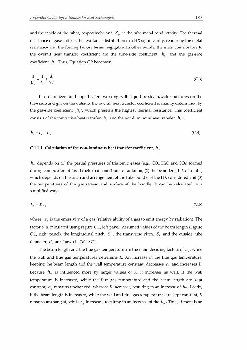
Appendix C. Design estimates for heat exchangers
180
and the inside of the tubes, respectively, and mK is the tube metal conductivity. The thermal
resistance of gases affects the resistance distribution in a HX significantly, rendering the metal
resistance and the fouling factors terms negligible. In other words, the main contributors to
the overall heat transfer coefficient are the tube‐side coefficient, ih , and the gas‐side
coefficient, oh . Thus, Equation C.2 becomes:
o
o o i i
d
U h h d
1 1 (C.3)
In economizers and superheaters working with liquid or steam/water mixtures on the
tube side and gas on the outside, the overall heat transfer coefficient is mainly determined by
the gas‐side coefficient ( oh ), which presents the highest thermal resistance. This coefficient
consists of the convective heat transfer, ch , and the non‐luminous heat transfer, Nh :
o c Nh h h (C.4)
C.1.1.1 Calculation of the non‐luminous heat transfer coefficient, Nh
Nh depends on (1) the partial pressures of triatomic gases (e.g., CO2, H2O and SO2) formed
during combustion of fossil fuels that contribute to radiation, (2) the beam length L of a tube,
which depends on the pitch and arrangement of the tube bundle of the HX considered and (3)
the temperatures of the gas stream and surface of the bundle. It can be calculated in a
simplified way:
N gh K (C.5)
where g is the emissivity of a gas (relative ability of a gas to emit energy by radiation). The
factor K is calculated using Figure C.1, left panel. Assumed values of the beam length (Figure
C.1, right panel), the longitudinal pitch, LS , the transverse pitch, TS and the outside tube
diameter, od are shown in Table C.1.
The beam length and the flue gas temperature are the main deciding factors of g , while
the wall and flue gas temperatures determine K. An increase in the flue gas temperature,
keeping the beam length and the wall temperature constant, decreases g and increases K.
Because Nh is influenced more by larger values of K, it increases as well. If the wall
temperature is increased, while the flue gas temperature and the beam length are kept
constant, g remains unchanged, whereas K increases, resulting in an increase of Nh . Lastly,
if the beam length is increased, while the wall and flue gas temperatures are kept constant, K
remains unchanged, while g increases, resulting in an increase of the Nh . Thus, if there is an

Appendix C. Design estimates for heat exchangers
181
increase in the flue gas or wall temperature and/or in the beam length, Nh will increase as
well.
Figures C.2‐C.4 were obtained using data derived from Figure C1. Figure C.2 shows the
variation of g with the flue gas temperature and the beam length, while Figure C.3 shows
the variation of K with the wall and flue gas temperatures. Figure C.4 combines the two
previous figures, showing the overall influence of Nh by the wall and flue gas temperatures
and the beam length. Next to each figure the polynomial trendlines of the different curves are
shown. It can be seen that Nh is not strongly influenced by the wall temperature, especially
for higher flue gas temperatures and smaller beam lengths. Thus, one general equation has
been assumed for each different beam length (trendlines of Figure C.4).
Figure C.1: Graphs used for the estimation of the hN (left panel) and beam length evaluation (right
panel). (Source: Ganapathy, 1991)
Table C.1: Beam length L
L od
TS *
LS *
(m) (in) (in) (in)
5 1.25 2.50 2.80
6 1.50 3.00 3.36
7 2.00 4.00 4.48
9 2.50 5.00 5.60
( T oS d 2 and .L TS S 1 12 )
Fuel Excess air % 1 Bituminous coals 20 2 Natural gas 10 3 No.2 oil 10 4 No. 6 oil 10 5 Blast furnace gas 10 6 Blast furnace gas 30 7 No. 2 oil 20
S L

Appendix C. Design estimates for heat exchangers
182
0.06
0.08
0.10
0.12
0.14
0.16
0.18
600 800 1000 1200 1400 1600 1800 2000
Temperature (°F)
L=5 L=6 L=7
0
10
20
30
40
50
600 800 1000 1200 1400 1600 1800 2000
Temperature (°F)
K
W all Temperature 400°F Wall Temperature 600°F
W all Temperature 500°F Wall Temperature 700°F
0.0
0.5
1.0
1.5
2.0
2.5
3.0
3.5
4.0
4.5
0 200 400 600 800 1000 1200 1400 1600 1800 2000
Temperature (°F)
hN, T=800, L=6 hN, T=700, L=6 hN, T=600, L=6hN, T=800, L=7 hN, T=700, L=7 hN, T=600, L=7hN, T=800, L=5 hN, T=700, L=5 hN, T=600, L=5hN, T=800, L=9 hN, T=700, L=9 hN, T=600, L=9
Polynomial trendlines
Figure C.2: Estimation of gas emissivity at different flue gas temperatures and beam lengths (L), g
Polynomial trendlines
Figure C.3: Estimation of the factor K at different wall and flue gas temperatures
Polynomial trendlines
Figure C.4: Estimation of the hN at different temperatures and beam lengths
L=5: ‐2E‐08x2 + 2E‐05x + 0.1096
L=6: ‐2E‐08x2 + 2E‐05x + 0.1196
L=7: ‐2E‐08x2 + 2E‐05x + 0.1246
L=9: ‐2E‐08x2 + 2E‐05x + 0.1546
T=400: 1E‐05x2 ‐ 0.0071x + 7.4156
T=500: 1E‐05x2 ‐ 0.0076x + 8.3206
T=600: 1E‐05x2 ‐ 0.0082x + 9.2255
T=700: 1E‐05x2 ‐ 0.0092x + 10.930
L=5: E‐07x2 + 0.0002x + 0.8674
L=6: E‐07x2 + 0.0001x + 0.9767
L=7: 5E‐07x2 + 9E‐05x + 1.0314
L=9: 8E‐07x2 ‐ 0.0002x + 1.3593
Btu/ft hFNh 2
g

Appendix C. Design estimates for heat exchangers
183
( . . )( . / )( )
( )
w g
c w
c w
p TK p p
p p L
0 8 1 6 1 0 38 1000 (C.6)
cp and wp are the partial pressures of CO2 and water vapor included in the gas stream, and
gT is the average gas temperature (K). Nh is approximated anew using Equation C.5 and the
new trendlines, obtained for streams with dominant concentrations of H2O or CO2 (shown in
Table C.2).
Table C.2: Approximation of the hN with mass ratios 8:1 H2O and 25:1 CO2 (based on the respective
element content in the conventional flue gases)
Beam length (m) hN
8:1 H2O 25:1 CO2
L=5 1E‐06x2 + 0.0012x + 3.1418 6E‐07x2 + 0.0006x + 1.7772
L=6 1E‐06x2 + 0.0011x + 3.2511 7E‐07x2 + 0.0005x + 1.8865
L=7 1E‐06x2 + 0.001x + 3.3058 8E‐07x2 + 0.0005x + 1.9411
L=9 1E‐06x2 + 0.001x + 3.3604 8E‐07x2 + 0.0004x + 1.9958
C.1.1.2 Calculation of the convective heat transfer coefficient, ch
The convective heat transfer coefficient is calculated using Equation C.7:
co
kh Nu
d
12 (C.7)
Nu is the Nusselt number ( . .. Re PrNu 0 6 0 330 033 ) and k the thermal conductivity in Btu/fthF.
To calculate the Nusselt number, Re (Reynolds number) and Pr (Prandtl number) are
estimated as:
Re oGd
12 (C.8)
Pr pC
k
(C.9)
G is the gas velocity in lb/ft2h, μ the viscosity in lb/fth and pC the specific heat in Btu/lbF. The
gas mass velocity G is defined as:
g
w t o
WG
N S d L
12 (C.10)
Here, Nw is the number of tubes wide and Wg the gas flow in lb/h.

Appendix C. Design estimates for heat exchangers
184
Due to lack of input data, assumptions include steady flue gas and mass velocity of 35 ft/sec
(10m/sec) and 5000 lb/ft2h, respectively, throughout the HRSG. With these values, the gas
density, g , is found to be 0.04 lb/ft3
gg
G
V3600; an intermediate value of g is calculated
with data derived from EbsilonProfessional. However, the viscosity, the specific heat and the
conductivity vary with temperature (Table C.3) and result in different Re and Nu numbers.
Also, the diameter of the tubes, od , depends on the HX. ch has been estimated for different
temperatures using a constant od of 2 in. (Figure C.5). When od is different than 2 in., the
coefficient has been adjusted using the equation:
'c
o o
Nu kh
d d
12 (C.11)
Here, 'od is a diameter different than 2 in.
Table C.3: Gas and steam properties (Source: Ganapathy, 1991)
Air (dry) GT exhaust gas
Temperature
(°F)
Cp
(Btu/LbF)
μ
(Lb/fth)
k
(Btu/fthF)
Temperature
(°F)
Cp
(Btu/LbF)
μ
(Lb/fth)
k
(Btu/fthF)
200 0.2439 0.0537 0.0188 200 0.2529 0.0517 0.0182
400 0.2485 0.0632 0.0221 400 0.2584 0.0612 0.0218
800 0.2587 0.0809 0.0287 600 0.2643 0.0702 0.0253
1200 0.2696 0.0968 0.0350 800 0.2705 0.0789 0.0287
1600 0.2800 0.1109 0.0412 1000 0.2767 0.0870 0.0321
2000 0.2887 0.1232 0.0473
Water vapor CO2
Temperature
(°F)
Cp
(Btu/LbF)
μ
(Lb/fth)
k
(Btu/fthF)
Temperature
(°F)
Cp
(Btu/LbF)
μ
(Lb/fth)
k
(Btu/fthF)
200 0.4532 0.0315 0.0134 200 0.2162 0.0438 0.0125
400 0.4663 0.0411 0.0197 400 0.2369 0.0544 0.0177
600 0.4812 0.0506 0.0261 600 0.2543 0.0645 0.0227
800 0.4975 0.0597 0.0326 800 0.2688 0.0749 0.0274
1000 0.5147 0.0687 0.0393 1000 0.2807 0.0829 0.0319
1200 0.5325 0.0773 0.0462 1200 0.2903 0.0913 0.0360
1400 0.5506 0.0858 0.0532 1400 0.2980 0.0991 0.0400
1600 0.5684 0.0939 0.0604 1600 0.3041 0.1064 0.0435
1800 0.5857 0.1019 0.0678 1800 0.3090 0.1130 0.0468
2000 0.6019 0.1095 0.0753 2000 0.3129 0.1191 0.0500
Air, GT exhaust gases and CO2 streams present similar behavior, with respect to
temperature changes. The ch of steam streams, on the other hand, presents a much more
intense change with temperature.
The composition of the gas passing through the secondary HRSGs differs from the
conventional GT flue gases and, therefore, ch must be adjusted properly. To reflect the
percentage of CO2 and H2O included in a stream, the curves representing pure CO2 and H2O
steams, shown in Figure C.5, are shifted depending on the relative concentrations of the two
elements. In other words, the molecular fractions of carbon dioxide and water vapor in a
stream are used as weighting factors for recalculating the multipliers of the CO2 and H2O
curves (e.g., Table C.4).

Appendix C. Design estimates for heat exchangers
185
5
10
15
20
25
30
35
0 500 1000 1500 2000 2500
Temperature, FGT exhaust gas dry Air CO2
Linear trendlines
Figure C.5: Estimation of the hc of different gases at different temperatures
Table C.4: Estimation of the hc for high concentrations of CO2 and H2O
hc
2:1 CO2:H2O 32:1 CO2:H2O
0.0069x + 9.214 0.0054x + 8.420
C.1.1.3 Calculation of the tube‐side coefficient, ih
5.00
7.00
9.00
11.00
13.00
15.00
17.00
19.00
21.00
23.00
25.00
0 200 400 600 800 1000 1200
ho/hi (Btu/ft²Fh)
ho hi
Figure C.6: Influence of the ho and hi variation on the Uo
ih only influences the total heat transfer coefficient when it is small (Figure C.6). When gas
flows on the outer side of tubes and high heat transfer coefficients are calculated for the tube
side, the overall coefficient is governed by the gas‐side resistance. Assuming the other
H2O: 0.0100x + 10.904
CO2: 0.0053x + 8.3433
GT: 0.0042x + 10.036
Air: 0.0034x + 10.322
Btu/ft hFch 2
Btu/ft hFoU 2
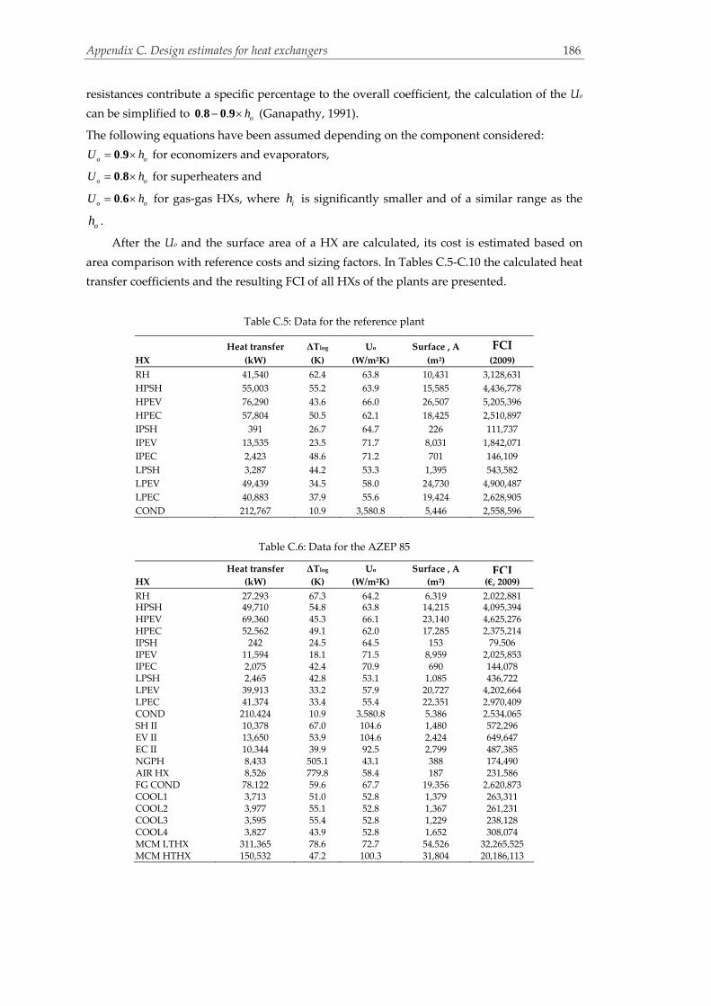
Appendix C. Design estimates for heat exchangers
186
resistances contribute a specific percentage to the overall coefficient, the calculation of the Uo
can be simplified to . . oh 0 8 0 9 (Ganapathy, 1991).
The following equations have been assumed depending on the component considered:
.o oU h 0 9 for economizers and evaporators,
.o oU h 0 8 for superheaters and
.o oU h 0 6 for gas‐gas HXs, where ih is significantly smaller and of a similar range as the
oh .
After the Uo and the surface area of a HX are calculated, its cost is estimated based on
area comparison with reference costs and sizing factors. In Tables C.5‐C.10 the calculated heat
transfer coefficients and the resulting FCI of all HXs of the plants are presented.
Table C.5: Data for the reference plant
Heat transfer ΔTlog Uo Surface , A FCI HX (kW) (K) (W/m²Κ) (m²) (2009)
RH 41,540 62.4 63.8 10,431 3,128,631
HPSH 55,003 55.2 63.9 15,585 4,436,778
HPEV 76,290 43.6 66.0 26,507 5,205,396
HPEC 57,804 50.5 62.1 18,425 2,510,897
IPSH 391 26.7 64.7 226 111,737
IPEV 13,535 23.5 71.7 8,031 1,842,071
IPEC 2,423 48.6 71.2 701 146,109
LPSH 3,287 44.2 53.3 1,395 543,582
LPEV 49,439 34.5 58.0 24,730 4,900,487
LPEC 40,883 37.9 55.6 19,424 2,628,905
COND 212,767 10.9 3,580.8 5,446 2,558,596
Table C.6: Data for the AZEP 85
Heat transfer ΔTlog Uo Surface , A FCIHX (kW) (K) (W/m²Κ) (m²) (€, 2009)
RH 27,293 67.3 64.2 6,319 2,022,881 HPSH 49,710 54.8 63.8 14,215 4,095,394 HPEV 69,360 45.3 66.1 23,140 4,625,276 HPEC 52,562 49.1 62.0 17,285 2,375,214 IPSH 242 24.5 64.5 153 79,506 IPEV 11,594 18.1 71.5 8,959 2,025,853 IPEC 2,075 42.4 70.9 690 144,078 LPSH 2,465 42.8 53.1 1,085 436,722 LPEV 39,913 33.2 57.9 20,727 4,202,664 LPEC 41,374 33.4 55.4 22,351 2,970,409 COND 210,424 10.9 3,580.8 5,386 2,534,065 SH II 10,378 67.0 104.6 1,480 572,296 EV II 13,650 53.9 104.6 2,424 649,647 EC II 10,344 39.9 92.5 2,799 487,385 NGPH 8,433 505.1 43.1 388 174,490 AIR HX 8,526 779.8 58.4 187 231,586 FG COND 78,122 59.6 67.7 19,356 2,620,873 COOL1 3,713 51.0 52.8 1,379 263,311 COOL2 3,977 55.1 52.8 1,367 261,231 COOL3 3,595 55.4 52.8 1,229 238,128 COOL4 3,827 43.9 52.8 1,652 308,074 MCM LTHX 311,365 78.6 72.7 54,526 32,265,525 MCM HTHX 150,532 47.2 100.3 31,804 20,186,113

Appendix C. Design estimates for heat exchangers
187
Table C.7: Data for the AZEP 100
Heat transfer ΔTlog Uo Surface , A FCI HX (kW) (K) (W/m²Κ) (m²) (€, 2009)
RH 21,331 69.0 61.8 4,998 1,649,469
HPSH 30,867 45.3 61.5 11,063 3,292,736
HPEV 58,306 37.2 65.5 23,945 4,764,861
HPEC 44,177 56.0 62.5 12,633 1,808,108
IPSH 1,660 33.6 65.4 755 318,432
IPEV 29,009 25.6 72.0 15,747 3,309,015
IPEC 5,198 41.2 70.8 1,781 328,922
LPSH 2,551 41.6 53.0 1,158 462,291
LPEV 43,941 32.2 57.9 23,568 4,699,592
LPEC 43,235 36.1 55.5 21,573 2,880,176
COND 213,104 10.9 3,580.8 5,455 2,562,119
SH II 13,187 68.6 105.4 1,823 686,095
EV II 16,680 55.2 104.8 2,883 755,487
EC II 12,639 38.5 92.3 3,560 600,791
NGPH 8,433 511.9 43 382 172,468.5
AIR HX 10,121 779.4 58.5 222 268,813
FG COND 91,439 58.6 67.5 23,121 3,059,209
COOL1 4,358 50.9 52.8 1,622 303,140
COOL2 4,669 55.0 52.8 1,607 300,736
COOL3 4,224 55.4 52.8 1,445 274,204
COOL4 4,496 43.8 52.8 1,943 354,779
MCM LTHX 366,209 79.3 72.7 63,529 36,853,012
MCM HTHX 177,096 47.9 100.3 36,859 22,950,277
Table C.8: Data of the plant with CLC
Heat transfer ΔTlog Uo Surface , A FCI HX (kW) (K) (W/m²Κ) (m²) (€, 2009)
RH 26,688 73.5 62.4 5,815 1,881,804
HPSH 36,418 46.5 62.0 12,621 3,692,758
HPEV 63,015 38.8 65.6 24,753 4,904,542
HPEC 47,749 54.7 62.4 14,000 1,977,257
IPSH 1,328 32.0 65.3 635 274,129
IPEV 26,268 24.3 71.9 15,057 3,182,549
IPEC 4,707 41.4 70.9 1,604 300,168
LPSH 2,635 41.8 53.0 1,190 473,220
LPEV 44,688 32.4 57.9 23,825 4,744,024
LPEC 39,692 38.1 55.6 18,724 2,546,260
COND 197,313 10.9 3,580.8 5,051 2,396,131
SH II 819 32.7 91.2 274 132,036
EV II 3,686 29.1 99.8 1,270 370,248
EC II 2,794 73.3 97.0 393 88,229
NGPH 10,582 269.6 44 889 359,222.7
FG COND 101,416 80.6 71.1 17,716 2,426,575
COOL1 4,242 50.4 52.4 1,607 300,747
COOL2 4,542 54.4 52.4 1,592 298,249
COOL3 4,062 54.5 52.4 1,424 270,650
COOL4 4,292 42.8 52.4 1,914 350,132

Appendix C. Design estimates for heat exchangers
188
Table C.9: Data for MEA‐0
Heat transfer ΔTlog Uo Surface , A FCI HX (kW) (K) (W/m²Κ) (m²) (€, 2009)
RH 41,540 63.7 64.0 10,185 3,064,369
HPSH 55,519 54.2 63.8 16,049 4,551,454
HPEV 76,481 43.8 66.0 26,435 5,193,210
HPEC 57,949 50.3 62.1 18,545 2,525,057
IPSH 363 26.4 64.6 213 105,794
IPEV 13,036 23.3 71.7 7,817 1,799,282
IPEC 2,334 48.6 71.2 675 141,318
LPSH 3,299 44.3 53.3 1,400 545,022
LPEV 49,229 34.5 58.0 24,610 4,879,876
LPEC 41,165 37.0 55.6 20,003 2,696,976
COND 51,017 13.6 3,580.8 1,051 738,649
COOL CAU 47,121 61.6 65.0 11,778 1,701,151
COOL1 4,179 69.4 52.7 1,141 223,285
COOL2 3,941 62.6 52.7 1,193 232,104
COOL3 3,565 63.0 52.7 1,074 211,703
COOL4 3,796 53.2 52.7 1,354 259,001
Table C.10: Data for MEA‐0.2
Heat transfer ΔTlog Uo Surface , A FCI HX (kW) (K) (W/m²Κ) (m²) (€, 2009)
RH 41,540 63.8 64.0 10,185 3,170,644
HPSH 55,519 63.5 63.5 16,147 4,734,122
HPEV 76,481 66.0 66.0 26,435 5,373,316
HPEC 57,949 62.1 62.1 18,545 2,612,628
IPSH 363 64.3 64.3 214 110,040
IPEV 13,036 71.7 71.7 7,817 1,861,683
IPEC 2,334 71.2 71.2 675 146,219
LPSH 3,299 52.9 52.9 1,408 566,895
LPEV 49,229 58.0 58.0 24,610 5,049,115
LPEC 41,165 55.6 55.6 20,003 2,790,510
COND 120,636 3,580.8 3580.8 2,485 1,615,906
COOL CAU 47,121 765.1 65.0 11,778 1,760,149
COOL1 7,333 76.7 52.7 1,455 285,325
COOL2 3,941 62.9 52.7 1,193 240,154
COOL3 3,565 56.6 52.7 1,074 219,045
COOL4 3,796 71.4 52.7 1,354 267,984
C.1.2 Design of the tubes
The number and design of tubes in HXs are specified by setting their outside diameter and
wall thickness. Smaller diameter tubes yield higher heat transfer coefficients, but larger
diameter tubes are easier to clean and more rugged. Here, all outside diameters of the HXs
are assumed to be 2.5 in, with the exception of the condenser, the IPHRSG and the secondary
HRSG, where they are assumed to be 2 in, because of the smaller water/steam mass flows.
Fins can increase heat transfer and decrease the surface area of a HX. Four fins per in. of
0.75 in. height are assumed for economizers, condensers and coolers, and two fins per in. of
0.50 in. height are chosen for superheaters, reheaters and gas‐gas HXs. To account for using
fins in the HXs, Figure C.7 has been used. Assuming 16.5 MMBtuh are transferred without
including fins and that 17.5 or 16.6 MMBtuh are transferred using four or two fins per in. of

Appendix C. Design estimates for heat exchangers
189
0.75/0.50 in. height, respectively, the Uo values are increased by 6% or 0.6% (17.5/16.5=1.06
and 16.6/16.5=1.006). This increase has been considered here and it is included in the
presented results.
The area of each finned tube is calculated as:
o
o o
dnA d h h bd bh nb24 4 2 4 1
24 12 (C.12)
Here, n is the fin density, h is the fin height and b is the fin thickness.
Figure C.7: Effect of fin geometry on performance. (Source: Ganapathy, 1991)
C.1.3 Materials
Materials widely used for the construction of tubes in HXs are those of group 178 of the
grades A, C and D that stand for carbon steel, group 213 of the grades T11, T22, T5 and T91
that stand for intermediate alloys and group 213 of grades Tp‐304, Tp‐316, Tp‐321 and Tp‐347
that represent the use of stainless steel. The letters H and L indicate high and low carbon,
respectively. Series 300 includes 0.15% carbon, a minimum of 16% chromium and sufficient
nickel or manganese. The materials of the HXs comprising the HRSGs have been chosen
depending on the outer wall temperature. For all of the plants, the materials have been kept
the same for similar components, since the size and operating conditions are comparable. The
maximum allowed temperatures for the most commonly used materials are shown in Table
C.11:

Appendix C. Design estimates for heat exchangers
190
Table C.11: Main construction materials of HRSGs (Ganapathy, 1991)
Material Maximum allowance Component
temperature, °C
SA‐178, grade A 482 HPEV, HPEC, IPEV,
IPEC
SA‐178, grade C 510 ‐
SA‐213, grade T2 552 ‐
SA‐213, grade T11 566 ‐
SA‐213, grade T22 607 ‐
SA‐213, grade T91 649 RH, HPSH
SA‐213, grade Tp 304 H, 321 H 760 ‐ The names of the metals follow the American Society of Mechanical Engineers (ASME) specifications.
The appropriate materials for the rest of the HXs have been chosen in a similar way. In Table
C.12 the design estimates related to the reference plant that lead to the calculation of the
weight of the HXs are presented as an example of the calculations performed for all of the
plants.

Appendix C. Design estimates for heat exchangers
191
Table C.12: Design estimates for the HXs of the reference plant
od id tube
lenght
tube
thickn.
fin
density
fin
height
fin
thickn.
mat.
densityafinned tube
area
number of
tubes
casing
width
tubes/
row
weight/
tube
weight
of fins
weight
of tubes
weight
of casing
total
weight
Heat Exchanger (in) (in) (ft) (in) (fin/in) (in) (in) (lb/in) (ft2) (n) (in) (n) (lb) (lb) (t) (t) (t)
HPSH 2.5 2.380 10 0.120 2 0.500 0.075 0.289 22.65 7,408 563.5 86 31.9 26.0 195 62.4 257
HPEV 2.5 2.395 10 0.105 4 0.750 0.050 0.283 58.38 4,887 458.4 70 27.4 54.1 181 40.5 221
HPEC 2.5 2.395 10 0.105 4 0.750 0.050 0.283 58.38 3,397 382.9 58 27.4 54.1 126 28.2 154
RH 2.5 2.380 10 0.120 2 0.500 0.075 0.289 22.65 4,958 461.7 70 31.9 26.0 130 41.9 172
IPSH 2.0 1.880 10 0.120 2 0.500 0.075 0.289 18.72 130 72.5 11 24.8 21.7 3 1.0 4
IPEV 2.0 1.895 10 0.105 4 0.750 0.050 0.283 49.22 1,756 255.5 42 21.8 45.8 54 12.6 66
IPEC 2.0 1.895 10 0.105 4 0.750 0.050 0.283 49.22 153 78.3 12 21.8 45.8 5 1.2 6
LPSH 2.5 2.380 10 0.120 2 0.500 0.075 0.289 22.65 663 171.4 26 31.2 26.0 17 5.8 23
LPEV 2.5 2.395 10 0.105 4 0.750 0.050 0.283 58.38 4,560 442.9 68 27.4 54.1 169 37.8 206
LPEC 2.5 2.395 10 0.105 4 0.750 0.050 0.283 58.38 3,581 393.0 60 27.4 54.1 132 29.7 162
COND 2.0 1.895 10 0.105 4 0.750 0.050 0.283 49.22 5,797 460.8 76 21.8 45.8 37 40.9 77
a Material densities of 0.289 and 0.283 lb/in are associated with stainless and carbon steel, respectively
Appen
dix C. Design
estimates for heat exchan
gers 191

Appendix C. Design estimates for heat exchangers
192

Appendix D
Generalized costing equations
The following equations are based on cost calculations realized for this thesis and are shown
here as a generalized guide for fixed capital cost calculations of similar‐sized components.
The sources used are shown in Table B.6 of Appendix B.
1. Gas turbine system1,2 (reference year: 2009; for other GT systems, see “Gas Turbine World”;
Framer, 2006).
0.9
6_ 65.6 10
290net
GT system
WCost
Expander
exp _ 0.4 ander GT systemCost Cost
Compressor
_ 0.35 compressor GT systemCost Cost
Combustion chamber
_ 0.25 compressor GT systemCost Cost
Or
0.67
621.9 10628.5
fg
CC
mCost
1 Pressure ratio: 16.8 2 The total cost has been shared among the three main components of the system as following: 40% to the expander,
35% to the compressor and 25% to the CC.

Appendix D. Generalized costing equations
194
2. Heat recovery steam generator
Reheater, Superheater
0.87
6// 3
1.3 10468.24.1 10
SH RH CEPSI
SH RH
A CICost
Evaporator
0.87
63
3.7 10468.220.5 10
EV CEPSI
EV
A CICost
Economizer
0.87
63
2 10468.216.3 10
EC CEPSI
EC
A CICost
3. Condenser
0.87
61.9 10213.0 390.6
COND CEPSI
COND
Q CICost
4. ST system (reference year 2009)3
0.9
6_ 26.4 10
120
ST sys
WCost
_
_
_
1.5
2
1.5 2
HPST ST systemtot
IPST ST systemtot
LPST ST systemtot
tot HPST IPST LPST
HPST
WCost Cost
W
IPST
WCost Cost
W
LPST
WCost Cost
W
Where,
W W W W
3 High pressure: 124 bar

Appendix D. Generalized costing equations
195
5. Pumps4
a) For 0.3 MWPW
o Oulet Pressure ~ 5 bar
22.9 2,328 61,233357.6
CEPSIPump P P
CICost W W
o Oulet Pressure ~ 25 bar
24.05 3, 277 86, 205357.6
CEPSIPump P P
CICost W W
o Oulet Pressure ~ 100 bar
24.3 3,795 102,268357.6
CEPSIPump P P
CICost W W
o Oulet Pressure ~ 130 bar
24.8 4,197 113,100357.6
CEPSIPump P P
CICost W W
For 0.3 MWPW
0.8
61.4 103.4 357.6
CEPSIP
Pump
CIWCost
6. Cooling Tower
61.8 10216.9 390.6
CEPSICT
CIQCost
7. De‐aerator
34.9 10357.6
CEPSIDeaerator s w
CICost m m
II. Added components in plants with CO2 capture
1. Steam Turbine (reference year 2009)
0.9
ST LPST
LPST
WCost Cost
W
4 Centrifugal; carbon steel pumps, including the cost of motors (Turton et al., 2002)
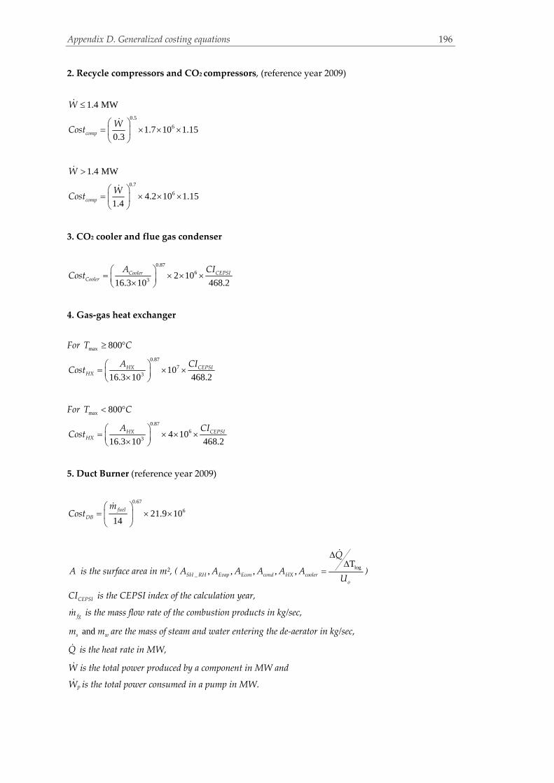
Appendix D. Generalized costing equations
196
2. Recycle compressors and CO2 compressors, (reference year 2009)
1.4 MWW
0.5
61.7 10 1.150.3
comp
WCost
1.4 MWW
0.7
64.2 10 1.151.4comp
WCost
3. CO2 cooler and flue gas condenser
0.87
63
2 10468.216.3 10
Cooler CEPSI
Cooler
A CICost
4. Gas‐gas heat exchanger
For max 800 T C
0.87
73
10468.216.3 10
CEPSIHX
HX
CIACost
For max 800 T C
0.87
63
4 10468.216.3 10
CEPSIHX
HX
CIACost
5. Duct Burner (reference year 2009)
0.67
621.9 1014
fuel
DB
mCost
A is the surface area in m², (log
_
T, , , , ,
SH RH Evap Econ cond HX cooler
o
Q
A A A A A AU
)
CEPSICI is the CEPSI index of the calculation year,
fgm is the mass flow rate of the combustion products in kg/sec,
and s wm m are the mass of steam and water entering the de‐aerator in kg/sec,
Q is the heat rate in MW,
W is the total power produced by a component in MW and
PW is the total power consumed in a pump in MW.
References
Abad, A., Mattisson, T., Lyngfelt, A. and Rydén, M. (2006) Chemical‐looping combustion in a 300
W continuously operating reactor system using a manganese‐based oxygen carrier, Fuel, 85,
1174‐1185.
Abad, A., Mattisson, T., Lyngfelt, A. and Johansson, M. (2007) The use of iron oxide as oxygen
carrier in a chemical‐looping reactor, Fuel, 86, 1021‐1035.
Abu‐Zahra, M.R.M., Niederer, J.P.M, Feron, P.H.M., Versteeg, G.F. (2007) CO2 capture from
power plants Part II. A parametric study of the economical performance based on mono‐
ethanolamine, International Journal of Greenhouse Gas Control, I, 135‐142.
Afgan, N., et al. (1996) New Developments in Heat Exchangers, ISBN: 905699512X.
Anderson, R., MacAdam, S., Viteri, F., Davies, D., Downs, J. and Paliszewski, A. (2008) Adapting
Gas Turbines to Zero Emission Oxy‐fuel Power Plants, Proceedings of the ASME Turbo Expo,
Berlin, G2008‐51377.
Anderson, K. and Johnsson, F. (2006) Process evaluation of an 865 MWe lignite fired O2/CO2
power plant, Energy Conversion and Management, 47 (18‐19), 3487‐3498.
Anderson, K., Johnsson, F. and Strömberg, L. (2003) Large Scale CO2 Capture‐Applying the
Concept of O2/CO2 Combustion to Commercial Process Data, VGB PowerTech 83, Heft 10, 29–33.
Aspen Plus, Aspentech, http://www.aspentech.com, accessed: December, 2009.
Bejan, A., Tsatsaronis, G. and Moran, M. (1996) Thermal Design and Optimization, J. Wiley, New
York.
Benedict, M. and Gyftopoulos, E. P. (1980) Economic Selection of the Components of an Air
Separation Process, in: Thermodynamics: Second Law Analysis (R.A. Gaggioli, Ed.) A.C. S.
Symposium Series, 122, 195‐203.
Benson, S. M. and Orr, Jr., F. M. (2008) Carbon Dioxide Capture and Storage, MRS Bulletin, 33,
303‐305.
Bergmann, E. and Schmidt, K. R. (1965) Zur kostenwirtschaftlichen Optimierung der
Warmeaustauscher für die regenerative Speisewasservorwarmung im Dampfkraftwerk ‐ ein
Storungsverfahren mit der Exergie, in: Energie und Exergie, VDI‐Verlag, Düsseldorf, 63‐89.
Beyer, J. (1979) Einige Probleme der praktischen Anwendung der exergetischen Methode in
wärmewirtschaftlichen Untersuchungen industrieller Produktionsprozesse II,
Energieanwendung 28 (2), 66‐70.
Beyer, J. (1978) Einige Probleme der praktischen Anwendung der exergetischen Methode in
wärmewirtschaftlichen Untersuchungen industrieller Produktionsprozesse I, Energieanwendung,
27 (6), 204‐208.

References
198
Beyer, J. (1972) Zur Aufteilung der Primärenergiekosten in Koppelprozessen auf Grundlage der
Strukturanalyse, Energieanwendung, 21 (6), 179‐183.
Bloch, H. P. and Soares, C. (1998) Process Plant Machinery, Second Edition, Butterworth‐
Heinemann, USA, 249‐276.
Bolhàr‐Nordenkampf, J., Pröll, T., Kolbitsch, P., Hofbauer, H. (2008) Performance of a NiO‐based
oxygen carrier for Chemical Looping Combustion and reforming in a 120kW unit, 9th
International Conference on Greenhouse Gas Technologies, Washington DC.
Bolland, O. and Mathieu, P. (1998) Comparison of two CO2 removal options in combined cycle
power plants, Energy Conversion and Management, 39, 1653‐1663.
Bolland, O. (1991) Comparative evaluation of advanced combined cycle alternatives, Journal of
Engineering for Gas Turbines and Power, 113, 190‐197.
Bottino, A., Comite, A., Capannelli, G., di Felice, R. and Pinacci, P. (2006) Steam reforming of
methane in equilibrium membrane reactors for integration in power cycles, Catalysis Today, 118,
214–222.
Boyano, A., Tsatsaronis, G., Morosuk, T. and Marigota, A. M. (2010) Advanced
exergoenvironmental analysis of a steam methane reforming system for hydrogen production,
ASME, IMECE2010‐38551.
Boyano, A., Tsatsaronis, G., Morosuk, T. and Blanco‐Marigorta, A. M. (2009) Advanced exergetic
analyses of chemical processes, Proceedings of the ASME 2009 International Mechanical
Engineering Congress and Exposition, Lake Buena Vista, IMECE2009‐10463.
Brandvoll, Ø. and Bolland, O. (2004) Inherent CO2 Capture Using Chemical Looping Combustion
in a Natural Gas Fired Power Cycle, ASME Journal of Engineering for Gas Turbines and Power,
126, 316‐321, GT‐2002‐30129.
Brandvoll, Ø., Kolbeinsen, L., Olsen, N. and Bolland, O. (2003) Chemical Looping Combustion –
Reduction of nickel oxide/nickel aluminate with hydrogen, in: Proceedings of the Sixth Italian
Conference on Chemical and Process Engineering, Pisa, Italy, Chemical Engineering
Transactions, 3, 105‐110.
Climate Change 2007: Synthesis Report (2007) (Pachauri, R. K. and Reisinger, A., Eds.), IPCC,
Geneva, 104.
Chen, L., Hong, Q., Lin, J. and Dautzenberg, F. (2007) Hydrogen production by coupled catalytic
partial oxidation and steam methane reforming at elevated pressure and temperature, Journal of
Power Sources, 164, 803–808.
Cooper Turbocompressor Inc., Centrifugal Compressors,
http://www.fluidenergy.com/pdf/cooper_ta_msg.pdf, accessed: May, 2009.
Cziesla, F., Tsatsaronis, G. and Gao, Z. (2006) Avoidable Thermodynamic Inefficiencies and Costs
in an Externally‐Fired Combined‐Cycle Power Plant, Energy ‐ The International Journal, 31, 1472‐
1489.
EES, Engineering Equation Solver, http://www.mhhe.com/engcs/mech/ees, accessed: July, 2009.
Eisermann, W., Hasberg, W. and Tsatsaronis, G. (1984) THESIS – Ein Rechnerprogramm zur
Simulation und Entwicklung von Energieumwandlungsanlagen, Brennstoff Wärme Kraft, 36
(1/2), 45‐51.
References
199
Eisermann, W. (1979) Analysis of Processes for Production of Synthetic Gaseous Fuels, Final
Report, NATO Fellowship Contract No. 430‐402‐566‐8, University of Kentucky.
El Sayed, Y. M. (2003) The Thermoeconomics of Energy Conversions, Pergamon, 1st edition.
El‐Sayed, Y. M. and Tribus, M. (1983) Strategic use of thermoeconomics for system improvement,
in: Efficiency and Costing Second Law Analysis of Processes, A. C. S. Symposium Series, 235, 215‐
238.
El‐Sayed, Y. M. and Aplenc, A. J. (1970) Application of the thermoeconomic approach to the
analysis and optimization of a vapor‐compression desalting system, Trans. ASME, J. Eng. Power,
92, 17‐26.
El‐Sayed Y. M. and Evans, R. B. (1970) Thermoeconomics and the design of heat systems, Trans.
ASME, J. Eng. Power, 92, 27‐34.
Environmental management, Life cycle assessment, Principles and framework (2006), ISO
14040:2006.
Environmental Technology Best Practice Programme (ETBPP), Life Cycle Assessment ‐ An
Introduction for Industry, ET257 GUIDE, http://www.tangram.co.uk, accessed: March, 2000.
Buchanan, T., DeLallo, M., Schoff, R., White, J., Wolk, R. (2000) Evaluation of Innovative Fossil
Fuel Power Plants with CO2 Removal, Palo Alto, CA, U. S. Department of Energy — Office of
Fossil Energy, Germantown, MD and U. S. Department of Energy/NETL, Pittsburgh, PA: 2000.
1000316.
Eriksson, O., Finnveden, G., Ekvall, T. and Bjöklund, A. (2007) Life cycle assessment of fuels for
district heating: A comparison of waste incineration, biomass‐and natural gas combustion,
Energy policy, 35 (2), 1346‐1362.
Evans, R. B., Kadaba, P. V. and Hendrix, W. A. (1983) Essergetic functional analysis for process
design and synthesis, in: Efficiency and Costing Second Law Analysis of Processes, A. C. S.
Symposium Series, 235, 239‐261.
Evans, R. B. and Tribus, M. (1965) Thermo‐Economics of Saline Water Conversion, Industrial and
Engineering Chemistry, Process Design and Development, 4 (2), 195‐206.
Evans, R.B. and Tribus, M. (1962) A Contribution to the Theory of Thermoeconomics, UCLA,
Dept. of Engr.: Report No. 62/63, Los Angeles, CA.
Fehring, T. H. and Gaggioli, R. A. (1977) Economics of feedwater heater replacement, Trans.
ASME, J. Eng. Power, 99, 482‐489.
Fiaschi, D. and Lombardi, L. (2002) Integrated Gasifier Combined Cycle Power Plant with
Integrated CO2‐H2S removal: Performance Analysis, Life Cycle Assessment and Exergetic Life
Cycle Assessment, International Journal of Applied Thermodynamics, 5 (1), 13‐24.
Framer, R. (2006) Gas Turbine World 2006 Handbook, Pequot Publishing, Fairfield, CT.
Frangopoulos, C. A. (1994) CGAM problem: Definition and conventional solution, Energy ‐ The
International Journal, 19 (3), 323‐342.
Frangopoulos, C. A. (1992) Optimal synthesis and operation of thermal systems by the
thermoeconomic functional approach, J Eng Gas Turbines Power, 114, 707‐714.

References
200
Frangopoulos, C. A. (1988) Functional decomposition for optimal design of complex thermal
systems, Energy ‐ The International Journal, 13 (3), 239–244.
Frangopoulos, C. A. (1987) Thermo‐economic functional analysis and optimization, Energy ‐ The
International Journal, 12 (7), 563–71.
Frangopoulos, C. A. (1983) Thermoeconomic functional analysis: a method for optimal design or
improvement of complex thermal systems, Dissertation, Georgia Institute of Technology.
Gaggioli, R. A., El‐Sayed, Y .M., El‐Nashar, A. M. and Kamaluddin, B. (1986) Second Law
Efficiency and Costing Analysis of a Combined Power and Desalination Plant, in: Computer‐
Aided Engineering of Energy Systems (Gaggioli, R. A., Ed.), 2‐3, ASME, New York, 77‐85.
Gaggioli, R. A. (1983) Second Law Analysis for Process and Energy Engineering, in: Efficiency
and Costing Second Law Analysis of Processes (Gaggioli, R. A., Ed.), A. C. S. Symposium Series,
235, 3‐50.
Gaggioli, R. A. (1977) Proper evaluation and pricing of energy, Proc. Int. Conf. Energy Use
Management, 11 (24‐28), 31‐43.
Gaggioli, R. A., Rodriguez, L. and Wepfer, W. J. (1978) A Thermodynamic‐Economic Analysis of
the Synthane Process, Final Report prepared for the Pittsburgh Energy Technology Center, U.S.
D.O.E., Contract No. EY‐77‐S‐02‐4589‐1.
Ganapathy, V., (2003) Industrial Boilers and Heat Recovery Steam Generators, Marcel Dekker,
New York.
Ganapathy, V., (1991) Waste Heat Boiler Desktop, The Fairmont Press, Lilburn, GA.
GE Enter Software LLC (2000), GateCycle, Menlo Park, CA.
Gestra, A. G., Deaerating Plant for Boiler Feedwater C4. FLOWSERVE ‐ Flow Control Division,
http://www.flowserve.com/files/Files/Literature/ProductLiterature/FlowControl/Gestra/813938.p
df, accessed: May, 2009.
Goedkoop, M., Spriensma, R. (2000) The Eco‐indicator 99: A Damage Oriented Method for Life
Cycle Impact Assessment, Methodology Report, Amersfoort, Netherlands.
Griffin, T., Sundkvist, S. G., Asen, K. and Bruun, T. (2005) Advanced Zero Emissions Gas Turbine
Power Plant, Journal of Engineering for Gas Turbines and Power, 127, 81‐85.
Grubbström, J. (2008) Chemical Looping Combustion, Status of Development, ALSTOM,
Chemical Looping Programme, Elforsk.
Guthrie, K. (1974) Process plant estimating, evaluation and control, ISBN: 0‐910460‐5‐1.
Herzog, H. (2001) What Future for Carbon Capture and Sequestration?, Environmental Science
and Technology, 35, 148.
Hesselmann, K. (1986) Heat exchanger networks – An exergoeconomical evaluation, in:
Computer‐Aided Engineering of Energy Systems, ASME, W.A.M., New York, 2‐3, 23‐34.
Horn, R., Williams, K., Degenstein, N., Bitsch‐Larsen, A., Nogare, D. D., Tupy, S. and Schmidt, L.
(2007) Methane catalytic partial oxidation on autothermal Rh and Pt foam catalysts: Oxidation
and reforming zones, transport effects, and approach to thermodynamic equilibrium, Journal of
Catalysis, 249, 380–393.

References
201
Hossain, M. M., de Lasa, H. I. (2008) Chemical‐looping combustion (CLC) for inherent CO2
separation – a review. Chemical Engineering Science, 63, 4433‐4451.
INSPIRE, RTN supported by the European Communityʹs Sixth Framework Programme,
http://www.http.www.mc‐inspire.net, accessed: July, 2009.
IPCC, Special Report on Carbon Dioxide Capture and Storage, Prepared by Working Group III of
the Intergovernmental Panel on Climate Change (2005) (Metz, B., Davidson, O., de Coninck, H.
C., Loos, M. and Meyer, L. A. Eds.), Cambridge University Press, Cambridge, United Kingdom
and New York, NY, USA.
Ishida, M. and Jin, H. (1994) A novel combustor based on chemical‐looping reactions and its
reaction kinetics, Journal of Chemical Engineering of Japan, 27, 296‐301.
Jericha, H., Lukasser, A. and Gatterbauer, W. (2000) Der Graz Cycle für Industriekraftwerke
gefeuert mit Brenngasen aus Kohle‐ und Schwerölvergasung, VDI Berichte 1566, VDI Conference
Essen, Germany.
Jericha, H. and Fesharaki, M. (1995) The Graz Cycle 1500 C Max Temperature‐CO2 Capture with
CH4‐O2 Firing, ASME paper 95‐CTP‐79, ASME Cogen‐Turbo Power Conference, Vienna.
Jericha, H. (1985) Efficient Steam Cycles with Internal Combustion of Hydrogen and
Stoichiometric Oxygen for Turbines and Piston Engines, CIMAC Conference Paper, Oslo,
Norway.
Jin, H. and Ishida, M. (2004) A new type of coal gas fueled chemical‐looping combustion, Fuel, 83,
2411‐2417.
Johannessen, E. and Jordal, K. (2005) Study of a H2 separating membrane reactor for methane
steam reforming at conditions relevant for power processes with CO2 capture. Energy Conversion
and Management, 46, 1059–1071.
Johansson, M., Mattisson, T., Lyngfelt, A. (2006) Comparison of oxygen carriers for Chemical‐
Looping Combustion, Thermal Science, 10, 93‐107.
Jordal, K., Bredesen, R., Kvamsdal, H. and Bolland, O. (2004) Integration of H2‐separating
membrane technology in gas turbine processes for CO2 capture, Energy, 29, 1269–1278.
Kakaras, E., Doukelis, A., Giannakopoulos, D. and Koumanakos, A. (2005) Emission reduction
technologies for the fossil fuel fuelled electricity generation sector, Scientific conference HELECO.
Katalytisch, R. M. (2005) Stabilisierte Verbrennung von Ch4/Luft Gemischen und H2O‐ und CO2‐
Verdünnten Ch4/Luft Gemischen über Platin unter Hochdruckbedingungen. Dissertation.
Eidgenössischen Technischen Hochschule Zürich, 26, 11‐17.
Keenan, J. H. (1932) A steam chart for second law analysis, Trans. ASME, 54 (3), 195–204.
Kelly, S., Tsatsaronis G. and Morosuk, T. (2009) Advanced Exergetic Analysis: Approaches for
Splitting the Exergy Destruction into Endogenous and Exogenous Parts, Energy – The
International Journal, 34 (3), 384‐391.
Kelly, S. (2008) Energy systems improvement based on endogenous and exogenous exergy
destruction, Dissertation, Technische Universität Berlin, Berlin, Germany.
Kenney, W. F. (1984) Energy conservation in the process industries, Academic Press, Inc.

References
202
Khoo, H. H. and Tan, R. B. H. (2006) Life Cycle Evaluation of CO2 Recovery and Mineral
Sequestration Alternatives, Environmental Progress, 25 (3), 208‐217.
Klara, J. M. (2007) Chemical‐Looping Process in a Coal‐to‐Liquids, Independent Assessment of
the potential of the OSU Chemical Looping Concept, U.S. Department of Energy, National
Energy Technology Laboratory, DOE/NETL‐2008/1307.
Knoche, K. F. and Funk, J. E. (1977) Entropie‐Produktion, Wirkungsgrad und Wirtschaftlichkeit
der thermodynamischen Erzeugung syntetischer Brennstoffe, Der Schwefelsäure‐Hybrid‐Prozess
zur thermochemischen Wasserspaltung, BWK 29 (1), 23‐27.
Knoche, K. F. and Hesselmann, K. (1986) Exergoeconomical Analysis of chemical processes –
Evaluation of an Air separation plant, in: Computer‐Aided Engineering of Energy Systems,
ASME, W.A.M., New York, 2‐3, 35‐43.
Knoche, K. F. and Hesselmann, K. (1985) Exergoökonomische Bewertung einer Luftzerlegungs‐
Anlage, Chem.‐Ing.‐Techn., 57, 602‐609.
Knoche, K. F., Richter, H. (1968) Verbesserung der Reversibilität von Verbrennungs‐Prozessen,
Brennstoff‐Wärme‐ Kraft, 5, 205‐210.
Kolbitsch, P., Pröll, T., Hofbauer H. (2008) Modeling of a 120kW chemical looping combustion
reactor system using a NiO oxygen carrier, Chemical Engineering Science, 64, 99‐108.
Kotas, T. J. (1985) The exergy method of thermal plant analysis, Butterworths, London.
Kothandaraman, A., Nord, L., Bolland, O., Herzog, H. J. and McRae, G. J. (2009) Comparison of
solvents for post‐combustion capture of CO2 by chemical absorption, Energy Procedia, 1, 1373‐
1380.
Kvamsdal, H., Jordan, K. and Bolland, O. (2007) A quantitative comparison of gas turbine cycles
with CO2 capture, Energy, 32 (1), 10‐24.
Lazzaretto, A. and Andreatta, R. (1995) Algebraic formulation of a process‐based exergy‐costing
method, in: Symposium on thermodynamics and the design, analysis, and improvement of
energy systems (Krane R. J., Ed.), 35. ASME, New York, 395–403.
Lazzaretto, A. and Tsatsaronis, G. (2006) SPECO: A Systematic and General Methodology for
Calculating Efficiencies and Costs in Thermal Systems, Energy ‐ The International Journal, 31,
1257‐1289.
Lazzaretto, A. and Tsatsaronis, G. (1997) On the Quest for Objective Equations in Exergy Costing,
Proceedings of the ASME, Advanced Energy Systems Division (Ramalingam, M. L., Lage, J. L.,
Mei, V. C., and Chapman, J. N., Eds.), 37, 197‐210.
Lewis, W. K. and Gilliland, E.R. (1954) Production of pure carbon dioxide, US patent No. 2665972.
Lin, L. and Tsatsaronis, G. (1993) Cost Optimization of an Advanced IGCC Power Plant Concept
Design, Thermodynamics and the Design, Analysis, and Improvement of Energy Systems – 1993
(Richter, H. J., Ed.), 30 (266), 157‐166.
Linderholm C., Abad A., Mattisson T. and Lyngfelt A. (2008) 160 h of chemical‐looping
combustion in a 10 kW reactor system with a NiO‐based oxygen carrier, The 4th Trondheim
Conference on CO2 Capture, Transport and Storage International Journal of Greenhouse Gas
Control, 2 (4), 520‐530.

References
203
Ludwig, E. (2001) Applied Process Design III, 3rd Edition, ISBN: 0‐8841‐5651‐6.
Lyngfelt, A., Leckner, B. and Mattisson, T. (2001) A fluidized‐bed combustion process with
inherent CO2 separation; application of chemical‐looping combustion, Chemical Engineering
Science, 56, 3101‐3113.
Lyngfelt, A. and Thunman, H. (2005) Construction and 100 h of operational experience of a 10‐
kW chemical looping combustor, in: The CO2 Capture and Storage Project (CCP) for Carbon
Dioxide Storage in Deep Geologic Formations For Climate Change Mitigation, 1, 625‐646.
Matlab 7, The MathWorks, Matlab online Documentation,
http://www.mathworks.com/access/helpdesk/help/techdoc/math/f1‐85462.html, accessed:
December, 2009.
Mattison, T. and Lyngfelt, A. (2001) Applications of chemical‐looping combustion with capture of
CO2, 2nd Nordic minisymposium on CO2 capture and storage, Göteborg, Sweden.
Meyer, L., Tsatsaronis, G., Bushgeister, J. and Schebek, L. (2009) Exergoenvironmental analysis
for evaluation of the environmental impact of energy conversion systems, Energy ‐ The
International Journal 34, 75‐89.
MITSUBISHI Heavy Industries, LTD, Steam Turbine Generator, Standard Turbine Frames,
http://www.mhi.co.jp/en/products/ pdf/at_turbine.pdf, accessed: April, 2009.
Moeller, B., Torisson, T., Assadi, M., Sundkvist, S. G. and Asen, K. I. (2006) AZEP Gas Turbine
Combined Cycle Power Plants ‐ Thermo‐economic Analysis, International Journal of
Thermodynamics, 9, 21‐28.
Moran, M. J. (1982) Availability Analysis – A Guide to efficient energy use, Prentice‐Hall, Inc..
Morosuk, T. and Tsatsaronis, G. (2009a) Advanced Exergy Analysis for Chemically Reacting
Systems – Application to a Simple Open Gas‐Turbine System, International Journal of
Thermodynamics, 12 (3), 105‐111.
Morosuk, T. and Tsatsaronis, G. (2009b) Advanced Exergetic Evaluation of Refrigeration
Machines Using Different Working Fluids, Energy ‐ The International Journal, 34 (12), 2248‐2258.
Morosuk, T., and Tsatsaronis, G. (2008a) A New Approach to the Exergy Analysis of Absorption
Refrigeration Machines Energy ‐ The International Journal, 33 (6), 890‐907.
Morosuk, T. and Tsatsaronis, G. (2008b) How to Calculate the Parts of Exergy Destruction in an
Advanced Exergetic Analysis, in: Proceedings of the 21st International Conference on Efficiency,
Costs, Optimization, Simulation and Environmental Impact of Energy Systems (Ziebik, A.,
Kolenda, Z. and Stanek, W. Eds.), Cracow‐Gliwice, 185‐194.
Morosuk, T. and Tsatsaronis, G. (2007) Exergoeconomic Evaluation of Refrigeration Machines
Based on Avoidable Endogenous and Exogenous Costs, in: Proceedings of the 20th International
Conference on Efficiency, Cost, Optimization, Simulation and Environmental Impact of Energy
Systems (Mirandola, A., Arnas, O. and Lazzaretto, A., Eds.), Padova, 1, 1459‐1467.
Morosuk, T. and Tsatsaronis, G. (2006a) Splitting the exergy destruction into endogenous and
exogenous parts – application to refrigeration machines, in: Proceedings of the 19th International
conference on efficiency, cost, optimization, simulation and environmental impact of energy
systems (Frangopoulos, C., Rakopoulos, C. and Tsatsaronis, G., Eds.), Aghia Pelagia: Crete, 1,
165–172.

References
204
Morosuk, T. and Tsatsaronis, G. (2006b) The ‘Cycle Method’ used in the exergy analysis of
refrigeration machines: from education to research, in: Proceedings of the 19th International
conference on efficiency, cost, optimization, simulation and environmental impact of energy
systems (Frangopoulos, C., Rakopoulos, C. and Tsatsaronis, G., Eds.), Aghia Pelagia: Crete, 1,
157‐163.
Obert, E. F. and Gaggioli, R. A. (1963) Thermodynamics, McGraw‐Hill, New York.
Naqvi, R. (2006) Analysis of Natural Gas‐Fired Power Cycles with Chemical Looping
Combustion for CO2 Capture, Dissertation, Norwegian University of Science and Technology.
Naqvi, R. and Bolland, O. (2007) Multi‐stage chemical looping combustion (CLC) for combined
cycles with CO2 capture. Int. J. of Greenhouse Gas Control, 1, 19‐30.
Naqvi, R., Bolland, O. and Wolf, J. (2005) Off‐Design Evaluation of a natural gas fired Chemical
Looping Combustion combined cycle with CO2 capture, Proceedings of The 18th International
Conference on Efficiency, Cost, Optimization, Simulation and Environmental Impact of Energy
Systems (ECOS), Trondheim, Norway, 827‐834.
Nuovo Pignone S.p.A. GE Oil & Gas ‐ Gas Turbines,
http://www.geoilandgas.com/businesses/ge_oilandgas/en/downloads/gas_turb_cat.pdf, accessed:
April, 2009.
Perry R. H. and Green, D. W. (1997) Perry´s Chemical Engineers´ Handbook, Seventh Edition,
McGraw‐Hill Companies, Inc., New York.
Peters, M. S. (2003) Plant design and economics for chemical engineers, 5th Edition, New York,
ISBN: 0‐07‐239266‐5.
Petrakopoulou F., Boyano A., Cabrera M. and Tsatsaronis G. (2010a) Exergoeconomic and
exergoenvironmental analyses of a combined cycle power plant with chemical looping
technology, International Journal of Greenhouse Gas Control, In press, DOI:
10.1016/j.ijggc.2010.06.008.
Petrakopoulou F., Tsatsaronis G., Boyano A. and Morosuk T. (2010b) Exergoeconomic and
Exergoenvironmental Evaluation of power plants including CO2 capture, Carbon Capture &
Storage Special Issue of Chemical Engineering Research and Design, In press, DOI:
10.1016/j.cherd.2010.08.001.
Petrakopoulou F., Tsatsaronis G. and Morosuk T. (2010c) Conventional Exergetic and
Exergoeconomic analyses of a power plant with chemical looping combustion for CO2 capture,
International Journal of Thermodynamics, Vol. 13 (3), pp. 77‐86.
Petrakopoulou F., Boyano A., Cabrera M. and Tsatsaronis G. (2010d) Exergy‐based analyses of an
advanced zero emission plant, International Journal of Low‐Carbon Technologies, Vol. 5 (4), pp.
231‐238.
Petrakopoulou F., Tsatsaronis G., Morosuk T. and Carassai A. (2010e) Conventional and
advanced Exergetic Analyses applied to a combined cycle power plant, ECOS 2010, Lausanne,
Switzerland, pp. 1363‐1371.
Petrakopoulou F., Tsatsaronis G., Morosuk T. and Carassai A. (2010f) Advanced Exergoeconomic
Analysis applied to a complex energy conversion system, ASME IMECE 2010, Vancouver,
Canada, CD‐ROM, IMECE2010‐38555.

References
205
Reistad, G. M. (1970) Availability: Concepts and Applications, Dissertation, The University of
Wisconsin‐Madison, USA.
Rennie, (2006) Corrosion and materials selection for amine service, Materials forum, 30, (Wuhrer,
R. and Cortie, M., Eds.), Inst of Materials Engineering Austrialasia, Ltd.
Richter, H. J. and Knoche, K. F. (1983) Reversibility of combustion processes, ACS Symposium
Series, 235, 9971‐9985.
Rubin, E. S. and Rao, A. B. (2002) A Technical, Economic and Environmental Assessment of
Amine‐based CO2 Capture Technology for Power Plant Greenhouse Gas Control, U.S.
Department of Energy, National Energy Technology Laboratory, DOE/DE‐FC26‐00NT40935.
Sanz, W., Jericha, H., Moser, M. and Heitmeir, F. (2005) Thermodynamic and Economic
Investigation of an Improved Graz Cycle Power Plant for CO2 Capture, Engineering for Gas
Turbines and Power, 127, 765‐772.
Seider, W. D., Seader, J. D. and Lewin D. R. (2004) Product and Process Design Principles,
Synthesis, Analysis and Evaluation, Second Edition, John Wiley and Sons, Inc., New York, 412‐
440, 785‐786.
SimaPro LCA Software, Database Manual (2006), Eco‐Indicator 99, PRé Consultants B.V.,
Amersfoort, Netherlands, http://www.pre.nl.
Sinnott, R. K. (2005) Chemical Engineering design, 4th Edition, Elsevier, Amsterdam, ISBN: 0‐
7506‐6538‐6.
Soares, C. (2002) Process Engineering Equipment Handbook, McGraw‐Hill Handbooks, New
York, C13‐C16.
Sofbid, Ebsilon. http://www.sofbid.com, accessed: 2009.
Sundkvist, S. G., Julsrud, S., Vigeland, B., Naas, T., Budd, M., Leistner, H. and Winkler, D. (2007)
Development and testing of AZEP reactor components. International journal of greenhouse gas
control I 180‐187.
Sundkvist, S. G., Klang, K., Sjödin, M., Wilhelmsen, K., Sen, K., Tintinelli, A., McCahey, S. and
Huang, Y. (2005) Azep gas turbine combined cycle power plants ‐ Thermal optimisation and LCA
analysis. Greenhouse Gas Control Technologies 7, 263‐271.
Sundkvist, S. G., Griffin, T. and Thorshaug, N. P. (2001) AZEP – Development of an Integrated
Air Separation Membrane – Gas Turbine, 2nd Nordic minisymposium on CO2 capture and
storage, Göteborg, Sweden.
Szargut, J., Morris, D. R. and Steward, F.R. (1988) Exergy analysis of Thermal, Chemical, and
Metallurgical Processes, Hemisphere Publishing Corporation, New York.
Szargut, J. (1974) Wärmeökonomische Probleme des Umweltschutzes/Energieanwendung,
Energieanwendung, 23, 306‐310.
Szargut, J. (1971) Anwendung der Exergie zur angenhärten wirtschaftlichen Optimierung, BWK,
23 (12), 516‐519.
Szargut, J. (1967) Grenzen für die Anwendungsmöglichkeiten des Exergiebegriffs, BWK, 19 (6),
309‐313.
References
206
Toffolo, A. and Lazzaretto, A. (2003) A new thermoeconomic method for the location of causes of
malfunctions in energy systems, Proceedings of the ASME, Advanced Energy Systems Division,
43, 355‐364.
Tribus, M. and El‐Sayed, Y. M. (1981) A specific strategy for the improvement of process
economics through thermoeconomic analysis, Proc. 2nd World Congress of chemical engineering
II, Montreal, 278‐281.
Tribus, M. and El‐Sayed, Y. M. (1980) Thermoeconomic analysis of an industrial Process, Center
for advanced Engineering Study, M.I.T., Cambridge, MA.
Tsatsaronis, G. and Morosuk, T. (2010) Advanced Exergetic Analysis of a Novel System for
Generating Electricity and Vaporizing Liquefied Natural Gas, Energy ‐ The International Journal,
in press.
Tsatsaronis, G. (2009) Application of Thermoeconomics to the Design and Synthesis of Energy
Plants, in: Exergy, Energy Systems Analysis and Optimization of the Encyclopedia of Life
Support Systems II (Frangopoulos, C., Ed.), EOLSS Publishers, Oxford, 121‐146.
Tsatsaronis, G. and Cziesla, F. (2009) Exergy, Energy Systems Analysis and Optimization, in:
Encyclopedia of Life Support Systems, EOLSS Publishers, Oxford, UK, 1, 34‐146.
Tsatsaronis, G., Morosuk, T. and Cziesla, F. (2009) LNG‐based cogeneration systems. Part 2:
Advanced exergy‐based analyses of a concept, Proceedings of the ASME 2009 International
Mechanical Engineering Congress and Exposition, Lake Buena Vista, IMECE2009‐10460.
Tsatsaronis, G. (2008) Recent Developments in Exergy Analysis and Exergoeconomics,
International Journal of Exergy, 5 (5/6), 489‐499.
Tsatsaronis, G., Kapanke, K., and Blanco Marigorta, A. M. (2008) Exergoeconomic Estimates for a
Novel Zero‐Emission Process Generating Hydrogen and Electric Power, Energy ‐ The
International Journal, 33, 321‐330.
Tsatsaronis, G. and Morosuk, T. (2008a) A general exergy‐based method for combining a cost
analysis with an environmental impact analysis. Part I – Theoretical Development, Proceedings of
the ASME International Mechanical Engineering Congress and Exposition, Boston, IMECE2008‐
67218.
Tsatsaronis, G. and Morosuk, T. (2008b) A general exergy‐based method for combining a cost
analysis with an environmental impact analysis. Part II – Application to a cogeneration system,
Proceedings of the ASME International Mechanical Engineering Congress and Exposition,
Boston, IMECE2008‐67219.
Tsatsaronis, G. and Morosuk, T. V. (2007a) Advanced Exergoeconomic Evaluation and its
Application to Compression Refrigeration Machines, Proceedings of the ASME International
Mechanical Engineering Congress and Exposition, Seattle, IMECE2007‐412202.
Tsatsaronis, G. and Morosuk, T. (2007b) Design improvement of an energy conversion system
based on advanced exergy analysis. Proceedings of the 4th European Congress ‘Economics and
management of energy in industry’, Porto.
Tsatsaronis, G., Kelly, S. O., and Morosuk, T. V. (2006) Endogenous and Exogenous Exergy
Destruction in Thermal Systems, Proceedings of the ASME International Mechanical Engineering
Congress and Exposition, Chicago, IMECE2006‐13675.

References
207
Tsatsaronis G. and Cziesla F. (2002) Thermoeconomics, in: Encyclopedia of Physical Science and
Technology, 16, 3rd Edition, 659‐680.
Tsatsaronis, G. and Park, M.‐H. (2002) On Avoidable and Unavoidable Exergy Destructions and
Investment Costs in Thermal Systems, Energy Conversion and Management, 43, 1259‐1270.
Tsatsaronis, G. (1999a) Design optimization using exergoeconomics, in: Thermodynamic
Optimization of Complex Energy Systems, (Bejan, A. and Mamut, E., Eds.), Kluwer Academic
Publishers, Dordrecht, 101‐115.
Tsatsaronis, G. (1999b) Strengths and limitations of exergy analysis, in: Thermodynamic
Optimization of Complex Energy Systems, (Bejan, A. and Mamut, E., Eds.), Kluwer Academic
Publishers, Dordrecht, 93‐100.
Tsatsaronis, G. and Moran, M. J. (1997) Exergy‐Aided Cost Minimization, Energy Conversion and
Management, 38, 15‐17, 1535‐1542.
Tsatsaronis, G. (1995) Design Optimization of Thermal Systems Using Exergy‐Based Techniques,
Proceedings of the Workshop Second Law Analysis of Energy Systems: Towards the 21st Century
(Sciubba, E. and Moran, M. J., Eds.), Rome, Italy, 5‐7.
Tsatsaronis, G., Lin, L. and Tawfik, T. (1994a) Exergoeconomic Evaluation of a KRW‐Based IGCC
Power Plant, Journal of Engineering for Gas Turbines and Power, 116, 300‐306.
Tsatsaronis, G., Tawfik, T. and Lin, L. (1994b) Exergetic Comparison of Two KRW‐Based IGCC
Power Plants, Journal of Engineering for Gas Turbines and Power, 116, 291‐299.
Tsatsaronis, G. and Pisa, J. (1994c) Exergoeconomic Evaluation and Optimization of Energy
Systems – The CGAM Problem, Energy – The International Journal, 19, 287‐321.
Tsatsaronis, G., Krane, R. J. and Krause, A. (1994d) Thermoeconomic Evaluation of the
Columbian Chemicals Standard Carbon Black Process, Final Report submitted to Columbian
Chemicals Company, Swartz, Louisiana.
Tsatsaronis, G. (1993) Thermoeconomic Analysis and Optimization of Energy Systems, Progress
in Energy and Combustion Systems, 19, 227‐257.
Tsatsaronis, G., Lin, L., and Pisa, J. (1993) Exergy Costing in Exergoeconomics, Journal of Energy
Resources Technology, 115, 9‐16.
Tsatsaronis, G. (1987) A Review of Exergoeconomic Methodologies, Proceedings of the Fourth
International Symposium, Second Law Analysis of Thermal Systems (Moran, M. J. and Sciubba,
E., Eds.), 81‐87.
Tsatsaronis, G. (1984) Combination of Exergetic and Economic Analysis in Energy Conversion
Processes, in: Energy Economics and Management in Industry (Reis, A., Smith, I., Peube, J. L.,
Stephan, K., Eds.), Pergamon Press, Oxford, 151‐157.
Tsatsaronis, G., Pisa, J., Lin, L. and Tawfik, T. (1992a) Optimization of an IGCC Power Plant –
Part I: Optimized Cases, in: Thermodynamics and the Design, Analysis, and Improvement of
Energy Systems – 1992 (Boehm, R. F., et al., Eds), 1992 Winter Annual Meeting of ASME, 27, 37‐
53.
Tsatsaronis, G. Lin, L. and Pisa, J. (1992b) Optimization of an IGCC Power Plant – Part II:
Methodology and Parametric Studies, in: Thermodynamics and the Design, Analysis, and

References
208
Improvement of Energy Systems – 1992 (Boehm, R. F., et al., Eds), 1992 Winter Annual Meeting of
ASME, 27, 55‐67.
Tsatsaronis, G., Lin, L., Pisa, J. and Tawfik, T. (1991) Thermoeconomic Design Optimization of a
KRW‐Based IGCC Power Plant, Final Report submitted to Southern Company Services and the
U.S. Department of Energy, DE‐FC21‐89MC26019, Center for Electric Power, Tennessee
Technological University.
Tsatsaronis, G., Tawfik, T. and Lin, L. (1990) Assessment of Coal Gasification/Hot Gas Cleanup
Based Advanced Gas Turbine Systems – Exergetic and Thermoeconomic Evaluation, Final Report
submitted to Southern Company Services and the U.S. Department of Energy,
DE_FC21_89MC26019, Center for Electric Power, Tennessee Technological University.
Tsatsaronis, G., Pisa, J. J. and Gallego, L. M. (1989) Chemical Exergy in Exergoeconomics, in:
Thermodynamic Analysis and Improvement of Energy Systems, Proceedings of the International
Symposium, Pergamon Press, 195‐200.
Tsatsaronis, G., Winhold, M. and Stojanoff, C. G. (1986) Thermoeconomic Analysis of a
Gasification‐Combined‐Cycle Power Plant, EPRI AP‐4734, RP 2029‐8, Final Report, Electric Power
Research Institute, Palo Alto, CA.
Tsatsaronis, G. and Winhold, M. (1986) Exergoeconomic Analysis of an Integrated
Coal Gasification‐Combined‐Cycle Power Plant, Winter Annual Meeting of the American Society
of Mechanical Engineers, 2‐3.
Tsatsaronis, G. and Winhold, M. (1985a) Exergoeconomic Analysis and Evaluation of Energy
Conversion Plants. Part I‐A New General Methodology, Energy ‐ The International Journal, 10
(1), 69‐80.
Tsatsaronis, G. and Winhold, M. (1985b) Exergoeconomic Analysis and Evaluation of Energy
Conversion Plants. Part II ‐ Analysis of a Coal‐Fired Steam Power Plant, Energy ‐The
International Journal, 10 (1), 81‐94.
Tsatsaronis, G. and Winhold, M. (1984) Thermoeconomic Analysis of Power Plants, EPRI AP‐
3651, RP 2029‐8, Final Report, Electric Power Research Institute, Palo Alto, CA.
Turton, R., Bailie, R.C., Whiting, W.B., Shaeiwitz, J.A. (2002) Analysis, Synthesis and Design of
Chemical Processes, 2nd Edition, Part of the Prentice Hall International Series in the Physical and
Chemical Engineering Sciences series, Prentice Hall, ISBN‐13: 978‐0‐13‐064792‐4.
Valero, A., Lozano, M.A., Serra, L. and Torres, C. (1994) Application of the exergetic cost theory
to the CGAM problem, Energy ‐ The International Journal, 19 (3), 365‐381.
Valero, A., Lozano, M. A. and Munoz, M. (1986) A General Theory of Exergy Saving, Part I: On
the exergetic cost, Part II: On the thermoeconomic cost, Part III: Energy savings and
thermoeconomics, in: Computer‐Aided Engineering of Energy Systems (Gaggioli, R. A., Ed.),
ASME, New York, 1‐22.
Valero, A., Torres, C. and Lozano, M. A. (1989) On the Unification of Thermoeconomic Theories,
in: Simulation of Thermal Energy Systems (Boehm, R. F., El‐Sayed, Y. M., Eds.), ASME, New
York, 63‐74.
VGB PowerTech e.V. (2004), CO2 capture and storage, VGB Report on the State of the Art, Essen.

References
209
Toffolo, A. and Lazzaretto, A., A new thermoeconomic method for the location of causes of
malfunctions in energy systems, Proceedings of the ASME, Advanced Energy Systems Division,
43, 355‐364, 2003.
Vilson, R. D., Air Separation Control Technology, YEAR.
von Spakovsky, M. R. (1994) Application of engineering functional analysis to the analysis and
optimization of the CGAM problem, Energy ‐ The International Journal, 19 (3), 343‐364.
von Spakovsky, M. R. (1986) A practical generalized analysis approach to the optimal
thermoeconomic design and improvement of real‐world thermal systems, Dissertation, Georgia
Institute of Technology.
von Spakovsky, M. R. and Evans, R. B. (1990) The Design and Performance Optimization of
Thermal Systems, ASME Trans., Journal of Engineering for Gas Turbines and Power, 112 (1), 86‐
93.
von Spakovsky M. R. and Evans, R. B. (1990) The foundations of engineering functional analysis
(Part I and II), in: A future for energy (Stecco, S. and Moran, M., Eds.), Flowers’90, Florence, Italy,
May 28–June 1, 445–472.
Wepfer, W. J. (1980) Applications of Available‐Energy Accounting, in: Thermodynamics: Second
Law Analysis (R. A. Gaggioli, Ed.), A. C. S. Symposium Series, 122.
Wepfer, W. J. (1979) Application of the Second Law to the Analysis and Design of Energy
Systems, Dissertation, The University of Wisconsin‐Madison, USA.
Wilkinson, M., Simmonds, M., Allam, R. and White, V. (2003) Oxyfuel Conversion of Heaters and
Boilers for CO2 Capture, Second National Conference on Carbon Sequestration, Washington DC.
Wolf, J., Anheden, M., Yan, J. (2005) Comparison of nickel‐ and iron‐based oxygen carriers in
chemical looping combustion for CO2 capture in power generation, Fuel, 84, 993‐1006.
WorleyParsons (2009), Strategic Analysis of the Global Status of Carbon Capture and Storage
Report 1: Status of Carbon Capture and Storage Projects Globally, Final Report, Commonwealth
of Australia.