Embed Size (px)
Citation preview
International Journal of Computer Science and Telecommunications [Volume 6, Issue 11, December 2015] 1
Journal Homepage: www.ijcst.org
Michel Mfeze1 and Emmanuel Tonye
2
1,2LETS Laboratory, National Advanced School of Engineering, University of Yaounde I, Cameroon
Abstract– Temporal complexity, bit error rate (BER) testing,
and second order statistics like autocorrelation, level crossing
rate (LCR) and average fade duration (AFD) play a significant
role in fading channel modelling. These parameters describe the
channel behaviour, the quality of the fading and the
performance of the communication system. The present work
focussed on the frequency non selective Rayleigh fading channel
and on the filtered white Gaussian noise (FWGN) modelling
method. Various Doppler spectra were evaluated through the
above mentioned metrics using a Monte Carlo or a semi
analytical method. The BER test was performed on two types of
LTE (Long Term Evolution) single path channels: the ETU
(Extended Typical Urban) channel and the EVA (Extended
Vehicular A) channel. The transmitted signal was either M-PSK
(M-ary Phase Shift Keying) or M-QAM (M-ary Quadrature
Amplitude Modulation) modulated. Matlab was used as
simulation tool. The objective being to discriminate and detect
the best compromise among all considered Doppler spectra, for
an appropriate design of the front-end digital communication
system.
Index Terms– Rayleigh Fading, Channel Modelling, Doppler
Spectrum, Autocorrelation, Correlogram, BER and LTE
I. INTRODUCTION
HANNEL modelling allows the demonstration of the
channel behaviour from fading statistics through the
estimation and computation of its various- order statistics
parameters. Those parameters are derived from the design and
performance evaluation model of the communication system.
Channel models are classified into two main categories:
deterministic or analytical channel models and statistical or
stochastic models. The deterministic models are derived from
received signals empirical measurements, their correlation and
distribution. For the statistical models, the channel is time-
varying or time-evolving. Assumptions and states are
different for each observation. In this case, the assumption of
wide sense stationary and uncorrelated scattering (WSSUS) is
used to simplify mathematical modelling by stochastic
process of the time varying nature of the mobile radio channel
in both time and frequency domains.
The additive Gaussian white noise (AGWN) is widely used
in communications theory as a beginning for the development
and performance evaluation of basic systems. But this model
is not adequate for the real channel which is a fading channel.
Therefore a more complex and precise model is necessary.
Two groups of methods are mostly encountered in
literature for channel modelling and simulation. Jakes’
method or Sum-of-Sinusoids methods (including Zheng &
Xiao, Pop & Beaulieu, modified Hoeher etc) where the
complex envelop of the channel is a sum of homogenous
components or oscillators, each characterized by its
amplitude, frequency and phase. Rayleigh fading is achieved
with a high number of oscillators and is a solid mathematical
model for the real channel where there is generally no line of
sight between the transmitter and the receiver. The FWGN
methods (including Smith (based on Clarke model), Young,
etc) which are explored in this paper simulate the channel
properties through signal processing techniques, with no need
to consider the underlying propagation mechanism. The white
Gaussian noise is filtered using a Doppler spectrum based
filter. The most important first and second order fading
statistics parameters can be then captured.
The present work considers a number of Doppler spectra
from literature to filter the white Gaussian noise. Then the
frequency non-selective channel behaviour is studied through
signal quality, and second order statistics like average fade
duration (AFD), level crossing rate (LCR), or autocorrelation
function (ACF). These parameters give a more detailed
behaviour of the channel [1]. Finally, digital modulation
techniques can improve communication systems by increasing
capacity, speed and transmission quality. Those which have
been explored for the fading channel performance evaluation
through bit error rate are the M-PSK and M-QAM as they are
used in the multi-carriers OFDM (Orthogonal Frequency
Division Multiplexing) used by 3G and 4G technologies [2].
In OFDM, modulated data are transmitted simultaneously on
many sub-carriers, allowing high data rates. Also, the BER of
an OFDM signal is similar to the BER of the underlying
modulation technique in a Gaussian channel, and is much
better for a Rayleigh channel than a wideband CDMA (Code
Division Multiple Access) signal using the same modulation
technique. Therefore, simulating the performance of the
channel on the above modulation techniques is a good step
prior to OFDM case study. The powerful processing
capabilities of Matlab software package were used for the
simulations.
C
Comparative Approach of Doppler Spectra for Fading
Channel Modelling by the Filtered White Gaussian
Noise Method ISSN 2047-3338
Michel Mfeze and Emmanuel Tonye 2
For a LTE channel of 5MHz bandwidth, the sample period
is 0.1302µs for a sampling frequency f of 7.68MHz. That
frequency is double for a 10MHz bandwidth. The LTE norm
defines three channel models. The EPA (Extended Pedestrian
A model) channel with a maximum Doppler frequency fdm of
5Hz, the EVA channel with fdm=70Hz and the ETU channel
with fdm=300Hz. A LTE frame lasts 10ms with 20 slots of
0.5ms each. If each slot contains 7 OFDM symbols, the
duration of the fading sequence would be 140 symbols.
II. MATHEMATICAL MODELLING OF A FADING MULTIPATH
CHANNEL
The received signal at the fading channel output is the sum
of the different paths and is given by:
(1)
with , the attenuation factor of the signal received through
the nth
path, is its delay which is time varying, is
the additive white Gaussian noise, is the carrier frequency
and is the complex envelop of the transmitted signal. The
baseband signal will be affected by attenuations , delays and phase shifts which are all time
varying.
The equivalent low pass signal is:
(2)
Equation (1) defines the baseband transfer function as
follows:
(3)
is the channel impulse response at time t to a pulse
applied at instant –τ. In formula, τ and t represent the
time axis and the delay axis respectively. is the Dirac
function. By minimizing the noise component, the received
signal can be written as a convolution of the transmitted
signal s(t) and the channel impulse response . (4)
If δ=1, the received signal is:
(5)
The gains vary slowly and there should be a great
variation in the channel to affect the signal amplitude whereas
phase shifts present higher variation rate for high speeds and
carrier frequencies. For a high number of paths, the central
limit theorem applies and the envelop can be modelled
as a complex random Gaussian process which is Rayleigh
distributed. The channel can be described in frequency
domain and Doppler frquency domain using four functions.
A. The Impulse Response h(t, τ, φ)
The channel effect lying on time and delays only can be
studied in the time domain using this function. The output and
input of the channel are linked by the following convolution
(6)
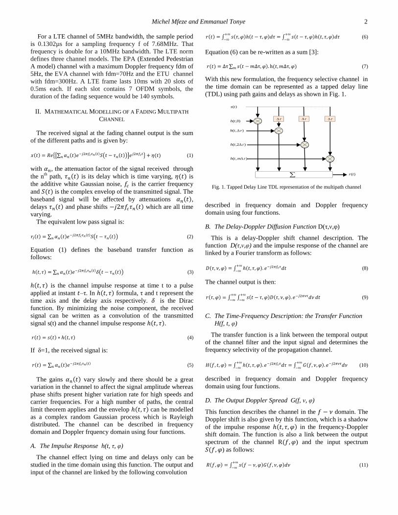
Equation (6) can be re-written as a sum [3]:
(7)
With this new formulation, the frequency selective channel in
the time domain can be represented as a tapped delay line
(TDL) using path gains and delays as shown in Fig. 1.
Fig. 1. Tapped Delay Line TDL representation of the multipath channel
described in frequency domain and Doppler frequency
domain using four functions.
B. The Delay-Doppler Diffusion Function D(τ,ν,φ)
This is a delay-Doppler shift channel description. The
function D(τ,ν,φ) and the impulse response of the channel are
linked by a Fourier transform as follows:
(8)
The channel output is then:
(9)
C. The Time-Frequency Description: the Transfer Function
H(f, t, φ)
The transfer function is a link between the temporal output
of the channel filter and the input signal and determines the
frequency selectivity of the propagation channel.
(10)
described in frequency domain and Doppler frequency
domain using four functions.
D. The Output Doppler Spread G(f, ν, φ)
This function describes the channel in the domain. The
Doppler shift is also given by this function, which is a shadow
of the impulse response in the frequency-Doppler
shift domain. The function is also a link between the output
spectrum of the channel R ) and the input spectrum
) as follows:
(11)
. . .
)(ts
)(tr
)0,(th
),( th
)2,( th
),( mth
International Journal of Computer Science and Telecommunications [Volume 6, Issue 11, December 2015] 3
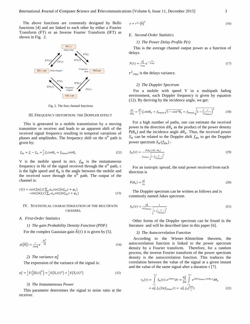
The above functions are commonly designed by Bello
functions [4] and are linked to each other by either a Fourier
Transform (FT) or an Inverse Fourier Transform (IFT) as
shown in Fig. 2.
Fig. 2. The four channel functions
III. FREQUENCY DISTORTION: THE DOPPLER EFFECT
This is generated in a mobile transmission by a moving
transmitter or receiver and leads to an apparent shift of the
received signal frequency resulting in temporal variations of
phases and amplitudes. The frequency shift on the nth
path is
given by:
(12)
V is the mobile speed in m/s. is the instantaneous
frequency in Hz of the signal received through the nth
path, c
is the light speed and is the angle between the mobile and
the received wave through the nth
path. The output of the
channel is:
(13)
IV. STATISTICAL CHARACTERIZATION OF THE MULTIPATH
CHANNEL
A. First-Order Statistics
1) The gain Probability Density Function (PDF)
For the complex Gaussian gain it is given by [5].
(14)
2) The variance
The expression of the variance of the signal is:
(15)
3) The Instantaneous Power
This parameter determines the signal to noise ratio at the
receiver.
= (16)
E. Second-Order Statistics
1) The Power Delay Profile P(τ)
This is the average channel output power as a function of
delays.
(17)
is the delays variance.
2) The Doppler Spectrum
For a mobile with speed V in a multipath fading
environment, each Doppler frequency is given by equation
(12). By deriving by the incidence angle, we get:
(18)
For a high number of paths, one can estimate the received
power in the direction as the product of the power density
P( ) and the incidence angle . Thus, the received power
can be related to the Doppler shift to get the Doppler
power spectrum :
(19)
For an isotropic spread, the total power received from each
direction is
(20)
The Doppler spectrum can be written as follows and is
commonly named Jakes spectrum.
(21)
Other forms of the Doppler spectrum can be found in the
literature and will be described later in this paper [6].
3) The Autocorrelation Function
According to the Wiener–Khintchine theorem, the
autocorrelation function is linked to the power spectrum
density by a Fourier transform. Therefore, for a random
process, the inverse Fourier transform of the power spectrum
density is the autocorrelation function. This traduces the
correlation between the value of the signal at a given instant
and the value of the same signal after a duration τ [7].
(22)
G(f,ν,φ)
h( ,t,
φ)
D( ,ν,φ)
)(IFT f
)(tFT
)(IFT f
)(tFT
)(IFT)(FT
)(IFT
)(FT
H(f,t,φ) Frequency-
Time
Frequency-
Doppler
Delay-Doppler
Delay-Time
Michel Mfeze and Emmanuel Tonye 4
It can be seen that the autocorrelation depends on the time
delay τ and the spatial shift . The k-order autocorrelation
coefficient is given by:
(23)
with
et
The most important is .
4) The Level Crossing Rate
The level crossing rate is a metric of the fading speed and
quantify how many times the signal crosses a given threshold
ρ in the positive direction. The following formulation is
derived from the classical Doppler spectrum.
(24)
is the threshold normalized by the root mean square (RMS)
of the signal and is the maximum Doppler spectrum.
5) The Average Fade Duration
The average fade duration is the average time the signal is
lower than or equal to a given threshold . It is also the
average time between two successive level crossing in both
directions (negative and positive). The formulation below
results from the classical Doppler spectrum.
(25)
F. Types of Doppler Spectra
1) Jakes Classical Doppler Spectrum
The Jakes Doppler spectrum is given by [6], [8]:
(26)
2) Flat Doppler Spectrum
(7)
3) Asymetric Jakes Doppler Spectrum
(28)
with
4) Bell Doppler Spectrum
(29)
Where a0, a2, and a4 are real and are the polynomial
coefficients of the spectrum.
5) Gaussian Doppler Spectrum
(30)
Where with the standard deviation of the
Gaussian classical function.
6) Bi-Gaussian Doppler Spectrum
(31)
g1 and g2 are the power gains of the Gaussian components
with values following a linear scale. fc1 and fc2 represent the
central frequencies of the Gaussian components normalized
by the maximum Doppler frequency. Values are therefore
within interval [-1,1]. Finally are real positive and are
the standard deviation of the Gaussian function normalized by
the maximum Doppler frequency.
f) The Laplacian Doppler Spectrum
(32)
7) The SUI (Stanford University Interim ) Doppler
Spectrum
(33)
8) The 3GPP-Rice Doppler Spectrum
(34)
V. THE FILTERED WHITE GAUSSIAN NOISE METHOD
Let be the frequency response of a filter and a
signal with power spectral density being filtered. The
power spectral density of the output signal is
given by:
(35)
International Journal of Computer Science and Telecommunications [Volume 6, Issue 11, December 2015] 5
In order to generate In- phase and quadrature components
of the channel complex coefficients, each having a Doppler
spectrum , one needs to filter white Gaussian
noise with power spectral density through a filter with frequency response
(36)
The above filter can be implemented either by Inverse
Discrete Fourier Transform (IFDT) or by a regressive filter
[5].
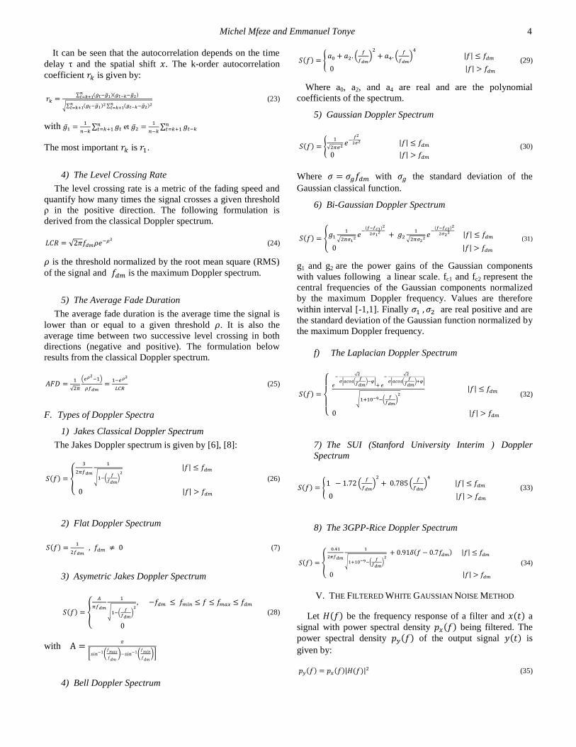
A. The Smith’s Model
Smith [9] used in-phase I and quadrature Q components
concept to simulate Clarke and Gans fading model. This is a
translation of equation (3) as shown in Fig. 3.
Fig. 3. Clarke and Gans model
Two Gaussian noise sources g1 and g2 are used to generate I
and Q. Each component is a sum of two real and orthogonal
random Gaussian independent variables, a and b. The
resulting variable g=a+jb is therefore Gaussian complex. The
Jakes Doppler spectrum is then used as a filter. The IFDT is
used at the end of the model for frequency domain signal
shaping to get time domain precise waves forms [10]. Each
Smith noise source is a random Gaussian complex number
generator of length Nrv and produces a baseband spectral line
with complex weights in the positive frequency band. The
spectral line is bounded either side by the maximum Doppler
frequency [ ] with equally distributed components
along the line. The negative components are the conjugates of
the Gaussian complex values for positive frequencies. In order
to get correlated signals, the random variables of the spectral
line are then multiplied by a discrete frequency representation
of with same length as the noise source. Each filter
output is then passed through an Inverse Fast Fourier
Transform (IFFT) module and finally the channel output is
computed as the sum of the two IFFT modules output.
Smith solved the problem of infinity approach at the limit
of bandwidth by truncating then increasing the slope
before that limit. The scheme on Fig. 4. shows the Smith’s
simulation model which is a frequency domain representation
of the above model, much easier to implement.
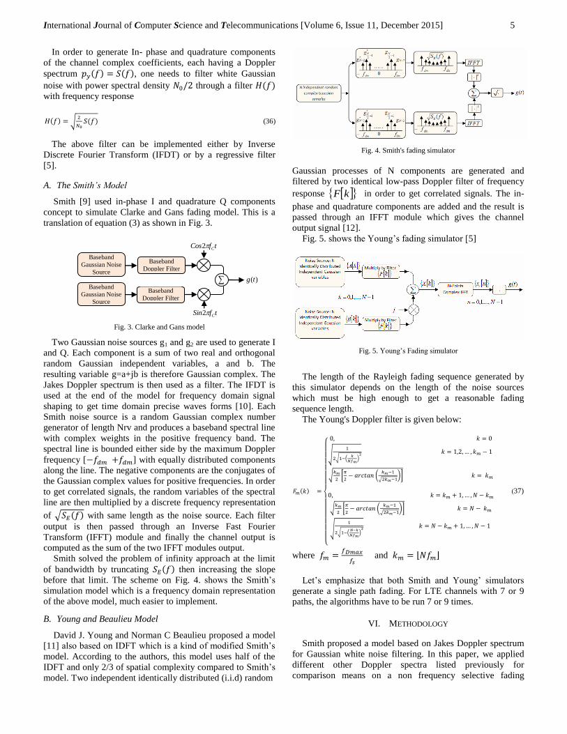
B. Young and Beaulieu Model
David J. Young and Norman C Beaulieu proposed a model
[11] also based on IDFT which is a kind of modified Smith’s
model. According to the authors, this model uses half of the
IDFT and only 2/3 of spatial complexity compared to Smith’s
model. Two independent identically distributed (i.i.d) random
Fig. 4. Smith's fading simulator
Gaussian processes of N components are generated and
filtered by two identical low-pass Doppler filter of frequency
response kF in order to get correlated signals. The in-
phase and quadrature components are added and the result is
passed through an IFFT module which gives the channel
output signal [12].
Fig. 5. shows the Young’s fading simulator [5]
Fig. 5. Young’s Fading simulator
The length of the Rayleigh fading sequence generated by
this simulator depends on the length of the noise sources
which must be high enough to get a reasonable fading
sequence length.
The Young's Doppler filter is given below:
(37)
where
and
Let’s emphasize that both Smith and Young’ simulators
generate a single path fading. For LTE channels with 7 or 9
paths, the algorithms have to be run 7 or 9 times.
VI. METHODOLOGY
Smith proposed a model based on Jakes Doppler spectrum
for Gaussian white noise filtering. In this paper, we applied
different other Doppler spectra listed previously for
comparison means on a non frequency selective fading
Baseband
Doppler Filter
Baseband
Gaussian Noise
Source
Baseband
Gaussian Noise
Source
tfCos C2
tfSin C2
)(tg
Baseband
Doppler Filter
Michel Mfeze and Emmanuel Tonye 6
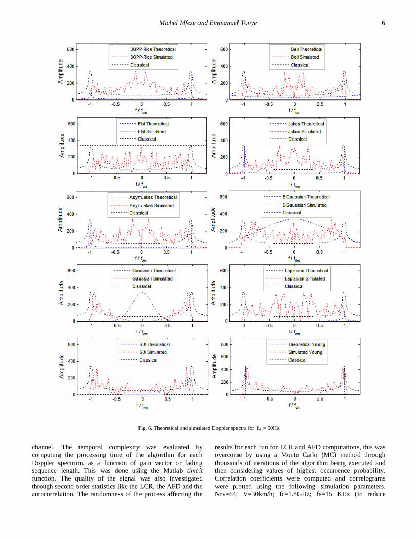
Fig. 6. Theoretical and simulated Doppler spectra for fdm= 50Hz
channel. The temporal complexity was evaluated by
computing the processing time of the algorithm for each
Doppler spectrum, as a function of gain vector or fading
sequence length. This was done using the Matlab timeit
function. The quality of the signal was also investigated
through second order statistics like the LCR, the AFD and the
autocorrelation. The randomness of the process affecting the
results for each run for LCR and AFD computations, this was
overcome by using a Monte Carlo (MC) method through
thousands of iterations of the algorithm being executed and
then considering values of highest occurrence probability.
Correlation coefficients were computed and correlograms
were plotted using the following simulation parameters.
Nrv=64; V=30km/h; fc=1.8GHz; fs=15 KHz (to reduce
International Journal of Computer Science and Telecommunications [Volume 6, Issue 11, December 2015] 7
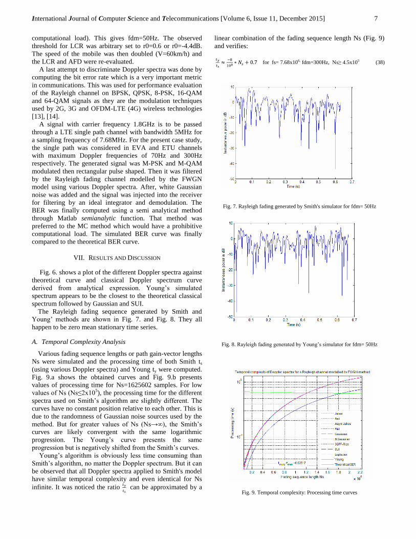
computational load). This gives fdm=50Hz. The observed
threshold for LCR was arbitrary set to r0=0.6 or r0=-4.4dB.
The speed of the mobile was then doubled (V=60km/h) and
the LCR and AFD were re-evaluated.
A last attempt to discriminate Doppler spectra was done by
computing the bit error rate which is a very important metric
in communications. This was used for performance evaluation
of the Rayleigh channel on BPSK, QPSK, 8-PSK, 16-QAM
and 64-QAM signals as they are the modulation techniques
used by 2G, 3G and OFDM-LTE (4G) wireless technologies
[13], [14].
A signal with carrier frequency 1.8GHz is to be passed
through a LTE single path channel with bandwidth 5MHz for
a sampling frequency of 7.68MHz. For the present case study,
the single path was considered in EVA and ETU channels
with maximum Doppler frequencies of 70Hz and 300Hz
respectively. The generated signal was M-PSK and M-QAM
modulated then rectangular pulse shaped. Then it was filtered
by the Rayleigh fading channel modelled by the FWGN
model using various Doppler spectra. After, white Gaussian
noise was added and the signal was injected into the receiver
for filtering by an ideal integrator and demodulation. The
BER was finally computed using a semi analytical method
through Matlab semianalytic function. That method was
preferred to the MC method which would have a prohibitive
computational load. The simulated BER curve was finally
compared to the theoretical BER curve.
VII. RESULTS AND DISCUSSION
Fig. 6. shows a plot of the different Doppler spectra against
theoretical curve and classical Doppler spectrum curve
derived from analytical expression. Young’s simulated
spectrum appears to be the closest to the theoretical classical
spectrum followed by Gaussian and SUI.
The Rayleigh fading sequence generated by Smith and
Young’ methods are shown in Fig. 7. and Fig. 8. They all
happen to be zero mean stationary time series.
A. Temporal Complexity Analysis
Various fading sequence lengths or path gain-vector lengths
Ns were simulated and the processing time of both Smith ts
(using various Doppler spectra) and Young ty were computed.
Fig. 9.a shows the obtained curves and Fig. 9.b presents
values of processing time for Ns=1625602 samples. For low
values of Ns (Ns≤2x10⁵), the processing time for the different
spectra used on Smith’s algorithm are slightly different. The
curves have no constant position relative to each other. This is
due to the randomness of Gaussian noise sources used by the
method. But for greater values of Ns (Ns→∞), the Smith’s
curves are likely convergent with the same logarithmic
progression. The Young’s curve presents the same
progression but is negatively shifted from the Smith’s curves.
Young’s algorithm is obviously less time consuming than
Smith’s algorithm, no matter the Doppler spectrum. But it can
be observed that all Doppler spectra applied to Smith's model
have similar temporal complexity and even identical for Ns
infinite. It was noticed the ratio
can be approximated by a
linear combination of the fading sequence length Ns (Fig. 9)
and verifies:
for fs= 7.68x10⁶, fdm=300Hz, Ns≥ 4.5x10⁵ (38)
Fig. 7. Rayleigh fading generated by Smith's simulator for fdm= 50Hz
Fig. 8. Rayleigh fading generated by Young’s simulator for fdm= 50Hz
Fig. 9. Temporal complexity: Processing time curves
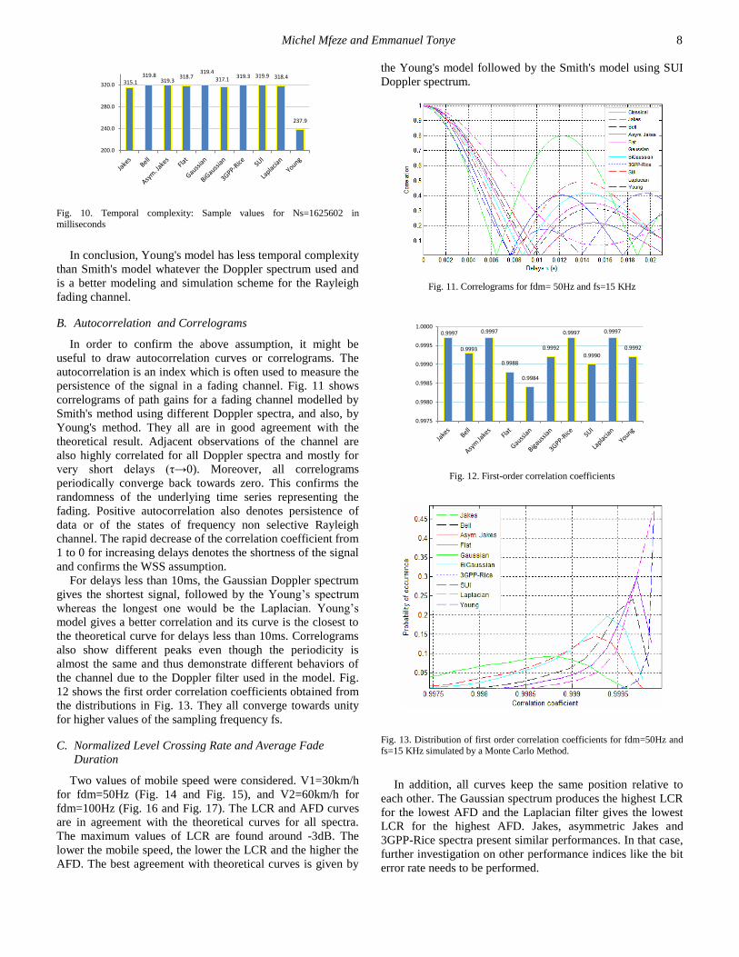
Michel Mfeze and Emmanuel Tonye 8
Fig. 10. Temporal complexity: Sample values for Ns=1625602 in
milliseconds
In conclusion, Young's model has less temporal complexity
than Smith's model whatever the Doppler spectrum used and
is a better modeling and simulation scheme for the Rayleigh
fading channel.
B. Autocorrelation and Correlograms
In order to confirm the above assumption, it might be
useful to draw autocorrelation curves or correlograms. The
autocorrelation is an index which is often used to measure the
persistence of the signal in a fading channel. Fig. 11 shows
correlograms of path gains for a fading channel modelled by
Smith's method using different Doppler spectra, and also, by
Young's method. They all are in good agreement with the
theoretical result. Adjacent observations of the channel are
also highly correlated for all Doppler spectra and mostly for
very short delays (τ→0). Moreover, all correlograms
periodically converge back towards zero. This confirms the
randomness of the underlying time series representing the
fading. Positive autocorrelation also denotes persistence of
data or of the states of frequency non selective Rayleigh
channel. The rapid decrease of the correlation coefficient from
1 to 0 for increasing delays denotes the shortness of the signal
and confirms the WSS assumption.
For delays less than 10ms, the Gaussian Doppler spectrum
gives the shortest signal, followed by the Young’s spectrum
whereas the longest one would be the Laplacian. Young’s
model gives a better correlation and its curve is the closest to
the theoretical curve for delays less than 10ms. Correlograms
also show different peaks even though the periodicity is
almost the same and thus demonstrate different behaviors of
the channel due to the Doppler filter used in the model. Fig.
12 shows the first order correlation coefficients obtained from
the distributions in Fig. 13. They all converge towards unity
for higher values of the sampling frequency fs.
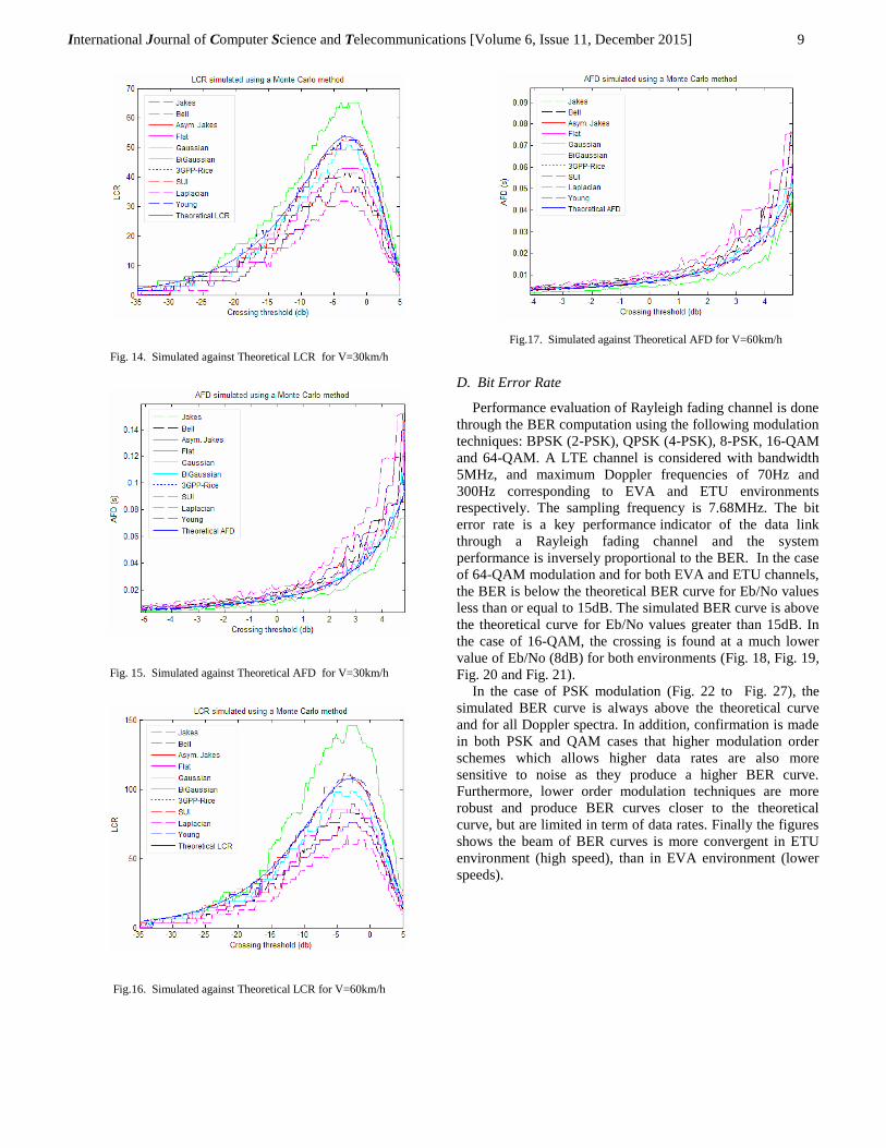
C. Normalized Level Crossing Rate and Average Fade
Duration
Two values of mobile speed were considered. V1=30km/h
for fdm=50Hz (Fig. 14 and Fig. 15), and V2=60km/h for
fdm=100Hz (Fig. 16 and Fig. 17). The LCR and AFD curves
are in agreement with the theoretical curves for all spectra.
The maximum values of LCR are found around -3dB. The
lower the mobile speed, the lower the LCR and the higher the
AFD. The best agreement with theoretical curves is given by
the Young's model followed by the Smith's model using SUI
Doppler spectrum.
Fig. 11. Correlograms for fdm= 50Hz and fs=15 KHz
Fig. 12. First-order correlation coefficients
Fig. 13. Distribution of first order correlation coefficients for fdm=50Hz and
fs=15 KHz simulated by a Monte Carlo Method.
In addition, all curves keep the same position relative to
each other. The Gaussian spectrum produces the highest LCR
for the lowest AFD and the Laplacian filter gives the lowest
LCR for the highest AFD. Jakes, asymmetric Jakes and
3GPP-Rice spectra present similar performances. In that case,
further investigation on other performance indices like the bit
error rate needs to be performed.
315.1 319.8
319.3 318.7
319.4 317.1
319.3 319.9 318.4
237.9
200.0
240.0
280.0
320.0
0.9997
0.9993
0.9997
0.9988
0.9984
0.9992
0.9997
0.9990
0.9997
0.9992
0.9975
0.9980
0.9985
0.9990
0.9995
1.0000
International Journal of Computer Science and Telecommunications [Volume 6, Issue 11, December 2015] 9
Fig. 14. Simulated against Theoretical LCR for V=30km/h
Fig. 15. Simulated against Theoretical AFD for V=30km/h
Fig.16. Simulated against Theoretical LCR for V=60km/h
Fig.17. Simulated against Theoretical AFD for V=60km/h
D. Bit Error Rate
Performance evaluation of Rayleigh fading channel is done
through the BER computation using the following modulation
techniques: BPSK (2-PSK), QPSK (4-PSK), 8-PSK, 16-QAM
and 64-QAM. A LTE channel is considered with bandwidth
5MHz, and maximum Doppler frequencies of 70Hz and
300Hz corresponding to EVA and ETU environments
respectively. The sampling frequency is 7.68MHz. The bit
error rate is a key performance indicator of the data link
through a Rayleigh fading channel and the system
performance is inversely proportional to the BER. In the case
of 64-QAM modulation and for both EVA and ETU channels,
the BER is below the theoretical BER curve for Eb/No values
less than or equal to 15dB. The simulated BER curve is above
the theoretical curve for Eb/No values greater than 15dB. In
the case of 16-QAM, the crossing is found at a much lower
value of Eb/No (8dB) for both environments (Fig. 18, Fig. 19,
Fig. 20 and Fig. 21).
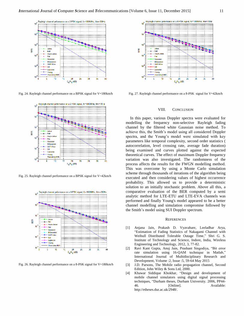
In the case of PSK modulation (Fig. 22 to Fig. 27), the
simulated BER curve is always above the theoretical curve
and for all Doppler spectra. In addition, confirmation is made
in both PSK and QAM cases that higher modulation order
schemes which allows higher data rates are also more
sensitive to noise as they produce a higher BER curve.
Furthermore, lower order modulation techniques are more
robust and produce BER curves closer to the theoretical
curve, but are limited in term of data rates. Finally the figures
shows the beam of BER curves is more convergent in ETU
environment (high speed), than in EVA environment (lower
speeds).
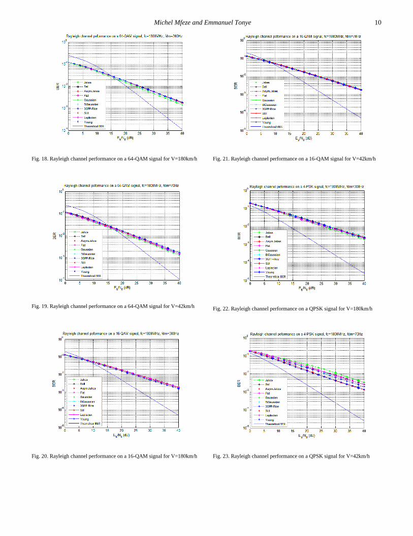
Michel Mfeze and Emmanuel Tonye 10
Fig. 18. Rayleigh channel performance on a 64-QAM signal for V=180km/h
Fig. 19. Rayleigh channel performance on a 64-QAM signal for V=42km/h
Fig. 20. Rayleigh channel performance on a 16-QAM signal for V=180km/h
Fig. 21. Rayleigh channel performance on a 16-QAM signal for V=42km/h
Fig. 22. Rayleigh channel performance on a QPSK signal for V=180km/h
Fig. 23. Rayleigh channel performance on a QPSK signal for V=42km/h
International Journal of Computer Science and Telecommunications [Volume 6, Issue 11, December 2015] 11
Fig. 24. Rayleigh channel performance on a BPSK signal for V=180km/h
Fig. 25. Rayleigh channel performance on a BPSK signal for V=42km/h
Fig. 26. Rayleigh channel performance on a 8-PSK signal for V=180km/h
Fig. 27. Rayleigh channel performance on a 8-PSK signal for V=42km/h
VIII. CONCLUSION
In this paper, various Doppler spectra were evaluated for
modelling the frequency non-selective Rayleigh fading
channel by the filtered white Gaussian noise method. To
achieve this, the Smith’s model using all considered Doppler
spectra, and the Young’s model were simulated with key
parameters like temporal complexity, second order statistics (
autocorrelation, level crossing rate, average fade duration)
being examined and curves plotted against the expected
theoretical curves. The effect of maximum Doppler frequency
variation was also investigated. The randomness of the
process affects the results for the FWGN modelling method.
This was overcome by using a Monte Carlo simulation
scheme through thousands of iterations of the algorithm being
executed and then considering values of highest occurrence
probability. This allowed us to provide a deterministic
solution to an initially stochastic problem. Above all this, a
comparative evaluation of the BER computed by a semi
analytic method for LTE-ETU and LTE-EVA channels was
performed and finally Young's model appeared to be a better
channel modelling and simulation compromise followed by
the Smith’s model using SUI Doppler spectrum.
REFERENCES
[1] Anjana Jain, Prakash D. Vyavahare, Leeladhar Arya,
“Estimation of Fading Statistics of Nakagami Channel with
Weibull Distributed Tolerable Outage Time,” Shri G. S.
Institute of Technology and Science, Indore, India, Wireless
Engineering and Technology, 2012, 3, 77-82.
[2] Ravi Kant Gupta, Anuj Jain, Prashant Singodiya, “Bit error
rate simulation using 16-QAM technique in Matlab,”
International Journal of Multidisciplinary Research and
Development, Volume :2, Issue :5, 59-64 May 2015
[3] J.D. Parsons, The Mobile radio propagation channel, Second
Edition, John Wiley & Sons Ltd, 2000.
[4] Khawar Siddique Khokhar, “Design and development of
mobile channel simulators using digital signal processing
techniques, “Durham theses, Durham University. 2006, PP44-
46. [Online]. Available:
http://etheses.dur.ac.uk/2948/.
Michel Mfeze and Emmanuel Tonye 12
[5] Ali Arsal, “A study on wireless channel models: Simulation of
fading, shadowing and further applications, ” M. Eng. thesis,
Izmir Institute of Technology. August 2008.
[6] Yong Soo Cho, Jaekwon Kim, Won Young Yang, Chung G.
Kang, MIMO-OFDM wireless communications with
MATLAB, Ed John Wiley & Sons (Asia) Pte Ltd, 2010.
[7] Ahmed Saadani, Méthodes de Simulations Rapides du Lien
Radio pour les Systèmes 3G, Thèse de Doctorat, Ecole
Nationale Supérieure de Paris, Décembre 2003.
[8] Cyril-Daniel Iskander, “ A MATLAB -based Object-Oriented
Approach to Multipath Fading Channel Simulation,” Hi-Tek
Multisystems, Québec, QC, Canada, G1H 3V9.
[9] John I. Smith, “ A Computer Generated Multipath Fading
Simulation for Mobile Radio,” IEEE Transactions on
Vehicular Technology, vol VT-24, No. 3, August 1975.
[10] Theodore S. Rappaport, Wireless Communications: Principles
and Practice (2nd Edition), Ed Prentice Hall, 2002.
[11] David J. Young and Norman C. Beaulieu, “ The generation of
correlated Rayleigh random variates by inverse discrete
Fourier transform,” IEEE transactions on Communications,
vol. 48, pp. 1114-1127, July 2000.
[12] Abdellah Berdai, “ Egalisation aveugle et turbo égalisation
dans les canaux sélectifs en fréquence invariants et variant
dans le temps, ” Mémoire de maîtrise en génie électrique.
Université Laval. Québec, 2006.
[13] Houman Zarrinkoub, Understanding LTE with Matlab. From
mathematical modelling to simulation and prototyping, Ed
John Wiley & Sons Ltd, 2014.
[14] Yannick Bouguen, Éric Hardouin, François-Xavier Wolff, LTE
et les réseaux 4G, Sous la direction de Guy Pujolle, Editions
Groupe Eyrolles, 2012 Chapitre 1.