Article

Comparative Analysis of the Impact of AdditivelyManufactured Polymer Tools on the FiberConfiguration of Injection MoldedLong-Fiber-Reinforced Thermoplastics

Lukas Knorr 1,2,*,† , Robert Setter 3,† , Dominik Rietzel 2, Katrin Wudy 3 and Tim Osswald 4

1 Institute of Polymer Technology, University of Erlangen-Nuremberg, 91058 Erlangen, Germany2 Department of Additive Manufacturing, BMW Group, 85764 Oberschleissheim, Germany;

Dominik.Rietzel@bmw.de3 Department of Mechanical Engineering, Professorship of Laser-Based Additive Manufacturing,

Technical University of Munich, 85748 Munich, Germany; robert.setter@tum.de (R.S.);katrin.wudy@tum.de (K.W.)

4 Mechanical Engineering Department, Polymer Engineering Center, University of Wisconsin-Madison,Madison, WI 53706, USA; tosswald@wisc.edu

* Correspondence: knorr.lukas@gmx.de† Contributed equally to this work.

Received: 7 August 2020; Accepted: 11 September 2020; Published: 15 September 2020�����������������

Abstract: Additive tooling (AT) utilizes the advantages of rapid tooling development while minimizinggeometrical limitations of conventional tool manufacturing such as complex design of cooling channels.This investigation presents a comparative experimental analysis of long-fiber-reinforced thermoplasticparts (LFTs), which are produced through additively manufactured injection molding polymer tools.After giving a review on the state of the art of AT and LFTs, additive manufacturing (AM) plastic toolsare compared to conventionally manufactured steel and aluminum tools toward their qualificationfor spare part and small series production as well as functional validation. The assessment of thepolymer tools focuses on three quality criteria concerning the LFT parts: geometrical accuracy,mechanical properties, and fiber configuration. The analysis of the fiber configuration includesfiber length, fiber concentration, and fiber orientation. The results show that polymer tools are fullycapable of manufacturing LFTs with a cycle number within hundreds before showing critical signs ofdeterioration or tool failure. The produced LFTs moldings provide sufficient quality in geometricalaccuracy, mechanical properties, and fiber configuration. Further, specific anomalies of the fiberconfiguration can be detected for all tool types, which include the occurrence of characteristic zonesdependent on the nominal fiber content and melt flow distance. Conclusions toward the improvementof additively manufactured polymer tool life cycles are drawn based on the detected deteriorationsand failure modes.

Keywords: additive tooling; additive manufacturing; rapid tooling; injection molding;polypropylene; long-fiber-reinforced thermoplastics; fiber length; fiber orientation; fiberconcentration; stereolithography

1. Introduction

1.1. Motivation

In the most recent decades, the ease of processability of long-fiber-reinforced thermoplastics (LFT)has enabled their use as advanced lightweight engineering materials, particularly within the automotive

J. Compos. Sci. 2020, 4, 136; doi:10.3390/jcs4030136 www.mdpi.com/journal/jcs

J. Compos. Sci. 2020, 4, 136 2 of 32

sector [1,2]. As a key technology, the injection molding process is expected to take a major role in termsof value and volume [3]. With an estimated market volume percentage of 65%, polypropylene (PP) isthe material with the biggest market volume of LFTs in this field [4]. Material glass is predominantlyused for reinforcement due to its low cost and superior mechanical properties [5].

Additive manufacturing (AM) is becoming increasingly important in industry in general and isbecoming especially important in the automotive sector [6]. Although a lot of research and developmentis carried out, AM is still very limited in its available range of materials, which prevents its widespreadentry into large-scale industry [7]. Due to its generative layer structure, most of the materials showlower molecular cohesion in one or more load directions [8]. Consequently, anisotropic materialproperties that deviate from those of the injection molded (IM) pedant must be expected [9]. This countsparticularly for polymers; therefore, commodity construction materials such as PP, PU, PA, PC, blends,and other compounds can only be substituted to a very limited amount [10].

Additive tooling (AT) describes a process which combines the potential of AM with the materialspectrum of a traditional manufacturing process, such as IM, by replacing the molding tool unit byan additive one and keeping the existing equipment of the traditional manufacturing technologyalive. In this way, it is possible to produce moldings with series properties, to reduce the cost andtime-consuming tool manufacturing process, and to increase the tooling complexity and the resultingpart design freedom at the same time [11,12]. For this procedure, polymer molds are currently preferreddue to their superior surface quality, lower production time, and lower costs in comparison to its metalpedant [13]. For AT, the most important production method is stereolithography (SL), which providessupreme surfaces with a high geometrical accuracy and the access to cross-linked and reinforcedpolymers. These composites are based on a high-temperature resistant polymer matrix which isenhanced with fillers such as aluminum or ceramics particles to improve the thermal conductivity,heat deflection point, and mechanical properties [14,15]. In general, plastic molds show a significantdeviation from the conventional steel tools in points of heat capacity as well as in their temperatureand thermal conductivity around a factor of 10 to 100 [16]. As the properties and behavior of plasticcomponents are mainly defined by their thermal history, the cooling process of the polymer tools iscrucial for the morphology and the crystallization of the moldings.

The objective of this investigation is to qualify additively manufactured polymer tools for thefabrication of LFT parts for functional validation, spare parts, and small series production. For thispurpose, the effects of three different tool materials (ceramic reinforced plastic, steel, and aluminum) onthe process-induced fiber configuration are investigated and compared with each other. The iterativetool design process is performed for all materials individually and is based on Moldflow simulationsand basic principles of heat transfer. Especially in terms of the cooling systems, the advantages ofAT are specifically implemented. Representative for the most used LFT, the glass fiber-reinforcedPP injection molding material STAMAX™ from SABIC is used in different fiber weight percentages.Tensile specimens and discs are used as sample geometries to map both a linear and a radial source flow.The process-induced fiber configuration is investigated over the flow path and over the componentthickness. The central injection point at the disc mold will also allow investigation of the transitionfrom a swirling to a pointed flow. Furthermore, the impact of the different tool materials on significantmechanical properties of the fiber-reinforced moldings are analyzed. For the test methods, CT scan,pyrolysis, tensile testing, and a fiber length measurement method modeled after that of Goris et al. [17]are carried out. To evaluate the economic efficiency, the tool life and the suitability of AT will beassessed on the degree of wear, defect patterns, and output quantity.

1.2. State of the Art

AM is ideally used to manufacture components directly without using the indirect process chainof AT. For this purpose, there are many commercially available fabrication methods (i.e., fused filamentfabrication (FFF), selective laser sintering (SLS), and multi jet fusion) and materials that contain fiberreinforcements. However, their properties are not comparable with IM materials and especially

J. Compos. Sci. 2020, 4, 136 3 of 32

not with LFTs due to their short fiber character and diverging fiber configuration. The commoditypolymer PP is well known for its difficulty in processing within AM due to its shrinkage and lowadhesion. Nevertheless, Sodeifian et al. [18] achieved good processing results of PP/GF with theadditive POE-g-MA on a FFF platform. Still, the material is lagging behind in its mechanical propertiesand is deviating strongly from its compression molding pedant by 30%. To fabricate classic IM materialsdirectly, another promising approach arose in the most recent decades. It is a modified FFF methodwhere the filament extruder is exchanged for a granulate-fed portable extruder unit. On that base,Hertle et al. [19] achieved good results by melt extrusion of PP injection molding granulate. Thoughit was unlikely, the process suffers the same issue of an insufficient interlaminar bonding, whichis strongly incoherent compared to the intralaminar ones and is leading into anisotropic materialproperties [20].

AT is the indirect process chain and a tool-bound alternative, which allows it to maintain theoriginal manufacturing process and its material variety. Kampker et al. [21], investigated the suitabilityof polyjet (PJ), SL, digital light synthesis (DLS), and SLS processes for direct IM tool production.The investigations showed that the material PA 3200 GF is the most suitable for SLS, while for the SLmethod, composite materials such as Accura® Bluestone™ and Perform are the most promising ones.Rahmati and Dickens [22] examined the output of SL produced tools in the field of IM. They achievedan output of more than 500 parts and found that the main tool failure was due to flexural and excessivefriction. Hofstätter et al. [23] achieved the same results.

For the improvement of the part properties, as well as the extension of the tool life and to decreasethe cycle time, extensive research is being done on optimized cooling systems and adapted processparameters. Altaf et al. [24] demonstrate the general effectiveness of a conformal cooling system in adirect comparison with a conventional cooling design. In this example, the conformal cooling systemleads to a cycle time reduction of approx. 20%. The investigations of Park et al. [25] show even betterperformances of up to 30%, whereby only tool areas relevant to the cycle time are replaced by SLM(Selective Laser Melting) inserts with a conformal cooling unit. However, Hopkins et al. [26] observedin a direct comparison of an aluminum and a polymer IM tool an increased cycle time and significantdifferences in the rheology of the injection molding material. The lower thermal conductivity of themold materials results into longer flow paths, which in turn requires lower process pressures and melttemperatures. In earlier investigations of Martinho et al. [27], the influence on the morphology ofsemi-crystalline PP moldings is revealed in a direct comparison of an epoxy and steel mold material.As soon as different materials were used for core and cavity, a clear asymmetrical crystalline structurewas observed. In concerns of the influence on the material properties of the moldings, the investigationsof Harris et al. [28,29] should be emphasized. He states that with the aid of a modified cooling systemand the adaptation of the necessary process parameters, the crystallinity can be strongly influenced,even to the extent that comparable part properties can be achieved using polymer and CNC milledsteel/aluminum molds. Similar results were achieved by Fernandes et al. [30] and Volpato et al. [31].Recent investigations by Kampkar et al. [16] proved that the materials still show a rather brittle andnon-ductile fracture behavior. However, the deviations can be attributed with high probability toparticle agglomeration due to the lower thermal conductivity and a greater surface roughness.

On the side of LFTs, the investigations of Kim et al. [32] show that the mechanical and the impactstrength increases with the fiber length. Furthermore, they measured a reduction of the initial fiberlength of 4–16 mm to a residual fiber length of about 0.5–2 mm during processing. The results areconsistent with Seong et al. [33], who noted an increase in Young’s modulus, melting temperature,and viscoelastic properties, and a less uniform distribution of the fiber with an increasing fiber length.Hou et al. [34] measured a reduction of the average fiber length with an increasing injection rate overthe whole length of tensile specimens. Based on the work of Tadmor [35] as well as Osswald andMenges [36], there are seven characteristic regions that can be differentiated in injection molded parts,each with a specific fiber orientation. The two skin layers provide random fiber orientation, whilethe shell layers are aligned parallel to the melt flow direction. The fiber alignment of the core layer

J. Compos. Sci. 2020, 4, 136 4 of 32

is perpendicular to the melt flow direction, with two randomly oriented transition layers betweenthe core layer and the shell layers. This specific orientation pattern is well-known and caused by thefountain flow effect. However, the numerical predictions of Hou et al. [34] do not match with theempirical orientation in the skin layer. Parveen et al. [37] achieved comparable results to Hou et al. ona disc geometry (2 mm; 75 mm D) and stated that a higher fiber length leads to a wider core regionwith more fibers aligned transverse to the flow direction at the end of the flow path. Zhu et al. [38]compared a centered and an end-gated injecting model. It is found that the end-gated plate has a moredefined shell area of 55%, where the fibers align along the main flow direction and a core region of20%, with fibers aligned perpendicular to it. The shell area of the center-gated plates takes a 35% andthe core area 35% at an equal density and fiber weight content. Goris et al. [17] detected a substantialincrease in fiber length along the flow path, which is probably due to a fiber pullout effect. The samecould be observed by Lafranche et al. [39], who detected a strong influence of the used gate typein addition. Furthermore, Goris [17] demonstrated in a comparative study that the so-called epoxyplug method, which is based on the investigations of Kunc et al. [40]. The new measurement methodis especially suitable for LFTs with a large sample size and can be used to generate accurate resultswith a strong repeatability while minimizing the manual handling effort. It is shown that the takenmeasurements agree with the outcome of previously reported studies [12,39,41]. Aside from the epoxyplug method, the comparative study concentrated on two other fiber analysis methods: first, a fullfiber analysis, which is a proprietary measurement system developed by SABIC (Geleen, Netherlands)and based on the work by Krasteva [42]; and second, the FASEP method, which is a commerciallyavailable analysis method proprietary to IDM Systems (Darmstadt, Germany).

For the analysis of the fiber orientation distribution, Sharma et al. [43] achieved sufficient resultswith a tensor-based marker watershed method. However, the method is relatively sensitive to impropersurface preparation and image processing techniques. A better application seems to be the evaluation ofindustrial micro-computed tomography (µCT) images. The fiber orientation is described in accordancewith the work of Adavani and Tucker [44], who assume that each fiber can be represented by aunit vector p spherical coordinates. The orientation is then described in tensor form. A schematicrepresentation can be seen in Figure 1 (left). Mathematically, the unit vector is described with theangles Φ, θ as:

p =

p1

p2

p3

=

cos(Φ)· sin(θ)sin(Φ)· sin(θ)

cos(θ)

(1)

The orientation tensor or Advani–Tucker tensor is calculated as:

αi j =

∮pi·p j·Ψ(p) dp (2)

While pi·p j is the product of the fiber orientation vector with itself, Ψ(p) represents a probabilityfunction of all possible orientations. This results in the following tensor components:

a11 =⟨sin2(Φ) cos2(θ)

⟩a12 =

⟨sin2(Φ) cos(θ) sin(θ)

⟩a13 =

⟨sin(Φ) cos(Φ) cos(θ)

⟩a21 = a12 a22 =

⟨sin2(Φ) sin2(θ)

⟩a23 =

⟨sin(Φ) cos(Φ) sin(θ)

⟩a31 = a13 a32 = a23 a33 =

⟨cos2(Φ)

⟩ (3)

Experimental data are conventionally illustrated using the orientation tensor form. The diagonalcomponents of the second order orientation tensor (a11, a22, and a33) describe the degree of orientationwith respect to the defined coordinate system. Conventionally, the reference coordinates are definedso that the 1-direction represents the inflow direction, the 2-direction is the crossflow direction andthe 3-direction is the thickness direction. The off-diagonal components of the orientation tensor showthe tilt of the orientation tensor from the coordinate axes. Hence, they are zero only if the coordinateaxes align with the principal directions of the orientation tensor [44]. Two examples for possible fiber

J. Compos. Sci. 2020, 4, 136 5 of 32

alignment are given in Figure 1. If completely random orientation occurs, the diagonal elements area11 = a22 = a33 = 1/3 (middle). For fiber orientation perpendicular to in-flow direction, the tensorelements are a11 = 0 a22 = 1 and a33 = 0 (right).

J. Compos. Sci. 2020, 4, x  5 of 32 

zero only if the coordinate axes align with the principal directions of the orientation tensor [44]. Two 

examples for possible fiber alignment are given in Figure 1. If completely random orientation occurs, 

the diagonal elements are  𝑎   =  𝑎   =  𝑎   = 1/3 (middle). For fiber orientation perpendicular to in‐

flow direction, the tensor elements are  𝑎   = 0  𝑎   = 1 and  𝑎   = 0 (right). 

 (a)  (b)  (c) 

Figure 1. Representation of the orientation of a single rigid fiber by the vector  𝒑(𝛷, 𝜃) (a) adapted after [44]; orientation of a fiber population within a volume: randomly oriented fibers (b) and aligned 

fibers (c), adapted after [36]. 

2. Materials and Methods 

2.1. Materials and Specimens 

2.1.1. Specimen Geometry and Mold Insert Design 

The specimen geometries used in this work are shown in Figure 2. The test specimen geometry 

for tensile tests according to DIN EN ISO 527 is based on the multipurpose specimen geometry 1A 

according to DIN EN ISO 527‐1 and DIN EN ISO 3167. For a high reproducibility of the specimen 

geometry, the cavity of the injection molding tool is flow‐optimized in deviation to DIN ISO 294‐1 to 

keep the wear of the AM tools as low as possible. The test specimen with its long flow path ratio is 

representative  for  a  linear  directed  flow  behavior. Due  to  the wall  thickness  of  4 mm,  a  good 

separation of a skin–shear–core–shear–skin orientation can be expected. The cavity and specimen 

geometry are shown in Figure 2. 

 

Figure 2. Melt flow path optimized tensile specimen geometry after DIN EN ISO 527 and DIN EN 

ISO 3167. 

For the investigation of the fiber configuration, a nonstandard disc with a thickness of 3 mm and 

a diameter of 120 mm is used. Due to the rotation symmetry of the disc, only a partial segment of the 

disc needs to be examined to draw conclusions about the entire test specimen. The central injection 

point at the disc mold will allow investigation of the transition from a swirling to a pointed flow. 

Likewise, a radial geometry provides an even pressure distribution during the IM process and thus 

reduces the process‐induced influence on the test specimens and measurement results. This plays an 

important role especially for AM tools, which tend to have a high deformation and mold breathing. 

12

3

12

3

p(𝜃, 𝛷)

𝛷

𝜃

1

2

3

Figure 1. Representation of the orientation of a single rigid fiber by the vector p(Φ, θ) (a) adaptedafter [44]; orientation of a fiber population within a volume: randomly oriented fibers (b) and alignedfibers (c), adapted after [36].

2. Materials and Methods

2.1. Materials and Specimens

2.1.1. Specimen Geometry and Mold Insert Design

The specimen geometries used in this work are shown in Figure 2. The test specimen geometryfor tensile tests according to DIN EN ISO 527 is based on the multipurpose specimen geometry 1Aaccording to DIN EN ISO 527-1 and DIN EN ISO 3167. For a high reproducibility of the specimengeometry, the cavity of the injection molding tool is flow-optimized in deviation to DIN ISO 294-1 tokeep the wear of the AM tools as low as possible. The test specimen with its long flow path ratio isrepresentative for a linear directed flow behavior. Due to the wall thickness of 4 mm, a good separationof a skin–shear–core–shear–skin orientation can be expected. The cavity and specimen geometry areshown in Figure 2.

J. Compos. Sci. 2020, 4, x  5 of 32 

zero only if the coordinate axes align with the principal directions of the orientation tensor [44]. Two 

examples for possible fiber alignment are given in Figure 1. If completely random orientation occurs, 

the diagonal elements are  𝑎   =  𝑎   =  𝑎   = 1/3 (middle). For fiber orientation perpendicular to in‐

flow direction, the tensor elements are  𝑎   = 0  𝑎   = 1 and  𝑎   = 0 (right). 

 (a)  (b)  (c) 

Figure 1. Representation of the orientation of a single rigid fiber by the vector  𝒑(𝛷, 𝜃) (a) adapted after [44]; orientation of a fiber population within a volume: randomly oriented fibers (b) and aligned 

fibers (c), adapted after [36]. 

2. Materials and Methods 

2.1. Materials and Specimens 

2.1.1. Specimen Geometry and Mold Insert Design 

The specimen geometries used in this work are shown in Figure 2. The test specimen geometry 

for tensile tests according to DIN EN ISO 527 is based on the multipurpose specimen geometry 1A 

according to DIN EN ISO 527‐1 and DIN EN ISO 3167. For a high reproducibility of the specimen 

geometry, the cavity of the injection molding tool is flow‐optimized in deviation to DIN ISO 294‐1 to 

keep the wear of the AM tools as low as possible. The test specimen with its long flow path ratio is 

representative  for  a  linear  directed  flow  behavior. Due  to  the wall  thickness  of  4 mm,  a  good 

separation of a skin–shear–core–shear–skin orientation can be expected. The cavity and specimen 

geometry are shown in Figure 2. 

 

Figure 2. Melt flow path optimized tensile specimen geometry after DIN EN ISO 527 and DIN EN 

ISO 3167. 

For the investigation of the fiber configuration, a nonstandard disc with a thickness of 3 mm and 

a diameter of 120 mm is used. Due to the rotation symmetry of the disc, only a partial segment of the 

disc needs to be examined to draw conclusions about the entire test specimen. The central injection 

point at the disc mold will allow investigation of the transition from a swirling to a pointed flow. 

Likewise, a radial geometry provides an even pressure distribution during the IM process and thus 

reduces the process‐induced influence on the test specimens and measurement results. This plays an 

important role especially for AM tools, which tend to have a high deformation and mold breathing. 

12

3

12

3

p(𝜃, 𝛷)

𝛷

𝜃

1

2

3

Figure 2. Melt flow path optimized tensile specimen geometry after DIN EN ISO 527 and DIN ENISO 3167.

For the investigation of the fiber configuration, a nonstandard disc with a thickness of 3 mm and adiameter of 120 mm is used. Due to the rotation symmetry of the disc, only a partial segment of the discneeds to be examined to draw conclusions about the entire test specimen. The central injection point atthe disc mold will allow investigation of the transition from a swirling to a pointed flow. Likewise,a radial geometry provides an even pressure distribution during the IM process and thus reduces theprocess-induced influence on the test specimens and measurement results. This plays an important

J. Compos. Sci. 2020, 4, 136 6 of 32

role especially for AM tools, which tend to have a high deformation and mold breathing. Furthermore,the disc geometry is frequently used in literature, so that the obtained results can be compared withexisting studies of Hongyu and Baird [45]. In the cases of Rohde et al. [46] and Goris et al. [17], whofocused more on a plate geometry, the results can be seen as complementary and further investigation.The cavity and specimen geometry are shown in Figure 3.

J. Compos. Sci. 2020, 4, x  6 of 32 

Furthermore, the disc geometry is frequently used in literature, so that the obtained results can be 

compared with existing studies of Hongyu and Baird [45]. In the cases of Rohde et al. [46] and Goris 

et al. [17], who  focused more on a plate geometry,  the results can be seen as complementary and 

further investigation. The cavity and specimen geometry are shown in Figure 3. 

 

Figure 3. Disc specimen geometry with a thickness of 3 mm and a diameter of 120 mm. 

2.1.2. Materials 

The AM tools are made from Accura Bluestone by the company 3D Systems®, which is processed 

on  a  Viper  si2  System  (SLA).  Accura  Bluestone  is  a  ceramic  filled  epoxy  composite, which  is 

characterized by relatively high heat deflection temperature of up to 284 °C and a tensile strength 

about  8000 MPa  [47]. Due  to  its material  characteristics, high  imaging  accuracy  and  low  surface 

roughness, Kampkar et al. [21] recommend Accura Bluestone as an AM tool material. 

The thermal conductivity coefficient of Accura Bluestone was determined for this investigation 

at approximately 0.781 W/mK, which is 50 times lower than the thermal conductivity of conventional 

steel  (34.5–49.3 W/mK)  [48]  and  150  of  aluminum  (130–160 W/mK)  [49]. Aside  from  the  cooling 

system, all other tools are identical in their geometry and design. Table 1 shows a brief comparison 

of  the  material  properties  of  the  different  tool  materials.  As  a  reference,  the  same  tools  are 

conventionally milled from aluminum (EN AW‐7075) and steel (C45 U). 

Table 1. Comparison of the material properties of the different tool materials (Bluestone, aluminum, 

steel). 

Parameter  Unit  Bluestone  Aluminum  Steel 

Thermal conductivity  W/mK  0.781  130–160  41.6–44.9 

Thermal expansion coefficient  m/mK  81–98  22.5–23.4  11.1–12.1 

Young’s modulus  MPa  7600–11,700  71,000  210,000 

Elongation at break  %  1.4–2.4  2–8  16 

To increase the heat deflection temperature, the Accura Bluestone mold insert is tempered with 

a temperature profile as recommended by 3D Systems. This is done through thermal post curing for 

2 h at 120 °C, which increases the deflection temperature from 65–66 °C to 267–284 °C [47]. 

Representative for the most used LFT, the glass fiber‐reinforced PP injection molding material 

STAMAX from SABIC is used in different fiber weight percentages of 10 wt.%, 20 wt.%, 40 wt.%, and 

60 wt.%. The specific fiber contents are chosen in accordance with the results of Goris [50], which 

showed the highest contrast and a clear differentiation for interpretation. Ratios of 30 wt.% and 50 

wt.% were not considered to keep the experimental volume adequate. STAMAX is a certified product 

series for the automotive industry and is already available pre‐mixed in many different glass fiber 

contents. Accordingly, the mixing ratios 20 wt.%, 40 wt.%, and 60 wt.% for the investigations can be 

obtained directly. The mixing  ratio  10 wt.%  is gravimetrically prepared  from STAMAX  20 wt.% 

(20YM240) and pure PP, which the manufacturer SABIC uses as a base matrix material. In addition 

to its wide industrial usage, the material is characterized by its particularly good processability. PP 

has a wide processing temperature range with a low melt viscosity, melt temperature, and adhesivity. 

Figure 3. Disc specimen geometry with a thickness of 3 mm and a diameter of 120 mm.

2.1.2. Materials

The AM tools are made from Accura Bluestone by the company 3D Systems®, which is processedon a Viper si2 System (SLA). Accura Bluestone is a ceramic filled epoxy composite, which is characterizedby relatively high heat deflection temperature of up to 284 ◦C and a tensile strength about 8000 MPa [47].Due to its material characteristics, high imaging accuracy and low surface roughness, Kampkar et al. [21]recommend Accura Bluestone as an AM tool material.

The thermal conductivity coefficient of Accura Bluestone was determined for this investigation atapproximately 0.781 W/mK, which is 50 times lower than the thermal conductivity of conventionalsteel (34.5–49.3 W/mK) [48] and 150 of aluminum (130–160 W/mK) [49]. Aside from the cooling system,all other tools are identical in their geometry and design. Table 1 shows a brief comparison of thematerial properties of the different tool materials. As a reference, the same tools are conventionallymilled from aluminum (EN AW-7075) and steel (C45 U).

Table 1. Comparison of the material properties of the different tool materials (Bluestone, aluminum, steel).

Parameter Unit Bluestone Aluminum Steel

Thermal conductivity W/mK 0.781 130–160 41.6–44.9Thermal expansion coefficient m/mK 81–98 22.5–23.4 11.1–12.1Young’s modulus MPa 7600–11,700 71,000 210,000Elongation at break % 1.4–2.4 2–8 16

To increase the heat deflection temperature, the Accura Bluestone mold insert is tempered with atemperature profile as recommended by 3D Systems. This is done through thermal post curing for 2 hat 120 ◦C, which increases the deflection temperature from 65–66 ◦C to 267–284 ◦C [47].

Representative for the most used LFT, the glass fiber-reinforced PP injection molding materialSTAMAX from SABIC is used in different fiber weight percentages of 10 wt.%, 20 wt.%, 40 wt.%, and60 wt.%. The specific fiber contents are chosen in accordance with the results of Goris [50], whichshowed the highest contrast and a clear differentiation for interpretation. Ratios of 30 wt.% and 50 wt.%were not considered to keep the experimental volume adequate. STAMAX is a certified product seriesfor the automotive industry and is already available pre-mixed in many different glass fiber contents.Accordingly, the mixing ratios 20 wt.%, 40 wt.%, and 60 wt.% for the investigations can be obtaineddirectly. The mixing ratio 10 wt.% is gravimetrically prepared from STAMAX 20 wt.% (20YM240)and pure PP, which the manufacturer SABIC uses as a base matrix material. In addition to its wideindustrial usage, the material is characterized by its particularly good processability. PP has a wide

J. Compos. Sci. 2020, 4, 136 7 of 32

processing temperature range with a low melt viscosity, melt temperature, and adhesivity. This isbeneficial to reduce the thermal and mechanical stress on the polymer tools and to ensure the possibilityto produce enough samples for the evaluation. For the specimen fabrication, a Boy 25 E injectionmolding machine from Dr. Boy GmbH & Co. KG is chosen.

2.2. Experiment Methodolgy

2.2.1. Mechanical Properties

To analyze the mechanical properties, tensile testing after DIN EN ISO 527 is performed. The resultsare analyzed toward tensile strength, elongation, and Young’s modulus. For the calculation of thestandard deviation, five samples of each specimen type are analyzed as recommended by DIN EN ISO527. Nominal fiber contents of 10 wt.%, 20 wt.%, 40 wt.%, and 60 wt.% are analyzed. In accordancewith DIN EN ISO 527, a testing speed of 1 mm/min is used for determination of the elastic propertiesand, more specifically, the determination of the Young’s modulus. For the deformation properties,the testing speed is increased to 50 mm/min for the practical purpose of decreasing testing time.Although not in accordance with the norm, this is a common approach in the field of tensile testing.However, this effect must be considered for the discussion of the test results.

2.2.2. Fiber Length Analysis: Epoxy Plug Method

The epoxy plug method is centered around a down-sampling step after Kunc [40], which reducesthe fiber count from <1,000,000 to a representative amount around 15,000–60,000 fibers. The detailedexperiments steps are depicted in Figure 4.

J. Compos. Sci. 2020, 4, x  7 of 32 

This is beneficial to reduce the thermal and mechanical stress on the polymer tools and to ensure the 

possibility to produce enough samples for the evaluation. For the specimen fabrication, a Boy 25 E 

injection molding machine from Dr. Boy GmbH & Co. KG is chosen. 

2.2. Experiment Methodolgy 

2.2.1. Mechanical Properties 

To analyze the mechanical properties, tensile testing after DIN EN ISO 527 is performed. The 

results are analyzed toward tensile strength, elongation, and Young’s modulus. For the calculation 

of the standard deviation, five samples of each specimen type are analyzed as recommended by DIN 

EN  ISO 527. Nominal  fiber contents of 10 wt.%, 20 wt.%, 40 wt.%, and 60 wt.% are analyzed.  In 

accordance with DIN EN ISO 527, a testing speed of 1 mm/min is used for determination of the elastic 

properties and, more specifically, the determination of the Young’s modulus. For the deformation 

properties, the testing speed is increased to 50 mm/min for the practical purpose of decreasing testing 

time. Although not in accordance with the norm, this is a common approach in the field of tensile 

testing. However, this effect must be considered for the discussion of the test results. 

2.2.2. Fiber Length Analysis: Epoxy Plug Method 

The epoxy plug method is centered around a down‐sampling step after Kunc [40], which reduces 

the fiber count from <1,000,000 to a representative amount around 15,000–60,000 fibers. The detailed 

experiments steps are depicted in Figure 4. 

 

Figure 4. Overview of the developed methodology (Epoxy plug method) for fiber length analysis after 

Goris adapted from [17]. 

As can be seen  in Figure 4,  the matrix material of  the sample  is  initially removed. A sample 

diameter of at least twice the initial fiber length must be chosen to avoid measuring fibers that crossed 

the cutting plane during extraction. An initial fiber length of 15 mm results in a diameter of 30 mm. 

Figure 4. Overview of the developed methodology (Epoxy plug method) for fiber length analysis afterGoris adapted from [50].

As can be seen in Figure 4, the matrix material of the sample is initially removed. A samplediameter of at least twice the initial fiber length must be chosen to avoid measuring fibers that crossed

J. Compos. Sci. 2020, 4, 136 8 of 32

the cutting plane during extraction. An initial fiber length of 15 mm results in a diameter of 30 mm.The matrix removal is performed by pyrolysis at 500 ◦C for 8 h in an industrial oven. Rohde et al. [46]studied the impact of matrix removal by pyrolysis or chemical decomposition on the morphology ofsingle fibers. The results show that performing pyrolysis at 500 ◦C for 2 h is optimal for a PP sample.However, initial test runs showed that the pyrolysis time needed to be extended to 8 h to sufficientlyremove the matrix.

For this investigation, the selection of the experimental fiber analysis test method was basedon two factors: to provide sufficient repeatability and comparability toward previous investigations,as well as being able to generate an adequate output with a reasonable experiment duration. Therefore,the developed method by Goris et al. [17] (compare Section 1.2) was chosen. Based on the investigationsof Rohde et al. [46], a thermal matrix removal is chosen instead of a chemical removal, since the fiberlength could be negatively altered. Next, the down-sampling step is performed. A defined amount ofUV-activated epoxy B0027N07MM liquid-glue by the company BONDIC (Aurora, Canada) is injectedin the exposed fiber bed. The diameter of the injected epoxy varies from ca. 4–7 mm. After UV-curingof the glue and careful removing of non-attached fibers, a second pyrolysis is performed at 500 ◦C for8 h. The subsequent fiber dispersion step is performed within a dispersion chamber, which can be seenin Figure 5. The turbulent dispersion is performed through small amounts of pressured air, performed3–4 times at 1 bar for around 0.5 s. The fibers are than dispersed on a 210 mm × 255 mm × 4 mm glassplate, which is positioned on an EPSON Perfection V800 Photo scanner of the company Seiko Epson(Suwa, Japan) to create a digital image at 2400 dpi. For image enhancement and threshold, Adobe®

Photoshop™ is used. Threshold levels are approximately 40 at the image center and 60 at the edges.This variation is necessary due to inhomogeneous illumination. Then, a MATLAB-based algorithmis used for fiber detection, which was developed at the Polymer Engineering Center (Madison, WI,USA) [51] and is based on the work of Wang [52]. The fiber detection is automated and even detectsstacked and bent fibers.

J. Compos. Sci. 2020, 4, x  8 of 32 

The matrix removal is performed by pyrolysis at 500 °C for 8 h in an industrial oven. Rohde et al. [46] 

studied the impact of matrix removal by pyrolysis or chemical decomposition on the morphology of 

single fibers. The results show that performing pyrolysis at 500 °C for 2 h is optimal for a PP sample. 

However, initial test runs showed that the pyrolysis time needed to be extended to 8 h to sufficiently 

remove the matrix. 

For this investigation, the selection of the experimental fiber analysis test method was based on 

two factors: to provide sufficient repeatability and comparability toward previous investigations, as 

well as being able to generate an adequate output with a reasonable experiment duration. Therefore, 

the  developed  method  by  Goris  et  al.  [17]  (compare  chapter  1.2)  was  chosen.  Based  on  the 

investigations of Rohde et al. [46], a thermal matrix removal is chosen instead of a chemical removal, 

since  the  fiber  length could be negatively altered. Next,  the down‐sampling step  is performed. A 

defined amount of UV‐activated epoxy B0027N07MM liquid‐glue by the company BONDIC (Aurora, 

Canada) is injected in the exposed fiber bed. The diameter of the injected epoxy varies from ca. 4–7 

mm. After UV‐curing of the glue and careful removing of non‐attached fibers, a second pyrolysis is 

performed at 500 °C for 8 h. The subsequent fiber dispersion step is performed within a dispersion 

chamber, which  can  be  seen  in  Figure  5.  The  turbulent  dispersion  is  performed  through  small 

amounts of pressured air, performed 3–4 times at 1 bar for around 0.5 s. The fibers are than dispersed 

on a 210 mm × 255 mm × 4 mm glass plate, which is positioned on an EPSON Perfection V800 Photo 

scanner of the company Seiko Epson (Suwa, Japan) to create a digital image at 2400 dpi. For image 

enhancement and threshold, Adobe® Photoshop™ is used. Threshold levels are approximately 40 at 

the image center and 60 at the edges. This variation is necessary due to inhomogeneous illumination. 

Then, a MATLAB‐based algorithm is used for fiber detection, which was developed at the Polymer 

Engineering Center  (Madison, WI, USA)  [51]  and  is  based  on  the work  of Wang  [52]. The  fiber 

detection is automated and even detects stacked and bent fibers. 

 

Figure 5. Dispersion chamber after Goris adapted from [17,50]. 

Two different averages are calculated for investigation of the fiber length: number average and 

length average. The number average is calculated using (compare nomenclature Table 2) 

𝐿∑ 𝑁 ∙ 𝑙

∑ 𝑁  (4)

and the length average (compare nomenclature Table 2)   

𝐿∑ 𝑁 ∙ 𝑙∑ 𝑁 ∙ 𝑙

  (5)

   

Figure 5. Dispersion chamber after Goris adapted from [50].

Two different averages are calculated for investigation of the fiber length: number average andlength average. The number average is calculated using (compare nomenclature Table 2)

LN =

∑ni=1(Ni·li)∑n

i=1(Ni)(4)

and the length average (compare nomenclature Table 2)

J. Compos. Sci. 2020, 4, 136 9 of 32

LW =

∑ni=1

(Ni·li2

)∑n

i=1(Ni·li)(5)

Table 2. Nomenclature.

Parameter Symbol Unit

Fiber length li mmNumber of bins n -Fiber frequency Ni -Diameter ofdown-sampling d mm

Measured fiber frequency θ -

Long fibers have a more significant impact on the length average than short fibers. This effectis described as nonuniformity, of which high values are usually preferable in technical applications.Another effect that must be considered during the epoxy plug method is the preferred pickup of longfibers during the down-sampling step. This phenomenon can lead to a distorted average fiber lengthand is schematically represented in Figure 6. Five fibers are visible, from which only four are pickedup by the down-sampling region. The fifth does not contribute to the experimental analysis asidefrom a similar alignment of the center of mass of each fiber. Therefore, Kunc et al. [40] introduced theso-called Kunc correction, which determines a corrected fiber frequency Ni in favor of shorter fibers.It is calculated as:

N(Li) = θ(Li)·(1 +

4·Liπd

)(6)

J. Compos. Sci. 2020, 4, x  9 of 32 

Table 2. Nomenclature. 

Parameter  Symbol  Unit 

Fiber length  li  mm 

Number of bins  n  ‐ 

Fiber frequency  Ni  ‐ 

Diameter of down‐sampling  d  mm 

Measured fiber frequency  𝜃  ‐ 

Long fibers have a more significant impact on the length average than short fibers. This effect is 

described as nonuniformity, of which high values are usually preferable  in technical applications. 

Another effect that must be considered during the epoxy plug method is the preferred pickup of long 

fibers during the down‐sampling step. This phenomenon can lead to a distorted average fiber length 

and is schematically represented in Figure 6. Five fibers are visible, from which only four are picked 

up by the down‐sampling region. The fifth does not contribute to the experimental analysis aside 

from a similar alignment of the center of mass of each fiber. Therefore, Kunc et al. [40] introduced the 

so‐called Kunc correction, which determines a corrected fiber frequency Ni in favor of shorter fibers. 

It is calculated as: 

𝑁 𝐿 𝜃 𝐿 ∙ 14 ∙ 𝐿𝜋𝑑

 (6)

 

Figure 6. Illustration of the Kunc correction procedure, adapted after [40]. 

For  this  investigation,  the  analysis  of  the  fiber  length  focuses  on  the  analysis  of  the  fiber‐

reinforced discs. Three segments—A, B, and C—with a diameter of 30 mm ± 0.5 mm are therefore 

removed by sawing from discs as depicted in Figure 7. The diameter is chosen based on the initial 

fiber  length  of  15 mm  for  STAMAX pellets.  For  the  calculation  of  the  standard deviation,  three 

samples were analyzed for each location. Nominal fiber contents of 10 wt.%, 20 wt.%, 40 wt.%, and 

60 wt.% are analyzed. 

 

Figure 7. Disc segments for fiber length analysis. 

d

L

L2

CAB30 mm

120 mm

Figure 6. Illustration of the Kunc correction procedure, adapted after [40].

For this investigation, the analysis of the fiber length focuses on the analysis of the fiber-reinforceddiscs. Three segments—A, B, and C—with a diameter of 30 mm ± 0.5 mm are therefore removed bysawing from discs as depicted in Figure 7. The diameter is chosen based on the initial fiber length of15 mm for STAMAX pellets. For the calculation of the standard deviation, three samples were analyzedfor each location. Nominal fiber contents of 10 wt.%, 20 wt.%, 40 wt.%, and 60 wt.% are analyzed.

J. Compos. Sci. 2020, 4, x  9 of 32 

Table 2. Nomenclature. 

Parameter  Symbol  Unit 

Fiber length  li  mm 

Number of bins  n  ‐ 

Fiber frequency  Ni  ‐ 

Diameter of down‐sampling  d  mm 

Measured fiber frequency  𝜃  ‐ 

Long fibers have a more significant impact on the length average than short fibers. This effect is 

described as nonuniformity, of which high values are usually preferable  in technical applications. 

Another effect that must be considered during the epoxy plug method is the preferred pickup of long 

fibers during the down‐sampling step. This phenomenon can lead to a distorted average fiber length 

and is schematically represented in Figure 6. Five fibers are visible, from which only four are picked 

up by the down‐sampling region. The fifth does not contribute to the experimental analysis aside 

from a similar alignment of the center of mass of each fiber. Therefore, Kunc et al. [40] introduced the 

so‐called Kunc correction, which determines a corrected fiber frequency Ni in favor of shorter fibers. 

It is calculated as: 

𝑁 𝐿 𝜃 𝐿 ∙ 14 ∙ 𝐿𝜋𝑑

 (6)

 

Figure 6. Illustration of the Kunc correction procedure, adapted after [40]. 

For  this  investigation,  the  analysis  of  the  fiber  length  focuses  on  the  analysis  of  the  fiber‐

reinforced discs. Three segments—A, B, and C—with a diameter of 30 mm ± 0.5 mm are therefore 

removed by sawing from discs as depicted in Figure 7. The diameter is chosen based on the initial 

fiber  length  of  15 mm  for  STAMAX pellets.  For  the  calculation  of  the  standard deviation,  three 

samples were analyzed for each location. Nominal fiber contents of 10 wt.%, 20 wt.%, 40 wt.%, and 

60 wt.% are analyzed. 

 

Figure 7. Disc segments for fiber length analysis. 

d

L

L2

CAB30 mm

120 mm

Figure 7. Disc segments for fiber length analysis.

J. Compos. Sci. 2020, 4, 136 10 of 32

2.2.3. Fiber Content Analysis: Pyrolysis

The analysis of the fiber content is determined gravimetrically. For this, a pyrolysis in accordancewith DIN EN ISO 3451 is performed for each sample within an industrial oven. Each sample is keptat 100 ◦C for 30 min before the matrix is removed at 625 ◦C for 3 h. This represents a less gentle andtherefore faster temperature program compared to the pyrolysis steps of the epoxy plug method, sincethe fiber quality is not important for this experiment. The fiber content is then calculated in accordancewith DIN EN ISO 3451 as (compare nomenclature Table 3):

α =mF

mTotal·100 wt% (7)

Table 3. Nomenclature.

Parameter Symbol Unit

Fiber content α wt.%Total sample mass mTotal mgFiber mass mF mg

For this investigation, the analysis of the fiber content focuses on the analysis of the fiber-reinforceddiscs. The discs are therefore quartered and segmented in 33 squares with an edge length of 11.5 mm ±0.5 mm as depicted in Figure 8. The samples were then cut out with scissors, resulting in 22 segmentswith identical in volume for each nominal fiber content, as well as 11 segments from the disc edgeswith varying volume and sample shape. The varying shape does not constitute a problem for latercalculation of the fiber content, since the results are normalized by the individual total sample mass.For the calculation of the standard deviation, three samples were analyzed for each location. Nominalfiber contents of 10 wt.%, 20 wt.%, 40 wt.%, and 60 wt.% are analyzed.

J. Compos. Sci. 2020, 4, x  10 of 32 

2.2.3. Fiber Content Analysis: Pyrolysis 

The  analysis  of  the  fiber  content  is  determined  gravimetrically.  For  this,  a  pyrolysis  in 

accordance with DIN EN  ISO 3451  is performed  for each sample within an  industrial oven. Each 

sample is kept at 100 °C for 30 min before the matrix is removed at 625 °C for 3 h. This represents a 

less gentle and therefore faster temperature program compared to the pyrolysis steps of the epoxy 

plug method, since the fiber quality is not important for this experiment. The fiber content is then 

calculated in accordance with DIN EN ISO 3451 as (compare nomenclature Table 3): 

𝛼 𝑚

𝑚∙ 100 𝑤𝑡%  (7)

Table 3. Nomenclature. 

Parameter  Symbol  Unit 

Fiber content  𝛼  wt.% 

Total sample mass  𝑚   mg 

Fiber mass  𝑚   mg 

For  this  investigation,  the  analysis  of  the  fiber  content  focuses  on  the  analysis  of  the  fiber‐

reinforced discs. The discs are therefore quartered and segmented in 33 squares with an edge length 

of 11.5 mm ± 0.5 mm as depicted in Figure 8. The samples were then cut out with scissors, resulting 

in 22 segments with identical in volume for each nominal fiber content, as well as 11 segments from 

the disc  edges with varying volume and  sample  shape. The varying  shape does not  constitute a 

problem for later calculation of the fiber content, since the results are normalized by the individual 

total sample mass. For the calculation of the standard deviation, three samples were analyzed for 

each location. Nominal fiber contents of 10 wt.%, 20 wt.%, 40 wt.%, and 60 wt.% are analyzed. 

 

Figure 8. Segmentation of fiber‐reinforced discs for fiber content analysis. 

2.2.4. Fiber Orientation Analysis: Micro‐Computed Tomography 

For fiber orientation analysis, μCT scans are used, which are performed with a GE v|tome|x m 

240/180 by  the company General Electric  (Boston, MA, USA). The scan parameters can be seen  in 

Table 4. 

 

1

7

13

19

25

30

2 3 4 5 6

8 9 10 11 12

14 15 16 17 18

20 21 22 23 24

26 27 28 29

31 32 33

11,5 mm..

Figure 8. Segmentation of fiber-reinforced discs for fiber content analysis.

2.2.4. Fiber Orientation Analysis: Micro-Computed Tomography

For fiber orientation analysis, µCT scans are used, which are performed with a GE v|tome|x m240/180 by the company General Electric (Boston, MA, USA). The scan parameters can be seen inTable 4.

J. Compos. Sci. 2020, 4, 136 11 of 32

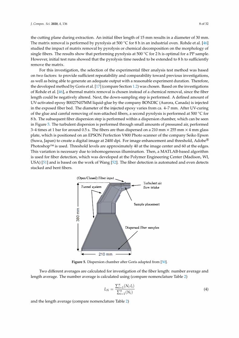
Table 4. µCT scan parameters GE v|tome|x m 240/180.

Parameter Unit Value

Voltage kV 80Current µA 140Voxel size µm 14.4Projections - 2000

The analysis of the µCT data is performed with VGSTUDIO MAX 3.3.0 64 Bit by the companyVolume graphics GmbH (Heidelberg, Germany). The software was chosen in accordance with acomparative study by Goris [17], which compared results of the conventional method of ellipsesto µCT-data analyzed with three different algorithms: VGSTUDIO MAX 3.3.0 64 Bit, slit method(SM) algorithm, and Mimics (proprietary to SABIC and Materialise MV). The results showed thata minimal resolution of 19 ± 1 µm could be used to sufficiently analyze the fiber orientation usingVGSTUDIO MAX. For this investigation, the analysis of isotropic fiber orientation is performed withplane projection. The direction of the normal vector is identical to the thickness direction. Table 5 showsthe detailed analysis parameters. As can be seen, the fiber material is defined by specific threshold,which is identical for all samples.

Table 5. Analysis parameters VGSTUDIO MAX 3.3.0 64 Bit.

Parameter Unit Value

Resolution µm 5Radius of integration µm 5Gradient threshold - 7Threshold for definition of the fiber material - 116Mode of integration for plane projection - isotrop

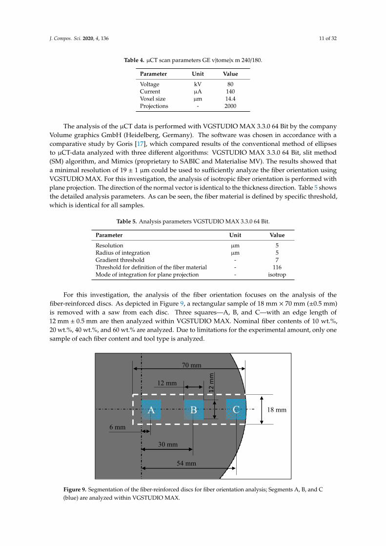
For this investigation, the analysis of the fiber orientation focuses on the analysis of thefiber-reinforced discs. As depicted in Figure 9, a rectangular sample of 18 mm × 70 mm (±0.5 mm)is removed with a saw from each disc. Three squares—A, B, and C—with an edge length of12 mm ± 0.5 mm are then analyzed within VGSTUDIO MAX. Nominal fiber contents of 10 wt.%,20 wt.%, 40 wt.%, and 60 wt.% are analyzed. Due to limitations for the experimental amount, only onesample of each fiber content and tool type is analyzed.

J. Compos. Sci. 2020, 4, x  11 of 32 

Table 4. μCT scan parameters GE v|tome|x m 240/180. 

Parameter  Unit  Value 

Voltage  kV  80 

Current  μA  140 

Voxel size  μm  14.4 

Projections  ‐  2000 

The analysis of the μCT data is performed with VGSTUDIO MAX 3.3.0 64 Bit by the company 

Volume graphics GmbH  (Heidelberg, Germany). The  software was  chosen  in  accordance with  a 

comparative study by Goris [17], which compared results of the conventional method of ellipses to 

μCT‐data analyzed with three different algorithms: VGSTUDIO MAX 3.3.0 64 Bit, slit method (SM) 

algorithm,  and Mimics  (proprietary  to  SABIC  and Materialise MV).  The  results  showed  that  a 

minimal  resolution  of  19±1  μm  could  be used  to  sufficiently  analyze  the  fiber  orientation using 

VGSTUDIO MAX. For this investigation, the analysis of isotropic fiber orientation is performed with 

plane projection. The direction of the normal vector  is  identical to the thickness direction. Table 5 

shows  the detailed  analysis parameters. As  can be  seen,  the  fiber material  is defined by  specific 

threshold, which is identical for all samples. 

Table 5. Analysis parameters VGSTUDIO MAX 3.3.0 64 Bit. 

Parameter  Unit  Value 

Resolution  μm  5 

Radius of integration  μm  5 

Gradient threshold  ‐  7 

Threshold for definition of the fiber material  ‐  116 

Mode of integration for plane projection  ‐  isotrop 

For this investigation, the analysis of the fiber orientation focuses on the analysis of the fiber‐

reinforced discs. As depicted  in Figure 9, a  rectangular  sample of 18 mm × 70 mm  (±0.5 mm)  is 

removed with a saw from each disc. Three squares—A, B, and C—with an edge length of 12 mm ± 

0.5 mm are then analyzed within VGSTUDIO MAX. Nominal fiber contents of 10 wt.%, 20 wt.%, 40 

wt.%, and 60 wt.% are analyzed. Due to limitations for the experimental amount, only one sample of 

each fiber content and tool type is analyzed. 

 

Figure 9. Segmentation of the fiber‐reinforced discs for fiber orientation analysis; Segments A, B, and 

C (blue) are analyzed within VGSTUDIO MAX. 

18 mm

70 mm

12 m

m

12 mm

6 mm

30 mm

54 mm

A CB

Figure 9. Segmentation of the fiber-reinforced discs for fiber orientation analysis; Segments A, B, and C(blue) are analyzed within VGSTUDIO MAX.

J. Compos. Sci. 2020, 4, 136 12 of 32

2.3. Processing Parameters and Tool Design

The processing parameters for STAMAX are based on the processing guidelines [53] recommendedby SABIC. Within these guidelines, a distinction is made between minimum, moderate, and maximumparameters. For this investigation, moderate parameters are targeted to generate comparability to theresults of Goris [50]. In accordance with the guidelines, the injection pressure is chosen at 800 barwith linear decline down to 700 bar for steel tooling, with moderate injection speeds of 70 ccm/s to60 ccm/s. The holding pressure is recommended at 50–80% of the injection pressure. Therefore, aholding pressure of 400 bar is chosen with a linear decline to 350 bar. Since aluminum and Bluestoneprovide lower mechanical properties than steel, the processing parameters including the clampingforce for these tools were lowered accordingly. Table 6 gives a detailed overview of the processingparameters of each tooling type.

Table 6. Processing parameters after [53].

Steel Aluminum Bluestone

Melt temperature in ◦C 250 250 250Mold temperature in ◦C 30 30 30Injection pressure in bar 800→ 700 500→ 400 400→ 250Injection speed in ccm/s 70→ 60 75→ 70 75→ 60Holding pressure in s 400→ 350 300→ 240 125→ 100Cooling time in s 65 65 85Clamping force in kN 220 180 170

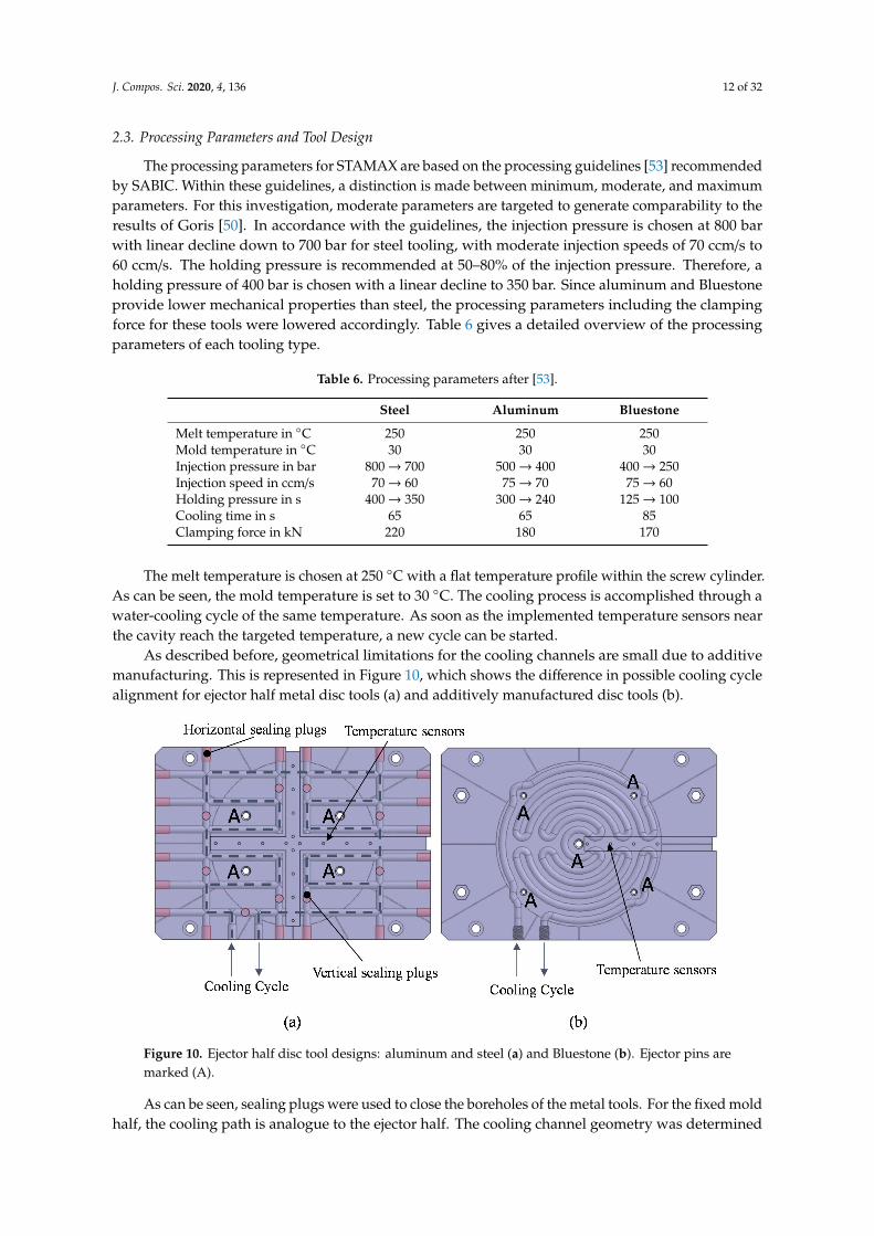
The melt temperature is chosen at 250 ◦C with a flat temperature profile within the screw cylinder.As can be seen, the mold temperature is set to 30 ◦C. The cooling process is accomplished through awater-cooling cycle of the same temperature. As soon as the implemented temperature sensors nearthe cavity reach the targeted temperature, a new cycle can be started.

As described before, geometrical limitations for the cooling channels are small due to additivemanufacturing. This is represented in Figure 10, which shows the difference in possible cooling cyclealignment for ejector half metal disc tools (a) and additively manufactured disc tools (b).

J. Compos. Sci. 2020, 4, x  12 of 32 

2.3. Processing Parameters and Tool Design 

The  processing  parameters  for  STAMAX  are  based  on  the  processing  guidelines  [53] 

recommended  by  SABIC.  Within  these  guidelines,  a  distinction  is  made  between  minimum, 

moderate, and maximum parameters. For  this  investigation, moderate parameters are  targeted  to 

generate comparability to the results of Goris [50]. In accordance with the guidelines, the injection 

pressure  is chosen at 800 bar with  linear decline down to 700 bar for steel tooling, with moderate 

injection speeds of 70 ccm/s  to 60 ccm/s. The holding pressure  is recommended at 50–80% of  the 

injection pressure. Therefore, a holding pressure of 400 bar is chosen with a linear decline to 350 bar. 

Since  aluminum  and  Bluestone  provide  lower mechanical  properties  than  steel,  the  processing 

parameters including the clamping force for these tools were lowered accordingly. Table 6 gives a 

detailed overview of the processing parameters of each tooling type. 

Table 6. Processing parameters after [53]. 

  Steel  Aluminum  Bluestone 

Melt temperature in °C  250  250  250 

Mold temperature in °C  30  30  30 

Injection pressure in bar  800  700  500  400  400  250 Injection speed in ccm/s  70  60  75  70  75  60 Holding pressure in s  400  350  300  240  125  100 Cooling time in s  65  65  85 

Clamping force in kN  220  180  170 

The melt  temperature  is  chosen  at  250  °C with  a  flat  temperature  profile within  the  screw 

cylinder. As can be seen, the mold temperature is set to 30 °C. The cooling process is accomplished 

through a water‐cooling cycle of  the same  temperature. As soon as  the  implemented  temperature 

sensors near the cavity reach the targeted temperature, a new cycle can be started. 

As described before, geometrical limitations for the cooling channels are small due to additive 

manufacturing. This is represented in Figure 10, which shows the difference in possible cooling cycle 

alignment for ejector half metal disc tools (a) and additively manufactured disc tools (b). 

 

Figure 10. Ejector half disc tool designs: aluminum and steel (a) and Bluestone (b). Ejector pins are 

marked (A). 

As can be seen, sealing plugs were used to close the boreholes of the metal tools. For the fixed 

mold  half,  the  cooling  path  is  analogue  to  the  ejector  half.  The  cooling  channel  geometry was 

determined through iterative calculation steps based on fundamental theorems of heat transfer and 

Figure 10. Ejector half disc tool designs: aluminum and steel (a) and Bluestone (b). Ejector pins aremarked (A).

As can be seen, sealing plugs were used to close the boreholes of the metal tools. For the fixed moldhalf, the cooling path is analogue to the ejector half. The cooling channel geometry was determined

J. Compos. Sci. 2020, 4, 136 13 of 32

through iterative calculation steps based on fundamental theorems of heat transfer and throughcalculation of the divergence in mold temperature. Moldflow simulations were used to guarantee ahomogenic average mold temperature of the developed concepts, to minimize the effect of differentcooling channel geometries on the results. As an example, the simulative results of Bluestone tensilespecimen-tools are depicted in Figure 11.

J. Compos. Sci. 2020, 4, x  13 of 32 

through  calculation  of  the divergence  in mold  temperature. Moldflow  simulations were used  to 

guarantee a homogenic average mold temperature of the developed concepts, to minimize the effect 

of  different  cooling  channel  geometries  on  the  results. As  an  example,  the  simulative  results  of 

Bluestone tensile specimen‐tools are depicted in Figure 11.   

 

Figure 11. Moldflow simulation results of the average temperature for tensile specimen‐tools out of 

Bluestone at 30 °C coolant temperature. 

As can be seen, the average temperature ranges from approximately 30 °C up to 125 °C. The 

highest  temperatures  can  be  seen  in  the  stagnation  points  of  the melt  at  the  tensile  specimen 

shoulders. Since for Bluestone, a uniform temperature could not be guaranteed within the whole part, 

the focus lied on creating a homogenous average temperature within the functional regions, which 

is the gauge for tensile specimens. The stagnation points (red) were defined as critical regions, which 

will be discussed further in the following chapter. In case of the tensile specimens, parabolic runners 

with a diameter of 5 mm and a non‐specified gate are used only on the ejector half. For the disc tools, 

the melt enters the cavity directly through the nozzle without the use of runners or a gate. The striking 

point of the melt also represents a critical region, especially for disc tools. 

3. Results 

3.1. Cycle Times Part Output and Failure‐Modes 

As can be seen in Figure 12, the recorded temperature near the critical region of tensile specimen 

Bluestone, aluminum, and steel tools are depicted. The final cycle times are determined through the 

critical mold  temperature of 30  °C. As soon as  the critical  temperature  is  reached, a new cycle  is 

started. 

 

 

Figure 12. Recorded temperatures near critical region of cavity within Bluestone, aluminum, and steel 

tools for tensile specimens. 

25

30

35

40

45

50

0 100 200 300 400 500 600 700 800

Tem

perature near critical region 

in °C

Time in s

Figure 11. Moldflow simulation results of the average temperature for tensile specimen-tools out ofBluestone at 30 ◦C coolant temperature.

As can be seen, the average temperature ranges from approximately 30 ◦C up to 125 ◦C. The highesttemperatures can be seen in the stagnation points of the melt at the tensile specimen shoulders. Sincefor Bluestone, a uniform temperature could not be guaranteed within the whole part, the focus liedon creating a homogenous average temperature within the functional regions, which is the gauge fortensile specimens. The stagnation points (red) were defined as critical regions, which will be discussedfurther in the following chapter. In case of the tensile specimens, parabolic runners with a diameter of5 mm and a non-specified gate are used only on the ejector half. For the disc tools, the melt enters thecavity directly through the nozzle without the use of runners or a gate. The striking point of the meltalso represents a critical region, especially for disc tools.

3. Results

3.1. Cycle Times Part Output and Failure-Modes

As can be seen in Figure 12, the recorded temperature near the critical region of tensile specimenBluestone, aluminum, and steel tools are depicted. The final cycle times are determined through thecritical mold temperature of 30 ◦C. As soon as the critical temperature is reached, a new cycle is started.

J. Compos. Sci. 2020, 4, x  13 of 32 

through  calculation  of  the divergence  in mold  temperature. Moldflow  simulations were used  to 

guarantee a homogenic average mold temperature of the developed concepts, to minimize the effect 

of  different  cooling  channel  geometries  on  the  results. As  an  example,  the  simulative  results  of 

Bluestone tensile specimen‐tools are depicted in Figure 11.   

 

Figure 11. Moldflow simulation results of the average temperature for tensile specimen‐tools out of 

Bluestone at 30 °C coolant temperature. 

As can be seen, the average temperature ranges from approximately 30 °C up to 125 °C. The 

highest  temperatures  can  be  seen  in  the  stagnation  points  of  the melt  at  the  tensile  specimen 

shoulders. Since for Bluestone, a uniform temperature could not be guaranteed within the whole part, 

the focus lied on creating a homogenous average temperature within the functional regions, which 

is the gauge for tensile specimens. The stagnation points (red) were defined as critical regions, which 

will be discussed further in the following chapter. In case of the tensile specimens, parabolic runners 

with a diameter of 5 mm and a non‐specified gate are used only on the ejector half. For the disc tools, 

the melt enters the cavity directly through the nozzle without the use of runners or a gate. The striking 

point of the melt also represents a critical region, especially for disc tools. 

3. Results 

3.1. Cycle Times Part Output and Failure‐Modes 

As can be seen in Figure 12, the recorded temperature near the critical region of tensile specimen 

Bluestone, aluminum, and steel tools are depicted. The final cycle times are determined through the 

critical mold  temperature of 30  °C. As soon as  the critical  temperature  is  reached, a new cycle  is 

started. 

 

 

Figure 12. Recorded temperatures near critical region of cavity within Bluestone, aluminum, and steel 

tools for tensile specimens. 

25

30

35

40

45

50

0 100 200 300 400 500 600 700 800

Tem

perature near critical region 

in °C

Time in s

Figure 12. Recorded temperatures near critical region of cavity within Bluestone, aluminum, and steeltools for tensile specimens.

J. Compos. Sci. 2020, 4, 136 14 of 32

As can be seen, through the immense thermal conductivity of aluminum tools, the temperature inthe depicted region fell even lower than 30 ◦C, close to room temperature, before a new cycle couldbe started. The results show that for every two Bluestone tool cycles, around seven steel cycles andeight aluminum cycles could be run. This directly translates to the increased thermal conductivityof steel and especially aluminum compared to Bluestone. In general, for every Bluestone tool typeover 100 parts could be manufactured for all represented nominal fiber contents which includes tooltrial runs. However, after a varying number of cycles depending on the tool type, different failuremodes could be detected which were assessed as discard criteria or could be temporarily overhauled.The most prominent failure modes and deteriorations are depicted in Figure 13.

J. Compos. Sci. 2020, 4, x  14 of 32 

As can be seen, through the immense thermal conductivity of aluminum tools, the temperature 

in the depicted region fell even lower than 30 °C, close to room temperature, before a new cycle could 

be started. The results show that for every two Bluestone tool cycles, around seven steel cycles and 

eight aluminum cycles could be run. This directly translates to the increased thermal conductivity of 

steel and especially aluminum compared to Bluestone. In general, for every Bluestone tool type over 

100 parts could be manufactured for all represented nominal fiber contents which includes tool trial 

runs. However, after a varying number of cycles depending on the tool type, different failure modes 

could be detected which were assessed as discard criteria or could be temporarily overhauled. The 

most prominent failure modes and deteriorations are depicted in Figure 13. 

 

Figure  13. Failure modes  and  tool deterioration during  specimen manufacturing: demolishing of 

mold at areas with strong staircase effect (a); clogging of channels at fiber contents of 60 wt.% (b); 

abrasion of mold material at the edges resulting  in flash on parts (c); penetration of mold through 

fibers and PP at regions of high impact (d); contamination of parts through scraped mold material (e). 

A typical challenge with additive manufactured components is the occurring staircase effect for 

steep geometries especially around angles of 45° paired with high temperatures. Figure 13 shows the 

critical regions with increased staircase effect (a), which caused demolishing of the mold especially 

at high fiber contents. For fiber contents of 60 wt.%, the demolishing eventually leads to clogging of 

channels at critical regions (Figure 13b). A typical deterioration for all nominal fiber contents is the 

abrasion of the mold material at the cavity edges (Figure 13c), which causes flashes on manufactured 

parts. This is either caused through underestimation of the clamping force, the flexibility of the mold 

or as an effect of repeated demolishing through material abrasion and heat exposure. A similar effect 

can be seen near the center of the mold and the melt entry point. After a non‐specified number of 

cycles,  these regions of high  impact showed penetration of  the mold  through  fibers and plain PP 

(Figure  13d).  In  extreme  cases,  the  scraped  mold  material  was  found  in  the  injected  molded 

components  (Figure 13e). Parts which  showed  signs of  foreign particles and  contamination were 

declared as rejects and the mold was eventually discarded. For aluminum and steel tools, none of the 

aforementioned failure modes or deteriorations could be detected. 

3.2. Mechanical Properties 

Generally, the results for the Young’s modulus (Figure 14) and the tensile strength (Figure 15) 

are increasing for rising nominal fiber contents, while the elongation at tensile strength (Figure 16) is 

Figure 13. Failure modes and tool deterioration during specimen manufacturing: demolishing of moldat areas with strong staircase effect (a); clogging of channels at fiber contents of 60 wt.% (b); abrasion ofmold material at the edges resulting in flash on parts (c); penetration of mold through fibers and PP atregions of high impact (d); contamination of parts through scraped mold material (e).

A typical challenge with additive manufactured components is the occurring staircase effect forsteep geometries especially around angles of 45◦ paired with high temperatures. Figure 13 shows thecritical regions with increased staircase effect (a), which caused demolishing of the mold especiallyat high fiber contents. For fiber contents of 60 wt.%, the demolishing eventually leads to clogging ofchannels at critical regions (Figure 13b). A typical deterioration for all nominal fiber contents is theabrasion of the mold material at the cavity edges (Figure 13c), which causes flashes on manufacturedparts. This is either caused through underestimation of the clamping force, the flexibility of the mold oras an effect of repeated demolishing through material abrasion and heat exposure. A similar effect canbe seen near the center of the mold and the melt entry point. After a non-specified number of cycles,these regions of high impact showed penetration of the mold through fibers and plain PP (Figure 13d).In extreme cases, the scraped mold material was found in the injected molded components (Figure 13e).Parts which showed signs of foreign particles and contamination were declared as rejects and the moldwas eventually discarded. For aluminum and steel tools, none of the aforementioned failure modes ordeteriorations could be detected.

3.2. Mechanical Properties

Generally, the results for the Young’s modulus (Figure 14) and the tensile strength (Figure 15)are increasing for rising nominal fiber contents, while the elongation at tensile strength (Figure 16) is

J. Compos. Sci. 2020, 4, 136 15 of 32

declining. Typical for brittle materials, the elongation at tensile strength and the elongation at breakare basically equal. The highest variation of the results is visible for nominal fiber contents of 60 wt.%.

  

J. Compos. Sci. 2020, 4, x; doi: FOR PEER REVIEW  www.mdpi.com/journal/jcs 

 

 Figure 14.: Young’s Modulus for tensile specimens from Bluestone™‐, Steel‐ and Aluminum‐ 

Tools for nominal fiber contents of 10, 20, 40 and 60 wt% 

2,000.00

4,000.00

6,000.00

8,000.00

10,000.00

12,000.00

14,000.00

10% 20% 40% 60%

Youngʹs M

odulus in M

Pa

Nominal Fiber Content

Figure 14. Young’s modulus for tensile specimens from Bluestone, steel, and aluminum tools fornominal fiber contents of 10 wt.%, 20 wt.%, 40 wt.%, and 60 wt.%.

J. Compos. Sci. 2020, 4, x  15 of 32 

declining. Typical for brittle materials, the elongation at tensile strength and the elongation at break 

are basically equal. The highest variation of the results is visible for nominal fiber contents of 60 wt.%. 

 

 

Figure 14. Young’s modulus  for  tensile  specimens  from Bluestone,  steel, and aluminum  tools  for 

nominal fiber contents of 10 wt.%, 20 wt.%, 40 wt.%, and 60 wt.%. 

The  results of  the Young’s modulus show  that comparable values  toward experimental data 

supported  by  the  manufacturer  are  reached  for  every  tool  type  and  nominal  fiber  content. 

Furthermore, Bluestone tool specimens of 60 wt.% nominal fiber content are showing slightly higher 

values  than  steel  and  aluminum  tools,  although  the  increased  variation  of  the  results must  be 

considered. An  almost  linear  increase  of  the  Young’s modulus  can  be  detected with  increasing 

nominal fiber contents, with maximum values around 12,000 MPa. 

 

 

Figure  15.  Tensile  strength  for  tensile  specimens  from  Bluestone,  steel,  and  aluminum  tools  for 

nominal fiber contents of 10 wt.%, 20 wt.%, 40 wt.%, and 60 wt.%. 

2000

4000

6000

8000

10000

12000

14000

10% 20% 40% 60%

Youngʹs M

odulus in M

Pa

Nominal Fiber Content

40

50

60

70

80

90

100

110

120

10% 20% 40% 60%

Tensile Strength in M

Pa

Nominal Fiber Content 

Figure 15. Tensile strength for tensile specimens from Bluestone, steel, and aluminum tools for nominalfiber contents of 10 wt.%, 20 wt.%, 40 wt.%, and 60 wt.%.

J. Compos. Sci. 2020, 4, 136 16 of 32

J. Compos. Sci. 2020, 4, x  16 of 32 

The  results  of  the  tensile  strength  also meet  nearly  identical  values  for  each  tool  type  and 

nominal  fiber  content. However,  there  is no detectable  increase  in  tensile  strength  from 40 wt.% 

toward  60 wt.%, with maximum  values  around  110 MPa  at  60 wt.%. As  described  before,  the 

deformation analysis is performed at higher testing speeds than the analysis of the elastic behavior. 

This must be considered for the comparison of the tensile strength as well as the elongation at tensile 

strength toward the manufacturers’ data. 

 

 

Figure 16. Elongation at tensile strength for tensile specimens from Bluestone, steel, and aluminum 

tools for nominal fiber contents of 10 wt.%, 20 wt.%, 40 wt.%, and 60 wt.%. 

The elongation at tensile strength shows a constant decline toward higher nominal fiber contents 

since the material gets increasingly brittle. Aluminum and steel tools show almost identical results. 

However,  test  specimens  of  Bluestone  tools  show  lower  values  than  aluminum  and  steel  tools, 

especially at nominal fiber contents of 40 wt.% and 60 wt.%. In further analysis, μCT data were able 

to show an increased number of voids for these nominal fiber contents, which are possibly caused 

due  to  limited  processing  conditions  (s.  Figure  17).  The  polymer  matrix  is  responsible  for  an 

improved elongation behavior since stresses in lateral direction can be minimized. Through voids, 

the elongation and elastic behaviors are locally reduced. 

 

Figure 17. μCT image from spattered voids in Bluestone tool specimens for a nominal fiber content 

and 60 wt.%. 

1,0

1,5

2,0

2,5

3,0

3,5

10% 20% 40% 60%

Elongation at Tensile Strength 

Nominal Fiber Content 

3.5

3.0

2.5

2.0

1.5

1.0

Figure 16. Elongation at tensile strength for tensile specimens from Bluestone, steel, and aluminumtools for nominal fiber contents of 10 wt.%, 20 wt.%, 40 wt.%, and 60 wt.%.

The results of the Young’s modulus show that comparable values toward experimental datasupported by the manufacturer are reached for every tool type and nominal fiber content. Furthermore,Bluestone tool specimens of 60 wt.% nominal fiber content are showing slightly higher values than steeland aluminum tools, although the increased variation of the results must be considered. An almostlinear increase of the Young’s modulus can be detected with increasing nominal fiber contents, withmaximum values around 12,000 MPa.

The results of the tensile strength also meet nearly identical values for each tool type and nominalfiber content. However, there is no detectable increase in tensile strength from 40 wt.% toward 60 wt.%,with maximum values around 110 MPa at 60 wt.%. As described before, the deformation analysis isperformed at higher testing speeds than the analysis of the elastic behavior. This must be consideredfor the comparison of the tensile strength as well as the elongation at tensile strength toward themanufacturers’ data.

The elongation at tensile strength shows a constant decline toward higher nominal fiber contentssince the material gets increasingly brittle. Aluminum and steel tools show almost identical results.However, test specimens of Bluestone tools show lower values than aluminum and steel tools, especiallyat nominal fiber contents of 40 wt.% and 60 wt.%. In further analysis, µCT data were able to show anincreased number of voids for these nominal fiber contents, which are possibly caused due to limitedprocessing conditions (Figure 17). The polymer matrix is responsible for an improved elongationbehavior since stresses in lateral direction can be minimized. Through voids, the elongation and elasticbehaviors are locally reduced.

J. Compos. Sci. 2020, 4, 136 17 of 32

J. Compos. Sci. 2020, 4, x  16 of 32 

The  results  of  the  tensile  strength  also meet  nearly  identical  values  for  each  tool  type  and 

nominal  fiber  content. However,  there  is no detectable  increase  in  tensile  strength  from 40 wt.% 

toward  60 wt.%, with maximum  values  around  110 MPa  at  60 wt.%. As  described  before,  the 

deformation analysis is performed at higher testing speeds than the analysis of the elastic behavior. 

This must be considered for the comparison of the tensile strength as well as the elongation at tensile 

strength toward the manufacturers’ data. 

 

 

Figure 16. Elongation at tensile strength for tensile specimens from Bluestone, steel, and aluminum 

tools for nominal fiber contents of 10 wt.%, 20 wt.%, 40 wt.%, and 60 wt.%. 

The elongation at tensile strength shows a constant decline toward higher nominal fiber contents 

since the material gets increasingly brittle. Aluminum and steel tools show almost identical results. 

However,  test  specimens  of  Bluestone  tools  show  lower  values  than  aluminum  and  steel  tools, 

especially at nominal fiber contents of 40 wt.% and 60 wt.%. In further analysis, μCT data were able 

to show an increased number of voids for these nominal fiber contents, which are possibly caused 

due  to  limited  processing  conditions  (s.  Figure  17).  The  polymer  matrix  is  responsible  for  an 

improved elongation behavior since stresses in lateral direction can be minimized. Through voids, 

the elongation and elastic behaviors are locally reduced. 

 

Figure 17. μCT image from spattered voids in Bluestone tool specimens for a nominal fiber content 

and 60 wt.%. 

1,0

1,5

2,0

2,5

3,0

3,5

10% 20% 40% 60%

Elongation at Tensile Strength 

Nominal Fiber Content 

3.5

3.0

2.5

2.0

1.5

1.0

Figure 17. µCT image from spattered voids in Bluestone tool specimens for a nominal fiber contentand 60 wt.%.

3.3. Fiber Length

The results of the fiber length analysis for a nominal fiber content of 40 wt.% are shown in Figure 18.All other results for 10 wt.%, 20 wt.%, and 60 wt.% are represented in Appendix A. Analogue to theresults of Goris [17] for steel tools, the length average of the fiber length reduces with increasingnominal fiber contents. The same phenomenon is visible for aluminum and Bluestone tools. Processingcauses severe fiber breakage, which causes the number of long fibers to reduce. With increasing fibercontents, the shear stress and fiber interlocking increases, which causes increased early state fiberbreakage. Therefore, the reached average values are far below the initial fiber length of 15 mm, withhigher values for the length average compared to the number average. The highest length averagevariations are visible close to the gate and the entry point of the melt (Location A). This is mostprominently visible for steel and aluminum tools at all nominal fiber contents. A possible explanationis the highly disoriented state in which the melt enters the cavity, thus creating a broader variety infiber length. This theory can be further supported by the length average values, which show highervarieties than number average values. As described before, the length average values tend to be morehighly impacted by the existence of a small number of relatively long fibers.

J. Compos. Sci. 2020, 4, x  17 of 32 

3.3. Fiber Length 

The results of the fiber length analysis for a nominal fiber content of 40 wt.% are shown in Figure 

18. All other results for 10 wt.%, 20 wt.%, and 60 wt.% are represented in Appendix A. Analogue to 

the results of Goris [17] for steel tools, the length average of the fiber length reduces with increasing 

nominal  fiber  contents.  The  same  phenomenon  is  visible  for  aluminum  and  Bluestone  tools. 

Processing causes severe  fiber breakage, which  causes  the number of  long  fibers  to  reduce. With 

increasing  fiber contents,  the shear stress and  fiber  interlocking  increases, which causes  increased 

early state fiber breakage. Therefore, the reached average values are far below the initial fiber length 

of 15 mm, with higher values for the length average compared to the number average. The highest 

length average variations are visible close to the gate and the entry point of the melt (Location A). 

This is most prominently visible for steel and aluminum tools at all nominal fiber contents. A possible 

explanation is the highly disoriented state in which the melt enters the cavity, thus creating a broader 

variety  in  fiber  length. This  theory can be  further supported by  the  length average values, which 

show higher varieties than number average values. As described before, the length average values 

tend to be more highly impacted by the existence of a small number of relatively long fibers. 

 

Figure 18. Fiber length (N = number average; W = weight or length average) for different tool types 

(for better representation in two diagrams) with 40 wt.% nominal fiber content at different specimen 

locations A, B, and C in accordance with Figure 7. 

Depending on the locations A, B, and C, the depicted fiber contents show different behaviors 

with an  increasing melt path. In general, the  length average values of each tool type show higher 

fluctuations over the melt path than the number average values, which show a nearly stable length 

around 0.6 mm  for all nominal  fiber contents and  tool  types. This value directly  translates  to  the 

results of Kim et al. [32], who declared a fiber length between 0.5–2 mm as typical values for long 

fibers after injection molding processing. Prominently stable results for the length average of each 

location are visible for Bluestone tools at nominal fiber contents of 40 wt.% and 60 wt.%, with a slight 

increase over the melt path (location A to C). Steel and aluminum tools show contrarian behaviors 

for nominal fiber contents of 40 wt.% and 60 wt.%, with maximum values at location A, followed by 

0

0,2

0,4

0,6

0,8

1

1,2

1,4

1,6

1,8

2

A B C

Fiber length in m

m

40 wt% Nominal Fiber Content 

0

0,2

0,4

0,6

0,8

1

1,2

1,4

1,6

1,8

2

A B C

Fiber length in m

m

40 wt% Nominal Fiber Content 

LN (Aluminum)

LW (Aluminum)

LN (Bluestone)

LW (Bluestone)

LN (Steel)

LW (Steel)

1.4

1.6

1.8

0.8

0.6

0.4

0.2

1

2

0

1.2

1.4

1.6

1.8

0.8

0.6

0.4

0.2

1

2

0

1.2

Figure 18. Fiber length (N = number average; W = weight or length average) for different tool types(for better representation in two diagrams) with 40 wt.% nominal fiber content at different specimenlocations A, B, and C in accordance with Figure 7.

J. Compos. Sci. 2020, 4, 136 18 of 32

Depending on the locations A, B, and C, the depicted fiber contents show different behaviorswith an increasing melt path. In general, the length average values of each tool type show higherfluctuations over the melt path than the number average values, which show a nearly stable lengtharound 0.6 mm for all nominal fiber contents and tool types. This value directly translates to the resultsof Kim et al. [32], who declared a fiber length between 0.5–2 mm as typical values for long fibers afterinjection molding processing. Prominently stable results for the length average of each location arevisible for Bluestone tools at nominal fiber contents of 40 wt.% and 60 wt.%, with a slight increase overthe melt path (location A to C). Steel and aluminum tools show contrarian behaviors for nominal fibercontents of 40 wt.% and 60 wt.%, with maximum values at location A, followed by a decrease overlocation B to C. For a nominal fiber content of 10 wt.%, the samples of Bluestone tools show a declinein length average from location A to B, while increasing to maximum values of around 1.8 mm inlocation C. This behavior is also present for steel and aluminum tools, although to a lesser extent andwith maximum values for the length average at location A. For 20 wt.% nominal fiber content, samplesof Bluestone tools show contrarian behavior compared to 10 wt.%, with high length average values atlocations A and B and a prominent decline in location C. A similar behavior is visible for aluminumtool samples, while samples from steel tools show almost identical behavior for 20 wt.% compared to10 wt.%.

Despite the discussed differences in length average for different tool types, the results showthat globally similar values for the average fiber length are reached depending of each tool material.Therefore, Bluestone tools can be declared viable for the use in functional validation of steel tools.

3.4. Fiber Concentration

The results of the fiber content analysis for a nominal fiber content of 40 wt.% are shown inFigure 19. All results for 10 wt.%, 20 wt.%, 40 wt.%, and 60 wt.% are represented in Figure 20.The schematic results for 10 wt.%, 20 wt.%, and 60 wt.% are shown in Appendix A. As can be seen,Figure 19 schematically depicts the results for an initial nominal fiber content of 40 wt.%, which showa characteristic increase in fiber content for all three tool types. This phenomenon can be seen for allinitial nominal fiber contents. The lowest fiber concentration can be seen around the disc center withvalues mostly below and around the initial nominal fiber concentration. With increasing flow path, thefiber content increases until reaching above average values within the disc edges. This general increaseof the fiber content with increasing melt path is visible for all nominal fiber contents, which is identicalto the results of Goris [50]. A possible hypothesis for this behavior is the increase of the shear stressbetween liquid melt and solidified regions. Two effects occur in these regions: fiber breakage andfiber pullout. Through shear forces in the border region, the fibers are carried away by the melt flowand are shortened in this process. In retrospective to the results of the fiber length in Section 3.3, thisphenomenon is especially visible on aluminum and steel tools. However, the results of Section 3.3 oftenshow a limited or contrarian fiber shortening behavior for Bluestone tools toward metal tools. This ispossibly caused by the slowed solidification and cooling process, as well as the limited processingconditions for Bluestone (injection speed, pressure, and clamping force). The fibers are more likely tobe pulled out and carried off, with limited fiber breakage due to a more gradually transition betweensolidified material and the flowing liquid melt.

J. Compos. Sci. 2020, 4, 136 19 of 32

J. Compos. Sci. 2020, 4, x  18 of 32 

a decrease over location B to C. For a nominal fiber content of 10 wt.%, the samples of Bluestone tools 

show a decline in length average from location A to B, while increasing to maximum values of around 

1.8 mm in location C. This behavior is also present for steel and aluminum tools, although to a lesser 

extent and with maximum values for the  length average at  location A. For 20 wt.% nominal fiber 

content, samples of Bluestone tools show contrarian behavior compared to 10 wt.%, with high length 

average values at  locations A and B and a prominent decline  in  location C. A similar behavior  is 

visible for aluminum tool samples, while samples from steel tools show almost identical behavior for 

20 wt.% compared to 10 wt.%. 

Despite the discussed differences in length average for different tool types, the results show that 

globally  similar values  for  the average  fiber  length are  reached depending of  each  tool material. 

Therefore, Bluestone tools can be declared viable for the use in functional validation of steel tools. 

3.4. Fiber Concentration 

The results of  the  fiber content analysis  for a nominal  fiber content of 40 wt.% are shown  in 

Figure 19. All results for 10 wt.%, 20 wt.%, 40 wt.%, and 60 wt.% are represented in Figure 20. The 

schematic results for 10 wt.%, 20 wt.%, and 60 wt.% are shown in Appendix A. As can be seen, Figure 

19 schematically depicts  the results  for an  initial nominal  fiber content of 40 wt.%, which show a 

characteristic increase in fiber content for all three tool types. This phenomenon can be seen for all 

initial nominal fiber contents. The lowest fiber concentration can be seen around the disc center with 

values mostly below and around the initial nominal fiber concentration. With increasing flow path, 

the fiber content increases until reaching above average values within the disc edges. This general 

increase of the fiber content with increasing melt path is visible for all nominal fiber contents, which 

is identical to the results of Goris [50]. A possible hypothesis for this behavior is the increase of the 

shear  stress between  liquid melt  and  solidified  regions. Two  effects occur  in  these  regions:  fiber 

breakage and fiber pullout. Through shear forces in the border region, the fibers are carried away by 

the melt flow and are shortened in this process. In retrospective to the results of the fiber length in 

chapter 3.3, this phenomenon is especially visible on aluminum and steel tools. However, the results 

of chapter 3.3 often show a limited or contrarian fiber shortening behavior for Bluestone tools toward 

metal tools. This is possibly caused by the slowed solidification and cooling process, as well as the 

limited processing conditions for Bluestone (injection speed, pressure, and clamping force). The fibers 

are more likely to be pulled out and carried off, with limited fiber breakage due to a more gradually 

transition between solidified material and the flowing liquid melt. 

 

Figure 19. Characteristic fiber content distribution pattern for disc segments of 40 wt.% initial nominal 

fiber content: steel  tool  (a), Bluestone  tool  (b), and aluminum  tool  (c). The color scheme describes 

values below (blue) up to values near (white) and values above (red) the initial nominal fiber content 

(in accordance with Figure 8). 

Figure 19. Characteristic fiber content distribution pattern for disc segments of 40 wt.% initial nominalfiber content: steel tool (a), Bluestone tool (b), and aluminum tool (c). The color scheme describesvalues below (blue) up to values near (white) and values above (red) the initial nominal fiber content(in accordance with Figure 8).

J. Compos. Sci. 2020, 4, x  19 of 32 

The  comparison  between  Bluestone  tools  and  steel  tools  for  all  initial  fiber  contents  is 

represented in Figure 20. For the comparison of steel and aluminum tools, see Appendix A. As can 

be seen, for an initial nominal fiber content of 10 wt.%, the overall values for Bluestone tool samples 

are below the values of steel tools. This can most likely be explained through inaccuracy in the before 

discussed gravimetric mixture of equal parts 20 wt.% fiber‐reinforced PP and plain PP. Regarding 

this, Bluestone tools and steel tools show nearly identical values and behaviors up to 40 wt.% initial 

nominal fiber content, with low standard variation. 60 wt.% samples from Bluestone tools show a 

higher spread toward minimum and maximum values compared to steel tools. This phenomenon is 

possibly caused by the gentler processing conditions for Bluestone tools. In comparison to the results 

of aluminum tools (see Appendix A), the results show that the best representation of steel tools for 

functional validation is through aluminum tools. However, the global fluctuation of the Bluestone 

tool samples is still low enough to be declared viable for functional validation of steel tools, especially 

for fiber contents up to 40 wt.%. The characteristic zones are identical for all tool types. 

 

 

Figure 20. Fiber content distribution  for disc segments of 10 wt.%, 20 wt.%, 40 wt.%, and 60 wt.% 

initial nominal fiber content at different locations (1–33 in accordance with Figure 7) for steel tools 

and Bluestone tools. 

0

10

20

30

40

50

60

70

1 3 5 7 9 11 13 15 17 19 21 23 25 27 29 31 33

Fiber content in w

t%

Sample Location

Figure 20. Fiber content distribution for disc segments of 10 wt.%, 20 wt.%, 40 wt.%, and 60 wt.%initial nominal fiber content at different locations (1–33 in accordance with Figure 7) for steel tools andBluestone tools.

J. Compos. Sci. 2020, 4, 136 20 of 32

The comparison between Bluestone tools and steel tools for all initial fiber contents is representedin Figure 20. For the comparison of steel and aluminum tools, see Appendix A. As can be seen, for aninitial nominal fiber content of 10 wt.%, the overall values for Bluestone tool samples are below thevalues of steel tools. This can most likely be explained through inaccuracy in the before discussedgravimetric mixture of equal parts 20 wt.% fiber-reinforced PP and plain PP. Regarding this, Bluestonetools and steel tools show nearly identical values and behaviors up to 40 wt.% initial nominal fibercontent, with low standard variation. 60 wt.% samples from Bluestone tools show a higher spreadtoward minimum and maximum values compared to steel tools. This phenomenon is possibly causedby the gentler processing conditions for Bluestone tools. In comparison to the results of aluminum tools(see Appendix A), the results show that the best representation of steel tools for functional validation isthrough aluminum tools. However, the global fluctuation of the Bluestone tool samples is still lowenough to be declared viable for functional validation of steel tools, especially for fiber contents up to40 wt.%. The characteristic zones are identical for all tool types.

3.5. Fiber Orientation

As described in Section 1.2, seven characteristic regions can be determined in injection moldedparts. Figure 21 shows the orientation tensor components over the relative sample thickness exemplifiedfor a nominal fiber content of 60 wt.% at location B of a Bluestone tool specimen segment (in accordancewith Figure 9). As can be seen, the characteristic zones can be identified (1, 2 and 3).

J. Compos. Sci. 2020, 4, x  20 of 32 

3.5. Fiber Orientation 

As described in chapter 1.2, seven characteristic regions can be determined in injection molded 

parts.  Figure  21  shows  the  orientation  tensor  components  over  the  relative  sample  thickness 

exemplified for a nominal fiber content of 60 wt.% at location B of a Bluestone tool specimen segment 

(in accordance with Figure 9). As can be seen, the characteristic zones can be identified (1, 2 and 3).   

 

Figure 21. Orientation tensor components (𝑎 , 𝑎 , 𝑎 ) over relative sample thickness for a nominal 

fiber  content of 60 wt.%  (Bluestone  tool;  segment B), with  characteristic zones after Osswald and 

Menges [36] (shell layers = 1, core layer = 2, transition layers/skin layers = 3). 

In addition to the identification of the characteristic zones, it is visible that the tensor component 

𝑎   is constant over the entire relative sample thickness. This is valid for all examined segments. For 

further analysis of the fiber orientation, only components  𝑎 and  𝑎   are described because of their 

relevance  toward  the  identification  of  the  characteristic  zones. Figure  22  shows  the  results  for  a 

nominal fiber content of 60 wt.% for Bluestone tools, steel tools and aluminum tools at locations A, 

B, and C. The results of all other nominal fiber contents can be seen in Appendix A. 

Figure 21. Orientation tensor components (a11, a22, a33) over relative sample thickness for a nominalfiber content of 60 wt.% (Bluestone tool; segment B), with characteristic zones after Osswald andMenges [36] (shell layers = 1, core layer = 2, transition layers/skin layers = 3).

J. Compos. Sci. 2020, 4, 136 21 of 32

In addition to the identification of the characteristic zones, it is visible that the tensor componenta33 is constant over the entire relative sample thickness. This is valid for all examined segments.For further analysis of the fiber orientation, only components a11 and a22 are described because oftheir relevance toward the identification of the characteristic zones. Figure 22 shows the results for anominal fiber content of 60 wt.% for Bluestone tools, steel tools and aluminum tools at locations A, B,and C. The results of all other nominal fiber contents can be seen in Appendix A.

J. Compos. Sci. 2020, 4, x 21 of 32

Figure 22. Orientation tensor components (𝑎𝑎11 , 𝑎𝑎22 ; without 𝑎𝑎33for better overview) and relative sample thickness fora nominal fiber content of 60 wt.%. Specimens were created with Bluestone, steel, and aluminum tools, with samples from regions A, B, and C (in accordance with Figure 9).

As can be seen, the quality of the results is highly dependent on the sample location. Since B provides the most developed, unhindered, and oriented state of the melt flow, the characteristic zones are identifiable without further complication. Location A provides the most inconsistent transitions compared to locations B and C. A possible explanation for this behavior can be given based on the melt flow state. Since the melt flow is in a highly disoriented state when it enters the cavity, it is most likely that this region shows the highest inconsistencies toward fiber orientation. This behavior is present for all tool types and nominal fiber contents. Location C shows more consistent results than location A. However, due to the material stagnation at the edges of the disc, slight inconsistencies that hinder clear identification of the characteristic zones are still visible. Therefore, the decision was made to concentrate on location B entirely for the identification of specific trends dependent on increasing nominal fiber content, as well as different tool materials. The results can be seen in Figure 23.

0 0,2 0,4 0,6 0,8 1

Ori

enta

tion

Tens

or C

ompo

nent

s aij

Relative Sample Thickness

B A

C

a11 a22

0

0,2

0,4

0,6

0,8

1

0 0,2 0,4 0,6 0,8 1

Aluminium C0

0,2

0,4

0,6

0,8

1

Aluminium B

Aluminium A

0

0,2

0,4

0,6

0,8

1

0 0,2 0,4 0,6 0,8 1

BS C0

0,2

0,4

0,6

0,8

1

0 0,2 0,4 0,6 0,8 1

BS B0

0,2

0,4

0,6

0,8

1

0 0,2 0,4 0,6 0,8 1

BS A

0 0,2 0,4 0,6 0,8 1

Aluminum

0 0,2 0,4 0,6 0,8 1

SteelBluestone

60 % Nominal Fiber Content

Figure 22. Orientation tensor components (a11, a22; without a33 for better overview) and relative samplethickness fora nominal fiber content of 60 wt.%. Specimens were created with Bluestone, steel, andaluminum tools, with samples from regions A, B, and C (in accordance with Figure 9).

As can be seen, the quality of the results is highly dependent on the sample location. Since Bprovides the most developed, unhindered, and oriented state of the melt flow, the characteristic zonesare identifiable without further complication. Location A provides the most inconsistent transitionscompared to locations B and C. A possible explanation for this behavior can be given based on themelt flow state. Since the melt flow is in a highly disoriented state when it enters the cavity, it is mostlikely that this region shows the highest inconsistencies toward fiber orientation. This behavior ispresent for all tool types and nominal fiber contents. Location C shows more consistent results than

J. Compos. Sci. 2020, 4, 136 22 of 32

location A. However, due to the material stagnation at the edges of the disc, slight inconsistencies thathinder clear identification of the characteristic zones are still visible. Therefore, the decision was madeto concentrate on location B entirely for the identification of specific trends dependent on increasingnominal fiber content, as well as different tool materials. The results can be seen in Figure 23.J. Compos. Sci. 2020, 4, x 22 of 32

Figure 23. Orientation tensor components (𝑎𝑎11 , 𝑎𝑎22 ; without 𝑎𝑎33for better overview) and relative sample thickness for nominal fiber contents of 10 wt.%, 20 wt.%, 40 wt.%, and 60 wt.%. Specimens were created with Bluestone, steel, and aluminum tools.

It can be seen that there is a global increase of the shell layer thickness with increasing nominal fiber contents. A possible hypothesis for this phenomenon is based on different crystallization behavior for increasing fiber contents. Each fiber in the melt acts as a nucleating agent during cooldown. When more fibers are included, the crystallization process and solidification take place faster, which benefits increasing shell thickness. In terms of applicability for functional validation of steel tools, the Bluestone tools show almost identical fiber orientation compared to steel and aluminum tools. The thickness of the specific zones and the range of the orientation tensors are almost identical for all used tool types, which is essential for the qualification of Bluestone tools for functional validation. However, further repeated experiments are necessary for a sufficient qualification, since only one specimen of each tool type and nominal fiber content was examined

Ori

enta

tion

Tens

or C

ompo

nent

s a i

j

Relative Sample Thickness

10 %

20

%40

%

a11 a22

60 %

0

0,2

0,4

0,6

0,8

1

0 0,2 0,4 0,6 0,8 1

Aluminium B

0

0,2

0,4

0,6

0,8

1

0 0,2 0,4 0,6 0,8 1

BS B

0 0,2 0,4 0,6 0,8 1

Stahl B 0

0,2

0,4

0,6

0,8

1

0 0,2 0,4 0,6 0,8 1

Aluminium B

0

0,2

0,4

0,6

0,8

1

0 0,2 0,4 0,6 0,8 1

BS B

0 0,2 0,4 0,6 0,8 1

Stahl B 0

0,2

0,4

0,6

0,8

1

0 0,2 0,4 0,6 0,8 1

Aluminium B

0

0,2

0,4

0,6

0,8

1

0 0,2 0,4 0,6 0,8 1

BS B

0 0,2 0,4 0,6 0,8 1

Stahl B 0

0,2

0,4

0,6

0,8

1

0 0,2 0,4 0,6 0,8 1

Aluminium B

0

0,2

0,4

0,6

0,8

1

0 0,2 0,4 0,6 0,8 1

Bluestone B SteelBluestone Aluminium

B B B

B B B

B B B

B B B

Figure 23. Orientation tensor components (a11, a22; without a33 for better overview) and relative samplethickness for nominal fiber contents of 10 wt.%, 20 wt.%, 40 wt.%, and 60 wt.%. Specimens were createdwith Bluestone, steel, and aluminum tools.

It can be seen that there is a global increase of the shell layer thickness with increasing nominalfiber contents. A possible hypothesis for this phenomenon is based on different crystallization behaviorfor increasing fiber contents. Each fiber in the melt acts as a nucleating agent during cooldown. When

J. Compos. Sci. 2020, 4, 136 23 of 32

more fibers are included, the crystallization process and solidification take place faster, which benefitsincreasing shell thickness. In terms of applicability for functional validation of steel tools, the Bluestonetools show almost identical fiber orientation compared to steel and aluminum tools. The thickness ofthe specific zones and the range of the orientation tensors are almost identical for all used tool types,which is essential for the qualification of Bluestone tools for functional validation. However, furtherrepeated experiments are necessary for a sufficient qualification, since only one specimen of each tooltype and nominal fiber content was examined during the experiments. Furthermore, the differentthermal conductivities of all tool types impact the viscosity of the melt, which must be analyzed tosolidify the aforementioned hypothesis.

4. Discussion & Conclusions

The discussion of the results of this investigation concentrates on two different aspects:

(a) The general identification of characteristic phenomena dependent on the type of tool materialand the nominal fiber content.

(b) The relevance of the results toward the overall target, to use additively manufactured Bluestonetools as an alternative for steel tools for spare part and small series productions, as well as for thefunctional validation of steel tools.

The results of this investigation successfully illustrate, that specimens manufactured withBluestone tools show comparable results toward metal tools for the mechanical properties and thefiber configuration, which includes fiber length, fiber concentration, and fiber orientation. In termsof the cycle times, the part output and the tool durability, Bluestone tools are not able compete withmetal tools. As expected, zones of high impact and choke points proof to be critical for the Bluestonetool durability. A possible solution would be the use of modular concepts that make use of overallusable metal inlets, which can be applied at highly stressed regions. However, for the use of Bluestonetools in spare part and small series production, the reached part output of over 100 parts proves tobe sufficient. Due to the similarity in fiber configuration and the mechanical properties, the use ofBluestone tools for functional validation is nearly qualified. Further experiments toward the fiberorientation need to be conducted to solidify the existing results.

Multiple characteristic phenomena could be detected, which are applicable for polymer tools,aluminum tools, and steel tools. For all tool types, the extent of the nominal fiber content influencestwo aspects: the thickness of the characteristic zones defined by Osswald and Menges [36], as wellas the fiber length average. The analysis of the fiber orientation shows that with increasing nominalfiber content, the thickness of the shell layers increases respectively, while the thickness of the corelayer decreases. A possible hypothesis for this phenomenon is based on the altered crystallizationmechanism for increasing fiber contents. When more fibers are included, the crystallization processand solidification take place faster, which benefits increasing shell thickness. The analysis of the fiberlength illustrates that the length average for specimens of each tool material decreases with increasingnominal fiber contents. The number average stays nearly stable for all tool types around 0.6 mm.This value directly translates to the results of Kim et al. [32], which declared a fiber length between0.5–2 mm as typical values for long fibers after injection molding processing. Another phenomenon isdetermined through the analysis of the fiber concentration. Analogous to the results for rectangularspecimens created through steel tools described by Goris [50], a gradual decrease of the fiber content isvisible with increasing melt flow distance. This behavior is visible for steel tool specimens and now forBluestone tool and aluminum tool specimens as well. A characteristic maximum at the edges of thedisc specimens can be declared.

All in all, additively manufactured Bluestone proofs to be a viable approach for the rapid creationof polymer tools for injection molding processing. Further investigations will be centered around theimprovement of the polymer tool lifecycle, as well as improved cycle times through efficient coolingmethods. The use of modular concepts that make use of overall usable metal inlets needs to be further

J. Compos. Sci. 2020, 4, 136 24 of 32

investigated. At last, the cost efficiency of polymer tools toward metal tools needs to be analyzed for aspecific example in a comparative study.

Author Contributions: This investigation is based in equal parts on the scientific work of L.K. and R.S., underthe supervision of D.R., K.W. and T.O. The work was divided in the following categories: Conceptualization,L.K.; methodology, L.K. and R.S.; software, L.K. and R.S.; validation, L.K. and R.S.; formal analysis, L.K. andR.S.; investigation, L.K. and R.S.; data curation, L.K. and R.S.; writing—original draft preparation, L.K. and R.S.;writing—review and editing, L.K. and R.S.; visualization, L.K. and R.S.; supervision, D.R., K.W., T.O.; projectadministration, L.K.; funding acquisition, no additional/external funding. All authors have read and agreed to thepublished version of the manuscript.

Funding: This research received no external funding. The APC was funded by Polymer Engineering Center,University of Wisconsin-Madison, Madison, WI 53706, USA.

Conflicts of Interest: The authors declare there is no conflict of interest.

Appendix A

J. Compos. Sci. 2020, 4, x 24 of 32

Prof. T.O.; project administration, L.K.; funding acquisition, no additional/external funding. All authors have read and agreed to the published version of the manuscript.

Funding: This research received no external funding. The APC was funded by Polymer Engineering Center, University of Wisconsin-Madison, Madison, WI 53706, USA.

Conflicts of Interest: The authors declare there is no conflict of interest.

Appendix A

Figure A1. Orientation tensor components (𝑎𝑎11, 𝑎𝑎22; without 𝑎𝑎33for better overview) and relative sample thickness for a nominal fiber content of 10 wt.%. Specimens were created with Bluestone, steel, and aluminum tools, with samples from regions A, B, and C (in accordance with Figure 9).

0

0,2

0,4

0,6

0,8

1

0 0,2 0,4 0,6 0,8 1

Aluminium C0

0,2

0,4

0,6

0,8

1

Aluminium B

Aluminium A

0

0,2

0,4

0,6

0,8

1

0 0,2 0,4 0,6 0,8 1

Bluestone C0

0,2

0,4

0,6

0,8

1

0 0,2 0,4 0,6 0,8 1

Bluestone B0

0,2

0,4

0,6

0,8

1

0 0,2 0,4 0,6 0,8 1

Bluestone A

0 0,2 0,4 0,6 0,8 1

Stahl C0 0,2 0,4 0,6 0,8 1

Stahl B0 0,2 0,4 0,6 0,8 1

Stahl A

Ori

enta

tion

Tens

or C

ompo

nent

s aij

Relative Sample Thickness

Bluestone™ Steel Aluminum

B A

C

a11 a22

10 % Nominal Fiber Content

Figure A1. Orientation tensor components (a11, a22; without a33 for better overview) and relativesample thickness for a nominal fiber content of 10 wt.%. Specimens were created with Bluestone, steel,and aluminum tools, with samples from regions A, B, and C (in accordance with Figure 9).

J. Compos. Sci. 2020, 4, 136 25 of 32J. Compos. Sci. 2020, 4, x 25 of 32

Figure A2. Orientation tensor components (𝑎𝑎11, 𝑎𝑎22; without 𝑎𝑎33for better overview) and relative sample thickness for a nominal fiber content of 20 wt.%. Specimens were created with Bluestone, steel, and aluminum tools, with samples from regions A, B, and C (in accordance with Figure 9).

Ori

enta

tion

Tens

or C

ompo

nent

s aij

Relative Sample Thickness

B A

C

a11 a22

0

0,2

0,4

0,6

0,8

1

0 0,2 0,4 0,6 0,8 1

Aluminium C0

0,2

0,4

0,6

0,8

1

0

0,2

0,4

0,6

0,8

1

0 0,2 0,4 0,6 0,8 1

BS C0

0,2

0,4

0,6

0,8

1

0 0,2 0,4 0,6 0,8 1

BS B0

0,2

0,4

0,6

0,8

1

0 0,2 0,4 0,6 0,8 1

BS A

0 0,2 0,4 0,6 0,8 1

Stahl C0 0,2 0,4 0,6 0,8 1

Stahl B0 0,2 0,4 0,6 0,8 1

Stahl ABluestone™ Steel Aluminum

20 % Nominal Fiber Content

Figure A2. Orientation tensor components (a11, a22; without a33 for better overview) and relativesample thickness for a nominal fiber content of 20 wt.%. Specimens were created with Bluestone, steel,and aluminum tools, with samples from regions A, B, and C (in accordance with Figure 9).

J. Compos. Sci. 2020, 4, 136 26 of 32J. Compos. Sci. 2020, 4, x 26 of 32

Figure A3. Orientation tensor components (𝑎𝑎11, 𝑎𝑎22; without 𝑎𝑎33for better overview) and relative sample thickness for a nominal fiber content of 40 wt.%. Specimens were created with Bluestone, steel, and aluminum tools, with samples from regions A, B, and C (in accordance with Figure 9).

0

0,2

0,4

0,6

0,8

1

0 0,2 0,4 0,6 0,8 1

Ori

enta

tion

Tens

or C

ompo

nent

s aij

Relative Sample Thickness

A

BC

a11 a22

0

0,2

0,4

0,6

0,8

1

0 0,2 0,4 0,6 0,8 1

Aluminium C0

0,2

0,4

0,6

0,8

1

Aluminium B

0

0,2

0,4

0,6

0,8

1

0 0,2 0,4 0,6 0,8 1

0

0,2

0,4

0,6

0,8

1

0 0,2 0,4 0,6 0,8 1

0 0,2 0,4 0,6 0,8 1

Stahl C

SteelBluestone™

40 % Nominal Fiber Content

Aluminum

Figure A3. Orientation tensor components (a11, a22; without a33 for better overview) and relativesample thickness for a nominal fiber content of 40 wt.%. Specimens were created with Bluestone, steel,and aluminum tools, with samples from regions A, B, and C (in accordance with Figure 9).

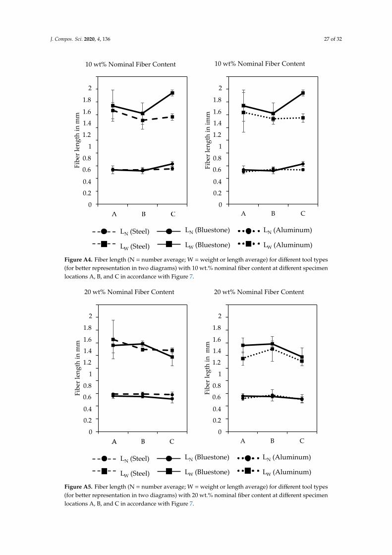
J. Compos. Sci. 2020, 4, 136 27 of 32J. Compos. Sci. 2020, 4, x 27 of 32

Figure A4. Fiber length (N = number average; W = weight or length average) for different tool types (for better representation in two diagrams) with 10 wt.% nominal fiber content at different specimen locations A, B, and C in accordance with Figure 7.

Figure A5. Fiber length (N = number average; W = weight or length average) for different tool types (for better representation in two diagrams) with 20 wt.% nominal fiber content at different specimen locations A, B, and C in accordance with Figure 7.

0

0,2

0,4

0,6

0,8

1

1,2

1,4

1,6

1,8

2

1 2 3

Fibe

r len

gth

in m

m

10 wt% Nominal Fiber Content

0

0,2

0,4

0,6

0,8

1

1,2

1,4

1,6

1,8

2

A B CFi

ber l

engt

h in

imm

10 wt% Nominal Fiber Content

LN (Aluminum)

LW (Aluminum)

LN (Bluestone)

LW (Bluestone)

LN (Steel)

LW (Steel)

1.4

1.6

1.8

0.8

0.6

0.4

0.2

1

2

0

1.2

1.4

1.6

1.8

0.8

0.6

0.4

0.2

1

2

0

1.2

0

0,2

0,4

0,6

0,8

1

1,2

1,4

1,6

1,8

2

1 2 3

Fibe

r len

gth

in m

m

20 wt% Nominal Fiber Content

0

0,2

0,4

0,6

0,8

1

1,2

1,4

1,6

1,8

2

A B C

Fibe

r leg

th in

mm

20 wt% Nominal Fiber Content

LN (Aluminum)

LW (Aluminum)

LN (Bluestone)

LW (Bluestone)

LN (Steel)

LW (Steel)

1.4

1.6

1.8

0.8

0.6

0.4

0.2

1

2

0

1.2

1.4

1.6

1.8

0.8

0.6

0.4

0.2

1

2

0

1.2

Figure A4. Fiber length (N = number average; W = weight or length average) for different tool types(for better representation in two diagrams) with 10 wt.% nominal fiber content at different specimenlocations A, B, and C in accordance with Figure 7.

J. Compos. Sci. 2020, 4, x 27 of 32

Figure A4. Fiber length (N = number average; W = weight or length average) for different tool types (for better representation in two diagrams) with 10 wt.% nominal fiber content at different specimen locations A, B, and C in accordance with Figure 7.

Figure A5. Fiber length (N = number average; W = weight or length average) for different tool types (for better representation in two diagrams) with 20 wt.% nominal fiber content at different specimen locations A, B, and C in accordance with Figure 7.

0

0,2

0,4

0,6

0,8

1

1,2

1,4

1,6

1,8

2

1 2 3

Fibe

r len

gth

in m

m

10 wt% Nominal Fiber Content

0

0,2

0,4

0,6

0,8

1

1,2

1,4

1,6

1,8

2

A B CFi

ber l

engt

h in

imm

10 wt% Nominal Fiber Content

LN (Aluminum)

LW (Aluminum)

LN (Bluestone)

LW (Bluestone)

LN (Steel)

LW (Steel)

1.4

1.6

1.8

0.8

0.6

0.4

0.2

1

2

0

1.2

1.4

1.6

1.8

0.8

0.6

0.4

0.2

1

2

0

1.2

0

0,2

0,4

0,6

0,8

1

1,2

1,4

1,6

1,8

2

1 2 3

Fibe

r len

gth

in m

m

20 wt% Nominal Fiber Content

0

0,2

0,4

0,6

0,8

1

1,2

1,4

1,6

1,8

2

A B C

Fibe

r leg

th in

mm

20 wt% Nominal Fiber Content

LN (Aluminum)

LW (Aluminum)

LN (Bluestone)

LW (Bluestone)

LN (Steel)

LW (Steel)

1.4

1.6

1.8

0.8

0.6

0.4

0.2

1

2

0

1.2

1.4

1.6

1.8

0.8

0.6

0.4

0.2

1

2

0

1.2

Figure A5. Fiber length (N = number average; W = weight or length average) for different tool types(for better representation in two diagrams) with 20 wt.% nominal fiber content at different specimenlocations A, B, and C in accordance with Figure 7.

J. Compos. Sci. 2020, 4, 136 28 of 32J. Compos. Sci. 2020, 4, x 28 of 32

Figure A6. Fiber length (N = number average; W = weight or length average) for different tool types (for better representation in two diagrams) with 60 wt.% nominal fiber content at different specimen locations A, B, and C in accordance with Figure 7.

Figure A7. Characteristic fiber content distribution pattern for disc segments of 10 wt.%, 20 wt.%, and 60 wt.% initial nominal fiber content: steel tool (a), Bluestone tool (b), and aluminum tool (c). The

0

0,2

0,4

0,6

0,8

1

1,2

1,4

1,6

1,8

2

1 2 3

Fibe

r len

gth

in m

m

60 wt% Nominal Fiber Content

0

0,2

0,4

0,6

0,8

1

1,2

1,4

1,6

1,8

2

A B C

Fibe

r len

gth

in m

m

60 wt% Nominal Fiber Content

LN (Aluminum)

LW (Aluminum)

LN (Bluestone)

LW (Bluestone)

LN (Steel)

LW (Steel)

1.4

1.6

1.8

0.8

0.6

0.4

0.2

1

2

0

1.2

1.4

1.6

1.8

0.8

0.6

0.4

0.2

1

2

0

1.2

10 wt%

BluestoneSteel

20 wt%

60 wt%

Aluminum(a) (b) (c)

Figure A6. Fiber length (N = number average; W = weight or length average) for different tool types(for better representation in two diagrams) with 60 wt.% nominal fiber content at different specimenlocations A, B, and C in accordance with Figure 7.

J. Compos. Sci. 2020, 4, x  28 of 32 

 

Figure A6. Fiber length (N = number average; W = weight or length average) for different tool types 

(for better representation in two diagrams) with 60 wt.% nominal fiber content at different specimen 

locations A, B, and C in accordance with Figure 7. 

 

Figure A7. Characteristic fiber content distribution pattern for disc segments of 10 wt.%, 20 wt.%, and 

60 wt.%  initial nominal  fiber content: steel  tool  (a), Bluestone  tool  (b), and aluminum  tool  (c). The 

20,51 20,46 20,68 20,76

20,37 20,29 20,51 20,48 19,99

20,09 19,80 20,45 20,38 20,89 19,94

19,49 19,87 20,24 20,18 20,67 20,33

19,23 19,74 20,43 19,99 20,29 20,48

19,21 19,40 20,19 20,16 20,05 20,45

10,54 10,36 10,67 10,71

11,13 11,60 11,68 11,28 11,58

10,86 11,27 11,37 11,17 11,31 10,90

10,76 10,96 11,11 10,99 11,08 11,25

10,14 10,83 10,35 10,65 10,97 11,11

10,71 10,96 10,76 10,63 11,18 10,98

61,09 61,37 61,55 60,12

59,40 59,79 60,81 61,85 61,12

57,99 58,05 58,47 59,76 61,51 61,08

58,30 57,83 58,24 59,09 60,43 61,37

58,78 58,34 57,86 58,23 59,49 61,35

59,12 59,30 57,98 58,38 58,97 61,02

63,95 64,59 65,29 64,54

56,19 57,33 60,60 65,18 65,25

55,59 55,63 56,87 57,69 64,67 65,55

56,89 56,59 56,18 56,38 60,51 65,79

59,15 59,02 57,48 56,52 57,60 65,48

59,19 59,50 57,60 56,56 57,43 64,94

20,12 19,99 19,84 20,02

19,64 19,93 19,90 19,94 19,53

19,38 19,55 19,46 19,64 19,95 19,63

19,44 19,28 19,42 19,61 19,88 20,01

18,28 18,82 19,14 19,57 19,80 20,09

18,18 18,09 18,72 19,08 19,87 20,13

8,04 8,35 8,09 7,92

8,18 8,36 8,58 8,63 8,32

8,12 8,27 8,84 8,96 8,77 8,38

7,82 8,39 8,60 8,61 8,76 8,22

7,25 8,09 8,27 8,29 8,43 8,08

7,36 7,82 8,22 8,64 8,67 8,35

10 wt%

BluestoneSteel

20 wt%

60 wt%

11,39 11,40 10,89 9,72

11,66 11,71 11,58 11,85 11,02

11,01 11,06 11,34 12,05 11,55 10,72

10,28 10,43 10,71 11,71 12,00 11,19

9,95 10,10 10,62 10,89 11,66 11,49

10,21 9,94 10,46 10,80 11,70 11,63

Aluminum

20,33 20,29 20,54 20,27

19,69 19,82 19,99 20,27 20,64

19,36 19,75 19,67 19,96 20,41 20,62

18,72 19,14 19,74 19,97 20,06 20,52

18,32 18,69 19,41 19,87 20,05 20,32

18,65 18,81 19,24 19,79 19,92 20,21

60,70 60,65 60,43 59,70

59,17 59,37 60,05 60,78 59,95

58,18 58,42 58,90 59,91 61,02 60,66

58,56 58,25 58,49 59,54 60,54 61,14

59,06 59,19 58,58 58,82 59,90 61,38

58,62 58,46 58,41 58,45 59,87 61,31

(a) (b) (c)

Figure A7. Characteristic fiber content distribution pattern for disc segments of 10 wt.%, 20 wt.%, and60 wt.% initial nominal fiber content: steel tool (a), Bluestone tool (b), and aluminum tool (c). The colorscheme describes values below (blue) up to values near (white) and values above (red) the initialnominal fiber content (in accordance with Figure 8).

J. Compos. Sci. 2020, 4, 136 29 of 32

J. Compos. Sci. 2020, 4, x  29 of 32 

color scheme describes values below (blue) up to values near (white) and values above (red) the initial 

nominal fiber content (in accordance with Figure 8). 

 

 

Figure A8. Fiber content distribution for disc segments of 10, 20, 40, and 60 wt.% initial nominal fiber 

content at different locations (1–33 in accordance with Figure 7) for steel tools and aluminum tools. 

References 

1. Schemme, M. LFT—Development status and perspectives. Reinf. Plast. 2008, 52, 32–39 2. Henning,  F.;  Ernst,  H.;  Brüssel,  R.  LFTs  for  automotive  applications.  Reinf.  Plast.  2005,  49,  24–33, 

doi:10.1016/s0034‐3617(05)00546‐1. 

3. Markets and Markets Research Private Ltd. Long Fiber Thermoplastics Market by Resin (PP, PA, PEEK, PPA), 

Fiber  (Glass,  Carbon),  Manufacturing  Process  (Injection  Molding,  Pultrusion,  D‐LFT),  End‐Use  Industry 

(Automotive, Electrical & Electronics), Region‐Global Forecast to 2025; Markets and Markets Research Private 

Ltd.: Magarpatta, India, 2020.   

4. Markarian, J. Long fibre reinforcement drives automotive market forward. Plast. Addit. Compd. 2005, 7, 24–

29, doi:10.1016/s1464‐391x(05)70393‐7. 

0

10

20

30

40

50

60

70

1 3 5 7 9 11 13 15 17 19 21 23 25 27 29 31 33

Fibe

r C

onte

nt [

%w

t]

Sample Location [-]

Figure A8. Fiber content distribution for disc segments of 10, 20, 40, and 60 wt.% initial nominal fibercontent at different locations (1–33 in accordance with Figure 7) for steel tools and aluminum tools.

References

1. Schemme, M. LFT—Development status and perspectives. Reinf. Plast. 2008, 52, 32–39. [CrossRef]2. Henning, F.; Ernst, H.; Brüssel, R. LFTs for automotive applications. Reinf. Plast. 2005, 49, 24–33. [CrossRef]3. Markets and Markets Research Private Ltd. Long Fiber Thermoplastics Market by Resin (PP, PA, PEEK, PPA),

Fiber (Glass, Carbon), Manufacturing Process (Injection Molding, Pultrusion, D-LFT), End-Use Industry (Automotive,Electrical & Electronics), Region-Global Forecast to 2025; Markets and Markets Research Private Ltd.: Magarpatta,India, 2020.

4. Markarian, J. Long fibre reinforcement drives automotive market forward. Plast. Addit. Compd. 2005, 7,24–29. [CrossRef]

5. Gómez-Monterde, J.; Sánchez-Soto, M.; Maspoch, M.L. Microcellular PP/GF composites: Morphological,mechanical and fracture characterization. Compos. Part A Appl. Sci. Manuf. 2018, 104, 1–13. [CrossRef]

J. Compos. Sci. 2020, 4, 136 30 of 32

6. SmartTech Analysis. Additive Manufacturing Market Outlook and Summary of Opportunities; SmartTech Analysis:Charlottesville, VA, USA, 2019.

7. Ngo, T.; Kashani, A.; Imbalzano, G.; Nguyen, Q.; Hui, D. Additive manufacturing (3D printing): A review ofmaterials, methods, applications and challenges. Compos. Part B Eng. 2018, 143, 172–196. [CrossRef]

8. Shaffer, S.; Yang, K.; Vargas, J.; Di Prima, M.; Voit, W. On reducing anisotropy in 3D printed polymers viaionizing radiation. Polymer 2014, 55, 5969–5979. [CrossRef]

9. Zou, R.; Xia, Y.; Liu, S.; Hu, P.; Hou, W.; Hu, Q.; Shan, C. Isotropic and anisotropic elasticity and yielding of3D printed material. Compos. Part B Eng. 2016, 99, 506–513. [CrossRef]

10. Valino, A.D.; Dizon, J.R.C.; Espera, A.H., Jr.; Chen, Q.; Messman, J.; Advincula, R.C. Advances in 3D printingof thermoplastic polymer composites and nanocomposites. Prog. Polym. Sci. 2019, 98, 101162. [CrossRef]

11. Achillas, C.; Tzetzis, D.; Raimondo, M.O. Alternative production strategies based on the comparison ofadditive and traditional manufacturing technologies. Int. J. Prod. Res. 2017, 55, 1–13. [CrossRef]

12. Rohde, J.; Jahnke, U.; Lindemann, C.; Kruse, A.; Koch, R. Standardised product development for technologyintegration of additive manufacturing. Virtual Phys. Prototyp. 2018, 14, 141–147. [CrossRef]

13. Wu, T.; Jahan, S.A.; Kumaar, P.; Tovar, A.; El-Mounayri, H.; Zhang, Y.; Zhang, J.; Acheson, D.; Brand, K.;Nalim, R. A framework for optimizing the design of injection molds with conformal cooling for additivemanufacturing. Procedia Manuf. 2015, 1, 404–415. [CrossRef]

14. Maravola, M.; Conner, B.; Walker, J.; Cortes, P. Epoxy infiltrated 3D printed ceramics for composite toolingapplications. Addit. Manuf. 2019, 25, 59–63. [CrossRef]

15. Yuan, S.; Shen, F.; Chua, C.K.; Zhou, K. Polymeric composites for powder-based additive manufacturing:Materials and applications. Prog. Polym. Sci. 2019, 91, 141–168. [CrossRef]

16. Kampker, A.; Triebs, J.; Kawollek, S.; Ayvaz, P.; Beyer, T. Direct polymer additive tooling—Effect of additivemanufactured polymer tools on part material properties for injection moulding. Rapid Prototyp. J. 2019.[CrossRef]

17. Goris, S.; Back, T.; Yanev, A.; Brands, D.; Drummer, D.; Osswald, T.A. A novel fiber length measurementtechnique for discontinuous fiber-reinforced composites: A comparative study with existing methods. Polym.Compos. 2017, 39, 4058–4070. [CrossRef]

18. Sodeifian, G.; Ghaseminejad, S.; Yousefi, A.A. Preparation of polypropylene/short glass fiber composite asFused Deposition Modeling (FDM) filament. Results Phys. 2019, 12, 205–222. [CrossRef]

19. Hertle, S.; Drexler, M.; Drummer, D. Additive manufacturing of poly(propylene) by means of melt extrusion.Macromol. Mater. Eng. 2016, 301, 1482–1493. [CrossRef]

20. Mulholland, T.; Goris, S.; Boxleitner, J.; Osswald, T.; Rudolph, N. Process-induced fiber orientation in fusedfilament fabrication. J. Compos. Sci. 2018, 2, 45. [CrossRef]

21. Kampker, A.; Triebs, J.; Ford, B.A.; Kawollek, S.; Ayvaz, P. Potential analysis of additive manufacturingtechnologies for fabrication of polymer tools for injection moulding—A comparative study. In Proceedingsof the 2018 IEEE International Conference on Advanced Manufacturing, Yunlin, Taiwan, 16–18 November2018.

22. Rahmati, S.; Dickens, P. Rapid tooling analysis of stereolithography injection mould tooling. Int. J. Mach.Tools Manuf. 2007, 47, 740–747. [CrossRef]

23. Summer Topical Meeting; American Society for Precision Engineering; European Society for PrecisionEngineering; Nanotechnology. Dimensional accuracy and surface finish in additive manufacturing.In Proceedings of the ASPE—The American Society for Precision Engineering, Raleigh, NC, USA,27–30 June 2016.

24. Altaf, K.; Rani, A.M.A.; Raghavan, V.R. Prototype production and experimental analysis for circular andprofiled conformal cooling channels in aluminium filled epoxy injection mould tools. Rapid Prototyp. J. 2013,19, 220–229. [CrossRef]

25. Park, H.S.; Dang, X.-P. Development of a smart plastic injection mold with conformal cooling channels.Procedia Manuf. 2017, 10, 48–59. [CrossRef]

26. Hopkinson, N.; Dickens, P. A comparison between stereolithography and aluminium injection mouldingtooling. Rapid Prototyp. J. 2000, 6, 253–258. [CrossRef]

27. Martinho, P.G.; Bartolo, P.J.; Pouzada, A. Hybrid moulds: Effect of the moulding blocks on the morphologyand dimensional properties. Rapid Prototyp. J. 2009, 15, 71–82. [CrossRef]

J. Compos. Sci. 2020, 4, 136 31 of 32

28. Harris, R.; Fouchal, F.; Hague, R.; Dickens, P. Quantifying part irregularities and subsequent morphologymanipulation in stereolithography plastic injection moulding. Plast. Rubber Compos. 2004, 33, 92–98.[CrossRef]

29. Harris, R.A.; Hague, R.J.; Dickens, P.M. Crystallinity control in parts produced from stereolithographyinjection mould tooling. Proc. Inst. Mech. Eng. Part L J. Mater. Des. Appl. 2003, 217, 269–276. [CrossRef]

30. Fernandes, A.D.C.; De Souza, A.F.; Howarth, J.L.L. Mechanical and dimensional characterisation ofpolypropylene injection moulded parts in epoxy resin/aluminium inserts for rapid tooling. Int. J. Mater.Prod. Technol. 2016, 52, 37. [CrossRef]

31. Volpato, N.; Solis, D.M.; Costa, C.A. An analysis of digital ABS as a rapid tooling material for polymerinjection moulding. Int. J. Mater. Prod. Technol. 2016, 52. [CrossRef]

32. Kim, Y.; Park, O.O. Effect of fiber length on mechanical properties of injection molded long-fiber-reinforcedthermoplastics. Macromol. Res. 2020, 28, 1–12. [CrossRef]

33. Seong, D.G.; Kang, C.; Pak, S.Y.; Kim, C.H.; Song, Y.S. Influence of fiber length and its distribution in threephase poly(propylene) composites. Compos. Part B Eng. 2019, 168, 218–225. [CrossRef]

34. Hou, X.; Chen, X.; Liu, B.; Chen, S.; Li, H.; Cao, W. Fracture and orientation of long-glass-fiber-reinforcedpolypropylene during injection molding. Polym. Eng. Sci. 2020, 60, 13–21. [CrossRef]

35. Tadmor, Z. Molecular orientation in injection molding. J. Appl. Polym. Sci. 1974, 18, 1753–1772. [CrossRef]36. Osswald, T.A. Understanding Polymer Processing: Processes and Governing Equations; Hanser Publications:

Munich, Germany, 2017.37. Parveeen, B.; Caton-Rose, P.; Costa, F.; Jin, X.; Hine, P. Study of injection moulded long glass fibre-reinforced

polypropylene and the effect on the fibre length and orientation distribution. AIP Conf. Proc. 2014, 1593,432–435.

38. Zhu, H.; Gu, Y.; Yang, Z.; Li, Q.; Li, M.; Wang, S.; Zhang, Z. Fiber distribution of long fiber reinforcedpolyamide and effect of fiber orientation on mechanical behavior. Polym. Compos. 2020, 41, 1531–1550.[CrossRef]

39. Lafranche, E.; Krawczak, P. Injection moulding of long glass fibre reinforced thermoplastics (LFT):Structure/processing conditions/mechanical properties relationship. In Proceedings of the ESAFORMConference on Material Forming, Glasgow, UK, 26–28 April 2006.

40. Kunc, V.; Frame, B.J.; Nguyen, B.N.; Tucker, C.L., III; Velez-Garcia, G. Fiber length distribution measurementfor long glass and carbon fiber reinforced injection molded thermoplastics. Res. Gate 2007, Volume 2, 866–876.

41. Ren, P.; Dai, G. Fiber dispersion and breakage in deep screw channel during processing of long fiber-reinforcedpolypropylene. Fibers Polym. 2014, 15, 1507–1516. [CrossRef]

42. Krasteva, D.L. Integrated Prediction of Processing and Thermomechanical Behavior of Long FiberThermoplastic Composites. Ph.D. Thesis, University of Minho, Braga, Portugal, 2009.

43. Sharma, B.N.; Naragani, D.; Nguyen, B.N.; Tucker, C.L.; Sangid, M.D. Uncertainty quantification of fiberorientation distribution measurements for long-fiber-reinforced thermoplastic composites. J. Compos. Mater.2018, 52, 1781–1797. [CrossRef]

44. Advani, S.G. The use of tensors to describe and predict fiber orientation in short fiber composites. J. Rheol.1987, 31, 751–784. [CrossRef]

45. Chen, H.; Baird, D.G. Prediction of young’s modulus for injection molded long fiber reinforced thermoplastics.J. Compos. Sci. 2018, 2, 47. [CrossRef]

46. Rohde, M.; Ebel, A.; Wolff-Fabris, F.; Altstädt, V. Influence of processing parameters on the fiber length andimpact properties of injection molded long glass fiber reinforced polypropylene. Int. Polym. Process. 2011,26, 292–303. [CrossRef]

47. 3D Systems. Accura Bluestone Technical Data Sheet 2018. Available online: https://de.3dsystems.com/

sites/default/files/2018-08/3d-systems-accura-bluestone-datasheet-uken-2018-08-21-web.pdf (accessed on7 August 2020).

48. Wilzer, J.; Lüdtke, F.; Weber, S.; Theisen, W. The influence of heat treatment and resulting microstructures onthe thermophysical properties of martensitic steels. J. Mater. Sci. 2013, 48, 8483–8492. [CrossRef]

49. Ostermann, F. Anwendungstechnologie Aluminium; Springer Science and Business Media LLC: Berlin,Germany, 1998.

50. Goris, S. Characterization of the Process-Induced Fiber Configuration of Long Glass Fiber-ReinforcedThermoplastics. Ph.D. Dissertation, University of Wisconsin, Madison, WI, USA, 2017.

J. Compos. Sci. 2020, 4, 136 32 of 32

51. Perez, C.; Osswald, T.A.; Goris, S. Study on the fiber properties of a LFT strand. SPE ACCE 2013, 2, 1115–1126.52. Wang, H. Fiber Property Characterization by Image Processing. Master’s Thesis, Texas Tech University,

Lubbock, TX, USA, 2007.53. SABIC. Processing Guides: SABIC Stamax; SABIC: Riyadh, Saudi Arabia, 2016.

© 2020 by the authors. Licensee MDPI, Basel, Switzerland. This article is an open accessarticle distributed under the terms and conditions of the Creative Commons Attribution(CC BY) license (http://creativecommons.org/licenses/by/4.0/).