COMP 150-AVS

Fall 2018

Data Flow Analysis

2

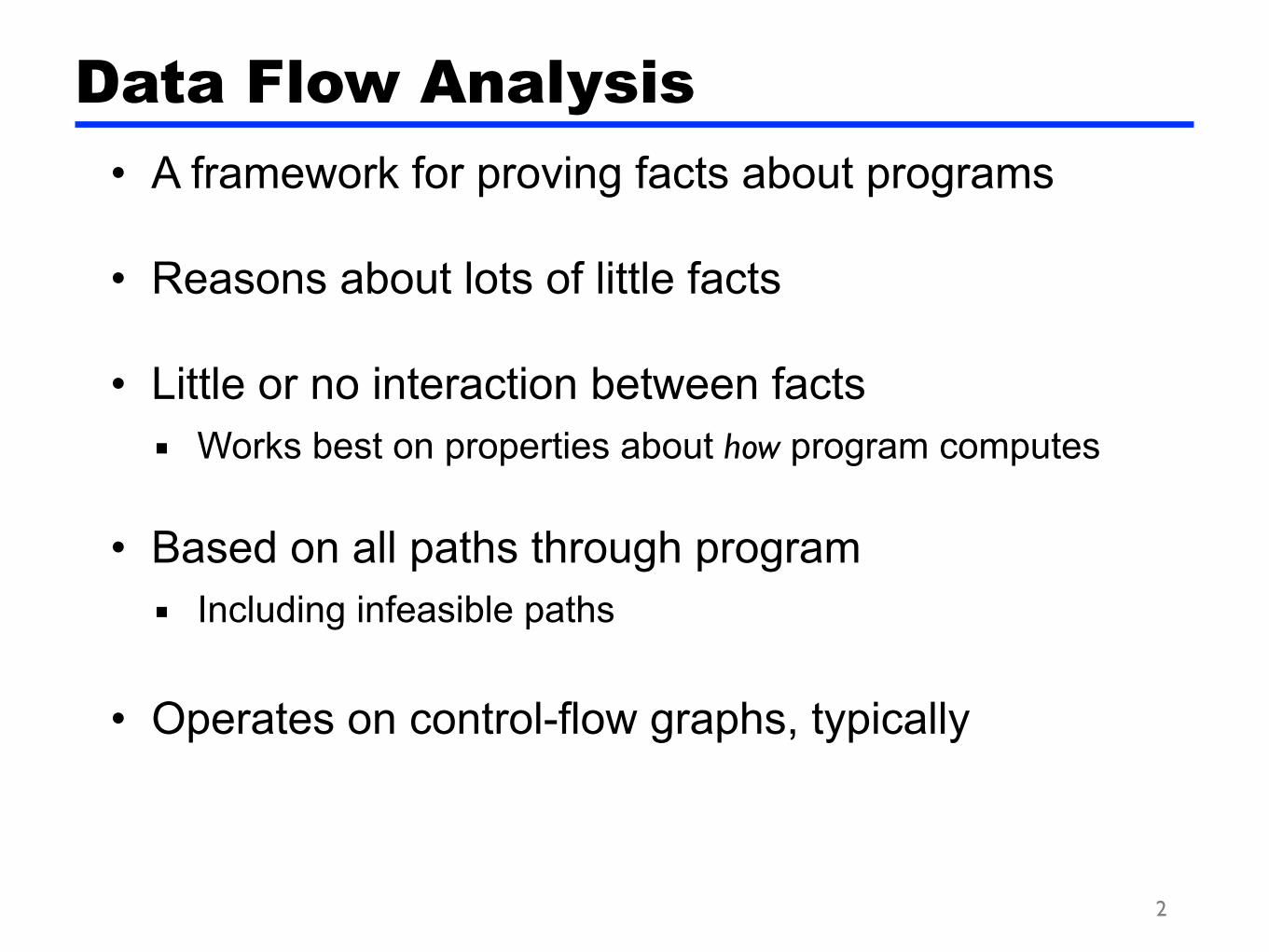
• A framework for proving facts about programs

• Reasons about lots of little facts

• Little or no interaction between facts ■ Works best on properties about how program computes

• Based on all paths through program ■ Including infeasible paths

• Operates on control-flow graphs, typically

Data Flow Analysis

3

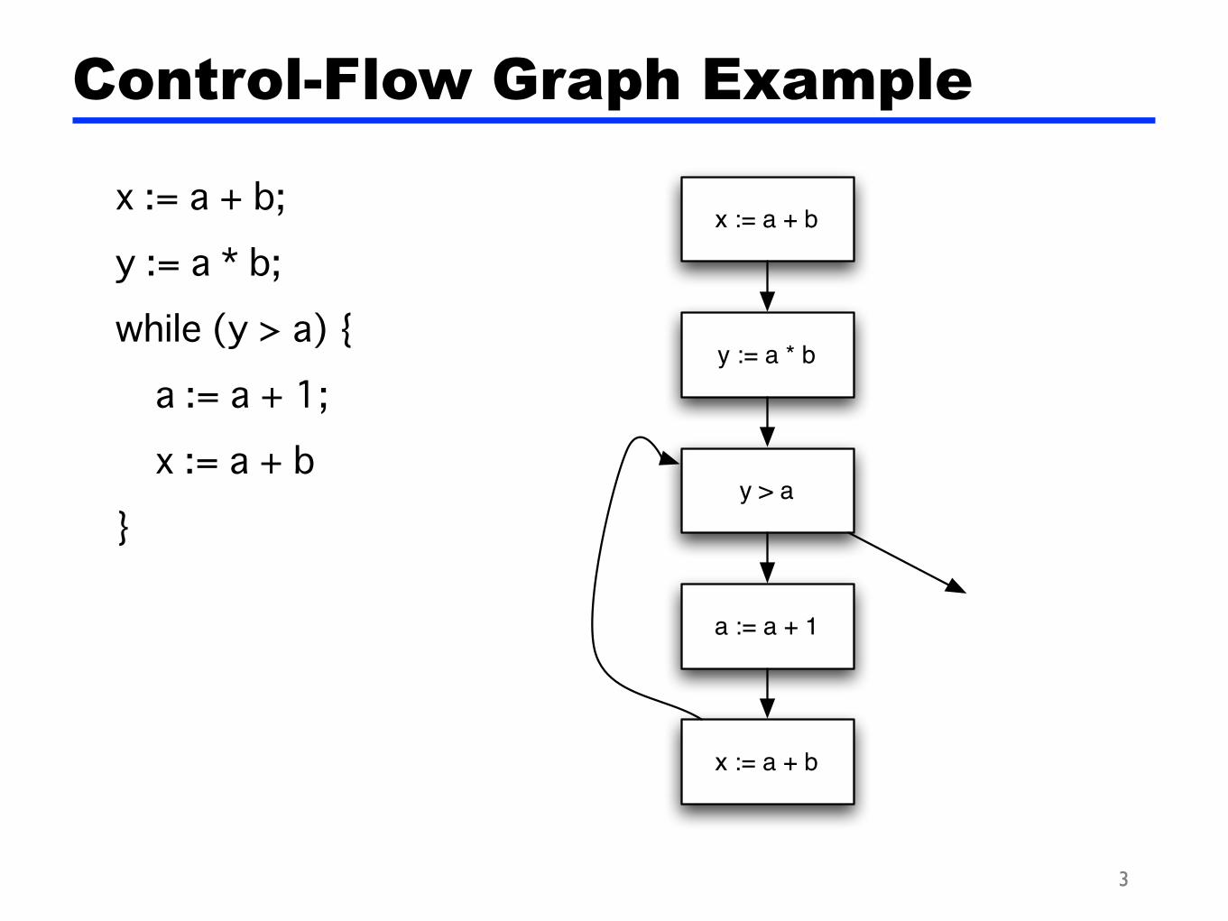
x := a + b;

y := a * b;

while (y > a) {

a := a + 1;

x := a + b

}

Control-Flow Graph Example

x := a + b

y := a * b

y > a

a := a + 1

x := a + b

4

Control-Flow Graph w/Basic Blocks

• Can lead to more efficient implementations • But more complicated to explain, so...

■ We’ll use single-statement blocks in lecture today

x := a + b; y := a * b; while (y > a + b) { a := a + 1; x := a + b }

x := a + by := a * b

y > a

a := a + 1x := a + b

5

x := a + b;

y := a * b;

while (y > a) {

a := a + 1;

x := a + b

}

• All nodes without a (normal) predecessor should be pointed to by entry

•All nodes without a successor should point to exit

Example with Entry and Exit

x := a + b

y := a * b

y > a

a := a + 1

x := a + b

exit

entry

Notes on Entry and Exit

• Typically, we perform data flow analysis on a function body

• Functions usually have ■ A unique entry point ■ Multiple exit points

• So in practice, there can be multiple exit nodes in the CFG ■ For the rest of these slides, we’ll assume there’s only one ■ In practice, just treat all exit nodes the same way as if

there’s only one exit node

6

7

• An expression e is available at program point p if ■ e is computed on every path to p, and ■ the value of e has not changed since the last time e was

computed on the paths to p

• Optimization ■ If an expression is available, need not be recomputed

- (At least, if it’s still in a register somewhere)

Available Expressions

8

• Is expression e available? • Facts:

■ a + b is available ■ a * b is available ■ a + 1 is available

Data Flow Facts

x := a + b

y := a * b

y > a

a := a + 1

x := a + b

exit

entry

9

• What is the effect of each statement on the set of facts?

Gen and Kill

Stmt Gen Kill

x := a + b a + b

y := a * b a * b

a := a + 1a + 1,a + b,a * b

x := a + b

y := a * b

y > a

a := a + 1

x := a + b

exit

entry

10

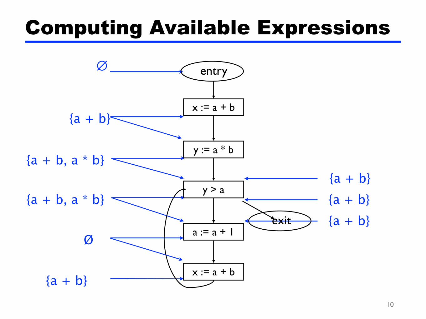
Computing Available Expressions

∅

{a + b}

{a + b, a * b}

{a + b, a * b}

Ø

{a + b}

{a + b}{a + b}{a + b}

x := a + b

y := a * b

y > a

a := a + 1

x := a + b

entry

exit

11

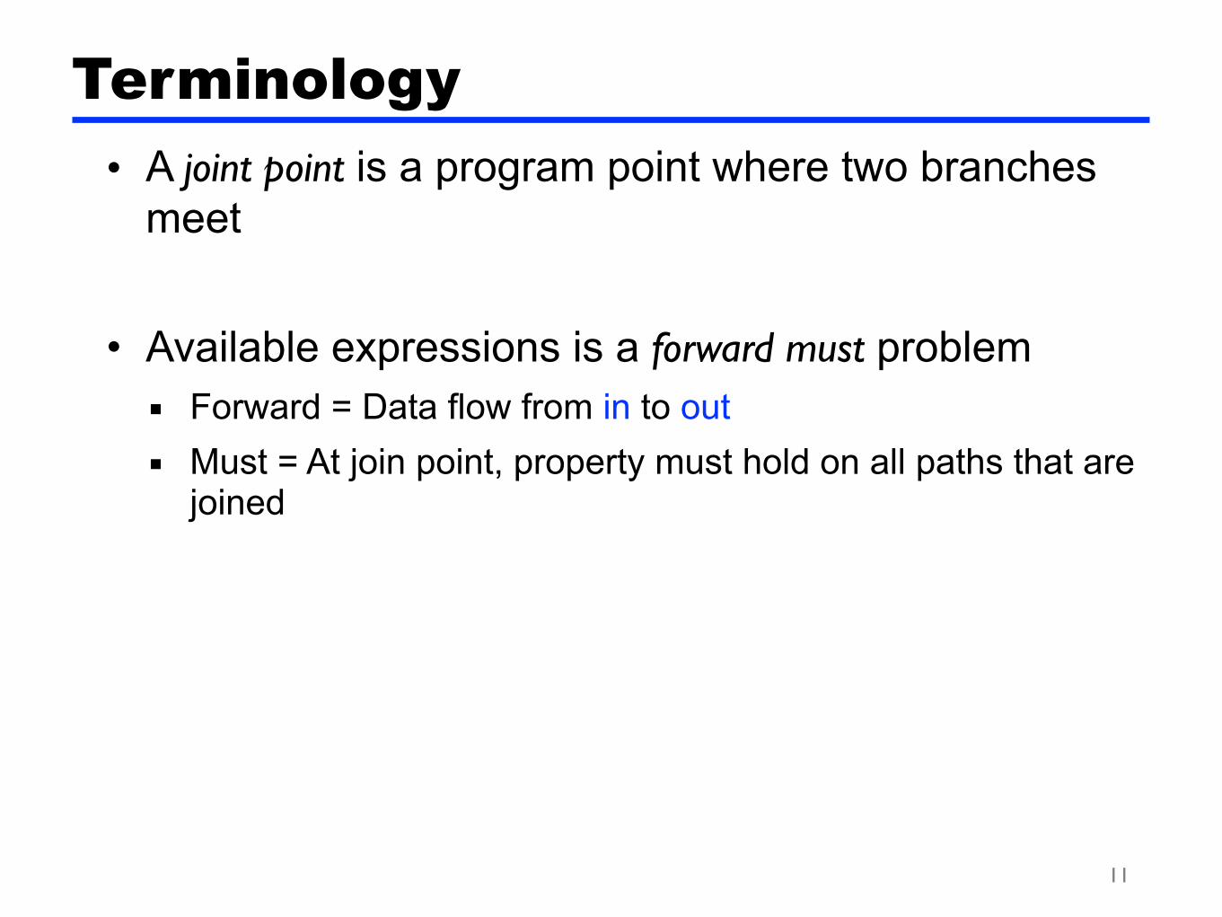
Terminology

• A joint point is a program point where two branches meet

• Available expressions is a forward must problem ■ Forward = Data flow from in to out ■ Must = At join point, property must hold on all paths that are

joined

12

• Let s be a statement ■ succ(s) = { immediate successor statements of s } ■ pred(s) = { immediate predecessor statements of s} ■ in(s) = program point just before executing s ■ out(s) = program point just after executing s

• in(s) = ∩s′ ∊ pred(s) out(s′)

• out(s) = gen(s) ∪ (in(s) - kill(s))

■ Note: These are also called transfer functions

Data Flow Equations

13

• A variable v is live at program point p if ■ v will be used on some execution path originating from p... ■ before v is overwritten

• Optimization ■ If a variable is not live, no need to keep it in a register ■ If variable is dead at assignment, can eliminate assignment

Liveness Analysis

14

• Available expressions is a forward must analysis ■ Data flow propagate in same dir as CFG edges ■ Expr is available only if available on all paths

• Liveness is a backward may problem ■ To know if variable live, need to look at future uses ■ Variable is live if used on some path

• out(s) = ∪s′ ∊ succ(s) in(s′)

• in(s) = gen(s) ∪ (out(s) - kill(s))

Data Flow Equations

15

• What is the effect of each statement on the set of facts?

Gen and Kill

Stmt Gen Kill

x := a + b a, b x

y := a * b a, b y

y > a a, y

a := a + 1 a a

x := a + b

y := a * b

y > a

a := a + 1

x := a + b

16

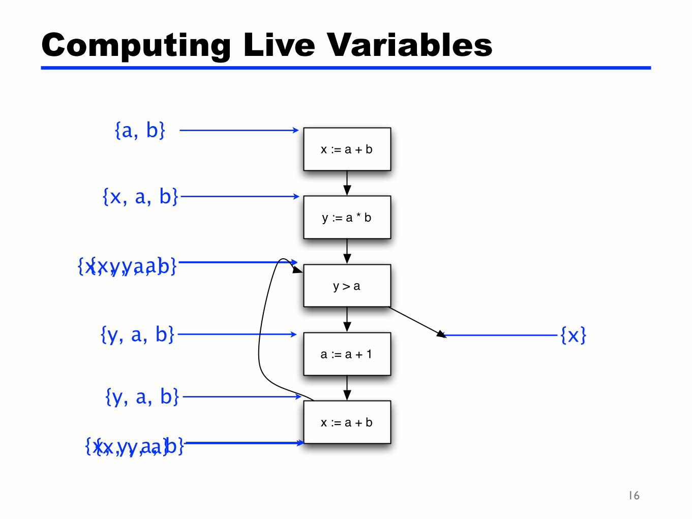
{x, y, a, b}

Computing Live Variables

{x}

{x, y, a}

{x, y, a}

{y, a, b}

{y, a, b}

{x, a, b}

{a, b}x := a + b

y := a * b

y > a

a := a + 1

x := a + b

{x, y, a, b}

17

• An expression e is very busy at point p if ■ On every path from p, expression e is evaluated before the

value of e is changed

• Optimization ■ Can hoist very busy expression computation

• What kind of problem? ■ Forward or backward? ■ May or must?

Very Busy Expressions

backward

must

18

• A definition of a variable v is an assignment to v • A definition of variable v reaches point p if

■ There is no intervening assignment to v

• Also called def-use information

• What kind of problem? ■ Forward or backward? ■ May or must?

Reaching Definitions

forward

may

19

• Most data flow analyses can be classified this way ■ A few don’t fit: bidirectional analysis

• Lots of literature on data flow analysis

Space of Data Flow Analyses

May Must

Forward Reaching definitions

Available expressions

Backward Live variables

Very busy expressions

Solving data flow equations

• Let’s start with forward may analysis ■ Dataflow equations:

- in(s) = ∪s′ ∈ pred(s) out(s′)

- out(s) = gen(s) ∪ (in(s) - kill(s))

• Need algorithm to compute in and out at each stmt • Key observation: out(s) is monotonic in in(s)

■ gen(s) and kill(s) are fixed for a given s ■ If, during our algorithm, in(s) grows, then out(s) grows ■ Furthermore, out(s) and in(s) have max size

• Same with in(s) ■ in terms of out(s’) for precedessors s’

20

Solving data flow equations (cont’d)

• Idea: fixpoint algorithm ■ Set out(entry) to emptyset

- E.g., we know no definitions reach the entry of the program

■ Initially, assume in(s), out(s) empty everywhere else, also ■ Pick a statement s

- Compute in(s) from predecessors’ out’s

- Compute new out(s) for s

■ Repeat until nothing changes

• Improvement: use a worklist ■ Add statements to worklist if their in(s) might change ■ Fixpoint reached when worklist is empty

21

22

Forward May Data Flow Algorithm

out(entry) = ∅ for all other statements s out(s) = ∅ W = all statements // worklist while W not empty take s from W in(s) = ∪s′∈pred(s) out(s′)

temp = gen(s) ∪ (in(s) - kill(s)) if temp ≠ out(s) then out(s) = temp W := W ∪ succ(s) end end

Generalizing

23

May Must

Forward

in(s) = ∪s′ ∈ pred(s) out(s′)

out(s) = gen(s) ∪ (in(s) - kill(s))

out(entry) = ∅

initial out elsewhere = ∅

in(s) = ∩s′ ∈ pred(s) out(s′)

out(s) = gen(s) ∪ (in(s) - kill(s))

out(entry) = ∅

initial out elsewhere = {all facts}

Backward

out(s) = ∪s′ ∈ succ(s) in(s′)

in(s) = gen(s) ∪ (out(s) - kill(s))

in(exit) = ∅

initial in elsewhere = ∅

out(s) = ∩s′ ∈ succ(s) in(s′)

in(s) = gen(s) ∪ (out(s) - kill(s))

in(exit) = ∅

initial out elsewhere = {all facts}

24

Forward Analysis

out(entry) = ∅ for all other statements s out(s) = all facts W = all statements while W not empty take s from W in(s) = ∩s′∈pred(s) out(s′)

temp = gen(s) ∪ (in(s) - kill(s)) if temp ≠ out(s) then out(s) = temp W := W ∪ succ(s) end end

out(entry) = ∅ for all other statements s out(s) = ∅ W = all statements // worklist while W not empty take s from W in(s) = ∪s′∈pred(s) out(s′)

temp = gen(s) ∪ (in(s) - kill(s)) if temp ≠ out(s) then out(s) = temp W := W ∪ succ(s) end end

May Must

25

Backward Analysis

in(exit) = ∅ for all other statements s in(s) = ∅ W = all statements while W not empty take s from W out(s) = ∪s′∈succ(s) in(s′)

temp = gen(s) ∪ (out(s) - kill(s)) if temp ≠ in(s) then in(s) = temp W := W ∪ pred(s) end end

in(exit) = ∅ for all other statements s in(s) = all facts W = all statements while W not empty take s from W out(s) = ∩s′∈succ(s) in(s′)

temp = gen(s) ∪ (out(s) - kill(s)) if temp ≠ in(s) then in(s) = temp W := W ∪ pred(s) end end

May Must

26

• Represent set of facts as bit vector ■ Facti represented by bit i

■ Intersection = bitwise and, union = bitwise or, etc

• “Only” a constant factor speedup ■ But very useful in practice

Practical Implementation

Generalizing Further

• Observe out(s) is a function of out(s’) for preds s’

■ We can define other kinds of functions, to compute other kinds of information using dataflow analysis!

• Example: constant propagation ■ Facts — variable x has value n (at this program point) ■ Not quite gen/kill:

- Fact that x is 3 not determined syntactically by statement

- So, how can we use data flow analysis to handle this case?

27

out(s) = gen(s) ∪ ((∪s′ ∈ pred(s) out(s′)) - kill(s))

/* facts: a = 1, b = 2 */

x = a + b

/* facts: a = 1, b = 2, x = 3 */

28

• To generalize data flow analysis, need to introduce two mathematical structures: ■ Partial orders ■ Lattices

• A partial order (p.o.) is a pair (P, ≤) such that ■ ≤ ⊆ P × P ■ ≤ is reflexive: x ≤ x ■ ≤ is anti-symmetric: x ≤ y and y ≤ x ⇒ x = y

■ ≤ is transitive: x ≤ y and y ≤ z ⇒ x ≤ z

Partial Orders

Examples

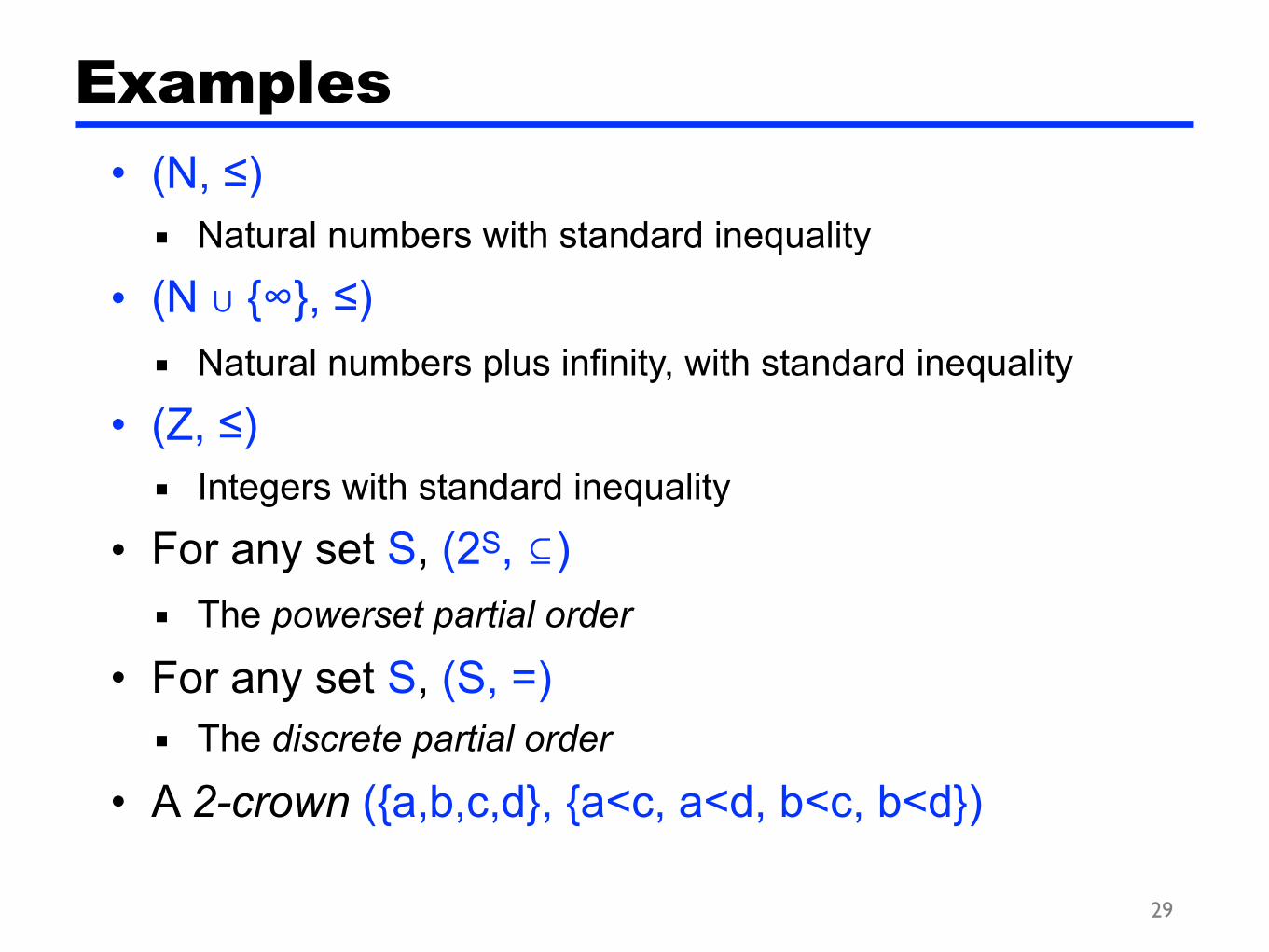
• (N, ≤) ■ Natural numbers with standard inequality

• (N ∪ {∞}, ≤) ■ Natural numbers plus infinity, with standard inequality

• (Z, ≤) ■ Integers with standard inequality

• For any set S, (2S, ⊆) ■ The powerset partial order

• For any set S, (S, =) ■ The discrete partial order

• A 2-crown ({a,b,c,d}, {a<c, a<d, b<c, b<d})

29

Drawing Partial Orders

• We can write partial orders as graphs using the following conventions ■ Nodes are elements of the p.o. ■ Edge from element lower on page to high on page means

lower element is strictly less than higher element

30

0

1

2

.

.

.

(N, ≤)0

1

2

.

.

.

∞

(N ∪ {∞}, ≤)

0

1

2

.

.

.

-1

-2

.

.

.(Z, ≤)

Drawing Partial Orders (cont’d)

31

∅

a b c

a,b a,c

a,b,c

b,c

({a,b,c}, ⊆)

a b c

({a,b,c}, =)

c d

a b

2-crown

32

• ⊓ is the meet or greatest lower bound operation:

■ x ⊓ y ≤ x and x ⊓ y ≤ y

■ if z ≤ x and z ≤ y then z ≤ x ⊓ y

• ⊔ is the join or least upper bound operation:

■ x ≤ x ⊔ y and y ≤ x ⊔ y

■ if x ≤ z and y ≤ z then x ⊔ y ≤ z

Meet and Join Operations

Examples

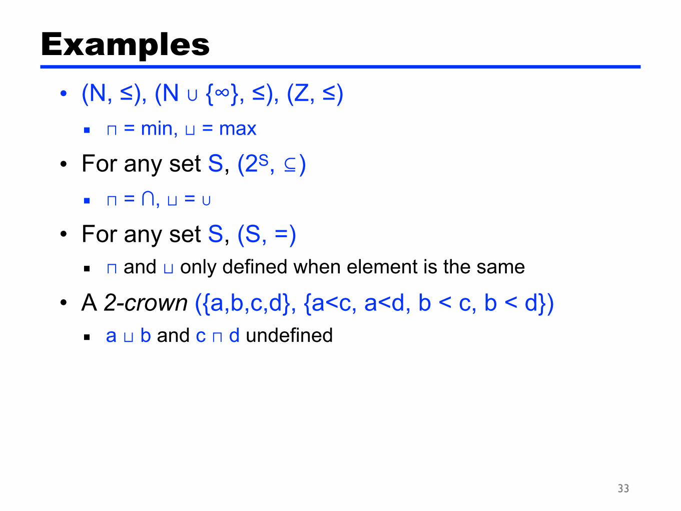
• (N, ≤), (N ∪ {∞}, ≤), (Z, ≤) ■ ⊓ = min, ⊔ = max

• For any set S, (2S, ⊆) ■ ⊓ = ∩, ⊔ = ∪

• For any set S, (S, =) ■ ⊓ and ⊔ only defined when element is the same

• A 2-crown ({a,b,c,d}, {a<c, a<d, b < c, b < d}) ■ a ⊔ b and c ⊓ d undefined

33

34

• A p.o. is a lattice if ⊓ and ⊔ are defined on any two elements ■ A partial order is a complete lattice if ⊓ and ⊔ are defined on

any set

• A lattice has unique elements ⊥ (“bottom”) and ⊤ (“top”) such that ■ x ⊓ ⊥ = ⊥ x ⊔ ⊥ = x ■ x ⊓ ⊤ = x x ⊔ ⊤ = ⊤

• In a lattice, ■ x ≤ y iff x ⊓ y = x ■ x ≤ y iff x ⊔ y = y

Lattices

Examples

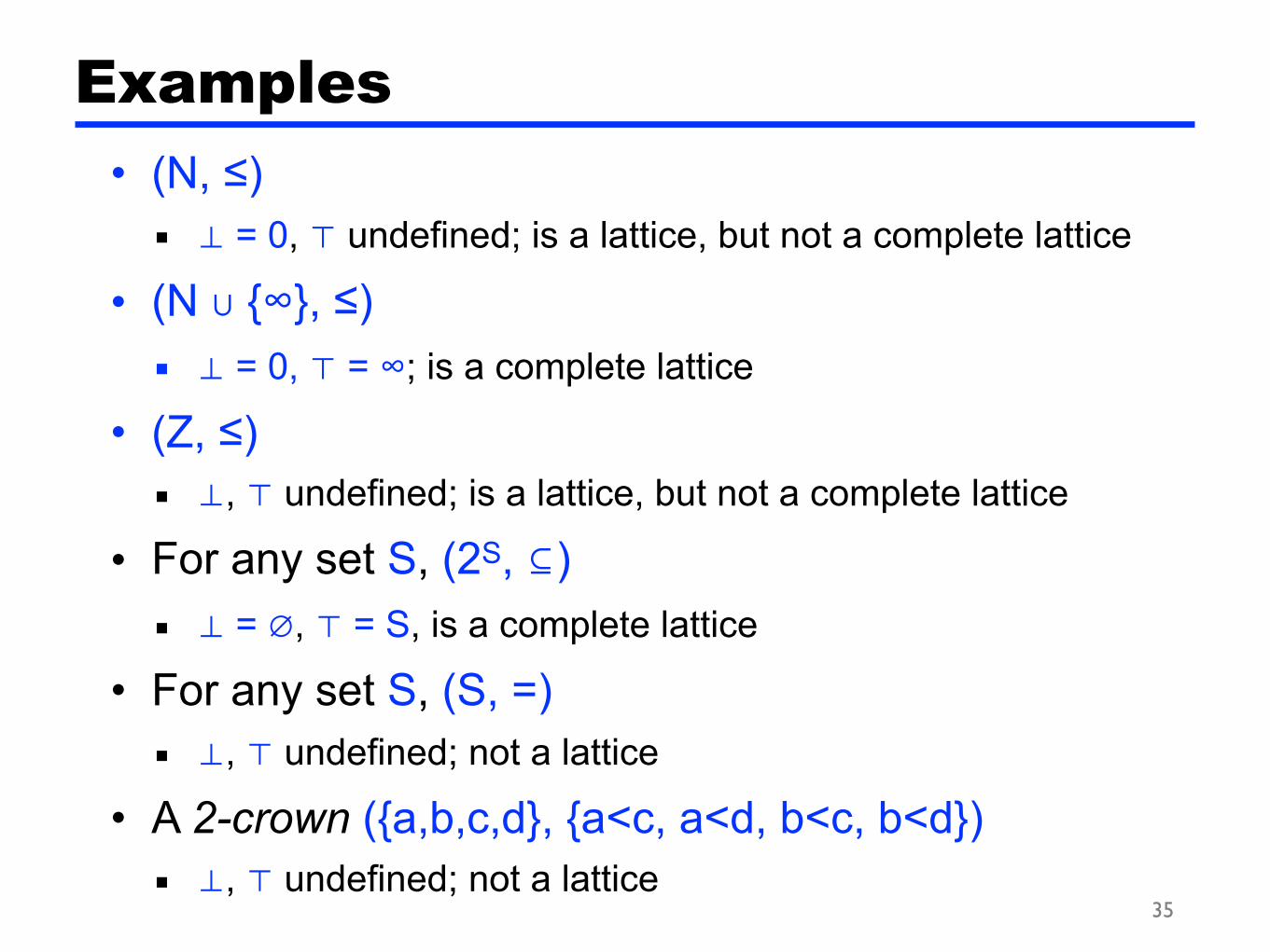
• (N, ≤) ■ ⊥ = 0, ⊤ undefined; is a lattice, but not a complete lattice

• (N ∪ {∞}, ≤) ■ ⊥ = 0, ⊤ = ∞; is a complete lattice

• (Z, ≤) ■ ⊥, ⊤ undefined; is a lattice, but not a complete lattice

• For any set S, (2S, ⊆) ■ ⊥ = ∅, ⊤ = S, is a complete lattice

• For any set S, (S, =) ■ ⊥, ⊤ undefined; not a lattice

• A 2-crown ({a,b,c,d}, {a<c, a<d, b<c, b<d}) ■ ⊥, ⊤ undefined; not a lattice

35

Flipping a Lattice

• Lemma: If (P, ≤) is a lattice, then (P, λxy.y ≤ x) is also a lattice ■ I.e., if we flip the sense of ≤, we still have a lattice

• Examples:

36

(N, ≥) ({a,b,c}, ⊇)

0

1

2

.

.

.a,b,c

a,b a,c b,c

a b

∅

c

Cross-product lattice

• Lemma: Suppose (P, ≤1) and (Q, ≤2) are lattices. Then (P×Q, ≤) is also a lattice, where ■ (p,q) ≤ (p’, q’) iff p ≤1 p’ and q ≤2 q’ ■ (Can also take cross product of more than 2 lattices, in the

natural way)

• Examples:

37

a

b

c

d

(b,c)

(b,d)

(a,c)

(a,d)× =

(b,c)

(b,d)

(a,c)

(a,d)

e

f

×

(a,c,e)

(a,c,f) (b,c,e) (a,d,e)

(b,c,f) (a,d,f)

(b,d,f)

(b,d,e)=

38

• Sets of dataflow facts form the powerset lattice ■ Example: Available expressions

Data Flow Facts and Lattices

a+b, a*b, a+1

a+b, a*b a+b, a+1

a+b

a*b, a+1

a*b a+1

(none)

Transfer Functions

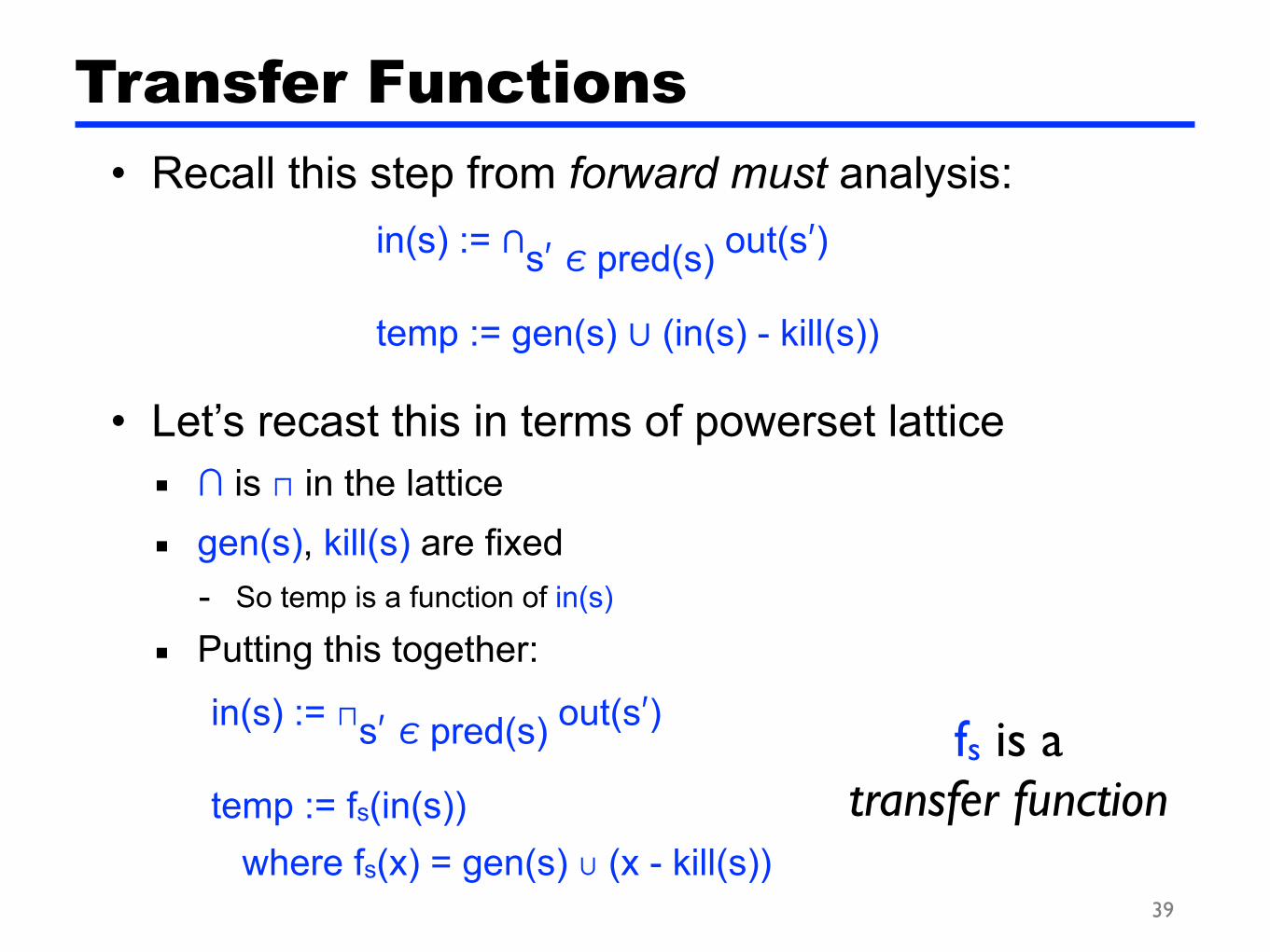
• Recall this step from forward must analysis:

• Let’s recast this in terms of powerset lattice ■ ∩ is ⊓ in the lattice ■ gen(s), kill(s) are fixed

- So temp is a function of in(s)

■ Putting this together:

39

in(s) := ∩s′ ∊ pred(s) out(s′)

temp := gen(s) ∪ (in(s) - kill(s))

in(s) := ⊓s′ ∊ pred(s) out(s′)

temp := fs(in(s)) where fs(x) = gen(s) ∪ (x - kill(s))

fs is atransfer function

Forward May Analysis

• What about forward may analysis?

■ We can just use the flipped powerset lattice - ∪ is ⊓ is that lattice

■ So we get the same equations

• Same idea for must/may backward analysis ■ But still separate from forward analysis 40

in(s) := ∪s′ ∊ pred(s) out(s′)

temp := gen(s) ∪ (in(s) - kill(s))

in(s) := ⊓s′ ∊ pred(s) out(s′)

temp := fs(in(s)) where fs(x) = gen(s) ∪ in(s) - kill(s)

Initial Facts

• Recall also from forward must analysis:

• Values of these in lattice terms depends on analysis ■ Available expressions

- out(entry) is the same as ⊥

- initial out elsewhere is the same as ⊤

■ Reaching definitions (with ≤ as ⊇) - out(entry) is ∅ which is ⊤ in this lattice (flipped powerset)

- initial out elsewhere is also ⊤

41

out(entry) = ∅ initial out elsewhere = {all facts}

Data Flow Analysis, over Lattices

42

out(entry) = (as given) for all other statements s out(s) = ⊤ W = all statements // worklist while W not empty take s from W in(s) = ⊓s′∈pred(s) out(s′)

temp = fs(in(s)) if temp ≠ out(s) then out(s) = temp W := W ∪ succ(s) end end

in(exit) = (as given) for all other statements s in(s) = ⊤ W = all statements while W not empty take s from W out(s) = ⊓s′∈succ(s) in(s′)

temp = fs(out(s)) if temp ≠ in(s) then in(s) = temp W := W ∪ pred(s) end end

Forward Backward(Red = varies by analysis)

DFA over Lattices, cont’d

• A dataflow analysis is defined by 4 things: ■ Forward or backward ■ The lattice

- Data flow facts

- ⊓ operation

- In terms of gen/kill dfa, this specifies may or must

- ⊤ value

- In terms of gen/kill dfa, this specifies the initial facts assumed at each statement

■ Transfer functions - In terms of gen/kill dfa, this defines gen and kill

■ Facts at entry (for forward) or exit (for backward) - In terms of gen/kill dfa, this defines set of facts for entry or exit node

43

44

Four Analyses as Lattices (P, ≤)

• Available expressions ■ Forward analysis ■ P = sets of expressions ■ S1 ⊓ S2 = S1 ∩ S2

■ Top = set of all expressions ■ Entry facts = ∅ = no expressions available at entry

• Reaching Definitions ■ Forward analysis ■ P = set of definitions (assignment statements) ■ S1 ⊓ S2 = S1 ∪ S2

■ Top = empty set ■ Entry facts = ∅ = no definitions reach entry

45

Four Analyses as Lattices (P, ≤)

• Very busy expressions ■ Backward analysis ■ P = sets of expressions ■ S1 ⊓ S2 = S1 ∩ S2

■ Top = set of all expressions ■ Exit facts = ∅ = no expressions busy at exit

• Live variables ■ Backward analysis ■ P = set of variables ■ S1 ⊓ S2 = S1 ∪ S2

■ Top = empty set ■ Exit facts = ∅ = no variables live at exit

Constant Propagation

• Idea: maintain possible value of each variable

- ⊤ = initial value = haven’t seen assignment to a yet

- ⊥= multiple different possible values for a

• DFA definition: ■ Forward analysis ■ Lattice = La × Lb × ... (for all variables in program)

- I.e., maintain one possible value of each variable

■ Initial facts (at entry) = ⊤ (variables all unassigned)

46

a=-1 a=0 a=1 ......

⊥

⊤

La =

Monotonicity and Desc. Chain

• A function f on a partial order is monotonic (or order preserving) if

■ Examples - λx.x+1 on partial order (Z, ≤) is monotonic

- λx.-x on partial order (Z, ≤) is not monotonic

• Transfer functions in gen/kill DFA are monotonic ■ temp = gen(s) ∪ (in(s) - kill(s))

- Holds because gen(s) and kill(s) are fixed

- Thus, if we shrink in(s), temp can only shrink

• A descending chain in a lattice is a sequence ■ x0 ⊐x1 ⊐x2 ⊐... ■ Height of lattice = length of longest descending chain

47

x ≤ y ⇒ f(x) ≤ f(y)

Monotonicity and Transfer Fns

• If fs is monotonic, how often can we apply this step?

■ Claim: out(s) only shrinks - Proof: out(s) starts out as ⊤

- Assume out(s′) shrinks for all predecessors s′ of s

- Then ⊓s′ ∊ pred(s) out(s′) shrinks

- Since fs monotonic, fs(⊓s′ ∊ pred(s) out(s′)) shrinks

48

in(s) = ⊓s′∈pred(s) out(s′) temp = fs(in(s))

Termination

• Suppose we have a DFA with ■ Finite height lattice ■ Monotonic transfer functions

• Then, at every step in DFA we ■ Remove a statement from the worklist, and/or ■ Strictly decrease some dataflow fact at a program point

- (By monotonicity)

- Only add new statements to worklist after strict decrease

■ ⇒ termination! (by finite height)

• Moreover, must terminate in O(nk) time ■ n = # of statements in program ■ k = height of lattice ■ (assumes meet operation takes O(1) time)

49

Both hold for gen/kill probs and constant prop}

50

Fixpoints

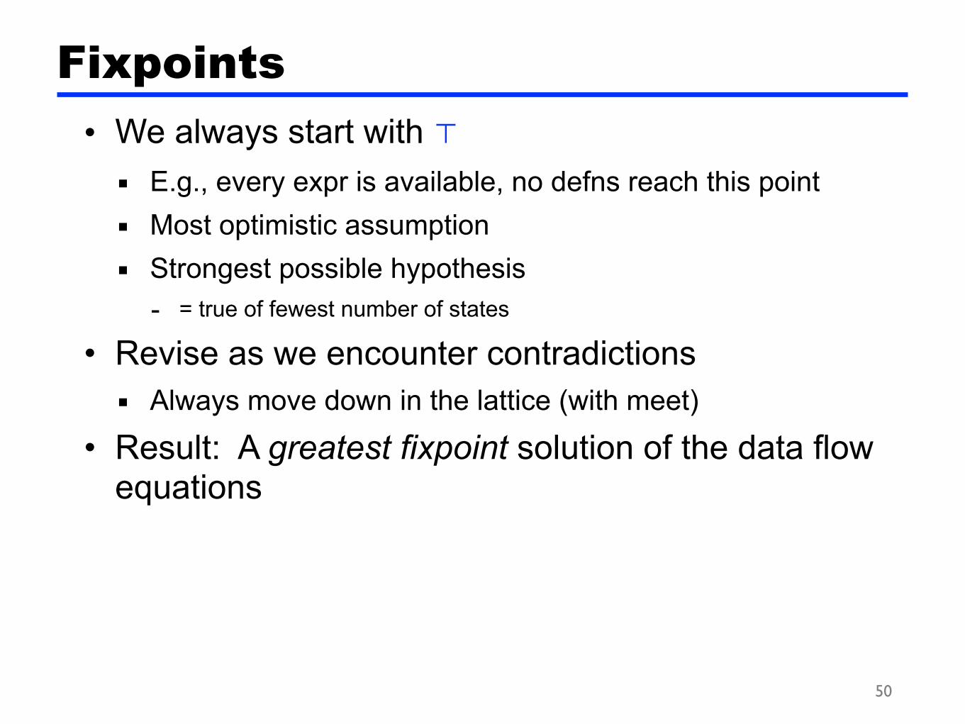
• We always start with ⊤ ■ E.g., every expr is available, no defns reach this point ■ Most optimistic assumption ■ Strongest possible hypothesis

- = true of fewest number of states

• Revise as we encounter contradictions ■ Always move down in the lattice (with meet)

• Result: A greatest fixpoint solution of the data flow equations

51

Least vs. Greatest Fixpoints

• Dataflow tradition: Start with ⊤, use ⊓ ■ Computes a greatest fixpoint ■ Technically, rather than a lattice, we only need a

- finite height meet semilattice with top

- (meet semilattice = a⊓b defined on any a,b but a⊔b may not be defined)

• Denotational semantics trad.: Start with ⊥, use ⊔ ■ Computes least fixpoint

• So, direction of DFA may depend on community author comes from...

Distributive Dataflow Problems

• A monotonic transfer function f also satisfies

■ Proof: By monotonicity, f(x ⊓ y) ≤ f(x) and f(x ⊓ y) ≤ f(y), i.e., f(x ⊓ y) is a lower bound of f(x) and f(y). But then since ⊓ is the greatest lower bound, f(x ⊓ y) ≤ f(x) ⊓ f(y).

• A transfer function f is distributive if it satisfies

■ Notice this is stronger than monotonicity

52

f(x ⊓ y) ≤ f(x) ⊓ f(y)

f(x ⊓ y) = f(x) ⊓ f(y)

Benefit of Distributivity

• Suppose we have the following CFG with four statements, a,b,c,d, with transfer fns fa, fb, fc, fd

• Then joins lose no information! ■ out(a) = fa(in(a)) ■ out(b) = fb(in(b)) ■ out(c) = fc(out(a) ⊓ out(b)) = fc(fa(in(a)) ⊓ fb(in(b)) =

fc(fa(in(a))) ⊓ fc(fb(in(b))) ■ out(d) = fd(out(c)) = fd(fc(fa(in(a))) ⊓ fc(fb(in(b))) =

fd(fc(fa(in(a)))) ⊓ fd(fc(fb(in(b)))) 53

a b

c

d

54

• Ideally, we would like to compute the meet over all paths (MOP) solution: ■ If p is a path through the CFG, let fp be the composition of

transfer functions for the statements along p

■ Let path(s) be the set of paths from the entry to s ■ Define

- I.e., MOP(s) is the set of dataflow facts if we separately apply the transfer functions along every path (assuming ⊤ is the initial value at the entry) and then apply ⊓ to the result

- This is the best we could possibly do if we want one data flow fact per program point and we ignore conditional tests along the path

• If a data flow problem is distributive, then solving the data flow equations in the standard way yields the MOP solution!

Accuracy of Data Flow Analysis

MOP(s) = ⊓p∈path(s) fp(⊤)

55

• Analyses of how the program computes ■ Live variables ■ Available expressions ■ Reaching definitions ■ Very busy expressions

• All gen/kill problems are distributive

What Problems are Distributive?

56

• Constant propagation

■ {x=1,y=2} ⊓ {x=2,y=1} = {x=⊥, y=⊥} ■ The join at in(z:=x+y) loses information ■ But in fact, z=3 every time we run this program

• In general, analysis of what the program computes in not distributive

A Non-Distributive Example

x := 1

y := 2

x := 2

y := 1

z := x + y

57

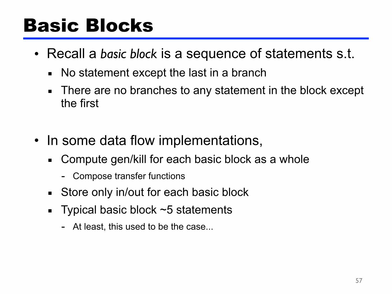
• Recall a basic block is a sequence of statements s.t. ■ No statement except the last in a branch ■ There are no branches to any statement in the block except

the first

• In some data flow implementations, ■ Compute gen/kill for each basic block as a whole

- Compose transfer functions

■ Store only in/out for each basic block ■ Typical basic block ~5 statements

- At least, this used to be the case...

Basic Blocks

58

• Assume forward data flow problem ■ Let G = (V, E) be the CFG ■ Let k be the height of the lattice

• If G acyclic, visit in topological order ■ Visit head before tail of edge

• Running time O(|E|) ■ No matter what size the lattice

Order Matters

Order Matters — Cycles

• If G has cycles, visit in reverse postorder ■ Order from depth-first search ■ (Reverse for backward analysis)

• Let Q = max # back edges on cycle-free path ■ Nesting depth ■ Back edge is from node to ancestor in DFS tree

• If ∀x.f(x) ≤ x (sufficient, but not necessary), then running time is O((Q+1)|E|) ■ Proportional to structure of CFG rather than lattice

59

60

• Data flow analysis is flow-sensitive■ The order of statements is taken into account ■ I.e., we keep track of facts per program point

• Alternative: Flow-insensitive analysis ■ Analysis the same regardless of statement order ■ Standard example: types

- /* x : int */ x := ... /* x : int */

Flow-Sensitivity

61

• What happens at a function call? ■ Lots of proposed solutions in data flow analysis literature

• In practice, only analyze one procedure at a time

• Consequences ■ Call to function kills all data flow facts ■ May be able to improve depending on language, e.g.,

function call may not affect locals

Data Flow Analysis and Functions

62

• An analysis that models only a single function at a time is intraprocedural

• An analysis that takes multiple functions into account is interprocedural

• An analysis that takes the whole program into account is whole program

• Note: global analysis means “more than one basic block,” but still within a function ■ Old terminology from when computers were slow...

More Terminology

63

• Data Flow is good at analyzing local variables ■ But what about values stored in the heap? ■ Not modeled in traditional data flow

• In practice: *x := e ■ Assume all data flow facts killed (!) ■ Or, assume write through x may affect any variable whose

address has been taken

• In general, hard to analyze pointers

Data Flow Analysis and The Heap

64

Proebsting’s Law• Moore’s Law: Hardware advances double

computing power every 18 months.

• Proebsting’s Law: Compiler advances double computing power every 18 years.

■ Not so much bang for the buck!

65

DFA and Defect Detection

• LCLint - Evans et al. (UVa) • METAL - Engler et al. (Stanford, now Coverity) • ESP - Das et al. (MSR) • FindBugs - Hovemeyer, Pugh (Maryland)

■ For Java. The first three are for C.

• Many other one-shot projects ■ Memory leak detection ■ Security vulnerability checking (tainting, info. leaks)