Embed Size (px)
Citation preview
Commutative Algebra
Tome I
Elementary properties of rings and theirmodules
Patrick Da Silva
Freie Universität Berlin
June 2, 2017


Table of Contents
Page
1 Elementary notions 81.1 Rings . . . . . . . . . . . . . . . . . . . . . . . . . . . . . . . . . . . . . . . . . . . . . . . . 81.2 Ideals . . . . . . . . . . . . . . . . . . . . . . . . . . . . . . . . . . . . . . . . . . . . . . . . 121.3 Integral domains and fields . . . . . . . . . . . . . . . . . . . . . . . . . . . . . . . . . . . 151.4 Algebras . . . . . . . . . . . . . . . . . . . . . . . . . . . . . . . . . . . . . . . . . . . . . . 181.5 Direct and inverse limits . . . . . . . . . . . . . . . . . . . . . . . . . . . . . . . . . . . . . 24
2 Operations on ideals 302.1 Intersections, sums and products . . . . . . . . . . . . . . . . . . . . . . . . . . . . . . . . 302.2 The Chinese Remainder Theorem . . . . . . . . . . . . . . . . . . . . . . . . . . . . . . . . 322.3 Ideal quotients and annihilators . . . . . . . . . . . . . . . . . . . . . . . . . . . . . . . . . 34
3 Prime, maximal and radical ideals 363.1 Prime ideals . . . . . . . . . . . . . . . . . . . . . . . . . . . . . . . . . . . . . . . . . . . . 363.2 Maximal ideals and vanishing loci . . . . . . . . . . . . . . . . . . . . . . . . . . . . . . . 383.3 Radicals . . . . . . . . . . . . . . . . . . . . . . . . . . . . . . . . . . . . . . . . . . . . . . 403.4 Prime Avoidance Lemma . . . . . . . . . . . . . . . . . . . . . . . . . . . . . . . . . . . . . 44
4 Properties of rings, part I 464.1 Euclidean domains . . . . . . . . . . . . . . . . . . . . . . . . . . . . . . . . . . . . . . . . 464.2 Greatest common divisors and GCD domains . . . . . . . . . . . . . . . . . . . . . . . . . 484.3 Principal ideal domains . . . . . . . . . . . . . . . . . . . . . . . . . . . . . . . . . . . . . 514.4 Unique factorization domains . . . . . . . . . . . . . . . . . . . . . . . . . . . . . . . . . . 524.5 Extensions and contractions . . . . . . . . . . . . . . . . . . . . . . . . . . . . . . . . . . . 544.6 Polynomial rings . . . . . . . . . . . . . . . . . . . . . . . . . . . . . . . . . . . . . . . . . 55
5 Modules 635.1 Basic operations on modules . . . . . . . . . . . . . . . . . . . . . . . . . . . . . . . . . . . 635.2 The category of modules over a ring . . . . . . . . . . . . . . . . . . . . . . . . . . . . . . 685.3 Classical results : Nakayama, Cayley-Hamilton . . . . . . . . . . . . . . . . . . . . . . . . . 78
6 Hom-functors 826.1 Basic definitions . . . . . . . . . . . . . . . . . . . . . . . . . . . . . . . . . . . . . . . . . . 826.2 Projective modules . . . . . . . . . . . . . . . . . . . . . . . . . . . . . . . . . . . . . . . . 846.3 Injective modules . . . . . . . . . . . . . . . . . . . . . . . . . . . . . . . . . . . . . . . . . 86
7 Tensor products 907.1 Adjoints to Hom functors : extension/restriction of scalars . . . . . . . . . . . . . . . . . . 907.2 Tensor product of modules . . . . . . . . . . . . . . . . . . . . . . . . . . . . . . . . . . . . 937.3 Flat modules . . . . . . . . . . . . . . . . . . . . . . . . . . . . . . . . . . . . . . . . . . . . 977.4 Tensor product of algebras . . . . . . . . . . . . . . . . . . . . . . . . . . . . . . . . . . . . 100
3

8 Localization 1038.1 The category Loc-Mod . . . . . . . . . . . . . . . . . . . . . . . . . . . . . . . . . . . . . 1038.2 Properties of rings/modules with respect to localization . . . . . . . . . . . . . . . . . . . . 111
9 Noetherian and artinian rings/modules 1229.1 Basic properties . . . . . . . . . . . . . . . . . . . . . . . . . . . . . . . . . . . . . . . . . . 1229.2 Jordan-Hölder series and modules of finite length . . . . . . . . . . . . . . . . . . . . . . . 128
10 Support and associated primes 13410.1 Support . . . . . . . . . . . . . . . . . . . . . . . . . . . . . . . . . . . . . . . . . . . . . . 13410.2 Associated primes . . . . . . . . . . . . . . . . . . . . . . . . . . . . . . . . . . . . . . . . . 13510.3 Applications . . . . . . . . . . . . . . . . . . . . . . . . . . . . . . . . . . . . . . . . . . . . 141
11 Field theory 14711.1 Irreducibility criteria . . . . . . . . . . . . . . . . . . . . . . . . . . . . . . . . . . . . . . . 14711.2 Field extensions and roots of polynomials . . . . . . . . . . . . . . . . . . . . . . . . . . . 14911.3 Algebraic extensions . . . . . . . . . . . . . . . . . . . . . . . . . . . . . . . . . . . . . . . 15611.4 Normal extensions, splitting fields and algebraic closures . . . . . . . . . . . . . . . . . . . 16211.5 Separable and inseparable polynomials . . . . . . . . . . . . . . . . . . . . . . . . . . . . . 17111.6 Cyclotomic polynomials and extensions . . . . . . . . . . . . . . . . . . . . . . . . . . . . . 179
12 Galois theory and transcendental extensions 18512.1 Separably algebraic and purely inseparable extensions . . . . . . . . . . . . . . . . . . . . 18512.2 Finite Galois extensions and the Galois group . . . . . . . . . . . . . . . . . . . . . . . . . 19812.3 Topological groups . . . . . . . . . . . . . . . . . . . . . . . . . . . . . . . . . . . . . . . . 20712.4 Inverse limits of groups . . . . . . . . . . . . . . . . . . . . . . . . . . . . . . . . . . . . . . 22012.5 Inverse limits and profinite groups . . . . . . . . . . . . . . . . . . . . . . . . . . . . . . . 22612.6 Arbitrary Galois extensions and the Krull topology . . . . . . . . . . . . . . . . . . . . . . 231
13 Transcendental Field Extensions 23613.1 Transcendental extensions . . . . . . . . . . . . . . . . . . . . . . . . . . . . . . . . . . . . 23613.2 Separable extensions . . . . . . . . . . . . . . . . . . . . . . . . . . . . . . . . . . . . . . . 24513.3 Rationality of vector spaces with respect to a field extension . . . . . . . . . . . . . . . . . 25113.4 Norms, Traces and Determinants . . . . . . . . . . . . . . . . . . . . . . . . . . . . . . . . 260
14 Cohen-Seidenberg theory 26814.1 Local rings and semilocal rings . . . . . . . . . . . . . . . . . . . . . . . . . . . . . . . . . 26814.2 Integral extensions . . . . . . . . . . . . . . . . . . . . . . . . . . . . . . . . . . . . . . . . 27114.3 Cohen-Seidenberg morphisms . . . . . . . . . . . . . . . . . . . . . . . . . . . . . . . . . . 274
15 Primary decomposition 28215.1 Primary decomposition of ideals in a ring . . . . . . . . . . . . . . . . . . . . . . . . . . . 28215.2 Primary decomposition of submodules of a module . . . . . . . . . . . . . . . . . . . . . . 296
16 Gradations, Filtrations and Completions 30616.1 Commutative monoids . . . . . . . . . . . . . . . . . . . . . . . . . . . . . . . . . . . . . . 30616.2 Graded rings and graded modules . . . . . . . . . . . . . . . . . . . . . . . . . . . . . . . 31016.3 Completions . . . . . . . . . . . . . . . . . . . . . . . . . . . . . . . . . . . . . . . . . . . . 32216.4 Z-graded and filtered rings/modules . . . . . . . . . . . . . . . . . . . . . . . . . . . . . . 330
17 Dimension Theory 34017.1 Basic definitions . . . . . . . . . . . . . . . . . . . . . . . . . . . . . . . . . . . . . . . . . . 340

18 Properties of rings, part II : Algebras over a field 34918.1 Zariski’s Lemma . . . . . . . . . . . . . . . . . . . . . . . . . . . . . . . . . . . . . . . . . . 34918.2 Noether normalization lemma . . . . . . . . . . . . . . . . . . . . . . . . . . . . . . . . . . 35018.3 Nullstellensatz . . . . . . . . . . . . . . . . . . . . . . . . . . . . . . . . . . . . . . . . . . . 356
19 Dedekind Domains 357


Preface
This first tome (hopefully in a series of many) introduces the notion of ring and its related notions (mor-phisms, modules, tensors, spectra, etc.). It will serve as a support for the corresponding set of notes onalgebraic geometry, so we freely use the language of category theory, which might be a bit shocking to thenew reader if he had a non-categorical introduction to group theory and is not used to seeing arrows anddiagrams everywhere. Note that the document is in constant evolution for the moment, so some sectionsare incomplete and some references have no target (they will appear as “??”). The reader is welcome tocontact the author via the contact information available on the homepage, whether it is to provide insighton some argument, suggest improvements to the document (such as putting some results in a different orderor improving an argument ; the document has been edited a lot, so some non-sense has definitely found itsway in there), or simply to contribute and add some sections.
7

Chapter 1
Elementary notions
Throughout this book, N = Z≥0def= 0, 1, · · · is the set of non-negative integers ; we write N+ = Z>0
def=
1, 2, · · · for the set of positive integers.
1.1 Rings
Definition 1.1. A non-commutative ring is a set R together with two binary operations, usually denotedby + : R×R→ R and · : R×R→ R which satisfy the following properties :
• Axioms for addition. We require that (R,+) is an abelian group. We denote its neutral element by 0Ror 0 if no confusion arises (which is generally the case).
• Axioms for multiplication. We require that (R, ·) is a semigroup, i.e. multiplication is associative.We denote this neutral element by 1R or 1 if no confusion arises (which is also generally the case).Multiplication is usually denoted by juxtaposition.
• Compatibility conditions. We require that · is distributive over +, i.e. for all r1, r2, r3 ∈ R, we have
r1(r2 + r3) = r1r2 + r1r3.
If we require that (R, ·) is a monoid (i.e. there exists a unit element for multiplication), then we obtain anon-commutative unital ring (we usually only add the adjective unital and don’t use the adjective “non-unital”). If we add the property that (R, ·) is a commutative monoid (so that multiplication is commutative),we obtain a commutative unital ring. Since we will mostly be concerned with commutative unital rings,we will call those rings and use the appropriate adjectives for the other structures (e.g. non-commutativering, non-commutative unital ring, etc.). Since we will always denote addition by + and multiplication byjuxtaposition, we simply denote a ring by its symbol, which is usually R or A (for the corresponding Frenchterm “anneau”).
A morphism of rings f : (R,+, ·) → (S,+, ·) (resp. non-commutative rings, unital rings) is a map ofsets f : R→ S satisfying the following properties :
(i) For all r1, r2 ∈ R, f(r1 + r2) = f(r1) + f(r2).
(ii) For all r1, r2 ∈ R, f(r1r2) = f(r1)f(r2).
(iii) If R,S and f are to be unital, then we assume f(1R) = 1S .
8
Elementary properties of rings and their modules
An inclusion of rings is an injective morphism of rings Rϕ−→ S, which we often denote by R ⊆
S. As with the notion of subobject in category theory, a subring is an equivalence class of inclusions
Rϕϕ−→ S where two inclusions Rϕ, R′ϕ′ are called equivalent if there is an isomorphism R→ R′ making a
commutative triangle
R R′
S
'
ϕ ϕ′
An isomorphism of rings is a bijective morphism of rings.
Remark 1.2. Given a ring R, to check that a non-empty subset S ⊆ R gives rise to a subring with theinclusion map as the morphism, it suffices to verify the three following properties :
• The sum of two elements of S is again in S
• The product of two elements in S is again in S
• 1R ∈ S.
This is because all the other properties of + and · hold in R, thus also hold in S, as long as the requiredelements (sums, products, unit element) are in S.
Convention 1.3. Let R be a ring and I a set. Suppose we are given a function f : I → R such that for all
i ∈ I , f(i)def= ai ∈ R. We will use the notation
∗∑i∈I
ai
where the ∗ as a superscript indicates that f−1(R \ 0) is a finite set ; in other words, this sum consistsof only finitely many terms, hence we don’t need to discuss infinite sums. Note that
∑∗i∈I∑∗
j∈J xi,j =∑∗(i,j)∈I×J xi,j .
Example 1.4. The sets Z,Q,R,C are all rings together with usual addition and multiplication ; the inclu-sions Z ⊆ Q ⊆ R ⊆ C are all morphisms. If x denotes a variable and R is a ring, then the set
R[[x]] =
∑i∈N
aixi
∣∣∣∣∣ ai ∈ R
is also a ring with usual addition and multiplication called the power series ring of R ; the notation∑i∈N aix
i is called a formal sum, the term “formal” referring to the fact that we are not adding the termsof the sum but only consider it as a formal expression. To define R[[x]] correctly (or in other words, to make
sense of the notion of a formal sum), we define it in a perhaps less natural way. As a set, R[[x]]def=∏n∈NR.
Under this notation, we set∑
n≥0 anxn def
= (a0, a1, · · · , an, · · · ), so in particular, xdef= (0, 1, 0, · · · , 0, · · · ).
Addition and multiplication are defined accordingly, namely∑n≥0
anxn
+
∑n≥0
bnxn
def=∑n≥0
(an+bn)xn,
∑n≥0
anxn
∑n≥0
bnxn
def=∑n≥0
(n∑k=0
akbn−k
)xn.
An important subring of this ring is the ring of polynomials in the variable x, which we denote by R[x] ;it is defined by
R[x] =
∗∑i∈N
aixi
∣∣∣∣∣ ai ∈ R
9

Chapter 1
Of course, addition and multiplication are defined by the same formulas.
An example of a morphism of rings R[x]→ R would be given by “plugging in” r ∈ R, i.e.
ϕr : R[x]→ R, ϕr
(n∑i=0
aixi
)def=
n∑i=0
airi.
A particularly interesting one is when r = 0, so that the map
ϕ0 : R[x]→ R, ϕ0
(n∑i=0
aixi
)7→ a0
is a morphism. One sees by induction on n that if R is a ring, then so is R[x1, · · · , xn], the polynomialring in n variables with coefficients in R. Letting R be any of the rings Z,Q,R or C in the examples weconsidered before, one obtains explicit examples such as Z[x] or C[x, y, z].
Example 1.5. Let R be a ring and I a set. The set of all functions f : I → R is denoted by RI and can begiven a canonical ring structure by pointwise addition and multiplication. The unit element of the ring isthe constant function equal to 1 and the zero is the constant function equal to zero. Note that even though∏n∈NR = RN as sets, the rings RN and R[[x]] are very different (because the multiplication on the two
of them are not the same). If I = [n]def= 1, 2, · · · , n is a finite set, then Rn
def= R[n] is the product of n
copies of the ring R. Instead of denoting its elements by functions f : [n] → R, we write them as n-tuples(a1, · · · , an) where f(i) = ai, i = 1, · · · , n.
Even though there is a notion of direct sum of abelian groups, the notion of direct sum of rings over a
set of arbitrary cardinality loses its interest for us ; the abelian group R⊕Idef=⊕
i∈I R ⊆ RI is a subgroup,it is closed under multiplication, but the unit element of RI does not belong to R⊕I unless I is finite (whenI is infinite, the unit element has infinitely many non-zero components, thus does not belong to the directsum). We are not interested in non-unital rings, so we do not explore this avenue.
(Differential geometry example) IfM is a (topological, C1, C2, · · · , Ck, · · · , C∞, Cω , complex) manifold,the set of (continuous, Ck, smooth, analytic, holomorphic) functions f : M → R or f : M → C is asubring of the corresponding ring RM or CM , which we denote by Ck(M,R) or Ck(M,C) (in the case ofholomorphic functions, notations can vary).
Proposition 1.6. The collection of small rings (i.e. where R is a small set) forms a category under compo-sition of functions, the category of rings. It is denoted by CRing. Similarly, the category of non-unitalcommutative rings is denoted by CRng, the category of non-commutative unital rings is denoted by Ringand the category of non-commutative non-unital rings is denoted by Rng.
Proof. The identity map idR : R → R gives an identity morphism for (R,+, ·) since properties (i), (ii),(iii) are trivially satisfied and identity functions act on the left and the right trivially on functions. As forcomposition, if f : (R1,+, ·) → (R2,+, ·) and g : (R2,+, ·) → (R3,+, ·) are morphisms, then g fsatisfies
(g f)(r1 + r2) = g(f(r1 + r2)) = g(f(r1)) + g(f(r2)) = (g f)(r1) + (g f)(r2)
(g f)(r1r2) = g(f(r1r2)) = g(f(r1)f(r2)) = g(f(r1))g(f(r2)) = (g f)(r1)(g f)(r2)
(g f)(1R1) = g(f(1R1)) = g(1R2) = 1R3 .
and thus is also a morphism. Composition of functions is of course associative, so composition ofmorphisms also is.
Definition 1.7. Let A be a ring. Define A×def= a ∈ A | ∃b ∈ A s.t. ab = 1. The set A× forms a group
with respect to multiplication ; its elements are called the units or invertible elements of A in particular, if
10

Elementary properties of rings and their modules
a ∈ A×, its inverse element is unique and is denoted by a−1. A morphism of rings f : A→ B correspondsto a morphism of groups f× : A× → B× since if aa′ = 1A, then f(a)f(a′) = f(1A) = 1B .
If Af−→ B, B
g−→ C are morphisms of rings, then (g f)× = g× f× and id×A = idA× , hence(−)× : CRing→ Grp is a functor.
Let NZD(A)def= a ∈ A | ∀b ∈ A \ 0, ab 6= 0 be the set of non-zero divisors of A and note
that A× ⊆ NZD(A), i.e. invertible elements are non-zero divisors (in some references, elements of a ring
which are non-zero divisors are called regular elements of the ring). Let ZD(A)def= a ∈ A | ∃b ∈
A \ 0 s.t. ab = 0, the set of zero divisors of A.
Example 1.8. For R = Q,R or C, we have R× = R \ 0, but Z× = −1,+1 ; however, NZD(Z) =Z \0. So even though an element of a ring can be a non-zero divisor which is not a unit, its inverse mayexist in a larger ring. We will study this phenomenon in Chapter 8.
Consider R = C0([−1, 1],R), the ring of continuous functions f : [0, 1] → R (c.f. Example 1.5. Thefunction f : [−1, 1] → R defined f(x) = x is neither a unit or a zero divisor. Let f1, f2 : [−1, 1] → R bedefined by f1(x) = maxx, 0 and f2(x) = minx, 0. Then f1f2 = 0 even though f1 6= 0 and f2 6= 0.Thus R admits zero divisors which are not zero.
Remark 1.9. It is clear that
ZD(A) ∪NZD(A) = A, ZD(A) ∩NZD(A) = ∅.
(One must take care to separate the case of the zero ring from the other rings, which we will discuss inLemma 1.10). If a ∈ NZD(A) with ab = ab′ for b, b′ ∈ A, then b = b′ (since then a(b− b′) = 0) ; this is thecancellation law for non-zero divisors. Non-zero divisors are precisely those elements of a ring for whichthe cancellation law holds.
Lemma 1.10. Let A be a ring. The following three statements are equivalent :
(i) A 6= 0
(ii) 1 6= 0
(iii) 0 ∈ NZD(A).
(iv) 0 /∈ ZD(A).
It follows that there is only one ring where 1 = 0 and it has one element ; it is called the zero ring, whichwe denote by 0.
Proof. Clearly (ii) implies (i), and if 1 = 0, then x = 1 · x = 0 · x = 0, so (i) implies (ii). Note that for anyx ∈ A,
0x = (0 + 0)x = 0x+ 0x =⇒ 0x = 0.
The equivalence of (i) & (ii) with (iii) follows because 0 ∈ ZD(A) is then equivalent to A \ 0 = ∅. Thestatements (iii) and (iv) are equivalent by Remark 1.9.
Remark 1.11. In any non-zero ring A, the zero element 0 is always a zero divisor ; we call it the trivial zerodivisor. Any other zero divisor of A is called non-trivial.
Theorem 1.12. In the category CRing, the object Z is initial and 0 is terminal. In particular, since Z 6' 0,the category CRing is not additive. Furthermore, this category is concrete, the functor U : CRing→ Setsending a morphism of rings to its underlying map of sets. Finally, a morphism of rings ϕ : A → B is anisomorphism if and only if the underlying set map U(ϕ) is bijective.
11

Chapter 1
Proof. If R is a ring, then there is a unique morphism ϕ : Z→ R given for n > 0 inductively by
ϕ(0)def= 0, ϕ(1)
def= 1, ϕ(n)
def= ϕ(n− 1) + 1
and ϕ(−n)def= −ϕ(n) for n < 0. These formulas define ϕ and must hold for a morphism of rings, so we
obtain existence and unicity.As for the zero ring, there is only one map R → 0, and since 0 = 1, it happens to be a morphism ofrings. The functor U is clearly faithful. In particular, it maps isomorphisms to bijections, so Z 6' 0.For the last statement, clearly if ϕ is an isomorphism, then it is bijective. Conversely, a bijective morphismof rings is such that the inverse map is also a morphism :
ϕ−1(b1 + b2) = ϕ−1(ϕ(ϕ−1(b1)) + ϕ(ϕ−1(b2))) = ϕ−1(ϕ(ϕ−1(b1) + ϕ−1(b2))) = ϕ−1(b1) + ϕ−1(b2)
and similarly for multiplication. That ϕ−1(1B) = 1A holds is also obvious.
Proposition 1.13. Let A be a ring. Then 02 = 0, (−1)2 = 1 and (−1)a = −a for all a ∈ A ; that is, theadditive inverse of a is a times the additive inverse of 1.
Proof. Since 02 = 0(0 + 0) = 02 + 02, 02 = 0. In particular,
0 = (1 + (−1))2 = 12 + 1(−1) + (−1)1 + (−1)2 = (−1)2 − 1 =⇒ (−1)2 = 1.
For the last property, note that a+ (−1)a = (1 + (−1))a = 0a = 0, so (−1)a = −a by the unicity of theadditive inverse.
1.2 Ideals
A big result in group theory is the fact that if ϕ : G→ H is a morphism of groups, then kerϕ is a normalsubgroup of G, imϕ is a subgroup of H and G/kerϕ ' imϕ. In the same way that not any subgroup ofa group is a normal subgroup and allows the definition of a quotient, we need to take care how we definequotients in rings. The correct class of subsets of a ring to use to define quotients is the notion of ideal,which we now introduce. One of the reasons for this is that the obvious candidate for the notion of kernelof a morphism (namely, the inverse image of 0) never contains the unit element of the ring since these needto satisfy ϕ(1) = 1 6= 0, hence this candidate cannot be a subring.
Definition 1.14. Let ϕ : A→ B be a morphism of non-commutative rings. The kernel of ϕ is the subset
kerϕdef= ϕ−1(0) = a ∈ A | ϕ(a) = 0.
Of course, if A and B are commutative or unital, we take the same definition as the kernel of the morphism.
Remark 1.15. In CRing, the kernel of a morphism is not a categorical kernel ; this is because the kernel ofa morphism of unital rings is never unital unless its codomain is zero. To treat this kernel as a categoricalkernel, we will need to introduce the category of modules over a ring, which will be done in Chapter 5.
Definition 1.16. Let A be a ring. An ideal of A is a subset a ⊆ A satisfying the two following properties :
• a ≤ A is a subgroup of (A,+)
• For all a ∈ A and b ∈ a, we have ab ∈ a.
To indicate that a is an ideal of A, we write a E A. Given an ideal a of A, one forms the quotient abeliangroup A/a. Let
(a1 + a) · (a2 + a)def= (a1a2 + a).
12

Elementary properties of rings and their modules
This is well-defined, for if y1 = x1 + a1, y2 = x2 + a2 where a1, a2 ∈ a and x1, x2, y1, y2 ∈ A, then
y1y2 = x1x2 + x1a2 + x2a1 + a1a2︸ ︷︷ ︸∈a
≡ x1x2 (mod a) =⇒ y1y2 + a = x1x2 + a.
Remark 1.17. If A is non-commutative, we need to use different definitions (which we might need onoccasion). A subset a ⊆ A is called
(a) a left ideal (resp. right ideal) if a ≤ A is an additive subgroup and for any a ∈ A, b ∈ a, we haveab ∈ a (resp. ba ∈ a)
(b) a two-sided ideal if it is both a left ideal and right ideal.
Proposition 1.18. Let a E A be an ideal. Then (A/a,+, ·) is a ring with zero element 0 + a and unitelement 1 + a. The quotient map of abelian groups πa : A→ A/a is a surjective morphism of rings.
Proof. We have already shown that multiplication is well-defined. The proof that + and · satisfy theproperties of Definition 1.1 is done by an argument which we call adding decorations ; since such aproperty holds for A, it holds when we decorate the elements with +a next to them. For instance,
(a+ a)((b+ a) + (c+ a)) = a(b+ c) + a = (ab+ a) + (ac+ a) = (a+ a)(b+ a) + (a+ a)(c+ a).
The adding decorations argument also shows that πa is a morphism. Surjectivity is obvious since for anya+ a ∈ A/a, we have a+ a = ϕa(a).
Remark 1.19. We often use the argument of adding decorations when dealing with quotients. It works forgroups, rings, later with modules (c.f. Chapter 5) and more generally any concrete category which admitsquotient objects where the quotient maps are surjective ; if some property involving equations on elementsholds on an object, then it also holds on the quotient object by adding decorations. Note that this is not aformal statement but rather a train of thought which will come back when we deal with different kinds ofmathematical objects. Arguments which need to be done by adding decorations are often trivial and left tothe reader.
Lemma 1.20. Let A be a ring and a ⊆ A a non-empty subset. Then the following are equivalent :
(i) a is an ideal of A.
(ii) For every a, b ∈ a, we have a+ b ∈ a and for every c ∈ A, we have ca ∈ a.
(iii) There exists a morphism ϕ : A→ B such that kerϕ = a.
Proof. ( (i)⇒ (iii) ) The morphism πa of Proposition 1.18 obviously satisfies kerπa = a.( (iii) ⇒ (ii) ) If a, b ∈ kerϕ, then ϕ(a + b) = ϕ(a) + ϕ(b) = 0. If c ∈ A, then ϕ(ca) = ϕ(c)ϕ(a) =ϕ(c) · 0 = 0.( (ii)⇒ (i) ) The only property left to show is that if a ∈ a, then −a ∈ a. This is clear since −a = (−1)a ∈a by property (ii) and Proposition 1.13.
Theorem 1.21. Let πa : A → A/a be the surjective morphism of Proposition 1.18. Then πa satisfies thefollowing universal property : for each morphism ϕ : A→ B such that a ⊆ kerϕ, there exists a morphismϕa : A/a→ B making the following diagram commute :
A A/a
B
ϕ
πa
ϕa
13

Chapter 1
Proof. The proof goes similarly as in the case of abelian groups. Define ϕa(a+ a)def= ϕ(a). This is well
defined since if y = x + a with a ∈ kerϕ, then ϕ(y) = ϕ(x). The fact that ϕa is a morphism followsfrom adding decorations. By definition, ϕa πa = ϕ.
Corollary 1.22. (First isomorphism theorem) Let ϕ : A→ B be a morphism of rings. Then
imϕdef= b ∈ B | ∃a ∈ A s.t. ϕ(a) = b
is a subring of B, kerϕ is an ideal of A and ϕkerϕ : A/kerϕ→ imϕ is an isomorphism.
Proof. We already know that kerϕ E A. The fact that imϕ is a subring is straightforward from Re-mark 1.2 and the definition of a morphism. By definition, ϕ maps onto imA, hence ϕkerϕ maps ontoimϕ. To see that ϕkerϕ is injective, notice that
0 = ϕkerϕ(a+ kerϕ) = ϕ(a) =⇒ a+ kerϕ = 0 + kerϕ.
Theorem 1.23. (Second isomorphism theorem) Let A be a ring, B ⊆ A a subring and a E A an ideal.
Then B+ adef= b+a | b ∈ B, a ∈ a is a subring of A, B ∩ a E B is an ideal and we have an isomorphism
(B + a)/a ' B/(B ∩ a).
Proof. It is clear that B + a ⊆ A is a subgroup. For multiplication, if b1 + a1, b2 + a2 ∈ B + a, we have
(b1 + a1)(b2 + a2) = b1b2 + a1b2 + a2b1 + a1a2︸ ︷︷ ︸∈a
∈ B + a.
Since a ⊆ B + a, it is clear that a E B + a. Similarly, it is clear that B ∩ a ⊆ B is a subgroup ; ifa ∈ B ∩ a and b ∈ B, then ab ∈ B because B is a subring and ab ∈ a because a E A. The compositionϕ : B ⊆ B + a
πa−→ (B + a)/a is surjective with kerϕ = B ∩ a, so we are done.
Lemma 1.24. Let f : A→ B be a morphism of rings and b E B. Then f−1(b) E A and f(a) ⊆ f(A)def=
im f . In particular, if f is surjective, then f(a) E B.
Proof. This follows by Lemma 1.20 in both cases. In the first case, f−1(b) = ker(Af−→ B
πb−→ B/b). Inthe second case, Lemma 1.20 (ii) makes it obvious.
Theorem 1.25. (Third isomorphism theorem) Let a ⊆ b be two ideals of a ring A. Then b/a E A/a andwe have an isomorphism (A/a)/(b/a) ' A/b.
Proof. Lemma 1.24 proves that b/a E A/a since πa : A → A/a is surjective. The composition Aπa−→
A/aπb/a−→ (A/a)/(b/a) is surjective with kernel a + b = b, so we are done by the First Isomorphism
Theorem (Corollary 1.22).
Theorem 1.26. (Lattice isomorphism theorem) Let A be a ring and a E A. There is an inclusion-preservingbijective correspondence between the sets
b E A | a ⊆ b b7→πa(b)←−−−−−−−→π−1a (c)←[c
c E A/a
14

Elementary properties of rings and their modules
Proof. By Lemma 1.24, the correspondence sends ideals in one set to ideals in the other ; it suffices toshow that this correspondence is bijective. The equation πa(π−1
a (c)) = c follows by surjectivity of πa.Clearly b ⊆ π−1
a (πa(b)) ; for the reverse inclusion, if a ∈ A satisfies πa(a) ∈ πa(b), there exists b ∈ b
with a+ a = b+ a, so that a′def= a− b ∈ a ⊆ b, hence a = a′ + b ∈ b.
Since a ⊆ b ⊆ b′ implies πa(b) ⊆ πa(b′) and c ⊆ c′ implies π−1
a (c) ⊆ π−1a (c′), the bijection is inclusion-
preserving.
Definition 1.27. We say that an ideal a E A is generated by a subset S ⊆ a if
a =
∗∑s∈S
ass
∣∣∣∣∣ as ∈ A,
or in other words, any element of A is a finite sum of elements of S multiplied by elements of A. If we canpick S finite, we say that a is finitely generated ; if we can pick S = s, we say that a is a principalideal. We write (S)A for the ideal generated by S ; in the finitely generated case, we write (s1, · · · , sn)A. Ifthe ring A is understood, we sometimes omit (S)A and simply write (S).
Example 1.28. Let A be a ring. Then every S ⊆ A generates an ideal adef= (S)A E A called the ideal
generated by S in A. In particular, every element s ∈ A generates a principal ideal ; we can write(s)A = as | a ∈ A. The fact that these are ideals follows from Lemma 1.20 (ii). Since a sum over anempty set of elements is equal to zero by convention, we have (∅)A = (0).
The ideal (0)A is called the zero ideal and is denoted by (0), or sometimes just by 0 ; it is the kernelof the identity morphism idA : A→ A. The ideal A = (1)A is the kernel of the zero morphism (to the zeroring) denoted by 0 : A→ 0. Both ideals are principal, the first generated by 0 and the second by 1. Becausethe zero ring is often not interesting, we call an ideal a E A proper if a 6= A. Note that a = A if and onlyif a contains a unit.
Lemma 1.29. Let f : A → B be a morphism. Assume a = (S)A E A and b = (T )B E B where S ⊆ a,T ⊆ b are sets of generators. Then
(f−1(T ))A + ker f ⊆ f−1(b), f(a) ⊆ (f(S))B.
If f is surjective, the inclusions become equalities.
Proof. For the inclusions, T ⊆ b implies f−1(T ) ⊆ f−1(b), thus (f−1(T ))A ⊆ f−1(b) since f−1(b) isan ideal, and clearly ker f ⊆ f−1(b) ; if a ∈ a, write a =
∑∗s∈S ass, so that f(a) =
∑s∈S f(as)f(s) ∈
(f(S))B , proving that f(a) ⊆ (f(S))B .If f is surjective, assume f(a) ∈ b = (T )B and write f(a) =
∑∗t∈T btt. Picking st ∈ f−1(T ) such that
f(st) = t and at ∈ A such that f(at) = bt, it follows that f(a) = f(∑∗
t∈T atst), i.e. a −
∑∗t∈T atst ∈
ker f . For the second equality, write b ∈ (f(S))B as b =∑∗
s∈S bsf(s) and find as ∈ A such thatf(as) = bs, so that b = f
(∑∗s∈S ass
)∈ f((S)A) = f(a).
Remark 1.30. The addition ker f in Lemma 1.29 is necessary for the equalities to hold ; just consider thecase T = ∅, so that (f−1(T ))A = (0)A 6= ker f . However, we can always re-write (f−1(T ))A + ker f =(f−1(T ∪ 0))A.
1.3 Integral domains and fields
If n ∈ Z is an integer, it is standard to write nZ def= (n)Z ; it consists of all integer multiples of n. Since
(n)Z = (−n)Z, it is standard to assume in the notation nZ that n ≥ 0. The ring Z/nZ is the ring structure
15

Chapter 1
on the finite cyclic group given by multiplication of integers modulo n : for a, b ∈ Z,
(a+ nZ)(b+ nZ)def= ab+ nZ .
Definition 1.31. Let iA : Z→ A be the unique morphism of rings given by Theorem 1.12. Since ker iA E Z,there is a unique n ≥ 0 such that ker iA = nZ (since in particular, ker iA ≤ Z is a subgroup). The integer nis called the characteristic of the ring, which is denoted by ch(A).
Remark 1.32. The rings Z/nZ have characteristic n ; the zero ring is the unique ring with characteristic 1.In general, if ch(A) = 0, then adding 1 with itself n times gives a non-zero element of A for all n > 0. Ifch(A) > 1, then ch(A) is the smallest positive integer for which
1 + . . .+ 1︸ ︷︷ ︸n times
= 0.
Definition 1.33. Let A be a ring. An element a ∈ A is called nilpotent if there exists n > 0 such that
andef= a · . . . · a︸ ︷︷ ︸
n times
= 0 (by convention, we set a0 def= 1 for any a ∈ A, including the case a = 0). The set of all
nilpotent elements of A is denoted by Nil(A).
The ring A is called
• an integral domain if NZD(A) = A \ 0 ; in other words, the non-zero elements of A are preciselythe non-zero divisors
• a field if A× = A \ 0 ; in other words, the units of A are its non-zero elements
• reduced if Nil(A) = (0) (c.f. Proposition 1.37, where we show that Nil(A) E A).
Remark 1.34. Note that the zero ring A = 0 is not an integral domain or a field : NZD(A) = 0 = A×
and A \ 0 = ∅. The rings Z,Q,R and C are all integral domains ; the rings Q,R and C are fields.
If A is an integral domain and B ⊆ A is a subring, then B is also an integral domain ; this follows bydefinition. The converse is not true : a non-integral domain may contain an integral domain as a subring.Consider A[x, y]/(xy) where A is an integral domain ; the inclusion map A → A[x, y]/(xy) shows that Ais an integral domain and a subring of A[x, y]/(xy), but (x+ (xy))(y+ (xy)) = xy+ (xy) = 0 in this ring,so it is not an integral domain.
If A 6= 0 is a ring, then Nil(A) 6= A ; this is because 1 ∈ A is never nilpotent.
Example 1.35. Let A be a ring and pick a ∈ A\0. If A is an integral domain, the powers a, a2, · · · , an, · · ·are all distinct, for if am = an with m ≥ n, the cancellation law implies am−n = 1, i.e. m = n. On the
other hand, for any ring A and n ≥ 2, the ring Bdef= A/(an) admits non-zero nilpotents, namely am + (an)
for 0 < m < n.
Let n > 0 be an integer and write its prime factorization as n = pa11 . . . pakk . If m is an integer such that
p1 · · · pk divides m, then m+nZ is nilpotent in Z/nZ ; the integer m` will become a multiple of n preciselywhen ` is greater than all the ai’s, thus (m+ nZ)` = 0.
Remark 1.36. For A 6= 0, we have
0 ⊆ Nil(A) ⊆ ZD(A) ⊆ A \A× ⊆ A
and1 ⊆ A× ⊆ NZD(A) ⊆ A \Nil(A) ⊆ A.
(For A = 0, ZD(A) = ∅ and A = Nil(A), hence A \Nil(A) = ∅.)
16

Elementary properties of rings and their modules
Proposition 1.37. Let A be a ring. The subset Nil(A) ⊆ A is an ideal of A. We call it the nilradical of A.Furthermore, the ring
Areddef= A/Nil(A)
is reduced, i.e. Nil(Ared) = 0.
Proof. We use Lemma 1.20 (ii). Suppose a, b ∈ Nil(A) satisfy an = 0 and bm = 0. Then by Lemma 1.45,
(a+ b)n+m =
n+m∑k=0
(n+m
k
)akbm+n−k
= bm
(n∑k=0
(n+m
k
)akbn−k
)+ an
(m∑
k=n+1
(n+m
k
)ak−nbn+m−k
)= 0
and (ca)n = cnan = 0. To see the last statement,
0 = (a+ Nil(A))n = an + Nil(A) =⇒ an ∈ Nil(A) =⇒ a ∈ Nil(A)
since anm = (an)m = 0. (This last implication is the fact that the nilradical of A is a radical ideal ; seeProposition 3.20 (h).)
Proposition 1.38. Let A 6= 0 be a ring. If x ∈ Nil(A) and y ∈ A×, then x + y ∈ A×. In particular,1 + x, 1− x ∈ A×.
Proof. We can write x + y = y(y−1x + 1) and y−1x ∈ Nil(A), so without loss of generality we canassume y = 1. Since Nil(A) is an ideal, we can replace x by −x and prove without loss of generality that1− x ∈ A×. Letting n ≥ 1 be such that xn = 0, we have
1 = 1− xn =n−1∑i=0
xi −n∑i=1
xi = (1− x)
(n−1∑i=0
xi
).
Proposition 1.39. Let A be an integral domain of characteristic pdef= ch(A) > 1. Then p is a prime number,
i.e. if ab = p where a, b are positive integers, then either a or b is a multiple of p.
Proof. Let iA : Z→ A be the morphism of Theorem 1.12 and assume ab = p as in the statement. UsingTheorem 1.21, obtain the injective morphism iA,p : Z/pZ → A. Since this makes Z/pZ a subring of R,Z/pZ is an integral domain. The equation
iA,p(a+ pZ)iA,p(b+ pZ) = iA,p(ab+ pZ) = iA(p) = 0
implies iA(a) = 0 or iA(b) = 0, which means a ∈ pZ or b ∈ pZ.
Theorem 1.40. Let A be a finite integral domain. Then A is a field.
Proof. Let a ∈ A \ 0. The map of sets fa : A → A defined by b 7→ ab is injective by the cancellationlaw for a since A \ 0 = NZD(A). Since A is finite, it is bijective. Therefore there exists b ∈ A withab = 1, showing that A× = A \ 0.
Corollary 1.41. The finite ring Z/nZ is an integral domain (resp. field) if and only if n is a prime number.
17

Chapter 1
Proof. (⇒) If n is not a prime number, write n = ab for 1 < a, b < n. Then (a + nZ)(b + nZ) = 0in Z/nZ, showing that Z/nZ is not an integral domain (note that the choice 1 < a, b < n implies thata+ nZ 6= 0 6= b+ nZ).(⇐) This follows from Proposition 1.39 and Theorem 1.40.
Definition 1.42. Let p ∈ N be a prime number. We write Fpdef= Z/pZ for the finite field with p elements.
Example 1.43. We exhibit a few properties of the finite rings Z/nZ :
(a) Z× = 1,−1, ZD(Z) = 0, NZD(Z) = Z \0, Nil(Z) = 0.
(b) A = Z/6Z, A× = 1, 5 = NZD(A), ZD(A) = 0, 2, 3, 4, Nil(A) = 0.
(c) A = Z/4Z, A× = 1, 3 = NZD(A), ZD(A) = 0, 2, Nil(A) = 0, 2.
From (b) we see that in general, ZD(A) is not an ideal.
Proposition 1.44. Let A 6= 0 be a ring. Then the following are equivalent :
(i) A is a field
(ii) The only ideals of A are 0 and A
(iii) Every non-zero morphism of rings ϕ : A→ B is injective.
(iv) The set A \ 0 becomes a group under multiplication.
Proof. ( (i)⇒ (ii) ) If a E A is not the zero ideal, let a ∈ a \ (0) ⊆ A \ (0) = A×. Letting b ∈ A such thatba = 1, we see that 1 ∈ a, showing that a = A.( (ii) ⇒ (iii) ) Suppose ϕ : A → B is non-zero. Then kerϕ 6= A, hence kerϕ = 0. This means ϕ isinjective.
( (iii) ⇒ (i) ) Let a ∈ A − A×. Since a is not a unit, adef= (a)A E A is a proper ideal, so A/a is not the
zero ring. By hypothesis, the map πa : A→ A/a is injective, therefore a = 0.( (i) ⇐⇒ (iv) ) Under both conditions (i) and (iv), A is an integral domain, so we can assume A \ 0 is amonoid. Since a monoid is a group if and only if every of its elements admits an inverse, we are done.
Lemma 1.45. Let a, b ∈ A and n ≥ 0 an integer. For 0 ≤ i ≤ n, set(ni
) def= n!
i!(n−i)! , called the binomialcoefficient (pronounced “n choose i” because of its combinatorial properties). Then
(a+ b)n =n∑i=0
(n
i
)aibn−i.
Proof. By induction on n. The proof is no different than with real numbers, so we omit it.
1.4 Algebras
Definition 1.46. A triple (R,A, ϕ : R → A) where ϕ is a morphism of rings is called a commutativeR-algebra, hence the name of the theory. We also say that A is a (commutative) algebra over R. Forbrevity, when we assume that A is a commutative unital ring (as we do), we call such a triple an R-algebra.
18

Elementary properties of rings and their modules
A morphism of R-algebras from (R,A, ϕ) to (R,A′, ϕ′) is a morphism of rings ψ : A → A′ making acommutative triangle
R
A A′
ϕ ϕ′
ψ
or in other words, ψ ϕ = ϕ′.
Remark 1.47. One sees using such diagrams that the R-algebras together with morphisms of R-algebrasform a subcategory of CRing, namely the category of R-algebras which we denote by R-Alg. The diagrammakes it obvious that this corresponds to the comma category (R ↓ CRing). The R-algebra structure of aring is often implicit in practice, hence unless it seems necessary, we only denote a triple (R,A, ϕ : R→ A)by A and mention it is an R-algebra if we use its R-algebra structure. Note that the categories CRing andZ -Alg are canonically isomorphic (sending a ring R to the Z-algebra (Z, R, iZ : Z→ R)) since Z is initialin CRing.
Let R be a ring and X an abelian group. A linear ring action of R on X is a map · : R ×X → Xsatisfying the following axioms :
• For all r1, r2 ∈ R and a ∈ A, we have (r1 + r2) · a = r1 · a+ r2 · a
• For all r ∈ R and a1, a2 ∈ A, we have r · (a1 + a2) = r · a1 + r · a2
• For all r1, r2 ∈ R and a ∈ A, we have r1 · (r2 · a) = (r1r2) · a
• For all a ∈ A, we have 1R · a = a.
If ϕ : R→ A is a morphism of rings, then ϕ and the multiplication in A gives A the structure of a linearring action. We call this action the induced linear ring action of R on A by ϕ. It is not hard to check thatthe notion of a linear ring action · : R ×X → X is equivalent to a morphism of non-commutative unitalrings R → HomZ(X,X) where HomZ(X,X) is a non-commutative unital ring under pointwise additionand composition of functions. Under this notation, a morphism of R-algebras ψ : A → A′ is a morphismwhich commutes with the action of R, i.e. ψ(r · a) = r · ψ(a) for all r ∈ R and a ∈ A.
Suppose X is an abelian group with two linear ring actions, · : A × X → X and : R × X → X ;furthermore, assume ϕ : R → A makes A into an R-algebra. The linear ring action · : A × X → X iscalled R-linear if for all r ∈ R, the two actions agree, namely r x = ϕ(r) · x. If R = Z, we note that anylinear ring action is Z-linear. Examples of R-linear actions will happen very often when we study modulesover R-algebras in Chapter 5.
Note that the morphism ϕ : R→ A is not required to be injective, so that the notation r · a should notlead to believe that ϕ(r) 6= 0. We usually drop the dot and write ra for ϕ(r)a ; this choice of notation willbecome clearer in the context of modules (c.f. Chapter 5).
Example 1.48. Let F be a field and A an F -algebra. Since any morphism of rings F → A is injective, wecan characterize F -algebras as those which contain F as a subfield (a subfield is a subring which is a field).This is a particular situation for algebras over a field ; in general, morphisms of rings may have non-trivialkernels, so that an R-algebra A might not contain R as a subring but rather a quotient of it, i.e. R/a ⊆ Afor a the kernel of the morphism R→ A defining the algebra.
The last result of this section will require a bit of work but will be worth its while. In commutativealgebra, it is often the case that one deals with polynomial rings in several variables. Considering the setof variables x1, · · · , xn, one obtains a commutative monoid consisting of all expressions of the form
19

Chapter 1
xi11 · · ·xinn with i1, · · · , in ∈ N. In a more general setting, one can consider generators of a commutativemonoid as a set of variables and multiply them inside the monoid ; extending by R-linearity, we will seethat this defines a ring R[X] called the monoid ring of R and X . This is relatively abstract but will allowus to prove the universal property of free R-algebras, which is very useful in practice.
Definition 1.49. Let R be a ring and X a commutative monoid. We define the monoid algebra of Xwith coefficients in R, which we denote by R[X]. As a set, R[X] ⊆ RX is the set of functions f : X → R
which take only finitely many non-zero values. Addition is performed pointwise in R[X], i.e. (f + g)(x)def=
f(x) + g(x). For x ∈ X , denote by x : X → R the function such that for y ∈ X , x(y) = 1 if y = x and 0if y 6= x. Using this notation, we can re-write
f =∗∑
x∈Xf(x)x, g =
∗∑x∈X
g(x)x, f + g =∗∑
x∈X(f(x) + g(x))x.
Multiplication is done by “convolution” :
f · g def=
∗∑x∈X
∗∑y,z∈Xyz=x
f(y)g(z)
x.
The unit element is given by 1R · 1X where 1X denotes the neutral element of the commutative monoid X .
Proposition 1.50. Let R be a ring and X a commutative monoid. Then (R[X],+, ·) is an R-algebra.
Proof. It is clear that (R[X],+) is an abelian subgroup of (RX ,+) ; once we know it is a ring, the mapR → R[X] given by r 7→ r · 1X is clearly a morphism, so it suffices to prove that R[X] is a ring. Fordistributivity, if f, g, h ∈ R[X], then
f · (g + h) =∑x∈X
∑y,z∈Xyz=x
f(y)(g + h)(z)
x
=∑x∈X
∑y,z∈Xyz=x
f(y)g(z)
x+∑x∈X
∑y,z∈Xyz=x
f(y)h(z)
x
= f · g + f · h.
As for multiplication, the symmetry of the definition shows that f · g = g · f . Let 1R[X]def= 1R · 1X . Then
for all f, g, h ∈ R[X],
f · 1R[X] =∑x∈X
∑y,z∈Xyz=x
f(y)1R[X](z)
x =∑x∈X
f(x)x = f
20

Elementary properties of rings and their modules
and
(f · g) · h =
∑x∈X
∑y,z∈Xyz=x
f(y)g(z)
x
· h
=∑x∈X
∑v,w∈Xvw=x
∑y,z∈Xyz=v
f(y)g(z)
h(w)
x
=∑x∈X
∑y,z,w∈Xyzw=x
f(y)g(z)h(w)
x.
Since the terms f(y)g(z)h(w) commute with each other, we can permute them and see that (f · g) · h =(g · h) · f = f · (g · h), showing that multiplication is associative.
Example 1.51. Let K be a field (if this is too general for the reader, one can pick a particular example suchas Q, R or C). If X is the monoid N, we recover K[N] ' K[x], the ring (or K-algebra) of polynomialsin one variable. Its elements are usually written
∑∗i∈N aix
i with ai ∈ K . If X = Z, we obtain the ring
K[x, 1/x]def= K[Z] ' K[x, y]/(xy − 1) of Laurent polynomials with coefficients in K , whose elements
can be written as rational polynomials
∗∑i∈Z
aixi =
1
xm
m+n∑i=0
aixi =
a−mxm
+ · · ·+ a−1
x+ a0 + a1x+ · · ·+ anx
n.
for some m,n ≥ 0.
Remark 1.52. We did not need the commutativity of the monoid X in the proof of Proposition 1.50 if wedid not mind the resulting construction to be a non-commutative ring ; in the proof of associativity, one justhas to write down the same work starting with the other way of bracketing and do the same work again.This shows that if X is a monoid and R a non-commutative ring, then R[X] is a non-commutative ring ;it has a unit if R does (equal to 1R[X], as in the proof). An important case of this is when G is an group,where we usually call R[G] the group algebra of G with coefficients in R.
If f ∈ R[X], the coefficient f(x) of x is usually written fx or rx (or ax if the ring is written A insteadof R).
Theorem 1.53. (Universal property of the monoid algebra) Let R be a ring and X a commutative monoid.If A is any R-algebra and ϕ : X → (A, ·) is a morphism of monoids, there exists a unique morphism ofR-algebras ϕ : R[X]→ A giving a commutative diagram of monoids
X R[X]
A
ϕ
⊆
ϕ
We summarize this by saying that the morphism of monoids ϕ : X → A lifts to the morphism of rings ϕ.
21

Chapter 1
Proof. Since ϕ must be a morphism of R-algebras, the commutativity of the following diagram implies
ϕ(f) = ϕ
(∑x∈X
rxx
)=∑x∈X
ϕ(rx)ϕ(x) =∑x∈X
rxϕ(x),
which implies unicity of ϕ. For existence, define ϕ by the above formula. If f, g ∈ R[X], then
ϕ(f + g) =∑x∈X
(f(x) + g(x))ϕ(x) =∑x∈X
f(x)ϕ(x) +∑x∈X
g(x)ϕ(x) = ϕ(f) + ϕ(g)
and
ϕ(fg) = ϕ
∑x∈X
∑y,z∈Xyz=x
f(y)g(z)
x
=∑x∈X
∑y,z∈Xyz=x
f(y)g(z)
ϕ(x)
=∑y,z∈X
f(y)g(z)ϕ(y)ϕ(z)
=
∑y∈X
f(y)ϕ(y)
(∑z∈X
g(z)ϕ(z)
)= ϕ(f)ϕ(g).
The equality ϕ(1R1X) = 1A follows from ϕ(1X) = 1A.
Remark 1.54. Recall that given a set S, one can construct the free commutative monoid on the set S ; itselements are equivalence classes of words s1 · · · sn where the si ∈ S and two words are equivalent if theydiffer by a permutation of their factors. Multiplication in this monoid is given by concatenation. We denotethe free commutative monoid on a set S by 〈S〉. Also recall that commutative monoids satisfy a universalproperty : given any set S and a commutative monoidM , to any set map f : S →M corresponds a uniquemorphism of monoids f : 〈S〉 →M such that the following triangle commutes in Set :
S 〈S〉
M.
f
⊆
f
The map f is obtained by taking a word s1 · · · sn and mapping it to f(s1) · · · f(sn).
Definition 1.55. Let R be a ring and S a set. We define the free R-algebra on the set S as the R-algebra
R[S]def= R[〈S〉]. (In practice, this will not lead to confusion ; we rarely use monoid algebras and we use free
algebras on sets all the time, so if we make use of a monoid algebra, we will mention so explicitly.)
If S = x1, · · · , xn is a finite set, we write R[x1, · · · , xn]def= R[S]. In particular, if S = x, then
〈S〉 ' N, hence the free R-algebra R[x] and the monoid algebra R[N] are isomorphic. (This is because theisomorphism of monoids 〈S〉 ' N lifts to a bijective morphism of rings R[S] ' R[N] ; this is easily provenusing the universal property of the monoid algebra.)
The next result is a very important one ; it states that if R[x] is the free R-algebra on a a singleton x
22

Elementary properties of rings and their modules
and A is any R-algebra, then the map∗∑i∈N
rixi 7→
∗∑i∈N
riai
is a morphism.
Theorem 1.56. Let A be an R-algebra and S a set. If ϕ : S → A is a function, there exists a uniquemorphism of rings ϕ : R[S]→ A such that the following is a commutative triangle of functions :
S R[S]
A.
ϕ
⊆
ϕ
Again, we summarize this by saying that the function ϕ : S → A lifts to the morphism of rings ϕ.
Proof. The map ϕ : S → A corresponds uniquely to a morphism of commutative monoids 〈S〉 → Aby Remark 1.54, which corresponds to a unique morphism of R-algebras R[〈S〉] → A by Theorem 1.53.Since R[S] = R[〈S〉] by definition, we are done.
Corollary 1.57. Let A be an R-algebra and a1, · · · , an ∈ A. There exists a unique morphism of R-algebrasϕ(a1,··· ,an) : R[x1, · · · , xn]→ A sending xi to ai. In particular, there is a bijective correspondence
An(a1,··· ,an) 7→ϕ(a1,··· ,an)←−−−−−−−−−−−−−−−−−→
(ϕ(x1),··· ,ϕ(xn))←[ϕϕ : R[x1, · · · , xn]→ A.
where ϕ stands for a morphism of R-algebras.
Proof. The uniqueness of the morphism ϕ(a1,··· ,an) follows by letting S = x1, · · · , xn in Theorem 1.56.
Definition 1.58. Let A be an R-algebra and a1, · · · , an ∈ A. The image of the map ϕ(a1,··· ,an)) :R[x1, · · · , xn]→ A is a subring of A which we denote by R[a1, · · · , an].
Remark 1.59. Definition 1.58 might lead to confusion : if we write R[x1, · · · , xn], it is not clear if the xi arejust variables or elements of some other ring. We take the convention that if nothing has been mentionedabout the xi, the R-algebra R[x1, · · · , xn] is a free R-algebra. This will prove useful later, for instance whenproving the Noether normalization theorem.
An example of when we do this is for the ring of Laurent polynomials, which we denote by R[x, 1/x].Formally, it is the quotient of the ring R[x, y] by the ideal (xy − 1)R ; the element 1/x is just another wayto write y + (xy − 1)R which we will explain when we will have developped more theory, namely that oflocalization which will make sense of the notion of fractions in a general ring ; in some other contexts, thisnotation seems more natural.
Example 1.60. • Seeing C as an R-algebra via the inclusion R ⊆ C, we have C = R[i] where i is asolution to the equation x2 = −1. We also have the isomorphism C ' R[x]/(x2 + 1) ; the mapϕ : R[x] → C is surjective with kernel equal to (x2 + 1) (one will prove this with perhaps less effortlater but it is worth trying to do it by hand right now).
• Seeing C as a Z-algebra, one can construct many Z-subalgebras of C by choosing complex numbersand letting them generate a subalgebra (such as Z[1] = Z,Z[π, e],Z[
√7], etc.). A famous example is
that of the Gaussian integers, namely Z[i].
23
Chapter 1
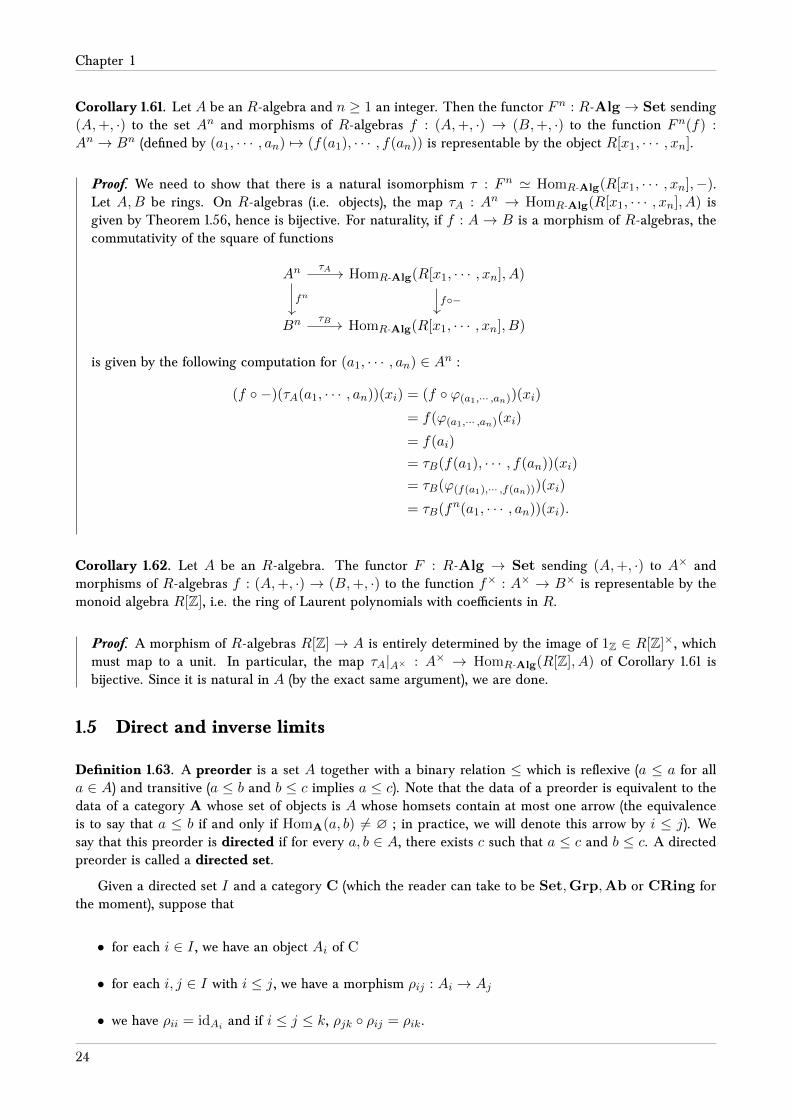
Corollary 1.61. Let A be an R-algebra and n ≥ 1 an integer. Then the functor Fn : R-Alg→ Set sending(A,+, ·) to the set An and morphisms of R-algebras f : (A,+, ·) → (B,+, ·) to the function Fn(f) :An → Bn (defined by (a1, · · · , an) 7→ (f(a1), · · · , f(an)) is representable by the object R[x1, · · · , xn].
Proof. We need to show that there is a natural isomorphism τ : Fn ' HomR-Alg(R[x1, · · · , xn],−).Let A,B be rings. On R-algebras (i.e. objects), the map τA : An → HomR-Alg(R[x1, · · · , xn], A) isgiven by Theorem 1.56, hence is bijective. For naturality, if f : A→ B is a morphism of R-algebras, thecommutativity of the square of functions
An HomR-Alg(R[x1, · · · , xn], A)
Bn HomR-Alg(R[x1, · · · , xn], B)
fn
τA
f−τB
is given by the following computation for (a1, · · · , an) ∈ An :
(f −)(τA(a1, · · · , an))(xi) = (f ϕ(a1,··· ,an))(xi)
= f(ϕ(a1,··· ,an)(xi)
= f(ai)
= τB(f(a1), · · · , f(an))(xi)
= τB(ϕ(f(a1),··· ,f(an)))(xi)
= τB(fn(a1, · · · , an))(xi).
Corollary 1.62. Let A be an R-algebra. The functor F : R-Alg → Set sending (A,+, ·) to A× andmorphisms of R-algebras f : (A,+, ·) → (B,+, ·) to the function f× : A× → B× is representable by themonoid algebra R[Z], i.e. the ring of Laurent polynomials with coefficients in R.
Proof. A morphism of R-algebras R[Z] → A is entirely determined by the image of 1Z ∈ R[Z]×, whichmust map to a unit. In particular, the map τA|A× : A× → HomR-Alg(R[Z], A) of Corollary 1.61 isbijective. Since it is natural in A (by the exact same argument), we are done.
1.5 Direct and inverse limits
Definition 1.63. A preorder is a set A together with a binary relation ≤ which is reflexive (a ≤ a for alla ∈ A) and transitive (a ≤ b and b ≤ c implies a ≤ c). Note that the data of a preorder is equivalent to thedata of a category A whose set of objects is A whose homsets contain at most one arrow (the equivalenceis to say that a ≤ b if and only if HomA(a, b) 6= ∅ ; in practice, we will denote this arrow by i ≤ j). Wesay that this preorder is directed if for every a, b ∈ A, there exists c such that a ≤ c and b ≤ c. A directedpreorder is called a directed set.
Given a directed set I and a category C (which the reader can take to be Set,Grp,Ab or CRing forthe moment), suppose that
• for each i ∈ I , we have an object Ai of C
• for each i, j ∈ I with i ≤ j, we have a morphism ρij : Ai → Aj
• we have ρii = idAi and if i ≤ j ≤ k, ρjk ρij = ρik.
24

Elementary properties of rings and their modules
An equivalent way to formulate the above is to suppose that we have a functor ρ : I → C, where ρ(i)def= Ai
and ρ(i ≤ j)def= ρij . Such a functor ρ is called a directed system (of sets, groups, abelian groups, rings,
etc.).
The inverse limitlim←−i∈I
Ai
is a limit of the functor ρ (by abuse of notation, since the morphisms ρij : Ai → Aj are often implicitlyunderstood, we omit them from the notation). More explicitly, this object is characterized up to a uniqueisomorphism by the following properties :
(i) For each j ∈ I , there is a morphism πj : lim←−i∈I Ai → Aj , called the projection to Aj
(ii) For each pair (j, k) ∈ I2 such that j ≤ k, the following diagram commutes :
lim←−i∈I
Ai
Aj Ak
πj πk
ρjk
(An object B paired with a collection of morphisms πBj j∈I satisfying (ii) is called a cone to ρ. Amorphism ρB,B′ : B → B′ between cones is said to commute with projections if it makes such acommutative diagram ; we also call such a morphism a morphism of cones to ρ.)
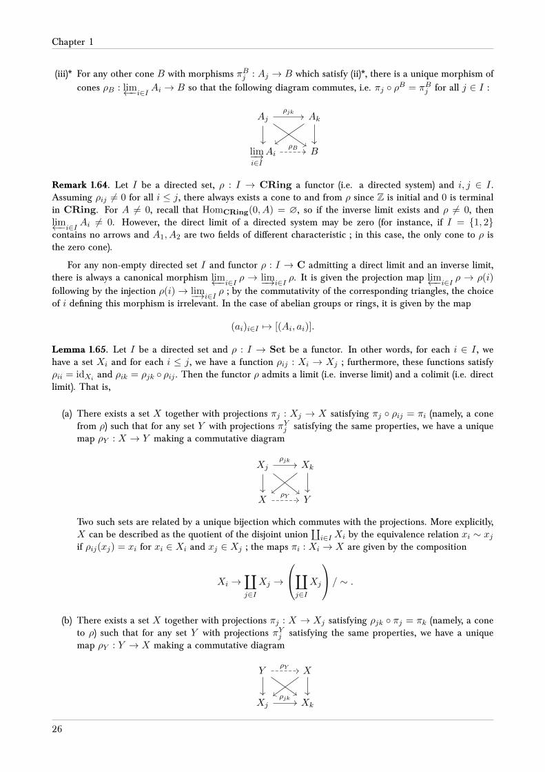
(iii) For any other cone B with morphisms πBj : B → Aj which satisfy property (ii) above, there is a uniquemorphism of cones ρB : B → lim←−i∈I Ai so that the following diagram commutes, i.e. πj ρB = πBjfor all j ∈ I :
B lim←−i∈I
Ai
Aj Ak
ρB
ρjk
The direct limitlim−→i∈I
Ai
is a colimit of the functor ρ (by abuse of notation, since the morphisms ρij : Ai → Aj are often implicitlyunderstood, we omit them from the notation). More explicitly, this object is characterized up to a uniqueisomorphism by the following properties :
(i)* For each j ∈ I , there is a morphism πj : Aj → lim−→i∈I Ai, called the projection from Aj
(ii)* For each pair (j, k) ∈ I2 such that j ≤ k, the following diagram commutes :
Aj Ak
lim−→i∈I
Ai
ρjk
πj πk
(An object B paired with a collection of morphisms πBj j∈I satisfying (ii) is called a cone from ρ.A morphism ρB,B′ : B → B′ between cones from ρ is said to commute with projections if it makessuch a commutative diagram ; we also call such a morphism a morphism of cones from ρ.)
25
Chapter 1
(iii)* For any other cone B with morphisms πBj : Aj → B which satisfy (ii)*, there is a unique morphism ofcones ρB : lim←−i∈I Ai → B so that the following diagram commutes, i.e. πj ρB = πBj for all j ∈ I :
Aj Ak
lim−→i∈I
Ai B
ρjk
ρB
Remark 1.64. Let I be a directed set, ρ : I → CRing a functor (i.e. a directed system) and i, j ∈ I .Assuming ρij 6= 0 for all i ≤ j, there always exists a cone to and from ρ since Z is initial and 0 is terminalin CRing. For A 6= 0, recall that HomCRing(0, A) = ∅, so if the inverse limit exists and ρ 6= 0, thenlim←−i∈I Ai 6= 0. However, the direct limit of a directed system may be zero (for instance, if I = 1, 2contains no arrows and A1, A2 are two fields of different characteristic ; in this case, the only cone to ρ isthe zero cone).
For any non-empty directed set I and functor ρ : I → C admitting a direct limit and an inverse limit,there is always a canonical morphism lim←−i∈I ρ → lim−→i∈I ρ. It is given the projection map lim←−i∈I ρ → ρ(i)
following by the injection ρ(i)→ lim−→i∈I ρ ; by the commutativity of the corresponding triangles, the choiceof i defining this morphism is irrelevant. In the case of abelian groups or rings, it is given by the map
(ai)i∈I 7→ [(Ai, ai)].
Lemma 1.65. Let I be a directed set and ρ : I → Set be a functor. In other words, for each i ∈ I , wehave a set Xi and for each i ≤ j, we have a function ρij : Xi → Xj ; furthermore, these functions satisfyρii = idXi and ρik = ρjk ρij . Then the functor ρ admits a limit (i.e. inverse limit) and a colimit (i.e. directlimit). That is,
(a) There exists a set X together with projections πj : Xj → X satisfying πj ρij = πi (namely, a conefrom ρ) such that for any set Y with projections πYj satisfying the same properties, we have a uniquemap ρY : X → Y making a commutative diagram
Xj Xk
X Y
ρjk
ρY
Two such sets are related by a unique bijection which commutes with the projections. More explicitly,X can be described as the quotient of the disjoint union
∐i∈I Xi by the equivalence relation xi ∼ xj
if ρij(xj) = xi for xi ∈ Xi and xj ∈ Xj ; the maps πi : Xi → X are given by the composition
Xi →∐j∈I
Xj →
∐j∈I
Xj
/ ∼ .
(b) There exists a set X together with projections πj : X → Xj satisfying ρjk πj = πk (namely, a coneto ρ) such that for any set Y with projections πYj satisfying the same properties, we have a uniquemap ρY : Y → X making a commutative diagram
Y X
Xj Xk
ρY
ρjk
26

Elementary properties of rings and their modules
Two such sets are related by a unique bijection which commutes with the projections. In categoricallanguage, an instance of this set is given by the set Cone(∗, ρ) of cones from the one-point set ∗ toρ. More explicitly, Cone(∗, ρ) ⊆
∏i∈I Xi can be described as the set of functions f : I →
∐i∈I Xi
such that ρij(f(i)) = f(j) for all i ≤ j ; the I-indexed sequence (xi)i∈I (where f ∈ Cone(∗, ρ)
and xidef= f(i)) is called a coherent sequence, so that Cone(∗, ρ) corresponds to the set of all
coherent sequences in∏i∈I Xi.
Proof. (a) The collection of maps πYi : Xi → Y gives rise to a map∐i∈I Xi → Y , and since Y satisfies
(ii)* in Definition 1.63, we can mod out the equivalence relation to obtain a map ρY : X → Yuniquely determined by the required restrictions. The rest is obvious.
(b) The set Cone(∗, ρ) is well-defined ; the projections πj : Cone(∗, ρ) → Xj are given byrestricting those of
∏i∈I Xi to Cone(∗, ρ) ; by definition of Cone(∗, ρ), we have ρij πj = πi
since πi(f) = f(i) for f ∈ Cone(∗, ρ). Given a set Y with the properties mentioned above,an element y ∈ Y gives rise to a function fy : I →
∐i∈I Xi defined by fy(i) = πYi (y) and by
Definition 1.63, property (ii) of Y , we have fy ∈ Cone(∗, ρ). The association y 7→ fy definesthe unique map ρY : Y → X since the commutativity of the diagram forces fy(i) = πYi (y). Theunicity of X is given by the standard proof using the universal property and is omitted.
Theorem 1.66. Let I be a directed system and ρ : I → C a directed system in C where C = Ab or
C = CRing. Write ρ(i)def= Ai.
(a) The direct limit lim−→i∈I Ai exists in the category C. Its elements can be described as equivalenceclasses of pairs [(Ai, xi)] where xi ∈ Ai and two pairs (Ai, xi) ∼ (Aj , xj) are equivalent if thereexists k ≥ i, j such that ρik(xi) = ρjk(xj). To add (resp. multiply) two equivalence classes [(Ai, xi)]and [(Aj , xj)], find k ≥ i, j so that addition (resp. multiplication) is given by
[(Ai, xi)] + [(Aj , xj)]def= [(Ak, ρik(xi) + ρjk(xj)]
(replace + by juxtaposition to define multiplication).
(b) The inverse limit lim←−i∈I Ai exists in the category C. As a set, it equals the inverse limit of theinverse system of sets given by ρ. Therefore, its elements can be described as coherent sequences(xi)i∈I ∈
∏i∈I Ai where xi ∈ Ai and if i ≤ j, ρij(xi) = xj . Addition (and multiplication if
C = CRing) is performed pointwise. (If C = CRing, the unit element of lim←−i∈I Ai is the coherentsequence (1Ai)i∈I .)
Proof. (a) If C = Ab, it is not hard to check that repeating the construction of Lemma 1.65 works aslong as we use the appropriate coproduct, i.e. the direct sum. The subgroup H generated by theelements xi − xj ∈
⊕k∈I Ak (where i, j ≤ k, xi ∈ Ai, xj ∈ Aj and ρik(xi) = ρjk(xj)) is used
to form the quotient lim←−i∈I Aidef=(⊕
i∈I Ai)/H . That it is an abelian group is immediate. Note
that “(Ai, xi) ∼ (Aj , xj) if and only if ρik(xi) = ρjk(xj) for some k ≥ i, j” is immediately seen tobe an equivalence relation. Given
(∑∗i∈I xi
)+ H , let i1, · · · , in ∈ I be the indices where xi 6= 0.
Then there exists k ≥ i1, · · · , in since I is directed, and thus( ∗∑i∈I
xi
)+H =
n∑j=1
ρijk(xij )︸ ︷︷ ︸∈Ak
+H.
This gives existence of the representation as an equivalence class of pairs (Ai, xi).
27

Chapter 1
If C = CRing, because a directed system of rings is in particular a directed system of abeliangroups, we can form the abelian group
(⊕i∈I Ai
)/H as before. We define multiplication as in
the statement. Given xi ∈ Ai, xj ∈ Aj and xk ∈ Ak, find ` ∈ I such that i, j, k ≤ `. Theassociativity, distributivity and commutativity of multiplication then amounts to the fact that itholds in A` since we can replace xi by ρi`(xi), xj by ρj`(xj) and xk by ρk`(xk). If I is empty,then lim←−i∈I Ai = Z since Z is initial in CRing. Otherwise, pick i ∈ I and consider 1Ai + H . Ifj ≤ i, note that ρji(1Aj ) = 1Ai ; if i ≤ j, note that ρij(1Ai) = 1Aj . Since I is directed, this means1Ai +H = 1Aj +H for all i, j ∈ I , therefore 1Ai +H is a unit element for this ring.
By the previous paragraph, if Y is a cone from ρ, there is a unique morphism of abelian groupsρY : lim−→i∈I Ai → Y , so it suffices to show that it is a morphism of rings, i.e. that it respects
multiplication. The morphism is given by ρY (xi+H)def= πYi (xi), hence since the πYi are morphisms
of rings, given xi ∈ Ai and xj ∈ Aj , fixing k ≥ i, j, we have
ρY ((xi +H)(xj +H)) = ρY (ρik(xi)ρjk(xj) +H)
= πYk (ρik(xi)ρjk(xj))
= πYk (ρik(xi))πYk (ρjk(xj))
= πYi (xi)πYj (xj)
= ρY (xi +H)ρY (xj +H).
(Note that although not every element of lim−→i∈I Ai can be written as xi + H for some xi ∈ Ai,since ρY respects addition, we can check that an equation for ρY holds by restricting to this case.)
(b) By Lemma 1.65, since∏i∈I Ai admits a canonical structure of an object in C (i.e. abelian
group or ring) which makes the projections πj :∏i∈I Ai → Aj morphisms in C, we can en-
dow Cone(∗, ρ) ⊆∏i∈I Ai with a subobject structure (namely subgroup or subring) and restrict
the morphisms to it. By the universal property of the product in C, we are done.
Example 1.67. (i) Let I be a directed system such that there exists i ∈ I with the property that forall j ∈ I , i ≥ j (in other words, i is a maximum in I ). Then lim←−j∈I Aj = Ai. (We will non-trivial examples of inverse limits when we will discuss completions of a ring with respect to an ideal.)Similarly, if there exists i ∈ I such that for all j ∈ I , i ≤ j, then lim−→j∈J Aj = Ai.
(ii) Suppose ρ : I → Set is a functor such that Xidef= ρ(i) ⊆ X and ρij : Xi → Xj is the inclusion map
for each i ≤ j. Thenlim−→i∈I
Xi =⋃i∈I
Xi, lim←−i∈I
Xi =⋂i∈I
Xi.
This is easy to see via the universal property : the universal property of the direct limit can betranslated to “every collection of functions on the Xi which agree on overlaps can be extended to theunion” and the universal property of the inverse limit says “any collection of functions to X whichmaps inside each Xi maps into the intersection”. This argument can be repeated if ρ maps into Ab orCRing and the inclusion Xi ⊆ X is an inclusion of abelian groups or rings, and the result remainsthe same.
(iii) Let I be a directed system of rings and assume that for each i ≤ j, ρij is an inclusion map Ai ⊆ Aj .Then lim−→i∈I Ai '
⋃i∈I Ai is a ring. We can obviously turn the union into a ring by letting xi + xj
be added in a common subring Ak with Ai, Aj ⊆ Ak and similarly for multiplication ; note that0, 1 ∈
⋂i∈I Ai. The isomorphism
⋃i∈I Ai → lim−→i∈I Ai is given by sending x ∈ Ai to [(Ai, x)] ; the
choice of ring Ai is irrelevant since if x ∈ Ai ∩ Aj , then [(Ai, x)] = [(Ak, x)] = [(Aj , x)] wheneverk ≥ i, j. This obviously respects addition, multiplication and is bijective, so we are done.
28

Elementary properties of rings and their modules
For those who know some field theory, this is useful to build a field out of a tower of fields : givena directed system of fields indexed by N, we have inclusions F0 ⊆ F1 ⊆ · · · and we can define
Fdef=⋃i∈I Fi. Because we have described the union as a direct limit, we now know that it satisfies
the universal property of the direct limit.
29

Chapter 2
Operations on ideals
2.1 Intersections, sums and products
Proposition 2.1. Let a, b E A be ideals. Then a ∩ b is an ideal. More generally, the intersection⋂i∈I ai of
any family of ideals aii∈I of A is an ideal of A.
Proof. This follows straightforwardly from Lemma 1.20 (ii).
Proposition 2.2. Let aii∈Z be a sequence of ideals of a ring A such that ai ⊆ ai+1 for all i ∈ Z. Thenthe subset
⋃i∈Z
ai is an ideal of A. Note that as a direct corollary, the index set Z can be replaced by any
subset of the form n ∈ Z | n ≥ n0, such as N (this follows by setting ai = 0 for i < n0).
Proof. If b1, b2 ∈⋃i∈Z ai and a ∈ A, then there exists ai1 3 b1 and ai2 3 b2, so that b1, b2 ∈ amaxi1,i2.
In particular, b1 + b2, ab1 ∈ amaxi1,i2 ⊆⋃i∈Z ai.
Lemma 2.3. Suppose a, b E A are ideals and a = (S)A. Then a ⊆ b if and only if S ⊆ b.
Proof. On one hand, we have S ⊆ a, hence a ⊆ b implies S ⊆ a ⊆ b. On the other hand, Lemma 1.20(ii) tells us that if we have a =
∑∗i∈I aisi ∈ a with ai ∈ A, si ∈ S ⊆ b, then a ∈ b.
Definition 2.4. Let A be a ring and a, b E A. Define
a + bdef= x+ y | x ∈ a, y ∈ b,
called the sum of a and b. More generally, if aii∈I is a family of ideals of A, define
∑i∈I
aidef=
(⋃i∈I
ai
)A
=
∗∑i∈I
xi
∣∣∣∣∣ xi ∈ ai
.
Proposition 2.5. Let A be a ring and aii∈I be a family of ideals in A. Then∑
i∈I ai is the smallest idealcontaining all of the ai’s, i.e. ∑
i∈Iai =
⋂cEAai⊆c
c.
30

Elementary properties of rings and their modules
Proof. (⊆) Assume ai ⊆ c for all i ∈ I . Since⋃i∈I ai ⊆ c, we have
∑i∈I ai ⊆ c by Lemma 2.3. (Using
the alternate description of∑
i∈I ai, this also follows from Lemma 1.20.)
(⊇) It suffices to see that adef=∑
i∈I ai is an ideal since it obviously contains all of the ai ; for this, we useLemma 1.20 (ii). The sum
∑∗i∈I xi +
∑∗i∈I yi where xi, yi ∈ ai belongs to a since xi + yi ∈ ai. If c ∈ A,
then c∑∗
i∈I xi =∑∗
i∈I cxi also belongs to a since each cxi belongs again to ai.
Definition 2.6. Let A be a ring and a, b E A. Define the product of two ideals as
abdef=
∗∑i∈I
aibi
∣∣∣∣∣ ai ∈ a, bi ∈ b
.
More generally, if a1, · · · , am E A, define the product of n ideals as
m∏j=1
aj = a1 · . . . · amdef=
∗∑i∈I
m∏j=1
aij
∣∣∣∣∣∣ aij ∈ aj for j = 1, · · · ,m
.
As a particular case, if a1 = · · · = am, we define inductively a0 = A and am = a · . . . · a︸ ︷︷ ︸m times
.
If Sii∈I is a family of subsets of A, define
m∏i=1
Sidef=
m∏i=1
ai
∣∣∣∣∣ ai ∈ Si, i = 1, · · · ,m
.
Proposition 2.7. Let A be a ring and aii∈I a family of ideals. If ai = (Si)A for subsets Si ⊆ ai, then
m∏i=1
ai =
(m∏i=1
Si
)A
.
Proof. The inclusion (⊇) is obvious. For (⊆), let aj ∈ aj = (Sj)A, j = 1, · · · ,m. Then there exists sumsof the form
aj =∗∑i∈I
aijsij , sij ∈ Si, aij ∈ A.
It follows that∏mj=1 ai is a sum of terms of the form s1 · · · sm multiplied by elements of A, where sj ∈ S,
j = 1, · · · ,m. This proves∏mj=1 aj ∈
(∏mj=1 Sj
)A. Since the latter is an ideal, sums of such elements of∏m
j=1 aj are in(∏m
j=1 Sj
)A, so we are done.
Remark 2.8. If a, b E A are ideals, the products ab as ideals and as sets don’t agree in general, butProposition 2.7 such that the ideal generated by both products are equal. We therefore do not distinguishsince we will never take products of ideals considered as sets, unless explicitly mentioned.
Proposition 2.9. The operations ∩, + and · are commutative and associative on ideals. Furthermore, forany a, b, c E A, we have
a(b + c) = ab + ac, ab ⊆ a ∩ b.
Proof. In all cases, commutativity and associativity are obvious ; it is trivial for ∩ and follows fromassociativity of addition and multiplication of elements in the ring for + and ·. Suppose a = (Sa)A,b = (Sb)A and c = (Sc)A. Then
a(b + c) = (Sa(Sb ∪ Sc))A = (SaSb ∪ SaSc)A = (SaSb)A + (SaSc)A = ab + ac.
31

Chapter 2
Note that Sa(Sb ∪ Sc) = SaSb ∪ SaSc holds by definition of the product of sets, c.f. Definition 2.6.Since Sa ⊆ a, we have SaSb ⊆ a ; similarly, SaSb ⊆ b, hence SaSb ⊆ a ∩ b. The inclusion follows byLemma 2.3.
Corollary 2.10. Let a, b E A be proper ideals. Then ab E A is a proper ideal.
Proof. We have ab ⊆ a ∩ b ⊆ a ( A.
Remark 2.11. The inclusion ab ⊆ a ∩ b is not an equality in general. For instance, if p ∈ Z is greater than1, then
(pZ)2 = p2Z ( pZ = pZ∩pZ .The equality fails more generally in any integral domain with an ideal a satisfying a2 6= a ; this is the caseof principal ideals a = (a)A where a ∈ A \ (0 ∪A×) since a2 = (a2) and a 6= ca2 unless ac = 1, i.e. a isa unit.
We will prove later that if a = nZ and b = mZ are two non-zero proper ideals in the ring Z, thenab = a ∩ b if and only if the greatest common divisor (n,m) equals 1, i.e. if and only if a + b = Z ; c.f.Theorem 2.17.
2.2 The Chinese Remainder Theorem
Definition 2.12. Let a, b E A be two distinct proper ideals. The pair a, b is said to be comaximal ifa + b = A ; in this case, we also say that a and b are comaximal. More generally, the family aii∈I ofdistinct proper ideals is called pairwise comaximal if for every i, j ∈ I with i 6= j, the pair ai, aj iscomaximal.
Lemma 2.13. Let a, b E A. If a and b are comaximal, then ab = a ∩ b.
Proof. By Proposition 2.9, we have
a ∩ b = (a ∩ b)(a + b) = (a ∩ b)a + (a ∩ b)b ⊆ ab ⊆ a ∩ b.
Lemma 2.14. If a, b1 and a, b2 are comaximal, then a, b1b2 is comaximal.
Proof. There exists a1 ∈ a, b1 ∈ b1 such that a1 + b1 = 1, and there exists a2 ∈ a, b2 ∈ b2 such thata2 + b2 = 1. Therefore, with
adef= a1 + a2 − a1a2 ∈ a,
we haveb1b2 = (1− a1)(1− a2) = 1− a.
This means a+ b1b2 = 1, i.e. a and b1b2 are comaximal because a + b1b2 3 1.
Definition 2.15. Let A1, · · · , An be rings and define
Adef= A1 × · · · ×An =
n∏i=1
Aidef= (a1, · · · , an) | ai ∈ Ai.
Then (A,+, ·) where the operations are taken component-wise, is a ring where 1A = (1A1 , · · · , 1An). (Inparticular, if I is finite, then AI = A× · · · ×A︸ ︷︷ ︸
n times
; c.f. Example 1.5.)
32

Elementary properties of rings and their modules
Remark 2.16. The mapπj : A→ Aj
(a1, . . . , an) 7→ aj
is a morphism, butιj : Aj → A
aj 7→ (0, . . . , 0, aj , 0, . . . , 0)
is not a morphism in this case, because ιj(1) 6= 1 (this is the only missing property ; therefore the ιj aremorphisms of non-commutative rings).
Theorem 2.17. (Chinese Remainder Theorem) For a ring A and ideals a1, . . . , an ⊆ A, define the morphism
ϕ : A→n∏i=1
A/ai
a 7→ ϕ(a)def= (a+ ai)1≤i≤n.
(a) If (a1, · · · , an) are pairwise comaximal, then∏ni=1 ai =
⋂ni=1 ai.
(b) ϕ is surjective if and only if a1, · · · , an are pairwise comaximal.
(c) The map ϕ satisfies kerϕ =⋂ni=1 ai. Therefore, if a1, · · · , an are pairwise comaximal, we have a
canonical isomorphism
A
/n∏i=1
ai 'n∏i=1
A/ai.
Proof. (a) By induction on n. Lemma 2.13 proves the case n = 2 and the case n = 1 is trivial. Assumen > 2. By Lemma 2.14, we can prove that for 1 ≤ i < n − 1, since (ai, an−1) and (ai, an) arecomaximal, so is (ai, an−1an) ; since (an−1, an) are comaximal, an−1 ∩ an = an−1an. Using theinduction hypothesis, since (a1, · · · , an−2, an−1an) are pairwise comaximal,
n⋂i=1
ai =
(n−2⋂i=1
ai
)∩ an−1an =
(n−2∏i=1
ai
)· an−1an =
n∏i=1
ai.
(b) (⇒) If ϕ is surjective, then in particular, for each 1 ≤ i < j ≤ n, there is a solution to the system
x ≡ 0 (mod ai), x ≡ 1 (mod aj).
This means that x ∈ ai and ydef= 1− x ∈ aj are such that 1 = x+ y ∈ ai + aj , so the pair (ai, aj)
is comaximal.
(⇐) If a1 is comaximal to a2, . . . , an, then it is comaximal to bdef= a2 . . . an =
⋂ni=2 ai by Lemma
1.4 applied inductively and by (a). Therefore there exists x1 ∈ a1 and y1 ∈ b such that x1 + y1 = 1.In particular, ϕ(y1) = (1 + a1, 0 + a2, . . . , 0 + an). Substituting the role of a1 by ai and letting
πi :
n∏i=1
A/ai → A/ai
denote the projections, we get yi ∈ A such that πi(ϕ(yi)) = 1+ai and πj(ϕ(yi)) = 0+aj for j 6= i.Let (a1, · · · , an) ∈ An. If we want y ∈ A with ϕ(y) = (a1 + a1, · · · , an + an), take y =
∑ni=1 aiyi.
It follows that
πi(ϕ(y)) =n∑i=1
πi(ϕ(ai))πi(ϕ(yi)) = ai + ai =⇒ ϕ(y) = (a1 + a1, · · · , an + an).
Therefore ϕ is surjective.
33
Chapter 2
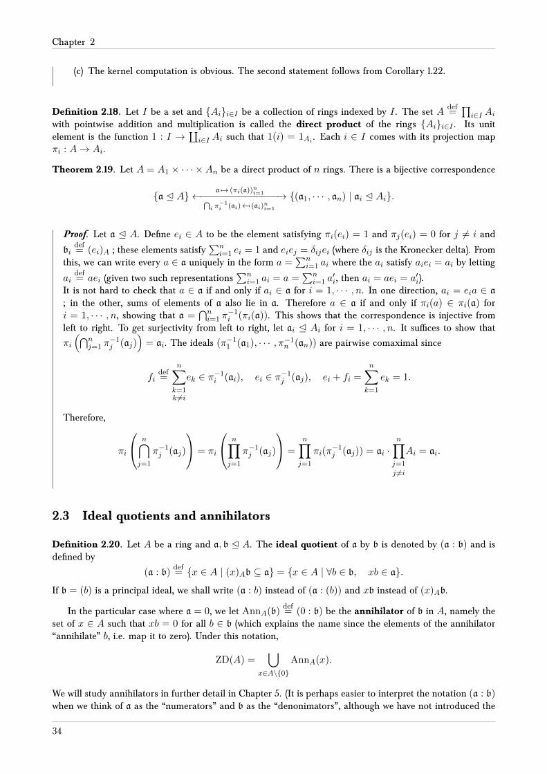
(c) The kernel computation is obvious. The second statement follows from Corollary 1.22.
Definition 2.18. Let I be a set and Aii∈I be a collection of rings indexed by I . The set Adef=∏i∈I Ai
with pointwise addition and multiplication is called the direct product of the rings Aii∈I . Its unitelement is the function 1 : I →
∐i∈I Ai such that 1(i) = 1Ai . Each i ∈ I comes with its projection map
πi : A→ Ai.
Theorem 2.19. Let A = A1 × · · · ×An be a direct product of n rings. There is a bijective correspondence
a E Aa 7→ (πi(a))ni=1←−−−−−−−−−−−−−−→⋂
i π−1i (ai)← [ (ai)ni=1
(a1, · · · , an) | ai E Ai.
Proof. Let a E A. Define ei ∈ A to be the element satisfying πi(ei) = 1 and πj(ei) = 0 for j 6= i and
bidef= (ei)A ; these elements satisfy
∑ni=1 ei = 1 and eiej = δijei (where δij is the Kronecker delta). From
this, we can write every a ∈ a uniquely in the form a =∑n
i=1 ai where the ai satisfy aiei = ai by letting
aidef= aei (given two such representations
∑ni=1 ai = a =
∑ni=1 a
′i, then ai = aei = a′i).
It is not hard to check that a ∈ a if and only if ai ∈ a for i = 1, · · · , n. In one direction, ai = eia ∈ a; in the other, sums of elements of a also lie in a. Therefore a ∈ a if and only if πi(a) ∈ πi(a) fori = 1, · · · , n, showing that a =
⋂ni=1 π
−1i (πi(a)). This shows that the correspondence is injective from
left to right. To get surjectivity from left to right, let ai E Ai for i = 1, · · · , n. It suffices to show that
πi
(⋂nj=1 π
−1j (aj)
)= ai. The ideals (π−1
1 (a1), · · · , π−1n (an)) are pairwise comaximal since
fidef=
n∑k=1k 6=i
ek ∈ π−1i (ai), ei ∈ π−1
j (aj), ei + fi =n∑k=1
ek = 1.
Therefore,
πi
n⋂j=1
π−1j (aj)
= πi
n∏j=1
π−1j (aj)
=
n∏j=1
πi(π−1j (aj)) = ai ·
n∏j=1
j 6=i
Ai = ai.
2.3 Ideal quotients and annihilators
Definition 2.20. Let A be a ring and a, b E A. The ideal quotient of a by b is denoted by (a : b) and isdefined by
(a : b)def= x ∈ A | (x)Ab ⊆ a = x ∈ A | ∀b ∈ b, xb ∈ a.
If b = (b) is a principal ideal, we shall write (a : b) instead of (a : (b)) and xb instead of (x)Ab.
In the particular case where a = 0, we let AnnA(b)def= (0 : b) be the annihilator of b in A, namely the
set of x ∈ A such that xb = 0 for all b ∈ b (which explains the name since the elements of the annihilator“annihilate” b, i.e. map it to zero). Under this notation,
ZD(A) =⋃
x∈A\0
AnnA(x).
We will study annihilators in further detail in Chapter 5. (It is perhaps easier to interpret the notation (a : b)when we think of a as the “numerators” and b as the “denonimators”, although we have not introduced the
34

Elementary properties of rings and their modules
notion of fractions yet, which will come with localization in Chapter 8 ; this interpretation is correct in somecases such as unique factorization domains when b ⊆ a and so is worth having in mind.)
Example 2.21. If A = Z, a = (m) and b = (n) for m,n > 0, write m =∏ki=1 p
aii and n =
∏ki=1 p
bii (the
case ai or bi equal to zero is added, we just wanted all the primes involved in the factorization of both ; note
that the p1, · · · , pk are distinct). Let cidef= maxai − bi, 0. Then
(a : b) = (q), qdef=
k∏i=1
pcii .
To see this, suppose that x ∈ N+ is such that xb ⊆ a, i.e. m divides xn. Write x = s∏ki=1 p
dii where s
and pi are coprime for i = 1, · · · , k. From elementary number theory, we know that we can assume withoutloss of generality that s = 1. The fact that m divides xn is equivalent to bi + di ≥ ai, i.e. di ≥ ai − bi.Therefore, the minimal possible value of di is ci (because di ≥ 0 by assumption), i.e. x ∈ (a : b) if and onlyif x ∈ (q).
Proposition 2.22. Let A be a ring and a, b, c E A.
(a) We have a ⊆ (a : b).
(b) We have (a : b)b ⊆ a.
(c) We have ((a : b) : c) = (a : bc) = ((a : c) : b).
(d) For any family of ideals aii∈I , we have(⋂
i∈I ai : b)
=⋂i∈I(ai : b).
(e) For any family of ideals bii∈I , we have(a :∑
i∈I bi)
=⋂i∈I(a : bi).
Proof. (a) This follows from ab ⊆ a ∩ b ⊆ a.
(b) Since (a : b)b is generated by products xb where x ∈ (a : b) and b ∈ b, by definition, xb ∈ a, thusthe result.
(c) We only need to prove the first equality since the product of ideals is a commutative operation.
(⊆) If x ∈ ((a : b) : c), this means xc ⊆ (a : b), e.g. for any y ∈ c, xyb ⊆ a. Thereforexcb = xbc ⊆ a, which means x ∈ (a : bc).
(⊇) If x ∈ (a : bc), y ∈ b and z ∈ c, we have xyz ∈ a, which shows that xy ∈ (a : b), i.e.xc ⊆ (a : b), so x ∈ ((a : b) : c).
(d) The inclusion xb ⊆⋂i∈I ai is equivalent to xb ⊆ ai for all i ∈ I , i.e. x ∈
⋂i∈I(ai : b).
(e) The inclusion x(∑
i∈I bi)⊆ a is equivalent to xbi ⊆ a for all i ∈ I , i.e. x ∈
⋂i∈I(a : bi).
35

Chapter 3
Prime, maximal and radical ideals
3.1 Prime ideals
Let A be a ring. Recall that A is called an integral domain if NZD(A) = A\0 ; if A 6= 0, this is equivalentto ZD(A) = 0. Another way to phrase this is that a ring A 6= 0 is an integral domain if the product ofnon-zero elements remains non-zero.
Definition 3.1. A subset S ⊆ A is called multiplicative if 1 ∈ S and
x, y ∈ S =⇒ xy ∈ S.
Equivalently, a subset S ⊆ A is multiplicative if (S, ·) is a submonoid of (A, ·).
Lemma 3.2. Let ϕ : A→ B be a morphism.
(a) If S ⊆ A is multiplicative, then ϕ(S) is multiplicative.
(b) If T ⊆ B is multiplicative, then ϕ−1(T ) is multiplicative.
Proof. For (a), if t1, t2 ∈ ϕ(S), write ϕ(s1) = t1 and ϕ(s2) = t2 so that ϕ(s1s2) = t1t2 ∈ ϕ(S) ; clearly1B = ϕ(1A) ∈ ϕ(S). For (b), if s1, s2 ∈ ϕ−1(T ), then ϕ(s1s2) = ϕ(s1)ϕ(s2) ∈ T , hence s1s2 ∈ ϕ−1(T ),and again 1A ∈ ϕ−1(T ) since ϕ(1A) = 1B ∈ T .For those who know about monoids, this is a simple consequence about the fact that the image (resp.inverse image) of a submonoid under a morphism of monoids is a monoid (which is essentially what wejust proved above).
Theorem 3.3. Let p E A. The following are equivalent :
(i) A/p is an integral domain
(ii) p 6= A and
x, y ∈ A, xy ∈ p =⇒ x ∈ p or y ∈ p
(iii) p 6= A and
a, b E A, ab ⊆ p =⇒ a ⊆ p or b ⊆ p
(iv) The set A \ p is multiplicative.
36

Elementary properties of rings and their modules
Proof. ( (i) ⇐⇒ (iv) ) For a, b ∈ A \ p, property (i) says that (a + p)(b + p) 6= (0 + p) and property (iv)says that ab ∈ A \ p ; the two are clearly equivalent.( (ii) ⇒ (iii) ) Suppose a, b 6⊆ p. Then there exists x ∈ a \ p and y ∈ b \ p, but xy ∈ ab ⊆ p. It follows by(ii) that x ∈ p or y ∈ p, a contradiction.( (iii) ⇒ (ii) ) Given x, y ∈ A with xy ∈ p, let a = (x) and b = (y), so that ab ⊆ p. It follows that a ⊆ por b ⊆ p, hence x ∈ p or y ∈ p.( (ii) ⇐⇒ (iv) ) First, note that the three statements p 6= A, 1 /∈ p and 1 ∈ A \ p are equivalent. Second,[
a, b ∈ A, ab ∈ p =⇒ a ∈ p or b ∈ p]⇐⇒
[a, b ∈ A \ p =⇒ ab ∈ A \ p
].
Definition 3.4. An ideal p E A satisfying any of the conditions of Theorem 3.3 is called a prime ideal.Define
Spec (A)def= p E A | p is prime ⊆ Ideal (A) ,
which we call the prime spectrum of A.
Proposition 3.5. Let ϕ : A→ B be a morphism.
(i) If q ∈ Spec (B), then ϕ−1(q) ∈ Spec (A).
(ii) If ϕ is surjective and p ∈ Spec (A) satisfies kerϕ ⊆ p, then ϕ(p) ∈ Spec (B).
Proof. (i) There are many proofs for this.
• With elements : if a, b ∈ A satisfy ab ∈ ϕ−1(q), then ϕ(a)ϕ(b) = ϕ(ab) ∈ q, so ϕ(a) ∈ q orϕ(b) ∈ q, that is, a ∈ q or b ∈ q.
• With quotient rings : consider the following commutative diagram :
A B
A/ϕ−1(q) B/q
ϕ
πϕ−1(q) πq
ϕ
The map ϕ is obtained by the universal property for quotient rings, c.f. Theorem 1.21. Ifa, b ∈ A/ϕ−1(q) are non-zero, then ϕ(ab) = ϕ(a)ϕ(b) 6= 0 since B/q is an integral domainand ϕ(a), ϕ(b) 6= 0. Therefore ab 6= 0, i.e. A/ϕ−1(q) is an integral domain.
• With multiplicative subsets : Note that A \ ϕ−1(q) = ϕ−1(A \ q). The result follows fromLemma 3.2.
(ii) Again, there are many proofs for this. In every case, note that ϕ(p) E B by Theorem 1.26.
• With elements : assume b1, b2 ∈ B satisfy b1b2 ∈ ϕ(p). Since ϕ is surjective, we can finda1, a2 ∈ p with ϕ(ai) = bi, i = 1, 2. Now ϕ(a1a2) = ϕ(a1)ϕ(a2) ∈ ϕ(p), so choose p ∈ psuch that ϕ(a1a2) = ϕ(p). It follows that a1a2 − p ∈ kerϕ ⊆ p, e.g. a1a2 ∈ p. Thereforea1 ∈ p or a2 ∈ p, e.g. b1 ∈ ϕ(p) or b2 ∈ ϕ(p).
• With quotients : the morphism A→ B → B/ϕ(p) is surjective with kernel
ϕ−1(ϕ(p)) + kerϕ = p + kerϕ = p,
so B/ϕ(p) ' A/p is an integral domain.
• With multiplicative subsets : since A \ p is multiplicative, so is ϕ(A \ p) by Lemma 3.2. Sincekerϕ ⊆ p, we must have ϕ(p)∩ϕ(A/p) = ∅ because if p ∈ p, s ∈ A \ p satisfy ϕ(p) = ϕ(s),then p− s ∈ kerϕ ⊆ p, hence s ∈ p, a contradiction. We deduce that
B \ ϕ(p) = ϕ(A) \ ϕ(p) = ϕ(A \ p),
37

Chapter 3
hence ϕ(p) ∈ Spec (B) is a prime ideal.
Corollary 3.6. Let A be a ring and a E A an ideal. Theorem 1.26 restricts to a bijective correspondencebetween prime ideals in Spec (A) containing a and prime ideals in Spec (A/a).
Proof. This is clear since the correspondence is a bijection which maps prime ideals to prime ideals inboth directions by Proposition 3.5.
Definition 3.7. The set of ideals a E A | a 6= A can be partially ordered under inclusion ; we say thata ≤ b if a ⊆ b. This partially ordered set is denoted by Ideal (A). It will be of interest to study the minimaland maximal elements of Ideal (A).
Theorem 3.8. Let m E A. The following are equivalent :
(i) A/m is a field
(ii) If x ∈ A \m, there exists y ∈ A \m such that xy ≡ 1 (mod m)
(iii) If a E A and m ⊆ a ⊆ A, then a = m or a = A
(iv) The ideal m is a maximal element in Ideal (A).
Proof. ( (i) ⇐⇒ (ii) ) The element x + m ∈ A/m is invertible if and only if there exists y ∈ A with(x+m)(y+m) = (1+m), i.e. xy ≡ 1 (mod m). Conversely, xy ≡ 1 (mod m) implies (x+m)(y+m) =(1 + m).( (ii)⇒ (iii) ) Assume m ( a ⊆ A and pick x ∈ a \m ⊆ A \m. Then xy ≡ 1 (mod m) means there existsm ∈ m ⊆ a such that 1 = xy −m ∈ a, so a = A.( (iii) ⇐⇒ (iv) ) By definition of maximality, we can re-write (iv) as “if m ⊆ a ( A, then m = a”, which isequivalent to (iii).( (iii),(iv) ⇒ (i) ) The fact that the bijection of Theorem 1.26 is inclusion-preserving means it is anisomorphism of partially ordered sets. This means the ideal (0) is a maximal element in Ideal (A/m),i.e. satisfies (iii). Therefore, if a + m ∈ A/m \ 0, (a)A/m = A/m, hence a is invertible, so A/m is afield.
3.2 Maximal ideals and vanishing loci
Definition 3.9. An ideal m E A satisfying any of the properties of Theorem 3.8 is called a maximal ideal.The subset
MaxSpec (A)def= m E A | m ∈ Ideal (A) is maximal
is called the maximal spectrum of A.
Example 3.10. • Spec (Z) = (0) ∪ (p) | p is a prime number . This is because Z is an integraldomain and for n > 0, nZ is prime if and only if n is a prime number (c.f. Corollary 1.41). By thesame corollary, MaxSpec (Z) = (p) | p is a prime number .
• The spectrum of a field K is a point : Spec (K) = (0). This follows from Proposition 1.44.
• Maximal ideals are prime ideals, for if m is maximal, then A/m is a field, hence an integral domain.This gives the inclusion MaxSpec (A) ⊆ Spec (A).
Theorem 3.11. Let S ⊆ A be a multiplicative subset and a E A such that a ∩ S = ∅, or equivalently,
a ⊆ A \ S. The subset Φa,Sdef= b ∈ Ideal (A) | a ⊆ b ⊆ A \ S admits a maximal element with respect to
inclusion. Furthermore, every such maximal element is a prime ideal.
38

Elementary properties of rings and their modules
Proof. We simply apply Zorn’s lemma on the partially ordered set Φa,S . Note that a ∈ Φa,S 6= ∅. Givena chain
b1 ⊆ b2 ⊆ · · · ⊆ bn ⊆ · · ·
of ideals in Φa,S , then⋃n≥1 bn is an ideal by Proposition 2.2 and since all bn satisfy a ⊆ bn ⊆ A \S, we
have a ⊆⋃n≥1 bn ⊆ A \ S.
Let p be a maximal element in Φa,S , and assume we have a1, a2 ∈ A \ p with a1a2 ∈ p. Defineai = p + (ai) for i = 1, 2. By assumption a ⊆ p ( ai, and by maximality of p, we must have ai 6⊆ A \ S,i.e. ai ∩ S 6= ∅. Therefore there is an element si ∈ ai ∩ S for i = 1, 2, and since S is multiplicative,s1s2 ∈ S. Since si ∈ ai = p + (ai), we can write si = pi + yiai for some pi ∈ p and yi ∈ A, so that
s1s2 = (p1 + y1a1)(p2 + y2a2) = p1(p2 + y2a2) + p2(y1a1) + (y1a1)(y2a2)︸ ︷︷ ︸a1a2∈p
∈ p,
hence s1s2 ∈ p ∩ S = ∅, a contradiction.
Corollary 3.12. (Krull’s theorem) Every proper ideal a E A is contained in a maximal ideal.
Proof. Use Theorem 3.11 with S = 1. Then it follows that intersecting S is equivalent to being a properideal, so maximal elements in Φa,S become maximal ideals.
Corollary 3.13. Let A be a ring. Then Spec (A) = ∅ if and only if A = 0.
Proof. Clearly A = 0 implies Spec (A) = ∅ since 0 admits no proper ideals. If A 6= 0, then by Krull’stheorem A admits a maximal ideal, which is prime.
Corollary 3.14. If A is a ring, then
A× = A \
⋃m∈MaxSpec(A)
m
,
where m denotes a maximal ideal of A.
Proof. (⊆) Let u ∈ A×. Then there exists u′ ∈ A with uu′ = 1. If u ∈ m for some maximal ideal m, then1 = u′u ∈ m, a contradiction.(⊇) if u ∈ A lies in no maximal ideal, then (u)A is an ideal of A which is contained in no maximal idealof A. Therefore it cannot be a proper ideal by Krull’s theorem, so (u)A = A, i.e. 1 = u′u for someu′ ∈ A.
Theorem 3.15. If A 6= 0 is a ring, then Spec (A) has a minimal element ; in particular, each p ∈ Spec (A)contains such a minimal element.
Proof. Since Spec (A) 6= ∅ by Corollary 3.12, it suffices to prove the second statement. Let p ∈ Spec (A).We are looking for a minimal element in
Ψpdef= q ∈ Spec (A) | q ⊆ p 3 p.
We verify the conditions to apply Zorn’s Lemma. If q1 ⊇ q2 ⊇ · · · ⊇ qn ⊇ · · · is a chain in Ψp, the ideal
qdef=⋂n≥1 qn is prime since
A \ q = A \
⋂n≥1
qn
=⋃n≥1
A \ qn.
39

Chapter 3
The chain of subsets A \ qn is increasing, so since each of them is multiplicative, so is their union ;1 ∈ A \ q1 ⊆ A \ q and x ∈ A \ qm, y ∈ A \ qn implies xy ∈ A \ qmaxm,n.
Definition 3.16. If a E A, define
V(a)def= p ∈ Spec (A) | a ⊆ p, Vmax(a) = m ∈ MaxSpec (A) | a ⊆ m.
(The letter V stands for “Vanishing locus” and has its origin in algebraic geometry.)
Example 3.17. It is good to think of the radical operation as the operation which “takes roots of elements”.For instance, if A = R[x] and a = (xn), then
√a = (x). However, it is not always as easy to compute the
radical of an ideal as it may have many generators. For instance, if A = R[x, y] and a = (y+x2, y−x2), then√a = (x, y) since (y + x2, y − x2) = (x2, y). (This is shown by the usual trick, i.e. proving both inclusions
(⊆) and (⊇) hold. Work with generators. Note that (x, y) is a maximal ideal since R[x, y]/(x, y) ' R is afield.)
Proposition 3.18. Let A be a ring. If a E A is a proper ideal, then V(a) admits minimal elements. Anyprime ideal p ∈ V(a) contains such a minimal element.
Proof. This follows from Corollary 3.6 and Theorem 3.15 applied to the ring A/a.
3.3 Radicals
Definition 3.19. If E ⊆ A, define√E
def= a ∈ A | an ∈ E for some n ≥ 0.
One easily sees that if a E A,√a is an ideal via the identity
√a = π−1
a (Nil(A/a)) and Theorem 1.26. Wecall this ideal the radical of a. Note that by definition, we have a ⊆
√a. A subset E ⊆ A is called a radical
subset if E =√E. If an ideal a E A is a radical subset, we call it a radical ideal.
Proposition 3.20. Let A be a ring and a, b E A be ideals.
(a) We have a ⊆√b if and only if
√a ⊆√b. In particular, a ⊆
√a, and a ⊆ b implies
√a ⊆√b.
(b) We have√√
a =√a.
(c) If Eii∈I is a collection of subsets of A, then√⋃
i∈I Ei =⋃i∈I√Ei and
√⋂i∈I Ei ⊆
⋂i∈I√Ei.
If I is finite, then the latter is an equality.
(d) We have√ab =
√a ∩ b =
√a ∩√b. In particular, for all n ≥ 1,
√an =
√a.
(e) We have√a = A if and only if a = A
(f) We have√a + b =
√√a +√b.
(g) The ideals√a and
√b are comaximal if and only if a and b are comaximal.
(h) We have√a = π−1
a (Nil(A/a)) where πa : A → A/a is the canonical projection. In particular, ais radical if and only if Nil(A/a) = 0, i.e. if and only if A/a is reduced. Therefore Nil(A) is aradical ideal. More generally, if ϕ : A → B is a morphism of rings and E ⊆ B is a subset, thenϕ−1(
√E) =
√ϕ−1(E).
40

Elementary properties of rings and their modules
Proof. (a) (⇒) If x ∈√a, then there exists n ≥ 1 with xn ∈ a ⊆
√b, thus there exists m ≥ 1 such
that xmn = (xn)m ∈ b, meaning x ∈√b.
(⇐) If x ∈ a, then x ∈√a ⊆√b.
The last inclusion follows from the fact that√b =√b, hence a ⊆ b ⊆
√b, which means
√a ⊆√b.
(b)√√
a is the set of x ∈ A for which there exists integers n,m ≥ 1 with (xn)m ∈ a and√a is the
set of x ∈ A for which there exists n ≥ 1 with xn ∈ a. The two sets are clearly the same.
(c) For x ∈ A, we have xn ∈⋃i∈I Ei (resp.
⋂i∈I Ei) if and only if xn ∈ Ei for some i ∈ I (resp. for
all i ∈ I ), which is the claim. For the reverse inclusion for the intersection, suppose xni ∈ Ei fori = 1, · · · , k. Then n def
= maxn1, · · · , nk satisfies xn ∈⋂i∈I Ei, i.e. x ∈
√⋂i∈I Ei.
(d) Since ab ⊆ a ∩ b by Proposition 2.9, we have√ab ⊆
√a ∩ b by (a). By (c), we have
√a ∩ b =√
a ∩√b. Finally, if x ∈
√a ∩√b, then there exists n,m ≥ 1 such that xm ∈ a and xn ∈ b, so
xm+n = xmxn ∈ ab, i.e. x ∈√ab, which proves
√a ∩√b ⊆
√ab. The last result is proved by
induction on n ; it is trivial for n = 1, and if n > 1,√an =
√an−1 ∩
√a =√a.
(e) Since 1n = 1 for all n ≥ 1, the statements 1 ∈ a and 1 ∈√a are equivalent, which is the claim
since 1 generates A.
(f) (⊆) By (a), it suffices to show that a + b ⊆√√
a +√b. This is obvious since by (a),
a ⊆√a ⊆√a +√b ⊆
√√a +√b
and similarly for b.
(⊇) By (a) again, it suffices to show that√a +√b ⊆
√a + b, i.e.
√a,√b ⊆
√a +√b. This is
obvious.
(g) If√a +√b = A, then
A =√A =
√√a +√b =√a + b,
by (f), hence a + b = A by (e). The converse follows since a + b ⊆√a +√b by (a).
(h) We begin with the more general statement, which is clear since “ϕ(x) ∈√E if and only if x ∈√
ϕ−1(E)” follows from the equality ϕ(x)n = ϕ(xn). Applying this to πa : A → A/a gives√a =
√π−1a (0) = π−1
a (√
(0)) = π−1a (Nil(A/a)) by Proposition 1.37. Since Nil(A/Nil(A)) = 0 by
Proposition 1.37, we see that Nil(A) is radical.
Remark 3.21. Proposition 3.20 (d) cannot be extended to show that√ab =
√a√b as may suggest the
analogous operator on real numbers ; it suffices to observe what happens when a = b in general to findcounterexamples.
Theorem 3.22. Let A be a ring and a E A.
(a) Nil(A) =⋂
p∈Spec(A) p.
(b)√a =
⋂p∈V(a) p.
(c) A prime ideal is radical, i.e.√p = p.
(d) More generally, if p ∈ Spec (A), for any ideal a satisfying pn ⊆ a ⊆ pm for some n ≥ m ≥ 1, we have√a = p.
41

Chapter 3
Proof. (a) (⊆) If a ∈ Nil(A), then there exists n ≥ 0 such that an = 0. Let p ∈ Spec (A). Thenan ∈ (0) ⊆ p, so that a ∈ p.
(⊇) Let a ∈⋂
p∈Spec(A) p. Put Sdef= an | n ≥ 0, a multiplicative subset of A. We have 0 ∈ S if
and only if a is nilpotent.
Suppose (0) ∩ S = ∅, i.e. a is not nilpotent. Then by Theorem 3.11, there exists a prime idealq ∈ Spec (A) with q∩S = ∅, but a ∈
⋂p∈Spec(A) p ⊆ q and a ∈ S by construction, hence we have
a contradiction. Therefore a must be nilpotent.
(b) Recall that π−1a (Nil(A/a)) =
√a. We can apply (a) to the ring A/a together with Theorem 1.26 so
that√a = π−1
a (Nil(A/a)) = π−1a
⋂p∈Spec(A/a)
p
=⋂
p∈Spec(A/a)
π−1a (p) =
⋂p∈V(a)
p.
(In the last equality we used the correspondence between prime ideals of A/a and prime ideals ofA containing a. See the next remark.)
(c) By Proposition 3.20 (a), p ⊆ √p. Conversely, let x ∈ √p and pick the minimal integer m ≥ 1 forwhich xm ∈ p. Since p is prime, x(xm−1) ∈ p implies x ∈ p or xm−1 ∈ p. This is a contradictionunless m = 1, i.e. x ∈ p. Therefore
√p ⊆ p.
(d) By (c) and Proposition 3.20 (a),(d), we have
p =√p =√pn ⊆
√a ⊆√pm =
√p = p.
Remark 3.23. If ϕ : A → B is a morphism and p ∈ Spec (B), then ϕ−1(p) ∈ Spec (A). In the caseB = A/a and ϕ = π : A → A/a the projection map, then π−1(p) is a prime ideal of A which contains a.Therefore, the inclusion-preserving bijection of Theorem 1.26 restricts to a bijection on the following subsetsof prime spectra :
p ∈ Spec (A) | a ⊆ p Spec (A/a)p→π(p)
π−1(p)←p
Corollary 3.24. Let A be a ring. Then ZD(A) is a union of prime ideals.
Proof. The case A = 0 is clear because ZD(A) = ∅. Suppose A 6= 0 and set Sdef= NZD(A) = A\ZD(A).
We know that (NZD(A), ·) is a monoid, hence NZD(A) is a multiplicative subset of A. Since A 6= 0,(0) ∩ S = ∅. Recall Theorem 3.11 : we know that Φ(0),S 6= ∅ since (0) ∈ Φ(0),S . We claim that
ZD(A) =⋃
a∈Φ(0),S
a =⋃
p∈Φ(0),S
p prime
p.
(The maximal elements of Φa,S are prime.) By Theorem 3.11, it suffices to prove the first equality.(⊇) Since ⋃
a∈Φ(0),S
a
∩ S =⋃
a∈Φ(0),S
a ∩ S = ∅,
we have ⋃a∈Φ(0),S
a ⊆ A \ S = ZD(A).
(⊆) If a ∈ ZD(A), then (a) ⊆ ZD(A), hence (a) ∩ S = ∅. Therefore (a) ∈ Φ(0),S .
42
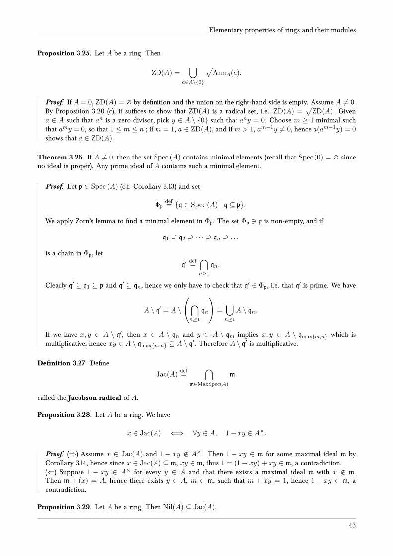
Elementary properties of rings and their modules
Proposition 3.25. Let A be a ring. Then
ZD(A) =⋃
a∈A\0
√AnnA(a).
Proof. If A = 0, ZD(A) = ∅ by definition and the union on the right-hand side is empty. Assume A 6= 0.By Proposition 3.20 (c), it suffices to show that ZD(A) is a radical set, i.e. ZD(A) =
√ZD(A). Given
a ∈ A such that an is a zero divisor, pick y ∈ A \ 0 such that any = 0. Choose m ≥ 1 minimal suchthat amy = 0, so that 1 ≤ m ≤ n ; ifm = 1, a ∈ ZD(A), and ifm > 1, am−1y 6= 0, hence a(am−1y) = 0shows that a ∈ ZD(A).
Theorem 3.26. If A 6= 0, then the set Spec (A) contains minimal elements (recall that Spec (0) = ∅ sinceno ideal is proper). Any prime ideal of A contains such a minimal element.
Proof. Let p ∈ Spec (A) (c.f. Corollary 3.13) and set
Φpdef= q ∈ Spec (A) | q ⊆ p.
We apply Zorn’s lemma to find a minimal element in Φp. The set Φp 3 p is non-empty, and if
q1 ⊇ q2 ⊇ · · · ⊇ qn ⊇ . . .
is a chain in Φp, let
q′def=⋂n≥1
qn.
Clearly q′ ⊆ q1 ⊆ p and q′ ⊆ qn, hence we only have to check that q′ ∈ Φp, i.e. that q′ is prime. We have
A \ q′ = A \
⋂n≥1
qn
=⋃n≥1
A \ qn.
If we have x, y ∈ A \ q′, then x ∈ A \ qn and y ∈ A \ qm implies x, y ∈ A \ qmaxm,n which ismultiplicative, hence xy ∈ A \ qmaxm,n ⊆ A \ q′. Therefore A \ q′ is multiplicative.
Definition 3.27. Define
Jac(A)def=
⋂m∈MaxSpec(A)
m,
called the Jacobson radical of A.
Proposition 3.28. Let A be a ring. We have
x ∈ Jac(A) ⇐⇒ ∀y ∈ A, 1− xy ∈ A×.
Proof. (⇒) Assume x ∈ Jac(A) and 1 − xy /∈ A×. Then 1 − xy ∈ m for some maximal ideal m byCorollary 3.14, hence since x ∈ Jac(A) ⊆ m, xy ∈ m, thus 1 = (1− xy) + xy ∈ m, a contradiction.(⇐) Suppose 1 − xy ∈ A× for every y ∈ A and that there exists a maximal ideal m with x /∈ m.Then m + (x) = A, hence there exists y ∈ A, m ∈ m, such that m + xy = 1, hence 1 − xy ∈ m, acontradiction.
Proposition 3.29. Let A be a ring. Then Nil(A) ⊆ Jac(A).
43

Chapter 3
Proof. This follows since
Nil(A) =⋂
p∈Spec(A)
p ⊆⋂
m∈MaxSpec(A)
m = Jac(A).
3.4 Prime Avoidance Lemma
Theorem 3.30. (Prime Avoidance Lemma) Let A be a ring and p1, . . . , pn be ideals such that p1, . . . , pn−2
are prime ideals. Let T ⊆ A a subset closed under addition and multiplication. Then
T ⊆n⋃i=1
pi =⇒ T ⊆ pi0 for some 1 ≤ i0 ≤ n.
Proof. For n = 1, this is clear. For n = 2, if T ⊆ a1∪a2 and T 6⊆ a1, a2, then we can find t1 ∈ T∩(a1\a2)and t2 ∈ T ∩ (a2 \ a1), so that t1 + t2 ∈ T ⊆ a1 ∪ a2. If t1 + t2 ∈ a1, then t2 ∈ a1, a contradiction ;similarly if t1 + t2 ∈ a2. It follows that T ⊆ a1 or T ⊆ a2.Suppose our statement holds for n − 1. We show the following claim : there exists j ∈ 1, . . . , n suchthat
T ∩ pj ⊆n⋃i=1i 6=j
pi.
Suppose such j does not exist. Then for each j, we have tj ∈ (T ∩ pj) \⋃ni=1i 6=j
pi. Consider
tdef= t1 +
n∏k=2
tk ∈ T
by the assumptions on T .For i = 1, t2, . . . , tn /∈ p1 hence
∏nk=2 tk /∈ p1 (use the fact that p1 is prime). Therefore, t1 ∈ p1 implies
t /∈ p1.For i > 1, since t1 /∈ pi but
∏nk=2 tk ∈ pi, t /∈ pi.
Therefore t /∈ pi for each i ∈ 1, . . . , n, hence t ∈ T \⋃ni=1 pi = ∅, a contradiction. This means that if
we let j be such that T ∩ pj ⊆⋃ni=1i 6=j
pi,
T ⊆n⋃i=1
pi =⇒ T =n⋃i=1
(T ∩ pi) ⊆n⋃i=1i 6=j
pi,
Our i0 exists by induction.
Remark 3.31. A second proof exists if we assume all the pi are prime (in the case where n = 2, it is thesame proof). We write it down for completeness.
We prove the contrapositive, i.e. if T 6⊆ pi for i = 1, · · · , n, then T 6⊆⋃ni=1 pi. We proceed by induction
on n. For n = 1, this is clear. Suppose the result is true for n − 1 but not for n. We deduce that for eachi = 1, · · · , n, there exists ti in the set
T ∩n⋂j=1
j 6=i
(A \ pj).
44

Elementary properties of rings and their modules
If for some i, we have ti /∈ pi, then ti /∈⋃ni=1 pi, so we are done. Otherwise, assume ti ∈ pi for i = 1, · · · , n
and consider the element
tdef=
n∑i=1
n∏j=1
j 6=i
tj ∈ T.
Computing modulo pi, we have t ≡n∏j=1
j 6=i
tj 6≡ 0 (mod pi), which shows that t /∈n⋃i=1
pi.
Theorem 3.32. (Prime Intersection Lemma) Let A be a ring, p a prime ideal and a1, · · · , an E A be idealssatisfying
⋂ni=1 ai ⊆ p. Then there exists 1 ≤ j ≤ n satisfying aj ⊆ p. If
⋂ni=1 ai = p, there exists
1 ≤ j ≤ n such that aj = p.
Proof. Suppose p 6⊆ ai for all 1 ≤ i ≤ n. Pick ai ∈ ai ∩ (A \ p) for 1 ≤ i ≤ n. Then∏ni=1 ai ∈
(A \ p) ∩⋂ni=1 ai ⊆ (A \ p) ∩ p = ∅, a contradiction. This proves the first part. For the second part, if
aj ⊆ p, then aj ⊆ p =⋂ni=1 ai ⊆ aj , so that p = aj .
45

Chapter 4
Properties of rings, part I
We introduce three classes of rings which only requires knowledge of rings at the level of elements : Euclideandomains, principal ideal domains (PIDs) and unique factorization domains (UFDs).
4.1 Euclidean domains
Definition 4.1. Let A be an integral domain. An Euclidean function on A is a function f : A \ 0 → Nwith the following property : for any a, b ∈ A with b 6= 0, there exists q, r ∈ A with either f(r) < f(b) orr = 0 such that a = qb+ r. The element q is called a quotient and r is called a remainder.
An Euclidean domain is an integral domain A for which an Euclidean function exists.
Remark 4.2. If A is an Euclidean domain and f : A \ 0 → N an Euclidean function, the function f iscertainly not unique with the above property. In fact, if g : N → N is any strictly increasing function, theng f is also an Euclidean function for A.
Theorem 4.3. (Euclidean Algorithm) Let A be an Euclidean domain and f an Euclidean function for A. Forany pair (a, b) with b 6= 0, there exists a finite sequence of succesive quotients and remainders (qi, ri)ni=0
starting with (q0, r0) the quotient and remainder of the pair (a, b) and terminating when rn+1 = 0, in whichcase we cannot compute a new quotient/remainder pair. This sequence is called the Euclidean algorithmand it satisfies the following equations :
a = q0b+ r0
b = q1r0 + r1
r0 = q2r1 + r2
...
rn−3 = qn−1rn−2 + rn−1
rn−2 = qnrn−1 + rn
rn−1 = qn+1rn.
Proof. We start by letting (q0, r0) be the quotient and remainder of the pair (a, b). If r0 = 0, westop the algorithm. Otherwise, the pair (b, r0) has a quotient/remainder pair (q1, r1) satisfying b =q1r0 + r1. Suppose we have computed the pair (qk, rk) and rk 6= 0. Then the pair (rk−1, rk) hasa quotient/remainder pair (qk+1, rk+1) ; if rk+1 = 0, the algorithms stops. If not, we continue thealgorithm by replacing the pair (rk−1, rk) by the pair (rk, rk+1).All there is left to show is that the algorithm must stop eventually. But this is clear since if it never
46

Elementary properties of rings and their modules
stopped, we would have found a sequence of integers
f(b) > f(r0) > f(r1) > · · · > f(rk) > · · · ≥ 0,
a contradiction.
Example 4.4. • Any field F is an Euclidean domain by letting f : F \ 0 → N be any function. Thisis because if a, b ∈ F with b 6= 0, we can always write a = (ab−1)b.
• The ring of integers Z is an Euclidean domain with the Euclidean function | · | : Z→ N given by theabsolute value :
|a| def=
a if a ≥ 0
−a if a < 0.
To see this, let a, b ∈ Z with b 6= 0. The real intervals [q|b|, (q + 1)|b|[ with q ∈ Z are disjoint andcover Z, so a must be in precisely one of them. Let q be the integer for which a ∈ [q|b|, (q + 1)|b|[and let r = a− q|b|. Then a = q|b|+ r and since 0 ≤ r < |b|, we have 0 ≤ |r| < |b|. If b > 0, we aredone ; if b < 0, we replace q by −q and preserve the equality a = qb+ r.
• If F is a field, then the polynomial ring F [x] is an Euclidean domain with Euclidean function sendingf(x) ∈ F [x] \ 0 to deg f , the degree of f :
deg f = deg
∗∑i≥0
aixi
def= mini ∈ N | ai 6= 0.
To see this, the fact that F [x] is an integral domain is clear (check the coefficients of highest degree) ;suppose f, g ∈ F [x] and g 6= 0. If deg f < deg g, we write f = 0 · g + f , which works by assumptionon f and g. If deg f ≥ deg g, write
f =
deg f∑i=0
aixi, g =
deg g∑i=0
bixi
so that
deg
(f −
adeg f
bdeg gxdeg f−deg gg
)< deg f
(note that f and adeg f
bdeg gxdeg f−deg gg both have degree deg f , but since they have the same coefficient
in front of xdeg f , the difference cancels it out). We let qdef=
adeg f
bdeg gxdeg f−deg g and r
def= f − qg, so that
deg r < deg f .
• Let d ∈ Z \0 and consider the polynomial x2 −D. The ringdef= Z[
√D] ⊆ C consists of Z-linear
combinations a + b√D with a, b ∈ Z. These expressions are added and multiplied just as integers,
with the rule that√D
2= D :
(a+ b√D) + (a′ + b′
√D) = (a+ a′) + (b+ b′)
√D
(a+ b√D)(a′ + b′
√D) = (aa′ + bb′D) + (ab′ + a′b)
√D.
For D = −1, we write idef=√D and the ring Z[i] is called the ring of Gaussian integers. One can
construct C as the quotient ring R[x]/(x2 + 1), turning the natural inclusion Z ⊆ R into the naturalinclusion Z[i] = Z[x]/(x2 + 1) ⊆ R[x]/(x2 + 1) = C ; the complex numbers a+ bi with a, b ∈ R thatare in Z[i] are precisely those for which a, b ∈ Z. Since Z[i] ⊆ C, Z[i] is an integral domain ; we willshow that Z[i] is also an Euclidean domain.
47

Chapter 4
Let N : Z[i] \ 0 → N be defined as N(a+ bi)def= a2 + b2 (in algebraic number theory, the function
N is called a norm). If α = a+ bi and β = c+ di 6= 0, in the field C, we have
α
β=a+ bi
c+ di
c− dic− di
=
(ac+ bd
c2 + d2
)︸ ︷︷ ︸
def= r
+
(bc− adc2 + d2
)︸ ︷︷ ︸
def= s
i.
Note that r, s ∈ Q \0. Let p, q ∈ Z be integers such that |r − p|2 + |s − q|2 < 1 (this can be doneby choosing p (resp. q) the closest integer to r (resp. s), in which case |r − p|2 + |s− q|2 ≤ 1/2). Set
θdef= (r − p) + (s− q)i = α
β − (p+ qi) and γdef= βθ. Then
γ = β
(α
β− (p+ qi)
)= α− β(p+ qi) ∈ Z[i], =⇒ α = (p+ qi)β + γ
As N is induced from the norm map on C, we have N(γ) = N(β)N(θ) < N(β), therefore showingthat N is an Euclidean function and Z[i] an Euclidean domain.
Definition 4.5. Let A be a ring. An ideal a E A is called principal if it can be generated by one element,i.e. if there exists a ∈ a with a = (a)A.
Theorem 4.6. Every ideal a E A is principal when A is an Euclidean domain. More precisely, if (0) 6= a EA, then a = (b)A where b has minimal norm in a.
Proof. If a = (0), there is nothing to prove. Assume a 6= (0) and pick b ∈ a of minimal norm. Theinclusion (b)A ⊆ a is obvious. For the reverse inclusion, pick a ∈ a and perform the Euclidean algorithm: we obtain a = qb + r with r = 0 or N(r) < N(b). Since a, b ∈ a, we have r = a − qb ∈ a, thereforeN(r) < N(b) is impossible by the minimality of N(b) ; this shows r = 0, so that a = qb ∈ (b)A.
Example 4.7. Of course, not every integral domain is an Euclidean domain. It suffices to consider F [x, y]and the ideal (x, y) ; if g(x, y) ∈ (x, y) and x = f(x)g(x) and y = f ′(x)g(x), since (x, y) containsno constant polynomials, we deduce that we have to assume deg g = 1 ; but x and y do not differ by apolynomial of degree 0, so we obtain a contradiction. In particular, F [x, y] is not a Euclidean domain.
Similarly, Z[x] is not a Euclidean domain because the ideal (2, x) is not principal. If g(x) were togenerate it, the equality 2 = f(x)g(x) implies that deg g = 0, i.e. g is an integer. Therefore g = ±2, whichimplies g does not generate (2, x).
4.2 Greatest common divisors and GCD domains
Definition 4.8. Let A be a ring and a, b ∈ A with b 6= 0.
(a) The element a is said to be a multiple of b if there exists c ∈ A with a = bc ; equivalently, if a ∈ (b)A.In this case, we call b a divisor of a and say that b divides a, which we denote by b | a.
(b) A greatest common divisor of a and b, both non-zero, is an element d ∈ A satisfying the following :
(i) d | a and d | b(ii) if d′ ∈ A satisfies d′ | a and d′ | b, then d′ | d.
A choice of greatest common divisor for a and b will be denoted by ddef= gcd(a, b). In integral
domains, the greatest common divisor is well-defined up to a unit, i.e. any two greatest commondivisors are associates ; however, it need not exist.
48

Elementary properties of rings and their modules
(c) Given a1, · · · , an ∈ A\0, a greatest common divisor of a1, · · · , an is an element d ∈ A satisfyingthe following :
(i) d | ai for 1 ≤ i ≤ n(ii) If d′ ∈ A satisfies d′ | ai for 1 ≤ i ≤ n, then d′ | d.
We denote the greatest common divisor of a1, · · · , an by ddef= gcd(a1, · · · , an).
(d) The ring A is a Bézout domain if it is an integral domain and for any a, b ∈ A, the ideal (a, b)A E Ais principal.
(e) The ring A is a GCD domain if it is an integral domain and for any a, b ∈ A, there exists a greatestcommon divisor of a and b.
Remark 4.9. In number theory, it is typical when computing greatest common divisors in Z that gcd(a, b)doesn’t denote any greatest common divisor generating (gcd(a, b)) but rather the positive generator of thatideal ; this is well-defined, but in more general rings there is no natural choice of the generator of the ideal(gcd(a, b)).
Proposition 4.10. The conditions of Definition 4.8 are equivalent to the following : if adef= (a, b) E A with
a, b ∈ A \ 0, then d is a greatest common divisor for a and b if and only if the two following conditionshold :
(i) a ⊆ (d)A
(ii) If d′ ∈ A is another element for which a ⊆ (d′)A, then (d)A ⊆ (d′)A.
Proof. It suffices to see that for an ideal a and a principal ideal (b) = b, a ⊆ b if and only if b dividesevery element of a. The latter is equivalent to b dividing a set of generators for a. The proof consists inusing this equivalence to translate the conditions from elements and divisibility to ideals and inclusions.
Remark 4.11. In other words, d is a greatest common divisor for a and b if and only if (d)A is a minimumin the set of principal ideals containing (a, b)A, partially ordered under inclusion. The same reasoning canbe done for n elements ; d is a greatest common divisor of a1, · · · , an ∈ A \ 0 if and only if (d)A is aminimum in the set of principal ideals containing (a1, · · · , an)A (see Proposition 4.12).
A priori, there is no reason to believe that such an ideal exists. Non-existence may happen if the set ofprincipal ideals containing (a, b)A admits more than one minimal element. However, if a greatest commondivisor exists, the ideal it generates is unique (by uniqueness of the minimum ; equivalently, if (d) and (d′)are generated by greatest common divisors, then (ii) says that (d) ⊆ (d′) and (d′) ⊆ (d), so (d) = (d′).Furthermore, if a greatest common divisor d of a and b exists, it is not necessary that (a, b) = (d). As astandard example, let A = F [x, y] where F is a field, a = x and b = y. If d divides x and y, then d ∈ F .In particular, A is the only principal ideal containing (x, y), so 1 = gcd(x, y) ; clearly (x, y)A 6= A.
As an example, let Z[√−3] ⊆ C be the Z-subalgebra generated by
√−3 =
√3i. Let
adef= 4 = 2 · 2 = (1 +
√−3)(1−
√−3), b = 2(1 +
√−3).
Clearly (a, b) ⊆ (2) and (a, b) ⊆ (1 +√−3). Letting N : Z[
√−3] → N denote the absolute value map in
C squared and restricted to Z[√−3], we have N(2) = 4 = N(1 +
√−3). Note that neither of the ideals (2)
and (1 +√−3) are contained in the other since the units of the integral domain Z[
√−3] are −1, 1 (use
the norm map!). In particular, 2 and 1 +√−3 are not greatest common divisors. A similar argument rules
out 1−√−3 and their multiples by a unit are of course also ruled out since these generate the same ideal.
Since these are the only divisors of 4 (use the norm map again!), a and b admit no greatest common divisor.
49

Chapter 4
Proposition 4.12. Let A be a GCD domain. If a1, · · · , an ∈ A \ 0, then a greatest common divisor ofa1, · · · , an exists and can be constructed recursively via the formula
gcd(a1, · · · , an) = gcd(gcd(a1, · · · , an−1), an)
Proof. Let ddef= gcd(gcd(a1, · · · , an−1), an). Then d divides an and gcd(a1, · · · , an−1), so d also
divides a1, · · · , an−1. If d′ divides a1, · · · , an, then it also divides a1, · · · , an−1, hence dividesgcd(a1, · · · , an−1). Since it also divides an, it divides their greatest common divisor, which is d.
Lemma 4.13. Let A be an integral domain. If d, d′ ∈ A satisfy (d)A = (d′)A, then there is a uniqueunit u ∈ A× such that d′ = ud (and d = u−1d′). In particular, greatest common divisors (of two non-zeroelements or a finite set of non-zero elements) are uniquely determined up to multiplication by a unit elementwhen they exist.
Proof. The equality (d)A = (d′)A implies that d′ = ud and d = u′d′, so that d = uu′d and uu′ = 1. Thisimplies that
Theorem 4.14. Let A be an Euclidean domain and a, b ∈ A \ 0. Let ddef= rn be the last non-zero
remainder in the Euclidean algorithm. Then
(i) d is a greatest common divisor for a and b
(ii) We have (d)A = (a, b)A. In particular, d can be written as an A-linear combination of a and b, thatis, there are elements x, y ∈ A such that
d = ax+ by.
Proof. Recall the construction : the sequence (qi, ri)ni=0 is chosen so that
a = q0b+ r0
b = q1r0 + r1
r0 = q2r1 + r2
...
rn−3 = qn−1rn−2 + rn−1
rn−2 = qnrn−1 + rn
rn−1 = qn+1rn = qn+1d.
One sees that d = rn | rn and d | rn−1 by the last equation. The equations ri = qi+2ri+1 + ri+2 impliesthat if d divides ri+1 and ri+2, then d divides ri. Going up the set of equations by induction, we see thatd | b and d | a. This shows that (a, b)A ⊆ (d)A.Re-writing the set of equations above as
a− q0b = r0
b− q1r0 = r1
r0 − q2r1 = r2
...
rn−3 − qn−1rn−2 = rn−1
rn−2 − qnrn−1 = rn
rn−1 − qn+1rn = qn+1d,
50

Elementary properties of rings and their modules
we see that by the first equation, r0 ∈ (a, b), and by the second equation, r1 ∈ (a, b). The rest of theequations show by recursion that if ri, ri+1 ∈ (a, b), then ri+2 ∈ (a, b). This shows that d = rn ∈ (a, b),i.e. (d)A ⊆ (a, b)A, therefore giving (d)A = (a, b)A. In particular, d ∈ (a, b)A, which gives the existenceof the linear combination.
4.3 Principal ideal domains
Definition 4.15. A principal ideal domain (written PID for short) is an integral domain in which everynon-zero ideal is principal. (By Theorem 4.6, Euclidean domains are PIDs.)
Example 4.16. Fields are trivially principal ideal domains since the only non-zero ideal is the field itself.We have seen that Euclidean domains are also principal ideals domains (c.f. Theorem 4.6). There are,however, principal ideal domains which are not Euclidean domains. The examples are a bit too involved todescribe them at the moment : one is the ring of integers of Q(
√D) where D = −19,−43,−67 or −163 ;
another is the localization of the power series ring K[[x, y]] at the polynomial x2 + y3.
Proposition 4.17. Let A be a PID. Every non-zero prime ideal p ∈ Spec (A) is maximal, i.e. Spec (A) =MaxSpec (A) ∪ (0).
Proof. Let (p)A = p ∈ Spec (A) \ (0). By Krull’s theorem, let (m)A = m ∈ MaxSpec (A) with p ⊆ m.Since p ∈ (m)A, p = am ∈ p for some a ∈ A. But p is a prime ideal, hence a ∈ p or m ∈ p. If a ∈ p, wecan write a = bp so that p = am = bmp and bm = 1, which means m contains a unit ; a contradiction.Therefore m ∈ p, m ⊆ p ⊆ m and thus m = p is maximal.
Corollary 4.18. If A is a ring and A[x] is a PID, then A is a field.
Proof. Since A[x] must be an integral domain and A is a subring, A is also an integral domain. ThereforeA[x]/(x)A ' A is an integral domain, meaning (x)A is a non-zero prime ideal, thus maximal. We deducethat A ' A[x]/(x)A is a field.
Definition 4.19. Let A be an integral domain and let a, p ∈ A \ (A× ∪ 0).
(i) The element a is called irreducible in A if whenever a = bc with b, c ∈ A then either b ∈ A× orc ∈ A×. Otherwise we say a is reducible, in which case there exists a factorization a = bc where band c are not units.
(ii) The element p ∈ A is called a prime in A if pdef= (p)A ∈ Spec (A). In other words, p is prime if
whenever p | ab, then p | a or p | b.
(iii) Two arbitrary elements a, b ∈ A are said to be associates if there exists a unit u ∈ A× such thata = ub.
Proposition 4.20. Let A be an integral domain.
(i) The relation a ∼ b if a and b are associates is an equivalence relation, thus partitions A. Notableequivalence classes are A× and 0.
(ii) A prime element p ∈ A is irreducible.
(iii) If A is a PID, then p ∈ A is prime if and only if it is irreducible.
51

Chapter 4
Proof. For (i), the relation a ∼ b is obvious reflexive and symmetric. For transitivity, if a = ub and b = u′cwhere u, u′ ∈ A×, then a = uu′c. Note that c = u · 0 implies c = 0 and any unit u is equivalent to 1since 1 = u−1u.For (ii), suppose p = (p) is a non-zero prime ideal and p = ab. Then p | ab, thus without loss of generalityassume p | a. Write a = pr, so that p = ab = prb. This means b is a unit, i.e. p is irreducible.An equivalent way to phrase the definition of an irreducible element is that a is irreducible if (a)A E Ais maximal among the subset PIdeal (A) ⊆ Ideal (A) of principal ideals not equal to (1)A = A. Forif (a)A ⊆ (b)A, then a = bc. If b is a unit, (b)A = A, a contradiction ; therefore c is a unit, so that(a)A = (b)A. If A is a PID, an irreducible element a generates a maximal ideal m = (a)A, which isprime.
4.4 Unique factorization domains
Definition 4.21. A unique factorization domain (or UFD for short) is an integral domain A with the twofollowing properties :
(i) (Existence of the factorization) Any a ∈ A \ (A× ∪0) can be written as a product of not necessarilydistinct irreducible elements pi, i.e. a = p1 · · · pn
(ii) (Unicity of the factorization) If two factorizations into irreducible are equal, namely p1 · · · pn =q1 · · · qm, then n = m and there is a bijection σ : 1, · · · , n → 1, · · · , n such that pi andqσ(i) are associates.
Theorem 4.22. Let A be a UFD. Then a ∈ A \ (A× ∪ 0) is prime if and only if it is irreducible.
Proof. By Proposition 4.20, it suffices to prove that irreducible elements are prime. Let p be an irreducibleelement and assume p | ab. There exists c ∈ A with cp = ab. Writing a = p1 · · · pn and b = q1 · · · qm,writing c as a product of irreducibles, by Definition 4.21 (ii), the irreducible element p is associate to eitherone of the pi’s or one of the qi’s. Without loss of generality, assume p and p1 are associates so that wehave u ∈ A× with up = p1. Therefore (up2 · · · pn)p = p1 · · · pn = a, meaning p | a. This means p isprime.
Lemma 4.23. Let A be a UFD and a, b ∈ A\0. Write a = upe11 · · · penn , b = vpf11 · · · p
fnn where p1, · · · , pn
are distinct primes in the factorization of a into irreducibles, ei, fi ≥ 0 and u, v are units. Then a divides bif and only if ei ≤ fi for i = 1, · · · , n.
Proof. If a divides b, then there exists c = wpg11 · · · p
gnn q1 · · · qm such that ca = b and the qi’s are primes
distinct from the pi. It follows that ei ≤ ei + gi = fi. Conversely, letting c = vu−1pf1−e11 · · · pfn−enn , we
have ac = b, so a | b.
Corollary 4.24. Let A be a UFD, a, b ∈ A \ 0 and suppose a = upe11 · · · penn , b = vpf11 · · · p
fnn are
factorizations of a and b into distinct primes p1, · · · , pn with multiplicities ei, fi ≥ 0 where u, v ∈ A×.Then the element
d = pmine1,f11 · · · pminen,fn
n
is a greatest common divisor for a and b.
More generally, if a1, · · · , am ∈ A \ 0, writing ai = uipei,11 · · · pei,nn for 1 ≤ i ≤ m, the element
d = pmine1,1,··· ,em,11 · · · pmine1,n,··· ,em,n
n
is a greatest common divisor for a1, · · · , am.
52

Elementary properties of rings and their modules
Proof. By Lemma 4.23, d divides both a and b. If d′ divides both a and b, then d = wpg11 · · · p
gnn where
w is a unit and gi ≥ 0 ; Lemma 4.23 again shows that gi ≤ ei, fi, hence gi ≤ minei, fi. ApplyingLemma 4.23 a third time, we see that d′ divides d. Therefore d is a greatest common divisor for a and b.The formula for the greatest common divisor follows from Proposition 4.12.
Lemma 4.25. Let A be an integral domain.
(i) If A is a PID, then A is a Bézout domain.
(ii) If A is a Bézout domain, then A is a GCD domain and any finitely generated ideal is principal.
(iii) If A is a UFD, then A is a GCD domain.
Proof. (i) Any ideal of A is principal, hence also those generated by two elements.
(ii) Since (a, b) is principal, the ideal (a, b) is minimal among the principal ideals containing it, thusany generator d for the ideal is a greatest common divisor. It follows that A is a GCD domain.
Let a = (a1, · · · , an). We treat the case n ≥ 2 by induction on n. For n = 2, this is the hypothesis.For n > 2,
(a1, · · · , an−2, an−1, an) = (a1, · · · , an−2 ∪ (an−1, an))
= (a1, · · · , an−2 ∪ (d))
= (a1, · · · , an−2, d).
Since the latter has n− 1 generators, it is principal.
(iii) This follows from Corollary 4.24.
Theorem 4.26. A principal ideal domain A is a unique factorization domain.
Proof. Let a ∈ A\(A×∪0). If a is irreducible, we have already found its factorization into irreducibles,namely itself. If not, then a is reducible ; write a = a1a2. If both a1, a2 are irreducible, we are done.Otherwise, we factor a1 = a11a12 and a2 = a21a22 with one of the aij ’s possibly a unit.Suppose we repeated this process k times. Then we have a factorization a =
∏2i1,··· ,ik=1 ai1···ik . If all
the ai1···ik are irreducibles or units, we are done. Otherwise, each ai1···ik which is a unit or irreducible
is factored as ai1···ik = ai1···ik1ai1···ik2 with ai1···ik1def= ai1···ik and ai1···ik2
def= 1, and each ai1···ik which is
reducible admits a factorization ai1···ik = ai1···ik1ai1···ik2.We repeat this construction inductively. If it eventually stops at the kth step, this means that all the ai1···ikare irreducibles or units, so we have found a factorization for a. If it doesn’t stop, there is an infinitesequence (i1, · · · , in, · · · ) of 1’s and 2’s with
(a) ( (ai1) ( (ai1i2) ( · · · ( (ai1···in) ( · · · .
By Proposition 2.2, the union of the ideals in that chain are an ideal of A which is then principal, i.e.generated by some b ∈ A. Since b lies in the union of all the ideals in the chain, it must lie in some idealin the chain ; this shows that (b)A equals the union of only finitely members of the chain, a contradictionto the strict inclusions obtained at each step. This proves existence of the factorization.For unicity, suppose p1 · · · pn = q1 · · · qm are two factorizations of the same element a ∈ A \ (A× ∪ 0).Note that n,m ≥ 1 by Krull’s theorem since (0) 6= (a) 6= A. Without loss of generality, assumen ≤ m. Since pn is irreducible, it is prime by Theorem 4.22. Therefore pn divides q1 · · · qm, hence upto a permutation of the factors we can assume pn divides qm. Since qm is irreducible, pn and qm areassociates. Writing qm = upn, we can replace qm−1 by uqm−1 and cancel out pn (because we are in an
53

Chapter 4
integral domain) so that p1 · · · pn−1 = q1 · · · qm−1. By descending induction on n, we reduce to the casen = 1 which means p1 = q1 · · · qm. Since all the elements involved are irreducible, we must have m = 1,so in particular p1 and q1 are associates.
Remark 4.27. We have implicitly proved that a PID is a noetherian ring, a property which we will discussin further detail in Chapter 9.
Corollary 4.28. The ring Z is a unique factorization domain.
Proof. We have proved in Example 4.4 that the Euclidean algorithm holds for Z with the absolute valueas a Euclidean function. Therefore Z is a Euclidean domain, hence a PID by Theorem 4.6, thus a uniquefactorization domain by Theorem 4.26.
4.5 Extensions and contractions
Definition 4.29. Let f : A→ B be a morphism of rings, a E A and b E B.
(a) The contraction of b E B is the ideal f−1(b). If the morphism f is understood, we denote thecontraction of b by f with bc.
(b) The extension of a E A is the ideal generated by a in B, namely (a)B . If the morphism f isunderstood, we denote the extension of a by f with ae.
Remark 4.30. Any morphism of rings f : A → B can be factored as Ap−→ f(A)
g−→ B. For p,understanding extensions and contractions is very simple since the image of an ideal (resp. prime ideal) viaa surjective map is an ideal (resp. prime ideal) ; we even have a bijective correspondence between ideals inf(A) and ideals in A lying above ker f (c.f. Theorem 1.26 and Remark 3.23). However, the situation for gis not always as clear.
For instance, consider the inclusion map g : Z → Z[i] where i ∈ C satisfies i2 = −1. Given a primenumber p ∈ Z, one can show the following :
(i) For p = 2, the prime ideal (2)Z[i] satisfies (2)eZ = (2)Z[i] = (1 + i)Z[i](1− i)Z[i] = (1 + i)2
Z[i]
(ii) If p ≡ 1 (mod 4), one can find two positive integers a, b > 0 such that p = a2 + b2 = (a− bi)(a+ bi),so that (p)Z[i] = (a+ bi)Z[i](a− bi)Z[i] ; furthermore, those factors are prime ideals
(iii) If p ≡ 3 (mod 4), the ideal (p)Z[i] is prime.
We will be more interested in these number-theoretic questions when we study Dedekind domains in Chap-ter 19.
Proposition 4.31. Let f : A → B be a morphism of rings and a E A, b E B. Then a ⊆ bc if and onlyif ae ⊆ b, so the maps (−)e : Ideal (A) → Ideal (B) and (−)c : Ideal (B) → Ideal (A) form a Galoisconnection. In particular,
(i) For any a E A and b E B, the following holds :
a ⊆ aec, b ⊇ bce, ae = aece, bc = bcec.
(ii) We have an inclusion-preserving bijective correspondence :
b E B | bce = b b7→bc
←−−−−−→ae← [a
a E A | aec = a.
54

Elementary properties of rings and their modules
Proof. The first statement is equivalent to a ⊆ f−1(b) if and only if (f(a))B ⊆ b, which is trivial sincethe latter is equivalent to f(a) ⊆ b. The other statements follow from the general theory of Galoisconnections.
Proposition 4.32. Let f : A→ B be a morphism of rings, a, a1, a2 E A and b, b1, b2 E B be ideals. Thenthe following holds :
(a1 + a2)e = ae1 + ae
2, (b1 + b2)c ⊇ bc1 + bc
2
(a1 ∩ a2)e ⊆ ae1 ∩ ae
2, (b1 ∩ b2)c = bc1 ∩ bc
2
(a1a2)e = ae1a
e2, (b1b2)c ⊇ bc
1bc2
(a1 : a2)e ⊆ (ae1 : ae
2), (b1 : b2)c ⊆ (bc1 : bc
2)√a
e ⊆√ae,
√b
c ⊆√bc.
Proof. The first three properties in each column are trivial and their proof are omitted ; it suffices towrite them down explicitly. The inclusion (a1 : a2)e ⊆ (ae
1 : ae2) is equivalent to
f((a1 : a2)) ⊆ ((f(a1))B : (f(a2))B)
which is clear since if x ∈ A is such that for all y ∈ a1, we have xy ∈ a2, then f(x) is such that for allf(y) ∈ f(a1), f(x)f(y) = f(xy) ∈ f(a2). The inclusion (b1 : b2)c ⊆ (bc
1 : bc2) is equivalent to
f−1(b1 : b2) ⊆ (f−1(b1) : f−1(b2))
so let x ∈ A be such that f(x) ∈ (b1 : b2), i.e. for all y ∈ b1, f(x)y ∈ b2. If z ∈ f−1(b1), thenxz ∈ f−1(b2) since f(xz) = f(x)f(z) ∈ b2. This proves the inclusion holds.The fifth inclusion in the first column is equivalent to f(
√a) ⊆
√(f(a))B and is obvious : if x ∈ A
satisfies xn ∈ a, then f(x)n ∈ f(a) ⊆ (f(a))B , hence f(x) ∈√
(f(a))B . The last inclusion is equivalentto f−1(
√b) ⊆
√f−1(b), so let x ∈ f−1(
√b). Then f(x)n ∈ b for some n ≥ 1, hence xn ∈ f−1(b), e.g.
x ∈√f−1(b).
4.6 Polynomial rings
Definition 4.33. Let A be a ring and E ⊆ A a subset. We denote by E[x] ⊆ A[x] the subset of polynomialswith coefficients in E, namely
a[x]def=
∗∑i≥0
aixi
∣∣∣∣∣∣ ∀i ≥ 0, ai ∈ E
.
We note that if a E A is an ideal, then a[x] E A[x]. For n > 1, we recursively define E[x1, · · · , xn]def=
(E[x1, · · · , xn−1])[xn].
Proposition 4.34. (Study of the polynomial ring in one variable) Let A be a ring and f =∑n
i=0 aixi ∈ A[x].
(a) The polynomial f is nilpotent if and only if a0, · · · , an ∈ Nil(A). In other words, Nil(A[x]) =Nil(A)[x]. In particular, A[x] is reduced if and only if A is reduced.
(b) The polynomial f is a unit if and only if a0 ∈ A× and a1, · · · , an ∈ Nil(A). In particular, if A isreduced, A[x]× = A×.
(c) The following are equivalent :
(i) A is a field
55

Chapter 4
(ii) A[x] is an Euclidean domain
(iii) A[x] is a PID
When any of the equivalent statements above hold, the Euclidean norm can always be taken to be thedegree of a polynomial.
(d) The polynomial f is a zero divisor if and only if there exists a ∈ A \ 0 such that af = 0.
(e) We have ZD(A[x]) ⊆ (ZD(A))[x]. Furthermore, A[x] is an integral domain if and only if A is anintegral domain.
(f) Let C : A[x] → Ideal (A) be the function defined for f =∑n
i=0 aixi by C(f) = (a0, · · · , an),
called the content of f . We say that f ∈ A[x] is primitive if C(f) = A. If f, g ∈ A[x], thenC(fg) ⊆ C(f)C(g). Furthermore, fg is primitive if and only if f and g are primitive.
(g) We have Jac(A[x]) = Nil(A[x]) = Nil(A)[x].
(h) If a E A is prime (resp. radical), then a[x] E A[x] is prime (resp. radical).
Proof. (a) Since Nil(A[x]) E A[x], if a0, · · · , an ∈ Nil(A), we see that aixi ∈ Nil(A[x]), hence sodoes f . Conversely, we proceed by induction on deg f . If fm = 0, then (anx
n)m = amn xnm is the
leading term of fm, thus amn = 0. It follows that f − anxn ∈ A[x] is also nilpotent and has smallerdegree, so by induction, a0, a1, · · · , an ∈ Nil(A). The equation Nil(A[x]) = (Nil(A))A[x] clearlyimplies Nil(A) = 0 if and only if Nil(A[x]) = 0, which gives the last statement.
(b) (⇐) By Proposition 1.38, if ai is nilpotent, so is aixi and∑n
i=1 aixi (because Nil(A[x]) E A[x]),
hence a0 +∑n
i=1 aixi = a0 is a unit (because A× ⊆ A[x]× is obvious). Conversely, clearly fg = 1
implies f(0)g(0) = 1, so f(0) = a0 is a unit (with inverse g(0)). We prove by induction on1 ≤ r ≤ m that ar+1
n bm−r = 0 ; since b0 ∈ A×, this will show that am+1n = 0. Equivalently, we
prove that ainbj = 0 when i ≥ m− j + 1.
Since fg = 1, we have
1 =
(n∑i=0
aixi
) m∑j=0
bjxj
=n+m∑k=0
(k∑i=0
aibk−i
)xk
which means that for all k ≥ 1,∑k
i=0 aibk−i = 0 (for this expression to make sense, we set
a` = bs = 0 when ` > n and s > m). Set rdef= m + n − k. Shifting indices and removing zero
terms, this gives
0 =m+n−r∑i=0
aibm+n−r−i =
n∑i=0
aibm+n−r−i =n∑i=0
an−ibm−r+i =r∑i=0
an−ibm−r+i.
For example, for r = 0, we get anbm = 0. For r = 1, an−1bm + anbm−1 = 0. Multiplying by an,we get
0 = an−1anbm︸ ︷︷ ︸=0
+ a2nbm = a2
nbm.
More generally, by induction on r ≥ 0, we have
0 = arn
(r∑i=0
an−ibm−r+i
)= ar+1
n bm−r +
r∑i=1
an−iarnbm−r+i︸ ︷︷ ︸
=0
= ar+1n bm−r.
The terms underbracketed vanish since m− (m− r + i) + 1 = r − (i− 1) ≤ r.
56

Elementary properties of rings and their modules
(c) ( (i) =⇒ (ii) ) Let f, g ∈ A[x] and assume deg fdef= n ≥ m
def= deg g. Write f =
∑ni=0 aix
i andg =
∑mj=0 bjx
j . Since A is a field, bm ∈ A×, hence
deg
(f − anx
n−m
bmg
)< deg f.
Let f1def= f − anxn−m
bm. If deg(f1) ≥ deg g, repeat the argument by replacing f by f1 and
construct f2, etc. This descent argument can be repeated finitely many times and stops whendeg(fk) < deg g, in which case
f = f1 +anx
n−m
bmg =
(f2 +
adeg f1xdeg f1−m
bmg
)+anx
n−m
bm= · · · = fk + hg, h ∈ A[x].
It follows that A[x] is an Euclidean domain.
( (ii) =⇒ (iii) ) This follows from Theorem 4.6.
( (iii) =⇒ (i) ) This is Corollary 4.18.
In particular, since (ii) implies (iii) implies (i) for whatever choice of Euclidean norm on A[x], wededuce that the degree becomes an Euclidean norm on A[x] as soon as A[x] is an Euclideandomain.
(d) Let g =∑m
j=0 bjxj ∈ A[x] with bm 6= 0 be of minimal degree such that fg = 0. Using the same
argument as in the proof of (b), this implies anbm = 0. The expression f(ang) = an(fg) = 0together with deg(ang) < deg g implies ang = 0. We show by induction on 0 ≤ r ≤ n (starting atr = n) that an−rg = 0. The equation fg = 1 in (b) implied
r∑i=0
an−ibm−r+i = 0
for r = 0, · · · ,m + n − 1 ; in this case, fg = 0 implies the equation also holds for r = m + n(although we only need these equations up to n). Note that the equation an−rg = 0 impliesan−rbi = 0 for all i ≥ 0. Suppose ang = · · · = an−(r−1)g = 0. Then
an−rbm =
r∑i=0
an−ibm−r+i = 0,
and as with the case of an, since deg(an−rg) < deg g, the expression f(an−rg) = an−r(fg) = 0implies an−rg = 0. We can deduce from this that aibj = 0 for i, j ≥ 0, e.g. b0f = · · · = bmf = 0.
Letting adef= bm 6= 0 proves the result.
(e) Note that if A = 0, A[x] = 0, hence we have nothing to prove, so assume A 6= 0. By (c), if f isa zero divisor, letting a ∈ A \ 0 be such that af = 0, a coefficient of f always becomes zerowhen multiplied by a, hence is a zero divisor ; this gives ZD(A[x]) ⊆ (ZD(A))[x]. The inclusionA ⊆ A[x] shows that if A[x] is an integral domain, so is A. Conversely, if ZD(A) = 0, then0 = (ZD(A))[x] ⊇ ZD(A[x]), thus A[x] is an integral domain.
(f) Write f =∑n
i=0 aixi, g =
∑mj=0 bjx
j . We notice that
C(f) = (a0, · · · , an), C(g) = (b0, · · · , bm),
C(fg) =
(k∑i=0
aibk−i
∣∣∣∣∣ 0 ≤ k ≤ m+ n
).
It follows that C(f)C(g) = (aibj | i, j ≥ 0) ⊇ C(fg).
57

Chapter 4
(⇒) Suppose fg is primitive, i.e. C(fg) = A. If C(f),C(g) 6= A, then by Corollary 2.10,
A = C(fg) ⊆ C(f)C(g) ( A,
a contradiction. Therefore either C(f) = A or C(g) = A. If C(f) = A, then A = C(fg) ⊆ C(g)implies C(g) = A ; the other case is symmetric.
(⇐) Suppose there exists f, g ∈ A[x] primitive with fg not primitive. By Krull’s theorem (c.f.
Corollary 3.12), let m ⊇ C(fg) be a maximal ideal and consider the ring Bdef= A/m 6= 0. The
polynomials f , g ∈ B[x] defined by the same coefficients but read modulo m are still primitive (andin particular non-zero) since 1 ∈ C(f),C(g) implies 1 + m ∈ C(f),C(g). It follows that f , g areprimitive and C(f g) = 0, i.e. f g = 0. Without loss of generality, assume f, g are primitive withfg = 0 and that A is a field (after replacing A by B), so that A[x] is an integral domain by (d).The equation f g = 0 implies f = 0 or g = 0, a contradiction to both being primitive.
(g) We already have Nil(A)[x] = Nil(A[x]) ⊆ Jac(A[x]) by (a) and Proposition 3.29. To show thatJac(A[x]) ⊆ Nil(A)[x], suppose f ∈ Jac(A[x]). By Proposition 3.28, 1 − xf ∈ A[x]× and by (b),we see that all the coefficients of 1 − xf of non-zero degree are nilpotent ; these are precisely thenegatives of the coefficients of f , hence f ∈ Nil(A)[x].
(h) If a is prime, then A/a is an integral domain, thus (A/a)[x] ' A[x]/a[x] is an integral domain,i.e. a[x] is prime. Similarly, if a is radical, then Nil((A/a)[x]) = Nil(A/a)[x] = 0 correspondsto Nil(A[x]/a[x]) under the isomorphism (A/a)[x] ' A[x]/a[x], hence a[x] =
√a[x] is a radical
ideal.
Definition 4.35. Let A be a ring. For f ∈ A[x1, · · · , xn], we use the notation
f =
∗∑i1,··· ,in≥0
ai1···inxi11 · · ·x
inn .
For f 6= 0, let
deg fdef= maxi1 + · · ·+ in | ai1···in 6= 0
denote the total degree of f . If d = deg f , we can re-arrange the above sum as
f =d∑i=0
∑i1+···+in=ii1,··· ,in≥0
ai1···inxi11 · · ·x
inn .
For i = 1, · · · , n, write degxi f for the degree of f when we see it as a polynomial in the variablexi with coefficients in A[x1, · · · , xi, · · · , xn] (since we have an obvious isomorphism A[x1, · · · , xn] 'A[x1, · · · , xi, · · · , xn][xi], where xi denotes omission of xi).
Proposition 4.36. (Study of the polynomial ring in several variables) Let A be a ring.
(a) The polynomial f is nilpotent if and only if ai1···in ∈ Nil(A) for all i1, · · · , in ≥ 0. In other words,Nil(A[x1, · · · , xn]) = (Nil(A))[x1, · · · , xn]. In particular, A[x1, · · · , xn] is reduced if and only if Ais reduced.
(b) The polynomial f ∈ A[x1, · · · , xn] is a unit if and only if a0···0 ∈ A× and ai1···in ∈ Nil(A) wheneveri1 + · · ·+ in > 0. In particular, if A is reduced, A[x1, · · · , xn]× = A×.
(c) The polynomial f is a zero divisor if and only if there exists a ∈ A \ 0 such that af = 0.
58

Elementary properties of rings and their modules
(d) We have ZD(A[x1, · · · , xn]) ⊆ (ZD(A))[x1, · · · , xn]. Furthermore, A[x1, · · · , xn] is an integral do-main if and only if A is an integral domain.
(e) Let C : A[x1, · · · , xn] → Ideal (A) be the function defined by C(f)def= (ai1···in | i1, · · · , in ≥ 0),
called the content of f . We say that f ∈ A[x1, · · · , xn] is primitive if C(f) = A. If f, g ∈A[x1, · · · , xn], then C(fg) ⊆ C(f)C(g). Furthermore, fg is primitive if and only if f and g areprimitive.
(f) We have Nil(A)[x1, · · · , xn] = Nil(A[x1, · · · , xn]) = Jac(A[x1, · · · , xn]).
(g) If a E A is prime (resp. radical), then a[x1, · · · , xn] E A[x1, · · · , xn] is prime (resp. radical).
Proof. (∗) Let d1, · · · , dn ≥ 1 be integers and for i = 1, · · · , n, let eidef=∏i−1j=1 dj (in particular, e1 = 1).
Consider the mapΦd1,··· ,dn : A[x1, · · · , xn]→ A[x], xi 7→ xei .
given by the universal property of the free A-algebra (c.f. Theorem 1.56). This map has the property thatif f, g ∈ A[x1, · · · , xn] satisfy degxi(f), degxi(g) < di for i = 1, · · · , n, then Φd1,··· ,dn(f) = Φd1,··· ,dn(g)implies f = g. This is because
Φd1,··· ,dn
∗∑i1,··· ,in≥0
ai1···inxi11 · · ·x
inn
=∑
i1,··· ,in≥0
ai1···inxe1i1+···+enin
and one checks using elementary number theory that there are no two distinct n-tuples (i1, · · · , in) and(i′1, · · · , i′n) with ij < dj for j = 1, · · · , n and
∑nj=1 ejij =
∑nj=1 eji
′j (compute modulo e2 to see that
i1 = i′1, subtract them from the equation and divide by d1 ; repeat inductively). We deduce that we cancompare the coefficients of Φd1,··· ,dn(f) and Φd1,··· ,dn(g) to decide if f = g.
(a) By induction on n, for which the case n = 1 is given by Proposition 4.34. Letting B =A[x1, · · · , xn−1], we have
Nil(A[x1, · · · , xn]) = Nil(B[xn])
= (Nil(B))[xn]
= (Nil(A[x1, · · · , xn−1]))[xn]
= ((Nil(A))[x1, · · · , xn−1])[xn]
= (Nil(A))[x1, · · · , xn].
(b) By induction on n, from which the case n = 1 is given by Proposition 4.34 (b). Let Bdef=
A[x1, · · · , xn−1] so that f ∈ A[x1, · · · , xn] can be seen as an element of B[xn] ; let F ∈ B[xn]be the polynomial in one variable corresponding to f and write F =
∑i≥0 gix
in where gi ∈ B for
i ≥ 0. We deduce that f ∈ A[x1, · · · , xn]× if and only if g0 ∈ B× and gi ∈ Nil(B) for i > 0. SinceNil(B) = Nil(A[x1, · · · , xn−1]) = (Nil(A))[x1, · · · , xn−1], this is equivalent to all the coefficientsinvolving the gi for i > 0 being nilpotent. For those involving g0 ∈ B× = A[x1, · · · , xn−1]×, theinduction hypothesis completes the proof.
(c) Let us use (∗). Write f =∑∗
i1,··· ,in≥0 ai1···inxi11 · · ·xinn . If f is a zero divisor, let the polynomial
g ∈ A[x1, · · · , xn] \ 0 be such that fg = 0 and write g =∑∗
j1,··· ,jn≥0 bj1···jnxi11 · · ·x
jnn . Pick
d1, · · · , dn such that di ≥ maxdegxi f,degxi g for i = 1, · · · , n. It follows that
0 = Φd1,··· ,dn(fg) = Φd1,··· ,dn(f)Φd1,··· ,dn(g)
hence both are zero divisors in A[x] ; we deduce that there exists a ∈ A \ 0 such that
0 = aΦd1,··· ,dn(f) = Φd1,··· ,dn(a)Φd1,··· ,dn(f) = Φd1,··· ,dn(af),
59

Chapter 4
from which we deduce af = 0 since degxi f ≥ degxi(af). The converse is trivial.
(d) By induction on n, from which the case n = 1 is given by Proposition 4.34 (d). We then have
ZD(A[x1, · · · , xn]) = ZD(A[x1, · · · , xn−1][xn])
⊆ (ZD(A[x1, · · · , xn−1]))[xn]
⊆ ((ZD(A))[x1, · · · , xn−1])[xn]
= (ZD(A))[x1, · · · , xn].
By induction on n again, A[x1, · · · , xn] is an integral domain if and only if A[x1, · · · , xn−1] is,which is then equivalent to A being an integral domain.
(e) We use (∗) again in the same way as in (c). Let f, g ∈ A[x1, · · · , xn] \ 0 and choose d1, · · · , dnthe same way as in (c). Since f and Φd1,··· ,dn(f) have the same set of non-zero coefficients, we haveC(f) = C(Φd1,··· ,dn(f)), hence the result follows by Proposition 4.34.
(f) Two proofs are possible. The first one is to use the same proof as in Proposition 4.34 (f) by replacing
the use of x ∈ A[x] by x1 ∈ A[x1, · · · , xn]. The second is to let Bdef= A[x1, · · · , xn−1] and
Nil(A[x1, · · · , xn]) = Nil(B[xn]) = Jac(B[xn]) = Jac(A[x1, · · · , xn]).
(g) This follows by induction on n using Proposition 4.34.
Definition 4.37. Let A be a ring. Recall Example 1.4 where we defined the power series ring with coefficientsin A, which we denoted by A[[x]]. Given a subset E ⊆ A, we denote by E[[x]] ⊆ A[[x]] the subset
E[[x]]def=
f ∈ A[[x]]
∣∣∣∣∣∣ f =∑i≥0
aixi, ai ∈ E
.
If B ⊆ A is a subring, then B[[x]] ⊆ A[[x]] is also a subring ; furthermore, if a E A, then a[[x]] E A[[x]].
We also define A[[x1, · · · , xn]]def= (A[[x1, · · · , xn−1]])[[xn]] for n > 1, the power series ring in n
variables. Furthermore, we set E[[x1, · · · , xn]]def= (E[[x1, · · · , xn−1]])[[xn]]. We write the elements of
A[[x1, · · · , xn]] asf =
∑i1,··· ,in≥0
ai1···inxi11 · · ·x
inn .
Proposition 4.38. (Study of the power series ring in one variable) Let A be a ring. For f, g ∈ A[[x]], writef =
∑i≥0 aix
i and g =∑
j≥0 bjxj . Notice that we have a canonical inclusion map A → A[[x]] whose
image consists of the constant power series.
(a) We have f ∈ A[[x]]× if and only if a0 ∈ A×.
(b) If f is nilpotent, then an is nilpotent for all n ≥ 0 ; this shows that Nil(A[[x]]) ⊆ Nil(A)[[x]]. Inparticular, if A is reduced, then A[[x]] is reduced.
(c) We have f ∈ Jac(A[[x]]) if and only if a0 ∈ Jac(A).
(d) For every n ≥ 1, we have A[[x]]/(xn)A[[x]] ' A[x]/(xn)A[x].
(e) Let a E A. The morphism of rings A → A/a gives rise to the surjective map A[[x]] → (A/a)[[x]]with kernel a[[x]], so that A[[x]]/a[[x]] ' (A/a)[[x]]. Therefore, if a is prime (resp. radical), thena[[x]] is prime (resp. radical). In particular, if A is an integral domain, A[[x]] is an integral domain.
60

Elementary properties of rings and their modules
(f) The map Spec (A[[x]])→ Spec (A) given by p 7→ p ∩A is surjective.
(g) If m ∈ MaxSpec (A[[x]]), then A ∩m ∈ MaxSpec (A) and m = ((A ∩m) ∪ x)A[[x]]. In particular,if A is a field, MaxSpec (A[[x]]) = (x)A[[x]].
Proof. (a) Suppose f ∈ A[[x]]×. If g is its inverse, we have
1 = fg =
∑ige0
aixi
∑j≥0
bjxj
=∑k≥0
(k∑i=0
aibk−i
)xk.
In particular, a0b0 = 1, hence a0 ∈ A×. Conversely, suppose a0 ∈ A×. If g is its inverse, thenclearly b0 = a−1
0 by the above computation. We show that the coefficients bj can be definedrecursively by the formula
bkdef= −a−1
0
(k−1∑i=0
aibk−i
).
We have defined the 0th coefficient already. As for the recursion, we can re-arrange the definitionof bk to obtain the equation
∑ki=0 aibk−i = 0, which completes the proof.
(b) We first show that a0 is nilpotent. Suppose fn = 0. Writing f = a0 + xg for some g ∈ A[[x]]implies
0 = fn = (a0 + xg)n =n∑i=0
(n
i
)ai0(xg)n−i = an0 + xh, h ∈ A[[x]].
By comparing coefficients, we see that an0 = 0, e.g. a0 ∈ Nil(A). Since Nil(A[[x]]) E A[[x]], wesee that f − a0 ∈ Nil(A[[x]]). Since f ∈ Nil(A[[x]]) if and only if xf ∈ Nil(A[[x]]), we can “factorout” x in the expression f − a0 and obtain the nilpotent power series
∑i≥1 aix
i−1. Repeating theargument recursively, this shows that ai ∈ Nil(A) for all i ≥ 0.
If we assume A is reduced, then fn = 0 implies akn = 0 for some k depending on n, i.e. an ∈Nil(A) = 0. Therefore f = 0, showing A[[x]] is reduced.
(c) We can see that
f ∈ Jac(A[[x]]) ⇐⇒ ∀g ∈ A[[x]], 1− fg ∈ A[[x]]×
(a)⇐⇒ ∀g ∈ A[[x]], 1− a0b0 ∈ A×
⇐⇒ ∀b0 ∈ A, 1− a0b0 ∈ A×
⇐⇒ a0 ∈ Jac(A).
(d) The composition A[x] → A[[x]] → A[[x]]/(xn)A[[x]] has kernel equal to (xn)A[x] and is surjectivesince any power series is equivalent modulo (xn) to a polynomial of degree < n.
(e) The first part is obvious. The second part follows from (b) (resp. (d) and Proposition 3.20 (h)). Thethird part follows from the fact that 0[[x]] = 0.
(f) This is clear since for p ∈ Spec (A), we have p[[x]] ∩A = p and p[[x]] ∈ Spec (A[[x]]) by (e).
(g) The composition A→ A[[x]]→ A[[x]]/m has kernel A ∩m, hence A/(A ∩m) ⊆ A[[x]]/m. Sincem ⊆ m+(x)A[[x]] ⊆ A[[x]], there are two options ; either m = m+(x)A[[x]] or m+(x)A[[x]] = A[[x]].In the first case, x ∈ m, thus the inclusion A/(A ∩m) ' A[[x]]/m is an isomorphism ; this meansm = ((A ∩ m) ∪ x)A[[x]]. To rule out the second case, note that m + (x)A[[x]] = (A ∩ m)[[x]] +
(x)A[[x]], hence letting Bdef= A/(A ∩m),
A[[x]]/(m + (x)A[[x]]) ' B[[x]]/(x)B ' B 6= 0
61

Chapter 4
(because 1 ∈ A and 1 /∈ m).
62

Chapter 5
Modules
Modules are the analogs of vector spaces where the field in which the coefficients are taken is replaced byan arbitrary ring (sometimes even non-commutative/non-unital, but we will not treat such cases). As such,they are a major tool to study rings and become interesting in their own right.
5.1 Basic operations on modules
Definition 5.1. Let R be a ring. A module over the ring R or an R-module is an abelian group (M,+)together with a linear ring action · : R×M →M (c.f. Remark 1.47), i.e. it satisfies the following :
• For all r1, r2 ∈ R and m ∈M , we have (r1 + r2)m = r1m+ r2m
• For all r ∈ R and m1,m2 ∈M , we have r(m1 +m2) = rm1 + rm2
• For all r1, r2 ∈ R and m ∈M , we have r1(r2m) = (r1r2)m
• For all m ∈M , we have 1R ·m = m.
Let M be an R-module. An R-submodule of M is a subgroup M ′ ⊆ M such that for all r ∈ R,m′ ∈M ′, we have r ·m′ ∈M ′. We indicate that M ′ is a submodule of M by the notation M ′ ≤M .
The quotient of a module M by a submodule M ′ is the quotient abelian group M/M ′ together with
the R-action r · (m + M ′)def= rm + M ′. By “adding decorations”, one sees that submodules and quotient
modules of an R-module are also R-modules.
A morphism of R-modules or an R-linear map is a map ϕ : M → M ′ between two R-modulessatisfying the following :
• For all m1,m2 ∈M , we have ϕ(m1 +m2) = ϕ(m1) + ϕ(m2)
• For all r ∈ R, m ∈M , we have ϕ(rm) = rϕ(m).
The identity map ofM is a morphism and is denoted by idM ; the collection of all small R-modules togetherwith morphisms of R-modules form a category, which we denote by R-Mod.
Given an R-module M and a subset E ⊆M , its annihilator is the set
AnnR(E)def= r ∈ R | ∀m ∈ E, rm = 0.
63

Chapter 5
One easily sees that AnnR(E) E R. Important particular cases are AnnR(M) and
AnnR(m)def= AnnR(m) = r ∈ R | rm = 0.
The set of zero divisors of M is defined as
ZDR(M)def=
⋃m∈M\0
AnnR(m)
and the set of non-zero divisors ofM is defined as NZDR(M)def= R\ZDR(M). If the ring R is understood,
we write ZD(M) and NZD(M) for the subsets of zero divisors and non-zero divisors respectively. Notethat ZDR(R) = ZD(R), so we extended our notion of zero divisors for rings to modules.
Given two R-submodules M,N of an R-module P , their module quotient is defined as
(M : N)def= r ∈ R | ∀n ∈ N, rn ∈M.
If n ∈ N , we write
(M : n)def= r ∈ R | rn ∈M.
Remark 5.2. • There is no difference between the axioms of a module and the axioms of a vectorspace. In fact, if R is a field, then a vector space over R is the same as an R-module.
• As in the case of vector spaces, all “eight” axioms (four coming from the fact that we require (M,+)to be an abelian group) are necessary, i.e. no seven of these axioms imply the eighth. One can usecounter-examples found when R is a field to provide examples for modules too.
• The category R-Mod does have a zero object, namely the trivial R-module 0 ; since morphismsof R-modules are in particular morphisms of groups, there exist unique morphisms 0 → M andM → 0 for any R-module M and these are R-linear. If M,N are two modules, then there is aunique morphism 0 : M → N which factors through the zero module, namely the composition
M0−→ 0
0−→ N ; we call this morphism the zero morphism or the zero map ; it sends everyelement of m to the element 0 ∈ N .
• Note that a non-zero element m ∈ M has a non-trivial annihilator, i.e. AnnA(m) 6= A ; this isbecause 1A ·m = m by assumption.
Example 5.3. Let A be a ring.
• If M is an A-module, then 0,M ⊆ M are A-submodules of M . The submodule 0 is calledtrivial. If M ′ ≤ M , the inclusion maps M ′ → M and projection maps M → M/M ′ are morphismsof A-modules. Given a morphism ϕ : M → N and a submodule M ′ ≤ M we write ϕ|M ′ for thecomposition M ′ →M → N where M ′ →M is the inclusion map.
• If S ⊆M is a subset of an A-moduleM , there is a unique smallest submodule 〈S〉A ⊆M containingS called the submodule generated by S. It can be described explicitly :
〈S〉Adef=
∗∑s∈S
ass
∣∣∣∣∣ as ∈ A.
If S = n1, · · · , nk is finite, we typically write 〈S〉A = 〈n1, · · · , nk〉A.
• The set Mdef= A is canonically an A-module by letting the A-action of M be multiplication in A. A
submodule of this module corresponds to a subgroup a E A such that multiplication of elements of aby elements of A lands in a ; that is,
64

Elementary properties of rings and their modules
Submodules of the A-module A are precisely the ideals of A.
• Let A = Z and M an abelian group. We study the possible Z-module structures on M . Since1Z ·m = m for any m ∈ M , we deduce that for any n ∈ Z, n ·m = m+ · · ·+m︸ ︷︷ ︸
n times
(for n = 0, this
is zero, and for n < 0, replace n by −n and m by −m). We deduce that there is only one Z-modulestructure on M , therefore
Z-modules are precisely abelian groups.
Because of this, if M ′ ⊆ M is a subgroup, it comes endowed with the same Z-module structure, sosubgroups are precisely Z-submodules ; similarly, quotients of abelian groupsM/M ′ are precisely thequotients of Z-modules.
• Let A be an R-algebra via ϕ : R→ A andM an A-module. ThenM is also canonically an R-module
via r ·m def= ϕ(r)m. Another way to phrase this is as follows : if f : R → A is a morphism of rings,
then any A-module becomes an R-module via r ·m def= f(r)m. A particular case of this situation is
when M = A, so that R-algebras are special cases of R-modules.
R-algebras are R-modules which are also rings with a multiplication compatible with the module structure.
• The new property that modules over an arbitrary ring A have that vector spaces don’t have is thepossibility of having a non-trivial annihilator ; because 1A ·m = m, when A is a field, AnnA(M) E Ais a proper ideal, thus zero. For an A-module M , recall Remark 1.47 where the linear ring action isgiven by a morphism of non-commutative unital rings ϕA,M : A → HomZ(M,M). It is not hard tosee that kerϕ = AnnA(M), so that M is always an A/AnnA(M)-module. Note that we can applyTheorem 1.21 as it is since ϕA,M (A) is a commutative unital ring. If a E A is an ideal, we get amorphism of non-commutative unital rings ϕA/a,M : A/a→ HomZ(M,M) factoring ϕA,M , hence
A/a-modulesM are A-modulesM such that a ⊆ AnnA(M), i.e. a acts trivially onM .
• As a particular case of the previous example, consider the abelian group Z/nZ. As a Z-module, onesees that for any m + nZ ∈ Z/nZ, we have n · (m + nZ) = 0 + nZ. Therefore there are integerswhich act trivially on the Z-module Z/nZ. The abelian group Z/nZ is also a ring, so we can considerZ/nZ-modules. Since we have a morphism of rings Z → Z/nZ, we see that a Z/nZ-module is aZ-module on which nZ acts by zero. We deduce
Z/nZ-modules are abelian groups G where for any g ∈ G, g + · · ·+ g︸ ︷︷ ︸n times
= 0.
• Let k be a field and consider the ring A = k[x]. If V is an A-module, then V is in particular ak-module via the composition k → k[x] → HomZ(V, V ). Therefore V is a k-vector space. By theaxioms of a module, multiplication by x is a linear map since if λ ∈ k, v1, v2 ∈ V , we requiredx · (v1 + v2) = xv1 + xv2 and x · (λv) = λ(xv). Let T : V → V be the corresponding k-linear map ;it follows that x · v = T (v).
Conversely, let T : V → V be a k-linear map. If f(x) =∑n
i=0 aixi is a polynomial let
f(x) · v def=
n∑i=0
aiTi(v)
where T i(v)def= T (· · · (T︸ ︷︷ ︸
i times
(v)) · · · ) for i > 0 and T 0 = idV . By k-linearity of T , one sees that this
defines a linear ring action of k[x] on V . We have just shown the following :
65

Chapter 5
k[x]-modules are equivalent to a k-vector space V and a k-linear map T : V → V .
If W ⊆ V is a k[x]-submodule, then W is a k-vector subspace and x · w ∈ W for all w ∈ W . Inother words, T (w) ∈ W , which we describe by saying that W is a T -stable subspace of V . We havejust proved :
k[x]-submodules of a module V are equivalent to T -stable linear subspaces W .
As an example, let V = k⊕n (see Definition 5.4) and
Wk = (v1, · · · , vn) ∈ V | vk+1 = vk+2 = · · · = vn = 0.
If T : V → V is defined by T (v1) = 0 and T (vi) = vi−1 for 1 < i ≤ n, then for 0 ≤ k ≤ n, Wk is aT -stable subspace of V .
• Continuing on the preceding example, let A = k[x, 1/x] be the ring of Laurent polynomials and V ak[x, 1/x]-module, which is again a k-vector space. Since k[x, 1/x] is a k[x]-algebra, V is a k-vectorspace and x acts as a linear transformation T : V → V . Since x · 1/x = 1, we see that this lineartransformation has to be invertible. Therefore
k[x, 1/x]-modules are equivalent to a k-vector space V and a k-linear isomorphism T : V → V .
The k[x, 1/x]-submodules of V are the same as its k[x]-submodules. More generally, let ϕ : R → Abe a morphism of rings making A into an R-algebra. If M is an A-module, then it is also anR-module (by the composition R → A → HomZ(M,M). Denote the set of R-linear maps fromM to M by HomR(M,M). Then HomR(M,M) is a non-commutative ring just as HomZ(M,M)was, we have an inclusion HomR(M,M) ⊆ HomZ(M,M) and the image of A under the morphismϕA,M : A→ HomZ(M,M) lands in HomR(M,M) since for any a ∈ A, r ∈ R and m ∈M , we have
a · (r ·m) = (ar) ·m = (ra) ·m = r · (a ·m).
This gives a morphism of non-commutative unital R-algebras A → HomR(M,M) (i.e. a morphismin the comma category (R ↓ Ring)). Conversely, a morphism of non-commutative unital R-algebrasA→ HomR(M,M) gives an R-linear action of A on M , so
A-modulesM which are also R-modules given by an R-linear action of A are equivalent to morphisms ofnon-commutative unital R-algebras ϕA,M : A→ HomR(M,M).
The cases of Z/nZ-modules, A/a-modules, k[x]-modules and k[x, 1/x]-modules are all particularcases of this case.
• Let M be an A-module and E ⊆ A. Consider the subset
EMdef=
∗∑m∈M
emm
∣∣∣∣∣ em ∈ E.
If Edef= a E A is an ideal, then aM is a submodule of M ; to see it, notice that aM = 〈am | a ∈
a,m ∈M〉A since a is an ideal of A. Modding out this submodule and forming the moduleM/aM ,we see that AnnA(M/aM) ⊇ a because a(M/aM) = aM/aM = 0, so thatM/aM becomes an A/a-
module. When ϕ : A→ B is a morphism of rings and a E A an ideal, we often write aBdef= (ϕ(a))B
; under this notation, this ideal (e.g. B-submodule of B) is equal to ϕ(a)B, so when ϕ is understood,we remove it from the notation. This is often the case where ϕ is an inclusion or a localization map(c.f. localization at a prime ideal, Example 8.5).
66
Elementary properties of rings and their modules
Definition 5.4. If Mii∈I is a family of A-modules, we denote by∏i∈IMi the direct product of the family
Mi, whose elements are functions f : I →⋃i∈IMi satisfying f(i) ∈ Mi, written (mi)i∈I . Addition and
A-multiplication are performed pointwise, making it an A-module.
Let M1,M2 be two A-modules. The external direct sum of M1 and M2 is written M1 ⊕M2 and
is defined as M1 ⊕M2def= M1 ×M2. Addition and the A-action are defined pointwise, i.e. (m1,m2) +
(m′1,m′2)
def= (m1 +m′1,m2 +m′2) and a ·(m1,m2)
def= (am1, am2), soM1⊕M2 = M1×M2 as A-modules.
More generally, one can define the direct sum of any indexed collection of modules Mii∈I via
⊕i∈I
Midef=
(mi)
∗i∈I ∈
∏i∈I
Mi
≤∏i∈I
Mi.
where the star (−)∗ denotes the fact that only finitely many of the mi’s are non-zero. If M1 = · · · = Mn,we denote
⊕ni=1Mi by M⊕n. If Mii∈I is a family of modules with Mi = M , we write
⊕i∈IMi = M⊕I .
In particular, we have an identity⊕n
i=1Mi =∏ni=1Mi, but it doesn’t hold in general when we compute the
direct sum/product of infinitely many A-modules.
If Mii∈I is a family of submodules of a module M , we define their sum as the smallest submodulecontaining each Mi, namely
∑i∈I
Midef=
∗∑i∈I
mi ∈M
∣∣∣∣∣ mi ∈Mi
=
⋂N⊆MMi⊆N
N.
If a family of submodules Mi is such that any element of∑
i∈IMi has a unique representation in theform
∑∗i∈I mi with mi ∈Mi, we say that
∑i∈IMi is the internal direct sum of the Mi’s and we denote it
by⊕
i∈I instead.
Remark 5.5. The internal direct sum and external direct sum of modules are always isomorphic : theexternal direct sum maps to the internal direct sum using the identity map on each Mi and “adding up”.The difference is that the external direct sum is not given explicitly as a submodule of some module, whereasthe internal direct sum already sits inside some module as a submodule. Notationally speaking, we do notdistinguish between the two notions.
Since elements of⊕
i∈IMi can be seen as functions f : I →∐i∈IMi taking finitely many non-zero
values,
Proposition 5.6. Let ϕj : M → Njj∈J be a family of morphisms of A-modules and write πj :∏i∈I Ni →
Nj for the canonical projections. There exists a unique morphism ϕ : M →∏i∈I Ni such that πj ϕ = ϕj .
Proof. If ϕ is such a morphism, then ϕ(m) = (ϕj(m))j∈J , which gives unicity. For existence, define
ϕ(m)def= (ϕj(m))j∈J . Since addition and A-multiplication are performed pointwise, ϕ is A-linear ;
obviously πj ϕ = ϕj , which completes the proof.
Proposition 5.7. (Submodule Criterion) Let M be an A-module and N ⊆ M . Then N is a submodule ifand only if
• N is non-empty
• For all a ∈ A and n1, n2 ∈ N , n1 + an2 ∈ N .
Proof. (⇒) If N is a submodule, then 0M ∈ N . Since N is stable under A-multiplication and addition,the elements n1 + an2 lie in N .
67

Chapter 5
(⇐) Letting a = 1, we see that N is closed under addition. Letting a = −1 and n1 = n2 ∈ N (whichexists because N is not empty), we see that 0 ∈ N . Finally, letting n1 = 0, we see that N is closed underA-multiplication.
Remark 5.8. To use the Submodule Criterion, the condition of being non-empty is always easier to checkby testing if 0M ∈ N ; it is the only element which we know that will have to lie in N . Any other elementof M could or could not be in N .
5.2 The category of modules over a ring
Definition 5.9. Let ϕ : M → N be a morphism of A-modules.
• The kernel of ϕ is its kernel as a morphism of groups, i.e.
kerϕdef= m ∈M | ϕ(m) = 0.
One trivially sees that kerϕ ≤M by the submodule criterion : 0 ∈ kerϕ and
ϕ(m1 + rm2) = ϕ(m1) + rϕ(m2) = 0 + r · 0 = 0.
• The image of ϕ is its image as a morphism of groups, i.e.
imϕdef= n ∈ N | ∃m ∈M, ϕ(m) = n.
By the submodule criterion, note that 0 = ϕ(0). Letting n1 = ϕ(m1) and n2 = ϕ(m2), we haven1 + rn2 = ϕ(m1 + rm2).
• The cokernel of ϕ is defined as the quotient N/imϕ.
• The coimage is defined as coimϕdef= M/ kerϕ.
Lemma 5.10. There is a bijective correspondence between elements of an A-moduleM and A-linear mapsϕ : A→M .
Proof. Let ϕ : A → M be an A-linear map. Then mdef= ϕ(1) entirely determines the map since
ϕ(a) = aϕ(1) = am. Conversely, for any m ∈ M , the map ϕm : A → M defined by ϕm(a) = am is amorphism of A-modules.
Proposition 5.11. Let ϕ : M → N be a morphism of A-modules.
(i) The following are equivalent :
• ϕ is injective
• ϕ is a monomorphism
• kerϕ = 0
• coimϕ = M .
(ii) The following are equivalent :
• ϕ is surjective
• ϕ is an epimorphism
68

Elementary properties of rings and their modules
• cokerϕ = 0
• imϕ = N .
(iii) The following are equivalent :
• ϕ is bijective
• ϕ is a bimorphism (i.e. monomorphism and epimorphism)
• ϕ is an isomorphism.
• kerϕ = 0, imϕ = N , cokerϕ = 0 and coimϕ = M .
Proof. (i) The last two are equivalent by definition. The first and the third are equivalent sincemorphisms of A-modules are in particular morphisms of abelian groups.
Suppose ϕ is injective and let ψ1, ψ2 : M ′ → M be morphisms of A-modules. If ϕ ψ1 = ϕ ψ2,since injective functions are monomorphisms of maps of sets, we deduce that ψ1 = ψ2 as functions,and therefore as morphisms ; this proves ϕ is a monomorphism. Conversely, suppose m ∈ Msatisfies ϕ(m) = 0. By Lemma 5.10, Let ψm : A→M be defined as ψm(a) = am and ψ0 : A→Mbe the zero morphism. Since ϕ(m) = 0, ϕ ψm = ϕ ψ0, thus ψm = ψ0, i.e. m = 0.
(ii) The last two are equivalent by definition. The first and the fourth are equivalent by definition.
Suppose ϕ is surjective and let ψ1, ψ2 : N → N ′ be morphisms of A-modules. If ψ1 ϕ =ψ2 ϕ, since surjective maps are epimorphisms of sets, ψ1 = ψ2 as functions, thus as morphisms.Conversely, suppose ϕ is an epimorphism. Consider the two morphisms π, 0 : N → cokerϕ,the first being the canonical projection N → N/imϕ and the second being the zero map. Byassumption we have π ϕ = 0 ϕ, hence π = 0. In particular, since π is surjective, cokerϕ = 0.
(iii) Each statement is equivalent to its two corresponding statements in (i) and (ii) together, so we havenothing to prove.
We now introduce some terminology to better understand the category A-Mod for a ring A (which arecategorical properties shared by other categories in commutative algebra and algebraic geometry, hence therelevance).
Definition 5.12. A category C is called abelian if it satisfies the following :
• C admits a zero object, denoted by 0
• Every morphism admits a kernel, that is, if f : a→ b is a morphism, there exists an object ker f anda morphism ιf : ker f → a in C such that f ιf = 0 and if h : c → a is another morphism withf h = 0, then h factors through ιf as in the following commutative diagram :
ker f
a b
c
ιf
0
f
h
0
• Every morphism admits a cokernel, that is, if f : a→ b is a morphism, there exists an object coker fand a morphism πf : b → coker f in C such that πf f = 0 and if h : b → c is another morphism
69

Chapter 5
with h f = 0, then h factors through πf as in the following commutative diagram :
coker f
a b
c0
0
πf
h
• Every monomorphism is normal, i.e. is the kernel of its cokernel
• Every epimorphism is conormal, i.e. is the cokernel of its kernel.
Proposition 5.13. Let R be a ring. The category R-Mod is abelian.
Proof. The zero object is the zero abelian group with the trivial linear ring action. The categorical kernel(resp. cokernel) in the category of abelian groups also gives a categorical kernel (resp. cokernel) in thecategory of R-modules. Proposition 5.11 (i) says that every monomorphism is normal and (ii) says thatevery epimorphism is conormal.
Definition 5.14. Let C be a category.
(a) The category C is called preadditive if for any c1, c2, c3 ∈ C, the set HomC(c1, c2) is given astructure of abelian group such that the composition map
: HomC(c2, c3)×HomC(c1, c2)→ HomC(c1, c3)
is Z-bilinear.
(b) A functor F : C→ D between preadditive categories is called additive if the map of sets
HomC(c1, c2)→ HomD(F (c1), F (c2)), (c1f−→ c2) 7−→ (F (c1)
F (f)−→ F (c2))
is a morphism of abelian groups for each c1, c2 ∈ C.
(c) Let c1, · · · , cn ∈ C be n objects. A biproduct for these objects is an object c together with inclusionsιi : ci → c and projections πi : c → ci which makes (c, πini=1) a product in C and (c, ιini=1) acoproduct in C. By definition, a biproduct is unique up to a unique isomorphism which commuteswith the inclusions and the projections. We denote a biproduct by using the symbol of the coproduct,which is ⊕ for our purposes ; therefore biproducts are also called (finite) direct sums. A diagram ofthe form
c1 d c2ι1
π1 π2
ι2
where π1 ι1 = idc1 , π2 ι2 = idc2 and ι1 π1 + ι2 π2 = idd is called a binary biproduct diagram.
(d) A preadditive category C is called additive if it admits all finite biproducts.
Remark 5.15. We note that given two objects c1, c2 ∈ C where C is preadditive, the existence of a biproductfor c1, c2 is equivalent to the existence of a biproduct diagram for c1 and c2. The proof is obvious and leftto the reader.
Any abelian category C is additive and the group structure on the hom-sets of an abelian category isuniquely determined by C. In particular, A-Mod is additive ; addition in HomA(M,N) is defined by
(ϕ+ ψ)(m)def= ϕ(m) + ψ(m).
70

Elementary properties of rings and their modules
Therefore, a functor F : A-Mod → A-Mod is called additive when F(f + g) = F(f) + F(g) for anyf, g ∈ HomA(M,N) and A-modules M,N . For more details, see *link to category theory reference to addlater<++>*.
Proposition 5.16. Let F : C → D be an additive functor between preadditive categories. If the pairof objects (c1, c2) admits a biproduct c, then F(c1) and F(c2) also admit a biproduct ; furthermore, thebiproduct diagram of c1, c2 and c is mapped to the biproduct diagram of F(c1),F(c2) and F(c), so thatF(c) is the biproduct of F(c1) and F(c2).
Proof. Since F is an additive functor, it maps a binary biproduct diagram to a binary biproduct diagram.The rest follows by Remark 5.15.
Lemma 5.17. Let ϕ : M → N be a map of sets between two A-modules. Then ϕ is A-linear if and only iffor all m1,m2 ∈M and a ∈ A, ϕ(m1 + am2) = ϕ(m1) + aϕ(m2).
Proof. Letting m1 = 0, we see that for all m2, we have ϕ(am2) = aϕ(m2). Letting a = 1, we see that ϕis a morphism of abelian groups. Conversely, if ϕ is a morphism of A-modules, then the equality of thestatement holds.
Theorem 5.18. (Isomorphism theorems) Let M,N1, N2 be A-modules.
(i) (First isomorphism theorem) If ϕ : M → N is a morphism of A-modules, then M/ kerϕ ' imϕ ; inother words, the image and coimage of a morphism are canonically isomorphic.
(ii) (Second isomorphism theorem) If N1, N2 ⊆M , then N1 ≤ N1 +N2, N1 ∩N2 ≤ N1 and
(N1 +N2)/N1 ' N2/(N1 ∩N2).
(iii) (Third isomorphism theorem) If N2 ⊆ N1 ⊆M , then
N1/N2 ≤M/N2, M/N1 ' (M/N2)/(N1/N2).
(iv) (Lattice isomorphism theorem) Fix N2 ≤M and π : M →M/N2. There is a bijective correspondence
N1 ≤M | N2 ≤MN1 7→π(N1)←−−−−−−−−−→π−1(N)←[N
N ≤M/N2
Proof. For (i), (ii) and (iii), since the maps defined in the case of abelian groups are defined the same wayfor A-modules, they are isomorphisms of abelian groups, thus bijective. It thus suffices to see that theyare A-linear, which can be checked either directly or using Lemma 5.17.For (iv), this bijection holds for abelian groups, thus it suffices to see that π(N1) and π−1(N) are A-modules. If iN1 : N1 → M denotes the inclusion map, we have π(N1) = imπ iN1 , so this is anA-submodule of M/N2. If πN : M/N2 → (M/N2)/(N/N2) ' M/N is the canonical projection, thenπ−1(N) = ker(πN π), hence is a submodule of M .
Theorem 5.19. Let ϕ : M → N be a morphism of A-modules and M ′ ⊆M be a submodule. There existsa unique morphism of A-modules M/M ′ 99K N making the following diagram commute if and only ifM ′ ⊆ kerϕ :
M N
M/M ′
πM′
ϕ
ϕ
71

Chapter 5
Proof. The morphism ϕ is the same as in the case of abelian groups, so it suffices to show that it isA-linear. This follows by “adding decorations”.
Definition 5.20. Let M1ϕ1−→ M2
ϕ2−→ M3 be two morphisms of A-modules. The pair (ϕ1, ϕ2) is calledexact at M2 if imϕ1 = kerϕ2. More generally, given a sequence
· · · Mn−1 Mn Mn+1 · · ·ϕn−1 ϕn
where the sequence extends possibly infinitely to the left and right, we say the sequence is exact at Mn ifimϕn−1 = kerϕn. The sequence is called exact if it is exact at each moduleMn for n ranging through thesequence.
A particular case is the following :
0 M1 M2 M3 0.ϕ1 ϕ2
When it is exact, such a sequence is called a short exact sequence. If we remove the → 0 on the right, weobtain a left-exact sequence ; if we remove the 0→ on the right, we speak of a right-exact sequence. Ifwe remove both, the sequence is called middle-exact.
If an exact sequence extends infinitely in one or both directions, it is called a long exact sequence.
Proposition 5.21. Let M1ϕ1−→M2
ϕ2−→M3 be two morphisms of A-modules.
(i) ϕ1 is injective if and only if the sequence 0 −→M1ϕ1−→M2 is exact.
(ii) ϕ2 is surjective if and only if the sequence M2ϕ2−→M3 −→ 0 is exact.
(iii) The sequence
0 M1 M2 M3 0.ϕ1 ϕ2
is exact if and only if ϕ1 is injective, ϕ2 is injective and ϕ2 : M2/M1 'M3 is an isomorphism.
Proof. (i) Exactness is equivalent to kerϕ1 = 0 since the zero map 0→M1 has zero image.
(ii) Exactness is equivalent to imϕ2 = M3 since the map M3 → 0 has kernel equal to M3.
(iii) This follows from (i), (ii) and Theorem 5.19.
Exactness is the main tool to produce isomorphisms between seemingly different modules. We will studyit more in detail in the subsequent chapters when we will have developped more tools.
Theorem 5.22. Let M,N be A-modules and Mii∈I a family of submodules of M satisfying∑
i∈IMi =M . Suppose we are given morphisms ϕi : Mi → N such that for every i, j ∈ I , the restrictionsϕi|Mi∩Mj , ϕj |Mi∩Mj : Mi ∩ Mj → N are equal. Then there exists a unique morphism ϕ : M → Nsuch that ϕ|Mi = ϕi.
Another way to phrase this is that M is the colimit of the diagram
Mi ∩Mj Mj
Mi N.
⊆
⊆
ϕj
ϕi
where the i, j range over I .
72

Elementary properties of rings and their modules
Proof. The hypothesis that∑
i∈IMi = M implies that any m ∈ M admits an expression of the formm =
∑∗i∈IMi, possibly non-unique. Define
ϕ(m)def=
∗∑i∈I
ϕi(mi).
To show it is well-defined, since only finitely many of the mi’s are non-zero, we can assume the familyMii∈I is finite. Write M ′ =
∑n−1i=1 Mi. If n = 1, M ′ = 0 and ϕ = ϕn, so we have nothing to prove.
Assuming the case for two and n − 1 modules in the family holds for the moment, let ϕ′ : M ′ → N bethe morphism obtained from the case of M1, · · · ,Mn−1 summing to M ′ ≤M . The morphism obtainedfrom the case of ϕ′ : M ′ → N,ϕn : Mn → N such that M ′ + Mn = M agrees with ϕ, therefore wereduce to the case n = 2 by induction on n ; assume M1 +M2 = M . If
m1 +m2 = m = m′1 +m′2 =⇒ m1 −m′1 = m′2 −m2 ∈M1 ∩M2
andϕ1(m1)− ϕ1(m′1) = ϕ1(m1 −m′1) = ϕ2(m′2 −m2) = ϕ2(m′2)− ϕ2(m2),
which implies ϕ1(m1) + ϕ2(m2) = ϕ1(m′1) + ϕ2(m′2), i.e. ϕ is well-defined. A-linearity is obvious fromthe definition and unicity is also obvious since we require ϕ|Mi = ϕi.
Corollary 5.23. Let Mii∈I be a family of A-modules and ϕi : Mi → N be a family of morphisms.There exists a unique morphism ϕ :
⊕i∈IMi → N such that ϕ|Mi = ϕi. In particular, if Nii∈I
is a family of A-modules and ϕi : Mi → Ni is a family of morphisms, we can form a morphism⊕i∈I ϕi :
⊕i∈IMi →
⊕i∈I Ni by using the family of morphisms Mi
ϕi→ Ni →⊕
i∈I Ni.
In other words, the direct sum is the coproduct in the category A-Mod.
Proof. This is straightforward from Theorem 5.22 since Mi ∩Mj = 0 for all i, j ∈ I .
Corollary 5.24. Let Miϕi→ Ni
ψi→ Pii∈I be a family of exact sequences of A-modules. The sequence
⊕i∈IMi
⊕i∈I Ni
⊕i∈I Pi
⊕i∈I ϕi
⊕i∈I ψi
is exact.
Proof. It follows from computing im⊕
i∈I ϕi =⊕
i∈I imϕi and ker⊕
i∈I ψi =⊕
i∈I kerψi.
Proposition 5.25. Let M1,M2, N be morphisms of A-modules, i = 1, 2.
(i) Given ϕi : Mi → N , there exists a module M1 ×N M2 called the pullback of the diagram
M1ϕ1−→ N
ϕ2←−M2
together with morphisms which we call its projections πi : M1×NM2 →Mi, i = 1, 2, which satisfiesthe following universal property. First of all, ϕ1 π1 = ϕ2 π2. Second of all, for every pair (ψ1, ψ2)where ψi : M → Mi are morphisms satisfying ϕ1 ψ1 = ϕ2 ψ2, there exists a unique morphism
73

Chapter 5
ψ : M →M1 ×N M2 making the following diagram commute :
M
M1 ×N M2 M2
M1 N
ψ1
ψ2
ψ
π2
π1 ϕ2
ϕ1
Such a module is unique up to unique isomorphism. If N = 0, we denote this module by M1 ×M2.
(ii) Given ψi : N →Mi, there exists a module M1 ⊕N M2 called the pushout of the diagram
Miψi←− N ψ2−→M2
together with morphisms which we call its injections ιi : Mi → M1 ⊕N M2, i = 1, 2, which satisfiesthe following universal property. First of all, ι1 ψ1 = ι2 ψ2. Second of all, for every pair (ϕ1, ϕ2)where ϕi : Mi → M are morphisms satisfying ϕ1 ψ1 = ϕ2 ψ2, there exists a unique morphismϕ : M1 ⊕N M2 →M making the following diagram commute :
M
M1 ⊕N M2 M2
M1 N
ϕι2
ϕ2
ι1ϕ1
ψ1
ψ2
Proof. (i) Let M1 ×N M2def= (m1,m2) ∈ M1 ×M2 | ϕ1(m1) = ϕ2(m2). We write πi for the
restriction of the projections of M1 ×M2 to M1 ×N M2. By definition, ϕ1 π1 = ϕ2 π2. Ifϕ1 ψ1 = ϕ2 ψ2, the product map ψ1 × ψ2 : M → M1 ×M2 lands in M1 ×N M2, which givesexistence. By Proposition 5.6, unicity is obvious.
(ii) Let M1 ⊕N M2 be the quotient of M1 ⊕M2 by the submodule P of elements of the form ψ1(n)⊕−ψ2(n). The maps ιi : Mi →M1 ⊕M2 → (M1 ⊕M2)/P satisfy ι1 ψ1 = ι2 ψ2 since
ι1(ψ1(n)) = ψ1(n)⊕ 0 ≡ 0⊕ ψ2(n) = ι2(ψ2(n)) (mod P ).
If ϕi : Mi →M are such that ϕ1 ψ1 = ϕ2 ψ2, the map ϕ1⊕ϕ2 : M1⊕M2 →M contains P inits kernel, thus factors through a map ϕ : M1 ⊕N M2 →M , which gives existence. Corollary 5.23gives unicity.
Theorem 5.26. (Snake’s lemma). Let
M1 N1 P1 0
0 M2 N2 P2
f1
α
g1
β γ
f2 g2
74

Elementary properties of rings and their modules
be a commutative diagram with exact rows. Then this diagram can be extended
kerα kerβ ker γ
M1 N1 P1 0
0 M2 N2 P2
cokerα cokerβ coker γ
f0 g0
δ
α β γ
f3 g3
and there exists a connecting homomorphism δ : ker γ → cokerα (“connecting” is nothing more but itsname, i.e. does not mean δ has any extra properties) such that the following sequence is exact :
kerα kerβ ker γ cokerα cokerβ coker γ.f0 g0 δ f3 g3
Furthermore, if f1 : M1 → N1 is injective, so is f0 : kerα → kerβ, and if g2 : N2 → P2 is surjective, so isg3 : cokerβ → coker γ.
Proof. We define δ as follows. Let p1 ∈ ker γ. Then there exists n1 ∈ N1 with g1(n1) = p1. Sinceg2(β(n1)) = γ(g1(n1)) = γ(p1) = 0, we have β(n1) ∈ ker g2 = im f2, so there exists m2 ∈ A2 withf2(m2) = β(n1). We let δ(p1) be the equivalence class of m2 in cokerα = M2/imα.The choice of n1 and m2 in the above construction is not unique, but the equivalence class of f2(m2) incokerα is. To see this, suppose n1, n
′1 are such that g1(n1) = p1 = g1(n′1). Then n1 − n′1 ∈ ker g1 =
im f1, so there exists m1 ∈ A1 with f1(m1) = n1 − n′1. Pick m2,m′2 such that f2(m2) = β(n1) and
f2(m′2) = β(n′1). Then
f2(m2 −m′2) = f2(m2)− f2(m′2) = β(n1)− β(n′1) = β(n1 − n′1) = β(f1(m1)) = f2(α(m1)).
Since f2 is injective, this means m2 ≡ m′2 (mod imα), showing that δ(p1) is well-defined.Onto exactness at ker γ. Assume p1 = g1(n1) with n1 ∈ kerβ. Then f2(m2) = β(n1) = 0, but f2 isinjective, so m2 = 0, which means δ(p1) = 0. Therefore δ g0 = 0. Now suppose δ(c1) = 0, and chooseb1 and a2 which defined δ(c1). This means a2 = α(a1) for some a1 ∈ A1, and since
β(n1) = f2(m2) = f2(α(m1)) = β(f1(m1)) =⇒ n1 − f1(m1) ∈ kerβ,
we see that g1(n1 − f1(m1)) = g1(n1) = p1, so ker δ = im g0.Finally, exactness at cokerα. The composition f3δ is clearly zero ; picking c1 ∈ ker γ and correspondingn1,m2, we have
f3(δ(p1)) = f3(m2) = f2(m2) = β(n1) = 0.
Now assume m2 ∈ cokerα satisfies f3(m2) = 0. This means f2(m2) = 0, so there exists n1 ∈ B1 withβ(n1) = f2(m2). It follows that δ(g1(n1)) = m2 by definition of δ, so ker f3 = im δ.For left-exactness of the kernel, if M1 → N1 is injective, note that the maps kerα→M1 → N1 are bothinjective, hence f0 is injective. Similarly one proves that g3 is surjective if N2 → P2 is.
Corollary 5.27. Let
0 M1 N1 P1 0
0 M2 N2 P2 0
f1
α
g1
β γ
f2 g2
75

Chapter 5
be a morphism of short exact sequences. Then the induced sequences are exact :
0 kerα kerβ ker γ
cokerα cokerβ coker γ 0
f0 g0
f3 g3
In other words, if we have a morphism of short exact sequences, the induced sequence at the level of kernelsis left-exact and that of cokernels is right-exact ; we summarize this by saying that the kernel functor isleft-exact and the cokernel functor is right-exact (we have not defined them as functors though). Thekernel sequence is exact if and only if α is surjective and the cokernel sequence is exact if and only if γ isinjective.
Proof. This is straightforward by Theorem 5.26.
Theorem 5.28. (Four Lemma) Let
M1 N1 P1 Q1
M2 N2 P2 Q2
f1
α
g1
β
h1
γ δ
f2 g2 h2
be a commutative diagram with exact rows.
(a) If α is surjective and β, δ are injective, then γ is injective.
(b) If δ is injective and α, γ are surjective, then β is surjective.
Proof. (a) We can construct the following morphism of short exact sequences :
0 coker f1 P1 imh1 0
0 coker f2 P2 imh2 0
g1
β′
h1
γ δ′
g2 h2
To see this, note that h1 (resp. h2) surjects onto imh1 (resp. imh2) and we can restrict δ to imh1
; the maps hi are just hi with a different codomain for i = 1, 2. Since δ h1 = h2 γ, we see thatδ(imh1) ⊆ imh2. Furthermore, M1 (resp. M2) surjects onto im f1 = ker g1 (resp. im f2), so g1 =
g1 (mod ker g1) (resp. g2 = (mod ker g2)) is injective. The composition N1β→ N2 → coker f2
sends im f1 to zero since the first square commutes. The maps im fi → Pi are the maps gi|im fi fori = 1, 2 ; similarly, the maps Pi → imhi are the maps hi with restricted codomain.
By the Snake Lemma, we have the following exact sequence :
0 kerβ′ ker γ ker δ′ cokerβ′ coker γ coker δ′ 0.
so it suffices to show that kerβ′ = ker δ′ = 0. Since δ was injective, so is its restriction to imh1,hence δ′ is injective. If β−1(im f2) = im f1, we will know that β′ is injective and conclude thatker γ = 0. We already know that im f1 ⊆ β−1(im f2) since the square involving M1,M2, N1 andN2 commutes. If m2 ∈ M2 and n1 ∈ N1 are such that β(n1) = f2(m2), there exists m1 ∈ M1
such that α(m1) = m2 because α is surjective. Therefore
β(n1) = f2(m2) = f2(α(m1)) = β(f1(m1)) =⇒ f1(m1) = n1 ∈ im f1.
76

Elementary properties of rings and their modules
(b) We can construct the following morphism of short exact sequences :
0 coim f1 N1 kerh1 0
0 coim f2 N2 kerh2 0
f1
α′
g1
β γ′
f2 g2
Recall that coim fidef= Mi/ ker fi, so that fi
def= fi (mod ker fi) is injective for i = 1, 2. We have
α(ker f1) ⊆ ker f2 by the commutativity of the square involving M1,M2, N1 and N2, which makes
α′def= α (mod ker f2) well-defined. The maps gi are just the maps gi with different codomain,
namely im gi = ker gi for i = 1, 2 ; in particular, they are surjective, so we deduce both rows areexact and the diagram commutes.
By the Snake Lemma, we have the following exact sequence :
0 kerα′ kerβ ker γ′ cokerα′ cokerβ coker γ′ 0.
so it suffices to show that cokerα′ = 0 = coker γ′. Since α was surjective, so does α′. As for γ′, letp2 ∈ P2 be such that h2(p2) = 0. Since γ is surjective, there exists p1 ∈ P1 with γ(p1) = p2. Then
δ(h1(p1)) = h2(γ(p1)) = h2(p2) = 0 =⇒ h1(p1) = 0 =⇒ p1 ∈ kerh1.
Therefore γ′(p1) = p2.
Theorem 5.29. (Five Lemma) Consider the following commutative diagram with exact rows :
L1 M1 N1 P1 Q1
L2 M2 N2 P2 Q2
e1
α
f1
β
g1
γ
h1
δ ε
e1 f2 g2 h2
If β, δ are isomorphisms, α is surjective and ε is injective, then γ is an isomorphism.
Proof. This is a direct corollary of the two Four Lemmas applied to the first four and the last fourcolumns of this diagram. By the Four Lemma part (a), γ is injective ; by the Four Lemma part (b), γ issurjective.
Corollary 5.30. (Short Five Lemma) Consider the following morphism of short exact sequences :
0 M1 N1 P1 0
0 M2 N2 P2 0
α β γ
(a) If α and γ are injective, so is β.
(b) If α and γ are surjective, so is β.
(c) If α and γ are bijective, so is β.
Proof. In all cases, add a morphism in the first and last column 0 → 0 so that we have a morphism ofshort exact sequences with five terms. Part (a) follows from the Four Lemma (a) applied to the first four
77

Chapter 5
columns, part (b) follows from the Four Lemma (b) applied to the last four columns and part (c) followsfrom the Five Lemma.
Definition 5.31. Let M be an A-module. The subset S ⊆M is said to be
• linearly independent if
∗∑m∈S
amm = 0 =⇒ ∀m ∈ S, am = 0
• generating if 〈S〉A = M
• a basis for M if it is linearly independent and generating. Equivalently, any m ∈ M has a uniqueexpression of the form
∑∗m∈S amm.
The A-module M is said to be
• cyclic if it is generated by a single element, i.e. there exists m ∈M with 〈m〉 = M
• free if it admits a basis ; the cardinality of the basis is called the rank of M
• finitely generated if there exists a finite subset m1, · · · ,mn ⊆M such that 〈m1, · · · ,mn〉 = M ;equivalently, there exists an exact sequence A⊕n →M → 0 (see Corollary 5.35)
• finitely presented if there is a finite subset m1, · · · ,mk ⊆ M such that the corresponding mapA⊕n → M sending (a1, · · · , an) to
∑ni=1 aimi is surjective and has a finitely generated kernel ;
equivalently, if there exists an exact sequence A⊕n1 → A⊕n2 →M → 0 (see Corollary 5.35).
An exact sequence of the form M1 →M2 →M → 0 where M1,M2 are free of finite rank is called a finitepresentation for M .
5.3 Classical results : Nakayama, Cayley-Hamilton
Theorem 5.32. (Universal property of the free A-module) Let M be an A-module, S a set and f : S →Mbe any function. The A-module A⊕S ≤
∏s∈S A is free with basis ess∈S where πs :
∏t∈S At → As = A
denote the projections on each component, πs(es) = 1 and πt(es) = 0 for t ∈ S \ s. Furthermore, themap f : S →M extends uniquely to a map f : A⊕S →M such that the following diagram commutes :
S A⊕S
M
f
⊆
f
Proof. By definition, ess∈S is generating A⊕S . For linear independence, if m =∑
s∈S ases = 0, then0 = πs(m) = as for all s ∈ S, hence m = 0. Therefore ess∈S is a basis, so A⊕S is free.Define f
(∑∗s∈S ass
)=∑∗
s∈S asf(s). The property of A-linearity is obvious by the definition, which
gives existence. Unicity is obvious since f(s) = f(s) implies the formula we gave for f .
Corollary 5.33. If Fii∈I is a family of free A-modules, then⊕
i∈I Fi is free.
78

Elementary properties of rings and their modules
Proof. For each i, let Si ⊆ Fi be a basis. Let Sdef=⋃i∈I Si denote the disjoint union of the bases. We
can produce an isomorphism A⊕S '⊕
i∈I Fi by collecting the inclusion maps Si ⊆ Fi into an inclusionS ⊆
⊕i∈I Fi.
Proposition 5.34. Let M be an A-module and S ⊆M a subset. Let f : S →M be the inclusion map andf : A⊕S →M the corresponding map of Theorem 5.32. The subset S is
(i) linearly independent if and only if f is injective, thus A⊕S ' f(A⊕S) = 〈S〉A ≤M .
(ii) generating if and only if f is surjective.
(iii) a basis if and only if f is bijective.
Proof. Linear independence is the same statement as ker f = 0, which proves (i) since f surjects onto〈S〉A. The statement (ii) follows by definition of a generating subset. Combining (i) and (ii) together, weget (iii).
Corollary 5.35. Let M be an A-module. Then
(i) The module M is finitely generated if and only if there is a surjective morphism A⊕n →M for somen ≥ 0.
(ii) The module M is cyclic if and only if M ' A/a for some ideal a E A.
Proof. For (i), if M is finitely generated by the set S, then the map f : A⊕S → M of Theorem 5.32is the surjective morphism we need. Conversely, the image of the basis e1, · · · , en ⊆ A⊕n maps to agenerating subset for M .For (ii), a cyclic module is one with a surjective morphism A→M by (i), and this morphism has a kernela E A. Therefore M ' A/a.
Proposition 5.36. The quotient rings A/a and A/b are isomorphic as A-modules if and only if a = b.
Proof. The isomorphism ϕ : A/a → A/b can only be defined by a + a 7→ a + b since it has to be amorphism of A-modules. In particular, the projection maps πa : A→ A/a and πb : A→ A/b commutewith ϕ, hence a = kerπa = kerπb = b. The converse is obvious.
Proposition 5.37. Let A be a ring and M,N be two A-submodules of an A-module P . Then their modulequotient satisfies
(M : N) = AnnA((M +N)/M).
Proof. This follows by definition since
(M : N) = a ∈ A | (a)AN ⊆M = a ∈ A | (a)A(M +N) ⊆M = AnnA((M +N)/M).
The following can be thought of a generalization for A-modules of the well-known Cayley-Hamiltontheorem of linear algebra, saying that an n× n matrix A is a root of its own characteristic polynomial χA,namely χA(A) = 0. It leads to the famous lemma of Nakayama.
79

Chapter 5
Proposition 5.38. (Cayley-Hamilton) Let M be a finitely generated A-module, a E A an ideal and let
ϕ : M → M be an A-module endomorphism satisfying ϕ(M) ⊆ aM . Writing ϕndef= ϕ · · · ϕ︸ ︷︷ ︸
n times
, there
exists a1, · · · , an ∈ a[x] (c.f. Definition 4.33) satisfying
ϕn + an−1ϕn−1 + · · ·+ a1ϕ+ idM = 0.
Proof. Let M = 〈m1, · · · ,mr〉A. Each mi satisfies ϕ(mi) ∈ aM , we can write
ϕ(mi) =
r∑j=1
aijmj , aij ∈ a.
Since the subset A[ϕ] ⊆ HomA(M,M) consisting of the A-submodule generated by the powers of ϕ is acommutative unital subring, we have the following equation
r∑j=1
(δijϕ− aij)mj = 0, i = 1, · · · , r
where δij is the Kronecker delta. Re-writing in the language of linear algebra (we don’t need A beto be a field), the vector (m1, · · · ,mr)
> ∈ M⊕n lies in the kernel of the matrix (δijϕ − aij)ij ∈HomA(M⊕n,M⊕n) ; multiplying this matrix by its adjoint matrix on the left shows that det((δijϕ −aij)ij) ∈ A annihilates each mi, hence det((δijϕ − aij)ij) ∈
⋂ri=1 AnnA(mi) = AnnA(M). We note
that det((δijϕ− aij)ij) ∈ A[ϕ] is a monic polynomial in ϕ, thus finishing the proof.
Remark 5.39. The original result of Cayley-Hamilton was that given a field F and a matrix A ∈ Matn×n(F ),the matrix A is a solution to its own characteristic polynomial χA(t) ∈ F [t], namely χA(A) = 0.
This can be recovered from our above result by letting Mdef= F⊕n be a module over the F -subalgebra
F [A] ⊆ Matn×n(F ) generated by A, namely the subring of all polynomials in A (which corresponds toA[ϕ] in our proof). The equation we obtained in our proof was precisely the characteristic polynomial of A,so we do not need to prove anything more.
Proposition 5.40. Let M be a finitely generated A-module and a E A an ideal satisfying aM = M . Thenthere exists a ≡ 1 (mod a) such that a ∈ AnnA(M), i.e. aM = 0. In particular, there exists a′ ∈ a suchthat a′m = m for all m ∈M .
Proof. Let ϕdef= idM in Proposition 5.38. A polynomial equation ϕn +
∑n−1i=0 aiϕ
i implies that for all
m ∈ M , m +(∑n−1
i=0 ai
)m = 0, hence a
def= 1A +
∑n−1i=0 ai is the element we were looking for. Setting
a′def= a− 1 ∈ a, we have a′m = (a′ − 1 + 1)m = am+m = m.
Remark 5.41. Proposition 5.40 is sometimes called Nakayama’s Lemma, but the most well-known versionis that of Theorem 5.43. Theorem 5.43 can be a corollary of Proposition 5.40 but also admits a directproof when we are not interested in using Proposition 5.40 (for instance, when one works with local rings).However, we need Proposition 5.40 explicitly in the proof of Theorem 5.42, which has many applications inalgebraic geometry.
Theorem 5.42. Let A be a ring and M be a finitely generated A-module. If ϕ : M → M is a surjectivemap of A-modules, then ϕ is an isomorphism.
Proof. Turn M into a finitely generated A[x]-module by setting x · m def= ϕ(m). Since ϕ(M) = M ,
this gives xM = M . By Proposition 5.40, letting adef= (x)A[x] E A[x], since aM = M , this means
80

Elementary properties of rings and their modules
there exists f(x) ∈ A[x] such that f(x)xm = m, i.e. f(ϕ)(ϕ(m)) = m. If ϕ(m) = 0, we havem = f(ϕ)(ϕ(m)) = f(ϕ)(0) = 0, so ϕ is injective.
Theorem 5.43. (Nakayama’s Lemma) LetM be a finitely generated A-module and a E A an ideal satisfyinga ⊆ Jac(A), or in other words, a ⊆ m for all m ∈ MaxSpec (A). Then aM = M implies M = 0.
Proof. We give two proofs because this lemma is of significant interest in the theory.
Proof 1 : By Proposition 5.40, we have aM = 0 for some a ≡ 1 (mod a). By Proposition 3.28, a ∈ A×,hence M = a−1aM = 0.
Proof 2 : Suppose M 6= 0 and let m1, · · · ,mn be a non-empty minimal set of generators (in the sensethat n > 0 is chosen minimal). Since M = aM 3 mn, we have an equation of the form
mn =n∑i=1
aimi, ai ∈ a, =⇒ (1− ai)mn =n−1∑i=1
aimi.
Since ai ∈ a ⊆ Jac(A), by Proposition 3.28, 1 − ai ∈ A×, so mn ∈ 〈m1, · · · ,mn−1〉A, a contradictionto the minimality of n.
Corollary 5.44. Let M be a finitely generated A-module, N ≤ M a submodule and a E A an idealcontained in the Jacobson radical, i.e. a ⊆ Jac(A). If M = aM +N , then M = N .
Proof. The equation leads to M/N = (aM +N)/N = a(M/N) by Theorem 5.43, hence M/N = 0, i.e.M = N .
81

Chapter 6
Hom-functors
6.1 Basic definitions
In this chapter, we work exclusively with A-modules where A is a ring.
Definition 6.1. Let M,N be two A-modules. We denote the set of all A-linear maps ϕ : M → N
by HomA(M,N). Two linear maps ϕ,ψ are added pointwise : (ϕ + ψ)(m)def= ϕ(m) + ψ(m), making
HomA(M,N) into an abelian group. Multiplication of linear maps by scalars a ∈ A is defined by
(a · ϕ)(m)def= a(ϕ(m)) = ϕ(am),
so HomA(M,N) admits a canonical structure of an A-module.
If ψ : N1 → N2 is an A-linear map, we have a function
HomA(M,ψ) : HomA(M,N1)→ HomA(M,N2), α 7→ ψ α.
Similarly, if ϕ : M1 →M2 is A-linear, we have a function
HomA(ϕ,N) : HomA(M2, N)→ HomA(M1, N), β 7→ β ϕ.
It is not hard to check that HomA(M,ψ) and HomA(ϕ,N) are A-linear maps. Note that HomA(M,ψ) goes“in the same direction” as ψ whereas HomA(ϕ,N) goes in the “reverse direction” when it comes to assigninga domain and codomain. Since these definitions make HomA(M,−) and HomA(−, N) into functors (onetrivially checks that the above definition respects identity morphisms and composition of maps), we say thatthe functor HomA(M,−) is covariant and the functor HomA(−, N) is contravariant (these adjectives arethere to indicate the direction of the corresponding arrows).
Proposition 6.2. Let Mii∈I , Njj∈J be two families of A-modules and M,N be two A-modules. Thenwe have natural A-module isomorphisms
HomA
(⊕i∈I
Mi, N
)'∏i∈I
HomA(Mi, N), HomA
M,∏j∈J
Nj
'∏j∈J
HomA(M,Nj).
Proof. The first isomorphism is given from right to left by Corollary 5.23 and the second by Proposi-tion 5.6.
Theorem 6.3. Let M be an A-module. If the sequence
0 N1 N2 N3ψ1 ψ2
82

Elementary properties of rings and their modules
is exact, then so is
0 HomA(M,N1) HomA(M,N2) HomA(M,N3).HomA(M,ψ1) HomA(M,ψ2)
We summarize this fact by saying that the functor HomA(M,−) is left-exact since it preserves left-exactsequences.
Proof. For exactness at HomA(M,N1), it suffices to show that HomA(M,ψ1) is injective. If α, α′ : M →N1 satisfy
ψ1 α = HomA(M,ψ1)(α) = HomA(M,ψ1)(α′) = ψ1 α′,
since ψ1 is a monomorphism (c.f. Proposition 5.11), α = α′. For exactness at HomA(M,N2), ψ2 ψ1 = 0implies
HomA(M,ψ2) HomA(M,ψ1) = HomA(M,ψ2 ψ1) = HomA(M, 0) = 0,
so im HomA(M,ψ1) ≤ ker HomA(M,ψ2). Suppose β : M → N2 satisfies HomA(M,ψ2)(β) = ψ2 β =
0. This means imβ ≤ kerψ2 = imψ1, so since ψ1 is injective, we can define β′def= ψ−1
1 β whereψ−1
1 : imψ1 → N1 is the inverse morphism ; it is then clear that HomA(M,ψ1)(β′) = β.
We now wish to study the question of whether the left-exact sequence of Theorem 6.3 can be extendedto a short exact sequence, i.e. if in some cases, the morphism HomA(M,ψ2) is surjective. Of course, forthis purpose, we will assume the original sequence was exact and not just left-exact. We can summarize thisquestion in a commutative diagram :
M
0 N1 N2 N3 0
?α
ψ1 ψ2
Definition 6.4. Given a short exact sequence 0 → M1 → M2 → M3 → 0, we also say that M2 isan extension of the pair (M1,M3). A morphism of extensions M2 → M ′2 of the pair (M1,M3) is amorphism (α, β, γ) of short exact sequences where α = idM1 and γ = idM3 . An exact sequence of the form
0 N1 N1 ⊕N2 N2 0ι1 π2
(where ι1(n1) = (n1, 0) and π2(n1, n2) = n2) is called split ; if an isomorphism of extensions makes anexact sequence isomorphic to a split exact sequence, we also call that exact sequence split.
Proposition 6.5. LetM2,M′2 be extensions of the pair of A-modules (M1,M3) and suppose ϕ : M2 →M ′2
is a morphism of extensions. Then ϕ is an isomorphism.
Proof. Consider the following morphism of short exact sequences :
0 M1 M2 M3 0
0 M1 M2 M3 0
idM1ϕ idM3
By the exact sequence given in the Snake Lemma, we see that kerϕ = 0 = cokerϕ since idM1 and idM3
are isomorphisms.
Proposition 6.6. Let0 N1 N2 N3 0ι π
be an exact sequence of A-modules. The following are equivalent :
83

Chapter 6
(i) The sequence is split exact, i.e. there is an isomorphism of extensions N2 ' N1 ⊕N3
(ii) There exists an A-linear map s : N3 → N2 with π s = idN3 , called a section
(iii) There exists an A-linear map r : N2 → N1 with r ι = idN1 , called a retraction.
Proof. ( (i) ⇒ (ii),(iii) ) If the sequence is split, the extension defining N2 is isomorphic to the extensionof N1 ⊕N3, which admits a section and a retraction. Therefore the original exact sequence also admitsa section and a retraction since the isomorphism N2 ' N1 ⊕N3 commutes with the projections to N3.( (ii) ⇒ (i) ) Suppose s is a section of the sequence. We produce an isomorphism of extensions ϕ :N1⊕N3 → N2 defined by (n1, n3) 7→ ι(n1)+s(n3) ; note that this morphism comes from Corollary 5.23,hence is a morphism ; one easily verifies that this is a morphism of extensions. By Proposition 6.5, ϕ isan isomorphism.
( (iii) ⇒ (i) ) Define a map ϕ : N2 → N1 × N3 ' N1 ⊕ N3 by ϕ(n)def= (r(n), π(n)). By the universal
property of the product, ϕ is a morphism of extensions, thus an isomorphism by Proposition 6.5.
Corollary 6.7. Let 0 → N1 → N2 → N3 → 0 be a split exact sequence. Then for any A-module M ,the sequences 0 → HomA(M,N1) → HomA(M,N2) → HomA(M,N3) → 0 and 0 → HomA(N1,M) →HomA(N2,M)→ HomA(N3,M)→ 0 are split exact.
Proof. This follows from the functoriality of HomA(M,−) and HomA(−,M) since a section s : N3 →N2 maps to a section HomA(M, s) : HomA(M,N3)→ HomA(M,N2) and similarly for retractions.
Proposition 6.8. Let I be a set and A be a ring. For any A-module M , we have the natural isomorphismof A-modules HomA(A⊕I ,M) '
∏i∈IM .
Proof. By Proposition 6.2, it suffices to consider the case where I is a singleton. The isomorphismHomA(A,M) ' M is given by sending the map of A-modules ϕ : A → M to ϕ(1) ∈ M . The inversemap is given by sending m to the map a 7→ am. Naturality is obvious.
6.2 Projective modules
Theorem 6.9. Let P be an A-module. The following are equivalent :
(i) The functor HomA(P,−) is exact, i.e. maps exact sequences to exact sequences
(ii) For every morphism α : P →M3 as in the following diagram where π : M2 →M3 is surjective, thereexists a morphism α : P →M2 lifting α making the diagram commutative :
P
M2 M3 0
αα
π
(iii) Every exact sequence of the following form is split :
0 M1 M2 P 0
(iv) P is a direct summand of a free A-module, i.e. there exists an A-module M and a free A-module Fwith P ⊕M ' F .
84

Elementary properties of rings and their modules
Proof. ( (i) ⇐⇒ (ii) ) Since HomA(P,−) has already been shown to be left-exact, it remains to considerright-exactness. (ii) is just a reformulation of the right-exactness of HomA(P,−).( (ii) ⇒ (iii) ) Consider the identity morphism idP : P → P . By (ii), we see that it lifts to a morphismα : P →M2 making a commutative diagram
P
0 M1 M2 P 0
αidP
ι π
The commutativity of the diagram tells us that π α = idP , i.e. α is a section for this exact sequence,thus it splits.( (iii) ⇒ (iv) ) It suffices to produce a surjective morphism ϕ : M → P with M free since the exact
sequence 0 → kerϕ → M → P → 0 will be split, giving kerϕ ⊕ P ' M . Let Mdef= A⊕P be the free
A-module on the set P and denote its basis by epp∈P . Define ϕ : M → P using Theorem 5.32 on theidentity map idP : P → P . This induces the desired surjection.( (iv) ⇒ (ii) ) Write F = A⊕S for some set S where P ⊕ Q ' F and let π : M2 → M3 be a surjectivemorphism. If α : P →M3 is a map, we can extend α to α : F →M3 (by mapping Q to zero for instance).Choose a set-theoretic section φ : M3 → M2 and consider the function φ α. By Theorem 5.32, lettingess∈S be the basis of F , there exists a unique morphism Φ : F →M2 such that Φ(es) = φ(α(es)). Wecan summarize this proof in the following diagram :
F
P
M2 M3 0
Φ
α
α
The map P 99KM2 is obtained by the composition PιP−→ F
Φ−→M2.
Remark 6.10. There also exists a direct proof of the implication ( (iii) ⇒ (ii) ), which we outline here.Consider the following pullback diagram :
P ×M3 M2 P
M2 M3 0
π∗
α∗ α
π
If π∗ : P×M3M2 → P is surjective, then the associated exact sequence admits a section s : P → P×M3M2,
so that αdef= α∗ s is our desired map. Given p ∈ P , the set π−1(α(p)) is non-empty by surjectivity of π,
hence the pair (m2, p) ∈ P ×M3 M2 maps to p under π∗.
A dual version of this proof will be used to characterize injective modules (c.f. Theorem 6.16).
Definition 6.11. An A-module satisfying any of the equivalent conditions of Theorem 6.9 is called projec-tive.
Proposition 6.12. Let M be an A-module.
(i) If M is free, then M is projective.
(ii) If M is finitely generated, then M is projective if and only if there is a free module of finite rank Fwith M ⊕N ' F where N ≤ F is a submodule.
85

Chapter 6
(iii) There exists a projective module which surjects onto M (this result means the category A-Mod hasenough projectives ; it has high importance in homological algebra).
(iv) If Pii∈I is a family of projective modules, then⊕
i∈I Pi is projective.
Proof. (i) We can always write M ⊕ 0 ' M , so that M is a direct summand of a free module, henceprojective.
(ii) The direction (⇐) is trivial. For (⇒), let m1, · · · ,mk ⊆ M be a set of generators and letπ : A⊕k →M the surjective map induced by the inclusion m1, · · · ,mk ⊆M (c.f. Theorem 5.32).The exact sequence
0 kerπ A⊕k M 0
splits, which shows that M ⊕ kerπ ' A⊕k is the direct summand of a free module of finite rank.
(iii) Taking any set of generators S ⊆M forM , the free module A⊕S surjects ontoM by Theorem 5.32.Since free modules are projective by (i), we are done.
(iv) For each Pi, consider an associated module Qi where Pi ⊕Qi is free. It follows that(⊕i∈I
Pi
)⊕
(⊕i∈I
Qi
)'⊕i∈I
(Pi ⊕Qi),
hence⊕
i∈I Pi is projective since the latter is free.
Theorem 6.13. Every vector space over a field k is free, hence projective.
Proof. Let V be a vector space and let Φ be the set of linearly independent subsets of V , ordered byinclusion. The empty set is always linearly independent since A⊕∅ = 0, thus the map A⊕∅ → V isinjective ; therefore Φ 6= ∅. If Sii∈N is a chain in Φ, let S =
⋃i∈N Si. We thus have a chain of
subspacesA⊕S1 ≤ A⊕S2 ≤ · · · ≤ A⊕Sn ≤ · · ·
whose union is A⊕S . If a linear combination of elements of S is zero, it lies in A⊕Sn for some n ≥ 1,thus all its coefficients are zero. By Zorn’s Lemma, Φ admits a maximal element S. We claim S is a basisfor V . We have an exact sequence
0 〈S〉 V V/〈S〉 0.
with some v + 〈S〉 ∈ V/〈S〉 \ 0. In particular, the set S ∪ v is linearly independent, contradictingthe maximality of S. Therefore 〈S〉 = V .
Remark 6.14. It can be shown that a projective module over a PID is free, thus making the productionof a projective non-free example a bit harder. The typical examples show up when considering Dedekinddomains, so we postpone this.
6.3 Injective modules
Theorem 6.15. Let N be an A-module. If the sequence
M1 M2 M3 0ϕ1 ϕ2
86

Elementary properties of rings and their modules
is exact, then so is
0 HomA(M3, N) HomA(M2, N) HomA(M1, N).HomA(ϕ2,N) HomA(ϕ1,N)
We summarize this fact by saying that the functor HomA(−, N) is contravariant left-exact since it mapsexact sequences (or right-exact sequences, more generally) to left-exact sequences.
Proof. For exactness at HomA(M3, N), we need to show that HomA(ϕ2, N) is injective. If α, α′ : M3 →N satisfy α ϕ2 = α′ ϕ2, since ϕ2 is an epimorphism, α = α′. For exactness at HomA(M2, N),suppose α : M2 → N satisfies α ϕ1 = 0. This means α|kerϕ2 = α|imϕ1 = 0, therefore α factorsthrough a morphism α′ : M2/ kerϕ2 ' M3 → N , so that HomA(ϕ2, N)(α′) = α since ϕ2 : M2 →M2/ kerϕ2 ' M3 serves as the projection. We conclude that im HomA(ϕ2, N) = ker HomA(ϕ1, N) asin Theorem 6.3.
The question whether the functor HomA(−, N) is exact can be pictured in the following commutativediagram :
0 M1 M2
N
ϕ
ι
?
i.e. we are wondering if morphisms from a submodule can be extended to the whole module.
Theorem 6.16. Let Q be an A-module. Then the following are equivalent :
(i) The functor HomA(−, Q) is exact, i.e. maps exact sequences to exact sequences
(ii) For any ϕ : M1 → Q, the following diagram can be completed to be commutative when ι is injective :
0 M1 M2
Q
ϕ
ι
ϕ
(iii) If Q is a submodule of a moduleM , then Q is a direct summand ofM , i.e. there exists Q′ ≤M withQ⊕Q′ 'M
(iv) Every short exact sequences of the following form splits :
0 Q M2 M3 0
Proof. ( (i) ⇐⇒ (ii) ) The functor HomA(−, Q) is always left-exact, and (ii) is a restatement of thesurjectivity of the last arrow in the left-exact sequence.( (iii) ⇐⇒ (iv) ) We can re-write the exact sequence of (iv) as 0 → Q
ι→ M2 → coker ι → 0, from whichthe equivalence is clear.( (ii) ⇒ (iv) ) Let M1 = Q and ϕ = idQ. The extended map ϕ : M2 → Q is a retraction for the exactsequence 0→ Q→M2 →M3 → 0, hence this sequence splits.( (iii)⇒ (ii) ) Construct the pushout of Q and M2 over M1 as follows :
0 M1 M2
Q Q⊕M1 M2
ι
ϕ ϕ∗
ι∗
87

Chapter 6
If ι∗ is injective, the induced exact sequence 0→ Q→ Q⊕M1 M2 → coker ι∗ → 0 splits, thus admits aretraction r : Q⊕M1 M2 → Q and the map r ϕ∗ : M2 → Q is our desired map since the above squarecommutes. But for q ∈ Q, ι∗(q) = (q, 0) ≡ (0, 0) if and only if there exists m1 ∈ M1 with ϕ(m1) = qand ι(m1) = 0, which implies m1 = 0 by injectivity of ι, i.e. q = ϕ(m1) = ϕ(0) = 0.
Definition 6.17. An A-module Q satisfying any of the equivalent conditions of Theorem 6.16 is called aninjective A-module.
Proposition 6.18. (Baer’s Criterion) Let Q be an A-module.
(i) The module Q is injective if and only if for every ideal a E A, any morphism of A-modules ϕ : a→ Qcan be extended to an A-linear map ϕ : A→ Q.
(ii) If A is a PID, then Q is injective if and only if for every non-zero principal ideal a = (a)A, we haveaQ = Q. In the case where A = Z, this says that the injective abelian groups are the divisible groups.
(iii) If A is a PID, quotient modules of injective modules are injective.
Proof. (i) (⇒) This is a straightforward consequence of Theorem 6.16 (ii) using the inclusion a→ A.
(⇐) Consider a submodule M1 ≤ M2 and a map ϕ : M1 → Q. Let Φ denote the set of allpairs (ϕ′, N) where M1 ≤ N ≤ M2 and ϕ′ : N → Q extends ϕ, i.e. ϕ′|M1 = ϕ. We partiallyorder Φ via (ϕ′, N) ≤ (ϕ′′, N ′) if N ≤ N ′ and ϕ′′|N = ϕ′. Since (ϕ,M1) ∈ Φ, this set is non-
empty. Given a chain (ϕ′n, Nn)n∈N, we let N0def=⋃n∈NNn and ϕ0 : N0 → Q be defined by
ϕ0|Nn = ϕ′n, which is a well-defined A-linear map from N0 to Q (c.f. Theorem 5.22) ; furthermore,(ϕ′n, Nn) ≤ (ϕ0, N0), so Zorn’s lemma applies.
Let (ϕ∗,M∗) ∈ Φ be a maximal element ; it now suffices to show that M∗ = M2. Pick m ∈ M2.Let
adef= a ∈ A | am ∈M∗ E A.
The map a→ a〈m〉 ⊆M∗ → Q given by a 7→ ϕ∗(am) lifts to ψ : A→ Q. Let Ψ : M∗+ 〈m〉 → Q
be defined by Ψ(m∗ + am)def= ϕ∗(m∗) + ψ(a). By Theorem 5.22, since ϕ∗(am) = ψ(a), Ψ is
well-defined, A-linear and extends ϕ (since ϕ∗ does and Ψ extends ϕ∗). By maximality of M∗, thisleads to m ∈M∗, i.e. M∗ = M2, which finishes the proof.
(ii) Let a E A be an ideal, so that a = (a)A for some a ∈ A. The morphism ϕ : a → Q is entirelydetermined by its image q = ϕ(a), thus it extends to ϕ : A→ Q if and only if there exists q′ ∈ Qsuch that
aq′ = aϕ(1) = ϕ(a) = ϕ(a) = q.
In the case of abelian groups, the condition aQ = Q for all a E Z is equivalent to being divisible.
(iii) The condition aQ = Q for an A-module Q leads to aQ/Q′ = Q/Q′ for a submodule Q′ ≤ Q, thusif Q is injective, so is Q/Q′.
Example 6.19. (i) Since Z is not a divisible abelian group, it is not an injective Z-module. We can alsodeduce this from the fact that the exact sequence
0 Z Z Z/dZ 0·d
doesn’t split since Z admits no element of order d. However, Q and Q /Z are divisible, thus injectiveabelian groups.
88

Elementary properties of rings and their modules
(ii) If G is a finitely generated abelian group, from the classification of finitely generated abelian groups(which we postpone until later), we know that G ' Zn⊕H where H is a finite abelian group. If Gwere injective, G/H ' Z⊕n would also be, which is false since the above exact sequence, summed ntimes with itself, does not split ; therefore no non-zero finitely generated abelian group is injective.
(iii) Any vector space V over a field k is an injective k-module by Proposition 6.18 since the zero map(0)→ V can be extended to k → V by picking any vector v ∈ V and setting λ 7→ λv.
89

Chapter 7
Tensor products
7.1 Adjoints to Hom functors : extension/restriction of scalars
Consider the case of an R-algebra A and an A-module M . If the structural morphism f : R → A isinjective, we can consider R as a subring of A. The axioms of an R-module are all respected for M sincethey are respected for A. More generally, one can proceed as in the following definition.
Definition 7.1. Let N be a A-module where A is an R-algebra via ϕ : R → A. We denote by N[R] theR-module with the following R-multiplication :
∀r ∈ R, n ∈ N, r · n def= ϕ(r)n.
This construction is obviously functorial, i.e. defines a functor (−)[R] : A-Mod → R-Mod induced by ϕ.If many R-algebra structures on A are involved, we write N[ϕ] instead of N[R].
Suppose we try to reverse this process, that is, we begin with an R-module M and try to build anA-module out of it which is, in some sense, the most “general” such module (we will make this precise later).What we want to encode in this A-module are the structural morphism f : R → A and the R-modulestructure of M - and nothing more, i.e. we do not want to add unnecessary relations in such a module. Oneidea would be the following ; it is used rarely, but it is always good to know.
Theorem 7.2. (Coextension of scalars) Let A be an R-algebra, M an A-module and N an R-module. TheA-module HomR(A,N) is called the coextension of scalars of N by A. It becomes an A-module by
setting (a · ϕ)(a′)def= ϕ(aa′) for ϕ ∈ HomR(A,N) and a, a′ ∈ A.
We have the following adjunction between the functors M 7→ M[R] and N 7→ HomR(A,N), so that(−)[R] is left-adjoint and HomR(A,−) is right-adjoint :
HomR(M[R], N) ' HomA(M,HomR(A,N)).
Proof. We are aware of the existence of the natural isomorphism N ' HomR(R,N). Using the structuralmorphism φ : R → A, we obtain a morphism HomR(A,N) → HomR(R,N) ' N by setting ψ 7→ψ φ 7→ ψ(φ(1R)) = ψ(1A). Therefore, the adjunction map from right to left is given by sending
Φ : M → HomR(A,N) given by m 7→ Φ(m) to the map Ψ(Φ) : M[R] → N given by Ψ(Φ)(m)def=
Φ(m)(1R) ; since Φ is A-linear, it is also R-linear ; note that Ψ is obviously A-linear.Conversely, given ϕ : M[R] → N , we obtain a map Ψ′(ϕ) : M → HomR(A,N) defined for m ∈ M byΨ′(ϕ)(m) : A→ N via
Ψ′(ϕ)(m)(a) = ϕ(am).
90

Elementary properties of rings and their modules
Since ϕ is R-linear, Ψ′(ϕ)(m) ∈ HomR(A,N) is R-linear ; by definition of the A-module structure onHomR(A,N) and on HomA(M,HomR(A,N)), we have
Ψ′(a1 · ϕ)(m)(a2) = (a1 · ϕ)(a2m) = ϕ(a1a2m) = Ψ′(ϕ)(a1m)(a2) = (a1 · (Ψ′(ϕ)))(m)(a2),
hence Ψ′ is also A-linear. It is a trivial check that Ψ and Ψ′ are inverse to each other, and since naturalityin M and N is obvious, this completes the proof.
The better idea is this one, and it is used extensively, as we will see in this section.
Definition 7.3. Let M be an R-module and f : R→ A a morphism of rings making A into an R-algebra.We define the A-module obtained by extension of scalars, denoted by A ⊗R M . Consider the free A-module on the set A×M , namely A⊕(A×M) ; its elements consists of functions f : A×M → A with finitesupport, or in other words, formal finite sums of pairs (a,m) which look like
∑∗(a,m)∈A×M a(a,m)(a,m)
where a(a,m) ∈ A. We quotient this A-module by the submodule NA,M ≤ A⊕(A×M) of relations given by
(a1 + a2,m)− (a1,m)− (a2,m)
(a,m1 +m2)− (a,m1)− (a,m2)
(f(r)a,m)− (a, rm)
a1(a2,m)− (a1a2,m).
for a, a1, a2 ∈ A, r ∈ R and m,m1,m2 ∈M . The equivalence classes (a,m)+NA,M are denoted by a⊗mand are called simple tensors. Thus the following relations hold :
(a1 + a2)⊗m = a1 ⊗m+ a2 ⊗ma⊗ (m1 +m2) = a⊗m1 + a⊗m2
f(r)a⊗m = a⊗ rma1(a2 ⊗m) = a1a2 ⊗m.
The quotient module is denoted by A⊗RM . Since it is an A-module, it is also an R-module by restrictionof scalars ; thus the map ιM : M → A⊗RM defined by m 7→ 1⊗m is a map of R-modules :
ιM (rm) = 1⊗ rm = f(r)⊗m = r · ιM (m).
Theorem 7.4. (Universal property of extension by scalars) Let f : R → A be a morphism of rings, M anR-module and N an A-module. A morphism of R-modules ϕ : M → N[R] extends uniquely to a morphismof A-modules A⊗R N commuting with ιM as in the following commutative diagram of R-modules :
M A⊗RM
N
ϕ
ιM
A⊗Rϕ
Proof. An A-linear map Φ : A ⊗R M → N which would make the triangle commute has to satisfyΦ(a⊗m) = aΦ(1⊗m) = aϕ(m), so since any element of A⊗RM is a finite sum of such elements, thisproves uniqueness. For existence, note that the first relation we imposed on A ⊗R M implies that anyelement of A ⊗R M can be written in the (not necessarily unique) form
∑∗m∈M am ⊗m with am ∈ A.
We let
(A⊗R ϕ)
( ∗∑m∈M
am ⊗m
)def=
∗∑m∈M
amϕ(m).
Note that this is the map obtained by quotienting the A-linear map Φ : A⊕(A×M) → N defined by
91

Chapter 7
Φ((a,m)) = aϕ(m) by the submodule of relations defining A ⊗R M . To check that A ⊗R ϕ is well-defined, it thus suffices that Φ maps the relations to zero. This is obvious by R-linearity of ϕ and the factthat N is an A-module.
Corollary 7.5. If A is an R-algebra and M1,M2 are R-modules, then
(A⊗RM1)⊕ (A⊗RM2) ' A⊗R (M1 ⊕M2).
More generally, if Mii∈I is a family of R-modules, then⊕
i∈I(A⊗RMi) ' A⊗R⊕
i∈IMi.
Proof. The maps Mi → A ⊗R Mi can be summed to M1 ⊕M2 → (A ⊗R M1) ⊕ (A ⊗R M2), whichby Theorem 7.4 gives a morphism Φ : A ⊗R (M1 ⊕M2) → (A ⊗R M1) ⊕ (A ⊗R M2) given by a ⊗(m1 + m2) 7→ (a ⊗ m1) ⊕ (a ⊗ m2). Conversely, the maps Mi → A ⊗R (M1 ⊕ M2) give mapsA⊗RMi → A⊗R(M1⊕M2) which can be summed to a map (A⊗RM1)⊕(A⊗RM2)→ A⊗R(M1⊕M2)given by (a1 ⊗m1)⊕ (a2 ⊕m2) 7→ a1 ⊗m1 + a2 ⊗m2. These are obviously inverse of each other.The proof for an arbitrary family follows the same construction and is omitted. (Another interesting wayto see this is that left-adjoints commute with colimits and direct sums are colimits over a diagram withno arrows ; see Corollary 7.7.)
Corollary 7.6. Let Rf−→ A
g−→ B be morphisms of rings and assume M is an R-module. We have anatural isomorphism of B-modules
B ⊗A (A⊗RM) ' B ⊗RM.
Proof. By Theorem 7.4, both satisfy the same universal property, so they are naturally isomorphic. Alter-natively, the isomorphism is explicitly given by b⊗ (a⊗m) 7→ bg(a)⊗m.
Corollary 7.7. Let A be an R-algebra and N an A-module. The R-module HomR(M,N[R]) becomes an
A-module when we set (a · ϕ)(m)def= a(ϕ(m)). We have a natural isomorphism of A-modules
HomA(A⊗RM,N) ' HomR(M,N[R])
which means that the functors M 7→ A ⊗R M and N 7→ N[R] are adjoints, A ⊗R − being the left-adjointand (−)[R] being the right-adjoint.
Proof. It suffices to see that the bijection of Theorem 7.4 is A-linear, which is obvious by its construction.
Example 7.8. (i) Let G be a finitely generated abelian group. If G is finite, it is clear that Q⊗ZG = 0since
1⊗ g =|G||G|⊗ g =
1
|G|⊗ (|G|g) =
1
|G|⊗ 0 = 0.
On the other hand, if G ' Z⊕n is free, then by Corollary 7.5, we have Q⊗ZG ' Q⊕n. More generally,assuming the classification of finitely generated abelian groups, we can write G ' Zn⊕H where His a finite group, so that Q⊗ZG ' Qn is a finite-dimensional vector space over Q. The integer nis called the rank of G. We could deduce that the rank of n is an invariant of G without using theclassification : since G is finitely generated as a Z-module, Q⊗ZG is finitely generated as a Q-module,i.e. a finite dimensional Q-vector space. Therefore its dimension is a well-defined integer, which wecall the rank (and by the above, it turns out to be equal to the number of copies of Z in the expressionof G as in the classification of finitely generated abelian groups).
92
Elementary properties of rings and their modules
(ii) If M = R⊕I is a free R-module, then A ⊗R M ' (A ⊗R R)⊕I ' A⊕I is a free A-module withsame generating set. To prove this, it suffices to show that A ⊗R R ' A ; in one direction, the mapa⊗ r 7→ ar, and in the other direction, the map a⊗1←[ a. These are obviously inverse of each other.The rest follows from Corollary 7.5.
A particular case is when R = F and A = K are fields, so that σ : F → K is a morphism offields (more commonly called a field extension in field theory). Note that any such σ is injective byProposition 1.44 (we always assume σ 6= 0 in field theory). If V is an F -vector space of dimension n,then K ⊗F V is a K-vector space of dimension n.
(iii) Let f : R → R be a morphism of rings and let M be an R-module ; we denote its R-multiplicationby juxtaposition, i.e. (r,m) 7→ rm. The twist by f of M is denoted by fM and its R-module
structure is defined by rf· m def
= f(r)m. We can obtain different R-module structures on M bytwisting it by different morphisms f . Such a module structure can be obtained by extension of scalarssince fM ' A ⊗R M where A = R as an abelian group but its R-algebra structure comes fromf : R→ R = A.
(iv) This is an example where “extension” of scalars should not be understood as “adding” scalars tomultiply with since the morphism ϕ : R→ A making A into an R-algebra may not be surjective. LetA be a ring, a E A an ideal andM an A-module. Using Theorem 7.4, one sees that we have a naturalisomorphism
A/a⊗AM 'M/aM.
(Naturality is between the two functors M 7→ A/a ⊗A M and M 7→ M/aM , from the categoryA-Mod to the category A/a-Mod.) If we want to avoid the universal property trick, another way toprove this is to consider the following exact sequence of A-modules :
0 a A A/a 0
which induces the following commutative diagram :
a⊗AM A⊗AM (A/a)⊗AM 0
0 aM M M/aM 0.
ε|a⊗AM ε
The map ε : A ⊗A M → M is defined by a ⊗ m 7→ am and is clearly an isomorphism sincea⊗m = 1⊗ am ; its restriction to a⊗AM , however, is only surjective. Because of Theorem 7.4, wecan also define ε : (A/a)⊗AM → M/aM by multiplication because M/aM is an A/a-module (c.f.Example 5.3). This diagram is obviously commutative ; by the Snake lemma, since coker ε|a⊗AM =0 = ker ε, ε is injective. It is obviously surjective (because (1 + a) ⊗ m 7→ m + aM or becausecoker ε = 0), which completes the proof.
Note that Theorem 7.4 actually gives a map A/a⊗A ε : A/a⊗A (A⊗AM)→ M/aM , which is notε because their domains are different. However, the isomorphism
A/a⊗A (A⊗AM) ' A/a⊗AM
given by extending the isomorphism A ⊗A M ' M to A/a commutes with our maps to M/aM(check this explicitly), so we don’t encounter any problems.
7.2 Tensor product of modules
We now turn to the case of tensoring two modules over the same ring together, which is a generalization ofthe situation of Definition 7.3 (since A is an R-module via the structural morphism f : R → A). We are
93

Chapter 7
given a ring A and two A-modules M,N ; we want to construct a new module M ⊗R N in which we can“multiply” elements of M and N together.
Definition 7.9. LetM,N be two A-modules. The tensor product ofM and N over A, denotedM⊗AN ,is defined as follows. Consider the free A-module A⊕(M×N) with basis the setM×N . We write its elementsin the form
∑∗(m,n)∈M×N a(m,n)(m,n) with a(m,n) ∈ A. We quotient it by the subgroup PN,M of relations
(m1 +m2, n)− (m1, n)− (m2, n)
(m,n1 + n2)− (m,n1)− (m,n2)
a(m,n)− (am, n)
a(m,n)− (m, an).
We let M ⊗A Ndef= A⊕(M,N)/PM,N and the elements m⊗ n def
= (m,n) + PM,N are called simple tensors.The map of sets M × N → M ⊗A N defined by (m,n) 7→ m ⊗ n is denoted by ιM,N . By construction,
M ⊗A N is an A-module via a · (m ⊗ n)def= am ⊗ n = m ⊗ an, a definition which we can extend to all
finite sums of simple tensors by linearity.
Let L be an abelian group. A map ϕ : M × N → L is called A-balanced if it satisfies the followingproperties :
(i) ϕ is Z-bilinear, i.e. ϕ(m1 +m2, n) = ϕ(m1, n)+ϕ(m2, n) and ϕ(m,n1 +n2) = ϕ(m,n1)+ϕ(m,n2)for all m,m1,m2 ∈M and n, n1, n2 ∈ N
(ii) For all a ∈ A, m ∈M , n ∈ N , we have ϕ(am, n) = ϕ(m, an).
If L is an A-module, we say that ϕ : M × N → L is A-bilinear if it is A-balanced and ϕ(am, n) =aϕ(m,n) = ϕ(m, an). Furthermore, if L = A, we call an A-bilinear map ϕ : M ×N → A an A-bilinearform on M ×N . If M = N , we say that ϕ is
• symmetric if for all m1,m2 ∈M , we have ϕ(m1,m2) = ϕ(m2,m1)
• skew-symmetric if for all m1,m2 ∈ M , we have ϕ(m,m) = 0. Note that this implies ϕ(m1,m2) =−ϕ(m2,m1) (but the converse is not necessarily true ; there are examples where A is a field ofcharacteristic 2 and ϕ is symmetric but not skew-symmetric).
The A-bilinear form ϕ : M × N → A is said to be non-degenerate on M if the following map is anisomorphism of A-modules :
ϕM : M → HomA(N,A), m 7→ ϕ(m,−).
Similarly, it is called non-degenerate on N if ϕN : N → HomA(M,A) defined by n 7→ ϕ(−, n) is anisomorphism. It is called non-degenerate if it is non-degenerate at M and N .
Theorem 7.10. Let M,N be A-modules and L an abelian group.
(i) The set BalA(M × N,L) of A-balanced maps from M × N to L is an A-module under pointwiseaddition and
(a · ϕ)(m,n)def= ϕ(am, n) = ϕ(m, an).
(ii) If B is a ring and L is a B-module, then BalA(M × N,L) becomes a B-module under pointwise
B-multiplication, i.e. for ϕ ∈ BalA(M × N,L), (b · ϕ)(m,n)def= bϕ(m,n). Furthermore, the B-
module structure and the A-module structure are compatible in the sense that for a ∈ A, b ∈ B andϕ ∈ BalA(M ×N,L), we have b · (a · ϕ) = a · (b · ϕ).
94

Elementary properties of rings and their modules
(iii) If ϕ ∈ BalA(M ×N,L), there is a unique morphism of abelian groups Φ : M ⊗AN → L making thefollowing diagram commute :
M ×N M ⊗A N
L
ϕ
ιM,N
Φ
(iv) Assume B is a ring and L a B-module. We have a natural isomorphism of A-modules and B-modules
BalA(M ×N,L) ' HomZ(M ⊗A N,L)
where HomZ(M ⊗A N,L) is a B-module by (b · ϕ)(m,n)def= bϕ(m,n). In other words, the functor
sending a pair of A-modules (M,N) to the B-module BalA(M × N,L) of A-balanced maps isrepresentable by M ⊗A N .
(v) Given A-linear maps f : M1 → M2, g : N1 → N2, we have an induced map f ⊗ g : M1 ⊗AM2 → N1 ⊗A N2 defined by (f ⊗ g)(m1 ⊗ m2) = f(m1) ⊗ g(m2). This turns the construction(M1,M2) 7→M1 ⊗AM2 into a bifunctor.
Proof. (i) It is clear that if two maps ϕ1, ϕ2 : M × N → L are A-balanced, then so is ϕ1 + ϕ2 and−ϕ1.
(ii) It is also clear that if ϕ ∈ BalA(M ×N,L), then so is b ·ϕ. All the other requirements are obvious.
(iii) If a map Φ makes the triangle above commute, then Φ(m ⊗ n) = Φ(ιM,N (m,n)) = ϕ(m,n),hence is unique. Conversely, the map of sets ϕ : M × N → L induces a map Z⊕(M×N) → L byTheorem 5.32, so it suffices to show that this map sends PM,N to zero, which is the case preciselybecause ϕ is A-balanced. The quotient map Φ : M ⊗AN → L then satisfies Φ(m⊗n) = ϕ(m,n).
(iv) The bijection is defined by ϕ 7→ Φ. The fact that it is B-linear is obvious since the action of B onboth sides is by multiplying the map by b ∈ B.
(v) This follows by (iii) since the map (m1,m2) 7→ f(m1)⊗ g(m2) is A-balanced.
Theorem 7.11. Let K be a field and ϕ : M ×N → K be a bilinear form whereM,N are finite-dimensionalK-vector spaces. Fix bases m1, · · · ,mk and n1, · · · , n` for M and N respectively. Let A = (aij) ∈Matk×`(K) be the matrix where aij
def= ϕ(mi, nj). If we write vectors m ∈M and n ∈ N in column form,
it follows thatϕ(m,n) = ϕM (m)(n) = m>An = ϕN (n)(m).
Write M∗def= HomK(M,K) (resp. N∗
def= HomK(N,K)). The following are equivalent :
(i) The K-bilinear form ϕ is non-degenerate
(ii) The maps ϕM : M → N∗ and ϕN : N →M∗ are isomorphisms of K-vector spaces
(iii) k = ` and the matrix A is invertible (i.e. has non-zero determinant).
Furthermore, if k = ` is assumed, then the following are also equivalent :
(iv) ϕ is non-degenerate at M
(v) ϕ is non-degenerate at N .
95

Chapter 7
Proof. ( (i) ⇒ (ii) ) Since ϕ is non-degenerate, we have injective K-linear maps ϕM : M → N∗ andϕN : N →M∗, which implies
dimKM ≤ dimK N∗ = dimK N ≤ dimKM
∗ = dimKM.
We conclude by dimension reasons that ϕM and ϕN are surjective, hence isomorphisms.
( (ii) ⇒ (iii) ) The assumptions implies k = dimKM = dimK N∗ = dimK N = `. The matrix form
of ϕM over the basis m1, · · · ,mk and the dual basis n∗1, · · · , n∗` (resp. n1, · · · , n` and thedual basis m∗1, · · · ,m∗k) is given by A (resp. A>). Since ϕM and ϕN are isomorphisms, this meansdet(A) = det(A>) 6= 0.
( (iii)⇒ (iv)-(v) ) We just described the matrix forms of ϕM and ϕN , so if A is an invertible matrix, theseare both isomorphisms, hence injective.( (iv),(v) ⇒ (i) ) Using the matrix form of ϕM , the injectivity of ϕM means it is an isomorphism, so thematrix A is invertible, which means that A> does too, i.e. ϕN is invertible. By reversing the roles of Mand N , this means that ϕM is an isomorphism if and only if ϕN is an isomorphism ; in both cases, wededuce that “(iv) or (v)” implies “(iv) and (v)”, thus (i) holds.
<++>
We can now generalize Theorem 7.10 to the case of n modules without much effort.
Definition 7.12. Let M1, · · · ,Mn be A-modules and L an abelian group. A map ϕ : M1 × · · · ×Mn → Lis called A-balanced if the function
ϕ(m1, · · · ,mi−1, (−),mi+1, · · · ,mn) : Mi → L
is a morphism of abelian groups and if for any 1 ≤ i < j ≤ n, we have
ϕ(m1, · · · , ami, · · · ,mj , · · · ,mn) = ϕ(m1, · · · ,mi, · · · , amj , · · · ,mn).
The set of A-balanced maps M1 × · · · ×Mn → L is denoted by BalA(M1 × · · · ×Mn, L) and is obviouslyan abelian group ; for any ring B, if L is a B-module, BalA(M1 × · · · ×Mn, L) becomes a B-module byB-multiplication of functions.
We let M1 ⊗A · · · ⊗A Mn denote the quotient of the free A-module A⊕(M1×···×Mn) by the subgroupPM1,··· ,Mn generated by elements of the form
(m1, · · · ,m1i +m2
i , · · · ,mn)− (m1, · · · ,m1i , · · · ,mn)− (m1, · · · ,m2
i , · · · ,mn), i = 1, · · · , na(m1, · · · ,mi, · · · ,mn)− (m1, · · · , ami, · · · ,mn), i = 1, · · · , n, a ∈ A.
The elements of M1 ⊗A · · · ⊗AMn are sums of elements of the form m1 ⊗ · · · ⊗mn, which we call simple
tensors. If Mdef= M1 = · · · = Mn and the ring A is understood, we write M⊗n
def= M1 ⊗A · · · ⊗AMn.
Analogously, we define the notions of A-multilinear form, non-degeneracy at Mi and non-degeneracy,the latter meaning non-degeneracy at each Mi.
Proposition 7.13. LetM1, · · · ,Mn be A-modules and L an abelian group. We have a natural isomorphismof abelian groups
BalA(M1 × · · · ×Mn, L) ' HomZ(M1 ⊗A · · · ⊗AMn, L).
If L is a B-module, this is an isomorphism of B-modules. This isomorphism is the bijection betweenA-balanced maps and morphisms of abelian groups M1 ⊗A · · · ⊗AMn → L.
96

Elementary properties of rings and their modules
Proof. The proof goes along the same lines as the proof of Theorem 7.10 (iv), so we omit it.
Proposition 7.14. (Commutativity, associativity and distributivity of the tensor product) LetM1,M2,M3 bethree A-modules. We have natural isomorphisms
M1 ⊗AM2 'M2 ⊗AM1
(M1 ⊗AM2)⊗AM3 'M1 ⊗AM2 ⊗AM3 'M1 ⊗A (M2 ⊗AM3)
M1 ⊗A (M2 ⊕M3) ' (M1 ⊗AM2)⊕ (M1 ⊗AM3).
Furthermore, if M is an A-module and Mii∈I is a family of A-modules, then we have a natural isomor-phism
M ⊗A
(⊕i∈I
Mi
)'⊕i∈I
(M ⊗AMi).
Proof. The map ϕM1,M2 : M1 ⊗A M2 → M2 ⊗A M1 defined by m1 ⊗m2 7→ m2 ⊗m1 is well-definedsince (m1,m2) 7→ m2 ⊗m1 is A-balanced. It is obviously bijective with inverse ϕM2,M1 .The map (m1⊗m2)⊗m3) 7→ m1⊗m2⊗m3 is also well-defined by A-balancedness of the construction.Its inverse is defined by m1 ⊗m2 ⊗m3 7→ (m1 ⊗m2)⊗m3, well-defined for the same reasons.The map m1 ⊗ (m2 + m3) 7→ (m1 ⊗ m2) ⊕ (m1 ⊗ m3) is well-defined because it is A-balanced. Itsinverse is given by “adding” the tensors, namely
(m1 ⊗m2)⊕ (m′1 ⊗m3) 7→ (m1 ⊗ (m2 + 0)) +m′1 ⊗ (0 +m3).
In all three cases, naturality is obvious. The last natural isomorphism is proven just as the third, namelyvia the isomorphism m⊗
∑∗i∈I mi 7→
∑∗i∈I m⊗mi.
7.3 Flat modules
We have seen in Theorem 7.10 that given an A-linear map g : N1 → N2 and an A-module M , we canproduce a map idM ⊗ f : M ⊗A N1 → M ⊗A N2 given by m ⊗ n1 7→ m ⊗ f(n1). This constructionobviously respects composition of morphisms, thus gives a functor M ⊗A − : A-Mod→ A-Mod.
Proposition 7.15. LetM be an A-module. The functorM ⊗A− is right-exact, i.e. given an exact sequence
N1 N2 N3 0,ϕ1 ϕ2
the associated sequence
M ⊗A N1 M ⊗A N2 M ⊗A N3 0idM⊗ϕ1 idM⊗ϕ2
is also exact.
Proof. Surjectivity of idM ⊗ ϕ2 is obvious since the simple tensors m ⊗ n3 span M ⊗A N3 and writingn3 = ϕ2(n2), we have m⊗ n3 = (idM ⊗ ϕ2)(m⊗ n2).For exactness at M ⊗A N2, since ϕ2 ϕ1 = 0, im (idM ⊗ ϕ1) ≤ ker(idM ⊗ ϕ2). Therefore we canconsider the map
M ⊗A N2 → (M ⊗A N2)/im (idM ⊗ ϕ1)→M ⊗A N3.
which is a factorization of idM ⊗ ϕ2. To show that im (idM ⊗ ϕ1) ' ker(idM ⊗ ϕ2), we show that themap ϕ2 : (M ⊗A N2)/im (idM ⊗ ϕ1) → M ⊗A N3 is an isomorphism by constructing an inverse map.
97

Chapter 7
The map
π2 : M ×N3 → (M ⊗A N2)/im (idM ⊗ ϕ1), (m,n3) 7→ (m⊗ n2) + im (idM ⊗ ϕ1)
(where n2 ∈ ϕ−12 (n3) 6= ∅ is arbitrary) is well-defined, for if n2, n
′2 ∈ ϕ
−12 (n3), then n2 − n′2 ∈ kerϕ2 =
imϕ1, so m ⊗ n2 ≡ m ⊗ n′2 (mod im (idM ⊗ ϕ1)). It is obviously A-balanced, thus gives a mapπ2 : M ⊗A N3 → (M ⊗A N2)/im (idM ⊗ ϕ1). One easily checks that π2 and ϕ2 are inverse to eachother, finishing the proof.
Remark 7.16. The functor M ⊗A − is not exact in general since it does not preserve injective maps. As anexample, let A be a ring and a ∈ NZD(A). Let ϕa : A → A be the map “multiplication by a” (which is
injective by assumption on a) and has cokernel adef= (a)A. We have an exact sequence
0 A A A/a 0ϕa πa
Tensoring with A/a, the map idA/a ⊗ ϕa becomes the zero map A/a → A/a, which is not injective. For amore concrete example, pick A = Z and a ∈ Z a positive integer. However, we will see many examples ofmodules M for which the functor is exact, thus the importance of the next definition.
Definition 7.17. An A-module M for which the functor M ⊗A − is exact is called a flat A-module. (ByProposition 7.14, this is equivalent to the exactness of −⊗AM .) Another way to phrase flatness of M is tosay that tensoring with M preserves injective morphisms.
Proposition 7.18. Projective A-modules are flat. In particular, free A-modules are flat, so A⊕n is a flatA-module for all n ≥ 1.
Proof. In fact, we first prove that free A-modules are flat. The natural isomorphism A⊕I ⊗A N '(A⊗AN)⊕I ' N⊕I implies that tensoring with A⊕I is equivalent to taking the direct sum of I copies ofN , which is exact since the kernels and images can be computed on each component of the direct sum.Now suppose P,Q projective with P ⊕ Q ' A⊕I . Tensoring with A⊕I is exact, so tensoring the exactsequence 0→ N1
ϕ→ N2 with P ⊕Q gives the exact sequence
0 (P ⊗A N1)⊕ (Q⊗A N1) (P ⊗A N2)⊕ (Q⊗A N2)
Since the map idA⊕I ⊗ ϕ is the sum of idP ⊗ ϕ and idQ ⊗ ϕ, it is injective if and only if its summandsare, showing that idP ⊗ ϕ is injective, i.e. P is flat.
Proposition 7.19. Let A be a ring.
(a) If Mii∈I is a family of flat A-modules,⊕
i∈IMi is flat.
(b) If M1,M2 are flat A-modules, the A-module M1 ⊗AM2 is flat.
Proof. (a) By Proposition 7.14, we have a natural isomorphism of functors of A-modules(⊕i∈I
Mi
)⊗A (−) '
⊕i∈I
(Mi ⊗A (−)).
Since the Mi ⊗A (−) are exact functors and the direct sum of exact sequences is exact (c.f. Corol-lary 5.24), we see that
(⊕i∈IMi
)⊗A (−) is an exact functor, i.e.
⊕i∈IMi is a flat A-module.
98
Elementary properties of rings and their modules
(b) By Proposition 7.14, we have a natural isomorphism of functors of A-modules
M1 ⊗A (M2 ⊗ (−)) ' (M1 ⊗AM2)⊗A (−).
The first functor is a composition of two exact functors, thus is exact. Therefore (M1⊗AM2)⊗A(−)is an exact functor, i.e. M1 ⊗AM2 is flat.
Definition 7.20. Let A,B be rings. The abelian group M is called an (A,B)-bimodule if it admits anA-module and a B-module structure such that for a ∈ A, b ∈ B and m ∈ M , we have a(bm) = b(am).A morphism of (A,B)-bimodules is a morphism of abelian groups f : M → N where M,N are (A,B)-bimodules and f is simultaneously a morphism of A-modules and a morphism of B-modules. In particular,any A-module is canonically an (A,A)-module (by taking both structures to be equal) and a (A,Z)-module(since a Z-module structure is just the abelian group structure).
If M is an (A,B)-bimodule and N is a (B,C)-bimodule, then M ⊗B N and HomB(M,N) are canon-ically (A,C)-bimodules via
a · (m⊗ n)def= (am)⊗ n, c · (m⊗ n)
def= m⊗ (cn)
(a · ϕ)(m) = ϕ(am), (c · ϕ)(m) = cϕ(m).
(In the case where A = B = C and the module actions agree, the (A,C)-bimodule structure describedabove becomes the standard A-module structure onM⊗AN since we took the tensor product over A (resp.the standard A-module structure on HomA(M,N)).)
Theorem 7.21. (Tensor-Hom adjunction) Let A,B,C be rings, L an A-module, M a (A,B)-bimodule andN a (B,C)-module. There is a natural isomorphism (natural in L,M and N ) of (A,C)-modules :
HomB(L⊗AM,N) ' HomA(L,HomB(M,N)).
Proof. Let ϕ : L ⊗A M → N be a morphism of B-modules. This corresponds to the A-balanced mapΦ : L ×M → N . Given l ∈ L, we can construct the map Φl : M → N given by Φl(m) = Φ(l,m) =ϕ(l ⊗m). The map Φl is B-linear since ϕ is B-linear :
Φl(bm) = ϕ(l ⊗ bm) = bϕ(l ⊗m) = bΦl(m)
and the map l 7→ Φl is A-linear :
Φal(m) = ϕ(al ⊗m) = ϕ(l ⊗ am) = Φl(am) = (aΦl)(m).
Conversely, let Φ : L→ HomB(M,N) be an A-linear map, sending l to the B-linear map Φl : M → N .
The map ϕ : L×M → N defined by ϕ(l,m)def= Φl(m) is A-balanced since it is Z-bilinear and
ϕ(al,m) = Φal(m) = (a · Φl)(m) = Φl(am) = ϕ(l, am).
Therefore it factors through a map ϕ : L⊗AM → N . This map is B-linear since
ϕ(b(l ⊗m)) = ϕ(l ⊗ bm) = ϕ(l, bm) = Φl(bm) = b(Φl(m)) = bϕ(l ⊗m).
The two constructions are inverse of each other, therefore we obtain an isomorphism. Naturality and(A,C)-linearity is again obvious by the definition of the isomorphism.
Remark 7.22. Corollary 7.7 is a particular case of Theorem 7.21. It suffices to re-write it as the followingisomorphism of A-modules :
HomA(M ⊗R A,N) ' HomR(M,HomA(A,N)) ' HomR(M,N)
99

Chapter 7
and since A is an R-algebra, any A-module automatically becomes an (A,R)-bimodule ; the R-module RNis simply the (A,R)-bimodule N with its A-module structure dropped.
Corollary 7.23. Let M,N be A-modules. If M is flat and N injective, then HomA(M,N) is injective. Inparticular, if N is injective and I is a set, then
∏i∈I N is injective.
Proof. Theorem 7.21 gives a natural isomorphism HomA(−,HomA(M,N)) ' HomA(− ⊗A M,N)which is the composition of two exact functors, namely − ⊗A M and HomA(−, N). ThereforeHomA(−,HomA(M,N)) is exact, showing that HomA(M,N) is injective.For the second result, recall that A⊕I is free, hence flat (c.f. Proposition 7.18). Therefore∏
i∈IN '
∏i∈I
HomA(A,N) ' HomA(⊕i∈I
A,N) ' HomA(A⊕I , N)
is injective.
7.4 Tensor product of algebras
Definition 7.24. Let R be a ring and A,B be two R-algebras ; denote the structural morphisms byψA : R→ A and ψB : R→ B. The tensor product of algebras is the R-module A⊗RB to which we addan algebra structure defined as follows : the map
(A×B)× (A×B)→ A⊗R B, ((a1, b1), (a2, b2)) 7→ (a1a2)⊗ (b1b2)
is R-balanced in each argument, thus gives a multiplication map (A⊗R B)× (A⊗R B)→ A⊗R B given
by (a1 ⊗ b1)(a2 ⊗ b2)def= a1a2 ⊗ b1b2. The maps ιA : A→ A⊗R B and ιB : B → A⊗R B given by
ιA(a)def= a⊗ 1B, ιB(b) = 1A ⊗ b
make A⊗RB into an A-algebra and into a B-algebra. The compositions ιA ψA and ιB ψB are equal bydefinition of the tensor product since r · 1A ⊗ 1B = 1A ⊗ r · 1B .
Theorem 7.25. The tensor product of R-algebras is the coproduct in the category of R-algebras. Morespecifically, given three R-algebras A,B,C and morphisms of R-algebras ϕA : C → A, ϕB : C → B, wehave a unique morphism of R-algebras ϕ : C → A⊗R B making the following diagram commute :
C
A⊗R B B
A R.
ϕ
ϕA
ϕB
ψB
ψA
ιA
ιB
The morphism ϕ : A⊗R B → C is given by ϕ(a⊗ b) def= ϕA(a)ϕB(b).
Proof. The commutativity of the first square is explained in Definition 7.24. For the existence of ϕ, sinceits definition is R-balanced (so that it is a morphism of additive groups) and
ϕ(1A ⊗ 1B) = ϕA(1A)ϕB(1B) = 12C = 1C
100
Elementary properties of rings and their modules
and
ϕ((a1 ⊗ b1)(a2 ⊗ b2)) = ϕ(a1a2 ⊗ b1b2)
= ϕA(a1a2)ϕB(b1b2)
= (ϕA(a1)ϕB(b1))(ϕA(a2)ϕB(b2))
= ϕ(a1 ⊗ b1)ϕ(a2 ⊗ b2),
we see that ϕ is a well-defined morphism of rings ; it is a morphism of R-algebras since
ϕ(r · (1A ⊗ 1B)) = ϕ(ιA(r)⊗ 1B) = ϕA(ιA(r))ϕB(1B) = r · 1C = r · ϕ(1A ⊗ 1B).
As for its unicity, note that the commutativity of the first triangle forces ϕ(a ⊗ 1B) = ϕA(a) andϕ(1A⊗ b) = ϕB(b) ; since a⊗ b = (a⊗ 1B)(1A⊗ b), this forces the definition to be the one we picked.
Corollary 7.26. Let A,B,C,R, S be rings.
(i) If A,B are R-algebras, there is a natural isomorphism of R-algebras
A⊗R B ' B ⊗R A.
(ii) If A,B are R-algebras and B,C are S-algebras, then A ⊗R B becomes an S-algebra and B ⊗S Cbecomes an R-algebra. These algebras induce the following natural isomorphism :
(A⊗R B)⊗S C ' A⊗R (B ⊗S C).
Proof. This follows from using the isomorphisms of R-modules defined in Proposition 7.14, since theseare also morphisms of R-algebras.
Definition 7.27. Let R be a ring and A an R-algebra. Then A is said to be
• finite over R if A is a finitely generated R-module
• of finite type over R if there exists a1, · · · , an ∈ A such that A = R[a1, · · · , an].
We also say that the corresponding structural morphism ϕ : R→ A is finite (resp. of finite type) if it turnsA into a finite R-algebra (resp. into an R-algebra of finite type).
Proposition 7.28. Let A,B,C,R be rings.
(i) If C is a finite B-algebra and B is a finite A-algebra, then C is a finite A-algebra. In other words, thecomposition of finite morphisms is finite.
(ii) If A is an R-algebra and X is a set, we have a natural isomorphism A⊗RR[X] ' A[X]. In particular,if A = R[Y ], we have R[Y ]⊗R R[X] ' R[X ∪ Y ].
(iii) If C is a B-algebra of finite type and B is an A-algebra of finite type, then C is an A-algebra of finitetype. In other words, the composition of morphisms of finite type is of finite type.
(iv) If A is a finite R-algebra (resp. of finite type) and B is an R-algebra, then A⊗RB is a finite B-algebra(resp. of finite type).
(v) If A and B are finite R-algebras (resp. of finite type), then A⊗RB is a finite R-algebra (resp. of finitetype).
101

Chapter 7
Proof. Recall that the functor A ⊗R (−) is right-exact for any R-algebra A by Proposition 7.15, so inparticular it maps surjective morphisms to surjective morphisms.
(i) Since B is a finite A-algebra, we can find a surjective morphism of A-modules A⊕n → B. Since Cis a finite B-algebra, we can find an exact sequence of B-modules B⊕m → C → 0, and since Bis an A-algebra, this is also a surjective morphism of A-modules. Summing the first sequence withitself m times, the composition
A⊕nm = (A⊕n)⊕m → B⊕m → C
is a surjective morphism of A-modules, showing that C is a finite A-module.
(ii) By the universal property of the free A-algebra, we have a map of A-algebras A[X]→ A⊗R R[X]given by the map of sets X → A ⊗R R[X] defined via x 7→ 1A ⊗ x. This map of sets is abijection between A-module bases of the two corresponding A-modules, thus induces a bijectivemap of A-algebras, i.e. an isomorphism. The second isomorphism follows from the fact thatR[Y ][X] = R[X ∪ Y ].
(iii) Since B is an A-algebra of finite type, we have a surjective morphism of A-algebras ϕ :A[x1, · · · , xn] → B. Since C is a B-algebra of finite type, there is a surjective morphism ofB-algebras ψ : B[y1, · · · , ym] → C , which is therefore a morphism of A-algebras also. Applyingthe functor (−)⊗A A[y1, · · · , ym] to ϕ gives a surjective morphism of A-algebras
A[x1, · · · , xn]⊗A A[y1, · · · , ym]ϕ⊗AA[y1,··· ,ym]−−−−−−−−−−→ B[y1, · · · , ym]
ψ−−−−→ C
Since A[x1, · · · , xn, y1, · · · , ym] ' A[x1, · · · , xn] ⊗A A[y1, · · · , ym] by (ii), this shows C is anA-algebra of finite type.
(iv) In the finite case, we have a surjective morphism of R-modules R⊕n → A, which when tensoredwith B over R gives a surjective morphism
B⊕n ' R⊕n ⊗R B −−−→ A⊗R B.
In the finite type case, we have a surjective morphism of R-algebras R[x1, · · · , xn] → A, whichwhen tensored with B over R gives a surjective morphism B[x1, · · · , xn]→ A⊗R B.
(v) It suffices to use the previous results in light of the following commutative square :
A⊗R B B
A R
Since R → A is finite (resp. of finite type), so is B → A ⊗R B by (iv). In the finite case, (i) showsthat R → B → A⊗R B is finite, and in the finite type case, (iii) shows that R → B → A⊗R B isof finite type.
102

Chapter 8
Localization
8.1 The category Loc-Mod
Definition 8.1. Recall the definition of a multiplicative subset S of a ring A (c.f. Definition 3.1). Let M bean A-module. Two pairs (s1,m1), (s2,m2) ∈ S ×M are called equivalent fractions if there exists s ∈ Swith s(s1m2 − s2m1) = 0. The equivalence class [(s,m)] of a pair (s,m) are denoted by m
s and the set ofall equivalence classes by S−1M . We define addition as follows :
m1
s1+m2
s2
def=
s2m1 + s1m2
s1s2.
This is easily seen to turn S−1M into an abelian group. If M = A, the abelian group S−1A can be given aring structure via the multiplication
a1
s1· a2
s2
def=
a1a2
s1s2.
The unit element of this ring is 11 . The abelian group S−1M can be turned into an S−1A-module via
a
s1· ms2
def=
am
s1s2.
The map ιS : A → S−1A given by a 7→ a1 , called the localization map, is a morphism of rings ; via this
morphism, S−1M also becomes an A-module and the corresponding action is given by a · ms = ams . The
morphism ιMS : M → S−1M given bym 7→ m1 is therefore A-linear ; we also called this map the localization
map. If ϕ : M → N is an A-linear map, the map S−1ϕ : S−1M → S−1N defined by S−1ϕ(ms
)7→ ϕ(m)
s isS−1A-linear. This construction respects composition and turns localization S−1 : A-Mod→ S−1A-Modinto a functor. All “well-definedness” issues are obvious details and are left to the reader.
Theorem 8.2. Let A be a ring and S ⊆ A a multiplicative subset. For all s ∈ S, s1 ∈ (S−1A)×.
Proof. This follows from s1 ·
1s = s
s = 11 since s · 1− 1 · s = s− s = 0.
Proposition 8.3. Let A be a ring and S ⊆ A a multiplicative subset. We have
ker ιS = a ∈ A | ∃s ∈ S s.t. sa = 0, ker ιMS = m ∈M | ∃s ∈ S s.t. sm = 0.
In particular,
(i) ιS is injective if and only if S ⊆ NZD(A)
(ii) The following are equivalent :
103

Chapter 8
• S−1A = 0
• 0 ∈ S• S ∩Nil(A) 6= ∅.
(iii) The following are equivalent
• S−1M = 0
• For all m ∈M , S ∩AnnA(m) 6= ∅• For all m ∈M , S ∩
√AnnA(m) 6= ∅
•* (if M is finitely generated) S ∩AnnA(M) 6= ∅.•* (if M is finitely generated) S ∩
√AnnA(M) 6= ∅.
Proof. We have ιS(a) = a1 = 0
1 if and only if there exists s ∈ S with s(1a − 1 · 0) = sa = 0, whichcomputes ker ιS as above. One computes ker ιMS similarly.For (i), the existence of a ∈ A \ 0 for which s ∈ S satisfies sa = 0 is equivalent to s ∈ NZD(A).For (ii), S−1A = 0 if and only if 1
1 = 01 in S−1A, i.e. if and only if there exists s ∈ S such that
s = s · 1 = 0, i.e. if and only if 0 ∈ S. Since S is multiplicative, this is equivalent to the existence of anilpotent element in S.For (iii), since ιMS (M) generates S−1M as an S−1A-module, S−1M = 0 is equivalent to ker ιMS = M ,hence the equivalence with the second statement. The equivalences between the statements with andwithout radicals are obvious since S is multiplicative. To show that the second statement implies thefourth, it suffices to see that if m1, · · · ,mk is a set of generators, then
⋂ki=1 AnnA(mi) = AnnA(M)
; if si annihilates mi, then∏ki=1 si annihilates M . For the converse, we use the fact that AnnA(M) ⊆
AnnA(m) for any m ∈M .
The main goal of localization is to be able to algebraically turn a subset of elements S ⊆ A into units.Therefore, if a subset of elements S ⊆ A maps to units under a morphism of rings ϕ : A → B, we expectthe following property to hold :
Theorem 8.4. (Universal property of localization for rings) Let ϕ : A → B be a morphism of rings andS ⊆ A a multiplicative subset such that ϕ(S) ⊆ B×. Then there exists a unique morphism of ringsS−1ϕ : S−1A→ B making the following diagram commute :
A S−1A
B
ϕ
ιS
S−1ϕ
Proof. If Φ : S−1A → B is a morphism of rings making the triangle commute, then as = a
11s implies
Φ(a/s) = ϕ(a)ϕ(s)−1, which gives unicity. For existence, define S−1ϕ(a/s)def= ϕ(a)ϕ(s−1). The fact
that this is a morphism of rings is elementary.
Example 8.5. There are two major examples of uses of localization in commutative algebra and algebraicgeometry, which we describe below.
(i) (Localization at a prime ideal) Let A be a ring and p ∈ Spec (A). The complement Sdef= A \ p ⊆ A
is multiplicatively closed by the definition of a prime ideal, therefore we can consider Apdef= S−1A,
the localization of A at the prime ideal p. If M is an A-module, we also write Mp for the localizedmodule S−1M . There is only one exception to this rule : if a E A is an ideal, even though the
104

Elementary properties of rings and their modules
localized Ap-module will be written ap, the localized ideal will be denoted by aAp (c.f. Example 5.3).The notation ap suggests that we forget the ideal structure coming from ap ⊆ Ap, whereas aAp
remembers it.
Given a morphism of rings ϕ : A → B and prime ideals p ∈ Spec (A), q ∈ Spec (B) such thatϕ(A \ p) ⊆ B \ q, one obtains a morphism of rings Ap → Bq defined by a
s 7→ϕ(a)ϕ(s) (this is a particular
case of Theorem 8.4).
(ii) (Localization at an element) Let A be a ring and f ∈ A. The subset Sdef= fn | n ≥ 0 ⊆ A (where
f0 def= 1) is multiplicatively closed, thus we can speak of the localization at f ∈ A, which we denote
by Afdef= S−1A. Similarly, the localized module S−1M is denoted by Mf and for a E A, the ideal
S−1a E Af will be denoted by aAf . Note that Af = 0 if and only if 0 ∈ S, i.e. if and only if fis nilpotent ; we also have Mf = 0 if and only if for all m ∈ M , S ∩ AnnA(m) 6= ∅, i.e. everyelement of M is annihilated by some power of f . If M is finitely generated, this is equivalent toAnnA(M) ∩ S 6= ∅ (pick a power of f which kills all the generators).
If f, g ∈ A, we have many options which could come to mind :
• we could localize at f , then at g/1 ∈ Af• we could localize at g, then at f/1 ∈ Ag• we could localize at fg
• we could localize at Sdef= fngm | m,n ≥ 0.
It is not hard to check that all these constructions give naturally isomorphic rings. For instance, toshow that the first and second agree, the isomorphism is given by
ϕgf :
afn
gm/1
'←→agm
fn/1.
It suffices to show that it is a morphism of rings, since then ϕfg is the inverse of ϕgf . To show that thefirst and third are isomorphic, one would have to re-write
afn
gm/1=
afmgn
fn+m
gn+m/17→ afmgn
(fg)n+m.
It is a good exercise to master the definition of localization to show that all four of these are iso-morphic. More generally, localizing at f1, · · · , fn successively in any order or pairing is naturallyisomorphic to localizing at the product element
∏ni=1 fi ∈ A.
Before we move on, we need to define some categories and functors which will be very important to theunderstanding of localization in a general setting.
Definition 8.6. Let A be a ring and S ⊆ A a multiplicative subset. The pair (A,S) is called a localizationpair. A morphism of localization pairs ϕ : (A,S) → (B, T ) is a morphism of rings ϕ : A → B such thatϕ(S) ⊆ T . Such pairs form a category under this definition of morphism ; we denote this category by Loc.We have a canonical projection πCRing : Loc→ CRing which forgets the multiplicative subset.
Suppose A = B and (A,S), (A, T ) are two localization pairs. The identity morphism A → A inCRing induces a unique morphism ρS,T : (A,S)→ (A, T ) if and only if S ⊆ T . It follows that the set oflocalization pairs with given ring A form a partial order under inclusion. This gives a subcategory of Locwhich we denote it by LocA.
105

Chapter 8
Definition 8.7. A triple (A,S,M) where (A,S) is a localization pair and M is an A-module is called alocalization triple. A morphism of localization triples (ϕ,ψ) : (A,S,M) → (B, T,N) is a morphismof pairs ϕ : (A,S) → (B, T ) together with a morphism of A-modules ψ : M → N[A] where we give
the abelian group N[A]def= N the A-module structure induced by ϕ : A → B, i.e. a · n def
= ϕ(a)n. Themorphism ψ is thus required to be a morphism of abelian groups such that for any a ∈ A and m ∈ M ,we have ϕ(a)ψ(m) = ψ(am). By Corollary 7.7, this data is equivalent to a morphism of B-modulesB ⊗A ψ : B ⊗AM → N , where we recover ψ by pre-composing with the A-linear map M → B ⊗AM .
It is not hard to check that (idA, idM ) : (A,S,M)→ (A,S,M) is a morphism. If
(A1, S1,M1) (A2, S2,M2) (A3, S3,M3)(ϕ1,ψ1) (ϕ2,ψ2)
are two morphisms of localization triples, then (ϕ2 ϕ1, ψ2 ψ1) : (A1, S1,M1) → (A3, S3,M3) is amorphism of localization triples, so that localization triples with this definition of morphism and compositionforms a category which we denote by Loc-Mod.
There is a canonical endofunctor L defined on objects as
L : Loc-Mod→ Loc-Mod, (A,S,M) 7→ (S−1A, ιS(S), S−1M).
If (ϕ,ψ) : (A,S,M)→ (B, T,N), then L(ϕ,ψ)def= (Lϕ,Lψ) where
Lϕ : S−1A→ T−1B, Lϕ(as
)=ϕ(a)
ϕ(s)
Lψ : S−1M → T−1N, Lψ(ms
)=ψ(m)
ϕ(s).
Furthermore, we have a canonical morphism of localization triples
(ιS , ιMS ) : (A,S,M)→ (S−1A, ιS(S), S−1M).
Finally, one easily checks that for any morphism of localization triples (ϕ,ψ) : (A,S,M) → (B, T,N), wehave a commutative square
(A,S,M) (B, T,N)
(S−1A, ιS(S), S−1M) (T−1B, ιT (T ), T−1N).
(ιS ,ιMS )
(ϕ,ψ)
(ιT ,ιNT )
(Lϕ,Lψ)
which gives a natural transformation ι : idLoc-Mod → L ; this commutative square is equivalent to thecommutativity of the two following squares, the first one being in Loc and the second one in A-Mod (weomit the subscripts A to lighten the notation) :
(A,S) (B, T )
(S−1A, ιS(S)) (T−1B, ιT (T ))
ιS
ϕ
ιT
Lϕ
M N
S−1M T−1N.
ιMS
ψ
ιNT
Lψ
Forgetting the multiplicative subset, we obtain a category Mod of pairs (A,M) where A is a ring and Man A-module (one could also interpret this as a full subcategory by replacing (A,M) by (A, 1,M) ∈Loc-Mod, which gives an inclusion functor Mod → Loc-Mod). Note that Loc and Mod are fullsubcategories of Loc-Mod, whereas A-Mod is not. As an example to why, one can take (A, 1, 0) as theobject and notice that
HomA-Mod(0, 0) = id0, HomLoc-Mod((A, 1, 0), (A, 1, 0)) ' HomCRing(A,A).
106

Elementary properties of rings and their modules
For an analogous reason, LocA is not a full subcategory of Loc.
Finally, we denote the category of localization triples (A,S,M) for a fixed (A,S) ∈ Loc where mor-phisms are given by (idA, ϕ) : (A,S,M) → (A,S,N) by (A,S)-Mod. Objects in this category are called(A,S)-modules and morphisms are called morphisms of (A,S)-modules. Note that the categories A-Modand (A,S)-Mod are canonically isomorphic (so that (A,S)-Mod is an abelian category for instance) butit has the extra data of S attached to it, so functors that could be defined on (A,S)-Mod cannot be just asnaturally defined on A-Mod.
Example 8.8. Let ϕ : (A,S) → (B, T ) be a morphism in Loc, so that ϕ : A → B is a morphism ofrings and ϕ(S) ⊆ T . Suppose M is a B-module with corresponding A-module M[A]. Applying the naturaltransformation ι : idLoc-Mod → L to this morphism, we obtain the commutative square
(A,S,M) (B, T,M)
(S−1A, ιS(S), S−1M) (T−1B, ιT (T ), T−1M).
(ιS ,ιMS )
(ϕ,ψ)
(ιT ,ιMT )
(Lϕ,Lψ)
This induces a morphism of S−1A-modules S−1M → T−1M[S−1A] given by ms 7→
mϕ(s) . We show that
when ϕ(S) = T , this morphism is bijective. For injectivity, suppose mϕ(s) = 0. Then there exists t ∈ T such
that tm = 0. Write t = ϕ(s′), so that s′ ·m = ϕ(s′)m = 0 (we denoted the A-module action on M bys ·m). We deduce that m1 = 0, e.g. ms = 0. Surjectivity is clear.
Example 8.9. Let f ∈ A where A is a ring and M an A-module. We can identify the Af -module Mf
with a direct limit as follows. For any n ∈ Z, let ρ(n) = Mndef= M . Given n1 ≤ n2, define a morphism
ρn1n2 : Mn1 → Mn2 by ρn1n2(m)def= fn2−n1m. This defines a directed system ρ : Z → A-Mod since
clearly ρnn = idMn and ρn2n3 ρn1n2 = ρn1n3 whenever n1 ≤ n2 ≤ n3. The maps
θn : Mn →Mf , m 7→ m
fn
are morphisms of A-modules which commute with ρ since given n1 ≤ n2,
θn2(ρn1n2(m)) = θn2(fn2−n1m) =fn2−n1m
fn2=
m
fn1= θn1(m).
It follows that we have an induced morphism of A-modules θMf : lim−→n∈ZMn → Mf . It is clearly surjectivesince m
fn = θn(m) = θ([(Mn,m)]). For injectivity, suppose that θ([(Mn,m)]) = mfn = 0. Therefore, we can
find n′ ∈ Z such that fn′m = 0, i.e. [(Mn,m)] = [(Mn+n′ , f
n′m)] = [(Mn+n′ , 0)] = 0. Setting M = A, wealso obtain an isomorphism of rings θf : lim−→n∈ZAn → Af . We can summarize this via the isomorphism inLoc-Mod :
(θf , θMf ) : lim−→
n∈Z(A, 1,M) ' (Af , 1,Mf ).
The construction picking f ∈ A and building the object lim−→n∈Z(A, 1,M) is functorial and the aboveisomorphism is natural in the following sense : given a morphism (ϕ,ψ) : (A, 1,M) → (B, 1, N) inLoc-Mod (i.e. a morphism of rings ϕ : A→ B and a morphism of A-modules ψ : M → N[A]), we have acommutative diagram
lim−→n∈Z(A, 1,M) (Af , 1,Mf )
lim−→n∈Z(B, 1, N) (Bϕ(f), 1, Nϕ(f)).
(θf ,θMf )
(ϕ,ψ) (ϕf ,ψf )
(θϕ(f),θNϕ(f)
)
107

Chapter 8
Given a second element g ∈ A, we have a canonical morphism (Af ,Mf ) → (Afg,Mfg). To distin-guish between the two constructions (that of Mf and that of Mfg), we now write θf,n, ρf,n1n2 and Mf,n
instead of θn, ρn1n2 and Mn. To construct this isomorphism, note that there is a natural isomorphismlim−→n∈Z(Af,n,Mf,n) ' lim−→n≥0
(Af,n,Mf,n) by just sending the equivalence class [(Mf,n,m)] to itself if
n ≥ 0 and to [(Mf,0, ρf,n0(m))] if n < 0 (similarly for fg and Af,n, Afg,n). For n ≥ 0, there are nat-ural maps Mf,n → Mfg,n given by multiplication by gn ; naturality means that for n1 ≤ n2, we have acommutative square
Mf,n1 Mf,n2
Mfg,n1 Mfg,n2
gn1 ·(−)
ρf,n1n2
gn2 ·(−)
ρfg,n1n2
This induces a morphism lim−→n≥0(Af,n,Mf,n) → lim−→n≥0
(Afg,n,Mfg,n), and identifying the latter with
(Af ,Mf ) and (Afg,Mfg), the corresponding morphism is given by
Mf →Mfg,m
fn7→ gnm
(fg)n.
Proposition 8.10. Let (A,S,M) be a localization triple. Recall the corresponding morphism of non-commutative unital rings ϕA,M : A → HomZ(M,M) defining the A-module M (c.f. Example 5.3) ;note that HomA(M,M)× ⊆ HomZ(M,M) consists of those A-module endomorphisms of M which areinvertible in HomA(M,M), i.e. are automorphisms of M . Then the canonical map ιMS : M → S−1Mis an isomorphism if and only if ϕA,M (S) ⊆ HomA(M,M)× ; in this case, we say that S acts viaautomorphisms on M .
Proof. For a ∈ A, write ϕA,M (a)def= aM : M → M for the map given by multiplication by a, namely
aM (m)def= am.
(⇒) Suppose ιMS is an isomorphism and let s ∈ S. Suppose sm = 0. It follows that
ιMS (m) =m
1=sm
s= 0,
thus m = 0. It follows that sM is injective. To show it is surjective, suppose m ∈ M . Then ms = m′
1 ,so there exists s′ ∈ S with s′(m − sm′) = 0 ; since s′M is injective, this means m − sm′ = 0, i.e.m = sm′ = sM (m′) ; we deduce that sM ∈ HomA(M,M)×.(⇐) For m ∈ M , denote by s−1
M : M → M the inverse map to sM (of course, if s ∈ A×, s−1M is the map
given by (s−1)M ). Given ms ∈ S
−1M , we have
m
s=s(s−1
M (m))
s=s−1M (m)
1∈ ιMS (M).
For injectivity of ιMS , if m1 = 0, there exists s ∈ S with sm = 0, which means sM (m) = 0, hence m = 0by injectivity of sM .
Proposition 8.11. The morphism (ιS , ιMS ) : (A,S,M) → (S−1A, ιS(S), S−1M) is an isomorphism in
Loc-Mod if and only if S ⊆ A×.
Proof. By Theorem 8.4, the identity map idA : A → A factors through ιS : A → S−1A via a map
ι−1S : S−1A → A, namely ι−1
S
(as
) def= as−1. Clearly ιS and ι−1
S are inverses of each other, henceare isomorphisms. By Proposition 8.10, we see that ιMS is also an isomorphism because ϕA,M : A →HomZ(M,M)× is a morphism of unital rings, hence maps units to units.
108
Elementary properties of rings and their modules
Conversely, if (ιS , ιMS ) is an isomorphism in Loc-Mod, then ιS : A→ S−1A is an isomorphism of rings,
so since ιS(S) ⊆ (S−1A)× by Theorem 8.2, we have S ⊆ A×.
Corollary 8.12. (Universal property of localization of modules) Let (idA, ϕ) : (A,S,M) → (A,S,N) bea morphism in Loc-Mod. If S acts by automorphisms on N , there exists a unique morphism S−1ϕ :S−1M → N extending ϕ as in the following commutative diagram :
M S−1M
N
ϕ
ιMS
S−1ϕ
Proof. Applying the localization functor L and using the naturality of ι : idLoc-Mod → L, we have acommutative diagram
M S−1M
N S−1N.
ιMS
ϕ Lϕ
ιNS
Since S acts by automorphisms on N , ιNS is an isomorphism, hence we have a morphism of S−1A-modules S−1M → N satisfying S−1ϕ ιMS = ϕ.
Corollary 8.13. Let A be a ring, M an A-module and S1, S2 ⊆ A be multiplicative subsets. Denote byS1S2 ⊆ A the multiplicative subset
S1S2def= s1s2 | s1 ∈ S1, s2 ∈ S2 ⊆ A.
Define the multiplicative subsets S′1def= ιS2(S1) ⊆ S−1
2 A and S′2def= ιS1(S2) ⊆ S−1
1 A. The following arenatural isomorphisms in Loc-Mod :
(S′−12 A, ιS′2(ιS1(S2)), S′−1
2 (S−11 M)) ' ((S1S2)−1A, ιS1S2(S1S2), (S1S2)−1M)
' (S′−11 A, ιS′1(ιS2(S1)), S′−1
1 (S−12 M)).
The isomorphisms are given by putting into correspondence the following fractions :
m/s1
s2/1←→ m
s1s2←→ m/s2
s1/1, m ∈M, s1 ∈ S1, s2 ∈ S2.
(Set M = A in the above formula to obtain the isomorphism of rings.)
Proof. One uses Corollary 8.12 to show that all maps are indeed morphisms in Loc-Mod since the cor-responding multiplicative subsets all act by automorphisms (because they are units in the correpsondingrings by Theorem 8.2 and Theorem 8.4).
Corollary 8.14. Let M be an A-module and p, q ∈ Spec (A) such that p ⊆ q. Then we have a naturalisomorphism of Ap-modules (Mq)pAq ' Mp and a natural isomorphism of rings (Aq)pAq ' Ap. Moreexplicitly, we have a natural isomorphism in Loc-Mod
(Ap, Ap \ pAp,Mp) ' ((Aq)pAq , (Aq)pAq \ (pAq)(Aq)pAq , (Mq)pAq).
109
Chapter 8
Proof. This follows by Corollary 8.13 since (A \ q)(A \ p) = A \ p, hence
(Mq)p ' (Mq)pAq ' (Aq \ pAq)−1M ' ((A \ q)(A \ p))−1M = (A \ p)−1M = Mp.
Corollary 8.15. LetM be an A-module and f, g ∈ A. Then we have a natural isomorphism of Afg-modules(Mf )fg/1 ' Mfg and a natural isomorphism of rings (Af )fg/1 ' Afg . More explicitly, we have a naturalisomorphism in Loc-Mod
(Afg, (fg)n | n ≥ 0,Mfg) '(
(Af )fg/1,
(fg
1
)n ∣∣∣∣ n ≥ 0
, (Mf )fg/1
).
Proof. This is straightforward from Corollary 8.13.
Definition 8.16. Let (A,S) ∈ Loc. Set
Sdef= t ∈ A | ∃t′ ∈ A s.t. tt′ ∈ S ⊇ S.
We call S the saturation of S in A. We say that (A,S) is saturated if S = S. Note that A× ⊆ S.
Proposition 8.17. Let (A,S) ∈ Loc and write S for the saturation of S in A. We have a natural isomor-phism in Loc-Mod :
(S−1ιS , S−1ιMS ) : (S−1A, ιS(S), S−1M)
'−−−−→ (S−1A, ιS(S), S−1M).
Proof. By the universal property of localization, the morphism ιS : A → S−1A extends to a morphismof rings S−1ιS : S−1A → S−1A because S ⊆ S. Similarly, since S acts as automorphisms on S−1M ,the morphism ιMS : M → S−1M lifts to a morphism S−1ιMS : S−1M → S−1M .
To check that S−1ιMS is an isomorphism, suppose ms ∈ S−1M satisfies m
s = 0 in S−1M . Therefore,there exists s′ ∈ S such that s′m = 0 and t ∈ S such that ts′ ∈ S ; this means (ts′)m = 0, i.e. ms = 0 inS−1M ; this means S−1ιMS is injective. For surjectivity, given m
s′ ∈ S−1M , pick t ∈ A such that ts′ ∈ S ;
it follows that ms′ = tmts′ since (ts′)m− s′(tm) = 0. The proof that S−1ιS is bijective follows from taking
M = A.
Remark 8.18. Proposition 8.17 shows that when we perform localization, we can add divisors of elements ofS to the multiplicative subset and obtain naturally isomorphic localizations until this multiplicative subsetbecomes saturated. A good example would be when localizing at an element f ∈ A ; in this case, for any A-moduleM ,Mf andMfn are naturally isomorphic for any n ≥ 1. The proof already gives this isomorphism; we have a natural map Mfn → Mf defined by m
(fn)k7→ m
fnk, and as for the inverse map, we simply need
to multiply the numerator by an appropriate power of f so that the exponent in the denominator becomesa multiple of n.
Proposition 8.19. Let A be an integral domain and S ⊆ A a multiplicative subset such that S−1A is afield. Then S = A \ 0.
Proof. Since S ⊆ Tdef= A \ 0, we have an inclusion map S−1A ⊆ T−1A ; because A is an integral
domain, two fractions a1s1, a2s2∈ T−1A are equal if and only if s2a1 = s1a2. Let a ∈ A\0. Since S−1A is
a field, a1 is invertible in S−1A ; it is also invertible in T−1A, where its inverse is 1a . If
bs ∈ S
−1A ⊆ T−1A
satisfies a1bs = 1
1 , then ab = s ∈ S, thus a ∈ S.
110

Elementary properties of rings and their modules
8.2 Properties of rings/modules with respect to localization
Theorem 8.20. Let M be an A-module. We have a natural isomorphism of S−1A-modules
S−1M ' S−1A⊗AM.
Naturality means the following. The functor F : Loc-Mod→ Loc-Mod is defined by the formula
F(A,S,M)def= (S−1A, ιS(S), S−1A⊗AM).
On morphisms,
F((A,S,M)(ϕ,ψ)−→ (B, T,N))
def= (Lϕ, πCRing(Lϕ)⊗ ψ).
The two functors F and L (c.f. Definition 8.7) are naturally isomorphic via the above isomorphism.
Proof. We define the maps ϕA,S,M : S−1M → S−1A⊗AM and ψA,S,M : S−1A⊗AM by
ϕA,S,M
(ms
)def=
1
s⊗m, ψA,S,M
(as⊗m
)def=
am
s.
These maps are obviously well-defined, S−1A-linear and inverse to each other, thus isomorphisms. Asfor naturality, suppose (ϕ,ψ) : (A,S,M)→ (B, T,N) is a morphism in Loc-Mod. Then the followingdiagram commutes :
S−1M S−1A⊗AM
T−1N T−1B ⊗B N
ϕA,S,M
Lψ πCRing(Lϕ)⊗Lψ
ϕB,T,N
ms
1s ⊗m
ψ(m)ϕ(s)
1ϕ(s) ⊗ ψ(m).
Theorem 8.21. Let (A,S) be a localization pair and M,N be two (A,S)-modules. We have the followingisomorphisms of (S−1A, ιS(S))-modules :
S−1M ⊗S−1A S−1N ' S−1M ⊗A S−1N ' S−1(M ⊗A N).
These isomorphisms are natural in the following sense : given a morphism ϕ : (A,S)→ (B, T ) in Loc andM ′, N ′ two (B, T )-modules, if (ϕ,ψM ) : (A,S,M) → (B, T,M ′) and (ϕ,ψN ) : (A,S,N) → (B, T,N ′)are morphisms in Loc-Mod, then the induced morphisms
S−1M ⊗S−1A S−1N → T−1M ′ ⊗T−1B T
−1N ′,m
s⊗ n
s′7→ ψM (m)
ϕ(s)⊗ ψN (n)
ϕ(s)
S−1M ⊗A S−1N → T−1M ′ ⊗T−1B T−1N ′,
m
s⊗ n
s′7→ ψM (m)
ϕ(s)⊗ ψN (n)
ϕ(s)
S−1(M ⊗A N)→ T−1(M ′ ⊗B N ′),m⊗ ns7→ ψM (m)⊗ ψN (n)
ϕ(s)
commute with the given isomorphisms.
Proof. In S−1M ⊗A S−1N , given m ∈M,n ∈ N and s ∈ S, we have
m
1⊗ n
s=sm
s⊗ n
s=m
s⊗ sn
s=m
s⊗ n
1.
Therefore the map ms ⊗
ns′ 7→
ms ⊗
ns′ is obviously a natural isomorphism.
111
Chapter 8
Another way to see this is that ifM1,M2 are two S−1A-modules, thenM1⊗S−1AM2 andM1⊗AM2 arenaturally isomorphic because they represent the same functor, namely the set of S−1A-balanced mapsM1×M2 to an abelian group P . This is because given P , BalS−1A(M1×M2, P ) = BalA(M1×M2, P ).To prove this, if ϕ : M1 ×M2 → P is A-balanced, then
ϕ(am1
s,m2
)= ϕ
(am1
s,sm2
s
)= ϕ
(sm1
s,am2
s
)= ϕ
(m1,
am2
s
).
We deduce that S−1M ⊗AS−1N and S−1M ⊗S−1AS−1N represent the same functor, thus are naturally
isomorphic.As for the second isomorphism, since S acts by automorphisms on S−1M⊗AS−1N , the mapM⊗AN →S−1M ⊗A S−1N given by m⊗ n → m
1 ⊗n1 lifts to S−1(M ⊗N) → S−1M ⊗A S−1N , this time given
by m⊗n1 7→ m
1 ⊗n1 (and extended by S−1A-linearity). The inverse map is given by m
s ⊗ns′ 7→
m⊗nss′ .
Naturality is obvious in view of the explicit definitions of the maps.
Theorem 8.22. (Exactness of localization) Let (A,S) ∈ Loc. The functor
L : (A,S)-Mod→ (S−1A, ιS(S))-Mod, (A,S,M) 7→ (S−1A, ιS(S), S−1M)
is exact (c.f. Definition 8.7), i.e. given an exact sequence of A-modules
0 M1 M2 M3 0
the corresponding sequence
0 S−1M1 S−1M2 S−1M3 0
is also exact. In particular, S−1A is a flat A-module.
Proof. We already know that localization is right-exact by Theorem 8.20, so it suffices to show thatlocalization preserves injective maps ; in other words, if M1 ⊆ M2, then the map S−1M1 → S−1M2
defined by S−1M1 3 ms →
ms ∈ S
−1M2 is injective. There is not much to say : given ms ∈ S
−1M1 \ 0,there exists no s′ ∈ S such that sm = 0 ; therefore m
s ∈ S−1M2 \ 0. Flatness of S−1A as an A-module
follows by Theorem 8.20.
Theorem 8.23. Let ϕ : M1 →M2 be a morphism of A-modules. The maps
(N1 ≤M1) 7→ N e1
def= 〈ϕ(N1)〉A
and(N2 ≤M2) 7→ N c
2def= ϕ−1(N2)
give a Galois connection between the set of submodules of M1 and the set of submodules of M2. Further-more, if ϕ = ιMS : M → S−1M is the localization map of a module M where S ⊆ A is multiplicativelyclosed, then for any N ≤ S−1M , we have N ce = N , i.e. S−1((ιMS )−1(N)) = N . Setting M = A, this alsoholds for the Galois connection between ideals of A and ideals of S−1A.
Proof. Let N1 ≤M1 and N2 ≤M2. We have to show that N e1 ≤ N2 if and only if N1 ≤ N c
2 = ϕ−1(N2); this is clear since N e
1 ≤ N2 if and only if ϕ(N1) ≤ N2.In the case where ϕ = ιMS (where we want to show that S−1((ιMS )−1(N)) = N ), this follows since theelements of S act as automorphisms on S−1M , so all submodules of S−1M are generated by elementsof the form m
1 for m ∈M , i.e. are all of the form S−1N for some N ≤M ; we then use the fact that wehave a Galois connection, i.e. (−)ece = (−)e.
112

Elementary properties of rings and their modules
Theorem 8.24. Let A be a ring, S ⊆ A a multiplicative subset, a E A an ideal andM,N be two A-modulessuch that N ⊆M .
(i) We have a natural isomorphism of S−1A-modules S−1M/S−1N ' S−1(M/N). The map is given byms +S−1N 7→ m+N
s . Naturality means the following : given a morphism of A-modules f : M1 →M2
with submodules N1 ≤ M1, N2 ≤ M2 such that f(N1) ⊆ N2, then S−1f(S−1N1) ⊆ S−1N2 and wehave a commutative square
S−1M1/S−1N1 S−1(M1/N1)
S−1M2/S−1N2 S−1(M2/N2)
S−1f (mod S−1N1) S−1(f (mod N1))
(ii) If πa : A→ A/a denotes the canonical projection, then S−1a E S−1A, πa(S) ⊆ A/a is a multiplica-tive subset and we have an isomorphism of rings
S−1A/S−1a ' πa(S)−1(A/a).
In particular, we have the following isomorphisms of rings :
• if f ∈ A, then Af/aAf ' (A/a)πa(f)
• if p ∈ Spec (A), then Ap/aAp ' (A/a)p/a.
Furthermore, S−1a = S−1A if and only if a ∩ S 6= ∅.
(iii) Every ideal b E S−1A is of the form S−1a for some a E A since bce = b (c.f. Definition 4.29). EveryS−1A-submodule of S−1M is of the form S−1N where N ≤M is an A-submodule.
(iv) If a E A and we consider the morphism of rings ιS : A → S−1A for extensions/contractions (c.f.Definition 4.29), then
aec =⋃s∈S
(a : s).
In particular, ι−1S (S−1a)
def= aec = A if and only if a ∩ S 6= ∅, and ker ιS = (0)ec.
(v) (Prime ideal correspondence for localization) The map S−1 : Ideal (A) → Ideal(S−1A
)induces an
inclusion-preserving bijection
p ∈ Spec (A) | p ∩ S = ∅ p7→S−1p←−−−−−−−→ Spec(S−1A
).
(vi) We have√S−1a = S−1
√a. In particular, Nil(S−1A) = S−1Nil(A).
(vii) We have S−1AnnA(M) ⊆ AnnS−1A(S−1M). If M is finitely generated or if S ⊆ NZDA(M), thenS−1AnnA(M) = AnnS−1A(S−1M).
(viii) If M,N are A-submodules of an A-module P , we have S−1(M : N) = (S−1M : S−1N) if N isfinitely generated. In particular, if a, b E A and b is finitely generated, then S−1(a : b) = (S−1a :S−1b).
Proof. (i) The map πN : M → M/N can be localized at S to get a morphism S−1πN : S−1M →S−1(M/N) which obviously contains S−1N in its kernel and is defined as we described it. Theinverse map is constructed as follows : the map M → S−1M → S−1M/S−1N contains N in itskernel, thus gives a mapM/N → S−1M/S−1N ; since S acts by automorphisms on S−1M/S−1N ,we can localize this map at S and get a map S−1(M/N) → S−1M/S−1N . The bijectivity and
113

Chapter 8
naturality of this map is obvious and left to the reader.
(ii) The map is constructed exactly in a similar fashion as in (i) (with the exception that we need toreplace the multiplicative subset S by πa(S)) ; in view of its explicit description
a
s+ S−1a 7→ a+ a
s+ a,
the isomorphism obviously respects multiplication, thus is an isomorphism of rings. The last resultfollows since πa(S)−1(A/a) = 0 if and only if 0 + a ∈ πa(S), i.e. a ∩ S 6= ∅.
(iii) The first statement follows from the second. Let M ′ ≤ S−1M be an S−1A-submodule and set
Ndef= (ιMS )−1(M ′) = n ∈ M | n/1 ∈ M ′. We claim that S−1N = M ′. The inclusion (⊆)
follows from the fact that M ′ is an S−1A-submodule of S−1M . Conversely, if ms ∈ M ′, then
m1 = s
1ms ∈M
′, hence m ∈ N , which shows ms ∈ S
−1N .
(iv) For a ∈ A, we have a ∈ aec if and only if a1 ∈ S
−1a. The equation a1 = b
t for some b ∈ a andt ∈ S implies there exists s ∈ S such that s(ta − b) = 0, i.e. (st)a = sb ∈ a. This is equivalentto a ∈ (a : st), which gives aec ⊆
⋃s∈S(a : s). Conversely, if a ∈ A satisfies sa ∈ a, then writing
sa = b ∈ a shows a1 = b
s ∈ S−1a. The last statement follows since (a : s) = AnnA(s) and
ker ιS = a ∈ A | ∃s ∈ S s.t. as = 0 =⋃s∈S
AnnA(s) =⋃s∈S
(0 : s) = (0)ec.
(v) Let p ∈ Spec (A). Since
S−1A \ S−1p = as
∣∣∣ a ∈ A \ p, s ∈ Sis the product of the multiplicative subsets ιS(A \ p) and
1s
∣∣ s ∈ S, it is multiplicative, henceS−1p is prime. It now suffices to see that if p is prime, then pec = p because the result will followfrom Proposition 4.31 (ii). By Proposition 4.31 (i), we already have p ⊆ pec. Suppose x ∈ pec =ι−1S (S−1p), so that x
1 ∈ S−1p ; this means there exists p ∈ p and s ∈ S such that x1 = p
s , i.e.sx ∈ p. Since p ∩ S = ∅, x ∈ p as desired.
(vi) By Proposition 4.32, we have S−1√a ⊆
√S−1a. For the reverse inclusion, assume a
s satisfiesan
sn =(as
)n ∈ S−1a. Write an
sn = bt for some b ∈ a and t ∈ S, so that there exists u ∈ S with
u(tan) = (usn)b ∈ a. In particular, (uta)n ∈ a, hence uta ∈√a and a
s = utauts ∈ S
−1√a. The
particular result follows by taking a = (0) since S−1(0) = (0).
(vii) The first inclusion is obvious. For the reverse inclusion, we being with the case where M is cyclic,so that M ' A/a for some ideal a E A. The result then follows since
AnnS−1A(S−1(A/a)) = AnnS−1A(S−1A/S−1a) = S−1a = S−1AnnA(A/a).
If the result holds for two finitely generated A-modules M,N , then it also holds for M + N (seeLemma 8.37 and Corollary 8.39 ; the result here is independent of those proved in between) :
S−1AnnA(M +N) = S−1 (AnnA(M) ∩AnnA(N))
= S−1AnnA(M) ∩ S−1AnnA(N)
= AnnS−1A(S−1M) ∩AnnS−1A(S−1N)
= AnnS−1A(S−1M + S−1N)
= AnnS−1A(S−1(M +N)).
The result thus follows by induction on the number of generators of M . If instead we assume thatS ⊆ NZDA(M), suppose a
s ∈ AnnS−1A(S−1M), so that for any m ∈ M , asm1 = am
s = 0. Thismeans there exists t ∈ S ⊆ NZDA(M) with t(am) = 0, hence am = 0 ; this means a ∈ AnnA(M),e.g. as ∈ S
−1AnnA(M).
114

Elementary properties of rings and their modules
(viii) By Proposition 5.37 and part (vii), we can deduce
S−1(M : N) = AnnS−1A
(S−1
(M +N
M
))= AnnS−1A
(S−1M + S−1N
S−1M
)= (S−1M : S−1N).
Corollary 8.25. Let ϕ : M → N be a morphism of (A,S)-modules. Then S−1(kerϕ) = ker(S−1ϕ) andS−1(cokerϕ) = coker (S−1ϕ).
Proof. This follows from considering the exactness of localization on the two exact sequences
0 kerϕ M Nϕ
andM N cokerϕ 0.
ϕ
Remark 8.26. Using purely abstract category theory, exactness of localization can be seen as a consequenceof the tensor-hom adjunction (c.f. Theorem 7.21) since together with Theorem 8.20, it shows that thelocalization functor M 7→ S−1M is left-adjoint to the functor M 7→ HomA(S−1A,M), thus is exact. Theexistence of a right-adjoint for S−1(−) also shows that this functor is cocontinuous, i.e. commutes withall colimits ; this is a result in a different direction than that of Proposition 8.36 since the latter works inLoc-Mod instead of A-Mod for a ring A. Details can be found in *add category theory reference<++>*.
Definition 8.27. Let (A,S) ∈ Loc. Given E ⊆ Spec (A), we write
S−1Edef= q ∈ Spec
(S−1A
)| ∃p ∈ E s.t. S−1p = q = S−1p | p ∈ E, p ∩ S = ∅.
If S = A \ p is the complement of a prime ideal, we write S−1Edef= Ep ; if S = fn | n ≥ 0, we write
S−1Edef= Ef .
Remark 8.28. The point of defining this function S−1 : P(Spec (A))→ P(Spec(S−1A
)) this way is that
it is the correct way to write it down so that many operations done on subsets of prime spectra commutewith localization. The following result and many more to come will hopefully justify this. One couldalso interpret S−1 as a partial function Spec (A) 99K Spec
(S−1A
)only defined on the subset of primes
satisfying p ∩ S = ∅, but this poitn of view is less useful in practice.
Corollary 8.29. Let (A,S) ∈ Loc.
(i) For any ideal a E A, we have S−1(V(a)) = V(S−1a
). In particular, letting a = (0) shows that
S−1Spec (A) = Spec(S−1A
).
(ii) We have S−1MaxSpec (A) ⊆ MaxSpec(S−1A
), with equality if and only if S ⊆ A×. In other words,
if m ∈ MaxSpec (A) satisfies m ∩ S = ∅, then S−1m ∈ MaxSpec (A) and a non-trivial localization(i.e. which turns some elements into units in S−1A) must kill some maximal ideal.
(iii) If E ⊆ Spec(S−1A
), then S−1(ι−1
S (E)) = E, i.e. the map ι−1S : P(Spec
(S−1A
)) → P(Spec (A))
defined by ι−1S qii∈I
def= ι−1
S qii∈I satisfies S−1 ι−1S = id.
Proof. (i) The identity says thatS−1p ∈ Spec
(S−1A
)| p ∈ Spec (A) , p ∩ S = ∅, p ⊇ a
=q ∈ Spec
(S−1A
)| q ⊇ S−1a
.
115

Chapter 8
To prove it, it suffices by Theorem 8.24 to show that if p ∈ Spec (A) satisfies p∩S = ∅, then a ⊆ pis equivalent to S−1a ⊆ S−1p. One direction is obvious. For the converse, if as ∈ S
−1a, there existsp ∈ p, t ∈ S such that as = p
t , hence there exists u ∈ S such that uta = usp ∈ p. Since u, t ∈ Sand p ∩ S = ∅, we see that a ∈ p, which proves a ⊆ p.
(ii) If S−1m ⊆ b ( S−1A for some b E S−1A, by Krull’s theorem, we can find m′ ∈ MaxSpec (A)with b ⊆ S−1m′ ; the inclusion S−1m ⊆ S−1m′ implies m ⊆ m′ ( A, hence m = m′, soS−1m = b = S−1m′. If S ⊆ A×, we already know that ιS is an isomorphism by Proposition 8.11,so the equality holds. Conversely, since m ∩ S = ∅ for all m ∈ MaxSpec (A), S ⊆ A× byCorollary 3.14.
(iii) This follows from the fact that for any q ∈ Spec(S−1A
), we have S−1(ι−1
S q) = q by Theorem 8.24
; note that for q ∈ Spec(S−1A
), the prime ideal p
def= ι−1
S (q) satisfies p ∩ S = ∅, so thatS−1 : Spec (A)→ Spec
(S−1A
)does not send p to S−1A but to S−1p ( S−1A.
Proposition 8.30. Let (A,S,M) ∈ Loc-Mod be such that M is a flat A-module. Then S−1M is a flatS−1A-module, hence also a flat A-module.
Proof. Let N be an S−1A-module (which is thus also an A-module), giving a natural isomorphism(A,S,N[A]) ' (S−1A, ιS(S), S−1N) by Proposition 8.10. By exactness of localization, the naturalisomorphism
S−1M ⊗S−1A N ' S−1M ⊗S−1A S−1N ' S−1(M ⊗A N)
expresses the functor S−1M ⊗S−1A (−) as the composition of two exact functors, namelyM ⊗A (−) andlocalization of A-modules with respect to S. To see that S−1M is a flat A-module, it suffices to see thatwe have a natural isomorphism
S−1M ⊗A N ' (S−1M ⊗S−1A S−1A)⊗A N ' S−1M ⊗S−1A (S−1A⊗A N).
Therefore S−1M ⊗A (−) is the composition of two exact functors, namely S−1A⊗A (−) (which is exactby Theorem 8.22 since S−1A is a flat A-module) and S−1M ⊗S−1A (−).
Lemma 8.31. Let F,G : Loc-Mod → Loc-Mod be two endofunctors of Loc-Mod and τ : F → Ga natural transformation such that for any localization triple (A,S,M) with M free of finite rank, thecorresponding morphism (τA, τM ) : F(A,S,M)→ G(A,S,M) is such that τM is an isomorphism. If M isof finite presentation, then τM is also an isomorphism.
Furthermore, if F,G and τ are additive when restricted to the subcategory of (A,S)-modules for some(A,S) ∈ Loc, then it suffices to assume that τM is an isomorphism when M = A to deduce that τM is anisomorphism when M is an A-module of finite presentation.
Proof. Consider the following commutative diagram with exact rows :
F (A,S,An) F (A,S,Am) F (A,S,M) 0 0
G(A,S,An) G(A,S,Am) G(A,S,M) 0 0.
τAn τAm τM
By the Five Lemma, since τAn and τAm are isomorphisms by hypothesis, so is τM .If τA is an isomorphism, applying F and G to the biproduct diagram
A A2 Aι1
π1 π2
ι2
116

Elementary properties of rings and their modules
constructs τ−1A2 as the unique morphism G(A2)→ F(A2) making the following diagram commute :
F(A) F(A2) F(A)
G(A) G(A2) G(A)
F(A) G(A2) F(A)
F(ι1)
F(π1)
τA
F(π2)
F(ι2)
τA2 τA
G(ι1)
G(π1)
τ−1A
F(π2)
G(ι2)
τ−1
A2 τ−1A
F(ι1)
F(π1) F(π2)
F(ι2)
and since τ−1A τA = idF(A) and τA τ−1
A = idG(A), we see that τ−1A2 τA2 = idF(A2) and τA2 τ−1
A2 =idG(A2). Repeating this process but starting with the biproduct diagram of A and An−1 for n ≥ 1, onesees by induction that τAn is an isomorphism for all n ≥ 1.
Theorem 8.32. Let (A,S) be a localization pair and M,N be two (A,S)-modules. We have the followingnatural map of (S−1A, ιS(S))-modules :
ΦM,N : S−1HomA(M,N)→ HomS−1A(S−1M,S−1N), ΦM,N
(ϕs
)(ms′
)def=
ϕ(m)
ss′.
It is an isomorphism whenM is of finite presentation. Naturality means the following. Given two localizationpairs (A,S) and (B, T ), two (A,S)-modules M ′, N and two (B, T )-modules M,N ′, a pair of morphismsψ1 : M ′ →M and ψ2 : N → N ′ gives rise to the following commutative diagram of (S−1A, ιS(S))-modules:
S−1HomA(M,N) HomS−1A(S−1M,S−1N)
T−1HomB(M ′, N ′) HomT−1B(T−1M ′, T−1N ′)
ΦM,N
S−1HomA(ψ1,ψ2) HomS−1A(S−1ψ1,T−1ψ2)
ΦM′,N′
Proof. Well-definedness and naturality of ΦM,N is a trivial computation and is omitted. By Lemma 8.31,for the isomorphism in the case of a module M of finite presentation, it suffices to consider the casewhere M = A. The following commutative square of S−1A-modules deals with this case :
S−1HomA(A,N) S−1N
HomS−1A((S−1A), N) S−1N
'
ΦA,N =
'
ϕs
ϕ(1)s
1sS−1ϕ 1
sS−1ϕ
(11
).
=
Theorem 8.33. Let I be a directed set and (Ai, Si,Mi)i∈I be a directed system in Loc-Mod. Fori ≤ j, we write ρAij : (Ai, Si) → (Aj , Sj) and ρMij : Mi → Mj , so that ρij = (ρAij , ρ
Mij ) : (Ai, Si,Mi) →
(Aj , Sj ,Mj) are the morphisms defining the directed system.
(i) The category Loc-Mod admits all direct limits. The limit object (A,S,M)def= lim−→i∈I(Ai, Si,Mi) is
a localization triple that can be described as follows :
• A = lim−→i∈I Ai as in Theorem 1.66
117
Chapter 8
• S ⊆ A is the set of equivalence classes [(Ai, si)] ∈ A such that si ∈ Si.• M is the abelian group lim−→i∈IMi as in Theorem 1.66. It becomes an A-module under thedefinition
[(Ai, ai)][(Mj ,mj)]def= [(Mk, ρ
Aik(ai)ρ
Mjk(mi))]
for any k ≥ i, j.
(ii) The category Loc-Mod admits all inverse limits. The limit object (A,S,M)def= lim←−i∈I(Ai, Si,Mi)
is a localization triple that can be described as follows :
• A = lim←−i∈I Ai as in Theorem 1.66
• S ⊆ A is the set of I-tuples (si)i∈I such that si ∈ Si for all i ∈ I and ρAij(si) = sj for all i ≤ j• M is the abelian group lim←−i∈IMi as in Theorem 1.66. It becomes an A-module under thedefinition
(ai)i∈I(mi)i∈Idef= (aimi)i∈I .
Proof. (i) It is clear that S ⊆ A is a multiplicative subset since 1A = [(Ai, 1)] ∈ S and if si ∈ Si, sj ∈Sj , then
[(Ai, si)][(Aj , sj)] = [(Ak, ρik(si)ρjk(sj))] ∈ S
because we assume that ρik(Si), ρjk(Sj) ⊆ Sk. The morphisms ρAi : (Ai, Si)→ (A,S) in Loc aregiven by the morphism of rings Ai → A defined by ai 7→ [(Ai, ai)]. The morphism ρMi : Mi →Mis similarly given by mi 7→ [(Mi,mi)]. It is a morphism of Ai-modules since
ρMi (aimi) = [(Mi, aimi)] = [(Ai, ai)][(Mi,mi)] = ρAi (ai)ρMi (mi) = aiρ
Mi (mi).
Therefore, the morphisms ρi : (Ai, Si,Mi)→ (A,S,M) give a cone from ρ.
Given any other cone ηi = (ηAi , ηMi ) : (Ai, Si,Mi) → (B, T,N)i∈I , we define η : (A,S,M) →
(B, T,N) by
ηA : (A,S)→ (B, T ), ηA([(Ai, ai)])def= ηi(ai) ∈ B
andηM : M → N, ηM ([(Mi,mi)])
def= ηMi (mi) ∈ N.
We see that ηA (resp. ηM ) is the unique morphism of rings (resp. abelian groups) which couldmake the corresponding diagram commute since its definition comes from Theorem 1.66. BecauseηAi (Si) ⊆ T by definition of morphisms in Loc, we see that ηA(S) ⊆ T . Since ηMk : Mk →AkN is
a morphism of Ak-modules for each k ∈ I (recalling that ak ·ndef= ηAk (ak)n defines the Ak-module
structure on AkN ), ηM is a morphism of A-modules because if i, j ≤ k, then
ηM ([(Ai, ai)][(Mj ,mi)]) = ηM ([(Mk, ρAik(ai)ρ
Mjk(mj))])
= ηMk (ρAik(ai)ρMjk(mj))
= ηAk (ρAik(ai))ηMk (ρMjk(mj))
= ηAi (ai)ηMj (mj)
= ηA([(Ai, ai)])ηM ([(Mj ,mj)]).
(ii) By definition of S and morphisms in Loc-Mod, we see that S is multiplicative. It is also clear fromthe definition that M is an A-module since Mi is an Ai-module for each i ∈ I . The morphismsρAi : (A,S) → (Ai, Si) given by (ak)k∈I 7→ ai are clearly morphisms in Loc and the morphismsρMi : M →Mi defined by (mk)k∈I 7→ mi are clearly morphisms of A-modules (since by definition,
(ak)k∈Imidef= aimi). Therefore ρi
def= (ρAi , ρ
Mi ) : (A,S,M)→ (Ai, Si,Mi) gives a cone to ρ.
118

Elementary properties of rings and their modules
Given any other cone ηi = (ηAi , ηMi ) : (B, T,N) → (Ai, Si,Mi)i∈I , we define η = (ηA, ηM ) :
(B, T,N)→ (A,S,M) as follows :
ηA(b)def= (ηAi (b))i∈I , ηM (n)
def= (ηMi (n))i∈I .
Again, both morphisms arise from Theorem 1.66, hence are the unique morphisms making thenecessary diagrams commute. To check that η is a morphism in Loc-Mod, it suffices to checkthat ηA(T ) ⊆ S and that ηM is a morphism of B-modules. The first is obvious since ηAi (t) ∈ Sifor each t ∈ T and i ∈ I . As for the second, for b ∈ B and n ∈ N , we have
ηM (bn) = (ηMi (bn))i∈I
= (ηAi (b)ηMi (n))i∈I
= (ηAi (b))i∈I(ηMi (n))i∈I
= ηA(b)ηM (n).
Corollary 8.34. Let A be a ring. The inclusion functors of the subcategories LocA,Loc,Mod and A-Modto Loc-Mod create direct and inverse limits. In particular, the categories Loc, Mod and A-Mod all admitdirect and inverse limits.
Proof. Given a directed system in one of these categories, it suffices to see that the limiting cone inL-Mod still belongs to that subcategory, which is trivial in all cases.
Example 8.35. Let A be a ring and ρ : I → LocA be a directed system, i.e. for each i ∈ I , ρ(i) = (A,Si)and if i ≤ j, Si ⊆ Sj . By definition of our construction of the direct limit object, we easily see that
lim−→i∈I
(A,Si) =
(A,⋃i∈I
Si
)by Example 1.67. This equality is equivalent to the statement that if a morphism of rings ϕ : A→ B satisfiesϕ(Si) ⊆ T where T ⊆ B is a multiplicative subset, then ϕ
(⋃i∈I Si
)⊆ T .
Proposition 8.36. Let (ρA, ρM ) = (Ai, Si,Mi)i∈I be a directed system in Loc-Mod and denote itsdirect limit by (A,S,M). The localization functor L : Loc-Mod → Loc-Mod commutes with directlimits, i.e. we have a natural isomorphism
(S−1A, ιS(S), S−1M) ' lim−→i∈I
(S−1i Ai, ιSi(Si), S
−1i Mi).
Proof. We first construct the ring isomorphism S−1A ' lim−→i∈I S−1i Ai. Since (A,S) = lim−→i∈I(Ai, Si),
we have morphisms πAi : Ai → A such that πAi (Si) ⊆ S, hence by Theorem 8.4, a morphism of rings
S−1i Ai → S−1A defined by ai
si7→ πAi (ai)
πAi (si)∈ S−1A ; these morphisms clearly commute with the induced
morphisms S−1i Ai → S−1
j Aj for i ≤ j (also obtained by Theorem 8.4 via the morphisms ρAij : (Ai, Si)→(Aj , Sj)). By the universal property of the direct limit, this gives a morphism lim−→i∈I(S
−1i Ai, ιSi(Si)) →
(S−1A, ιS(S)) ; it is defined by [(S−1i Ai,
aisi
)]7→ [(Ai, ai)]
[(Ai, si)].
Conversely, the morphisms ηAj : Aj → S−1i Ai → lim−→i∈I S
−1i Ai commute with the ρAjk : Aj → Ak,
hence give a morphism ηA : A → lim−→i∈I S−1i Ai. Since ηAj (Sj) ⊆ lim−→i∈I ιSi(Si), we see that ηA(S) ⊆
lim−→i∈I ιSi(Si), hence S−1ηA : S−1A → lim−→i∈I S
−1i Ai is a morphism of rings. Its definition makes
119

Chapter 8
it precisely the inverse map to the map we just defined in the other direction, hence it is a naturalisomorphism in Loc (naturality comes from the fact that we used the universal property to define them).As for the module isomorphism S−1M ' lim−→i∈I S
−1i Mi, we proceed analogously. The identity
(A,S,M) = lim−→i∈I(Ai, Si,Mi) gives morphisms of Ai-modules Mi → M[Ai] and since the morphism
ιMS : M → S−1M is a morphism of S−1A-modules, it is in particular a morphism of Ai-modules ;therefore we have morphisms Mi → S−1M[Ai]. Since S acts as A-linear automorphisms on M , sodoes Si, which means we can localize this to get a map S−1
i Mi → S−1
[S−1i Ai]
by Proposition 8.10 ; these
maps are defined by misi7→ [(Mi,mi)]
[(Si,si)], hence they form a cone from ρM ; thus they induce a map
lim−→i∈I S−1i Mi → S−1M[lim−→i∈I
S−1i Ai]
, which means a morphism in Loc-Mod
lim−→i∈I
(S−1i Ai, ιSi(Si), S
−1i Mi)→ (S−1A, ιS(S), S−1M),
[(S−1i Mi,
mi
si
)]7→ [(Mi,mi)]
[(Si, si)].
In the reverse direction, the morphisms Mj → S−1j Mj → lim−→i∈I S
−1i Mi commute with the ρMjk : Mj →
Mk, hence give a morphism ηM : M → lim−→i∈I S−1i Mi. We can apply Proposition 8.10 to obtain a
morphism S−1M → lim−→i∈I S−1i Mi which is the inverse map to the previously defined one, hence a
natural isomorphism in Loc-Mod.
Lemma 8.37. Let M be an (A,S)-module and M1, · · · ,Mn ≤M be A-submodules. Then
S−1
(n⋂i=1
Mi
)=
n⋂i=1
S−1Mi.
Proof. By induction on n ≥ 2, it suffices to treat the case n = 2. We have an obvious inclusion S−1(M1∩M2) ⊆ S−1M1∩S−1M2 by exactness of localization. Conversely, suppose m1
s1= m2
s2∈ S−1M1∩S−1M2.
There exists s ∈ S such that s(s2m1 − s1m2) = 0, so in particular ss2m1 = ss1m2 ∈M1 ∩M2. We canre-write
m1
s1=ss2m1
ss1s2∈ S−1(M1 ∩M2).
Remark 8.38. The obvious problem with this proof if the intersection was taken over infinitely manysubmodules is that we cannot multiply by infinitely many denominators. In fact, the result is false forinfinitely many submodules : the issue generalizes and becomes obvious in a more general context, but for
the sake of concreteness, we will give an explicit example. Consider A = C[x] = M and Sdef= A \ 0,
so that S−1A = C(x) is the field of rational polynomials in x. If for each z ∈ C, we let Mzdef= f ∈
C[x] | f(z) = 0, then⋂z∈CMz = 0, hence S−1
(⋂z∈CMz
)= 0. But z
z = 1 ∈ S−1Mz ⊆ S−1A isa non-zero submodule, i.e. a non-zero ideal of the field S−1A = C(x) ; therefore S−1Mz = C(x) and⋂z∈C S
−1Mz = C.
Note that in general, the inclusion S−1(⋂
i∈IMi
)⊆⋂i∈I S
−1Mi always holds (but this is ratherobvious).
Corollary 8.39. Let (A,S) ∈ Loc, M be an A-module and Mii∈I be a family of submodules of M .Construct the following directed system : the set J is defined as the set of finite subsets of I , and if
i1, · · · , in ⊆ I , writeMi1,··· ,indef=⋂nj=1Mij . We write i1, · · · , in ≤ i′1, · · · , i′m in J if i1, · · · , in ⊆
i′1, · · · , i′m, which turns J into a directed set. The functor ρ : J → A-Mod defined by
i1, · · · , in = k 7→Mkdef=
n⋂j=1
Mij ,(i1, · · · , in ≤ i′1, · · · , i′m
)7→
n⋂j=1
Mij ⊆m⋂j=1
Mi′j
120

Elementary properties of rings and their modules
(i.e. for two finite subsets J1, J2 ⊆ I , ρJ1J2 : ρ(J1) → ρ(J2) is the inclusion map) has for direct limit∑i∈IMi, hence we have a natural isomorphism in Loc-Mod :(
S−1A, ιS(S), S−1∑i∈I
Mi
)'
(S−1A, ιS(S),
∑i∈I
S−1Mi
).
(The naturally isomorphic functors are those which to each family of submodules of M indexed by I theleft-hand and right-hand sides given above.)
Proof. It is not hard to check that lim−→k∈JMk =∑
i∈IMi using the ideas given in Example 1.67. Thisgives the natural isomorphism
S−1∑i∈I
Mi = S−1 lim−→k∈J
Mk ' lim−→k∈J
S−1Mk(∗)=∑i∈I
S−1Mi.
(Note that we needed to know that S−1Mk1 ∩S−1Mk2 = S−1Mk1∪k2 and that the inclusionsMk1 ⊆Mk2
for k1 ≤ k2 give inclusions S−1Mk1 ⊆ S−1Mk2 to be able to repeat the argument at (∗).)
121

Chapter 9
Noetherian and artinian rings/modules
9.1 Basic properties
Definition 9.1. Let A be a ring.
(i) We say that an A-module M satisfies the ascending chain condition on submodules (ACC forshort) if the following holds : for any increasing chain of submodules
N1 ⊆ N2 ⊆ · · · ⊆ Nm ⊆ · · · ,
there exists m0 ∈ N for which am = am0 for all m ≥ m0. An increasing chain of submodules withthis property is called stationary ; therefore, an A-module M satisfies the ACC if and only if everycountable increasing chain of submodules is stationary.
A ring A is said to satisfy the ACC if it satisfies the ACC on submodules as an A-module, namely itsideals. This means that if
a1 ⊆ a2 ⊆ · · · ⊆ am ⊆ · · · ,
there exists m0 ∈ N such that am = am0 for all m ≥ m0. The increasing chain of ideals ann∈Nis called stationary if it is stationary as a chain of submodules of A, i.e. if there exists m0 ∈ N witham = am0 for all m ≥ m0.
(ii) We say that an A-module M satisfies the descending chain condition on submodules (DCC forshort) if the following holds : for any decreasing chain of submodules
N1 ⊇ N2 ⊇ · · · ⊇ Nm ⊇ · · · ,
there exists m0 ∈ N for which am = am0 for all m ≥ m0. A decreasing chain of submodules withthis property is called stationary ; therefore, an A-module M satisfies the DCC if and only if everycountable decreasing chain of submodules is stationary.
A ring A is said to satisfy the DCC if it satisfies the DCC on its ideals. This means that if
a1 ⊇ a2 ⊇ · · · ⊇ am ⊇ · · · ,
there exists m0 ∈ N such that am = am0 for all m ≥ m0. The decreasing chain of ideals ann∈Nis called stationary if it is stationary as a chain of submodules of A, i.e. if there exists m0 ∈ N witham = am0 for all m ≥ m0.
Theorem 9.2. Let M be an A-module. The following are equivalent :
(i) M satisfies the ACC condition on submodules
122

Elementary properties of rings and their modules
(ii) Any non-empty collection Φ of submodules of M admits a maximal element when partially orderedunder inclusion
(iii) Every submodule of M is finitely generated.
Proof. ( (i)⇒ (ii) ) Apply Zorn’s lemma to Φ.( (ii)⇒ (iii) ) Let N ≤M and consider the family Φ of finitely generated submodules of N . Since 0 ≤ N ,
Φ admits a maximal element ; call it N0 ≤ N . Pick n ∈ N . The submodule N ′0def= N0 + 〈n〉A ≤ N is
finitely generated, thus N ′0 = N0. This means N0 = N is finitely generated.
( (iii)⇒ (i) ) Let Nmm∈N be an increasing chain of submodules ofM . The submodule Ndef=⋃m≥1Nm
must be finitely generated, so writeN = 〈n1, · · · , nk〉. Since each ni lies in the union⋃m≥1Nm, there ex-
ists mi ≥ 1 with ni ∈ Nmi , showing that N ⊆⋃ki=1Nmi . In particular, letting m0 = maxm1, · · · ,mk,
we see that N ⊆ Nm0 , i.e. Nm = Nm0 for all m ≥ m0.
Corollary 9.3. Let A be a ring. The following are equivalent :
(i) A satisfies the ACC condition
(ii) Every non-empty collection Φ ⊆ Ideal (A) of ideals of A contains a maximal element
(iii) Every ideal of A is finitely generated.
Proof. This follows from Theorem 9.2 by seeing A as an A-module since A-submodules of A correspondto ideals.
Definition 9.4. A ring A satisfying one of the equivalent conditions of Corollary 9.3 is called noetherian.An A-module M satisfying one of the equivalent conditions of Theorem 9.2 is called noetherian. Inparticular, a ring is noetherian if it is noetherian as an A-module over itself since its ideals are its A-submodules.
Proposition 9.5. Let A be a ring.
(i) If0 M1 M2 M3 0ι π
is an exact sequence of A-modules, then M2 is noetherian if and only if M1 and M3 are noetherian.
(ii) If M1,M2 are noetherian, so is the direct sum M1 ⊕M2.
(iii) If A is noetherian and M is finitely generated, then M is noetherian.
Proof. (i) (⇒) If M2 is noetherian and N ≤ M1, then ι(N) ≤ ι(M1) ≤ M , hence ι(N) ' N isfinitely generated, so M1 is noetherian. If N ≤ M3, then π−1(N) ≤ π−1(M3) = M , henceπ−1(N) = 〈m1, · · · ,mk〉 ; it follows that N = π(π−1(N)) = 〈π(m1), · · · , π(mk)〉 is finitelygenerated, i.e. M3 is noetherian.
(⇐) Let N ≤ M be a submodule. We know that N ∩ ι(M1) ' ι−1(N) and π(N) are finitelygenerated, so write
N ∩ ι(M1) = 〈n1, · · · , nk〉, π(N) = (N +M1)/M1 = 〈nk+1 +M1, · · · , n` +M1〉.
We claim that N = 〈n1, · · · , nk, nk+1, · · · , nm〉. To see this, pick n ∈ N . Then π(n) ∈ π(N),so we can write n = m +
∑`i=k+1 aini where ai ∈ A and m ∈ M1. But re-writing m = −n +∑`
i=k+1 aini ∈ N shows that m ∈ N ∩M1, thus m =∑k
i=1 aini and therefore n =∑`
i=1 aini.
123

Chapter 9
(ii) This follows from (i) by considering the exact sequence
0 M1 M1 ⊕M2 M2 0.ι1 π2
(iii) If A is noetherian, then A⊕n is noetherian by induction on n since A⊕n ' A⊕(n−1) ⊕ A and wecan consider the exact sequence
0 A⊕(n−1) A⊕n A 0
Since M is finitely generated, there is a surjective morphism A⊕n →M by Corollary 5.23, thus Mis noetherian by (i).
Corollary 9.6. Let A be a noetherian ring and M an A-module. Then M is finitely generated if and onlyif it is finitely presented. In particular, if a E A, then A/a is a finitely presented A-module.
Proof. Finitely presented A-modules are finitely generated, so it suffices to prove the converse. Supposewe have an exact sequence kerϕ→ A⊕n
ϕ−→M → 0. Since A⊕n is noetherian, kerϕ is noetherian, thusfinitely generated. This means we have a surjective morphism A⊕m → kerϕ, so that the compositionA⊕m → kerϕ→ A⊕n fits into an exact sequence A⊕m → A⊕n
ϕ−→M → 0, completing the proof. Thelast statement follows since A/a is cyclic and generated by 1 + a.
The descending chain condition being dual to the ascending chain condition, we obtain the followingdual results.
Theorem 9.7. Let M be an A-module. The following are equivalent :
(i) M satisfies the DCC condition on submodules
(ii) Any non-empty collection Φ of submodules of M admits a minimal element when partially orderedunder inclusion
Proof. ( (i)⇒ (ii) ) Apply Zorn’s lemma to Φ.( (ii) ⇒ (i) ) Let M1 ≥ M2 ≥ · · · ≥ Mn ≥ · · · be a descending chain of submodules of M and let
Φdef= Mn | n ≥ 1. Since Φ has a minimal element, there exists n0 ≥ 1 with Mn0 ≤ Mn for all n ≥ 1,
e.g. Mn = Mn0 for n ≥ n0.
Corollary 9.8. Let A be a ring. The following are equivalent :
(i) A satisfies the DCC condition
(ii) Every non-empty collection Φ ⊆ Ideal (A) of ideals of A contains a minimal element
Proof. This follows from Theorem 9.2 by seeing A as an A-module since A-submodules of A correspondto ideals.
Definition 9.9. A ring A satisfying one of the equivalent conditions of Corollary 9.8 is called artinian. AnA-module M satisfying one of the equivalent conditions of Theorem 9.7 is called artinian. In particular, aring is artinian if it is artinian as an A-module over itself.
Proposition 9.10. Let A be a ring.
124

Elementary properties of rings and their modules
(i) If
0 M1 M2 M3 0ι π
is an exact sequence of A-modules, then M2 is artinian if and only if M1 and M3 are artinian.
(ii) If M1,M2 are artinian, so is the direct sum M1 ⊕M2.
(iii) If A is artinian and M is finitely generated, then M is artinian.
Proof. (i) (⇒) If M ′n is a descending chain of submodules of M1, then ι(M ′n) is a descendingchain of submodules ofM2, thus is stationary. Since ι is injective, M ′n is stationary. If M ′′n is adescending chain of submodules of M3, then π−1(M ′′n) is a descending chain of submodules ofM2, thus is stationary. Since π(π−1(M ′′n)) = M ′′n (because π is surjective), we deduce that M ′′nis stationary.
(⇐) Let M ′n be a descending chain of submodules. Without loss of generality, assume ι isthe inclusion map. Then M1 ∩ M ′n is a descending chain in M1, thus stationary ; similarly,π(M ′n) is a descending chain in M3, thus stationary. Let n0 ≥ 1 be such that for all n ≥ n0,M1 ∩M ′n = M1 ∩M ′n0
and π(M ′n) = π(M ′n0) ; we know that for all n ≥ n0, M ′n0
⊇ M ′n. Givenn ≥ n0 and m ∈ M ′n0
, the second equality gives π(m) ∈ π(M ′n), hence there exists m0 ∈ Mn
such that m − m0 ∈ kerπ = M1. Since m − m0 ∈ M ′n0∩M1 = M ′n ∩M1, we deduce that
m = m−m0 +m0 ∈M ′n, soM ′n0⊆M ′n. The reverse inclusion holds by assumption on the chain,
so M ′n is stationary.
(ii) The proof is entirely analogous to that of Proposition 9.5 (ii).
(iii) The proof is entirely analogous to that of Proposition 9.5 (iii).
Theorem 9.11. If A is an artinian ring, every prime ideal is maximal, i.e. Spec (A) = MaxSpec (A). Inparticular, an artinian integral domain is a field.
Proof. Assume p is a prime ideal and consider a E A | p ( a ( A. If p is not maximal, then this set isnot empty, hence has a minimal element b by Zorn’s Lemma and the DCC for the artinian ring A. Sinceb ) p, let f ∈ b\p. We have p ( p + (f) ⊆ b ; by minimality of b, b = p + (f), and this is true for anyf ∈ b\p. Clearly f2 ∈ b, but since p is prime, f2 /∈ p. It follows that f ∈ b = p + (f2), which gives usf ≡ cf2 (mod p) for some c ∈ A. This means f(1− cf) ∈ p, but since f /∈ p, 1− cf = p ∈ p ⊆ b, i.e.1 = cf + p ∈ b, so b = A, a contradiction.
Theorem 9.12. Let (A,S,M) ∈ Loc-Mod. If M is a noetherian (resp. artinian) A-module, then S−1Mis a noetherian (resp. artinian) S−1A-module. In particular, if A is a noetherian (resp. artinian) ring, thenS−1A is a noetherian (resp. artinian) ring.
Proof. The second statement follows from the first since submodules of a ring are its ideals. Given anincreasing chain (resp. descreasing chain) Nii∈N of submodules in S−1M , its preimage via ιMS : M →S−1M must stabilize, hence so does S−1(ιMS )−1(Ni)i∈N = Nii∈N by Theorem 8.24 (iii).
Definition 9.13. A non-zero A-module M is called simple if there are no submodules N satisfying 0 N M , i.e. the set of submodules of M is equal to 0,M. (Note : the zero module is not called simple.)
Proposition 9.14. Let M be an A-module. The following are equivalent :
(i) M is simple
125

Chapter 9
(ii) For any m ∈M \ 0, M = 〈m〉A
(iii) There exists a maximal ideal m E A such that M ' A/m.
Proof. ( (i) =⇒ (ii) ) Let m ∈M \ 0. The submodule 〈m〉A ≤M is non-zero (since it contains m), thusmust be equal to M .( (ii) =⇒ (iii) ) Pick m ∈ M \ 0 and define a morphism of A-modules ϕ : A → M by ϕ(a) = am.Since imϕ ≤ M is a non-zero submodule (because its image contains m), ϕ is surjective with kernel m,so that ϕ : A/m → M is an isomorphism. If m is not maximal, there exists an ideal m ( a ( A, thusthe A-module A/m contains a non-zero proper A-submodule, namely a/m. This contradicts (ii), so m ismaximal.( (iii) =⇒ (i) ) The ring A/m is a field, thus contains no non-zero proper ideals. Since its ideals correpondto its A-submodules by the Lattice Isomorphism Theorem, A/m 'M is a simple A-module.
Lemma 9.15. (Schur’s Lemma) Let ϕ : M → N be a morphism of A-modules.
(i) If M is simple, then ϕ is zero or injective.
(ii) If N is simple, then ϕ is zero or surjective.
(iii) If M = N is simple, then HomA(M,M) is a division ring, that is, a non-commutative unital ringwhere HomA(M,M)× = HomA(M,M) \ 0.
Proof. (i) We have kerϕ ≤M , hence kerϕ = M (and ϕ = 0) or kerϕ = 0 (and ϕ is injective).
(ii) We have imϕ ≤ N , hence imϕ = 0 (and ϕ = 0) or imϕ = 0 (and ϕ is surjective).
(iii) By (i) and (ii), a non-zero morphism of A-modules ϕ : M → M is bijective, thus an isomorphism.Note that HomA(M,M) is always a non-commutative unital ring under addition and compositionof morphisms ; its unit element is the identity morphism idM .
We finish this section with a classical result, Hilbert’s basis theorem, which is crucial in algebraic geom-etry.
Lemma 9.16. Let A be a noetherian ring.
(i) The ring A[x] is noetherian.
(ii) The ring A[[x]] is noetherian.
Proof. (i) Let a E A[x]. For f ∈ A[x] \ 0, write f =∑deg f
i=0 aixi and set LT(f)
def= adeg f , the
leading term of f . (If f = 0, set LT(0)def= 0.) We claim that the set
LT(a)def= LT(f) | f ∈ a
is an ideal of A. Indeed, if f, g ∈ a and LT(f) + LT(g) 6= 0, then LT(f) + LT(g) =LT(xdeg gf +xdeg fg) ∈ LT(a) (note that the case LT(f)+LT(g) = 0 is fine since 0 = LT(0) ∈ a).Also, if f ∈ a and a ∈ A \ 0, then aLT(f) = LT(af) ∈ LT(a). Since A is noetherian, LT(a)is finitely generated, say LT(a) = (a1, · · · , an)A. For i = 1, · · · , n, let fi ∈ a be a polynomial
satisfying that LT(fi) = ai. Set didef= deg fi and d
def= maxd1, · · · , dn.
LetMdef= 〈1, x, · · · , xd−1〉A ⊆ A[x] be the A-submodule generated by the first d powers of x. Since
126

Elementary properties of rings and their modules
M is a finitely generated A-module, it is noetherian, so that a ∩M ≤ M is a finitely generatedsubmodule. Fix generators g1, · · · , gm ∈ a ∩M . We claim that a = (f1, · · · , fn, g1, · · · , gm)A.Clearly, we have the inclusion (⊇). For the reverse inclusion, let f ∈ a be a polynomial of degree≥ d and write f =
∑deg fi=0 aix
i. Since adeg f ∈ LT(a), there exists b1, · · · , bn ∈ A such thatadeg f =
∑ni=1 biai. It follows that
deg
f −n∑i=1
bixdeg f−deg fifi︸ ︷︷ ︸
def= f•
< deg f.
Since deg f• < deg f and f ≡ f• (mod a), we can repeat the operation f 7→ f• until we obtaina polynomial of degree < d. But such polynomials are in (f1, · · · , fn, g1, · · · , gm)A by definitionsince (g1, · · · , gm)A ⊇ a ∩M .
(ii) Let a E A[[x]]. For f ∈ A[[x]] \ 0, write
f =∑i≥0
aixi, min f
def= mini ≥ 0 | ai 6= 0, LT(f)
def= amin f .
If f = 0 set LT(0)def= 0. We call LT(f) the lowest term of f . We claim that the set
LT(a)def= LT(f) | f ∈ a
is an ideal of A. Indeed, if f, g ∈ a and LT(f) + LT(g) 6= 0, then xmin gf + xmin fg ∈ aand LT(xmin gf + xmin fg) = LT(f) + LT(g) (note that if LT(f) + LT(g) = 0, we have0 = LT(0) ∈ LT(a)) ; if f ∈ a and a ∈ A, we have aLT(f) = LT(af) ∈ LT(a).
Consider the following sequences ann≥1 in LT(a) and fnn≥1 in a defined recursively as follows.
Pick f1 ∈ a such that min f1 is minimal and let a1def= LT(f1). Suppose we have chosen a1, · · · , ar
and f1, · · · , fr . Choose fr+1 ∈ a such that
• The element ar+1def= LT(fr+1) does not belong to the ideal (a1, · · · , ar)A
• Among all elements fr+1 satisfying the property that LT(fr+1) ∈ A \ (a1, · · · , ar)A, theinteger min fr+1 is minimal.
Because A is noetherian, this process must terminate after finitely many steps (otherwise thechain of ideals (a1, · · · , an)An≥1 is strictly increasing by construction). But the process can becontinued as long as (a1, · · · , an)A ( LT(a), so we conclude that there exists n ≥ 1 such that
LT(a) = (a1, · · · , an)A. For i = 1, · · · , n, set didef= min fi and d
def= maxd1, · · · , dn. We are
going to prove that a = (f1, · · · , fn)A[[x]].
Let g ∈ a satisfy min g ≥ d. Since LT(g) ∈ LT(a) = (a1, · · · , an)A, we can find b01, · · · , b0n ∈ Asuch that
LT(g) =n∑i=1
b0iai =⇒ g1 def= g −
(n∑i=1
b0ixmin g−min fifi
), min g1 > min g.
Since min g1 > min g ≥ d, we can repeat the procedure with g1 and construct n sequencesbkik≥0 recursively so that
g2 = g1 −
(n∑i=1
b1ixmin g1−min fifi
)= g −
(n∑i=1
(b0ix
min g−min fi + b1ixmin g1−min fi
)fi
), · · ·
127

Chapter 9
and min g2 > min g1. Setting g0def= g and repeating this ad infinitum, we obtain
hidef=∑k≥0
bkixmin gi−min fi =⇒ g =
n∑i=1
hifi ∈ (f1, · · · , fn)A[[x]].
(to check the latter equality, note that there is no problem in swapping the two sums involved sinceone of them is over n, thus finite ; also note that equality can be checked in front of each power ofx, where it holds by construction).
Now let g ∈ a satisfying min g < d. Let 1 ≤ m ≤ n be minimal with the property that LT(g) ∈(a1, · · · , am)A ; by definition on am, it follows that min g ≥ min fm. Write amin g = LT(g) =∑m
i=1 ciai for some c1, · · · , cm ∈ A. It follows
g′def= g −
m∑i=1
cixmin g−min fifi =⇒ min g′ > min g, g′ ≡ g (mod a).
By repeating this procedure finitely many times, we obtain g• ≡ g (mod a) with min g• ≥ d, henceg• ∈ a.
Theorem 9.17. (Hilbert’s Basis Theorem) Let R be a noetherian ring.
(i) Any finitely generated R-algebra is noetherian.
(ii) Any quotient of a power series ring in n variables is noetherian.
Proof. By induction on n, by Lemma 9.16, the rings R[x1, · · · , xn] = R[x1, · · · , xn−1][xn] andR[[x1, · · · , xn]] = R[[x1, · · · , xn−1]][[xn]] are noetherian, and therefore so are any quotients of thoseR-algebras. The result follows since a finitely generated R-algebra A comes with a surjective morphismof R-algebras R[x1, · · · , xn]→ A.
9.2 Jordan-Hölder series and modules of finite length
Definition 9.18. Let M be an A-module. A series of submodules of M is a finite sequence (M0, · · · ,Mn)of submodules of M where
0 = M0 · · · Mi Mi+1 · · · Mn = M.
The length of a series (M0, · · · ,Mn) is defined as the integer n (which we can see as the number ofinclusion maps, i.e. the number of “links” in the chain). If we are not interested in expliciting the length ofa series, we simply denote it by M•.
A Jordan-Hölder series for M is a series M• in which no extra submodules can be inserted betweenMi and Mi+1 for i = 0, · · · , n − 1, i.e. the modules Mi+1/Mi are simple modules. An A-module Madmitting a Jordan-Hölder series is called a module of finite length.
Two series M• and N• (of length r and n respectively) of a given A-module M are equivalent ifr = n and there exists a permutation σ ∈ Sn (the group of permutations of the set 1, · · · , n) such thatMi/Mi−1 ' Nσ(i)/Nσ(i)−1 for i = 1, · · · , n. The series P• is called a refinement of the series M• ifM0, . . . ,Mn ⊆ P0, . . . , Ps, in which case we write M• ≤ P• ; in particular, series are partially orderedunder refinement, and Jordan-Hölder series are maximal elements in this partial order.
128

Elementary properties of rings and their modules
Lemma 9.19. Let A be a ring, M be an A-module and F,E,U ⊆ M be submodules. Suppose F ⊆ E.Then (E ∩ U) + F = E ∩ (U + F ).
Proof. We have (E ∩ U) + F = (E ∩ U) + (E ∩ F ) = E ∩ (U + F ).
Definition 9.20. We see that
F ⊆ (E ∩ U) + F ⊆ E ∩ (U + F ) ⊆ E,
so that we inserted U in between E and F via the module (E∩U)+F = E∩ (U +F ) ; we call this modulethe insertion of U between E and F , and we denote it by InsE,F (U).
Theorem 9.21. (Zassenhaus’ Lemma, also called the Butterfly Lemma) Let F,E, F ′, E′ be submodules ofM with the property that F ⊆ E and F ′ ⊆ E′. We have a canonical module isomorphism
((E ∩ E′) + F )/((E ∩ F ′) + F ) ' ((E ∩ E′) + F ′)/((E′ ∩ F ) + F ′).
which tells us thatInsE,F
(E′)/InsE,F
(F ′)' InsE′,F ′ (E) /InsE′,F ′ (F ) .
It follows that the insertions of E′ and F ′ between E and F have, up to isomorphism, the same quotient asthe insertions of E and F between E′ and F ′.
E
InsE,F (E′)
InsE,F (F ′)
F
(E ∩ F ′) + (E′ ∩ F )
E ∩ E′
E′
InsE′,F ′ (E)
InsE′,F ′ (F )
F ′
Proof. By symmetry with respect to E ↔ E′, F ↔ F ′, it suffices to prove that
InsE,F(E′)/InsE,F
(F ′)' (E ∩ E′)/((E ∩ F ′) + (E′ ∩ F )).
Consider the canonical maps
E ∩ E′ E ∩ E′ + F (E ∩ E′ + F )/(E ∩ F ′ + F ) = InsE,F (E′) /InsE,F (F ′) .
We see that the composition is surjective because E ∩E′/(E ∩F ′+F ) is in the image and the elementsof F are zero in the last quotient. The kernel of this map is
(E ∩ E′) ∩ (E ∩ F ′ + F ) = E ∩ F ′ + E′ ∩ F,
so by the isomorphism theorems, we are done.
Theorem 9.22. Let M be an A-module. Any two series of M allow refinements which are equivalent.
Proof. Let M• and N• be two series of M of length r and s respectively. For i = 1, . . . , r and j =
129

Chapter 9
0, . . . , s, let Pi,jdef= InsMi−1,Mi (Nj). Then Pi,0 = Mi−1 and Pi,s = Mi, namely
0 = P1,0 ⊆ · · · ⊆ P1,s = M1 = P2,0 ⊆ · · · ⊆ P2,s ⊆ · · · ⊆ Pr,0 ⊆ · · · ⊆ Pr,s = M.
This refinement arises from inserting the series N• between each of the consecutive modules in M•.
Analogously, define Qi,jdef= InsNj−1,Nj (Mi) for j = 1, . . . , s and i = 0, . . . , r, which refines N• by
inserting M• between each of the consecutive modules in N•.Let P• be the series obtained from the submodules Pi,j by removing redundant terms (i.e. duplicates,since we want the successive quotients Pi/Pi−1 to be simple). Similarly, let Q• be the series arising fromthe submodules Qi,j . We now show that P• and Q• are equivalent. By Zassenhaus’ Lemma,
Pi,j/Pi,j−1 ' InsMi−1,Mi (Nj) /InsMi−1,Mi (Nj−1)
' InsNj−1,Nj (Mi) /InsNj−1,Nj (Mi−1)
' Qi,j/Qi,j−1
The two refinements have equal length, which is less or equal to rs ; this is because both sequences Pi,jand Qi,j consists of rs inclusions (which might or might not be equalities), but since successive quotientsare equal, the number of redundant terms in both sequences is also the same.
Corollary 9.23. Let M be a module of finite length. Any series in M can be refined to a Jordan-Hölderseries. Two Jordan-Hölder series of M are equivalent, and in particular must have the same length.
Proof. Let M• be a series of submodules of M . Fix a Jordan-Hölder series N• of M . By Theorem 9.22,there exists refinements M ′• and N ′• of M• and N• respectively, such that M ′• and N ′• are equivalent.Since N• is a Jordan-Hölder series, N• = N ′•. Because M
′• and N
′• are equivalent, they have the same
length all successive quotients M ′i/M′i−1 ' N ′σ(i)/N
′σ(i−1) are simple (for some σ ∈ Sn), thus M ′• is
a Jordan-Hölder series. If M• was a Jordan-Hölder series to begin with, then M• = M ′•, so any twoJordan-Hölder series are equivalent.
Definition 9.24. If M is an A-module of finite length, we define the length of M to be the length of a(or of any) Jordan-Hölder series of M . We write `A(M) or `(M) if the ring is clear. If M is an A-modulewhich is not of finite length, then we put `(M) = ∞. Note that even though we defined a module to bea finite length if and only if it admits a Jordan-Hölder series, the notion of being of finite length for M isliterally equivalent to `(M) being finite, hence the name.
Example 9.25. If M is a simple module, then M is of finite length with `(M) = 1. In this case, thefollowing series
0 ⊆M ⊆M ⊕M ⊆ · · · ⊆k⊕i=1
M ⊆ · · · ⊆n⊕i=1
M = Mn
shows that `(Mn) = n with Jordan-Hölder series given above. In particular, the length of a finite-dimensional vector space is its dimension.
This is literally the generalization of the vector space case : a simple A-module M is equivalent to asimple A/m-module M for some maximal ideal m ∈ MaxSpec (A), i.e. a one-dimensional A/m-vectorspace ; the extra flexibility that we gain with this theory is that these one-dimensional vector spaces appear-ing as subquotients of a module may be considered as A-modules as a whole, so that the maximal idealsinvolved can be distinct.
Proposition 9.26. Let A be a ring and N,M be A-modules with N ≤M .
(a) We have `(N) + `(M/N) = `(M), whether the considered modules have finite length or not (we takeas a convention that n+∞ =∞+∞ =∞).
130

Elementary properties of rings and their modules
(b) If `(M) <∞ and N (M , then `(N) < `(M). If N 6= 0, then `(M/N) < `(M). It follows that anysubquotient of a module of finite length has finite length.
(c) We have `(N) , `(M/N) <∞ if and only if `(M) <∞.
Proof. Consider the series of submodules 0 ⊆ N ⊆ M . Let us suppose that `(M) < ∞. ApplyCorollary 9.23 so that this series can be refined to a Jordan-Hölder series. This means we can write
0 ⊆M1 ⊆ · · · ⊆Ms = N ⊆Ms+1 ⊆ · · · ⊆Mt = M.
Obviously M0, · · · ,Ms is a Jordan-Hölder series for N . The series
Ms/N ⊆Ms+1/N ⊆ · · · ⊆Mt/N = M/N
is a Jordan-Hölder series forM/N by the second isomorphism theorem. Since `(N) = s and `(M/N) =t− s with `(M) = t, this gives (a) for the finite case, (b) and (⇐) in (c). The conditions in (b) imply thatt− s > 0 when N (M , hence s < t and `(N) < `(M). Similarly, N 6= 0 implies s > 0, hence t− s < tand `(M/N) < `(M).Suppose that `(N) = r < ∞ and `(M/N) = s < ∞ with Jordan-Hölder series U• for N and V • for
M/N . By considering the projection π : M →M/N we can lift V i to Videf= π−1(V i) which preserve the
successive quotient modules (up to isomorphism) by the isomorphism theorems. This means the sequence
(0 = U0, · · · , Ur = N = V0, · · · , Vs = M)
is a Jordan-Hölder series for M , so that `(M) <∞. This gives us the direction (⇒) in (c), and for (a) inthe infinite case, if `(N) =∞ or `(M/N) =∞, then `(M) =∞ follows trivially ; on the other hand, if`(M) =∞, we cannot have both `(N) , `(M/N) <∞, so that (a) follows.
Definition 9.27. A (set-theoretical) function f : A-Mod → N∪∞ which associates to each A-moduleM a number f(M) is called additive if whenever given an exact sequence
0 M ′ M M ′′ 0
then f(M ′) + f(M ′′) = f(M) (with our above convention for the infinite case, see Proposition 9.26). Inparticular, settingM ′′ = 0 shows that ifM ' N , then f(M) = f(N), so that f is constant on isomorphismclasses.
Remark 9.28. Part (a) of Proposition 9.26 can be summarized by saying that the length is an additivefunction on A-modules.
Proposition 9.29. Let f : A-Mod→ Z be an additive function. Consider an exact sequence of A-modulessuch that f(Mi) <∞ for all i = 1, · · · , n :
0 M1 · · · Mn 0
Thenn∑i=1
(−1)if(Mi) = 0.
In particular, the length of a module of finite length (and thus also the dimension of a finite-dimensionalvector space) satisfy this identity.
Proof. For n = 1, we have M1 = 0, so the statement is trivial since the sequence 0→ 0→ 0→ 0→ 0 isexact, hence f(0) + f(0) = f(0), i.e. f(0) = 0. The case n = 2 says that f is constant on isomorphism
131

Chapter 9
classes (which is true) and the assumption on f is the case n = 3. Suppose n > 3, and consider
M ′n−1def= ker(Mn−1 →Mn), so that the two sequences
0 M1 · · · Mn−2 M ′n−1 0 ,
and0 M ′n−1 Mn−1 Mn 0
are exact (by exactness, the image of the map Mn−2 → Mn−1 is the kernel of Mn−1 → Mn, so themap Mn−2 → M ′n−1 is the same as before with restricted codomain, and the map M ′n−1 → Mn−1 isinclusion). Therefore, since f(Mn−1)− f(Mn) = f(M ′n−1), by induction on n, we have
n∑i=1
(−1)if(Mi) =
(n−2∑i=1
(−1)if(Mi)
)+ (−1)n−1f(Mn−1) + (−1)nf(Mn)
=
(n−2∑i=1
(−1)if(Mi)
)+ (−1)n−1f(M ′n−1)
= 0.
Proposition 9.30. For any A-module M , the following are equivalent :
(i) `A(M) <∞
(ii) M is a noetherian and artinian A-module.
Proof. ( (i) ⇒ (ii) ) Let M• be an arbitrary ascending (or descending) chain of submodules. By Corol-lary 9.23, any finite part of the series M• can be refined to a Jordan-Hölder series, hence the finitepart chosen in M• has less than `(M) proper inclusions in it. This implies that the sequence must bestationary at some point.( (ii) ⇒ (i) ) Since ascending chains become stationary (because M is noetherian), unless M is simple,there exists a maximal non-zero proper submoduleM1 (M by Zorn’s Lemma. Repeating this idea withM1 instead of M , unless M1 is simple, we produce 0 6= M2 ( M1 ( M . Repeating this inductively, weobtain a descending chain in M whose successive quotients are simple modules :
· · · (Mn (Mn−1 ( · · · (M2 (M1 (M.
Since M is artinian, this process cannot continue indefinitely, otherwise M would not satisfy the ACCcondition. Therefore it must stop after n steps, showing the existence of a Jordan-Hölder series.
Example 9.31. An A-module of length 1 is a simple module M since the only possible series it can admitis (0,M). There is a bijection
MaxSpec (A)←→ isomorphism classes of simple A−modules
sending m ∈ MaxSpec (A) to the isomorphism class of the simple A-module A/m. The property `A(M) =1 could be added to the equivalent statements in Proposition 9.14.
Proposition 9.32. Suppose k is a field, so that k-modules are k-vector spaces ; let V be a k-vector space.Then the following properties for V are equivalent :
(i) V is finite-dimensional over k
132

Elementary properties of rings and their modules
(ii) `k(V ) <∞
(iii) V is noetherian
(iv) V is artinian.
Proof. ( (i)⇐⇒ (ii) ) Given a basis v1, · · · , vm for V , one constructs the Jordan-Hölder series
0 ( 〈v1〉k ( · · · ( 〈v1, · · · , vi〉k ( · · · ⊆ 〈v1, · · · , vm〉k = V.
Conversely, given a Jordan-Hölder series V• and choosing vi ∈ Vi \ Vi−1 gives a finite basis for V .
( (ii) ⇐⇒ (iii) & (iv) ) This is Proposition 9.30.
( (iii) =⇒ (i) ) Build a sequence of elements as follows : pick v1 ∈ V \ 0. Having chosen v1, · · · , vmlinearly independent, pick vm+1 ∈ V \ 〈v1, · · · , vm〉k. If V is infinite-dimensional, this process continuesindefinitely, so that we have an increasing chain
〈v1〉k ( · · · ( 〈v1, · · · , vm〉k ( · · ·
in V , contradicting the fact that it is noetherian.
( (iv) =⇒ (i) ) Suppose V is infinite-dimensional and let vii∈N be a linearly independent set in V . The
decreasing chain Wndef= 〈vii≥n〉k ⊆ V must stabilize because V is artinian, so for n large enough, we
have Wn = Wn+1 ; this means vn can be expressed as a finite linear combination of the vi’s for i > n,contradicting their linear independence. Therefore V must be finite-dimensional.
133

Chapter 10
Support and associated primes
10.1 Support
Definition 10.1. Let A be a ring and M an A-module. The support of M is defined as
suppA(M)def= p ∈ Spec (A) |Mp 6= 0.
Example 10.2. Let A be a ring and a E A. We show that suppA(A/a) = V(a) (c.f. Definition 3.16). Thiscomes from the isomorphism (A/a)p/a ' Ap/aAp because aAp ( Ap if and only if a ∩ (A \ p) = ∅, i.e.a ⊆ p (c.f. Theorem 8.24).
Proposition 10.3. Let A be a ring and M an A-module. We have suppA(M) ⊆ V(AnnA(M)). If M isfinitely generated, we have equality.
Proof. Suppose p ∈ Spec (A) satisfies AnnA(M) 6⊆ p, so that there exists t ∈ AnnA(M) ∩ (A\p). Forany m
s ∈ Mp, we have ms = tm
ts = 0ts = 0, therefore Mp = 0. We deduce that p ∈ suppA(M) implies
AnnA(M) ⊆ p, giving the inclusion.For the reverse inclusion, write M = 〈m1, · · · ,mr〉A. It is clear that
AnnA(M) =
r⋂i=1
AnnA(mi) ⊇r∏i=1
AnnA(mi).
If p ⊇ AnnA(M), since p is prime, p ⊇ AnnA(mi) for some i ∈ 1, · · · , r. We deduce that A \ p ⊆A \AnnA(mi), which means smi 6= 0 for all s ∈ A \ p, i.e. mi1 ∈Mp \ 0, so p ∈ suppA(M).
Proposition 10.4. Let A be a ring, M an A-module and S ⊆ A a multiplicative subset. The supportcommutes with localization (c.f. Definition 8.27, i.e.
suppS−1A(S−1M) = S−1suppA(M).
Proof. This follows from the prime ideal correspondence for localization (c.f. Theorem 8.24) and theisomorphism of Ap-modules (S−1M)S−1p 'Mp when p∩S = ∅ (because p∩S = ∅ implies S ⊆ A \ p,so we can apply Corollary 8.13).
Proposition 10.5. Let A be a ring and
0 M ′ M M ′′ 0
be an exact sequence of A-modules. Then suppA(M) = suppA(M ′) ∪ suppA(M ′′). In particular, if(M0, · · · ,Mn) is a series for M , then suppA(M) =
⋃ni=1 suppA(Mi/Mi−1).
134

Elementary properties of rings and their modules
Proof. Fix p ∈ Spec (A). By localizing at p, we obtain the exact sequence
0 M ′p Mp M ′′p 0
This makes it clear that Mp = 0 is equivalent to M ′p = 0 = M ′′p , hence Mp 6= 0 is equivalent toM ′p 6= 0 or M ′′p 6= 0. The second statement follows easily by induction on n after considering the series(M0, · · · ,Mn−1) for Mn−1 and the exact sequence
0 Mn−1 Mn Mn/Mn−1 0.
10.2 Associated primes
Definition 10.6. Let A be a ring and M an A-module. A prime p ∈ Spec (A) is said to be associatedto M if there exists m ∈ M such that p = AnnA(m). The set of all associated primes of M is writtenAssA(M). If we let
ΦA,Mdef= AnnA(m) | m ∈M \ 0,
then AssA(M) = ΦA,M ∩ Spec (A). Note that ΦA,M ⊆ Ideal (A), hence it is partially ordered underinclusion. Also note that two different elements of M may have the same annihilator.
Remark 10.7. We note that a morphism ϕ : A → M is determined by its image ϕ(1) = m ∈ M andkerϕ = a ∈ A | am = 0 = AnnA(m).
Example 10.8. Let p ∈ Spec (A). We claim that if 0 N ≤ A/p is an A-submodule, then AssA(N) = p.To see this, if a + p ∈ A/p \ 0, then AnnA(a + p) = p since A/p is an integral domain. In particular,AssA(A/p) = p and any a + p ∈ A/p \ 0 satisfies AnnA(a + p) = p. By Example 10.2, we see thatsuppA(A/p) = V(p), hence AssA(A/p) ⊆ suppA(A/p) consists of the minimal element of suppA(A/p)(c.f. Theorem 10.23 to see the generalization).
Proposition 10.9. Let A be a ring and M an A-module. Then p ∈ Spec (A) is an associated prime for Mif and only if there exists a monomorphism ϕ : A/p → M . Furthermore, for each p ∈ Spec (A), there is abijective correspondence
m ∈M | AnnA(m) = p ←→ monomorphisms ϕ : A/p→M.
The element m ∈M corresponds to the map ϕ : A/p→M given by ϕ(a+ p)def= am under this bijection,
and the monomorphism ϕ : A/p→M corresponds to ϕ(1 + p) ∈M .
Proof. The statement speaks for itself since given m ∈M , the morphism ϕ : A→M given by a 7→ amhas kernel AnnA(m), hence gives rise to a monomorphism ϕ : A/AnnA(m) → M . Conversely, amorphism ϕ : A/p→M maps 1 + p to m ∈M which then satisfies AnnA(m) = kerϕ = p.
Corollary 10.10. Let A be a ring and M an A-module. Then AssA(M) ⊆ suppA(M).
Proof. Let p ∈ AssA(M). There exists an injective map ϕ : A/p → M , so localizing it at p gives theinjective map ϕp : Ap/pAp →Mp, hence Mp 6= 0.
Lemma 10.11. Let A be a ring and M an A-module. If a E A is a maximal element in ΦA,M , thena ∈ Spec (A) ∩ΦA,M = AssA(M) is an associated prime of M . In particular, if A is a noetherian ring andM is non-zero, then AssA(M) 6= ∅.
135

Chapter 10
Proof. Suppose a = AnnA(m) for some m ∈ M \ 0, ab ∈ a and b /∈ a ; we want to show that a ∈ a.This means bm 6= 0 and a(bm) = (ab)m = 0. It follows that a ∈ AnnA(bm) and by Remark 5.2 andmaximality of AnnA(m), we have
AnnA(m) + (a)A ⊆ AnnA(bm) ( A,
hence AnnA(m) + (a)A = AnnA(m), e.g. a ∈ AnnA(m) = a.
Corollary 10.12. Let A be a ring and M a non-zero A-module. Then
ZDA(M) =⋃
p∈AssA(M)
p.
Proof. By definition of ZDA(M), we have
ZDA(M) = a ∈ A | ∃m ∈M \ 0 s.t. a ∈ AnnA(m) =⋃
m∈M\0
AnnA(m).
Since the associated primes are members of ΦA,M and maximal elements of ΦA,M are associated primes,the latter union equals
⋃p∈AssA(M) p.
Corollary 10.13. Let A be a noetherian ring and M a non-zero finitely generated A-module. If a E A isan ideal, then one of the following holds :
• We have a ∩NZDA(M) 6= ∅, i.e. a contains a non-zero divisor for M
• There exists an associated prime p ∈ AssA(M) such that a ⊆ p.
In particular, if a ∈ A is a zero divisor, then there is some associated prime p containing a.
Proof. By Corollary 10.12 and the Prime Avoidance Lemma (c.f. Theorem 3.30), since there are onlyfinitely many associated primes by Theorem 10.23, a ⊆ ZDA(M) =
⋃p∈AssR(M) p implies a ⊆ p for
some p ∈ AssR(M). The second statement follows by taking a = (a)A.
Theorem 10.14. Let A be a noetherian ring and M be an A-module. The following are equivalent :
(i) M = 0
(ii) Mp = 0 for all p ∈ Spec (A)
(iii) Mm = 0 for all m ∈ MaxSpec (A)
(iv) Mp = 0 for all p ∈ AssA(M)
(v) AssA(M) = ∅
(vi) suppA(M) = ∅.
Proof. The following implications are trivial :
- (i) =⇒ (ii),(iii),(iv),(v),(vi)
- (ii) =⇒ (iii), (iv), (vi)
- (iii) =⇒ (ii) (c.f. Corollary 8.14)
136

Elementary properties of rings and their modules
- (v) =⇒ (i) (c.f. Lemma 10.11)
- (vi) =⇒ (ii),(v) (c.f. Corollary 10.10)
Therefore, (i) and (v) are equivalent, (ii), (iii) and (vi) are equivalent and the implication (iv) =⇒ (v) sufficesto finish the proof. If (v) does not hold, then AssA(M) 6= ∅, so since AssA(M) ⊆ suppA(M) byCorollary 10.10, we have p ∈ AssA(M) such that Mp 6= 0, which means (iv) does not hold.
Definition 10.15. Let A be a ring, M an A-module and M• a series for M . We set
AssA(M•)def=
n⋃i=1
AssA(Mi/Mi−1).
A prime ideal p ∈ AssA(M•) is said to be associated to M•.
Proposition 10.16. Let A be a ring and consider an exact sequence of A-modules :
0 M ′ M M ′′ 0ι π
Then AssA(M ′) ⊆ AssA(M) ⊆ AssA(M ′) ∪ AssA(M ′′). If this exact sequence splits, then AssA(M) =AssA(M ′) ∪AssA(M ′′). In particular, if M• is a series for M , then AssA(M) ⊆ AssA(M•).
Proof. An injection ϕ : A/p → M ′ gives rise to an injection ι ϕ : A/p → M ′ → M , which givesAssA(M ′) ⊆ AssA(M). Now suppose p ∈ AssA(M) \ AssA(M ′). Write p = AnnA(m) for some
m ∈M \0 so that 〈m〉A ' A/p. The composition 〈m〉A →M →M ′′ has kernel Kdef= ι(M ′)∩〈m〉A,
but by Example 10.8, we see that AssA(K) ⊆ p. Since AssA(K) ⊆ AssA(M ′) by the first part of thisproof and p /∈ AssA(M ′), we deduce that AssA(K) = ∅, so that K = 0 by Theorem 10.14. Thereforethe composition
A/p ' 〈m〉A →M →M ′′
is injective, showing that p ∈ AssA(M ′′). If the exact sequence splits, we have an injection M ′′ → M ,hence AssA(M ′′) ⊆ AssA(M), completing the proof.For the last statement, writing M• = (M0, · · · ,Mn), we proceed by induction on n. For n = 1, thereis nothing to prove. The exact sequence 0 → Mn−1 → M → Mn/Mn−1 → 0 shows AssA(M) ⊆AssA(Mn−1) ∪ AssA(Mn/Mn−1) ; since (M0, · · · ,Mn−1) is a series for Mn−1, the result follows byinduction.
Corollary 10.17. Let A be a noetherian ring and ϕ : M → N be a morphism of A-modules. Then thefollowing are equivalent :
(i) ϕ is injective (resp. surjective)
(ii) ϕm : Mm → Nm is injective (resp. surjective) for all m ∈ MaxSpec (A)
(iii) ϕp : Mp → Np is injective (resp. surjective) for all p ∈ Spec (A)
In the injective case, we have two more equivalent statements :
(iv) ϕp : Mp → Np is injective for all p ∈ AssA(M).
(v) ϕp : Mp → Np is injective for all p ∈ suppA(M).
Proof. By exactness of localization and Corollary 8.14, (i) implies (ii) and (ii) implies (iii), so it suffices to
show that (iii) implies (i). If Kdef= kerϕ, in the injective case, we know that Kp = kerϕp = 0 for all
137
Chapter 10
p ∈ Spec (A), so by Theorem 10.14, K = 0, i.e. ϕ is injective. A similar reasoning with Cdef= cokerϕ
deals with the surjective case. In the injective case, the first three statements are equivalent to K = 0 andthe last two are equivalent to Kp = 0 for p ∈ AssA(M) (resp. suppA(M)). The result thus follows fromTheorem 10.14.
Corollary 10.18. Let A be a noetherian ring and M be an A-module. Given m ∈ M , the following areequivalent :
(i) m = 0
(ii) m1 ∈Mm is zero for all m ∈ MaxSpec (A)
(iii) m1 ∈Mp is zero for all p ∈ Spec (A)
(iv) m1 ∈Mp is zero for all p ∈ AssA(M)
(v) m1 ∈Mp is zero for all p ∈ suppA(M)
Proof. Apply Corollary 10.17 to the inclusion map Ndef= 〈m〉A → M . Statements (i),(ii) and (iii) are
thus clearly equivalent and imply both (iv) and (v). Also, (iv) (resp. (v) ) implies that Np = 0 for allp ∈ AssA(N) (resp. suppA(N)), so that both imply (i), (ii) and (iii), finishing the proof.
Definition 10.19. Let A be a ring and M be an A-module. A composition series for M is a series M•(c.f. Definition 9.18), i.e a finite sequence of submodules of M :
0 = M0 · · · Mi · · · Mn = M
such that the successive quotients Mi/Mi−1 are isomorphic as A-modules to A/p for some p ∈ Spec (A).This implies AssA(Mi/Mi−1) = p and suppA(Mi/Mi−1) = V(p) by Example 10.8 and Example 10.2.
Let S ⊆ A a multiplicative subset. If M• is a composition series for M and 1 ≤ i ≤ n, then
S−1Mi/S−1Mi−1 ' S−1(Mi/Mi−1) ' S−1(A/pi)
which is isomorphic to S−1A/S−1pi 6= 0 if and only if pi ∩ S 6= ∅. Working with the sequence(S−1M0, · · · , S−1Mn) and removing the terms S−1Mi where pi ∩ S 6= ∅, we obtain a composition serieswhich we denote by S−1M• ; its length may be shorter than that ofM•. If S = A\p for some p ∈ Spec (A),
we write M•,pdef= S−1M• ; similarly, if f ∈ A and S = fn | n ≥ 0, we write M•,f
def= S−1M•.
Theorem 10.20. Let A be a noetherian ring and M a finitely generated A-module. Then M admits acomposition series.
Proof. The zero module admits the composition series with one term, namely 0. Assume that M 6= 0.By Lemma 10.11, M admits an associated prime, call it p1. This gives a map ϕ1 : A/p1 → M which is
an isomorphism onto its image, so let M1def= imϕ1. Since M is noetherian, so is the quotient M/M1
; we repeat the argument and find an associated prime p2 ∈ AssA(M/M1) corresponding to a mapϕ2 : A/p2 → M/M1 being an isomorphism onto M2/M1 for some M1 M2 ≤ M . Continuingthis process, if we constructed M0,M1, · · · ,Mk and Mk 6= M , we pick pk+1 ∈ AssA(M/Mk) whichcorresponds to a submodule Mk+1 with Mk+1/Mk ' A/pk+1. This process must eventually stop withMn = M for some n ≥ 0 since we would otherwise obtain a strictly ascending chain of submodules ofM , a contradiction since M is noetherian. The corresponding sequence
0 = M0 M1 · · · Mn = M
is the desired composition series for M .
138
Elementary properties of rings and their modules
Proposition 10.21. Let A be a ring and M an A-module of finite length. Then `S−1A
(S−1M
)≤ `A(M).
Equality holds if and only if for any m ∈ suppA(M), m ∩ S = ∅.
Proof. Let M• be a Jordan-Hölder series for M . Localizing at S, we obtain a Jordan-Hölder seriesS−1M• for S−1M since for any m ∈ MaxSpec (A) with m∩ S = ∅, S−1m ∈ MaxSpec
(S−1A
), so that
the A-modules S−1Mi/S−1Mi−1 are simple. We have equality if and only if the Jordan-Hölder series
M• and S−1M• have the same length, thus the result.
Theorem 10.22. Let A be a noetherian ring, S ⊆ A a multiplicative subset, M a finitely generated A-module andM• a composition series forM . The formation of the sets AssA(M) and AssA(M•) commuteswith localization, e.g.
AssS−1A(S−1M) = S−1AssA(M), AssS−1A(S−1M•) = S−1AssA(M•).
Proof. The second statement about AssS−1A(S−1M•) trivially follows from the first, so we focus ourattention on the first one.Let p ∈ AssA(M) with p ∩ S = ∅, so that we have an injective map of A-modules ϕ : A/p →M . Localizing at S, we have an injective map S−1A/S−1p → S−1M by exactness of localization, sothat S−1p ∈ AssS−1A(S−1M). Conversely, suppose p ∈ Spec (A) is such that p ∩ S = ∅ (so thatS−1p ∈ Spec
(S−1A
)) and S−1p ∈ AssS−1A(S−1M). We have an injective map of S−1A-modules
ϕ : S−1A/S−1p→ S−1M . By Theorem 8.32, since A is noetherian (so that A/p is of finite presentationby Corollary 9.6), we have a natural isomorphism
ΦA/p,M : S−1HomA(A/p,M)'−−−−→ HomS−1A(S−1A/S−1p, S−1M)
from which we deduce that there exists ψs ∈ S
−1HomA(A/p,M) such that ψ : A/p → M is a map ofA-modules, s ∈ S and ΦA/p,M (ψs ) = ϕ. Because multiplication by 1
s is an automorphism on S−1A-modules, we can assume without loss of generality that s = 1. It follows that we have a commutativesquare of A-modules
A/p M
S−1A/S−1p S−1M
ιS
ψ
ιMS
ϕ
Since ιS and ϕ are injective, so is ψ, hence p ∈ AssA(M).
Theorem 10.23. Let A be a noetherian ring,M a finitely generated A-module andM• a composition seriesfor M of length n. Then
AssA(M) ⊆ AssA(M•) ⊆ suppA(M).
In particular, |AssA(M)| ≤ n, so AssA(M) is finite. Furthermore, these three sets share the same minimalelements.
Proof. Proposition 10.16 gives the first inclusion. If Mp = 0, then (Mi)p = (Mi−1)p = 0, hence(Mi/Mi−1)p = 0. It follows that we cannot have Mi/Mi−1 ' A/p, which gives the second in-clusion. Since there is at most n associated primes to M• (one for each inclusion in the sequence),|AssA(M)| ≤ |AssA(M•)| ≤ n.If S ⊆ A is a multiplicative subset, all three sets behave well with respect to localization ; this isProposition 10.4, Definition 10.19 and Theorem 10.22. By the prime correspondence for localization, theminimal elements of all three sets satisfying p∩S = ∅ correspond to minimal elements of the localizationsbecause p ∩ S = ∅ is equivalent to p ⊆ A \ S and this condition preserves minimality.In particular, we can localize at a prime p ∈ suppA(M) which is minimal in suppA(M). It follows that
139

Chapter 10
suppAp(Mp) = pAp, hence AssAp(Mp) = AssAp(M•,p) = pAp by Theorem 10.14. Therefore, the
minimal elements of suppA(M) are minimal elements in the other two subsets. If p was minimal inAssA(M), suppose q ∈ suppA(M) satisfies q ⊆ p. Localizing at p, we see that pAp = AssAp(Mp), soq ∈ suppA(M) implies q = p (because if q ( p, localizing at qAp gives
AssAq(Mq) = AssAp(Mp)qAp = pApqAp = ∅,
e.g. Mq = 0, so q /∈ suppA(M)). Finally, if p is minimal in AssA(M•), localizing at p again, we seethat AssAp(M•,p) = pAp, hence AssAp(Mp) = pAp since Mp 6= 0. We deduce that p is minimal inAssA(M).
Corollary 10.24. Let A be a noetherian ring and M an A-module of finite length. Then for any Jordan-Hölder series M• for M , we have
AssA(M) = AssA(M•) = suppA(M) ⊆ MaxSpec (A) .
Proof. Since AssA(M•) ⊆ MaxSpec (A) by assumption, it is equal to its set of minimal elements, whichexplains the equalities and the inclusion.
Corollary 10.25. Let A be a noetherian ring and a E A be an ideal. There are finitely many minimal primeideals in the set V(a) (and there is at least one). Such a prime ideal is called a minimal prime for a ; thoseprimes correspond to the minimal primes in Spec ((A/a)red).
Proof. This follows straightforwardly from Theorem 10.23 since V(a) = suppA(A/a) by Example 10.2.
Corollary 10.26. Let A be a noetherian ring and a E A be an ideal such that pdef=√a is a prime ideal.
Then p ∈ AssA(A/a).
Proof. By Theorem 10.23, if we localize at p, we obtain
AssAp(Ap/aAp) = suppAp(Ap/aAp) = V(aAp) = pAp
since√a contains all prime ideals containing a, so is a minimum in V(a). Since A is noetherian, so is
Ap, hence AssAp(Ap/aAp) = pAp, which implies p ∈ AssA(A/a).
Remark 10.27. When A is not noetherian, this result is false. As an example, consider the polynomial ring
Adef= k[N] = k[x1, · · · , xn, · · · ] in countably many variables. This ring is not noetherian since we have an
infinite ascending chain
(x1) ( (x1, x2) ( · · · ( (x1, · · · , xn) ( · · · .
Let adef= (x2
i | i ∈ N) E A ; note that mdef=√a = (xi | i ∈ N) ∈ MaxSpec (A) (since A/
√a ' k), so
that suppA(A/a) = V(a) = m. If p ∈ AssA(A/a), then p ∈ suppA(A/a) = m. If we consider f ∈ A,the annihilator satisfies AnnA(f + a) = a if f ∈ a, and if f ∈ A \ a, suppose the expression of f involvesonly the first N variables. To have AnnA(f + a) = m, we require xN+1f ∈ a, which is obviously false (weneed at least a square). Therefore AssA(A/a) = ∅.
In the non-noetherian case, one can still achieve some results by considering primes belonging to ainstead of being associated to a ; that is, we are looking for annihilators AnnA(m) whose radical is a primeideal. In this case, note that AnnA(1 + a) = a, so that
√AnnA(1 + a) = m, i.e. m ∈ Spec (A) belongs to
a. We will study the notiong of primes belonging to an ideal in Chapter 15.
140

Elementary properties of rings and their modules
10.3 Applications
The theory of associated primes has a tremendous amount of applications to very interesting results inthe theory of noetherian rings and finite modules over those rings. We shall use it in subsequent chaptersfrequently, but we begin by proving some direct corollaries.
Definition 10.28. Let A be a ring. Since the subset Sdef= NZD(A) ⊆ A is multiplicative, we let Q(A)
def=
S−1A denote the ring of fractions of A (also called the total quotient ring or total ring of fractions in
the literature). By the very definition of S, ιQdef= ιS : A → Q(A) is injective, so A is a subring of Q(A).
Also note that if A is an integral domain, then NZD(A) = A \ 0, so that Q(A) = A(0) is the localizationof A at the prime ideal (0) ∈ Spec (A) ; this ring satisfies Q(A)× = Q(A) \ 0 (since we turned allnon-zero elements into units), thus Q(A) is a field called the field of fractions of A. If p ∈ Spec (A), then
the field of fractions Q(A/p) is denoted by κ(p)def= Q(A/p), called the residue field of p ; we note that it
is naturally isomorphic to Ap/pAp (c.f. Remark 10.29).
Assume A 6= 0 is noetherian and let p1, · · · , pr ⊆ Spec (A) be the set of minimal prime ideals of A(c.f. Corollary 10.25). We have a canonical map (c.f. Theorem 8.24) :
ηA : A→n∏i=1
A/pi →n∏i=1
Q(A/pi) =n∏i=1
κ(pi)
Since the second map is injective, the kernel of this map is ker η =⋂ri=1 pi =
⋂p∈Spec(A) p = Nil(A) by
Theorem 3.22. By Corollary 10.12, we have
ZD(A) =⋃
p∈AssA(A)
p ⊇r⋃i=1
pi =⇒ ηA(NZD(A)) ⊆ ηA
(r⋂i=1
A \ pi
)⊆
(r∏i=1
κ(pi)
)×so we can mod out Nil(A) and localize this map at NZD(A) (c.f. Theorem 8.4) and obtain a morphism ofrings :
ΓAdef= (NZD(A))−1ηA : Q(A/Nil(A))→
r∏i=1
κ(pi),a
s7→(a+ p1
s+ p1, · · · , a+ pr
s+ pr
).
Remark 10.29. Naturality of Q(A/p) ' Ap/pAp needs to be interpreted in the following sense. Givena morphism of rings ϕ : A → B such that p ∈ Spec (A), q ∈ Spec (B) and ϕ−1(q) = p, the morphismA→ B → B/q has kernel p, thus giving us a morphism of integral domains A/p→ B/q, so we can localizeboth at their set of non-zero divisors and obtain a field extension κ : κ(p) = Q(A/p) → Q(B/q) = κ(q).On the other hand, the composition A → B → Bq maps A \ p to units, thus giving us a local morphismof local rings ϕq : Ap → Bq ; locality means ϕ−1
q (qBq) = pAp, so the composition Ap → Bq → Bq/qBq
has kernel pAp, which we can mod out to get again a field extension κ′ : Ap/pAp → Bq/qBq. Consider
the subcategory κ-Loc of Loc consisting of pairs (A,S) where pdef= A \ S ∈ Spec (A) and write (A, p) for
such an object. A morphism ϕ : (A, p) → (B, q) in Loc is required ϕ−1(q) = p to belong to κ-Loc. Theconstructions κ, κ′ : κ-Loc→ Fld given by (A, p) 7→ Q(A/p) and (A, p) 7→ Ap/pAp are then well-definedfunctors and Q(A/p) ' Ap/pAp is a natural isomorphism.
To prove the next result, we first need to strengthen Corollary 10.12 for reduced rings :
Lemma 10.30. Let A be a reduced ring and M be the set of minimal prime ideals of A (which is empty ifand only if A = 0 by Theorem 3.15). Then
ZD(A) =⋃p∈M
p.
In particular, if A 6= 0 is noetherian (so that M = p1, · · · , pr is finite by Corollary 10.25), then ZD(A) =⋃ri=1 pi.
141
Chapter 10
Proof. Note that the equation is trivially true when A = 0, so we assume A 6= 0.(⊆) Let a ∈ ZD(A) and b ∈ A \ 0 such that ab = 0. Since b /∈ 0 = Nil(A) =
⋂ri=1 pi, there exists
1 ≤ i ≤ r with b ∈ A \ pi. Therefore ab = 0 ∈ pi implies a ∈ pi.
(⊇) Let p ∈ M and consider the multiplicative subset Sdef= (A \ p)NZD(A) ⊆ A together with the
ring S−1A and the morphism of rings ιS : A → S−1A. Note that 0 /∈ S since 0 /∈ A \ p and bydefinition of NZD(A), multiplying by its elements does not produce zero ; it follows that S−1A 6= 0 (c.f.Proposition 8.3). By Theorem 8.4, we have a commutative square of localization maps
A Ap
Q(A) S−1A.
If q ∈ Spec(S−1A
), then ι−1
S (q) ⊆ ZD(A) by taking the inverse image in the square one way around andι−1S (q) ⊆ p by taking it the other way ; by minimality of p ∈ Spec (A), we see that p = ι−1
S (q) ⊆ ZD(A).
Proposition 10.31. Let A be a non-zero noetherian ring and write p1, · · · , pr for the set of minimal primeideals of A. Then ΓA : Q(A/Nil(A)) →
∏ri=1 κ(pi) is an isomorphism of rings, so that Q(A/Nil(A)) is
isomorphic to a direct product of fields.
Proof. Without loss of generality, assume A is reduced, so that Nil(A) = ker ηA = 0, hence ηA isinjective. By exactness of localization, the localized map ΓA is also injective. For surjectivity, sinceany non-zero divisor of A is a unit in Q(A), an element of Q(A) is either a unit or a zero divisor,i.e. Q(A) = Q(A)× ∪ ZD(Q(A)). Since this union is disjoint, we see that ZD(Q(A)) is the union ofthe maximal ideals of Q(A), so any ideal consists exclusively of zero divisors. For p ∈ Spec (A), write
pQ(A)def= NZD(A)−1p. By the Prime Avoidance Lemma, a E Q(A) gives
a ⊆ ZD(Q(A)) =r⋃i=1
piQ(A)
which means a ⊆ piQ(A) for some 1 ≤ i ≤ r. Since the piQ(A) are not included in one another,this means they are the maximal ideals of Q(A). By the Chinese Remainder Theorem, the canonicalprojection
π : Q(A)→r∏i=1
Q(A)/piQ(A)
is an isomorphism, so it remains to naturally identify Q(A)/piQ(A) with κ(pi) (“naturally” means “in away that π corresponds to ΓA”). This is done as follows :
Q(A)/piQ(A) ' πpi(NZD(A))−1(A/pi) = ((A/pi) \ 0)−1(A/pi) ' κ(pi).
Note that in the middle step, we used the fact that πpi(NZD(A))−1(A/pi) is a field (because piQ(A) ∈MaxSpec (Q(A))), so that we can replace πpi(NZD(A)) by its saturation, namely (A/pi) \ 0 (c.f.Proposition 8.19).
We now apply the construction of the quotient field to prove that the property of being a uniquefactorization domain is preserved when adjoining finitely many variables to the ring.
Lemma 10.32. Let A be a UFD and Kdef= Q(A) be its field of fractions.
(i) Elements a ∈ K× can be uniquely written in the form a = u∏ni=1 p
αii where u ∈ A×, pi ∈ A is prime
142

Elementary properties of rings and their modules
and αi ∈ Z.
(ii) (Gauss’ Lemma) If f(x) ∈ A[x] is reducible in the ring K[x] (i.e. admits a factorization f(x) =g(x)h(x) with g(x), h(x) ∈ K[x]), then f(x) is reducible in the ring A[x]. More precisely, if f(x) =g(x)h(x) with g(x), h(x) ∈ K[x], there exists a, b ∈ K× such that f(x) = (ag(x))(bh(x)) andag(x), bh(x) ∈ A[x].
(iii) Suppose f(x) ∈ A[x] is primitive, i.e. C(f) = A (c.f. Proposition 4.34). Then f(x) is reduciblein A[x] if and only if it is reducible in K[x], in which case its factors g(x), h(x) ∈ A[x] satisfyingf(x) = g(x)h(x) are also primitive, i.e. C(g) = A = C(h). In particular, if f is a monic primitivepolynomial that is irreducible in A[x], it is irreducible in K[x].
Proof. (i) Write a = a1a2
where a1, a2 ∈ A \ 0. Since A is a UFD, we can write aj = uj∏ni=1 p
αiji for
j = 1, 2 (without loss of generality, assume all the primes involved in the decomposition of a1 anda2 are written down at the cost of adding factors of the form p0
i ). Thena1a2
= u1u−12
∏ni=1 p
αi1−αi2i ,
which gives existence. For unicity, suppose
u1
n∏i=1
pαii = u2
n∏i=1
pβii .
After multiplying pαii by p−αii if αi < 0 (similarly if βi < 0), we can assume without loss ofgenerality that α1, · · · , αn, β1, · · · , βn > 0, so the result reduces to the unicity of the factorizationin a UFD.
(ii) Factor f(x) = g(x)h(x). Since the coefficients of g and h are elements of K , we can cleardenominators and obtain an equation of the form df(x) = (ag(x))(bh(x)). The rest of the proofis to show that we can factor this d as d = d1d2 in such a way that ag(x)/d1 ∈ A[x], bh(x)/d2 ∈A[x]. If d is a unit, we have nothing to prove. Write d as a product of irreducibles, say d =∏ni=1 pi (some pairs of pi’s may be associate). Since p1 is irreducible, (p1)A E A is a prime ideal,
hence p1A[x] E A[x] is a prime ideal by Proposition 4.34. Since (ag(x))(bh(x)) = df(x) ≡ 0(mod p1A[x]) and (A/p1A)[x] ' A[x]/p1A[x] is an integral domain, we see that ag(x) ∈ p1A[x]or bh(x) ∈ p1A[x], in which case we can factor p1 out of the equation df(x) = (ag(x))(bh(x)) andall three polynomials remain in A[x]. The result follows by induction on n.
(iii) Reducibility in K[x] implies reducibility in A[x] by Gauss’ Lemma, hence irreducibility in A[x]implies irreducibility in K[x]. Conversely, suppose f(x) is reducible in A[x], i.e. f(x) = g(x)h(x)with g(x), h(x) ∈ A[x]. Since f is primitive, so are g and h by Proposition 4.34.
Theorem 10.33. Let A be a ring. Then A is a UFD if and only if A[x] is a UFD.
Proof. (⇐) Suppose A[x] is a UFD. If f(x) ∈ A[x] is a polynomial of degree zero, we may write f(x) =u∏ni=1 pi(x)αi with u ∈ A[x]× = A× (c.f. Proposition 4.34), pi(x) ∈ A[x] irreducible elements of A[x]
and αi ≥ 0. By comparing degrees, we see that deg pi(x) = 0, so that f(x), pi(x) ∈ A. Since pi(x)is irreducible in A[x], it is also irreducible in A, so this is a factorization of f(x) in A, which givesexistence. Unicity follows from the fact that irreducible elements of A are also irreducible elements inA[x] (by comparing degrees again).(⇒) Let p(x) ∈ A[x]\0. We begin with existence of a factorization and deal with uniqueness afterwards.Since A is a GCD domain by Corollary 4.24, let d be a greatest common divisor for the set of coefficientsof p(x), so that p(x) = dp′(x) ; by the formula given in Corollary 4.24, we deduce that p′(x) is primitive.If g(x) ∈ A[x] divides d, since deg d = 0, deg g = 0. Since A is a UFD, it follows that d ∈ A \ 0admits a factorization into irreducibles (the degree argument shows that irreducibles in A are irreducibles
143

Chapter 10
in A[x]), so we can restrict our attention to p′(x) ; without loss of generality, assume p(x) is primitive.Since K is a field, K[x] is a PID by Proposition 4.34, hence a UFD by Theorem 4.26 ; therefore, p(x)admits a factorization p(x) = p1(x) · · · pn(x) into irreducibles in K[x]. By Gauss’ Lemma, this impliesthat for some a1, · · · , an ∈ K×, the polynomials aipi(x) lie in A[x] and the resulting factorizationp(x) = (a1p1(x)) · · · (anpn(x)) is a factorization of p(x) by polynomials in A[x]. Since p(x) is primitive,so are each of the polynomials aipi(x) by Gauss’ Lemma. By Lemma 10.32 (iii), these polynomials areirreducible in A[x] (since they are when we considered them in K[x] ; the only difference between aipi(x)and pi(x) is a unit of K , namely ai). Therefore, p(x) admits a factorization into irreducibles.Onto unicity. Assume p(x) is primitive (we deal with the general case at the end) and suppose
q1(x) · · · qn(x) = p(x) = q′1(x) · · · q′m(x),
where q1(x), · · · , qn(x), q′1(x), · · · , q′m(x) ∈ A[x] are irreducible in A[x] ; since they are all primitive byProposition 4.34, they are all irreducible in K[x] by Lemma 10.32 (iii). By considering them in K[x],since K[x] is a UFD, we see that m = n and after re-ordering the factors, qi(x) and q′i(x) are associatein K[x]. Write qi(x) = a
b q′i(x) for some a, b ∈ A \ 0, which leads to bqi(x) = aq′i(x). The greatest
common divisor of the coefficients of bqi(x) is b, and that of aq′i(x) is a ; it follows that a and b differ bya unit u ∈ A× by Lemma 4.13, i.e. a = ub. Cancelling b, we deduce that qi(x) = uq′i(x), hence qi(x) andq′i(x) are associates in A[x].If p(x) were not primitive, let d be the greatest common divisor of its coefficients and write p(x) = dp′(x).By the above, since A is a UFD and factorizations of d into irreducibles only involve elements of A, bothd and p′(x) admit factorizations into irreducibles, which is unique up to associates. Fix two factorizationsof p(x) into irreducibles :
d1 · · · dnq1(x) · · · qn′(x) = p(x) = d′1 · · · , d′mq1(x) · · · q′m′(x).
Since the greatest common divisors of both sides agree up to a unit, we see that d1 · · · dn ∼ d ∼ d′1 · · · d′mare associates, so we can dismiss them from the equation and reduce to the primitive case, which wealready worked out.
Proposition 10.34. Let A be a ring. The following are equivalent :
(i) A is noetherian and Spec (A) = MaxSpec (A), i.e. every prime ideal is maximal
(ii) Every finite A-module has finite length
(iii) A is noetherian and artinian
(iv) There is an A-module M of finite length with AnnA(M) = 0.
Proof. ( (i) =⇒ (ii) ) If M• is a composition series for M (c.f. Theorem 10.20), since Spec (A) =MaxSpec (A), M• is a Jordan-Hölder series.( (ii) =⇒ (iii) ) This follows from Proposition 9.30 since A is a finitely generated A-module, hence hasfinite length.( (iii) =⇒ (i) ) This follows from Theorem 9.11.
( (ii) =⇒ (iv) ) Since A is finitely generated and AnnA(A) = 0, we can pick Mdef= A.
( (iv) =⇒ (ii) ) It suffices to show that A has finite length by Proposition 9.26. Since M has finite length,it is finitely generated, so let m1, · · · ,mn be a set of generators. The map
ϕ : A→M⊕n, a 7→ (am1, · · · , amn)
is injective since kerϕ =⋂ni=1 AnnA(mi) = AnnA(M) = 0. This means A is an A-submodule of a
module of finite length, thus has finite length by Proposition 9.26.
144
Elementary properties of rings and their modules
Theorem 10.35. Let A be an artinian ring.
(i) The set Spec (A) = MaxSpec (A) is finite.
(ii) The nilradical Nil(A) is a nilpotent ideal, i.e. there exists k ≥ 1 such that Nil(A)k = 0.
(iii) If MaxSpec (A) = m1, · · · ,mn and k ≥ 1 is an integer such that Nil(A)k = 0, then the idealsmk
1, · · · ,mkn are pairwise comaximal and mk
i +mkj = A, so that by the Chinese Remainder Theorem,
A 'n∏i=1
A/mki
and the zero ideal of A is a finite product of maximal ideals of A.
Proof. (i) Suppose MaxSpec (A) is infinite. We construct a chain of intersection of maximal ideals
m1 ) m1 ∩m2 ) · · · )n⋂i=1
mi ) · · ·
as follows. Pick m1 arbitrary and m2 ∈ MaxSpec (A) \ m1, so the first inclusion is proper.Having chosen m1, · · · ,mn, let mn+1 ∈ Spec (A) \ m1, · · · ,mn. It follows that for 1 ≤ i ≤ n,there exists ai ∈ mi ∩ (A \m), so that by the Chinese Remainder Theorem,
n∏i=1
ai ∈ (A \m) ∩n∏i=1
mi = (A \m) ∩n⋂i=1
mi,
e.g.⋂n+1i=1 mi (
⋂ni=1 mi. Since A is artinian, an infinite decreasing chain of ideals in A cannot
exist, so MaxSpec (A) has to be finite.
(ii) Write ndef= Nil(A). Since A is artinian, the descending chain
n ⊇ n2 ⊇ · · · ⊇ nk ⊇ · · ·
is stationary, so let k ≥ 1 be such that nk = nk+` for all ` ≥ 0. If nk 6= 0, the set E of ideals a E Asuch that ank 6= 0 is not empty since n ∈ E. Because A is artinian, a descending chain of ideals inE is stationary, so we can apply Zorn’s Lemma and find a minimal element b ∈ E. Since bnk 6= 0,there exists b ∈ b \ 0 and x ∈ nk such that bx 6= 0, so that (b)An
k 6= 0 ; by minimality of b, wehave (b) = b. Since
(nk(b)A) = (nkb)nk = bn2k = bnk 6= 0,
the inclusion nk(b)A ⊆ b implies nk(b) = (b). This means there exists n ∈ nk ⊆ n = Nil(A) suchthat bn = b. By induction on j, we see that b = bnj for all j ≥ 0, so since n is nilpotent, b = 0, acontradiction. We deduce that nk = 0.
(iii) Fix 1 ≤ i < j ≤ n and suppose mki + mk
j ( A. By Krull’s theorem, there exists a maximal idealm ∈ MaxSpec (A) with mk
i ,mkj ⊆ mk
i + mkj ⊆ m. Since maximal ideals are prime, mi,mj ⊆ m,
which implies mi = m = mj , a contradiction. Thus mki and mk
j are comaximal. The ChineseRemainder Theorem says that the canonical map π : A →
∏ni=1A/m
ki is surjective with kernel
equal ton⋂i=1
mki =
n∏i=1
mki =
(n∏i=1
mi
)k=
(n⋂i=1
mi
)kNil(A)k = 0.
145

Chapter 10
Lemma 10.36. Let A be a ring in which the zero ideal is a finite product of (not necessarily distinct)maximal ideals. Then A is noetherian if and only if A is artinian.
Proof. Suppose m1, · · · ,mn ∈ MaxSpec (A) are (not necessarily distinct) maximal ideals satisfying∏ni=1 mi = 0. Consider the chain of ideals
0 =n∏i=1
mi ⊆ · · · ⊆ m1m2 ⊆ m1 ( A.
Without loss of generality, we can assume that the choice of factors in the A-modules Mjdef=∏n−ji=1 mi
have been chosen so that Mj−1 ( Mi (if multiplying by a certain maximal ideal doesn’t change theproduct, just multiply by the next one that does). Therefore M• is a series for M = A and
AnnA(Mj/Mj−1) = AnnA
(n−j∏i=1
mi/
n−j−1∏i=1
mi
)⊇ mn−j ,
so that Mj/Mj−1 is a non-zero A/mn−j vector space and AssA(Mj/Mj−1) = mn−j. Since A isnoetherian (resp. artinian) if and only if each of the Mj/Mj−1 are noetherian (resp. artinian) (useinduction on the length of M• and the fact that an A/m-module is a noetherian (resp. artinian) A/m-module if and only if it is a noetherian (resp. artinian) A-module), the result follows by Proposition 9.32.
Corollary 10.37. Any artinian ring A is noetherian.
Proof. This follows from Theorem 10.35 (iii) and Lemma 10.36.
Remark 10.38. • By Corollary 10.37, we see that in Proposition 10.34, the conditions (i) to (iv) are allequivalent to
(v) A is artinian.
• Warning : The analogous statement for general A-modules is wrong : in general, artinian A-modulesare not necessarily noetherian. For example, given a prime number p, consider the subgroups of theabelian group Q /Z
G(p)n
def= x ∈ Q /Z | pnx = 0, G(p) def
= x ∈ Q /Z | ∃n ≥ 0 s.t. pnx = 0 =⋃n≥1
G(p)n .
Note that G(p)n ( G
(p)n+1 for n ≥ 1, so G(p) is not a noetherian Z-module. The claim is that the proper
subgroups of G(p) are precisely the G(p)n for n ≥ 0, so that G(p) is an artinian Z-module. To see this,
given a non-zero subgroup H and x ∈ H \ 0, we can write x = apn where gcd(a, p) = 1 (because
pnx ≡ 0 (mod Z) by construction). By Theorem 4.14, there exists b ∈ Z such that ab = 1 (mod pn),
and in particular bx = 1pn so that 〈x〉 = G
(p)n . Write n(x) for the unique integer n ≥ 1 associated to
x = apn ; this implies
H =⋃x∈H
G(p)n(x) = G
(p)n(H)
where n(H) = supn ≥ 1 | ∃x ∈ H s.t. n = n(x). It follows that the lattice of subgroups of G(p)
is a countable ascending chain G(p)0 ( · · · ( G
(p)n ( · · · ⊆ G(p).
146

Chapter 11
Field theory
In this chapter, we study the simplest family of rings there is, namely, that of fields. They are easierto understand because multiplication is an invertible operation, allowing to solve equations in a simplemanner. The most basic invariant of a field is its characteristic (c.f. Definition 1.31) which is always zero ora prime number by Proposition 1.39.
This chapter concerns itself with one concept : the idea of a field extension, which will later be followedin the next chapter by the idea of a field automorphism, the latter concept leading to Galois theory. Themain tool to study those is that of polynomial rings and equations, so we begin the chapter by studyinghow to determine when a polynomial of degree 2 or more will help us in that direction, the main desirableproperty being irreducibility of the polynomial. We then develop the basic field theory and explain thenotions of algebraic, normal, separable, purely inseparable, transcendental, algebraically closed extensionsand algebraic closures.
11.1 Irreducibility criteria
We now introduce the most common irreducibility criteria since we will be working very often with irre-ducible polynomials.
Proposition 11.1. Let F be a field, f(t) ∈ F [t] and α ∈ F . Then (t−α) divides f(t) if and only if f(α) = 0.
Proof. By the Euclidean algorithm, we can write
f(t) = q(t)(t− α) + r(t), deg r < deg(t− α) = 1 or r = 0.
In the case where r 6= 0, we have deg r = 0, i.e. r ∈ F . Therefore f(α) = 0 if and only if r = 0, i.e. ifand only if (t− α) divides f(t).
Proposition 11.2. (Quadratic formula) Let F be a field of characteristic ch(F ) 6= 2 and f(t) = at2 +bt+c ∈F [t] be a quadratic polynomial, i.e. deg f = 2, i.e. a 6= 0. If b2 − 4ac = d2 for some d ∈ F , letting√b2 − 4ac
def= d, we have
f(t) = a(t− α+)(t− α−), α± =−b±
√b2 − 4ac
2a.
Conversely, if f(t) = 0 has a solution in F , then b2 − 4ac is a square in F , i.e. there exists d ∈ F withd2 = b2 − 4ac.
147

Chapter 11
Proof. Suppose b2 − 4ac = d2 for some d ∈ F . Then
a
(t− −b+ d
2a
)(t− −b− d
2a
)= a
(t2 +
b
at+
(−b+ d)(−b− d)
4a2
)= at2+bt+
b2 − d2
4a= at2+bt+c.
This simultaneously gives the factorization of f and the formula for the roots. For the converse, let α bea solution. By Proposition 11.1, there exists β ∈ F such that
f(t) = a(t− α)(t− β) =⇒ −α− β =b
a, αβ =
c
a.
Using those formulas for the sum and product of the roots, we deduce that
f
(t− b
2a
)= a
(t− b
2a− α
)(t− b
2a− β
)= at2 − b2 − 4ac
4a= a
(t2 − b2 − 4ac
(2a)2
)has two roots, namely α+ b
2a and β + b2a . Therefore,
b2−4ac(2a)2 is a square in F , e.g. b2− 4ac is a square in
F .
Remark 11.3. The quadratic formula doesn’t work in characteristic 2 because it requires division by 2. Wewill deal with the case of quadratic polynomials in characteristic two later in the document.
Proposition 11.4. (Rational root theorem) Let A be a UFD and f(t) =∑d
i=0 aiti ∈ A[t] be a polynomial. If
b ∈ A and c ∈ A \ 0 satisfy f(b/c) = 0 and b, c are written in lowest terms (i.e. share no common factor),then c | ad and b | a0.
Proof. It suffices to re-write
0 = cdf(b/c) =d∑i=0
aibicd−i.
Reading the equation modulo c gives adbd ≡ 0 (mod c), i.e. c | adbd. Since b and c have no commonfactor, this means c divides ad. Reading the equation modulo b gives a0c
d ≡ 0 (mod b), so we can repeatthe argument and conclude that b divides a0.
Remark 11.5. In itself, Proposition 11.4 is not an irreducibility criterion. However, for polynomials of smalldegree, it might help to find some roots of the polynomial and the remaining factors can be shown to beirreducible using this criterion.
For example, when F = Q, the polynomial f(t) = t3+5t2−1 ∈ Q[t] is irreducible since f(±1) = 5 6= 0.One needs to be careful though : one sees that g(t) = t4 + 2 ∈ Q[t] has no roots in Q, either by evaluatingg(−2), g(−1), g(1), g(2) or by seeing that as a real function, it takes only positive values. However, itadmits a factorization over the reals (in fact, over Q( 4
√2), where 4
√2 denotes the real solution to the
equation t4 = 2) :
t4 + 2 = (t2 − 4√
23t+√
2)(t2 +4√
23t+√
2).
Since the roots of t4 + 2 are all complex (i.e. belong to C \R), they are not in the subfield Q( 4√
2) of thefield R, so we conclude that those quadratic factors are irreducible.
Lemma 11.6. (Eisenstein’s Criterion) Let A be an integral domain. Let p ∈ Spec (A) and assume f(t) ∈ A[t]is of the form
f(t) =d∑i=0
aiti, ai ∈ A, d ≥ 2
wheread 6≡ 0 (mod p), ai ≡ 0 (mod p) for i = 0, · · · , d− 1, a0 6≡ 0 (mod p2).
148

Elementary properties of rings and their modules
If f has no factor of degree 0 (i.e. there exist no a ∈ A which divides every coefficient of f ), then f(t) isirreducible in A[t].
Proof. Suppose f(t) were reducible in A[t], say f(t) = g(t)h(t) where g, h ∈ A[t] \ 0. Reduce thisequation modulo p, so that in the integral domain A[t]/p[t] ' (A/p)[t], we obtain
g(t)h(t) = f(t) ≡ adtd (mod p[t]).
Write
g(t) =
d∑i=0
biti, h(t) =
d∑i=0
citi
and let 0 ≤ ig ≤ d be the least integer such that big 6≡ 0 (mod p) (which exists since f(t) 6≡ 0(mod p[t])) ; similarly, let 0 ≤ ih ≤ d be the least integer such that cih 6≡ 0 (mod p). Then
0t0 + 0t1 + · · ·+ 0tig+ih−1 + bigcihtig+ih + · · · ≡ adtd (mod p[t])
(the · · · indicate terms of higher degree, which we do not need to explicit), which implies either thatbigcih ≡ 0 (mod p) or ig + ih = d. The first case is clearly contradictory since p is prime. In the secondcase, note that f(t) = g(t)h(t) implies that g(0)h(0) = f(0) ∈ p \ p2, so without loss of generality,assume g(0) ∈ p. Since f(0) = g(0)h(0) 6≡ 0 (mod p2), we see that c0 = h(0) ∈ A \ p, meaning thatih = 0 and ig = d. But ig = d means in particular that deg g = d, hence deg h = 0, a contradiction.
Corollary 11.7. (Eisenstein’s Criterion for UFDs) Let A be a UFD and p ∈ Spec (A) a prime element. Iff(t) =
∑di=0 ait
i is such that the following conditions are satisfied :
ad ∈ A \ p, ai ∈ p for i = 0, · · · , d− 1, a0 ∈ p \ p2,
Then f(t) is irreducible over Q(A), the field of fractions of A. Rephrased in the language of prime elements,if p ∈ A is a prime element such that
p - ad, p | ai for i = 0, · · · , d− 1, p2 - a0,
then f(t) is irreducible over Q(A).
Proof. If the coefficients a0, · · · , an have a common factor d, the irreducibility of f(t)/d ∈ A[t] impliesthat of f(t) ∈ Q(A) since the polynomials f(t)/d and f(t) differ by a unit of Q(A) (namely, d). Theresult then follows from Lemma 10.32 and Lemma 11.6.
Definition 11.8. Let A be a UFD and p ∈ A be a prime element. We say that f(t) =∑d
i=0 aiti is Eisenstein
at p if the following assumptions are satisfied :
p - ad, p | ai for i = 0, · · · , d− 1, p2 - a0.
Remark 11.9. Let A be a UFD. The irreducibility of a polynomial f(t) ∈ A[t] can be deduced by Eisenstein’sCriterion after shifting, i.e. t 7→ t+a for some a ∈ A. In other words, it is possible that f(t) is not Eisensteinat p ∈ A but that when expanding in powers of t, the polynomial f(t+ a) ∈ A[t] becomes Eisenstein at p.As an example, consider the polynomial f(t) = t2 + t+ 2 ∈ Z[t]. It is not Eisenstein at any prime numbersince 1 is not divisible by any prime. However, f(t+ 3) = t2 + 7t+ 14 is Eisenstein at 7.
11.2 Field extensions and roots of polynomials
Convention 11.10. When we say that a field F has characteristic p, it is assumed that p is a prime number.
149

Chapter 11
Definition 11.11. We denote by Fld the full subcategory of CRing whose objects are fields. There are threeinteresting points to mention about this category :
• By Proposition 1.44, every morphism in Fld is an injective monomorphism.
• If E,F are two fields of different characteristic, then HomFld(E,F ) = ∅. This is because a morphismϕ : E → F is required ϕ(1E) = 1F , so if summing a few times gives 0 in one field and not zero inthe other, ϕ fails to be injective. Denoting by Fldp the full subcategory of Fld consisting of fields ofcharacteristic p, we have
Fld = Fld0 q∐
p prime
Fldp.
(where q denotes disjoint union, i.e. no objects or morphisms relating the categories involved).Since there are no morphisms between fields of different characteristic, fields tend to change behaviordrastically when a statement about them is interpreted over different characteristic. This happens alot in characteristic 2.
• In the category Fldp for p prime, the field Fp is an initial element. This follows from the fact that Z isinitial in CRing, so if F ∈ Fldp, the unique morphism Z → Fldp has kernel pZ, giving the uniquemap Fp → F .
Definition 11.12. Let F,K be two fields and ϕ : F → K be a morphism. This turns K into an F -algebra,and we can identify F with its image to consider F as a subfield of K . In this case, we say that K is a fieldextension of F and that F is a subfield of K . The morphism ϕ : F → K defining the extension is calledits structure map. We express this fact by using the notation K/F , which means “K is a field extensionof F ”. We will often use diagrams of field extensions, where automorphisms will be displayed horizontallywith arrow tips and field extensions will be displayed “non-vertically” without arrow tips (i.e. diagonally orvertically). As an example, if we have morphisms ϕi : F → Ki and σi : Ki → E such that σ1ϕ1 = σ2ϕ2,we would draw the diagram
E
K1 K2
F
When E/K and K/F are field extensions, we say that K is an F -subfield of E (in the same way thatwe speak of F -subalgebras). If K1/F and K2/F are two field extensions, a morphism of F -fields is amorphism of fields ϕ : K1 → K2 which is also a morphism of F -algebras.
Remark 11.13. We avoid using the notion of field extension when a morphism ϕ : F → K is a non-trivialisomorphism ; in other words, we reserve the notation K/K for the case where ϕ : K → K is the identitymap idK . Also do not confuse the notation K/F with some sort of quotient (of abelian groups, rings ormodules). If we do compute such a quotient (as in the case where K is considered as an F -vector space, c.f.Definition 11.16), we will denote it explicitly as to prevent confusion.
Proposition 11.14. Let K be a field.
(i) If ch(K) = 0, then the smallest subfield of K is isomorphic to Q.
(ii) If ch(K) = p, the smallest subfield of K is isomorphic to Fp.
The field corresponding to the characteristic (i.e. either Q or Fp) is called the prime subfield of K . Thisresult implies that Q is an initial object in the category Fld0 and Fp is an initial object of the category Fldp.
150

Elementary properties of rings and their modules
Proof. Consider the morphism iK : Z → K defined by iK(1Z) = 1K . If ch(K) = 0, this morphism
is injective, so an isomorphic copy of Z sits inside K via iK . Let Sdef= (Z \0), so that S−1 Z = Q.
By Theorem 8.4, this implies that S−1iK : Q → K is well-defined. This morphism is obtained via auniversal property, so if K/F is a field extension, then S−1iK factors through S−1iF . Therefore, Q is asubfield of any subfield of K , and therefore is its smallest subfield.
In the characteristic p case, the morphism iK : Z→ K has kernel pZ, hence gives a morphism iK : Fp →K . For any subfield F of K , the morphism iF also has pZ in its kernel, therefore iK factors through iF ,meaning that Fp is contained in every subfield of K .
Example 11.15. We already know some examples of field extensions, namely :
• the inclusion maps Q ⊆ R and R ⊆ C. Note that technically, the inclusion map Q ⊆ R is not thatof a subset contained in another but an actual injective map Q → R if we recall the construction.Namely, the standard constructions of Q and R are done as follows : Q is obtained as the field offractions of Z and R is obtained by putting a topology on Q and defining R as its completion, i.e.equivalence classes of Cauchy sequences in Q. The map Q→ R is then defined by sending x ∈ Q to
the equivalence class of the constant sequence xndef= x for all n ≥ 1 ;
• given a set of variables tii∈I and a field F , the field extension F (tii∈I)/F where F (tii∈I) isthe field of fractions of F [tii∈I ], the free F -algebra over the set I ; in particular, when I is finite,we have the field extension F (t1, · · · , tn)/F (when F = Fp, this gives us examples of field extensionsin characteristic p) ;
• if F is a field and p ∈ Spec (A) where A is an F -algebra, then the residue field κ(p)def= Q(A/p) =
Ap/pAp is a field extension of F .
Definition 11.16. Let K/F be a field extension. Since the structure map σ : F → K turns K into an F -
algebra, it is also an F -vector space. The degree of the extension K/F is defined as [K : F ]def= dimF K .
We say that a field extension K/F is finite if its degree is finite. (Do not confuse with a finite field, i.e. afield whose underlying set is finite.)
Definition 11.17. Let F be a field and f(t) ∈ F [t].
(i) If α ∈ F satisfies f(α) = 0, we say that α is a root of f in F .
(ii) We say that f(t) is irreducible over F if it is an irreducible polynomial in F [t] (this choice of wordingbecomes useful when considering field extensions K/F since if F is a subfield of K , f(t) ∈ F [t] ⊆K[t] may be irreducible over F but not over K).
An important class of field extensions arise from trying to solve equations over a field. For instance,trying to solve the equation x2 + 1 = 0 over the field R is impossible, but this is what led Gauss to askhimself the following question : do solutions to this equation in some extension of R, where the solutionslive? This is how he came up with the idea of building the field of complex numbers C (many elementaryconstructions exist, but we will build it using the modern method of field theory).
Theorem 11.18. Let F be a field and f(t) ∈ F [t] be an irreducible polynomial of degree d > 1. Then thereexists a finite field extension K/F such that the equation f(t) = 0 has a solution in K . More precisely, ifϕ : F → K is the structure map and
f(t)def=
d∑i=0
aiti ∈ F [t], ϕ(p)(t)
def=
d∑i=0
ϕ(ai)ti ∈ K[t]
then there exists a finite field extension K/F with structure map ϕ such that ϕ(p)(t) has a root in K .
151

Chapter 11
Proof. Since F [t] is a PID (c.f. Proposition 4.34 (c)), it is a UFD (c.f. Theorem 4.26), so irreduciblepolynomials are prime elements of F [t], which means they generate a non-zero prime ideal, which is
maximal by Proposition 4.17. Therefore, letting pdef= (f(t))F [t] E F [t], we see that
κ(p) = F [t]/p = F [t]/(f(t))F [t]
is a field extension of F . Let αdef= t+ p ∈ K and π : F [t]→ F [t]/(f(t))F [t] = K be the projection map,
so that α = π(t). Letting ϕdef= π|F : F → κ(p) be the structure map, we see that
ϕ(f)(α) = ϕ(f)(π(t)) =d∑i=0
π(ai)π(t)i = π
(d∑i=0
aiti
)= π(f(t)) = 0.
because π is a morphism of rings. Therefore, α is a root of ϕ(f) in K . Note that dimF K = d since f(t)has minimal degree with respect to the condition of being a non-zero polynomial in p (because it dividesany polynomial in p), so that the set
1 + p, t+ p, · · · , td−1 + p
forms an F -basis for K ; if an F -linear combination of those would be equal to zero, say
d−1∑i=0
bi(t+ p)i = 0 =
(d−1∑i=0
biti
)︸ ︷︷ ︸
def= g(t)
+ p,
then g(t) ∈ p, contradicting the minimality of the degree of f(t) in p \ 0.
Convention 11.19. We often dismiss the notation ϕ(p)(t) when K/F is a field extension, f(t) ∈ F [t] is apolynomial and ϕ(f)(t) ∈ K[t] is its extension to K ; for the sake of simplicity, we simply write f(t) ∈ K[t]and consider that ϕ : F → K is the inclusion map, which simplifies the interpretation. Unless this leads toconfusion, we shall adopt this convention from now on.
This might lead to confusion if we are dealing with strange situation such as the field F (t) = Q(F [t])and its subfield F (t2). There is an isomorphism between the two, namely the map of F -algebras ϕ :F (t) → F (t2) sending t 7→ t2. Composing this with the inclusion map F (t2) → F (t), we obtain a non-trivial field extension F (t)/F (t) where [F (t) : F (t)] = 2, which seems to be a problem if we don’t mentionthe structure map. In this case, writing out explicitly ϕ(f)(t) is recommended, but in proving results aboutabstract extensions K/F , it is often not necessary to make the distinction. This is essentially the sameconvention as the convention for algebras, where we omit using the structure map of an R-algebra A whenwe multiply elements of R by elements of A (since after all, the structure map ϕ : F → K makes K into anF -algebra!).
The proof of Theorem 11.18 actually proves a slightly stronger but very useful statement :
Theorem 11.20. Let F be a field and f(t) ∈ F [t] be an irreducible polynomial of degree d written asf(t) =
∑di=0 ait
i. If K/F is a field extension and α ∈ K is a root, then there exists a subfield F (α) of Kisomorphic to F [t]/(f(t))F [t] such that [F (α) : F ] = d. Furthermore, the elements 1, α, · · · , αd−1 forman F -basis of F (α), so that we can define
F (α)def=
d−1∑i=0
biαi
∣∣∣∣∣ bi ∈ F,
which we call the extension generated by the root α.
152

Elementary properties of rings and their modules
Proof. We obtain a morphism of F -algebras ϕ : F [t]→ K by sending t to α using the universal propertyof the free F -algebra F [t] (c.f. Theorem 1.56). Since α is a root, we see that f(t) ∈ ker ϕ, so that ϕfactors through the morphism ϕ : F [t]/(f(t))F [t] → K defined in the same way, i.e. t+ (f(t))F [t] mapsto α. Since f(t) is irreducible, this is a morphism of fields, thus is injective. To finish the proof, it sufficesto show that imϕ = F (α) admits 1, α, · · · , αd−1 as a basis. We prove that imϕ = F (α) using the factthat f(α) = 0. For any n ≥ 0, we observe that αn ∈ 〈1, α, · · · , αd−1〉F . This is clear for 0 ≤ n ≤ d− 1,and by induction on n, if n ≥ d, then
αn = αn−dαd = −αn−d(
1
ad
d−1∑i=0
aiαi
)=−1
ad
d−1∑i=0
aiαn−(d−i) ∈ 〈1, α, · · · , αd−1〉F .
We have seen in the proof of Theorem 11.18 that dimF F [t]/(f(t))F [t] = deg p = d, so sinceϕ : F [t]/(f(t))F [t] → K is an isomorphism onto F (α), we see that [F (α) : F ] = d.
Corollary 11.21. Let K/F be a field extension, f(t) ∈ F [t] be an irreducible polynomial of degree d writtenas f(t) =
∑di=0 ait
i and assume α is a root of f in K . Then F (α) equals the smallest subfield of Kcontaining α and is isomorphic to F [t]/(f(t))F [t]. This has the following consequences :
(i) Any two roots α, β of f(t) in K generate isomorphic F -subfields of K (i.e. isomorphic as F -algebras).In particular, F (α) and F (β) have the same degree over F . (Warning : these subfields might not beequal!)
(ii) Let ddef= [F (α) : F ] = deg p. Over the basis 1, α, · · · , αd−1 for F (α), addition and multiplication
of a(α) =∑d−1
i=0 aiαi and b(α) =
∑d−1i=0 biα
i is performed as follows : for addition,
a(α) + b(α) =
d−1∑i=0
(ai + bi)αi.
For multiplication, consider the corresponding polynomials a(t) =∑d−1
i=0 aiti and b(t) =
∑d−1i=0 bit
i
in F [t]. Using the division algorithm in the Euclidean domain F [t], we obtain
a(t)b(t) = q(t)f(t) + r(t), deg r < deg p =⇒ a(α)b(α) = r(α).
Furthermore, if a(α) 6= 0, applying the Euclidean algorithm to a(t) and f(t) in F [t], one findsx(t), y(t) ∈ F [t] such that
a(t)x(t) + f(t)y(t) = 1 =⇒ a(α)−1 = x(α).
(iii) Fix a field F and an irreducible polynomial f(t) ∈ F [t]. Consider the category of pairs (K,α) whereK/F is a field extension and α ∈ K satisfies f(α) = 0. A morphism of such pairs ϕ : (K,α)→ (L, β)is a morphism of F -algebras ϕ : K → L satisfying ϕ(α) = β. Then (F [t]/(f(t))F [t], t + (f(t))F [t])is an initial object in this category.
Proof. By the universal property of the free F -algebra and the definition of ϕ : F [t]/(f(t))F [t] in theproof of Theorem 11.20, if E is any subfield of K containing α, then it also contains imϕ = F (α). SinceF (α) is a field, it must equal the intersection of all fields containing α.
The proof of part (i) is straightforward since if α is a root of f in K , the field F (α) is isomorphic toF [t]/(f(t))F [t], so if β is a second root of f in K , we can compose the isomorphisms of F -algebrasto obtain F (α) ' F [t]/(f(t))F [t] ' F (β). In particular, they are isomorphic as F -vector spaces, so[F (α) : F ] = [F (β) : F ]. The proof of part (ii) is trivial.
153

Chapter 11
Part (iii) follows from the universal property of the free F -algebra.
Remark 11.22. If K/F is a field extension and α ∈ K is a root of the polynomial f(t) =∑d
i=0 aiti ∈ F [t],
the following formula (which might be computationally expensive) can be used to compute α−1 :
α
(d∑i=1
aiαi−1
)+ a0 = 0 =⇒ α−1 =
−1
a0
(d∑i=1
aiαi−1
).
Example 11.23. • There is an easy irreducibility criterion for polynomials of degree 2 or 3 which followsfrom Proposition 11.1. A polynomial f(t) ∈ F [t] of degree 2 or 3 is irreducible of degree 2 or 3 if andonly if it admits a root in F ; this is clear since if it were reducible, one of the factors would be linear,hence would give a root of f in F .
• Consider the field R and the irreducible polynomial f(t)def= t2 + 1 ∈ R[t] (f(α) > 0 for all α ∈ R,
thus f is irreducible). Applying the construction of Theorem 11.20, we obtain the field R[t]/(t2+1)R[t],
which we denote by C, the field of complex numbers. We fix idef= t+ (t2 + 1)R[t]. The formulas of
Corollary 11.21 thus give us the following for a+ bi, c+ di ∈ C where a, b, c, d ∈ R :
(a+ bi) + (c+ di)def= (a+ c) + (b+ d)i, (a+ bi)(c+ di)
def= (ac− bd) + (ad+ bc)i.
If a, b ∈ R are not both zero, we see that a+ bi is the root of the real polynomial
(t− a)2 + b2 = t2 − 2at+ a2 + b2
By Remark 11.22, we have the following formula for (a+ bi)−1 :
1
a+ bi=
−1
a2 + b2(−2a+ (a+ bi)) =
a− bia2 + b2
.
Note that the exact same construction could have been repeated with Q instead of R and we wouldhave obtained the same formulas ; however, we obtain two different fields, namely C and Q(i), the lat-ter being a subfield of C. To see this, note that the inclusion Q ⊆ R lifts to a morphism of Q-algebrasQ[t] → R[t] and modding out t2 + 1 in both algebras, we obtain a morphism Q(i) → Cdefined bysending i ∈ Q(i) to i ∈ C. (Those i’s in Q(i) and C are a priori different, but in the same way thatwe think of the elements of Q and the rational numbers in R to be the same, we think of those two i’sas the same.)
However, we wouldn’t want to think of i and −i as being the same. An issue happens since if we had
set idef= −t+ (t2 + 1), we would have obtained an isomorphic construction. We have just highlighted
an important fact :
Elements constructed as roots of irreducible polynomials over a field F via Theorem 11.20 are only definedup to an isomorphism of fields over F .
In other words, we cannot algebraically distinguish the elements i and −i without a priori definingC, so if we define C algebraically (such as via R[t]/(t2 + 1)R[t], this ambiguity remains and we needto give names to the elements in the construction itself to avoid confusion.
This only means one thing : when we want to discuss such elements, we need to fix the larger field inwhich they live to avoid confusion. This is why we fix C and then speak of Q(i), not the other wayaround. Otherwise, we would obtain the question : now that we have Q(i), is the element i ∈ Q(i)mapped to t + (t2 + 1)R[t] ∈ R[t]/(t2 + 1)R[t] or to −t + (t2 + 1)R[t] under a morphism Q(i) → C?There are two possibilities of such morphisms of Q-algebras, so our process avoids this question.
154

Elementary properties of rings and their modules
• We repeat the construction of Theorem 11.20 but this time with the polynomial t2 − 2 ∈ Q[t] (thispolynomial is irreducible over Q by the irrationality of
√2 and Proposition 11.1 or because it is
Eisenstein at 2 ∈ Z). Fix a root and denote it by√
2 ∈ Q(√
2), so that the other root equals −√
2.We obtain the following formulas for a, b, c, d ∈ Q :
(a+ b√
2) + (c+ d√
2)def= (a+ c) + (b+ d)
√2, (a+ b
√2)(c+ d
√2) = (ac+ 2bd) + (ad+ bc)
√2
and for the formula for the inverse, repeating our previous process, if a, b ∈ Q are not both zero,
1
a+ b√
2=a− b
√2
a2 − 2b2.
Note that the denominator never vanishes since if b 6= 0, (a/b)2 6= 2 ; if b = 0, then a 6= 0 byassumption.
• Let F = Q and consider the polynomial f(t) = t3 − 1. Since f(1) = 0, we have the factorization off(t) into irreducible polynomials given by t3 − 1 = (t− 1)(t2 + t+ 1) (which can be obtained by thegeometric progression formula). The polynomial t2 + t + 1 is irreducible over Q (its discrimnant is12 − 4 · 1 · 1 = −3 < 0). If ζ3 is a root, then ζ2
3 is the other root since if we denote the other root byθ, expanding t2 + t+ 1 = (t− ζ3)(t− θ) gives ζ3θ = 1 = ζ3
3 . We call ζ3 the third primitive root ofunity.
Consider the irreducible polynomial f(t) = t3 − 2 ∈ Q[t] (it is Eisenstein at 2 ∈ Z). If we denote aroot by 3
√2, two other roots are ζ3
3√
2 and ζ23
3√
2. Therefore, if we construct a field extension Q(ζ3),
and then add the root 3√
2, we obtain a field Kdef= Q(ζ3)( 3
√2) which contains all the roots of f(t),
and so f(t) splits into linear factors :
t3 − 2 = (t− 3√
2)(t− ζ33√
2)(t− ζ23
3√
2).
Note that there is no algebraic way to distinguish between those three roots. However, there isa topological way to distinguish between them : if we interpret all these roots as being complexnumbers, one of them is real (using the intermediate value theorem, the fact that f(0) = −2 < 0and f(2) = 6 > 0 implies the existence of a real root in the interval [0, 2]). The other two have tobe complex since ζ3 and ζ2
3 are two non-real complex numbers which are complex conjugate to oneanother. Again, there is no algebraic way to distinguish between ζ3
3√
2 and ζ23
3√
2 for the same reasonthat there is no way to distinguish between i and −i.
• Let Fdef= F2 = Z/2Z be the finite field with 2 elements. Set f(t)
def= t2 + t+1 ∈ F2[t]. It is irreducible
over F2 by Proposition 11.1 since f(0) = f(1) = 1. Letting θ be a root, we obtain a field extensionF2(θ)/F2 of degree 2 over which t2 + t+ 1 factors in two linear factors. Since it has degree 2, we seethat F2(θ) has four elements, namely 0, 1, θ and 1 + θ.
Note that if we factor t2 + t+ 1 = (t− θ)(t− θ′), we see that θθ′ = 1, so since
(t− θ)2 = t2 − 2θ + θ2 = t2 + θ2 = t2 + θ + 1 6= t2 + t+ 1,
we have θ′ 6= θ. But we can’t have θ′ ∈ 0, 1 either, so θ′ = 1 + θ = 1θ . Therefore,
t2 + t+ 1 = (t− θ)(t− (1 + θ))
and we have the following multiplication table for F2(θ) :
× 0 1 θ 1 + θ
0 0 0 0 0
1 0 1 θ 1 + θ
θ 0 θ 1 + θ 1
1 + θ 0 1 + θ 1 θ
155
Chapter 11
• Let k be a field and F = k(x) be the field of fractions of the polynomial ring k[x]. Consider the
polynomial f(t)def= t2 − x ∈ F [t], which is Eisenstein at x ∈ k[x]. If we denote a root of f(t) by
√x,
then f(t) = (t−√x)(t+
√x). Note that in this case, the field F (
√x) is actually isomorphic to one
of its proper subfields, namely F (x) ; the map giving the isomorphism is given by√x 7→ x.
11.3 Algebraic extensions
In this section, we are particularly interested in the relationship between field extensions and solutions topolynomial equations. We have seen that polynomial equations are one way to produce field extensions. Wewill see that extensions obtained this way possess special properties that others do not.
Lemma 11.24. Let K be a field and Fii∈I be a family of subfields. Then
Fdef=⋂i∈I
Fi
is a subfield of K .
Proof. It is clear that F is an additive subgroup of K and that F \ 0 is a multiplicative subgroup ofK \ 0, therefore F is a subfield of K .
Definition 11.25. Let K/F be a field extension and S ⊆ F be a subset. The F -subfield of K generatedby S is denoted by F (S) and is defined as the smallest F -subfield of K containing S (i.e. the intersectionof all of them, and this collection is not empty because K belongs to it). If K = F (S) where S can bechosen to be finite, we say that the extension K/F is finitely generated.
Proposition 11.26. Let K/F be a field extension and S, T ⊆ K be subsets. Then
F (S)(T ) = F (S ∪ T ) = F (T )(S).
In particular, if α, β ∈ K , then F (α)(β) = F (α, β) = F (β, α).
Proof. It suffices to prove the first equality. The inclusion (⊆) follows since F (S ∪ T ) contains F (S) andT , thus contains F (S)(T ). Since F (S)(T ) contains F, S and T , it contains F and S ∪ T , thus containsF (S ∪ T ), which gives the inclusion (⊇), hence the equality holds.
Lemma 11.27. Let F be a field. If K/F is a finite field extension, then K is a finitely generated F -algebra.More precisely, if K = F (α1, · · · , αn), then any element of K is a polynomial in the α1, · · · , αn, i.e. themorphism of F -algebras F [t1, · · · , tn]→ K defined by ti 7→ αi is surjective.
Proof. Write Kdef= F (α1, · · · , αn). We prove by induction on n that the morphism ϕ : F [t1, · · · , tn]→
K is surjective. For n = 1, this is Corollary 11.21. Assume n > 1 and consider the morphism ϕ :F [t1, · · · , tn]→ K . By the induction hypothesis, the restriction of ϕ to F [t1, · · · , tn−1] gives a morphism
ψ : F [t1, · · · , tn−1] → K whose image is equal to Edef= F (α1, · · · , αn−1). It follows that ψ induces an
isomorphism F [t1, · · · , tn−1]/ kerψ ' E. The morphism ϕ obviously factors through ψ. Let a =(kerψ)[tn] E F [t1, · · · , tn] be the ideal generated by kerψ so that
F [t1, · · · , tn]/a = F [t1, · · · , tn−1][tn]/(kerψ)[tn] ' (F [t1, · · · , tn−1]/ kerψ)[tn] ' E[tn].
If ϕdef= ϕ (mod a), we see that ϕ becomes a morphism of E-algebras (since kerψ ⊆ kerϕ) whose image
is entirely determined by the fact that ϕ(tn) = ϕ(tn) = αn. By the case where n = 1, ϕ is surjective withimage equal to E(αn) = F (α1, · · · , αn), completing the argument.
156

Elementary properties of rings and their modules
Definition 11.28. Let F be a field. A polynomial f(t) ∈ F [t] is said to be monic if its leading coefficientis equal to 1, i.e. if
f(t) = td +d−1∑i=0
aiti, ai ∈ F.
Let K/F be a field extension and α ∈ K .
(i) The element α is said to be algebraic over F if there exists a polynomial f(t) ∈ F [t] satisfyingf(α) = 0. If α is not algebraic over F , it is called transcendental over F .
(ii) Assume α ∈ K is algebraic over F . We can consider the map of F -algebras ϕα : F [t]→ K defined byt 7→ α. The kernel is a prime ideal which is principal, hence generated by an irreducible polynomial.It admits a unique generator which is an irreducible monic polynomial (any two generators differ by aunit, so we pick the one which is monic). This generator is called the minimal polynomial of α overF and is denoted by mα,F (t).
(iii) Assume α is algebraic over F . The F -degree of α ∈ K (or simply the degree when F is understood)is defined to be the degree of the minimal polynomial mα,F (t) ∈ F [t] and is denoted by degF α.
(iv) A polynomial f(t) ∈ F [t] is said to split over F if it admits a factorization in linear polynomials,namely
f(t) = a(t− α1) · · · (t− αd) = a
d∏i=1
(t− αi).
(iv) The field extension K/F is said to be
• algebraic over F if every α ∈ K is algebraic over F
• transcendental over F if it is not algebraic, i.e. if there exists α ∈ K which is not algebraicover F
• simple if there exists α ∈ K such thatK = F (α), in which case α is called a primitive elementfor K/F
• finitely generated if there exists α1, · · · , αn ∈ K such that K = F (α1, · · · , αn)
Example 11.29. • The minimal polynomial of√
2 over Q is t2 − 2 ∈ Q[t], so that degQ√
2 = 2.Similarly, if n > 1 is any integer which is not a square, the minimal polynomial of
√n is t2−n ∈ Q[t]
and degQ√n = 2. To see this, write n = m2q where m ≥ 1 is an integer and q > 1 is square-free.
Then t2 −m2q is irreducible if and only if (mt)2 −m2q = m2(t2 − q) is irreducible over Q, i.e. ifand only if t2 − q is irreducible over Q ; the latter is Eisenstein at any prime factor of the integer q.
• For any n ≥ 1 and any square-free integer m, the minimal polynomial of n√m over Q is tn −m since
this polynomial is Eisenstein at any prime factor of m. We have degQn√m = n.
• The cubic polynomial t3 − 3t− 1 is irreducible over Q by the rational root theorem, so there exists aroot α of this polynomial which is of degree 3 over Q.
Remark 11.30. Let K/F be a field extension. For α ∈ K , the F -degree of α obviously depends on thefield F . For instance, if n ≥ 3, K = C and F = Q, the polynomial xn − 2 is irreducible (because it isEisenstein at 2 ∈ Z), so the Q-degree of the real number n
√2 is equal to n. However, degR
n√
2 = 1 sincem n√2,R(t) = t− n
√2.
Proposition 11.31. Let K/F be a field extension and α ∈ K be algebraic over F .
(i) If f(t) ∈ F [t] satisfies f(α) = 0, then mα,F (t) divides f(t) in F [t].
157

Chapter 11
(ii) If m(t) ∈ F [t] is a monic polynomial irreducible over F and K/F is a field extension in which m(t)has a root α, then mα,F (t) = m(t).
(iii) If E is an F -subfield of K , then mα,E(t) divides mα,F (t) in E[t].
(iv) If E is an F -subfield of K and K/F is algebraic, then the extensions K/E and E/F are algebraic.
(v) We have [F (α) : F ] = degF α.
Proof. Recall the morphism of F -algebras ϕα : F [t] → K defined in Definition 11.28 (ii) by t 7→ α. Iff(α) = 0, then f(t) ∈ kerϕα = (mα,F (t))F [t], so mα,F (t) divides f(t) by definition of the minimalpolynomial. This proves part (i).
If α ∈ K is the root of the irreducible polynomial m(t), by Proposition 5.36 and Corollary 11.21, we have
F [t]/(m(t))F [t] ' F (α) ' F [t]/(mα,F (t))F [t] =⇒ m(t) = mα,F (t).
Part (iii) follows by applying part (i) to the polynomial mα,F (t) ∈ F [t] ⊆ E[t] ; since it admits α as aroot and has coefficients in E, it is divisible by the minimal polynomial mα,E(t). Finally, for part (iv),since any element of K is algebraic over F , any element of E is algebraic over F , which proves E/F isalgebraic. If an element α ∈ K is algebraic over F , there exists a polynomial f(t) ∈ F [t] ⊆ E[t] withf(α) = 0, so α is algebraic over E too. Therefore, K/E is algebraic. Part (v) follows from Corollary 11.21and the irreducibility of mα,F .
Proposition 11.32. Let K/F be a field extension and α ∈ K . The following are equivalent :
(i) α is algebraic over F
(ii) The simple field extension F (α)/F is finite.
More precisely, if f(t) ∈ F [t] has degree d and f(α) = 0, then [F (α) : F ] ≤ d.
Proof. ( (i) ⇒ (ii) ) When α is algebraic over F , we have [F (α) : F ] = degF α < ∞. Note that iff(t) ∈ F [t] is a polynomial of degree d satisfying f(α) = 0, since mα,F (t) divides f(t), we have[F (α) : F ] = degF α ≤ deg f = d.
( (ii) ⇒ (i) ) Suppose [F (α) : F ] = d. It follows that the set of d + 1 elements 1, α, · · · , αd of theF -vector space F (α) is linearly dependent over F , so that we have a linear combination of the form∑d
i=0 aiαi = 0 with not all ai equal to zero, meaning that α is algebraic over F .
Corollary 11.33. Let K/F be a finite field extension. Then K/F is algebraic.
Proof. If α ∈ K , the field extension F (α)/F is finite since [F (α) : F ] ≤ [K : F ] < ∞. Therefore α isalgebraic, meaning K/F is algebraic.
Theorem 11.34. Let L/K and K/F be two field extensions. As an equation between cardinals, we have
[L : F ] = [L : K][K : F ].
In other words, the equation holds if all three numbers are finite, and the left-hand side is infinite if andonly if one of the factors on the right-hand side is infinite.
158
Elementary properties of rings and their modules
Proof. The assumption that [L : K] or [K : F ] is infinite clearly implies that [L : F ] is infinite. If both[L : K] and [K : F ] are finite and the equation holds in the finite case, we immediately see that [L : F ]is finite. Therefore, it suffices to restrict our attention to the finite case.
Suppose [L : K] = m and [K : F ] = n. Let A = α1, · · · , αm be an F -basis of K and B =β1, · · · , βn be a K-basis of L. We argue that
AB def= αiβj | 1 ≤ i ≤ m, 1 ≤ j ≤ n
is an F -basis for L, which proves the statement since this set hasmn elements. To see that it is generating,since A and B both generate their respective vector spaces, given x ∈ L, we can write
x =
n∑j=1
bjβi, bj ∈ K
and for each 1 ≤ j ≤ n, we can write
bi =
m∑i=1
aijαi, aij ∈ F =⇒ x =
n∑j=1
(m∑i=1
aijαi
)βj =
m∑i=1
n∑j=1
aij(αiβj).
For linear independence, suppose that there exists aij ∈ F for 1 ≤ i ≤ m, 1 ≤ j ≤ n such that∑mi=1
∑nj=1 aijαiβj = 0. By the linear independence of B over K , we would have
m∑i=1
aijαi = 0, 1 ≤ j ≤ n
and by the linear independence of A over F , we would have aij = 0 for all 1 ≤ i ≤ m, 1 ≤ j ≤ n.Therefore, AB is an F -basis of L.
Corollary 11.35. If L/K and K/F are finite field extensions, the integers [K : F ] and [L : K] divide[L : F ].
Proof. Trivial.
Theorem 11.36. Let K/F be a field extension. The following are equivalent :
(i) The field extension K/F is finite
(ii) The field extension K/F is finitely generated by algebraic elements, i.e. there exists α1, · · · , αk ∈ Kalgebraic over F such that K = F (α1, · · · , αk).
Proof. ( (i) ⇒ (ii) ) We proceed by induction on [K : F ]. If the structure map ϕ : F → K is not anisomorphism, there exists α ∈ K\ϕ(F ) ; it is algebraic over F by Proposition 11.32 sinceK/F is finite, so[K : F (α)] = [K : F ]/[F (α) : F ] < [K : F ] because α /∈ ϕ(F ). By the induction hypothesis,K is finitelygenerated over F (α) by algebraic elements α2, · · · , αn, so K = F (α)(α2, · · · , αn) = F (α1, α2, · · · , αn)by Proposition 11.26.
Corollary 11.37. Let K/F be a field extension and assume α, β ∈ K are algebraic over F . Then α+ β, αβand α−1 (if α 6= 0) are algebraic over F . In particular, the subset of those elements in K which are algebraicover F form a subfield of K which is an extension of F ; we denote it by Kalg,F .
159

Chapter 11
Proof. If α, β ∈ K are algebraic over F , then F (α, β)/F is a finite extension, so the elements α+ β, αβand α−1 are algebraic over F since they belong to F (α, β). The statement about Kalg,F follows from thelatter.
Definition 11.38. Let K/F be a field extension with structure map ϕ : F → K . We call it algebraicallyclosed if Kalg,F = ϕ(F ). In particular, F is algebraically closed if and only if any field extension K/F isalgebraically closed. (One direction is easy since polynomials in F [t] split over F ; for the converse, set Kto be an algebraic closure for F and notice that every polynomial in F [t] splits in K and has its roots in F .)
Theorem 11.39. If L/K and K/F are two algebraic extensions, then L/F is an algebraic extension.
Proof. Let α ∈ L be algebraic over K . Write
mα,K(t) =
d∑i=0
aiti, ai ∈ K.
SinceK/F is algebraic, the field extension F (a0, · · · , ad)/F is also algebraic since it is finite by inductionon d (note that ad is algebraic over F , thus also over F (a0, · · · , ad−1)) :
[F (a0, · · · , ad) : F ] = [F (a0, · · · , ad) : F (a0, · · · , ad−1)][F (a0, · · · , ad−1) : F ] <∞.
The extension F (a0, · · · , ad, α) is finite since
[F (a0, · · · , ad, α) : F ] = [F (a0, · · · , ad, α) : F (a0, · · · , ad)][F (a0, · · · , ad) : F ] <∞,
hence algebraic ; therefore, α ∈ F (a0, · · · , ad, α) is algebraic over F , which completes the proof.
Definition 11.40. Let K/F be a field extension and E1, E2 be two F -subfields of K . The composite fieldis defined as
E1E2def= F (E1 ∪ E2).
By definition, it is a subfield of K .
Remark 11.41. If E1 = F (S1) and E2 = F (S2) for some subsets S1, S2 ⊆ K , we recover the constructionE1E2 = F (S1 ∪ S2) since
F (F (S1) ∪ F (S2)) =⋂
K/E/F
F (S1),F (S2)⊆E
E =⋂
K/E/F
S1,S2⊆E
E = F (S1 ∪ S2).
(We take the intersections over all F -subfields E of K satisfying the condition written underneath them.)
Proposition 11.42. Let K/F be a field extension and E1, E2 be two F -subfields of K such that the exten-sions E1/F and E2/F are finite. Then
[E1E2 : F ] ≤ [E1 : F ][E2 : F ]
with equality if and only if [E1 : F ] = [E1E2 : E2] (or equivalently, [E2 : F ] = [E1E2 : E1]). In otherwords, equality holds if and only if given an F -basis e1, · · · , en for E1 (resp. E2), the same subset is abasis of E1E2 over E2 (resp. E1).
Proof. Let A = α1, · · · , αn be an F -basis of E1 and B = β1, · · · , βm be an F -basis of E2. Weshow that the map of F -vector spaces
ψ : E1 ⊗F E2 → E1E2, α⊗F β 7→ αβ
160

Elementary properties of rings and their modules
is surjective, showing that [E1E2 : F ] ≤ dimF E1 ⊗F E2 = (dimF E1)(dimF E2) = [E1 : F ][E2 : F ].Note that
E1E2 = (F (A))(F (B)) = F (A ∪ B) = F (α1, · · · , αn, β1, · · · , βm).
By Lemma 11.27, we see that polynomial expressions in the elements α1, · · · , αn, β1, · · · , βm generateE1E2 as an F -vector space over F . However, any product αiαj (resp. βiβj ) can be re-written as anF -linear combination of α1, · · · , αn (resp. β1, · · · , βm). Therefore, we deduce that
imψ = 〈αiβj | 1 ≤ i ≤ n, 1 ≤ j ≤ m〉F = E1E2,
so that [E1E2 : F ] ≤ dimF (E1 ⊗F E2) = (dimF E1)(dimF E2) = [E1 : F ][E2 : F ]. To obtain equality,since
[E1E2 : F ] = [E1E2 : E1][E1 : F ] = [E1E2 : E2][E2 : F ],
the first equivalence is clear. If an F -basis of E1 becomes an E2-basis of E1E2, the equality [E1E2 :E2] = [E1 : F ] is immediate. Conversely, if this equality holds, by comparing dimensions, ψ is anisomorphism of F -vector spaces, so an F -basis of E1 becomes an E2-basis of E1E2 because we cancarry the argument in the F -algebra E1 ⊗F E2 with the F -basis
αi ⊗ βj | 1 ≤ i ≤ n, 1 ≤ j ≤ m.
Remark 11.43. Indicating the degree of an extension by the corresponding number next to its structuremap in a diagram, given E1/F and E2/F as finite F -subfields of a field K such that [E1 : F ] = n and[E2 : F ] = m, we have
E1E2
E1 E2
F
≤m ≤n
n m
Definition 11.44. Let K be an F -algebra and and E1, E2 be two F -subalgebras of K . We say that E1 andE2 are linearly disjoint over F if the F -linear map
E1 ⊗F E2 → E1E2, α⊗ β 7→ αβ
is injective.
As we have seen in the proof of Proposition 11.42, when E1/F and E2/F are finite, this map is surjective.The second statement of Proposition 11.42 says that equality holds in Proposition 11.42 if and only if E1 andE2 are linearly disjoint over F .
Proposition 11.45. Let K/F be a field extension and E1, E2 be finite F -subfields of K . Then [E1E2 : F ]is divisible by the least common multiple of [E1 : F ] and [E2 : F ]. In particular, if the integers [E1 : F ] and[E2 : F ] are coprime, then E1 and E2 are linearly disjoint over F .
Proof. Since [E1E2 : F ] is divisible by both [E1 : F ] and [E2 : F ], it is divisible by their least commonmultiple. Since the two numbers are coprime, their least common multiple is their product, so weconclude by Proposition 11.42.
Remark 11.46. It is possible for [E1E2 : F ] to be equal to the least common multiple of [E1 : F ] and
[E2 : F ] without E1 and E2 being linearly disjoint over F ; an easy example is when E1 = E2def= E is a
161

Chapter 11
non-trivial F -subfield of K , so that [E1E2 : F ] = [E : F ] < [E : F ]2. It is also possible that E1 and E2 arelinearly disjoint over F without their degrees being coprime (there are lots of examples of this).
Proposition 11.47. Let L/F be a field extension and E1, E2 be two F -subfields of L of finite degree overF , so that E1E2 ⊆ L is defined. The following are equivalent :
(i) E1 and E2 are linearly disjoint over F
(ii) If a finite subset α1, · · · , αn ⊆ E1 is linearly independent over F , it is linearly independent overE2
(iii) If B1 ⊆ E1 and B2 ⊆ E2 are linearly independent over F , then
B1B2def= α1α2 ∈ E1E2 | αi ∈ Ei, i = 1, 2
is linearly independent over F
(iv) If B1 is an F -basis for E1 and B2 is an F -basis for E2, then B1B2 is an F -basis for E1E2
(v) There exists an F -basis of E1 which is linearly independent over E2.
(vi) [E1E2 : F ] = [E1 : F ][E2 : F ].
Proof. ( (i) ⇒ (ii) ) Let α1, · · · , αn ⊆ E1 be a linearly independent subset over F and supposeβ1, · · · , βn ∈ E2 are non-zero elements satisfying
∑ni=1 αiβi = 0. Without loss of generality, we can
assume that the βi are linearly independent over F . The equality implies∑n
i=1 αi ⊗ βi = 0 since themultiplication map E1 ⊗F E2 → E1E2 is injective. Because both α1, · · · , αn and β1, · · · , βn arelinearly independent over F , so are the elements αi ⊗ βj , which gives a contradiction.
( (ii)⇒ (iii) ) Suppose α1, · · · , αn ⊆ B1 and β1, · · · , βm ⊆ B2 are such that∑n
i=1
∑mj=1 γijαiβj = 0
for some γij ∈ F , 1 ≤ i ≤ n, 1 ≤ j ≤ m. We can re-write this as∑n
i=1 αi
(∑mj=1 γijβj
). The αi are
linearly independent over F , hence over E2 ; this implies that∑m
j=1 γijβj for each i, hence γij = 0 bythe F -linear independence of the βj .
( (iii) ⇒ (iv) ) Since E1 and E2 are both finite over F , they are finitely generated F -algebras, henceE1E2 is a finitely generated F -algebra by definition. It follows that B1B2 spans E1E2. Since it is linearlyindependent over F by assumption, it is an F -basis.( (iv) ⇒ (i) ) The map E1 ⊗F E2 → E1E2 maps an F -basis to an F -basis in a bijective fashion, hence isan isomorphism, thus injective.( (i) ⇐⇒ (v) ) This is clear by Proposition 11.42.
11.4 Normal extensions, splitting fields and algebraic closures
Definition 11.48. Let F be a field and f(t) ∈ F [t] be a polynomial of degree d. We say that f(t) splitsover F if there exist a ∈ F and distinct elements α1, · · · , αk ∈ F such that
f(t) = a
k∏i=1
(t− αi)di = a(t− α1)d1 · · · (t− αk)dk .
Note that if such a factorization exists in F [t], it is unique because F [t] is a UFD. The integer di is calledthe multiplicity of the root di. If di = 1, we say that αi is a simple root of f ; if di > 1, we say that αi isa multiple root.
162

Elementary properties of rings and their modules
Definition 11.49. Let K/F be an algebraic extension.
(i) If Sdef= fi(t)i∈I ⊆ F [t] is a family of polynomials, we say that K is a splitting field for S over
F if each fi(t) splits over F (c.f. Definition 11.28 (iv)) and no F -subfield of K besides K satisfiesthis property. An equivalent formulation is that K is a splitting field for S over F if and only if eachfi(t) ∈ S splits over K and K is a field generated by the roots of all the fi(t) ∈ S over F .
When K is a splitting field for S over F , we write K = SplF (S) (the notation might suggest thatSplF (S) is unique, but this is not what we wish to insinuate ; this issue will be dealt with later, andthis notation is only meant to indicate that K is a splitting field for S over F ). In particular, if S =f1(t), · · · , fn(t) consists of finitely many polynomials, we write SplF (S) = SplF (f1(t), · · · , fn(t)).
(ii) The extension K/F is said to be normal if every irreducible polynomial f(t) ∈ F [t] either has noroot in K or splits over K .
(iii) The field K is said to be an algebraic closure for F if every non-constant polynomial f(t) ∈ F [t]splits over K .
(iv) The field F is said to be algebraically closed if every non-constant polynomial in F [t] has a rootin F . Note that via the Euclidean algorithm, this implies that every non-constant polynomial in F [t]splits in F [t] (and this is an equivalent definition but the former is easier to check).
Proposition 11.50. Let F be a field and f(t) ∈ F [t] be a polynomial of degree d ≥ 1. There exists a finitefield extension K/F such that K = SplF (f(t)). Furthermore, [K : F ] ≤ d!.
Proof. Write f(t) =∏ni=1 fi(t) where each fi(t) ∈ F [t] is an irreducible polynomial. Without loss of
generality, we can assume that deg f1 ≥ deg fi for i = 2, · · · , n. We proceed by induction on d. Ifdeg f1 = 1, f(t) splits over F and we can take SplF (f(t)) = F ; note that this also takes care of thecase d = 1. If deg f1 > 1, then f(t) has a root in F (α). Over F (α), the polynomial f(t) factors as(t − α)mg(t) where g(t) ∈ F (α) satisfies deg g < deg f = d. By the induction hypothesis, there existsa finite field extension K/F (α) which is a splitting field for g, so we see that f(t) splits over K . Letα1, · · · , αn ∈ K be the roots of f(t) in K . Taking SplF (f(t)) = F (α1, · · · , αn) ⊆ K , we are done.
It is clear that if d = 1, [SplF (f(t)) : F ] = [F : F ] = 1 ≤ 1!. If d > 1, going through the construction,we see that
[SplK(f(t)) : F ] ≤ [K : F ] = [K : F (α)][F (α) : F ] ≤ (d− 1)! · d = d!.
Corollary 11.51. Let F be a field and f1(t), · · · , fn(t) ∈ F [t] be polynomials of degree d1, · · · , dn ≥ 1.There exists a finite field extension K/F such that K = SplF (f1(t), · · · , fn(t)). Furthermore, we have theinequality [K : F ] ≤ d1! · · · dn!.
Proof. Let K0 be a splitting field for the polynomial f(t)def=∏ni=1 fi(t), so that the roots of all the
polynomials fi(t) are contained in K . Let Ki ⊆ K0 be the splitting field of fi(t), i.e. the F -subfield ofK generated by the roots of fi(t). Then let
SplF (f1(t), · · · , fn(t)) = Kdef= K1 · · ·Kn.
By definition, K is the intersection of all the F -subfields of K containing K1, · · · ,Kn, i.e. theintersection of all F -subfields of K containing the roots of each fi(t). It is the smallest F -subfield of Kcontaining all the roots of each fi(t), and therefore is a splitting field, as claimed.
163

Chapter 11
As for the bound on the degree, by using Proposition 11.42 inductively, we have
[SplF (f1(t), · · · , fn(t)) : F ] = [K1 · · ·Kn : F ] ≤n∏i=1
[Ki : F ] ≤n∏i=1
di!.
Example 11.52. In the following, any roots obtained from irreducible polynomials over Q are considered ascomplex numbers in the usual way (e.g.
√2 denotes the positive square root of 2, etc.).
• The splitting field of t2 − 2 over Q is just Q(√
2) since the two roots are ±√
2 and −√
2 ∈ Q(√
2).
• The splitting field of (t2 − 2)(t2 − 3) is the field
Q(√
2,−√
2,√
3,−√
3) = Q(√
2,√
3).
Note that√
6 =√
2√
3 ∈ Q(√
2,√
3), and√
6 is the root of the irreducible polynomial t2 − 6 ∈ Q(which is Eisenstein at 2 and 3). When we are given a finite field extension, it is relevant to picture adiagram of known subfields :
Q(√
2,√
3)
Q(√
2) Q(√
6) Q(√
3)
Q
22
2
22
2
One sees that
[Q(√
2,√
3) : Q] = [Q(√
2)(√
3) : Q(√
2)][Q(√
2) : Q]
is equal to 2 or 4 and it is equal to 2 if and only if√
3 ∈ Q(√
2). One can deal with cases to realize that√3 = ab
√2 is contradictory for a, b ∈ Q (hint : square both sides), therefore [Q(
√2,√
3) : Q] = 4.
• The splitting field of t3 − 2 ∈ Q is not just Q( 3√
2) since
t3 − 2 = t3 − (3√
2)3 = (t− 3√
2)(t2 +3√
2t+3√
22).
The latter polynomial has to be irreducible since Q( 3√
2) is a subfield of the real numbers and theother two roots, ζ3
3√
2 and ζ23
3√
2, are complex (equivalently, the discriminant of this polynomial is
−3 3√
22< 0). We can given an explicit formula for ζ3 :
ζ3 = e±2πi/3 =−1±
√3i
2=−1±
√−3
2.
The ± is relevant : there is no algebraic reason to prefer the + sign to the − sign. For convenience,
we fix ζ3 = −1+√−3
2 , so that SplQ(t3−2) ⊆ Q( 3√
2,√−3). Note that SplQ(t3−2) is generated by the
roots of t3 − 2, so it contains ζ3, hence it contains√−3. Since it contains 3
√2 by definition, we have
equality. Since Q( 3√
2,√−3) = (Q( 3
√2))(Q(
√−3)) is the composite field of two subfields of coprime
degree over Q, we have
[SplQ(t3 − 2) : F ] = [Q(3√
2) : Q][Q(√−3) : Q] = 3 · 2 = 6.
164

Elementary properties of rings and their modules
(The degree of√−3 over Q is 2 since t2 + 3 is Eisenstein at 3.) We obtain the following diagram of
known subfields :Q( 3√
2,√−3)
Q( 3√
2) Q( 3√
2ζ3) Q( 3√
2ζ23 )
Q(√−3)
Q
• One must be careful when computing splitting fields ; they might end up smaller than one suspects.For example, the splitting field of the polynomial t4 + 4 ∈ Q[t] is just Q(i) since
t4 + 4 = t4 + 4t2 + 4− 4t2 = (t2 + 2)2 − (2t)2 = (t2 − 2t+ 2)(t2 + 2t+ 2).
Using the quadratic formula, we see that the four roots are ±1± i.
We have dealt with the case of the existence of a splitting field. If we rephrase the definition, an algebraic
closure is the splitting field of the family of polynomials Sdef= F [t] \F , so we still need to deal with the case
where S is not necessarily finite to prove the existence of an algebraic closure for a field F .
Lemma 11.53. Let F be an algebraically closed field and K/F be an algebraic extension.
(i) The identity map idF : F → F is such that F is an algebraic closure for F .
(ii) Let ϕ : F → K be the structure map of the extension K/F . Then ϕ is an isomorphism. In otherwords, up to isomorphism, the only algebraic extension of an algebraically closed field is the identitymap.
Proof. (i) Let f(t) ∈ F [t] \ F be a polynomial. We show by induction on deg f that f(t) splitsover F . Since F is algebraically closed, f admits at least one root in F . If deg f = 1, we havenothing to prove. Suppose deg f > 1 and factor f(t) = (t − α)g(t) where α ∈ F is a root. Sinceg(t) ∈ F [t] \ F and deg g < deg f , by induction on deg f , g(t) splits, which completes the proof.
(ii) We have to show that ϕ is surjective. Without loss of generality, we can replace F by ϕ(F ) andassume that ϕ is the inclusion map, in which case we have to prove that K = F . Let α ∈ K .Since K/F is algebraic, consider the polynomial mα,F (t) ∈ F [t] which has α as a root. By part (i),mα,F (t) splits over F , which means α ∈ F .
Theorem 11.54. Let K/F be an algebraic field extension. Then K is algebraically closed if and only if Kis an algebraic closure for F .
Proof. (⇒) By Lemma 11.53, K is an algebraic closure over K , which means that every polynomial inK[t] \K splits over K . In particular, so do all polynomials in F [t] \ F , hence the extension K/F givesan algebraic closure for F .
(⇐) Let f(t) ∈ K[t] \ K be a polynomial. To find a root of f in K , we can assume without loss ofgenerality that f is irreducible (by replacing f by one of its irreducible factors). We know that there existsa finite extensionK(α)/K containing a root α of f(t). SinceK(α)/K andK/F are algebraic extensions,K(α)/F is algebraic by Theorem 11.39, so α is algebraic over F , i.e. mα,F (t) ∈ F [t] ⊆ K(α)[t] has α asa root in F (α) ⊆ K(α). Because K is an algebraic closure for F , the polynomial mα,F (t) splits over K ,
165

Chapter 11
so all its roots lie in K , including α. Since f(t) = mα,K(t), we see that f(t) = mα,K(t) divides mα,F (t)in K[t] by Proposition 11.31 (iii), hence α ∈ K is a root of f(t).
Remark 11.55. Part (ii) of Lemma 11.53 is not irrelevantly formulated this way. For example, think of the fieldof complex numbers C and the conjugation map, often denoted by overlining with a bar (−) : C→ C. It isan automorphism of C since it corresponds to the automorphism of R-algebras of R[t]/(t2 + 1) obtained bysending t to −t (or in more classical terms, the map a + bi 7→ a − bi respects addition and multiplication,and is its own inverse). Therefore, it would be wrong to say that “any algebraic field extension of analgebraically closed field is trivial” since such a field may admit non-trivial automorphisms. (In fact, thegroup of automorphisms of C is a very large group!)
Theorem 11.56. (Artin) Let F be a field. There exists a field extension K/F where K is algebraicallyclosed.
Proof. Let Idef= F [t] \F and consider the polynomial ring in infinitely many variables A
def= F [xff∈I ].
In this polynomial ring, consider the ideal
adef= (f(xf )f∈I)A.
We argue that this ideal is a proper ideal. If not, there exists g1, · · · , gn ∈ A and f1, · · · , fn ∈ I
such that∑n
i=1 gifi(xfi) = 1. For the purpose of this argument, re-write xidef= xfi for 1 ≤ i ≤ n
and let xn+1, · · · , xm be the remaining variables involved in the expression of g1, · · · , gn ∈ A. Let
Ldef= SplF (f1(t), · · · , fn(t)). If αi is a root of fi(t) in L, setting xi = αi for i = 1, · · · , n and xi = 0 for
i = n+ 1, · · · ,m, the above equation reads
0 =
n∑i=1
gi(α1, · · · , αn, 0, · · · , 0)fi(αi) = 1,
a contradiction.
By Krull’s theorem, let a ⊆ m E A be a maximal ideal of A contained in a. Setting K0def= F and
K1def= A/m, by definition of A and a, the field extension K1/K0 has been constructed in such a way
that every polynomial in K0[t] \K0 admits at least one root in K1. For ` ≥ 1, suppose that K` has beenconstructed, and construct K`+1 in a similar fashion, so that every polynomial in K`[t] \K` has at leastone root in K`+1. We now have a sequence of morphism of fields
Fdef= K0 → K1 → K2 → · · · → K` → K`+1 → · · ·
LetK
def= lim−→K`.
If we think of the morphisms as inclusion maps, the field K can be thought of the “union” of all thesefields ; since they are not inclusion maps, we use the direct limit instead. Set-theoretically, K can beobtained as the disjoint union of the K` modulo the following equivalence relation : x ∈ K` is equivalentto y ∈ Km if there exists n ≥ `,m such that in Kn, the image of x and y agree. (Since all our mapsare injective, we may take n = max`,m, which is why it makes sense to think of K as a union.)Category-theoretically, if L is a field and ϕ` : K` → L`≥0 is a family of morphisms of fields whichcommute (i.e. ϕ`+1|K` = ϕ`), then this lifts uniquely to a morphism ϕ : K → L such that ϕ|K` = ϕ`.
Note that K is a field : given elements x ∈ K`, y ∈ Km and z ∈ Kn, any algebraic condition requiredfrom x, y, z in the axioms of a field can be verified in the field Kmax`,m,n (additive abelian group,associativity/distributivity of multiplication, etc.) ; furthermore, each K` can be seen as a subfield of K in
166

Elementary properties of rings and their modules
such a way that the morphisms defined previously become inclusion maps. We will use this interpretationof K to finish the proof.
Let h(t) ∈ K[t] be a polynomial. Since it has finitely many coefficients, we can find an integer N largeenough so that all the coefficients of h lie in KN , meaning that h(t) ∈ KN [t] has a root in KN+1 ⊆ K .It follows that K is algebraically closed.
Corollary 11.57. Let F be a field and S ⊆ F [t] \ F be a subset.
(i) There exists a splitting field K for S over F . More precisely, if L/F is a field extension where L isalgebraically closed (c.f. Theorem 11.56), there exists a splitting field for S over F contained in L.
(ii) There exists an algebraic closure for F .
Proof. Let L/F be a field extension where L is algebraically closed. By Lemma 11.53, L is its ownalgebraic closure, so any polynomial in F [t] \ F ⊆ L[t] \ L splits over L. In particular, the polynomials
in S split over L. Let RS ⊆ L be the set of roots of all polynomials in S and set Kdef= F (RS). Since K
is the smallest field containing all roots of all polynomials in S, we have K = SplF (S), which proves (i).For part (ii), take S = F [t]\F in part (i) to find an algebraic closure K/F where K ⊆ L ; in other words,
take Kdef= Lalg,F .
Remark 11.58. We will eventually prove that C is an algebraically closed field using Galois theory, althoughpurely analytical proofs using complex analysis exist. When F is a subfield of C, Corollary 11.57 proves thatwhenever F is contained in an algebraically closed field, that field contains an algebraic closure for F , sothere is not a unique field which can be an algebraic closure for F .
However, for subfields of C, we take the convention that we choose an algebraic closure sitting insideC, which allows us to compute with complex numbers, i.e. familiar notation. In particular, the algebraicclosure of Q contained in C is often denoted by Q ⊆ C and is called the field of algebraic numbers.
Now that we have dealt with the existence of splitting fields, we will measure to what extent we canobtain their unicity. In other words, if F is a field, S ⊆ F [t] \ F is a family of polynomials and K1,K2 aretwo splitting fields over F , what can we say about the relationship between K1 and K2?
Lemma 11.59. Let ϕ : F1 → F2 be an isomorphism of fields, fi(t) ∈ Fi[t] be irreducible polynomials andαi be a root of Fi in some extension Ki/Fi for i = 1, 2. Assume that the natural extension ϕ : F1[t]→ F2[t]defined by mapping t 7→ t sends f1(t) to f2(t). Then there exists an isomorphism ϕ : F1(α1) → F2(α2)extending ϕ and which maps α1 to α2 as in the following commutative diagram :
F1(α1) F2(α2)
F1 F2
ϕ
ϕ
Proof. Since the natural extension ϕ : F1[t] → F2[t] maps f1(t) to f2(t), for any g(t) ∈ F1[t] it maps
g(t)f1(t) to ϕ(g)(t)f2(t), hence it maps m1def= (f1(t))F1[t] to m2
def= (f2(t))F2[t]. Therefore, we can
mod out m1 and m2 and obtain an isomorphism of fields ϕ : F1[t]/m1 → F2[t]/m2. By definition,
Eidef= Fi[t]/mi is such that Ei/Fi is a field extension and Ei ' Fi(α) is an Fi-isomorphism for i = 1, 2.
167

Chapter 11
Therefore, we have a commutative diagram
F1(α1) E1 E2 F2(α2)
F1 F2
' ' '
'
and the composition of the morphisms in the top row gives the desired isomorphism ϕ.
Corollary 11.60. Let F be a field, f(t) ∈ F [t] be an irreducible polynomial and Kdef= SplF (f(t)). If α1, α2
are two roots of f(t) in K , there exists an F -automorphism of K carrying α1 to α2.
Proof. Take ϕ : F1 → F2 to be idF in Lemma 11.59.
Lemma 11.61. Let ϕ : F1 → F2 be an isomorphism of fields, fi(t) ∈ Fi[t] \ Fi be polynomials for i = 1, 2and Ei be a splitting field for fi(t). Assume that the natural extension ϕ : F1[t]→ F2[t] defined by mappingt 7→ t sends f1(t) to f2(t). Then there exists an isomorphism ϕ : E1 → E2 extending ϕ as in the followingcommutative diagram :
E1 E2
F1 F2
ϕ
ϕ
Furthermore, if fi(t) is irreducible and α1 is a root of f1(t), then ϕ(α1) is a root of f2(t).
Proof. We proceed by induction on [E1 : F1]. If f1(t) splits over F1, so does f2(t) over F2, so E1 = F1,E2 = F2 and we can take ϕ = ϕ.
Otherwise, let α1 be a root of an irreducible factor mα1,F1(t) of f1(t) ∈ F1[t] of degree at least 2 andconsider the corresponding irreducible factor ϕ(mα1,F (t)) of f2(t). Because it is irreducible, it is equalto mα2,F2(t) for some root α2 of ϕ(mα1,F (t)). We are now in the situation of Lemma 11.59, so theisomorphism ϕ extends to an isomorphism ϕ′ : F1(α1) → F2(α2) which maps α1 to α2, so that ourcurrent situation is depicted in the following diagram :
E1 E2
F1(α1) F2(α2)
F1 F2
?
ϕ′
ϕ
Since deg mα1,F1 > 1, [E1 : F1(α1)] = [E1 : F1]/[F1(α1) : F1] < [E1 : F1]. By the induction hypothesis,we are done. The fact that ϕ maps roots to roots follows from the fact that it is a morphism of F1-algebras :
f2(ϕ(α1)) = ϕ(f1)(ϕ(α1)) = ϕ(f1(α1)) = ϕ(0) = 0.
Theorem 11.62. Let ϕ : F1 → F2 be an isomorphism of fields which extends to the isomorphism of algebrasϕ : F1[t]→ F2[t]. For i = 1, 2, let Si ⊆ Fi[t] \ Fi be subsets of polynomials satisfying ϕ(S1) = S2, and letEi be a splitting field for Si over Fi. Then there exists an isomorphism ϕ extending ϕ as in the following
168

Elementary properties of rings and their modules
commutative diagram :
E1 E2
F1 F2
ϕ
ϕ
In particular, the result also holds if we set Sidef= Fi[t] \ Fi, so that isomorphisms of fields extend to
isomorphisms of corresponding algebraic closures.
Proof. We use Zorn’s Lemma. For every T ⊆ S1, consider the subfields SplF1(T ) ⊆ E1 and
SplF2(ϕ(T )) ⊆ E2. Let Φ be the set of pairs (T, ϕT ) where T ⊆ S1 and ϕT : SplF1
(T )→ SplF2(ϕ(T ))
is an isomorphism extending ϕ as in the commutative diagram of the statement. Partially order Φ in thefollowing manner : (T, ϕT ) ≤ (U, ϕU ) if T ⊆ U and ϕU |SplF1
(T ) = ϕT . Clearly, a chain in Φ has an
upper bound : if (Tn, ϕTn)n∈N is such a chain, it suffices to pick Tdef=⋃n∈N Tn ⊆ S1 as an upper
bound and glue the functions ϕTn to form the function ϕT :
x ∈ SplF1(Tn) =⇒ ϕT (x)
def= ϕTn(x),
which is then obviously an isomorphism onto its image, namely SplF2(ϕ(T )).
If (T0, ϕT0) is a maximal element in Φ, we argue that T0 = S1. Otherwise, letting f1(t) ∈ S1 \ T0,
since f1(t) splits in E1, we can consider Tdef= T0 ∪ f1(t) and extend the isomorphism ϕT0 to ϕT
by Lemma 11.61, contradicting the maximality of (T0, ϕT0). This is a contradiction, so the proof iscomplete.
Corollary 11.63. (Uniqueness of the splitting field up to isomorphism) Let F be a field, S ⊆ F [t]\F be a setof polynomials over F and K1/F,K2/F two field extensions which are splitting fields for S over F . ThenK1 and K2 are F -isomorphic, i.e. there exists an isomorphism of F -fields ϕ : K1 → K2 between them.Furthermore, if f(t) ∈ S splits over K1 with roots α1, · · · , αn and splits over K2 with roots β1, · · · , βn,then ϕ(α1, · · · , αn) = β1, · · · , βn.
Proof. This follows from Theorem 11.62 (for the existence of the isomorphism) and Lemma 11.61 (for theproperty on the roots, since ϕ is bijective).
Theorem 11.64. Let L/F be a field extension where L is an algebraic closure for F and K ⊆ L be anF -subfield of L. If ϕ : K → L is any morphism of F -fields, then ϕ(K) ⊆ K implies ϕ(K) = K .
Proof. Let α ∈ K and consider the minimal polynomial mα,F (t) ∈ F [t]. Let Φdef= α1, · · · , αk be the
set of roots of mα,F (t) which belong to K (in other words, mα,F (t) can have more roots in L \K , but weonly consider those who belong to K) ; recall that α ∈ Φ. By assumption, ϕ(Φ) ⊆ ϕ(K) ⊆ K . Since Φis finite and ϕ is injective, ϕ|Φ : Φ→ Φ is bijective, and in particular surjective. It follows that α = ϕ(αi)for some 1 ≤ i ≤ k, so that ϕ(K) = K , as desired.
Corollary 11.65. Let K/F is an algebraic extension and ϕ : K → K be a morphism of F -fields. Then ϕ isan isomorphism.
Proof. It suffices to take an algebraic closure L of K by Theorem 11.64, which is then also an algebraicclosure for F by Theorem 11.54 since L/F is algebraic by Theorem 11.39.
169

Chapter 11
The following theorem is the most useful theorem concerning normal extensions since it relates them totheir properties with respect to automorphisms and to splitting fields.
Theorem 11.66. (Characterization of normal extensions) Let K/F and L/K be algebraic extensions andassume L is an algebraic closure for K which contains K as a subset. The following are equivalent :
(i) The extension K/F is normal, i.e. every irreducible polynomial f(t) ∈ F [t] which admits a root inK splits over K . Furthermore, the group action Aut(K/F )
Ψf(t) is transitive.
(ii) Let
S0def= f ∈ F [t] \ F | ∃α ∈ K s.t. f(α) = 0.
Then K = SplF (S0).
(iii) There exists a subset S ⊆ F [t] \ F such that K = SplF (S) is the splitting field of S over F .
(iv) If ϕ : K → L is a morphism of F -fields, then ϕ(K) = K .
Proof. ( (i) ⇒ (ii) ) By definition of normality, every polynomial in S0 splits over K , so K/F containsa splitting field for S0. Let α ∈ K ; since α is algebraic over F , mα,F (t) ∈ F [t] is a polynomial withα ∈ K as a root, so by definition, mα,F (t) ∈ S0 splits over SplF (S0). This means α ∈ SplF (S0), henceK = SplF (S0).
( (ii)⇒ (iii) ) Take S = S0.
( (iii) ⇒ (iv) ) Without loss of generality, we can assume that S is closed under multiplication (replaceS by the set of all finite products of elements of S and the splitting field remains the same). Sinceevery polynomial in S splits over K , let RS ⊆ K be the set of roots of the polynomials in S, so thatK = F (RS) by definition of the splitting field. Given a morphism of F -fields ϕ : K → L, to prove thatϕ(K) = K , it suffices to show that ϕ|RS : RS → L is a bijection onto RS . (This fact will be very relevantwhen we study Galois theory : an F -automorphism of a splitting field over F permutes the roots of thepolynomial that splits!)
Let f(t) ∈ S be a polynomial of degree d, a ∈ F its leading coefficient and α1, · · · , αd be the roots, sothat
ad∏i=1
(t− ϕ(αi)) = ϕ(f)(t) = f(t) = ad∏i=1
(t− αi) =⇒ ϕ(α1, · · · , αn) = α1, · · · , αn.
Suppose α, β ∈ RS are such that ϕ(α) = ϕ(β). Find fα, fβ ∈ S such that fα(α) = 0 = fβ(β) and form
the polynomial f(t)def= fα(t)fβ(t) ∈ S. Since ϕ is bijective when restricted to the set of roots of f , we
see that α = β. For surjectivity, it suffices to see that ϕ permutes the roots of any polynomial in S. Thiscompletes the argument.
( (iv) ⇒ (i) ) Let f(t) ∈ F [t] be an irreducible polynomial and α ∈ K be a root of f . If β ∈ L isanother root of f in L, the isomorphism F (α)
'→ F (β) lifts to an automorphism ϕ : L → L byTheorem 11.62 since both F (α) and F (β) are contained in L. The restriction ϕ|K : K → L is amorphism of F -fields by construction, so ϕ(K) = K . In particular, β = ϕ(α) ∈ K , so f(t) splits over K .
To see that the action of Aut(K/F ) on Ψf(t) ⊆ K is transitive, let α, β ∈ Ψf(t) be two roots. ApplyingCorollary 11.60 allows us to extend the identity automorphism of F to an automorphism of SplF (f(t)) ⊆K sending α to β. By Theorem 11.62, this extends to an F -automorphism of K , completing the proof.
170

Elementary properties of rings and their modules
Corollary 11.67. Let L/K be a field extension which is an algebraic closure for K with structure map givenby inclusion and K/F an algebraic extension. The intersection Knorm,F of all K-subfields E of L for whichthe extension E/F is normal is the smallest K-subfield of L which is a normal extension over F . We callit the normal closure of the extension K/F in L. It is universal (and therefore unique up to isomorphism)in the following sense : given a field extension E′/K such that the extension E′/F is normal, there exists amorphism of K-fields Knorm,F → E′.
Proof. Take Sdef= mα,F (t) ∈ F [t] | α ∈ K in Theorem 11.66 and let Knorm,F
def= SplF (S) ⊆ L be the
splitting field taken as a subset of L. By definition, it contains K and it is normal by Theorem 11.66. IfE ⊆ L is a K-subfield for which E/F is normal, then mα,F (t) has the root α ∈ K ⊆ E, hence mα,F (t)splits in E ; this implies Knorm,F ⊆ E. Using the same argument with the field extension E′/K instead,we obtain a morphism Knorm,F → E′ as claimed.
11.5 Separable and inseparable polynomials
The following chapter answers a fundamental question. We know that given an irreducible polynomialf(t) ∈ F [t], we can adjoin all its roots to a splitting field. If deg f = d, this gives roots α1, · · · , αd. Howcan we tell if these roots are all distinct? We constructed them only abstractly so far, so we still need thetools to tell the roots apart, which is what the theory of separable polynomials and extensions is there for.
Definition 11.68. Let F be a field and f(t) ∈ F [t] be a polynomial with leading coefficient a. If K is analgebraic closure for F , we can factor f(t) over K as
f(t) = a(t− α1)i1 · · · (t− αk)ik = ak∏j=1
(t− αj)ij
where the roots α1, · · · , αk are assumed distinct and the exponents ij are positive integers (and the productis empty if f(t) ∈ F ). This factorization in K[t] is unique (since it is a UFD).
(i) A root αj , 1 ≤ j ≤ k, is said to be a simple root of f(t) ∈ F [t] if ij = 1 ; otherwise, αj is called amultiple root when ij > 1. We use the qualifiers double root (resp. triple, quadruple, quintiple, etc.)when ij = 2 (resp. 3, 4, 5,etc.). The integer ij is called the multiplicity of the root αj .
(ii) The polynomial f(t) is called separable if all its roots are simple, i.e. i1 = · · · = ik = 1 (or if it hasno roots). If f(t) is not separable, it is called inseparable.
(iii) An element α ∈ K is said to be
• separable over F if its minimal polynomial mα,F (t) ∈ F [t] is separable
• inseparable over F if it is not separable, i.e. mα,F (t) is inseparable
• purely inseparable over F if there exists k ≥ 0 and a ∈ F such that mα,F (t) = tpk − a.
(iv) Suppose g(t) =∑n
i=0 biti ∈ F [t]. The formal derivative of g with respect to t is denoted by dg
dt (t)or g′(t) ∈ F [t] and defined as
dg
dt(t) = g′(t)
def=
n−1∑i=0
ibiti−1.
The reader should feel this is the familiar formula from calculus ; that’s because it is! As in calculus,the repeated derivatives of g are denoted by g′′, g′′′, g(4), · · · , g(n) or d
ngdtn and we adopt the convention
that g(0)(t) = g(t). Note that this is a purely algebraic definition ; there are no topological operationsinvolved (such as limits, for example).
171

Chapter 11
Remark 11.69. Although the notion of separable polynomial f(t) ∈ F [t] does not depend on whether weconsider f(t) ∈ F [t] or inK[t] whenK/F is a field extension, the element α ∈ K can be purely inseparableover F but it is always separable over K (since mα,F (t) = t− α).
Proposition 11.70. Let F be a field. The formal derivative is F -linear and satisfies the product rule : forf(t), g(t) ∈ F [t], we have
d
dt(f(t)g(t)) = f ′(t)g(t) + f(t)g′(t).
More generally, for any n ≥ 1, we have
dn
dtn(f(t)g(t)) =
n∑k=0
(n
k
)f (k)(t)g(n−k)(t).
In particular, for α ∈ F and 1 ≤ n ≤ m, we have
dn
dtn(t− α)m = m(m− 1) · · · (m− (n− 1))(t− α)m−n.
Proof. The property of F -linearity is obvious from the definition. Write f(t) =∑n
i=0 aiti and g(t) =∑m
j=0 bjtj . We see that
f(t)g(t) =n∑i=0
m∑j=0
aibjti+j
=⇒ d
dt(f(t)g(t)) =
n∑i=0
m∑j=0
(i+ j)aibjti+j−1
=
n∑i=0
m∑j=0
(iaiti−1)(bjt
j) +
n∑i=0
m∑j=0
(aiti)(jbjt
j−1)
=
(n∑i=0
iaiti−1
) m∑j=0
bjtj
+
(n∑i=0
aiti
) m∑j=0
jbjtj−1
= f ′(t)g(t) + f(t)g′(t).
This proves the second statement for n = 1, allowing us to proving by induction :
dn
dtn(f(t)g(t)) =
d
dt
(n−1∑k=0
(n− 1
k
)f (k)(t)g(n−1−k)(t)
)
=n−1∑k=0
(n− 1
k
)(f (k+1)(t)g(n−1−k)(t) + f (k)(t)g(n−k)(t)
)=
n∑k=1
(n− 1
k − 1
)f (k)(t)g(n−k)(t) +
n−1∑k=0
(n− 1
k
)f (k)(t)g(n−k)(t)
= f (n)(t) + g(n)(t) +
n−1∑k=1
((n− 1
k − 1
)+
(n− 1
k
))f (k)(t)g(n−k)(t)
=
n∑k=0
(n
k
)f (k)(t)g(n−k)(t).
For the last equality, we proceed by induction on m. For m = n = 1, the derivative of t − α is1 = 1(t − α)0. For m ≥ 1, write (t − α)m+1 = (t − α)m(t − α) and apply the previous formula, where
172

Elementary properties of rings and their modules
only the terms for k = n− 1 and k = n are non-zero :
dn
dtn((t− α)m(t− α)) =
n∑k=0
(n
k
)(dk
dtk(t− α)m
)(dn−k
dtn−k(t− α)
)=
(n
n− 1
)(m(m− 1) · · · (m− (n− 3))(m− (n− 2))(t− α)m−(n−1)
)(1)
+
(n
n
)(m(m− 1) · · · (m− (n− 2))(m− (n− 1))(t− α)m−n
)(t− α)
= (m+ 1)m · · · (m+ 1− (n− 1))(t− α)m−n.
Theorem 11.71. Let F be a field, f(t) ∈ F [t] be a polynomial, L be an algebraic closure for F and α ∈ Lbe a root of F . For an integer k ≥ 2, if ch(F ) = 0 or if 2 ≤ k ≤ ch(F ), the following are equivalent :
(i) The multiplicity of the root α is at least k
(ii) For 0 ≤ i ≤ k − 1, we have f (i)(α) = 0.
(iii) For 0 ≤ i ≤ k − 1, mα,F (t) divides f (i)(t) in F [t].
Proof. ( (i)⇒ (ii) ) By induction on k. For k = 2, factor f(t) in L[t] as follows :
f(t) = (t− α)2g(t) =⇒ f ′(t) = 2(t− α)g(t) + (t− α)2g′(t) = (t− α)(2g(t) + (t− α)g′(t)),
hence f ′(α) = 0. For k > 2, if the multiplicity of α is at least k, then it is at least k − 1, so we havef (i)(α) = 0 for 0 ≤ i ≤ k − 2. Write f(t) = (t− α)kg(t), so that
f (k−1)(t) =k−1∑i=0
(k − 1
i
)(di
dti(t− α)k
)g(k−1−i)(t)
=
k−1∑i=0
(k − 1
i
)(k(k − 1) · · · (k − (i− 1))(t− α)k−i
)g(k−1−i)(t),
so that f (k−1)(α) = 0.
( (ii)⇐⇒ (iii) ) This is by definition of the minimal polynomial mα,F (t).
( (iii) ⇒ (i) ) By induction on i. Since mα,F (t) divides f(t), f(α) = 0, so f(t) = (t − α)g0(t) in L[t].Suppose that f(t) = (t− α)igi(t) for some 0 ≤ i ≤ k − 1. Then
f (i)(t) =i∑
j=0
(i
j
)i(i− 1) · · · (i− (j − 1))(t− α)i−jg
(i−j)i (t)
= (t− α)
i−1∑j=0
(i
j
)i(i− 1) · · · (i− (j − 1))(t− α)i−1−jg(i−j)(t)
+ i!gi(t).
By our assumption on ch(F ), i! is invertible in F because i ≤ k − 1 < ch(F ), so f (i)(α) = 0 impliesthat gi(α) = 0. Therefore gi(t) = (t − α)gi+1(t) for some gi+1(t) ∈ L[t] and f(t) = (t − α)i+1gi+1(t),as desired.
Corollary 11.72. Let F be a field and f(t) ∈ F [t] \ F be a polynomial. The following are equivalent :
173

Chapter 11
(i) The polynomial f is separable
(ii) The polynomials f(t) and f ′(t) have a common root
(iii) The greatest common divisor of f(t) and f ′(t) is equal to 1, i.e. (f, f ′) = 1. (In other words, f andf ′ share no common irreducible factor.)
Furthermore, if f(t) is irreducible, then f(t) is separable if and only if f ′(t) 6= 0 (c.f. Remark 11.75 forexplanations). If f ′(t) = 0, then all roots of f(t) are multiple roots.
Proof. Take k = 2 in Theorem 11.71 (which can be done independently of the characteristic ch(F )). Theadditional assumption that f(t) is irreducible is clear since if α is a root of f(t) in some extension of F ,then f ′(α) = 0 if and only if f ′(t) = 0 since deg f ′ < deg f , so we conclude because f(t) = mα,F (t) inthis case.
Corollary 11.73. Let F be a field of characteristic zero. Every irreducible polynomial f(t) ∈ F [t] isseparable. An arbitrary polynomial f(t) ∈ F [t] is separable if and only if it is square-free over F , if andonly if i.e. it is a (possibly empty) product of distinct irreducible polynomials.
Proof. Let α ∈ K def= SplF (f(t)) be a root of f(t) = mα,F (t). Since deg f ′(t) = deg f − 1, we cannot
have f ′(α) = 0 since it implies that f(t) divides f ′(t) in F [t], a contradiction. Therefore, α is a simpleroot, meaning that f(t) is separable. The second statement follows from looking at the factorization off(t) in K[t].
Remark 11.74. Theorem 11.71 is very easily obtained in characteristic zero by using a “Taylor expansion” off(t) ∈ L[t] :
f(t) =
deg f∑i=0
f (i)(α)
i!(t− α)i
which clearly shows that (t − α)k divides f(t) if and only if f (0)(α) = · · · = f (k−1)(α) = 0. However, incharacteristic p, this formula fails when deg f ≥ p since we are not able to divide by p! ; the only thingwe can conclude is that the first p terms of the Taylor expansion of f (i.e. the “allowed terms”) agree with
those of f : to see this, it suffices to write f(t)def=∑deg f
i=0 ai(t − α)i and evaluate the ith derivatives for0 ≤ i ≤ p− 1. At the pth derivative, we obtain
f (p)(t) =
deg f∑i=p
i!ai(t− α)i−p = 0
because p divides i! for i ≥ p.
Remark 11.75. In Theorem 11.71, it is important to notice that in characteristic 0, the derivative of apolynomial of degree d has degree d − 1, but in characteristic p, the derivative may have a degree muchlower than d− 1 ; in fact, the derivative can even be identically zero since
d
dttpm = pmtpm−1 = 0.
This is precisely the step that could fail in the proof of Corollary 11.73 if ch(F ) = p was assumed instead ofch(F ) = 0 (and it is also why it is false in this case ; it is the whole reason why we study separability in thefirst place).
Example 11.76. • The polynomial f(t) = tpn − t ∈ Fp[t] has derivative equal to f ′(t) = pntp
n−1− 1 =−1 6= 0, so f(t) and f ′(t) cannot have factors in common since f ′(t) has no factors at all. It followsthat all the roots of f(t) are simple, i.e. f(t) is separable.
174

Elementary properties of rings and their modules
• Let F be a field, n ≥ 1 be an integer and p a prime not dividing n. The polynomial f(t) = tn − 1 ∈F [t] has derivative f ′(t) = ntn−1. If ch(F ) = 0 or ch(F ) = p, the only root of this polynomial iszero, and clearly f(0) = −1 6= 0, so f(t) is separable. Its roots are called the nth roots of unity overF ; as in the case where ch(F ) = 0, they form a group under multiplication. Note that tn− 1 actuallyhas coefficients in the prime subfield of F , so in some sense, up to fixing an algebraic closure for Qand Fp for all p not dividing n, the group of nth roots of unity only depend on n and ch(F ). We sawthis directly over Q by expliciting the roots in C, but we can also do this using the existence of analgebraic closure for Fp.
• Repeat the previous example but this time, assume that p is a prime dividing n. Since f ′(t) =ntn−1 = 0, every root of f(t) is a multiple root. Therefore, f(t) is inseparable. However, we stillhave no information on the multiplicity of the roots. They still form a group under multiplication, butwe haven’t developped enough theory to determine the size of this group, i.e. the number of roots off . To do this, we will need the Frobenius automorphism.
We are now ready to study an important class of fields, namely those who are finite.
Definition 11.77. For an integer n ≥ 1, define
ϕ(n)def= #1 ≤ a < n | (a, n) = 1,
where (a, n) denotes the greatest common divisor of a and n. The function ϕ is called the Euler totientfunction.
Lemma 11.78. The integer k + nZ ∈ Z/nZ modulo n generates the additive group Z/nZ if and only if(k, n) = 1. In particular, ϕ(n) equals the number of generators of Z/nZ.
Proof. We rely on the following elementary number-theoretic result : let (k, n) (resp. [k, n] denote thegreatest common divisor (resp. least common multiple) of k and n. Then
(k, n)[k, n] = kn.
This is not hard to prove : it is clear that if k and n are coprime, then [k, n] = kn ; this follows from thefact that Z is a UFD. Therefore, if k ∈ Z \0 is arbitrary,
1
(k, n)[k, n] =
[k
(k, n),
n
(k, n)
]=
kn
(k, n)2
It is clear that kn ≡ 0 (mod n), so the subgroup generated by k + nZ has n elements if and only if[k, n] = kn, i.e. if and only if (k, n) = 1.
Lemma 11.79. Let n ≥ 1 be an integer. Then ∑d|n
ϕ(d) = n.
(The sum is indexed over all the divisors of n ; we will see more such sums in Section 11.6.)
Proof. There is a unique cyclic subgroup of Z/nZ of order d, and its generators contribute to the sumvia ϕ(d). Since each m+ nZ generates a subgroup of Z/nZ whose order divides n, the result follows.
Theorem 11.80. Let F be a field and G be a finite subgroup of the group of units F×. Then G is cyclic.As a corollary, if F is a finite field (i.e. a field such that the set F is finite), then F× is a cyclic group.
175

Chapter 11
Proof. We prove a lemma which implies the result, namely that if G is a finite group (written multiplica-tively) of cardinality n such that for any divisor d | n, the subset
Gddef= g ∈ G | gd = 1G
has less than d elements, then Gd has d elements and G = Gn is cyclic. Clearly, the group G ⊆ F×
satisfies this condition since the equation xd = 1 has at most d solutions in F .
Let Sd ⊆ Gd be the subset of those elements of Gd which have order precisely equal to d. The set Sdmight be empty. If it is not, let g ∈ Sd. It is clear that 〈g〉G ⊆ Gd, but since |Gd| ≤ d and |〈g〉G| = d,we have 〈g〉G = Gd. A cyclic group of order d is isomorphic to Z/dZ, so we have just shown that Sd iseither empty or contains ϕ(d) elements by Lemma 11.78. Since G is partitioned by the Sd for d dividingn by Lagrange’s theorem, we obtain
n = |G| =∑d|n
|Sd| ≤∑d|n
ϕ(d) = n =⇒∑d|n
|Sd| =∑d|n
ϕ(d).
It follows by induction on n that |Sn| = ϕ(n), i.e. G is cyclic.
Corollary 11.81. Let p ≥ 2 be a prime number. Then F×p is a cyclic group of order p− 1, hence ap−1 = 1in Fp.
Proof. This follows since every integer 1 ≤ a < p is coprime to p, so that ϕ(p) = p− 1.
Proposition 11.82. Let A be a ring of characteristic p where p is a prime number. For a, b ∈ A, we have
(ab)p = apbp, (a+ b)p = ap + bp.
It follows that σp : A → A defined by σp(a)def= ap is a morphism of rings ; we call it the Frobenius
endomorphism of A.
Proof. The first equation is obvious. For the second, using the binomial theorem, we have
(a+ b)p =
p∑i=0
(p
i
)aibp−i.
However, the integer(pi
)= p!
i!(p−i)! is divisible by p when 0 < i < p since the denominator is not divisible
by p, so that(pi
)= p (p−1)!
i!(p−1)! is a factorization in Z. The result follows.
Remark 11.83. The reason why we do not indicate A in the notation for σp is because σp is natural in A.In other words, if ϕ : A→ B is a morphism of rings, we have a commutative diagram
A B
A B
σp
ϕ
σp
ϕ
precisely because ϕ is a morphism of rings and σp is defined by raising to the pth power, two operationswhich commute.
Theorem 11.84. Let p be a prime number and n ≥ 1 be an integer. The cardinality of a finite field F is
a power of its characteristic, i.e. |F | = (ch(F ))n for some n ≥ 1 ; we set pdef= ch(F ) so that |F | = pn.
176

Elementary properties of rings and their modules
Up to isomorphism, there exists a unique finite field of order pn. Furthermore, we can construct it as the
set of roots of the polynomial tpn − t ∈ Fp[t], e.g. Fpn
def= SplFp(t
pn − t). In particular, tpn − t ∈ Fpn [t] is
identically zero on Fpn , which implies three things :
(i) We have the factorizations
tp − t =
p−1∏a=0
(t− a) = t(t− 1) · · · (t− (p− 1)), tpn − t =
∏a∈Fpn
(t− a).
(ii) (Fermat’s little theorem) Let a ∈ Z be such that a 6≡ 0 (mod p). Then ap−1 ≡ 1 (mod p).
(iii) (Wilson’s theorem) If p is a prime number, then (p− 1)! ≡ −1 (mod p).
(iv) The Frobenius endomorphism of the finite field Fpn is an automorphism of order n, i.e. σnp = idFpn .In particular, the Frobenius automorphism of Fp is the identity map.
(v) The field Fpn has cyclic unit group of order |F×pn | = pn − 1.
Proof. Let F be a finite field and let pdef= ch(F ). To see that |F | is a power of p, note that F is a
finite-dimensional Fp-vector space since Fp ⊆ F is a subfield and F is finite. If we set ndef= dimFp F ,
then |F | = pn. The Frobenius endomorphism of F is injective, but since F is finite, it is bijective. ByCorollary 11.81, F× is a cyclic group of order pn − 1, so for every a ∈ F×, we have ap
n−1 = 1, whichimplies ap
n − a = 0 for all a ∈ F . It follows that F is the set of roots of the separable polynomialtpn − t ∈ Fp[t] and σnp = idF , which proves part (iv) ; taking n = 1 gives part (i) and part (ii). For
part (iii), just compare the coefficients of tp − t and t(t − 1) · · · (t − (p − 1)) in degree 1 to obtain(−1)p−1(p − 1)! ≡ −1 (mod p), i.e. (p − 1)! ≡ (−1)p (mod p). When p is an odd prime, we obtain(−1)p = −1 ; when p = 2, note that −1 ≡ 1 (mod 2).
Finally, note that the separable polynomial tpn − t ∈ Fp[t] admits a splitting field over Fp, call it Fpn . To
see that Fpn consists exclusively of roots of tpn − t, by definition of the splitting field, it suffices to show
that they form a field. Letting σp be the Frobenius automorphism of Fpn , one sees that α ∈ F is a rootof tp
n − t if and only if σnp (α) = α. Because σnp is an endomorphism of the field F , the set of roots isclosed under taking sums, products and inverses of non-zero roots, therefore is a subfield of F . Becausetpn − t is separable, |Fpn | = pn is a finite field of order pn. Part (v) is a corollary of Theorem 11.80.
Definition 11.85. Let F be a field of characteristic p. We say that F is
(i) perfect if every irreducible polynomial over F is separable.
(ii) perfectly closed if σp : F → F is bijective, i.e. F = σp(F ).
We extend the definition (ii) to arbitrary rings of characteristic p : a ring A satisfying ch(A) = p is calledperfectly closed if σp : A→ A is bijective. When A is a perfectly closed ring, we apply the map σ−1
p : A→ A
by writing a 7→ a1/p (this is well-defined precisely because we assume σp is bijective!).
Corollary 11.86. Fields of characteristic zero are perfect. If F is a field and ch(F ) = p, then F is perfect ifand only if it is perfectly closed. In particular, finite fields are perfect.
Proof. Let F be a field and f(t) ∈ F [t]. When ch(F ) = 0, deg f ′ = deg f − 1, if α is a root of f(t)in SplF (f(t)), we know that f(t) is the polynomial of minimal degree having as a root (and beingnon-zero), so since f ′(t) 6= 0, (f, f ′) = 1 and we know that f(t) is separable.
177

Chapter 11
( (i)⇒ (ii) ) Consider the polynomial tp−a ∈ F [t]. Let K be a splitting field for tp−a and assume b ∈ Kis a root. It follows that bp = a, hence tp − bp = (t − b)p in K[t] by Proposition 11.82. In particular,tp − a is inseparable since it has only one root (with some multiplicity). Write tp − a = mb,F (t)k forsome k ≥ 1, so that k(deg mb,F ) = p. Since p is prime, k = 1 or k = p ; the first case occurs if andonly if a ∈ σp(F ) and the second case if and only if a ∈ F \ σp(F ). Therefore, if every irreduciblepolynomial over F is separable, a ∈ F \ σp(F ) implies deg mb,F > 1, hence deg mb,F = p, meaningmb,F (t) = tp − a is irreducible and inseparable.
( (ii) ⇒ (i) ) Suppose the Frobenius endomorphism of F is bijective. Let f(t) =∑deg f
i=0 aiti ∈ F [t] be
an irreducible inseparable polynomial (the existence of f will lead us to a contradiction). Since f(t) isirreducible, it is the minimal polynomial of its roots, so no non-zero polynomial of degree smaller thandeg f can share a root with f . By Corollary 11.72, this means that f and f ′ share a root if and only iff ′(t) = 0. Computing the derivative, we see that
f ′(t) =
deg f∑i=1
iaiti−1 = 0 =⇒ ∀1 ≤ i ≤ deg f, iai = 0.
If 1 ≤ i ≤ deg f is not divisible by p, this implies ai = 0 ; however, if i is not divisible by p, there are noconditions on ai. One can see that a polynomial of the form g(t) =
∑ki=0 ait
pi indeed does have zeroderivative.
It follows that p divides deg f . Re-write f(t) =∑deg f/p
i=0 apitpi. Since F = F p, we can find
b0, · · · , bdeg f ∈ F such that bpi = api. We deduce that
f(t) =
deg f/p∑i=0
bpi tpi =
deg f/p∑i=0
biti
p
,
contradicting the irreducibility of f(t) since∑deg f/p
i=0 biti ∈ F [t]. This concludes the proof of the
equivalence of (i) and (ii).
Note that a finite field F is perfect since σp : F → F is injective, thus bijective (because F is finite).
Remark 11.87. We have proved a bit more than stated in Corollary 11.86 if we look a bit more closely atthe proof. Let f(t) ∈ F [t] be an irreducible inseparable polynomial. We have shown that there exists apolynomial f1(t) ∈ F [t] such that f1(tp) = f(t) by observing that the coefficients of f(t) which are not infront of a power of tp have to be zero. The polynomial f1(t) ∈ F [t] has to be irreducible ; if it were not, afactorization f1(t) = g(t)h(t) would lead to f(t) = f1(tp) = g(tp)h(tp), a contradiction to the irreducibilityof f(t). The polynomial f1(t) may or may not be separable. If it is inseparable, we can repeat the argumentand write f1(t) = f2(tp), so that f(t) = f1(tp) = f2((tp)p) = f2(tp
2). Repeating this argument until
we obtain a separable polynomial (which is possible because deg f is a finite quantitconstruction-of-the-inseparable-degreey), we have proved the following result.
Theorem 11.88. Let F be a field of characteristic p and f(t) ∈ F [t] be an irreducible polynomial. Thereexists a unique integer k ≥ 0 and a unique irreducible separable polynomial fsep(t) ∈ F [t] such that
f(t) = fsep(tpk).
The degree of fsep is called the separable degree of f , denoted by degsep fdef= deg fsep and the integer
pk is called the inseparable degree of f , denoted by degins f . (We note that deg f = (degsep f)(degins f)and that degins f is always a power of p. In particular, an irreducible polynomial f(t) ∈ F [t] of degree
178

Elementary properties of rings and their modules
deg f 6≡ 0 (mod p) is separable, and in general, f(t) is separable if and only if degins f = 1.
Furthermore, suppose that α1, · · · , αn are the distinct roots of f , so that αpk
1 , · · · , αpkn are the
distinct roots of fsep : let ndef= degsep f and pk
def= degins f . Then α
pk
1 , · · · , αpkn are the distinct roots of
fsep and the multiplicities of α1, · · · , αn as roots of f are all equal to pk. In other words,
fsep(t) =n∏i=1
(t− αpk
i ), f(t) =n∏i=1
(tpk − αp
k
i ) =n∏i=1
(t− αi)pk.
Proof. See Remark 11.87 for explanations ; once it is understood, the remaining details are trivial.
Remark 11.89. The next notion allowing us to study the notion of separability is that of a separableextension ; in the algebraic case, an extension K/F is called separable when the minimal polynomial ofeach α ∈ K is separable over F . However, we do not have the tools to study those extensions yet, so wedelay their treatment until after we understand a bit about automorphism groups (c.f. Theorem 12.5).
Example 11.90. There exists fields in characteristic p which are not perfectly closed (and therefore notperfect). For an example, consider F = Fp(t). We claim that t ∈ F \F p. To see this, note that F p = Fp(tp)since the Frobenius map σp is an Fp-automorphism of F . Suppose t = f(tp)
g(tp) where f, g ∈ Fp[t]. Theequation leads to tg(t)p = f(t)p, which leads to a contradiction since the degree of the left-hand side is 1(mod p) while the degree of the right-hand side is 0 (mod p).
Another way to see this is by considering the purely inseparable extension K/F where Kdef= SplF (xp−
t), which we write K = F (t1/p) = Fp(t, t1/p) = Fp(t1/p) for short. It is clear that xp − t is irreducible andinseparable since xp − t = (x− t1/p)p. Therefore, F is not perfect.
11.6 Cyclotomic polynomials and extensions
This chapter is meant to serve as an example of splitting field which is very useful for computations of othersplitting fields and is very rich in structure since it allows studying roots of unity over Q. According toRemark 11.58, we work within the field of algebraic numbers Q.
Definition 11.91. Let n ≥ 1 be an integer. Consider the polynomial tn− 1 ∈ Q[t]. If α, β ∈ SplQ(tn− 1) ⊆Q, then αn = 1 = βn, so that (αβ)n = αnβn = 12 = 1 and (α−1)n = (αn)−1 = 1. Therefore, the set ofroots of tn − 1 form a group under multiplication, the group of roots of unity. We denote the this groupby µn and let
ζndef= e2πi/n ∈ C
be a chosen generator for this group. Note that all nth roots of unity are of the form ζkn = e2πik/n for0 ≤ k ≤ n − 1, so that the map k 7→ e2πik/n gives an isomorphism between the additive group Z/nZ andthe multiplicative group µn, so that µn is a cyclic group.
A generator for the cyclic group µn is called a primitive nth root of unity. The field Q(ζn) is calledthe cyclotomic field of nth roots of unity.
Proposition 11.92. Let n ≥ 1 be an integer. For an integer 1 ≤ k < n, the root of unity ζkn is a primitiveroot of unity if and only if (k, n) = 1, i.e. k and n are relatively prime. In particular, the group µn containsprecisely ϕ(n) primitive nth roots of unity.
179

Chapter 11
Proof. Under the isomorphism Z/nZ ' µn, it suffices to show that k + nZ generates Z/nZ if and onlyif (k, n) = 1. To this end, we rely on the following elementary number-theoretic result : let (k, n) (resp.[k, n] denote the greatest common divisor (resp. least common multiple) of k and n. Then
(k, n)[k, n] = kn.
This is not hard to prove : it is clear that if k and n are coprime, then [k, n] = kn ; this follows from thefact that Z is a UFD. Therefore,
1
(k, n)[k, n] =
[k
(k, n),
n
(k, n)
]=
kn
(k, n)2
It is clear that kn ≡ 0 (mod n), so the subgroup generated by k + nZ has n elements if and only if[k, n] = kn, i.e. if and only if (k, n) = 1. The second statement is now obvious.
An important tool in the study of cyclotomic fields is the Möbius inversion formula.
Definition 11.93. Write N∗ def= N \0. Let A be a ring and f, g ∈ HomSet(N∗, A) be two functions. Their
Dirichlet convolution is defined as the function f ∗ g : N∗ → A given by
(f ∗ g)(n)def=∑d|n
f(d)g(n/d) =∑
1≤d,ede=n
f(d)g(e).
Let ε : N∗ → A be defined by
ε(n) =
1 if n = 1
0 if n > 1.
We note that f ∗ε = ε∗f = f , so ε is a neutral element for the Dirichlet convolution. Furthermore, Dirichletconvolution is commutative (by reversing the roles of d and n/d and associative since the latter expression
(f ∗ g)(n) =∑
1≤d1,d2≤nd1d2=n
f(d1)g(d2) =⇒ (f ∗ g) ∗ h =∑
1≤d1,d2,d3≤nd1d2d3=n
f(d1)g(d2)h(d3)
is symmetric. Distributivity over addition is obvious, so it follows that (HomSet(N∗, A),+, ∗) forms a ring(where the neutral element for + is the zero function). We call it the ring of arithmetic functions over A.The unit element of a ring is usually denoted by 1, but in this case we denote it by ε. Important remark :the function 1 : N∗ → A defined by 1(n) = 1A for all n ≥ 1 is not the unit element of this ring.
LetM be an A-module. We turn HomSet(N∗,M) into an HomSet(N∗, A)-module via the same formula,namely for f ∈ HomSet(N∗,M) and g ∈ HomSet(N∗, A),
(f ∗ g)(n)def=∑d|n
f(d)g(n/d).
We leave the verifications to the reader because they are trivial. Of particular importance is the case whereA = Z, so that the theory of Dirichlet convolutions applies to any abelian group. The Möbius function isdenoted by µ : N∗ → A and is defined by
µ(n)def=
1 if n = p1 · · · pk is square-free and k is even
−1 if n = p1 · · · pk is square-free and k is odd
0 if n is not square-free.
180

Elementary properties of rings and their modules
Note that we include the case where k = 0, i.e. µ(1) = 1.
A function f : N∗ → A is called multiplicative if whenever n1, n2 ∈ N∗ satisfy (n1, n2) = 1, thenf(n1n2) = f(n1)f(n2).
Remark 11.94. It is well-known in number theory that the Euler totient function is multiplicative : this canbe deduced from the Chinese remainder theorem by writing n = pi11 · · · p
ikk and using the isomorphism of
rings
Z/nZ 'k∏j=1
Z/pijj Z =⇒ (Z/nZ)× 'k∏j=1
(Z/pijj Z)×.
It follows that ϕ(n) =∏kj=1 ϕ(p
ijj ), i.e. ϕ is multiplicative. This gives a formula to compute it once we
know that ϕ(pk) = pk − pk−1 (there are pk−1 integers between 0 and pk − 1 which are divisible by p) :
ϕ(n) =k∏j=1
(pijj − p
ij−1j ) =
k∏j=1
pijj
k∏j=1
1− p−1j
= n∏p|n
(1− 1
p
).
Proposition 11.95. Let A be a ring and f, g : N∗ → A be multiplicative functions.
(i) The function f ∗ g : N∗ → A is multiplicative.
(ii) The functions µ,1 and ε are multiplicative.
(iii) We have µ ∗ 1 = ε, i.e. for any n ≥ 1, we have∑d|n
µ(d) = 1.
(iv) (Möbius inversion formula) Let M be an abelian group and f : N∗ → M be a function. Define
g : N∗ →M by g(n)def= (1 ∗f)(n) =
∑d|n f(d). Then
f(n) = (µ ∗ g) =∑d|n
µ(n/d)g(d) =∑d|n
µ(d)g(n/d) =∑
1≤d,ede=n
µ(d)g(e).
Proof. (i) Let n1, n2 ≥ 1 be two coprime integers and set ndef= n1n2. If d divides n, write d1 = (d, n1)
and d2 = (d, n2) so that d = d1d2. Similarly, write e1 = (e, n1) and e2 = (e, n2). Then
((f ∗ g)(n1))((f ∗ g)(n2)) =
∑1≤d1,e1d1e1=n1
f(d1)g(e1)
∑
1≤d2,e2d2e2=n2
f(d2)g(e2)
=
∑1≤d1,e1d1e1=n1
∑1≤d2,e2d2e2=n2
f(d1d2)g(e1e2)
=∑
1≤d,ede=n
f(d)g(e)
= (f ∗ g)(n).
(ii) Let n1, n2 ≥ 1 be two coprime integers. One sees that n1n2 is square-free if and only if n1 andn2 are square-free, and in this case, the equation µ(n1n2) = µ(n1)µ(n2) follows by computing the
181

Chapter 11
number of primes in the factorization of n1 and n2 (mod 2). If one of n1 or n2 is not square-free,then n1n2 isn’t either and both sides of the equation are zero. Multiplicativity of 1 is obvious andthat of ε follows from the fact that two coprime integers have to be strictly greater than 1, so theequation ε(n1n2) = ε(n1)ε(n2) reduces to 0 = 02.
(iii) Since both sides of the equation µ ∗ 1 = ε are multiplicative by parts (i) and (ii), it suffices to provethat the equation holds when n = pk is a prime power. For k = 0, we note that (µ∗1)(1) = 1 = ε(1)is clear. This means that we wish to show that for k > 0,
k∑i=0
µ(pi) = 0.
But the sum reads (−1)0 + (−1)1 + 0 + 0 + · · ·+ 0 = 0, so we are done.
(iv) The equation g = 1 ∗f implies µ ∗ g = µ ∗ 1 ∗f = ε ∗ f = f , so we are done.
Definition 11.96. Let n ≥ 1 be an integer. The nth cyclotomic polynomial is denoted by Φn and isdefined by
Φn(t)def=
∏1≤k<n(k,n)=1
(t− ζkn).
Note that by Proposition 11.92, the product is taken over all the primitive roots of unity (i.e. those roots oftn − 1 which are primitive).
Proposition 11.97. Let n ≥ 1 be an integer. Then
tn − 1 =∏d|n
Φd(t), Φn(t) =∏d|n
(td − 1)µ(n/d).
Proof. Each nth root of unity is a primitive dth root of unity for some d dividing n ; this is a consequenceof Lagrange’s theorem since the order of the cyclic subgroup generated by a root (i.e. d) divides the orderof the group µn, namely n. Therefore, tn − 1 divides the product on the right-hand side. Clearly, Φd(t)divides tn−1 since roots of Φd are roots of tn−1. Since both polynomials are monic, they are equal. Thesecond equation follows by the Möbius inversion formula by reading the the first equation as an equalitybetween two functions N∗ → Q(t)× (the first one is n 7→ tn − 1 and the second one is n 7→ Φn(t)) ; thisis the Z-module structure of the abelian group Q(t)×.
Proposition 11.98. Let n ≥ 1 be an integer. The polynomial Φn(t) is a monic polynomial which isirreducible over Q, has integer coefficients and degree equal to ϕ(n).
Proof. It is clear that Φn(t) is monic of degree ϕ(n). We first show that it has integer coefficients byinduction on n. For n = 1, Φ1(t) = t− 1 ∈ Z[t]. Suppose n > 1 and write
tn − 1 = Φn(t)∏d|n
1≤d<n
Φd(t)
︸ ︷︷ ︸def= f(t)∈Z[t]
.
Since f(t) divides tn − 1 in Q(ζn)[t] (a priori, this is where the coefficients of Φn(t) are known to lie in),the fact that f(t), tn − 1 ∈ Q[t] implies that Φn(t) ∈ Q[t] by the division algorithm (when one writesf(t) = q(t)g(t) + r(t) with deg r < deg g or r = 0 and f(t), g(t) ∈ Q[t], the algorithm for computing qand r shows that there is only one possibility for the pair (q, r) and it has coefficients in Q). By Gauss’
182

Elementary properties of rings and their modules
Lemma, since Φd is monic for 1 ≤ d ≤ n, we have Φn(t) ∈ Z[t].
Assume Φn(t) admits a factorization Φn(t) = f(t)g(t) in Q(t) where f(t) is irreducible (we leave openthe possibility that g(t) ∈ Q). By Gauss’ Lemma again (c.f. Lemma 10.32 (ii) and (iii)), we can assumewithout loss of generality that f, g are monic with integer coefficients since Φn(t) is primitive (its leadingcoefficient is 1). Roots of Φn(t) are primitive nth roots of unity, so choose a root of f(t), say ζ , and aprime number p not dividing n. Since (p, n) = 1, we see that ζp is also a primitive root of unity, hencea root of f(t) or a root of g(t). Suppose g(ζp) = 0. It follows that ζ is a root of the polynomial g(tp),say g(tp) = f(t)h(t) (because f(t) = mζ,Q(t)). Reduce this equation modulo p to obtain the followingequality in Fp[t] :
(g(t))p = g(tp) = f(t)h(t)
since g has integer coefficients and for every x ∈ Fp, we have xp = x, i.e. the Frobenius automorphismof Fp is trivial (the first equality is the fact that the Frobenius map is an Fp-automorphism of Fp[t]).
Note that f, g, h are monic, so f , g, h 6= 0. If deg g > 0, we conclude that f(t) and g(t) have a commonfactor in Fp[t] since the latter is a UFD. From the equation Φn(t) = f(t)g(t) reduced modulo p, we seefrom Φn(t) = f(t)g(t) that Φn(t) has a multiple root. However, Φn(t) divides tn − 1 in Fp[t] (becauseit does in Q[t]) and the latter is a separable polynomial since d
dt(tn − 1) = ntn−1 shares no root with
tn − 1, a contradiction. (Recall that p does not divide n, so the only root of ntn−1 is zero!) This meansthat ζp is a root of f(t).
If 1 ≤ a < n is an integer such that (a, n) = 1, write a = p1 · · · pk as a product of non-necessarilydistinct primes. By applying our result k times, we see that ζa = (· · · (ζp1)p2 · · · )pk is a root of f(t). Thismeans that Φn(t) divides f(t), so deg f = deg Φn implies g(t) = 1 (because g(t) was assumed primitive),meaning that Φn = f is an irreducible polynomial.
Corollary 11.99. Let n ≥ 1 be an integer and ζn = e2πi/n be the chosen primitive nth root of unity. ThenΦn(t) splits over Q(ζn) and [Q(ζn) : Q] = ϕ(n), so that Q(ζn) = SplQ(Φn).
Proof. The fact that Q(ζn) = SplQ(Φn) follows from the fact that the roots of Φn are powers of ζn ; therest follows from Proposition 11.98.
Remark 11.100. There is a wide family of cyclotomic polynomials which are very easy to compute, namelyΦp(t) ∈ Z[t] when p ∈ Z is prime. This follows from the geometric progression formula :
∏d|p
Φd(t) = tp − 1 = (t− 1)
(p−1∑i=0
ti
)=⇒ Φp(t) =
p−1∑i=0
ti = tp−1 + tp−2 + · · ·+ t+ 1.
The formula tn − 1 =∏d|n Φd(t) allows computing Φn(t) = (tn − 1)
(∏d|n Φd(t)
)−1recursively. We
computed a few examples (the cases where n is prime are shortened and indicated with a ∗) :
183

Chapter 11
n Φn(t)
3∗ t2 + t+ 1
4 t2 + 1
5∗ t4 + · · ·+ 1
6 t2 − t+ 1
7∗ t6 + · · ·+ 1
8 t4 + 1
9 t6 + t3 + 1
10 t4 − t3 + t2 − t+ 1
11∗ t10 + · · ·+ 1
12 t4 − t2 + 1
Note that when n = pk is a prime power, one can compute by induction on k that
Φpk(t) =
p−1∑i=0
(tpk−1
)i =
p−1∑i=0
tipk−1
.
This is true for k = 1, and by the induction hypothesis, by the geometric progression formula again, we seethat
tpk − 1 = (tp
k−1)p − 1 =
(p−1∑i=0
(tpk−1
)i
)(tp
k−1 − 1) =
(p−1∑i=0
(tpk−1
)i
) ∏d|pkd<pk
Φd(t).
Example 11.101. By Remark 11.94, we see that [Q(ζ8) : Q] = ϕ(8) = 8 · (1 − 1/2) = 4. Computing
e2πi/8 =√
2+√
2i2 = 1+i√
2, since ζ2
8 = i and ζ8 + ζ78 =
(1+i√
2
)+(
1−i√2
)=√
2, we see that Q(ζ8) = Q(√
2, i) is
of degree 4 over Q. In particular, the polynomial t2 − 2 is irreducible over Q(i) and the polynomial t2 + 1is irreducible over Q(
√2).
184

Chapter 12
Galois theory and transcendentalextensions
12.1 Separably algebraic and purely inseparable extensions
Definition 12.1. Let K/F be a field extension. We recall that a surjective morphism of fields σ : K → K isan isomorphism, so it is called an automorphism of the field K . Automorphisms of a field (in fact, of anyobject of any category) form a group under composition ; we denote this group by Aut(K).
(i) Let σ ∈ Aut(K) and α ∈ K . We say that σ fixes the element α if σ(α) = α.
(ii) Given a subset S ⊆ K , the set of elements fixed by each σ ∈ S is closed under addition, multiplicationand taking inverses of non-zero elements. If α ∈ K is fixed by each σ ∈ S, it is fixed by any elementof the subgroup 〈S〉 ⊆ Aut(K) generated by S. The fixed field corresponding to S is defined as
KS def= α ∈ K | ∀σ ∈ S, σ(α) = α.
By our explanation, KS = K〈S〉.
(iii) An automorphism of K which is also a morphism of F -algebras is called an F -automorphism of K .Since composition of morphisms of F -algebras are morphisms of F -algebras, the F -automorphismsof K form a group under composition. This group is denoted by Aut(K/F ). In this group, we chooseto denote composition by juxtaposition instead of the traditional for function composition.
(iv) Given a field F , in this chapter, we denote a fixed algebraic closure for the field F by F . Forf(t) ∈ F [t] \ F , the set of roots of f(t) is defined as
Ψf(t)def= α ∈ F | f(α) = 0.
Note that this set is finite (since we assumed deg f > 0).
Remark 12.2. • If K is a field and S ⊆ Aut(K), the subfield KS always contains the prime subfieldof K since σ(1) = 1 for all σ ∈ K . Therefore, if ch(K) = 0, we have Aut(K) = Aut(K/Q), and ifch(K) = p, then Aut(K) = Aut(K/Fp).
• Any field extension K/F admits at least one F -automorphism, namely the identity map idK , whichis also the identity element of Aut(K/F ).
Proposition 12.3. Let K/F be a field extension and suppose α ∈ K is algebraic over F . For any σ ∈Aut(K/F ), the element σ(α) ∈ K is a root of the minimal polynomial mα,F (t).
185

Chapter 12
Proof. This follows from the fact that σ is an F -automorphism of K , hence extends to a F [t]-automorphism of K[t] :
mα,F (σ(α)) = σ(mα,F )(σ(α)) = σ(mα,F (α)) = σ(0) = 0.
Example 12.4. (i) Consider the field extension Q(√
2)/Q. If σ ∈ Aut(Q(√
2)/Q), we have σ(√
2) =±√
2 since m√2,Q(t) = t2 − 2 has roots ±√
2. But then Q(√
2)σ ⊇ Q by Remark 12.2, so fora, b ∈ Q, we have
σ(a+ b√
2) = a± b√
2.
These two choices can be seen to be field automorphisms of Q(√
2) (by explicit computation, forexample ; we will develop tools to identify them quicker), so that Aut(Q(
√2)/Q) is a cyclic group
of order two generated by the map σ : Q(√
2) → Q(√
2) defined by a + b√
2 7→ a − b√
2, i.e.Aut(Q(
√2)/Q) = idQ(
√2), σ.
Note that the fixed field of Aut(Q(√
2)/Q) is the set of those a + b√
2 such that b = 0, i.e.Q(√
2)Aut(Q(√
2)/Q) = Q.
(ii) Consider the field extension Q( 3√
2)/Q). We show that Aut(Q( 3√
2)/Q) is trivial. Indeed, if σ ∈Aut(Q( 3
√2)/Q), its action on Q( 3
√2) is completely determined by σ( 3
√2) since for a, b, c ∈ Q,
σ(a+ b3√
2 + c3√
22) = a+ bσ(
3√
2) + cσ(3√
2)2.
But σ( 3√
2) ∈ 3√
2, η33√
2, η23
3√
2 ∩ Q( 3√
2) = 3√
2, so we obtain σ = idQ( 3√2). It follows that the
fixed field of Aut(Q( 3√
2)/Q) is equal to Q( 3√
2).
(iii) Consider the field extension Q( 3√
2, η3)/Q, which as we have seen in Example 11.52 as the splittingfield of the irreducible polynomial t3 − 2 ∈ Q[t]. As in the previous examples, since any elementof Q( 3
√2, η3) is a polynomial expression in 3
√2 and η3 with coefficients in Q, the image of σ ∈
Aut(Q( 3√
2, η3)/Q) is entirely determined by the elements σ( 3√
2) and σ(η3). It turns out that any ofthe six possible combinations
σ(3√
2) ∈ 3√
2, η33√
2, η23
3√
2, σ(η3) ∈ η3, η23
gives rise to a Q-automorphism of the field Q( 3√
2, η3). We will develop the tools to prove this lateron, but for the moment, let σ, τ ∈ Aut(Q( 3
√2, η3)/Q) be defined by
σ(3√
2) =3√
2η3, τ(η3) = η23
σ(η3) = η3, τ(3√
2) =3√
2.
Since automorphisms respect multiplication, it follows that
σ3 = idQ( 3√2,η3)
τ2 = idQ( 3√2,η3)
(τσ)(3√
2) = τ(3√
2η3) =3√
2η23 = σ2(
3√
2) = (σ2τ)(3√
2)
(τσ)(η3) = τ(η3) = η23 = σ2(η2
3) = (σ2τ)(η3)
=⇒ τσ = σ2τ.
These informations are sufficient to determine an isomorphism Aut(Q( 3√
2, η3)/Q) ' D3, the dihe-dral group of order 6. In this case, we also see that the fixed field of Aut(Q( 3
√2)/Q) is equal to Q,
186
Elementary properties of rings and their modules
but we need to compute a little bit more since we do not have theorems yet. The minimal polynomialof 3√
2 is equal to t3 − 2 and that of η3 is equal to t2 + t + 1, so any element α ∈ Q( 3√
2) can bewritten as
αdef= a+ b
3√
2 + c3√
22︸ ︷︷ ︸
def= g0( 3√2)
+ η3(d+ e3√
2 + f3√
22︸ ︷︷ ︸
def= g1( 3√2)
)
where a, b, c, d, e, f ∈ Q. If α is fixed by Aut(Q( 3√
2)/Q), the equation g0 + η3g1 = g0 + η23g1 =
g0 + (−η3 − 1)g1 leads to
g0 = g0 − g1, g1 = −g1 ⇐⇒ g1 = 0
because we have seen that [Q( 3√
2, η3) : Q] = 6 in Example 11.52, so that [Q( 3√
2, η3) : Q( 3√
2)] = 2,i.e. the minimal polynomial of η3 over Q( 3
√2) is also t2 + t+ 1 ∈ Q( 3
√2)[t], so that 1 and η3 are also
Q( 3√
2)-linearly independent. Afterwards, just the fact that α has to remain within Q( 3√
2) under σforces b = c = 0, meaning α = a ∈ Q.
At this point, we see that given an F -subfield of a finite field extension K/F , the group Aut(K/F )is expected to be finite and be relatively understandable. The whole point of this chapter is to make theconnection between the automorphism group of a finite field extension and how far this extension is frombeing a splitting field of a separable polynomial. To proceed, we first need a better understanding of thenotion of separability ; the fundamental result will appear in the next section.
Theorem 12.5. LetK/F be a finite normal extension and let f(t) ∈ F [t] be a product of distinct irreduciblepolynomials such that K = SplF (f(t)). Then Aut(K/F ) is a finite group satisfying
|Aut(K/F )| ≤ [K : F ],
where equality holds if and only if f(t) is separable. More generally, if f(t) ∈ F [t] is such that K =SplF (f(t)), equality holds if and only if the irreducible factors of f(t) are separable.
Proof. We proceed by induction on [K : F ]. If [K : F ] = 1, the structure map ϕ : F → K is anisomorphism, so the only F -automorphism of K is idK . Suppose that [K : F ] > 1. Assume thatf(t) = mα,F (t) is irreducible and that K = F (α) = SplF (f(t)). If β ∈ K is another root of mα,F (t),there exists σ ∈ Aut(K/F ) satisfying σ(α) = β by Corollary 11.60 ; however, F (α) is generated by α,so the automorphism σ is entirely determined by the value of σ(α) ∈ K , which has to be a root of f(t).If ch(F ) = 0, this proves |Aut(K/F )| = deg mα,F = [K : F ] in this case ; if ch(F ) = p, this proves that|Aut(K/F )| = degsep mα,F ≤ deg mα,F , so equality holds if and only if mα,F is separable.
If K = SplF (f(t)) for some polynomial f(t) and g(t), h(t) ∈ F [t] are such that g is irreducible over F ,f(t) = g(t)kh(t) for some k > 1 and g does not divide h in F [t], we can always replace the factor g(t)k
by g(t) and K will still be the splitting field of the resulting polynomial since it will have the same roots.We can therefore assume that f(t) is a product of distinct irreducible polynomials in F [t]. This does notmean that f(t) has no multiple roots since its irreducible factors could still be inseparable. Under thisassumption, we claim that the inequality of the theorem always holds, with equality if and only if f(t) isseparable (which is equivalent to asking that each irreducible factor is separable since distinct irreduciblepolynomials do not share common roots). The first paragraph deals with the case where f(t) = mα,F (t)is irreducible.
Given a root α ∈ K of f(t) and an F -automorphism σ ∈ Aut(K/F ), consider the following commutative
187

Chapter 12
diagram :K K
F (α) F (β)
F F
σ
τ
idF
where without loss of generality, the vertical lines represent inclusion maps, so that the commutativityof the diagram implies σ|F (α) = τ . Such a diagram is entirely determined by σ, so to determine|Aut(K/F )|, it suffices to count how many such diagrams are possible.
We begin by counting the possibilities for the bottom square. By Corollary 11.60, it follows by the sameargument as in the first paragraph that the number of possibilities for τ is equal to [F (α) : F ] incharacteristic zero and is equal to degsep mα,F (t) ≤ [F (α) : F ] in characteristic p with equality holdingif and only if mα,F (t) is separable.
Fix an isomorphism τ : K → K satisfying τ |F (α) = τ , i.e. fix a possible diagram. After considering thefollowing diagram :
K K K
F (α) F (β) F (α)
σ τ−1
τ τ−1
we see that the number of σ satisfying σ|F (α) = τ is equal to the number of τ−1σ restricting to theidentity on F (α), hence equal to |Aut(K/F (α))| ≤ [K : F (α)] by the induction hypothesis (because[K : F (α)] < [K : F ] and K/F (α) is a finite normal extension). The induction hypothesis also impliesthat equality holds if and only if the distinct irreducible factors of f(t) over F (α) are separable. We needto worry here, since the irreducible factors of f(t) over F and over F (α) are not the same. Therefore,
|Aut(K/F )| ≤ [K : F (α)][F (α) : F ] = [K : F ]
and the maximum value here is attained if and only if the maximum value is attained in both steps ofour count, i.e. if and only if |Aut(F (α)/F )| = degsep mα,F (t) = deg mα,F (t) (which is equivalent toasking that mα,F is separable) and |Aut(K/F (α))| = [K : F (α)], which is equivalent to asking that theirreducible factors of f(t) ∈ F (α)[t] are separable by the induction hypothesis.
If f(t) is separable, write f(t) =∏ki=1 fi(t) where f1(t) = mα,F (t) and the polynomials f2(t), · · · , fk(t)
are the other irreducible factors of f(t). The separability of f(t) implies that of fi(t) for 1 ≤ i ≤ k,hence they are also separable when seen as polynomials over F (α). It follows that the irreduciblefactors of f(t) over F (α)[t] all appear to the first power since none of them share roots and eachof them divides a separable polynomial (some fi(t)), so since K = SplF (α)(f(t)), we deduce that|Aut(K/F (α))| = [K : F (α)] by the induction hypothesis and it follows that |Aut(K/F )| = [K : F ].
Conversely, if |Aut(K/F )| = [K : F ], write f(t) =∏ki=1 fi(t) where each fi(t) is irreducible. If ch(F ) =
0, fi(t) is separable by Corollary 11.73, so we are done. Assume ch(F ) = p. By Theorem 11.88, let ki ≥ 0
and fi,sep(t) ∈ F [t] be the unique irreducible separable polynomial such that fi(t) = fi,sep(tpki ). Set
g(t)def=
k∏i=1
fi,sep(t), Edef= SplF (g(t))
The irreducible factors of g(t) are separable by definition, so by the first implication, we see that
|Aut(E/F )| = [E : F ]. The roots β1, · · · , βm ∈ Ψf(t) satisfy σnjp (βj)def= εj ∈ E for some nj ≥ 1, so
188

Elementary properties of rings and their modules
fi(t) = fi,sep(t) is separable if and only if nj = 0 for all 1 ≤ j ≤ m. Note that by definition of the nj ,
K = SplE(tpn1 − ε1, · · · , tp
nm − εm) = E(β1, · · · , βm).
The extension K/E is normal and we have K = E if and only if n1 = · · · = nm = 0, so this is what weare trying to show. An automorphism σ ∈ Aut(K/E) is determined by the values σ(ε1), · · · , σ(εm).However, σ(εj) has to be a root of tp
nj − βj = (t − εj)pnj by Proposition 12.3, so σ(εj) = εj , meaning
that Aut(K/E) = idK.
Given τ ∈ Aut(E/F ), let τ ∈ Aut(K/F ) be an automorphism extending τ (which exists by Theo-rem 11.62 since the extension K/E is normal). The automorphism σ ∈ Aut(K/F ) extends τ if and onlyif στ−1 ∈ Aut(K/E) = idK, i.e. σ = τ . This means that
[K : F ] = |Aut(K/F )| = |Aut(E/F )| = [E : F ] =⇒ [K : E] = 1,
i.e. K = E as desired.
This major result implies several corollaries and allows us to build the theory of purely inseparable andseparable extensions.
Corollary 12.6. Let K/F be a field extension. The elements of K which are separable over F form asubfield of K . We call it the separable closure of F in K and denote it by Ksep,F .
Proof. Let α, β ∈ K be separable over F . Pick γ ∈ F (α, β). If γ is a root of mα,F (t) or mβ,F (t), itis separable over F since both polynomials are irreducible and separable. Suppose it is not the case, sothat mγ,F (t) differs from mα,F (t) and mβ,F (t). Consider
Edef= SplF (mα,F (t)mβ,F (t)mγ,F (t)).
Since γ ∈ F (α, β), we see that E = SplF (mα,F (t)mβ,F (t)) and whether the polynomialsmα,F (t),mβ,F (t) are distinct or not, the irreducible factors of mα,F (t)mβ,F (t) are separable, so|Aut(E/F )| = [E : F ]. It follows that the irreducible factors of mα,F (t)mβ,F (t)mγ,F (t) are separable,which means that mγ,F (t) is separable ; therefore, γ is separable over F .
In particular, α+ β, αβ ∈ F (α, β) are separable, and if α ∈ K× is separable, so does α−1 ∈ F (α, β).
Definition 12.7. Let K/F be a field extension with structure map ϕ : F → K . We say that it is separablyclosed if Ksep,F = ϕ(F ).
Proposition 12.8. Let K/F be an algebraic field extension of characteristic p with structure morphismϕ : F → K . The following are equivalent :
(i) For every α ∈ K , the polynomial mα,F (t) has only one root in an algebraic closure for K
(ii) The equality Ksep,F = ϕ(F ) holds
(iii) For α ∈ K , there exists a unique k ≥ 0 such that αpk ∈ ϕ(F ) and mα,F (t) = tp
k − αpk .
(iv) If L is an algebraic closure for F , there exists a unique morphism of F -fields K → L.
An extension satisfying one of these equivalent conditions is called purely inseparable ; they are theseparably closed algebraic extensions.
189

Chapter 12
Proof. ( (i) ⇒ (ii) ) If f(t) ∈ F [t] is irreducible, separable and has only one root, then it has only onelinear factor, so f(t) = t− a for some a ∈ F . It follows that Ksep,F = ϕ(F ).
( (ii) ⇒ (iii) ) If k = 0 (i.e. α ∈ ϕ(F )), the result is clear. Suppose that α ∈ K \ ϕ(F ), so that α isinseparable over F since Ksep,F = ϕ(F ). It follows that mα,F (t) = mα,F,sep(tp
k) for a unique k ≥ 1 by
Theorem 11.88. This implies that αpk ∈ Ksep,F = ϕ(F ), hence
mα,F,sep(t) = mαpk ,F
(t) = t− αpk =⇒ mα,F (t) = mα,F,sep(tpk) = tp
k − αpk .
( (iii) ⇒ (iv) ) Without loss of generality, assume all the structure maps are inclusions. If α ∈ K , pickk ≥ 1 such that mα,F (t) = tp
k − αpk so that αpk ∈ F . If σ : K → L is a morphism of K-fields,
σ(α)pk
= σ(αpk) = αp
k=⇒ σ(α) = α
by injectivity of the Frobeinus automorphism. It follows that σ is the inclusion map K ⊆ L.( (iv) ⇒ (i) ) The roots of mα,F (t) ∈ F [t] are permuted transitively by Aut(L/F ) by Theorem 11.66.Therefore, if α, β ∈ L are two roots of mα,F (t) in L, the F -automorphism of L sending α to β can berestricted to K ⊇ F (α), where it has to be the identity map by part (iv). This implies α = β.
Corollary 12.9. Let K/F be an algebraic field extension of characteristic p. The extension K/Ksep,F ispurely inseparable.
Proof. Let α ∈ K and write its minimal polynomial as mα,F (t) = mα,F,sep(tpk) for a unique k ≥ 0 by
Theorem 11.88. Since αpkis a root of the separable polynomial mα,F,sep, we see that αp
k ∈ Ksep,F , sothat α is a root of the polynomial tp
k − αpk ∈ Ksep,F [t]. This polynomial has only one root (namely α),so since mα,Ksep,F
divides tpk − αpk , the polynomial mα,Ksep,F
also has only one root. It follows thatK/Ksep,F is purely inseparable.
Corollary 12.10. Let K/E and E/F be algebraic field extensions. Then K/F is purely inseparable if andonly if K/E and E/F are purely inseparable.
Proof. Without loss of generality, assume the structure maps are inclusions.
(⇒) If α ∈ E ⊆ K , the minimal polynomial mα,F (t) has only one root, so Esep,F = F , which meansE/F is purely inseparable. Given α ∈ K , mα,E(t) divides mα,F (t), so since mα,F (t) only has one root,so does mα,E(t). This implies K/E is purely inseparable.
(⇐) Let α ∈ K be separable over F , so that mα,F (t) is separable. Since mα,E(t) divides mα,F (t), itfollows that mα,E(t) is separable, hence α ∈ Ksep,E = E. But then α ∈ Esep,F = F , so we are done.
Definition 12.11. Let K/F be an algebraic field extension.
(i) The separable degree of K/F is defined as [K : F ]sepdef= [Ksep,F : F ].
(ii) We say that K/F is separably algebraic (or simply separable) if every element of K is separableover F , or equivalently, if K = Ksep,F . An extension which is algebraic but not separably algebraicis called inseparable.
(iii) The purely inseparable degree of K/F is defined as the degree of the purely inseparable extension
K/Ksep,F . In other words, [K : F ]insdef= [K : Ksep,F ].
190

Elementary properties of rings and their modules
By Corollary 12.6, we see that [K : F ] = [K : F ]sep[K : F ]ins. Note that in characteristic zero, everyalgebraic field extension is separably algebraic and the only purely inseparable extensions are the isomor-phisms. Therefore, statements involving the separability degree are usually trivial in characteristic zero fromour previous results, so we will not mention them again. More generally, note that a purely inseparable andseparably algebraic extension is trivial since a separable irreducible polynomial f(t) ∈ F [t] only has oneroot, hence is linear.
Proposition 12.12. Let K/F be a finite field extension.
(i) The extension K/F is separable if and only if [K : F ] = [K : F ]sep.
(ii) The extension K/F is purely inseparable if and only if [K : F ] = [K : F ]ins.
(iii) If f(t) is an irreducible polynomial written in the form f(t) = fsep(tpk) via Theorem 11.88, letting
Kdef= SplF (f(t)), then
Ksep,F = SplF (fsep) ⊆ K.
Furthermore, if f(t) = tpk − a for a ∈ F \ F p, then fsep(t) = t− a and [K : F ]ins = pk.
(iv) The finite extension K/F is purely inseparable if and only if it is generated by purely inseparableelements. In particular, the integer [K : F ]ins is a power of p.
Proof. The extension K/F is separable if and only if K = Ksep,F and purely inseparable if and only ifKsep,F = ϕ(F ) where ϕ : F → K is the structure map ; this gives parts (i) and (ii).
For part (iii), the case where f(t) is separable is clear. First, we deal with the case where f(t) = tpk − a
where a ∈ F \ F p, so that f(t) is irreducible and inseparable of separable degree 1 and inseparabledegree pk. We see that fsep(t) = t − a by the assumption that a ∈ F \ F p, so let α be a root off(t). It follows that K = F (α), hence [K : F ] = deg f = pk. If β ∈ K , β is a polynomial in α withcoefficients in F , so there exists an integer 0 ≤ n ≤ k such that βp
n ∈ F . We see that mβ,F (t) dividestpn − βpn ∈ F [t], and therefore has only one root.
For the general case, let α1, · · · , αn be the roots of f and pk = degins f , so that αpk
1 , · · · , αpkn are the
roots of fsep. Set Edef= F (αp
k
1 , · · · , αpkn ). It follows that K/E is purely inseparable since we can consider
the extensionsEi
def= E(α1, · · · , αi) = F (α1, · · · , αi, αp
k
i+1, · · · , αpk
n )
for i = 1, · · · , n. The extensions E1/E, E2/E1, · · · , En/En−1 are all purely inseparable by the previouscase, so K/E = En/E is purely inseparable by Corollary 12.10. Since E is generated by the separableelements α1, · · · , αn, we have E ⊆ Ksep,F . By Corollary 12.10, the extension Ksep,F /E is separable andpurely inseparable by Corollary 12.10, hence E = Ksep,F .
Corollary 12.13. Let K/F be a purely separable extension. Then K/F is normal and Aut(K/F ) = idKis trivial.
Proof. Let f(t) ∈ F [t] be an irreducible polynomial with a root α ∈ K . Since K/F is purely inseparable,f(t) has only one root, so f(t) = (t− α)deg f ∈ K[t] splits in K . Therefore, K/F is normal.
If σ ∈ Aut(K/F ), and α ∈ K , then σ(α) is a root of mα,F (t) = (t − α)deg f , therefore σ(α) = α, i.e.σ = idK .
Proposition 12.14. Let K/E and E/F two algebraic extensions. Then K/F is separably algebraic if andonly if K/E and E/F are separably algebraic.
191

Chapter 12
Proof. In characteristic zero, there is nothing to prove. Assume ch(F ) = p.
(⇒) Since E ⊆ K , E/F is separably algebraic. By Proposition 11.31, since mα,E(t) divides the separablepolynomial mα,F (t) for any α ∈ K , mα,E(t) is separable, so K/E is separably algebraic.
(⇐) Assume ch(F ) = p and that the structure maps are inclusion maps. Since E/F is separably algebraic,Ksep,F ⊇ E. Since K/E is separably algebraic, so does K/Ksep,F . However, Corollary 12.9 shows thatK/Ksep,F is purely inseparable, thus K = Ksep,F is separably algebraic over F .
Lemma 12.15. Let K/F be a field extension and L/K be a normal extension. Fix an embedding of F -fields σ : K → L. For any α ∈ L, there exists precisely [K(α) : K]sep distinct extensions σ′ : K(α) → Lsatisfying σ′|K = σ. More generally, if E ⊆ L is a K-subfield such that [E : K]sep < ∞, there existsprecisely [E : K]sep distinct extensions σ′ : E → L satisfying σ′|K = σ.
Proof. Without loss of generality, we can assume σ is the inclusion map in E, so that K ⊆ E ⊆ L. Beginwith the case of E = K(α). We know that σ′ is entirely determined by σ′(α) which has to be one ofthe roots of mα,K,sep(t) in L. Since mα,K(t) splits over L (because α is a root and L/K is normal), thismeans [K(α) : K]sep = deg mα,K,sep(t) equals the number of distinct roots of mα,K(t), hence to thenumber of embeddings of K-fields σ′ : K(α)→ L, which is the result.
Second, we deal where the case where E/K is a finite separable extension. Pick α ∈ E \K , so that anextension σ′ : E → K corresponds to a pair (τ, τ ′) where τ : K(α) → L extends σ and τ ′ : E → Lextends τ ′. It follows by induction on [E : K] that the number of extensions of σ to E is equal to[E : K(α)][K(α) : K] = [E : K].
Finally, we deal with the case where E/K is algebraic of finite separable degree. There exists [E : K]sep =[Ksep,F : K] extensions of σ to Ksep,F , and since E/Ksep,F is purely inseparable, each embeddingKsep,F → L extends uniquely to L by definition. This puts extensions to E and extensions to Ksep,F inbijection, which completes the proof.
Proposition 12.16. Let K/F be a finite field extension of characteristic p and α ∈ K be algebraic overF . Then F (α)sep,F = F (αp
i) where i equals the inseparability degree of α over F . In particular, [F (α) :
F ]sep = deg mα,F,sep. More generally, if α1, · · · , αr ∈ K are algebraic and K = F (α1, · · · , αr), letpij = [F (αj) : F ]ins denote the inseparability degree of αj over F . Then
Ksep,F = F (αpi1
1 , · · · , αpirr ), pij = [F (αj) : F ]ins.
Proof. The element αpi ∈ K is separable over F by definition, hence F (αp
i)/F is separable. The
extension F (α)/F (αpi) is purely inseparable since α is purely inseparable over F (αp
i). It follows that
any β ∈ F (α) \ F (αpi) is inseparable over F , hence F (αp
i) = F (α)sep,F . The proof for r generators
is analogous since the extension K/F (αpi1
1 , · · · , αpir
r ) is generated by the purely inseparable elementsα1, · · · , αr (except that we lost the information concerning the degree of that purely inseparable extensionvia the degrees of the minimal polynomials).
Proposition 12.17. Let K/F be a finite field extension of characteristic p with generators α1, · · · , αr, i.e.K = F (α1, · · · , αr).
(i) We have [K : F ]sep =∏ri=1[F (α1, · · · , αi) : F (α1, · · · , αi−1)]sep.
(ii) We have [K : F ]sep = [K : F ] if and only if αi is separable over F (α1, · · · , αi−1) for i = 1, · · · , r.
192

Elementary properties of rings and their modules
(iii) More generally,
[K : F ] = [K : F ]sep
(r∏i=1
[F (α1, · · · , αi) : F (α1, · · · , αi−1)]ins
).
Proof. (i) We proceed by induction on r ≥ 1. For r = 1, there is nothing to prove, so assume r > 1.By the induction hypothesis, we have
[F (α1, · · · , αr−1) : F ]sep =r−1∏i=1
[F (α1, · · · , αi) : F (α1, · · · , αi−1)]sep.
If L/K is a normal extension, there is a bijection between the set of F -embeddings of K into Land pairs (τ, τ ′) where τ : F (α1, · · · , αr−1) → L is an F -embedding and τ ′ : K → L extends τ .Since K = F (α1, · · · , αr−1)(αr), there are precisely
[K : F (α1, · · · , αr−1)]sep[F (α1, · · · , αr−1) : F ]sep =
r∏i=1
[F (α1, · · · , αi) : F (α1, · · · , αi−1)]sep.
such pairs, which completes the argument.
(ii) If [K : F ]sep = [K : F ], K = Ksep,F and every αi is separable over F , hence also overF (α1, · · · , αi−1). For the converse, we proceed by induction on [K : F ]. Without loss of gen-erality, we can assume that αi ∈ K \ F (α1, · · · , αi−1). The induction hypothesis implies that[F (α1, · · · , αr−1) : F ]sep = [F (α1, · · · , αr−1) : F ], hence F (α1, · · · , αr−1)/F is separable. Sinceαr is separable over F (α1, · · · , αr−1), we see that K/F (α1, · · · , αr−1) is separable, hence K/Fis separable by Proposition 12.14, which means Ksep,F = K , hence [K : F ]sep = [K : F ].
(iii) Write Fidef= F (α1, · · · , αi). The result is straightforward since by part (i),
[K : F ] =r∏i=1
[Fi : Fi−1] =
(r∏i=1
[Fi : Fi−1]sep[Fi : Fi−1]ins
)= [K : F ]sep
(r∏i=1
[Fi : Fi−1]ins
).
Corollary 12.18. Let K/F be a finite field extension K/F is separably algebraic if and only if it is finitelygenerated by separable elements over F .
Proof. It is separable if and only if [K : F ] = [K : F ]sep, in which case we can apply Proposition 12.17.
Corollary 12.19. Let K/F and E/K be finite field extensions. Then
[E : F ]sep = [E : K]sep[K : F ]sep, [E : F ]ins = [E : K]ins[K : F ]ins.
Proof. Fix generators α1, · · · , αr for K over F and generators β1, · · · , βs for E over K . Write Fidef=
F (α1, · · · , αi) andKjdef= K(β1, · · · , βj). By Proposition 12.17 (ii) applied three times (to [K : F ], [E : K]
and then to [E : F ] since E = (α1, · · · , αr, β1, · · · , βs)), we obtain
[E : K]sep[K : F ]sep =
(r∏i=1
[Fi : Fi−1]sep
) s∏j=1
[Kj : Kj−1]sep
= [E : F ]sep.
193

Chapter 12
We deduce
[E : K]ins[K : F ]ins =
([E : K]
[E : K]sep
)([K : F ]
[K : F ]sep
)=
[E : F ]
[E : F ]sep= [E : F ]ins.
Corollary 12.20. Let K/F be a finite field extension of characteristic p. If p does not divide [K : F ], thenK/F is separably algebraic.
Proof. This follows from the fact that [K : F ]ins is a power of p.
We finish this section with the construction of the perfect closure, which will allow us to produce manyseparable extensions and finally characterize them.
Definition 12.21. Let A be a ring of characteristic p. Recall that A is perfectly closed (c.f. Definition 11.85)if the Frobenius map is bijective. A perfect closure for A is an A-algebra (A, u : A → A) where A isa perfectly closed ring of characteristic p and u : A → A is a morphism of rings which is universal inthe following sense : whenever (B, uB : A → B) is a perfecty closed A-algebra of characteristic p whereuB : A → B is a morphism of rings, there exists a unique morphism of rings uB : A → B making thefollowing diagram commute :
A A
B.
uB
u
uB
Theorem 12.22. Let A be a ring of characteristic p. A perfect closure (A, u) for A exists and is uniqueup to a unique isomorphism. In other words, if (A′, u′) is another perfect closure, there exists a uniqueisomorphism of A-algebras ϕ : A ' A′. The kernel of the morphism u : A→ A is the ideal Nil(A) and forevery x ∈ A, there exists n ≥ 1 such that xp
n ∈ u(A).
Proof. The unicity up to isomorphism of (A, u) follows from the universal property, so it remains to showexistence.For each n ≥ 0, let An
def= A and for m ≥ n ≥ 0, we let πn,m : An → Am be defined by a 7→ ap
m−n=
σm−np (a). This defines a directed system (Ann≥0, πm,nm≥n≥0). Define A as the direct limit of thissystem :
Adef= lim−→
n
(An, πn,m).
An element of this system can be depicted as follows. Consider the disjoint union Xdef=∐n≥0An,
so that its elements can be written as pairs (a, n) where n ≥ 0 is an integer and a ∈ An = A. Anelement (a, n) ∈ X is said to be equivalent to (b,m) ∈ X if m ≥ n and ap
m−nπn,m(a) = b (or
m ≤ n and bpn−m
= πm,n(b) = a). Elements of A are equivalence classes [(a, n)] of such pairs,and addition/multiplication can be performed on representatives of equivalence classes when they arerepresented as pairs [(a, n)] and [(b,m)] where m = n, in which case [(a, n)] + [(b,m)] = [(a + b, n)]and similarly for multiplication. Turn A into an A-algebra via u : A → A defined by a 7→ [(a, 0)]. Thepointwise nature of addition shows that A has characteristic p.
The goal of this construction is to be able to take the inverse of the Frobenius map in some precise sense.For instance, suppose a ∈ A \ Ap. There is no element b ∈ A satisfying bp = a. However, consider
bdef= [(a, 1)] ∈ A. Then [(a, 1)]p = [(ap, 1)] = [(a, 0)] by definition of the equivalence relation on X .
Therefore, u(a) does have an 1/pth root in A. Using a similar idea, we see that σp : A → A is bijective
194
Elementary properties of rings and their modules
since[(a, n)] = [(ap, n+ 1)] = [(a, n+ 1)]p = σp([(a, n+ 1)])
shows it is surjective. For injectivity, note that the zero of the ring A is the equivalence class[(0, 0)]. Suppose that [(0, 0)] = 0 = [(a, n)]p = [(ap, n)] = [(a, n − 1)]. By definition, thismeans that there exists m − 1 ≥ n − 1 such that πn−1,m−1(a) = ap
m−n= 0. It follows that
[(a, n)] = [(apm−n
, n+ (m− n))] = [(0,m)] = 0, so σp is injective.
Finally, suppose uB : A→ B is a morphism of rings where B is perfect. Define unB : An → B by
unB([(a, n)]) = σ−np (uB(a)).
The collection (unB)n≥0 is compatible with the directed system, i.e. umB πn,m = unB since πn,m raises tothe (pm−n)th-power and umB raises the morphism uB to the (p−m)th power, while unB raises to the (p−n)th
power. By the universal property of the directed system, we obtain a well-defined morphism of rings
uB : A→ B, uB([(a, n)]) = σ−np (uB(a)).
Uniqueness is obvious since we have only constructed the morphism in a way such that a1/p 7→ uB(a)1/p,a1/p2 7→ uB(a)1/p2
, and so on. The commutativity of the diagram forces us to respect those conditions,and we have just proved that there is only one universal way to do it.
The statement about the kernel being equal to Nil(A) and the image u(A) is now obvious in view of theexplicitly given construction.
Corollary 12.23. Let F be a field of characteristic p and K be an algebraic closure for F where weconsider F as a subset of K . The field K is algebraically closed, and thus perfect, i.e. perfectly closed, soσp ∈ Aut(K/F ) is bijective. Letting
F p−∞ def
=⋃n≥0
σ−np (F ) ⊆ K,
the field F p−∞
is a perfect closure for F , F p−∞/F is purely inseparable and F p
−∞is a perfect field.
Proof. Since K is algebraically closed, it is perfect (because irreducible polynomials over K are linear,hence separable), hence perfectly closed by Corollary 11.86. Let F be a perfect closure ; the inclusion mapuL : F ⊆ L gives a morphism uL : F → L by the universal property of the perfect closure. We claimthat uL is injective and has image equal F p
−∞. Given x ∈ F , there exists n ≥ 1 such that xp
n= u(a)
for some a ∈ F . It follows that uL(x)pn
= a, hence uL(x) ∈ ap−n ∈ σ−np (F ) ⊆ F p−∞ . Since
ap−n
= 0 =⇒ a = 0 =⇒ xpn
= 0 =⇒ x = 0,
the first implication because L is perfect, the second because u is injective (because F is a field) and thethird because F is perfect, we see that uL is injective. It follows that uL : F ' F p−∞ is an isomorphism.The fact that F p
−∞/F is purely inseparable follows from the property that for all x ∈ F p−∞ ' F , there
exists n ≥ 1 such that xpn ∈ F . The fact that F p
−∞follows by Corollary 11.86 from the fact that it is
perfectly closed.
Convention 12.24. From now on, we use the notation F p−∞
to denote a perfect closure of F and the
notation F p−n def
= σ−np (F ) ⊆ F p−∞
. If an algebraic closure L of F has been fixed, it is assumed that
F p−∞ ⊆ L.
195

Chapter 12
Theorem 12.25. Let K/F be an algebraic field extension of characteristic p. The following conditions areequivalent :
(i) The extension K/F is separably algebraic
(ii) For any finite field extension E/F , the ring E ⊗F K is reduced
(iii) For any algebraic field extension E/F , the ring E ⊗F K is reduced
(iv) The F -algebra F p−1 ⊗F K is reduced
(v) When seen as subfields of an algebraic closure of K , the fields K and F p−1
(resp. F p−n
, F p−∞
) arelinearly disjoint over F
(vi) The F -algebra F p−1 ⊗F K is a field
(vii) The F -algebra F p−1 ⊗F K is an integral domain
(viii) For all n ≥ 1, the F -algebra F p−n ⊗F K is a field
(ix) For all n ≥ 1, the F -algebra F p−n ⊗F K is an integral domain
(x) The F -algebra F p−∞ ⊗F K is a field
(xi) The F -algebra F p−∞ ⊗F K is an integral domain.
Proof. ( (i) ⇒ (ii) ) Since E/F is finite, it is finitely generated by finitely many algebraic elements. Forany α ∈ K , we can write mα,F (t) =
∏ni=1 fi(t) where the fi(t) are the distinct irreducible factors of
mα,F (t). We have
E ⊗F F (α) = E ⊗F F [t]/(mα,F (t)) ' E[t]/(mα,F (t)) 'n∏i=1
E[t]/(fi(t)).
By the Chinese Remainder theorem, since α is separable over F , mα,F (t) factors in distinct irreduciblefactors, so E ⊗F F (α) is a direct product of fields. Writing K = F (α1, · · · , αn), we have
E ⊗F K = E ⊗F F (α1, · · · , αn) = (E ⊗F F (α1, · · · , αn−1))⊗F F (αn),
so by induction on n, E ⊗F K is a direct product of fields, e.g. Nil(E ⊗F K) = 0.
( (ii)⇒ (iii) ) If x ∈ E ⊗F K is nilpotent, then x is contained in some E ⊗F K ′ where K ′ ⊆ K is a finiteF -subfield of K . By part (ii), x = 0, so Nil(E ⊗F K) = 0.
( (iii) ⇒ (iv) ) Obvious by setting Edef= F p
−1/F which is algebraic since it is purely inseparable.
( (iv) ⇒ (v) ) Suppose L is an algebraic closure of K containing F p−1
and that there exists α1, · · · , αn ∈F p−1
and β1, · · · , βn ∈ K such that
n∑i=1
αiβi = 0 =⇒
(n∑i=1
αi ⊗ βi
)p=
n∑i=1
αpi ⊗ βpi = 1⊗
n∑i=1
αpi βpi = 1⊗
(n∑i=1
αiβi
)p= 0.
This means∑n
i=1 αi ⊗ βi ∈ Nil(F p−1 ⊗F K) = 0, so that F p
−1and K are linearly disjoint over F .
By using the fact that F p−(n+1)
= (F p−n
)p−1
and F p−∞
=⋃n≥1 F
p−n , we see that F p−n
(resp. F p−∞
)and K are also linearly disjoint over F .
( (v)⇒ (i) ) Given α ∈ K , let ndef= [F (α) : F ]. Since K and F p
−1are linearly disjoint over F , so are F (α)
and F p−1. Arguing as in Proposition 11.42 but allowing the fields to be of infinite degree over F (which
196

Elementary properties of rings and their modules
is clear since two field extensions E/F and K/F are linearly disjoint over F if and only if E′/F andK ′/F are linearly disjoint for any finite F -subfields E′ ⊆ E and K ′ ⊆ K), the F -basis 1, α, · · · , αn−1of F (α) lifts to an F p
−1-basis of F p
−1(α). By the injectivity of the Frobenius automorphism, this implies
that the elements 1, αp, · · · , αp(n−1) ⊆ F (α) are linearly independent over F . We conclude thatF (α) = F (αp), i.e. α is separable over F , so that K/F is a separably algebraic extension.( (iv) ⇒ (vi) ) The map F ⊆ F p
−1gives rise to an injective morphism of F -algebras E → F p
−1 ⊗F Esince F p
−1is a free F -module, hence flat. Note that elements in F p
−1 ⊗F K , when raised to the pth
power, belong to the image of E under the injective map E → F p−1 ⊗F E. It follows that elements of
F p−1 ⊗F E are either units or nilpotents. If the only nilpotent it has is zero, then it is a field.
( (vi) ⇒ (vii) ) Obvious.
( (vii) ⇒ (iv) ) Obvious.
( (vi) ⇒ (viii) ) Note that F p−(n+1)
= (F p−n
)p−1. By induction on n and using part (vi) for the inductive
step, we complete the proof.
( (viii) ⇒ (x) ) It follows since F p−∞ ⊗F K =
⋃n≥1 F
p−n ⊗F K .
The implications involving the integral domain property instead of field are proved analogously.
Corollary 12.26. Let L/F be a field extension and E,K ⊆ L be two F -subfields such that K/F isseparably algebraic and E/F is purely inseparable.
(i) The fields E and K are linearly disjoint over F .
(ii) The multiplication map E ⊗F K → EK is an isomorphism.
Proof. Without loss of generality, assume L is an algebraic closure of F and that E ⊆ F p−∞
. ByTheorem 12.25, since K and F p
−∞are linearly disjoint over F , so are K and E, which gives part (i).
As for part (ii), assume that all the structure maps are given by inclusion maps. The crucial remarkis that EK = E[K] ⊆ L is the E-subalgebra of L generated by the elements of K . In other words,elements of EK are polynomials in elements of K with coefficients in E. To see this, pick α ∈ EK \0. By definition of EK as the smallest subfield of L containing both E and K , we can write α =f(β1, · · · , βn)/g(β1, · · · , βn) where f, g ∈ E[t1, · · · , tn] and β1, · · · , βn ∈ K . By applying the Frobeniusautomorphism sufficiently many times, we see that αp
k ∈ E for k ≥ 1 large enough (because for eachβi ∈ K , some pth power of it belongs to F , hence to E). This implies that E[K] ⊆ L is a field containing
L since αpk ∈ E is invertible, hence α−1 = αp
k−1
αpk∈ E[K]. We deduce that E[K] = EK , so in particular
the multiplication map E ⊗F K → EK = E[K] is surjective since its image contains all polynomials inK with coefficients in E. It is injective by part (i), so we are done.
Corollary 12.27. Let F be a perfect field. Any algebraic extension K/F is separably algebraic.
Proof. This follows from the fact that F p−1
= F and Theorem 12.25 since Nil(F p−1 ⊗F K) = Nil(K) =
0.
197

Chapter 12
12.2 Finite Galois extensions and the Galois group
We are now going to prove the fundamental theorem of Galois theory for finite extensions, which studiesthe relationship between the Galois group of a separable polynomial, its subgroups and the fixed subfieldsof the extension. Note that many authors define Galois extensions as those with enough automorphisms.This works well for finite extensions, but not for general algebraic extensions since for infinite-dimensionalalgebraic extensions, we cannot count automorphisms anymore and decide if there are “enough”, so adifferent definition is required. For the sake of organization in our arguments, we stick with our definition ofextensions with enough automorphisms and state the full fundamental theorem of Galois theory later, whenwe will have developped the notion of separable extension ; this will allow us to define a Galois extension asa normal and separable extension and we will show that this is equivalent to having enough automorphismsin the finite-dimensional case.
Definition 12.28. Let G be a group and K be a field. A character of G over K is a morphism of groupsχ : G→ K×.
Do not worry if you don’t know anything about representation theory or character theory ; we only needthe next proposition to proceed and it only requires elementary group theory.
Lemma 12.29. (Linear independence of characters) Let n ≥ 1 be an integer, K be a field and χ1, · · · , χn :G→ K× be distinct characters of G. Seeing those as elements of the K-vector space KG, they are linearlyindependent. In other words, given α1, · · · , αn ∈ K ,
∀g ∈ G,n∑i=1
αiχi(g) = 0 =⇒ α1 = · · · = αn = 0.
Proof. We proceed by induction on n. For n = 1, for any g ∈ G, χ1(g) is always non-zero, so theresult holds. Assume n > 1 and suppose the characters were linearly dependent, so that we could findα1, · · · , αn ∈ K such that
∑ni=1 αiχi = 0. By the induction hypothesis, we can assume that each of the
αi’s are non-zero. Pick g0 ∈ G such that χ1(g0) 6= χn(g0) ; this is possible since χ1 6= χn. It follows thatfor all g ∈ G,
χn(g0)
(n∑i=1
αiχi(g)
)= 0 =
n∑i=1
αiχi(g0g) =n∑i=1
(αiχi(g0))χi(g).
(The left equality is the assumed equation multiplied by χn(g0) and the right equality is the assumptionbut g is shifted by g0.) Subtracting one equation from the other, we get
(χn(g0)− χ1(g0))α1χ1(g) +
n−1∑i=2
(χn(g0)− χi(g0))αiχi(g) = 0
since the last term is equal to (χn(g0)− χn(g0))αnχn(g) = 0. We obtain a dependence relation betweenthe characters χ1, · · · , χn−1, so by the induction hypothesis, (χn(g0)− χ1(g0))α1 = 0, a contradictionsince we assumed all the αi’s were non-zero.
Remark 12.30. Given a morphism of fields ϕ : F → K , the morphism of groups ϕ× : F× → K× is acharacter of the abelian group F× over K . Because we know that ϕ(0) = 0, the function ϕ× already hasall the information necessary to recover the function ϕ.
Theorem 12.31. Let K be a field, H = idK = σ1, σ2, · · · , σn ⊆ Aut(K) be a finite subgroup and letKH be the fixed field of H . Then
[K : KH ] = n = |H|.
198

Elementary properties of rings and their modules
Proof. Set Fdef= KH , m
def= [K : F ] and fix an F -basis ω1, · · · , ωm for K . Suppose first that
m = [K : F ] < |H| = n. The K-linear system of equationsσ1(ω1) σ2(ω1) · · · σn(ω1)σ1(ω2) σ2(ω2) · · · σn(ω2)
......
. . ....
σ1(ωm) σ2(ωm) · · · σn(ωm)
t1...tn
= 0
has more unknowns than equations, so it has a non-trivial solution [β1 · · ·βn]> ∈ Kn. Recall that for alla1, · · · , am ∈ F and all 1 ≤ i ≤ n, we have σi(aj) = aj , so that multiplying our matrix equation on theleft by the diagonal m×m-matrix with diagonal entries (a1, · · · , am), we obtain
σ1(a1ω1) σ2(a1ω1) · · · σn(a1ω1)σ1(a2ω2) σ2(a2ω2) · · · σn(a2ω2)
......
. . ....
σ1(amωm) σ2(amωm) · · · σn(amωm)
β1
...βn
=
a1 0. . .
0 am
σ1(ω1) σ2(ω1) · · · σn(ω1)σ1(ω2) σ2(ω2) · · · σn(ω2)
......
. . ....
σ1(ωm) σ2(ωm) · · · σn(ωm)
β1
...βn
= 0.
Adding up all the equations corresponding to to rows of this matrix and writing αdef=∑m
j=1 aiωi, weobtain the equation
∀α ∈ K,n∑i=1
m∑j=1
σi(ajωj)
βi =n∑i=1
σi(α)βi = 0 =⇒n∑i=1
βiσi = 0,
a contradiction since the characters of the group K× over K , namely σ1, · · · , σn : K× → K , arelinearly independent by Lemma 12.29.
We now know that m = [K : F ] ≥ |H| = n. Note that we haven’t used yet the fact that H is a group.Suppose m = [K : F ] > |H| = n. There are more than n F -linearly independent elements of K , sayα1, · · · , αn+1. The K-linear system of equations
σ1(α1) σ1(α2) · · · σ1(αn+1)σ2(α1) σ2(α2) · · · σ2(αn+1)
......
. . ....
σn(α1) σn(α2) · · · σn(αn+1)
t1
...tn+1
= 0
has more unknowns than equations, so it admits a non-trivial solution [β1 · · ·βn+1]> ∈ Kn+1. Of allpossible solutions [β1 · · ·βn+1]> ∈ Kn+1, choose one with the minimal number of non-zero coefficientsr ; after a permutation, we can assume that β1, · · · , βr are non-zero and βr+1 = · · · = βn+1 = 0.Dividing the equations by βr 6= 0, we can also assume that βr = 1. This solution cannot lie in Fn+1
because then we could apply σ−11 to the first row and obtain a dependence relation between the αj ’s (we
would obtain the same relation by applying σ−1i to the ith row). After a permutation, assume without loss
199

Chapter 12
of generality that β1 ∈ K \ F (so that in particular, r > 1). Our K-linear system now looks like this :
σ1(α1) σ1(α2) · · · σ1(αn+1)σ2(α1) σ2(α2) · · · σ2(αn+1)
......
. . ....
σn(α1) σn(α2) · · · σn(αn+1)
β1...βr0...0
= 0
or in terms of equations, since βr = 1 by assumption,
∀1 ≤ i ≤ n,r∑j=1
σi(αj)βj =
r−1∑j=1
σi(αj)
+ σi(αr) = 0.
Since β1 ∈ K \ F , there exists σi0 ∈ H such that σi0(β1) 6= β1. Because H is a group, multiplication onthe left by σi0 is a permutation of H ; define the index i′, 1 ≤ i′ ≤ n, so that σi0σi = σi′ . Applying σi0on the above equation, we obtain
r∑j=1
σi′(αj)σi0(βj) = 0.
This holds for all 1 ≤ i′ ≤ n, but since i′ only indexes the equation, we obtain
∀1 ≤ i ≤ n,r∑j=1
σi(αj)σi0(βj) = 0.
Subtracting the latter equation from the former, we obtain
r−1∑j=1
σi(αj)(βj − σi0(βj)) =r∑j=1
σi(αj)(βj − σi0(βj)) =r∑j=1
σi(αj)βj −r∑j=1
σi(αj)σi0(βj) = 0− 0 = 0.
The solution [(β1−σi0(β1)) · · · (βr−1−σi0(βr−1))0 · · · 0]> ∈ Kn+1 has less than r non-zero coefficients,and it has at least one since σi0(β1) 6= β1 by assumption. This leads to a contradiction, so [K : F ] =|H|.
Corollary 12.32. Let K/F be a finite extension with structure map ϕ : F → K . Then
|Aut(K/F )| ≤ [K : F ]
and equality holds if and only if KAut(K/F ) = ϕ(F ).
Proof. Without loss of generality, assume ϕ is the inclusion map. Since F ⊆ KAut(K/F ) ⊆ K , byTheorem 12.31, we have
|Aut(K/F )| = |Aut(K/KAut(K/F ))| = [K : KAut(K/F )] ≤ [K : F ],
and equality holds if and only if [KAut(K/F ) : F ] = 1, i.e. KAut(K/F ) = F .
Corollary 12.33. Let K be a field, H ≤ Aut(K) be a finite subgroup and KH ⊆ K be the fixed field.Then Aut(K/KH) = H and [K : KH ] = |H|.
200

Elementary properties of rings and their modules
Proof. We already know that H ≤ Aut(K/KH). By Theorem 12.31 and Corollary 12.32, we deduce that
[K : KH ] = |H| ≤ |Aut(K/KH)| ≤ [K : KH ],
hence we have equality throughout, meaning that H = Aut(K/KH).
Corollary 12.34. Let K be a field and H1, H2 ≤ Aut(K) be two distinct subgroups which are finite. ThenKH1 6= KH2 .
Proof. Suppose KH1 = KH2 . By Corollary 12.33, we have
H1 = Aut(K/KH1) = Aut(K/KH2) = H2.
Lemma 12.35. Let K/F be an algebraic extension.
(i) If τ ∈ Aut(Ksep,F /F ), there exists a unique lift τ ∈ Aut(K/F ) such that τ |Ksep,F= τ .
(ii) Given σ ∈ Aut(K/F ), the restriction to Ksep,F gives an automorphism σ|Ksep,F∈ Aut(Ksep,F /F ).
(iii) The maps of (i) and (ii) are inverse to each other and give a group isomorphism Aut(K/F ) 'Aut(Ksep,F /F ).
Proof. Since K/Ksep,F is normal by Corollary 12.13, there exists a lift τ of τ ∈ Aut(Ksep,F /F ) ⊆Aut(K) to Aut(K) such that τ |Ksep,F
= τ . Fix such a lift. To see that τ is unique, suppose σ is such alift. Then σ−1τ restricts to τ−1τ = idKsep,F
, so σ−1τ ∈ Aut(K/Ksep,F ) = idK.
Definition 12.36. Let K/F be finite field extension. We say that it has enough automorphisms if|Aut(K/F )| = [K : F ]sep.
The extension K/F is said to be Galois if it is algebraic, normal and separable. Given α ∈ K , the el-ements in the set σ(α) | σ ∈ Gal(K/F ) are called the Galois conjugates (or simply the conjugates) of α.
If K/F is a normal extension, its Galois group is defined as Gal(K/F )def= Aut(K/F ).
Remark 12.37. Let K/F be a finite separable extension. By Corollary 12.32, a finite extension either hasenough automorphisms (when |Aut(K/F )| = [K : F ]) to force a separable polynomial f(t) ∈ F [t] whoseroots generate the extension to split over F by Theorem 12.5 or it doesn’t. When it doesn’t, the action ofthe group Aut(K/F ) on the set of a roots of a polynomial where one of the roots lies in K is not transitiveby the same result, as if an automorphism was “missing” for transitivity to be possible.
The reason why it has to split is that the automorphisms of K over F permute the roots transitively, andtherefore forces them all to belong to K . If there are not enough automorphisms, one recovers situationseither like in Example 12.4 where the other two roots of t3 − 2 ∈ Q[t] cannot be attained by applying anautomorphism of Q( 3
√2) to 3
√2 because there is only one automorphism, namely the identity (in this sense,
there is an automorphism “missing” in this extension, i.e. the one who should map 3√
2 to the other roots oft3 − 2).
In the not necessarily separable case, the condition |Aut(Ksep,F /F )| = |Aut(K/F )| = [K : F ]sep
implies that Ksep,F /F has enough automorphisms, and therefore permutes the roots of a separable andirreducible polynomial in F [t] with a root in K transitively, so this polynomial splits over Ksep,F . If we
201

Chapter 12
took such a polynomial irreducible but not necessarily separable, write f(t) = fsep(tpk). If f(t) has a root
α ∈ K and β is another root of f in an algebraic closure for K , then αpk, βp
k ∈ Ksep,F , so by looking atthe separable case, there exists σ ∈ Aut(Ksep,F /F ) such that
σ(α)pk
= σ(αpk) = βp
k.
By the injectivity of the Frobenius automorphism, we deduce that σ(α) = β, so in fact, f(t) splits overK . Therefore, the condition |Aut(K/F )| = [K : F ]sep is equivalent to ensuring that the group action ofAut(K/F ) on Ψf(t) is transitive when f(t) is irreducible over F and has a root in K .
Note that we have just proved that if K/F is a normal extension and f(t) ∈ F [t] is an irreduciblepolynomial over F with a root in K , then f(t) splits in K and the Galois group Gal(K/F ) acts transitivelyon Ψf(t). This was the fundamental remark that Évariste Galois himself pointed out.
Proposition 12.38. Let K/F be a separably algebraic extension. The normal closure Knorm,F /F of K isseparably algebraic, hence Galois over F .
Proof. Recalling the construction of the normal closure given in Corollary 11.67, we see that Knorm,F isthe splitting field of all irreducible polynomials f(t) ∈ F [t] having a root in K . Since K/F is separablyalgebraic, if f(t) ∈ F [t] has a root in K , it is the minimal polynomial of a separable element, henceis separable ; it follows that all its roots are separable, so since they generate Knorm,F , the extensionKnorm,F /F is separably algebraic.
Proposition 12.39. Let K/F be a finite extension.
(i) The extension K/F has enough automorphisms if and only if it is normal.
(ii) If we assume K/F separably algebraic, then K/F has enough automorphisms if and only if it isGalois.
Proof. The explanation given in Remark 12.37 tells us that extensions with enough automorphisms arenormal. Galois extensions have enough automorphisms by Theorem 12.5. If an extension K/F is normal,then Ksep,F /F is also normal since an irreducible polynomial f(t) ∈ F [t] with a root in Ksep,F splitsin K and all its roots are separable, so it actually splits in Ksep,F . Therefore, Ksep,F /F is Galois, so byLemma 12.35,
|Aut(K/F )| = |Aut(Ksep,F /F )| = [Ksep,F : F ] = [K : F ]sep,
i.e. K/F has enough automorphisms.
Theorem 12.40. (Fundamental theorem of Galois theory, part I) Let K/F be a finite Galois extension and
set Gdef= Gal(K/F ). There is a bijection
K
subfields Eof K E
containing F
F
←→
1
subgroups H
of G H
G
given by the correspondence E 7→ Aut(K/E) from left to right and H 7→ KH from right to left satisfyingthe following properties :
202

Elementary properties of rings and their modules
(i) (Relationship between the degree of the extension, index and cardinality of the subgroup) GivenE = KH and H = Aut(K/E), we always have the equalities
[K : E] = |H|, [E : F ] = |G : H|
(ii) Given E = KH and H = Aut(K/E), the extension K/E is Galois, with Galois group Gal(K/E) =H .
(iii) (Inclusion-preserving) If E1, E2 ⊆ K correspond to H1, H2 ≤ G, then E1 ⊆ E2 if and only ifH2 ≤ H1.
(iv) Fix an algebraic closure L of K . Let Emb(E/F )L (resp. Emb(E/F )K ) denote the set HomF (E,L)(res. HomF (E,K)) of morphism of F -fields E → L (the notation Emb stands for the word embed-ding). We have a canonical bijection given from right to left by restriction to E :
Emb(E/F )L = Emb(E/F )K ' G/H.
If σ ∈ Emb(E/F )L, then σ(E) ⊆ K is also a subfield and Aut(K/σ(E)) = σAut(K/E)σ−1.Furthermore, the field extension E/F is Galois if and only if Aut(K/E) ≤ Aut(K/F ) is a normalsubgroup, in which case our canonical bijection becomes the group isomorphism
Gal(E/F ) ' G/H = Gal(K/F )/Gal(K/E).
(v) If E1, E2 ⊆ K correspond to H1, H2 ≤ G, then
• The subfield E1 ∩ E2 corresponds to the subgroup 〈H1, H2〉g ≤ G generated by H1 and H2
• The composite subfield E1E2 corresponds to the subgroup H1 ∩H2.
(vi) If we draw the lattice of F -subfields of K and the lattice of subgroups of Gal(K/F ), this bijectionis such that those lattices are identical (but reverse the order of the inclusions). The Galois groupacts naturally on those lattices : it acts on the lattice of subfields by E 7→ σ(E) and on the latticeof subgroups by H 7→ σHσ−1. The bijection E 7→ Aut(K/E) is then an isomorphism of G-sets(because Aut(K/σ(E)) = σAut(K/E)σ−1). Finally, we note that the G-action on both lattices isorder-preserving.
In particular, the extension K/F admits only finitely many F -subfields.
Proof. The injectivity of the map from left to right follows from Corollary 12.32, and the injectivity fromright to left follows from Corollary 12.34. Since Aut(K/F ) is finite, it is bijective, which also proves thelast statement since a finite group has finitely many subgroups.
(i) This follows since [K : E] = |H| and [K : F ] = |G| is given by Corollary 12.33 ; dividing the firstequation by the second gives [E : F ] = |G : H|.
(ii) Given α ∈ K , we recall that mα,E(t) divides mα,F (t) in E[t] by Proposition 11.31, hence sinceK/F is normal, if mα,E(t) has a root in K , so does mα,F (t). The latter polynomial splits in K ,thus so does mα,E(t), which implies that K/E is normal, hence Galois by Proposition 12.14.
(iii) If σ ∈ Aut(K/E2), then σ : K → K restricts to the identity on E2, hence also restricts to theidentity on E1 ⊆ E2. It follows that σ ∈ Aut(K/E1), i.e. Aut(K/E2) ⊆ Aut(K/E1). Conversely,α ∈ KH1 is fixed by every element of H1, then it is also fixed by every element of H2 ≤ H1. Wededuce that α ∈ KH2 , hence E1 = KH1 ⊆ KH2 = E2.
203

Chapter 12
(iv) Let τ ∈ Emb(E/F )L, i.e. τ : E → L is a morphism of F -fields. By Lemma 11.61, thereexists τ : K → L such that τ |E = τ (if K = SplF (f(t)), just consider the splitting field K ′ off(t) ∈ F [t] ⊆ E[t] in L, so that τ(E) ⊆ K ′). Since K/F is normal, τ(K) = K (so that in fact,K ′ = K), hence τ(E) ⊆ K , i.e. τ ∈ Emb(E/F )K , which proves Emb(E/F )K = Emb(E/F )K .
Two F -automorphisms σ, σ′ ∈ Gal(K/F ) restrict to the same embedding τ : E → K if and onlyif σ−1σ′|E = idE , i.e. if and only if σ−1σ′ ∈ Aut(K/E), i.e. if and only if σ′ ∈ σH . It follows thatthe map
G→ Emb(E/F )K , σ 7→ σ|Eis constant on cosets of H in G, hence induces a bijection G/H ' Emb(E/F )K . The au-tomorphism σ′ ∈ Aut(K) fixes σ(E) if and only if σ−1σ′σ fixes E, i.e. if and only ifσ′ ∈ σAut(K/E)σ−1, which proves Aut(K/σ(E)) = σAut(K/E)σ−1. Since E/F is Ga-lois if and only if σ(E) = E for all σ ∈ Aut(K/F ) by Theorem 11.66 (because we know thatEmb(E/F )L = Emb(E/F )K ), we see that E/F is Galois if and only if σAut(K/E)σ−1 =Aut(K/σ(E)) = Aut(K/E), i.e. if and only if Aut(K/E) ≤ Aut(K/F ) is a normal subgroup.The restriction map Aut(K/F )→ Aut(E/F ) then becomes a surjective morphism of groups withkernel Aut(K/E).
(v) Any element σ ∈ H1 ∩ H2 fixes both E1 and E2, thus fixes E1E2 = F (E1 ∪ E2) since σ is anF -automorphism of E1E2 fixing its generators. Conversely, if σ ∈ G fixes E1E2, then it fixesE1, E2 ⊆ E1E2, hence lies in H1 ∩H2.
Any α ∈ E1 ∩ E2 ⊆ H1, H2 is fixed by H1 and H2, hence fixed by the subgroup 〈H1, H2〉G theygenerate. Conversely, if α ∈ K is fixed by 〈H1, H2〉G, then it is fixed by H1 and H2, hence lies inE1 and E2. This proves E1 ∩ E2 = K〈H1,H2〉, completing the proof.
(vi) The fact that it is a bijection was proved at the beginning of the proof, and the fact that this bijectionis order-preserving is part (i). That both lattices are G-sets and that the action is order-preservingis obvious, and that the correspondence it is an isomorphism of G-sets was proven in part (iv).
Corollary 12.41. Let Fq be a finite field of order q and characteristic p (so that q = pn for some n ≥ 1 byTheorem 11.84).
(i) We have [Fq : Fp] = n and the extension Fq /Fp is Galois with cyclic Galois group generated by theFrobenius automorphism, so that the map σp 7→ 1+nZ gives the isomorphism Gal(Fq /Fp) ' Z/nZ.
(ii) For each integer d ≥ 1 dividing n, there is a unique subfield of Fq of order pd and it is isomorphic toFpd . It can be explicitly computed as the set of roots of the polynomial tp
d − t ∈ Fp[t] or as the fixedsubfield of Fp of the subgroup of Gal(Fq /Fp) generated by σdp . There are no other subfields of Fq .
(iii) The polynomial tpm − t divides the polynomial tp
n − t in Fp[t] if and only if m divides n.
(iv) An extension of finite fields Fr /Fq where r = pm and n | m is a simple extension which is Galois.
(v) For each s ≥ 1, there exists an irreducible polynomial of degree s in Fq[t]. If θ is a root of f(t), thenFq(θ) = Fpns .
(vi) For each 1 ≤ n ≤ m where n | m, the polynomial tpm−t
tpn−t ∈ Fpn is the product of all irreduciblepolynomials of degree d in Fpn for n | d | m.
204

Elementary properties of rings and their modules
(vii) If Φn,p(t) ∈ Fp[t] denotes the product of all irreducible polynomials of degree n over Fp, we have
tpn − t =
∏d|n
Φd,p(t), Φn,p(t) =∏d|n
(tpd − t)µ(n/d).
(viii) For n ≥ 1, let ψ(n) denote the number of irreducible polynomials of degree n in Fp. We have theformulas
pn =∑d|n
dψ(d), ψ(n) =1
n
∑d|n
µ(n/d)pd.
Proof. (i) We know by Theorem 11.84 that the smallest positive integerm such that σmp = idFq is equalto n. The automorphisms idFq , σp, · · · , σn−1
p are therefore distinct and generate a cyclic subgroupof Gal(Fq /Fp) of order n. By Theorem 12.40 (i), we see that |Gal(Fq /Fp)| = [Fq : Fp] = n, sothat σp is a generator for Gal(Fq /Fp), completing the proof.
(ii) Note that the subgroup generated by σdp has order n/d (and therefore has index n/(n/d) = d inGal(Fq /Fp)), so the corresponding fixed field is of dimension d over Fp by Theorem 12.40 (i). ByTheorem 11.84, we know that this fields is the splitting field of tp
d − t ∈ Fp[t], hence is equal toFpd ⊆ Fq and is the fixed field of σdp . By Theorem 12.40, there are no other subfields since we haveconsidered all the subgroups of Gal(Fq /Fp).
(iii) This follows as a corollary of part (ii) since if m ≤ n, the identity σmp (x) = x implies σnp (x) = x,meaning that Fpm ⊆ Fpn , i.e. m divides n by part (ii) (and when m divides n, Fpm ⊆ Fpn bypart (ii)).
(iv)-(v) The unit group F×r is cyclic by Theorem 11.84, so let θ ∈ F×r be a generator. It follows thatFr = Fp(θ) = Fq(θ), so mθ,Fq(t) ∈ Fq[t] is irreducible of degree [Fr : Fq] = m/n. Thisproves the part (iv) since Fr /Fp is Galois, hence Fr /Fq also is ; in fact, by the uniqueness of
the finite field of order r, it is equal to SplFq(mθ,Fq(t)). Setting mdef= ns proves part (v) since
deg mθ,Fq(t) = [Fr : Fq] = s.
(vi) By induction on m. If f(t) ∈ Fpn [t] is irreducible of degree edef= deg f , then
[SplFpn (f(t)) : Fpn ] = e, so that SplFpn (f(t)) = Fpne . It follows that the roots of f(t) are
roots of tpm − t, so f(t) divides tp
m − t. By the induction hypothesis, f(t) cannot be an irreducible
factor of tpn − t, hence it divides tp
m−ttpn−t . Factoring
tpm−t
tpn−t over Fpn [t] shows that each irreducible
factor of degree e of tpm−t
tpn−t generates a finite field extension of Fpn contained in Fpm , hence hasorder pne and ne divides m by part (iv). Setting d = ne proves the result.
(vii) This follows by part (vi) and the Möbius inversion formula.
(viii) This follows by counting degree in part (vii).
We finish this section with famous applications of the fundamental theorem of Galois theory.
Lemma 12.42. Let K/F be a finite extension. Then K = F (θ) is a simple extension with generator θ ifand only if K admits only finitely many F -subfields.
205
Chapter 12
Proof. (⇒) Suppose that K/F is simple, so that K = F (θ) for some θ ∈ K . Consider an F -subfieldE of K and the minimal polynomials mθ,F,(t) ∈ F [t] and mθ,E,(t) ∈ E[t]. Note that mθ,E,(t) dividesmθ,F,(t). Let E
′ be the F -subfield of K generated by the coefficients of mθ,E,(t). It is clear that E′ ⊆ E
and that mθ,E′,(t) = mθ,E,(t) (because E′ ⊆ E implies mθ,E,(t) divides mθ,E′,(t) in E[t]), but then thefact that K = F (θ) = E(θ) = E′(θ) implies that
[K : E′] = deg g = [K : E] =⇒ E = E′.
It follows that the F -subfields of K are the fields generated by the coefficients of the monic factors ofmθ,F,(t), so there are only finitely many such fields since there are only finitely many such factors.
(⇐) Assume that K has only finitely many F -subfields. If F is a finite field, so does K and we alreadyknow that these extensions are simple (c.f. Corollary 12.41 (v)), so we may assume F infinite. Givenα, β ∈ K , it suffices to show that F (α, β) = F (α + cβ) for some c ∈ F because the extension K/Fis finite, hence finitely generated. Since there are infinitely many choices for c but only finitely many
F -subfields of K , there exist two distinct elements c, c′ ∈ F such that Edef= F (α+ cβ) = F (α+ c′β). It
follows that (c − c′)β = (α + cβ) − (α + c′β) ∈ E, and since c, c′ ∈ F are distinct, this implies β ∈ E.Therefore, α = (α+ cβ)− cβ ∈ E, showing that
F (α, β) ⊆ F (α+ cβ) ⊆ F (α, β) =⇒ F (α, β) = F (α+ cβ).
Theorem 12.43. (Primitive Element Theorem) Let K/F be a finite separable extension. Then K/F is asimple extension, i.e. it admits a primitive element. In particular, every finite extension K/F where F isperfect (e.g. in characteristic zero) is simple.
Proof. Consider a normal closure Knorm,F /F for the extension K/F . Since K/F is separable,Knorm,F /F is finite, normal and separable, thus a finite Galois extension. The F -subfields of K form asubset of the F -subfields of Knorm,F and there are only finitely many such subfields by the Fundamentaltheorem of Galois theory (because Gal(Knorm,F /F ) is a finite group, hence has finitely many subgroups).The result follows by Lemma 12.42.
Recall that according to Definition 11.49, the field K is an algebraic closure for F if every polynomialf(t) ∈ F [t] splits in F , and K is algebraically closed if every polynomial in K[t] has a root in K . InTheorem 11.54, we have shown that if K/F is algebraic, then K is an algebraic closure for F if and only ifK is an algebraically closed field. The following statement is a strengthening of this statement.
Theorem 12.44. Let K/F be an algebraic extension such that any polynomial f(t) ∈ F [t] has at least oneroot in K . Then K is an algebraically closed field which is an algebraic closure for F .
Proof. First deal with the case where K/F is separable. It suffices to show that K is an algebraicclosure for F , i.e. that a polynomial f(t) ∈ F [t] with a root in K splits over K . Without loss ofgenerality, assume f(t) is an irreducible monic polynomial. If α ∈ K is a root of f , we know thatf(t) = mα,F (t) ∈ F [t], so that f(t) is a separable polynomial by our separability assumption.
Let L = SplF (f(t)) be a splitting field for f(t) over F . We deduce that L/F is a finite Galois extension,
hence simple by Theorem 12.43. Write L = F (β) and set g(t)def= mβ,F (t) ∈ F [t]. By the main
hypothesis, the polynomial g(t) has a root in K , say γ. Because β and γ are roots of g, it follows thatL = F (β) ' F (γ) ⊆ K and f(t) splits over F (γ) by definition of L, hence the result in the case whereK/F is separable.
206

Elementary properties of rings and their modules
In the general case, assume ch(F ) = p is a prime number, that the structure map of K/F is given byinclusion and consider the subfield
F p−∞ def
=⋃n≥1
σ−np (F ) = α ∈ K | ∃n ≥ 1 s.t. αpn ∈ F ⊆ K.
We claim that F p−∞
is perfectly closed. Given α ∈ K and n ≥ 1 such that αpn ∈ F , the polynomial
f(t)def= tp
n+1 − αpn ∈ F [t] has a root in K by assumption, say β ∈ K . Since
0 = βpn+1 − αpn = (βp − α)p
n=⇒ βp = α,
we see that α is a pth power in F p−∞
, i.e. σp : F p−∞ → F p
−∞is surjective. This implies that F p
−∞is
perfectly closed, hence perfect. Because of this, we know that the extension K/F p−∞
is separable (a setof generators will have minimal polynomials which are separable over F ). It now suffices to show thatevery polynomial g(t) ∈ F p−∞ [t] has a root in K by the proof in the separable case. Write
g(t) =
m∑i=0
aiti =⇒ g(t)p
n=
m∑i=0
apn
i tipn .
Taking n large enough so that apn
i ∈ F , we see that g(t)pn ∈ F [t] has a root in K . The polynomial g(t)
shares the same roots as g(t)pn, so we are done.
12.3 Topological groups
The goal of this section is to introduce notions of topology and topological groups and prove a collectionof elementary results concerning them.
Definition 12.45. Let X be a set and T ⊆ P(X), the power set of X . We say that T is a topology on Xif it satisfies the following:
(i) ∅, X ∈ T
(ii) For all indexed families Aii∈I of elements of T ,⋃i∈I Ai ∈ T
(iii) For all finite families A1, · · · , An ⊆ T , we have⋃ni=1Ai ∈ T .
The pair (X, T ) is called a topological space. We omit to mention T explicitly when it is obvious fromthe context and write X to denote the topological space (the topology will sometimes not be clear for us, soit will become important to mention it later on ; this is because we will put different topologies on the same
set). There are two trivial examples of a topology which can be defined on any set X : the set T def= P(X),
called the discrete topology, and the set T def= ∅, X, called the indiscrete topology.
Assume (X, T ) is a topological space. A subset A ⊆ X is called open if A ∈ T and closed ifX\A ∈ T .So T is the collection of all open subsets of X . A subset which is both open and closed is called clopen ;examples are given by ∅ and X , which are clopen subsets of X for any topological space X .
Let (X, TX) and (Y, TY ) be two topological spaces and f : X → Y a function. We say that f iscontinuous if for every B ∈ TY , f−1(B) ∈ TX , or in other words, if the inverse image of every opensubset of Y is an open subset of X . The function f induces the function f−1 : P(Y ) → P(X) sendingB ⊆ Y to f−1(B). It follows that f is continuous if and only if f−1(TY ) ⊆ TX . The identity functionidX : (X, T )→ (X, T ) is always continuous and composition of continuous functions are continuous, so weform the category of topological spaces by letting the objects be (small) topological spaces and morphismsbe the continuous maps between them. We denote this category by Top.
207
Chapter 12
Let f : X → Y be a function where (Y, TY ) is a topological space. Since this map commutes witharbitrary unions and intersections in the following sense: for any set I , i ∈ I and Bi ⊆ Y ,
f−1
(⋃i∈I
Bi
)=⋃i∈I
f−1(Bi), f−1
(⋂i∈I
Bi
)=⋂i∈I
f−1(Bi)
(called the de Morgan laws), we deduce that TXdef= f−1(TY ) is a topology on X . We call (X, TX) the
initial topology induced by the function f . A particular case of this is when A ⊆ X where X is a
topological space. Using the inclusion map i : A → X , we call the topology TAdef= i−1(TX) the subspace
topology on A. We say that A is a subspace of X when it is endowed with this topology.
A collection of open subsets Uii∈I of a topological space X satisfying⋃i∈I Ui = X is called an open
cover of X . If I is finite, the cover is said to be finite. If there exists J ⊆ I such that Ujj∈J is an opencover of X , we call Ujj∈J a subcover of the cover Uii∈I . More generally, given a subset A ⊆ X , wesay that a collection of open subsets Uii∈I covers A if A ⊆
⋃i∈I Ai.
The space (X, T ) is called compact if every open cover admits a finite subcover. More generally, asubset A ⊆ X is called compact if the subset A becomes compact under the subspace topology. This isequivalent to saying that if Uii∈I ⊆ T covers A, then there exists i1, · · · , in such that
⋃nj=1 Uij ⊇ A, i.e.
every cover of A by open subsets of X admits a finite subcover.
Let x ∈ X where X is a topological space. A subset A ⊆ X is called a neighborhood of the point x ifthere exists an open subset U such that x ∈ U ⊆ A. If A is an open subset of X which contains x, we callit an open neighborhood. The collection of all neighborhoods of the point x ∈ X is denoted by Nx.
Let A ⊆ X . We define the interior, closure and boundary of A via the expressions
int(A)def=
⋃U⊆AU open
U, Adef=
⋂A⊆FF closed
F, ∂(A)def= A \ int(A).
Note that by definition, int(A) ⊆ A ⊆ A. We say that a subset A ⊆ X is dense if A = X .
Finally, a topological space X is said to be
- T0 or a Kolmogorov space if for x, y ∈ X , Nx = Ny implies x = y, that is, they are topologicallydistinguishable since two distinct points admit distinct neighborhoods.
- T1 if for any x ∈ X , the set x is closed.
- T2 or an Hausdorff space if for any two distinct points x 6= y ∈ X , there exists open sets Ux and Uysuch that x ∈ Ux, y ∈ Uy and Ux ∩ Uy = ∅.
- regular if for every F ⊆ X closed and x /∈ F , there exists open sets Vx and VF such that x ∈ Vx,F ⊆ VF and Vx ∩ VF = ∅ (note that regular does not imply Hausdorff since points need not beclosed).
- T3 if it is both regular and Hausdorff
- completely regular if for every closed subset F ⊆ X and x /∈ F , there exists a continuous functionf : X → R such that f(x) = 1 and f(F ) = 0.
- T3 12or a Tychonoff space if it is both completely regular and Hausdorff.
Remark 12.46. In algebraic geometry, when a topological space X is such that every open cover admits afinite subcover, we call them “quasi-compact” instead of compact, and reserve the word “compact” for whena topological space is quasi-compact and Hausdorff. It is good to know that when we speak of a “compacttopological group” for instance, we do not suppose it is Hausdorff.
208

Elementary properties of rings and their modules
Proposition 12.47. If (X1, T1) and (X2, T2) are topological spaces, then the set X1 × X2 is canonicallyendowed with the product topology, which is the smallest topology under which the projection mapsπ1 : X1 ×X2 → X1 and π2 : X1 ×X2 → X2 are continuous (also called the initial topology associatedto π1 and π2). The topology thus defined is denoted by T1 × T2 ; it satisfies
T1 × T2 =
⋃i∈I
(U1i × U2
i )
∣∣∣∣∣U ji ∈ Tj , j = 1, 2
.
More generally, if (Xi, Ti)i∈I is a family of topological spaces, then the set Xdef=∏i∈I Xi is canonically
endowed with the product topology T defined as the smallest topology such that the maps πi : X → Xi arecontinuous. We have
T def=∏i∈ITi =
⋃j∈J
∏i∈I
U ji
∣∣∣∣∣∣ ∀j ∈ J, U ji ∈ Tj and (∗)
where (∗) means that there are only finitely many i ∈ I for which U ji 6= Xi.
Proof. We do the proof only in the case where I = 1, 2.
(⊆) It is not hard to see that for any pairs of subsets A × B,C × D ⊆ X1 × X2, we have(A×B)∩ (C×D) = (A∩C)× (B ∩D). With this identity, the family of subsets of X1×X2 written onthe right-hand side of Proposition 12.47’s equation becomes a topology on X1 ×X2 and the projectionsπi : X1 ×X2 → Xi are continuous since π−1
1 (U1) = U1 ×X2 for all U1 ∈ T1 and π−12 (U2) = X1 × U2
for all U2 ∈ T2.
(⊇) If T is a topology on X1 ×X2 which contains π−1i (Ui) for all Ui ∈ Ti, i = 1, 2, then T contains all
open sets of the form U1 × U2 = (U1 ×X2) ∩ (X1 × U2), and thus any arbitrary union of such subsets,thus contains the right-hand side. Taking the intersection of all such topologies T gives the topologyT1 × T2.
The generalization to I arbitrary is proven along the same lines. It suffices to see that the sets∏i∈I U
ji
satisfying (∗) are those which are finite intersections of sets of the form
Ui0 ×∏i∈Ii 6=i0
Xi, Ui0 ∈ Ti0 .
Proposition 12.48. Let (Xi, Ti)i∈I be a family of Hausdorff topological spaces. Then∏i∈I Xi is Haus-
dorff with the product topology.
Proof. Let (xi)i∈I , (yi)i∈I ∈∏i∈I Xi be two distinct points. Fix a coordinate i ∈ I such that xi 6= yi.
Since Xi is Hausdorff, there exists open neighborhoods Ui, Vi ⊆ Xi such that xi ∈ Ui, yi ∈ Vi andUi ∩ Vi = ∅. It follows that the open sets
Udef= Ui ×
∏j∈Ij 6=i
Xj , Vdef= Vi ×
∏j∈Ij 6=i
Xj
satisfy (xi)i∈I ∈ U , (yi)i∈I ∈ V and U ∩ V = ∅.
209

Chapter 12
Definition 12.49. A topological group is a group (G, ·) whose topology is such that the maps
πG : G×G→ G
(x, y) 7→ x · y
is continuous (when G×G is endowed with the product topology) and the map
ηG : G→ G
x 7→ x−1
is also continuous. (We will denote the group multiplication by juxtaposition, i.e. ghdef= g · h.) Through the
rest of this document, G will denote a topological group.
A topological subgroup of G is a subgroup H ≤ G such that H is endowed with the subspace topol-ogy. In particular, the inclusion map ιH : H → G is continuous. Note that this makes H into a topologicalgroup of its own (since ηH = ηG|H and πH = πG|H×H are both continuous). In general, if we speak of asubgroup H of a topological group G without mentioning a topology on H , we mean that H is endowedwith the subspace topology.
Let G be a topological group and X a topological space. A continuous left group action of G on Xis a left group action πGX : G×X → X such that the map πGX is continuous when G×X is endowed with
the product topology. We traditionally write πGX(g, x)def= gx or g ·x. More explicitly, πGX is a map satisfying
the following two axioms:
(i) For all g, h ∈ G and x ∈ X , g(hx) = (gh)x
(ii) For all x ∈ X , 1G · x = x.
Similarly, a continuous right group action is a right group action GXπ : X × G → X such that GXπ is
continuous. The corresponding axioms only change in that the equality in (i) becomes (xh)g = x(hg).
If a group G acts on a set X on the left, we write G
X to denote the action ; if it acts on the rightinstead, we write X G. When G is a topological group and X is a topological space, we also write G X(resp. X G) and this notation assumes the action continuous (would it turn out not to be continuous, wewould specify it explicitly).
Lemma 12.50. For all g ∈ G, the left and right translation maps defined by
Lg : G→ G Rg : G→ G
x 7→ gx x 7→ xg
are continuous and satisfy Lgh = Lg Lh and Rgh = Rg Rh, hence L−1g = Lg−1 and R−1
g = Rg−1 , thusare homeomorphisms of G. More generally, if G X , the translation maps Lg : X → X defined by x 7→ gxare continuous maps satisfying Lgh = Lg Lh, hence L−1
g = Lg−1 , showing that they are homeomorphismsof X . Similarly, if X
G, the translation maps Rg : X → X defined by x 7→ xg satisfy Rgh = Rg Rh,hence are homeomorphisms of X . This induces a morphism of groups ΩG
X : G → Homeo(X) (resp.GXΩ : G→ Homeo(X) in the case of a right action).
Proof. It suffices to prove the case of continuous group actions since the action of G on itself is aparticular case. A continuous right action X
G can be turned into a continuous left action by letting
g · x def= xg−1, so we restrict to the case of a continuous left action.
210

Elementary properties of rings and their modules
Let g ∈ G. Consider the maps
XιR−−→ G×X πG−−−→ X
x 7−→ (g, x) 7−→ gx
The map πG is assumed continuous. As for ιR, since
ι−1R (U1 × U2) =
∅ if g /∈ U1
U2 if g ∈ U1,
we know that ιR is also continuous. Since composition of continuous maps is continuous, Lg is continu-ous. Since Lg is bijective, the inverse image function is also a map L−1
g : G→ G. We have L−1g = Lg−1 ,
hence Lg−1 Lg = Lg Lg−1 = L1G = idG implies that Lg is a homeomorphism.
Remark 12.51. Lemma 12.50 shows that the existence of a continuous group action on a topological spaceX gives a lot of structure to its topology since it induces homeomorphisms on X . Topological groups arethus much richer than simple topological spaces in topological structure since they come with two struc-tured collections of homeomorphisms, namely the left and right transition maps ; one moves between thetwo collections by composing with inversion ηG since ηG Lg = Rg−1 ηG.
Lemma 12.50 says that given a topological group X , the left group action and right group action of Gon itself via πGG(g, h) = Lg(h) = gh (resp. GGπ(h, g) = Rg(h) = hg) are continuous group actions.
Example 12.52. (i) When G is a topological group, we have seen that G acts continuously on itself onthe left and on the right. There is another standard action of G on itself, namely conjugation. Giveng ∈ G, we write ΦG : G×G→ G for the map defined by
ΦG(g, h)def= ghg−1 = Lg(Rg−1(h)) = Rg−1(Lg(h)).
By Lemma 12.50, this is a continuous left action on G. The corresponding right action to this left
action is often used and it is denoted by xgdef= g−1hg.
(ii) More generally, suppose that G,H are two topological groups and X a topological space such thatG X H . Then G×H X via
(g, h) · x def= gxh−1.
(iii) The notation for right action tends to be written exponentially (x 7→ xg) instead of multiplicatively(x 7→ gx) since it allows to write (xg)h = xgh. We will restrict our attention to left actions in thischapter since this can be done without loss of generality to study actions.
Proposition 12.53. Let G be a topological group and H ≤ G be a subgroup. Endow H with the subspacetopology. Then H is a topological group and the inclusion map i : H → G is a continuous morphism ofgroups.
Proof. Consider the following commutative diagram :
H ×H H
G×G G.
i×i
πH
i
πG
An open subset of H is of the form i−1(U) = U ∩ H for some U ⊆ G. By the commutativity of this
211

Chapter 12
square, we have(πH)−1(i−1(U)) = (i× i)−1((πG)−1(U)),
which is open since i × i and πG are continuous by assumption. Using a similar argument with thecommutative square
H H
G G
i
ηH
i
ηG
instead, we conclude that ηH is also continuous. We already knew that i was a morphism of groups andit is continuous by definition.
Remark 12.54. (Universal property of the product for topological groups) The universal property of theproduct holds in both categories Top and Grp, hence holds in the category of topological groups. Given afamily of topological groups Gii∈I , the product topology on the group
∏i∈I Gi turns it into a topological
group. In other words, given a topological group H and morphisms ψi : H → Gi, there is a uniquecontinuous morphism of groups ψ : H →
∏i∈I Gi such that the following diagram commutes :
H
∏i∈I Gi Gj
Gi
ψi
ψj
ψ
πj
πi
This allows us to show that Gdef=∏i∈I Gi is a topological group. For instance, the continuity of the
multiplication map πG : G×G→ G follows using the commutativity of the following diagram :
G×G G
Gi ×Gi Gi
πi×πi
πG
πi
πGi
since by the universal property, πG is continuous if and only if πi πG is continuous for all i ∈ I . A similarargument proves that inversion ηG : G→ G is continuous using the following diagram :
G G
Gi Gi.
πi
ηG
πi
ηGi
Proposition 12.55. Let G be a topological group. Then following are equivalent :
(i) G is a T0 topological space
(ii) G is a T1 topological space
(iii) G is a T2 topological space.
Note that when X is a topological space, (iii) implies (ii) and (ii) implies (i).
212
Elementary properties of rings and their modules
Proof. ( (iii) =⇒ (ii) ) If X is T2, then for x, y ∈ X , there exists Uy ∈ Ny such that x /∈ Uy , which means
x /∈⋃y∈Xy 6=x
Uy = X\x
which means X\x is open, hence being T2 implies being T1.
( (ii) =⇒ (i) ) If X is T1, then every point besides x has the neighborhood X\x, hence no two pointshave the same neighborhoods, so being T1 implies T0.
( (i) =⇒ (ii) ) Let 1 be the identity element of G and take 1 6= x ∈ G. Since 1 and x do not have allthe same neighborhoods, there exists an open set U such that x ∈ U 63 1 or 1 ∈ U 63 x. To find aneighborhood Ux of x which does not contain 1, in the first case we can take Ux = U . In the secondcase, since ( · )−1 and Lx are homeomorphisms, they are open maps, hence U−1 is open, thus xU−1 isopen. But
1 ∈ U 63 x ⇐⇒ 1 ∈ U−1 63 x−1 ⇐⇒ x ∈ U−1 63 1
because inversion and Lx are bijective maps. Therefore, in the second case we pick Ux = xU−1. In bothcases, for each x ∈ G \ 1, we have an open set Ux such that x ∈ Ux 63 1. Therefore,
G\1 =⋃x∈Gx 6=1
Ux
is open. For every g ∈ G, this means G\g = g(G\1) is open, thus G is T1.
( (ii) =⇒ (iii) ) The maps(x, y) 7→ (x, y−1) 7→ xy−1
are continuous, the second map is by assumption and the first one (call it ψ) because
ψ−1(U1 × U2) = U1 × U−12 .
Therefore, the map (x, y) 7→ xy−1 is a continuous map ϕ : G × G → G. Since G is T1, e is closed,hence D
def= (x, x) |x ∈ G = ϕ−1(1) is closed in G×G. Write
(G×G)\D =⋃
(x,y)∈Gx∈Ux∈T , y∈Uy∈T
x 6=y
Ux,y × Uy,x.
where T denotes the topology of G. For every (x, y) ∈ (G × G)\D (i.e. two distinct points in G), letx ∈ Ux,y and y ∈ Uy,x. We have Ux,y ∩Uy,x = ∅ because if z ∈ Ux,y ∩Uy,x, then (z, z) ∈ Ux,y ×Uy,x ⊆(G×G)\D, but (z, z) ∈ D, a contradiction. Therefore, G is T2.
Definition 12.56. (Equivalence relations) Given a set X , we write ∼ for a subset R ⊆ X×X which satisfiesthe properties given below (the notation x ∼ y means that (x, y) ∈ R):
(i) Reflexivity : for all x ∈ X , we have x ∼ x
(ii) Symmetry : for all x, y ∈ X , x ∼ y if and only if y ∼ x
(iii) Transitivity : for all x, y, z ∈ X , x ∼ y and y ∼ z imply x ∼ z.
If ∼ is an equivalence relation on X , for x ∈ X , write [x]def= y ∈ X | y ∼ x for the equivalence class
213

Chapter 12
of x. We also call X/∼ def= [x] |x ∈ X the quotient space induced by the equivalence relation.
Definition 12.57. Given a map f : (X, TX)→ Y , we can define a topology on Y , called the final topologyon Y for the map f , which is the biggest topology over which f is continuous. More explicitly,
TYdef= f∗(TX) = U ⊆ Y | f−1(U) ∈ TX.
Example 12.58. If X is a topological space and ∼ an equivalence relation on X , then ϕ : X → X/∼ whichmaps x ∈ X to its equivalence class endows X/∼ with the final topology induced by ϕ (which is usuallycalled the quotient topology since the map is surjective). When H is a subgroup of the topological groupG and ϕ : G→ G/H is the canonical projection map to the left coset space G/H (not necessarily a group,but definitely a set and ϕ is well-defined), we can also endow G/H with the quotient topology ; the samecan be done if we consider the right coset space H\G instead to endow H\G with the quotient topology.Note that when H is a normal subgroup of G, H\G = G/H , and since the equivalence classes agree inboth cases, the projection also does and thus so do the two possible topologies.
Note that "x ∼ y if x−1y ∈ H" is an equivalence relation on G and the sets G/H and G/∼ are thesame, so the map g 7→ gH projection is actually the same as the equivalence class projection π : G →G/H = G/∼ in this case.
Proposition 12.59. If G is a topological group and H is a normal subgroup of G, then G/H is a topologicalgroup when endowed with the quotient topology induced by the group projection map πH : G → G/H .Furthermore, the projection πH is an open map.
Proof. We begin by showing that ηG/H is continuous. By definition, ηG/H : G/H → G/H is continuousif and only if ηG/H πH : G→ G/H → G/H is continuous. We have a commutative square
G G/H
G G/H
πH
ηG ηG/H
πH
because for x ∈ G, x−1H = (xH)−1. The commutativity of the square and the continuity of ηG and πHshow that ηG/H πH is continuous, so ηG/H is continuous.
The map πH : G→ G/H is an open map since for V ⊆ G open,
π−1H (πH(V )) =
⋃g∈V
gH = gh | g ∈ V, h ∈ H =⋃h∈H
Rh(V )
is a union of right translations of V , thus open in G, which means πH(V ) is open in G/H . Since πH isa morphism of groups, we have a commutative diagram
G×G G/H ×G/H
G G/H
ηG
πH×πH
πG/H
πH
thus since πH × πH is an open map (it maps open rectangles to open rectangles and commutes withunions), for V ⊆ G/H open,
(πG/H)−1(V ) = (πH × πH)((ηG)−1(π−1H (V )))
is open, hence πG/H is continuous.
214

Elementary properties of rings and their modules
Corollary 12.60. If G is a Hausdorff topological group and H is a closed normal subgroup, the quotientgroup G/H is Hausdorff when endowed with the quotient topology.
Proof. Since H is closed, G \H is open, so (G/H) \ H/H = πH(G \H) is open by Proposition 12.59.It follows that H/H is closed, i.e. G/H is T1, hence Hausdorff by Proposition 12.55.
Proposition 12.61. If G is a topological group, then 1 is a closed normal subgroup of G and G/1 is anHausdorff topological group when endowed with the quotient topology.
Proof. Define the following equivalence relation on G: write x ∼ y if Nx = Ny , that is, if they aretopologically indistinguishable. It is fairly straight forward that ∼ is an equivalence relation on G withthe property that x ∼ y is equivalent to either of gx ∼ gy, xg ∼ yg and x−1 ∼ y−1 by the fact thatLg , Rg and ( · )−1 are homeomorphisms. Consider H = x ∈ G |x ∼ 1. If x ∼ 1 and y ∼ 1, thenxy ∼ x ∼ 1 and thus xy ∼ 1. Also, x ∼ 1 implies 1 = x−1x ∼ x−1, which shows that H is a subgroupof G. Furthermore, if g ∈ G, then x ∼ 1 implies gx ∼ g and gxg−1 ∼ gg−1 = 1, hence H is a normalsubgroup of G.
Recalling the trick used in Proposition 12.55, given x ∈ G topologically distinguishable from 1, thereexists an open neighborhood Ux ∈ Nx not containing 1. Note that U ∩ 1 = ∅ since 1 /∈ U , hence bytaking the union over all x ∈ X of the open sets Ux, we deduce G \H ⊆ G \ 1. The reverse inclusionis trivial since by definition of the closure, if x ∈ G \ 1, then G \ 1 ∈ Nx does not contain 1, sox 6∼ 1. Therefore H = 1 is a closed normal subgroup. Since πH is an open map and G \H is open inG, πH(G \H) = (G/H) \ H is open, hence H is closed, meaning G/H is T1, hence Hausdorff.
Corollary 12.62. Simple topological groups are either endowed with the indiscrete topology or are Haus-dorff. In particular, a finite simple group is a topological group if and only if its topology is discrete orindiscrete.
Proof. As discussed, the subgroup H is a closed normal subgroup and G/H is Hausdorff. Since G issimple, H = G or H = 1, which leads to the two possible conclusions respectively (in the secondcase, G ∼= G/H is an isomorphism of topological groups as the canonical projection becomes a bijectivehomeomorphism and homomorphism, so that G is Hausdorff). In the finite case, if the topology is notindiscrete, then 1 is closed, hence every point is closed, which means every subset is closed.
Proposition 12.63. If U ⊆ G is open and A ⊆ G, then UA def= uv |u ∈ U, v ∈ V and AU are open in G.
Proof.UA =
⋃g∈A
Rg(U), AU =⋃g∈A
Lg(U).
Proposition 12.64. If K1,K2 ⊆ G are compact subsets, then so is K1K2 = k1k2 | k1 ∈ K1, k2 ∈ K2.
Proof. The topological space K1 × K2 is compact by Tychonoff’s theorem (c.f. Analysis, Chapter I,Corollary 1.15) when endowed with the product topology, which is the same as the topology induced bythe product topology on G × G, so K1 ×K2 is a compact subset of G × G. Since the product map iscontinuous from G×G to G, K1K2 is compact as the image of K1 ×K2 under the product map.
The next result is probably one of the most useful facts about topological groups.
215

Chapter 12
Proposition 12.65. Let G be a topological group and 1 ∈ U be an open subset of G. Then there exists anopen subset V such that 1 ∈ V = V −1 and V V ⊆ U .
Proof. The multiplication map πG : G × G → G is continuous, hence (πG)−1(U) is open. Since(πG)−1(U) is a neighborhood of (1, 1) ∈ G × G, there exists an open neighborhood of (1, 1) of the
form W1 ×W2 ⊆ (πG)−1(U), which means 1 ∈ W1 ∩W2def= W is an open neighborhood of 1 and
WW ⊆W1W2 ⊆ U . Letting 1 ∈ V def= W ∩W−1, we get the desired neighborhood.
Proposition 12.66. If 1 ∈ U is an open set, then U ⊆ U ⊆ UU .
Proof. Trivially, U ⊆ U . Let x ∈ U . By Proposition 12.65, we can choose V such that 1 ∈ V = V −1 andV V ⊆ U (in particular, V ⊆ U ). It follows that xV is an open neighborhood of x because 1 ∈ V . Sincex ∈ xV ∩ U 6= ∅, we have xV ∩ U 6= ∅. Taking y ∈ xV ∩ U , we have y = xv for some v ∈ V andyv−1 = x. Since v−1 ∈ V −1 = V ⊆ U and y ∈ U , x ∈ UU .
Corollary 12.67. If H is an open subgroup of G, then it is also a closed subgroup of G.
Proof. Since 1 ∈ H , we have H ⊆ H ⊆ HH = H , hence H = H and H is closed.
Proposition 12.68. If H is a subgroup of G of the topological group G, then so is H .
Remark 12.69. There are many ways to ’see’ this proof. One is to think about G = (C,+) and the fact that
limn→∞
(xn + yn) =(
limn→∞
xn
)+(
limn→∞
yn
),
(assuming both sequences are convergent) so since Q is a subgroup of C, so is R (in this case the argumentis useless but the picture is good!). This example is worth mentioning because given x, y ∈ R, if you’approximate’ x and y by some rational, then you approximate x+ y by the sum of those rationals. This isthe idea behind the argument, and in the case of a general topological group, the symmetric neighborhoodsV 3 1 of Proposition 12.65 play a role because the idea of approximating at an arbitrary ε-precision issubstitued by taking an arbitrary neighborhood V .
Proof. It is a fact from general topology that if E ⊆ X where X is a topological space and x ∈ X ,x ∈ E if and only if for every open subset U ∈ Nx, we have E ∩ U 6= ∅. (In terms of limits, it says thatx ∈ E if and only if there is always a point of E which is U -close to x, where x, y ∈ X are said to beU -close if x, y ∈ U . Think about metric spaces and open balls if this notion of U -close feels awkward.)To see why this is true, assume there exists U ∈ Nx open with U ∩ E = ∅. Then E ⊆ X\U which isclosed, hence E ⊆ X\U 63 x. Conversely, if x 6∈ E, there is some closed subset F which contains E but
not x. This means X\F 3 a and E ∩ X\F = ∅, so U def= X\F is an open subset with U ∈ Na and
E ∩ U = ∅.
We have to show that for x, y ∈ H , xy and x−1 are in H . We begin with xy. In this paragraph, let Ube an arbitrary neighborhood of 1. There exists a neighborhood V = V −1 3 1 with V V ⊆ U . Sincex ∈ xV is open and x ∈ H , we have H ∩ xV 6= ∅, so let h ∈ H ∩ xV . Similarly, let h′ ∈ H ∩ V y, sothat hh′ ∈ xV V y ⊆ xUy.
Now let U denote an arbitrary neighborhood of xy. Then x−1Uy−1 3 1, hence there exists h, h′ ∈ Hsuch that hh′ ∈ x(x−1Uy−1)y = U , so that H ∩ U 6= ∅. Therefore xy ∈ H .
Since the inversion map ηG : G → G is continuous, H ⊆ H implies H = (ηG)−1(H) ⊆ (ηG)−1(H)
216

Elementary properties of rings and their modules
which is closed, henceH ⊆ (ηG)−1(H) and ηG(H) ⊆ H , which meansH is closed under taking inverses.Therefore H is a subgroup of G.
Theorem 12.70. (Cantor’s intersection theorem) Let X be an Hausdorff topological space and Ki | i ∈ Ibe a family of compact subsets ofX which satisfy the finite intersection property: taking anyKi1 , . . . ,Kin
in this family,⋂nj=1Kij 6= ∅. Then ⋂
i∈IKi 6= ∅.
Proof. Without loss of generality, up to fixing some Ki = K0 in the family and intersecting everythingwith K0, we can assume that X is compact and Hausdorff (endow K0 with the subspace topology). SinceX is Hausdorff, the Ki’s are all closed, hence their compelements are open. Assume
⋂i∈I Ki = ∅, so
that⋃i∈I(X\Ki) is an open cover of X . Since X is compact, we could extract a finite subcover, but this
implies that the intersection of those finitely many compacts is empty, a contradiction.
We finish this section by introducing the notion of connectedness.
Definition 12.71. Let X be a topological space.
(i) The space X is said to be connected if whenever U1, U2 are two disjoint open subsets of X whoseunion is X , then U1 or U2 is empty (and the other one is equal to X ). In other words, X is connectedif it cannot be written as the disjoint union of two open subsets (or equivalently, of two closed subsets).
(ii) A subset Y ⊆ X is said to be a connected subset if it is connected under the subspace topology.
(iii) A subset Y ⊆ X is called a connected component if it is a maximal connected subset of X (partiallyordered under inclusion). In other words, Y is a connected component if whenever Y ⊆ Y ′ ⊆ Xand Y ′ is connected, Y = Y ′. Note that since a singleton x ⊆ X is obviously connected, everyx ∈ X is contained in some connected component of X by Zorn’s Lemma, so that X is the union ofits connected components.
(iv) The space X is said to be totally disconnected if its connected components are the singletons in X .
Lemma 12.72. Let X be a topological space.
(i) If Y ⊆ X is a connected subspace, then Y ⊆ X is connected.
(ii) A connected component of X is closed.
(iii) If Y1, Y2 ⊆ X are connected and Y1 ∩ Y2 6= ∅, then Y1 ∪ Y2 is connected.
(iv) Each x ∈ X is contained in a unique connected component of X , so the connected components of Xpartition X .
(v) If X has finitely many connected components, each connected component is clopen.
(vi) Any clopen subset Y ⊆ X is a union of connected components of X .
Proof. (i) If there exists U1, U2 ⊆ X such that Y ∩U1 = ∅ = Y ∩U2 and Y ⊆ U1∪U2, since Y ⊆ Y ,we see that Y ∩ U1 = ∅ or Y ∩ U2 = ∅. Therefore, Y ∩ U1 = ∅ or Y ∩ U2 = ∅.
(ii) Let Y be a connected component of X . By part (i), Y is a connected component of X and Y ⊆ Y .By maximality of Y , we have Y = Y , i.e. Y is closed.
(iii) Let U1, U2 ⊆ X be two open disjoint subsets of X such that Y1 ∪ Y2 ⊆ U1 ∪ U2. Since Yi is
217

Chapter 12
connected and Yi ⊆ Y1 ∪ Y2 for i = 1, 2, we have Yi ⊆ Uij for some ij = 1, 2. Since U1 ∩ U2 = ∅and Y1 ∩ Y2 6= ∅, we deduce that i1 = i2, i.e. Y1 ∪ Y2 ⊆ Ui1 . Therefore, Y1 ∪ Y2 is connected.
(iv) Let Y1, Y2 ⊆ X be two connected components which have a non-empty intersection. By part (iii),Y1 ∪ Y2 is also connected, so by maximality of Y1 and Y2, we have Y1 = Y1 ∪ Y2 = Y2.
(v) We already know that the connected components are closed. Let Y1, · · · , Yn be the connectedcomponents of X . Since Y2, · · · , Yn are closed, so does
⋃ni=2 Yi = X \ Y1 by part (iv). Therefore,
Y1 is open ; since it was arbitrary, each connected component is clopen.
(vi) Pick y ∈ Y and let Cy denote the connected component of y in X . Since C ∩ Y is clopen in Cby definition of the subspace topology, it is equal to C because C is connected (hence its clopensubsets are ∅ and C) it isn’t empty (it contains y). This means C ⊆ Y . It follows that
Y =⋃y∈Yy ⊆
⋃y∈Y
Cy ⊆ Y =⇒ Y =⋃y∈Y
Cy.
Theorem 12.73. Let G be a topological group and H a closed normal subgroup. If H and G/H areconnected, then G is connected.
Proof. Let U1, U2 be two non-empty disjoint open sets in G whose union is G. Recall from the proofof Proposition 12.59 that π : G → G/H is an open map, so that π(Ui) is open in G/H . Assumeπ(U1) ∩ π(U2) 6= ∅. Then there exists g ∈ G, h1, h2 ∈ H , such that gh1 ∈ U1 and gh2 ∈ U2 ; we seethat Lg−1(U1) and Lg−1(U2) are two disjoint open sets of G whose union is also G, hence Lg−1(U1)∩Hand Lg−1(U2)∩H are two disjoint open sets in H whose union is H and they are both non-empty, sinceLg−1(Ui) 3 hi, a contradiction with H being connected. Thus π(U1) ∩ π(U2) = ∅ and their union isG/H , hence π(Ui) = ∅ for some i, i.e. Ui = ∅, so that G is connected.
Corollary 12.74. Let G be a topological group and H ≤ G be a subgroup. Then H is open if and only ifit is closed and of finite index. In particular, if H 6= G, G is not connected.
Proof. (⇐) Write G/H = g1H, g2H, · · · , gnH where n = |G : H| and g1 = 1. It follows that
G =n⋃i=1
giH
is a finite open cover of G by disjoint closed (resp. open) subsets. Since Lgi is an homeomorphism of Gby Lemma 12.50, the cosets giH = Lgi(H) are also open (resp. closed), so G \H is open (resp. closed).Since H is open (resp. closed), it is clopen.
Corollary 12.75. Let G be a compact topological group and H ≤ G a subgroup. Then H is an opensubgroup if and only if it is a closed subgroup of finite index.
Proof. (⇒) By Corollary 12.67, an open subgroup is closed. To see that it is of finite index, note that ifs : G/H → G is a (set-theoretical) section of the projection map π : G → G/H to the left coset space,we have
G =⋃
gH∈G/H
s(gH)H.
This is an open cover by disjoint open sets of the compact space G, so it has to be a finite open cover,i.e. |G : H| = |G/H| <∞.
218

Elementary properties of rings and their modules
(⇐) This follows by Corollary 12.74.
Proposition 12.76. Let G be a topological group.
(i) If C denotes the connected component containing 1 ∈ G, then C is a closed normal subgroup of G.
(ii) The topological group G is totally disconnected if and only if 1 is a connected component of G.
(iii) If |G : C| < ∞, then G/C is the set of connected components of G and each coset gC is clopen inG.
Proof. (i) By Lemma 12.72 (ii), C is closed. For g ∈ G, since 1 ∈ gCg−1 and conjugation by gis a homeomorphism of G, we see that gCg−1 is a connected component of G containing 1, sogCg−1 = C by Lemma 12.72 (iv), meaning that C is a normal subgroup.
(ii) Because Lg : G→ G is a homeomorphism for g ∈ G, we see that the set of connected componentsof G is precisely G/C , i.e. the set of left cosets of C in G. Therefore, G is totally disconnected ifand only if G/C is the set of singletons of G, i.e. if and only if C = 1.
(iii) In this case, the set of connected components of G is equal to G/C , which is finite. By Lemma 12.72,each connected component is clopen.
Lemma 12.77. If X is an Hausdorff topological space and K1,K2 ⊆ X are disjoint compact subsets, thereexists open sets U1,U2 such that Ki ⊆ Ui and U1 ∩ U2 = ∅.
Proof. Let x ∈ K1, y ∈ K2. Since X is Hausdorff, we can find Vx,y,Vy,x open such that x ∈ Vx,y ,y ∈ Vy,x and Vx,y ∩ Vy,x = ∅. For a given y ∈ K2, we have the following open cover of K1:
K1 ⊆⋃x∈K1
Vx,y
hence for this particular y, there exists Vx1,y, . . . ,Vxn,y open such that
K1 ⊆n⋃i=1
Vxi,ydef= U1,y.
Define U2,y =⋂ni=1 Vy,xi 3 y. Note that U1,y ∩ U2,y = ∅. Since U2,y is open, we have the following open
cover of K2:K2 ⊆
⋃y∈K2
U2,y.
Therefore there exists y1, . . . , ym such that
K2 ⊆m⋃j=1
U2,yjdef= U2.
Define
U1 =m⋂j=1
U1,yj ⊇ K1.
Then by construction, U1,U2 are open, Ki ⊆ Ui and U1 ∩ U2 = ∅ as desired.
Theorem 12.78. Let X be a compact Hausdorff topological space. If x ∈ X , the connected component of
219

Chapter 12
x (which we denote by Cx) is the intersection of all clopen neighborhoods of x.
Proof. Fix x ∈ X and let Ukk∈K be the family of all clopen neighborhoods of x (this family is non-empty since it contains X ). Set
Adef=⋂k∈K
Uk.
Note that A is closed. By Lemma 12.72 (vi), we see that C ⊆ Uk for all k ∈ K , i.e. C ⊆ A. To finish theargument, it suffices to show that A is connected.
Assume that A = A1 ∪ A2 where A1, A2 ⊆ A are two disjoint closed subsets. Since X is Hausdorff andA1, A2 are also closed in X , they are compact. By Lemma 12.77, there exists two open subsets V1, V2 ⊆ Xsuch that A1 ⊆ V1, A2 ⊆ V2 and V1 ∩ V2 = ∅. It follows that
(X \ (V1 ∪ V2)) ∩A = ((X \ V1) ∩ (X \ V2)) ∩A = A1 ∩A2 = ∅.
The family (X \ (V1 ∪ V2)) ∩ Ukk∈K is a family of compact subsets of X whose intersection is empty,so we can find a finite subset K ′ ⊆ K such that
(X \ (V1 ∪ V2)) ∩⋂k∈K′
Uk = ∅.
Set Bdef=⋂k∈K′ Uk. Note that B is a clopen neighborhood of x. We have
x ∈ A = B ∩A = (B ∩A1) ∩ (B ∩A2) ⊆ (B ∩ V1) ∪ (B ∩ V2) = B.
Clearly B ∩ V1, B ∩ V2 are open subsets of X , hence open subsets of B. They are also closed subsets ofB since
(X \ (B ∩ V1)) ∩B = B \ (B ∩ V1) = B ∩ V2.
It follows that B ∩ V1, B ∩ V2 are clopen subsets of X since B is clopen and both are clopen in B.Therefore, A ⊆ (B ∩ V1) ∩ (B ∩ V2) = ∅, a contradiction.
12.4 Inverse limits of groups
Profinite groups form a large family of compact Hausdorff groups ; we shall see that they are precisely theones which are totally disconnected. They can also be defined as inverse limits of finite groups, hence thename. They also arise as Galois groups of Galois extensions of fields, and so become extremely importantin field theory. In the future, I hope to add group cohomology to this document, so that profinite groupscan become very useful. But to study them at all, we need to be able to construct them, and the basic toolfor this is that of an inverse limit of an inverse system of groups.
Definition 12.79. A partially ordered set (I,≤) (called a poset) is said to directed if for every i1, i2 ∈ I ,there exists j ∈ I with i1, i2 ≤ j. An inverse system of groups over I is the following data :
• A directed poset (I,≤)
• For each i ∈ I , a group Gi
• For each i ≤ j, a morphism of groups πij : Gj → Gi (note the order ; remember it by thinking thatπij goes in the “inverse” direction of its indices) satisfying the following properties :
πii = idGi , πij πjk = πik.
220
Elementary properties of rings and their modules
We denote this data by Gii∈I (the πij are implicit in the notation ; they are called the transitionmorphisms and are denoted by πGij if we need to identify them to this system). A morphism of inversesystems over I from Gii∈I to Hii∈I is a collection of morphisms of groups ϕ = ϕi : Gi → Hii∈Imaking a commutative square for i, j ∈ I with i ≤ j :
Gj Hj
Gi Hi
ϕj
πGij πHij
ϕi
or in symbols, πHij ϕj = ϕi πGij . We denote the category of inverse systems by InvI-Grp. The inverselimit of the inverse system Gi is defined as
Gdef= lim−→
i∈IGi =
(gi)i∈I ∈
∏i∈I
Gi
∣∣∣∣∣ ∀i, j ∈ I, πij(gj) = gi
.
It is a subgroup of the topological group∏i∈I Gi because the πij are continuous morphisms of groups
(c.f. Proposition 12.47), so in particular the group operation is performed pointwise for i ∈ I and it is atopological group by Proposition 12.53. Note that the projection maps πj :
∏i∈I Gi → Gj can be restricted
to G to give the canonical maps πi : G→ Gi, which are therefore morphisms of groups.
If ϕ : Gii∈I → Hii∈I is a morphism of inverse systems, we define
ϕ : G→ H, ϕ((gi)i∈I) = (ϕi(gi))i∈I .
This is well-defined by the assumption on ϕ.
If Gii∈I is an inverse system where the Gi are topological groups and the maps πij : Gj → Gi arecontinuous, we give G the initial topology induced by the canonical maps πi : G → Gi. More explicitly,if Gi has topology Ti, the topology T is the smallest topology (i.e. intersection of all topologies) on Gcontaining π−1
i (Ti), or in other words, the coarsest topology making all the maps πi : G→ Gi continuous.
Finally, if no topology has been put on the groups Gi, we can always give them the discrete topology(hence Gi is a topological group and the maps πij : Gj → Gi become automatically continuous). This givesG the prodiscrete topology. A topological group G is called profinite if there exists an inverse systemof finite groups Gii∈I such that G ' G as topological groups where G is equipped with the prodiscretetopology.
Proposition 12.80. Let I be a directed poset and Gii∈I be an inverse system of topological groups (thisincludes the case where they are just groups, in which case we give them the discrete topology).
(i) (Universal property) Given a topological group H and continuous morphisms of groups ψi : H → Gisuch that the following diagram commutes for all i, j ∈ I with i ≤ j, i.e. such that ψi πij = ψj :
H Gj
Gi
ψj
ψiπij
there exists a unique continuous morphism of groups ψ : H → G such that the following diagram
221
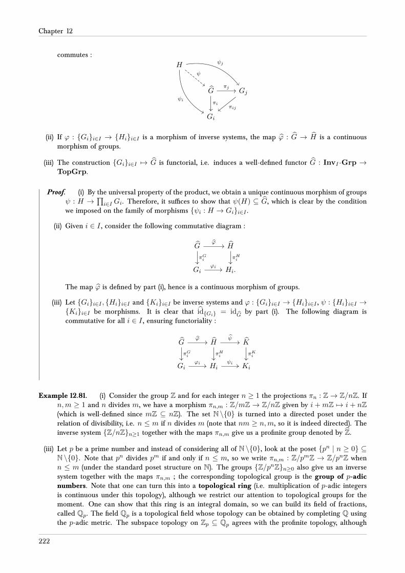
Chapter 12
commutes :H
G Gj
Gi
ψi
ψj
ψ
πj
πiπij
(ii) If ϕ : Gii∈I → Hii∈I is a morphism of inverse systems, the map ϕ : G → H is a continuousmorphism of groups.
(iii) The construction Gii∈I 7→ G is functorial, i.e. induces a well-defined functor G : InvI-Grp →TopGrp.
Proof. (i) By the universal property of the product, we obtain a unique continuous morphism of groupsψ : H →
∏i∈I Gi. Therefore, it suffices to show that ψ(H) ⊆ G, which is clear by the condition
we imposed on the family of morphisms ψi : H → Gii∈I .
(ii) Given i ∈ I , consider the following commutative diagram :
G H
Gi Hi.
ϕ
πGi πHiϕi
The map ϕ is defined by part (i), hence is a continuous morphism of groups.
(iii) Let Gii∈I , Hii∈I and Kii∈I be inverse systems and ϕ : Gii∈I → Hii∈I , ψ : Hii∈I →Kii∈I be morphisms. It is clear that idGi = id
Gby part (i). The following diagram is
commutative for all i ∈ I , ensuring functoriality :
G H K
Gi Hi Ki
ϕ
πGi πHi
ψ
πKiϕi ψi
Example 12.81. (i) Consider the group Z and for each integer n ≥ 1 the projections πn : Z→ Z/nZ. Ifn,m ≥ 1 and n divides m, we have a morphism πn,m : Z/mZ → Z/nZ given by i+mZ 7→ i+ nZ(which is well-defined since mZ ⊆ nZ). The set N \0 is turned into a directed poset under therelation of divisibility, i.e. n ≤ m if n divides m (note that nm ≥ n,m, so it is indeed directed). Theinverse system Z/nZn≥1 together with the maps πn,m give us a profinite group denoted by Z.
(iii) Let p be a prime number and instead of considering all of N \0, look at the poset pn | n ≥ 0 ⊆N \0. Note that pn divides pm if and only if n ≤ m, so we write πn,m : Z/pmZ → Z/pnZ whenn ≤ m (under the standard poset structure on N). The groups Z/pnZn≥0 also give us an inversesystem together with the maps πn,m ; the corresponding topological group is the group of p-adicnumbers. Note that one can turn this into a topological ring (i.e. multiplication of p-adic integersis continuous under this topology), although we restrict our attention to topological groups for themoment. One can show that this ring is an integral domain, so we can build its field of fractions,called Qp. The field Qp is a topological field whose topology can be obtained by completing Q usingthe p-adic metric. The subspace topology on Zp ⊆ Qp agrees with the profinite topology, although
222

Elementary properties of rings and their modules
this leaves the scope of this document, so we omit the details.
(iv) Let K/F be a Galois extension (of possibly infinite degree) and let Gal(K/F ) denote its Galoisgroup. Let F ⊆ E ⊆ K be a subfield such that E/F is a finite Galois extension. The restriction map(−)|E : Gal(K/F ) → Gal(E/F ) has kernel Gal(K/E). One can give a topology on Gal(K/F ),called the Krull topology, by taking the smallest topology for which the cosets of Gal(K/E) inGal(K/F )/Gal(K/E) are open where E ranges over all subfields F ⊆ E ⊆ K for which E/Fis a finite extension. If F ⊆ E1 ⊆ E2 ⊆ K and E1/F , E2/F are finite and Galois extensions,the restriction map gives us morphisms (−)|E1 : Gal(E2/F ) → Gal(E1/F ) and induce an inversesystem Gal(E/F )F⊆E⊆K , giving rise to a profinite group G. By the universal property of G,we can combine the restriction maps (−)|E and obtain a map Gal(K/F ) → G : the fundamentaltheorem of Galois theory implies that this morphism is an isomorphism of topological groups (c.f.Theorem 12.95).
(ii) More generally, let G be an arbitrary group and Nii∈I be a collection of normal subgroups of Gclosed under taking finite intersections (duplicates are allowed). For each i ∈ I , consider the projectionmap πi : G → G/Ni. We turn I into a poset by saying that i ≤ j if Nj ⊆ Ni, which gives us amorphism πij : G/Nj → G/Ni. The collection G/Nii∈I becomes an inverse system and we have amap
G→ G ⊆∏i∈I
G/Ni
with kernel equal to⋂i∈I Ni.
When G = Z and Nnn∈N \0 = nZn∈N \0, we recover Example (i). When we replace nZby pnZ, we recover Example (ii) ; note that in both cases, the map G → G is injective, i.e.⋂n≥1Nn = 0. When G = Gal(K/F ), I is the collection of finite Galois extensions of F in K
and NE = Gal(K/E), if we identify the projection maps Gal(K/F ) → Gal(E/F ) with the projec-tions Gal(K/F ) → Gal(K/F )/Gal(K/E), we recover Example (iii). Note that in this case, we seethat the map Gal(K/F ) → G is injective since a morphism which restricts to the identity on anyfinite Galois subfield of K restricts to the identity (given any α ∈ K , the splitting field of its minimalpolynomial is Galois over F ).
Proposition 12.82. Let Gii∈I be an inverse system and G its inverse limit.
(i) If each Gi is a Hausdorff space, then G is a closed subspace of∏i∈I Gi.
(ii) If each Gi is a compact Hausdorff space, then G is a compact Hausdorff subspace of∏i∈I Gi.
(iii) If each Gi is finite, the profinite group G is compact and Hausdorff.
Proof. (i) The topological group∏i∈I Gi is Hausdorff by Proposition 12.48. Let (gi)i∈I ∈
(∏i∈I Gi
)\
G. By definition of G, there exists i, j ∈ I with i ≤ j such that πij(gj) 6= gi. Let Ui, Uj ⊆ Gi beopen neighborhoods of gi and πij(gj), respectively. It follows that the open set
Ui × π−1ij (Uj)× k ∈ I
k 6=i,jGk
does not intersect G, for if (g′i, g′j) ∈ Ui× π
−1ij (Uj), then πij(g′j) = g′i ∈ Ui implies g′j ∈ π
−1ij (Ui)∩
Uj = ∅. It follows that(∏
i∈I Gi)\ G is open, i.e. G is closed.
(ii) By Tychonoff’s theorem,∏i∈I Gi is compact and it is Hausdorff by Proposition 12.48. Since G is a
closed subspace of∏i∈I Gi, it is a compact Hausdorff subspace.
(iii) Finite sets are compact and Hausdorff as discrete spaces, so we can apply part (ii).
223

Chapter 12
Lemma 12.83. Let Gii∈I be an inverse system such that the maps πij : Gj → Gi are all injective. Thenthe maps πi : G→ Gi are injective.
Proof. Suppose x, y ∈ G ⊆∏i∈I Gi satisfy πi(x) = πi(y). For each j ∈ I , find k ≥ i, j. Then
πj(x) = πjk(πk(x)) = πjk(πk(y)) = πj(y).
It follows that x = (xi)i∈I = (yi)i∈I = y.
Definition 12.84. Let I be a directed poset. A subset J ⊆ I is said to be cofinal if for every i ∈ I , thereexists j ∈ J with i ≤ j.
Proposition 12.85. Let I be a directed poset and J ⊆ I be a cofinal subset.
(i) The poset J is directed.
(ii) Let Gii∈I be an inverse system and consider the inverse system Gjj∈J . There exists a canonicalisomorphism
ΠJ : lim−→j∈J
Gj → lim−→i∈I
Gi.
Proof. (i) If j1, j2 ∈ J , let i ∈ I such that i ≥ j1, j2 (which exists because I is directed). Since J iscofinal, there exists j ∈ I satisfying j1, j2 ≤ i ≤ j, so J is directed.
(ii) Note that this is a general property of inverse limits and cofinal subsets which can be provedcategory-theoretically, but we will prove it directly. The canonical map is defined as follows :choose a function α : I → J such that i ≤ α(i) and j = α(j) for all j ∈ J (via the axiom ofchoice). Then
ΠJ((gj)j∈J)def= (πiα(i)(gα(i)))i∈I .
Injectivity follows from the assumptions that α(j) = j and πii = idGi . For surjectivity, given(gi)i∈I , then ΠJ((gj)j∈J) = (gi)i∈I since if i ∈ I \ J , we have πiα(i)(gα(i)) = gi by definition oflim−→i∈I Gi. It is obviously a continuous morphism of groups by the universal property of the inverselimit, so we are done.
Definition 12.86. Recall the notion of an exact sequence : three groups and two morphisms as displayedin the following diagram
G H Kϕ ψ
is said to be exact at H if kerψ = imϕ. Analogously, it is said to be exact at G if ϕ is injective (i.e. if youpicture the inclusion map 1→ G on the left, kerϕ = im (1→ G)) and exact at K if ψ is surjective (i.e. ifyou picture the projection map K → 1 on the right, imψ = ker(K → 1)). A sequence is said to be exactif it is exact at every group displayed between two other groups in the sequence ; for instance, the abovesequence is called exact if it is exact at H . An exact sequence of the form
1 G H K 1ϕ ψ
is called a short exact sequence.
Proposition 12.87. Let I be a directed poset and ϕ : Gii∈I → Hii∈I , ψ : Hii∈I → Kii∈I be twomorphisms of inverse systems of topological groups. Assume that for each i ∈ I , the sequences
1 Gi Hi Ki 1ϕi ψi
224

Elementary properties of rings and their modules
are short exact sequences. The corresponding sequence
1 G H Kϕ ψ
is exact. Furthermore, if
• the Hi are compact Hausdorff, or
• I = N, the partial order is that of the non-negative integers (i.e. 0 ≤ 1 ≤ 2 ≤ · · · , so thatG0 ⊇ G1 ⊇ G2 ⊇ · · · ), the restriction maps πGij : Gj → Gi are surjective for all i ≤ j and all thetopological groups involved are abelian,
then the sequence
1 G H K 1ϕ ψ
is exact.
Proof. If (gi)i∈I ∈ G satisfies ϕ((gi)i∈I) = 0, then ϕi(gi) = 0 for all i ∈ I , hence gi ∈ kerϕi = 1, i.e.(gi)i∈I = 1, so ϕ is injective. It is clear that ψ ϕ = 0, i.e. im ϕ ⊆ ker ψ. Given (hi)i∈I ∈ ker ψ, wesee that hi = ϕi(gi) for a unique gi ∈ Gi. The injectivity of ϕ ensures that (gi)i∈I ∈ G since we have acommutative square
Gj Hj
Gi Hi.
ϕj
πGij πHij
ϕi
It remains to show that ψ is surjective. First, we use the assumption that the Hi are compact Hausdorff.Let (ki)i∈K ∈ K . For j ∈ J , consider the set
Hj =
(hi)i∈I ∈
∏i∈I
Hi
∣∣∣∣∣ψj(hj) = kj , ∀i ≤ j, πHij (hj) = hi
.
By the surjectivity of the map ψj , the set Hj is non-empty. It is closed as the intersection of the closedsubsets
(πHi )−1(πJij(hj)h−1
i ), i ≤ j and (πKj )−1
(ψj(hj)k−1
j ).
We claim that the sets Hj satisfy the finite intersection property, i.e. that the intersection of finitelymany of them is always non-empty (c.f. Theorem 12.70). Pick j1, · · · , jn ∈ I and choose j ≥ j1, · · · , jntogether with hj ∈ ψ−1
j (kj). For i ≤ j, set hidef= πij(hj) ; for i 6≤ j, choose hi arbitrarily. We claim that
(hi)i∈I ∈⋂nα=1 Hjα . The condition on the hi’s alone is obviously satisfied since i ≤ ji implies i ≤ j and
the morphisms πHij form an inverse system. For 1 ≤ α ≤ n,
ψjα(hjα) = ψjα(πHjαj(hj)) = πKjαj(ψj(hj)) = πKjαj(kj) = kjα .
Since we assume the Hi are compact Hausdorff, H is also compact Hausdorff by Proposition 12.82.Therefore, the intersection ψ−1((ki)i∈I) =
⋂j∈I Hj is non-empty.
Onto the case where the restriction maps in Gi are abelian and the topological groups are abelian(therefore, we denote the operation additively and the neutral element is denoted by 0). Let
G def=∏i∈N
Gi, H def=∏i∈N
Hi, K def=∏i∈N
Ki
225

Chapter 12
and define dG : G → G by dG(gii∈N) = gi − πGij(gj)i∈N. It is clear that ker dG = G. DefinedH : H → H and dK : K → K similarly. By the Snake lemma, the commutative diagram with exact rows
0 G H K 0
0 G H K 0
dG dH dK
leads to the long exact sequence
0 G H K coker dG coker dH coker dK 0.ϕ ψ
so it suffices to show that dG is surjective. Given xii∈N, this means that we have to solve the equations
xi = gi − πGi(i+1)(gi+1), i ∈ N,
which can be done recursively by the surjectivity of πi(i+1) ; the fact that the restriction maps arecompatible with the partial order on I show that if gii∈N is a sequence satisfying the above collectionof equations, then dG(gii∈N) = xii∈N.
12.5 Inverse limits and profinite groups
We first begin by characterizing profinite groups and then prove several topological properties concerningthem.
Lemma 12.88. Let G be a compact topological group and Nii∈I be a family of open normal subgroups(i.e. closed normal subgroups of finite index, c.f. Corollary 12.75) such that for every j1, j2 ∈ I , there
exists i ∈ I such that Ni ⊆ Nj1 ∩ Nj2 . Considering the closed normal subgroup Ndef=⋂i∈I Ni, the
topological groups G/Nii∈I form an inverse system and if G denotes its inverse limit, we have G/N ' Gas topological groups. In particular, if N = 1, then G ' G.
Proof. Define a partial order on I by i ≤ j if and only if Nj ⊆ Ni. The condition on Nii∈Iensures that G/Nii∈I forms an inverse system of topological groups together with the projection mapsπij : G/Nj → G/Ni. By combining the projection maps πi : G → G/Ni, we obtain a continuousmorphism of groups π : G→
∏i∈I G/Ni with kernel N and image being a subset of G. For surjectivity,
let (giNi)i∈I ∈ G. We claim that the sets giNii∈I ⊆ G satisfy the finite intersection property. Giveni1, · · · , ik ∈ I and i0 ∈ I such that Ni0 ⊆
⋂k`=1Ni` , one sees that
πi`ik+1(gik+1
Nik+1) = gi`Ni` , 1 ≤ ` ≤ k =⇒ gik+1
∈k⋂`=1
gi`Ni` .
Therefore, we can pick g ∈⋂i∈I giNi and it follows that π(g) = (gNi)i∈I = (giNi)i∈I , which gives
surjectivity of π. Since G is compact and G is Hausdorff by Proposition 12.82, it follows that π is alsoa closed map (a closed subset of G is compact, thus its image is compact, hence closed in G), hence ahomeomorphism.
Lemma 12.89. Let G be a compact Hausdorff topological group and N ≤ G an open subgroup containingthe subgroup H . The subgroup
NGdef=⋂g∈G
gNg−1
226

Elementary properties of rings and their modules
is an open normal subgroup of G satisfying NGH = HNG ⊆ N . Furthermore, NGH is an open subgroupof G.
Proof. Since conjugation by g ∈ G is a group automorphism of G, we see that NG is normal. The opensubgroup N is of finite index, so if we choose g1, · · · , gn ∈ G such that G/N = g1N, · · · , gnN, we seethat NG =
⋂ni=1 giNg
−1i is open. Normality of NG implies NGH = HNG ⊆ HN = N because H ⊆ N .
The subset NGH is open by Proposition 12.63 and it is a subgroup since NG is normal in G.
Theorem 12.90. Let G be a topological group. The following are equivalent :
(i) The topological group G is a profinite group. More precisely, there exists an inverse system of finitegroups Gii∈I such that G ' G
(ii) The topological group G is compact Hausdorff and 1 ∈ G has a neighborhood basis consisting ofopen normal subgroups
(iii) The topological group G is compact, Hausdorff and totally disconnected (i.e. the only connectedcomponents of G are points).
Proof. ( (i) ⇒ (ii) ) By Proposition 12.82 (iii), G is compact and Hausdorff. Interpreting G as a subgroupof∏i∈I Gi, let Ni E Gi be a normal subgroup for each i ∈ I and J ⊆ I a finite subset. The subgroups
NJ,Nidef= G ∩
∏i∈I\J
Gi
×∏i∈J
Ni
E Gare open normal subgroups of G (by definition of the product and subspace topology). Taking Ni = 1for each i ∈ J show that these NJ,Ni form a neighborhood basis of the identity for the topology of∏i∈I Gi since an open neighborhood of 1 ∈
∏i∈I Gi is the product of open subsets Ui ⊆ Gi where
Ui 6= Gi for only finitely many indices i ∈ I ; for each of those i where Ui 6= Gi, taking Ni = 1 impliesNJ,Ni is contained in that open neighborhood (after that, take intersections with G).
( (ii) ⇒ (iii) ) Let U be the connected component of the identity. By Proposition 12.76, we know thatU is a closed normal subgroup of G and it suffices to show that U = 1. Let Nii∈I be the family
of all open normal subgroups of G and set Uidef= U ∩ Ni. Since Ui is an open normal subgroup of
U , it is closed of finite index by Corollary 12.74, hence U/Ui is finite ; by Proposition 12.76 (iii), wededuce that U ∩ Ni = Ui = U because U is connected, therefore U ⊆ Ni. Since G is Hausdorff,the intersection of all open sets containing 1 is equal to 1, hence U ⊆
⋂i∈I Ni = 1 implies the result.
( (iii) ⇒ (i) ) We first prove that if Nii∈I is the collection of open normal subgroups of G, then⋂i∈I Ni = 1. For g ∈ G \ 1, we show that there exists an open normal subgroup N ⊆ G \ g,
which suffices to complete the argument.
Since G is Hausdorff, there exists an open neighborhood W of 1 not containing g. Let Ukk∈K be thefamily of all clopen neighborhoods of 1. By Theorem 12.78, the assumption that G is totally disconnectedimplies ⋂
k∈KUk = 1.
Since G \W is closed and disjoint from⋂k∈K Uk, the compactness of G gives the existence of a finite
subset K ′ ⊆ K such that(X \W ) ∩
⋂k∈K′
Uk = ∅.
227

Chapter 12
The subset Udef=⋂k∈K′ Uk ⊆ W is a clopen neighborhood of 1 contained in W . For a subset Y ⊆ G,
denote by Y n the set of all products of n elements of Y . Consider
Vdef= (G \ U) ∩ U2.
Since U is compact (because it is closed), U2 = ϕG(U × U) is also compact by Tychonoff’s theorem(where ϕG : G×G→ G is the multiplication map), hence closed ; since G\U is clopen, V is also closed.
For h ∈ U , we claim that there exist open neighborhoods Wh, Xh ⊆ U of h and 1 respectively such thatWhXh ⊆ (G\V )∩U2. To see this, note that G\V ⊆ G is open, hence (h, 1) ∈ (ϕG)−1(G\V ) ⊆ G×Gis an open neighborhood, so it contains a neighborhood of the form W ′h × X ′h since open rectangles
form a basis of the product topology of G × G. Set Whdef= W ′h ∩ U and Xh
def= X ′h ∩ U . It follows that
(h, 1) ∈Wh ×Xh ⊆ U × U , hence h ∈WhXh ⊆ (G \ V ) ∩ U2.
By construction, the collection of all Wh form an open cover of U (because h ∈ U was arbitrary andh ∈ Wh ⊆ U ). Since U is clopen, it is compact, so choose h1, · · · , hn ∈ U with U =
⋃ni=1Whi . Setting
Xdef=⋂ni=1Xhi and Y
def= X ∩X−1 3 1, the subset Y ⊆ X ⊆ U is open and we observe that
UY =n⋃i=1
WhiY ⊆n⋃i=1
WhiXhi ⊆ U.
By induction on n, we have UY n ⊆ U for all n ≥ 1. It follows that Hdef=⋃n≥1 Y
n is an open subgroupof G since
H−1 =
⋃n≥1
Y n
−1
=⋃n≥1
(Y n)−1 =⋃n≥1
(Y −1)n =⋃n≥1
Y n = H
and
HH =
⋃n≥1
Y n
⋃m≥1
Y m
=⋃
n,m≥1
Y n+m = H.
It is contained in U because 1 ∈ U and
H ⊆ UH =⋃n≥1
UY n ⊆⋃n≥1
U = U.
Finally, if we set Ndef= HG (c.f. Lemma 12.89), we have obtained an open normal subgroup
N = HG ⊆ H ⊆ U contained in U .
We have now proven that the family Nii∈I of open normal subgroups of G satisfies⋂i∈I Ni = 1.
It is stable under taking finite intersections, so the set I can be turned into a directed poset by settingi ≤ j if Nj ⊆ Ni. Consider the inverse systems Nii∈I , Gi∈I and G/Nii∈I . In the first case,πNij : Nj → Ni is the inclusion map. In the second case, πGij : G → G is the identity. In the third case,
πG/Nij : G/Nj → G/Ni is the canonical projection. By Proposition 12.87, the exact sequence of inverse
systems
1 Nii∈I Gi∈I G/Nii∈I 1,
defined by the exact sequences 1→ Ni → G→ G/Ni → 1 gives us the following exact sequence :
1 N G G 1.
whereN =⋂i∈I Ni = 1 (we leave this trivial computation to the reader). We deduce that the mapG→ G
is a continuous isomorphism of groups (continuity follows by Proposition 12.80 (ii)). But G is compact
228

Elementary properties of rings and their modules
Hausdorff and the Ni are open normal subgroups, hence closed of finite index by Corollary 12.74. Thismeans that the topological groups G/Ni are finite and discrete, so that G is profinite, and in particularcompact Hausdorff by the implication ( (i) ⇒ (ii) ). Therefore, the map G → G is closed, i.e. anisomorphism of topological groups.
Lemma 12.91. We say that a collection of subsets Sii∈I of a set X is filtered from below if for everyi1, i2 ∈ I , there exists j ∈ I with Sj ⊆ Si1 , Si2 .
Let G be a profinite group and H ≤ G be a closed subgroup.
(i) If Uii∈I is a family of closed subsets filtered from below, then(⋂i∈I
Ui
)H =
⋂i∈I
(UiH).
(ii) Assume H is a closed normal subgroup and that G/H is profinite. If π : G → G/H denotes thecanonical projection and Uii∈I is a family of closed subsets of G filtered from below, then
π
(⋂i∈I
Ui
)=⋂i∈I
π(Ui).
Proof. (i) Since the family Uii∈I is filtered from below, the result is clear if the family is finite sincein this case, there exists i0 ∈ I such that Ui0 ⊆ Ui for all i ∈ I , implying that(⋂
i∈IUi
)H = Ui0H =
⋂i∈I
(Ui0H).
In the general case, it is clear that the inclusion (⊆) holds since⋂i∈I Ui ⊆ Ui0 for any i0 ∈ I
implies(⋂
i∈I Ui)H ⊆ Ui0H , hence the inclusion. For the reverse inclusion, let T ⊆ P(I) (the
power set of I ) be the collection of all finite subsets J ⊆ I . If g ∈⋂i∈I(UiH), then for all J ∈ T ,
g ∈⋂i∈J
UiH =
(⋂i∈J
Ui
)H =⇒ gH ∩
⋂i∈J
Ui 6= ∅.
by our first argument (g = uh with h ∈ H , u ∈⋂i∈J Ui implies gh−1 ∈ gH ∩
⋂i∈J Ui). It follows
that the family of subsetsgH ∩
⋂i∈J
Ui, J ∈ T
satisfies the finite intersection property. Since G is compact and these subsets are closed, thereexists h ∈ H such that
gh ∈⋂J∈T
(gH ∩
⋂i∈J
Ui
)⊆⋂i∈I
Ui =⇒ g ∈
(⋂i∈I
Ui
)H.
(ii) Using part (i), we have
⋂i∈I
π(Ui) =⋂i∈I
UiH/H =
(⋂i∈I
UiH
)/H =
(⋂i∈I
Ui
)H/H = π
(⋂i∈I
Ui
).
229

Chapter 12
Proposition 12.92. Let H be a closed subgroup (resp. closed normal subgroup) of the profinite group G.Then H is the intersection of all the open subgroups (resp. open normal subgroups) of G containing H .
Proof. Recall that open subgroups are closed. If N is an open normal subgroup of G, HN is an opensubgroup of G. Let Nii∈I be the family of open subgroups of G containing H and let N ′jj∈J be thefamily of open normal subgroups of G. By Lemma 12.89, for each open subgroup Ni containing H , the
open normal subgroup N ′jidef= (Ni)G of G satisfies H ⊆ N ′jiH ⊆ Ni, hence Ni = NiH = (N ′jiH)H =
N ′jiH . By applying Lemma 12.91 (i) on the family N ′jj∈J (because open subgroups are closed), we have
⋂i∈I
Ni =⋂i∈I
(N ′jiH)(∗)=⋂j∈J
(N ′jH) =
⋂j∈J
N ′j
H = H.
Note that (∗) holds for the following reason : each (N ′jiH) is of the form N ′jH , so (⊇) is clear.
Covnersely, note that Nidef= N ′jH is an open subgroup of G containing H such that N ′jH = Ni = Nj′i
H ,which implies (⊆). The last equality follows since G is profinite, so the intersection of all its open normalsubgroups is 1. This proves the statement when H is a closed subgroup.
If H is a closed normal subgroup, let Ni be an open subgroup containing H . Then H ⊆ N ′jiH ⊆ Ni
and N ′jiH is normal sincegN ′jiHg
−1 = gN ′jig−1gHg−1 = N ′jiH.
It follows that H equals the intersection of all open subgroups of G containing H by the case we firstdealt with, and also equal to the intersection of all open normal subgroups containing H by the latterargument.
Theorem 12.93. Let G be a profinite group.
(i) If H ≤ G is a closed subgroup, then H is profinite.
(ii) If H ≤ G is a closed normal subgroup, then G/H is profinite.
(iii) If Gii∈I is a family of profinite groups, then∏i∈I Gi is a profinite group.
(iv) If Gii∈I is an inverse system of profinite groups, then G is profinite.
Proof. (i) Given an open normal subgroup Ni ≤ G, the subgroup Hidef= H ∩ Ni is an open normal
subgroup of H . If U is an open subset of H , there exists an open subset V of G satisfyingV ∩ H = U . Since G is profinite, there exists an open normal subgroup Ni of G contained inV , so that Hi ∩ N is contained in U . Clearly H is compact Hausdorff (because G is and H isclosed), so H is compact Hausdorff and its open normal subgroups form a neighborhood basis of1. Therefore, H is profinite by Theorem 12.90.
(ii) Let Nii∈I be the collection of open normal subgroups containing H . We can apply Lemma 12.88to the inverse system G/Nii∈I , so that G ' G/H is profinite by definition (note that G/Ni is afinite Hausdorff topological group by Corollary 12.60, hence discrete).
(iii) Set Gdef=∏i∈I Gi. For each i ∈ I , let Ni E Gi be an open normal subgroup, so that it is closed
of finite index and G/Ni is a finite discrete topological group (as explained in part (ii)). For eachfinite subset J ⊆ I ,
NJ,Nidef=
∏j∈J
Nj
×(∏i∈I\JGi
)E G
230

Elementary properties of rings and their modules
is an open normal subgroup by definition of the product topology since G/NJ,Ni '∏j∈J Gj/Nj
(it is also a finite discrete topological group for the same reasons as before). Letting T be the set ofall finite subsets of I , we have ⋂
J∈TNii∈I
NJ,Ni = 1,
where the intersection is taken over all finite subsets J of I and all possible normal subgroupsNi E Gi. Since G is compact Hausdorff, by Lemma 12.88, we conclude that G ' G is profinite.
(iv) Since G is a closed subgroup of∏i∈I Gi (the restrictions πij(gj)g
−1i = 1 form closed subsets of∏
i∈I Gi for i, j ∈ I with i ≤ j by continuity of multiplication, inversion and the maps πij ), theresult follows by part (i) and (iii).
12.6 Arbitrary Galois extensions and the Krull topology
Recall that given a group G and a collection of normal subgroups of finite index Nii∈I of G partiallyordered under inclusion, we may endow I with a partial order by letting i ≤ j if and only if Nj ⊆ Ni,which gives a canonical morphism of groups πGij : G/Nj → G/Ni. Under the assumption that I isdirected, i.e. that for each i1, i2 ∈ I , there exists i ≤ i1, i2, the collection of groups G/Nii∈I togetherwith the morphisms πGij are a particular case of an inverse system of finite groups. The corresponding
profinite group G ⊆∏i∈I G/Ni comes with a canonical topology coming from the subspace topology of
the product topology, where the groups G/Ni are seen as finite discrete topological groups. This turns G
into a topological group and the canonical map G→ G is surjective with kernel equal to Ndef=⋂i∈I Ni.
Lemma 12.94. Let K/F be a normal extension with structure map ϕ : F → K and set Gdef= Gal(K/F )
(c.f. Definition 12.36 for our convention on the notation Gal). Denote the fixed subfield of G acting on Kby KG.
(i) The field extension K/KG is separable (hence Galois, since it is normal) and the extension KG/F ispurely inseparable.
(ii) The canonical mapKG ⊗F Ksep,F → K, α⊗ β 7→ αβ
is an isomorphism. In particular, K = KGKsep,F is the composite of KG and Ksep,F and theF -subfields KG and Ksep,F are linearly disjoint over F .
(iii) If α ∈ KG \ ϕ(F ), then F is a field of characteristic p and σnp (α) ∈ ϕ(F ) for some n ≥ 1.
(iv) If L is an algebraic closure of F containing K as an F -subfield, then
KGal(K/F ) = KG = K ∩ F p−∞ .
In particular, LAut(L/F ) = F p−∞
.
Proof. In characteristic zero, we have KG = ϕ(F ) and Ksep,F = K , so the result is obvious. Assume weare in characteristic p.
To see that KG/F is purely inseparable, let ψ : KG → L be a morphism of F -fields where Lis an algebraically closed field containing K . Since K/F is normal, K/KG is also normal, sowe can extend this to a morphism of F -fields ψ : K → L. Since the extension K/F is normal,ψ ∈ Aut(K/F ) = Aut(K/KG), meaning that ψ = idKG .
231

Chapter 12
Set Edef= KG. To show that K/KG = K/E is separable, it suffices to show that K ⊗E Ep
−1has
no elements z ∈ K ⊗E Ep−1
satisfying zp = 0 (because zp lies in the image of K under the mapK → K ⊗E Ep
−1, hence it is either a unit or zero). Find x1, · · · , xn ∈ K and y1, · · · , yn ∈ Ep
−1such
that
zdef=
n∑i=1
xi ⊗ yi =⇒ zp =
(n∑i=1
xi ⊗ yi
)p= 0.
Assume n is chosen minimal such that the element z is non-zero. It follows from the minimality that theelements y1, · · · , yn are linearly independent over E. Up to multiplication by x−p1 , we may assume that
x1 = 1. Pick σ ∈ Aut(K/KG) and let σ act on K ⊗E Ep−1
by σ(x ⊗ y)def= σ(x) ⊗ y, which is an
automorphism of E-algebras of K ⊗E Ep−1. It follows that
0 = zp − σ(z)p =
(n∑i=1
xi ⊗ yi
)p−
(n∑i=1
σ(xi)⊗ yi
)p=
(n∑i=2
(xi − σ(xi))⊗ yi
)pBy the minimality of n and the injectivity of the Frobenius endomorphism, we have z = σ(z), hencex1, · · · , xn ∈ KG = E. This gives an E-linear dependence relation between the yi’s, a contradiction. Itfollows that K/KG is separable, hence Galois.
Part (ii) is given by Corollary 12.26. The pure inseparability of KG/F implies part (iii) by definition. Asfor part (iv), the pure inseparability of KG/F implies KG ⊆ K ∩ F p−∞ . Conversely, if α ∈ K satisfiesαp
k ∈ F , then for any σ ∈ G, we have σ(α)pk
= σ(αpk) = αp
k, hence σ(α) = α, which means α ∈ KG.
The particular case of LAut(L/F ) = F p−∞
follows by setting Kdef= L.
Theorem 12.95. Let K/F be a Galois extension and let Eii∈I be the collection of F -subfields of Kwhich are finite Galois extensions of F . (Note that K/Ei is always Galois with Galois group Gal(K/Ei).)
Set Gdef= Gal(K/F ).
(i) For each i ∈ I , the subgroups Gal(K/Ei) ≤ Gal(K/F ) are normal and of finite index. For eachF -subfield Ei of K , the restriction map (−)|Ei : Gal(K/F )→ Emb(Ei/F )K has kernel Gal(K/Ei)and induces the following isomorphism of groups :
Gal(K/F )/Gal(K/Ei) ' Gal(Ei/F ).
More generally, if σ ∈ Gal(K/F ) and E is an arbitrary F -subfield of K , we have σGal(K/E)σ−1 =Gal(K/σ(E)) and restriction to E induces a bijection
Gal(K/F )/Gal(K/E) ' Emb(E/F )K
where Emb(E/F )K denotes the set of morphisms of F -fields E → K . We have Emb(E/F )K =Aut(E/F ) if and only if the extension E/F is Galois, in which case Gal(K/E) is normal (i.e.σ(E) = E for all σ ∈ G) and the above is an isomorphism of groups. Finally, given a subgroupH ≤ Gal(K/F ), the field extension KH/F is Galois if and only if Gal(K/KH) is a normal subgroupof Gal(K/F ).
(ii) Consider the following inverse system of groups. For each Ei, let Gidef= Gal(Ei/F ). Turn I into a
directed set by setting i ≤ j if Ei ⊆ Ej , so that the restriction map πijdef= (−)|EjEi : Gal(Ej/F ) →
Gal(Ei/F ) is a well-defined morphism of groups. We have an isomorphism of groups
Gal(K/F ) ' lim−→i∈I
Gal(Ei/F ), σ 7→ (σ|Ei)i∈I .
One can think of Gal(Ei/F ) as finite discrete groups, which gives lim−→i∈I Gal(Ei/F ) the structureof a profinite topological group. This means the isomorphism of groups endows Gal(K/F ) with a
232

Elementary properties of rings and their modules
profinite topology. Explicitly, the topology of Gal(K/F ) is the coarsest topology such that the leftcosets of the subgroups Gal(K/Ei) ⊆ Gal(K/F ) are clopen. This topology on Gal(K/F ) is calledthe Krull topology.
(iii) Under the Krull topology, Gal(K/F ) is a Hausdorff, compact, totally disconnected topological groupand has a basis of neighborhoods of the identity consisting of open subgroups. (Note that the opensubgroups of Gal(K/F ) are precisely the closed subgroups of finite index ; this is a general propertyof topological groups.) For an F -subfield E ⊆ K , the field extension E/F is finite if and only ifGal(K/E) is an open subgroup of Gal(K/F ).
(iv) (Fundamental theorem of Galois theory, part II) Let H ≤ Gdef= Gal(K/F ) be a subgroup and E be
an F -subfield of K . The correspondence of G-sets
K
subfields Eof K E
containing F
F
←→
1
closed
subgroups H H
of GG
defined by E 7→ Aut(K/E) and H 7→ KH is bijective ; note that we restrict the right-hand side toclosed subgroups of Gal(K/F ). In particular, the closed subgroups of Gal(K/F ) are of the formGal(K/E) where E is an F -subfield of K . Furthermore, we have E = KGal(K/E) for any F -subfieldof K and when E/F is Galois, the isomorphism
Gal(K/F )/Gal(K/E) ' Gal(E/F )
given in part (i) is an isomorphism of topological groups. It follows that given a subgroup H ≤Gal(K/F ), we have
H = Gal(K/KH).
Proof. Without loss of generality, assume all the structure maps of the subfields (including K/F , E/F ,K/E and so on) are given by inclusion maps.
(i) If E/F is a Galois extension where E is an F -subfield of K , an automorphism σ ∈ Gal(K/F )restricts to a map σ|E : E → K satisfying σ(E) = E by Theorem 11.66. It follows thatrestriction (−)|E : Gal(K/F ) → Gal(E/F ) is a morphism of groups with kernel Gal(K/E) bydefinition, and it is surjective by Theorem 11.62. If E = Ei for some i ∈ I , since Gal(Ei/F ) isfinite by definition, Gal(K/Ei) has finite index. The identity σGal(K/E)σ−1 = Gal(K/σ(E))is clear and the fact that restriction to E gives the bijection of sets follows again from Theorem 11.62.
If E/F is Galois, any F -embedding σ : E → K satisfies σ(E) = E, hence σ ∈ Aut(E/F ).Conversely, suppose f(t) ∈ F [t] is an irreducible monic polynomial with a root α ∈ E. ByTheorem 11.62, if β is another root, there exists σ ∈ Gal(K/F ) satisfying σ|E(α) = σ(α) = β ;the assumption σ|E ∈ Aut(E/F ) shows that f(t) splits over E, hence E/F is Galois. Therefore,σ(E) = E for all σ ∈ Gal(K/F ), which means Gal(K/E) E Gal(K/F ) is a normal subgroupand restriction to E gives the desired isomorphism of groups.
For the last statement, it only remains to prove the implication (⇒). Suppose Gal(K/KH) EGal(K/F ) is a normal subgroup. Since Gal(K/F ) permutes roots of irreducible polynomials inF [t] transitively, if f(t) ∈ F [t] has one root in KH , there exists σ ∈ Gal(K/F ) permuting one
233

Chapter 12
root α ∈ KH to another root β ∈ K . But
Gal(K/KH(β)) = Gal(K/σ(KH(α))) = σGal(K/KH)σ−1 = Gal(K/KH) ⊇ H,
which means that β ∈ KH . Therefore, f(t) splits in KH , so that KH/F is a Galois extension.
(ii) Our inverse system is obviously well-defined and the isomorphism of groups in part (i) make acommutative square
Gal(K/F )/Gal(Ej/F ) Gal(Ej/F )
Gal(K/F )/Gal(Ei/F ) Gal(Ei/F ),
'
πij πij
'
giving us an isomorphism of inverse systems Gal(Ei/F )i∈I ' Gal(K/F )/Gal(Ei/F ). Toshow that the corresponding profinite completion of those systems is indeed isomorphic toGal(K/F ), it suffices to see that
⋃i∈I Ei = K and that for any i1, i2 ∈ I , there exists i ∈ I
with Ei1 , Ei2 ⊆ Ei. The first statement is obvious since every α ∈ K is contained in the splittingfield of mα,F (t). For the second, the splitting field of two subsets S1, S2 ⊆ F [t] \ F is containedin the splitting field of S1 ∪ S2. The description of the topology of Gal(K/F ) is the coarsesttopology making the restrictions Gal(K/F ) → Gal(Ei/F ) continuous, so since the latter topo-logical group is discrete, the pre-image of each point σ ∈ Gal(Ei/F ) must be a clopen subsetσGal(K/Ei) ⊆ Gal(K/F ). Note that Gal(K/Ei) E Gal(K/F ) is a normal subgroup, so leftcosets equal right cosets. It follows that U ⊆ Gal(K/F ) is open if and only if it is an arbitraryunion of subsets of the form σi Gal(K/Ei) for some Ei ⊆ K Galois over F and σi ∈ Gal(K/F ).
(iii) The fact that Gal(K/F ) is a Hausdorff compact and totally disconnected topological group to-gether with the statement about its neighborhood basis follows from the fact that it is profinite.Given a finite extension E/F where E is an F -subfield of K , the subgroup Gal(K/E) is open inGal(K/F ) because if L is an E-subfield of K such that L/F is Galois (such as its normal closurein K), each σ ∈ Gal(K/E) has the open neighborhood σGal(K/L) ⊆ Gal(K/E). Conversely,open subgroups H ≤ Gal(K/F ) are closed and of finite index. The core of H , i.e.
H ′def=
⋂σ∈Gal(K/F )
σHσ−1
is also an open subgroup of Gal(K/F ) for the following reason : since H has finitely many leftcosets in Gal(K/F ), after picking a set σ1, · · · , σn of representatives for those cosets, we have
H ′ =n⋂i=1
σiHσ−1i ,
a finite intersection of open subgroups (i.e. an open subgroup again, which is also of finite index).It follows that KH ⊆ KH′ and that KH′ is Galois over F by part (i), so since it has finite index,we have [KH : F ] ≤ [KH′ : F ] <∞, i.e. KH/F is finite.
(iv) We first argue that when E is an F -subfield of K , the subgroup Hdef= Gal(K/E) ≤ Gal(K/F ) is
closed. This follows by the identity
Gal(K/E) =⋂i∈IEi⊆E
[Ei:F ]<∞
Gal(K/Ei).
It holds because E is the union of its subfields which are finite over F , hence Gal(K/Ei) is anopen subgroup (which is closed). Therefore, Gal(K/E) is closed in Gal(K/F ) by definition of the
234

Elementary properties of rings and their modules
Krull topology. Conversely, if H ≤ Gal(K/F ) is closed, then H ⊆ Gal(K/KH). For the reverseinclusion, we will show that H is dense in Gal(K/KH). Suppose σ ∈ Gal(K/KH) and let Lbe a KH-subfield of K such that L/KH is finite and Galois ; it follows that σ admits the openneighborhood σGal(K/L) ⊆ Gal(K/KH). We will show that H ∩ σGal(K/L) 6= ∅. The map
Φ : H → Gal(L/KH), σ 7→ σ|L
is surjective since Φ(H) ≤ Gal(L/KH) is a subgroup of the Galois group of the finite extensionL/KH with fixed field equal to KH (because H ⊆ Gal(K/F ) has fixed field KH and L/KH isGalois), so we can apply the Fundamental theorem of Galois theory, part I. If we choose σ′ ∈ Hsuch that σ′|L = σ|L, we see that σ′ ∈ H ∩ σGal(K/L). Since the open sets σGal(K/L) form abasis for the Krull topology, this shows that H is dense in Gal(K/KH) (which is true regardless ofwhether H is closed or not), so when it is closed, we have H = Gal(K/KH).
235

Chapter 13
Transcendental Field Extensions
13.1 Transcendental extensions
We begin by defining the notion of a dependence relation, which will be recurrent in this chapter (algebraicdependence and p-dependence). Instead of repeating the arguments, we combine everything in one theory,which as a bonus gives us a proof that every vector space has a basis. We assume the reader is minimallyfamiliar with notions of cardinal arithmetic in the case of bases of infinite cardinality.
Definition 13.1. Let A be a set. We will often study relations R ⊆ P(A)× P(A) between subsets of A. Arelation will be denoted by the symbol / in this section. If a ∈ A, we write a / S when a / S.
We call such a relation a dependence relation if it satisfies the following axioms for a ∈ A andS, S′, S′′ ⊆ A :
(i) If T ⊆ S, then T / S
(ii) If a / S, then a / S′ for some finite subset S′ ⊆ S
(iii) (Transitivity) If S / S′ and S′ / S′′, then S / S′′
(iv) (Exchange property) If s ∈ S satisfies a / S and a 6/ S \ s, then s / (S \ s) ∪ a.
(v) (Pointwise property) We have T / S if and only if for all a ∈ T , a / S.
With respect to the dependence relation /, a subset S ⊆ A is called
• dependent if there exists s ∈ S with s / S \ s.
• independent if for any s ∈ S, we have s 6/ S \ s.
• generating if for any a ∈ A, a / S
• a basis if it is independent and generating.
The span of a subset S ⊆ A is defined to be the set of all a ∈ A such that a / S.
Example 13.2. Let V be a vector space over a field K . Write T /S if T ⊆ 〈S〉K , i.e. if T lies in the K-linearspan of S. This is a dependence relation on V ; the independent subsets are the K-linearly independentsubsets and the bases are what they are supposed to be.
Lemma 13.3. Let A be a set with a dependence relation /. Then S ⊆ A is independent if and only if anyfinite subset of S is independent.
236
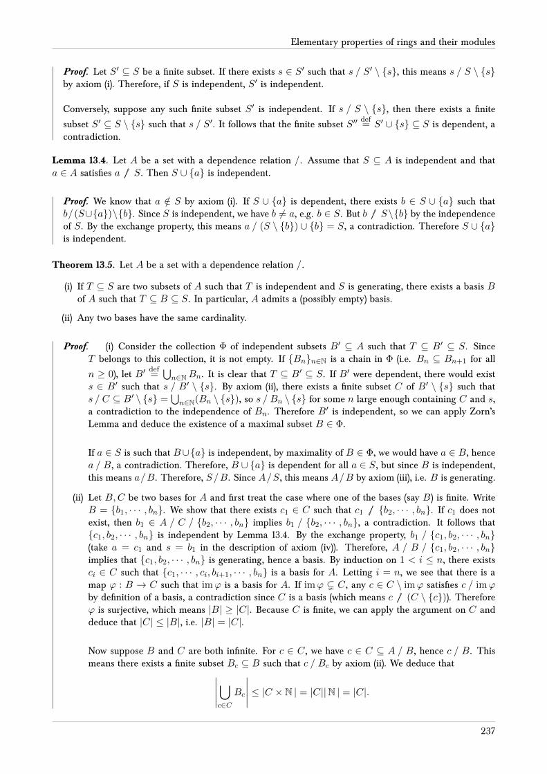
Elementary properties of rings and their modules
Proof. Let S′ ⊆ S be a finite subset. If there exists s ∈ S′ such that s / S′ \ s, this means s / S \ sby axiom (i). Therefore, if S is independent, S′ is independent.
Conversely, suppose any such finite subset S′ is independent. If s / S \ s, then there exists a finite
subset S′ ⊆ S \ s such that s / S′. It follows that the finite subset S′′def= S′ ∪ s ⊆ S is dependent, a
contradiction.
Lemma 13.4. Let A be a set with a dependence relation /. Assume that S ⊆ A is independent and thata ∈ A satisfies a 6/ S. Then S ∪ a is independent.
Proof. We know that a /∈ S by axiom (i). If S ∪ a is dependent, there exists b ∈ S ∪ a such thatb/(S∪a)\b. Since S is independent, we have b 6= a, e.g. b ∈ S. But b 6/ S\b by the independenceof S. By the exchange property, this means a / (S \ b) ∪ b = S, a contradiction. Therefore S ∪ ais independent.
Theorem 13.5. Let A be a set with a dependence relation /.
(i) If T ⊆ S are two subsets of A such that T is independent and S is generating, there exists a basis Bof A such that T ⊆ B ⊆ S. In particular, A admits a (possibly empty) basis.
(ii) Any two bases have the same cardinality.
Proof. (i) Consider the collection Φ of independent subsets B′ ⊆ A such that T ⊆ B′ ⊆ S. SinceT belongs to this collection, it is not empty. If Bnn∈N is a chain in Φ (i.e. Bn ⊆ Bn+1 for all
n ≥ 0), let B′def=⋃n∈NBn. It is clear that T ⊆ B′ ⊆ S. If B′ were dependent, there would exist
s ∈ B′ such that s / B′ \ s. By axiom (ii), there exists a finite subset C of B′ \ s such thats / C ⊆ B′ \ s =
⋃n∈N(Bn \ s), so s / Bn \ s for some n large enough containing C and s,
a contradiction to the independence of Bn. Therefore B′ is independent, so we can apply Zorn’sLemma and deduce the existence of a maximal subset B ∈ Φ.
If a ∈ S is such that B∪a is independent, by maximality of B ∈ Φ, we would have a ∈ B, hencea / B, a contradiction. Therefore, B ∪ a is dependent for all a ∈ S, but since B is independent,this means a/B. Therefore, S/B. Since A/S, this means A/B by axiom (iii), i.e. B is generating.
(ii) Let B,C be two bases for A and first treat the case where one of the bases (say B) is finite. WriteB = b1, · · · , bn. We show that there exists c1 ∈ C such that c1 6 / b2, · · · , bn. If c1 does notexist, then b1 ∈ A / C / b2, · · · , bn implies b1 / b2, · · · , bn, a contradiction. It follows thatc1, b2, · · · , bn is independent by Lemma 13.4. By the exchange property, b1 / c1, b2, · · · , bn(take a = c1 and s = b1 in the description of axiom (iv)). Therefore, A / B / c1, b2, · · · , bnimplies that c1, b2, · · · , bn is generating, hence a basis. By induction on 1 < i ≤ n, there existsci ∈ C such that c1, · · · , ci, bi+1, · · · , bn is a basis for A. Letting i = n, we see that there is amap ϕ : B → C such that imϕ is a basis for A. If imϕ ( C , any c ∈ C \ imϕ satisfies c / imϕby definition of a basis, a contradiction since C is a basis (which means c 6/ (C \ c)). Thereforeϕ is surjective, which means |B| ≥ |C|. Because C is finite, we can apply the argument on C anddeduce that |C| ≤ |B|, i.e. |B| = |C|.
Now suppose B and C are both infinite. For c ∈ C , we have c ∈ C ⊆ A / B, hence c / B. Thismeans there exists a finite subset Bc ⊆ B such that c / Bc by axiom (ii). We deduce that∣∣∣∣∣⋃
c∈CBc
∣∣∣∣∣ ≤ |C × N | = |C||N | = |C|.237

Chapter 13
If we can show that⋃c∈C Bc = B, we will have finished the proof by symmetry and the Cantor-
Schröder-Bernstein theorem. One inclusion (⊆) is clear. For the reverse inclusion (⊇), if b ∈B \
⋃c∈C Bc, we have
b / A / C /⋃c∈C
Bc ⊆ B \ b,
a contradiction to the independence of B.
We now turn to the study of transcendental extensions.
Definition 13.6. Let K/F be a field extension and S ⊆ K a subset. Recall that F (S) ⊆ K is the smallestF -subfield of K containing S, which can be obtained as follows : the polynomial map
F [xss∈S ]→ K, xs 7→ s ∈ K
has a kernel, say p E F [xss∈S ]. The quotient map F [xss∈S ]/p → K is a map of integral domains, sogives an injection Q(F [xss∈S ]/p)→ K of the field of fractions with image F (S). The image can be de-scribed as the set of all fractions f(s1,··· ,sn)
g(s1,··· ,sn) where f, g ∈ F [xss∈S ], s1, · · · , sn ∈ S and g(s1, · · · , sn) 6= 0.
We say that a ∈ K is algebraically dependent of S over F if the field extension F (S ∪ a)/F (S) isalgebraic. Equivalently, a is algebraically dependent of S if there exists s1, · · · , sn ∈ S and a polynomialf ∈ F [S][t] such that f(s1, · · · , sn, a) = 0 and degt f > 0 when seeing f as a polynomial in the singlevariable t (i.e. the variable t appears in the expression, this is what the subscript in degt stands for) andF [S] ⊆ K is the F -subalgebra of K generated by S (the difference between the two definitions lies inclearing/adding denominators). Such a polynomial f ∈ F [S][t] is called a polynomial relation for a overS (or simply a polynomial relation between those elements).
A subset T ⊆ K is algebraically dependent of S over F if the field extension F (S ∪ T )/F (S) isalgebraic.
Theorem 13.7. Let K/F be a field extension. The relation T / S defined by “T is algebraically dependentof S over F ” is a dependence relation on K which corresponds to the relation “a is algebraically dependntof S over F ” defined for elements when T is a singleton.
Proof. We prove that each of the axioms of Definition 13.1 hold.
(i) If T ⊆ S, then F (S ∪ T ) = F (S) is algebraic over F (S), so T / S.
(ii) If a / S, there exists a polynomial equation f(s1, · · · , sn, a) = 0 where f(x1, · · · , xn, t) ∈F [x1, · · · , xn][t], s1, · · · , sn ∈ S and degt f > 0. letting S′
def= s1, · · · , sn, we see that a / S′.
(iii) If the extensions F (S ∪S′)/F (S) and F (S′∪S′′)/F (S′) are algebraic, we show that the extensionF (S ∪ S′ ∪ S′′)/F (S) is algebraic. By assumption, the subsets S′ ∪ S′′ is algebraic over F (S′),hence also over F (S∪S′′). The subset S is clearly algebraic over F (S), hence also over F (S∪S′).This means that F (S ∪ S′ ∪ S′′)/F (S ∪ S′′) is generated by algebraic elements, thus algebraic.Since F (S ∪S′′)/F (S) is also algebraic, we conclude by Theorem 11.39 that F (S ∪S′ ∪S′′)/F (S)is algebraic, and in particular F (S ∪ S′′)/F (S) is algebraic.
(iv) If a / S and a 6 / S \ s, this means that a polynomial relation f(s1, · · · , sn, s, a) = 0 wheref ∈ F [x1, · · · , xn, x, t] with degt f > 0 must satisfy degx f > 0. By definition, the existence ofthis relation implies s / (S \ s) ∪ a.
(v) It is clear that F (S ∪ T )/F (S) is algebraic if and only if each a ∈ T is algebraic over F (S), i.e.T / S if and only if a / S for all a ∈ T .
238

Elementary properties of rings and their modules
Definition 13.8. Let K/F be a field extension and a ∈ K , S ⊆ K . With respect to the relationship ofalgebraic dependence, the subset S is said to be
(i) algebraically dependent over F if it is dependent, i.e. if there exists a polynomial f ∈ F [xss∈S ]\F with f(s1, · · · , sn) = 0 for some s1, · · · , sn ∈ S
(ii) algebraically independent over F if it is independent, i.e. there exists no polynomial f ∈ F [xss∈S ]\F with f(s1, · · · , sn) = 0 for some s1, · · · , sn ∈ S
(iii) algebraically generating the extension K/F if K/F (S) is algebraic, i.e. if K = Kalg,F (S)
(iv) completely generating the extension K/F if K = F (S) (this is new from the abstract theory ofdependence relations, since as we can see from part (iii) of the definition, the abstract theory onlygives K = Kalg,F (S) and not K = F (S))
(v) a transcendence basis if it is a basis, i.e. S is algebraically independent over F and K/F (S) isalgebraic.
The cardinality of a transcendence basis is called the transcendence degree of the extension K/F and isdenoted by tr.deg(K/F ).
An element a ∈ K is said to be transcendental over F if it is not algebraic, i.e. if a is algebraicallyindependent over F (or in other words, if a / ∅). The field extension K/F is called transcendental if it isnot algebraic, i.e. if it contains at least one transcendental element. It will often be convenient to deal withfamilies of elements instead of subsets. A family aii∈I of distinct elements ofK is said to be algebraicallydependent (resp. independent) if there exists a polynomial relation (resp. no polynomial relation) of theform f(ai1 , · · · , ain) = 0 for f ∈ F [x1, · · · , xn] \ F and i1, · · · , in ∈ I . (A family of non-distinct elementsof K is automatically considered algebraically dependent.)
If S is algebraically independent and completely generates the extension K/F (so that K = F (S) whereS is a transcendence basis), we say that the extension K/F is purely transcendental.
Remark 13.9. (i) If K/F is a field extension, the subset S ⊆ K is algebraically independent over F ifand only if the set
n∏i=1
si11 · · · sinn
∣∣∣∣∣n, i1, · · · , in ≥ 0, s1, · · · , sn ∈ S
is F -linearly independent (an F -linear dependence relation is equivalent to a polynomial equation).In particular, s ∈ K is algebraically independent if and only if the set 1, s, · · · , sn, · · · is F -linearlyindependent, i.e. no polynomial f ∈ F [t] satisfies f(s) = 0.
(ii) It is clear that if E/K and K/F are two field extensions, the field extension E/F is transcendental ifand only if E/K or K/F is transcendental.
Corollary 13.10. Let K/F be a field extension. The following are equivalent :
(i) The subset S ⊆ K is algebraically independent over F
(ii) The map of F -algebras F [xss∈S ]→ K defined by xs 7→ s is injective
(iii) For every s ∈ S, the element s is transcendental over F (S \ s).
239

Chapter 13
Proof. Saying that there are no polynomial relations between the elements of S is equivalent to sayingthat the map in part (ii) has trivial kernel, which gives the equivalence of part (i) and part (ii). Equivalenceof part (i) and part (iii) follows by the definition of the dependence relation / since a polynomial relationf(s1, · · · , sn) = 0 implies that si / s1, · · · , si−1, si+1, · · · , sn for some 1 ≤ i ≤ n, i.e. si / S \ si.
Corollary 13.11. If K/F is a purely transcendental extension with transcendence basis S, the map
Q(F [xss∈S ])→ K, xs 7→ s
is an isomorphism of F -fields. In particular, any two purely transcendental extensions of the same tran-scendence degree are isomorphic.
Proof. For the first statement, the fact that S is a transcendence basis shows that the map is injective ;by assumption that K/F is purely transcendental, it is surjective. For the second statement, if S and Tare two transcendence bases for F (S)/F and F (T )/F , a bijection S → T lifts to an isomorphism ofF -fields
F (S) ' Q(F [xss∈S ] ' Q(F [xtt∈T ] ' F (T ).
Corollary 13.12. Let K/F be a field extension.
(i) The field K has a transcendence basis over F and any two transcendence bases have the samecardinality, so the transcendence degree tr.deg(K/F ) is well-defined.
(ii) If T ⊆ K is algebraically independent over F , there exists a transcendence basis S of K over Fcontaining T .
(iii) If S ⊆ K is a subset such that K/F (S) is algebraic, then S contains a transcendence basis for Kover F .
Proof. This follows from Theorem 13.5.
Proposition 13.13. Let K/F and E/K be field extensions where the structure map of E/K is given byinclusion, S1 is a transcendence basis for K over F and S2 is a transcendence basis for E over K . ThenS1 ∪ S2 is a transcendence basis for E/F and
tr.deg(E/F ) = tr.deg(E/K) + tr.deg(K/F ).
Proof. We first prove that S1 ∪ S2 is a transcendence basis for E over F .
Since S2 is algebraically independent over K ⊇ F (S1), it is clear that S1 ∪ S2 is algebraicallyindependent since a polynomial relation between those elements either implies a polynomial relationfor elements of S2 over K (if one element of S2 is involved in the relation) or a polynomial relation ofelements of S1 over F (if no element of S2 is involved in the relation), which doesn’t exist in any case.
The extensionsK/F (S1) and E/K(S2) are algebraic. SinceK is algebraic over F (S1) ⊆ F (S1∪S2) andS2 is trivially algebraic over F (S1 ∪ S2), we see that K(S2)/F (S1 ∪ S2) is algebraic. Since E/K(S2) isalso algebraic, this means that E/F (S1∪S2) is algebraic by Theorem 11.39, i.e. S1∪S2 is a transcendencebase for E. Since S1 ∩ S2 = ∅ by the fact that S2 is algebraically independent over K ⊇ F (S1), we seethat |S1 ∪ S2| = |S1|+ |S2|.
Proposition 13.14. Let E/F be a field extension and K1,K2 ⊆ E be two F -subfields. Then
tr.deg(K1K2/K1) ≤ tr.deg(K2/F ), tr.deg(K1K2/F ) ≤ tr.deg(K1/F ) + tr.deg(K2/F ).
240

Elementary properties of rings and their modules
Proof. Let S be a transcendence basis for K2 over F , so that K2/F (S) is algebraic. SinceK1K2 = K1(K2), it follows that K1K2/K1(S) is an algebraic extension since the elements of K2 arealgebraic over K1(S) ⊇ F (S). Therefore, we can find a transcendence basis T ⊆ S for K1K2 over K1
by Corollary 13.12, which gives the first inequality.
For the second inequality, note that by the first inequality applied to K2 instead of K1, we have
tr.deg(K1K2/F ) = tr.deg(K1K2/K2) + tr.deg(K2/F ) ≤ tr.deg(K1/F ) + tr.deg(K2/F ).
Lemma 13.15. Let E/K and K/F be field extensions. Any σ ∈ Aut(K/F ) equals the restriction of someσ ∈ Aut(E/F ) to K .
Proof. If S is a transcendence basis for E/K , F -automorphisms of K lift to F -automorphisms ofK(S) via an arbitrary function S → K(S) by Theorem 1.56 and Theorem 8.4, which then lift to F -automorphisms of E by Theorem 11.62.
Theorem 13.16. Let Ω/F be a field extension where Ω is algebraically closed (so that F p−∞ ⊆ Ω in the
case where ch(F ) = p). Then
ΩAut(Ω/F ) =
F p−∞
if ch(F ) = p > 0
F if ch(F ) = 0.
Proof. We first show that tr.deg(ΩAut(Ω/F )/F ) = 0. Let S be a transcendence basis for ΩAut(Ω/F ) overF and T be a transcendence basis for Ω over ΩAut(Ω/F ). Since S ∪ T is a transcendence basis for Ωover F , any permutation of S1 ∪ S2 gives rise to an F -automorphism of F (S), which then lifts to anelement of Aut(Ω/F ) and therefore, this permutation has to fix S1 ⊆ ΩAut(Ω/F ). This implies eitherS1 = ∅ or (S1, S2) = (s,∅). The second case is contradictory because non-trivial automorphisms ofF (s) over F lift to automorphisms of Ω over F which are not trivial (there are as many as |F (s) \ F |such automorphisms).
Set Edef= ΩAut(Ω/F ) and let α ∈ E. For σ ∈ Aut(E/F ), find a lift σ ∈ Aut(Ω/F ). Since σ(α) =
σ(α) = α, we see that α ∈ EAut(E/F ). Let K ⊆ Ω be an algebraic closure for F ; since E/F is algebraic,E ⊆ K . It is also clear that E ⊆ KAut(K/F ) since F -automorphisms of K lift to F -automorphisms ofΩ, so by Lemma 12.94 (iv), when ch(F ) = 0, we get E ⊆ F . When ch(F ) = p > 0, we get E ⊆ F p
−∞.
Since automorphisms in Aut(Ω/F ) have to fix K (because they fix F , hence permute algebraic elementswithin the set of roots of their minimal polynomials), we have F p
−∞= KAut(K/F ) ⊆ E, which implies
E = F p−∞
.
Definition 13.17. A field extension K/F is said to be finitely generated if K = F (S) for a finite subsetS ⊆ K .
Lemma 13.18. If K/F is a finitely generated field extension and S is a transcendency basis for K over F ,then S is finite and K/F (S) is a finite extension.
Proof. By hypothesis, there exists a finite subset T ⊆ K such that K = F (T ), hence it contains atranscendence basis for K over F , which must be finite. It follows that tr.deg(K/F ) <∞. If S ⊆ K is atranscendence basis, then K = F (S ∪ T )/F (S) is generated by finitely many algebraic elements, henceis finite by Theorem 11.36.
241

Chapter 13
Proposition 13.19. Let E/F be a finitely generated field extension and K ⊆ E be an F -subfield. Theextension K/F is finitely generated and tr.deg(K/F ) ≤ tr.deg(E/F ) with equality if and only if E/K isalgebraic.
Proof. By Proposition 13.13, we know that tr.deg(K/F ) ≤ tr(E/F ) < ∞ with equality if and onlyif tr.deg(E/K) = 0, i.e. if and only if E/K is algebraic. It remains to show thatK/F is finitely generated
First deal with the case where tr.deg(K/F ) = 0, i.e. when K/F is algebraic. If y1, · · · , yr is anF -basis for K , we claim that they are linearly independent over F (x1, · · · , xn) where x1, · · · , xn is atranscendence basis for E/F . To see this, suppose we have a linear relation of the form
r∑i=1
fi(x1, · · · , xn)yi = 0, f1, · · · , fr ∈ F [x1, · · · , xn].
This is a polynomial in K[x1, · · · , xn] whose coefficient in front of each monomial in the variablesx1, · · · , xn is a linear relation between the elements y1, · · · , yr over F , hence all its coefficients have tobe zero. This means the f1, · · · , fr are equal to zero, proving the claim. Therefore,
[K : F ] ≤ [E : F (x1, · · · , xn)] <∞.
Onto the general case. Let T be a transcendence basis for K over F , which is finite. Since E is finitelygenerated over F , it is also finitely generated over F (T ). The extension K/F (T ) is algebraic, hencefinitely generated by the algebraic case ; this means K/F is also finitely generated.
Proposition 13.20. Let K/F be a purely transcendental extension with structure map ϕ : F → K . ThenKalg,F = ϕ(F ).
Proof. Without loss of generality, assume that ϕ is the inclusion map. Let S ⊆ K be a transcendencebasis such that K = F (S). Since any element x ∈ K is contained in F (Sx) where Sx ⊆ S is a finitesubset of S, we may assume that S = s1, · · · , sn is finite and proceed by induction on n.
For n = 1, let x ∈ F (s) be algebraic over F . Writing x = f(s)/g(s) for some polynomials f, g ∈ F [t]with g(s) 6= 0 and f(t), g(t) have no common factor, we see that xg(s) − f(s) = 0. If x ∈ F (s) \ F ,then s is algebraic over F (x). By assumption, F (x)/F is algebraic, which means s is algebraic over F , acontradiction. Therefore x ∈ F and F (s)alg,F = F .
For n > 1, suppose that x ∈ F (s1, · · · , sn) is algebraic over F , hence algebraic over F (s1, · · · , sn−1).By the cases where n is replaced by 1 and n− 1, we see that x ∈ F (s1, · · · , sn−1)alg,F = F .
Proposition 13.21. Let E/F be a field extension and K ⊆ E be an F -subfield. Suppose that S ⊆ E isalgebraically independent over K (and therefore also over F ). The extension K(T )/F (T ) is algebraic ifand only if K/F is algebraic.
Proof. It is clear that if K/F is algebraic, then so is K(T )/F (T ) since K and T are algebraic overF (T ). Conversely, suppose K(T )/F (T ) is algebraic. It follows that T is a transcendence basis for K(T )over F since it is linearly independent and K(T )/F (T ) is algebraic by assumption. On the other hand,considering the extensions K(T )/K and K/F , we have
tr.deg(K(T )/F ) = tr.deg(K(T )/K) + tr.deg(K/F ) = tr.deg(K(T )/F ) + tr.deg(K/F )
which implies that tr.deg(K/F ) = 0, so that K/F is algebraic.
242
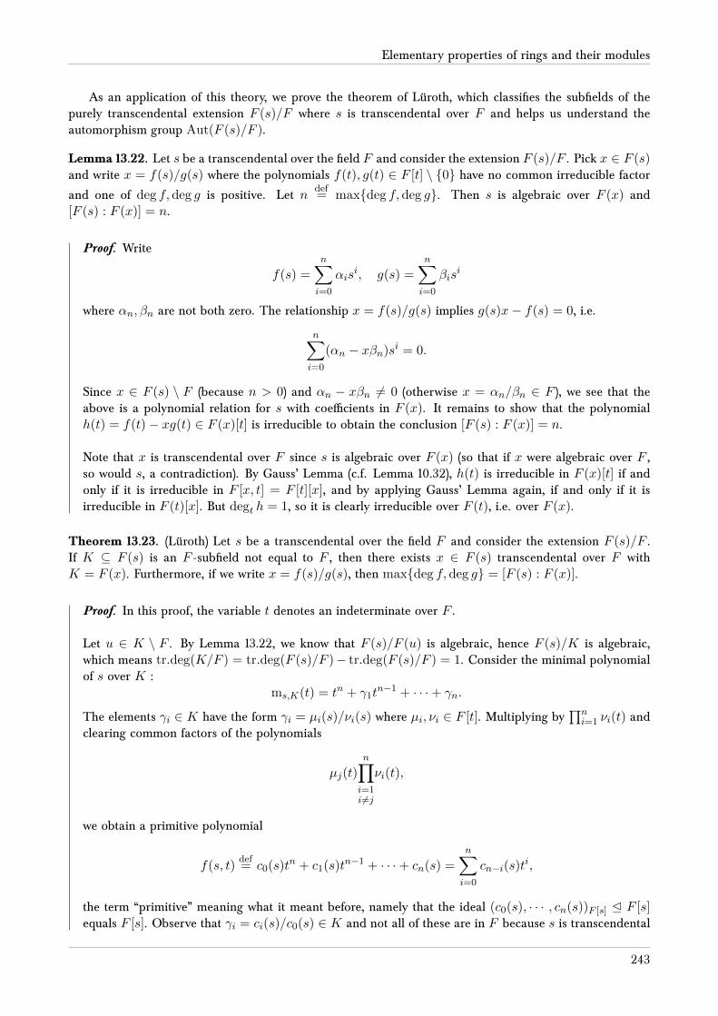
Elementary properties of rings and their modules
As an application of this theory, we prove the theorem of Lüroth, which classifies the subfields of thepurely transcendental extension F (s)/F where s is transcendental over F and helps us understand theautomorphism group Aut(F (s)/F ).
Lemma 13.22. Let s be a transcendental over the field F and consider the extension F (s)/F . Pick x ∈ F (s)and write x = f(s)/g(s) where the polynomials f(t), g(t) ∈ F [t] \ 0 have no common irreducible factor
and one of deg f,deg g is positive. Let ndef= maxdeg f,deg g. Then s is algebraic over F (x) and
[F (s) : F (x)] = n.
Proof. Write
f(s) =
n∑i=0
αisi, g(s) =
n∑i=0
βisi
where αn, βn are not both zero. The relationship x = f(s)/g(s) implies g(s)x− f(s) = 0, i.e.
n∑i=0
(αn − xβn)si = 0.
Since x ∈ F (s) \ F (because n > 0) and αn − xβn 6= 0 (otherwise x = αn/βn ∈ F ), we see that theabove is a polynomial relation for s with coefficients in F (x). It remains to show that the polynomialh(t) = f(t)− xg(t) ∈ F (x)[t] is irreducible to obtain the conclusion [F (s) : F (x)] = n.
Note that x is transcendental over F since s is algebraic over F (x) (so that if x were algebraic over F ,so would s, a contradiction). By Gauss’ Lemma (c.f. Lemma 10.32), h(t) is irreducible in F (x)[t] if andonly if it is irreducible in F [x, t] = F [t][x], and by applying Gauss’ Lemma again, if and only if it isirreducible in F (t)[x]. But degt h = 1, so it is clearly irreducible over F (t), i.e. over F (x).
Theorem 13.23. (Lüroth) Let s be a transcendental over the field F and consider the extension F (s)/F .If K ⊆ F (s) is an F -subfield not equal to F , then there exists x ∈ F (s) transcendental over F withK = F (x). Furthermore, if we write x = f(s)/g(s), then maxdeg f, deg g = [F (s) : F (x)].
Proof. In this proof, the variable t denotes an indeterminate over F .
Let u ∈ K \ F . By Lemma 13.22, we know that F (s)/F (u) is algebraic, hence F (s)/K is algebraic,which means tr.deg(K/F ) = tr.deg(F (s)/F )− tr.deg(F (s)/F ) = 1. Consider the minimal polynomialof s over K :
ms,K(t) = tn + γ1tn−1 + · · ·+ γn.
The elements γi ∈ K have the form γi = µi(s)/νi(s) where µi, νi ∈ F [t]. Multiplying by∏ni=1 νi(t) and
clearing common factors of the polynomials
µj(t)n∏i=1i 6=j
νi(t),
we obtain a primitive polynomial
f(s, t)def= c0(s)tn + c1(s)tn−1 + · · ·+ cn(s) =
n∑i=0
cn−i(s)ti,
the term “primitive” meaning what it meant before, namely that the ideal (c0(s), · · · , cn(s))F [s] E F [s]equals F [s]. Observe that γi = ci(s)/c0(s) ∈ K and not all of these are in F because s is transcendental
243

Chapter 13
over F . It follows that one of them has the form γdef= γi = g(s)/h(s) where g, h ∈ F [t] have no common
factor and maxdeg g,deg h = m > 0. By Lemma 13.22, we know that g(t) − γh(t) is irreducible inF (γ)[t] and [F (s) : F (γ)] = m. The fact that K ⊇ F (γ) and [F (s) : K] = n implies m ≥ n. It remainsto show that m = n, which will imply K = F (γ), as desired.
Since s is a root of g(t)− γh(t) ∈ K[t], we see that ms,K(t) divides g(t)− γh(t) in K[t]. Write
g(t)− γh(t) = ms,K(t)q(t), q(t) ∈ K[t].
Since γ = g(s)/h(s), we may substitute in the above and multiply by h(s) to obtain the relationship
g(t)h(s)− g(s)h(t) = ms,K(t)q(t)h(s)
in K[t]. Since K ⊆ F (s), by multiplying by an appropriate factor k(s) ∈ F [s], we obtain a polynomialrelation in F [s, t] :
(g(t)h(s)− g(s)h(t))k(s) = f(s, t)q(s, t).
(To proceed, obtain f(s, t) by multiplying by the appropriate denominator and clearing multiple factorsas when we constructed f(s, t) earlier and give the remaining factors to q(t) to obtain q(s, t).)
Since f(s, t) is primitive, it follows that k(s) divides q(s, t), so we might assume without loss of generalitythat k(s) = 1. In the equation
g(t)h(s)− g(s)h(t) = f(s, t)q(s, t),
we see that degs h(s)g(t) − g(s)h(t) ≤ maxdeg g,deg h = m. Since g(s) and h(s) have no commonfactor, it follows that c0(s) = h(s) and ci(s) = g(s). The equality maxdeg g,deg h = m then implies
degs f(s, t) ≥ maxdegs c0(s), degs ci(s) = maxdegs g(s),degs h(s) = m.
It follows that degs f(s, t) = m = degs g(t)h(s) − g(s)h(t). This implies that degs q(s, t) = 0, i.e.q(s, t) = q(t) ∈ F [t]. This means that the polynomial on the right-hand side is a primitive polynomialin s. This is also true of the right-hand side, but by symmetry, the left-hand side is also a primitivepolynomial in t. It follows that f(s, t)q(t) is a primitive polynomial in t, hence q(t) ∈ F . Therefore,degs f(s, t) = degt f(s, t), which implies
[F (s) : F (γ)] = maxdeg g,deg h = m = degs f(s, t) = degt f(s, t) = n = [F (s) : K].
Corollary 13.24. Let s be transcendental over the field F .
(i) For all 2× 2 matrices[α βγ δ
]∈ GL2(F ), the map
s 7→ αs+ β
γs+ δ
determines a unique F -automorphism of F (s).
(ii) The map GL2(F )→ Aut(F (s)/F ) defined by part (i) is a surjective morphism of groups with kernelconsisting of all F -multiples of the identity matrix. In particular,
Aut(F (s)/F ) ' PGL2(F ),
the projective linear group of 2× 2 matrices over F (defined precisely as this quotient of GL2(F ) bythe normal subgroup of F -multiples of the identity matrix).
244

Elementary properties of rings and their modules
Proof. An F -endomorphism of F (s) has to be defined by sending s to a rational polynomial f(s)g(s) . By
Theorem 13.23, it can only be an automorphism if maxdeg f,deg g = 1, i.e. if it is a ratio of twopolynomials of degree ≤ 1 with no common factor, which is the claim. Note that to check this claim, onemust see that if αδ − βγ = 0, f(s)/g(s) ∈ F (if it is not zero, we will prove in the proof of part (ii) thatf(s)/g(s) ∈ F (s) \ F ).
Let[α1 β1
γ1 δ1
],
[α2 β2
γ2 δ2
]∈ GL2(F ) be two matrices with non-zero determinant. It follows by clearing
denominators thatα1
(α2s+β2
γ2s+δ2
)+ β1
γ1
(α2s+β2
γ2s+δ2
)+ δ1
=(α1α2 + β1γ2)s+ (α1β2 + β1δ2)
(γ1α2 + δ1γ2)s+ (γ1β2 + δ1γ2)
shows that the map GL2(F ) → Aut(F (s)/F ) is a morphism of groups. It also shows that when
det
([α βγ δ
])6= 0, αs+β
γs+δ ∈ F (s) \ F ; otherwise we couldn’t map this element back to s via an
F -automorphism of F (s). The surjectivity of GL2(F ) → Aut(F (s)/F ) follows by Theorem 13.23, and
its kernel can be computed by looking at all the matrices[α βγ δ
]∈ GL2(F ) such that αs+β
γs+δ = s. It is
clear that γ = 0 by clearing denominators and comparing degrees. Comparing terms, we see that β = 0and α/δ = 1, which is the result.
Remark 13.25. It is a theorem of Castelnuovo that if K/F is a purely transcendental extension of tran-scendence degree 2, then any F -subfield of K of transcendence degree 2 is again purely transcendental.However, the author is not aware of a proof at the moment.
13.2 Separable extensions
Let F be a field of characteristic p ≥ 0 and let L be an algebraically closed field containing F . If p > 0
and n > 1, we have defined the subfields F p−n def
= σ−np (F ) ⊆ L and we had found a perfect closure of F
sitting inside L, namely F p−∞ def
=⋃n≥1 F
p−n . The main part of this chapter is to characterize separability
via tensor products and the fields F p−1, F p
−nand F p
−∞.
Definition 13.26. Let K/F be a field extension and let L be an algebraic closure for K . We say that K/Fis separable if K and F p
−1are linearly disjoint subfields of L over F (c.f. Definition 11.44). If p = 0 or if
p > 0 and F is perfect, we have F p−1
= F , hence every field extension K/F is separable ; this generalizesCorollary 12.27 to arbitrary extensions and is compatible with the definition of separability in the algebraiccase by Theorem 12.25.
A transcendence basis S for K/F such that K/F (S) is separably algebraic is called a separatingtranscendence basis. A field extension K/F which admits such a transcendence basis is called separablygenerated.
Lemma 13.27. Let E/K and K/F be two field extensions. If S ⊆ E is algebraically independent over K ,then K and F (S) are linearly disjoint over F .
Proof. It is clear that K and F (S) are linearly disjoint over F if and only if K and F [S] are linearly dis-joint over F (just clear denominators). Since S is algebraically independent over F , the set of monomialsin elements of S is F -linearly independent, hence the map
K ⊗F F [S]→ E
245

Chapter 13
is an isomorphism onto K[S], which means that K and F [S] are linearly disjoint over F , completing theproof.
Corollary 13.28. Any purely transcendental extension is separable and separably generated.
Proof. Let K/F be a purely transcendental extension and choose a transcendence basis S ⊆ K , sothat K = F (S). The subset S ⊆ Kp−1
is obviously algebraically independent over F p−1
since iff(s1, · · · , sn) = 0 is a polynomial relation over F p
−1, its pth power is a polynomial relation over F , a
contradiction. It follows that F (S) and F p−1
are linearly disjoint over F by Lemma 13.27, i.e. K = F (S)is separable over F .
The extension F (S)/F is clearly separably generated with separating transcendence basis S sinceF (S)/F (S) is separably algebraic.
Proposition 13.29. Let K/F and E/K be two field extensions.
(i) If E/F is separable, then so is K/F .
(ii) If K/F and E/K are separable, then so is E/F .
(iii) If K/F is separably generated and E/K is separably algebraic, then E/F is separably generated.
Proof. (i) This is clear since the linear disjointness of E and F p−1
implies that of K and F p−1.
(ii) Let S ⊆ F p−1
be a subset of F -linearly independent elements. Since K and F p−1
are linearlydisjoint, the subset S ⊆ Kp−1
is K-linearly independent. It follows that it is also an E-linearlyindependent subset of Ep
−1since E and Kp−1
are linearly disjoint over K . This means that E andF p−1
are linearly disjoint over F , i.e. E/F is separable.
(iii) Let S be a separating transcendence basis forK/F . It follows thatK/F (S) and E/K are separablyalgebraic, so E/F (S) is separably algebraic by Proposition 12.14 ; this implies that S is a separatingtranscendence basis for E/F , i.e. E/F is separably generated.
Remark 13.30. Let E/K and K/F be two field extensions. The separability of E/F need not imply theseparability of E/K ; the most classical example being when E = F (t) and K = F (tp). Both extensionsE/F and K/F are purely transcendental, hence separable and separably generated. However, E/K is anon-trivial purely inseparable extension.
Theorem 13.31. (MacLane’s Criterion) Let K/F be a field extension.
(i) If K/F is separably generated, then it is separable.
(ii) If K/F is separable and finitely generated, then it is separably generated.
(iii) If K = F (s1, · · · , sn) is separably generated over F , then the set s1, · · · , sn contains a separatingtranscendence basis for K over F .
(iv) If F is perfect and K/F is finitely generated, then K/F is separable and separably generated.
Proof. (i) Let S be a separating transcendence basis for K/F , L an algebraic closure of K and picka1, · · · , an ∈ F p
−1. Both extensions K/F (S) and F (S)/F are separable, so the map
K ⊗F F p−1
= K ⊗F (S) (F (S)⊗F F p−1
)→ K ⊗F (S) F (S)p−1 → L
246

Elementary properties of rings and their modules
is injective.
(ii) We proceed by induction on the minimal number of generators required to generate the extensionK/F . For m = 0, K = F , so we have nothing to prove. Assume that m > 0 and that the resultis known for all extensions satisfying the assumption of the theorem with less than m generators.Write K = F (s1, · · · , sm). If the elements s1, · · · , sm are algebraically independent over F , K ispurely transcendental over F , hence separably generated by Corollary 13.28.
Let 1 ≤ n ≤ m be the unique integer for which any subset of s1, · · · , sm of size n − 1 isalgebraically independent but some subset of size n is algebraically dependent over F ; withoutloss of generality, assume that this algebraically dependent subset is equal to s1, · · · , sn. Choosea polynomial relation of smallest total degree f ∈ F [t1, · · · , tn] satisfying f(s1, · · · , sn) = 0.We claim that f /∈ F [tp1, · · · , t
pn]. Otherwise, we have an equation of the form f = gp for some
g ∈ F p−1
[t1, · · · , tn] and g(s1, · · · , sn)p = f(s1, · · · , sn) = 0, so g(s1, · · · , sn) = 0. It followsthat the monomials involved in the expression of g are linearly dependent over F p
−1. The linear
disjointness of K and F p−1
means that elements of K which are linearly independent over F arealso linearly independent over F p
−1; therefore, the monomials involved in the expression of g
are also linearly dependent over F . This means that the elements s1, · · · , sn satisfy a polynomialrelation of total degree strictly smaller than that of f , a contradiction.
Without loss of generality, suppose that t1 is the variable which appears to an exponent notdivisible by p in the expression of a polynomial relation f . It follows that the polynomialf(t1, s2, · · · , sn) ∈ F (s2, · · · , sn)[t1] is not in the subalgebra F (s2, · · · , sn)[tp1] because theelements s2, · · · , sn are algebraically independent over F by assumption, so the monomial of fin which t1 appeared to a power not divisible by p is still present with a non-zero coefficient. Itfollows that s1 is a root of the polynomial f(t1) but not of the polynomial ∂f∂t1 (t1) by the minimalityassumption on the total degree of f . This means that s1 is separable over F (s2, · · · , sn), i.e. thatthe extension F (s1, · · · , sn)/F (s2, · · · , sn) is separable.
Finally, consider the F -subfield Edef= F (s2, · · · , sm) of K . By induction on m, E/F is separably
generated. Since s1 is separable over F (s2, · · · , sn), it is also separable over E, hence K/E isseparably algebraic. By Proposition 13.29, we conclude that K/F is separably generated.
(iii) We continue along the lines of the proof of part (ii), proceeding by induction on m again. If m = 1and s ∈ K is such that K = F (s)/F is separably generated, it follows that either K/F is a sepa-rably algebraic extension (in which case the separating transcendence basis is empty) or it is purelytranscendental and any transcendence basis is separating. For m > 1, going through the proof ofpart (ii), we either are in the case where K/F is purely transcendental (in which case there exists atranscendence basis withK = F (s1, · · · , sm), hence is separating), or we find s2, · · · , sm ∈ K suchthat F (s2, · · · , sm)/F is separably generated and s1 ∈ K is separable over F (s2, · · · , sm). By theinduction assumption, s2, · · · , sm contains a separating transcendence basis for F (s2, · · · , sm)over F . Since s1 is separable over F (s2, · · · , sn), this separating transcendence basis also worksfor K , so we are done.
(iv) Since F is perfect, it is perfectly closed, i.e. F p−1
= F . It follows that K and F are linearly disjointover F , i.e. K/F is separable. By part (ii), K/F is separably generated.
Lemma 13.32. Let E/K and K/F be two field extensions and assume α ∈ E is transcendental over K .If K(α) \ F (α) contains an element which is algebraic (resp. separably algebraic) over F (α), then K \ Fcontains an element which is algebraic (resp. separably algebraic) over F .
247
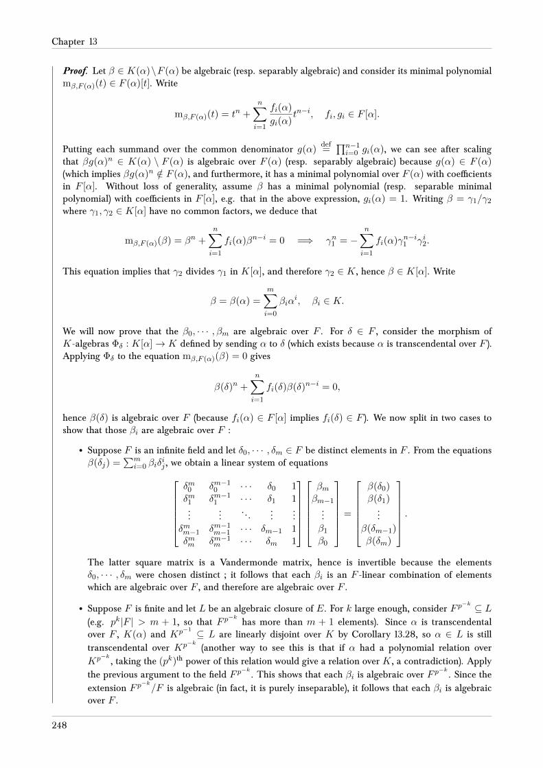
Chapter 13
Proof. Let β ∈ K(α)\F (α) be algebraic (resp. separably algebraic) and consider its minimal polynomialmβ,F (α)(t) ∈ F (α)[t]. Write
mβ,F (α)(t) = tn +n∑i=1
fi(α)
gi(α)tn−i, fi, gi ∈ F [α].
Putting each summand over the common denominator g(α)def=∏n−1i=0 gi(α), we can see after scaling
that βg(α)n ∈ K(α) \ F (α) is algebraic over F (α) (resp. separably algebraic) because g(α) ∈ F (α)(which implies βg(α)n /∈ F (α), and furthermore, it has a minimal polynomial over F (α) with coefficientsin F [α]. Without loss of generality, assume β has a minimal polynomial (resp. separable minimalpolynomial) with coefficients in F [α], e.g. that in the above expression, gi(α) = 1. Writing β = γ1/γ2
where γ1, γ2 ∈ K[α] have no common factors, we deduce that
mβ,F (α)(β) = βn +n∑i=1
fi(α)βn−i = 0 =⇒ γn1 = −n∑i=1
fi(α)γn−i1 γi2.
This equation implies that γ2 divides γ1 in K[α], and therefore γ2 ∈ K , hence β ∈ K[α]. Write
β = β(α) =
m∑i=0
βiαi, βi ∈ K.
We will now prove that the β0, · · · , βm are algebraic over F . For δ ∈ F , consider the morphism ofK-algebras Φδ : K[α]→ K defined by sending α to δ (which exists because α is transcendental over F ).Applying Φδ to the equation mβ,F (α)(β) = 0 gives
β(δ)n +n∑i=1
fi(δ)β(δ)n−i = 0,
hence β(δ) is algebraic over F (because fi(α) ∈ F [α] implies fi(δ) ∈ F ). We now split in two cases toshow that those βi are algebraic over F :
• Suppose F is an infinite field and let δ0, · · · , δm ∈ F be distinct elements in F . From the equationsβ(δj) =
∑mi=0 βiδ
ij , we obtain a linear system of equations
δm0 δm−10 · · · δ0 1
δm1 δm−11 · · · δ1 1
......
. . ....
...δmm−1 δm−1
m−1 · · · δm−1 1δmm δm−1
m · · · δm 1
βmβm−1
...β1
β0
=
β(δ0)β(δ1)
...β(δm−1)β(δm)
.
The latter square matrix is a Vandermonde matrix, hence is invertible because the elementsδ0, · · · , δm were chosen distinct ; it follows that each βi is an F -linear combination of elementswhich are algebraic over F , and therefore are algebraic over F .
• Suppose F is finite and let L be an algebraic closure of E. For k large enough, consider F p−k ⊆ L
(e.g. pk|F | > m + 1, so that F p−k
has more than m + 1 elements). Since α is transcendentalover F , K(α) and Kp−1 ⊆ L are linearly disjoint over K by Corollary 13.28, so α ∈ L is stilltranscendental over Kp−k (another way to see this is that if α had a polynomial relation overKp−k , taking the (pk)th power of this relation would give a relation over K , a contradiction). Applythe previous argument to the field F p
−k. This shows that each βi is algebraic over F p
−k. Since the
extension F p−k/F is algebraic (in fact, it is purely inseparable), it follows that each βi is algebraic
over F .
248

Elementary properties of rings and their modules
Since β /∈ F (α), one of the βi’s does not lie in F . This proves the first part of the claim (i.e thatK \ F contains an element which is algebraic over F , namely that βi not in F ). If we assume ch(F ) =p, β separable over F (α) and the field K does not contain a separable element in K \ F , the field
extension K/F is purely inseparable, so there exists some k ≥ 1 such that βpk
0 , · · · , βpk
m ∈ F (because
β0, · · · , βm ∈ K are algebraic over F ). This means that β(α)pk
=∑m
i=0 βpk
i (αpk)i ∈ F (α), contrary to
the assumption that β was separably algebraic over F (α).
Lemma 13.33. Let E/F be a field extension with structure map ϕ : F → E and S be a set (disjoint fromE). Consider the purely transcendental extension F (S)/F .
(i) The multiplication map E ⊗F F (S)→ E(S) has image the set of polynomial fractions of the form fg
where f ∈ E[S] and g ∈ F [S] \ 0. It follows that the F -algebra E ⊗F F (S) is an integral domainwhose quotient field is isomorphic to E(S) and S is a transcendence basis for the field extensionE(S)/E.
(ii) If E/F is algebraically closed (c.f. Definition 11.38), then E(S)/F (S) is algebraically closed.
(iii) If E/F is separably closed (c.f. Definition 12.7), then E(S)/F (S) is separably closed.
Proof. Consider the following commutative square :
E ⊗F F [S] E ⊗F F (S)
E[S] E(S).
'
The horizontal maps are inclusions and the vertical maps are given by multiplication (i.e. α ⊗ f 7→ αffor α ∈ E and f ∈ F [S]). Since the composition E ⊗F F [S]→ E[S]→ E(S) is injective, inverting theelements of F [S]× gives us an injective map E ⊗F F (S) → E(S) (the map on the right of this square).By construction, its image is the set of fractions where the numerator is in E[S] and the denominatoris in F [S]×. Because E(S) is an integral domain, so does E ⊗F F (S), and the fact that the set ofnumerators contains E[S] implies that the field of fractions of E ⊗F F (S), computed inside E(S), isisomorphic to E(S). We note that the monomials in elements of S form an F -basis of F [S] (because Sis algebraically independent over F ), and tensoring with E over F show that they form an E-basis ofE[S] ; therefore, they are algebraically independent over E as well, i.e. E(S)/E is purely transcendentalwith transcendence basis S. This proves part (i).
To prove part (ii) (resp. part (iii)), we use Lemma 13.32, which gives the case where S is a singleton.Suppose α ∈ E(S) is algebraic (resp. separably algebraic) over F (S). By definition, there exists T ⊆ Ssuch that α ∈ E(T ) is algebraic over F (T ), hence we might as well assume that S is finite. WriteS = s1, · · · , sn. By considering the following diagram of field extensions :
E E(s1) · · · E(s1, · · · , sn−1) E(S)
F F (s1) · · · F (s1, · · · , sn−1) F (S),
the result follows by induction on n.
Lemma 13.34. Let F be a field and K,E be two F -subfields of an algebraically closed field L. Supposethat one of the following conditions hold :
(i) K/F is purely inseparable
249

Chapter 13
(ii) K/F is separably algebraic and E/F is separably closed
(iii) K/F is algebraic and E/F is separably closed
In case (ii), K ⊗F E is a field. In all three cases, K ⊗F E = (K ⊗F E)× ∪ Nil(K ⊗F E), i.e. elements ofK ⊗F E are either units or nilpotents. This implies that (K ⊗F E)red is a field.
Proof. (i) If ch(F ) = 0, we have K = F , hence K ⊗F E ' E is a field. Assume ch(F ) = p > 0 andfix z =
∑ni=1 αi ⊗ βi ∈ K ⊗F E where αi ∈ K and βi ∈ E. Since K/F is purely inseparable,
there exists k ≥ 1 such that for all 1 ≤ i ≤ n, αpk
i ∈ F . It follows that
zpk
=n∑i=1
αpk
i ⊗ βpk
i = 1⊗
(n∑i=1
αpk
i βpk
i
).
lies in the image of E under the map E → K ⊗F E given by β 7→ 1 ⊗ β, which is injective.Therefore, either zp
k= 0 or zp
kis a unit with inverse equal to
zpk−1
1⊗
(n∑i=1
αpk
i βpk
i
)−1 .
(ii) It suffices to show that K ⊗F E is a field. Let z =∑n
i=1 αi ⊗ βi ∈ K ⊗F E where αi ∈ K andβi ∈ E. The F -subfield F (α1, · · · , αn) ⊆ K is separably algebraic, so without loss of generality,assume K/F is finite. By the Primitive Element Theorem, there exists a primitive element λ ∈ Kover F , so that K = F (λ) ' F [t]/(mα,F (t))F [t]. Since K/F is separable, λ is separable overF , hence mα,F (t) ∈ F [t] is an irreducible separable polynomial. By exactness of the functor(−)⊗F E, we have K⊗F E ' E[t]/(mα,F (t))E[t]. The roots of mα,F (t) in L are separable over F ,so since E/F is separably closed, sums of products of roots of mα,F (t) in L are still separable overF , hence either belong to F ∪ (L \ E). It follows that mα,F (t) admits no non-trivial factorizationin E[t], which means it is irreducible over E. This means that E[t]/(mα,(t))E[t] ' K⊗FE is a field.
(iii) The separable closure of F in K , namely Ksep,F , is such that K/Ksep,F is purely inseparable andKsep,F /F is separably algebraic. Since
K ⊗F E ' K ⊗Ksep,F(Ksep,F ⊗F E),
part (ii) implies that Ksep,F ⊗F E is a field, and part (i) implies that any element of K ⊗Ksep,F
(Ksep,F ⊗F E) is either a unit or nilpotent.The conclusion about (K⊗F E)red is clear since if x ∈ (K⊗F E)red\0, we can find a unit x ∈ K⊗F Ewhich maps to x under the projection K ⊗F E → (K ⊗F E)red, which means that x is a unit.
Corollary 13.35. Let E/F be a field extension. For any n ≥ 1, elements of the rings F p−n ⊗F E or
F p−∞ ⊗F E are either units or nilpotents.
Proof. This follows from the fact that the extensions F p−n/F and F p
−∞/F are purely inseparable,
together with Lemma 13.34 (i).
Theorem 13.36. Let E/F be a field extension. The following are equivalent :
(i) The extension E/F is separable
250

Elementary properties of rings and their modules
(ii) For any field extension K/F , the ring K ⊗F E is reduced, i.e. has no non-zero nilpotents
(iii) The ring F p−1 ⊗F E is a field (resp. integral domain, reduced ring)
(iv) The ring F p−n ⊗F E is a field (resp. integral domain, reduced ring) for all n ≥ 1
(v) The ring F p−∞ ⊗F E is a field (resp. integral domain, reduced ring).
(vi) There exists an algebraically closed field Ω such that Ω⊗F E is reduced.
In particular, when F is a perfect field (such as when ch(F ) = 0), the F -algebra K⊗F E is always a reducedring since F p
−1 ⊗F E = F ⊗F E ' E is a field.
Proof. Note : by Lemma 13.34, since F p−1, F p
−nand F p
−∞are purely inseparable extensions of F ,
the conditions of their extensions to E being fields, integral domains or reduced rings are equivalentbecause their elements are units or nilpotents.
( (i) ⇒ (ii) ) By Proposition 13.29, we may assume that E/F is separable and finitely generated, henceseparably generated by MacLane’s criterion (c.f. Theorem 13.31). Let S be a separating transcendencebasis for E/F . It follows by Lemma 13.33 that for any field extension K/F ,
K ⊗F E ' K ⊗F (F (S)⊗F (S) E) ' (K ⊗F F (S))⊗F (S) E ⊆ K(S)⊗F (S) E.
Since E/F (S) is separably algebraic, this means that it suffices to deal with the case where E/F isseparably algebraic (so assume without loss of generality that S = ∅). Let T be a transcendence basis forthe field extension K/F , so that K/F (T ) is algebraic and F (T )/F is purely transcendental. We have
K ⊗F E ' K ⊗F (T ) (F (T )⊗F E) ⊆ K ⊗F (T ) E(T ).
It now suffices to show that K ⊗F (T ) E(T ) is reduced. Since E/F is separably algebraic, E(T )/F (T ) isseparably generated (by the elements of E), thus is separable by MacLane’s criterion and therefore sepa-rably algebraic. Since K/F (T ) is algebraic by assumption, K ⊗F (T ) E(T ) is reduced by Theorem 12.25.
( (ii)⇒ (vi) ) Obvious.
( (vi) ⇒ (iii),(iv),(v) ) Trivial since F p−1 ⊆ F p−n ⊆ F p−∞ ⊆ Ω for all n ≥ 1, hence
F p−1 ⊗F E ⊆ F p
−n ⊗F E ⊆ F p−∞ ⊗F E ⊆ Ω⊗F E.
( (iii)⇒ (i) ) The proof of ( (iv)⇒ (v) ) given in Theorem 12.25 also works when E/F is not algebraic andimplies the result claimed here.
13.3 Rationality of vector spaces with respect to a field extension
Definition 13.37. Let E/F be a field extension.
(i) For an F -vector space V , we let V [E] def= E ⊗F V . We call it the extension of V by scalars to E.
(ii) For an E-vector space W , an F -structure on W is an F -vector subspace V ⊆ W such that thecanonical map ΨE/F : V [E] →W given by multiplication (e⊗ v 7→ ev ∈W ) is an isomorphism. Thecanonical map ΨE/F is called the multiplication map of V over E. (Because of the naturality of thecanonical map, we omit to mention W or V .)
251

Chapter 13
(iii) Let W be an E-vector space with F -structure V .
• An element w ∈W is called F -rational if w ∈ V .
• A subspace W ′ ⊆ W is called F -rational if the canonical map ΨE/F : (W ′ ∩ V )[E] → W hasimage equal to W ′.
• An E-linear map f : W1 → W2 is called F -rational if f(V1) ⊆ V2. The set of F -rationalE-linear maps from W1 to W2 is written HomE/F (W1,W2).
(iv) Let V be an F -vector space. The canonical F -structure on V [E] = E⊗F V is given by the image ofV under the canonical F -linear maps V → E ⊗F V (where v 7→ 1⊗ v). In particular, if the structuremap of E/F is ϕ : F → E, the canonical F -structure of E is given by ϕ(F ).
Remark 13.38. • If E/F is a field extension and W is an E-vector space, let B be an E-basis for
W . If Vdef= 〈B〉F denotes the F -linear subspace spanned by V , then by definition, W = 〈B〉E =
E ⊗F 〈B〉F = V [E]. Conversely, if V is an F -structure for W , an F -basis for V is also an E-basis forW . It follows that any E-vector space admits F -structures.
• If E/F is an isomorphism (e.g. when E = F and the structure map ϕ : F → F is the identity), thereis only one F -structure one can put on the E-vector space W , namely W .
• If W = E[x1, · · · , xn], then Vdef= F [x1, · · · , xn] is an F -structure for W .
• The canonical F -structure for E⊕n is F⊕n via the standard basis e1, · · · , en of both F⊕n andE⊕n. That is what an F -structure is ; a choice of basis for W together with its F -linear span, theF -structure V . Two such bases determine the same F -structure if the identity map is an F -rationalE-linear isomorphism, i.e. if the two chosen bases have the same F -linear span in W .
• An E-linear map f : E⊕n → E⊕m is F -rational (when E⊕n and E⊕m are given their canonical F -structures) if and only if when writing down its matrix form over the standard bases, the coefficientsof the corresponding matrix belong to F . (This means that the map is really just an F -linear mapf : F⊕n → F⊕m but we are extending it to E⊕n and E⊕m.)
• The collection of pairs (W,V ) where W is an E-vector space and V is an F -structure on W ,together with F -rational E-linear maps, form a category (for obvious reasons). We denote it byRatVect(E/F ). It comes with two forgetful functors UE : RatVect(E/F ) → Vect(E) to thecategory of E-vector spaces which forgets the F -structure and UF : RatVect(E/F ) → Vect(F )which only remembers the F -structure V but forgets W ; the F -rationality of the morphisms ensuresthat UF (f) : V1 → V2 is a well-defined F -linear map.
Proposition 13.39. Let E/F be a field extension, W , W1 and W2 be two E-vector subspaces with F -structures V , V1 and V2 respectively.
(i) If we give V [E] its canonical F -structure, the multiplication map V [E] →W is an F -rational isomor-phism of E-vector spaces.
(ii) We have a natural isomorphism of F -vector spaces
HomF (V1, V2) ' HomE/F (V[E]
1 , V[E]
2 ) ' HomE/F (W1,W2)
given by using the isomorphisms V [E]1 ' W1 and V
[E]2 ' W2. This means that the F -structure
HomE/F (W1,W2) on HomE(W1,W2) turns the canonical map
HomF (V1, V2)[E] → HomE(W1,W2)
(i.e. the above isomorphism composed with the multiplication map of HomE/F (W1,W2)) into anatural F -rational E-linear isomorphism.
252

Elementary properties of rings and their modules
(iii) The image of the canonical map
V1 ⊗F V2 →W1 ⊗F W2 →W1 ⊗E W2
is an F -structure onW1⊗EW2 (note that the second map is a quotient of F -vector spaces introducingthe necessary E-linear relations) which turns the canonical map
(V1 ⊗F V2)[E] ' V [E]1 ⊗E V [E]
2 →W1 ⊗E W2
into a natural F -rational E-linear isomorphism.
(iv) The functor UF : RatVect(E/F ) → Vect(F ) has a left-adjoint given by the functor E ⊗F (−),i.e. V 7→ V [E] (equipped with its canonical F -structure), so that the following is a natural F -linearisomorphism :
HomF (V,UF (W )) ' HomE/F (V [E],W ).
(v) There is a natural bijection between the F -rational E-linear subspaces of W and the F -linear sub-spaces of V given by W ′ 7→W ′ ∩ V from left to right and by V ′ 7→ 〈V ′〉E from right to left.
Proof. (i) We already know it is an E-linear isomorphism. The F -rationality is clear since the multi-plication map of V over F induces an isomorphism F ⊗F V1 ' V1 ⊆W1.
(ii) It is clear that HomE/F (W1,W2) is an F -vector space by restricting the E-vector space structureof HomE(W1,W2) to F on HomE/F (W1,W2). In one direction, send f ∈ HomF (V1, V2) to
idE ⊗F f ∈ HomE/F (V[E]
1 , V[E]
2 ). In the other direction, using the isomorphisms V Ei ' Wi, an
F -rational map f ∈ HomE/F (V[E]
1 , V[E]
2 ) corresponds to an F -rational map in HomE(W1,W2)which we can restrict to V1, and the restriction has F -linear image sitting inside V2. These twoconstructions are natural and inverse of each other, thus giving the isomorphism.
(iii) For i = 1, 2, if Bi is an F -basis of Vi, it is also an E-basis ofWi. Therefore, B1⊗F B2def= β1⊗β2 ∈
V1 ⊗ V2 is an F -basis of V1 ⊗F V2 and B1 ⊗E B2 = β1 ⊗ β2 ∈ W1 ⊗E W2 is an E-basis ofW1 ⊗E W2. This implies all the claims.
(iv) By the tensor-hom adjunction,
HomE(V [E],W ) ' HomE(E ⊗F V,W ) ' HomF (V,HomE(E,W )) ' HomF (V,W ).
(v) Let W ′ be an F -rational subspace of W , so that if W has F -structure V , W ′ has F -structureW ′ ∩ V . This implies that 〈W ′ ∩ V 〉E = W , which is one direction. In the other direction, we
see that V ′ ≤ V is an F -structure for W ′def= 〈V ′〉E by definition, and since V [E] ' W is an
isomorphism, we see that W ′ ∩ V = V ′ since W ′ ∩ V corresponds in V [E] to those E-linearcombinations of vectors of V ′ whose coefficients are in F , namely vectors in V ′.
Definition 13.40. Let E/F be a field extension and W be an E-vector space with F -structure V . Equip Ewith its canonical F -structure. An element f ∈ HomE/F (W,E) is called an F -rational E-linear form onW .
Corollary 13.41. Let E/F be a field extension and W be an E-vector space with F -structure V .
(i) IfW ′ is another E-vector space with F -structure V ′ and f : W →W ′ is an F -rational E-linear map,then
• ker f is an F -rational subspace of W
253

Chapter 13
• im f is an F -rational subspace of W ′
• when W ′ is an F -rational subspace of W , W/W ′ can be canonically equipped with the F -structureW ′+V/W ′ ' V/(W ′∩V ) = V/V ′ and the projection map π : W → coker f = W/W ′
is F -rational
• the morphism f is injective (resp. surjective, bijective, zero) if and only if UF (f) : V1 → V2 isinjective (resp. surjective, bijective, zero)
• if W ′′ ⊆ W ′ is an F -rational E-linear subspace, then f−1(W ′′) is an F -rational E-linearsubspace of W
• if W and W ′ are finite-dimensional, then the rank of the E-linear map f is equal to the rank ofthe F -linear map f |V
• if W = W ′ and V = V ′, then f is a nilpotent endomorphism if and only if UF (f) is nilpotent.
(ii) The sum (resp. direct sum) of F -rational E-linear subspaces of W is F -rational.
(iii) The intersection of F -rational E-linear subspaces of W is F -rational.
(iv) An E-linear subspaceW ′ ⊆W is F -rational if and only if there exists a family of F -rational E-linearforms Φ ⊆ HomE/F (W,E) such that W ′ =
⋂f∈Φ ker f .
Proof. (i) Consider the following commutative diagram with exact rows and columns :
0 0 0 0
0 ker f W W ′ coker f 0
0 (ker f |V )[E] V [E] (V ′)[E] coker f |[E]V 0
0 0 0 0
f
ιker f
f
ιV ιV ′ ιcoker f
where the maps denoted by ι are the multiplication maps.
• Suppose that f is surjective (onto im f for instance). An application of Snake’s lemma showsthat ker f ' (ker f |V )[E] and im f ' (im f |V )[E].
• Suppose that f is injective (after modding out the F -rational subspace ker f for instance).Another application of Snake’s lemma shows that coker f ' (coker f |V )[E].
• If W ′ is an F -rational subspace of W , the latter point means that V/V ′ is an F -structure onW/W ′ such that the projection W →W/W ′ is F -rational.
• The latter arguments imply that ker f (resp. im f, coker f ) is equal to zero if and only ifker f |V (resp. im f, coker f |V ) is equal to zero.
• The E-linear subspace f−1(W ′′) is the kernel of the composition of the F -rational maps
Wf→W ′ →W ′/W ′′, hence is F -rational.
• From im f = (im f |V )[E], we deduce the equality on the ranks of f and f |V .• From im (fn) = (im (f |V )n)[E], it is clear that for any n ≥ 1, we have fn = 0 if and only if
(f |V )n = 0.
(ii) Let Wii∈I be a family of F -rational vector spaces where Wi has F -structure Vi. Then⊕
i∈IWi
has F -structure equal to⊕
i∈I Vi. If the Wi are assumed to be F -rational E-linear subspaces of avector space W with F -structure V , their sum is the image of the F -rational map
⊕i∈IWi → W
given by summing the inclusion maps, thus is F -rational by part (i).
254

Elementary properties of rings and their modules
(iii) Let Wii∈I be a family of F -rational E-linear subspaces of an E-vector space E. Their inter-section is the kernel of the direct sum of the projections W → W/Wi (which are F -rational bypart (i)), i.e. the kernel of W →
⊕i∈IW/Wi. This kernel is rational by part (i) again.
(iv) (⇒) Fix an F -basis B′ of W ′ ∩ V and extend it to an F -basis B of V . For each β ∈ B, considerthe F -rational form fβ mapping a vector w ∈ W to its coefficient in front of β under itsdecomposition over the basis. In other words, fβ(
∑γ∈B eγγ) = eβ where eγ ∈ E. It follows that
W ′ =⋂β∈B\B′ ker fβ .
(⇐) The F -rational forms fβ are F -rational by definition, so their kernels (and the intersection ofthose kernels) is F -rational.
To study rationality via automorphisms of E/F , we will need the automorphism group to behave wellwith respect to the extension. To this purpose, we define the notion of perfectly normal extensions (c.f.Definition 13.43).
Lemma 13.42. Let E/F be an algebraic extension and Ω be an algebraic closure for E, so that F p−∞ ⊆ Ω
is defined. Then E/F is normal if and only if EAut(E/F ) ⊆ F p−∞
. (In characteristic zero, interpret this asEAut(E/F ) = F .)
Proof. Consider the separable closure of F in E, denoted by Esep,F ⊆ E and equal to theset of all elements of E separable over F . Note that restriction to Esep,F is a map of groupsAut(E/F ) → Aut(Esep,F /F ) which is an isomorphism because the extension E/Esep,F is purelyinseparable, hence an F -automorphism of Esep,F admits a unique lift to E. The fact that the restrictionis well-defined follows from the fact that automorphisms in Aut(E/F ) permutes roots of separablepolynomials over F .
(⇒) Since E/F is normal, any irreducible polynomial in F [t] with a root in Esep,F is separable andsplits in E, hence splits in Esep,F ; this means Esep,F /F is separable, hence Galois. It follows that
EAut(Esep,F /F )sep,F = F . Let α ∈ EAut(E/F ). Then αp
n ∈ Esep,F for some n ≥ 1 and αpnis still fixed
by each automorphism of Aut(E/F ), hence αpn ∈ F , which means α ∈ F p
−n. We deduce that
EAut(E/F ) ⊆ F p−∞ .
(⇐) Let F ′def= E∩F p−∞ ⊆ E. Since σ ∈ Aut(E/F ) clearly fixes F ′, we have Aut(E/F ) = Aut(E/F ′).
It follows that EAut(E/F ′) ⊆ (F ′)p−∞
= F ′, hence we obtain equality. If E′ ⊆ E is an arbitrary finiteF ′-subfield, let E′ ⊆ E′′ ⊆ E be the F ′-subfield of E which is closed under the action of Aut(E/F ′) ; itis still finite over F ′ (take generators for E′/F ′ and see that the orbits of those generators in E generateE′′). It follows that (E′′)Aut(E′′/F ′) ⊆ EAut(E/F ′) = F ′, hence we get equality. This means E′′/F ′ hasenough automorphisms, hence is normal. Given any irreducible polynomial with coefficients in F ′ and
a root α ∈ E, applying the previous result to E′def= F (α) ⊆ E shows that E contains a finite normal
extension E′′ containing F (α), hence the minimal polynomial of α (our original irreducible polynomial)splits over E′′, hence over E. This means E/F ′ is normal.
If f(t) ∈ F [t] is an irreducible polynomial with a root in E, since F [t] ⊆ F ′[t], f(t) splits over E, henceE/F is also normal.
Definition 13.43. Let E/F be a field extension. We say that this extension is called
(i) normal if EAut(E/F ) ⊆ F p−∞
255

Chapter 13
(ii) perfectly normal if EAut(E/F ) = F
(iii) a generalized Galois extension if it is normal and separable.
Remark 13.44. Let E/F be a field extension.
• Perfectly normal field extensions are normal since F ⊆ F p−∞ .
• Normality and perfect normality are the same property when E/F is separable since E and F p−∞
are linearly disjoint over F . In particular, they are the same property when F is perfect, e.g. incharacteristic zero. It follows that generalized Galois extensions are perfectly normal.
• By the preceding point, any Galois extension (not generalized Galois, i.e. algebraic Galosi extensions)is perfectly normal.
• If E is algebraically closed, then E/F is perfectly normal ; this follows from Theorem 13.16.
• Purely transcendental extensions are perfectly normal. This is obvious since an F -automorphismF (S) → F (S)× corresponds to a map of sets S → F (S) \ F , so if α ∈ F (S) \ F , we can choose amap σ : S → F (S) \ F where s ∈ S \ α maps to α, hence σ−1 ∈ Aut(F (S)/F ) maps α to s ; thisconcludes the argument unless S = s and α = s, in which case we can many automorphisms ofF (s) which do not fix s (any map of sets s → F (S) \ F will do).
Proposition 13.45. Let E/K and K/F be normal (resp. perfectly normal, generalized Galois) extensions.Then E/F is normal (resp. perfectly normal, generalized Galois).
Proof. We first deal with the perfectly normal case. We have EAut(E/F ) ⊆ EAut(E/K) = K , henceEAut(E/F ) ⊆ KAut(K/F ) = F . In the normal case, write ch(F ) = p > 0 and pick α ∈ EAut(E/F ). SinceEAut(E/K) ⊆ Kp−∞ , there exists n ≥ 1 such that αp
n ∈ K . It follows that αpn ∈ KAut(K/F ) ⊆ F p
−∞,
hence EAut(E/F ) ⊆ F p−∞
. The case where the extensions are generalized Galois extensions follows byProposition 13.29 (ii).
Corollary 13.46. Let E/F be a field extension with transcendence basis S (resp. separating transcendencebasis) such that E/F (S) is normal (resp. Galois). Then E/F is perfectly normal (resp. normal). Inparticular, if E is algebraically closed, then E/F is perfectly normal.
Proof. We already know that F (S)/F is perfectly normal by Remark 13.44, so if E/F (S) is normal,so does E/F by Proposition 13.45. If S is a separating transcendence basis, E/F (S) is normal andseparable, thus perfectly normal by Remark 13.44.
Definition 13.47. Let E/F be a field extension, W be an E-vector space and V an F -structure on W . Forσ ∈ Aut(E/F ), we let
gσdef= ΨE/F (σ ⊗F idV ) Ψ−1
E/F ∈ AutF (W )
or in other words, it is the unique map completing the following commutative square
V [E] V [E]
W W.
σ⊗idV
ΨE/F ΨE/F
gσ
The commutative square shows that gσ1 gσ2 = gσ1σ2 . For β =∑n
i=1 αivi where vi ∈ V and αi ∈ E, wehave gσ(β) =
∑ni=1 σ(αi)vi.
256
Elementary properties of rings and their modules
Remark 13.48. The map σ 7→ gσ induces an F -linear action of Aut(E/F ) on W . If Kdef= EAut(E/F ), the
set of fixed points of this action is precisely the image of the multiplication map ΨK/F : V [K] →W . WhenE/F is perfectly normal, the set of fixed points is equal to V .
Proposition 13.49. Let E/F be a perfectly normal extension, W ,W1,W2 be three E-vector spaces withrespective F -structures V ,V1,V2.
(i) An element w ∈W is F -rational if and only if gσ(w) = w for all σ ∈ Aut(E/F ).
(ii) An E-linear subspace W ′ ⊆ W is F -rational if and only if gσ(W ′) ⊆ W ′ for all σ ∈ Aut(E/F ),which implies gσ(W ′) = W ′.
(iii) If f : W1 → W2 is an E-linear map, it is F -rational if and only if it commutes with gσ for allσ ∈ Aut(E/F ), i.e. f gW1
σ = gW2σ f .
Proof. (i) Under the isomorphism ΨE/F : V [E] →W , the element w ∈W corresponds to a finite sum∑ni=1 αi ⊗ vi where α1, · · · , αn ∈ E and v1, · · · , vn ∈ V and the automorphism gσ corresponds
to σ ⊗ idV . The element w ∈ W is F -rational if and only if α1, · · · , αn ∈ F = EAut(E/F ), i.e. ifand only if σ(αi) = αi for all σ ∈ Aut(E/F ) and i = 1, · · · , n.
(ii) If W ′ is F -rational, let V ′def= W ′ ∩ V . Pick an F -basis of V ′ and extend it to an F -basis B of
V . For every w ∈ W ′, write w =∑n
i=1 αivi where α1, · · · , αn ∈ F . It follows that gσ(w) = w,hence gσ(W ′) ⊆ W ′. Conversely, if we let B be an F -basis for V and writing w ∈ W ′ as before,gσ(w) = w for all σ ∈ Aut(E/F ) implies that α1, · · · , αn ∈ EAut(E/F ) = F , hence w ∈W ′ ∩ V .
(iii) Suppose f is F -rational and let w ∈ W . Write w =∑n
i=1 αivi where v1, · · · , vn ∈ V1 andα1, · · · , αn ∈ E. The F -rationality of f implies
gW2σ (f(w)) =
n∑i=1
σ(αi)f(vi) = f(gW1σ (w)).
Conversely, suppose f commutes with the action given by gσ and let w ∈ W . We wish to showthat f(V1) ⊆ V2, so pick v ∈ V1 and write f(v) =
∑ni=1 αivi for some v1, · · · , vn ∈ V2 linearly
independent over F , hence also over E. We have
n∑i=1
αivi = f(v) = f(gW1σ (v)) = gW2
σ (f(v)) =
n∑i=1
σ(αi)gσ(vi) =
n∑i=1
σ(αi)vi
which implies αi = σ(αi) for all σ ∈ Aut(E/F ), hence αi ∈ F and f is F -rational.
Corollary 13.50. Let E/F be a perfectly normal field extension and V an F -vector space. Let Aut(E/F )
act on V [E] = E ⊗F V by letting σ · (α ⊗ v)def= σ(α) ⊗ v. If W ′ ≤ V [E] is stable under the action of
Aut(E/F ), then there exists a unique F -vector subspace V ′ ≤ V such that W ′ = E ⊗F V ′.
Proof. By equipping V [E] with its canonical F -structure, the stability of W ′ under the action ofAut(E/F ) tells us that W ′ is F -rational by Proposition 13.49 (ii), hence that there exists V ′ ≤ Vsuch that W ′ = 〈V ′〉E = E ⊗F V ′.
Lemma 13.51. Let F be a field and V a finite-dimensional F -vector space. Given a subset H ⊆ V ∗def=
HomF (V, F ) such that⋂h∈H kerh = 0, then 〈H〉F = V ∗.
257

Chapter 13
Proof. We re-phrase this in the following way. Recall that finite-dimensional F -vector spaces can beidentified with their double duals. Let W be a finite-dimensional F -vector space and interpret w ∈ Was a linear form on W ∗ via the natural isomorphism W 'W ∗∗. Suppose H ⊆W is such that⋂
w∈Hkerw = ψ ∈ HomF (W,F ) | ψ(H) = 0 = 0.
Consider the linear subspace 〈H〉F ≤ W . If it is a proper subspace, extending a basis of 〈H〉F to abasis of W proves the existence of a non-zero linear form on W which vanishes on H , a contradiction.Therefore 〈H〉F = W . We now apply this result to W = V ∗ and deduce the lemma.
Theorem 13.52. Let Ω/E and E/F be two field extensions where Ω is an algebraically closed field. Thefollowing are equivalent :
(i) For any finite-dimensional F -vector subspace V of E, an F -linear map ψ : V → Ω is an Ω-linearcombination of restrictions of automorphisms σ1, · · · , σn ∈ Aut(Ω/F ) to V .
(ii) For any α1, · · · , αn ∈ E, there exists σ1, · · · , σn ∈ Aut(Ω/F ) such that the matrix (σi(αj)) ∈Matn×n(Ω) is invertible
(iii) If X denotes the set of morphisms of Ω-algebras φ : Ω⊗F E → Ω, the following equality holds :⋂φ∈X
kerψ = 0.
(iv) The extension E/F is separable.
Proof. ( (i) ⇒ (ii) ) Let Vdef= 〈α1, · · · , αn〉F ⊆ E be the F -linear span of our F -linearly independent
elements α1, · · · , αn. The map
Φ : HomF (V,Ω)→ Ωn, (ψ : V → Ω) 7→ (ψ(α1), · · · , ψ(αn))
is an isomorphism (this is elementary linear algebra since it’s the isomorphism HomF (F,Ω) ' Ω forn = 1). The F -linear maps σ|V | σ ∈ Aut(Ω/F ) span HomF (V,Ω) as a Ω-=vector space byassumption, so choose σ1, · · · , σn such that σ1|V , · · · , σn|V forms an Ω-basis of HomF (V,Ω). BecauseΦ is an isomorphism, it follows that the vectors
(σ1(α1), · · · , σ1(αn)), · · · , (σn(α1), · · · , σn(αn))
form a basis of Ωn. Considering the matrix (σi(αj))ij ∈ Matn×n(Ω), the above says that this matrix haslinearly independent rows, hence is invertible.
( (ii) ⇒ (iii) ) Letβ ∈
⋂ψ∈HomΩ(Ω⊗FE,Ω)
kerψ ⊆ Ω⊗F E
and write β =∑n
j=1 γj ⊗ αj . We want to show that β = 0. Without loss of generality, we can assumethat the set α1, · · · , αn is linearly independent over F . Choose σ1, · · · , σn ∈ Aut(Ω/F ) such that the
matrix (σi(αj)) ∈ Matn×n(Ω) is invertible. Set ψidef= idΩ ⊗ σi : Ω⊗K L→ Ω, i.e. ψi(x⊗ e) = xσi(e).
The maps ψ1, · · · , ψn are Ω-linear by construction, so
∀i = 1, · · · , n,n∑j=1
γj σi(αj) = ψi(β) = 0.
258

Elementary properties of rings and their modules
We deduce that σ1(α1) · · · σ1(αn)...
. . ....
σn(α1) · · · σn(αn)
γ1
...γn
= 0 =⇒ γ1 = · · · = γn = 0.
( (iii) ⇒ (iv) ) We may assume ch(F ) = p since any field extension of characteristic zero is separable.We show that the F -algebra Ω ⊗F E is reduced (c.f. Theorem 13.36). Define Φ : Ω ⊗F E → ΩX by
Φ(z)def= (φ(z))φ∈X . We have ker Φ =
⋂φ∈X kerφ = 0, so Φ is injective ; this means that Ω ⊗F E can
be seen as an Ω-subalgebra of the Ω-algebra ΩX , which is reduced. Therefore Ω⊗F E is reduced.
( (iv) ⇒ (i) ) Let V be an F -vector subspace of E and set V [Ω] def= Ω ⊗F V . Let Ψ : V [Ω] → 〈V 〉Ω ⊆ Ω
denote the Ω-linear form given by
∀α ∈ Ω, v ∈ V, Ψ(α⊗ v)def= αv ∈ ΩV ⊆ ΩL = Ω.
(This is not the map ΨΩ/F from Section 13.3 since 〈V 〉Ω does not have dimension dimF V as an Ω-vectorspace, but 1. The reason is because V is not an F -structure for 〈V 〉Ω.)
For σ ∈ Aut(Ω/F ), let σVdef= σ ⊗ idV : V [Ω] → V [Ω] and hσ
def= σ Ψ σ−1
V : V [Ω] → Ω (note thatσ−1V = (σ−1)V and that this hσ is not equal to gσ = ΨΩ/F σV Ψ−1
Ω/F as in Section 13.3). To illustrate,we have the following commutative diagrams (W is some Ω-vector space with F -structure V ) :
V [Ω] V [Ω]
Ω Ω,
σV
Ψ hσ
σ
V [Ω] V [Ω]
W W
ΨΩ/F
σV
ΨΩ/F
gσ
The map hσ is Ω-linear since
hσ(α⊗ v) = σ(Ψ(σ−1(α)⊗ v)) = σ(σ−1(α)v) = ασ(v) = αhσ(1⊗ v).
We deduce that kerhσ is an Ω-linear subspace of V [Ω], and so does W ′def=⋂σ∈Aut(Ω/F ) kerhσ . For
σ, σ′ ∈ Aut(Ω/F ),hσ = σ hidΩ
σ−1V =⇒ σ hσ′ σ−1
V = hσσ′ ,
hence we see that σV (W ′) ⊆ W ′ for all σ ∈ Aut(Ω/F ). We give V [Ω] the F p−∞
-structure
V [F p−∞
] ⊆ V [Ω] ; since Aut(Ω/F ) = Aut(Ω/F p−∞
) and Ω/F p−∞
is perfectly normal by Corol-
lary 13.46, there exists a unique (F p−∞
)-vector subspace V ′ ≤ V [F p−∞
] such that W ′ = (V ′)[Ω] byCorollary 13.50. By definition of separability, E and F p
−∞are linearly disjoint over F , which means V
and F p−∞
are linearly disjoint over F . It follows that the multiplication map F p−∞⊗F L→ F p
−∞L ⊆ Ω
is injective, and therefore also injective when restricted to F p−∞ ⊗F V = V [F p
−∞] ; note that this is the
restriction of Ψ to V [F p−∞
]. If we restrict even further to V ′, we see that it becomes Ψ|V ′ = hidΩ|V ′ = 0,
hence V ′ = 0, which means W ′ = 〈V ′〉Ω = 0.
By Lemma 13.51, this implies that hσ ∈ HomΩ(V [Ω],Ω) | σ ∈ Aut(Ω/F ) spans HomΩ(V [Ω],Ω). Underthe tensor-hom adjunction
HomΩ(V [Ω],Ω) ' HomΩ(V ⊗F Ω,Ω) ' HomF (V,HomΩ(Ω,Ω)) ' HomF (V,Ω),
the element hσ ∈ HomΩ(V [Ω],Ω) corresponds to σ|V : V → Ω. This means that the F -automorphismsof Ω restricted to V , namely the σ|V for σ ∈ Aut(Ω/F ), span HomF (V,Ω) as an Ω-vector space, whichcompletes the proof.
259

Chapter 13
13.4 Norms, Traces and Determinants
Definition 13.53. Let E/F be a finite field extension. Given α ∈ E, one can consider the map Lα : E → Egiven by multiplication by α, i.e. β ∈ E maps to αβ. This map is E-linear, and in particular F -linear, soif we fix an F -basis α1, · · · , αn of E, we can write Lα(αj) =
∑ni=1 aijαi for some aij ∈ F . The matrix
(aij) ∈ Matn×n(F ) is the matrix representation of Lα.
(i) The trace map of E/F is the F -linear map TrE/F (−) : E → F defined by TrE/F (α)def= tr(Lα) =∑n
i=1 aii.
(ii) The norm map of E/F is the map NE/F (−) : E → F defined by NE/F (α)def= det(Lα) =
det((aij)). Note that det(Lα) is always non-zero for α ∈ E× since Lα is an invertible map withinverse Lα−1 , hence we usually see the norm as a map NE/F (−) : E× → F×.
(iii) Given a subset B = α1, · · · , αn ⊆ E, the discriminant of this subset is defined as the determinantof the matrix (TrE/F (αiαj))ij ∈ Matn×n(F ). We denote it by ∆E/F (B).
(iv) Given α ∈ E, the characteristic polynomial of α over F is defined as
χE/Fα (t)def= det(t idE − Lα) = t[E:F ] − TrE/F (α) t[E:F ]−1 + · · ·+ (−1)[E:F ]NE/F (α) ∈ F [t].
Note that we consider the determinant as that of the F [t]-linear endomorphism t idE − Lα ∈EndF [t](E[t]), so that t idE is really t idE[t] (but when we think of those as polynomials in t withendomorphisms as coefficients, it doesn’t really help). It follows that the determinant lies in F [t]. Thelatter equality follows from ?? (this will be added in the future, but I know the proof : contact me ifyou need it).
Proposition 13.54. Let E/F be a finite field extension and α ∈ E.
(i) The minimal polynomial of α over F divides the characteristic polynomial of α over F , i.e. mα,F (t)
divides χE/Fα (t) in F [t].
(ii) If E = F (α), then mα,F (t) = χE/Fα (t).
(iii) If K/F is any field extension in which χE/Fα (t) splits as χE/Fα (t) =∏[E:F ]i=1 (t− αi), then
TrE/F (α) =
[E:F ]∑i=1
αi, NE/F (α) =
[E:F ]∏i=1
αi.
Remark 13.55. Note that χE/Fα (t) obviously depends on both E and F , unlike the minimal polynomial :
for starters, replacing F by an F -subfield of E or E by an F -subfield of F changes the degree of χE/Fα (t),which is equal to [E : F ].
Proof. (i) Substituting Lα for t, we see that χE/Fα (Lα) = det(LαidE − Lα) = det(0) = 0. It follows
that χE/Fα (α)β = 0 for all β ∈ E, and in particular for β = 1, so that χE/Fα (α) = 0. By definitionof the minimal polynomial, this gives the result.
(ii) The polynomial χE/Fα (t) is monic of degree [E : F ] = [F (α) : F ]. Since mα,F (t) also satisfies
those two properties and divides χE/Fα (t) by part (i), we obtain equality.
260

Elementary properties of rings and their modules
(iii) This follows by comparing coefficients in the following equality in K[t] :
t[E:F ] − TrE/F (α) t[E:F ]−1 + · · ·+ (−1)[E:F ]NE/F (α) = χE/Fα (t) =
[E:F ]∏i=1
(t− αi)
= t[E:F ] −
[E:F ]∑i=1
αi
t[E:F ]−1 + · · ·+ (−1)[E:F ]
[E:F ]∏i=1
αi.
Lemma 13.56. Let E/K and K/F be two finite field extensions. For all α ∈ K , we have
χE/Fα (t) =(χK/Fα (t)
)[E:K], NE/F (α) = NK/F (α)[E:K] , TrE/F (α) = [E : K]TrK/F (α) .
Proof. We begin with the first equality. Let A def= α1, · · · , αn be an F -basis of K and Bβ1, · · · , βm
be a K-basis of E. By Theorem 11.34 (and its proof), the set
C def= αiβj | 1 ≤ i ≤ n, 1 ≤ j ≤ m
is an F -basis of E. Letting LKα ∈ EndF (K) and LEα ∈ EndF (E) denote the corresponding multiplicationby α maps in K and E, if we write [LKα ]A and [LEα ]C for the corresponding matrix forms, we can put[LEα ]C in the following block form :
[LEα ]C =
[LKα ]A 0 · · · 0
0. . . . . .
......
. . . . . . 00 · · · 0 [LKα ]A
where the zeros in this block form represent n × n blocks of zeros. Taking characteristic polynomialsproves the first equality. As for the second and third, note that(tn − TrK/F (α) tn−1 + · · ·+ (−1)nNK/F (α)
)m= tnm−nTrK/F (α) tnm−1+· · ·+
((−1)nNK/F (α)
)mimplies the result.
Corollary 13.57. Let E/F be a finite field extension and α ∈ E. Then E = F (α) if and only if mα,F (t) =
χE/Fα (t).
Proof. It follows from the fact that χE/Fα (t) =(χF (α)/Fα (t)
)[E:F (α)]= (mα,F (t))[E:F (α)] by Proposi-
tion 13.54 (ii).
Theorem 13.58. Let E/F be a finite field extension, α ∈ E and L be an algebraic closure for E. Letσi : E → L be one of the [E : F ]sep distinct F -embeddings of E into L for i ranging from 1 to [E : F ]sep.Then
χE/Fα (t) =
[E:F ]sep∏i=1
(t− σi(α))
[E:F ]ins
261

Chapter 13
In particular, as a corollary, we get
TrE/F (α) = [E : F ]ins
[E:F ]sep∑i=1
σi(α)
, NE/F (α) =
[E:F ]sep∏i=1
σi(α)
[E:F ]ins
.
Proof. In the case where E = F (α), χE/Fα (t) = mα,F (t), and the σi(α) are simply the distinct roots ofmα,F (t). There are deg mα,F,sep = [E : F ]sep such roots and they appear with multiplicity deg mα,F,ins =[E : F ]ins, so the formula holds. In general, since [E : F ]sep = [E : F (α)]sep[F (α) : F ]sep and there are
[E : F (α)]sep =[E : F
(α[F (α):F ]ins
)]sep
[F(α[F (α):F ]ins
): F (α)
]sep
=[E : F
(α[F (α):F ]ins
)]sep
many F -embeddings of E which fix the element σi(α) (because they restrict to the identity on F (σi(α)))together with the fact that there are[
F(α[F (α):F ]ins
): F]
sep=
[F (α) : F ]sep[F (α) : F
(α[F (α):F ]ins
)]sep
= [F (α) : F ]sep
many distinct roots of the minimal polynomial of α[F (α):F ]ins (or equivalently, of the minimal polynomialof α, whose ([F (α) : F ]ins)
th powers are the roots of the minimal polynomial of α[F (α):F ]ins ), we deducethat [E:F ]sep∏
i=1
(t− σi(α))
[F (α):F ]ins
=
[E:F ]sep∏i=1
(t[F (α):F ]ins − σi
(α[F (α):F ]ins
))= mα[F (α):F ]ins ,F
(t[F (α):F ]ins
)[E:F (α)]sep
= mα,F,sep
(t[F (α):F ]ins
)[E:F (α)]sep
= mα,F (t)[E:F (α)]sep .
Raising both sides to the ([E : F (α)]ins)th power completes the proof since by Corollary 13.57,
(mα,F (t))[E:F (α)] =(χF (α)/Fα (t)
)[E:F (α)]= χE/Fα (t).
Comparing the coefficients in front of t0 and t[E:F ]−1 gives the two equalities as a corollary.
Corollary 13.59. Let E/F be a finite separable extension and α ∈ E. Fix an algebraic closure L for E.Write Emb(E/F ) = σ1, · · · , σ[E:F ] for the set of F -embeddings σi : E → L. Then
χE/Fα (t) =
[E:F ]∏i=1
(t− σi(α)), TrE/F (α) =
[E:F ]∑i=1
σi(α), NE/F (α) =
[E:F ]∏i=1
σi(α).
Proof. Straightforward from Theorem 13.58 since [E : F ]ins = 1.
Proposition 13.60. Let E/K and K/F be finite field extensions.
(i) The map TrE/F (−) : E → F is F -linear and the map NE/F (−) : E× → F× is a morphism ofgroups.
(ii) For all α ∈ F and β ∈ E, we have NE/F (αβ) = α[E:F ]NE/F (β).
262

Elementary properties of rings and their modules
(iii) For all α ∈ E, we have
TrE/F (α) = TrK/F(TrE/K (α)
), NE/F (α) = NK/F
(NE/K (α)
),
Proof. Part (i) follows from the linearity of the trace and the multiplicativity of the determinant onendomorphisms of an F -vector space. Since α ∈ F , there is only one F -embedding of F into analgebraic closure of E, so Corollary 13.59 gives NE/F (α) = αn. Part (ii) then follows from part (i).
Let L/E be a normal closure for L/F . Consider the subgroups Aut(L/E) ≤ Aut(L/K) ≤Aut(L/F ). If we choose representatives ϕi ∈ Aut(L/K) and ψj ∈ Aut(L/F ) for the coset spacesAut(L/F )/Aut(L/K) and Aut(L/F )/Aut(L/E) respectively, we obtain partitions
Aut(L/K) =
[E:K]sep⋃i=1
ϕi Aut(L/E), Aut(L/F ) =
[K:F ]sep⋃j=1
ψj Aut(L/K)
The set of coset representatives correspond to extensions of an embedding ϕ : K → L to an embeddingϕ′ : E → L (resp. ψ : F → L to ψ′ : K → L) because two automorphisms of L which restrict to thesame embedding of E into L represent the same coset of Aut(L/K)/Aut(L/E) (do the same reasoningwith Aut(L/F )/Aut(L/K)). Combining the two equalities, we obtain
Aut(L/F ) =
[E:K]sep⋃i=1
[K:F ]sep⋃j=1
ψjϕi Aut(L/E).
Note that this means that ϕ1|E , · · · , ϕ[E:F ]sep|E : E → L are the distinct K-embeddings of E into L,
ψ1|K , · · · , ψ[K:F ]sep|K : K → L are the distinct F -embeddings of K into L and then ψjϕi|K : K → L
are the distinct F -embeddings of K into L. By Theorem 13.58, this implies
TrE/F (α) = [E : F ]ins
[K:F ]sep∑j=1
[E:K]sep∑i=1
ψj(ϕi(α))
= [K : F ]ins
[K:F ]sep∑j=1
ψj
[E : K]ins
[K:F ]sep∑i=1
ϕi(α)
= [K : F ]ins
[K:F ]sep∑j=1
ψj(TrE/K (α)
)= TrK/F
(TrE/K (α)
).
The same argument gives NE/F (α) = NK/F
(NE/K (α)
); just replace addition by multiplication (and
the [E : F ]ins, [E : K]ins and [K : F ]ins factors by exponents).
Theorem 13.61. Let E/F be a finite field extension. The following are equivalent :
(i) The F -bilinear form TrE/F (−,−) : E × E → F defined by TrE/F (α, β)def= TrE/F (αβ) is non-
degenerate
(ii) There exists α ∈ E satisfying TrE/F (α) 6= 0
(iii) The map TrE/F (−) : E → F is surjective
(iv) The extension E/F is separable.
263

Chapter 13
Proof. We may assume ch(F ) = p.
( (ii) ⇐⇒ (iii) ) This is clear since TrE/F (−) is an F -linear map.
( (i) ⇒ (ii) ) If TrE/F (−,−) is non-degenerate, this means that the map (α 7→ TrE/F (−, α)) :E → HomF (E,F ) is an isomorphism. Picking a direct sum decomposition of F -vector spacesE = F ⊕M and letting πF : E → F denote the corresponding projection, there exists α ∈ E such thatTrE/F (α) = TrE/F (1, α) = πF (1) = 1 6= 0.
( (iii) ⇒ (iv) ) The extension E/F is separable if and only if [E : F ]ins = 1, but Theorem 13.58 impliesthat if [E : F ]ins > 1, it is a power of p greater than 1, hence TrE/F (−) = 0. So if TrE/F (−) 6= 0,[E : F ]ins = 1.
( (iv) ⇒ (i) ) Set ndef= [E : F ]. Since E/F is finite and separable, we can find α ∈ E such that
E = F (α) by the Primitive Element Theorem. This means 1, α, · · · , αn−1 is an F -basis for E.
Over this basis, the matrix form of TrE/F (−,−) has the form Adef= (aij) ∈ Matn×n(F ) where
aij = TrE/F(αi−1αj−1
)= TrE/F
(αi+j−2
), so it suffices to show that detA 6= 0.
Let L be a splitting field for mα,F (t) over E. Because E/F is separable, mα,F (t) has n distinct roots inL, say α1, · · · , αn. It follows that
TrE/F (α) =n∑i=1
αi.
Since E = F (α), we also have mα,F (t) = χE/Fα (t), so the fact that the latter polynomial has distinct
roots implies that the multiplication by α map Lα : E → E is diagonalizable over L (i.e. the linear mapL⊗F Lα : L⊗F E → L⊗F E is an L-linear diagonalizable map with eigenvalues equal to α1, · · · , αn).We deduce that Lkα = Lαk is diagonalizable too with eigenvalues equal to αk1 , · · · , αkn for any integerk ≥ 1, which means
TrE/F
(αk)
=n∑i=1
αki .
Consider the Vandermonde matrix V = (vij) where vij = αj−1i . The product V V > has (i, j)th coefficient
equal to
n∑k=1
vikv>kj =
n∑k=1
vikvjk =n∑k=1
αi−1k αj−1
k =n∑k=1
αi+j−2k = TrE/F
(αi+j−2
)= aij ,
which means V V > = A. We deduce that detA = detV 2 6= 0 because the Vandermonde matrix hasdeterminant equal to
detV =∏
0≤i<j≤n−1
(αj − αi) 6= 0.
Corollary 13.62. Let E/F be a finite field extension with F -basis B def= α1, · · · , αn. Then E/F is
separable if and only if ∆E/F (B) 6= 0. In particular, when E/F is separable, for any basis B, we have∆E/F (B) 6= 0.
Proof. We know that E/F is separable if and only if the bilinear form TrE/F (−,−) is non-degenerate.Over the basis B, the matrix form of TrE/F (−,−) is precisely (TrE/F (αi, αj))ij , whence
det((TrE/F (αi, αj))ij) = ∆E/F (α1, · · · , αn) = ∆E/F (B) .
264

Elementary properties of rings and their modules
Therefore E/F is separable if and only if ∆E/F (B) is nonzero for some B, in which case it is non-zerofor all B.
Proposition 13.63. Let E/F be a finite field extension with F -basis B = α1, · · · , αn. Suppose C =γ1, · · · , γn ⊆ E is another subset and write
γj =
n∑i=1
cijαi, cij ∈ F.
Then ∆E/F (C) = det(cij)2∆E/F (B). In particular, when E/F is separable, C is an F -basis for E if and
only if ∆E/F (C) 6= 0.
Proof. Let C = (cij) and let ϕ : E → E be the corresponding F -linear endomorphism of E whose
expression over the basis B is equal to C . Let Adef= (TrE/F (αiαj))ij . It follows that
det((TrE/F (γi, γj))ij) = det((TrE/F (ϕ(αi), ϕ(αj)))ij) = det(C>AC) = det(C)2∆E/F (B) .
Clearly C is a F -basis if and only if detC 6= 0, which gives the result.
Proposition 13.64. Let E/F be a finite separable extension of degree n and write Emb(E/F ) = σ1, · · · , σnfor the distinct F -embeddings of E into a normal closure for E/F . If A = α1, · · · , αn ⊆ E is any subsetof n elements, then
∆E/F (A) = det((σi(αj))ij)2.
Proof. This is just a computation :
∆E/F (A) = det((TrE/F (αi, αj))ij)
= det
( n∑k=1
σk(αiαj)
)ij
= det
( n∑k=1
σk(αi)σk(αj)
)ij
= det
((σi(αj))
>ij(σi(αj))ij
)= det((σi(αj))ij)
2.
Definition 13.65. Let E/F be a finite field extension of degree n. For α ∈ E, the (primitive) discriminantof α over F is defined as
∆E/F [α]def= ∆E/F
(1, α, · · · , αn−1
).
Note that over inseparable field extensions, the discriminant function is identically zero on E (because thetrace is).
Proposition 13.66. Let E/F be a finite separable field extension of degree n. The set of primitive elementsof E over F is a non-empty and Zariski-open subset of E ; more precisely α ∈ E is primitive if and onlyif ∆E/F (α) 6= 0. (The term “Zariski-open” refers to the fact that it is defined by the set of points where apolynomial function on E with coefficients in F is non-zero.)
265

Chapter 13
Proof. First note that for α ∈ E, the function
∆E/F [α] = ∆E/F
(1, α, · · · , αn−1
)=∑π∈Sn
sgn(π)n∏i=1
TrE/F
(αi+σ(i)−2
)is a polynomial function on E with coefficients in F ; to see this, fix an F -basis α1, · · · , αn and writeα =
∑ni=1 aiαi where ai ∈ F . The function α 7→ αk is aclearly homogeneous of degree k in the ai, the
trace is F -linear and the sum is a linear combination of polynomial functions, so the result, ∆E/F [α], isa polynomial function.
We know that α ∈ E is primitive if and only if E = F (α), i.e. if and only if 1, α, · · · , αn−1 is an F -basis for E. By Proposition 13.63, we see that 1, α, · · · , αn−1 is an F -basis if and only if ∆E/F [α] 6= 0,which gives the result. Note that the set of primitive elements is non-empty by the Primitive elementtheorem.
Let E/F be a (algebraic or transcendental) separable extension and consider an F -linearly independent
set B def= α1, · · · , αn (note that n ≤ [E : F ]). If Ω is an algebraic closure of E, there exists σ1, · · · , σn ∈
Gal(Ω/F ) such that the matrix (σi(αj))ij ∈ Matn×n(Ω) is invertible.
Proof. In the case where E/F is finite, extend B to an F -basis, say C = α1, · · · , αn, αn+1, · · · , α[E:F ].Write Aut(Ω/F ) =
⋃[E:F ]i=1 σi Aut(Ω/E), so that σ1, · · · , σ[E:F ] are lifts of the distinct F -embeddings of
E in F . It follows thatdet((σi(αj))ij)
2 = ∆E/F (α1, · · · , αd) 6= 0
because α1, · · · , αd is assume to be an F -basis for E. The first n columns of the matrix (σi(αj))1≤i,j≤dis the matrix σ1(α1) · · · σ1(αn)
.... . .
...σd(α1) · · · σd(αn)
and it has n linearly independent columns (because the corresponding d× d matrix is invertible), so oneof the n × n minors of this matrix is invertible. If it corresponds to k1, · · · , kn ⊆ 1, · · · , d, thismeans det(σki(αj)) 6= 0.
Suppose E/F is algebraic. The field F (B) = F (α1, · · · , αn) is generated by finitely many algebraicelements, thus is finite over F . Since E/F (B) is algebraic (because E/F is), Ω is also an algebraicclosure for F (B), so the result follows.
Onto the case where E/F is separable but not necessarily algebraic. The field extension F (B)/F isseparable, so B contains a separating transcendence basis for F (B) over F by Theorem 13.31 (ii) and
(iii). Assume without loss of generality that Sdef= αm+1, · · · , αn is algebraically independent over F
and that α1, · · · , αm are separably algebraic over F (S), so that F (B)/F (S) is separably algebraic. Itfollows that Ω is the algebraic closure of F (S). Find σ1, · · · , σm ∈ Aut(Ω/F (S)) such that the matrix(σi(αj))ij ∈ Matn×n(Ω) is invertible. Furthermore, pick σm+1, · · · , σn ∈ Aut(Ω/F ) which restrict todistinct F -embeddings of F (S) to Ω.
266

Elementary properties of rings and their modules
Consider the corresponding matrix arising from this choice of σ1, · · · , σn :
Adef=
σ1(α1) · · · σ1(αm) αm+1 · · · αn...
. . ....
.... . .
...σm(α1) · · · σm(αm) αm+1 · · · αnσm+1(α1) · · · σm+1(αm) σm+1(αm+1) · · · σm+1(αn)
.... . .
......
. . ....
σn(α1) · · · σn(αm) σn(αm+1) · · · σn(αn)
=
[A1,1 A1,2
A2,1 A2,2
].
where in the latter block form, A1,1 is the upper left m×m block and A2,2 is the lower right (n−m)×(n−m) block. It follows that[
A1,1 A1,2
A2,1 A2,2
] [A−1
1,1 0
0 id
]=
[id A1,2
A2,1A−11,1 A2,2
]
267

Chapter 14
Cohen-Seidenberg theory
We begin this chapter by introducing the notion of local and semilocal rings, which will be very useful inthe subsequent chapters and are ubiquitous in algebraic geometry. After defining enough notions, we willprove the main theorems concerning integral dependence, namely the lying over, incompatibility, going-upand going-down theorems.
14.1 Local rings and semilocal rings
Definition 14.1. Let A be a ring. A ring A is called semilocal if MaxSpec (A) is finite. It is called localif MaxSpec (A) = m, i.e. if A has a unique maximal ideal. We explicit the maximal ideal of a local ringby saying that (A,m) is a local ring where m = Jac(A) is maximal, which makes it an object in κ-Loc(c.f. Remark 10.29). A morphism of local rings ϕ : (A,m) → (B, n) is a morphism of rings ϕ : A → Bsuch that ϕ(m) ⊆ n, or equivalently, ϕ−1(n) = m. As such, the category LRing of local rings is a fullsubcategory of κ-Loc. Note that we have a canonical functor LRing → Fld defined by (A,m) 7→ A/m ;we also have a natural isomorphism A/m ' Q(A/m) by Proposition 8.11.
Theorem 14.2. Let A be a ring and p, p1, · · · , pn ∈ Spec (A).
(i) Letting Sdef=⋂ni=1A \ pi, S−1A is a semilocal ring and MaxSpec
(S−1A
)⊆ S−1p1, · · · , S−1pn ⊆
Spec(S−1A
).
(ii) The ring Ap is local with maximal ideal pAp.
Proof. (i) That S−1pi ∈ Spec(S−1A
)is clear since pi ∩ S = ∅ is equivalent to S ⊆ A \ pi. The
hypothesis q ∩ S = ∅ is equivalent to
q ⊆ A \ S = A \n⋂i=1
A \ pi =
n⋃i=1
A \ (A \ pi) =
n⋃i=1
pi.
By the Prime Avoidance Lemma, it implies q ⊆ pi for some 1 ≤ i ≤ n. If S−1q is maximal inS−1A, since S−1pi ∈ Spec
(S−1A
), we have S−1q = S−1pi.
(ii) Since MaxSpec (Ap) 6= ∅, we see that MaxSpec (Ap) = pAp by (i).
Proposition 14.3. Let (A,m) be a noetherian local ring. Then one of the two cases holds :
- mn 6= mn+1 for all n ≥ 1
268

Elementary properties of rings and their modules
- mn = 0 for some n, in which case A is artinian.
Proof. Suppose mn = mn+1 for some n. Since A is noetherian, m is finitely generated and clearlym = Jac(A), so by Nakayama’s Lemma, mn = 0. If p ∈ Spec (A), then mn = 0 ⊆ p, hence p = m. Inparticular, MaxSpec (A) = Spec (A), so any prime ideal is maximal and A is a noetherian, which meansA is artinian by Proposition 10.34.
Remark 14.4. Theorem 10.35 (i) states that artinian rings are semilocal rings. In an artinian local ring, themaximal ideal m E A equals Nil(A) and satisfies mk = Nil(A)k = 0 for some k ≥ 0 by Theorem 10.35. Foran element x ∈ A, this means either x is a unit or x is nilpotent, e.g. xk = 0.
Here are some examples of artinian local rings :
- A field k
- Z/pnZ for p a prime number and n ≥ 1
- k[x]/(n), where n ≥ 1 and k a field
Proposition 14.5. Let (A,m) be a local ring and ϕ : M → N be a morphism of A-modules with N finitelygenerated. Suppose ϕ/m : M/mM → N/mN is surjective.
(i) The map ϕ is surjective.
(ii) If m1 +mM, · · · ,mn +mN is a basis for M/mM as an A/m-vector space, then m1, · · · ,mn isa minimal set of generators for M (minimality means that n is chosen minimal).
Proof. Consider the exact sequence M → N → cokerϕ → 0. Tensoring with A/m over A, since thetensor product is right-exact, we obtain the exact sequence M/mM → N/mN → cokerϕ/mcokerϕ →0, but since ϕ/m is surjective, cokerϕ/mcokerϕ = 0, hence cokerϕ = 0 by Nakayama’s Lemma, i.e. ϕis surjective. For the second part, apply the first part to the inclusion map 〈m1, · · · ,mn〉A → M ; sincethe same map modulo m is the identity, we see that m1, · · · ,mn spans M ; since any two bases of avector space have the same cardinality, n has to be minimal.
Definition 14.6. Let A be a ring and P be a property that can be satisfied by an A-module M (we saythat P is a property of A-modules). Then P is said to be local if M has P if and only if Mp has P forall p ∈ Spec (A). Similarly, if P is a property that can be satisfied by a ring A, we say that P is local if Ahas P if and only if Ap has P for all p ∈ Spec (A).
A property of A-modules (resp. rings) is called stable under localization if whenever M (resp. A) hasP and S ⊆ A is a multiplicative subset, then S−1M (resp. S−1A) has P .
Proposition 14.7. Let P be a property of A-modules (resp. rings) stable under localization. The followingare equivalent :
(i) P is local
(ii) If Mm has P for all m ∈ MaxSpec (A), M has P .
This result can be summarized by saying that locality of properties stable under localization can be checkedat maximal ideals.
Proof. ( (i) =⇒ (ii) ) If Mm has P , then (Mm)pAm ' Mp has P , hence M has P . The converse followssince P is local.
269

Chapter 14
( (ii) =⇒ (i) ) If Mp has P for all p ∈ Spec (A), clearly Mm has P for all m ∈ MaxSpec (A), so M hasP . Conversely, since P is stable under localization, if M has P , so does Mp.
Example 14.8. Let A be a ring. Here is a list of properties of modules which are stable under localization :
(i) M = 0
(ii) ZDA(M) = M (or NZDA(M) = 0)
(iii) M is noetherian
(iv) M is artinian
(v) `A(M) <∞, i.e. M is of finite length
(vi) M is cyclic
(vii) M is finitely generated
Here is a list of properties of rings which are stable under localization :
(i) A = 0
(ii) ZD(A) = A (or NZD(A) = 0)
(iii) A is an integral domain, i.e. ZD(A) = 0 (or NZD(A) = A \ 0)
(iv) A is a field (resp. PID, Euclidean domain)
(v) A is noetherian
(vi) A is artinian
There are many more, but we wanted to show that these are useful notions.
Definition 14.9. Let A be a ring, M,N be A-modules and p ∈ Spec (A). The residue of M at p is the
κ(p)-vector space κ(p,M)def= κ(p)⊗AM ; in particular, if M = A, we recover κ(p, A) = κ(p).
Remark 14.10. Recalling the natural isomorphisms of functors of A-modules :
A/p⊗A (M ⊗AN) ' (A/p⊗AM)⊗A/p (A/p⊗AN), Ap⊗A (M ⊗AN) ' (Ap⊗AM)⊗Ap (Ap⊗AN),
we have an isomorphism of κ(p)-vector spaces which is natural in M and N :
κ(p,M ⊗A N) ' κ(p,M)⊗κ(p) κ(p, N).
This isomorphism is also natural in A and p in the following sense. In analogy with the category Loc-Mod,consider the category of triples (A, p, (M,N)) where A is a ring, p ∈ Spec (A) and M,N are two A-modules. Morphisms between such objects (ϕ,ψ1, ψ2) : (A, p, (M,N)) → (B, q, (M ′, N ′)) consist in amorphism of rings ϕ : A → B satisfying ϕ−1(q) = p (c.f. Remark 10.29) and a pair of morphisms ofA-modules ψ1 : M → M ′[A] and ψ2 : N → N ′[A]. This condition is necessary so that we can define twofunctors (A, p, (M,N)) 7→ κ(p,M ⊗A N) and (A, p, (M,N)) 7→ κ(p,M) ⊗κ(p) κ(p, N). We can definethese functors on morphisms as
κ(p,M ⊗A N) = κ(p)⊗A (M ⊗A N)→ κ(q)⊗B (M ′ ⊗B N ′) = κ(q,M ′ ⊗B N ′)
via ϕ⊗ (ψ1⊗ψ2) in the first case and (ϕ⊗ψ1)⊗ (ϕ⊗ψ2) in the second case. Naturality becomes obvioussince all the natural isomorphism does is move the tensor factors around.
270
Elementary properties of rings and their modules
Proposition 14.11. Let A be a ring, p ∈ Spec (A) andM,N two finitely generated A-modules. The followingare equivalent :
(i) M ⊗A N = 0
(ii) suppA(M) ∩ suppA(N) = ∅.
In particular, if M ⊗A N = 0, then Mp = 0 or Np = 0. If A is a local ring, then M ⊗A N = 0 impliesM = 0 or N = 0.
Proof. ( (i) =⇒ (ii) ) Since M,N are finitely generated, so are κ(p,M) and κ(p, N). The isomorphism ofvector spaces
0 = κ(p,M ⊗A N) ' κ(p,M)⊗κ(p) κ(p, N)
implies κ(p,M) = 0 or κ(p, N) = 0 since the tensor product of k-vector spaces over the field k ofdimension m and n has dimension mn (if v1, · · · , vm and w1, · · · , wn are bases for two such vectorspaces, then vi ⊗ wj is a basis of their tensor product). The equation
Mp/(pAp)Mp ' Ap/pAp ⊗Mp ' Ap/pAp ⊗Ap (Ap ⊗AM) ' Ap/pAp ⊗AM ' κ(p,M) = 0
shows thatMp = (pAp)Mp. Since Ap is a local ring with maximal ideal pAp, we see that Jac(Ap) = pAp,hence Mp = 0 by Nakayama’s Lemma, which means p ∈ Spec (A) \ suppA(M).( (ii) =⇒ (i) ) It suffices to show that suppA(M⊗AN) = ∅, which is obvious since we have an isomorphismof Ap-modules
0 = Mp ⊗Ap Np ' (M ⊗A N)p.
For the last result, if (A,m) is a local ring, it suffices to note that by Proposition 8.11, we have anisomorphism of A-modules M 'Mm and N 'Mm.
14.2 Integral extensions
Definition 14.12. Let A be a ring and p ∈ Spec (A). A chain of prime ideals is a finite sequence
p•def= (p0, · · · , pn) of prime ideals satisfying pi ( pi+1, i.e.
p0 ( p1 ( · · · ( pn−1 ( pn.
In this chapter, we reserve the notation p• for chains of prime ideals ; to express that a chain of prime ideals
belongs to A, we write p• ∈ Spec (A). The length of the chain (p0, · · · , pn) is defined to be `(p•)def= n.
We say that p contains the chain if pn ⊆ p, which we denote by p• ⊆ p and p is contained in the chainif p ⊆ p0, which we denote by p ⊆ p•.
The height of p is defined as
ht(p)def= supn ∈ N | p• ∈ Spec (A) , `(p•) = n, p• ⊆ p ∈ N∪∞
More generally, if a E A, we define the height of a :
ht(a)def= inf
p⊇aht(p) ∈ N∪∞.
Note that these two definitions agree for the height of a prime ideal since for p, q ∈ Spec (A), p ⊆ q impliesht(p) ≤ ht(q). The Krull dimension of a ring is defined to be
dimAdef= supn ∈ N | p• ∈ Spec (A) , `(p•) = n.
271

Chapter 14
Proposition 14.13. Let A be a ring and p ∈ Spec (A). Then ht(p) = dimAp. Furthermore,
ht(p) + dimA/p = dimAp + dimA/p ≤ dimA.
Proof. The equality ht(p) = dimAp is straightforward from the prime ideal correspondence for local-ization, c.f. Theorem 8.24. For the inequality, recall that a chain of prime ideals q• ∈ Spec (A/p)corresponds to a chain of prime ideals p ⊆ q′• ∈ Spec (A). If q• ⊆ p ⊆ q′• for q•, q
′• ∈ Spec (A), then
`(q•) + `(q′•) ≤ dimA, so taking supremums gives the result.
Remark 14.14. We will establish many cases in which the equality ht(p) + dimA/p = dimA holds, but weare not ready to prove such a result yet. The issue of equality is that of finding a chain of prime ideals oflength dimA such that p is a member of the chain, which is not at all obvious (and impossible for someexamples of rings).
Definition 14.15. Let B be an A-algebra via the morphism ϕ : A→ B. A polynomial f(x) ∈ A[x] is calledmonic if we can write f(x) = xn+
∑n−1i=0 aix
i. We say that b ∈ B is integral over A if there exists a monicpolynomial f(x) ∈ A[x] such that
f(b) = bn +
n−1∑i=1
aibi + a01B = bn +
n−1∑i=0
ϕ(ai)bi = 0.
(In this case, we say that b is a root of f(x).) If we can choose a0, · · · , an−1 ∈ a E A, we say that b is
integral over a. Given b ∈ ϕ(A), writing b = ϕ(a) for some a ∈ A and setting f(x)def= x − a shows that
ϕ(a) is integral over A ; the set of all elements b ∈ B integral over A is denoted by AB, called the integral
closure of A in B ; more generally, the set of elements b ∈ B integral of a is called the integral closure ofa over B and is denoted by aB . In particular, ϕ(0A) = 0B implies 0B ∈ aB for all a E A and ϕ(1A) = 1B
implies 1B ∈ AB.
Given ϕ : A→ B, the A-algebra B is said to be integral over A and ϕ is said to be integral if AB
= B; we also say that B is an integral A-algebra. If ϕ : A → B is injective and turns B into an A-algebrawhich is integral over A, we call B an integral extension of A. If A ⊆ B is an integral extension and
AB
= A, we say that A is integrally closed in B. If the inclusion ιQ : A→ Q(A) (c.f. Definition 10.28) is
such that AQ(A)
= A, we say that A is integrally closed (in its ring of fractions).
Example 14.16. Let A be a ring, a E A and consider the A-algebra A/a via πa : A → A/a. Then any
a+ a ∈ A/a is integral over A since f(x)def= x− a satisfies f(a+ a) = 0. Given an arbitrary morphism of
rings ϕ : A→ B, we can factor ϕ through the surjective morphism A→ ϕ(A) and the inclusion ϕ(A) ⊆ B ;for this reason, we can reduce the study of integrality of elements to the case where the structural morphismϕ : A → B is injective, i.e. where B is an A-algebra for A a subring of B. This leads to the study ofintegral extensions.
Proposition 14.17. Let B be an A-algebra and b ∈ B. Recall (c.f. Definition 1.58) that the A-subalgebragenerated by b ∈ B is written
A[b]def=
∗∑i∈N
aibi | ai ∈ A
⊆ B.
The following are equivalent :
(i) The element b ∈ B is integral over A, i.e. B ∈ AB
(ii) A[b] is a finite A-module, i.e. finitely generated as an A-module
(iii) A[b] ⊆ C ⊆ B where C is a finitely generated A-module
272
Elementary properties of rings and their modules
(iv) There exists a finite A[b]-module M satisfying AnnA[b](M) = 0.
Proof. ( (i) =⇒ (ii) ) Let f(x) =∑n
i=0 aixi ∈ A[x] be a monic polynomial with b as a root, so that
an = 1B . We deduce that for all r ≥ 0,
bn+r = −
(n−1∑i=0
aibi+r
),
so by induction on the exponent, A[b] = 〈bi ∈ B | i ≥ 0〉A ⊆ 〈1B, b, · · · , bn−1〉A ⊆ A[b], soA[b] = 〈1B, b, · · · , bn−1〉A is a finitely generated A-module.
( (ii) =⇒ (iii) ) Take C = A[b].
( (iii) =⇒ (iv) ) Take M = C ; it is faithful since 1B ∈ C .
( (iv) =⇒ (i) ) By Proposition 5.38, let ϕb : M → M denote the A[b]-linear map m 7→ bm. Since thereis a polynomial f(x) ∈ A[x] such that f(ϕb) = 0, this means f(b) ∈ AnnA[b](M) = 0, i.e. f(b) = 0.
Therefore b ∈ AB .
Corollary 14.18. Let B be an A-algebra and b1, · · · , bn ∈ AB. The ring A[b1, · · · , bn] ⊆ B (c.f. Defini-
tion 1.58) is a finitely generated A-module.
Proof. By induction on n. The case n = 1 is part of Proposition 14.17. For n > 1, write Andef=
A[b1, · · · , bn], so that An = An−1[bn] is a finite An−1-module and An−1 is a finite A-module by theinduction hypothesis. By Proposition 7.28, An is a finite A-module.
Corollary 14.19. Let B be an A-algebra via ϕ : A → B. Then AB
is a subring of B, i.e. the sum and
product of integral elements is integral. Furthermore, if a E A is an ideal, then aB =√
aABE A
B. In
particular, aB is closed under addition and multiplication (the radical is taken in the ring AB
and not inthe ring B) and if ϕ is integral, then aB =
√aB E B.
Proof. For the first part, this follows from Proposition 14.17 (iii) by setting Cdef= A[b1, b2] since A[b1 +
b2], A[b1b2] ⊆ A[b1, b2]. For the second part, suppose b ∈ B is integral over a, so in particular b ∈ AB .Fix an equation
bn +n−1∑i=0
aibi = 0 =⇒ bn = −
n−1∑i=0
aibi ∈ aB
so that b ∈√aA
B. Conversely, suppose b ∈
√aA
B, so that bn =
∑mi=1 aibi for some ai ∈ a and
bi ∈ AB. Since each bi is integral over A, it follows by Corollary 14.18 thatM
def= A[b1, · · · , bm] is a finite
A-module and we have bnM ⊆ aM . By Proposition 5.38, letting ϕ : M → M denote multiplication bybn, we see that bn is integral over a, e.g. b is integral over a.
Corollary 14.20. Let A,B be rings and ϕ : A→ B be an integral morphism of finite type. Then ϕ is finite.
Proof. Since B is of finite type, we can write B = A[b1, · · · , bn]. Corollary 14.18 shows that B is a finiteA-module.
273
Chapter 14
Proposition 14.21. The composition of integral morphisms of rings is integral. More explicitly, if C is aintegral B-algebra over B via ψ : B → C and B is an integral A-algebra via ϕ : A → B, then C is anintegral A-algebra via ψ ϕ.
Proof. Let c ∈ C and consider a polynomial equation cn +∑n−1
i=0 bici = 0. Since the morphisms
Aϕ−→ A[b0, · · · , bn−1] and A[b0, · · · , bn−1]
ψ−→ A[b0, · · · , bn−1][c] are finite, so is their composition,showing that A[c] is contained in a finitely generated A-module A[b0, · · · , bn−1, c] ; this means it is
integral over A by Proposition 14.17. Therefore AC
= C , i.e. Aψϕ−→ C is integral.
Corollary 14.22. Let ϕ : A → B be a morphism of rings. Then AB
is integrally closed in B, i.e.
ABB
= AB.
Proof. Both morphisms Aϕ−→ A
B ⊆−→ ABB
are integral, hence so is their composition. Since ABB
⊆ B
consists of elements integral over A in B, we have ABB
⊆ AB . The reverse inclusion is obvious.
Proposition 14.23. Let ϕ : A→ B be an integral morphism of rings.
(i) If b E B, letting adef= ϕ−1(b) E A, the morphism ϕ : A/a→ B/b is integral.
(ii) If ϕ : (A,S) → (B, T ) is a morphism in Loc satisfying ϕ(S) = T , then the localization Lϕ :S−1A → T−1B is integral. (Note that morphisms in Loc are only required ϕ(S) ⊆ T , so ourcondition is stronger than just being a morphism in Loc. This condition is always satisfied when ϕ isan inclusion and S = T .)
Proof. (i) Let b ∈ B and pick a0, · · · , an−1 ∈ A such that bn +∑n−1
i=0 ϕ(ai)bi = 0. Reducing modulo
b gives (b+ b)n +∑n−1
i=0 ϕ(ai + a)(b+ b)i = 0, thus b+ b is integral over A/a.
(ii) Let b ∈ B and pick a0, · · · , an−1 ∈ A as in (i). If t ∈ T , pick s ∈ S satisfying ϕ(s) = t. Thenmultiplying the given equation by 1
tn , we obtain(b
t
)n+
n−1∑i=0
Lϕ
(ai
ϕ(s)n−i
)(b
t
)i= 0.
14.3 Cohen-Seidenberg morphisms
Definition 14.24. Let ϕ : A → B be a morphism of rings. (The choice of words makes more sense whenϕ is injective and we picture B as being “over A”, but the definitions generalize very well.) If p ∈ Spec (A)and q ∈ Spec (B), we say that q lies over p and p lies under q if ϕ−1(q) = p. When ϕ is an inclusion, wewrite q ∩A = p.
(i) We say that ϕ satisfies the lying over property if ϕ−1 : Spec (B)→ Spec (A) is surjective, i.e. everyprime ideal p ∈ Spec (A) lies under some q ∈ Spec (B).
(ii) We say that ϕ satisfies the incomparability property if whenever q, q′ ∈ Spec (B) are two primeslying over p ∈ Spec (A), then q 6⊆ q′ and q′ 6⊆ q.
(iii) We say that ϕ satisfies the going-up property if the following holds : given p• ∈ Spec (A) and
274

Elementary properties of rings and their modules
q• ∈ Spec (B), write ndef= `(p•) and m
def= `(q•). Assume 0 ≤ m < n and that qi lies over pi for
0 ≤ i ≤ m. Then there exists a chain of the form (qm, qm+1, · · · , qn) ∈ Spec (B) such that qi liesover pi for m < i ≤ n. We depict this in the following diagram :
q0 · · · qm
p0 · · · pm · · · pn
( (
( ( ( (
going up=⇒
q0 · · · qm · · · qn
p0 · · · pm · · · pn.
( ( ( (
( ( ( (
(iv) We say that ϕ satisfies the going-down property if the following holds : given p• ∈ Spec (A)
and q• ∈ Spec (B), write ndef= `(p•) and m
def= `(p•) − `(q•), so that we can exceptionally write
q• = (qm, qm+1, · · · , qn). Suppose that qi lies over pi for m ≤ i ≤ n. Then there exists a chain ofthe form (q0, q1, · · · , qm) ∈ Spec (B) such that qi lies over pi for 0 ≤ i < m. We depict this in thefollowing diagram :
qm · · · qn
p0 · · · pm · · · pn
( (
( ( ( (
going down=⇒
q0 · · · qm · · · qn
p0 · · · pm · · · pn.
( ( ( (
( ( ( (
We say that ϕ is a Cohen-Seidenberg morphism if it satisfies lying over, incomparability, going-up andgoing-down.
Remark 14.25. One may have thought that the expression “going-down” would suggest one of the followingtwo properties satisfiable by a morphism ϕ :
q0 · · · qm · · · qn
p0 · · · pm
( ( ( (
( (
=⇒q0 · · · qm · · · qn
p0 · · · pm · · · pn.
( ( ( (
( ( ( (
q0 · · · qm · · · qn
pm · · · pn
( ( ( (
( (
=⇒q0 · · · qm · · · qn
p0 · · · pm · · · pn.
( ( ( (
( ( ( (
However, both properties are corollaries of the incomparability property : if q• is a chain in Spec (B),
the chain p• is defined as pidef= ϕ−1(qi). The strictness of the inclusions in the chain p• follow since if
pi = pi+1, then qi and qi+1 lie over the same prime ideal, contradicting incomparability.
Proposition 14.26. Let ϕ : A → B be a morphism of rings and p ∈ Spec (A). Then there exists q ∈Spec (B) lying over p if and only if pec = p, i.e. pB
def= (ϕ(p))B satisfies ϕ−1(pB) = p. When this is the
case, letting Bpdef= ϕ(A \ p)−1B, for any q ∈ Spec (B) such that qBp is lying over pAp, we have that q lies
over p ; if in addition, ϕ satisfies incomparability, then qBp ∈ MaxSpec (Bp).
Proof. If p = qc for some q ∈ Spec (B), then pec = qcec = qc = p by Proposition 4.31. Conversely,
assume pec = p. We have a commutative diagram of rings (where Bpdef= ϕ(A \ p)−1B) :
A B
Ap Bp
ιp
ϕ
ιp
ϕp
The equation ϕ−1(pB) = p implies that pB ∩ ϕ(A \ p) = ∅. It follows that the ideal pBp = (pB)Bp iscontained a maximal ideal qBp ∈ MaxSpec (Bp) where q ∈ Spec (B) satisfies pB ⊆ q and q∩ϕ(A\p) =
275

Chapter 14
∅, hence p ⊆ ϕ−1(q) ; this is Theorem 8.24. Since qBp contracts in Ap to a proper ideal containing pAp,we have ϕ−1
p (qBp) = pAp and so (ιp ϕp)−1(qBp) = p. It follows that ϕ−1(q) = p by the commutativity
of the square.For the last argument, let q ∈ Spec (B) be such that qBp lies over pAp. As in the previous argument, qlies over p. If qBp ⊆ q′Bp, then q ⊆ q′ and both qBp, q
′Bp contract to pAp, so both q and q′ contract top ; by incomparability, q = q′, so qBp ∈ MaxSpec (Bp).
Proposition 14.27. Let ϕ : A → B be a surjective morphism of rings. Then ϕ is a Cohen-Seidenbergmorphism.
Proof. Without loss of generality, we can assume B = A/a for some a E A and that ϕ = πa. This isthen straightforward from Corollary 3.6.
Proposition 14.28. Let ϕ : (A,S)→ (B, T ) be a morphism in Loc and assume ϕ(S) = T .
(i) The morphism ιS : A → S−1A satisfies incomparability, going-up and going-down. (It only satisfieslying over if ι−1
S : Spec(S−1A
)→ Spec (A) is a bijection, in which case S ⊆ A×.)
(ii) If ϕ : A→ B is integral, the morphism Lϕ : S−1A→ T−1B is integral.
(iii) If ϕ : A→ B is Cohen-Seidenberg, then Lϕ : S−1A→ T−1B is Cohen-Seidenberg.
(iv) Since T = ϕ(S) ⊆ ϕ(A) ⊆ AB , we see that (AB, T ) ∈ Loc. We have T−1(A
B) = S−1A
T−1B.
Proof. (i) This is straightforward from Theorem 8.24.
(ii) Suppose b ∈ B and t ∈ T . Find s ∈ S such that ϕ(s) = t. Since ϕ is integral, we have an equation
bn +
n−1∑i=0
ϕ(ai)bi = 0 =⇒
(b
t
)n+
n−1∑i=0
ϕ(ai)
ϕ(si)n−i
(b
t
)i= 0.
(iii) By Theorem 8.24, we have a commutative square (of sets) :
Spec(T−1B
)p ∈ Spec (A) | p ⊆ A \ S
Spec(S−1A
)q ∈ Spec (B) | q ⊆ B \ T.
Lϕ−1 ϕ−1
Since the primes lying over p ⊆ A \ S satisfy
q = ϕ−1(p) ⊆ ϕ−1(A \ S) = ϕ−1(A) \ ϕ−1(S) = B \ T,
the fact that ϕ is Cohen-Seidenberg implies that Lϕ is Cohen-Seidenberg.
(iv) (⊆) Since ϕ : A → AB
is integral, we see that Lϕ : S−1A → T−1AB
is integral, showing that
T−1AB
= S−1AT−1A
B
⊆ S−1AT−1B
.
(⊇) Suppose b/t ∈ T−1B is integral over S−1A. We want to find t′ ∈ T such that bt′ ∈ AB so that
b/t = bt′/tt′ ∈ T−1AB. By integrality of b/t over S−1A, we have an equation(
b
t
)n+
n−1∑i=0
ϕ(ai)
ϕ(si)
(b
t
)i= 0.
276

Elementary properties of rings and their modules
Let t1def=∏ni=1 ϕ(si) and multiply through by (tt1)n to clear denominators ; since T = ϕ(S) ⊆
ϕ(A), there exists a′0, · · · , a′n−1 ∈ A such that
(bt1)n +∑n−1
i=0 ϕ(a′i)(bt1)i
1= 0,
so there exists t2 ∈ T such that t2 times the denominator equals zero. Multiplying the resultingequation by tn−1
2 and finding s2 ∈ S such that ϕ(s2) = t2, we obtain
(bt1t2)n +n−1∑i=0
ϕ(a′i)ϕ(s2)n−i(bt1t2)i = 0.
It follows that t1t2 ∈ T and bt1t2 is integral over A, which completes the proof.
Corollary 14.29. Let (A,S) ∈ Loc and assume A is integrally closed. Then S−1A is integrally closed.
Proof. Write ιQ : A → Q(A) for the canonical map of A to its field of fractions ; similarly, writeιQ′ : S−1A → Q(S−1A) for its canonical map to its field of fractions. By the universal property oflocalization, we have a commutative diagram in Loc :
(A,S) (Q(A), ιQ(S))
(S−1A, ιS(S)) L(Q(A), ιQ(S))
(Q(S−1A), ιQ′(ιS(S))
ιQ
ιS 'LιQ
ιQ′'
where we note that the isomorphism on the right is given by ιιQ(S). Apply Proposition 14.28 (iv) to themorphism ιQ : (A,S)→ (Q(A), ιQ(S)) and obtain
LιQ(S−1A) = ιιQ(S)
(ιQ(S)−1 (ιQ(A))
)= ιιQ(S)
(ιQ(S)−1
(AQ(A)
))= S−1A
ιQ(S)−1Q(A).
Because the bottom triangle of our diagram commutes and its right arrow is an isomorphism, this gives
S−1AQ(S−1A)
= ιQ′(S−1A), i.e. S−1A is integrally closed.
Corollary 14.30. Let A is an integral domain. The property “A is integrally closed” is local on A, i.e. thefollowing are equivalent :
• A is integrally closed
• Am is integrally closed for all m ∈ MaxSpec (A).
• Ap is integrally closed for all p ∈ Spec (A)
Proof. Let Sdef= A\0 and factor ιS : A→ Q(A) through f : A→ A
Q(A). It follows that A is integrally
closed if and only if f is bijective, and similarly, by Proposition 14.28, Ap integrally closed if and only if
fp : Ap → (AQ(A)
)p ' ApQ(Ap)
is bijective. Now use Corollary 10.17 (since f is a map of A-modules afterall).
277
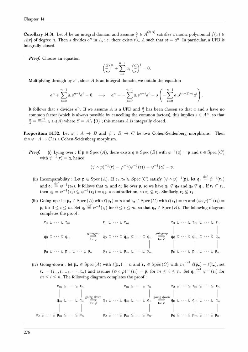
Chapter 14
Corollary 14.31. Let A be an integral domain and assume as ∈ A
Q(A)satisfies a monic polynomial f(x) ∈
A[x] of degree n. Then s divides an in A, i.e. there exists t ∈ A such that st = an. In particular, a UFD isintegrally closed.
Proof. Choose an equation (as
)n+n−1∑i=0
ai
(as
)i= 0.
Multiplying through by sn, since A is an integral domain, we obtain the equation
an +
n−1∑i=0
aisn−iai = 0 =⇒ an = −
n−1∑i=0
aisn−iai = s
(−n−1∑i=0
ais(n−1)−iai
).
It follows that s divides an. If we assume A is a UFD and as has been chosen so that a and s have no
common factor (which is always possible by cancelling the common factors), this implies s ∈ A×, so thatas = as−1
1 ∈ ιS(A) where S = A \ 0 ; this means A is integrally closed.
Proposition 14.32. Let ϕ : A → B and ψ : B → C be two Cohen-Seidenberg morphisms. Thenψ ϕ : A→ C is a Cohen-Seidenberg morphism.
Proof. (i) Lying over : If p ∈ Spec (A), there exists q ∈ Spec (B) with ϕ−1(q) = p and r ∈ Spec (C)with ψ−1(r) = q, hence
(ψ ϕ)−1(r) = ϕ−1(ψ−1(r)) = ϕ−1(q) = p.
(ii) Incomparability : Let p ∈ Spec (A). If r1, r2 ∈ Spec (C) satisfy (ψ ϕ)−1(p), let q1def= ψ−1(r1)
and q2def= ψ−1(r2). It follows that q1 and q2 lie over p, so we have q1 6⊆ q2 and q2 6⊆ q1. If r1 ⊆ r2,
then q1 = ψ−1(r1) ⊆ ψ−1(r2) = q2, a contradiction, so r1 6⊆ r2. Similarly, r2 6⊆ r1.
(iii) Going-up : let p• ∈ Spec (A) with `(p•) = n and r• ∈ Spec (C) with `(r•) = m and (ψϕ)−1(ri) =
pi for 0 ≤ i ≤ m. Set qidef= ψ−1(ri) for 0 ≤ i ≤ m, so that q• ∈ Spec (B). The following diagram
completes the proof :
r0 · · · rm
q0 · · · qm
p0 · · · pm · · · pn
( (
( (
( ( ( (
going-up=⇒for ϕ
r0 · · · rm
q0 · · · qm · · · qn
p0 · · · pm · · · pn.
( (
( ( ( (
( ( ( (
going-up=⇒for ψ
r0 · · · rm · · · rn
q0 · · · qm · · · qn
p0 · · · pm · · · pn.
( ( ( (
( ( ( (
( ( ( (
(iv) Going-down : let p• ∈ Spec (A) with `(p•) = n and r• ∈ Spec (C) with mdef= `(p•) − `(r•), set
r• = (rm, rm+1, · · · , rn) and assume (ψ ϕ)−1(ri) = pi for m ≤ i ≤ n. Set qidef= ψ−1(ri) for
m ≤ i ≤ n. The following diagram completes the proof :
rm · · · rn
qm · · · qn
p0 · · · pm · · · pn
( (
( (
( ( ( (
going-down=⇒for ϕ
rm · · · rn
q0 · · · qm · · · qn
p0 · · · pm · · · pn.
( (
( ( ( (
( ( ( (
going-down=⇒for ψ
r0 · · · rm · · · rn
q0 · · · qm · · · qn
p0 · · · pm · · · pn.
( ( ( (
( ( ( (
( ( ( (
278

Elementary properties of rings and their modules
Our next goal is to show that given A,B integral domains with A integrally closed, integral morphismsϕ : A→ B are Cohen-Seidenberg morphisms. By Proposition 14.27 and Proposition 14.32, since an integralmorphism ϕ : A → B factors into a surjective morphism ϕ : A → ϕ(A) and an integral extensionϕ(A) ⊆ B, it suffices to show that integral extensions are Cohen-Seidenberg. We therefore focus ourattention on integral extensions, i.e. A is a subring of B and B is integral over A.
Lemma 14.33. Let A ⊆ B be an integral extension of integral domains. Then A is a field if and only if Bis a field.
Proof. ( ⇒ ) Suppose A is field and let b ∈ B \ 0. Since B is integral over A, we have an equationbn +
∑n−1i=0 aib
i = 0. Assume the degree of this polynomial n is minimal, i.e. n > 0 is chosen as smallas possible (note that n = 0 leads to 1 = 0, a contradiction since (0) ∈ Spec (A) 6= ∅). Because B is an
integral domain, we know that a0 6= 0, otherwise b(bn−1 +
∑n−1i=1 aib
i−1)
= 0 and cancelling b gives an
equation of smaller degree. We deduce that
b
(bn−1 +
n−1∑i=1
aibi−1
)= −a0 6= 0,
hence multiplying this equation by −a−10 shows that b−1 = −a−1
0
(bn−1 +
∑n−1i=1 aib
i−1), e.g. b ∈ B×.
Therefore B is a field.( ⇐ ) Let a ∈ A \ 0. Then a−1 ∈ B×, so it remains to show that a−1 ∈ A. Since B is integral over A,we have an equation
(a−1)n +n−1∑i=0
ai(a−1)i = 0
which we can multiply through by an−1 to obtain
a−1 = −n−1∑i=0
aian−i ∈ A.
Corollary 14.34. Let A ⊆ B be an integral extension of integral domains and q ∈ Spec (B) be lying overp ∈ Spec (A). Then p ∈ MaxSpec (A) if and only if q ∈ MaxSpec (B).
Proof. The morphism A→ B → B/q has kernel p, hence gives an integral extension of integral domainsA/p → B/q by Proposition 14.23. Since q (resp. p) is maximal if and only if B (resp. A) is a field, theresult follows from Lemma 14.33.
Note : the next lemma requires some knowledge of field theory and Galois theory.
Lemma 14.35. Let A ⊆ B be integral domains, A integrally closed (in its field of fractions) and let b ∈ Bbe integral over a E A. Then b ∈ L def
= Q(B) is algebraic (i.e. integral) over Kdef= Q(A) and if its minimal
polynomial over K is mbL/K(x) = xn +
∑n−1i=0 aix
i, then a0, · · · , ai ∈√a.
Proof. Since a ⊆ K , b is algebraic over K . Let L′def= SplK(mb
L/K) be the splitting field of mbL/K over
K , so that L′ contains all the Galois conjugates of b. Considering the extension A → K → L′, sinceeach Galois conjugate of b is a root of the polynomial mb
L/K , they are all integral over a. The coefficients
of mbL/K are polynomials in these Galois conjugates, hence are also integral over a by Corollary 14.19 ;
since A is integrally closed, they must lie in√aA =
√a by Corollary 14.19 again.
279

Chapter 14
Theorem 14.36. Let ϕ : A → B be integral. Then ϕ satisfies lying over, incomparability and going-up. IfA and B are integral domains and A is integrally closed (in its field of fractions), ϕ is Cohen-Seidenberg(i.e. also satisfies going-down).
Proof. Without loss of generality, we can assume that A is a subring of B by Proposition 14.32.
(i) Lying over : Let p ∈ Spec (A). Since A \ p ⊆ B is a multiplicative subset, the Ap-module Bp is aring and Ap ⊆ Bp is an integral extension. We have a commutative diagram
A B
Ap Bp.
⊆
⊆ ⊆⊆
Let n ∈ MaxSpec (Bp). By Corollary 14.34, mdef= n ∩ Ap ∈ MaxSpec (Ap) = pAp, hence
m = pAp, so that n ∩ A = p. Letting qdef= n ∩ B, we see that q ∩ A = n ∩ A = p. Therefore
q ∈ Spec (B) lies over p.
(ii) Incomparability : By Proposition 14.28, if q, q′ lie over p, the inclusion A ⊆ B leads to the integralextension of integral domains Ap ⊆ Bp. Since qBp and q′Bp both lie over the maximal idealpAp ∈ Spec (Ap), they are both maximal by Corollary 14.34. Therefore they are either equal ordistinct and not included in each other. By Theorem 8.24, the same is true of q and q′.
(iii) Going-up : by induction, we reduce immediately to the case n = 1 andm = 0, so let p• ∈ Spec (A)and q0 ∈ Spec (B) s in the following diagram :
q0 q1
p0 p1
((
(
in which we are looking for q1 ∈ Spec (B) lying over p1 and strictly containing q0. The inducedmorphism A/p0 → B/q0 is integral by Proposition 14.23, so let q1/q0 ∈ Spec (B/q0) be a primelying over p1/p0 ∈ Spec (A/p0). It follows that q1 ∈ Spec (B) is the prime ideal we were lookingfor.
(iv) Going-down : by induction, we reduce immediately to the case n = 1 and m = 0, so let p• ∈Spec (A) and q1 ∈ Spec (B) as in the following diagram :
q0 q1
p0 p1
(
(
By Proposition 14.26, considering the inclusion A ⊆ Bq1 , it suffices to show that p0Bq1 ∩ A = p0.
The inclusion (⊇) is obvious. For the reverse inclusion, let ydef= b
s ∈ p0Bq1 ∩ A \ 0, so that
b ∈ p0B and s ∈ B \ q1 with Kdef= Q(A) and L
def= Q(B). By Corollary 14.19, b is integral over
p0, so that by Lemma 14.35, its minimal polynomial mbL/K(x) = xn +
∑n−1i=0 pix
i satisfies pi ∈ p0
for i = 0, · · · , n − 1. Since y ∈ A, we have s = by ∈ L with y−1 ∈ K , so the minimal polynomial
of s is obtained via the minimal polynomial of b using the formula msL/K(x) = 1
ynmbL/K(yx) (the
factor 1/yn is to ensure msL/K(x) is monic), so we can write
msL/K(x) = xn +
n−1∑i=0
piyn−i
xi = xn +n−1∑i=0
cixi
280

Elementary properties of rings and their modules
and ciyn−i = pi ∈ p0 ⊆ A. Since s ∈ B \ q ⊆ B and B is integral over A, we see that s is integral
over A. We deduce that ci ∈ A for i = 0, · · · , n− 1 (set adef= A in Lemma 14.35).
Suppose y /∈ p0. By Lemma 14.35 (set adef= p0 this time), since ciyn−i = pi ∈ p0, we have ci ∈ p0,
hence sn ∈ p0, thuss ∈ p0 ⊆ p1B ⊆ q1,
a contradiction. Therefore y ∈ p0.
281

Chapter 15
Primary decomposition
This section deals with the existence of a primary decomposition of ideals (resp. submodules) of a ring(resp. module) as an intersection of ideals (resp. submodules) which we will call primary. We begin withthe case of ideals in a ring since this part can be done over an arbitrary ring, is a good introduction to thetheory and makes the case of modules easier to grasp. In the next section, we will deal with modules ; thetheory becomes a little less flexible but most of the main results applicable to ideals can still be applied tomodules. Finally, the Noether-Lasker theorem proves that finite modules over a noetherian ring are a veryconvenient setting to use the theory of primary decomposition since noetherian rings are Lasker rings andfinite modules over noetherian rings are Lasker modules (c.f. Definition 15.1).
15.1 Primary decomposition of ideals in a ring
Definition 15.1. Let A be a ring, q E A an ideal, M an A-module and N ≤M an A-submodule.
• An ideal q E A is called primary if whenever xy ∈ q, then x ∈ q or yn ∈ q. An equivalentformulation is that ZD(A/q) ⊆ Nil(A/q), that is, every zero-divisor in A/a is nilpotent (note that thereverse inclusion is obvious, so the statement is equivalent to ZD(A/q) = Nil(A/q)).
• Let a E A. A primary decomposition for a is the data of a finite set of primary ideals q1, · · · , qn EA such that
a =
r⋂i=1
qi.
The decomposition q1, · · · , qr of a is called
- irredundant if⋂ri=1 qi (
⋂ri=1j 6=i
qi for 1 ≤ j ≤ r.
- minimal if r = minm ∈ N | a =⋂mi=1 q
′i is a primary decomposition for a.
• A proper ideal a E A is called decomposable if it admits a primary decomposition.
• A ring A in which every proper ideal a E A is decomposable is called a Lasker ring.
Remark 15.2. Let A be a ring.
• Prime ideals p ∈ Spec (A) are obviously primary since ZD(A/p) = 0 = Nil(A/p). Any primary idealq admits a unique minimal primary decomposition q, so primary ideals are decomposable.
282

Elementary properties of rings and their modules
• If a1, · · · , an E A are decomposable with decomposition qi1, · · · , qiri for 1 ≤ i ≤ n, so is⋂ni=1 ai ;
it suffices to take the union of the decompositions of each ideal ai, namely
n⋂i=1
ai =n⋂i=1
ri⋂j=1
qij .
• Given a ∈ A and a E A, considering the element a+ a ∈ A/a, we have
(a : a) = b ∈ A | ba ∈ a = b ∈ A | b(a+ a) = 0 = AnnA(a+ a) ⊇ a.
We have (a : a) 6= a if and only if a+ a is a zero divisor in A/a.
Proposition 15.3. Let q E A be a primary ideal. Then√q ∈ Spec (A) is prime, so by Theorem 3.22, it is
a minimum in V(q), i.e. any other prime ideal p satisfying q ⊆ p satisfies√q ⊆ p.
Proof. If xy ∈ √q, then xnyn = (xy)n ∈ q for some n > 0. If x /∈ √q, then xn /∈ q, so there existsm > 0 such that (yn)m ∈ q. It follows that ynm ∈ q, i.e. y ∈ √q.
Definition 15.4. Let q E A be a primary ideal. If pdef=√q, we say that q is p-primary.
Example 15.5. • In the ring Z, the primary ideals are (0) and (pn) for n > 0 and p a prime number.This is because these are the only ideals with prime radical and it is checked by definition that theseare primary ideals.
• Let k be a field and Adef= k[x, y]. We set p = (x, y)A and q = (x2, y). Since A/q ' k[x]/(x2) and
zero divisors in A/q are multiples of x, every zero divisor in A/q is nilpotent, so q is p-primary. Notethat p2 = (x2, xy, y2) ( q ( (x, y) = p, so a p-primary ideal is not necessarily a prime power.
• Conversely, a prime power is not necessarily primary, even though its radical is prime. For example,let A = k[x, y, z]/(xy − z2) and denote by x, y and z the equivalence classes of x, y and z in A
respectively. Then pdef= (x, z) is prime (since A/p ' k[y] is an integral domain), we have xy = z2 ∈ p2
but we show that x /∈ p2 and y /∈√
p2 = p.
In the first case, since p = (x, z), we have
p2 = (x2, xz, z2) = (x2, xz, xy) = (x)(x, y, z).
Note that the lift of p2 to k[x, y, z] would then be equal to (x2, xy, xz, z2), which still does not containx since it only has zero and polynomials of degree ≥ 2. The lift of p to k[x, y, z] is (x, z) and obviouslydoesn’t contain y ; by the same argument, we conclude that y /∈ p.
Proposition 15.6. Let A be a ring and a E A. If mdef=√a ∈ MaxSpec (A), then a is m-primary. In
particular, the powers of a maximal ideal m ∈ MaxSpec (A) are m-primary.
Proof. By Proposition 15.3, there is only one prime ideal containing a, namely m. Therefore Spec (A/a) =m and m = Nil(A/a). It follows that elements of A are either units or nilpotents, i.e. ZD(A/a) =Nil(A/a), so a is m-primary. The second result follows since
√mn = m for any n > 0.
Proposition 15.7. Let q E A be an ideal. Then q is primary if and only if for every a, b E A satisfyingab ⊆ q, then a ⊆ q or b ⊆ √q.
283
Chapter 15
Proof. (⇒) Suppose there exists a, b E A with ab ⊆ q, a 6⊆ q and b 6⊆ √q. There exists a ∈ a ∩ (A \ q)and b ∈ b∩ (A \√q), so that ab ∈ ab ⊆ q. Since q is primary, a ∈ q or bn ∈ q for some n ≥ 1, i.e. a ∈ qor b ∈ √q, a contradiction.(⇐) Given a, b ∈ A such that ab ∈ q, let a = (a)A and b = (b)B . Then ab = (ab)A ⊆ q, so a ∈ a ⊆ q orb ∈ b ⊆ √q, which implies a ∈ q or bn ∈ q for some n ≥ 1.
Lemma 15.8. Let p ∈ Spec (A) and q1, · · · , qr be p-primary ideals. Then qdef=⋂ri=1 qi is p-primary.
Proof. By Proposition 3.20, we have
√q =
√√√√ r⋂i=1
qi =
r⋂i=1
√qi =
r⋂i=1
p = p.
Suppose x, y ∈ A satisfy xy ∈ q but x /∈ q, so that x /∈ qi for some 1 ≤ i ≤ r. It follows that yn ∈ qi forsome n ≥ 1, i.e. y ∈ √qi = p =
√q. Therefore some power of y lies in q (say ym ∈ q), so q is p-primary
(note that n 6= m in general).
Remark 15.9. By Lemma 15.8, if p1, · · · , pr ∈ Spec (A) and qi1, · · · , qini E A are pi-primary ideals for
1 ≤ i ≤ r and 1 ≤ j ≤ ni, letting qidef=⋂nij=1 qij , we see that
⋂1≤i≤r
1≤j≤ni
qij =
r⋂i=1
qi.
In other words, we can collect the p-primary ideals of a given primary decomposition of an ideal to reducethe number of primary ideals involved in the intersection ; furthermore, the resulting intersection hasprecisely one primary ideal for each prime p ∈ Spec (A) involved in the decomposition. Of course, if aprimary decomposition is minimal, the operation qij 7→ qi will not affect the set of primary idealsinvolved in the decomposition, i.e. ni = 1 for 1 ≤ i ≤ r.
Starting with a primary decomposition q1, · · · , qr for a decomposable ideal a, performing the opera-tion qij 7→ qi gives us a decomposition with precisely one primary ideal per prime which appeared inthe original decomposition ; removing unnecessary primary ideals, we can assume the decomposition thusobtained is irredundant. We will show in Theorem 15.11 that such an irredundant decomposition is minimal.
Lemma 15.10. Let A be a ring, a ∈ A and q E A be a p-primary ideal.
(i) If a ∈ q, then (q : a) = A.
(ii) If a ∈ A \ q, then (q : a) is p-primary, i.e.√
(q : a) = p.
(iii) If a ∈ A \ p, then (q : a) = q.
Proof. Recall (c.f. Remark 15.2) that
(q : a) = b ∈ A | ba ∈ q.
(i) If b ∈ A, then ab ∈ q since q E A, so that A ⊆ (q : a).
(ii) If b ∈ (q : a), then ab ∈ q, so since a /∈ q, bn ∈ q for some n ≥ 1, i.e. b ∈√
(q : a) = p. This givesq ⊆ (q : a) ⊆ p, so taking radicals gives
√(q : a) = p.
(iii) The inclusion q ⊆ (q : a) is clear. Conversely, if b ∈ (q : a), then ab ∈ q, but since a ∈ A \ √q, wemust have b ∈ q.
284

Elementary properties of rings and their modules
Theorem 15.11. Let A be a ring and a E A a decomposable ideal and a =⋂ri=1 qi be a minimal primary
decomposition of a. Set pidef=√qi for 1 ≤ i ≤ r. (Note that by Remark 15.9, the primes p1, · · · , pr are
distinct.) Then √(a : a)
∣∣∣ a ∈ A \ a, √(a : a) ∈ Spec (A)
= p1, · · · , pr.
In particular, the set p1, · · · , pr does not depend on the chosen primary decomposition for a, and foreach 1 ≤ i ≤ r, there exists ai ∈ A with
√(a : ai) = pi. As a corollary, Remark 15.9 builds a minimal
primary decomposition out of a given primary decomposition for any decomposable ideal a.
Proof. For any a ∈ A, by definition of the module quotient and Lemma 15.10, we have
√(a : a) =
√√√√( r⋂i=1
qi : a
)=
√√√√ r⋂i=1
(qi : a) =
r⋂i=1
√(qi : a) =
r⋂i=1qi 63a
pi.
(⊆) This follows from the Prime Intersection Lemma (c.f. Theorem 3.32) since√
(a : a) ∈ Spec (A).
(⊇) Let 1 ≤ j ≤ r. By minimality of the decomposition, there exists aj ∈ (A \ qj) ∩⋂ri=1i 6=j
qi, so that by
Lemma 15.10, √(a : aj) =
r⋂i=1
√(qi : aj) =
√(qj : aj) = pj .
Definition 15.12. Let A be a ring and a E A. The prime ideal p ∈ Spec (A) is said to belong to a if thereexists a ∈ A \ a such that p =
√(a : a) ; equivalently, if p =
√AnnA(a+ a). The set of primes belonging
to a is denoted by BelA(a) (c.f. Definition 15.51). The minimal elements of BelA(a) are called isolatedprimes of a. The other, non-minimal ones are called embedded primes. Theorem 15.11 says that if a E Ais a decomposable ideal and q1, · · · , qr is a minimal primary decomposition for a where qi is pi-primary,then BelA(a) = p1, · · · , pr ; this is because AnnA(a+ a) = (a : a) by Remark 15.2.
Example 15.13. • In the ring Z, given n ∈ Z \0, a primary decomposition of the ideal (m)Z isgiven by its factorization in prime powers m =
∏ni=1 p
aii with ai ≥ 0 and pi pairwise distinct prime
numbers, so that
(m)Z =
n⋂i=1
(paii )Z
is a minimal primary decomposition. Each (pi)Z ∈ Spec (Z) is a maximal ideal (since Z/piZ ' Fpiis a field), hence every prime belonging to (m)Z is isolated. If n = 0, (0) is prime, hence an isolatedprime of itself.
• Let A = k[x, y] where k is a field and set adef= (x2, xy)A. Then a = p1 ∩ p2
2 where p1 = (x) andp2 = (x, y). The ideal p2
2 is p2-primary since (x, y) is maximal, so the set BelA(a) = p1, p2. Sincep1 ⊆ p2, we see that p2 is an embedded prime. Furthermore,
√a =√p1 ∩
√p2
2 = p1 ∩ p2 = p1, buta is not a primary ideal (because xy ∈ a but x /∈ a and yn /∈ a for all n > 0).
• A minimal primary decomposition of an ideal may not be unique : recalling the ideal q = (x2, y)from Example 15.5, we have
(x) ∩ (x, y)2 = (x2, xy) = (x) ∩ (x2, y)
so that (x), (x, y)2 and (x), (x2, y) are two minimal primary decompositions for (x2, xy). Wewill, however, deduce some uniqueness properties in the subsequent results.
285

Chapter 15
• The names “isolated” and “embedded” primes come from algebraic geometry. Given an algebraicallyclosed field k and an ideal a E k[x1, · · · , xn], the zero locus of points x ∈ kn satisfying f(x) = 0for all f ∈ a is called an algebraic set ; the algebraic set of a prime ideal p ∈ Spec (k[x1, · · · , xn])is called an affine variety. It can be shown that the algebraic set associated to a is a finite union ofaffine varieties corresponding to the isolated primes of a ; the other primes belonging to a give rise tovarieties sitting inside the varieties associated to the isolated primes, so we call them embedded.
To really “see” this geometrically, consider the example adef= (xy) E A
def= k[x, y]. The equation
xy = 0 corresponds to x = 0 or y = 0, i.e. the algebraic set associated to the ideal a is the unionof the x-axis and y-axis in k2. Since the ideals (x) and (y) are prime, we see that (xy) = (x) ∩ (y)is a minimal primary decomposition (because (xy) is not primary ; this can be checked directly sincex, y ∈ k[x, y] satisfy xy ∈ a). The algebraic set associated to (x) is the line of equation x = 0, andsimilarly for (y) we associate the line of equation y = 0.
Proposition 15.14. Let A be a ring and a E A be a decomposable ideal. Then AssA(A/a) ⊆ BelA(a). If Ais noetherian, we have equality.
Proof. By Remark 15.2, we have
AssA(A/a) = p ∈ Spec (A) | ∃a ∈ A s.t. p = AnnA(a+ a)
⊆ p ∈ Spec (A) | ∃a ∈ A s.t. p =√
(a : a) =√
AnnA(a+ a)= BelA(a).
For the reverse inclusion in the noetherian case, if a ∈ A is such that√
AnnA(a+ a) ∈ Spec (A),applying Corollary 10.26 shows that AnnA(a+a) ∈ AssA(A/a) ⊆ Spec (A), and in particular AnnA(a+a) is a prime ideal, so it is equal to its own radical. This means
√AnnA(a+ a) = AnnA(a + a) ∈
AssA(A/a), meaning that BelA(a) ⊆ AssA(A/a).
Remark 15.15. Recall Remark 10.27 for an example where the inclusion is strict. Also note that the ideal
adef= (x2
i | i ∈ N)A given there is primary since√a = m ∈ MaxSpec (A), c.f. Proposition 15.6. In
particular, a is decomposable. Since equality holds when A is noetherian, the issue here is the ring, not thedecomposability of the ideal.
Theorem 15.16. Let A be a ring and a E A be a decomposable ideal.
(i) Primes p ∈ Spec (A) which are minimal in V(a) are isolated primes of a. Any prime ideal containinga contains such an isolated prime.
(ii) The set of minimal primes for a (namely, the minimal prime ideals in the set V(a) = suppA(A/a),c.f. Corollary 10.25) agrees with the set of isolated primes of a.
Proof. (i) By the Prime Intersection Lemma (c.f. Theorem 3.32), if p ⊇ a and we choose a minimalprimary decomposition q1, · · · , qn for a where
√qi = pi ∈ BelA(a), then
p =√p ⊇√a =
n⋂i=1
√qi =
n⋂i=1
√pi =
n⋂i=1
pi,
hence p ⊇ pi for some 1 ≤ i ≤ n. Since pi ∈ V(a) and p is minimal in V(a), we have p = pi.By Proposition 3.18, any prime ideal p′ ∈ V(a) contains a minimal prime p ∈ V(a), so the secondpart of the statement follows from the first.
(ii) We know by (i) that minimal primes of V(a) are isolated primes of a. Conversely, if p ∈ BelA(a) isan isolated prime, since p ∈ V(a), it contains a minimal prime p′ ∈ V(a) by Proposition 3.18, andby part (i) p′ is also isolated, so p = p′ is a minimal prime in V(a).
286

Elementary properties of rings and their modules
Proposition 15.17. Let A be a ring and a E A be a decomposable ideal. Then⋃p∈BelA(a)
p = a ∈ A | (a : a) 6= a.
In particular, if the zero ideal is decomposable, we have⋃p∈BelAA(0)
p = ZD(A),
i.e. the set of zero divisors equals the union of the prime ideals belonging to the zero ideal.
Proof. If a is decomposable with minimal primary decomposition q1, · · · , qn, then 0 is decomposablein A/a with minimal primary decomposition q1/a, · · · , qn/a and qi/a is pi/a-primary. If πa : A →A/a denotes the projection, since
π−1a
⋃p∈BelA(a)
p/a
=⋃
p∈BelA(a)
p
andπ−1a (a+ a ∈ A | (0 : a+ a) 6= (0)) = a ∈ A | (a : a) 6= a,
we reduce to the case a = (0), in which case we want to prove that⋃p∈BelAA(0)
p = ZD(A).
In this case, (0 : a) = AnnA(a), hence a ∈ A | (0 : a) 6= (0) = ZD(A). By Proposition 3.25, we seethat ZD(A) =
⋃a∈A\0
√AnnA(a).
(⊆) The result follows since by Theorem 15.11, each p ∈ BelAA(0) has the form√
(0 : a) =√
AnnA(a)for some a ∈ A.
(⊇) By Proposition 3.25, it suffices to show that for all a ∈ A \ 0,√
(0 : a) ⊆⋃
p∈BelAA(0) p. Letq1, · · · , qr be a minimal primary decomposition of 0. If a ∈
⋂ri=1A \ (A \ qi) =
⋂ri=1 qi = (0),
we have nothing to show. Assume a ∈ A \ qi for some 1 ≤ i ≤ r. In the proof of Theorem 15.11, wehave shown that √
(0 : a) =r⋂i=1qi 63a
pi ⊆⋃
p∈BelAA(0)
p.
Remark 15.18. By Theorem 15.16 and Proposition 15.17, for a ring A and a decomposable ideal a E A, wehave
π−1a (ZD(A/a)) =
⋃p∈BelA(a)
p, π−1a (Nil(A/a)) =
⋂p∈BelA(a)
p.
The second equality follows since BelA(a) contains the minimal primes of a. When a = q is p-primary, theminimal primes in V(q) consist of p, so that ZD(A/q) = p/q = Nil(A/q), which we do not need to provesince it follows by definition of a primary ideal ; we can re-write this property as π−1
q (ZD(A/q)) = p =π−1q (Nil(A/q)). We can claim that we generalized this property to the decomposable case.
Lemma 15.19. Let ϕ : A → B be a morphism of rings and assume q E B is p-primary for p ∈ Spec (B).Then ϕ−1(q) is ϕ−1(p)-primary.
287

Chapter 15
Proof. Suppose x, y ∈ A satisfy xy ∈ ϕ−1(q). Then ϕ(x)ϕ(y) ∈ q, thus ϕ(x) ∈ q (i.e. x ∈ ϕ−1(q)) orϕ(y)n ∈ q (i.e. yn ∈ ϕ−1(q)). The second property follows since
√ϕ−1(q) = ϕ−1(
√q) = ϕ−1(p).
Proposition 15.20. Let (A,S) ∈ Loc and q E A be a p-primary ideal where p ∈ Spec (A).
(i) If S ∩ p 6= ∅, then S−1q = S−1A.
(ii) If S∩p = ∅, then S−1q is S−1p-primary and ι−1S (S−1q) = q. Therefore, the map a 7→ S−1a restricts
to a bijection between the primary ideals q E A satisfying√q ∩ S = ∅ and the primary ideals of
S−1A.
Proof. (i) If s ∈ S ∩ p, then sn ∈ S ∩ q for some n ≥ 1, so that sn
1 ∈ S−1q ∩ (S−1A)×.
(ii) The assumption s ∈ S, a ∈ A and as ∈ q implies a ∈ q since sn /∈ q for all n ≥ 1. Consideringthe morphism ιS : A→ S−1A, this implies
ι−1S (S−1q) = qec =
⋃s∈S
(q : s) =⋃s∈S
q = q
by Theorem 8.24. The second conclusion follows since the map S−1 : primary ideals of A →primary ideals of S−1A is injective (by what we just proved) and surjective by Theorem 8.24 andLemma 15.19.
Definition 15.21. Let (A,S) ∈ Loc and a E A an ideal. We let aSdef= ι−1
S (S−1a) be the saturation of awith respect to S. Note that a ⊆ aS = (aS)S by Proposition 4.31 (c.f. Theorem 8.23) and (0)S = ker ιS byTheorem 8.24, so that aS = π−1
a (ker ιπa(S)) = π−1a ((0)S).
Remark 15.22. When q E A is primary and S ⊆ A is multiplicative, we have q ∩ S = ∅ if and only if√q ∩ S 6= ∅. One direction is clear since q ∩ S ⊆ √q ∩ S. For the other, if s ∈ √q ∩ S, there exists n ≥ 1
such that sn ∈ q, but since S is multiplicatively closed, we also have sn ∈ S. By Proposition 15.20, we haveqS ∈ q, A since the equality qS = q is equivalent to q ∩ S = ∅ and qS = A is equivalent to q ∩ S 6= ∅.
Proposition 15.23. Let (A,S) ∈ Loc and a E A be a decomposable ideal satisfying a ∩ S = ∅ (so that
S−1a is a proper ideal of S−1A) with a minimal primary decomposition q1, · · · , qr. Set pidef=√qi and
suppose that the qi are numbered so that S ∩ p1 = · · · = S ∩ pm = ∅ and the sets S ∩ pm+1, · · · , S ∩ prare not empty. Then
S−1a =
m⋂i=1
S−1qi, aS =
m⋂i=1
qi
are minimal primary decompositions. In particular, S−1a and aS are decomposable and forming the setBelA(a) commutes with localization, i.e. S−1BelA(a) = BelS−1A(S−1a).
Proof. We already know that S−1 commutes with finite intersections, so since S−1qm+1 = · · · =S−1qr = S−1A and the ideals S−1q1, · · · , S−1qm are primary by Proposition 15.20, we see thatS−1q1, · · · , S−1qm is a primary decomposition for S−1a (in particular, m ≥ 1 since S−1a 6= S−1A).Since S−1pi = S−1√qi =
√S−1qi are the distinct prime ideals belonging to S−1a for 1 ≤ i ≤ m by
Theorem 15.11, we see that this primary decomposition is minimal. Inverse images via ιS commute withintersections, so (q1)S , · · · , (qm)S = q1, · · · , qm is a primary decomposition for aS (c.f. Proposi-tion 15.20) and BelA(aS) = p1, · · · , pm by Theorem 15.11 applied again, so this decomposition is alsominimal. The equality S−1BelA(a) = BelS−1A(S−1a) is trivial since by Proposition 15.20,
S−1BelA(a) = S−1p1, · · · , pm, pm+1, · · · , pr = S−1p1, · · · , S−1pm = BelS−1A(S−1a).
288

Elementary properties of rings and their modules
Corollary 15.24. Let (A,S) ∈ Loc and a E A. If A is a Lasker ring, then A/a and S−1A are Lasker rings.In particular, the property of a ring being Lasker is stable under localization (c.f. Definition 14.6).
Proof. Primary decompositions of b/a E A/a are in bijective correspondence with primary decomposi-tions of b E A, so the first part is obvious. By Proposition 15.23, if a is decomposable and S−1a is aproper ideal of S−1A, the ideal S−1a is also decomposable, so since every ideal of S−1A has the formS−1a for some a E A decomposable by Theorem 8.24, the result follows.
Definition 15.25. Let A be a ring and a E A an ideal. A subset Σ ⊆ BelA(a) of prime ideals belonging toa is said to be isolated if it satisfies the following condition : if p′ ∈ BelA(a) and p ∈ Σ satisfy p′ ⊆ p, thenp′ ∈ Σ. Set
SΣdef=⋂p∈Σ
(A \ p) = A \⋃p∈Σ
p,
so that SΣ is a multiplicative subset. If p ∈ Spec (A), write Spdef= A \ p.
Theorem 15.26. Let A be a ring, a E A a decomposable ideal with minimal primary decompositionq1, · · · , qr and Σ ⊆ BelA(a) an isolated set of primes. Assume that q1, · · · , qr is ordered so thatΣ = p1, · · · , pm and BelA(a) \ Σ = pm+1, · · · , pr. Then
aSΣ=
m⋂i=1
qi
is independent of the choice of minimal primary decomposition for a.
Proof. By construction of SΣ, p′ ∈ Σ implies p′ ∩ SΣ ⊆ p′ ∩ (A ∩ p) = ∅. By the Prime AvoidanceLemma and Definition 15.25, p′ ∈ BelA(a) \ Σ implies
p′ 6⊆⋃p∈Σ
p =⇒ p′ ∩ SΣ 6= ∅.
It follows that S−1Σ p1, · · · , pr = p1, · · · , pm, so that aSΣ
=⋂mi=1 qi does not depend on the choice
of minimal primary decomposition by Proposition 15.23.
Corollary 15.27. Let A be a ring and a E A be a decomposable ideal. If q1, · · · , qr is a minimal primarydecomposition for a and BelA(a) = p1, · · · , pr, re-ordering the numbering so that p1, · · · , pm is theset of isolated primes of BelA(a), for 1 ≤ i ≤ m, we have qi = aSp . Therefore, qi is uniquely determined bya and does not depend on the choice of primary decomposition. If every prime belonging to a is isolated,it follows that the minimal primary decomposition of a is unique.
Proof. This is straightforward from Proposition 15.23 and Theorem 15.26.
Corollary 15.28. Let A be a ring and a E A be a decomposable radical ideal. Then a has no embeddedprimes, so it admits a unique minimal primary decomposition given by BelA(a), i.e.
a =⋂
p∈BelA(a)
p
is the unique minimal primary decomposition of a.
289
Chapter 15
Proof. If q1, · · · , qr is a minimal primary decomposition with pidef=√qi, then
a =√a =
√√√√ r⋂i=1
qi =
r⋂i=1
√qi =
r⋂i=1
pi.
We deduce that p1, · · · , pr is a minimal primary decomposition, and in particular it is irredundant ;therefore, a has no embedded primes. Unicity of the decomposition follows from Corollary 15.27.
Definition 15.29. Let A be a ring and a E A a decomposable ideal. If q1, · · · , qr is a primary decom-
position and pidef=√qi is an isolated prime for a, the pi-primary ideal qi is uniquely determined by a ; we
call it the pi-primary component of a.
Proposition 15.30. Let (A,S) ∈ Loc and p ∈ Spec (A).
(i) We have (0)Sp = ker(ιp : A→ Ap) and if p′ ⊆ p, then (0)Sp′ ⊇ (0)Sp .
(ii) We have√
(0)Sp ⊆ p, with equality if and only if p is a minimal prime ideal in A.
(iii) If p is a minimal prime ideal of A, then (0)Sp is the minimal p-primary ideal of A (note that p is themaximal p-primary ideal of A since any p-primary ideal q satisfies q ⊆ √q = p).
(iv) We have
a(A)def=
⋂p∈Spec(A)
p minimal
(0)Sp ⊆⋂
p∈Spec(A)
p minimal
p = Nil(A)
and if (0) is decomposable, A has finitely many minimal primes ; furthermore, a(A) = (0) if and onlyif the zero ideal has no embedded primes. (In particular, when A is reduced and 0 is decomposable,a(A) = 0 by Corollary 15.28.)
More generally, if a is decomposable, then it has finitely many minimal prime ideals lying over it, and
π−1a (a(A/a)) =
⋂p∈V(a)
p minimal
aSp
is equal to a if and only if a has no embedded primes, in which case the primary decomposition of ahas p-primary component equal to aSp .
(v) Given a, b E A, we have
(a ∩ b)S = aS ∩ bS , (a + b)S = aS + bS ,√aS = (
√a)S , (ab)S ⊇ aSbS .
(vi) We have aS = A if and only if a ∩ S 6= ∅.
(vii) If S, T ⊆ A are multiplicative subsets, then
(aS)T = aST = (aT )S .
(viii) If a is decomposable, the set
aS | S ⊆ A is a multiplicative subset
is finite.
290

Elementary properties of rings and their modules
Proof. (i) The first part was explained in Definition 15.21. For the second part, it suffices to see thatA \ p ⊆ A \ p′, hence ιp′ factors through ιp, which gives
(0)Sp = ker ιp ⊆ ker ιp′ = (0)Sp′ .
(ii) By definition of a prime ideal and (0)Sp , we have
ker ιp = a ∈ A | ∃s ∈ A \ p s.t. as = 0 ⊆ p =⇒√
ker ιp ⊆√p = p.
(⇒) If p =√
(0)Sp and p′ ∈ Spec (A) satisfies p′ ⊆ p, suppose a ∈ p =√
ker ιp. There existsn ≥ 1 such that an
1 = 0 ∈ p′Ap, and since p′Ap is prime, a1 ∈ p′Ap. Therefore p′Ap = pAp, i.e.p′ = p.
(⇐) If p is a minimal prime ideal, then Spec (Ap) = pAp, hence√(0)Sp =
√ι−1p (S−1(0)) = ι−1
p
(√S−10
)= ι−1
p (Nil(Ap)) = ι−1p pAp = p.
(iii) Since p is a minimal prime, (0)Sp is p-primary by part (ii). If q is a p-primary ideal, then (0) ⊆ qimplies (0)Sp ⊆ qSp = q by Corollary 15.27 since q is a minimal primary decomposition for qand q ∩ Sp = q ∩ (A \ p) = ∅.
(iv) By (ii), for any p ∈ Spec (A) minimal, we have (0)Sp ⊆√
(0)Sp ⊆ p, which gives the inclusion.Assume the zero ideal is decomposable and let q1, · · · , qr be a minimal primary decomposition.
For 1 ≤ i ≤ r, set pidef=√qi. For p ∈ Spec (A) minimal, by part (ii) and the Prime Intersection
Lemma,r⋂i=1
pi =
√√√√ r⋂i=1
qi =√
(0) ⊆√
(0)Sp = p =⇒ pi ⊆ p,
and by minimality of p, we have pi = p ; this means that p ∈ Spec (A) | p is minimal ⊆p1, · · · , pr, which proves the first statement.
If a(A) = 0, then the definition of a(A) is a primary decomposition of 0 by part (ii), thus the set ofminimal primes equals p1, · · · , pr, which means 0 has no embedded primes. Conversely, sincethe primes p1, · · · , pr are isolated primes of 0, they are minimal primes of A, so by part (iii) andCorollary 15.27, we have qi = (0)Spi
. This means
(0) =r⋂i=1
(0)Spi⊇
⋂p∈Spec(A)
p minimal
(0)Sp = a(A).
The case of a E A decomposable reduces to the case where a = 0 by considering the ring A/a.
(v) Recall that aSdef= ι−1
S (S−1a). The first three properties follow from the fact that intersection, sumand radicals commute with the maps a 7→ S−1a and b 7→ ι−1
S (b) for a E A and b E S−1a. As forthe last one, since a 7→ S−1a commutes with products, by Proposition 4.32, we obtain the fourthproperty.
(vi) If a ∩ S 6= ∅, picking a ∈ a ∩ S shows 11 = a
a ∈ S−1a, hence 1 ∈ ι−1
S (S−1a) = aS . Conversely,1 ∈ aS means 1
1 ∈ S−1a, so letting a ∈ a and s ∈ S be such that 1
1 = as , we have t ∈ S such that
ts = ta ∈ a, hence ts ∈ a ∩ S.
(vii) It suffices to prove the first equality since ST = TS. It is not hard to check that for s, t ∈ A, wehave
((a : s) : t) = a ∈ A | ta ∈ (a : s) = a ∈ A | s(ta) ∈ a = (a : st).
291

Chapter 15
By Proposition 2.22 and Theorem 8.24, we have
(aS)T = ι−1T
(T−1
(⋃s∈S
(a : s)
))
= ι−1T
(⋃s∈S
T−1(a : s)
)T−1A
=
(⋃s∈S
(a : s)T
)A
=
(⋃s∈S
⋃t∈T
((a : s) : t)
)A
=
⋃s∈S,t∈T
(a : st)
A
= (aST )A = aST .
(viii) This is straightforward from Proposition 15.23 since if q1, · · · , qr is a primary decomposition fora, then |aS | S multiplicative| ≤ |P(q1, · · · , qr)| ≤ 2r .
Corollary 15.31. Let A be a Lasker ring. Then A has finitely many minimal prime ideals. (This generalizesCorollary 10.25 since the Noether-Lasker Theorem will show that noetherian rings are Lasker rings.)
Proof. This follows from Proposition 15.30 (iv) since the zero ideal is decomposable.
Definition 15.32. Let A be a ring and p ∈ Spec (A). For n ≥ 1, the nth symbolic power of p is defined as
p(n) def= (pn)Sp = ι−1
p (pnAp).
Remark 15.33. As we have seen, the nth power pn of a prime ideal p ∈ Spec (A) is not necessarily p-primary (in fact, there is no reason to believe it is decomposable), so that pn ⊆ p(n) in general. If p′ is aminimal prime lying above pn, then p ⊆ p′, hence p = p′ ; this means that although p is the only minimalprime lying above pn, the ideal pn might have embedded primes (assuming it is decomposable, of course)!The notion of nth symbolic power is there to remedy to this situation, i.e. it is the p-primary component ofpn, since we have seen that the primary component of an isolated prime is uniquely determined by the ideal(c.f. Corollary 15.27) and by definition, p(n) = (pn)Sp .
Proposition 15.34. Let A be a ring, p ∈ Spec (A) and n,m ≥ 1 be integers. Recall the definition ofp-primary component (c.f. Definition 15.29).
(i) The ideal p(n) is p-primary and pnAp = p(n)Ap.
(ii) If pn has a primary decomposition, then p(n) is its p-primary component.
(iii) If p(n)p(m) has a primary decomposition, then p(m+n) is its p-primary component.
(iv) We have pn ⊆ p(n) and pn = p(n) if and only if pn is p-primary.
Proof. (i) By Proposition 15.30, we see that√p(n) = (
√p)Sp = pSp = p. Considering the morphism
ιp : A→ Ap, we havep(n)Ap = (pn)ece = (pn)e = pnAp = (pAp)
n.
292

Elementary properties of rings and their modules
Since pAp is maximal in Ap, p(n)Ap is pAp-primary by Proposition 15.6, so p(n) is p-primary byProposition 15.20.
(ii) Since√pn = p, the prime ideal p is the only minimal prime ideal above p. If it has a primary ideal
decomposition, then (pn)Sp = p(n) is its p-primary component by Corollary 15.27.
(iii) Since√p(n)p(m) =
√p(n) ∩
√p(m) =
√p = p by Proposition 3.20, if p(n)p(m) has a primary
decomposition, by part (i) and Corollary 15.27, its p-primary component equals
(p(n)p(m))Sp = ι−1p ((p(n)Ap)(p
(m)Ap)) = ι−1p ((pnAp)(p
mAp)) = ι−1p ((pn+mAp)) = p(n+m).
(iv) By definition of p(n) def= ι−1
p (pnAp), since ιp(pn) ⊆ pnAp, we have pn ⊆ ι−1p (pnAp) = p(n). If
equality holds, pn = p(n) is p-primary by part (i) ; for the converse, if pn is p-primary, it equals itsown p-primary component, which is p(n) by (ii).
Example 15.35. We recall Example 15.5, where we had shown that if Adef= k[x, y, z]/(xy − z2), then
pdef= (x, z) was such that
p2 = (x2, xz, z2) = (x)(x, y, z) = (x, xy)(x, y, z) = (x, z)(x, y, z).
Letting mdef= (x, y, z) ∈ MaxSpec (A), we have p2 = pm. If q is a primary ideal involved in a primary
decomposition for p2 (so that pm = p2 ⊆ q), then by Proposition 15.7, we have p ⊆ q or m ⊆ √q ; since m ismaximal, m ⊆ √q implies m =
√q. Assuming p is decomposable (which we will prove in Corollary 15.40),
since p2 is not primary and we have shown that p ( BelAA(p2) ⊆ p,m, we have BelAA(p2) = p,m. Aminimal primary decomposition is thus not guaranteed to be unique, and in these cases, we do not have analgorithm yet to compute a primary decomposition.
We finish this subsection with a characterization of Lasker rings.
Definition 15.36. Let A be a ring. The following are two conditions which can be satisfied by A :
(L1) For every proper ideal a E A and every p ∈ Spec (A), there exists a ∈ A \ p such that aSp = (a : a).
(L2) Given a descending chain of multiplicative subsets S1 ⊇ S2 ⊇ · · · ⊇ Sn ⊇ · · · , for every ideal a E A,the corresponding chain of ideals
aS1 ⊆ aS2 ⊆ · · · ⊆ aSn ⊆ · · ·
is stationary (c.f. Definition 9.1).
Lemma 15.37. Let A be a ring satisfying condition (L1). Then A is the intersection of (possibly infinitelymany) primary ideals.
Proof. Let a be a proper ideal of A and let p ∈ V(a) be minimal. Since qdef= aSp1
is p-primary, byLemma 15.10, we can write q = (a : x) for some x ∈ A \ p. We now claim that a = q ∩ (a + (x)).The inclusion (⊆) is obvious. For the converse, suppose q ∈ q satisfies q = a + bx for some a ∈ a andb ∈ A. Since a, q ∈ q, we have bx ∈ q and x ∈ A \ p, thus b ∈ q = (a : x), showing that bx ∈ a, i.e.q = a+ bx ∈ a.
Given a E A, a minimal prime p above a and qdef= aSp , we have just shown that the set
b E A | q ∩ b = a, a ( b 6⊆ p
is not empty (since it contains a + (x) for x ∈ A \ p). If bii≥1 is a chain in this set, then clearly
293
Chapter 15
bdef=⋃i≥1 bi also lies in it, so by Zorn’s Lemma, it admits a maximal element. We denote the choice
of such an ideal by b(a, q), so b(a, q) is maximal with respect to the conditions q ∩ b(a, q) = a anda ( b(a, q) 6⊆ p.
If b(a, q) = A, we have that a = q has a primary decomposition. Otherwise, we can set a0def= a, p1
def= p
be the minimal prime chosen above a0 and q1def= (a0)Sp1
, so that a1def= b(a0, q1) satisfies a0 = q1 ∩ a1.
Repeating this process inductively, assume a0, · · · , ak−1 have been chosen so that pi is a minimal primeabove ai−1, ai 6⊆ pi together with ai−1 = qi ∩ ai for 0 < i ≤ k − 1. By the above, we can let pk be a
minimal prime ideal above ak−1 and set qkdef= (ak−1)Spk
and akdef= b(ak−1, qk). This gives an increasing
chain of idealsa = a0 ( a1 ( · · · ( ak ( ak+1 ( · · ·
satisfying the following properties :
(a) The prime ideals pn | n ≥ 1 are distinct since the inclusion ai ⊆ pj holds precisely when i < j.To see this, it suffices to note that for i < j, we have ai 6⊆ pi (and thus aj 6⊆ pi) but ai ⊆ aj−1 ⊆ pj .
(b) For n > i ≥ 0, we have
ai =
n−1⋂j=i
qj
∩ an.
In particular, a0 =(⋂n−1
j=0 qj
)∩ an.
(c) We can furthermore assume that the an are not the intersection of a family of primary ideals, forotherwise the latter would imply the same for a0 = a, which means our problem is solved.
We repeat the argument by transfinite induction : if α is an ordinal and aββ∈α is an α-chain of properideals of A (i.e. an increasing function α→ Ideal (A)) satisfying the following conditions :
(a) the chain is strictly increasing, i.e. for β, γ ∈ α with β < γ, we have aβ < aγ
(b) for each β ∈ α, we have a minimal prime ideal pβ above aβ and we define qβdef= (aβ)Spβ
; the pβ ’sare distinct. These ideals satisfy the following identity for any β < γ
aβ =
⋂β≤`<γ`∈α
q`
∩ aγ
(c) the ideals aβ are not the intersection of a family of primary ideals of A,
then there exists an ideal aα such that collection of ideals aββ∈α ∪ aα satisfies the same conditions.Namely, we set
a′def=⋃β∈α
aβ, pα minimal above a′, qαdef= (a′)Spα
, aαdef= b(a′, qα).
By construction, for any β ∈ α, we have aβ ⊆ a′ ( aα 6⊆ pα. Then aα ∩ qα = a′ (and the other identitiesfollow by letting γ ∈ α | γ ≥ β play the role of α in the construction).Since A does not contain chains of ideals of arbitrary cardinality (remember that by construction, ourchains were chosen increasing), this leads to a contradiction unless every ideal is the intersection of afamily of primary ideals of A.
294

Elementary properties of rings and their modules
Remark 15.38. Practically speaking, we only need the part of argument which deals with the transfiniteinduction, but we explicited the case of α = ω (i.e. the smallest countable ordinal) because we use it in theproof of Lemma 15.37.
Theorem 15.39. Let A be a ring. Then A is a Lasker ring if and only if A satisfies (L1) and (L2).
Proof. (⇒) Let A be a Lasker ring, p ∈ Spec (A) and a E A an ideal with a given primary decomposition
q1, · · · , qr where pidef=√qi, i.e. qi is pi-primary for 1 ≤ i ≤ r. By Remark 15.22, if we re-order the
primary ideals q1, · · · , qr so that q1, · · · , qm ⊆ p and qm+1, · · · , qr 6⊆ p, then
aSp =r⋂i=1
(qi)Sp =m⋂i=1
qi.
It suffices to show that (m⋂i=1
(A \ pi)
)∩
(r⋂
i=m+1
qi
)∩ (A \ p) 6= ∅,
since by Lemma 15.10, if a is an element in this intersection, then
m⋂i=1
qi =
r⋂i=1
(qi : a) =
(r⋂i=1
qi : a
)= (a : a).
Since qi ⊆ p, A \ p ⊆ A \ pi, this reduces to show that (A \ p) ∩⋂ri=m+1 qi 6= ∅. This follows by the
Prime Intersection Lemma since if⋂ri=m+1 qi ⊆ p, then qi ⊆ p for some m + 1 ≤ i ≤ r, contradicting
the construction. The property (L2) follows by Proposition 15.30 (viii).(⇐) Suppose that A is not a Lasker ring. Return to the construction of Lemma 15.37, where given aproper ideal a E A which does not admit a primary decomposition, we constructed a chain of ideals
a = a0 ( a1 ( · · · ( an ⊆ · · ·
with the properties (a), (b) and (c) listed there. Consider the multiplicative subset Sndef=⋂ni=1(A \ pi) ;
this gives a chain Snn≥1 of multiplicative subsets as in the definition of property (L2). By property (a),
an 6⊆ pj for j ≤ n, so if we pick sj ∈ an∩ (A\pj), sdef=∏nj=1 sj ∈ an∩Sn 6= ∅, we see that (an)Sn = A
(since S−1n an 3 s
s = 11 ). We deduce that
a =
(n⋂i=1
qi
)∩ an =⇒ aSn =
(n⋂i=1
(qi)Sn
)∩ (an)Sn =
n⋂i=1
qi.
Since the chain of ideals aSnn≥1 stabilizes, there exist n such that for all m ≥ n, aSn = aSm , i.e.
n⋂i=1
qi = aSn = aSm =
m⋂i=1
qi =⇒ ∀m ≥ n,n⋂i=1
qi ⊆m⋂
i=n+1
qi ⊆ qm.
It follows that ⋃n≥1
an−1 =⋃n≥1
qn ∩ an =
Corollary 15.40. (Noether-Lasker theorem) Every noetherian ring is a Lasker ring.
Proof. Condition (L2) is clearly satisfied. As for condition (L1), ??.
295

Chapter 15
Lemma 15.41. Let A be a noetherian ring and a E A an ideal. Then there exists n ≥ 1 such that
√an ⊆ a ⊆
√a.
Proof. The inclusion a ⊆√a is clear. Write
√a = (a1, · · · , ar). For each 1 ≤ i ≤ r, there exists mi such
that amii ∈ a. Set ndef= 1 +
∑ri=1(mi − 1). It is clear that
√an is generated by the setai11 · · · airr
∣∣∣∣∣∣ i1, · · · , ir ∈ N,r∑j=1
ij = n
When a sum of positive integers satisfies
∑rj=1 ij = n, we must have ij ≥ mj for some 1 ≤ j ≤ r,
otherwise∑r
j=1 ij ≤∑r
j=1mj − 1 = n− 1 < n. Therefore ai11 · · · airr ∈ a, showing that√an ⊆ a.
Theorem 15.42. (Krull Intersection Theorem) Let A be a noetherian ring and a E A a proper ideal.
(i) We have a(⋂
n≥1 an)
=⋂n≥1 a
n.
(ii) The equality⋂n≥1 a
n = 0 holds in three cases :
• a ⊆ Jac(A)
• A is a local ring
• A is an integral domain.
Proof. (i) Let bdef=⋂n≥1 a
n and let q1, · · · , qr be a primary decomposition for ab. The inclusionab ⊆ b is obvious. To show that b ⊆ ab, it suffices to show that b ⊆ q whenever q is a primaryideal containing ab. Suppose this is not the case, so there exists q primary with q ⊇ ab and b 6⊆ q,e.g. x ∈ b ∩ (A \ q). Since ab ⊆ q, for any a ∈ a, we have xa ∈ q and x /∈ q, thus a ∈ √q, whichmeans a ⊆ √q. By Lemma 15.41, since A is noetherian, we have
b ⊆ an ⊆√qn ⊆ q,
a contradiction. Therefore b = ab.
(ii) The case a ⊆ Jac(A) follows from part (i) together with Nakayama’s lemma. If A is a local ring,then Jac(A) = m ⊇ a, so this follows from the first case. Let m be a maximal ideal containing
a. Since⋂n≥1 a
n ⊆⋂n≥1 m
n, we reduce to the case where adef= m is maximal. Assume A is
an integral domain, so that ιm : A → Am is injective (since ker ιm = (0)Sm = a ∈ A | ∃s ∈A \m s.t. sa = 0). Applying the case of a local ring to the ideal mAm E Am, we obtain
⋂n≥1
mn ⊆⋂n≥1
m(n) =⋂n≥1
ι−1m (mnAm) = ι−1
m
⋂n≥1
mnAm
= 0.
15.2 Primary decomposition of submodules of a module
Most of the statements in this section are generalizations of statements already made in Subsection 15.1, so wekeep the proofs short when convenient. It is a good thing that we started with the primary decompositiontheory of ideals first because the primary decomposition theory of modules loses a bit of strength in
296

Elementary properties of rings and their modules
comparison (although it is still extremely useful) ; the main reason is that prime submodules of a module donot satisfy the Prime Intersection Lemma in the same way that prime ideals satisfy it when they contain afinite intersection of ideals, which was a crucial step in most arguments. Another reason is that in the caseof prime ideals, we could localize at the prime to obtain a ring where the prime was maximal ; this becomesimpossible for modules since we cannot “localize at submodules” as we did with prime ideals. Because theprimary decomposition theory for modules mostly relies on the primary decomposition theory of ideals, itis also relevant to have proven the results concerning it beforehand.
Definition 15.43. Let A be a ring, M an A-module and N ≤ M a submodule. Recall (c.f. Definition 5.1)that ZDA(M) =
⋃m∈M\0AnnA(m).
• An element a ∈ A is called nilpotent in M if there exists n ≥ 1 such that an ∈ AnnA(M), i.e.anm = 0 for all m ∈M . The set of all nilpotents in M is denoted by
NilA(M)def= a ∈ A | ∃n ≥ 1, an ∈ AnnA(M) =
√AnnA(M) =
√(0 : M).
In particular, note that NilA(A) = Nil(A).
• A proper submodule N M is called a prime submodule if ZDA(M/N) ⊆ AnnA(M/N). Notethat we always have AnnA(M/N) ⊆ ZDA(M/N), so for a prime submodule, we have equality. Anequivalent definition is that if a ∈ A, m ∈M \N satisfy am ∈ N , then aM ⊆ N .
• A proper submodule N M is called a primary submodule if ZDA(M/N) ⊆√
AnnA(M/N) =NilA(M/N). Note that we always have NilA(M/N) ⊆ ZDA(M/N) ; if n ≥ 1, an−1M 6⊆ Nbut anM ⊆ N , there exists m ∈ M such that an−1(m + N) 6= 0 and an(m + N) = 0, so thata ∈ AnnA(an−1m + N) ⊆ ZDA(M/N). Therefore, for a prime submodule, we have NilA(M/N) =ZDA(M/N). An equivalent definition of primary submodule is that if a ∈ A,m ∈ M \ N satisfyam ∈ N , there exists an integer n ≥ 1 such that anM ⊆ N .
• A submodule N ≤ M is called a maximal submodule if M/N is a simple module (c.f. Defi-nition 9.13), i.e. if N M and there are no submodules N ′ of M satisfying N N ′ M .Equivalently, N is maximal in the set of proper submodules of M .
• The A-radical of N in M is the ideal radMA (N) E A defined by
radMA (N)def=√
(N : M) =√
AnnA(M/N) = a ∈ A | ∃n ≥ 1 s.t. anM ⊆ N.
If (N : M) = AnnA(M/N) E A is a radical ideal, we say that N is an A-radical submodule of M .Note that if a E A, then radAA(a) agrees with the original definition of the radical
√a of an ideal in a
ring.
• The M-radical of N is the submodule of M defined by
M√N
def=
⋂N≤P≤MP prime
P.
In the case where N is contained in no prime submodule of M , we set M√N
def= M . Note that for
q E A, we have A√q =
√AnnA(A/q) =
√q by Theorem 3.22. A submodule N M is called
M-radical if N = M√N . Note that prime submodules of M are trivially M -radical.
• A primary decomposition for a proper submodule N M is the data of a finite set of primarysubmodules Q1, · · · , Qr ≤M such that
N =r⋂i=1
Qi.
The decomposition Q1, · · · , Qr of N is called
297

Chapter 15
- irredundant if⋂ri=1Qi (
⋂ri=1j 6=i
Qi for 1 ≤ j ≤ r.
- minimal if r = mins ∈ N | N =⋂si=1Qi is a primary decomposition for N.
• A proper submodule N M is called decomposable if it admits a primary decomposition.
• An A-module M in which every proper submodule N M is decomposable is called a Laskermodule.
Lemma 15.44. LetM be an A-module and P be a prime submodule. If a ∈ A,m ∈M \P satisfy anm ∈ Pfor some n ≥ 1, then am ∈ P . In particular, if anM ⊆ P , then aM ⊆ P .
Proof. Let n be minimal with respect to the condition that anm ∈ P . If n > 1, then an−1m ∈ M \ Pand a(an−1m) = anm ∈ P , thus aM ⊆ P , and in particular am ∈ P , a contradiction.
Remark 15.45. Let A be a ring andM an A-module. If N is a maximal submodule ofM , then it is a primesubmodule. To prove this, note that the quotient M/N is a simple A-module, thus isomorphic to A/mwhere m ∈ MaxSpec (A). It follows that ZDA(A/m) = m = NilA(A/m), hence N is a prime submoduleof M . However, Krull’s theorem does not work for modules, i.e. not every submodule is contained in amaximal submodule of M (we will see shortly that it works in the noetherian case, c.f. Proposition 15.46).Therefore, it is not clear that a proper submodule always contains a prime submodule at all.
A great example of this is given in Remark 10.38. We show that the set of prime Z-submodules (i.e.
prime “subgroups”) of G(p) is empty. If n ≥ 0, we have p · 1pn+1 = 1
pn ∈ G(p)n , yet the multiplication by pn
map gives an isomorphism G(p)/G(p)n ' G(p), so that in particular ZDZ(G(p)/G
(p)n ) = ZDZ(G(p)) = pZ
and AnnZ(G(p)/G(p)n ) = AnnZ(G(p)) = 0. Note that this example is a non-noetherian Z-module.
Proposition 15.46. Let A be a ring and M a noetherian A-module. Any proper submodule N M iscontained in a maximal submodule of M .
Proof. Let ΦM,Ndef= N ′ M be the set of proper submodules ofM . The set ΦM,N is not empty since
it contains N . If Nii≥1 is an increasing chain in ΦM,N , sinceM is noetherian,⋃i≥1Ni = Ni0 ∈ ΦM,N
for some i0 ∈ N+. Therefore Zorn’s Lemma applies.
Proposition 15.47. Let M be an A-module and Q M be a primary submodule of M .
(i) The ideal (Q : M) E A is primary, e.g. pdef= radMA (Q) =
√(Q : M) is a prime ideal. We say that Q
is p-primary. If Q is a prime submodule, then (Q : M) E A is also prime.
(ii) The submodule Pdef= M√Q ≤ M is prime if and only if Q contains at least one prime submodule of
M (which is the case ifM is noetherian, c.f. Proposition 15.46) ; otherwise, M√Q = M . If P M , we
say that Q is P -primary. Any prime submodule of M containing Q contains P .
When Q is primary with pdef= radMA (Q) ∈ Spec (A) and P
def= M√Q M , we say that Q is (p, P )-primary.
Proof. (i) Suppose ab ∈ (Q : M) = AnnA(M/Q). If b /∈ AnnA(M/Q), there exists m ∈M \Q withbm ∈ M \ Q. Since a(bm) ∈ Q and Q is primary, this means a ∈ ZDA(M/Q) ⊆ NilA(M/Q),hence there exists n ≥ 1 such that an ∈ AnnA(M/Q). By Proposition 15.3, p =
√(Q : M) is
prime. If P is prime, then it is primary, hence by Lemma 15.44, (P : M) =√
(P : M) is prime.
(ii) Suppose Q contains at least one prime submodule of M , a ∈ A, m ∈ M \ P and am ∈ P . LetP ′ ≤ M be a prime submodule containing Q but not m, i.e. m ∈ M \ P ′ ⊆ M \ Q. Since Q
298

Elementary properties of rings and their modules
is primary, there exists n ≥ 1 such that anM ⊆ Q. By Lemma 15.44, if P ′′ is an arbitrary primesubmodule containing Q, we have anM ⊆ Q ⊆ P ′′, hence aM ⊆ P ′′, which means aM ⊆ P . Thelast statement follows by definition of M
√Q.
Proposition 15.48. Let A be a ring, M an A-module and N ≤M an A-submodule.
(i) We haveM√
M√N = M
√N .
(ii) If ϕ : M →M ′ is a morphism of A-modules and P ≤M ′ is a prime (resp. primary) submodule, thenϕ−1(P ) ≤M is a prime (resp. primary) submodule.
(iii) If ϕ : M →M ′ is a morphism of A-modules and N ′ M ′, then
(N ′ : M ′) ⊆ (ϕ−1(N ′) : M), radM′
A (N ′) ⊆ radMA (ϕ−1(N ′)), M√ϕ−1(N ′) ⊆ ϕ−1
(M′√N ′).
(iv) If N1 ⊆ N2, then M√N1 ⊆ M
√N2 and radMA (N1) ⊆ radMA (N2).
(v) If N1, N2 ≤M , we have M√N1 ∩N2 ⊆ M
√N1∩ M
√N2 and radMA (N1∩N2) = radMA (N1)∩radMA (N2).
(vi) We have M√
M√N1 + M
√N2 ⊆ M
√N1 +N2 and
√radMA (N1) + radMA (N2) ⊆ radMA (N1 +N2).
(vii) Every submodule N of M containing at least one prime submodule of M contains a minimal primesubmodule of M . In particular, if P is a prime submodule of M , then it contains a minimal primesubmodule.
(viii) The A-radical commutes with localization, i.e. if S ⊆ A is a multiplicative subset, then
S−1radMA (N) = radS−1M
S−1A (S−1N).
Proof. (i) It suffices to show that if P M is a prime submodule, then N ≤ P if and only ifM√N ≤ P , which is obvious by the definition of M
√N .
(ii) Suppose a ∈ A and m ∈ M \ ϕ−1(P ) satisfy am ∈ ϕ−1(P ), so that ϕ(am) = aϕ(m) ∈ P .Since ϕ(m) ∈ M ′ \ P , if P is prime, we have aM ′ ⊆ P , e.g. aM = aϕ−1(M ′) ⊆ ϕ−1(P ), soϕ−1(P ) is prime. If P was assumed primary instead, there exists n ≥ 1 such that anM ′ ⊆ P , e.g.anM = anϕ−1(M ′) ⊆ ϕ−1(P ).
(iii) For the first inclusion, consider the following commutative diagram with exact rows :
0 ϕ−1(N ′) M M/ϕ−1(N ′) 0
0 N ′ M ′ M ′/N ′ 0
ϕ ϕ ϕ
By construction, ϕ is injective, hence
(N ′ : M ′) = AnnA(M ′/N ′) ⊆ AnnA(M/ϕ−1(N ′)) = (ϕ−1(N ′) : M).
By taking radicals, we obtain the second inclusion. By part (ii), we have
M√ϕ−1(N ′) =
⋂ϕ−1(N ′)≤P≤M
P prime
P ⊆⋂
N ′≤P ′≤M ′P ′ prime
ϕ−1(P ′) = ϕ−1
⋂N ′≤P ′≤M ′P ′ prime
P
= ϕ−1(M′√N ′).
299
Chapter 15
(iv) This follows by definition in the first case. For the second case, if a ∈ A satisfies aM ⊆ N1, thenaM ⊆ N2, so that (N1 : M) ⊆ (N2 : M). Taking radicals gives the inclusion.
(v) The inclusion follows by (iv) since N1 ∩ N2 ⊆ N1, N2 implies M√N1 ∩N2 ⊆ M
√N1,
M√N2, hence
the result. For the equality, the inclusion (⊆) follows by (iv) since N1∩N2 ⊆ N1, N2. For the reverseinclusion, the composition
M∆−−−−−→M ⊕M
πN1⊕πN2−−−−−−−−−−→M/N1 ⊕M/N2
(where ∆(m)def= (m,m) and πNi(m)
def= m+Ni) has kernel equal to N1∩N2, so thatM/(N1∩N2)
is a submodule of M/N1 ⊕M/N2. We deduce that
AnnA(M/N1) ∩AnnA(M/N2) = AnnA(M/N1 ⊕M/N2) ⊆ AnnA(M/(N1 ∩N2)).
Since taking radicals of ideals commutes with intersections (c.f. Proposition 3.20), we deduce thatradMA (N1) ∩ radMA (N2) ⊆ radMA (N1 ∩N2).
(vi) By (iv), we have M√N1,
M√N2 ⊆ M
√N1 +N2, hence M
√N1 + M
√N2 ⊆ M
√N1 +N2. Since
M√N1 +N2 is M -radical, we obtain the result. A similar argument shows the second inclusion.
(vii) The set ΨM,N = P ′ ≤ M | P ′ prime is non-empty by assumption. Given a decreasing chainPn of prime submodules contained in N , their intersection is also prime. To see this, set
Pdef=⋂n≥1 Pn and assume a ∈ A and m ∈M \ P such that am ∈ P . Let
(viii) This follows by Theorem 8.24 since
S−1radMA (N) = S−1√
(N : M) =√S−1(N : M) =
√(S−1N : S−1M) = radS
−1MS−1A (S−1N).
Lemma 15.49. Let A be a ring, M an A-module and Q1, · · · , Qr M be (p, Pi)-primary submodules of
M . Then Qdef=⋂ri=1Qi is a (p, M
√Q)-primary submodule of M and M
√Q ⊆
⋂ri=1 Pi.
Proof. By Proposition 15.48 (v), we have
radMA (Q) = radMA
(r⋂i=1
Qi
)=
r⋂i=1
radMA (Qi) =
r⋂i=1
p = p
andM√Q ⊆
r⋂i=1
M√Qi =
r⋂i=1
Pi.
Assume a ∈ ZDA(M/Q), so that there exists m ∈ M \ Q =⋃ni=1M \ Qi with am ∈ Q ⊆ Qi for all
1 ≤ i ≤ n. Choose i so that m ∈M \Qi. Since am ∈ Qi and ZDA(M/Qi) ⊆ NilA(M/Qi), we deducethe existence of n ≥ 1 such that an ∈ AnnA(M/Qi), which implies
a ∈√
AnnA(M/Qi) = M√Qi = p = M
√Q =
√AnnA(M/Qi),
so a ∈ NilA(M/Q). This proves Q is a p-primary submodule of M .
Remark 15.50. Lemma 15.49 is sharp. For example, if A is a field and M is a finite-dimensional vectorspace, every proper subspace Q is a prime A-submodule since ZDA(M/Q) = 0 = AnnA(M/Q). LettingQ1, · · · , Qr be subspaces which intersect in zero, we see that 0 = M
√0 =
⋂ri=1
M√Qi. Also note that
300

Elementary properties of rings and their modules
although each Qi is (0)-primary (where (0) E A), we have Pi = M√Qi = Qi, and the Qi are distinct.
Therefore, two p-primary submodules of M are allowed to be P1-primary and P2-primary for differentprime submodules P1, P2.
We also see that the notion of being p-primary is better behaved than the notion of being P -primarywhere p ∈ Spec (A) and P M is a prime submodule, so the following results rely more on the formernotion than on the latter. One of the reasons the A-radical behaves better than the M -radical is that aprime submodule containing the intersection of two prime submodules does not necessarily contain one ofthem, whereas a prime ideal containing the intersection of two prime ideals also contains their product, thuscontains one of the factors.
The technique shown in Remark 15.9 shows that any primary decomposition for a decomposable sub-module gives rise to an irredundant primary decomposition with prime ideals radMA (Q1), · · · , radMA (Qr)which are distinct; Theorem 15.53 will then show that this decomposition is minimal.
Definition 15.51. Let A be a ring, M an A-module, N ≤M a submodule and p ∈ Spec (A).
(i) We say that p belongs to M if there exists m ∈M such that
p = a ∈ A | ∃n ≥ 1 s.t. anm = 0 =√
AnnA(m).
The set of all primes belonging to M is denoted by BelA(M).
(ii) We say that p belongs to the submodule N in M if there exists m ∈M such that
p = a ∈ A | ∃n ≥ 1 s.t. anm ∈ N =√
(N : m) =√
AnnA(m+N).
The set of all primes belonging to N in M is denoted by BelMA (N). Note that BelMA (N) =
BelM/NA (0) = BelA(M/N), so we can reduce arguments involving primes belonging to N in M
to the case where N = 0.
Note that according to Definition 15.12, BelAA(a) = BelA(A/a).
Lemma 15.52. Let A be a ring, M an A-module, Q M a p-primary submodule of M and m ∈ M , sothat p =
√(Q : M) (c.f. Proposition 15.47).
(i) If m ∈ Q, then (Q : m) = A.
(ii) If m ∈M \Q, then (Q : m) is p-primary, e.g.√
(Q : m) = p ∈ BelMA (Q).
Proof. (i) This is just the fact that Q ≤M is a submodule.
(ii) Let a ∈ (Q : m), so that am ∈ Q. Since m ∈M \Q, this means a ∈ ZDA(M/Q) ⊆ NilA(M/Q),so there exists n ≥ 1 such that an ∈ AnnA(M/Q), i.e. a ∈
√AnnA(M/Q) =
√(Q : M) = p.
Since (Q : M) ⊆ (Q : m) ⊆ p (because aM ⊆ Q implies am ∈ Q), taking radicals, we obtain√(Q : m) = p.
Theorem 15.53. Let A be a ring,M an A-module and N a decomposable submodule ofM with a minimalprimary decomposition Q1, · · · , Qr where Qi is pi-primary and the primes p1, · · · , pr are distinct (c.f.Remark 15.50). Then BelMA (N) = p1, · · · , pr is independent of the chosen minimal primary decomposi-tion for N .
301

Chapter 15
Proof. For m ∈M , by Lemma 15.52, we have
√(N : m) =
√√√√( r⋂i=1
Qi : m
)=
√√√√ r⋂i=1
(Qi : m) =r⋂i=1
√(Qi : m) =
r⋂i=1
pi.
(⊆) Given p ∈ BelMA (N), pick m ∈ M such that√
(N : m) = p. By the Prime Intersection Lemma (c.f.Theorem 3.32), we see that p = pi for some 1 ≤ i ≤ r.
(⊇) Since the decomposition is minimal, we can pick m ∈ Qi ∩
(⋂rj=1j 6=i
(M \Qj)
), so that by
Lemma 15.52, √(N : m) =
√(Qi : m) ∩
r⋂j=1
j 6=i
A =√
(Qi : m) = pi,
i.e. pi ∈ BelMA (N).
Corollary 15.54. Let A be a ring, M an A-module and N a decomposable submodule of M with minimalprimary decomposition Q1, · · · , Qr where Qi is pi-primary. Then (N : M) E A is a decomposable idealwith minimal primary decomposition (Q1 : M), · · · , (Qr : M) where (Qi : M) is pi-primary, so thatBelMA (N) = BelAA((N : M)). Furthermore, any prime ideal p ⊇ (N : M) contains a minimal prime idealin the set BelMA (N).
Proof. We see that
(N : M) =
(r⋂i=1
Qi : M
)=
r⋂i=1
(Qi : M).
By Proposition 15.47, this is a primary decomposition for (N : M) and√
(Qi : M) = pi. By Theo-rem 15.11, the decomposition is also minimal since the prime ideals p1, · · · , pr are distinct, and by thesame theorem, we obtain BelAA((N : M)) = p1, · · · , pr = BelMA (N).Since BelMA (N) = BelAA((N : M)), the last statement is a consequence of Theorem 15.16.
Definition 15.55. . Let A be a ring, M an A-module and N a decomposable submodule. A minimalelement in the set of primes BelMA (N) is called an isolated prime of N in M . Other primes are calledembedded primes of N in M .
Proposition 15.56. Let (A,S) ∈ Loc, M an A-module and Q ≤ M a p-primary submodule, e.g. p =√(Q : M) ∈ Spec (A).
(i) If S ∩ p 6= ∅, then S−1Q = S−1A.
(ii) If S∩p = ∅, then S−1Q is an S−1p-primary submodule of S−1M and (ιMS )−1(S−1Q) = Q. In otherwords, the Galois connection between submodules of M and submodules of S−1M given by
(N ≤M) 7→ S−1N, (N ′ ≤ S−1M) 7→ (ιMS )−1(N ′)
restricts to a bijection between the set of primary submodules Q of M such that√
(Q : M) ∩ S = ∅and the primary submodules of S−1M (c.f. Theorem 8.23).
Proof. We begin by noting that by Theorem 8.24,
S−1p = S−1√
(Q : M) =√S−1(Q : M) =
√(S−1Q : S−1M).
(i) If S ∩ p 6= ∅, then S−1A = S−1p =√
(S−1Q : S−1M) 3 1, which means S−1M ⊆ S−1Q.
302

Elementary properties of rings and their modules
(ii) By definition, we have
(ιMS )−1(S−1Q) = m ∈M | ∃s ∈ S s.t. sm ∈ Q.
Clearly Q ⊆ (ιMS )−1(S−1Q). If m ∈ M \ Q and s ∈ S satisfies sm ∈ Q, since Q is primary,there exists n ≥ 1 such that snM ⊆ Q, e.g. s ∈
√(Q : M) = p. This contradicts S ∩ p = ∅,
so we deduce Q = (ιMS )−1(S−1Q). Note that by Proposition 15.48, the contraction of a primarysubmodule is primary.
It remains to show that S−1Q is a primary submodule of S−1M ; for if this is done, the Galoisconnection maps primary submodules to primary submodules via both extension and contraction,is injective fromM to S−1M (by the previous paragraph) and surjective (because every submoduleof S−1M has the form S−1Q for some Q ≤M ).
If ms ∈ S−1M \ S−1Q, then m ∈M \Q. If a
s′ ∈ S−1A, ms′′ ∈ S
−1M \ S−1Q satisfy ams′s′′ ∈ S
−1Q,there exists s ∈ S such that s(am) ∈ Q. This implies the existence of n ≥ 1 such that snanM ⊆ Q,i.e. sa ∈
√(Q : M) = p. Since S ∩ p = ∅, we obtain a ∈ p, e.g. a
s′ ∈ S−1p =
√(S−1Q : S−1M),
so that as′S−1M ⊆ S−1Q, i.e. S−1Q is primary.
Definition 15.57. Let (A,S) ∈ Loc, M an A-module and N ≤M a submodule. We let
NMS
def= (ιMS )−1(S−1N) = m ∈M | ∃s ∈ S s.t. sm ∈ N
be the saturation of N in M with respect to S. Note that N ⊆ NMS = (NM
S )MS for the same reasons
as in Proposition 4.31 and 0MS = (ιMS )−1(S−10) = (ιMS )−1(0) = ker ιMS , so that NMS = π−1
N (ker ιM/NS ) =
π−1N (0S), where 0 ≤M/N denotes the zero submodule of the quotient.
Proposition 15.58. Let (A,S) ∈ Loc, M an A-module and N ≤ M a decomposable submodule withprimary decomposition Q1, · · · , Qr satisfying S−1N S−1M . Let BelMA (N) = p1, · · · , pr so thatpi = radMA (Qi). Assume that the primary submodules Qi are numbered so that S∩p1 = · · · = S∩pm = ∅and S meets pm+1, · · · , pr . Then
S−1N =m⋂i=1
S−1Qi, NMS =
m⋂i=1
Qi
are minimal primary decompositions of S−1N and NMS , respectively.
Proof. We already know that S−1 commutes with finite intersections, so since S−1Qm+1 = · · · =S−1Qr = S−1A and the submodules S−1Q1, · · · , S−1Qm are primary by Proposition 15.56, we seethat S−1Q1, · · · , S−1Qm is a primary decomposition for S−1N ; in particular, m ≥ 1 sinceS−1N 6= S−1M . Since S−1pi = S−1radMA (Qi) = radS
−1MS−1A (S−1Qi) are the distinct prime ideals
belonging to S−1N for 1 ≤ i ≤ m, we see that this primary decomposition is minimal. Inverse imagesvia ιS commute with intersections and inverse images of primary submodules are primary by Propo-sition 15.48, so by Proposition 15.56, (Q1)MS , · · · , (Qm)MS = Q1, · · · , Qm is a primary decompo-sition for NM
S and BelMA (NMS ) = p1, · · · , pm, so this decomposition is also minimal. The equality
S−1BelNA (M) = BelS−1M
S−1A (S−1N) is trivial since
S−1BelMA (N) = S−1p1, · · · , pm, pm+1, · · · , pn = S−1p1, · · · , S−1pm = BelS−1M
S−1A (S−1N).
Corollary 15.59. Let (A,S) ∈ Loc, M an A-module and N ≤ M . If M is a Lasker module, then M/Nand S−1M are Lasker modules. In particular, the property of an A-module being Lasker is stable underlocalization (c.f. Definition 14.6).
303

Chapter 15
Proof. Primary decompositions of N ′/N ≤ M/N are in bijective correspondence with primary decom-positions of N ′ ≤ M , so the first part is obvious. By Proposition 15.58, if N ′ is decomposable andS−1N ′ S−1M , then S−1N ′ is also decomposable, so since every submodule of S−1M has the formS−1N ′ for some N ′ ≤M decomposable by Theorem 8.24, the result follows.
Definition 15.60. Let A be a ring, M an A-module and N ≤ M a submodule. Analogously to Defini-tion 15.25, we say that a subset Σ ⊆ BelMA (N) of prime ideals belonging to N inM is isolated if it satisfiesthe following condition : if p′ ∈ BelMA (N) and p ∈ Σ satisfy p′ ⊆ p, then p′ ∈ Σ.
Theorem 15.61. Let A be a ring, M an A-module, N ≤ M a decomposable submodule with minimal
primary decomposition Q1, · · · , Qr and Σ ⊆ BelMA (N) an isolated set of primes. Set pidef=√
(Qi : M)for 1 ≤ i ≤ r. Assume that Q1, · · · , Qr is ordered so that Σ = p1, · · · , pm and BelMA (N) \ Σ =pm+1, · · · , pr. Then
NMSΣ
=m⋂i=1
Qi
is independent of the choice of minimal primary decomposition for N .
Proof. By construction of SΣ (c.f. Definition 15.25), p ∈ Σ implies p ∩ SΣ ⊆ p ∩ (A \ p) = ∅. By thePrime Avoidance Lemma and Definition 15.25, p′ ∈ BelMA (N) \ Σ implies
p′ 6⊆⋃p∈Σ
p =⇒ p′ ∩ SΣ 6= ∅.
It follows that S−1Σ p1, · · · , pr = p1, · · · , pm, so that NM
SΣ=⋂mi=1Qi does not depend on the choice
of minimal primary decomposition by Proposition 15.58.
Corollary 15.62. Let A be a ring, M an A-module and N ≤ M be a decomposable submodule. IfQ1, · · · , Qr is a minimal primary decomposition for N and BelMA (N) = p1, · · · , pr, re-ordering thenumbering so that p1, · · · , pm is the set of isolated primes of BelMA (N), for 1 ≤ i ≤ m, we haveQi = NM
Spi. Therefore, Qi is uniquely determined by N and does not depend on the choice of primary
decomposition. If every prime belonging to N in M is isolated, it follows that the minimal primarydecomposition of N is unique.
Proof. This is straightforward from Proposition 15.58 and Theorem 15.61.
Proposition 15.63. Let (A,S) ∈ Loc, M an A-module, N ≤M a submodule and p ∈ Spec (A).
(i) We have 0MSp= ker(ιMp : M →Mp) and if p′ ⊆ p, then 0MSp′
⊇ 0MSp.
(ii) Given N1, N2 ≤M , we have
(N1 ∩N2)S = (N1)S ∩ (N2)S , (N1 +N2)S = (N1)S + (N2)S , radMA (NS) ⊇ (radMA (N))S .
If M is finitely generated, the last inclusion is an equality.
(iii) If (N : M) ∩ S 6= ∅, then NMS = M . If M is finitely generated, they are equivalent.
(iv) If S, T ⊆ A are multiplicative subsets, then
(NMS )MT = NM
ST = (NMT )MS .
304

Elementary properties of rings and their modules
(v) If N is decomposable, the set
NS | S ⊆ A is a multiplicative subset
is finite.
Proof. (i) The first part was explained in Definition 15.57. For the second part, it suffices to see thatA \ p ⊆ A \ p′, hence ιp′ factors through ιp, which gives
0MSp= ker ιMp ⊆ ker ιMp′ = 0MSp′
.
(ii) Recall that NMS
def= ι−1
S (S−1N). Since intersections and sums commute with the operations N 7→S−1N and N ′ 7→ (ιMS )−1(N ′), we get the first two equalities. For the last, we explicit
radMA (NS) =√
(NMS : M) =
√a ∈ A | aM ⊆ (ιMS )−1(S−1N)
and by Theorem 8.24,
(radMA (N))S =⋃s∈S
((N : M) : s) =⋃s∈Sa ∈ A | (sa)M ⊆ N.
Clearly, (sa)M ⊆ N implies aM ⊆ (ιMS )−1(S−1N). Conversely, suppose M = 〈m1, · · · ,mr〉Aand find s1, · · · , sr such that siami ∈ N . Then s
def=∏ri=1 si is such that sami ∈ N , i.e.
saM ⊆ N , which gives the reverse inclusion.
(iii) If (N : M) ∩ S 6= ∅, picking s ∈ (N : M) ∩ S such that sM ⊆ N , we have m1 = sm
s ∈ S−1N , so
S−1M = S−1N , hence NMS = M . Conversely, supposeM = 〈m1, · · · ,mr〉A and fix s1, · · · , sr ∈
S such that simi ∈ N . It follows that sdef=∏ri=1 si satisfies smi ∈ N , hence sM ⊆ N .
(vii) It suffices to prove the first equality since ST = TS. The definitions say that m ∈ (NMS )MT if there
exists t ∈ T such that there exists s ∈ S such that t(sm) ∈ N and m ∈ NMST if there exist s ∈ S
and t ∈ T with (st)m ∈ N . These are obviously the same definitions.
(viii) This is straightforward from Proposition 15.23 since if Q1, · · · , Qr is a primary decompositionfor a, then |NM
S | S multiplicative| ≤ |P(Q1, · · · , Qr)| ≤ 2r .
305

Chapter 16
Gradations, Filtrations and Completions
16.1 Commutative monoids
Definition 16.1. Let (Λ,+) be a commutative monoid (whose neutral element will be denoted by 0) and Aa ring ; in this section, any commutative monoid will be denoted additively, so we write Λ instead of (Λ,+).A submonoid of Λ is a subset Λ′ ⊆ Λ which becomes a monoid when we restrict the operation of Λ to Λ′,in which case we write Λ′ ≤ Λ. Given an arbitrary subset T ⊆ Λ, we write 〈T 〉Λ for the submonoid of Λgenerated by T , namely the set of all finite sums of elements of T .
Given a morphism of commutative monoids f : Λ1 → Λ2, the (naive) kernel and image of f aredefined in the obvious way, namely
kerfdef= λ1 ∈ Λ1 | f(λ1) = 0Λ2, im f
def= λ2 ∈ Λ2 | f−1(λ2) 6= ∅.
Given a submonoid Λ′ ≤ Λ, we construct the quotient monoid as follows. Two elements x, y ∈ Λ arecalled equivalent modulo Λ′ if there exists λx, λy ∈ Λ′ such that x + λx = y + λy , in which case wewrite x ≡ y (mod Λ′). It is clear that this gives an equivalence relation which respects addition in Λ, thusgiving the quotient set Λ/Λ′ of equivalence classes the structure of a commutative monoid, together with aprojection map πΛ′ : Λ → Λ/Λ′ which is a morphism. It is not hard to show that the category of commu-tative monoids has all kernels and cokernels with the trivial monoid as a zero object, the kernel being theone we defined above and the cokernel being the quotient by the image. We leave those details to the reader.
The monoid Λ is said to be cancellative if for any λ, λ′, ν ∈ Λ, the equation λ + ν = λ′ + ν impliesλ = λ′. Note that if Λ is cancellative and Λ′ ≤ Λ, then Λ′ and Λ/Λ′ are also cancellative (c.f. Theorem 16.11).
Remark 16.2. As in the case of abelian groups, we would like to have an isomorphism theorem for amorphism f : Λ1 → Λ2
Λ1/ ker f ' im f.
However, our current notion of kernel is not good enough to allow such an isomorphism ; it is a well-definedsurjective morphism of monoids, but it is not always injective! The usual argument in the case of groups isthat f(x) = f(y) implies xy−1 ∈ ker f , hence x and y are equivalent modulo ker f . Here is an (important)example where this argument does not simply generalize.
Let f : N⊕n → N be the map defined by (d1, · · · , dn) 7→∑n
i=1 di. We see that ker f = 0 sincethe integers involved are all non-negative. If f(d1, · · · , dn) = f(d′1, · · · , d′n), the n-tuples (d1, · · · , dn) and(d′1, · · · , d′n) need not be equivalent modulo ker f = 0 (i.e. they need not be equal).
Definition 16.3. Let Λ,Λ1,Λ2 be commutative monoids and f : Λ1 → Λ2 be a morphism of monoids.
306

Elementary properties of rings and their modules
(i) A monoidal relation on Λ is an equivalence relation R ⊆ Λ× Λ such that if (λ1, λ2), (µ1, µ2) ∈ R,then (λ1 +µ1, λ2 +µ2) ∈ R. Note that asking the equivalence relation R to be monoidal is equivalentto requiring the set R to be a submonoid of Λ× Λ.
(ii) The kernel relation of f is a relation on Λ1 given by
ker fdef= (λ1, λ2) ∈ Λ1 × Λ1 | f(λ1) = f(λ2).
One easily sees that this relation is reflexive, symmetric and transitive, hence is an equivalence relationon Λ1.
(iii) Let R be a monoidal relation on Λ. The quotient monoid of Λ by R is the set of equivalence classesof Λ by R, which is denoted (as usual) by Λ/R and comes with a canonical map πR : Λ→ Λ/R. Notethat if λ1 ∼ λ2 and µ1 ∼ µ2, the fact that the relation is monoidal implies that λ1 + µ1 ∼ λ2 + µ2,so equivalence classes can be added to give Λ/R a commutative monoid structure and make πR asurjective morphism of monoids.
Example 16.4. Let f : A → B be a morphism of commutative rings. In particular, it is a morphism of(multiplicative!) commutative monoids. The kernel relation associated to the morphism of monoids f is therelation of equivalence modulo the ideal ker f since f(a) = f(a′) if and only if a−a′ ∈ ker f . In particular,multiplication is not what determines this kernel relation, but rather addition!
Theorem 16.5. Let f : Λ1 → Λ2 be a morphism of monoids. A monoidal relation R on Λ1 satisfiesthe following universal property : there exists a unique morphism fR : Λ1/R → Λ2 making the followingdiagram commute if and only if the monoidal relation ker f satisfies ker f ⊆ R :
Λ1 Λ2
Λ1/R
πR
f
fR
Furthermore, the map fker f : Λ1/ ker f → im f is an isomorphism of monoids.
Proof. If fR exists, the commutativity of the diagram gives ker f ⊆ R. Conversely, the commutativityof the diagram forces fR to be constant on R-equivalence classes (which is possible if and only ifker f ⊆ R), in which case we can define a unique map of sets fR : Λ1/R → Λ2 making the trianglecommute. The fact that it is a morphism of monoids follows from the fact that R is a monoidal relationand f is a morphism of monoids.
Denote the ker f -equivalence class of λ ∈ Λ1 by [λ]. Since for λ1, λ2 ∈ Λ, we have
f(λ1) = fker f ([λ1]) = fker f ([λ2]) = f(λ2) =⇒ [λ1] = [λ2],
we deduce that fker f : Λ1/ ker f → im f is injective. Surjectivity is obvious, so it is an isomorphism.
Corollary 16.6. Let Λ,Λ′′ be a monoid, Λ′ be a submonoid, f : Λ → Λ′′ be a morphism of monoids andπΛ′ : Λ→ Λ/Λ′ be the morphism defined in Definition 16.1.
(i) The monoidal relation kerπΛ′ is precisely the relation of equivalence modulo Λ′ defined in Defini-tion 16.1, so that Λ/ kerπΛ′ = Λ/Λ′.
(ii) The ker f -equivalence classes in Λ are of the form f−1(µ) for µ ∈ im f . In particular, kerf is aker f -equivalence class of Λ, so elements of kerf are all ker f -equivalent to 0.
307

Chapter 16
(iii) The monoidal relation induced by the submonoid kerf is contained in ker f (but might not be equalto it).
Proof. (i) This follows from the definition of equivalence modulo Λ′ and the definition of kerπΛ′ .Note that we write an equality sign and not an isomorphism ; this is because they are constructedexactly the same way, just using different words to name them.
(ii) Clear by definition. Note that kerf = f−1(0Λ′′).
(iii) Straightforward from the definition of ker f since for (x, y) ∈ Λ×Λ, the existence of λx, λy ∈ ker f
such that x+ λx = y + λy (i.e. when x ≡ y (mod kerf)) implies f(x) = f(y), i.e. (x, y) ∈ ker f .
Remark 16.7. Not every monoidal relation on a commutative monoid Λ arises from a submonoid Λ′
via kerπΛ′ , as one can see by Remark 16.2 where the morphism f : N⊕n → N is surjective (so thatN⊕n / ker f ' N by Theorem 16.5), but kerf = 0. If a submonoid Λ′ ≤ N⊕n was such that the projectionπΛ′ : N⊕n → N⊕n /Λ′ satisfied kerπΛ′ = ker f , since all the ker f -equivalence classes of elements ofΛ′ ⊆ kerπΛ′ would have to be zero, we would have Λ′ = 0 (which implies kerπΛ′ is the trivial relation, i.e.the equivalence class of λ ∈ N⊕2 is just λ), a contradiction.
Definition 16.8. A subset S ⊆ Λ is said to generate Λ if for any λ ∈ Λ, there is a function n : S → Nsending s to ns and taking only finitely many non-zero values such that λ =
∑∗s∈S nss (recall that a ∗ as
superscript on a summation symbol indicates that although the sum is indexed by infinitely many terms, ithas finitely many non-zero summands). If this function n is uniquely determined by λ, we say that S is abasis for Λ. If S can be chosen finite, Λ is said to be finitely generated. If Λ has a basis, we say it is free.
A commutative monoid in which the only element with an inverse is its identity element 0Λ is called aninverse-free monoid.
Proposition 16.9. Let Λ be a commutative monoid.
(i) If Λ is free, then Λ is inverse-free.
(ii) If Λ is inverse-free, any submonoid Λ′ ≤ Λ is inverse-free.
Proof. (i) Suppose λ1, λ2 ∈ Λ satisfy λ1 + λ2 = 0. Writing λ1 and λ2 over a basis S for Λ so thatλi =
∑s∈S a
iss, we see that a1
s + a2s = 0 for all s ∈ S, whence λ1 = λ2 = 0.
(ii) If λ1, λ2 ∈ Λ′ satisfied λ1 + λ2 = 0, then Λ would not be inverse-free. This gives the result.
Example 16.10. Quotients of free commutative monoids are in general not even inverse-free.
• Let Λ = N⊕2 and Λ′ = 〈(a, b)〉 for some a, b ∈ N not both zero. We give two cases :
(i) If a = 0, then Λ/Λ′ ' N⊕(Z/bZ). If b = 0, we obtain symmetrically Λ/Λ′ ' (Z/aZ)⊕ N.(ii) If (a, b) = (1, 1), then Λ/Λ′ ' Z. To see this, consider the map
f : N⊕2 → Z, f(x, y)def= x− y.
This map is obviously a morphism of monoids. The ker f -equivalence class [(x, y)] of (x, y) ∈N⊕2 is precisely
[(x, y)] =
(d+ f(x, y), d) | d ≥ max0,−f(x, y) if f(x, y) ≤ 0
(e, e− f(x, y)) | e ≥ max0, f(x, y) if f(x, y) ≥ 0.
308

Elementary properties of rings and their modules
This is precisely the set of 〈(1, 1)〉-equivalence classes on N⊕2, so since f is surjective, we obtainthe desired isomorphism.
• Let Λ = N⊕3 and Λ′ = 〈(1, 1, 0)〉. By the previous case, we see that Λ/Λ′ ' Z⊕N.
Theorem 16.11. Let Λ be a cancellative monoid and R be a monoidal relation on Λ. Then Λ/R iscancellative. In particular, if f : Λ → Λ′ is a morphism of monoids and Λ is cancellative, then Λ/ ker f 'im f is cancellative, and if f is surjective, Λ′ is cancellative.
Proof. By considering πR : Λ → Λ/R, it is sufficient to deal with the case of a surjective morphismof monoids f : Λ → Λ′ and R = ker f . Suppose λ′1 = f(λ1), λ′2 = f(λ2) and ν ′ = f(ν) satisfyλ′1 + ν ′ = λ′2 + ν ′. Then f(λ1 + ν) = f(λ2 + ν), so λ1 + ν and λ2 + ν are equivalent. Find µ1, µ2 ∈ Λsuch that µ1 + (λ1 + ν) = µ2 + (λ2 + ν). Since Λ is cancellative, µ1 + λ1 = µ2 + λ2, i.e. λ1 and λ2 areequivalent. It follows that λ′1 = f(λ1) = f(λ2) = λ′2, which completes the proof.
The first thing we will do to deal with the notion of Λ-graded ring defined in Section 16.2 is to constructthe Grothendieck group of a commutative monoid, which will allows us to assume without loss of generalitythat a Λ-graded ring is always graded by an abelian group.
Theorem 16.12. Let Λ be a commutative monoid. There exists an abelian group G(Λ) together with amorphism of monoids ιΛ : Λ → G(Λ) satisfying the following universal property : for any morphism ofcommutative monoids η : Λ→ A where A is an abelian group, there exists a unique morphism η′ : G(Λ)→A making the following diagram commute :
Λ G(Λ)
A
η
ιΛ
η′
Given a morphism η : Λ → Λ′, this defines a unique morphism G(η) : G(Λ) → G(Λ′), turning G into afunctor from the category of commutative monoids to the category of abelian groups and ι(−) into a naturaltransformation from the identity functor to G. If U is the forgetful functor from the category of abeliangroups to that of commutative monoids, this shows that G is left-adjoint with right-adjoint U .
Finally, ιΛ(Λ) generates G(Λ) and the morphism ιΛ : Λ → G(Λ) is injective if and only if Λ iscancellative.
Proof. Consider the direct sum Λ ⊕ Λ, whose operation is addition coordinate-wise, namely (λ1, λ2) +
(µ1, µ2)def= (λ1 + µ1, λ2 + µ2). Define the following equivalence relation on Λ × Λ : two pairs (λ1, λ2)
and (µ1, µ2) are called equivalent if there exists ν ∈ Λ such that
λ1 + µ2 + ν = λ2 + µ1 + ν.
Denote the equivalence class of (λ1, λ2) by [(λ1, λ2)] and the set of equivalence classes by G(Λ). Wedefine an operation on G(Λ) which will turn it into a commutative monoid, namely
[(λ1, λ2)] + [(µ1, µ2)]def= [(λ1 + µ1, λ2 + µ2)].
If it is well-defined, it is automatic that it turns G(Λ) into a commutative monoid with identity element[(0, 0)] (just check the axioms by “adding decorations”, c.f. Remark 1.19). For well-definedness, assume[(λ1, λ2)] = [(λ′1, λ
′2)] and [(µ1, µ2)] = [(µ′1, µ
′2)], so there exists νλ, νµ ∈ Λ with
λ1 + λ′2 + νλ = λ′1 + λ2 + νλ
µ1 + µ′2 + νµ = µ′1 + µ2 + νµ
=⇒ (λ1 + µ1) + (λ′2 + µ′2) + (νλ + νµ) = (λ′1 + µ′1) + (λ2 + µ2) + (νλ + νµ).j
309
Chapter 16
Note that by definition, [(λ, λ)] = [(0, 0)], so [(λ1, λ2)] + [(λ2, λ1)] = [(λ1 + λ2, λ1 + λ2)] = [(0, 0)].Therefore −[(λ1, λ2)] = [(λ2, λ1)] and G(Λ) is an abelian group. Also note that [(λ1, λ2)] = [(λ1, 0)]−[(λ2, 0)], so if ιΛ : Λ → G(Λ) denotes the map λ 7→ [(λ, 0)] (which is a morphism of monoids by theadding decorations argument), the inverse element we “added” in G(Λ) to the element λ ∈ Λ with thisconstruction is the element [(0, λ)].Let η : Λ → A be a morphism of monoids with A an abelian group. The morphism of monoidsΛ ⊕ Λ → A defined by (λ1, λ2) 7→ η(λ1) − η(λ2) maps the entire equivalence class of (λ1, λ2) to
η(λ1) − η(λ2), hence we can define a map of sets η′ : G(Λ) → A via η′([(λ1, λ2)])def= η(λ1) −
η(λ2). It is also a morphism of abelian groups by the adding decorations argument. The correspondingcommutative triangle trivially commutes. As for the uniqueness of η′, the commutativity of the triangleforces η′(ιΛ(λ)) = −η(λ), thus giving the result.As for the functoriality, the commutative square given below is uniquely completed, defining G(η)uniquely :
Λ G(Λ)
Λ′ G(Λ′)
η
ιΛ
G(η)
ιΛ′
and the square shows that ι is natural. The definition of η′ gives the bijection between the collection ofmorphisms Λ→ U(A) and the collection of morphisms G(Λ)→ A, showing that (G, U) form an adjointpair.The fact that ιΛ(Λ) generates G(Λ) follows from the identity [(λ1, λ2)] = [(λ1, 0)] − [(0, λ2)] and theinjectivity property of ιΛ follows by definition of cancellativity.
Remark 16.13. If Λii∈I is a family of commutative monoids, then we have a natural isomorphism
G
(⊕i∈I
Λi
)'⊕i∈I
G(Λi).
This can be seen directly from the construction or from the fact that it is a left-adjoint, thus commutesnaturally with small colimits (which direct sums are). In particular, one easily computes that G(N) = Z,hence G(N⊕n) = Z⊕n.
16.2 Graded rings and graded modules
Definition 16.14. Let Λ be a commutative monoid and A a ring. We say that A is a Λ-graded ring if thereexists a direct sum decomposition of abelian groups
A =⊕λ∈Λ
Aλ
such that for any λ1, λ2 ∈ Λ,
Aλ1Aλ2
def= a1a2 | a1 ∈ Aλ1 , a2 ∈ Aλ2 ⊆ Aλ1+λ2 .
The subset Aλ ⊆ A is called the λ-graded component of A. If A is a ΛA-graded ring and B is a ΛB-graded ring, a graded morphism (η, ϕ) : (ΛA, A)→ (ΛB, B) is a pair where η : ΛA → ΛB is a morphismof monoids and ϕ : A → B is a morphism of rings such that for any λ ∈ ΛA, we have ϕ(Aλ) ⊆ Bη(λ).
When Λdef= ΛA = ΛB and η = idΛA , we speak of a Λ-graded morphism. Graded rings together with
graded morphisms form a category, which we denote by GrCRing. The category of Λ-graded rings withΛ-graded morphisms is a subcategory of GrCRing, which we denote by Λ-GrCRing.
310

Elementary properties of rings and their modules
If A is a Λ-graded ring, an element a ∈ A is called homogeneous if a ∈ Aλ for some λ ∈ Λ ; since thisλ is then unique when λ 6= 0, the function deg :
⋃λ∈Λ\0(Aλ \ 0)→ Λ sending a nonzero homogeneous
element a ∈ Aλ to the element λ ∈ Λ is called the degree map (the degree of 0 ∈ A is left undefined). Bydefinition of a graded ring, it satisfies deg(a1a2) = deg(a1) + deg(a2) for a1, a2 ∈ A homogeneous. WhenA is an integral domain, the set of nonzero homogeneous elements form a submonoid of NZD(A) and thedegree map is a morphism of monoids.
Let A be a Λ-graded ring. A Λ-graded A-module is an A-module M together with a direct sumdecomposition of abelian groups
M =⊕λ∈Λ
Mλ
such that for any λ1, λ2 ∈ Λ,
Aλ1Mλ2
def= am | a ∈ Aλ1 ,m ∈Mλ2 ⊆Mλ1+λ2 .
The subset Mλ ⊆ M is called the λ-graded component of M . Note that since A0Mλ ⊆ Mλ, so Mλ
canonically becomes an A0-module and the direct sum decomposition of M into the Mλ’s is a directsum decomposition of A0-modules. If M is a ΛA-graded A-module and N is a ΛB-graded B-module, agraded morphism is a triple (η, ϕ, ψ) : (ΛA, A,M) → (ΛB, B,N) where (η, ϕ) : (ΛA, A) → (ΛB, B) isa morphism of graded rings and ψ : M → N[A] is a morphism of A-modules such that ψ(Mλ) ⊆ Nη(λ).The category of graded modules together with graded morphisms is denoted by GrMod, the subcategoryof those triples where Λ is fixed and η = idΛ is denoted by Λ-GrMod and those where (Λ, A) is fixedand (η, ϕ) = id(Λ,A) is denoted by (Λ, A)-GrMod. Note that when Λ is fixed and η = idΛ, a Λ-gradedmorphism is a pair (ϕ,ψ) where ϕ is a morphism of rings ϕ : A → B such that ϕ(Aλ) ⊆ Bλ andψ : M → N[A] is a morphism of A-modules such that ψ(Mλ) ⊆ Nλ for all λ ∈ Λ (notice that if N isΛ-graded, so is N[A] with the exact same direct sum decomposition, hence ψ is a (Λ, A)-graded morphism).
If M is a Λ-graded A-module, an element m ∈ M is called homogeneous if m ∈ Mλ for some λ ∈ Λ; since this λ is then unique, the function deg :
⋃λ∈Λ\0(Mλ \ 0)→ Λ sending a nonzero homogeneous
element m ∈ Mλ to the element λ ∈ Λ is called the degree map. By definition of a Λ-graded A-module,it satisfies deg(am) = deg(a) + deg(m) for a ∈ A, m ∈ M homogeneous such that am 6= 0. Similarly, anA-submodule N ≤M is called homogeneous if the inclusion map ιN : N →M is a Λ-graded morphism,meaning that we have a direct sum decomposition
N =⊕λ∈Λ
ι−1N (Mλ) =
⊕λ∈Λ
(N ∩Mλ)
A similar definition gives the notion of homogeneous ideal : a E A is homogeneous if and only if we havea direct sum decomposition
a =⊕λ∈Λ
ι−1a (Aλ) =
⊕λ∈Λ
(a ∩Aλ)
Example 16.15. (i) Let R be a ring and consider the R-algebra Adef= k[x1, · · · , xn]. Then A is a
Nn-graded ring and for all (d1, · · · , dn) ∈ N⊕n, we have an isomorphism of k-modules
R[x1, · · · , xn](d1,··· ,dn) = 〈xd11 · · ·x
dnn 〉R ' R
and a direct sum decomposition
R[x1, · · · , xn] =⊕
(d1,··· ,dn)∈Nn〈xd1
1 · · ·xdnn 〉R.
Given a monomial xd11 · · ·xdnn , we say that (d1, · · · , dn) ∈ Nn is its multidegree, and it is standard
to say that R[x1, · · · , xn] is graded by multidegree when it is given this graded ring structure. The
311

Chapter 16
same ring may admit different gradings ; for instance, a standard choice of grading for R[x1, · · · , xn]is the grading by total degree, namely for d ≥ 0, we set
R[x1, · · · , xn]ddef= 〈xi11 · · ·x
inn | i1, · · · , in ≥ 0, i1 + · · ·+ in = d〉R
=⇒ R[x1, · · · , xn] =⊕d≥0
R[x1, · · · , xn]d.
A morphism of graded R[x1, · · · , xn]-modules graded by multidegree is said to bemultigraded whenit is a graded morphism in (Nn, R[x1, · · · , xn])-GrMod.
(ii) A monomial in the ring R[x1, · · · , xn] is an element f ∈ R[x1, · · · , xn] which can be written asf = xd1
1 · · ·xdnn where d1, · · · , dn ≥ 0 and a ∈ R. An ideal a E R[x1, · · · , xn] is called a monomialideal if it can be generated by monomials. Given a set of generators f1, · · · , fk for a monomial
ideal a, let deg fidef= (di1, · · · , din) be the corresponding multidegree of fi for 1 ≤ i ≤ k. This
gives us a commutative monoid Λdef= Nn /〈deg f1, · · · , deg fk〉. The corresponding quotient ring
R[x1, · · · , xn]/a is then a Λ-graded ring. A first non-trivial example is given by R[x, y] and the ideal(xy), so that R[x, y]/(xy) is a N2 /〈(1, 1)〉-graded ring ; one can recognize via Theorem 16.12 that thequotient monoid N2 /〈(1, 1)〉 is an abelian group isomorphic to Z, so that R[x, y]/(xy) is a Z-gradedring, which is not obvious at first glance but very clear via our construction. Explicitly, the direct sumdecomposition of this ring is given by
R[x, y] = R⊕
⊕n≥1
〈xn〉R
⊕⊕n≥1
〈yn〉R
.(iii) A graded morphism of rings (η, ϕ) : (ΛA, A) → (ΛB, B) can be such that η is non-trivial. For
instance, pick a Z-graded ring A, fix an integer d > 0 and write
A =⊕n∈Z
An, B =⊕n∈Z
Bn, Bndef=
An/d if n/d ∈ Z0 otherwise.
It follows that we have an inclusion map A→ B given by taking the direct sum of the isomorphisms(i.e. equalities) An = Bdn. The gradings are given by ΛA = ΛB = Z, so that taking η : Z→ Z to bemultiplication by d and ϕ : A → B to be the “identity map”, (η, ϕ) : (Z, A) → (Z, B) is a gradedmorphism, called “multiplication of the grading by d”. As a morphism of rings, ϕ is just the identitymap, so what we did is change the grading.
Another instance of this is when (Λ, A) is a graded ring and Λ is a submonoid of another monoid Λ′.Setting Aλ = 0 for λ ∈ Λ′ \ Λ, we automatically see that (Λ′, A) is a graded ring and the inclusion(Λ, A) ⊆ (Λ′, A) is a graded morphism. Similarly,
(iv) Quotient monoids are more tractable than one might think. Let Λ = N⊕n and consider f : Λ → Ndefined by f(d1, · · · , dn)
def=∑n
i=1 di. The quotient monoid Λ/ ker f is isomorphic to N since f issurjective.
An example of (Λ/ ker f)-graded ring would be A[x1, · · · , xn] where A is a ring and writing
A[x1, · · · , xn] =⊕d∈N
∑d1,··· ,dn≥0
d1+···+dn=d
〈xd11 · · ·x
dnn 〉A
,
we obtain a decomposition of A[x1, · · · , xn] as a (Λ/Λ′)-graded ring. See Theorem 16.26 for detailedexplanations. We call this grading the total degree of A[x1, · · · , xn].
312
Elementary properties of rings and their modules
Proposition 16.16. Let Λ be a commutative monoid and (A,M) ∈ Λ-GrMod.
(i) An ideal a E A is homogeneous (i.e. is a Λ-graded submodule of A, or in other words, the inclusionmap is Λ-graded) if and only if
a =∑λ∈Λ
(a ∩Aλ)︸ ︷︷ ︸aλ
.
In other words, a is homogeneous if all the homogeneous components of its elements are also in a.In particular, a is homogeneous if and only if it can be generated by homogeneous elements. Whena is a Λ-graded ideal, A/a is a Λ-graded ring (via the decomposition given below) and we have anisomorphism of Λ-graded rings
A/a =⊕λ∈Λ
(Aλ + a)/a '⊕λ∈Λ
Aλ/aλ
The ring structure on the latter goes as follows : consider the quotient Aλ/aλ as a quotient of abeliangroups and define multiplication of a1 + aλ1 and a2 + aλ2 by a1a2 + aλ1+λ2 , and extend by theA0-bilinearity of this formula.
(ii) An A-submodule N ≤ M is Λ-graded (i.e. is a Λ-graded submodule of M , or in other words, theinclusion map is Λ-graded) if and only if
N =∑λ∈Λ
(N ∩Mλ)︸ ︷︷ ︸Nλ
.
In other words, N is homogeneous if all the homogeneous components of its elements are also inN . In particular, N is homogeneous if and only if it can be generated by homogeneous elements.When N is a Λ-graded submodule, M/N is a Λ-graded A-module and we have an isomorphism ofΛ-graded A-modules
M/N =⊕λ∈Λ
(Mλ +N)/N '⊕λ∈Λ
Mλ/Nλ.
The module structure on the latter goes as follows : addition is performed λ-wise and for a ∈ Aλ1 and
m+Nλ2 ∈Mλ2/Nλ2 , let a(m+Nλ2)def= (am) +Nλ1+λ2 ∈Mλ1+λ2/Nλ1+λ2 . Extend this definition
by A0-bilinearity.
(iii) If f : M → N is a morphism of Λ-graded A-modules, then ker f is a homogeneous submodule ofM , im f is a homogeneous submodule of N and coker f is Λ-graded.
(iv) The sum and intersection of an arbitrary family of homogeneous submodules of M is again homoge-neous.
(v) The annihilator AnnA(M) is a homogeneous ideal of A.
Proof. (i) The inclusion map ιa : a→ A is Λ-graded if and only if the homogeneous component of ais aλ. It follows that ∑
λ∈Λ
a ∩Aλ
is the largest Λ-graded ideal of A contained in a since it contains all the homogeneous elementsof a. Therefore, a is homogeneous if and only if it is equal to that ideal. The second result followsfrom the fact that the map
A→⊕λ∈Λ
Aλ/aλ,∗∑
λ∈Λ
aλ 7→∑λ∈Λ
aλ + aλ
313
Chapter 16
is a surjective morphism of Λ-graded rings and has kernel∑
λ∈Λ aλ = a.
(ii) This follows the same ideas as in part (i), but multiplication in A is replaced by scalar multiplicationof A on M . The details are the same, thus are omitted.
(iii) Because f is a graded morphism, considering the map of A0-modules fλ : Mλ → Nλ, we have
f =⊕λ∈Λ
fλ =⇒ ker f =∑λ∈Λ
ker fλ =∑λ∈Λ
(ker f ∩Mλ).
By part (ii), we deduce that coker f is Λ-graded. Since im f = ker(N → coker f), we see that im fis also a homogeneous submodule of N .
(iv) Let Mii∈I be such a family of homogeneous submodules. Since their sum is generated byhomogeneous elements (i.e. the homogeneous generators of each Mi), it is homogeneous. We nowconsider their intersection. For each i ∈ I , consider the Λ-graded morphism ϕi : M → M/Mi.
Taking their product, we have a morphism ϕ : M → Ndef=∏i∈IM/Mi. The A-module N is
obviously Λ-graded with Nλ =∏i∈I(M/Mi)λ. It follows that kerϕ =
⋂i∈IMi is homogeneous
by part (iii).
(v) An element a annihilates m ∈M if and only if a is in the kernel of the map ϕm : A→M definedby a′ 7→ a′m. Because M is a Λ-graded A-module, writing m =
∑∗λ∈Λmλ, we have
kerϕm =∗⋂
λ∈Λ
kerϕmλ .
It follows thatAnnA(M) =
⋂λ∈Λ
⋂m∈Mλ
kerϕm
is homogeneous by part (iii) and part (iv).
Proposition 16.17. Let Λ be a cancellative commutative monoid and G(Λ) its associated Grothendieckgroup. There is a canonical fully faithful functor G : Λ-GrCRing → G(Λ)-GrCRing which associates
to each Λ-graded ring A a G(Λ)-graded ring G(A) defined as follows : as a ring, we set G(A)def= A. For
[(λ1, λ2)] ∈ G(Λ), we define the grading as
A[(λ1,λ2)]def=
Aλ1 if λ2 = 0
0 if [(λ1, λ2)] /∈ ιΛ(Λ).
It satisfies the following universal property : for any G(Λ)-graded ring B and any morphism of ringsϕ : A → B such that (ιΛ, ϕ) : (Λ, A) → (G(Λ), B) is a graded morphism (i.e. ϕ(Aλ) ⊆ BιΛ(λ) for allλ ∈ Λ), there exists a unique G(Λ)-graded morphism ϕ : G(A)→ B (equal to ϕ as a morphism of rings, ifwe forget the grading) such that the following diagram commutes in GrCRing :
(Λ, A) (G(Λ),G(A))
(G(Λ), B).
(ιΛ,ϕ)
(ιΛ,idA)
(idG(Λ),ϕ)
Given a Λ-graded morphism of Λ-graded rings ψ : A1 → A2, the associated G(Λ)-graded morphismG(ψ) : G(A1)→ G(A2) is simply equal to ψ.
314
Elementary properties of rings and their modules
More generally, if Λ is a cancellative commutative monoid and A is a Λ-graded ring, there is also acanonical functor G : (Λ, A)-GrMod→ (G(Λ),G(A))-GrMod such that if M is a Λ-graded A-module,then G(M) is a G(Λ)-graded G(A)-module equal to M as an A-module and for the grading, we set
M[(λ1,λ2)]def=
Mλ1 if λ2 = 0
0 if [(λ1, λ2)] /∈ ιΛ(Λ).
Proof. This is a very fancy way of saying that we add zeros to the direct sum decomposition, so theproof is omitted. However, it has the nice property of being functorial (in fact, in all cases, G is a left-adjoint to the canonical forgetful functor), which will prove itself useful since it allows us to see Λ-gradedrings as G(Λ)-graded rings without losing any information, so we will sometimes assume without loss ofgenerality that we are grading our rings over abelian groups instead of commutative monoids.
Definition 16.18. Let Λ be a commutative monoid and A a Λ-graded ring. Given a Λ-graded A-moduleM
and λ ∈ Λ, we define the λ-shift of M as the A-module M(λ)def= M but whose grading has been shifted
by λ, namely
∀µ ∈ Λ, M(λ)µdef= Mλ+µ.
Given a morphism (ϕ,ψ) : (A,M) → (B,N) in Λ-GrMod (so that ϕ : A → B is a morphism ofΛ-graded rings and ψ : M → N[A] is a morphism of Λ-graded A-modules), we can shift this morphism
Sλ(ϕ,ψ)def= (ϕ,ψ) : (A,M(λ))→ (B,N(λ)) ; both Sλ(ϕ) and Sλ(ψ) stay exactly the same as ϕ and ψ as
maps of sets, but for µ ∈ Λ, we have
Sλψ(M(λ)µ) = ψ(Mλ+µ) ⊆ Nλ+µ = N(λ)µ.
(The only formal difference between ψ and Sλψ is that they are defined on different Λ-graded modules.)This gives an endofunctor Sλ : Λ-GrMod→ Λ-GrMod.
Proposition 16.19. Let Λ be a commutative monoid. Seeing Λ as a category with one object, the associationλ 7→ Sλ gives a faithful functor S : Λ→ EndCat(Λ-GrMod), i.e. an injective morphism of monoids, henceΛ ' S(Λ). This has the following consequences :
(i) If λ, µ ∈ Λ, then Sλ Sµ = Sλ+µ = Sµ Sλ
(ii) The shift by 0 ∈ Λ is the identity functor
(iii) If λ ∈ Λ is invertible, then Sλ is invertible and S−1λ = S−λ.
(iv) If Λ is an abelian group, then every shift functor is invertible.
Proof. This is all obvious from the fact that for λ, µ, ν ∈ Λ, we have
(Sµ(Sλ(M)))ν = M(λ)(µ)ν = M(λ)ν+µ = Mν+µ+λ = M(µ+ λ)ν = (Sµ+λM)ν .
For faithfulness of the functor, simply consider a non-zero ring A with the trivial grading A = A0 and
the Λ-graded A-module Mdef= A such that Mλ = A is the only non-zero graded component. Since
for µ ∈ Λ, we have Mµ 6= 0 if and only if µ = λ, we see that if λ, µ ∈ Λ satisfy Sλ = Sµ, thenSλM0 = SµM0, so in particular Mλ = Mµ 6= 0, which means λ = µ, i.e. S is injective. Other details areleft to the reader.
Example 16.20. A very useful example of degree shifting is to correctly interpret some maps as gradedmaps by re-arranging the degrees accordingly. For example, if A = k[x1, · · · , xn] is graded by multidegree(c.f. Example 16.15), multiplication by a monomial xd1
1 · · ·xdnn is an A-linear endomorphism of A but not a
315

Chapter 16
graded map ; however, it is a multigraded morphism xd11 · · ·xdnn : A→ A(d1, · · · , dn) since a homogeneous
polynomial of multidegree (e1, · · · , en) multiplied by xd11 · · ·xdnn has a degree equal to (d1+e1, · · · , dn+en),
hence lands exactly in A(d1, · · · , dn)(e1,··· ,en).
More generally, if Λ is a commutative monoid, A a Λ-graded ring and M a Λ-graded A-module, thenmultiplication by the homogeneous element a ∈ Aλ is an A-linear endomorphism M →M(λ).
Definition 16.21. Let Λ be a commutative monoid and λ ∈ Λ. If (Λ, A,M), (Λ, B,N) ∈ Λ-GrMod aretwo Λ-graded modules, a morphism (ϕ,ψ) : (A,M)→ (B,N) in the category Mod of modules is said tobe graded of degree λ if (ϕ,ψ)λ : (A,M) → Sλ(B,N) = (B,N(λ)) is a Λ-graded morphism (the indexλ only indicates the change of codomain since the maps of sets involved are the same).
Proposition 16.22. Let Λ be a commutative monoid and λ, µ ∈ Λ. If (ϕ1, ψ1) : (A1,M1)→ (A2,M2) hasdegree λ and (ϕ2, ψ2) : (A2,M2) → (A3,M3) has degree µ, then their composition (ϕ2 ϕ1, ψ2 ψ1) :(A1,M1)→ (A3,M3) has degree λ+ µ.
Proof. By definition, the morphisms (ϕ1, ψ1)λ : (A1,M1) → (A2,M2(λ)) and (ϕ2, ψ2)µ : (A2,M2) →(A3,M3(µ)) are Λ-graded. Shifting the second morphism by λ, we obtain a Λ-graded morphismSλ(ϕ2, ψ2)µ : (A2,M2(λ))→ (A3,M3(λ+ µ)) ; compositions of Λ-graded morphisms are Λ-graded, so
(ϕ2 ϕ1, ψ2 ψ1)λ+µ = Sλ(ϕ2, ψ2)µ (ϕ1, ψ1)λ
is a Λ-graded morphism, i.e. (ϕ2 ϕ1, ψ2 ψ1) is graded of degree λ+ µ.
Corollary 16.23. We have a category, the category of graded morphisms, denoted by Λ-DegGrMod ;its objects are those of Λ-GrMod and its morphisms are those morphisms in Mod which are graded ofdegree λ for some λ ∈ Λ.
Proof. This follows from Proposition 16.22.
Remark 16.24. Note that this category Λ-DegGrMod is not additive, i.e. a morphism of degree λ and amorphism of degree µ do not add to a graded morphism of degree λ′ for some λ′ ∈ Λ in general. (The issue
is that you lose homogeneity ; just look at a graded ring A and the graded A-module Mdef= A. Pick two
elements a1, a2 ∈ A homogeneous but of different degrees. Multiplication by a1 + a2 is not homogeneousanymore since (a1 + a2)(1) = a1 + a2 is not homogeneous.
In the sequel, we will most of the time assume that Λ is a cancellative commutative monoid, in whichcase we will identify it with its image in G(Λ) in the same way that we identify N as a subset of Z. The nexttheorem explains how frequently this situation happens and how useful it is to theory of graded rings andmodules.
Lemma 16.25. Let Λ be an inverse-free commutative monoid and (A,M) ∈ Λ-GrMod. Let
A+def=
⊕λ∈Λ\0
Aλ, M+def=
⊕λ∈Λ\0
Mλ.
Then A+ is an ideal in A, M+ is an A-submodule of M and we have an isomorphism in Mod :
(A0,M0) ' (A/A+,M/M+).
Proof. We rely on Proposition 16.16. To show that A+ is an ideal, pick a ∈ Aλ and a′ ∈ Aµ where λ ∈ Λand µ ∈ Λ \ 0, so that aa′ ∈ Aλ+µ ⊆ A+ because Λ is inverse-free, hence λ + µ = 0 is impossible.Similarly, M+ is an A-submodule of M . The isomorphism in Mod is given by Proposition 16.16 and the
316

Elementary properties of rings and their modules
given direct sum decompositions.
Theorem 16.26. Let η : Λ → Λ′ be a morphism of commutative monoids and (A,M) ∈ Λ-GrMod, i.e.A is a Λ-graded ring and M is a Λ-graded A-module.
(i) Write
A =⊕λ∈Λ
Aλ =⊕µ∈im η
⊕λ∈f−1(µ)
Aλ
︸ ︷︷ ︸
Aµ
, M =⊕λ∈Λ
Mλ =⊕µ∈im f
⊕λ∈f−1(µ)
Mλ
︸ ︷︷ ︸
Mµ
.
The above direct sum decompositions imply that (A,M) ∈ Λ′-GrMod. This operation is functorial,hence gives functors Π(η) : Λ-GrCRing → Λ′-GrCRing and Π(η) : Λ-GrMod → Λ′-GrMod.Furthermore, Π is functorial from the category of commutative monoids to the category of (small)categories, Cat.
(ii) If Λ and Λ′ are cancellative, the following diagrams of functors commutes :
Λ-GrCRing Λ′-GrCRing
G(Λ)-GrCRing G(Λ′)-GrCRing
Π(η)
G G
Π(G(η))
Λ-GrMod Λ′-GrMod
G(Λ)-GrMod G(Λ′)-GrMod
Π(η)
G G
Π(G(η))
(iii) Assume that Λ′ is inverse-free. The η-subring of A, the η-irrelevant ideal of A, the canonicalη-submodule of M and the η-irrelevant submodule of M are defined respectively as
Aηdef=
⊕λ∈ker η
Aλ, Aη+def=
⊕λ∈Λ\ker η
Aλ, Mη def=
⊕λ∈ker η
Mλ, Mη+
def=
⊕λ∈Λ\ker η
Mλ.
The η-irrelevant ideal of A is an ideal of A, the η-irrelevant submodule of M is an A-submodule ofM , the quotient ring A/Aη+ and the quotient module M/Mη
+ are ker η-graded Aη-modules and wehave an isomorphism in ker η-GrMod :
(Aη,Mη) ' (A/Aη+,M/Mη+).
Proof. (i) Let µi ∈ im η and ai ∈ Aµi for i = 1, 2. We want to show that a1a2 ∈ Aµ1+µ2 . By arguingon each Λ-homogeneous component of a1 and a2, we might as well assume that a1 and a2 areΛ-homogeneous. But then this amounts to the fact that if λ1 ∈ f−1(µ1) and λ2 ∈ f−1(µ2), thenλ1 + λ2 ∈ f−1(µ1 + µ2) because f(λ1 + λ2) = f(λ1) + f(λ2) = µ1 + µ2. The same argumentshows that M is im η-graded. Adding zeros to the components not displayed in the direct sum(i.e. setting Aµ = 0 and Mµ = 0 for µ ∈ Λ′ \ im η), we obtain a Λ′-grading of A and M . For
functoriality, it suffices to see that if Λη→ Λ′
η′→ Λ′′, then for λ′′ ∈ Λ′′, the union
(η′ η)−1(λ′′) = η−1((η′)−1(λ′′)) =⋃
λ′∈(η′)−1(λ′′)
η−1(λ′)
is disjoint.
(ii) By looking at the definition of the functor G : Λ-GrMod → G(Λ)-GrMod, one sees that itis nothing else but Π(ιΛ) where ιΛ : Λ → G(Λ) is the canonical inclusion. The result followsfrom the naturality of ι (as a natural transformation from the identity functor to the functor Gon commutative monoids) and the functoriality of G and Π, i.e. applying the functor Π on the
317
Chapter 16
commutative square
Λ Λ′
G(Λ) G(Λ′).
η
ιΛ ιΛ′
G(η)
(iii) Up to an isomorphism of commutative monoids Λ/ ker η ' im η, this is precisely the im η-gradingof A. By Proposition 16.9, im η is inverse-free, so we can apply Lemma 16.25 and conclude.
Corollary 16.27. Let Λ be a free commutative monoid and A a Λ-graded ring. The following are equivalent :
(i) The ring A is noetherian
(ii) The ring A0 is noetherian and A is finitely generated as an A0-algebra.
(Remark : for those who skipped the chapter on gradings, we reduce to the case of an N-graded ring in theproof, so you can just read the implications.)
Proof. Fix a basis S for Λ ' N⊕S . Define η : N⊕S → N by adding coefficients, i.e.
η(∑∗
s∈S nsS) def
=∑∗
s∈S ns. By Theorem 16.26 (i), the subring A0 is the same under both grad-ings (i.e. that of N⊕S and that of N induced by Theorem 16.26 (i)), so without loss of generality, assumeA is N-graded.
( (ii) ⇒ (i) ) This follows from Hilbert’s basis theorem.
( (i)⇒ (ii) ) The ideal A+ is finitely generated, so A0 ' A/A+ is noetherian. Since A is noetherian, A+ =(a1, · · · , ak)A is finitely generated ; without loss of generality, assume that a1, · · · , ad are homogeneouselements of degree d1, · · · , dk respectively. We argue that the map of A0-algebras Ψ : A0[x1, · · · , xd]→A defined by xi 7→ ai is surjective. It suffices to show that An ⊆ im Ψ for all n ≥ 0. There is nothing toprove for n = 0. Assume n > 0 and pick y ∈ An ⊆ A+, so that we can write y =
∑ki=1 biai. We may
assume that the bi are homogeneous (the sum over 1 ≤ i ≤ k of the homogeneous components of bi ofdegree m− di for m 6= n multiplied by ai land in Am, hence are zero). It follows that bi ∈ Am for somem < n, hence bi ∈ im Ψ by the induction hypothesis, which means y ∈ im Ψ.
Definition 16.28. Let Λ be a commutative monoid and (A,S) ∈ Loc. We say that S is Λ-homogeneousif
S =⋃λ∈Λ
S ∩Aλ.
Proposition 16.29. Let Λ be a cancellative commutative monoid and (A,S,M) ∈ Loc-Mod. Whensumming over G(Λ), we simplify the notation and assume Λ ⊆ G(Λ) is a subset.
(i) The functor L : Loc-Mod→ Loc-Mod induces a functor
LΛ : Λ-Loc-GrMod→ G(Λ)-Loc-GrMod,
i.e. S−1A is G(Λ)-graded, ιS(S) ⊆ S−1A is G(Λ)-homogeneous and S−1M is a G(Λ)-graded
S−1A-module, all this in a functorial way. More explicitly, let Sλdef= S ∩Aλ and for λ1, λ2 ∈ Λ, set
S−1λ1Aλ2
def=as∈ S−1A
∣∣∣ s ∈ Sλ1 , a ∈ Aλ2
⊆ S−1A
S−1λ1Mλ2
def=ms∈ S−1M
∣∣∣ s ∈ Sλ1 ,m ∈Mλ2
⊆ S−1M.
318

Elementary properties of rings and their modules
Then the gradings in S−1A and S−1M are given by
S−1A =⊕
µ∈G(Λ)
∑λ1,λ2∈Λ
λ2−λ1=µ
S−1λ1Aλ2
, S−1M =⊕
µ∈G(Λ)
∑λ1,λ2∈Λ
λ2−λ1=µ
S−1λ1Mλ2
.
In other words, if deg :⋃λ∈ΛAλ → Λ is the function associating its degree to each homogeneous
element, we set deg as = deg a − deg s for a, s homogeneous and obtain the corresponding degree
function of S−1A (and we proceed similarly on M ). This means that for µ ∈ G(Λ),
(S−1A)µdef=
∑λ1,λ2∈Λ
λ2−λ1=µ
S−1λ1Aλ2
, (S−1M)µdef=
∑λ1,λ2∈Λ
λ2−λ1=µ
S−1λ1Mλ2
.
(ii) Given a morphism of cancellative commutative monoids η : Λ → Λ′, the following diagram com-mutes :
Λ-Loc-GrMod G(Λ)-Loc-GrMod
Λ′-Loc-GrMod G(Λ′)-Loc-GrMod,
Π(η)
LΛ
Π(G(η))
LΛ′
which shows that the association Λ 7→ LΛ and η 7→ (Π(η),Π(G(η)) : LΛ → LΛ′) turns L into afunctor from the category of cancellative commutative monoids to the category of (small) categories.
Proof. (i) We begin by showing that S−1M is graded (which will imply that S−1A is graded via thesame argument). Given any m
s ∈ S−1m, write m =
∑∗λ∈Λmλ, so that ms =
∑∗λ∈Λ
mλs lies in our
direct sum decomposition because s ∈ S is homogeneous. Pick an element
∗∑λ1,λ2∈Λ
λ2−λ1=µ
mλ1
sλ2
∈∑
λ1,λ2∈Λ
λ2−λ1∈µ
S−1λ1Mλ2
By putting all the summands mλ1/sλ2 on the same denominator, we can assume that all thedenominators are equal. It follows that the numerator is also homogeneous since the difference indegrees is constant and equal to µ, so an element of this subset can be written in the form
mλ1sλ2
where mλ1 ∈ Mλ1 and sλ2 ∈ Sλ2 . Suppose that an element ms ∈ S
−1M has two representationsas a sum of elements in these summands, i.e.∑
µ∈G(Λ)
mµ
sµ=m
s=
∑µ∈G(Λ)
m′µs′µ.
Note that degmµ − deg sµ = µ (which is what the subscript µ means). Because all the sµ and s′µare homogeneous, putting all these elements on the same denominator allows us to assume thatthey are all equal to a common homogeneous element s ∈ S. This means that without loss ofgenerality, we have to deal with the case where sµ = s = s′µ. This implies the existence of u ∈ Ssuch that
us
∑µ∈G(Λ)
mµ −m′µ
= 0 =⇒ us(mµ −mµ′) = 0.
Therefore mµs =
m′µs , which is what we wanted to prove. It is clear that multiplication preserves
the G(Λ)-degree of homogeneous elements of S−1A and S−1M , so S−1A is a G(Λ)-graded ring
319

Chapter 16
and S−1M is a G(Λ)-graded S−1A-module. To see that LΛ maps Λ-graded morphisms to G(Λ)-graded morphisms, it suffices to see that if (ϕ,ψ) : (A,S,M) → (B, T,N) is a morphism inΛ-Loc-GrMod, then
ϕ(S ∩Aλ) ⊆ ϕ(S) ∩ ϕ(Aλ) ⊆ T ∩Bλwhich then implies that (S−1ϕ)(S−1
λ1Aλ2) ⊆ T−1
λ1Bλ2 and (S−1ψ)(S−1
λ1Mλ2) ⊆ T−1
λ1Nλ2 . Functori-
ality of LΛ follows from that of L.
(ii) We can factor the functor LΛ into two functors according to the following commutative diagram :
Λ-Loc-GrMod G(Λ)-Loc-GrMod G(Λ)-Loc-GrMod
Λ′-Loc-GrMod G(Λ′)-Loc-GrMod G(Λ)-Loc-GrMod
Π(η)
G
Π(G(η))
LΛ
Π(G(η))
G LΛ′
The first square commutes by Theorem 16.26 (ii), and the second square commutes since whetherwe group direct summands of the ring/module to localize before or after localizing does not changethe result.
Lemma 16.30. Let Λ be a free commutative monoid and A a Λ-graded ring. A homogeneous ideal p E Ais prime if and only if for all a, b ∈ A homogeneous with ab ∈ p, we have a ∈ p or b ∈ p.
Proof. If p ∈ Spec (A) is homogeneous, then the condition is trivial. For the converse, we first deal withthe case where Λ = N. Assume that for all a, b ∈ A homogeneous with ab ∈ p, we have a ∈ p or b ∈ pand pick a =
∑ki=0 ai, b =
∑`j=0 bj ∈ p such that ak, b` 6= 0, ab ∈ p and that for some j between 0 and
`, we have bj ∈ A \ p. If we choose j0 maximal with this property, we may replace b by∑j0
j=0 bj because
a
j0∑j=0
bj = ab−∑
j=j0+1
abj ∈ p,
so without loss of generality, assume j0 = `, i.e. b` ∈ A \ p. By induction on k, we show that ai ∈ p forall 0 ≤ i ≤ k. The homogeneous component of ab of degree k + ` is akb` because in the expression
k∑i=0
∑j=0
aibj ,
all the other summands are homogeneous of lower degree. Therefore, ak, b` ∈ A satisfy akb` ∈ p. Ifk = 0, this means a0 ∈ p, so we are done. If k > 0, we deduce that ak ∈ p, hence (a − ak)b ∈ p. Byinduction on k, since the homogeneous components of a− ak have degree ≤ k − 1, we deduce that theyare in p, i.e. a ∈ p.
Next, we deal with the case where Λ has a finite basis, so without loss of generality, assume Λ = N⊕n.Denote the decomposition of A as a Λ-graded ring by
A =⊕
i1,··· ,in≥0
Ai1,··· ,in .
For any (d1, · · · , dn) ∈ N⊕n with d1, · · · , dn > 0, consider the morphism of monoids
Φ : Λ→ N, (i1, · · · , in) 7→ i1 + d1i2 + d1d2i3 + · · ·+ (d1 · · · dn−1)in.
320

Elementary properties of rings and their modules
We have im Φ = N, so according to Theorem 16.26, we see that A is an N-graded ring. Note that if(i1, · · · , in) and (j1, · · · , jn) satisfy ik, jk < dk for 1 ≤ k ≤ n and Φ(i1, · · · , in) = Φ(j1, · · · , jn),reducing modulo d1 shows i1 = j1, reducing modulo d2 shows i2 = j2, and recursively we deduce thatik = jk, which leads to (i1, · · · , in) = (j1, · · · , jn). Therefore, under the im Φ-grading of A, the first
ddef= d1d2 · · · dn homogeneous components of A are precisely those A(i1,··· ,in) for which 0 ≤ ik < dk for
1 ≤ k ≤ n. Given a ∈ A, b ∈ A \ p satisfying ab ∈ p, we can choose d1, · · · , dn large enough so that theΛ-homogeneous components of a, b and ab lie in the set⋃
0≤ik<dk1≤k≤n
Ai1,··· ,in .
We assumed that if a and b were Λ-homogeneous, then a ∈ p. Repeat the argument of the casewhere Λ = N, which works because for all the ring elements involved in the argument, being Λ-homogeneous is equivalent to being N-homogeneous (in other words, Φ induces a total order on the set(i1, · · · , in) ∈ N⊕n | 0 ≤ ik < dk, so that if a (resp. b) has term of “highest degree” ak (resp. b`), thenthe term of “highest degree” in ab is akb`, so the argument still applies). We deduce that a ∈ p.
If Λ has an arbitrary basis S, given a ∈ A, b ∈ A \ p with ab ∈ p, let S′ ⊆ S be the subset of those basiselements s ∈ S for which a homogeneous component of a, b or ab has a non-zero coefficient in front ofs. It follows that 〈S′〉 ⊆ Λ is free with finite basis S′ and a, b and ab (together with their homogeneouscomponents) lie in the subring
AS′def=
⊕λ∈〈S′〉
Aλ,
so to show that a ∈ p, we can apply the argument to the case of a finite basis and pS′def= p ∩ AS′ ∈
Spec (AS′).
Proposition 16.31. Let Λ be a free commutative monoid and A a Λ-graded ring.
(ii) If a E A, then
ahdef=∑λ∈Λ
(a ∩Aλ)
is an ideal of A.
(iii) If p ∈ Spec (A), then ph ∈ Spec (A) is a homogeneous prime ideal.
(iv) The radical of a homogeneous ideal is homogeneous and satisfies√ah =
√ah.
Proof. (i) It is clear that ah is an additive subgroup of A. If a ∈ A and x ∈ ah, write a =∑∗
λ∈Λ aλand x =
∑∗λ∈Λ xλ. Since each xλ belongs to a, the product ax is a sum of homogeneous elements
of a, i.e. belongs to ah.
(ii) By part (i), we know that ph is a homogeneous ideal of A. Because p is prime, we deduce that ph isprime by Lemma 16.30.
(iii) It is clear that if a E A and p ∈ Spec (A), then ah ⊆ ph. Because a is homogeneous, this meansa = ah ⊆ ph, hence
√ah =
√a =
⋂p∈V(a)
p =⋂
p∈V(a)
ph =
⋂p∈V(a)
ph
h
=
⋂p∈V(a)
p
h
=√ah,
the middle equality holding by Proposition 16.16 (iv).
321

Chapter 16
Remark 16.32. I encountered some problems trying to define the localization at f in the general case. Seethe next section for the case where Λ = Z. It sounds useful to define this notion in the general case where(η, ϕ) : (ΛS , S) → (ΛT , T ) is a morphism of graded rings where η : ΛS → ΛT is a morphism of freecommutative monoids and ϕ : S → T is a morphism of rings satisfying ϕ(Sλ) ⊆ Tη(λ) for all λ ∈ ΛS . Theproblem is that I have to interpret what happens to the irrelevant ideal in this context, and this demandsan entire re-interpretation of Proj, which I will not do at the moment. Another consideration which I don’tlike from this idea of using the irrelevant ideal to remove some primes is that the notion becomes hard towork with when working with rings graded over the Grothendieck group, in which inverses appear in themonoid. The thing one needs to understand to fix this issue is that for example, when taking the (N-graded)Proj of C[x1, · · · , xn] without removing irrelevant homogeneous primes, we obtain a disjoint union of twoschemes ; PnC and a complex point (i.e. a scheme isomorphic to Spec (C)). I think functoriality is lost whemone removes this Spec (C), since the grading essentially corresponds to letting Gm act on AnC by scalarmultiplication, so that a GIT quotient of this action gives you lines and the origin (which kills functorialitywhen removed because the origin is an important orbit of this action!).
Another problem which I wish to explore is that for the moment, I assume that a grading on a mod-ule (A,M) was consisting of a commutative monoid Λ which graded both A and M and for which thescalar multiplication acted compatibly, i.e. if AλMµ ⊆ Mλ+µ. However, I don’t need the index set ofM =
⊕λ∈ΛMλ to be equal to Λ for this. I could simply assume that A is Λ-graded, that M is an
A-module together with a direct sum decomposition M =⊕
ω∈ΩMω and that I have a monoid actionΛ × Ω → Ω satisfying AλMω ⊆ Mλ(ω). Apparently, there are results in this direction (see [CommutativeAlgebra with a viewpoint towards Algebraic Geometry, D. Mumford, page 110]). So this sounds like aninteresting avenue to explore.
For both those reasons, I commented out the definition of the localization at a homogeneous prime/elementof a Λ-graded ring and keep this treatise for my algebraic geometry notes. However, we will deal with thecase where Λ = N in the next section.
16.3 Completions
We extend the results of Section 12.5 to the case of topological commutative rings and modules and use thisto define the notion of a-adic completion of a ring (resp. module) in Section 16.4.
Remark 16.33. Recall Definition 12.79, where we first defined inverse systems for groups, together withDefinition 1.63, where we discussed categorical limits. We can define inverse systems in any category, asfollows. Let I be a directed poset. Turn I into a category by letting precisely one arrow i → j if and onlyif i ≤ j. If C is a category, an inverse system in C is a functor A : Iopp → C, i.e. a presheaf on I withvalues in C. This consists of the following data :
• for each i ∈ I , an object ci ∈ C
• for each arrow i→ j, a morphism πAij : cj → ci in HomC(cj , ci), usually called restriction
• if i→ j → k, then πAii = idci and πAjk πAij = πAik.
A morphism of inverse systems Φ : A → B is a natural transformation, i.e. a morphism in the categoryC(Iopp) of functors from Iopp to C. This consists in the data of a morphism ϕi : ai → bi for each i ∈ I
322

Elementary properties of rings and their modules
(where ai = A(i) and bi = B(i)) such that for every i, j ∈ I with i ≤ j, the following diagram commutes :
aj bj
ai bi.
πAij
ϕj
πBij
ϕi
An inverse limit in C is a limit of an inverse system functor A : Iopp → C. Explicitly, this is the data of an
object A def= lim−→i∈I Ai ∈ C together with morphisms πAi : A → Ai (called restriction to Ai) which commute
with restriction together with the following universal property. Whenever we have an object c ∈ C togetherwith morphisms πci : c → Ai which commute with restriction, there is a unique morphism πc : c → Amaking a commutative diagram :
c
A Aj
Ai
πc
πcj
πci
πAi
πAj
πAij
This universal property characterizes A up to a unique isomorphism commuting with restriction.
Definition 16.34. Let I be a directed set. We say that A is a topological ring if the two following conditionsare satisfied :
(i) The abelian group (A,+) is a topological abelian group
(ii) The multiplication map · : A × A → A is continuous (where A × A is endowed with the producttopology of A).
A morphism of topological rings is a continuous morphism of rings. This turns topological rings andtheir morphisms into a category, which we denote by TopCRing.
Similarly, let (A,M) ∈ Mod and assume A is a topological ring. We say that M is a topologicalA-module if the two following conditions are satisfied :
(i) The abelian group (M,+) is a topological abelian group
(ii) The multiplication map · : A ×M → M is continuous (where A ×M is endowed with the producttopology).
A pair (A,M) where A is a topological ring andM is a topological A-module is called a topological mod-ule. Given two topological modules (A,M), (B,N), a morphism of topological modules is a morphismin Mod, namely (ϕ,ψ) : (A,M)→ (B,N), such that both ϕ and ψ are continuous. Topological moduleswith their morphisms form a category denoted by TopMod.
A topological subring of a ring B is a subring A such that A is a topological ring with the subspacetopology of B ; in particular, the inclusion map is continuous. Note that any subring is turned into atopological subring by endowing it with the subspace topology. Similarly, we can speak of topological sub-modules and topological ideals, and their respective inclusion maps are continuous.
323

Chapter 16
An inverse system of topological rings over the directed set I is an inverse system A in TopCRing.In other words, for each i ∈ I , we have a topological ring Ai, and for each i ≤ j in I , we have a restrictionmorphism πAij : Aj → Ai, i.e. a continuous morphism of rings. Its inverse limit A is its inverse limit as
rings endowed with the initial topology (i.e. the unique topology for which A becomes an inverse limit forA in TopCRing ; this topology is unique since it has to be the finest possible topology by the universalproperty it has to satisfy).
Similarly, we can define an inverse system of topological modules over I as an inverse system (A,M)in TopMod. This means A is an inverse system of topological rings with objects denoted by Ai andmorphisms πAij : Aj → Ai, M is an inverse system of topological abelian groups with objects Mi andmorphisms πMij : Mj → Mi, and finally, the morphism (πAij , π
Mij ) : (Aj ,Mj) → (Ai,Mi) has to be a
morphism in TopMod.
From the properties of its underlying topological group and continuity of multiplication, we obtain thefollowing results as corollaries, which is essentially expliciting the discussion we had in Definition 16.34.
Theorem 16.35. (Properties of topological rings) Let A,B be two topological rings and Aii∈I , Bii∈Ibe two inverse systems of topological rings.
(i) (Universal property) Given continuous morphisms of rings ψi : B → Ai such that the followingdiagram commutes for all i, j ∈ I with i ≤ j, i.e. such that ψi πij = ψj :
B Aj
Ai
ψj
ψiπij
there exists a unique continuous morphism of rings ψ : B → A such that the following diagramcommutes :
B
A Aj
Ai
ψi
ψj
ψ
πj
πiπij
(ii) If ϕ : Aii∈I → Bii∈I is a morphism of inverse systems of topological rings, the map ϕ : A→ Bis a continuous morphism of rings.
(iii) The construction Aii∈I 7→ A is functorial, i.e. induces a well-defined functor A : InvI-Rng →TopCRing.
Proof. This follows from Proposition 12.80 since the corresponding map B → A respects multiplicationprecisely because each ψi : B → Ai does. The details are obvious.
Theorem 16.36. (Properties of topological modules) Let (B,N) be a topological module and (A,M) be an
inverse system inTopMod, e.g. A def= Aii∈I be an inverse system of topological rings andM def
= Mii∈Ibe an inverse system of topological abelian groups and the two systems are compatible (which means that
πijdef= (πAij , π
Mij ) : (Aj ,Mj)→ (Ai,Mi) are morphisms in TopMod).
324

Elementary properties of rings and their modules
(i) (Universal property) Suppose we are given a collection of morphisms of topological modules (ϕi, ψi) :(B,N)→ (Ai,Mi) which commutes with restrictions, as in the following commutative diagram :
(B,N) (Aj ,Mj)
(Ai,Mi)
(ϕj ,ψj)
(ϕi,ψi)πij
There exists a unique morphism of topological modules (ϕ,ψ) : (B,N) → (A,M) such that thefollowing diagram commutes :
(B,N)
M Mj
Mi
(ϕi,ψi)
(ϕj ,ψj)
(ϕ,ψ)
πj
πiπij
(ii) If (Φ,Ψ) : (A,M)→ (B,N ) is a morphism of inverse systems in TopMod, then the correspondingmorphism (Φ, Ψ) : (A,M)→ (B, N ) is a morphism in TopMod, e.g. Φ : A → B and Ψ : M → Nare continuous.
(iii) The construction (A,M) 7→ (A, M) is functorial, i.e. induces a well-defined functor
(·) : InvI-TopMod→ TopMod, (A,M) 7→ (A,M).
Proof. This follows from Theorem 8.33 (for the algebraic part, if you forget the multiplicative subsets)and Proposition 12.80 (for the topological part).
We are now ready to discuss completions. We will approach them at the level of abelian groups first,which will deal with the topology of rings and modules simultaneously. To obtain specific results concerningeither rings or modules, we will need the vital Artin-Rees Lemma (c.f. Theorem 16.61), so we delay thisdiscussion until then.
Definition 16.37. LetG be a topological abelian group and letN0 denote the collection of all neighborhoodsof 0 in G.
(i) A sequence gnn∈N ⊆ G is said to be a Cauchy sequence if
∀U ∈ N0, ∃nU ∈ N s.t. ∀n,m ≥ nU , gn − gm ∈ U.
(ii) A sequence gnn∈N ⊆ G is said to converge in G if
∃g ∈ G, ∀U ∈ N0, ∃nU ∈ N s.t. ∀n ≥ nU , gn − g ∈ U.
In this case, we say that such a g ∈ G is a limit of the sequence and we write gn −−→n→∞
g.
(iii) The group G is said to be complete if every Cauchy sequence in G is convergent.
Remark 16.38. Suppose the topological abelian group G has a neighborhood basis Gnn∈N consisting ofopen subgroups of G.
325

Chapter 16
• As in a standard analysis treatment, every convergent sequence is Cauchy. This is because if n,m ≥NU , we get gn − g, gm − g ∈ U where U is an open subgroup of G, hence
gn − gm = (gn − g)− (gm − g) ∈ U.
• We will soon see that ⋂n∈N
Gn = 0.
It follows that the limit of a convergence sequence is only defined modulo 0, the closure of theidentity element of G. This corresponds to the fact that in a topological space X , limits are uniquelydefined (using neighborhoods as we did) if and only if the topological space is Hausdorff. TheHausdorff condition is equivalent to asking that the intersection of all open subgroups of G is equalto 0 by the fact that they form a neighborhood basis.
• If gnn∈N, g′nn∈N are Cauchy (resp. convergent) sequences, then gn + g′nn∈N is Cauchy (resp.convergent). If gn −−→
n→∞g and g′n −−→n→∞ g′, then gn+ g′n −−→n→∞ g+ g′ and −gn −−→
n→∞−g by continuity
of addition and inversion. Furthermore, if ϕ : G → H is a continuous morphism of groups, thenϕ(gn) is Cauchy (resp. convergent) when gn is Cauchy (resp. convergent). In the convergent case, ifgn −−→
n→∞g, then ϕ(gn) −−→
n→∞ϕ(g).
• If G is discrete, it is complete. This is because 0 is open in G, hence a Cauchy sequence in G iseventually constant.
Proposition 16.39. Let G be a topological abelian group which admits a neighborhood basis of the formGnn∈N where each Gn is an open subgroup of G and Gn+1 ⊆ Gn for all n ∈ N, i.e. we have a sequence
G = G0 ⊇ G1 ⊇ · · · ⊇ Gn ⊇ Gn+1 ⊇ · · · .
(i) The completion of G is the group of equivalence classes of Cauchy sequences of G under pointwiseaddition, denoted by G ; two Cauchy sequences gnn∈N, g′nn∈N are considered equivalent ifgn − g′n −−→n→∞ 0. Endow G with the final topology associated to the map ιG : G→ G sending g to the
equivalence class of the constant sequence at g. Then G is a complete Hausdorff topological groupand ιG : G→ G is a continuous morphism of groups.
(ii) The kernel of ιG satisfiesker ιG =
⋂n∈N
Gn =⋂
U∈N0
U = 0.
(iii) The completion of G satisfies the following universal property : if G′ is a complete Hausdorff topo-logical group and ϕ : G→ G′ is a continuous morphism of groups, there exists a unique continuousmorphism of groups ϕ : G→ G′ making a commutative diagram
G G
G′
ϕ
ιG
ϕ
(iv) If G is complete and Hausdorff, then ιG : G → G is an isomorphism of topological groups. This
implies ιG : G→ ˆG is an isomorphism of topological groups.
(v) The construction G 7→ G is functorial (on those topological groups G satisfying our assumption onthe existence of a neighborhood basis).
326

Elementary properties of rings and their modules
Proof. (i) By Remark 16.38, we see that G is a group. Let π (resp. π) denote the addition map of G(resp. G). Also, let η (resp. η) denote the inversion map of G (resp. G). The commutative diagrams
G×G G
G× G G
ιG×ιG
π
ιG
π
G G
G G
η
ιG ιG
η
show that G is a topological group by definition of the topology on G. Also, we see that
ιG(Gn) = [gii∈N] | ∀i >> 0, gi ∈ Gn
is open in G (where the condition on the equivalence class [gii∈N] is valid for any representativeof this equivalence class, for if [gii∈N] = [g] for some g ∈ Gn, since g + Gn = Gn, assumewithout loss of generality that g = 0 ; this means all gi eventually lie in Gn by the fact thatthe sequence is Cauchy) is open in G since ι−1
G (ιG(Gn)) = Gn. Furthermore, if U ⊆ G is aneighborhood of 0, then ι−1
G (U) ⊆ G is open in G by definition, hence Gn ⊆ ι−1G (U) for some
n ∈ N, i.e. ιG(Gn) ⊆ U for some n. It follows that the open subsets ιG(Gn) form a neighborhoodbasis of G. However, ⋂
n∈NιG(Gn) = 0
since if for a sequence gii∈N and every n ∈ N, all the terms of a sequence eventually land in Gn,the sequence gi converges to 0, hence is Cauchy equivalent to 0. We deduce that G is Hausdorff.For completeness, let [gi,jj∈N]i∈N be a Cauchy sequence in G, i.e. a Cauchy sequence (indexedby i) of equivalence classes of Cauchy sequences in G (indexed by j). For all n ∈ N, there existsNn ∈ N such that for all i1, i2 ≥ Nn, we have
[gi1,jj∈N]− [gi2,jj∈N] ∈ ιG(Gn).
Since the first terms of a Cauchy sequence are arbitrary, for i < N1, choose gi,j = 0.For i ≥ N1, we have [gi,j − gN1,jj∈N] ∈ ιG(G1), so there exists g1 ∈ G1 such that[gi,jj∈N] = [gN1,j + g1j∈N]. Replace gi,j by gN1,j + g1 for i ≥ N1. Suppose nowthat for ` = 1, 2, · · · , k − 1, we have g`−1 ∈ G` such that for all i ≥ N`−1, the equalitygi,j = gN`−1,j + g`−1 holds. Since [gi,j − gN`,jj∈N] ∈ ιG(G`) for i ≥ N`, we can find g` ∈ G`such that [gi,jj∈N] = [gN`,j + g`j∈N]. Replacing gi,j by gN`,j + g` for i ≥ N` allows repeatingthe process.
For each ` ≥ 1 and N` ≤ i < N`+1, we see that [gi,jj∈N] = [gN`,j + g`j∈N], so by definition ofthe equivalence relation, there exists M` ∈ N such that for all j ≥ M`, gi,j − (gN`,M`
+ g`) ∈ G`.Without loss of generality, choose M` ≥M`−1 recursively.
We have constructed a sequence g′` of elements in G, namely g′`def= gN`,M`
+ g`. We claim that[g′i,jj∈N]i∈N is a sequence in G converging to [g′`j∈N]. First of all, the sequence g′` is Cauchy :if `1 < `2 and i, j are chosen large enough, then
g′`2 − g′`1 = g′`2 − gi,j︸ ︷︷ ︸
∈G`2
+ gi,j − g′`1︸ ︷︷ ︸∈G`1
∈ G`1 .
Note that by construction, we have
∀` ∈ N, ∀N` ≤ i < N`+1, gi,j = gN`,j + g` =⇒ ∀j ≥M`, gi,j − g′` ∈ G`.
this means that [gi,j−g′`] ∈ ιG(G`) by our explicit description of ιG(G`), hence [gi,jj∈N]i∈Nconverges to g′`.
327

Chapter 16
(ii) It is clear that⋂n∈NGn =
⋂U∈N0
U ; one inclusion is trivial and the other one follows from thefact that Gnn∈N is a neighborhood basis of 0 in G. We also have
ker ιG = ι−1G (0) = ι−1
G
(⋂n∈N
ιG(Gn)
)=⋂n∈N
ι−1G (ιG(Gn)) =
⋂n∈N
Gn.
By continuity of ιG, we have 0 ⊆ ker ιG. Now suppose g ∈⋂U∈N0
U . If g /∈ 0, there exists anopen neighborhood V of g such that 0 ∈ G \ V . By translating by −g, there exists a neighborhoodW = L−g(V ) containing 0 but not g, a contradiction. Therefore
⋂U∈N0
U = 0.
(iii) Define ϕ by sending the equivalence class of gnn∈N to limn→∞ ϕ(gn). The commutativity of thediagram and the continuity of ϕ forces this definition by Remark 16.38 since limits in G′ are uniqueand Cauchy sequences are convergent, hence admit a unique limit ; furthermore, it is well-definedby definition of the equivalence relation. The fact that it is a morphism of topological groupsfollows from the fact that ϕ is.
(iv) If G is complete and Hausdorff, the identity map idG : G→ G factors as
ιG ˆidG = idG = ˆidG ιG,
which means ιG is an isomorphism of topological groups.
(v) This follows from the universal property since G is complete and Hausdorff by part (i).
Proposition 16.40. Let G be a topological abelian group. Assume G admits a neighborhood basis consistingof open subgroups as in Proposition 16.39. This gives an inverse system of topological abelian groupsG/Gnn∈N with restrictions πGij : G/Gj → G/Gi defined by the canonical projections for i, j ∈ Nsatisfying i ≤ j. We obtain a morphism of topological abelian groups γG : G→ G with kernel equal to
ker γG =⋂n∈N
Gn =⋂
U∈N0
U = 0.
Proof. The first equality is clear. We already know the last two equalities hold by Proposition 16.39 (ii).
Theorem 16.41. Let G be a topological abelian group together with a neighborhood basis Gii∈N satisfying
Gdef= G0 ⊇ G1 ⊇ G2 ⊇ · · · ⊇ Gn ⊇ Gn+1 ⊇ · · · .
(i) The topological abelian group G, which is the inverse limit of the inverse system G/Gii∈N, iscomplete and Hausdorff, so ι
G: G → ˆ
G is an isomorphism of topological groups. The followingcommutative square commutes, where ι
Gand γG are isomorphisms :
G G
GˆG
γG
ιG ιG
γG
In particular, G ' G, so that the completion of G can be computed in terms of an inverse limit.From now on, since the completion is unique up to a unique isomorphism and we have shown that Gcan play the role of the completion, we use this description of the completion exclusively, and so inparticular the completion of G is denoted by G.
328
Elementary properties of rings and their modules
(ii) Suppose H,K are abelian groups and that we have an exact sequence of abelian groups
0 H G K 0.ι π
Give H the subspace topology and K the quotient topology. Then the sequence of completions
0 H G K 0ι π
is exact.
(iii) For all n ≥ 0, the map g 7→ gi∈N + Gn (i.e. the map γG modulo Gn) induces an isomorphism ofdiscrete topological groups G/Gn ' G/Gn.
(iv) The map γG
: G → G is an isomorphism of topological groups. In particular, we can compose
previous isomorphisms and deduce that G ' G ' G.Proof. (i) Since
∏n∈NG/Gn is a product of discrete (hence Hausdorff) spaces and G is a subspace
of it, it follows by Proposition 12.48 that G is Hausdorff. To show that G is complete, let (gi,n +
Gn)n∈Ni∈N be a Cauchy sequence in G. By continuity of the projection map G → G/Gn,the sequence gi,n + Gni∈N is Cauchy in the discrete space G/Gn (because G1, · · · , Gn is aneighborhood basis of 0), hence eventually constant. Determine i(1) ∈ N such that gi,1 + G1 =gi(1),1 +G1 for all i ≥ i(1). Suppose i(1), · · · , i(k−1) have been determined. Pick i(k) > i(k−1)such that gi,k + Gk = gi(k),k + Gk for all i ≥ i(k). It follows that the sequence of N-tuples(gi,n +Gn)n∈Ni∈N converges to the N-tuple (gi(n),n +Gn)n∈N since
∀n ∈ N, gi,n +Gn −→i→∞
gi(n),n +Gn.
Under γG, the equivalence class of a Cauchy sequence gii∈N gets mapped in ˆG ⊆
(∏n∈NG/Gn
)to the Cauchy sequence whose component in G/Gn is the Cauchy sequence gi + Gni∈N. Sincethe quotient topology of G/Gn is discrete, Cauchy sequences are sequences which are eventuallyconstant. Choose indices k(1), · · · , k(i) ∈ N recursively such that k(i) > k(i − 1) and for allj ≥ k(i), gj − gk(i) ∈ Gi. It is clear by definition of a Cauchy sequence that the two sequencesgii∈N and gk(i)n∈N are equivalent, so without loss of generality, an equivalence class of aCauchy sequence has a representative gii∈N such that for all j ≥ i, gi +Gi = gj +Gi.
To show that γG is injective, suppose γG(gii∈N) = 0. It follows by our choice of represen-tative that gi ∈ Gi for all i ∈ N since gi + Gi = gj + Gi for all j ≥ i and the sequencegj + Gij∈N is a Cauchy sequence equivalence to the constant sequence equal to zero, whichmeans gi +Gi = gj +Gi = 0 for some j large enough. We deduce that gii∈N converges to 0 inG, i.e. ker γG = 0. (Note that we did not assume unicity of the limit in G ; the sequence gii∈Nconverges to any element in
⋂n∈NGn, but in particular it converges to 0, and so is equivalent to
the constant sequence taking the value 0 for each n ∈ N.)
For surjectivity, we show that the composition ι−1
G γG : G→ G is surjective. Let (gn +Gn)n∈N ∈
G ⊆∏n∈NG/Gn. By definition, the sequence gnn∈N is Cauchy in G because for all j ≥ n,
gj +Gn = πnj(gj +Gj) = gn+Gn, meaning that gj−gn ∈ Gn. It follows that ι−1
G(γG((gn)n∈N) =
(gn + Gn)n∈N, so γG is bijective. Continuity is obvious by functoriality of (·), and ι−1
G γG is an
open map since it sends ιG(Gn) to γG(Gn) ; to see this, apply the bijectivity of ι−1
G γG to the
topological abelian group Gn.
(ii) This follows from Proposition 12.87 since the maps in the inverse system of H are of the form
329

Chapter 16
πHij : H/Hj → H/Hi where Hidef= ι−1(Gi) and πHij is just reduction modulo Hi, hence are
surjective.
(iii) Apply part (ii) to the exact sequence
0 Gn G G/Gn 0
which works since G/Gn ' G/Gn as (discrete) topological groups.
(iv) Since G/Gn ' G/Gn by part (iii) via γG : G → G reduced modulo Gn and Gn, we obtain∏n∈NG/Gn '
∏n∈N G/Gn. This restricts to γG : G →
G, which is therefore an isomorphism oftopological groups.
16.4 Z-graded and filtered rings/modules
We begin by translating the abstract definitions to the perhaps more concrete context of Z-graded rings andmodules. For the reader who might have skipped Section 16.1 and Section 16.2, recall that a Z-graded ringis a ring A together with a direct sum decomposition
A =⊕n∈Z
An, AnAm ⊆ An+m.
In particular, for any d ∈ Z, the subset
A[d]def=∑n∈Z
Adn
is a subring of A. For d = 0, this means that A0 = A[0] is a subring of A. An N-graded ring is a Z-gradedring where An = 0 for n < 0. If A is a Z-graded ring, a graded A-moduleM is an A-module together witha direct sum decomposition
M =⊕n∈Z
Mn, AnMm ⊆Mn+m.
An A-submodule N ≤ M is called homogeneous if N =∑
n∈Z(Mn ∩ N), in which case M/N isalso homogeneous with (M/N)n = (Mn + N)/N . Similarly, an ideal a E A is called homogeneous ifa =
∑n∈Z(An ∩ a). Morphisms of Λ-graded rings (resp. modules) are those which preserve the grading. A
multiplicative subset S ⊆ A is said to be homogeneous if it consists entirely of homogeneous elements. Weobtain two categories, N -Loc-GrMod ⊆ Z -Loc-GrMod, the inclusion being induced by N → G(N) =Z given by adding An = 0 and Mn = 0 for n < 0.
Definition 16.42. A Z-graded ring A (resp. a Z-graded module M ) is said to be positively graded ifAn = 0 for n < 0 (resp. Mn = 0 for n < 0). A positively Z-graded ring is simply called a graded ring,and a positively graded A-module over a graded ring A is called a graded A-module. Note that unlessS ⊆ A0, the localization of an element (A,S,M) ∈ N -Loc-GrMod is usually not positively graded sincethe addition of denominators of negative degrees forces the appearance of summands of negative degree inthe direct sum decomposition.
If A0 is an R-algebra, we speak of a Z-graded R-algebra. If a Z-graded R-algebra is positively graded,we call it a graded R-algebra. More generally, if
A =⊕n∈Z
An, M =⊕n∈Z
Mn, AnMm ⊆Mm+n,
we say that M is a Z-graded A-algebra (or a graded A-algebra if M and A are positively graded).
330

Elementary properties of rings and their modules
Example 16.43. The most classical example of a graded ring is that of Adef= R[t1, · · · , tn] where R is a ring
and the homogeneous elements of A are the monomials, for which deg(rta11 · · · tann )
def= a1 + · · · + an ∈ N
is the total degree of a monomial (r ∈ R \ 0 and a1, · · · , an ∈ N).
Definition 16.44. Let A be a ring. A filtration on A is a collection of ideals F def= ann∈N satisfying
a0 = A and an ⊇ an+1 for all n ≥ 0, so that we have a chain
A = a0 ⊇ a1 ⊇ · · · ⊇ an ⊇ an+1 ⊇ · · ·
together with the condition that for all n,m ∈ N, anam ⊆ an+m. A pair (A,F) is called a filtered ring. Afiltered morphism ϕ : (A,F)→ (B,G) between two filtered rings where F = ann∈N and G = bnn∈Nis a morphism of rings ϕ : A→ B such that ϕ(an) ⊆ bn for all n ≥ 1. Filtered rings together with filteredmorphisms form a category which we denote by FltCRing.
Unless otherwise mentioned, the filtration F (resp. G) of a ring denoted by A (resp. B) will be assumedto contain ideals denoted by an (resp. bn).
Example 16.45. • The filtration where a1 = an = 0 for all n ≥ 1 is called trivial. This gives afunctorial embedding CRing∗ → FltCRing (the category CRing∗ is the category CRing withoutthe zero ring) by giving each non-zero commutative ring the trivial filtration. We need to exclude thezero ring since the trivial filtration on 0 cannot satisfy a0 ) a1.
• A special kind of filtration is when F = ann∈N for some proper ideal a E A. We call this the a-adicfiltration on A and denote it by Fa.
Remark 16.46. A way of indicating that a morphism is filtered goes as follows. If F1,F2 are two filtrationson a ring A, we partially order them by saying that F1 ⊆ F2 if letting F1 = a1
nn∈N and F2 = a2nn∈N,
we have a1n ⊆ a2
n for all n ∈ N. Given a morphism of rings ϕ : A → B and a filtration G on B, the
inverse image of G in A is written ϕ−1(G) and if G = bnn∈N, then ϕ−1(G)def= ϕ−1(bn)n∈N ; one
easily checks that ϕ−1(G) is a filtration on A. A morphism of rings ϕ : (A,F) → (B,G) is filtered ifand only if F ⊆ ϕ−1(G). Analogously, if ϕ : A → B is a morphism of rings and F = ann∈N is afiltration of A, the direct image of F in B is the filtration ϕ(F) = (ϕ(an))Bn∈N, and a morphism ofrings ϕ : (A,F)→ (B,G) is filtered if and only if ϕ(F) ⊆ G (by definition).
Proposition 16.47. Let (A,F) be a filtered ring. The associated graded ring grF (A) is constructed asfollows. As a graded abelian group,
grF (A)def=⊕n≥0
grnF (A), grnF (A)def= an/an+1.
For multiplication, given n,m ∈ N, the map
grnF (A)⊗A grnF (A)→ grn+mF (A), (a+ an+1)⊗ (a′ + am+1)→ aa′ + an+m+1
is well-defined and A-bilinear, hence turns grFA into a graded A-algebra. Furthermore, if ϕ : (A,F) →(B,G) is a filtered morphism, there is an associated map of graded rings
gr(ϕ) : grF (A)→ grG(B)
a+ an+1︸ ︷︷ ︸∈grnF (A)
7→ gr(ϕ)(a+ an+1)def= ϕ(a) + bn+1.
This makes gr : FltCRing→ GrCRing a well-defined functor.
331

Chapter 16
Proof. Note that if a ∈ an+1 and a′ ∈ am, then aa′ ∈ an+1am ⊆ an+m+1 ; similarly, if a ∈ an anda′ ∈ am+1, then aa′ ∈ an+m+1. It follows that multiplication is well-defined on graded components,hence extends to define a graded ring structure on grF (A). To see that gr(ϕ) is a morphism of gradedrings, given a+ an+1 ∈ grnF (A) and a′ + am+1 ∈ grmF (A), we have
gr(ϕ)((a+ an+1)(a′ + am+1)) = gr(ϕ)(aa′ + an+m+1)
= ϕ(aa′) + bn+m+1
= ϕ(a)ϕ(a′) + bn+m+1
= gr(ϕ)(a+ an+1)gr(ϕ)(a′ + am+1).
Functoriality can be checked on each graded component, hence is obvious.
Remark 16.48. Note that grF (A) = 0 if and only if 1 = 0 in this ring, i.e. if and only if 1 ∈ a1, i.e. A = a1.The fact that we assume that filtrations satisfy a0 ) a1 ensures that gr(ϕ) is a morphism of unital rings(otherwise, given a morphism of filtered rings gr(ϕ) : (A,F)→ (B,G) with a0 = a1 and b0 ) b1, we wouldhave grF (A) = 0, so that gr(ϕ)(1) = gr(ϕ)(0) = 0 6= 1).
Proposition 16.49. Let (A,F) be a filtered ring. The Rees ring RF (A) of (A,F) is constructed as follows.As a graded abelian group,
RF (A)def=⊕n≥0
RnF (A), RnF (A)def= an.
For multiplication, given n,m ∈ N, we take the map
an ⊗A am = RnF (A)⊗A RmF (A)→ Rn+mF (A) = an+m
given by multiplication in A, which is well-defined since anam ⊆ an+m by the assumption on F . We deducethat RF (A) is a graded A-algebra.
Given a filtered morphism ϕ : (A,F) → (B,G), we obtain a morphism R(ϕ) : RF (A) → RG(B)defined on each graded piece by ϕ, i.e. R(ϕ)|RnF (A) : RnF (A) → RnG(B) is just the application of ϕ onelements of an sent in bn = RnG(B). This makes R : FltCRing → GrCRing into a well-defined functorcalled the Rees ring functor.
Proof. A-bilinearity of multiplication is quite obvious, so the fact that RF (A) is a graded A-algebrais quite clear. The morphism R(ϕ) is also obviously a well-defined graded morphism of rings andfunctoriality can be checked on each graded component, so the result follows.
Definition 16.50. Let (A,F) be a filtered ring, M an A-module and a E A. A filtration on M is a
collection FMdef= Mnn∈N of A-submodules of M satisfying M = M0 and Mn ⊇ Mn+1 for all n ≥ 0, so
that we have a chainM = M0 ⊇M1 ⊇ · · · ⊇Mn ⊇Mn+1 ⊇ · · ·
The filtration FM is said to be
• F-admissible if for all n,m ≥ 0, we have anMm ⊆ Mn+m ; we denote this property by saying thatFFM ⊆ FM
• a-admissible if it is Fa-admissible, i.e. for all n,m ≥ 0, we have anMm ⊆Mn+m
• a-adic if Mn = anM ; there is only one such filtration, called the a-adic filtration on M and denotedby FM,a
332

Elementary properties of rings and their modules
• essentially a-adic if there exists d ∈ N such that for all n ≥ d, we have Mn+1 = aMn.
An A-module M together with a filtration FM is called a filtered A-module. A morphism of A-modulesψ : (M,FM )→ (N,FN ) is called filtered if ψ(Mk) ⊆ Nk for all k ∈ N. Filtered A-modules together withfiltered morphisms form a category which we denote by A-FltMod (in this category, A is just a ring, notnecessarily filtered).
More generally, if ϕ : (A,F) → (B,G) is a morphism of rings and ψ : (M,FM ) → (N,GN ) is a mapwhere FM is F-admissible and GN is G-admissible, we say that the pair (ϕ,ψ) : ((A,F), (M,FM )) →((B,G), (N,GN )) is a filtered morphism of filtered modules if
• (ϕ,ψ) : (A,M)→ (B,N) is a morphism in Mod
• the morphism ϕ : (A,F)→ (B,G) is filtered
• ψ : (M,FM )→ (N[A],GN ) is a filtered morphism of A-modules.
Filtered modules (M,FM ) over filtered rings (A,F) with F-admissible filtrations together with filteredmorphisms of filtered modules form a category which we denote by FltMod. Note that filtered modulesover rings not equipped with a filtration can be equipped with the trivial filtration to see them as a fullsubcategory of FltMod (although we don’t give this category a name). In particular, A-FltMod can beseen as a subcategory of FltMod by equipping A with the trivial filtration and replacing each morphismψ : (M,FM )→ (N,FN ) by the pair (idA, ψ).
If we consider only filtered A-modules and filtered morphisms of filtered A-modules where ϕ : (A,F)→(A,F) is the identity (so that a filtered morphism of filtered A-modules is just a morphism of A-moduleswhich is filtered in the sense defined above), we speak of the category of filtered A-modules, which wedenote by A-FltMod.
Remark 16.51. • Let (A,F) be a filtered A-module. Then (A,F) is a filtered A-module and thefiltration F is F-admissible since by definition of a filtration of a ring, we have FF ⊆ F , i.e.anam ⊆ an+m.
• Let (A,F) be a filtered A-module where F = ann∈N and (M,FM ) be a filtered A-module withF-admissible filtration FM . Then for all n ∈ N, the filtration FM is an-admissible since for allk,m, n ∈ N,
aknMm ⊆ ankMm ⊆ akMm ⊆Mm+k.
• Analogously to Remark 16.46, for a morphism (ϕ,ψ) : (A,M)→ (B,N) in Mod, we can define thedirect image of a filtration FM = Mnn∈N in N and the inverse image of a filtration GN = Nnn∈Nin M :
ψ(FM )def= 〈ϕ(Mn)〉Bn∈N, ψ−1(GN )
def= ϕ−1(Nn)n∈N.
It follows that (ϕ,ψ) : ((A,F), (M,FM )) → ((B,G), (N,GN )) is a filtered morphism if and only ifit is a morphism in Mod satisfying
F ⊆ ϕ−1(G), FFM ⊆ FM , GGN ⊆ GN , FM ⊆ ψ−1(GN ).
• We note that in the definition of A-FltMod given in Definition 16.50, we did not ask that a morphismof A-modules ψ : (M,FM ) → (N,FN ) be considered over a filtered ring (A,F) with F-admissiblefiltrations FM and FN . This certainly adds certain structure to the filtered modules, but not to themorphism. However, in the definition of FltMod, we obtain the filtered A-module (N[A],GN ), and
333

Chapter 16
we claim that the filtration GN is F-admissible ; since the filtration GN is G-admissible, it is alsoF-admissible since
FGNdef= ϕ(F)GN ⊆ GGN ⊆ GN .
Proposition 16.52. Let (A,F) be a filtered ring and (M,FM ) be a filtered A-module where FM is F-admissible. The associated graded module grFM (M) is the graded grF (A)-module constructed as follows.As a graded abelian group,
grFM (M)def=⊕n≥0
grnFM (M), grnFM (M)def= Mn/Mn+1.
For scalar multiplication, given n,m ∈ N, we take the map
an/an+1 ⊗AMm/Mm+1 = grnF (A)⊗A grmFM (M)→ grn+mFM (M) = Mn+m/Mn+m+1
given by the A-multiplication inM , which is well-defined since anMm ⊆Mn+m by the assumption on FM .We deduce that grFM (M) is a graded grF (A)-module.
Given a filtered morphism (ϕ,ψ) : ((A,F), (M,FM )) → ((B,G), (N,GN )) in FltMod, we obtaina morphism gr(ϕ,ψ) = (gr(ϕ), gr(ψ)) : (grF (A), grFM (M)) → (grG(B), grGN (N)) such that gr(ψ) isdefined on each graded component by ψ. This makes gr : FltMod → GrMod into a well-definedfunctor.
Proof. The proof is entirely analogous to that of Proposition 16.47, replacing occurences of am by that ofMm. We omit the details.
Proposition 16.53. Let (A,F) be a filtered ring and (M,FM ) be a filtered A-module where FM is F-admissible. The Rees module RFM (M) of the pair ((A,F), (M,FM )) is the graded RF (A)-moduleconstructed as follows. As a graded abelian group,
RFM (M)def=⊕n≥0
RnFM (M), RnFM (M)def= Mn.
For scalar multiplication, given n,m ∈ N, we take the map
an ⊗AMm = RnF (A)⊗A RmFM (M)→ Rn+mFM (M) = Mn+m
given by the A-multiplication inM , which is well-defined since anMm ⊆Mn+m by the assumption on FM .We deduce that RFM (M) is a graded RF (A)-module.
Given a filtered morphism (ϕ,ψ) : ((A,F), (M,FM )) → ((B,G), (N,GN )) in FltMod, we obtain amorphismR(ϕ,ψ) = (R(ϕ),R(ψ)) : (RF (A),RFM (M))→ (RG(B),RGN (N)) such thatR(ψ) is definedon each graded component by ψ. This makes R : FltMod → GrMod into a well-defined functor calledthe Rees functor.
Proof. A-bilinearity of multiplication is quite obvious, so the fact that RF (A) is a graded A-algebrais quite clear. The morphism R(ϕ) is also obviously a well-defined graded morphism of rings andfunctoriality can be checked on each graded component, so the result follows.
Proposition 16.54. Let (A,F) be a filtered ring and (M,FM ) be a filtered A-module.
(i) The morphism of graded rings RF (A) → grF (A) given in degree k by πak+1: ak → ak/ak+1 is
surjective, so that grF (A) is a quotient of the ring RF (A) by the ideal⊕
k≥0 ak+1.
334

Elementary properties of rings and their modules
(ii) The morphism of graded A-modules RFM (M) → grFM (M) given in degree k by the projectionmap πMk+1
: Mk → Mk/Mk+1 is surjective, so that grFM (M) is a quotient of the graded A-moduleRFM (M) by the graded A-submodule
⊕k≥0Mk+1 ofRFM (M). Furthermore, if FM is F-admissible,
then⊕
k≥0Mk+1 is a graded RF (A)-submodule of RFM (M), so that in particular, grFM (M) is aRF (A)-module with
⊕k≥0 ak+1 in its annihilator ; modding out by this graded ideal induces the
grF (A)-module structure of grFM (M).
Proof. This is proven by “adding decorations” (writing elements of RF (A) as elements of the quotient)which respects the grading by the fact that F and FM are filtrations (and the fact that they are compatiblein part (ii)). There is nothing much to prove, so we omit the details.
Definition 16.55. Let (A,F) be a filtered ring and (M,FM ) be a filtered A-module.
(i) The dth-shift of (M,FM ) is the filtered module (M,FM )[d]def= (M [d],FM [d]) where M [d]
def= Md
and FM [d]def= Mn+dn∈N.
(ii) We turn (A,F) into a topological ring. We say that U ⊆ A is a neighborhood of a ∈ A if thereexists n ∈ N such that a+ an ⊆ U . This defines a topology TF on A via neighborhoods, i.e. U ⊆ Ais open if and only if it is a neighborhood of all a ∈ U . To check that (A, TF ) is a topological ring,pick U ∈ TF and (a, b) ∈ A such that a+ b ∈ U . There exists n ∈ N such that a+ b+ an ⊆ U , hence(a+ an)× (b+ an) is an open subset of +−1(U) ⊆ A× A, meaning that addition is continuous. (Asimilar argument shows that multiplication is continuous). When F = Fa is the a-adic filtration of anideal a E A, the topology TFa is called the a-adic topology on A.
(iii) Let (A,F) be a filtered ring and (M,FM ) be a filtered A-module. We turnM into a topological groupin such a way that if FM is F-admissible, then M is a topological A-module. We say that U ⊆ Mis a neighborhood of m ∈ M if there exists n ∈ N such that m ∈ an ⊆ U . This defines a topologyTFM on M which turns M into a topological abelian group (as in part (iii)). If FM is F-admissibleand U ⊆M is open, pick (a,m) ∈ A×M such that am ∈ U . It follows that am+Mn ⊆ U for somen ∈ N, hence (a+ an)(m+Mn) ⊆ am+Mn ⊆ U because
an〈m〉A ⊆ anM = anM0 ⊆Mn, (a)AMn ⊆ AMn ⊆Mn,
which implies (a + an)(m + Mn) ⊆ am + (an〈m〉A + (a)AMn + Mn) ⊆ am + Mn ⊆ U . WhenFM = FM,a is the a-adic filtration of an ideal a E A, the topology TFM,a is called the a-adictopology on M .
(iv) If F = Fa or FM,a, the corresponding topologies TFa on A and TFM,a on M are called the a-adictopology.
Proposition 16.56. Let (A,F),(B,G) be a filtered ring,M be an A-module with an F-admissible filtrationFM and N be an B-module with a G-admissible filtration GN .
(i) If ϕ : (A,F)→ (B,G) is a filtered morphism, then ϕ : (A, TF )→ (B, TG) is a continuous morphismof rings, so that the association (A,F) 7→ (A, TF ) is functorial from FltCRing to TopCRing, thecategory of topological rings with continuous morphisms of rings as morphisms.
(ii) If (ϕ,ψ) : ((A,F), (M,FM )) → ((B,G), (N,GN )) is a filtered morphism, then ψ : (M, TFM ) →(N, TGN ) is continuous, so that the association ((A,F), (M,FM )) 7→ ((A, TF ), (M, TFM )) is functo-rial from FltMod to Top-Mod, the category of topological modules ; in the latter category, objectsare pairs (A,M) where A is a topological ring and M is a topological A-module, and morphismsare those in Mod for which the morphism of rings is continuous and the morphism of modules iscontinuous.
335

Chapter 16
Proof. (i) We need to show that if U ⊆ B is open, then ϕ−1(U) is a neighborhood of all of itspoints a ∈ ϕ−1(U). Since addition is continuous, it suffices to deal with the case where a = 0since −a + ϕ−1(U) = ϕ−1(ϕ(−a) + U). We have F ⊆ ϕ−1(G), hence the inverse image of aneighborhood of 0 in B is a neighborhood of 0 in A, which completes the argument.
(ii) Functoriality is obvious since we do not modify the morphisms of rings and modules involved asmaps of sets. For the continuity of ψ, the exact same argument as in the case of part (i) works(re-read the proof by interpreting B as an A-module and change the roles of A and B by that ofM and N ).
Theorem 16.57. Let A be a noetherian ring, a E A an ideal and equip A with the a-adic filtration
F def= Fa. Let (M,FM ) be a finitely generated A-module and assume FM is Fa-admissible. The following
are equivalent :
(i) The filtration FM is essentially a-adic
(ii) There exists d ≥ 0 such that the filtration FM [d] on M [d] = Md is a-adic
(iii) The RF (A)-module RFM (M) is finitely generated
Proof. ( (i)⇐⇒ (ii) ) This follows by definition since FM [d] = Md+nn∈N.
( (ii) ⇒ (iii) ) Fix d such that FM [d] is the a-adic filtration on Md. The A-submodules M0,M1, · · · ,Md
are all finitely generated A-modules because A is noetherian and M is finitely generated, so if Si ⊆ Mi
is a subset of generators and we let S be the union of those subsets where Si is considered as a subset ofRiFM (M), we see that
d⊕i=0
RiFM (M) ⊆ 〈S〉RF (A).
Since Mn+d = anMd for all n ≥ 0, for all i ≥ d, we have RiFM (M) = Ri−dF (A)RdFM (M) ⊆ 〈S〉RF (A),showing that 〈S〉RF (A) = RFM (M) is a finitely generated RF (A)-module.
( (iii) ⇒ (i) ) Consider the direct sum decomposition of RFM (M) and the following RF (A)-submoduleof RFM (M) :
RFM (M) =⊕i≥0
RiFM (M) = M0 ⊕M1 ⊕M2 ⊕ · · ·
RkF (A)RFM (M) =⊕i≥kRkF (A)Ri−kFM (M) = 0⊕ · · · ⊕ 0⊕ akM0︸ ︷︷ ︸
kthcomponent
⊕ akM1 ⊕ · · · .
so that the nth graded component of RkF (A)RFM (M) is akMn−k (if k > n, Mn−k = 0). Let k, k′ ∈ N.It follows from akMn−k ⊆Mn (i.e. that FM is F-admissible) that ak
′+kMn−k ⊆ akMn, hence
Rk′F (A)(RkF (A)RFM (M)
)= Rk′+kF (A)RFM (M) ⊆ RkF (A)RFM (M),
so RkF (A)RFM (M) is a RF (A)-submodule of RFM (M) which is contained in R1F (A)RFM (M) when
k > 0. Now consider the quotient module M def= RFM (M)/R1
F (A)RFM (M) ; by what we just saw,RkF (A) ⊆ AnnRF (A)(M) for all k > 0. ClearlyM is a finitely generated RF (A)-module, so moddingout its ring of scalars by the irrelevant ideal of RF (A) (namely, the sum of the RkF (A) for k > 0), we seethatM is a finitely generated R0
F (A)-module. This implies that there are only finitely many non-zero
336

Elementary properties of rings and their modules
graded components of
M =⊕i≥0
RiFM (M)/R1F (A)Ri−1
FM (M) = M0 ⊕M1
aM0⊕ M2
aM1⊕ · · · ⊕ Mn+1
aMn⊕ · · · ,
because R0F (A) contains only elements of degree 0, so the span of a subset ofM cannot lie outside the
graded components of its elements. This means there exists d ∈ N such that for all n ≥ d,Mn+1/aMn =0, i.e. Mn+1 = aMn, so FM is essentially a-adic.
Remark 16.58. There is a more “element-wise approach” which is a bit simpler but less enlightening forthe proof of ( (iii)⇒ (i) ) above, which we now describe.
Let m1, · · · ,mn be a set of generators of the RF (A)-module RFM (M). By replacing the mi by theirhomogeneous components, we may assume that the mi are homogeneous. Assume that mi is homogeneous
of degree di and let ddef= maxd1, · · · , dn. For n ≥ d, since RFM (M) is generated by the mi’s, we have
Rn+1FM (M) =
r∑i=1
aimi
∣∣∣∣∣ ai ∈ Rn+1−diF (A)
⊆
d∑j=0
Rn+1−jF (A)RjFM (A) ⊆ R1
F (A)RnFM (M).
The reverse inclusion follows from the fact that aMn ⊆ Mn+1, i.e. that the filtration FM is Fa-admissible.Therefore, Rn+1
FM (M) = R1F (A)RnFM (M) means Mn+1 = aMn for n ≥ d, which means FM is essentially
a-adic.
Corollary 16.59. Let A be a noetherian ring and (M,FM ) be a filtered A-module where FM is essentiallya-adic. The topologies TFM and TFM,a induced by FM and the a-adic topology are equal, i.e. the identitymap idM : (M, TFM ) → (M, TFM,a) is an isomorphism of topological A-modules (an isomorphism ofmodules which is a homeomorphism).
Proof. A subset U ⊆ M is open with respect to the topology TFM if and only if it is a neighborhoodof all of its points, i.e. if and only if for each m ∈ U , there exists n ∈ N such that m + an ⊆ U . Thiscondition is satisfied if and only if it holds for some arbitrary large n, so being open in TFM and in TFM,ameans the same thing. This proves it for the case of modules, and for the case of rings, interpret A as amodule over itself.
Lemma 16.60. Let A be a noetherian ring and a E A be a proper ideal. Then RFa(A) and grFa(A) are
noetherian rings.
Proof. By Proposition 16.54, it suffices to show that RFa(A) is noetherian. By Corollary 16.27, it sufficesto show that RFa(A) is a finitely generated R0
Fa(A)-algebra, i.e. a finitely generated A-algebra. This
is clear since RiFa(A) = R1
Fa(A)i and R1
Fa(A) = a corresponds to an ideal of the noetherian ring A,
hence is finitely generated.
Theorem 16.61. (Artin-Rees Lemma) Let A be a noetherian ring, a E A be an ideal and (M,FM ) a finitelygenerated filtered A-module where FM is essentially a-adic. If N ≤M is a submodule, letting ιN : N →Mdenote the inclusion map and πN : M →M/N the projection map, the filtrations ι−1
N (FM ) = N∩Mnn∈Nand πN (FM ) = (Mn +N)/Nn∈N are essentially a-adic.
Proof. The case ofM/N is actually trivial. Choose d ∈ N such that for all n ≥ d, we have aMn = Mn+1.
337

Chapter 16
Then
a
(Mn +N
N
)=
aMn +N
N=Mn+1 +N
N.
It is the case of N which is harder. Set FNdef= ι−1
N (FM ) and note that
(idA, ιN ) : ((A,Fa), (N,FN ))→ ((A,Fa), (M,FM ))
is a filtered morphism. Applying the Rees functor, we obtain a morphism R(ιN ) : RFN (N)→ RFM (M)which is given in degree n by the inclusion Nn = Mn ∩ N ⊆ Mn. It follows that R(ιN ) is injective,hence RFN (N) is isomorphic to a RFa(A)-submodule of RFM (M). Because FM is essentially a-adic,RFM (M) is a finitely generated RFa(A)-module by Theorem 16.57. The filtration Fa on A is a-adic,hence RFa(A) is noetherian, meaning that R(ιN )(RFN (N)) ' RFN (N) is a finitely generatedRFa(A)-module. By Theorem 16.57 applied again, FN is an essentially a-adic filtration on N .
To summarize, we deduce the exactness of the sequence of RFa(A)-modules
0 RFN (N) RFM (M) RFM/N (M/N) 0
from the exactness of the following sequence for all n ∈ N :
0 N ∩Mn Mn (Mn +N)/N 0.
Since RFM (M) is a finitely generated RFa(A)-module by Theorem 16.57, we see that RFN (N) andRFM/N (M/N) and thus the filtrations FN and FM/N are essentially a-adic by Theorem 16.57 appliedagain.
Corollary 16.62. (Krull intersection theorem for modules, c.f. Theorem 15.42) Let A be a noetherian ring,a E A an ideal and M a finitely generated A-module. Then
a
⋂n≥0
anM
=⋂n≥0
anM.
Furthermore, we have⋂n≥0 a
nM = 0 in the following cases :
• a ⊆ Jac(A)
• A is a local ring
• If M is finitely generated by m1, · · · ,mn, the ideal∑n
i=1 AnnA(mi) is a proper ideal of A.
Proof. Consider the A-submodule Ndef=⋂n≥0 a
nM ≤ M ; note that by definition, for any k ≥ 0, wehave akM∩N = N . By Theorem 16.61, the a-adic filtration Mnn∈N onM (whereMn = anM ) restrictsto an essentially a-adic filtration on N , so we can find d ∈ N such that
N = ad+1M ∩N = Md+1 ∩N = a(Md ∩N) = a(adM ∩N) = aN.
If a ⊆ Jac(A), an application of Nakayama’s lemma shows that N = 0. If A is a local ring, then Jac(A)contains all proper ideals of A, so N = 0 follows from the first case considered. For the last case, set
adef=∑n
i=1 AnnA(mi) and pick a maximal ideal m containing a. It follows that (A \m)∩ZDA(M) = ∅,so the localization map ιm : M →Mm is injective by Proposition 8.3. By the case where A is a local ring
338

Elementary properties of rings and their modules
applied to Am and the finitely generated Am-module Mm, we deduce
⋂n≥0
anM ⊆⋂n≥0
mnM ⊆⋂n≥0
ι−1m ((mAm)nMm) = ι−1
m
⋂n≥0
(mAm)nMm
= 0.
Remark 16.63. I think it should be relevant to include the Rees functor and the graded functor for Λ-modules in general. The Rees functor would be pretty easy to define ; given a commutative monoid Λ(potentially free, I guess), we obtain a partial order ≤ on Λ by setting λ1 ≤ λ2 if there exists ν ∈ Λ withν + λ1 = λ. Given a module M , a Λ-filtration on M would be a collection of submodules Mλλ∈Λ suchthat for all λ1 ≤ λ2, we have λ1 ⊇ λ2 (i.e. property is contravariant ; in some sense, this is a presheaf ofsubmodules of M defined on Λ). We could then define the Λ-Rees ring and Λ-Rees-module as
RF (A)def=⊕λ∈Λ
aλ/aλ, RFM (M)def=⊕λ∈Λ
Mλ/Mλ
whereaλ
def=∑µ>λ
aµ ⊆ aλ, Mλdef=∑µ>λ
Mµ ≤Mλ.
Note that this also works if we only assume Λ acts monoidally on a set Ω and we impose the same partialorder on Ω as we did on Λ acting on itself.
339

Chapter 17
Dimension Theory
Let A be a ring.
17.1 Basic definitions
Definition 17.1. (i) Let n ≥ 0. A chain of prime ideals of length n is an ascending chain
p0 ( p1 ( · · · ( pn
of prime ideals pi ∈ Spec (A).
(ii) Let p ∈ Spec (A). The height of p, denoted by ht(p), is defined as the supremum of the set of all nsuch that there exists a chain of prime ideals of length n with p = pn :
ht(p)def= supn ≥ 0 | ∃p0, · · · , pn ∈ Spec (A) s.t. p0 ( · · · ( pn = p.
(iii) Let a E A be a proper ideal. The height of a is defined as
ht(a) = infht(p) | p ∈ Spec (A) s.t. p ⊇ a.
(iv) The dimension (or Krull dimension) dimA of a ring A is the supremum over all ht(p) over p ∈Spec (A).
(v) LetM be a finitely generated A-module. The dimension ofM over A, written dimA(M), is definedas
dimA(M)def= supn ≥ 0 | ∃p0, · · · , pn ∈ Spec (A) s.t. AnnA(M) ⊆ p0 ( · · · ( pn
In particular, dimA(M) = dim(A/AnnA(M)).
Remark 17.2. • ht(p) = dimAp for any p ∈ Spec (A) and for any ideal a, ht(a) + dimA/a ≤ dimA.
• A is Artinian if and only if A is Noetherian and all prime ideals are maximal, i.e. if and only if A isNoetherian and dimA = 0. In particular, any field is of dimension 0.
• Any PID which is not a field has dimension 1.
• By definition, A = 0 and M = 0 have dimension −∞.
Lemma 17.3. Let A be Noetherian, M 6= 0 a finitely generated A-module. Then the following are equiva-lent :
340

Elementary properties of rings and their modules
(i) M has finite length, i.e. `A(M) <∞
(ii) The ring A/AnnA(M) is Artinian
(iii) dimA(M) = 0.
Proof. Recall Proposition 10.34.
( (i)⇒ (ii) ) We know that Adef= A/AnnA(M) is Noetherian and M is an A-module with AnnA(M) = 0,
hence since `A(M) = `A(M) <∞, A/AnnA(M) is Artinian.( (ii) ⇒ (i) ) Since M is a finitely generated A-module where A is Noetherian and Artinian, `A(M) =`A(M) <∞.( (ii) ⇔ (iii) ) A/AnnA(M) is Noetherian (since A is), hence A/AnnA(M) is Artinian if and only ifevery prime ideal of A/AnnA(M) is maximal, i.e. if and only if dimA(M) = 0 since dimA(M) =dim(A/AnnA(M)).
Definition 17.4. Let A be a semi-local Noetherian ring and M 6= 0 a finitely generated A-module. Define
sA(M)def= inf n ∈ N | a1, . . . , an ∈ Jac(A) s.t. `A(M/(a1, . . . , an)M) <∞ .
Note that sA(M) <∞ since by ??, A/Jac(A) is Artinian, hence A/b is Artinian for all b ⊇ Jac(A). ButAnnA(M/Jac(A)M) ⊇ Jac(A), hence A/AnnA(M/Jac(A)M) is Artinian. By Lemma 17.3, `A(M/Jac(A)M) <∞. Now take a1, . . . , ar ∈ A such that
Jac(A) = (a1, . . . , ar) =⇒ `A(M/(a1, . . . , ar)M) <∞ =⇒ 0 ≤ sA(M) ≤ r.
Definition 17.5. Let A be a semi-local Noetherian ring, M 6= 0 a finitely generated A-module and a E Aan ideal of definition. By ??, there exists a polynomial Pa(M) ∈ Q[X] with Pa(M,n) = `A(M/anM) forall but finitely many n. Define
dA(M)def= degPa(M).
Remark 17.6. (a) We show that dA(M) is independent of the choice of a, i.e. it is well-defined. If b isanother ideal of definition, there exists r, s such that
Jac(A)r ⊆ b ⊆ Jac(A), Jac(A)s ⊆ a ⊆ Jac(A).
This implies that as ⊆ b and br ⊆ a, so in particular bnrM ⊆ anM and ansM ⊆ bnM , hence
`A(M/anM) ≤ `A(M/bnrM) ≤ `A(M/arsnM) .
In terms of polynomials, this means
Pa(M,n) ≤ Pb(M,nr) ≤ Pa(M,nrs).
This implies degPa(M) = degPb(M) by ??.
(b) Suppose we have an ideal of definition a with r generators. ??, together with ??, implies that graAsatisfies the requirements (1) and (2) (c.f. Chapter 5) with the number r. Since Pa(M) comes from ??,by Hilbert’s Theorem, dA(M) = degPa(M) ≤ r.
Lemma 17.7. Let A be a semi-local Noetherian ring and M 6= 0 a finitely generated A-module. Then wehave
(a) For a ∈ Jac(A), we have sA(M/aM) ≥ sA(M)− 1.
(b) For Sdef= p ∈ suppA(M) |dimA/p = dimA(M) and a ∈ Jac(A), then if a /∈ p for all p ∈ S ,
dimA(M/aM) ≤ dimA(M)− 1.
341

Chapter 17
Proof. (a) Put M = M/aM . Choose a1, . . . , as ∈ Jac(A) such that `A(M/(a1, . . . , as)M
)< ∞.
Obviously,`A(M/(a1, . . . , as)M
)= `A(M/(a, a1, . . . , as)M)
because the modules considered are isomorphic (consider the mapsM →M →M/(a1, . . . , as)Mand compute the kernel). This means sA(M) ≤ s + 1, so we can take the infimum over all s andget sA(M) ≤ sA(M/aM) + 1.
(b) We may suppose dimA(M)def= n <∞. Suppose dimA(M/aM) ≥ n. Then there exists a chain of
prime ideals p0 ( · · · ( pn with a ∈ AnnA(M/aM) ⊆ p0. But
AnnA(M) ⊆ AnnA(M) + (a) ⊆ AnnA(M/aM) ⊆ p0 ( · · · ( pn.
Since
dimA(M) = dim(A/AnnA(M)) = supm ≥ 0 |AnnA(M) ⊆ q0 ( · · · ( qm
where qj ∈ Spec (A), a chain of prime ideals in A/p0 gives a chain of prime ideals in A/AnnA(M),hence dimA/p0 ≤ n ; but the chain p0 ( · · · ( pn has length n, hence dimA/p0 = n =dimAM , which implies p0 ∈ S , i.e. a /∈ p0, a contradiction. Therefore dimA(M/aM) < n, i.e.dimA(M/aM) ≤ dimA(M)− 1.
Remark 17.8. If dimA(M) < ∞, then |S | < ∞, since any p ∈ suppA(M) with dim(A/p) = dimA(M)has to be minimal in suppA(M) (if it wasn’t minimal, any prime q with AnnA(M) ⊆ q ( p would give riseto a chain of length n+ 1 in suppA(M), meaning that n > dimA(M) ≥ n+ 1) ; it follows that S is simplythe set of minimal elements in suppA(M), which is finite by ??.
If A is a ring and M a finitely generated A-module with a E A, then suppA(M/aM) = suppA(M) ∩V (a). (We prove this later with tensor products.)
Theorem 17.9. Main Theorem of Dimension Theory Let A be a semi-local Noetherian ring and M 6= 0 afinitely generated A-module. Then
dimA(M) = dA(M) = sA(M) <∞.
Proof. First assume that AnnA(M) = 0.a) We show that dimA(M) ≤ dA(M) by induction on dA(M). If dA(M) = 0, then degPa(M) = 0where a = Jac(A) ; therefore, for all but finitely many n,
`A(M/Jac(A)nM) = Pa(M,n) = Pa(M,n+ 1) = `A(M/Jac(A)n+1M
)<∞.
By additivity of length, since the following sequence is exact :
0 Jac(A)nM/Jac(A)n+1M M/Jac(A)n+1M M/Jac(A)nM 0
we have
`A(Jac(A)nM/Jac(A)n+1
)= `A
(M/Jac(A)n+1
)− `A
(M/Jac(A)n+1M
)= 0,
hence Jac(A)nM = Jac(A)n+1M . It follows that Jac(A)nM = Jac(A)(Jac(A)nM). By Nakayama’sLemma, Jac(A)nM = 0. Therefore A is Artinian since `A(M) = `A(M/Jac(A)nM) < ∞ andAnnA(M) = 0 (Proposition 10.34), hence dimA(M) = dimA/AnnA(M) = dimA = 0.Assume dA(M) > 0 and the statement holds for modules N with dA(N) < dA(M). By Theorem 3.26and ??, Spec (A) has only finitely many minimal prime ideals and every prime ideal contains a minimalprime ideal. Choose a prime ideal p0 such that dimA/p0 = dimA(M). (This is also possible in the
342

Elementary properties of rings and their modules
case where dimA(M) = dimA/AnnA(M) = ∞, since if we have a sequence of chains (q0,m ( · · · (qn,m)m∈N where n→∞ when m→∞, since there exists only finitely many minimal prime ideals, theremust be a subsequence of the m’s such that all the chains in the subsequence begin at the same minimalprime ideal, which we can choose as p0.)
By ??, p0 ∈ AssA(M), i.e. p0 = AnnA(m), hence A/p0 ' 〈m〉Adef= N ⊆ M . By ?? (ii), degPa(N) ≤
degPa(M), hence dA(N) ≤ dA(M). Since
dimA(M) = dimA(A/p0) = dimA(N),
it suffices to show that dimA(N) ≤ dA(N). Let AnnA(N) = p0 ( · · · ( pn be a chain of prime ideals.It suffices to show that n ≤ dA(N), which we do by induction on n. If n = 0 this is clear. Assume n > 0and take a ∈ p1\p0. It follows that a is a non-zero divisor for A/p0 ' N . By ??, dA(N/aN) ≤ dA(N)−1.By induction on dA(M), dimA(N/aN) ≤ dA(N/aN). On the other hand,
AnnA(N/aN) = p0 + (a) ⊆ p1 ( · · · ( pn =⇒ dimA(N/aN) ≥ n− 1,
hence n− 1 ≤ dimA(N/aN) ≤ dA(N/aN) ≤ dA(N)− 1, which implies n ≤ dA(N).Moreover, dimA(M) ≤ dA(M) <∞, hence dimA(M) <∞.
b) We now show that dA(M) ≤ sA(M). For sdef= sA(M), choose a1, · · · , as ∈ Jac(A) such that
`A(M/(a1, · · · , as)M) < ∞. The claim is that adef= (a1, · · · , as) is an ideal of definition. To see
this, by the remark before the beginning of the proof, we have suppA(M/aM) = V (a) (recall thatAnnA(M) = 0, hence suppA(M) = Spec (A)) and M/aM has finite length by assumption. ByLemma 17.3, suppA(M/aM) contains only maximal ideals, hence so does V (a) = suppA(A/a). Itfollows that a is an ideal of definition by ??. The claim, together with Remark 17.6 (b), implies thatdA(M) ≤ s = sA(M).c) It remains to show that sA(M) ≤ dimA(M). Note that in this case, we do not need the assumptionthat AnnA(M) = 0. We do this by induction on dimA(M) (since we know that dimA(M) < ∞). IfdimA(M) = 0, then `A(M) <∞ by Lemma 17.3, hence sA(M) = 0.Assume dimA(M) > 0 and that the statement holds for all modules N with dimA(N) < dimA(M). Wenow know that
p ∈ Spec (A) | p is minimal w.r.t. p ⊇ AnnA(M) = S = p ∈ Spec (A) | dimA/p = dimA(M).
By ??, |S | < ∞, say S = p1, · · · , pr. Because dimA(M) > 0, no pi is a maximal ideal. Moreover, ifpi ⊇ Jac(A), then since A is semi-local,
pi ⊇ Jac(A) = m1 ∩ · · · ∩mn ⊇ m1 · · ·mn.
It follows that pi = mj for some maximal ideal mj of A, a contradiction ; therefore, pi 6⊇ Jac(A) for allpi ∈ S . By ?? (the Prime Avoidance Lemma),
Jac(A) 6⊆r⋃i=1
pi.
Choose a ∈ Jac(A)\⋃ri=1 pi. By Lemma 17.7, sA(M/aM) ≥ sA(M) − 1 and dimA(M/aM) ≤
dimA(M)− 1. By the induction hypothesis,
sA(M)− 1 ≤ sA(M/aM) ≤ dimA(M/aM) ≤ dimA(M)− 1,
which proves sA(M) ≤ dimA(M).
Let Adef= A/AnnA(M). It follows that AnnA(M) = 0. Obviously,
dimA(M) = dim(A/AnnA(M)) = dimA(M).
343

Chapter 17
Moreover, we can prove that dA(M) = dA(M). Let a E A be an ideal of definition and bdef= (a +
AnnA(M))/AnnA(M). We wish to show that b E A/AnnA(M) is an ideal of definition. First, since
a ⊆ Jac(A) =⋂
m maximal
m ⊆⋂
m maximalAnnA(M)⊆m
m ⊇ AnnA(M) =⇒ a + AnnA(M) ⊆⋂
m maximalAnnA(M)⊆m
m,
we have b ⊆ Jac(A/AnnA(M)) since the maximal ideals of A/AnnA(M) are in correspondence withthe maximal ideals m ⊇ AnnA(M). Next, by computing the kernel of the projection map A→ A/b, wesee that
A/b ' A/(a + AnnA(M))
as rings, hence since A/a is an Artinian ring by ??, A/(a + AnnA(M)) ' A/b is also an Artinian ring.Therefore, by ?? again, this means b is an ideal of definition. Since anM = bnM , it then becomes clearthat
Pa(M,n) = `A(M/anM) = `A(M/bnM) = Pb(M,n),
hence dA(M) = dA(M).Finally, we have sA(M) ≤ sA(M) (since clearly (Jac(A) + AnnA(M))/AnnA(M) ⊆ Jac(A), simply use(a1, · · · , as) E A where a1, · · · , as ∈ Jac(A) to bound the left-hand side). It follows that
dimA(M) = dimA(M) = sA(M) ≤ sA(M) ≤ dimA(M) = dimA(M) = dA(M) = dA(M),
hence sA(M) = dimA(M) = dA(M).
Theorem 17.10. First corollary Let A be a semi-local Noetherian ring. Then dimA is the smallest numberof generators of any ideal of definition. In particular, dimA <∞.
Proof. We have
dimA = sA(A) = infn ≥ 0 | ∃a1, · · · , an ∈ Jac(A) s.t. `A(A/(a1, · · · , an)) <∞.
Now observe that for any a1, · · · , an ∈ Jac(A), `A(A/(a1, · · · , an)) < ∞ if and only if (a1, · · · , an) isan ideal of definition (use Lemma 17.3 and ??).
Theorem 17.11. Second corollary In a Noetherian ring A, any prime ideal has finite height.
Proof. If p ∈ Spec (A), then Ap is a local Noetherian ring by ??, hence ht(p) = dimAp <∞ by the Firstcorollary.
Theorem 17.12. Third corollary Let A be a semi-local Noetherian ring and M a finitely generated A-
module. Let Sdef= p1, · · · , pr as in Lemma 17.7. Then for a ∈ Jac(A), we have dimA(M/aM) ≥
dimA(M)− 1. Equality holds if and only if a /∈⋃ri=1 pi.
Proof. We know that dimA(M) = sA(M) and dimA(M/aM) = sA(M/aM). By Lemma 17.7 (a),
dimA(M/aM) = sA(M/aM) ≥ sA(M)− 1 = dimA(M)− 1.
If a /∈⋃ri=1 pi and a ∈ Jac(A), then we have the reverse inequality by Lemma 17.7 (b). If a ∈ pi for some
pi ∈ S , since dimA/pi = dimA(M) and a ∈ pi, by the Remark preceding the Main theorem,
suppA(M/aM) = suppA(M) ∩ V ((a)) = V (AnnA(M)) ∩ V ((a)) = V (AnnA(M) + (a)) 3 pi,
344
Elementary properties of rings and their modules
hence AnnA(M/aM) ⊆ pi, so that
dimA(M) ≥ dimA(M/aM) = dimA/(AnnA(M/aM)) ≥ dimA/pi = dimA(M).
Theorem 17.13. Krull’s height theorem Let A be a Noetherian ring, n ≥ 0 and p ∈ Spec (A). Then thefollowing are equivalent :
(i) ht(p) ≤ n
(ii) There exists a1, · · · , an ∈ A such that p is minimal in the set
q ∈ Spec (A) | q ⊇ (a1, · · · , an).
Proof. ( (ii) ⇒ (i) ) Let adef= (a1, · · · , an) as in (ii). Consider the localization Ap. Let q ∈ Spec (A) with
q ⊆ p and aAp ⊆ qAp. We know by ?? that q = i−1(qAp) ⊇ i−1(aAp) ⊇ a, where i : A → Ap is thecanonical inclusion. Since p is minimal in V (a), q = p. Therefore the maximal ideal pAp is minimal inV (aAp), hence Ap/aAp is Artinian by ?? and Proposition 10.34. It follows that aAp =
(a11 , · · · ,
an1
)Ap
isan ideal of definition in Ap by ??. Thus
ht(p) = dimAp = sAp(Ap) ≤ n
by the First corollary to the main theorem.
( (i) ⇒ (ii) ) Assume ht(p) ≤ n. By the First corollary, there exists a1s1, · · · , ansn ∈ pAp such that a
def=(
a1s1, · · · , ansn
)E Ap is an ideal of definition. This implies that pAp is minimal in V (a), since a ⊆ q ⊆ pAp
implies that there exists k ≥ 0 with (pAp)k ⊆ a ⊆ q, hence pAp = q. We can suppose that si = 1 without
loss of generality, hence p is minimal in V ((a1, · · · , an)).
Theorem 17.14. Corollary (Krull’s principal ideal theorem) Let A 6= 0 be Noetherian, a ∈ A\A× andp ∈ Spec (A) be minimal among all primes that contain a. Then ht(p) ≤ 1. In particular, if a E A isprincipal, then ht(a) ≤ 1.
Theorem 17.15. Assume A is Noetherian. Then dimA[X1, · · · , Xn] = dimA+n. In particular, dim k[X1, · · · , Xn] =n for any field k.
For the proof of this theorem, we will need several lemmas.
Lemma 17.16. Let A be a ring. If p0 ( p1 ( · · · ( pr is a chain of prime ideals in A, then
p0A[X] ( p1A[X] ( · · · ( prA[X] ( prA[X] +XA[X].
is also a chain of prime ideals in A[X]. In particular, dimA[X] ≥ dimA+ 1.
Proof. The inclusions are all obvious. The first r inclusions are proper because their intersection with Aare proper inclusions. The last inclusion is proper because X /∈ prA[X] since pr 63 1. The claim on thedimension comes from the existence of this chain of prime ideals, since A[X]/piA[X] ' (A/pi)[X] andA[X]/(prA[X] +XA[X]) ' A/pr are integral domains.
Lemma 17.17. Let A be a ring, q ( q′ prime ideals in A[X] with q ∩ A = q′ ∩ A. Write pdef= q ∩ A. Then
q = pA[X].
345

Chapter 17
Proof. It is clear that pA[X] ⊆ q. Assume this inclusion is proper, i.e. pA[X] ( q. Then pA[X] ( q ( q′,hence in the quotient A[X]/pA[X] ' (A/p)[X], we have
(0) ( q ( q′.
The expression q ∩A = q′ ∩A can be read modulo pA[X] as q ∩A/p = q′ ∩A/p. Put S = (A/p)\0.We have (0) = q ∩A/p = q′ ∩A/p, hence q ∩ S = ∅ = q′ ∩ S. This means
(0) ( S−1q ( S−1q′
is a chain of length two in S−1((A/p)[X]) = (S−1(A/p))[X] = Q(A/p)[X], a polynomial ring over afield. But dimQ(A/p)[X] = 1 since Q(A/p)[X] is a PID, a contradiction. Therefore, q = pA[X].
Lemma 17.18. Let a E A and p ∈ Spec (A) be minimal in V (a). Then pA[X] is minimal in V (aA[X]).
Proof. Suppose aA[X] ⊆ q ( pA[X] with q ∈ Spec (A[X]). Then
p = pA[X] ∩A ⊇ q ∩A ⊇ aA[X] ∩A = a.
By minimality of p, p = q ∩ A. By Lemma 17.17, since q ( pA[X]def= q′ satisfies q ∩ A = p = q′ ∩ A, we
must have q = (q∩A)A[X] = pA[X]. The contradiction implies that pA[X] is minimal in V (aA[X]).
Lemma 17.19. Let p ∈ Spec (A) with A Noetherian. Then ht(p) = ht(pA[X]).
Proof. Let n = ht(p). By Theorem 17.13, there exists a1, . . . , an ∈ A such that p is minimal in V (a)where a = (a1, . . . , an). By Lemma 17.18, pA[X] is minimal in V (aA[X]), hence by Theorem 17.13ht(pA[X]) ≤ n. By Lemma 17.16, ht(pA[X]) ≥ n, hence the result.
We now prove Theorem 17.15.
Proof. By the Hilbert’s basis theorem, if A is Noetherian, then A[X1, . . . , Xn] is Noetherian. Therefore itsuffices to see that dimA[X] = dimA+1 and use induction on n to get dimA[X1, · · · , Xn] = dimA+n.By Lemma 17.16, we already know that dimA[X] ≥ dimA+ 1. Let
q0 ( q1 ( · · · ( qr
be a chain of prime ideals in A[X]. We want to show that r ≤ dimA + 1, i.e. dimA ≥ r − 1. Letpi = qi ∩A ∈ Spec (A), 0 ≤ i ≤ r. If
p0 ( p1 ( · · · ( pr,
then dimA ≥ r ≥ r − 1. Otherwise, let j ∈ 0, · · · , r − 1 be maximal such that pj = pj+1. ByLemma 17.17, since qj ( qj+1, we have qj = pjA[X]. By Lemma 17.19,
ht(pj) = ht(qj) ≥ j
because of the chain of prime ideals q•. By maximality of j, we have
pj = pj+1 ( pj+2 ( · · · ( pr,
which givesdimA ≥ r − (j + 1) + ht(pj) ≥ r − (j + 1) + j = r − 1.
346

Elementary properties of rings and their modules
We finish this section with a few results concerning regular local rings. (I should move this to an extrachapter!)
Definition 17.20. Let (A,m) be a local ring of dimension d <∞ with residue field kdef= A/m. Then A is
said to be regular if dimA = dimk m/m2 (the vector space m/m2 is clearly an A-module and m annihilates
it, hence it becomes an A/m-module ; this is why it is a vector space over k). The local ring A is said to bea local domain when it is an integral domain.
Lemma 17.21. Let (A,m) be a noetherian local ring of dimension dimA < ∞ with residue field k. Ifa1, · · · , as ∈ A are such that a1 + m2, · · · , as + m2 generates m/m2 as a k-vector space, then m =(a1, · · · , as). In particular, dimk m/m
2 ≥ dimA.
Proof. Pick elements a1, · · · , as ∈ A such that a1 +m2, · · · , as +m2 spans m/m2 as a k-vector space.Then the ai generate m by ?? since we can define a map f : As → m sending the ith basis vector eito ai whose reduction f : As/m2As → m/m2 is surjective, thus it is itself surjective. It follows thatm = (a1, · · · , as).Had we picked a1 +m2, · · · , as +m2 to be a basis of m/m2 instead of a generating set, we would haveobtained dimA = ht(m) ≤ s = dimk m/m
2.
Lemma 17.22. Let (A,m) be a local ring of dimension ddef= dimA < ∞. Let n denotes the least integer
such that m = (a1, · · · , an) can be generated by n elements. Then (A,m) is a regular local ring if and onlyif n ≤ d, that is, if m can be generated by d elements.
Proof. (⇒) Assume (A,m) is regular and pick a1, · · · , ad such that m/m2 = a1 + m2, · · · , ad + m2,so that m = (a1, · · · , ad) by Lemma 17.21. It follows that n ≤ d.(⇐) If m = (a1, · · · , ad), then m/m2 is spanned by d elements, so dimk m/m
2 ≤ d. But dimk m/m2 ≥
dimA = d by Lemma 17.21, hence dimk m/m2 = d, that is, (A,m) is a regular local ring.
Remark 17.23. By Krull’s height theorem, since dimA = ht(m), we have n ≥ ht(m) = dimA = d. So thecondition n ≥ dimA is equivalent to n = dimA.
Theorem 17.24. If (A,m) is a noetherian regular local ring, then A is a local domain.
Proof. We proceed by induction on ddef= dimA. If dimA = 0, then m = (0) and A is a field, so we have
nothing to prove.By Nakayama’s lemma, since m = Jac(A), m2 = m implies m = 0, which brings us back to the zero-dimensional case. Assume d > 0, so that m2 ( m. Let p1, · · · , pr denote the minimal primes of A (c.f.??). If
m ⊆ m2 ∪r⋃i=1
pi,
then by the Prime Avoidance Lemma (c.f. ??) we have m ⊆ m2 or m ⊆ pi for some i, which is assumed
false. Therefore this inclusion does not hold, so we can pick x ∈ m\(m2∪p1∪ · · ·∪pr). Set A′def= A/(x)
and let ndef= mA′ denote the maximal ideal of A′.
Since the dimension of A′ as a ring is the same as its dimension as an A-module, we can apply theThird Corollary to the Main Theorem of Dimension Theory to deduce dimA′ = d − 1. Also, n/n2 =(m/(x))/(m2 + (x)/(x)) ' m/(m2 + (x)) admits a surjective map m/m2 → n/n2 of A/m-vector spaces,but since this map is not an isomorphism, the cokernel has dimension strictly smaller that d. It followsthat n/n2 is spanned by d − 1 elements, hence n can be generated by d − 1 elements. Therefore A′ isregular of dimension d− 1.By induction on d, A′ is an integral domain, that is, (x)A is a prime ideal. Since we chose x outside of
347

Chapter 17
the minimal primes of A, (x)A is not a minimal prime. Therefore there exists i such that pi ⊆ (x)A. Picky ∈ pi. Since pi ⊆ (x)A, we may write y = ax for some a ∈ A. But since x /∈ pi, a ∈ pi, hence pi = xpi.Since x ∈ m, by Nakayama’s Lemma, this implies pi = (0), and in particular A is a domain.
348

Chapter 18
Properties of rings, part II : Algebras over afield
Unless otherwise mentioned, let F be a field.
18.1 Zariski’s Lemma
Theorem 18.1. Let F be a field and L a finitely generated F -algebra. If L is a field, it is a finite-dimensionalF -vector space.
Proof. Write L = F [x1, · · · , xn]/a for some ideal a E F [x1, · · · , xn]. We proceed by induction on nand assume that x1 + a, · · · , xn + a is a minimal set of generators for n in the sense that n is chosenminimal. By Corollary 14.20, it suffices to show that x1 + a, · · · , xn + a are all algebraic over F (sincebeing algebraic is equivalent to being integral, therefore making the inclusion map F ⊆ L an integralmorphism of finite type by Corollary 14.18).
Up to a permutation of indices, suppose x1 +a is transcendental over F . If n = 1, this implies L = F [x1]is not a field, a contradiction. For n > 1, since the inclusion F → L is of finite type, so is the inclusionF (x1)→ L. By the induction hypothesis, L is a finite F (x1)-vector space, so for each j = 2, · · · , n, findmonic polynomials gj(t) ∈ F (x1)[t] such that gj(xj + a) = 0. Write
gj(t) = tnj +hj,1(x1)
fj,1(x1)tnj−1 + · · ·+
hj,nj−1(x1)
fj,nj−1(x1)t+
hj,nj (x1)
fj,nj (x1).
Let f be the product of all the polynomials hj,k for j = 2, · · · , n and k = 1, · · · , nj . It follows thatL is integral over F [x1]f , and in particular, F (x1) is integral over F [x1]f . Since F [x1] is a UFD, it isintegrally closed by Corollary 14.31, which means F [x1]f is integrally closed by Corollary 14.29.
We deduce that F [x1]f = F (x1), a contradiction to the fact that the latter has all polynomials inF [x1]\0 as denominators and the former only has products of factors of f as denominators. Note thatwe use the fact that MaxSpec (F [x1]) is infinite for any field F , which is easily proved along the samelines as Euclid’s proof of infinitude of primes in Z ; if there were finitely many, take their product and add1, so a prime factor of this gives a contradiction since F [x1] is a UFD.
349

Chapter 18
18.2 Noether normalization lemma
Definition 18.2. In this section, given elements y1, · · · , yk ∈ F [x1, · · · , xn], it will be useful to consider theF -subalgebra generated by the elements y1, · · · , yk. We denote this F -subalgebra by F [y1, · · · , yk]F [x1,··· ,xn].
Proposition 18.3. Let n ≥ 1 be an integer and y1, · · · , yn ∈ F [x1, · · · , xn] be elements such that theextension
Rdef= F [y1, · · · , yn]F [x1,··· ,xn] ⊆ F [x1, · · · , xn]
def= S
is integral. Then the elements y1, · · · , yn are algebraically independent over F .
Proof. Note that R is an integral domain since it is a F -subalgebra of S and S has no zero divisors.Because R ⊆ S is an integral extension, the corresponding field extension Q(S)/Q(R) is algebraic, hence
tr.deg(Q(R)/F ) = tr.deg(Q(S)/F ) = tr.deg(F (x1, · · · , xn)/F ) = n
by Proposition 13.13. Since y1, · · · , yn contains a transcendence basis for Q(R) by Corollary 13.12 (iii)(because Q(R)/F (y1, · · · , yn) is trivial, hence algebraic), it follows that it is a transcendence basis sincethe only subset of size n of y1, · · · , yn is y1, · · · , yn. By definition of a transcendence basis, theelements y1, · · · , yn are algebraically independent.
Proposition 18.4. (Nagata) Let f ∈ F [x1, . . . , xn] \F . There exists y1, . . . , yn−1 ∈ F [x1, . . . , xn] such that
(i) The elements y1, . . . , yn−1, f are algebraically independent
(ii) The inclusion map Rdef= F [y1, · · · , yn−1, f ]F [x1,··· ,xn] ⊆ S
def= F [x1, · · · , xn] is an integral extension
(iii) For a large enough integer d, each yi can be taken of the form
yi = xσ(i) − xdσ(i)
σ(n) , σ ∈ Sn
where Sn denotes the set of permutations of the set 1, · · · , n (this is xσ(n) raised to the power dσ(i).
(iv) We have the equality (f)R = (f)S ∩R.
Proof. For a polynomial g ∈ F [x1, · · · , xn], write degxi g for the degree of g seen as a polynomialin the ring F [x1, · · · , xi−1, xi+1, · · · , xn][xi], i.e. the largest power of xi which appears with non-zerocoefficient in the ring F [x1, · · · , xi−1, xi+1, · · · , xn]. Find an index i• such that
degxi• f = maxdegx1f, . . . ,degxn f.
Let σ ∈ Sn simply swap the indices i• and n. Without loss of generality, assume i• = n, so that
degxn f = maxdegx1f, · · · ,degxn f. For 1 ≤ i ≤ n − 1, let yi
def= xi − xd
i
n for some integer d ≥ 1(whose possible values will be determined shortly). Then
xa11 . . . xann = (y1 + xd
1
n )a1 · · · (yn−1 + xdn−1
n )an−1xann = xan+a1d1+···+adn−1
n−1n + p(y1, . . . , yn−1, xn)
for some polynomial p with coefficients in k and degxn p < an +∑n−1
i=1 aidi. Choose d such that
d > degxn f = maxdegx1f, . . . ,degxn f.
If xa11 . . . xann 6= xb11 . . . xbnn where 0 ≤ ai, bi < d, then
an +
n−1∑i=1
aidi 6= bn +
n−1∑i=1
bidi
350

Elementary properties of rings and their modules
by unique representation of integers in base d. Find a monomial such that
(i) xa11 . . . xann appears in the expression of f with a non-zero coefficient,
(ii) The integer N = an +∑n−1
i=1 aidi is maximal with respect to the condition (i).
Therefore, using the previous identity on all monomials appearing in the expression of f , we see that thisgives us a polynomial g ∈ F [y1, . . . yn−1, xn] such that
f = cxNn + g(y1, . . . , yn−1, xn)
with degxn g < N and c ∈ F× because there is only one monomial who can attain the maximum N andc is just the coefficient of that monomial (which was non-zero to begin with). Hence
1
cf = xNn +
1
ch(y1, . . . , yn−1, xn)
with h = 1cg. Write h(y1, . . . , yn−1, xn) = q(xn)
def=∑N−1
i=0 rixin where the coefficients ri belong to
F [y1, . . . , yn−1], so that q(t) ∈ F [y1, · · · , yn−1, f ][t]. Therefore,
xNn + q(xn)− 1
cf = 0,
so that xn is integral over F [y1, . . . , yn−1, f ] (via the monic polynomial tN + q(t) − 1cf ∈
F [y1, · · · , yn−1, f ][t]). Since xi = yi + xdi
n , xi is also integral over F [y1, . . . , yn−1, f ] because yiand xn are. Therefore, the extension R ⊆ S is integral. By Proposition 18.3, the elements y1, · · · , yn−1, fare algebraically independent over F .
It remains to show that (f)R = (f)S ∩ R, and since the inclusion (⊆) is trivial, it remains to show that(⊇) holds. Let g ∈ (f)S ∩R. Then g ∈ R and g = fh for some h ∈ S. Since S is integral over R, h is,hence there exists b1, . . . , bm ∈ R such that
hm + b1hm−1 + · · ·+ bm = 0 =⇒ fm(hm + b1h
m−1 + bm) = 0.
This implies that
gm + b1fgm−1 + · · ·+ bmf
m = 0 =⇒ gm = f(−b1gm−1 + · · ·+ bmfm−1).
Since y1, . . . , yn−1, f are algebraically independent, R = F [y1, . . . , yn−1, f ] is a UFD, hence since f isirreducible in R, f is prime in R. Now f divides gm in R, hence f divides g in R, i.e. g ∈ (f)R.
We note that there is a different version of Nagata’s lemma which is more precise in the case where thefield F is infinite. It was first proved by Noether and is slightly more convenient since the condition (ii) inProposition 18.4 is replaced by a linear automorphism of the F -algebra F [x1, · · · , xn], i.e. a linear changeof variables. In this sense, Proposition 18.4 becomes only really useful in the case where F is a finite field,in which we can take d = pe to be a power of p (so that yi = xi − σeip (xn) is expressed in terms of theFrobenius endomorphism).
Lemma 18.5. Let F be an infinite field and f ∈ F [x1, · · · , xn] \ 0. There exists (a1, · · · , an) ∈ Fn suchthat f(a1, · · · , an) 6= 0.
351

Chapter 18
Proof. Let d > maxdegx1f, · · · , degxn f. Write
f =∑
0≤i1,··· ,in<dai1···inx
i11 · · ·x
inn
=⇒ g(t)def= f(t, td, td
2, · · · , tdn−1
) =∑
0≤i1,··· ,in<dai1···int
i1+di2+···+dn−1in .
The polynomial g(t) is non-zero since it has precisely all the coefficients of f as coefficients ; this followsfrom the unicity of the representation of non-negative integers in base d since 0 ≤ i1, · · · , in < d. Iff(a1, · · · , an) = 0 for all (a1, · · · , an) ∈ Fn, then in particular g(a) = 0 for all a ∈ F . Since F isinfinite (meaning that g has infinitely many roots), we obtain g = 0, thus all the coefficients of f are zero,a contradiction. Therefore, there exists some (a1, · · · , an) ∈ Fn with f(a1, · · · , an) 6= 0.
Lemma 18.6. Let h ∈ F [x1, · · · , xn] be a homogeneous polynomial of degree d > 0.
(i) The polynomial h(x1, · · · , xn−1, 1) ∈ F [x1, · · · , xn−1] is non-zero.
(ii) There exists (a1, · · · , an−1) ∈ Fn−1 such that h(a1, · · · , an−1, 1) 6= 0 by Lemma 18.5. Fix such an(n− 1)-tuple (a1, · · · , an−1). After the linear change of variables
∀1 ≤ i ≤ n− 1, yidef= xi + aixn, yn
def= xn,
we obtain the following expression for h′(x1, · · · , xn)def= h(y1, · · · , yn) :
h′(x1, · · · , xn) = h(x1 + a1xn, · · · , xn−1 + an−1xn, xn) = h(y1, · · · , yn) =d∑i=0
giyin,
where gi ∈ F [y1, · · · , yn−1]d−i ; the F -vector space F [y1, · · · , yn−1]d−i is the F -vector space of allhomogeneous polynomials in y1, · · · , yn−1 of degree d − i. In particular, the polynomial g0 is anon-zero (this is the relevant part) homogeneous in the variables y1, · · · , yn−1 of degree 0, i.e. is anelement of F×.
Proof. (i) For those who know a bit about the Zariski topology of Fn, there is a very simple argumentfor this. If h(a1, · · · , an−1, 1) is zero for all (a1, · · · , an−1) ∈ Fn, then for all (a1, · · · , an) ∈ Fnwith an 6= 0, we have
h(a1, · · · , an) = adeg hn h
(a1
an, · · · , an−1
an, 1
)= 0.
The set of (a1, · · · , an) ∈ Fn for which an 6= 0 is open in the Zariski topology of Fn, hence dense.Since polynomials are Zariski-continuous functions from Fn to F , the fact that it takes the value 0on a dense subset means it takes the value zero on all of Fn, which means h = 0 by Lemma 18.5,a contradiction.
For those who don’t know about the Zariski topology of Fn, write
h(x1, · · · , xn) =∑
0≤i1,··· ,in≤d∑nj=1 ij=d
c(i1, · · · , in)xi11 · · ·xinn .
352

Elementary properties of rings and their modules
Plugging in xn = 1, we obtain the (not homogeneous anymore) polynomial
h(x1, · · · , xn−1, 1) =∑
0≤i1,··· ,in−1≤d∑n−1j=1 ij≤d
c
i1, · · · , in−1, d−n−1∑j=1
ij
xi11 · · ·xinn .
This is clear since there is a bijection between the sets(i1, · · · , in) ∈ 0, · · · , dn∣∣∣∣∣∣n∑j=1
ij = d
←→(i1, · · · , in−1) ∈ 0, · · · , dn−1
∣∣∣∣∣∣n−1∑j=1
ij ≤ d
,
the bijection being given from right to left by letting indef= d−
∑n−1j=1 ij . If h(x1, · · · , xn−1, 1) = 0,
it follows that all the coefficients of h are zero, thus h is zero by Lemma 18.5, a contradiction.
(ii) The change of variables being linear (given by the matrix
1 0 · · · 0 a1
0 1. . .
... a2...
. . . . . . 0...
.... . . 1 an−1
0 · · · · · · 0 1
whose only non-zero coefficients are 1’s on the main diagonal and (a1, · · · , an−1) in the lastcolumn), we see that the polynomial h is still homogeneous in the variables y1, · · · , yn of degreed. Therefore, as a polynomial in yn, the coefficient of yin is homogeneous of degree d − i, if it isnon-zero. The coefficient g0 has to be non-zero since
g0 = h′(0, · · · , 0, 1) = h(a1, · · · , an−1, 1) 6= 0,
the first equality following because gi is a homogenous polynomial in y1, · · · , yn−1 of degree d− i,so gi(0, · · · , 0) = 0.
Proposition 18.7. (Noether) Let F be an infinite field with f ∈ F [x1, . . . , xn] \ F . There exists n − 1polynomials y1, . . . , yn−1 ∈ F [x1, . . . , xn] such that
(i) The elements y1, . . . , yn−1, f are algebraically independent
(ii) The inclusion map Rdef= F [y1, · · · , yn−1, f ]F [x1,··· ,xn] ⊆ S
def= F [x1, · · · , xn] is an integral extension
(iii) There exists (a1, · · · , an−1) ∈ Fn−1 such that each yi can be taken of the form
yidef= xi + aixn, yn
def= xn.
(iv) We have the equality (f)R = (f)S ∩R.
Proof. Write f =∑d
j=0 where hj ∈ F [x1, · · · , xn]j is homogeneous of degree j. Since f /∈ F , d > 0.By Lemma 18.6, there exists (v1, · · · , vn−1) ∈ Fn−1 such that after the substitution described in (iii), we
353

Chapter 18
have
h(y1, · · · , yn−1, xn)def= hd(x1, · · · , xn) =
d∑j=0
gjxd−jn = g0x
dn +
d−1∑j=0
gjxd−jn , g0 ∈ F×
and gj ∈ F [y1, · · · , yn−1]j is homogeneous of degree j. Note that the latter are algebraically indepen-dent since they come from an invertible linear transformation of the algebraically independent elementsx1, · · · , xn. It follows that the polynomial
g(t)def=
1
g0
h(y1, · · · , yn−1, t) +d−1∑j=0
hj(y1, · · · , yn−1, t)
− 1
g0f ∈ F [y1, · · · , yn−1, f ]F [x1,··· ,xn]
is a monic polynomial with coefficients in R and has xn as a solution, so xn is integral over R. Sincexi = yi − vixn is a F -linear combination of integral elements over R, it is also integral over R, meaningthat the extension R ⊆ S is integral.
By repeating the same arguments as in Proposition 18.4, we obtain properties (iii) and (iv) since theydon’t rely explicitly on the expression of the y1, · · · , yn−1 as functions of x1, · · · , xn but solely on theintegrality of the extension R ⊆ S. (The notation used is also the same, so feel free to read it now if youhaven’t done so before.)
Theorem 18.8. (Noether normalization lemma) Let S = F [x1, . . . , xn] be a polynomial ring over a field Fand let
a1 ⊆ a2 ⊆ · · · ⊆ am 6= S
be a sequence of ideals in S. There exist polynomials y1, . . . , yn ∈ S (put R = F [y1, · · · , yn]F [x1,...,xn])such that
(i) The elements y1, . . . , yn are algebraically independent over k
(ii) The extension R ⊆ S is integral (or equivalently, F [x1, · · · , xn] is a finitely generated F [y1, · · · , yn]-module, c.f. Corollary 14.20)
(iii) There is a sequence of integers d1 ≥ d2 ≥ · · · ≥ dm (we allow dj > n in case aj = (0) for some j)such that
ai ∩R = (ydi+1, ydi+2, . . . , yn) E R.
Furthermore, if the field F is infinite, the polynomials y1, . . . , ydm can be chosen to be an F -linear combi-nations of the variables x1, . . . , xn.
Proof. By induction on n. Without loss of generality, assume a1 6= (0). Let f ∈ a1. By assumption, f ∈ aifor 1 ≤ i ≤ m. Since am 6= S, f /∈ F . By Proposition 18.4 in the general case, or by Proposition 18.7
if the field F is infinite, there exists y1, . . . , yn−1, yndef= f ∈ S algebraically independent elements such
thatR
def= F [y1, · · · , yn]F [x1,··· ,xn] ⊆ S
is an integral extension and (yn)R = (yn)S ∩ R ; furthermore, in the case where F is infi-nite, the polynomials y1, · · · , yn−1 are F -linear combinations of the variables x1, · · · , xn. Sincethe elements y1, · · · , yn are algebraically independent, the inclusion map gives an isomorphismF [y1, · · · , yn] ' F [y1, · · · , yn]F [x1,··· ,xn] (read the left-hand side as the polynomial ring in the indeter-minates y1, · · · , yn) ; we use this isomorphism to identify the two rings (and their ideals).
354

Elementary properties of rings and their modules
Consider the idealsbi = ai ∩ F [y1, . . . , yn−1] E F [y1, . . . , yn−1].
We know that bi 6= F [y1, . . . , yn−1] because 1 /∈ ai. Therefore, the ideals bi are an increasing chain ofideals with bm 6= F [y1, . . . , yn−1]. By induction, there exists t1, . . . , tn−1 ∈ F [y1, . . . , yn−1] such that
(i) The elements t1, . . . , tn−1 are algebraically independent over F
(ii) The extension F [t1, . . . , tn−1] ⊆ F [y1, . . . , yn−1] is integral
(iii) There is a sequence of integers d1 ≥ d2 ≥ · · · ≥ dm such that
ai ∩ F [t1, . . . , tn−1] = bi ∩ F [t1, . . . , tn−1] = (tdi+1, tdi+2, . . . , tn−1) E F [t1, . . . , tn−1].
(iv) The polynomials t1, · · · , tdm are F -linear combinations of the y1, · · · , yn−1 (and therefore also ofthe x1, · · · , xn).
It follows that sinceF [t1, . . . , tn−1] ⊆ F [y1, . . . , yn−1]
is an integral extension, the extension F [t1, . . . , tn−1, f ] ⊆ F [y1, . . . , yn−1, f ] is also integral, and sinceF [y1, . . . , yn−1, f ] ⊆ F [x1, . . . , xn] is integral, the extensions
F [t1, . . . , tn−1, f ] ⊆ F [y1, . . . , yn−1, f ] ⊆ F [x1, . . . , xn]
are all integral. The composition F [t1, · · · , tn−1, f ] ⊆ F [x1, · · · , xn] is an integral extension byProposition 14.21, so the elements t1, . . . , tn−1, f are algebraically independent by Proposition 18.3.
It remains to show that
ai ∩ F [t1, . . . , tn−1, f ] = (tdi+1, . . . , tn−1, f) E F [t1, . . . , tn−1, f ].
(⊇) This inclusion is trivial because the generators of the ideal are in ai.
(⊆) Any polynomial g ∈ ai ∩ F [t1, . . . , tn−1, f ] can be written as
g = h1 + h2f, h1 ∈ ai ∩ F [t1, . . . , tn−1], h2 ∈ F [t1, . . . , tn−1, f ].
(It suffices to write g as a polynomial in f and factor out the f ’s of the monomials with non-zero f -degree ;the fact that g, f ∈ ai implies h1 ∈ ai.) Since
h1 ∈ ai ∩ F [t1, . . . , tn−1] = (tdi+1, . . . , tn−1) E F [t1, . . . , tn−1],
we have g = h1 + h2f ∈ (tdi+1, . . . , tn−1) + (f) ⊆ (tdi+1, . . . , tn−1, f).
Corollary 18.9. Let R be a finitely generated F -algebra. Then there exists y1, . . . , yd ∈ R algebraicallyindependent over k such that R is finitely generated as a F [y1, . . . , yd]-module. The integer d is an invariantof R ; it equals the Krull dimension of d.
Furthermore, if the field is infinite, the variables y1, . . . , yd can be taken to be F -linear combinations ofthe variables x1, . . . , xn.
355

Chapter 18
Proof. We know that R ' F [x1, . . . , xn]/a where a is the ideal of all the relations that the elementsx1, . . . , xn satisfy. By Theorem 18.8, there exists y1, . . . , yn in F [x1, . . . , xn] algebraically independentover F such that the extension F [y1, · · · , yn] ⊆ F [x1, · · · , xn] is integral and
a ∩ F [y1, . . . , yn] = (yd+1, . . . , yn)F [y1,··· ,yn],
thus F [y1, . . . , yn]/(a ∩ F [y1, . . . , yn]) ' F [y1, . . . , yd]. The extension F [y1, . . . , yn]/(yd+1, . . . , yn) ⊆F [x1, . . . , xn]/a is also integral by Proposition 14.23 (i), hence R ' F [x1, . . . , xn]/a is a finitely generatedF [y1, . . . , yd]-module.
18.3 Nullstellensatz
Definition 18.10. Let K be an algebraically closed field and n ≥ 1 be an integer.
(i) For a subset S ⊆ K[x1, · · · , xn], let
Z(S)def= p ∈ Kn | ∀f ∈ S, f(p) = 0.
We call it the vanishing locus of the subset S.
(ii) For a subset Y ⊆ Kn, let
I(Y )def= f ∈ K[x1, · · · , xn] | ∀p ∈ Y, f(p) = 0.
We call it the ideal of functions vanishing on Y . If Y = p is a point, we let mpdef= I(p).
Theorem 18.11. Let K be an algebraically closed field.
(i) (Weak Nullstellensatz, first version) For any n ≥ 1, we have
MaxSpec (K[x1, · · · , xn]) = mp | p ∈ Kn.
(ii) (Weak Nullstellensatz, second version) For any n ≥ 1 and any proper ideal a E K[x1, · · · , xn], thereexists p ∈ Kn such that for all f ∈ a, f(p) = 0.
(iii) (Strong Nullstellensatz) Let a E K[x1, · · · , xn] be an ideal. Then
I(Z(a)) =√a.
356

Chapter 19
Dedekind Domains
357


![Commutative Algebra - Cornell Universitypi.math.cornell.edu/.../partiii/files/commalgnotes.pdf · 2018-08-23 · Commutative algebra is about commutative rings: Z, k[x1,...,xn], etc](https://img.pdfslide.us/doc/110x75/5f157dcc3ba58c0b6a7eac81/commutative-algebra-cornell-2018-08-23-commutative-algebra-is-about-commutative.jpg)