Community Structure in Graphs - arXiv · Section 2 is about the basic elements of community detection, starting from the deﬁnition of community. The classical problem of graph partitioning

arX

iv:0

712.

2716

v1 [

phys

ics.

soc-

ph]

17

Dec

200

7

Community Structure in Graphs

Santo Fortunatoa, Claudio Castellanob

a Complex Networks Lagrange Laboratory (CNLL), ISI Foundation,Torino, Italyb SMC, INFM-CNR and Dipartimento di Fisica, “Sapienza” Uni-versita di Roma, P. le A. Moro 2, 00185 Roma, Italy

Abstract

Graph vertices are often organized into groups that seem to live fairly in-dependently of the rest of the graph, with which they share but a few edges,whereas the relationships between group members are stronger, as shown bythe large number of mutual connections. Such groups of vertices, or commu-nities, can be considered as independent compartments of a graph. Detectingcommunities is of great importance in sociology, biology and computer science,disciplines where systems are often represented as graphs. The task is veryhard, though, both conceptually, due to the ambiguity in the definition of com-munity and in the discrimination of different partitions and practically, becausealgorithms must find “good” partitions among an exponentially large number ofthem. Other complications are represented by the possible occurrence of hierar-chies, i.e. communities which are nested inside larger communities, and by theexistence of overlaps between communities, due to the presence of nodes belong-ing to more groups. All these aspects are dealt with in some detail and manymethods are described, from traditional approaches used in computer scienceand sociology to recent techniques developed mostly within statistical physics.

1 Introduction

The origin of graph theory dates back to Euler’s solution [1] of the puzzle ofKonigsberg’s bridges in 1736. Since then a lot has been learned about graphs andtheir mathematical properties [2]. In the 20th century they have also becomeextremely useful as representation of a wide variety of systems in different areas.Biological, social, technological, and information networks can be studied asgraphs, and graph analysis has become crucial to understand the features ofthese systems. For instance, social network analysis started in the 1930’s andhas become one of the most important topics in sociology [3, 4]. In recenttimes, the computer revolution has provided scholars with a huge amount ofdata and computational resources to process and analyse these data. The sizeof real networks one can potentially handle has also grown considerably, reaching

1

http://arxiv.org/abs/0712.2716v1

��

��

��

��

��

��

��

��

��

��

��

��

��

��

��

��

��

��

��

��

��

��

��

��

��

��

��

��

��

��

��

��

��

��

��

��

��

��

��

��

��

��

��

��

��

��

Figure 1: A simple graph with three communities, highlighted by the dashedcircles.

millions or even billions of vertices. The need to deal with such a large numberof units has produced a deep change in the way graphs are approached [5]-[9].

Real networks are not random graphs. The random graph, introduced byP. Erdos and A. Renyi [10], is the paradigm of a disordered graph: in it, theprobability of having an edge between a pair of vertices is equal for all possiblepairs. In a random graph, the distribution of edges among the vertices is highlyhomogeneous. For instance, the distribution of the number of neighbours ofa vertex, or degree, is binomial, so most vertices have equal or similar degree.In many real networks, instead, there are big inhomogeneities, revealing a highlevel of order and organization. The degree distribution is broad, with a tailthat often follows a power law: therefore, many vertices with low degree coexistwith some vertices with large degree. Furthermore, the distribution of edgesis not only globally, but also locally inhomogeneous, with high concentrationsof edges within special groups of nodes, and low concentrations between thesegroups. This feature of real networks is called community structure and is thetopic of this chapter. In Fig. 1 a schematic example of a graph with communitystructure is shown.

Communities are groups of vertices which probably share common propertiesand/or play similar roles within the graph. So, communities may correspondto groups of pages of the World Wide Web dealing with related topics [11], tofunctional modules such as cycles and pathways in metabolic networks [12, 13],to groups of related individuals in social networks [14, 15], to compartments infood webs [16, 17], and so on.

Community detection is important for other reasons, too. Identifying mod-ules and their boundaries allows for a classification of vertices, according to theirtopological position in the modules. So, vertices with a central position in their

2

clusters, i.e. sharing a large number of edges with the other group partners, mayhave an important function of control and stability within the group; vertices ly-ing at the boundaries between modules play an important role of mediation andlead the relationships and exchanges between different communities. Such clas-sification seems to be meaningful in social [18]-[20] and metabolic networks [12].Finally, one can study the graph where vertices are the communities and edgesare set between modules if there are connections between some of their verticesin the original graph and/or if the modules overlap. In this way one attains acoarse-grained description of the original graph, which unveils the relationshipsbetween modules. Recent studies indicate that networks of communities havea different degree distribution with respect to the full graphs [13]; however, theorigin of their structures can be explained by the same mechanism [21].

The aim of community detection in graphs is to identify the modules onlybased on the topology. The problem has a long tradition and it has appearedin various forms in several disciplines. For instance, in parallel computing it iscrucial to know what is the best way to allocate tasks to processors so as tominimize the communications between them and enable a rapid performanceof the calculation. This can be accomplished by splitting the computer clusterinto groups with roughly the same number of processors, such that the numberof physical connections between processors of different groups is minimal. Themathematical formalization of this problem is called graph partitioning. The firstalgorithms for graph partitioning were proposed in the early 1970’s. Clusteringanalysis is also an important aspect in the study of social networks. The mostpopular techniques are hierarchical clustering and k-means clustering, wherevertices are joined into groups according to their mutual similarity.

In a seminal paper, Girvan and Newman proposed a new algorithm, aimingat the identification of edges lying between communities and their successiveremoval, a procedure that after a few iterations leads to the isolation of mod-ules [14]. The intercommunity edges are detected according to the values of acentrality measure, the edge betweenness, that expresses the importance of therole of the edges in processes where signals are transmitted across the graphfollowing paths of minimal length. The paper triggered a big activity in thefield, and many new methods have been proposed in the last years. In partic-ular, physicists entered the game, bringing in their tools and techniques: spinmodels, optimization, percolation, random walks, synchronization, etc., becameingredients of new original algorithms. Earlier reviews of the topic can be foundin Refs. [22, 23].

Section 2 is about the basic elements of community detection, starting fromthe definition of community. The classical problem of graph partitioning and themethods for clustering analysis in sociology are presented in Sections 3 and 4,respectively. Section 5 is devoted to a description of the new methods. InSection 6 the problem of testing algorithms is discussed. Section 7 introduces thedescription of graphs at the level of communities. Finally, Section 8 highlightsthe perspectives of the field and sorts out promising research directions for thefuture.

This chapter makes use of some basic concepts of graph theory, that can be

3

found in any introductory textbook, like [2]. Some of them are briefly explainedin the text.

2 Elements of Community Detection

The problem of community detection is, at first sight, intuitively clear. However,when one needs to formalize it in detail things are not so well defined. In theintuitive concept some ambiguities are hidden and there are often many equallylegitimate ways of resolving them. Hence the term “Community Detection”actually indicates several rather different problems.

First of all, there is no unique way of translating into a precise prescriptionthe intuitive idea of community. Many possibilities exist, as discussed below.Some of these possible definitions allow for vertices to belong to more thanone community. It is then possible to look for overlapping or nonoverlappingcommunities. Another ambiguity has to do with the concept of communitystructure. It may be intended as a single partition of the graph or as a hierarchyof partitions, at different levels of coarse-graining. There is then a problem ofcomparison. Which one is the best partition (or the best hierarchy)? If onecould, in principle, analyze all possible partitions of a graph, one would needa sensible way of measuring their “quality” to single out the partitions withthe strongest community structure. It may even occur that one graph has nocommunity structure and one should be able to realize it. Finding a goodmethod for comparing partitions is not a trivial task and different choices arepossible. Last but not least, the number of possible partitions grows fasterthan exponentially with the graph size, so that, in practice, it is not possibleto analyze them all. Therefore one has to devise smart methods to find ’good’partitions in a reasonable time. Again, a very hard problem.

Before introducing the basic concepts and discussing the relevant questionsit is important to stress that the identification of topological clusters is possibleonly if the graphs are sparse, i.e. if the number of edges m is of the order of thenumber of nodes n of the graph. If m ≫ n, the distribution of edges among thenodes is too homogeneous for communities to make sense.

2.1 Definition of Community

The first and foremost problem is how to define precisely what a community is.The intuitive notion presented in the Introduction is related to the comparison ofthe number of edges joining vertices within a module (“intracommunity edges”)with the number of edges joining vertices of different modules (“intercommunityedges”). A module is characterized by a larger density of links “inside” than“outside”. This notion can be however formalized in many ways. Social net-work analysts have devised many definitions of subgroups with various degreesof internal cohesion among vertices [3, 4]. Many other definitions have beenintroduced by computer scientists and physicists. In general, the definitions canbe classified in three main categories.

4

• Local definitions. Here the attention is focused on the vertices of thesubgraph under investigation and on its immediate neighbourhood, disre-garding the rest of the graph. These prescriptions come mostly from socialnetwork analysis and can be further subdivided in self-referring, when oneconsiders the subgraph alone, and comparative, when the mutual cohesionof the vertices of the subgraph is compared with their cohesion with theexternal neighbours. Self-referring definitions identify classes of subgraphslike cliques, n-cliques, k-plexes, etc.. They are maximal subgraphs, whichcannot be enlarged with the addition of new vertices and edges withoutlosing the property which defines them. The concept of clique is veryimportant and often recurring when one studies graphs. A clique is amaximal subgraph where each vertex is adjacent to all the others. In theliterature it is common to call cliques also non-maximal subgraphs. Tri-angles are the simplest cliques, and are frequent in real networks. Largercliques are rare, so they are not good models of communities. Besides,finding cliques is computationally very demanding: the Bron-Kerboschmethod [24] runs in a time growing exponentially with the size of thegraph. The definition of clique is very strict. A softer constraint is repre-sented by the concept of n-clique, which is a maximal subgraph such thatthe distance of each pair of its vertices is not larger than n. A k-plex isa maximal subgraph such that each vertex is adjacent to all the othersexcept at most k of them. In contrast, a k-core is a maximal subgraphwhere each vertex is adjacent to at least k vertices within the subgraph.Comparative definitions include that of LS set, or strong community, andthat of weak community. An LS set is a subgraph where each node hasmore neighbours inside than outside the subgraph. Instead, in a weakcommunity, the total degree of the nodes inside the community exceedsthe external total degree, i.e. the number of links lying between the com-munity and the rest of the graph. LS sets are also weak communities, butthe inverse is not true, in general. The notion of weak community wasintroduced by Radicchi et al. [25].

• Global definitions. Communities are structural units of the graph, so itis reasonable to think that their distinctive features can be recognized ifone analyses a subgraph with respect to the graph as a whole. Globaldefinitions usually start from a null model, i.e. a graph which matchesthe original in some of its topological features, but which does not displaycommunity structure. After that, the linking properties of subgraphs ofthe initial graph are compared with those of the corresponding subgraphsin the null model. The simplest way to design a null model is to introducerandomness in the distribution of edges among the vertices. A randomgraph a la Erdos-Renyi, for instance, has no community structure, as anytwo vertices have the same probability to be adjacent, so there is no pref-erential linking involving special groups of vertices. The most popularnull model is that proposed by Newman and Girvan and consists of arandomized version of the original graph, where edges are rewired at ran-

5

dom, under the constraint that each vertex keeps its degree [26]. This nullmodel is the basic concept behind the definition of modularity, a functionwhich evaluates the goodness of partitions of a graph into modules (seeSection 2.2). Here a subset of vertices is a community if the number ofedges inside the subset exceeds the expected number of internal edges thatthe subset would have in the null model. A more general definition, whereone counts small connected subgraphs (motifs), and not necessarily edges,can be found in [27]. A general class of null models, including modularity,has been designed by Reichardt and Bornholdt [28].

• Definitions based on vertex similarity. In this last category, communitiesare groups of vertices which are similar to each other. A quantitative cri-terion is chosen to evaluate the similarity between each pair of vertices,connected or not. The criterion may be local or global: for instance onecan estimate the distance between a pair of vertices. Similarities can bealso extracted from eigenvector components of special matrices, which areusually close in value for vertices belonging to the same community. Sim-ilarity measures are at the basis of the method of hierarchical clustering,to be discussed in Section 4. The main problem in this case is the need tointroduce an additional criterion to “close” the communities.

It is worth remarking that, in spite of the wide variety of definitions, in manydetection algorithms communities are not defined at all, but are a byproduct ofthe procedure. This is the case of the divisive algorithms described in Section 5.1and of the dynamic algorithms of Section 5.4.

2.2 Evaluating Partitions: Quality Functions

Strictly speaking, a partition of a graph in communities is a split of the graphin clusters, with each vertex assigned to only one cluster. The latter conditionmay be relaxed, as shown in Section 2.4. Whatever the definition of communityis, there is usually a large number of possible partitions. It is then necessaryto establish which partitions exhibit a real community structure. For that, oneneeds a quality function, i.e. a quantitative criterion to evaluate how good apartition is. The most popular quality function is the modularity of Newmanand Girvan [26]. It can be written in several ways, as

Q =1

2m

∑

ij

(

Aij −kikj2m

)

δ(Ci, Cj), (1)

where the sum runs over all pairs of vertices, A is the adjacency matrix, ki thedegree of vertex i and m the total number of edges of the graph. The elementAij of the adjacency matrix is 1 if vertices i and j are connected, otherwise itis 0. The δ-function yields one if vertices i and j are in the same community,zero otherwise. Because of that, the only contributions to the sum come fromvertex pairs belonging to the same cluster: by grouping them together the sum

6

over the vertex pairs can be rewritten as a sum over the modules

Q =

nm∑

s=1

[ lsm

−(

ds2m

)2]

. (2)

Here, nm is the number of modules, ls the total number of edges joining verticesof module s and ds the sum of the degrees of the vertices of s. In Eq. 2, the firstterm of each summand is the fraction of edges of the graph inside the module,whereas the second term represents the expected fraction of edges that would bethere if the graph were a random graph with the same degree for each vertex.In such a case, a vertex could be attached to any other vertex of the graph,and the probability of a connection between two vertices is proportional to theproduct of their degrees. So, for a vertex pair, the comparison between real andexpected edges is expressed by the corresponding summand of Eq. 1.

Eq. 2 embeds an implicit definition of community: a subgraph is a module ifthe number of edges inside it is larger than the expected number in modularity’snull model. If this is the case, the vertices of the subgraph are more tightlyconnected than expected. Basically, if each summand in Eq. 2 is non-negative,the corresponding subgraph is a module. Besides, the larger the differencebetween real and expected edges, the more “modular” the subgraph. So, largepositive values of Q are expected to indicate good partitions. The modularityof the whole graph, taken as a single community, is zero, as the two terms of theonly summand in this case are equal and opposite. Modularity is always smallerthan one, and can be negative as well. For instance, the partition in which eachvertex is a community is always negative. This is a nice feature of the measure,implying that, if there are no partitions with positive modularity, the graph hasno community structure. On the contrary, the existence of partitions with largenegative modularity values may hint to the existence of subgroups with veryfew internal edges and many edges lying between them (multipartite structure).

Modularity has been employed as quality function in many algorithms, likesome of the divisive algorithms of Section 5.1. In addition, modularity opti-mization is itself a popular method for community detection (see Section 5.2).Modularity also allows to assess the stability of partitions [29] and to transforma graph into a smaller one by preserving its community structure [30].

However, there are some caveats on the use of the measure. The most im-portant concerns the value of modularity for a partition. For which values onecan say that there is a clear community structure in a graph? The question istricky: if two graphs have the same type of modular structure, but different sizes,modularity will be larger for the larger graph. So, modularity values cannot becompared for different graphs. Moreover, one would expect that partitions ofrandom graphs will have modularity values close to zero, as no community struc-ture is expected there. Instead, it has been shown that partitions of randomgraphs may attain fairly large modularity values, as the probability that thedistribution of edges on the vertices is locally inhomogeneous in specific realiza-tions is not negligible [31]. Finally, a recent analysis has proved that modularityincreases if subgraphs smaller than a characteristic size are merged [32]. This

7

��

��

��

��

��

��

��

��

��

��

��

��

��

��

��

��

��

��

��

��

��

��

��

��

��

��

��

��

��

��

��

��

��

��

��

��

��

��

��

��

��

��

��

��

��

��

��

��

��

��

��

��

��

��

��

��

��

��

��

��

��

��

��

��

��

��

��

��

��

��

��

��

��

��

��

��

��

��

��

��

��

��

��

��

��

��

��

��

��

��

��

��

��

��

��

��

��

��

��

��

��

��

��

��

��

��

��

��

��

��

��

��

��

��

��

��

��

��

��

��

��

��

��

��

��

��

��

��

��

��

��

��

��

��

��

��

��

��

��

��

��

��

��

��

��

��

��

��

��

��

��

��

��

��

��

��

��

��

��

��

��

��

��

��

��

��

��

��

��

��

��

��

��

��

��

��

��

��

��

��

��

��

��

��

��

��

��

��

��

��

��

��

��

��

��

��

��

��

��

��

��

��

��

��

��

��

��

��

��

��

��

��

��

��

��

��

��

��

��

��

��

��

��

��

��

��

��

��

��

��

��

��

��

��

��

��

��

��

��

��

��

��

Figure 2: Schematic example of a hierarchical graph. Sixteen modules with fourvertices each are clearly organized in groups of four.

fact represents a serious bias when one looks for communities via modularityoptimization and is discussed in more detail in Section 5.2.

2.3 Hierarchies

Graph vertices can have various levels of organization. Modules can display aninternal community structure, i.e. they can contain smaller modules, which canin turn include other modules, and so on. In this case one says that the graph ishierarchical (see Fig. 2). For a clear classification of the vertices and their rolesinside a graph, it is important to find all modules of the graph as well as theirhierarchy.

A natural way to represent the hierarchical structure of a graph is to draw adendrogram, like the one illustrated in Fig. 3. Here, partitions of a graph withtwelve vertices are shown. At the bottom, each vertex is its own module. Bymoving upwards, groups of vertices are successively aggregated. Merges of com-munities are represented by horizontal lines. The uppermost level representsthe whole graph as a single community. Cutting the diagram horizontally atsome height, as shown in the figure (dashed line), displays one level of organi-zation of the graph vertices. The diagram is hierarchical by construction: eachcommunity belonging to a level is fully included in a community at a higherlevel. Dendrograms are regularly used in sociology and biology. The techniqueof hierarchical clustering, described in Section 4, lends itself naturally to thiskind of representation.

2.4 Overlapping Communities

As stated in Section 2.2, in a partition each vertex is generally attributed onlyto one module. However, vertices lying at the boundary between modules maybe difficult to assign to one module or another, based on their connections with

8

Figure 3: A dendrogram, or hierarchical tree. Horizontal cuts correspond topartitions of the graph in communities. Reprinted figure with permission fromNewman MEJ, Girvan M, Physical Review E 69, 026113, 2004. Copyright 2004by the Americal Physical Society.

��

��

��

��

��

��

��

��

��

��

��

��

��

��

��

��

��

��

��

��

��

��

��

��

��

��

��

��

��

��

��

��

��

��

��

��

��

��

��

��

��

��

��

��

��

��

��

��

��

��

��

��

��

��

��

��

��

��

��

��

��

��

��

��

��

��

��

��

��

��

��

��

��

��

��

��

��

��

��

��

��

��

��

��

��

��

��

��

��

��

��

��

��

��

��

��

��

��

��

��

��

��

��

��

��

��

��

��

��

��

��

��

��

��

Figure 4: Overlapping communities. In the partition highlighted by the dashedcontours, the green vertices are shared between more groups.

the other vertices. In this case, it makes sense to consider such intermediatevertices as belonging to more groups, which are then called overlapping commu-nities (Fig. 4). Many real networks are characterized by a modular structurewith sizeable overlaps between different clusters. In social networks, people usu-ally belong to more communities, according to their personal life and interests:for instance a person may have tight relationships both with the people of itsworking environment and with other individuals involved in common free timeactivities.

Accounting for overlaps is also a way to better exploit the information thatone can derive from topology. Ideally, one could estimate the degree of partici-pation of a vertex in different communities, which corresponds to the likelihoodthat the vertex belongs to the various groups. Community detection algorithms,instead, often disagree in the classification of periferal vertices of modules, be-

9

��

��

��

��

��

��

��

��

��

��

��

��

��

��

��

��

��

��

��

��

��

��

��

��

Figure 5: Graph partitioning. The cut shows the partition in two groups ofequal size.

cause they are forced to put them in a single cluster, which may be the wrongone.

The problem of community detection is so hard that very few algorithms con-sider the possibility of having overlapping communities. An interesting methodhas been recently proposed by G. Palla et al. [13] and is described in Section 5.5.For standard algorithms, the problem of identifying overlapping vertices couldbe addressed by checking for the stability of partitions against slight variationsin the structure of the graph, as described in [33].

3 Computer Science: Graph Partitioning

The problem of graph partitioning consists in dividing the vertices in g groupsof predefined size, such that the number of edges lying between the groups isminimal. The number of edges running between modules is called cut size.Fig. 5 presents the solution of the problem for a graph with fourteen vertices,for g = 2 and clusters of equal size.

The specification of the number of modules of the partition is necessary. Ifone simply imposed a partition with the minimal cut size, and left the number ofmodules free, the solution would be trivial, corresponding to all vertices endingup in the same module, as this would yield a vanishing cut size.

Graph partitioning is a fundamental issue in parallel computing, circuit par-titioning and layout, and in the design of many serial algorithms, includingtechniques to solve partial differential equations and sparse linear systems ofequations. Most variants of the graph partitioning problem are NP-hard, i.e. itis unlikely that the solution can be computed in a time growing as a power ofthe graph size. There are however several algorithms that can do a good job,even if their solutions are not necessarily optimal [34]. Most algorithms performa bisection of the graph, which is already a complex task. Partitions into morethan two modules are usually attained by iterative bisectioning.

10

The Kernighan-Lin algorithm [35] is one of the earliest methods proposedand is still frequently used, often in combination with other techniques. Theauthors were motivated by the problem of partitioning electronic circuits ontoboards: the nodes contained in different boards need to be linked to each otherwith the least number of connections. The procedure is an optimization ofa benefit function Q, which represents the difference between the number ofedges inside the modules and the number of edges lying between them. Thestarting point is an initial partition of the graph in two clusters of the predefinedsize: such initial partition can be random or suggested by some information onthe graph structure. Then, subsets consisting of equal numbers of vertices areswapped between the two groups, so that Q has the maximal increase. Toreduce the risk to be trapped in local maxima of Q, the procedure includessome swaps that decrease the function Q. After a series of swaps with positiveand negative gains, the partition with the largest value of Q is selected and usedas starting point of a new series of iterations. The Kernighan-Lin algorithm isquite fast, scaling as O(n2) in worst-case time, n being the number of vertices.The partitions found by the procedure are strongly dependent on the initialconfiguration and other algorithms can do better. However, the method is usedto improve on the partitions found through other techniques, by using them asstarting configurations for the algorithm.

Another popular technique is the spectral bisection method, which is basedon the properties of the Laplacian matrix. The Laplacian matrix (or simplyLaplacian) of a graph is obtained from the adjacency matrix A by placing onthe diagonal the degrees of the vertices and by changing the signs of the otherelements. The Laplacian has all non-negative eigenvalues and at least one zeroeigenvalue, as the sum of the elements of each row and column of the ma-trix is zero. If a graph is divided into g connected components, the Laplacianwould have g degenerate eigenvectors with eigenvalue zero and can be writtenin block-diagonal form, i.e. the vertices can be ordered in such a way that theLaplacian displays g square blocks along the diagonal, with entries differentfrom zero, whereas all other elements vanish. Each block is the Laplacian ofthe corresponding subgraph, so it has the trivial eigenvector with components(1, 1, 1, ..., 1, 1). Therefore, there are g degenerate eigenvectors with equal non-vanishing components in correspondence of the vertices of a block, whereas allother components are zero. In this way, from the components of the eigenvectorsone can identify the connected components of the graph.

If the graph is connected, but consists of g subgraphs which are weakly linkedto each other, the spectrum will have one zero eigenvalue and g − 1 eigenvalueswhich are close to zero. If the groups are two, the second lowest eigenvalue willbe close to zero and the corresponding eigenvector, also called Fiedler vector,can be used to identify the two clusters as shown below.

Every partition of a graph with n vertices in two groups can be representedby an index vector s, whose component si is +1 if vertex i is in one group and−1 if it is in the other group. The cut size R of the partition of the graph in

11

the two groups can be written as

R =1

4sTLs, (3)

where L is the Laplacian matrix and sT the transpose of vector s. Vector s

can be written as s =∑

i aivi, where vi, i = 1, ..., n are the eigenvectors of theLaplacian. If s is properly normalized, then

R =∑

i

a2iλi, (4)

where λi is the Laplacian eigenvalue corresponding to eigenvector vi. It is worthremarking that the sum contains at most n− 1 terms, as the Laplacian has atleast one zero eigenvalue. Minimizing R equals to the minimization of the sumon the right-hand side of Eq. 4. This task is still very hard. However, if thesecond lowest eigenvector λ2 is close enough to zero, a good approximation ofthe minimum can be attained by choosing s parallel to the Fiedler vector v2:this would reduce the sum to λ2, which is a small number. But the index vectorcannot be perfectly parallel to v2 by construction, because all its componentsare equal in modulus, whereas the components of v2 are not. The best one cando is to match the signs of the components. So, one can set si = +1 (−1) ifvi2 > 0 (< 0). It may happen that the sizes of the two corresponding groups

do not match the predefined sizes one wishes to have. In this case, if one aimsat a split in n1 and n2 = n − n1 vertices, the best strategy is to order thecomponents of the Fiedler vector from the lowest to the largest values and toput in one group the vertices corresponding to the first n1 components from thetop or the bottom, and the remaining vertices in the second group. If there isa discrepancy between n1 and the number of positive or negative componentsof v2, this procedure yields two partitions: the better solution is the one thatgives the smaller cut size.

The spectral bisection method is quite fast. The first eigenvectors of theLaplacian can be computed by using the Lanczos method [36], that scales asm/(λ3 − λ2), where m is the number of edges of the graph. If the eigenvaluesλ2 and λ3 are well separated, the running time of the algorithm is much shorterthan the time required to calculate the complete set of eigenvectors, which scalesas O(n3). The method gives in general good partitions, that can be furtherimproved by applying the Kernighan-Lin algorithm.

Other methods for graph partitioning include level-structure partitioning,the geometric algorithm, multilevel algorithms, etc. A good description of thesealgorithms can be found in Ref. [34].

Graph partitioning algorithms are not good for community detection, be-cause it is necessary to provide as input both the number of groups and theirsize, about which in principle one knows nothing. Instead, one would like analgorithm capable to produce this information in its output. Besides, using it-erative bisectioning to split the graph in more pieces is not a reliable procedure.

12

4 Social Science: Hierarchical and K-Means Clus-

tering

In social network analysis, one partitions actors/vertices in clusters such thatactors in the same cluster are more similar between themselves than actors ofdifferent clusters. The two most used techniques to perform clustering analysisin sociology are hierarchical clustering and k-means clustering.

The starting point of hierarchical clustering is the definition of a similaritymeasure between vertices. After a measure is chosen, one computes the simi-larity for each pair of vertices, no matter if they are connected or not. At theend of this process, one is left with a new n × n matrix X , the similarity ma-trix. Initially, there are n groups, each containing one of the vertices. At eachstep, the two most similar groups are merged; the procedure continues until allvertices are in the same group.

There are different ways to define the similarity between groups out of thematrix X . In single linkage clustering, the similarity between two groups is theminimum element xij , with i in one group and j in the other. On the contrary,the maximum element xij for vertices of different groups is used in the procedureof complete linkage clustering. In average linkage clustering one has to computethe average of the xij .

The procedure can be better illustrated by means of dendrograms, like theone in Fig. 3. One should note that hierarchical clustering does not deliver asingle partition, but a set of partitions.

There are many possible ways to define a similarity measure for the verticesbased on the topology of the network. A possibility is to define a distancebetween vertices, like

xij =

√

∑

k 6=i,j

(Aik −Ajk)2. (5)

This is a dissimilarity measure, based on the concept of structural equivalence.Two vertices are structurally equivalent if they have the same neighbours, evenif they are not adjacent themselves. If i and j are structurally equivalent,xij = 0. Vertices with large degree and different neighbours are considered very“far” from each other. Another measure related to structural equivalence is thePearson correlation between columns or rows of the adjacency matrix,

xij =

∑

k(Aik − µi)(Ajk − µj)

nσiσj

, (6)

where the averages µi = (∑

j Aij)/n and the variances σi =∑

j(Aij − µi)2.

An alternative measure is the number of edge- (or vertex-) independent pathsbetween two vertices. Independent paths do not share any edge (vertex), andtheir number is related to the maximum flow that can be conveyed between thetwo vertices under the constraint that each edge can carry only one unit of flow(max-flow/min-cut theorem). Similarly, one could consider all paths runningbetween two vertices. In this case, there is the problem that the total number

13

of paths is infinite, but this can be avoided if one performs a weighted sum ofthe number of paths, where paths of length l are weighted by the factor αl, withα < 1. So, the weights of long paths are exponentially suppressed and the sumconverges.

Hierarchical clustering has the advantage that it does not require a prelim-inary knowledge on the number and size of the clusters. However, it does notprovide a way to discriminate between the many partitions obtained by theprocedure, and to choose that or those that better represent the communitystructure of the graph. Moreover, the results of the method depend on thespecific similarity measure adopted. Finally, it does not correctly classify allvertices of a community, and in many cases some vertices are missed even ifthey have a central role in their clusters [22].

Another popular clustering technique in sociology is k-means clustering [37].Here, the number of clusters is preassigned, say k. The vertices of the graphare embedded in a metric space, so that each vertex is a point and a distancemeasure is defined between pairs of points in the space. The distance is a mea-sure of dissimilarity between vertices. The aim of the algorithm is to identify kpoints in this space, or centroids, so that each vertex is associated to one cen-troid and the sum of the distances of all vertices from their respective centroidsis minimal. To achieve this, one starts from an initial distribution of centroidssuch that they are as far as possible from each other. In the first iteration, eachvertex is assigned to the nearest centroid. Next, the centers of mass of the kclusters are estimated and become a new set of centroids, which allows for a newclassification of the vertices, and so on. After a sufficient number of iterations,the positions of the centroids are stable, and the clusters do not change anymore. The solution found is not necessarily optimal, as it strongly depends onthe initial choice of the centroids. The result can be improved by performingmore runs starting from different initial conditions.

The limitation of k-means clustering is the same as that of the graph parti-tioning algorithms: the number of clusters must be specified at the beginning,the method is not able to derive it. In addition, the embedding in a metricspace can be natural for some graphs, but rather artificial for others.

5 New Methods

From the previous two sections it is clear that traditional approaches to derivegraph partitions have serious limits. The most important problem is the needto provide the algorithms with information that one would like to derive fromthe algorithms themselves, like the number of clusters and their size. Evenwhen these inputs are not necessary, like in hierarchical clustering, there is thequestion of estimating the goodness of the partitions, so that one can pick thebest one. For these reasons, there has been a major effort in the last yearsto devise algorithms capable of extracting a complete information about thecommunity structure of graphs. These methods can be grouped in differentcategories.

14

��

��

��

��

��

��

��

��

��

��

��

��

��

��

��

��

Figure 6: Edge betweenness is highest for edges connecting communities. In thefigure, the thick edge in the middle has a much higher betweenness than all otheredges, because all shortest paths connecting vertices of the two communities runthrough it.

5.1 Divisive Algorithms

A simple way to identify communities in a graph is to detect the edges thatconnect vertices of different communities and remove them, so that the clustersget disconnected from each other. This is the philosophy of divisive algorithms.The crucial point is to find a property of intercommunity edges that could allowfor their identification. Any divisive method delivers many partitions, which areby construction hierarchical, so that they can be represented with dendrograms.Algorithm of Girvan and Newman. The most popular algorithm is that pro-posed by Girvan and Newman [14]. The method is also historically important,because it marked the beginning of a new era in the field of community de-tection. Here edges are selected according to the values of measures of edgecentrality, estimating the importance of edges according to some property orprocess running on the graph. The steps of the algorithm are:

1. Computation of the centrality for all edges;

2. Removal of edge with largest centrality;

3. Recalculation of centralities on the running graph;

4. Iteration of the cycle from step 2.

Girvan and Newman focused on the concept of betweenness, which is a variableexpressing the frequency of the participation of edges to a process. They consid-ered three alternative definitions: edge betweenness, current-flow betweennessand random walk betweenness.

Edge betweenness is the number of shortest paths between all vertex pairsthat run along the edge. It is an extension to edges of the concept of sitebetweenness, introduced by Freeman in 1977 [20]. It is intuitive that intercom-munity edges have a large value of the edge betweenness, because many short-est paths connecting vertices of different communities will pass through them(Fig. 6). The betweenness of all edges of the graph can be calculated in a timethat scales as O(mn), with techniques based on breadth-first-search [26, 38].

15

Current-flow betweenness is defined by considering the graph a resistor net-work, with edges having unit resistance. If a voltage difference is applied be-tween any two vertices, each edge carries some amount of current, that can becalculated by solving Kirchoff’s equations. The procedure is repeated for allpossible vertex pairs: the current-flow betweenness of an edge is the averagevalue of the current carried by the edge. Solving Kirchoff’s equations requiresthe inversion of an n×n matrix, which can be done in a time O(n3) for a sparsematrix.

The random-walk betweenness of an edge says how frequently a randomwalker running on the graph goes across the edge. We remind that a randomwalker moving from a vertex follows each edge with equal probability. A pair ofvertices is chosen at random, s and t. The walker starts at s and keeps movinguntil it hits t, where it stops. One computes the probability that each edge wascrossed by the walker, and averages over all possible choices for the vertices sand t. The complete calculation requires a time O(n3) on a sparse graph. It ispossible to show that this measure is equivalent to current-flow betweenness [39].

Calculating edge betweenness is much faster than current-flow or randomwalk betweenness (O(n2) versus O(n3) on sparse graphs). In addition, in prac-tical applications the Girvan-Newman algorithm with edge betweenness givesbetter results than adopting the other centrality measures. Numerical stud-ies show that the recalculation step 3 of Girvan-Newman algorithm is essentialto detect meaningful communities. This introduces an additional factor m inthe running time of the algorithm: consequently, the edge betweenness versionscales as O(m2n), or O(n3) on a sparse graph. Because of that, the algorithmis quite slow, and applicable to graphs with up to n ∼ 10000 vertices, withcurrent computational resources. In the original version of Girvan-Newman’salgorithm [14], the authors had to deal with the whole hierarchy of partitions,as they had no procedure to say which partition is the best. In a successiverefinement [26], they selected the partition with the largest value of modularity(see Section 2.2), a criterion that has been frequently used ever since. Therehave been countless applications of the Girvan-Newman method: the algorithmis now integrated in well known libraries of network analysis programs.Algorithm of Tyler et al.. Tyler, Wilkinson and Huberman proposed a modi-fication of the Girvan-Newman algorithm, to improve the speed of the calcu-lation [40]. The modification consists in calculating the contribution to edgebetweenness only from a limited number of vertex pairs, chosen at random, de-riving a sort of Monte Carlo estimate. The procedure induces statistical errorsin the values of the edge betweenness. As a consequence, the partitions are ingeneral different for different choices of the sampling pairs of vertices. However,the authors showed that, by repeating the calculation many times, the methodgives good results, with a substantial gain of computer time. In practical ex-amples, only vertices lying at the boundary between communities may not beclearly classified, and be assigned sometimes to a group, sometimes to another.The method has been applied to a network of people corresponding throughemail [40] and to networks of gene co-occurrences [41].Algorithm of Fortunato et al.. An alternative measure of centrality for edges

16

is information centrality. It is based on the concept of efficiency [42], whichestimates how easily information travels on a graph according to the length ofshortest paths between vertices. The information centrality of an edge is thevariation of the efficiency of the graph if the edge is removed. In the algorithm byFortunato, Latora and Marchiori [43], edges are removed according to decreasingvalues of information centrality. The method is analogous to that of Girvan andNewman, but slower, as it scales as O(n4) on a sparse graph. On the otherhand, it gives a better classification of vertices when communities are fuzzy, i.e.with a high degree of interconnectedness.Algorithm of Radicchi et al.. Because of the high density of edges within com-munities, it is easy to find loops in them, i.e. closed non-intersecting paths.On the contrary, edges lying between communities will hardly be part of loops.Based on this intuitive idea, Radicchi et al. proposed a new measure, the edgeclustering coefficient, such that low values of the measure are likely to corre-spond to intercommunity edges [25]. The edge clustering coefficient generalizesto edges the notion of clustering coefficient introduced by Watts and Strogatzfor vertices [44]. The latter is the number of triangles including a vertex dividedby the number of possible triangles that can be formed. The edge clusteringcoefficient is the number of loops of length g including the edge divided by thenumber of possible cycles. Usually, loops of length g = 3 or 4 are considered.At each iteration, the edge with smallest clustering coefficient is removed, themeasure is recalculated again, and so on. The procedure stops when all clustersobtained are LS-sets or “weak” communities (see Section 2.1). Since the edgeclustering coefficient is a local measure, involving at most an extended neigh-bourhood of the edge, it can be calculated very quickly. The running time of thealgorithm to completion is O(m4/n2), or O(n2) on a sparse graph, so it is muchshorter than the running time of the Girvan-Newman method. On the otherhand, the method may give poor results when the graph has few loops, as ithappens in several non-social networks. In this case, in fact, the edge clusteringcoefficient is small and fairly similar for all edges, and the algorithm may fail toidentify the bridges between communities.

5.2 Modularity Optimization

If Newman-Girvan modularity Q (Section 2.2) is a good indicator of the qualityof partitions, the partition corresponding to its maximum value on a given graphshould be the best, or at least a very good one. This is the main motivation formodularity maximization, perhaps the most popular class of methods to detectcommunities in graphs. An exhaustive optimization of Q is impossible, due tothe huge number of ways in which it is possible to partition a graph, even whenthe latter is small. Besides, the true maximum is out of reach, as it has beenrecently proved that modularity optimization is an NP-hard problem [45], soit is probably impossible to find the solution in a time growing polynomiallywith the size of the graph. However, there are currently several algorithms ableto find fairly good approximations of the modularity maximum in a reasonabletime.

17

Greedy techniques. The first algorithm devised to maximize modularity was agreedy method of Newman [46]. It is an agglomerative method, where groups ofvertices are successively joined to form larger communities such that modularityincreases after the merging. One starts from n clusters, each containing a singlevertex. Edges are not initially present, they are added one by one during theprocedure. However, modularity is always calculated from the full topology ofthe graph, since one wants to find its partitions. Adding a first edge to the set ofdisconnected vertices reduces the number of groups from n to n−1, so it deliversa new partition of the graph. The edge is chosen such that this partition givesthe maximum increase of modularity with respect to the previous configuration.All other edges are added based on the same principle. If the insertion of an edgedoes not change the partition, i.e. the clusters are the same, modularity staysthe same. The number of partitions found during the procedure is n, each witha different number of clusters, from n to 1. The largest value of modularity inthis subset of partitions is the approximation of the modularity maximum givenby the algorithm. The update of the modularity value at each iteration stepcan be performed in a time O(n+m), so the algorithm runs to completion in atime O((m+n)n), or O(n2) on a sparse graph, which is fast. In a later paper byClauset et al. [47], it was shown that the calculation of modularity during theprocedure can be performed much more quickly by use of max-heaps, specialdata structures created using a binary tree. By doing that, the algorithm scalesas O(md logn), where d is the depth of the dendrogram describing the succes-sive partitions found during the execution of the algorithm, which grows as lognfor graphs with a strong hierarchical structure. For those graphs, the runningtime of the method is then O(n log2 n), which allows to analyse the commu-nity structure of very large graphs, up to 107 vertices. The greedy algorithmis currently the only algorithm that can be used to estimate the modularitymaximum on such large graphs. On the other hand, the approximation it findsis not that good, as compared with other techniques. The accuracy of the algo-rithm can be considerably improved if one accounts for the size of the groups tobe merged [48], or if the hierarchical agglomeration is started from some goodintermediate configuration, rather than from the individual vertices [49].Simulated annealing. Simulated annealing [50] is a probabilistic procedure forglobal optimization used in different fields and problems. It consists in per-forming an exploration of the space of possible states, looking for the globaloptimum of a function F , say its maximum. Transitions from one state to an-other occur with probability 1 if F increases after the change, otherwise witha probability exp(β∆F ), where ∆F is the decrease of the function and β is anindex of stochastic noise, a sort of inverse temperature, which increases aftereach iteration. The noise reduces the risk that the system gets trapped in localoptima. At some stage, the system converges to a stable state, which can bean arbitrarily good approximation of the maximum of F , depending on howmany states were explored and how slowly β is varied. Simulated annealingwas first employed for modularity optimization by R. Guimera et al. [31]. Itsstandard implementation combines two types of “moves”: local moves, wherea single vertex is shifted from one cluster to another, taken at random; global

18

moves, consisting of merges and splits of communities. In practical applications,one typically combines n2 local moves with n global ones in one iteration. Themethod can potentially come very close to the true modularity maximum, butit is slow. Therefore, it can be used for small graphs, with up to about 104

vertices. Applications include studies of potential energy landscapes [51] and ofmetabolic networks [12].Extremal optimization. Extremal optimization is a heuristic search procedureproposed by Boettcher and Percus [52], in order to achieve an accuracy compa-rable with simulated annealing, but with a substantial gain in computer time.It is based on the optimization of local variables, expressing the contributionof each unit of the system to the global function at study. This technique wasused for modularity optimization by Duch and Arenas [53]. Modularity can beindeed written as a sum over the vertices: the local modularity of a vertex isthe value of the corresponding term in this sum. A fitness measure for eachvertex is obtained by dividing the local modularity of the vertex by its degree.One starts from a random partition of the graph in two groups. At each it-eration, the vertex with the lowest fitness is shifted to the other cluster. Themove changes the partition, so the local fitnesses need to be recalculated. Theprocess continues until the global modularity Q cannot be improved any moreby the procedure. At this stage, each cluster is considered as a graph on its ownand the procedure is repeated, as long as Q increases for the partitions found.The algorithm finds an excellent approximation of the modularity maximum ina time O(n2 logn), so it represents a good tradeoff between accuracy and speed.Spectral optimization. Modularity can be optimized using the eigenvalues andeigenvectors of a special matrix, the modularity matrix B, whose elements are

Bij = Aij −kikj2m

, (7)

where the notation is the same used in Eq. 1. The method [54, 55] is analo-gous to spectral bisection, described in Section 3. The difference is that herethe Laplacian matrix is replaced by the modularity matrix. Between Q andB there is the same relation as between R and T in Eq. 3, so modularity canbe written as a weighted sum of the eigenvalues of B, just like Eq. 4. Hereone has to look for the eigenvector of B with largest eigenvalue, u1, and groupthe vertices according to the signs of the components of u1, just like in Sec-tion 3. The Kernighan-Lin algorithm can then be used to improve the result.The procedure is repeated for each of the clusters separately, and the number ofcommunities increases as long as modularity does. The advantage over spectralbisection is that it is not necessary to specify the size of the two groups, becauseit is determined by taking the partition with largest modularity. The drawbackis similar as for spectral bisection, i.e. the algorithm gives the best results forbisections, whereas it is less accurate when the number of communities is largerthan two. The situation could be improved by using the other eigenvectors withpositive eigenvalues of the modularity matrix. In addition, the eigenvectorswith the most negative eigenvalues are important to detect a possible multipar-tite structure of the graph, as they give the most relevant contribution to the

19

lK

lK

lK

lK

lK

lK

lK

lK

lK

lK

Figure 7: Resolution limit of modularity optimization. The natural communitystructure of the graph, represented by the individual cliques (circles), is notrecognized by optimizing modularity, if the cliques are smaller than a scaledepending on the size of the graph. Reprinted figure with permission fromFortunato S, Barthelemy M, Proceedings of the National Academy of Science ofthe USA, 104, 36 (2007). Copyright 2007 from the National Academy of Scienceof the USA.

modularity minimum. The algorithm typically runs in a time O(n2 log n) for asparse graph, when one computes only the first eigenvector, so it is faster thanextremal optimization, and slightly more accurate, especially for large graphs.

Finally, some general remarks on modularity optimization and its reliability.A large value for the modularity maximum does not necessarily mean that agraph has community structure. Random graphs can also have partitions withlarge modularity values, even though clusters are not explicitly built in [31, 56].Therefore, the modularity maximum of a graph reveals its community structureonly if it is appreciably larger than the modularity maximum of random graphsof the same size [57].

In addition, one assumes that the modularity maximum delivers the “best”partition of the network in communities. However, this is not always true [32].In the definition of modularity (Eq. 2) the graph is compared with a randomversion of it, that keeps the degrees of its vertices. If groups of vertices in thegraphs are more tightly connected than they would be in the randomized graph,modularity optimization would consider them as parts of the same module. Butif the groups have less than

√m internal edges, the expected number of edges

running between them in modularity’s null model is less than one, and a singleinterconnecting edge would cause the merging of the two groups in the optimalpartition. This holds for every density of edges inside the groups, even in thelimit case in which all vertices of each group are connected to each other, i.e. if

20

the groups are cliques. In Fig. 7 a graph is made out of nc identical cliques, with lvertices each, connected by single edges. It is intuitive to think that the modulesof the best partition are the single cliques: instead, if nc is larger than aboutl2, modularity would be higher for the partition in which pairs of consecutivecliques are parts of the same module (indicated by the dashed lines in the figure).The problem holds for a wide class of possible null models [58]. Attempts havebeen made to solve it within the modularity framework [59, 60, 61].

Modifications of the measure have also been suggested. Massen and Doyeproposed a slight variation of modularity’s null model [51]: it is still a graphwith the same degree sequence as the original, and with edges rewired at randomamong the vertices, but one imposes the additional constraint that there canbe neither multiple edges between a pair of vertices nor edges joining a vertexwith itself (self-edges). Muff, Rao and Caflisch remarked that modularity’snull model implicitly assumes that each vertex could be attached to any other,whether in real cases a cluster is usually connected to few other clusters [62].Therefore, they proposed a local version of modularity, in which the expectednumber of edges within a module is not calculated with respect to the full graph,but considering just a portion of it, namely the subgraph including the moduleand its neighbouring modules.

5.3 Spectral Algorithms

As discussed above, spectral properties of graph matrices are frequently used tofind partitions. Traditional methods are in general unable to predict the numberand size of the clusters, which instead must be fed into the procedure. Recentalgorithms, reviewed below, are more powerful.Algorithm of Donetti and Munoz. An elegant method based on the eigenvectorsof the Laplacian matrix has been devised by Donetti and Munoz [63]. The ideais simple: the values of the eigenvector components are close for vertices in thesame community, so one can use them as coordinates to represent vertices aspoints in a metric space. So, if one uses M eigenvectors, one can embed the ver-tices in an M -dimensional space. Communities appear as groups of points wellseparated from each other, as illustrated in Fig. 8. The separation is the morevisible, the larger the number of dimensions/eigenvectors M . The space pointsare grouped in communities by hierarchical clustering (see Section 4). The finalpartition is the one with largest modularity. For the similarity measure betweenvertices, Donetti and Munoz used both the Euclidean distance and the angledistance. The angle distance between two points is the angle between the vectorsgoing from the origin of the M -dimensional space to either point. Applicationsshow that the best results are obtained with complete-linkage clustering. Thealgorithm runs to completion in a time O(n3), which is not fast. Moreover, thenumber M of eigenvectors that are needed to have a clean separation of theclusters is not known a priori.Algorithm of Capocci et al.. Similarly to Donetti and Munoz, Capocci et al. usedeigenvector components to identify communities [64]. In this case the eigenvec-tors are those of the normal matrix, that is derived from the adjacency matrix

21

−0.1

−0.05

0

0.05

0.1

0.15a

−0.1 −0.05 0 0.05 0.1 0.15

−0.1

−0.05

0

0.05

0.1

0.15b

Figure 8: Spectral algorithm by Donetti and Munoz. Vertex i is representedby the values of the ith components of Laplacian eigenvectors. In this example,the graph has an ad-hoc division in four communities, indicated by the colours.The communities are better separated in two dimensions (b) than in one (a).Reprinted figure with permission from Donetti L, Munoz MA, Journal of Sta-tistical Mechanics: Theory and Experiment, P10012 (2004). Copyright 2004 bythe Institute of Physics.

by dividing each row by the sum of its elements. The eigenvectors can be quicklycalculated by performing a constrained optimization of a suitable cost function.A similarity matrix is built by calculating the correlation between eigenvectorcomponents: the similarity between vertices i and j is the Pearson correlationcoefficient between their corresponding eigenvector components, where the av-erages are taken over the set of eigenvectors used. The method can be extendedto directed graphs. It is useful to estimate vertex similarities, however it doesnot provide a well-defined partition of the graph.Algorithm of Wu and Huberman. A fast algorithm by Wu and Huberman iden-tifies communities based on the properties of resistor networks [65]. It is essen-tially a method for bisectioning graph, similar to spectral bisection, althoughpartitions in an arbitrary number of communities can be obtained by iterativeapplications. The graph is transformed into a resistor network where each edgehas unit resistance. A unit potential difference is set between two randomlychosen vertices. The idea is that, if there is a clear division in two communitiesof the graph, there will be a visible gap between voltage values for vertices atthe borders between the clusters. The voltages are calculated by solving Kir-choff’s equations: an exact resolution would be too time consuming, but it ispossible to find a reasonably good approximation in a linear time for a sparsegraph with a clear community structure, so the more time consuming part ofthe algorithm is the sorting of the voltage values, which takes time O(n log n).Any possible vertex pair can be chosen to set the initial potential difference,so the procedure should be repeated for all possible vertex pairs. The authorsshowed that this is not necessary, and that a limited number of sampling pairs

22

is sufficient to get good results, so the algorithm scales as O(n log n) and is veryfast. An interesting feature of the method is that it can quickly find the naturalcommunity of any vertex, without determining the complete partition of thegraph. For that, one uses the vertex as source voltage and places the sink at anarbitrary vertex. The same feature is present in an older algorithm by Flake etal. [11], where one uses max-flow instead of current flow.

Previous works have shown that also the eigenvectors of the transfer matrixT can be used to extract useful information on community structure [66, 67].The element Tij of the transfer matrix is 1/kj if i and j are neighbours, wherekj is the degree of j, otherwise it is zero. The transfer matrix rules the processof diffusion on graphs.

5.4 Dynamic Algorithms

This Section describes methods employing processes running on the graph, fo-cusing on spin-spin interactions, random walk and synchronization.Q-state Potts model. The Potts model is among the most popular models instatistical mechanics [68]. It describes a system of spins that can be in q differ-ent states. The interaction is ferromagnetic, i.e. it favours spin alignment, so atzero temperature all spins are in the same state. If antiferromagnetic interac-tions are also present, the ground state of the system may not be the one whereall spins are aligned, but a state where different spin values coexist, in homo-geneous clusters. If Potts spin variables are assigned to the vertices of a graphwith community structure, and the interactions are between neighbouring spins,it is likely that the topological clusters could be recovered from like-valued spinclusters of the system, as there are many more interactions inside communitiesthan outside. Based on this idea, inspired by an earlier paper by Blatt, Wise-man and Domany [69], Reichardt and Bornholdt proposed a method to detectcommunities that maps the graph onto a q-Potts model with nearest-neighboursinteractions [70]. The Hamiltonian of the model, i.e. its energy, is the sum oftwo competing terms, one favoring spin alignment, one antialignment. The rel-ative weight of these two terms is expressed by a parameter γ, which is usuallyset to the value of the density of edges of the graph. The goal is to find theground state of the system, i.e. to minimize the energy. This can be donewith simulated annealing [50], starting from a configuration where spins arerandomly assigned to the vertices and the number of states q is very high. Theprocedure is quite fast and the results do not depend on q. The method alsoallows to identify vertices shared between communities, from the comparisonof partitions corresponding to global and local energy minima. More recently,Reichardt and Bornholdt derived a general framework [71], in which detectingcommunity structure is equivalent to finding the ground state of a q-Potts modelspin glass [72]. Their previous method and modularity optimization are recov-ered as special cases. Overlapping communities can be discovered by comparingpartitions with the same (minimal) energy, and hierarchical structure can beinvestigated by tuning a parameter acting on the density of edges of a referencegraph without community structure.

23

Random walk. Using random walks to find communities comes from the ideathat a random walker spends a long time inside a community due to the highdensity of edges and consequent number of paths that could be followed. Zhouused random walks to define a distance between pairs of vertices [73]: the dis-tance between i and j is the average number of edges that a random walker hasto cross to reach j starting from i. Close vertices are likely to belong to the samecommunity. The global attractor of a vertex i is the closest vertex to i, whereasthe local attractor of i is its closest neighbour. Two types of communities aredefined, according to local or global attractors: a vertex i has to be put in thesame community of its attractor and of all other vertices for which i is an attrac-tor. Communities must be minimal subgraphs, i.e. they cannot include smallersubgraphs which are communities according to the chosen criterion. Applica-tions to real and artificial networks show that the method can find meaningfulpartitions. In a successive paper [74], Zhou introduced a measure of dissimilaritybetween vertices based on the distance defined above. The measure resemblesthe definition of distance based on structural equivalence of Eq. 5, where theelements of the adjacency matrix are replaced by the corresponding distances.Graph partitions are obtained with a divisive procedure that, starting from thegraph as a single community, performs successive splits based on the criterionthat vertices in the same cluster must be less dissimilar than a running thresh-old, which is decreased during the process. The hierarchy of partitions derivedby the method is representative of actual community structures for several realand artificial graphs. In another work [75], Zhou and Lipowsky defined distanceswith biased random walkers, where the bias is due to the fact that walkers movepreferentially towards vertices sharing a large number of neighbours with thestarting vertex. A different distance measure between vertices based on randomwalks was introduced by Latapy and Pons [76]. The distance is calculated fromthe probabilities that the random walker moves from a vertex to another ina fixed number of steps. Vertices are then grouped into communities throughhierarchical clustering. The method is quite fast, running to completion in atime O(n2 logn) on a sparse graph.Synchronization. Synchronization is another promising dynamic process to re-veal communities in graphs. If oscillators are placed at the vertices, with ini-tial random phases, and have nearest-neighbour interactions, oscillators in thesame community synchronize first, whereas a full synchronization requires alonger time. So, if one follows the time evolution of the process, states withsynchronized clusters of vertices can be quite stable and long-lived, so theycan be easily recognized. This was first shown by Arenas, Dıaz-Guilera andPerez-Vicente [77]. They used Kuramoto oscillators [78], which are coupledtwo-dimensional vectors endowed with a proper frequency of oscillations. If theinteraction coupling exceeds a threshold, the dynamics leads to synchroniza-tion. Arenas et al. showed that the time evolution of the system reveals someintermediate time scales, corresponding to topological scales of the graph, i.e. todifferent levels of organization of the vertices. Hierarchical community structurecan be revealed in this way (Fig. 9). Based on the same principle, Boccalettiet al. designed a community detection method based on synchronization [80].

24

0.1

0.2

0.3

0.4

0.5

0.6

0.7

mod

ular

ity Q

10 100time

1

10

100

num

ber

of c

omm

uniti

es

13_4

Figure 9: Number of clusters of synchronized Kuramoto oscillators as a func-tion of time for a hierarchical graph. The two levels of community structure arerevealed by the plateaus in the figure, which indicate the stability of those con-figurations. The top diagram shows the values of Newman-Girvan modularityQ for the corresponding partitions. The shadowed area highlights the partitionwith largest modularity. Reprinted figure with permission from Arenas A, Dıaz-Guilera A, European Physical Journal ST 143, 19 (2007). Copyright 2007 byEDP Sciences.

The synchronization dynamics is a variation of Kuramoto’s model, the opinionchanging rate (OCR) model [81]. The evolution equations of the model aresolved for decreasing values of a parameter that tunes the strength of the inter-action coupling between neighbouring vertices. In this way, different partitionsare recovered: the partition with the largest value of modularity is chosen. Thealgorithm scales in a time O(mn), or O(n2) on sparse graphs, and gives goodresults on practical examples. However, synchronization-based algorithms maynot be reliable when communities are very different in size.

5.5 Clique Percolation

In most of the approaches examined so far, communities have been characterizedand discovered, directly or indirectly, by some global property of the graph, likebetweenness, modularity, etc., or by some process that involves the graph asa whole, like random walks, synchronization, etc. But communities can bealso interpreted as a form of local organization of the graph, so they could bedefined from some property of the groups of vertices themselves, regardless ofthe rest of the graph. Moreover, very few of the algorithms presented so far

25

Figure 10: Clique Percolation Method. The example shows communitiesspanned by adjacent 3-cliques (triangles). Overlapping vertices are shown bythe bigger dots. Reprinted figure with permission from Palla G, Derenyi I,Farkas I and Vicsek T, Nature 435, 814 (2005). Copyright 2005 by the NaturePublishing Group.

are able to deal with the problem of overlapping communities (Section 2.4).A method that accounts both for the locality of the community definition andfor the possibility of having overlapping communities is the Clique PercolationMethod (CPM) by Palla et al. [13]. It is based on the concept that the internaledges of community are likely to form cliques due to their high density. Onthe other hand, it is unlikely that intercommunity edges form cliques: this ideawas already used in the divisive method of Radicchi et al. (see Section 5.1).Palla et al. define a k-clique as a complete graph with k vertices. Noticethat this definition is different from the definition of n-clique (see Section 2.1)used in social science. If it were possible for a clique to move on a graph, insome way, it would probably get trapped inside its original community, as itcould not cross the bottleneck formed by the intercommunity edges. Palla etal. introduced a number of concepts to implement this idea. Two k-cliquesare adjacent if they share k − 1 vertices. The union of adjacent k-cliques iscalled k-clique chain. Two k-cliques are connected if they are part of a k-clique chain. Finally, a k-clique community is the largest connected subgraphobtained by the union of a k-clique and of all k-cliques which are connected toit. Examples of k-clique communities are shown in Fig. 10. One could say thata k-clique community is identified by making a k-clique “roll” over adjacentk-cliques, where rolling means rotating a k-clique about the k − 1 vertices itshares with any adjacent k-clique. By construction, k-clique communities canshare vertices, so they can be overlapping. There may be vertices belonging to

26

non-adjacent k-cliques, which could be reached by different paths and end upin different clusters. In order to find k-clique communities, one searches firstfor maximal cliques, a task that is known to require a running time that growsexponentially with the size of the graph. However, the authors found that, forthe real networks they analyzed, the procedure is quite fast, allowing to analyzegraphs with up to 105 vertices in a reasonably short time. The actual scalabilityof the algorithm depends on many factors, and cannot be expressed in closedform. The algorithm has been extended to the analysis of weighted [82] anddirected [83] graphs. It was recently used to study the evolution of communitystructure in social networks [84]. A special software, called CFinder, based onthe CPM, has been designed by Palla and coworkers and is freely available. TheCPM has the same limit as the algorithm of Radicchi et al.: it assumes that thegraph has a large number of cliques, so it may fail to give meaningful partitionsfor graphs with just a few cliques, like technological networks.

5.6 Other Techniques

This Section describes some algorithms that do not fit in the previous categories,although some overlap is possible.Markov Cluster Algorithm (MCL). This method, invented by van Dongen [85],simulates a peculiar process of flow diffusion in a graph. One starts from thestochastic matrix of the graph, which is obtained from the adjacency matrix bydividing each element Aij by the degree of i. The element Sij of the stochasticmatrix gives the probability that a random walker, sitting at vertex i, moves toj. The sum of the elements of each column of S is one. Each iteration of thealgorithm consists of two steps. In the first step, called expansion, the stochasticmatrix of the graph is raised to an integer power p (usually p = 2). The entryMij of the resulting matrix gives the probability that a random walker, startingfrom vertex i, reaches j in p steps (diffusion flow). The second step, which hasno physical counterpart, consists in raising each single entry of the matrix Mto some power α, where α is now real-valued. This operation, called inflation,enhances the weights between pairs of vertices with large values of the diffusionflow, which are likely to be in the same community. Next, the elements of eachrow must be divided by their sum, such that the sum of the elements of the rowequals one and a new stochastic matrix is recovered. After some iterations, theprocess delivers a stable matrix, with some remarkable properties. Its elementsare either zero or one, so it is a sort of adjacency matrix. Most importantly, thegraph described by the matrix is disconnected, and its connected componentsare the communities of the original graph. The method is really simple toimplement, which is the main reason of its success: as of now, the MCL is oneof the most used clustering algorithms in bioinformatics. Due to the matrixmultiplication of the expansion step, the algorithm should scale as O(n3), evenif the graph is sparse, as the running matrix becomes quickly dense after a fewsteps of the algorithm. However, while computing the matrix multiplication,MCL keeps only a maximum number k of non-zero elements per column, wherek is usually much smaller than n. So, the actual worst-case running time of the

27

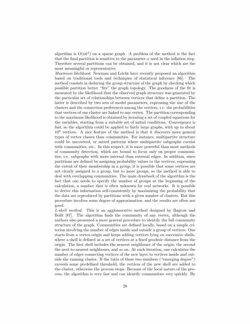
algorithm is O(nk2) on a sparse graph. A problem of the method is the factthat the final partition is sensitive to the parameter α used in the inflation step.Therefore several partitions can be obtained, and it is not clear which are themost meaningful or representative.Maximum likelihood. Newman and Leicht have recently proposed an algorithmbased on traditional tools and techniques of statistical inference [86]. Themethod consists in deducing the group structure of the graph by checking whichpossible partition better “fits” the graph topology. The goodness of the fit ismeasured by the likelihood that the observed graph structure was generated bythe particular set of relationships between vertices that define a partition. Thelatter is described by two sets of model parameters, expressing the size of theclusters and the connection preferences among the vertices, i.e. the probabilitiesthat vertices of one cluster are linked to any vertex. The partition correspondingto the maximum likelihood is obtained by iterating a set of coupled equations forthe variables, starting from a suitable set of initial conditions. Convergence isfast, so the algorithm could be applied to fairly large graphs, with up to about106 vertices. A nice feature of the method is that it discovers more generaltypes of vertex classes than communities. For instance, multipartite structurecould be uncovered, or mixed patterns where multipartite subgraphs coexistwith communities, etc.. In this respect, it is more powerful than most methodsof community detection, which are bound to focus only on proper communi-ties, i.e. subgraphs with more internal than external edges. In addition, sincepartitions are defined by assigning probability values to the vertices, expressingthe extent of their membership in a group, it is possible that some vertices arenot clearly assigned to a group, but to more groups, so the method is able todeal with overlapping communities. The main drawback of the algorithm is thefact that one needs to specify the number of groups at the beginning of thecalculation, a number that is often unknown for real networks. It is possibleto derive this information self-consistently by maximizing the probability thatthe data are reproduced by partitions with a given number of clusters. But thisprocedure involves some degree of approximation, and the results are often notgood.L-shell method. This is an agglomerative method designed by Bagrow andBollt [87]. The algorithm finds the community of any vertex, although theauthors also presented a more general procedure to identify the full communitystructure of the graph. Communities are defined locally, based on a simple cri-terion involving the number of edges inside and outside a group of vertices. Onestarts from a vertex-origin and keeps adding vertices lying on successive shells,where a shell is defined as a set of vertices at a fixed geodesic distance from theorigin. The first shell includes the nearest neighbours of the origin, the secondthe next-to-nearest neighbours, and so on. At each iteration, one calculates thenumber of edges connecting vertices of the new layer to vertices inside and out-side the running cluster. If the ratio of these two numbers (“emerging degree”)exceeds some predefined threshold, the vertices of the new shell are added tothe cluster, otherwise the process stops. Because of the local nature of the pro-cess, the algorithm is very fast and can identify communities very quickly. By

28

repeating the process starting from every vertex, one could derive a membershipmatrix M : the element Mij is one if vertex j belongs to the community of ver-tex i, otherwise it is zero. The membership matrix can be rewritten by suitablypermutating rows and columns based on their mutual distances. The distancebetween two rows (or columns) is defined as the number of entries whose el-ements differ. If the graph has a clear community structure, the membershipmatrix takes a block-diagonal form, where the blocks identify the communities.Unfortunately, the rearrangement of the matrix requires a time O(n3), so it isquite slow. In a different algorithm, local communities are discovered throughgreedy maximization of a local modularity measure [88].Algorithm of Eckmann and Moses. This is another method where communitiesare defined based on a local criterion [89]. The idea is to use the clusteringcoefficient [44] of a vertex as a quantity to distinguish tightly connected groupsof vertices. Many edges mean many loops inside a community, so the verticesof a community are likely to have a large clustering coefficient. The latter canbe related to the average distance between pairs of neighbours of the vertex.The possible values of the distance are 1 (if neighbors are connected) or 2 (ifthey are not), so the average distance lies between 1 and 2. The more trianglesthere are in the subgraph, the shorter the average distance. Since each vertexhas always distance 1 from its neighbours, the fact that the average distancebetween its neighbours is different from 1 reminds what happens when onemeasures segments on a curved surface. Endowed with a metric, representedby the geodesic distance between vertices/points, and a curvature, the graphcan be embedded in a geometric space. Communities appear as portions ofthe graph with a large curvature. The algorithm was applied to the graphrepresentation of the World Wide Web, where vertices are Web pages and edgesare the hyperlinks that take users from a page to the other. The authors foundthat communities correspond to Web pages dealing with the same topic.Algorithm of Sales-Pardo et al.. This is an algorithm designed to detect hierar-chical community structure (see Section 2.3), a realistic feature of many natural,social and technological networks, that most algorithms usually neglect. Theauthors [90] introduce first a similarity measure between pairs of vertices basedon Newman-Girvan modularity: basically the similarity between two verticesis the frequency with which they coexist in the same community in partitionscorresponding to local optima of modularity. The latter are configurations forwhich modularity is stable, i.e. it cannot increase if one shifts one vertex fromone cluster to another or by merging or splitting clusters. Next, the similaritymatrix is put in block-diagonal form, by minimizing a cost function expressingthe average distance of connected vertices from the diagonal. The blocks cor-respond to the communities and the recovered partition represents the largestscale organization level. To determine levels at lower scales, one iterates theprocedure for each subgraph identified at the previous level, which is consideredas an independent graph. The method yields then a hierarchy by construction,as communities at each level are nested within communities at higher levels.The algorithm is not fast, as both the search of local optima for modularity andthe rearrangement of the similarity matrix are performed with simulated anneal-

29

ing, but delivers good results for computer generated networks, and meaningfulpartitions for some social, technological and biological networks.Algorithm by Rosvall and Bergstrom. The modular structure can be consideredas a reduced description of a graph to approximate the whole information con-tained in its adjacency matrix. Based on this idea, Rosvall and Bergstrom [91]envisioned a communication process in which a partition of a network in com-munities represents a synthesis Y of the full structure that a signaler sends toa receiver, who tries to infer the original graph topology X from it. The bestpartition corresponds to the signal Y that contains the most information aboutX . This can be quantitatively assessed by the maximization of the mutual in-formation I(X ;Y ) [92]. The method is better than modularity optimization,especially when communities are of different size. The optimization of the mu-tual information is performed by simulated annealing, so the method is ratherslow and can be applied to graphs with up to about 104 vertices.

6 Testing Methods

When a community detection algorithm is designed, it is necessary to test itsperformance, and compare it with other methods. Ideally, one would like tohave graphs with known community structure and check whether the algorithmis able to find it, or how closely can come to it. In any case, one needs to com-pare partitions found by the method with “real” partitions. How can differentpartitions of the same graph be compared? Danon et al. [93] used a measureborrowed from information theory, the normalized mutual information. Onebuilds a confusion matrix N , whose element Nij is the number of vertices ofthe real community i that are also in the detected community j. Since thepartitions to be compared may have different numbers of clusters, N is usuallynot a square matrix. The similarity of two partitions A and B is given by thefollowing expression

I(A,B) =−2

∑cAi=1

∑cBj=1

Nij log(NijN/Ni.N.j)∑cA

i=1Ni. log(Ni./N) +

∑cBj=1

N.j log(N.j/N), (8)

where cB (cA) is the number of communities in partition A (B), Ni. is the sumof the elements of N on row i and N.j is the sum of the elements of N on columnj. Another useful measure of similarity between partitions is the Jaccard index,which is regularly used in scientometric research. Given two partitions A andB, the Jaccard index is defined as

IJ(A,B) =n11

n11 + n01 + n10

, (9)

where n11 is the number of pairs of vertices which are in the same communityin both partitions and n01 (n10) denotes the number of pairs of elements whichare put in the same community in A (B) and in different communities in B (A).A nice presentation of criteria to compare partitions can be found in Ref. [94].

30

Figure 11: Benchmark of Girvan and Newman. The three pictures correspondto zin = 15 (a), zin = 11 (b) and zin = 8 (c). In (c) the four groups arebasically invisible. Reprinted figure with permission from Guimera R, AmaralLAN, Nature 433, 895 (2005). Copyright 2005 by the Nature Publishing Group.

In the literature on community detection, algorithms have been generallytested on two types of graphs: computer generated graphs and real networks.The most famous computer generated benchmark is a class of graphs designed byGirvan and Newman [14]. Each graph consists of 128 vertices, arranged in fourgroups with 32 vertices each: 1− 32, 33− 64, 65− 96 and 97− 128. The averagedegree of each vertex is set to 16. The density of edges inside the groups istuned by a parameter zin, expressing the average number of edges shared by eachvertex of a group with the other members (internal degree). Naturally, when zinis close to 16, there is a clear community structure (see Fig. 11a), as most edgeswill join vertices of the same community, whereas when zin <= 8 there are moreedges connecting vertices of different communities and the graph looks fuzzy (seeFig. 11c). In this way, one can realize different degrees of mixing between thegroups. In this case the test consists in calculating the similarity between thepartitions determined by the method at study and the natural partition of thegraph in the four equal-sized groups. The similarity can be calculated by usingthe measure of Eq. 8, but in the literature one used a different quantity, i.e.the fraction of correctly classified vertices. A vertex is correctly classified if itis in the same cluster with at least 16 of its “natural” partners. If the modelpartition has clusters given by the merging of two or more natural groups,all vertices of the cluster are considered incorrectly classified. The number ofcorrectly classified vertices is then divided by the total size of the graph, to yielda number between 0 and 1. One usually builds many realizations of the graphfor a particular value of zin and computes the average fraction of correctlyclassified vertices, which is a measure of the sensitivity of the method. Theprocedure is then iterated for different values of zin. Many different algorithmshave been compared with each other according to the diagram where the fractionof correctly classified vertices is plotted against zin. Most algorithms usually doa good job for large zin and start to fail when zin approaches 8. The recipe tolabel vertices as correctly or incorrectly classified is somewhat arbitrary, though,and measures like those of Eqs. 8 and 9 are probably more objective. There isalso a subtle problem concerning the reliability of the test. Because of the

31

123

4 56

7

811

12

13

14

18

20

22

9

32

31

28

29

33

10

17

34

15

16

21

23

24

26

30

25

27

19

Figure 12: Zachary’s karate club network, an example of graph with knowncommunity structure. Reprinted figure with permission from Newman MEJ,Girvan M, Physical Review E 69, 026113, 2004. Copyright 2004 by the AmericalPhysical Society.

randomness involved in the process of distributing edges among the vertices,it may well be that, in specific realizations of the graph, some vertices sharemore edges with members of another group than of their own. In this case, it isinappropriate to consider the initial partition in four groups as the real partitionof the graph.

Tests on real networks usually focus on a limited number of examples, forwhich one has precise information about the vertices and their properties.

The most popular real network with a known community structure is thesocial network of Zachary’s karate club (see Fig. 12). This is a social networkrepresenting the personal relationships between members of a karate club at anAmerican university. During two years, the sociologist Wayne Zachary observedthe ties between members, both inside and outside the club [95]. At some point,a conflict arose between the club’s administrator (vertex 1) and one of the teach-ers (vertex 33), which led to the split of the club in two smaller clubs, with somemembers staying with the administrator and the others following the instruc-tor. Vertices of the two groups are highlighted by squares and circles in Fig. 12.The question is whether the actual social split could be predicted from the net-work topology. Several algorithms are actually able to identify the two classes,modulo a few intermediate vertices, which may be misclassified (e.g. vertices 3,10). Other methods are less successful: for instance, the maximum of Newman-Girvan modularity corresponds to a split of the network in four groups [53, 63].It is fundamental however to stress that the comparison of community struc-tures detected by the various methods with the split of Zachary’s karate clubis based on a very strong assumption: that the split actually reproduced theseparation of the social network in two communities. There is no real argument,beyond common wisdom, supporting this assumption.

Two other networks have frequently been used to test community detection

32

algorithms: the network of American college football teams derived by Girvanand Newman [14] and the social network of bottlenose dolphins constructed byLusseau [96]. Also for these networks the caveat applies: Nothing guaranteesthat “reasonable” communities, defined on the basis of non-topological infor-mation, must coincide with those detected by methods based only on topology.

7 The Mesoscopic Description of a Graph

Community detection algorithms have been applied to a huge variety of realsystems, including social, biological and technological networks. The partitionsfound for each system are usually similar, as the algorithms, in spite of their spe-cific implementations, are all inspired by close intuitive notions of community.What are the general properties of these partitions? The analysis of partitionsand their properties delivers a mesoscopic description of the graph, where thecommunities, and not the vertices, are the elementary units of the topology.The term mesoscopic is used because the relevant scale here lies between thescale of the vertices and that of the full graph. A simple question is whetherthe communities of a graph are usually about of the same size or whether thecommunity sizes have some special distribution. It turns out that the distri-bution of community sizes is skewed, with a tail that obeys a power law withexponents in the range between 1 and 3 [13, 22, 23, 47]. So, there seems to beno characteristic size for a community: small communities usually coexist withlarge ones. As an example, Fig. 13 shows the cumulative distribution of com-munity sizes for a recommendation network of the online vendor Amazon.com.Vertices are products and there is a connection between item A and B is B wasfrequently purchased by buyers of A. We remind that the cumulative distribu-tion is the integral of the probability distribution: if the cumulative distributionis a power law with exponent α, the probability distribution is also a power lawwith exponent α+ 1.

If communities are overlapping, one could derive a network, where the com-munities are the vertices and pairs of vertices are connected if their correspond-ing communities overlap [13]. Such networks seem to have some special proper-ties. For instance, the degree distribution is a particular function, with an initialexponential decay followed by a slower power law decay. A recent analysis hasshown that such distribution can be reproduced by assuming that the graphgrows according to a simple preferential attachment mechanism, where commu-nities with large degree have an enhanced chance to interact/overlap with newcommunities [21].

Finally, by knowing the community structure of a graph, it is possible toclassify vertices according to their roles within their community, which may al-low to infer individual properties of the vertices. A nice classification has beenproposed by Guimera and Amaral [12, 97]. The role of a vertex depends on thevalues of two indices, the z-score and the participation ratio, that determinethe position of the vertex within its own module and with respect to the othermodules. The z-score compares the internal degree of the vertex in its module

33

100

101

102

103

104

105

106

10−4

10−3

10−2

10−1

100

community size

1−cd

f, P

(k>

x)

amazon0308guide, α=−2.045

Figure 13: Cumulative distribution of community sizes for the Amazon pur-chasing network. The partition is derived by greedy modularity optimization.Reprinted figure with permission from Clauset A, Newman MEJ and Moore C,Physical Review E 70, 066111, 2004. Copyright 2004 by the Americal PhysicalSociety.

with the average internal degree of the vertices in the module. The participationratio says how the edges of the vertex are distributed among the modules. Basedon these two indices, Guimera and Amaral distinguish seven roles for a vertex.These roles seem to be correlated to functions of vertices: in metabolic net-works, for instance, vertices sharing many edges with vertices of other modules(“connectors”) are often metabolites which are more conserved across speciesthan other metabolites, i.e. they have an evolutionary advantage [12].

8 Future Directions

The problem of community detection is truly interdisciplinary. It involves sci-entists of different disciplines both in the design of algorithms and in their ap-plications. The past years have witnessed huge progresses and novelties in thistopic. Many methods have been developed, based on various principles. Theirscalability has improved by at least one power in the graph size in just a coupleof years. Currently partitions in graphs with up to millions of vertices can befound. From this point of view, the limit is close, and future improvements inthis sense are unlikely. Algorithms running in linear time are very quick, buttheir results are often not very good.

The major breakthrough introduced by the new methods is the possibilityof extracting graph partitions with no preliminary knowledge or inputs about

34

the community structure of the graph. Most new algorithms do not need toknow how many communities there are, a major drawback of computer scienceapproaches: they derive this information from the graph topology itself. Sim-ilarly, algorithms of new generation are able to select one or a few meaningfulpartitions, whereas social science approaches usually produce a whole hierar-chy of partitions, which they are unable to discriminate. Especially in the lasttwo years, the quality of the output produced by some algorithms has consider-ably improved. Realistic aspects of community structure, like overlapping andhierarchical communities, are now often taken into account.

The main question is: is there at present a good method to detect commu-nities in graphs? The answer depends on what is meant by “good”. Severalalgorithms give satisfactory results when they are tested as described in Sec-tion 6: in this respect, they can be considered good. However, if examined inmore detail, some methods disclose serious limits and biases. For instance, themost popular method used nowadays, modularity optimization, is likely to giveproblems in the analysis of large graphs. Most algorithms are likely to fail insome limit, still one can derive useful indications from them: from the compar-ison of partitions derived by different methods one could extract the cores ofreal communities. The ideal method is one that delivers meaningful partitionsand handles overlapping communities and hierarchy, possibly in a short time.No such method exists yet.

Finding a good method for community detection is a crucial endeavour inbiology, sociology and computer science. In particular, biologists often relyon the application of clustering techniques to classify their data. Due to thebioinformatics revolution, gene regulatory networks, protein-protein interactionnetworks, metabolic networks, etc., are now much better known that they usedto be in the past and finally susceptible to solid quantitative investigations.Uncovering their modular structure is an open challenge and a necessary stepto discover properties of elementary biological constituents and to understandhow biological systems work.

References

[1] Euler L (1736) Solutio problematis ad geometriam situs pertinentis. Com-mentarii Academiae Petropolitanae, Vol 8, pp 128-140

[2] Bollobas B (1998) Modern Graph Theory. Springer Verlag, New York (USA).

[3] Wasserman S, Faust K (1994) Social Network Analysis: Methods and Ap-plications. Cambridge University Press, Cambridge (UK).

[4] Scott JP (2000) Social Network Analysis. Sage Publications Ltd., London(UK).

[5] Barabasi Al, Albert R (2002) Statistical mechanics of complex networks.Reviews of Modern Physics, Vol 74, pp 47–97

35

[6] Dorogovtsev SN, Mendes JFF (2003) Evolution of Networks: from biologicalnets to the Internet and WWW. Oxford University Press, Oxford (UK)

[7] Newman MEJ (2003) The structure and function of complex networks. SIAMReview, Vol 45, pp 167–256

[8] Pastor-Satorras R, Vespignani A (2004) Evolution and structure of the Inter-net: A statistical physics approach. Cambridge University Press, Cambridge(UK)

[9] Boccaletti S, Latora V, Moreno Y, Chavez M, Hwang DU (2006) ComplexNetworks: Structure and Dynamics. Physics Reports, Vol 424, pp 175–308

[10] Erdos P, Renyi A (1959) On Random Graphs. Publicationes MathematicaeDebrecen, Vol 6, pp 290–297

[11] Flake GW, Lawrence S, Lee Giles C, Coetzee FM (2002) Self-Organizationand Identification of Web Communities. IEEE Computer, Vol 35, No 3, pp66–71

[12] Guimera R, Amaral LAN (2005) Functional cartography of complexmetabolic networks. Nature 433, pp 895-900

[13] Palla G, Derenyi I, Farkas I, Vicsek T (2005) Uncovering the overlappingcommunity structure of complex networks in nature and society. Nature, Vol435, pp 814-818

[14] Girvan M, Newman MEJ (2002) Community structure in social and biolog-ical networks. Proceedings of the National Academy of Science of the USA,Vol 99, No 12, pp 7821–7826

[15] Lusseau D, Newman MEJ (2004) Identifying the role that animals play intheir social networks. Proceedings of the Royal Society of London B, Vol271, pp S477–S481

[16] Pimm SL (1979) The structure of food webs. Theoretical Population Bi-olology, Vol 16, pp 144–158

[17] Krause AE, Frank KA, Mason DM, Ulanowicz RE, Taylor WW (2003)Compartments exposed in food-web structure. Nature, Vol 426, p 282–285

[18] Granovetter M (1973) The Strength of Weak Ties. American Journal ofSociology, Vol 78, pp 1360–1380

[19] Burt RS (1976) Positions in Networks. Social Forces, Vol 55, No 1, pp93-122

[20] Freeman LC (1977) A Set of Measures of Centrality Based on Betweenness.Sociometry, Vol 40, No 1, pp 35–41

36

[21] Pollner P, Palla G, Vicsek T (2006) Preferential attachment of communities:The same principle, but a higher level. Europhysics Letters, Vol 73, No 3,pp 478–484

[22] Newman MEJ (2004) Detecting community structure in networks. Euro-pean Physical Journal B, Vol 38, pp 321–330

[23] Danon L, Duch J, Arenas A, Dıaz-Guilera A (2007) Community structureidentification. Large Scale Structure and Dynamics of Complex Networks:From Information Technology to Finance and Natural Science, Caldarelli Gand Vespignani A, Eds., World Scientific, Singapore, pp 93–114

[24] Bron C, Kerbosch J (1973) Finding all cliques on an undirected graph.Communications of ACM, Vol 16, pp 575–577

[25] Radicchi F, Castellano C, Cecconi F, Loreto V, Parisi D (2004) Defining andidentifying communities in networks. Proceedings of the National Academyof Science of the USA, Vol 101, No 9, pp 2658–2663

[26] Newman MEJ, Girvan M (2004) Finding and evaluating community struc-ture in networks. Physical Review E, Vol 69, 026113

[27] Arenas A, Fernandez A, Fortunato S, Gomez S (2007) Motif-based com-munities in complex networks. Eprint arXiv:0710.0059 in www.arxiv.org

[28] Reichardt J, Bornholdt S (2006) Statistical mechanics of community detec-tion. Physical Review E, Vol 74, 016110

[29] Massen CP, Doye JPK (2006) Thermodynamics of community structure.Eprint cond-mat/0610077 in www.arxiv.org

[30] Arenas A, Duch J, Fernandes A, Gomez S (2007) Size reduction of complexnetworks preserving modularity. New Journal of Physics, Vol 9, No 6, pp176–180

[31] Guimera R, Sales-Pardo M, Amaral LAN (2004) Modularity from fluctua-tions in random graphs and complex networks. Physical Review E, Vol 70,025101(R)

[32] Fortunato S, Barthelemy M (2007) Resolution limit in community detec-tion. Proceedings of the National Academy of Science of the USA, Vol 104,No 1, pp 36–41

[33] Gfeller D, Chappelier J-C, De Los Rios P (2005) Finding instabilities inthe community structure of complex networks. Physical Review E, Vol 72,056135

[34] Pothen A (1997) Graph partitioning algorithms with applications to scien-tific computing. In Parallel Numerical Algorithms, Keyes DE, Sameh A andVenkatakrishnan V, Eds., Kluwer Academic Press, pp 323–368

37

http://arxiv.org/abs/0710.0059

http://arxiv.org/abs/cond-mat/0610077

[35] Kernighan BW, Lin S (1970) An efficient heuristic procedure for partition-ing graphs. The Bell System Technical Journal, Vol 49, pp 291–307

[36] Golub GH, Van Loan CF (1989) Matrix computations. John Hopkins Uni-versity Press, Baltimore, MD, USA

[37] J. B. MacQueen (1967) Some methods for classification and analysis of mul-tivariate observations. Proceedings of 5-th Berkeley Symposium on Mathe-matical Statistics and Probability, Berkeley, University of California Press,pp 281-297

[38] Brandes, U (2001) A faster algorithm for betweenness centrality. Journalof Mathematical Sociology, Vol 25, No 2, pp 163–177

[39] Newman MEJ (2005) A measure of betweenness centrality based on randomwalks. Social Networks, Vol 27, pp 39–54

[40] Tyler JR, Wilkinson DM, Huberman BA (2003) Email as spectroscopy:automated discovery of community structure within organizations. Proceed-ing of the First International Conference on Communities and Technologies,Huysman M, Wenger E and Wulf V, Eds., Kluwer Academic Press, Amster-dam.

[41] Wilkinson DM, Huberman BA (2004) A method for finding communities ofrelated genes. Proceedings of the National Academy of Science of the USA,Vol 101, Suppl 1, pp 5241–5248

[42] Latora V, Marchiori M (2001) Efficient behavior of small-world networks.Physical Review Letters, Vol 87, 198701

[43] Fortunato S, Latora V, Marchiori M (2004) A method to find commu-nity structures based on information centrality. Physical Review E, Vol 70,056104

[44] Watts D, Strogatz SH (1998) Collective dynamics of “small-world” net-works. Nature, Vol 393, pp 440–442

[45] Brandes U, Delling D, Gaertler M, Gorke R, Hoefer M, Nikoloski Z, WagnerD (2007) On finding graph clusterings with maximum modularity. Proceed-ings of the 33rd International Workshop on Graph-Theoretical Concepts inComputer Science (WG’07), Springer Verlag, Berlin-Heidelberg, Germany.

[46] Newman MEJ (2004) Fast algorithm for detecting community structure innetworks. Physical Review E, Vol 69, 066133

[47] Clauset A, Newman MEJ, Moore C (2004) Finding community structurein very large networks. Physical Review E, Vol 70, 066111

[48] Danon L, Dıaz-Guilera A, Arenas A (2006) The effect of size heterogene-ity on community identification in complex networks. Journal of StatisticalMechanics: Theory and Experiment, Issue 11, P11010

38

[49] Pujol JM, Bejar J, Delgado J (2006) Clustering algorithm for determiningcommunity structure in large networks. Physical Review E, Vol 74, 016107

[50] Kirkpatrick S, Gelatt CD, Vecchi MP (1983) Optimization by simulatedannealing. Science, Vol 220, No 4598, pp 671–680

[51] Massen CP, Doye JPK (2005) Identifying communities within energy land-scapes. Physical Review E, Vol 71, 046101

[52] Boettcher S, Percus AG (2001) Optimization with extremal dynamics.Physical Review Letters, Vol 86, pp 5211–5214

[53] Duch J, Arenas A (2005) Community detection in complex networks usingextremal optimization. Physical Review E, Vol 72, 027104

[54] Newman MEJ (2006) Modularity and community structure in networks.Proceedings of the National Academy of Science of the USA, Vol 103, No.23, pp 8577–8582

[55] Newman MEJ (2006) Finding community structure in networks using theeigenvectors of matrices. Physical Review E, Vol 74, 036104

[56] Reichardt J, Bornholdt S (2007) Partitioning and modularity of graphswith arbitrary degree distribution. Physical Review E, Vol 76, 015102(R)

[57] Reichardt J, Bornholdt S (2006) When are networks truly modular? Phys-ica D, Vol 224, pp 20–26

[58] Kumpula JM, Saramaki J, Kaski K, Kertesz J (2007) Limited resolutionin complex network community detection with Potts model approach. Eu-ropean Physical Journal B, Vol 56, pp 41–45

[59] Arenas A, Fernandes A, Gomez S (2007) Multiple resolution of the modularstructure of complex networks. Eprint physics/0703218 at www.arxiv.org

[60] Ruan J, Zhang W (2007) Identifying network communities with high res-olution. Eprint arXiv: 0704.3759 in www.arxiv.org, to appear in PhysicalReview E

[61] Kumpula JM, Saramaki J, Kaski K, Kertesz J (2007) Limited resolu-tion and multiresolution methods in complex network community detection.Noise and Stochastics in Complex Systems and Finance, Kertesz J, Born-holdt S and Mantegna RN, Eds. Proceedings of the SPIE, Vol 6601, pp660116

[62] Muff S, Rao F, Caflisch A (2005) Local modularity measure for networkclusterizations. Physical Review E, Vol 72, 056107

[63] Donetti L, Munoz MA (2004) Detecting network communities: a new sys-tematic and efficient algorithm. Journal of Statistical Mechanics: Theoryand Experiment, P10012

39

http://arxiv.org/abs/physics/0703218

[64] Capocci A, Servedio VDP, Caldarelli G, Colaiori F (2004) Detecting com-munities in large networks. Physica A, Vol 352, No 2-4, pp 669-676

[65] Wu F, Huberman BA (2004) Finding communities in linear time: a physicsapproach. European Physical Journal B, Vol 38, pp 331-338

[66] Eriksen KA, Simonsen I, Maslov S, Sneppen K (2003) Modularity andextreme edges of the Internet. Physical Review Letters, Vol 90, No 14, 148701

[67] Simonsen I, Eriksen KA, Maslov S, Sneppen K (2004) Diffusion on complexnetworks: a way to probe their large-scale topological structure. Physica A,Vol 336, pp 163–173

[68] Wu FY (1982) The Potts model. Reviews of Modern Physics, Vol 54, pp235–268

[69] Blatt M, Wiseman S, Domany E (1996) Superparamagnetic clustering ofdata. Physical Review Letters, Vol 76, No 18, pp 3251–3254

[70] Reichardt J, Bornholdt S (2004) Detecting fuzzy community structure incomplex networks. Physical Review Letters, Vol 93, No 21, 218701

[71] Reichardt J, Bornholdt S (2006) Statistical mechanics of community detec-tion Physical Review E, Vol 74, 016110

[72] Mezard M, Parisi G, Virasoro M (1987) Spin glass theory and beyond.World Scientific Publishing Company, Singapore.

[73] Zhou H (2003) Network landscape from a Brownian particle’s perspective.Physical Review E, Vol 67, 041908

[74] Zhou H (2003) Distance, dissimilarity index, and network community struc-ture. Physical Review E, Vol 67, 061901

[75] Zhou H, Lipowsky R (2004) Network Brownian motion: A new method tomeasure vertex-vertex proximity and to identify communities and subcom-munities. Lecture Notes in Computer Science, Vol 3038, pp 1062–1069

[76] Latapy M, Pons P 92005) Computing communities in large networks usingrandom walks. Lecture Notes in Computer Science, Vol 3733, pp 284–293

[77] Arenas A, Dıaz-Guilera A, Perez-Vicente CJ (2006) Synchronization revealstopological scales in complex networks. Physical Review Letters, Vol 96,114102

[78] Kuramoto Y (1984) Chemical Oscillations, Waves and Turbulence.Springer-Verlag, Berlin, Germany

[79] Arenas A, Dıaz-Guilera A (2007) Synchronization and modularity in com-plex networks. European Physical Journal ST, Vol 143, pp 19–25

40

[80] Boccaletti S, Ivanchenko M, Latora V, Pluchino A, Rapisarda A (2007)Detecting complex network modularity by dynamical clustering. PhysicaReview E, Vol 76, 045102(R)

[81] Pluchino A, Latora V, Rapisarda A (2005) Changing opinions in a changingworld: a new perspective in sociophysics. International Journal of ModernPhysics C, Vol 16, No 4, pp 505–522

[82] Farkas I, bel D, Palla G, Vicsek T (2007) Weighted network modules. NewJournal of Physics, Vol 9, pp 180

[83] Palla G, Farkas IJ, Pollner P, Derenyi I, Vicsek T (2007) Directed networkmodules. New Journal of Physics, Vol 9, pp 186

[84] Palla G, Barabasi A-L, Vicsek T (2007) Quantifying social groups evolution.Nature, Vol 446, pp 664–667

[85] van Dongen S (2000) Graph Clustering by Flow Simulation. PhD thesis,University of Utrecht, Netherlands

[86] Newman MEJ, Leicht E (2007) Mixture models and exploratory analysisin networks. Proceedings of the National Academy of Science of the USA,Vol 104, No 23, pp 9564–9569

[87] Bagrow JP, Bollt EM (2005) Local method for detecting communities.Physical Review E, Vol 72, 046108

[88] Clauset A (2005) Finding local community structure in networks. PhysicalReview E, Vol 72, 026132

[89] Eckmann J.-P, Moses E (2002) Curvature of co-links uncovers hidden the-matic layers in the World Wide Web. Proceedings of the National Academyof Science of the USA, Vol 99, No 9, pp 5825–5829

[90] Sales-PardoM, Guimera R, Amaral LAN (2007) Extracting the hierarchicalorganization of complex systems. Eprint arXiv:0705.1679 in www.arxiv.org

[91] Rosvall M, Bergstrom CT (2007) An information-theoretic framework forresolving community structure in complex networks. Proceedings of the Na-tional Academy of Science of the USA, Vol 104, No 18, pp 7327–7331

[92] Shannon CE, Weaver V (1949) The Mathematical Theory of Communica-tion. University of Illinois Press, Champaign, USA

[93] Danon L, Dıaz-Guilera A, Duch J, Arenas A (2005) Comparing commu-nity structure identification. Journal of Statistical Mechanics: Theory andExperiment, P09008

[94] Gustafsson M, Hornquist M, Lombardi A (2006) Comparison and validationof community structures in complex networks. Physica A, Vol 367, pp 559–576

41

http://arxiv.org/abs/0705.1679

[95] Zachary WW (1977) An information flow model for conflict and fission insmall groups. Journal of Anthropological Research, Vol 33, pp 452–473

[96] Lusseau D (2003) The emergent properties of a dolphin social network.Proceedings of the Royal Society of London B, Vol 270 (Suppl. 2), pp S186–188

[97] Guimera R, Amaral LAN (2005) Cartography of complex networks: mod-ules and universal roles. Journal of Statistical Mechanics: Theory and Ex-periment, P02001

42

Documents

Community Structure in Graphs - arXiv · Section 2 is about the basic elements of community detection, starting from the deﬁnition of community. The classical problem of graph partitioning