COMMUNITY INTERACTIONS AND ENVIRONMENTAL DRIVERS OF

HOST-PARASITE DYNAMICS IN AN ESTUARINE SYSTEM

by

ALYSSA-LOIS MADDEN GEHMAN

(Under the Direction of James E. Byers)

ABSTRACT

Not all hosts, communities or environments are equally hospitable for parasites.

Direct and indirect interactions between parasites and their predators, competitors and the

environment can influence variability in host exposure, susceptibility and subsequent

infection, and these influences may vary across spatial scales. I evaluate abiotic and

biotic drivers of parasite abundance and host-parasite dynamics utilizing the parasite

Loxothylacus panopaei, which infects an oyster reef dwelling mud crab Eurypanopeus

depressus. I conducted a survey of host, parasite, and predator abundance, parasite

prevalence, and environmental characteristics of oyster reef communities from Florida to

North Carolina. I found that water depth, predators and host characteristics were all

positively correlated with the probability of infection within a reef. I further investigated

whether the predatory crab Callinectes sapidus and other predators preferentially feed on

E. depressus infected with L. panopaei and evaluated a mechanism behind prey choice. I

evaluated prey choice through mesocoms experiments, field tethering experiments and

behavioral trials. I found that C. sapidus preferentially consumed infected E. depressus

in the lab and this pattern was confirmed in the field. Contrary to expectations, I found

that infected crabs ran faster in behavioral trials than uninfected E. depressus. Finally, I

evaluated the influence of temperature on host and parasite survival and parasite

reproduction. I quantified thermal response curves encompassing the thermal breadth of

both host and parasite, and found a thermal mismatch in survival optima between infected

and uninfected hosts. I then parameterized a physiologically based epidemiological

model to predict the sensitivity of a host-parasite system to seasonal varying temperature

and future climate change scenarios. I found that the model accurately recreates annual

cycles and seasonality in this host-parasite system, and that the parasite is locally

extirpated from the system under a 3ºC warming scenario. Together, these findings

demonstrate the importance of community interactions and environmental drivers in

driving the abundance and prevalence of L. panopaei infection in E. depressus at a

regional, local scale and under climate warming scenarios.

INDEX WORDS: Disease Ecology, Marine Invertebrates, Host-Parasite Interactions,

Predation, Climate Change, Rhizocephalans, Loxothylacus

panopaei, Eurypanopeus depressus

COMMUNITY INTERACTIONS AND ENVIRONMENTAL DRIVERS OF

HOST-PARASITE DYNAMICS IN AN ESTUARINE SYSTEM

by

ALYSSA-LOIS MADDEN GEHMAN

B.A. Colorado College, 2005

M.S. Western Washington University, 2008

A Dissertation Submitted to the Graduate Faculty of The University of Georgia in Partial

Fulfillment of the Requirements for the Degree

DOCTOR OF PHILOSOPHY

ATHENS, GA

2016

© 2016

ALYSSA-LOIS MADDEN GEHMAN

All Rights Reserved

COMMUNITY INTERACTIONS AND ENVIRONMENTAL DRIVERS OF

HOST-PARASITE DYNAMICS IN AN ESTUARINE SYSTEM

by

ALYSSA-LOIS MADDEN GEHMAN

Major Professor: James E. Byers

Committee: Vanessa Ezenwa Sonia Altizer Jim Porter Bill Fitt

Electronic Version Approved:

Suzanne Barbour Dean of the Graduate School The University of Georgia May 2016

iv

DEDICATION

I dedicate this dissertation to my grandparents:

Stephen and Lois Madden

and

Helen and Earl Gehman

Your hard work, dedication, joy and care for the world and the people in it

remain an inspiration.

v

ACKNOWLEDGEMENTS

I would like to thank my advisor Jeb Byers for permanently changing my

vocabulary about science by breaking down the PhD process into a select few idioms.

Thank you, Jeb, for helping me to develop a dissertation that puts a fire in my belly, for

always reminding me when I’m putting the cart before the horse and for poking holes in

every idea I’ve ever had to make sure they still float. Thank you for helping me to find

the low hanging fruit in my system, and for red-flagging any issues with my big picture,

which I was always seemed to be chasing down. I hope to be able to take these lessons

forward and do cutting edge science that is always the biggest bang for my buck.

Thank you to my committee, Sonia Altizer, Vanessa Ezenwa, Jim Porter and Bill

Fitt, who have provided amazing feedback, support and critically important criticism

throughout this process. Thanks to Richard Hall for showing me how to using the

ecological knowledge of my system to develop a epidemiological model. Thank you to

the remarkably supportive Odum School of Ecology faculty, who provided both

encouragement and feedback in the hallway, at potlucks, in meetings, at GSS and at first

Friday. In particular, Craig Osenberg, Alan Covich, Ford Ballantyne, Andrew Park,

Laurie Fowler, Courtney Murdock, Cathy Pringle, J.P. Schmidt, Patrick Stephens, John

Wares, Seth Wegner, Bernie Patten, Bud Freeman, Mary Freeman and Ron Carrol.

Thank you to the OSE staff who regularly go above and beyond to support my work,

including Beth Gavrilles, Brian Perkins, Emily Schattler, Katherine Adams, Elaine

vi

Dunbar, Tyler Ingram, Brenda Mattox, Lee Snelling and Shialoh Wilson. Thank you to

the Computational Ecology and Epidemiology Study Group for insights gained after

spending several hours sitting with my research questions.

I am incredibly grateful for the graduate community here at the Odum School that

creates and trains an amazing group of collaborators and friends. I was lucky enough to

have a group of co-mentors, the Parasite Ladies, who were willing to talk about parasites,

read about parasites, write about parasites, dream about parasites…and through that

connection mentor each other through all our trials and tribulations of graduate school in

such a fun way. Thank you to Carrie Keough, Dara Satterfield, Sarah Budischak and

Alexa McKay. Under the direction of Jeb, the Byers lab collaborated like it was our job

(oh wait…). I am so grateful for the hours of feedback on ideas, papers, proposals, help

in the field and general silliness to keep us all sane. Thanks to Virginia Schutte, Bill

McDowell, Jean Lee, Rachel Smith, Linsey Harram, Carrie Keough, Daniel Harris, Safra

Altman, Jenna Malek, Heidi Weiskel, Caitlin Yaeger, Kaitlin Kinney, Paula Pappalardo

and Jeff Beauvais. In addition, we gained the Osenberg lab in our last few years, who

have provided valuable insight on my work. Thanks to Anya Brown, Elizabeth Hamman,

Rebecca Atkins, Amy Briggs and Greg Jacobs. Thanks to the OSE community of folks

who are willing to talk science with me and read drafts of papers, including Carly

Phillips, Chao Song, Tad Dallas, Dan Becker, Kyle McKay, Troy Simon, Ross Pringle,

Cecilia Sanchez and Reni Kaul.

My research was made possible by a team of excellent undergraduates that helped

conduct my field and lab work. In particular, thanks to Aaron Penn for the weeks/months

of his life spent sorting through oysters for crabs and filtering and changing seawater.

vii

Thanks also to Sarah Perry, Rachel Usher, Zack Holmes, Amanda Calfee, Morgan

Walker, Stuart Sims, Morgan Mahaffey, Gabriel Mills, Katie Shaw, Stephanie Shaw, Tim

Montgomery, Allison Capper, Michael Holden, and Kaleigh Davis.

I had the pleasure of being a Wormsloe Institute for Environmental History

Fellow during my time here at UGA. Thank you to Craig and Diana Barrow for the

generosity and hospitality in sharing their amazing property with us, and for supporting

such a range of research fellows. I count myself as incredibly lucky to have been able to

spend so much time living in the forest near the marsh. Thanks to Sarah Ross for her

support of my research and for the outreach and career training opportunities she

provided me through this fellowship. Thanks to the Wormsloe fellows and faculty for

their insights and collaboration over the years, including Paul Cady, Holly Campbell,

Ania Majewska, Nancy O’Hare, Allesandro Pasqua, Emily Cornelius, Marguerite

Madden, Tommy Jordan, Andy Davis, Sonia Altizer, Ron Carrol and Cari Goetcheus.

The much of my research was conducted at the Skidaway Institute for

Oceanography. Thanks to the faculty and staff of SKIO for all their support, from

keeping our seawater system and air conditioners running, to lending chillers and freezer

space. Particular thanks to Larsen Moore, Harry Carter, Neil Mizel, Clark Alexander, Zac

Tait, Tina Walters, Bob Allen, Dee King, Lisa Doser, Chuck Hartman, Bill Savidge and

Catherine Edwards. Thank you to UGA MAREX, and Tom Bliss for providing me with

lab space. I also conducted some research on Sapelo Island, and would like to thank the

faculty and staff of the University of Georgia Marine Institute, including Merryl Albers,

Jacob Shalack, Caroline Reddy, Mary Price, Gracie Townsend and Barbara Price.

viii

I am lucky enough to have a huge community of support outside of UGA as well,

who have encouraged me, entertained me, read my papers and discussed my research

ideas with me over beers. Thank you to Melinda Simmons and her whole family for

regularly welcoming me into the fold, spoiling me rotten and generally providing a

wonderful, happy, retreat for me to return to. Thank you to my Savannah support group,

including Ellie Covington, Safra Altman, Ann and Andrew Hartzel, Jamie Smith Arkins,

Olivia McIntosh, Ashby Nix Worley, Brian Corely, Andrew Patterson and Shelly

Kreuger. Thank you to my acroyoga community for keeping me sane, especially Juli

Bierworth, Willow Tracy and Dave Frank. Thank you to my first, extended, pre-PhD

cohort, Judit Pungor, Megan Jensen, Alison Haupt, Rachael Bay, Chelsea Wood, Malin

Pinsky, Kristin Hunter-Thomas, Mike Vardaro, Kevin Miklasz, Nishad Jayasundara,

Malithi De Silva, Julie Stewart Lowndes, Kenan Matterson, Ashley Booth, Luke Miller,

Sarah Tepler Drobnitch, and Michelle Ow, for supporting me through applying to this

program, and then from afar and across many life stages continuing to support me, enjoy

the world with me and encourage me. Thank you to Amanda Winans, Jalena Bown and

Amber Mitrotti for continuing to make me laugh through our many different life stages.

I am grateful to the amazing mentors and educators who showed me the mysteries

and beauty of science and encouraged me to follow my dreams. Thank you to Johannes

Steegmans, who sparked my interest in science, and insisted that I was good at math.

Thank you to Paul Spangenburg, Jonathan Stever, Tom Hudson and Craig MacGowan at

Garfield High School, who introduced me to the ocean and field research. Thanks to Ron

Hathaway at Colorado College, who showed me how fascinating parasites can be. Thanks

to Cathy Pfister, Tim Wootton, Kathy Van Alstyne, Mark Denny, George Somero, Steve

ix

Palumbi, Erin Grey, Ole Shelton, Julie Collens and Bob Paine who introduced me to an

incredible array of ways to study ecology in the field. Thanks to Brian Bingham, who

prepared me so well for my science career.

Finally, I need to thank my family for all their support throughout out my

education. Edan, you are an inspiration and a joy. You’ve helped me in the lab, edited

my grammar, endured the southeastern bugs, taken me skiing, provided me with a

legitimate connection for elementary school science outreach and can make me laugh

harder than anyone else in the world. Mom, when it came to my education and career the

question was never “if’ but “how” we were going to make it happen…starting with the

remarkably prescient fight with the Seattle School placement folks to get me to Garfield

and continuing in so many fabulous and silly ways since. You’ve read science papers,

you’ve edited scripts for my crowd-funding campaign, and you’ve even come to the lab

and taken down data and changed water in my crab condos. I look forward to our future

collaborations, exploring the interplay between science, art and performance. Dad, I am

so grateful for the undying curiosity about how the world works that you inspired in me

from the beginning. I love watching you ‘out-curious’ three year olds, knowing that

you’re continuing to inspire an appreciation for pattern, beauty and science. I’ve love our

joint discoveries of where the fields of defibrillator algorithms and marine disease

ecology overlap, and that even in graduate school you can still help me with my math

(I’m much more calm now then I was in middle school I believe). Maybe someday we

can make a heart monitor for a marine invert together.

x

TABLE OF CONTENTS

Page

DEDICATION……………………………………………………………………………iv

ACKNOWLEDGEMENTS……………………………………………………………….v

CHAPTER

1 INTRODUCTION AND LITERATURE REVIEW……………………...1

Literature cited…………………………………………………………....5

2 PREDATORS, ENVIRONMENT AND HOST CHARACTERISTICS

INFLUENCE THE PROBABILITY OF INFECTION BY AN INVASIVE

PARASITE……………………………………………………………….9

Abstract…………………………………………………………………..10

Introduction……………………………………………………………....10

Materials and Methods…………………………………………………...13

Results…………………………………………………………………....18

Discussion………………………………………………………………..20

Literature cited…………………………………………………………...24

3 NON-NATIVE PARASITE ENHANCES SUSCEPTIBILITY OF HOST

TO NATIVE

PREDATORS………………………………………………...................39

Summary………………………………………………………..……….40

xi

Introduction……………………………………………………………...41

Materials and Methods…………………………………………………..44

Results…………………………………………………………………...48

Discussion……………………………………………………………….49

Literature cited…………………………………………………………..52

4 INCREASED TEMPERATURES DIFFERENTIALLY IMPACT

PARASITES, FREEING HOST FROM

INFECTION……………………………….............................................65

Abstract………………………………………………………………….66

Introduction, Results and Discussion.…………………………………...66

Supporting Materials……...……………………………………………..78

Literature cited……………………………………………………..…...103

5 CONCLUSION…………………………………………………………110

Literature cited………………………………………………………….112

1

CHAPTER 1

INTRODUCTION

Sensitive to heat

Native predator consumes

New climate may kill

Parasites exist within free-living organisms in our ecosystems, and by some

estimates there are as many as four parasites per free-living host (Windsor 1998).

Regardless of their exact relative abundance, parasites are increasingly recognized as

influential members of ecological communities, contributing to community interactions

and biodiversity (Wood and Johnson 2015). Parasite have a negative direct effect on

their hosts by definition, and at the population level some parasite are able to regulate

host dynamics (Dobson and Hudson 1992). At the community level, parasites can alter

community composition through alteration of host feeding rates (Wood et al. 2007). At

the ecosystem level parasite add to the complexity of foodwebs (Hechinger et al. 2011),

and can make up a substantial proportion of the biomass within an ecosystem (Kuris et al.

2008).

While most free-living species are associated with at least one parasite, not all

individuals within a species, or habitats within the species range will have parasites. As

2

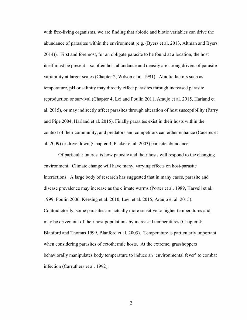
with free-living organisms, we are finding that abiotic and biotic variables can drive the

abundance of parasites within the environment (e.g. (Byers et al. 2013, Altman and Byers

2014)). First and foremost, for an obligate parasite to be found at a location, the host

itself must be present – so often host abundance and density are strong drivers of parasite

variability at larger scales (Chapter 2; Wilson et al. 1991). Abiotic factors such as

temperature, pH or salinity may directly effect parasites through increased parasite

reproduction or survival (Chapter 4; Lei and Poulin 2011, Araujo et al. 2015, Harland et

al. 2015), or may indirectly affect parasites through alteration of host susceptibility (Parry

and Pipe 2004, Harland et al. 2015). Finally parasites exist in their hosts within the

context of their community, and predators and competitors can either enhance (Cáceres et

al. 2009) or drive down (Chapter 3; Packer et al. 2003) parasite abundance.

Of particular interest is how parasite and their hosts will respond to the changing

environment. Climate change will have many, varying effects on host-parasite

interactions. A large body of research has suggested that in many cases, parasite and

disease prevalence may increase as the climate warms (Porter et al. 1989, Harvell et al.

1999, Poulin 2006, Keesing et al. 2010, Levi et al. 2015, Araujo et al. 2015).

Contradictorily, some parasites are actually more sensitive to higher temperatures and

may be driven out of their host populations by increased temperatures (Chapter 4;

Blanford and Thomas 1999, Blanford et al. 2003). Temperature is particularly important

when considering parasites of ectothermic hosts. At the extreme, grasshoppers

behaviorally manipulates body temperature to induce an ‘environmental fever’ to combat

infection (Carruthers et al. 1992).

3

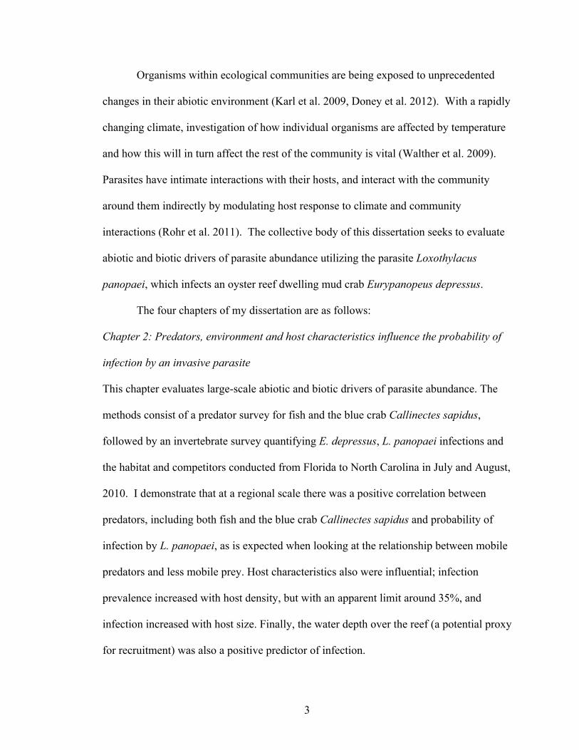
Organisms within ecological communities are being exposed to unprecedented

changes in their abiotic environment (Karl et al. 2009, Doney et al. 2012). With a rapidly

changing climate, investigation of how individual organisms are affected by temperature

and how this will in turn affect the rest of the community is vital (Walther et al. 2009).

Parasites have intimate interactions with their hosts, and interact with the community

around them indirectly by modulating host response to climate and community

interactions (Rohr et al. 2011). The collective body of this dissertation seeks to evaluate

abiotic and biotic drivers of parasite abundance utilizing the parasite Loxothylacus

panopaei, which infects an oyster reef dwelling mud crab Eurypanopeus depressus.

The four chapters of my dissertation are as follows:

Chapter 2: Predators, environment and host characteristics influence the probability of

infection by an invasive parasite

This chapter evaluates large-scale abiotic and biotic drivers of parasite abundance. The

methods consist of a predator survey for fish and the blue crab Callinectes sapidus,

followed by an invertebrate survey quantifying E. depressus, L. panopaei infections and

the habitat and competitors conducted from Florida to North Carolina in July and August,

2010. I demonstrate that at a regional scale there was a positive correlation between

predators, including both fish and the blue crab Callinectes sapidus and probability of

infection by L. panopaei, as is expected when looking at the relationship between mobile

predators and less mobile prey. Host characteristics also were influential; infection

prevalence increased with host density, but with an apparent limit around 35%, and

infection increased with host size. Finally, the water depth over the reef (a potential proxy

for recruitment) was also a positive predictor of infection.

4

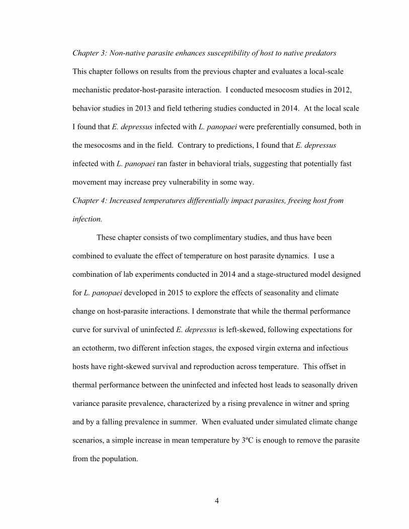
Chapter 3: Non-native parasite enhances susceptibility of host to native predators

This chapter follows on results from the previous chapter and evaluates a local-scale

mechanistic predator-host-parasite interaction. I conducted mesocosm studies in 2012,

behavior studies in 2013 and field tethering studies conducted in 2014. At the local scale

I found that E. depressus infected with L. panopaei were preferentially consumed, both in

the mesocosms and in the field. Contrary to predictions, I found that E. depressus

infected with L. panopaei ran faster in behavioral trials, suggesting that potentially fast

movement may increase prey vulnerability in some way.

Chapter 4: Increased temperatures differentially impact parasites, freeing host from

infection.

These chapter consists of two complimentary studies, and thus have been

combined to evaluate the effect of temperature on host parasite dynamics. I use a

combination of lab experiments conducted in 2014 and a stage-structured model designed

for L. panopaei developed in 2015 to explore the effects of seasonality and climate

change on host-parasite interactions. I demonstrate that while the thermal performance

curve for survival of uninfected E. depressus is left-skewed, following expectations for

an ectotherm, two different infection stages, the exposed virgin externa and infectious

hosts have right-skewed survival and reproduction across temperature. This offset in

thermal performance between the uninfected and infected host leads to seasonally driven

variance parasite prevalence, characterized by a rising prevalence in witner and spring

and by a falling prevalence in summer. When evaluated under simulated climate change

scenarios, a simple increase in mean temperature by 3ºC is enough to remove the parasite

from the population.

5

In sum, this dissertation demonstrates the importance of community interactions

and environmental drivers in driving the abundance of L. panopaei infection in E.

depressus at both a regional and local scale.

Literature Cited

Altman, I., and J. E. Byers. 2014. Large-scale spatial variation in parasite communities

influenced by anthropogenic factors. Ecology.

Araujo, R. V., M. R. Albertini, A. L. Costa-da-Silva, L. Suesdek, N. C. S. Franceschi, N.

M. Bastos, G. Katz, V. A. Cardoso, B. C. Castro, M. L. Capurro, and V. L. A. C.

Allegro. 2015. São Paulo urban heat islands have a higher incidence of dengue than

other urban areas. Brazilian Journal of Infectious Diseases 19:146–155.

Blanford, S., and M. B. Thomas. 1999. Host thermal biology: the key to understanding

host–pathogen interactions and microbial pest control? Agricultural and Forest

Entomology 1:195–202.

Blanford, S., M. B. Thomas, C. Pugh, and J. K. Pell. 2003. Temperature checks the Red

Queen? Resistance and virulence in a fluctuating environment. Ecology Letters 6:2–

5.

Byers, J. E., T. L. Rogers, J. H. Grabowski, A. R. Hughes, M. F. Piehler, and D. L.

Kimbro. 2013. Host and parasite recruitment correlated at a regional scale. Oecologia

174:731–738.

Carruthers, R. I., T. S. Larkin, H. Firstencel, and Z. Feng. 1992. Influence of thermal

ecology on the mycosis of a rangeland grasshopper. Ecology 73:190.

Cáceres, C. E., C. J. Knight, and S. R. Hall. 2009. Predator-spreaders: predation can

6

enhance parasite success in a planktonic host-parasite system. Ecology 90:2850–

2858.

Dobson, A., and P. J. Hudson. 1992. Regulation and stability of a free-living host-parasite

system: Trichostrongylus tenuis in red grouse. II. Population models. Journal of

Animal Ecology 61:487–498.

Doney, S. C., M. Ruckelshaus, J. Emmett Duffy, J. P. Barry, F. Chan, C. A. English, H.

M. Galindo, J. M. Grebmeier, A. B. Hollowed, N. Knowlton, J. Polovina, N. N.

Rabalais, W. J. Sydeman, and L. D. Talley. 2012. Climate Change Impacts on

Marine Ecosystems. Annual Review of Marine Science 4:11–37.

Harland, H., C. D. MacLeod, and R. Poulin. 2015. Non-linear effects of ocean

acidification on the transmission of a marine intertidal parasite. Marine Ecological

Progress Series 536:55–64.

Harvell, C., K. Kim, J. Burkholder, R. Colwell, P. Epstein, D. Grimes, E. Hofmann, E.

Lipp, A. Osterhaus, and R. Overstreet. 1999. Emerging marine diseases--climate

links and anthropogenic factors. Science 285:1505.

Hechinger, R. F., K. D. Lafferty, and J. McLaughlin. 2011. Food webs including

parasites, biomass, body sizes, and life stages for three California/Baja California

estuaries. Ecology.

Karl, T., J. Melillo, and T. Peterson. 2009. Global climate change impacts in the United

States.

Keesing, F., L. K. Belden, P. Daszak, A. Dobson, C. D. Harvell, R. D. Holt, P. J. Hudson,

A. Jolles, K. E. Jones, C. E. Mitchell, S. S. Myers, T. Bogich, and R. S. Ostfeld.

2010. Impacts of biodiversity on the emergence and transmission of infectious

7

diseases 468:647–652.

Kuris, A. M., R. F. Hechinger, J. Shaw, K. Whitney, L. Aguirre-Macedo, C. Boch, A.

Dobson, E. Dunham, B. Fredensborg, and T. Huspeni. 2008. Ecosystem energetic

implications of parasite and free-living biomass in three estuaries. Nature 454:515–

518.

Lei, F., and R. Poulin. 2011. Effects of salinity on multiplication and transmission of an

intertidal trematode parasite. Marine Biology 158:995–1003.

Levi, T., F. Keesing, K. Oggenfuss, and R. S. Ostfeld. 2015. Accelerated phenology of

blacklegged ticks under climate warming. Philosophical Transactions of the Royal

Society B: Biological Sciences 370:20130556–20130556.

Packer, C., R. D. Holt, P. J. Hudson, K. D. Lafferty, and A. P. Dobson. 2003. Keeping

the herds healthy and alert: implications of predator control for infectious disease.

Ecology Letters 6:797–802.

Parry, H. E., and R. K. Pipe. 2004. Interactive effects of temperature and copper on

immunocompetence and disease susceptibility in mussels (Mytilus edulis). Aquatic

Toxicology 69:311–325.

Porter, J. W., W. K. Fitt, H. J. Spero, C. S. Rogers, and M. W. White. 1989. Bleaching in

reef corals: Physiological and stable isotopic responses. Proceedings of the National

Academy of Sciences of the United States of America 86:9342–9346.

Poulin, R. 2006. Global warming and temperature-mediated increases in cercarial

emergence in trematode parasites. Parasitology 132:143–151.

Rohr, J., A. Dobson, P. T. J. Johnson, A. Kilpatrick, S. H. Paull, T. Raffel, D. Ruiz-

Moreno, and M. Thomas. 2011. Frontiers in climate change-disease research. Trends

8

in Ecology and Evolution.

Walther, G.-R., A. Roques, P. E. Hulme, M. T. Sykes, P. Pyšek, I. Kühn, M. Zobel, S.

Bacher, Z. Botta-Dukát, and H. Bugmann. 2009. Alien species in a warmer world:

risks and opportunities. Trends in Ecology and Evolution 24:686–693.

Wilson, E., E. Powell, and S. Ray. 1991. The effects of host density and parasite

crowding on movement and patch formation of the ectoparasitic snail, Boonea

impressa: field and modelling results. The Journal of Animal Ecology:779–804.

Windsor, D. 1998. Most of the species on Earth are parasites. International Journal for

Parasitology (United Kingdom).

Wood, C. L., and P. T. J. Johnson. 2015. A world without parasites: exploring the hidden

ecology of infection. Frontiers in Ecology and the Environment 13:425–434.

Wood, C. L., J. E. Byers, K. L. Cottingham, I. Altman, M. J. Donahue, and A. M. H.

Blakeslee. 2007. Parasites alter community structure. Proceedings of the National

Academy of Sciences 104:9335–9339.

9

CHAPTER 2

PREDATORS, ENVIRONMENT AND HOST CHARACTERISTICS INFLUENCE

THE PROBABILITY OF INFECTION BY AN INVASIVE CASTRATING

PARASITE1

1 Gehman, A.M., J.H. Grabowski, A.R. Hughes, D.L. Kimbro, M.F. Piehler, and J.E. Byers. Submitted to Oecologia.

10

Abstract

Not all hosts, communities or environments are equally hospitable for parasites.

Direct and indirect interactions between parasites and their predators, competitors and the

environment can influence variability in host exposure, susceptibility and subsequent

infection, and these influences may vary across spatial scales. To determine the relative

influences of abiotic, biotic and host characteristics on probability of infection across

both local and estuary scales, we surveyed the oyster reef-dwelling mud crab

Eurypanopeus depressus and it’s parasite Loxothylacus panopaei, an invasive castrating

rhizocephalan, in a hierarchical design across >900 km of the southeastern USA. We

quantified the density of hosts, predators of the parasite and host, the host’s oyster reef

habitat, and environmental variables that might affect the parasite either directly or

indirectly on oyster reefs within 10 estuaries throughout this biogeographic range. Our

analyses revealed that both between and within estuary-scale variation and host

characteristics influenced L. panopaei prevalence. Several additional biotic and abiotic

factors were positive predictors of infection, including predator abundance and the depth

of water inundation over reefs at high tide. We demonstrate that in addition to host

characteristics, biotic and abiotic community-level variables both serve as large-scale

indicators of parasite dynamics.

Keywords: Parasite, Parasitic Castrators, Latitudinal Gradients, Infection Probability,

Crustacea,

Introduction

Like most free-living organisms, parasites vary in abundance over space and time.

Unlike free-living species though, parasites require the presence of a competent host,

11

increasing the number of external drivers that can affect variability in their abundance

patterns. Hosts might vary in abundance, distribution and susceptibility, all of which

affect the parasite’s distribution and abundance (Hechinger and Lafferty 2005; Smith et

al. 2007; Byers et al. 2008). Furthermore, even when competent hosts occur, not all

communities or environments that are inhabited by hosts are equally habitable for

parasites, since direct and indirect interactions between parasites and their predators,

competitors, and the environment can influence the probability of a host population being

infected (Pennings and Callaway 1996; Thieltges et al. 2009; Altman and Byers 2014).

Here we aimed to evaluate determinants of parasite colonization and establishment that

may operate at different scales.

A biological community can affect parasites either directly – during free-living

life stages (Lafferty 2008; Johnson et al. 2010; Locke et al. 2014), or indirectly by

influencing their hosts (Hudson et al. 1992; Wild et al. 2011). For example, predators can

negatively impact a parasite through direct consumption of the free-living infective stages

(Grutter 2002; Mouritsen and Poulin 2003; Lafferty 2008; Kaplan et al. 2009; Johnson et

al. 2010). Additionally, the ‘healthy herd’ hypothesis suggests that predators can keep

infection rates relatively low by selectively feeding on infected hosts (Packer et al. 2003;

Hatcher et al. 2006). Predators may be an important factor that either enhances or reduces

a host population’s probability of infection.

The abiotic environment may also affect variability in parasite distribution.

Environmental drivers can create “refuge” habitat at environmental extremes, where the

host is able to survive and the parasite cannot (Li et al. 2010; Lei and Poulin 2011). For

example, in marine systems low pH can reduce free-living parasite survival, resulting in

12

lower parasite diversity and richness (Marcogliese and Cone 1996), and many parasites

are more vulnerable than their hosts to low salinity (Li et al. 2010; Lei and Poulin 2011;

Studer and Poulin 2012). In addition, host habitat complexity and water movement might

impact parasite distributions. For example, increased water flow may increase host

exposure to water-borne parasites and pathogens, potentially increasing parasite

recruitment and infection.

Broad-scale studies on parasite prevalence can be challenging, as many parasites

are cryptic and infection can be difficult to detect. However, rhizocephalan barnacles that

parasitize crustaceans are abundant, and their externally visible reproductive organ

facilitates studies of rhizocephalan distributions across large geographic areas (Grosholz

and Ruiz 1995; Alvarez et al. 2001; Chan et al. 2005; Sloan et al. 2010; Freeman et al.

2013; O'Shaughnessy et al. 2014). In several rhizocephalan systems, infection prevalence

is quite variable between sites (Grosholz and Ruiz 1995; Alvarez et al. 2001; Chan et al.

2005; Sloan et al. 2010). Rhizocephalans have short larval durations (between 3 and 5

days) and there is some evidence that most larvae are locally dispersed (Grosholz and

Ruiz 1995; Alvarez et al. 2001). While it has been hypothesized that variability in host

susceptibility to infection can drive spatial variation in infection prevalence, there is

currently limited data to support this hypothesis (Kruse et al. 2011, Grosholz 1995, Sloan

2010).

Loxothylacus panopaei is a castrating rhizocephalan barnacle parasite that infects

the mud crab Eurypanopeus depressus, as well as several other mud crabs (Reinhard and

Reischman 1958; Kruse et al. 2011). Eurypanopeus depressus is an abundant oyster reef-

dwelling crab occurring in oyster reefs from the Gulf of Mexico to Massachusetts Bay.

13

Loxothyacus panopaei overlaps much of this range, but is native to the Gulf of Mexico

and introduced to the US Atlantic coast from Long Island, New York to Cape Canaveral,

Florida (Kruse and Hare 2007; Kruse et al. 2011; Freeman et al. 2013; Eash-Loucks et al.

2014; O'Shaughnessy et al. 2014). There are three genetic lineages of this parasite

(Kruse et al. 2011), and E. depressus is infected by the ER lineage, which was first

documented in North Carolina in 1983 and in Georgia and northeastern Florida in

2004/2005 (Kruse and Hare 2007; Eash-Loucks et al. 2014). Along the Atlantic coast, E.

depressus is consumed by several fish species, as well as Callinectes sapidus, the

commercially important blue crab. Eurypanopeus depressus utilizes the oyster reefs as a

refuge from these highly mobile predators (Meyer 1994; Hulathduwa et al. 2011). While

this is a relatively new invasion, all estuaries in the study are within a geographic range

where the parasite had been documented for at least 5 years prior to the study. Prevalence

of L. panopaei infections in E. depressus is spatially variable (Hines et al. 1997), making

the parasite an excellent candidate for evaluating the potential influence of biotic and

abiotic variables on its abundance.

Methods

To determine whether abiotic or biotic variables contribute to the probability of

infection by L. panopaei in its invaded range, we conducted a detailed observational

study. We conducted the survey within a single week at replicate estuaries across

>900km of the South Atlantic Bight. We collected a suite of community-level variables,

including the density of hosts and the occurrence of predators of both the parasite and

host. Additionally, we collected environmental variables that we hypothesized would

affect oyster habitat, including oyster density and vertical relief of oyster beds. Together,

14

we evaluated whether environmental attributes, host demographics or predators of the

host and parasite influence the probability of finding E. depressus infected with L.

panopaei.

Field survey. We selected five oyster reefs at each of 10 estuaries from Florida to

North Carolina, creating a hierarchically structured design (Fig. 2.1; Kimbro et al. 2014).

Reefs were selected to limit certain influential variables. All reefs were intertidal, located

on tidal creek banks near the mouth of an estuary, near Spartina alterniflora and had a

summer salinity around 25ppt (Byers et al. 2015). We placed permanent markers on each

reef in a 3m x 3m intertidal sampling area to enable repeated measurements. We

conducted invertebrate surveys at all sites during 7 to 13-August-2010. On each reef, a

single 0.25 m2 quadrat was placed mid-reef, in the center of the markers. All oysters, dead

shell and sediments to a depth of 10 cm were excavated from inside each quadrat.

Samples were brought back to the lab, rinsed and sieved with a 1 mm mesh, and all

infauna (i. e. invertebrates that live within the oyster reef) were placed in 10%

formaldehyde for storage. All mud crabs were identified to species and examined under a

dissecting scope for an externa, the external reproductive organ of L. panopaei. Host crab

carapace width was also measured. There are two visibly distinguishable stages of

externa, a non-reproductive virgin externa and a reproductively mature externa. We

counted only crabs with mature infections; to constrain our estimate of infection

probability to infectious individuals, we only included L. panopaei infections that were

developed to reproductive maturity. Although multiple infections on a single host are

possible in this system (O'Shaughnessy et al. 2014), none were found in this survey,

15

potentially because multiple infections would likely result in mortality in August when

high temperatures are common (Gehman, unpublished data).

We quantified predators of small mud crabs (such as E. depressus), including fish

and the blue crab Callinectes sapidus, on each reef by setting un-baited crab, minnow,

and fish traps one to two weeks directly before parasite collection during 25 to 30-July-

2010. Fish identified as xanthid crab predators based on gut contents (Grabowski,

unpublished data) were categorized as “fish predators”. These include Arius felis, Bagre

marinus, Pogonias cromis, Sciaenops ocellatus, Pomatomus saltatrix, Opsanus tau,

Leiostomus xanthurus, Orthopristis chrysoptera, Lagodon rhomboides and Lutjanus

griseus. All other captured fish were quantified collectively as a separate category of

‘other fish’ to isolate the effect of predatory fish from that of shared habitat between fish

and oyster reef communities. If shared habitat drove correlations with L. panopaei then

both the ‘fish predators’ and the ‘other fish’ should have similar effects.

Other important predictor variables we quantified included Panopeus herbstii

density, a large reef-dwelling mud crab competitor and predator of E. depressus, which

we quantified m-2 during the infaunal invertebrate surveys. Crassostrea virginica

recruitment, the number of live C. virginica m-2 and the physical characteristics of the

oyster reef were previously quantified as described in (Byers et al. 2015). Temperature is

often an important abiotic controlling factor that we wanted to capture in our analyses.

Although temperature was measured at each estuary, this occurred only after the

invertebrate survey in the fall of 2010, and as such was not explicitly included in this

analysis. Temperature negatively correlates with latitude among the estuaries included in

16

this study (Byers et al. 2015), so the effect of temperature is implicitly accounted for in

our inclusion of an estuary-level blocking factor (see below).

Statistical analysis

Multicollinearity. Statistical analysis was conducted in R (R Development Core

Team 2010). All variables collected were evaluated for multicollinearity (Online

Resource 1). Any variables with a correlation coefficient greater then 0.70 were evaluated

to determine biological relevance in relation to the response variable, and only the most

relevant predictors were maintained in the model. There was a strong correlation between

live oysters m-2 and oyster recruitment, so we kept only live oysters in our models. Water

depth was correlated with several environmental variables, such as reef slope. As such,

water depth was kept in the dataset and considered a proxy for general water movement

over the reef.

Probability of Infection. We evaluated the relationship between reef biotic and

abiotic predictor variables and E. depressus infection probability by fitting a binomial

generalized mixed effects model. The parasite response variable was infection status, i.e.

the number of E. depressus with and without an L. panopaei externa (1 and 0) within

each quadrat on each reef. We included standardized host density, host size, number of

Callinectes sapidus, Panopeus herbstii density, number of ‘fish predators’, number of

‘other fish’, vertical relief, and water depth as fixed variables, and infection status (0 or 1)

as the response variable (package lme4). We evaluated an exhaustive suite of models and

used AICc for model selection to create a candidate set of models (ΔAICc<2; package

MuMIn; Burnham and Anderson 2002). We accounted for the hierarchy of our design (10

estuaries with 5 reefs each) by including estuary as a random effect. Any unmeasured

17

driver of variability between the estuaries, such as temperature, was captured in the

estuary random term. We examined models that included reef as a random variable and

estuary and reef nested within estuary as random variables in comparative model runs.

When reef was included as random variable (either nested or not), its inclusion raised the

AICc (Online Resource 3) and did not change the significant variables maintained in the

top models (Online Resource 2). With the philosophy of presenting the most

parsimonious model, we did not include reef in the final model.

We standardized each of the predictor variables using the scale function, which

subtracts the mean for each variable and then divides by the standard deviation. This

standardization allowed for direct comparison of regression coefficients of each predictor

variable. The relative variable importance (RVI) ranks all variables based on their

frequency of occurrence in top models and was calculated from an exhaustive suite of

models by summing the model weights over all models that included that variable

(package MuMIn). To visualize the relationship between the fixed variables and infection

status we used the function visreg (package visreg). We utilized several metrics of model

fit, first evaluating the residuals of the model to the fitted model using plotresid in R to

create a simulated quantile-quantile plot (package RVAideMemoire). For each of the top

models, we calculated marginal and conditional pseudo-R2 values using the function

r.squaredGLMM, evaluating the fit of fixed effects and the fixed+random effects model

respectively (package lme4; Nakagawa and Schielzeth 2013). To evaluate model

accuracy at predicting infection status, we calculated area under the curve (AUC) for

each of the top models using the function auc (package arm). In order to interpret the

odds of finding an infected individual, we calculated the Odd’s Ratios (OR) by

18

exponentiating the top model coefficients. The predictor variables are scaled, so the OR

estimates the effect of one standard deviation change in the predictor variable.

Parasite density. To assess additional measures of parasite response, we evaluated

parasite abundance, a parasite trait that is increasingly being recognized as important

(Lagrue and Poulin 2015). We quantified parasite density as the number of E. depressus

infected with L. panopaei m-2. Parasite density reflects the absolute abundance of

parasites in an area, allowing evaluation of the relationship between resource (host)

density and consumer (parasite) density (Lagrue and Poulin 2015). To evaluate whether

E. depressus density had an effect on maximum parasite density, we ran a quantile

regression (package quantreg; Cade and Noon 2003; R Development Core Team 2010).

We evaluated whether host density effected the maximum density of L. panopaei, using

the upper (0.95) quantile (Cade and Noon 2003). XY-pair bootstrapping was used to

evaluate the fit of the model across each quantile.

Results

Field Survey. Eurypanopeus depressus were present in all estuaries and were

found at all but 2 of the 50 surveyed reefs, with a mean density of 120 crabs m-2 (Table

2.1). L. panopaei were also found in all estuaries, but only at 40 of the 50 oyster reefs

surveyed, with a mean density of 44 infected crabs m-2 and an infection prevalence across

all samples of 25.4% (Table 2.1). Infection prevalence of L. panopaei varied within and

between estuaries (Fig. 2.1). Five out of the 10 estuaries surveyed were first reports of L.

panopaei infection, filling in previous gaps in the geographic range of the parasite.

Biological and physical predictor variables varied across the geographic range sampled

19

(Table 2.1) and patterns across estuaries are reported elsewhere, see (Kimbro et al. 2014;

Byers et al. 2015).

Predictors of Parasite Abundance

Probability of Infection. All models within the candidate set (ΔAICc<2) were

good fits to the data, with no patterns in the residuals and good levels of accuracy in

prediction as calculated by AUC (Table 2.2). Fixed variables explained approximately

26% of the variance in the data, and the random variable estuary explained an additional

9% of the variance (as measured by the difference between the conditional and marginal

pseudo R2, Table 2.2). Including estuary as a random variable improved the model fit

substantially (based on residuals) and as such was included in all models.

The best-fit model for probability of infection included water depth, host size,

‘fish predators’, blue crabs and estuary as a random variable (Table 2.2, Fig. 2.2). Host

size had the highest RVI and was included in all the candidate models (Table 2.2), with

the odds of a crab being infected increasing 195% for every 2mm increase in carapace

width of a host (Table. 2.2, Fig. 2.2). Water depth had the second highest RVI and was

also included in all the candidate models, with the odds of a crab being infected

increasing 105% for every 0.1m increase in the depth of the water over the reef at high

tide (Table 2.2, Fig. 2.2). ‘Fish predator’ presence had the third highest RVI and was

included in all the candidate models, with the odds of a crab being infected increasing

41% for every 10 additional fish caught in the traps at that reef (Table 2.2, Fig. 2.2). Host

density was included in all the candidate models but was not significant for either the

best-fit model or the model average (Table 2.2 and Fig. 2.2). The presence of C. sapidus

was also included in all of the candidate models, with the probability of infection

20

increasing 33% for every additional blue crab caught in the traps by the reef (Table 2.2

and Fig. 2.2). P. herbstii, C. virginica, ‘other fish’ and vertical relief were each included

in one of the candidate models, however these variables were non-significant when

included, had low RVI and minimal ß-coefficients, suggesting that they added very little

to the interpretation. Among the candidate model set, the best-fit model had moderate

support (weight=0.33) and all variables included had high RVI.

Parasite density. Host density was significantly and positively correlated with

maximum densities of infected individuals across the range of host density evaluated in

this study (95th quantile, y=8.77+0.35x, β=0.35, p>0.001, Fig 3).

Discussion:

Our results reveal that host characteristics influence the probability of L. panopaei

infection (Table 2.2, Fig. 2.2). Perhaps more interestingly, we found that environmental

and biological community characteristics can also be used to predict infection prevalence.

In particular, both water depth and predator abundance were associated with higher

probability of L. panopaei infection (Table 2.2, Fig. 2.2). Most of our predictor variables

were evaluated at the local level (Table 2.1), and as might be expected, our results reveal

that local processes primarily corresponded with infection prevalence. However, even

with our limited estuary-level resolution, water depth was revealed as a strong predictor

of infection prevalence. Increasingly, it is recognized that such external (i.e., non-host)

factors can influence parasite dynamics (Pennings and Callaway 1996; Thieltges et al.

2009; Altman and Byers 2014).

Predators can influence host-parasite interactions in multiple ways, with evidence

that direct predation can decrease infection (e.g. Hudson et al. 1992). Alternatively,

21

consumption of an infected host can enhance transmission by spreading parasite

propagules (e.g. Duffy et al. 2011). In addition to these consumptive pathways, predator

avoidance behaviors can increase susceptibility of the host and thus enhance infection

(e.g. Caceres et al. 2009). In our study, we found that the prevalence of infected E.

depressus increased in the presence of host predators, including both predatory fish and

blue crabs (Fig. 2.2C and D). When predators are mobile and the prey are not, a positive

association between predators and prey across large scales is likely (Sih 1982). If

predators prefer infected, potentially more vulnerable, E. depressus, then a positive

correlation between predators and infected hosts could be driven by predator aggregation

near areas of higher infection prevalence within each estuary (Rose and Leggett 1990;

Sih 2005; Wieters et al. 2008). Although mobile within the context of an oyster reef, E.

depressus is likely confined to a given reef due to desiccation stress and high off-reef

predation rates (Grant and McDonald 1979), thus reducing the chances that infected E.

depressus can emigrate from high abundances of their mobile predators. Alternatively,

positive correlations between infection and predator occurrence could indicate collinear

responses to an underlying environmental variable.

Many marine parasites maintain a free-living larval stage, and as such may be

influenced by the same recruitment dynamics as their free-living hosts. Water depth is

associated with increased circulation and water volume moving over the reef, among a

wide variety of other variables. In oyster reef communities, water depth is a positive

predictor of multiple parasites, including L. panopaei infection prevalence examined

here, and also Zaops ostreus, a pea crab parasite of oysters (Byers et al. 2013). In the case

of the pea crab, parasite recruitment strongly mirrored host recruitment. However, that

22

pairing may be less likely for L. panopaei and its host, as L. panopaei releases larvae

throughout most of the year (Walker et al. 1992), and E. depressus only reproduces twice

a year at most (McDonald 1982). The positive relationship between water depth and

probability of infection (Fig. 2.2E) suggests that areas with more water moving over the

reef are also experiencing higher recruitment of L. panopaei larvae.

Organism size can markedly affect biological interactions. For example, organism

size can control refuge from natural enemies such as predators and parasites (Paine 1976;

Walde et al. 1989). For parasites, larger hosts can confer the additional benefit of

increased energy available for parasite reproduction (Poulin 2007). As has been

documented before (Alvarez et al. 1995; Hines et al. 1997; Poulin and Hamilton 1997), E.

depressus size was a positive predictor of infection, with larger individuals more likely to

be infected then smaller individuals (Fig. 2.2A). This could simply be because larger

hosts are older and have had longer time to accrue infection. Or the positive relationship

between host size and parasite size may indicate that smaller hosts do not have enough

energy to sustain the energy demands of the parasite (Alvarez et al. 1995). Although

larger hosts release an externa after a single molt, there is some evidence that infected

megalopae undergo several molts cycles before the parasite releases an externa (O'Brien

and Skinner 1990; Alvarez 1993; Alvarez et al. 1995). Larger hosts produce substantially

more parasite larvae (Alvarez 1993), and releasing the externa halts molting (O'Brien and

Skinner 1990), thus it is possible that L. panopaei may be selecting larger hosts.

Theoretical models have long predicted that parasitoids and castrators should have

a density-dependent response (Hassell and May 1973; Hassell 1985; Murdoch et al.

2005) and be able to regulate their host populations (Kuris 1974; Best et al. 2012).

23

Parasite density often increases with host density (Blower and Roughgarden 1989;

Lafferty 1993; Sonnenholzner et al. 2011; Lagrue and Poulin 2015); however,

rhizocephalans have yet to be examined in this way. We found some evidence that

probability of L. panopaei infection increased with E. depressus density (Fig. 2.2B), yet

the maximum L. panopaei density was more clearly related to E. depressus density (Fig.

2.3). Across host densities, the maximum density of L. panopaei is correlated with

approximately 35% infection prevalence (Fig 2.3). This apparent ‘asymptote’ in L.

panopaei infection density may arise for several reasons. For example, L. panopaei can

have devastating impacts on its host populations, with abrupt decreases in host

populations correlated with the invasion of the parasite (Andrews 1980; Eash-Loucks et

al. 2014). The estuary furthest south within this survey overlaps spatially and temporally

with a time when E. depressus populations were at a historically low density that began

following the documented L. panopaei invasion (Eash-Loucks et al. 2014). It is possible

that the apparent 35% limit indicates the upper limit that the population can sustain

without severe consequences for the host population.

This work demonstrates that while host characteristics play a dominant role in

determining parasite distribution, biological and physical variables also influence host-

parasite dynamics. Although all estuaries in our study could sustain parasites, variation in

predation pressure and variables that may reflect parasite recruitment resulted in some

areas having higher infection rates than others. Of particular interest were the patterns

indicating that predators may be facilitating parasite infection. Future work designed to

evaluate the interactions among hosts, parasites and predators would illuminate a greater

understanding of how these interactions structure ecological communities.

24

Acknowledgments: Thanks to Caitlin Yeager, Tanya Rogers, Hanna Garland, Evan

Pettis, Walt Rogers, Kaylyn Siporin, and Luke Dodd for their help collecting, storing and

transporting samples. Thanks to Amanda Calfee for help processing samples and Tansy

Moore for help with identification. Thanks to Chao Song and Alison Haupt for statistical

input. UGA Shellfish Marine Extension Services provided space for sample processing.

Thanks to my committee James Porter, Sonia Altizer, Vanessa Ezenwa and William Fitt

for valuable guidance. AMG was supported by a fellowship from the Wormsloe Institute

for Environmental History. Funding was provided by the Odum School of Ecology to

AMG. Funding was provided by the National Science Foundation to DLK and ARH

(award #1338372), to JHG (award #1203859), to MFP (award #0961929) and to JB

(award #0961853).

Literature Cited

Altman I, Byers J (2014) Large-scale spatial variation in parasite communities influenced

by anthropogenic factors. Ecology. doi: 10.1890/13-0509.1

Alvarez F (1993) The interaction between a parasitic barnacle, Loxothylacus panopaei

(Cirripedia: Rhizocephala), and three of its crab host species (Brachura:

Xanthidae) along the east coast of North America. Ph.D. , University of

Maryland, College Park, Maryland

Alvarez F, Campos E, Høeg J, O'Brien J (2001) Distribution and prevalence records of

two parasitic barnacles (Crustacea : Cirripedia : Rhizocephala) from the west

coast of North America. B Mar Sci 68:233-241

25

Alvarez F, Hines AH, Reaka-Kudla ML (1995) The Effects of Parasitism by the Barnacle

Loxothylacus panopaei (Gissler) (Cirripedia, Rhizocephala) on Growth and

Survival of the Host Crab Rhithropanopeus harrisii (Gould) (Brachyura,

Xanthidae). J of Exp Mar Biol Eco 192:221-232. doi: 10.1016/0022-

0981(95)00068-3

Andrews JD (1980) A Review of Introductions of Exotic Oysters and Biological Planning

for New Importations. Mar Fish Rev 42:1-11

Best A, Webb S, Antonovics J, Boots M (2012) Local transmission processes and

disease-driven host extinctions. Theor Ecol-Neth 5:211-217. doi: 10.1007/s12080-

011-0111-7

Blower S, Roughgarden J (1989) Parasites detect host spatial pattern and density: a field

experimental analysis. Oecologia 78:138-141. doi: Doi 10.1007/Bf00377209

Burnham KP, Anderson DR (2002) Model selection and multimodel inference: A

practical Information - Theoretic Approach. Springer Science+Business Media,

New York, New York

Byers J, Blakeslee A, Linder E, Cooper A, Maguire T (2008) Controls of spatial variation

in the prevalence of trematode parasites infecting a marine snail. Ecology 89:439-

451. doi: 10.1890/06-1036.1

Byers JE et al. (2015) Geographic variation in intertidal oyster reef properties and the

influence of tidal prism. Limnol Oceanogr 60:1051-1063. doi: 10.1002/lno.10073

Byers JE, Rogers TL, Grabowski JH, Hughes AR, Piehler MF, Kimbro DL (2013) Host

and parasite recruitment correlated at a regional scale. Oecologia 174:731-738.

doi: 10.1007/s00442-013-2809-2

26

Caceres CE, Knight CJ, Hall SR (2009) Predator-spreaders: predation can enhance

parasite success in a planktonic host-parasite system. Ecology 90:2850-2858. doi:

10.1890/08-2154.1

Cade BS, Noon BR (2003) A gentle introduction to quantile regression for ecologists.

Front Ecol Environ 1:412-420. doi: 10.2307/3868138

Chan BKK, Poon DYN, Walker G (2005) Distribution, Adult Morphology, and Larval

Development of Sacculina sinensis (Cirripedia: Rhizocephala: Kentrogonida) in

Hong Kong Coastal Waters. J Crust Biol 25:1-10. doi: 10.1651/c-2495

Duffy MA, Housely JM, Penczykowski RM, Caceres CE, Hall SR (2011) Unhealthy

herds: indirect effects of predators enhance two drivers of disease spread. Funct

Ecol 25:945-953. doi: 10.1111/j.1365-2435.2011.01872.x

Eash-Loucks WE, Kimball ME, Petrinec KM (2014) Long-term changes in an estuarine

mud crab community: evaluating the impact of non-native species. J Crust Biol

34:731-738. doi: 10.1163/1937240X-00002287

Freeman A, Blakslee A, Folwer A (2013) Range expansion of the rhizocephalan

Loxothylacus panopaei (Gissler, 1884) in the northwest Atlantic. Aquatic

Invasions 8:347-353. doi: 10.3391/ai.2013.8.3.11

Grant J, McDonald J (1979) Desiccation tolerance of Eurypanopeus depressus

(Smith)(Decapoda: Xanthidae) and the exploitation of microhabitat. Estuaries

2:172-177

Grosholz ED, Ruiz GM (1995) Does spatial heterogeneity and genetic variation in

populations of the xanthid crab Rhithropanopeus harrisii (Gould) influence the

27

prevalence of an introduced parasitic castrator? J Exp Mar Biol Ecol 187:129-145.

doi: 10.1016/0022-0981(94)00175-D

Grutter AS (2002) Cleaning symbioses from the parasites' perspective. Parasitology

124:S65-S81. doi: 10.1017/S0031182002001488

Hassell MP (1985) Insect Natural Enemies as Regulating Factors. J Anim Ecol 54:323-

334. doi: 10.2307/4641

Hassell MP, May RM (1973) Stability in Insect Host-Parasite Models. J Anim Ecol

42:693-726. doi: 10.2307/3133

Hatcher MJ, Dick JTA, Dunn AM (2006) How parasites affect interactions between

competitors and predators. Ecol Lett 9:1253-1271. doi: 10.1111/j.1461-

0248.2006.00964.x

Hechinger RF, Lafferty KD (2005) Host diversity begets parasite diversity: bird final

hosts and trematodes in snail intermediate hosts. P Roy Soc B: Biol Sci 272:1059-

1066. doi: 10.1098/rspb.2005.3070

Hines AH, Alvarez F, Reed SA (1997) Introduced and native populations of a marine

parasitic castrator: Variation in prevalence of the rhizocephalan Loxothylacus

panopaei in xanthid crabs. B Mar Sci 61:197-214

Hudson PJ, Dobson AP, Newborn D (1992) Do parasites make prey vulnerable to

predation? Red grouse and parasites. J Anim Ecol 61:681-692. doi: 10.2307/5623

Hulathduwa YD, Stickle WB, Aronhime B, Brown KM (2011) Differences in Refuge use

are Related to Predation Risk in Estuarine Crabs. J Shellfish Res 30:949-956. doi:

10.2983/035.030.0337

28

Johnson PTJ et al. (2010) When parasites become prey: ecological and epidemiological

significance of eating parasites. Trends Ecol Evol 25:362-371. doi:

10.1016/j.tree.2010.01.005

Kaplan AT, Rebhal S, Lafferty KD, Kuris AM (2009) Small estuarine fishes feed on

large trematode cercariae: lab and field investigations. J Parasitol 95:477-480. doi:

10.1645/GE-1737.1

Kimbro DL, Byers JE, Grabowski JH, Hughes AR, Piehler MF (2014) The biogeography

of trophic cascades on US oyster reefs. Ecol Lett 17:845-854. doi:

10.1111/ele.12293

Kruse I, Hare MP (2007) Genetic diversity and expanding nonindigenous range of the

rhixocephalan Loxothylacus panpaei parasitizing mud crabs in the western North

Atlantic. J Parasitol 93:575-582

Kruse I, Hare MP, Hines AH (2011) Genetic relationships of the marine invasive crab

parasite Loxothylacus panopaei: an analysis of DNA sequence variation, host

specificity, and distributional range. Biol Invasions:1-15. doi: 10.1007/s10530-

011-0111-y

Kuris AM (1974) Trophic Interactions - Similarity of Parasitic Castrators to Parasitoids.

Q Rev Biol 49:129-148. doi: 10.1086/408018

Lafferty KD (1993) Effects of Parasitic Castration on Growth, Reproduction and

Population-Dynamics of the Marine Snail Cerithidea-Californica. Mar Ecol-Prog

Ser 96:229-237. doi: 10.3354/meps096229

Lafferty KD (2008) Ecosystem consequences of fish parasites. J Fish Biol 73:2083-2093.

doi: 10.1111/j.1095-8649.2008.02059.x

29

Lagrue C, Poulin R (2015) Bottom – up regulation of parasite population densities in

freshwater ecosystems. Oikos 124:1639-1647. doi: 10.1111/oik.02164

Lei F, Poulin R (2011) Effects of salinity on multiplication and transmission of an

intertidal trematode parasite. Mar Biol 158:995-1003. doi: 10.1007/s00227-011-

1625-7

Li C, Shields JD, Miller TL, Small HJ, Pagenkopp KM, Reece KS (2010) Detection and

quantification of the free-living stage of the parasitic dinoflagellate

Hematodinium sp. in laboratory and environmental samples. Harmful Algae

9:515-521. doi: 10.1016/j.hal.2010.04.001

Locke SA, Marcogliese DJ, Valtonen TE (2014) Vulnerability and diet breadth predict

larval and adult parasite diversity in fish of the Bothnian Bay. Oecologia 174:253-

262. doi: 10.1007/s00442-013-2757-x

Marcogliese D, Cone D (1996) On the distribution and abundance of eel parasites in

Nova Scotia: influence of pH. The J Parasitol 82:389-399. doi: 10.2307/3284074

McDonald J (1982) Divergent Life History Patterns in Co-Occuring Intertidal Crabs

Panopeus herbstii and Eurypanopeus depressus (Crustacea: Brachyura:

Xanthidae). Mar Ecol- Prog Ser 8:173-180

Meyer DL (1994) Habitat partitioning between the xanthid crabs Panopeus herbstii and

Eurypanopeus depressus on intertidal oyster reefs (Crassostrea virginica) in

southeastern North Carolina. Estuaries 17:674-679. doi: 10.2307/1352415

Mouritsen K, Poulin R (2003) The mud flat anemone-cockle association: mutualism in

the intertidal zone? Oecologia 135:131-137. doi: 10.1007/s00442-003-1183-x

30

Murdoch W, Briggs CJ, Swarbrick S (2005) Host suppression and stability in a

parasitoid-host system: Experimental demonstration. Science 309:610-613. doi:

10.1126/science.1114426

Nakagawa S, Schielzeth H (2013) A general and simple method for obtaining R2from

generalized linear mixed-effects models. Methods Ecol Evol 4:133-142. doi:

10.1111/j.2041-210x.2012.00261.x

O'Brien JJ, Skinner DM (1990) Overriding of the molt-inducing stimulus of multiple

limb autotomy in the mud crab Rhithropanopeus harrisii by parasitization with a

rhizocephalan. J Crust Biol 10:440-445. doi: 10.2307/1548333

O'Shaughnessy KA, Harding JM, Burge EJ (2014) Ecological effects of the invasive

parasite Loxothylacus panopaei on the flatback mud crab Eurypanopeus

depressus with implications for estuarine communities. B Mar Sci 90:611-621

Packer C, Holt RD, Hudson PJ, Lafferty KD, Dobson AP (2003) Keeping the herds

healthy and alert: implications of predator control for infectious disease. Ecol Lett

6:797-802. doi: 10.1046/j.1461-0248.2003.00500.x

Paine RT (1976) Size-Limited Predation: An Observational and Experimental Approach

with the Mytilus-Pisaster Interaction. Ecology 57:858-873. doi: 10.2307/1941053

Pennings S, Callaway R (1996) Impact of a parasitic plant on the structure and dynamics

of salt marsh vegetation. Ecology 77:1410-1419. doi: 10.2307/2265538

Poulin R (2007) Evolutionary Ecology of Parasites. Princeton University Press,

Princeton, New Jersey

31

Poulin R, Hamilton WJ (1997) Ecological correlates of body size and egg size in parasitic

Ascothoracida and Rhizocephala (Crustacea). Acta Oecologica 18:621-635. doi:

10.1016/S1146-609X(97)80047-1

R Development Core Team (2010) R: A languate and environment for statistical

computing. R Foundation for Statistical Computing, Vienna, Austria

Reinhard EG, Reischman PG (1958) Variation in Loxothylacus panopaei (Gissler), a

Common Sacculinid Parasite of Mud Crabs, with the Description of Loxothylacus

perarmatus, n. sp. The J Parasitol 44:93-97. doi: 10.2307/3274835

Rose GA, Leggett WC (1990) The importance of scale to predator-prey spatial

correlations: an example of Atlantic fishes. Ecology 71:33-43. doi:

10.2307/1940245

Sih A (1982) Optimal Patch Use: Variation in Selective Pressure for Efficient Foraging.

Am Nat 120:666-685

Sih A (2005) Predator-prey space use as an emergent outcome of a behavioral response

race. In: Barbosa P, Castellanos I (eds) Ecology of predator-prey interactions.

Oxford University Press, New York, pp 240-255

Sloan LM, Anderson SV, Pernet B (2010) Kilometer-scale Spatial Variation in

Prevalence of the Rhizocephalan Lernaeodiscus porcellanae on the Porcelain

Crab Petrolisthes cabrilloi. J Crust Biol 30:159-166. doi: 10.1651/09-3190.1

Smith NF, Ruiz GM, Reed SA (2007) Habitat and host specificity of trematode

metacercariae in fiddler crabs from mangrove habitats in Florida. J Parasitol

93:999-1005. doi: 10.1645/GE-1122R.1

32

Sonnenholzner J, Lafferty K, Ladah L (2011) Food webs and fishing affect parasitism of

the sea urchin Eucidaris galapagensis in the Galápagos. Ecology 92:2276-2284.

doi: 10.1890/11-0559.1

Studer A, Poulin R (2012) Effects of salinity on an intertidal host–parasite system: Is the

parasite more sensitive than its host? J Exp Mar Biol Ecol 412:110-116. doi:

10.1016/j.jembe.2011.11.008

Thieltges DW, Fredensborg BL, Poulin R (2009) Geographical variation in metacercarial

infection levels in marine invertebrate hosts: parasite species character versus

local factors. Mar Biol 156:983-990. doi: 10.1007/s00227-009-1142-0

Walde SJ, Luck RF, Yu DS, Murdoch W (1989) A refuge for red scale: the role of size-

selectivity by a parasitoid wasp. Ecology 70:1700-1706. doi: 10.2307/1938104

Walker G, Clare A, Rittschof D, Mensching D (1992) Aspects of the life-cycle of

Loxothylacus panopaei (Gissler), a sacculinid parasite of the mud crab

Rhithropanopeus harrisii (Gould): a laboratory study. J Exp Mar Biol Ecol

157:181-193. doi: 10.1016/0022-0981(92)90161-3

Wieters EA, Gaines SD, Navarrete SA, Blanchette CA, Menge BA (2008) Scales of

Dispersal and the Biogeography of Marine Predator‐Prey Interactions. Am Nat

171:405-417

Wild MA, Hobbs NT, Graham MS, Miller MW (2011) The role of predation in disease

control: A comparison of selective and nonselective removal on prion disease

dynamics in deer. J Wildlife Dis 47:75-93. doi: 10.7589/0090-3558-47.1.78

33

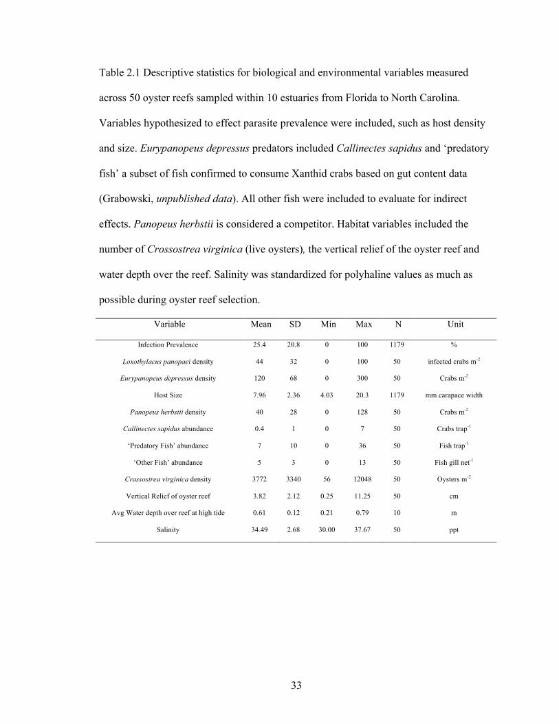
Table 2.1 Descriptive statistics for biological and environmental variables measured

across 50 oyster reefs sampled within 10 estuaries from Florida to North Carolina.

Variables hypothesized to effect parasite prevalence were included, such as host density

and size. Eurypanopeus depressus predators included Callinectes sapidus and ‘predatory

fish’ a subset of fish confirmed to consume Xanthid crabs based on gut content data

(Grabowski, unpublished data). All other fish were included to evaluate for indirect

effects. Panopeus herbstii is considered a competitor. Habitat variables included the

number of Crossostrea virginica (live oysters), the vertical relief of the oyster reef and

water depth over the reef. Salinity was standardized for polyhaline values as much as

possible during oyster reef selection.

Variable Mean SD Min Max N Unit

Infection Prevalence 25.4 20.8 0 100 1179 %

Loxothylacus panopaei density 44 32 0 100 50 infected crabs m-2

Eurypanopeus depressus density 120 68 0 300 50 Crabs m-2

Host Size 7.96 2.36 4.03 20.3 1179 mm carapace width

Panopeus herbstii density 40 28 0 128 50 Crabs m-2

Callinectes sapidus abundance 0.4 1 0 7 50 Crabs trap-1

‘Predatory Fish’ abundance 7 10 0 36 50 Fish trap-1

‘Other Fish’ abundance 5 3 0 13 50 Fish gill net-1

Crassostrea virginica density 3772 3340 56 12048 50 Oysters m-2

Vertical Relief of oyster reef 3.82 2.12 0.25 11.25 50 cm

Avg Water depth over reef at high tide 0.61 0.12 0.21 0.79 10 m

Salinity 34.49 2.68 30.00 37.67 50 ppt

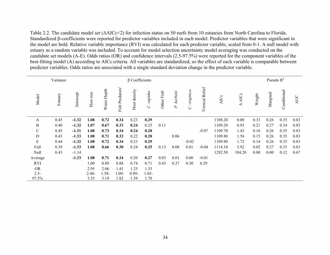
34

Table 2.2. The candidate model set (ΔAICc<2) for infection status on 50 reefs from 10 estuaries from North Carolina to Florida. Standardized β-coefficients were reported for predictor variables included in each model. Predictor variables that were significant in the model are bold. Relative variable importance (RVI) was calculated for each predictor variable, scaled from 0-1. A null model with estuary as a random variable was included. To account for model selection uncertainty model averaging was conducted on the candidate set models (A-E). Odds ratios (OR) and confidence intervals (2.5-97.5%) were reported for the component variables of the best-fitting model (A) according to AICc criteria. All variables are standardized, so the effect of each variable is comparable between predictor variables. Odds ratios are associated with a single standard deviation change in the predictor variable.

Variance β Coefficients Pseudo R2

Mod

el

Estu

ary

Inte

rcep

t

Hos

t siz

e

Wat

er D

epth

Fish

Pre

dato

rs'

Hos

t den

sity

C. s

apid

us

Oth

er F

ish'

P. h

erbs

tii

C. v

irgi

nica

Ver

tical

Rel

ief

AIC

c

Δ A

ICc

Wei

ght

Mar

gina

l

Con

ditio

nal

AU

C

A 0.45 -1.32 1.08 0.72 0.34 0.23 0.29 1108.20 0.00 0.33 0.26 0.35 0.83 B 0.40 -1.32 1.07 0.67 0.33 0.24 0.25 0.11 1109.20 0.93 0.21 0.27 0.34 0.83 C 0.45 -1.31 1.08 0.73 0.34 0.24 0.28 -0.07 1109.70 1.43 0.16 0.26 0.35 0.83 D 0.43 -1.33 1.08 0.71 0.32 0.22 0.28 0.06 1109.80 1.56 0.15 0.26 0.35 0.83 E 0.44 -1.32 1.08 0.72 0.34 0.23 0.29 -0.02 1109.90 1.72 0.14 0.26 0.35 0.83

Full 0.39 -1.33 1.08 0.66 0.30 0.24 0.25 0.13 0.08 0.01 -0.04 1114.10 5.92 0.02 0.27 0.35 0.83 Null 0.43 -1.14 1292.50 184.20 0.00 0.00 0.12 0.67

Average -1.33 1.08 0.71 0.34 0.20 0.27 0.03 0.01 0.00 -0.01 RVI 1.00 0.89 0.88 0.74 0.71 0.43 0.37 0.30 0.29 OR 2.95 2.06 1.41 1.25 1.33 2.5-

97.5% 2.48-3.55

1.58-3.19

1.09-1.82

0.99-1.59

1.05-1.70

35

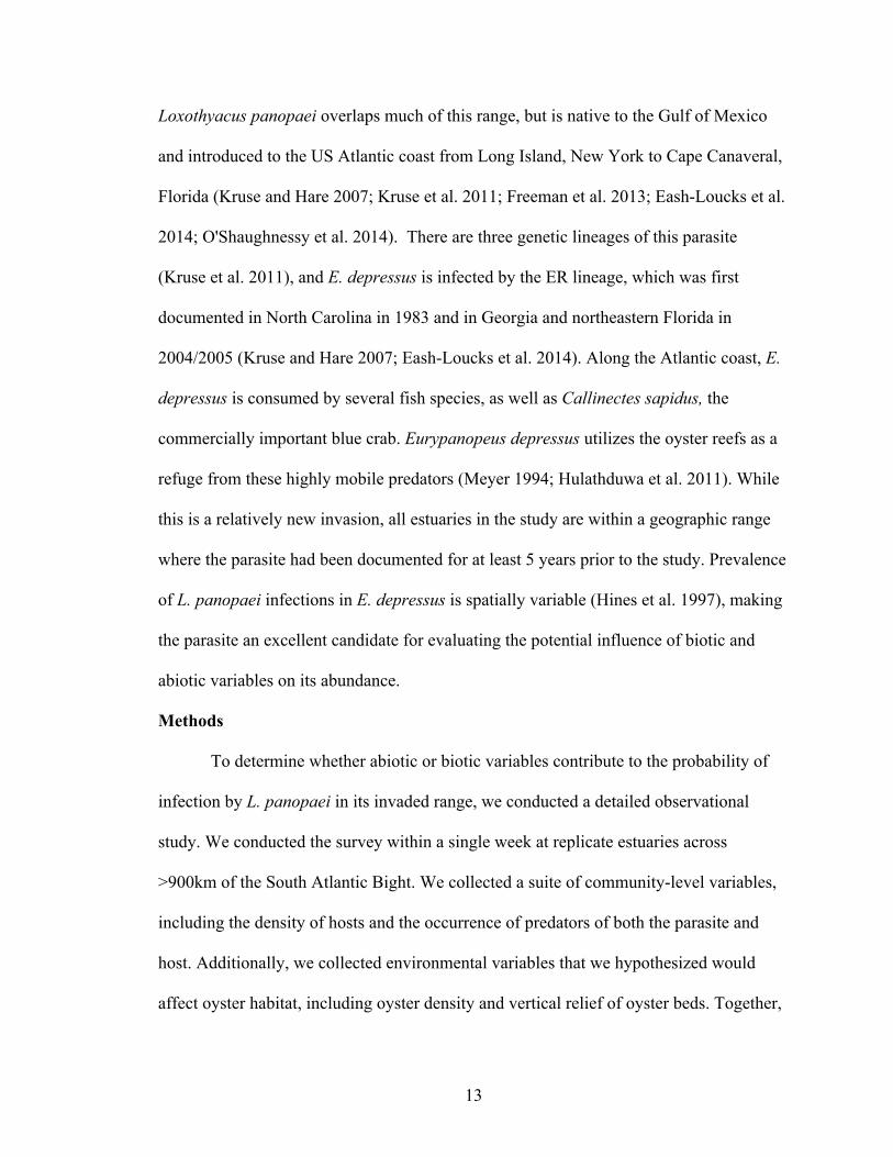
Fig 2.1 Map of the South Atlantic Bight indicating the average prevalence (± SD) of L.

panopaei infection in E. depressus across five reefs sampled in each of 10 estuaries (for

additional information see; (Byers et al. 2015).

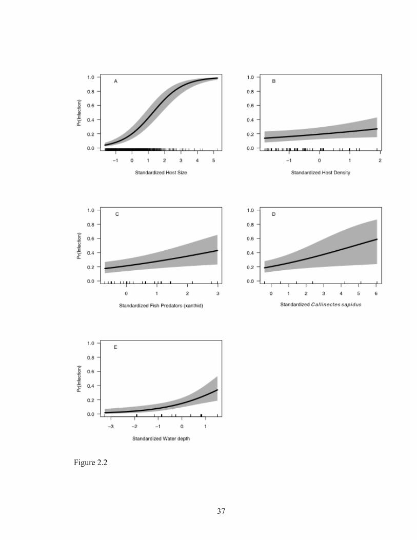
36

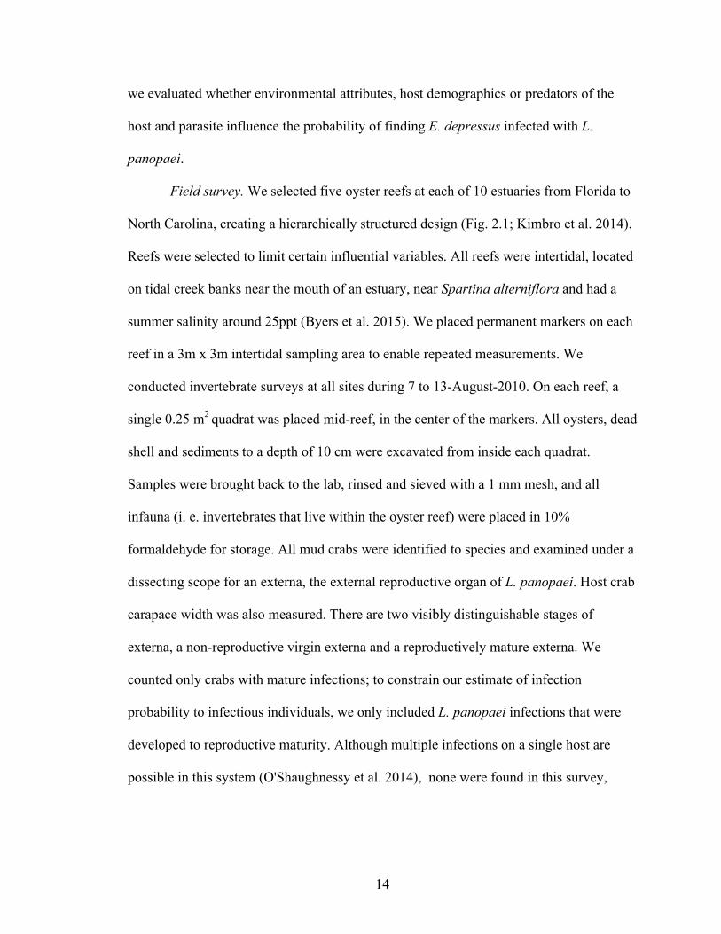
Fig 2.2 Probability of infection as a function of each predictor variable included in the

top model (model A in Table 2). 95% confidence intervals were calculated only

considering the fixed effects (grey shading). Vertical hash marks along the x-axis indicate

the spread of the data points used to fit the model. Differences in the number of hash

marks between variables reflect the scale and resolution of each measurement; for

example, water depth has fewer hash marks because there was only one measurement per

estuary. All predictor variables are standardized so that the effects of the variables are

readily comparable among each other, with every unit change associated with a single

standard deviation change in the predictor variable. A. Standardized host size measure as

carapace width (mm), B. Standardized host density measured as number of E. depressus

m-2, C. Standardized relative abundance of fish predators of small mud crabs (family

Xanthidae), D. Standardized relative abundance of Callinectes sapidus, E. Standardized

water depth over oyster reef (m).

37

Figure 2.2

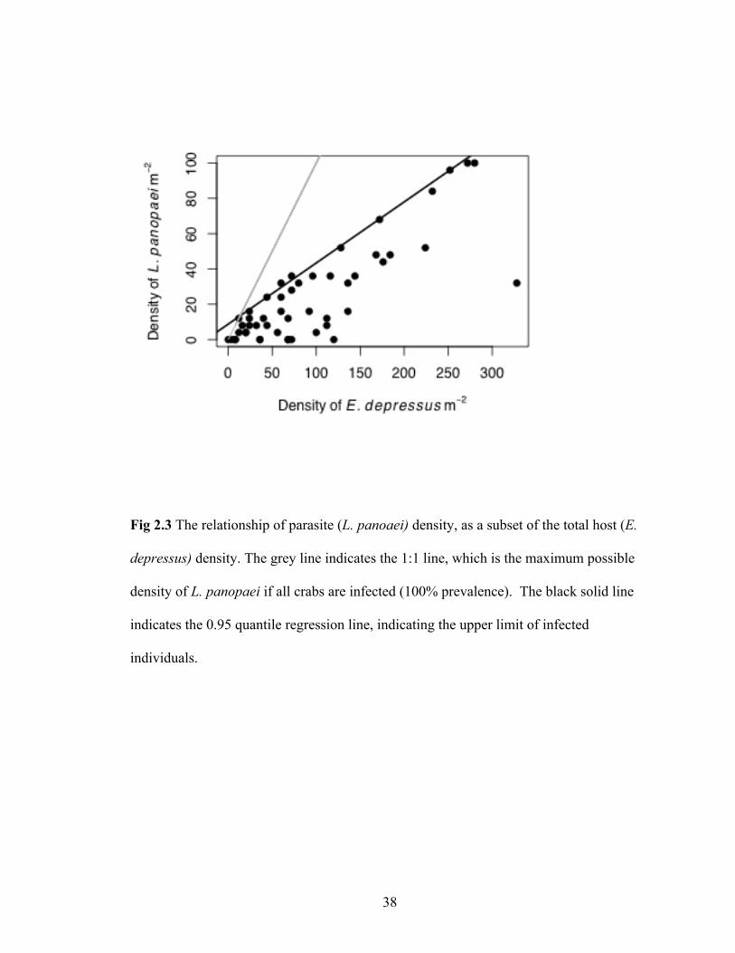
38

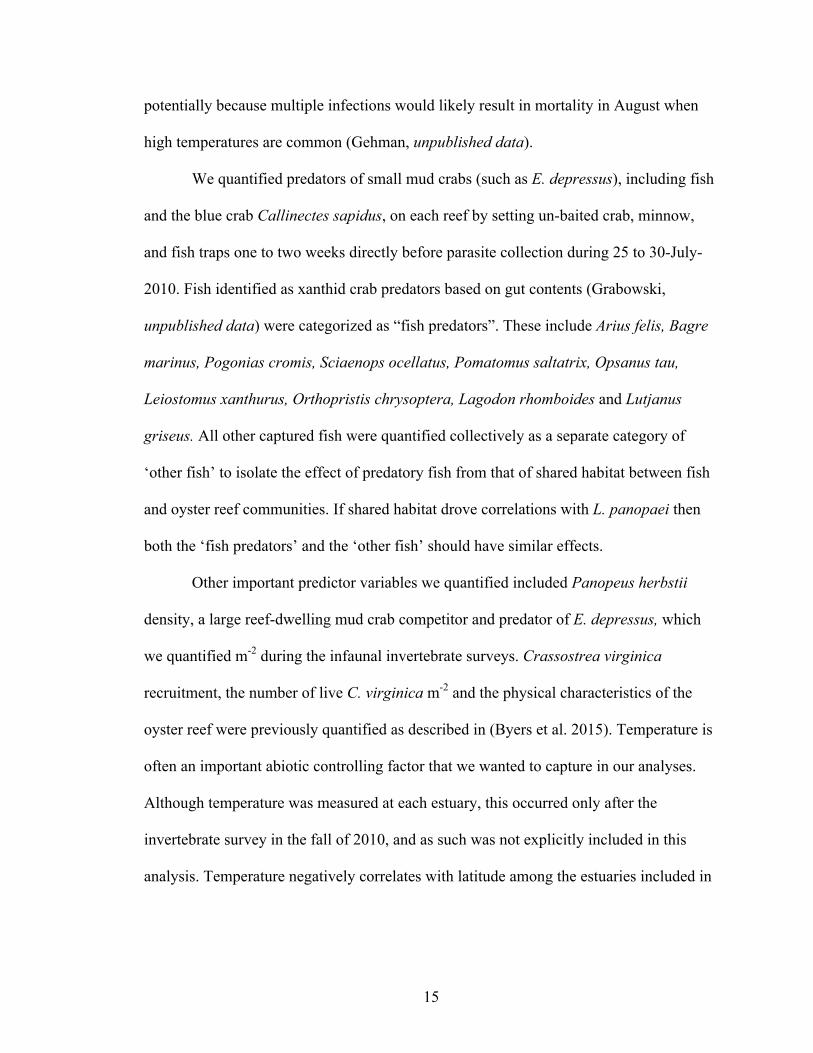
Fig 2.3 The relationship of parasite (L. panoaei) density, as a subset of the total host (E.

depressus) density. The grey line indicates the 1:1 line, which is the maximum possible

density of L. panopaei if all crabs are infected (100% prevalence). The black solid line

indicates the 0.95 quantile regression line, indicating the upper limit of infected

individuals.

39

CHAPTER 3

NON NATIVE PARASITE ENHANCES SUSCEPTIBILITY OF HOST TO NATIVE

PREDATORS2

2 Gehman, A.M., and J.E. Byers. To be submitted to Oecologia.

40

Summary

1. Parasites often alter host physiology and behavior, which may enhance predation

risk for infected hosts. Higher consumption of parasitized prey can in turn lead to

a less parasitized prey population (the healthy herd hypothesis).

2. Loxothylacus panopaei is a non-native castrating barnacle parasite on the mud

crab Eurypanopeus depressus along the Atlantic coast. We investigated whether

the predatory crab Callinectes sapidus and other predators preferentially feed on

E. depressus infected with L. panopaei and evaluated a mechanism behind prey

choice.

3. We evaluated prey choice through mesocosm experiments and a field tethering

experiment. Through behavioral trials we evaluated whether L. panopaei affects

E. depressus escape speed, making infected prey more susceptible to predator

attack.

4. We found that C. sapidus preferentially consumed infected E. depressus 3 to 1

over visibly uninfected E. depressus in the mesocosm experiments. Similarly,

infected E. depressus were consumed 1.4 to 1 over uninfected conspecifics in

field tethering trials. Contrary to our expectations, infected E. depressus ran faster

during laboratory trials than uninfected E. depressus, suggesting that quick

movement may not decrease predation risk, and seems instead to make prey more

vulnerable.

5. Ultimately, the preferential consumption of L. panopaei infected prey by C.

sapidus suggests that the predatory crab can lower L. panopaei abundance within

41

the local host population, potentially providing a biotic defense against this

invasive parasite.

Key-words Disease ecology, host-parasite, predator-prey, introduced species, marine

invertebrate, rhizocephalan, parasitism.

Introduction

With the increase in movement of species around the globe, through vectors such

as shipping and aquaculture, we are experiencing an era of new species interactions,

including invasions of novel parasites and diseases (Mack et al. 2000; Levine &

D'Antonio 2003). Invasive parasites, and more broadly emerging infectious diseases, can

have devastating effects on new hosts, depressing host populations to low levels (Garner

et al. 2006; Dunn & Hatcher 2015). This is likely due to the limited defenses of native

populations against novel parasites, leaving the population largely vulnerable (Hatcher,

Dick & Dunn 2012). However, native predators may help to mollify the influence of

invasive parasites on prey populations if they target parasitized prey. Although biotic

resistance, such as preferential predation on invasive species, is known to protect

communities from free-living invasive species (Byers 2002; deRivera et al. 2005), the

role of predators to affect invasive parasites in this manner has yet to be elucidated (Dunn

et al. 2012).

Selective consumption of infected prey by predators can occur if infected hosts

exhibit physiological or behavioral changes that increase their vulnerability (e.g. Lafferty

& Morris 1996). For example, nematode infected red grouse release more scent, leading

to higher predation rates on infected individuals (Hudson, Dobson & Newborn 1992).

42

Theory suggests that predators should be able to limit disease transmission within

populations (Hethcote et al. 2004; Wild et al. 2011; Chakraborty et al. 2015). For

example the ‘healthy herd’ hypothesis suggests that predators dampen disease

transmission, particularly when predators selectively feed on infected prey (Packer et al.

2003). However, preferential feeding on infected hosts does not always lead to decreased

infection prevalence (Duffy 2007). For example if predator avoidance behavior enhances

susceptibility there can be increased prevalence even with strong preferential feeding on

infected individuals (Duffy et al. 2011; Welch & Harwood 2011). Additionally, if the act

of predation increases disease transmission (e.g. “predator spreader” hypothesis) then

preferential predation on infected individuals can lead to increased infection prevalence

(Cáceres, Knight & Hall 2009). While preferential feeding on infected hosts has been

documented for a range of systems (Duffy et al. 2005; Duffy 2007; Cáceres et al. 2009;

Krkosek et al. 2011), preferential feeding on native hosts infected by an invasive parasite

has not been documented (Dunn et al. 2012).

Invasive parasites may be particularly likely to enhance vulnerability of their

hosts to native predators. Coevolution between native hosts and their parasites is

expected to evolve towards an optimum level of virulence, with the relative cost of

increased host mortality balanced with the benefit of increased reproductive output (Price

1980; Anderson & May 1982). The naïve host theory suggests that novel infections may

lead to the parasite overexploiting their new hosts (Cruz, Manolis & Wiley 1985;

Fassbinder-Orth, Barak & Brown 2013; Lymbery et al. 2014), which may leave both host

and parasite vulnerable to predators. In fact, for the invasive parasites with available

comparative measures of pathogenic effects, 85% showed increased pathogenicity in

43

naïve hosts (Lymbery et al. 2014). Pathogenicity may lead to disease behavior (e.g.

lethargy) and increased vulnerability to predators. Even when the parasite has a shared

coevolutionary history with the host, parasite range expansion into previously uninfected

areas of the host range can lead to overexploitation of the naïve host population (e.g.

Cudmore et al. 2010).

The United States Atlantic coast populations of the mud crab Eurypanopeus

depressus are invaded by a castrating Rhizocephalan barnacle parasite, Loxothylacus

panopaei (Reinhard & Reischman 1958; Kruse, Hare & Hines 2011). Rhizocephalans

often induce behavioral changes in their hosts, including decreasing infected host feeding

rates (O'Shaughnessy, Harding & Burge 2014; Toscano, Newsome & Griffen 2014), and

inducing movement of the host to risky positions to increase the spread of the parasite

offspring (Hoeg 1995). These behavioral alterations are also likely to enhance predation

risk in their hosts. L. panopaei is a native parasite of E. depressus in the Gulf of Mexico

and was introduced to the Chesapeake Bay in the 1960s in association with oyster

aquaculture (Van Engel et al. 1966). The parasite has since expanded its range north to

Long Island, New York and south to Cape Canaveral Florida, and was first reported in

Georgia 2004/2005 (Kruse & Hare 2007; Kruse et al. 2011; Freeman, Blakeslee &

Fowler 2013; Eash-Loucks, Kimball & Petrinec 2014). E. depressus population density

decreased following L. panopaei invasion in some regions (Andrews 1980; Eash-Loucks

et al. 2014), and infection prevalence in the invaded range is markedly higher than that

found in the native range (Hines, Alvarez & Reed 1997; Kruse & Hare 2007). E.

depressus utilizes oyster reefs as a refuge from predators (Meyer 1994; Hulathduwa et al.

2011), which include several fish and crab species (e.g. the blue crab Callinectes

44

sapidus). In this study we evaluate (A) whether the blue crab C. sapidus preferentially

feeds on E. depressus infected with L. panopaei; (B) whether E. depressus infected with

L. panopaei are more vulnerable to predation in the field; and (C) whether L. panopaei

impedes E. depressus movement, possibly increasing the vulnerability of both host and

parasite to predators.

Materials and methods

Collection Techniques

For all experiments described below, we collected E. depressus and C. sapidus from

Wassaw Sound, near Priests Landing, Savannah, GA (31°57’46.6”N, 81°00’47.9”W).

We collected C. sapidus using small fish traps baited with frozen chicken. To collect E.

depressus we collected oyster clumps at low tide and brought them back to the lab. In the

lab we removed mud and broke oyster clumps apart in a mesh basket to find E.

depressus. We collected healthy and infected E. depressus immediately prior to each

experiment; 27-29 June 2012 and 16-19 July 2012 for experiment (A), 21 July and 6

August 2014 for experiment (B), and 7 February 2013 for experiment (C).

We considered a host ‘infected’ if it was bearing a mature externa (the external

reproductive organ of the parasite, Fig. 3.1), and considered it “healthy’ if it was non-

externa bearing. There is an internal phase of infection, so some crabs labeled healthy

were likely internally infected with an incipient infection, making any difference found

between healthy and infected individuals in our study a likely conservative estimation of

the parasite’s effect. Throughout the manuscript we will refer to a visibly healthy E.

depressus as a ‘healthy host’ and an E. depressus visibly infected with L. panopaei as an

‘infected host’. For all experiments, attempts were made to keep host size similar,

45

however the size differences between healthy and infected hosts reflect those observed in

the field (Table 3.1, Gehman et al, unpublished data). Prior to each experiment we kept

infected and healthy hosts in separate flow-through seawater tables to prevent parasite

transmission.

A. Do predatory crabs preferentially consume infected hosts over healthy hosts

(mesocosm study)? To quantify consumption of infected and healthy E. depressus by

predatory C. sapidus, we placed 5 healthy and 5 infected E. depressus hosts into a 19L

tank and exposed them to C. sapidus. For habitat, each tank contained a single layer of

sun bleached local oyster shell and its own separate delivery of flowing seawater which

was kept at ~19L/half hour throughout the trial. We allowed E. depressus to settle for

half an hour and then we placed a single C. sapidus predator (80-90mm carapace width)

in each tank. Light-dark cycles were set to 15 hours of dark and 9 hours of light. We ran

each trial for 7 days and monitored them twice a day, once just prior to turning off the

lights and once immediately after the lights turned on. For staging purposes, we

conducted the full experiment twice, over two consecutive time blocks with 10 replicate

tanks in each block (n=20 C. sapidus for the whole experiment).

At each monitoring point we removed the predatory crabs from the tanks and

placed them in a separate tank with seawater. We carefully examined the contents of each

tank, removing each oyster shell one at a time to examine them for presence of the

healthy and infected hosts. We recorded the number that were alive, dead, and missing,

and removed the dead. We considered crabs consumed if they were missing. We

considered crabs dead if they did not move in response to direct stimulus (only two crabs

were recorded in this category over the course of the experiment). To keep the

46

availability of healthy and infected prey even across time, we brought the total number of

available prey back to 5 healthy and 5 infected hosts at each monitoring point (twice a

day). After tabulating we allowed the infected and healthy hosts to acclimate for a half an

hour before returning the same predator to each tank. We quantified the cumulative

number of infected and healthy hosts consumed by each predator over the course of the

full 7-day experiment.

We performed individual χ2 tests on each replicate predator to compare the

preference of each crab for healthy or infected hosts. To determine whether crab

preference was homogenous among replicates we conducted an I2 analysis, which

describes the proportion of the predator preference estimate that is driven by

heterogeneity between individuals (Higgins & Thompson 2002). The I2 was relatively

low within each time block and similar between each time block (time block one I2= 44,

time block two I2 = 47). Therefore the two time blocks were combined together for an

analysis to test the null hypothesis of no preference by predatory crabs for the infected or

healthy hosts. We used R 3.1.3 for this and all subsequent statistical analysis (R

Development Core Team 2015).

B. Do predators preferentially consume infected hosts over healthy hosts (field study)?

To evaluate whether infected hosts were preferentially consumed over healthy hosts by a

full suite of ambient predators in the field, we tethered healthy and infected hosts to a

30.5 cm long PVC pole with a 25.4 cm monofilament line. The tether line was then glued

to the back of healthy and infected hosts carapace with Loclite® super glue (Fig. 3.2).

Glue was allowed to dry for approximately 5 minutes. To assure that all host crabs were

47

satisfactorily attached to their tethers, host crabs were kept for 24 hours in the flow-

through system prior to placement in the field.

During low tide we secured the PVC poles at 0.5m intervals within a mid-

intertidal oyster reef at Priests Landing, near the collection site of the crabs. To account

for the effect of location, we alternated healthy and infected crabs systematically along

the reef. We placed approximately 20 infected and 20 healthy crabs in the field for each

of 5 trials (n=93 healthy and n=95 infected hosts), blocked by date. Each trial lasted ~12

hours, starting on a late afternoon low tide and ending the following low tide. Although

tethering limited host movement, crabs were still able to move into the oyster reef to hide

from predators (Fig 3.2A and B). At collection we noted mortality, which was quantified

by loss of crabs, as well as recovery of crab remnants (Fig 3.2D). We conducted trials on

two adjacent reefs. We tested for the effect of blocking by reef and found no effect, so we

pooled the results from the two reefs together for all statistical analysis. Because infected

and healthy crabs were different sizes we explicitly included size to test the effect of size

on predation risk. We fit a generalized linear mixed effects model with a binomial

response (dead or alive), date of tethering trial as the random effect and size and infection

status and their interaction as fixed effects.

C. Are infected hosts slower than healthy hosts? To test whether infected hosts were

slower than healthy hosts, as a possible factor contributing to differential consumption,

we conducted movement experiments in the lab. We quantified the time for a crab to

move down an exposed runway to the end. To induce linear movement by each crab we

created a standardized exposed runway, composed of a PVC tube cut in half lengthwise,

which was submerged into artificial seawater in a container. To examine whether

48

exposure distance altered escape behavior, we ran two separate movement experiments,

differing only in the length of runway available. Thus, for the first trial the runway was

220mm from the center point to either end and for the second trial the runway was

94mm. For all experimental runs we hand placed a single individual in the middle of the

runway and recorded its movements and the time it took to reach the end of the runway

with a camera suspended above the tank. We ran 20 healthy and 16 infected hosts along

the long runway, and 19 healthy hosts and 10 infected hosts individually along the short

runway. We analyzed each runway length experiment separately using an ANOVA,

testing the effect of infection status on speed (mm/s) for each experiment.

Results

A. Do predatory crabs preferentially consume infected hosts over healthy hosts

(mesocosm study)? Predatory crabs consumed three times as many infected hosts on

average than healthy hosts (Fig. 3.3, χ2=33.3, p<<0.001, I2=47.2). Every one of the C.

sapidus individuals consumed more infected E. depressus than uninfected, with the diet

of each C. sapidus averaging 75% E. depressus infected with L. panopaei (± 1.7, SD).

Overall, 120 infected hosts were consumed through the course of this experiment,

whereas only 36 healthy crabs were consumed.

B. Do predators preferentially consume the infected hosts over the healthy host (field

study)? Infected hosts were 43% less likely to survive a single high tide cycle than

healthy hosts (Fig. 3.4, odds ratio=0.43, p=0.02). The interaction between host size and

infection status was non-significant (β=-0.01, p=0.97) so it was removed from the

analysis. Across both treatments, smaller host crabs were less likely to survive a single

high tide cycle, and the odds of survival increased 173% for every 1.1mm increase in

49

carapace width (Fig. 3.4, odds ratio =1.73, p=0.002). Therefore, even after controlling for

the effect of size there remained an effect of infection prevalence on survival.

C. Are infected hosts slower than healthy hosts? Regardless of runway length, infected

hosts moved approximately twice as fast to the end of the PVC tube than healthy hosts in

both experiments (long runway, F=8.5, df=1, MS=1323, p = 0.006, short runway, F=14.9,

df=1, MS= 2565, p = 0.001, Fig. 5).

Discussion

Parasitic infection by L. panopaei enhances predator consumption of E. depressus

by up to 3-fold in mesocosms (Fig. 3.3) and 1.4 to 1 in the field (Fig. 3.4). Contrary to

our hypothesis, the enhanced consumption of infected hosts is not seemingly due to lower

escape speeds. We had surmised that either increased drag from the externa on the

infected crab’s abdomen or infection-induced lethargy would slow the infected host.

Rather, our experiment designed to isolate this behavioral mechanism showed that

infected crabs were twice as fast (Fig. 3.5), yet still more vulnerable to predators. Thus

heightened vulnerability to consumption of infected hosts occurs in spite of, or because

of, faster movement. Indeed, it is possible that quick movement could increase the

visibility (e.g. Hemmi & Pfeil 2010), or other sensory cues (e.g. mechanosensory

(Schwalbe, Bassett & Webb 2012)), of the prey to their predators

The differentially high consumptive pressure on infected hosts suggests the

healthy herd mechanism could be acting within this system. Evaluated at a mechanistic

level, infected crabs are being differentially removed from the environment by predators

over their healthy counterparts (Fig. 3.3). However, across estuaries there is a positive

relationship between predator abundance and infection prevalence (Gehman et. al.

50

unpublished data), which superficially might lead to the opposite conclusion (i.e. that

predators preferentially consume uninfected hosts). Given the preferential consumption

of infected individuals that we document, this positive association at a large scale must be

driven by other mechanisms. For example, the predator and prey may be positively

associated with a third environmental variable (e.g. ocean currents). Alternatively, the

positive association between the predatory crab and its prey at a regional scale may

indicate that C. sapidus are moving to areas within the estuary with higher infection

prevalence to take advantage of easy prey items (Sih 1982; 2005; Wieters et al. 2008).

Prey size is an important factor for prey survival, with many prey reaching a

refuge from predators at larger sizes e.g. (McLennan et al. 2004). In our study, host

carapace width significantly increased host survival and had a similar positive effect on

infected and healthy hosts (Fig. 3.4). However, for any given carapace width, infected

crabs have lower survival than healthy crabs (Fig. 3.4); a trend that holds across all

carapace widths as signified by the non-significant interaction of infection status and

carapace width. Size determines dominance in many crab species (Somers & Nel 1998;

Shervette & Perry 2004) and refuge dominance is important for crab survival (Beck

1995; Shervette & Perry 2004; Hulathduwa et al. 2011). Therefore increased survival

with size suggests that larger E. depressus, regardless of infection status, are able to

dominate refuge use over their smaller counterparts, which may account for the strong

effect of increasing size on survival.

The predator used in our mesocosm trials, the blue crab C. sapidus, is a voracious

predator, and this is not the first time it has been implicated as biological resistance to

invasion. C. sapidus preferentially consumes Carcinus maenus, the invasive European

51

green crab, and high predation rates have likely inhibited the southern spread of C.

maenus (deRivera et al. 2005). The preferential feeding on infected E. depressus by C.

sapidus we found in this study suggests that this predator has the potential to provide a

biotic defense against this invasive parasite. Specifically, the preferential feeding on L.

panopaei-infected E. depressus by C. sapidus suggests that the predators may be able to

help limit the spread of this invasive parasite. L. panopaei infection prevalence varies

substantially along the Atlantic coastline (Hines et al. 1997; Kruse & Hare 2007; Kruse et

al. 2011; Freeman et al. 2013), and variation in predation pressure between sites may

affect infection prevalence. In this era of increased biological invasions that in turn

increase novel species interactions (Mack et al. 2000; Levine & D'Antonio 2003), there is

a great need to identify how novel species will interact with the community they are

invading. The results from this project help to highlight the importance of understanding

how interactions between organisms, such as predation by predators, can likely influence

the prevalence and abundance that novel parasites are able to achieve.

Data Accessibility

Data will be archived on Dryad prior to publication.

Acknowledgements

We thank A. Penn, S. Perry, R. Smith, Z. Holmes, A. Calfee, and R. Usher for field and

lab assistance. We thank the Byers and Osenberg labs for discussion and R. D. Harris for

help with the conceptual diagram. Thanks to my committee J. Porter, S. Altizer, V.

Ezenwa and W. Fitt for valuable guidance. We thank Jonathan Little, Kevin Ruddell,

Heather Kroll and 30 other supporters for significant support of this research through the

52

#SciFund Challenge. Support also came from the Odum School of Ecology. The lead

author is a fellow with the Wormsloe Institute for Environmental History.

Literature Cited

Anderson, R.M. & May, R.M. (1982) Coevolution of hosts and parasites. Parasitology,

85 (Pt 2), 411–426.

Andrews, J.D. (1980) A Review of Introductions of Exotic Oysters and Biological

Planning for New Importations. Marine Fisheries Review, 42, 1–11.

Beck, M.W. (1995) Size-specific shelter limitation in stone crabs: a test of the

demographic bottleneck hypothesis. Ecology, 76, 968–980.

Byers, J.E. (2002) Physical habitat attribute mediates biotic resistance to non-indigenous

species invasion. Oecologia, 130, 146–156.

Cáceres, C.E., Knight, C.J. & Hall, S.R. (2009) Predator-spreaders: predation can

enhance parasite success in a planktonic host-parasite system. Ecology, 90, 2850–2858.

Chakraborty, S., Kooi, B.W., Biswas, B. & Chattopadhyay, J. (2015) Revealing the role

of predator interference in a predator-prey system with disease in prey population.

Ecological Complexity, 21, 100–111.

Cruz, A., Manolis, T. & Wiley, J.W. (1985) The Shiny Cowbird: a brood parasite

expanding its range in the Caribbean region. Ornithological Monographs, 607–620.

Cudmore, T.J., Björklund, N., Carroll, A.L. & Staffan Lindgren, B. (2010) Climate

change and range expansion of an aggressive bark beetle: evidence of higher beetle

53

reproduction in naïve host tree populations. Journal of Applied Ecology, 47, 1036–1043.

deRivera, C.E., Ruiz, G.M., Hines, A.H. & Jivoff, P. (2005) Biotic Resistance to

Invasion: Native Predator Limits Abundance and Distribution of an Introduced Crab.

Ecology, 86, 3364–3376.

Duffy, M.A. (2007) Selective predation, parasitism, and trophic cascades in a bluegill-

Daphnia-parasite system. Oecologia, 153, 453–460.

Duffy, M.A., Hall, S.R., Tessier, A. & Huebner, M. (2005) Selective predators and their

parasitized prey: are epidemics in zooplankton under top-down control? Limnology and

Oceanography, 50, 412–420.

Duffy, M.A., Housley, J.M., Penczykowski, R.M., Cáceres, C.E. & Hall, S.R. (2011)

Unhealthy herds: indirect effects of predators enhance two drivers of disease spread.

Functional Ecology, 25, 945–953.

Dunn, A.M. & Hatcher, M.J. (2015) Parasites and biological invasions: parallels,

interactions, and control. Trends in Parasitology, 31, 189–199.

Dunn, A.M., Torchin, M.E., Hatcher, M.J., Kotanen, P.M., Blumenthal, D.M., Byers,

J.E., Coon, C.A.C., Frankel, V.M., Holt, R.D., Hufbauer, R.A., Kanarek, A.R.,

Schierenbeck, K.A., Wolfe, L.M. & Perkins, S.E. (2012) Indirect effects of parasites in

invasions (ed C Fox). Functional Ecology, 26, 1262–1274.

Eash-Loucks, W.E., Kimball, M.E. & Petrinec, K.M. (2014) Long-term changes in an

estuarine mud crab community: evaluating the impact of non-native species. Journal of

54

Crustacean Biology, 34, 731–738.

Fassbinder-Orth, C.A., Barak, V.A. & Brown, C.R. (2013) Immune Responses of a

Native and an Invasive Bird to Buggy Creek Virus (Togaviridae: Alphavirus) and Its

Arthropod Vector, the Swallow Bug (Oeciacus vicarius). PLoS ONE, 8, e58045.

Freeman, A.S., Blakeslee, A.M.H. & Fowler, A.E. (2013) Northward expansion of the

rhizocephalan Loxothylacus panopaei (Gissler, 1884) in the northwest Atlantic. Aquatic

Invasions, 8, 347–353.

Garner, T.W.J., Perkins, M.W., Govindarajulu, P., Seglie, D., Walker, S., Cunningham,

A.A. & Fisher, M.C. (2006) The emerging amphibian pathogen Batrachochytrium

dendrobatidis globally infects introduced populations of the North American bullfrog,

Rana catesbeiana. Biology Letters, 2, 455–459.

Hatcher, M.J., Dick, J.T.A. & Dunn, A.M. (2012) Disease emergence and invasions.

Functional Ecology, 26, 1275–1287.

Hemmi, J.M. & Pfeil, A. (2010) A multi-stage anti-predator response increases

information on predation risk. Journal of Experimental Biology, 213, 1484–1489.

Hethcote, H.W., Wang, W., Han, L. & Ma, Z. (2004) A predator-prey model with

infected prey. Theoretical Population Biology, 66, 259–268.

Higgins, J.P.T. & Thompson, S.G. (2002) Quantifying heterogeneity in a meta-analysis.

Statistics in Medicine, 21, 1539–1558.

Hines, A.H., Alvarez, F. & Reed, S. (1997) Introduced and native populations of a marine

55

parasitic castrator: variation in prevalence of the rhizocephalan Loxothylacus panopaei in

xanthid crabs. Bulletin of Marine Science, 61, 197–214.

Hoeg, J.T. (1995) The biology and life cycle of the rhizocephala (Cirripedia). Journal of

Marine Biological Association of the UK, 75, 517–550.

Hudson, P.J., Dobson, A. & Newborn, D. (1992) Do parasites make prey vulnerable to

predation? Red grouse and parasites. Journal of Animal Ecology, 61, 681–692.

Hulathduwa, Y.D., Stickle, W.B., Aronhime, B. & Brown, K.M. (2011) Differences in

refuge use are related to predation risk in estuarine crabs. Journal of Shellfish Research,

30, 949–956.

Krkosek, M., Connors, B.M., Ford, H., Peacock, S., Mages, P., Ford, J.S., Morton, A.,

Volpe, J.P., Hilborn, R., Dill, L.M. & Lewis, M.A. (2011) Fish farms, parasites, and

predators: implications for salmon population dynamics. Ecological applications, 21,

897–914.

Kruse, I. & Hare, M.P. (2007) Genetic diversity and expanding nonindigenous range of

the rhizocephalan Loxothylacus panopaei parasitizing mud crabs in the western north

Atlantic. Journal Of Parasitology, 93, 575–582.

Kruse, I., Hare, M. & Hines, A.H. (2011) Genetic relationships of the marine invasive

crab parasite Loxothylacus panopaei: an analysis of DNA sequence variation, host

specificity, and distributional range. Biological Invasions, 14, 701–715.

Lafferty, K.D. & Morris, A.K. (1996) Altered behavior of parasitized Killifish increases

56

susceptibility to predation by bird final hosts. Ecology, 77, 1390–1397.

Levine, J.M. & D'Antonio, C.M. (2003) Forecasting biological invasions with increasing

international trade. Conservation Biology, 17, 322–326.

Lymbery, A.J., Morine, M., Kanani, H.G., Beatty, S.J. & Morgan, D.L. (2014) Co-

invaders: The effects of alien parasites on native hosts. International Journal for

Parasitology: Parasites and Wildlife, 3, 171–177.

Mack, R.N., Simberloff, D., Lonsdale, W.M., Evans, H., Clout, M. & Bazzaz, F.A.

(2000) Biotic Invasions: Causes, Epidemiology, Global Consequences, and Control.

Ecological Applications, 10, 689–710.

McLennan, J.A., Dew, L., Miles, J., Gillingham, N. & Waiwai, R. (2004) Size matters:

predation risk and juvenile growth in North Island brown kiwi (Apteryx mantelli). New

Zealand Journal of Ecology, 28, 241–250.

Meyer, D. (1994) Habitat partitioning between the xanthid crabs Panopeus herbstii and

Eurypanopeus depressus on intertidal oyster reefs (Crassostrea virginica) in southeastern

North Carolina. Estuaries and Coasts, 17, 674–679.

O'Shaughnessy, K.A., Harding, J.M. & Burge, E.J. (2014) Ecological effects of the

invasive parasite Loxothylacus panopaei on the flatback mud crab Eurypanopeus

depressus with implications for estuarine communities. Bulletin of Marine Science, 90,

611–621.

Packer, C., Holt, R.D., Hudson, P.J., Lafferty, K.D. & Dobson, A.P. (2003) Keeping the

57

herds healthy and alert: implications of predator control for infectious disease. Ecology

Letters, 6, 797–802.

Price, P.W. (1980) Evolutionary biology of parasites. Monographs in population biology,

15, 1–237.

R Development Core Team. (2015) R: A language and environment for statistical

computing.

Reinhard, E. & Reischman, P. (1958) Variation in Loxothylacus panopaei (Gissler), a

common Sacculinid parasite of mud crabs, with the description of Loxothylacus

perarmatus, n. sp. The Journal of Parasitology, 44, 93–97.

Schwalbe, M.A.B., Bassett, D.K. & Webb, J.F. (2012) Feeding in the dark: lateral-line-

mediated prey detection in the peacock cichlid Aulonocara stuartgranti. Journal of

Experimental Biology, 215, 2060–2071.

Shervette, V.R. & Perry, H.M. (2004) Factors influencing refuge occupation by stone

crab Menippe adina juveniles in Mississippi Sound. Journal of Crustacean Biology, 24,

652–665.

Sih, A. (1982) Optimal Patch Use: Variation in Selective Pressure for Efficient Foraging.

American Naturalist, 120, 666–685.

Sih, A. (2005) Predator-prey space use as an emergent outcome of a behavioral response

race. Ecology of predator-prey interactions (eds P. Barbosa & I. Castellanos) Ecology of

predator-prey interactions.

58

Somers, M.J. & Nel, J.A.J. (1998) Dominance and population structure of freshwater

crabs (Potamonautes perlatus Milne Edwards). South African Journal of Zoology, 33, 31–

36.

Toscano, B.J., Newsome, B. & Griffen, B.D. (2014) Parasite modification of predator

functional response. Oecologia, 175, 345–352.

Van Engel, W., Dillon, W.A., Zwerner, D. & Eldridge, D. (1966) Loxothylacus Panopaei

(cirripedia, Sacculinidae) an Introduced Parasite on a Xanthid Crab in Chesapeake Bay,

U.S.A. Crustaceana, 10, 110–112.

Welch, K.D. & Harwood, J.D. (2011) Predator-pathogen interactions: synergy between

mortality causes and failure of the healthy herds hypothesis. Functional Ecology, 25,

943–944.

Wieters, E.A., Gaines, S.D., Navarrete, S.A., Blanchette, C.A. & Menge, B.A. (2008)

Scales of Dispersal and the Biogeography of Marine Predator‐Prey Interactions.

American Naturalist, 171, 405–417.

Wild, M., Thompson Hobbs, N., Graham, M. & Miller, M. (2011) The role of predation

in disease control: A comparison of selective and nonselective removal on prion disease

dynamics in deer. Journal of Wildlife Diseases, 47, 78.

59

Table 3.1 Mean (SD) size of the healthy E. depressus and E. depressus infected by L.

panopaei that we offered to C. sapidus for consumption (A) and were tethered in the field

(B) to test for the effect of parasite infection status on infected and healthy host

vulnerability to predators.

Infectedhost-mm Healthyhost-mm

Mesocosm 9.78(1.35) 7.78(1.13)

Field 9.96(1.04) 9.52(1.08)

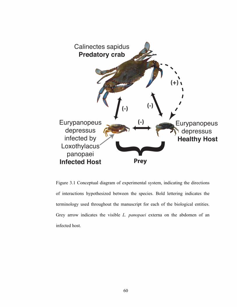
60

Figure 3.1 Conceptual diagram of experimental system, indicating the directions

of interactions hypothesized between the species. Bold lettering indicates the

terminology used throughout the manuscript for each of the biological entities.

Grey arrow indicates the visible L. panopaei externa on the abdomen of an

infected host.

Eurypanopeus depressus infected by

Loxothylacus panopaei

Infected Host

Eurypanopeus depressus

Healthy Host

Calinectes sapidusPredatory crab

}Prey

(-)

(-)

(-)

(+)

61

Figure 3.2 Eurypanopeus depressus tethered in an oyster reef at Priest Landing,

Savannah, GA for a field predation trial. A. An E. depressus on its tether moving

across the oyster reef (black arrow), B. towards a crevice within an oyster clump

to hide inside (yellow arrow), demonstrating that E. depressus on the tethers were

able to hide from predators. C. A live E. depressus shortly after being placed in

the field. D. The empty carapace of a partially consumed E. depressus still on

tether. The eyestalks (black arrow) remain with the carapace, indicating that the

crab did not molt.

A B

C D

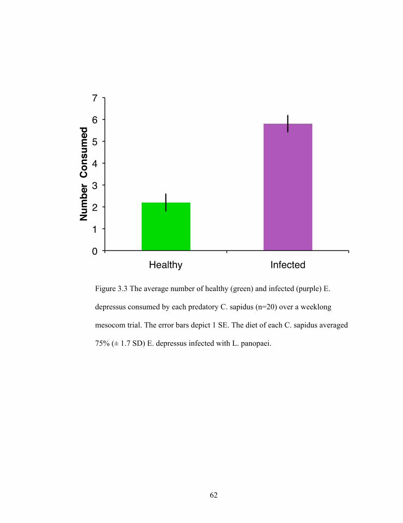
62

Figure 3.3 The average number of healthy (green) and infected (purple) E.

depressus consumed by each predatory C. sapidus (n=20) over a weeklong

mesocom trial. The error bars depict 1 SE. The diet of each C. sapidus averaged

75% (± 1.7 SD) E. depressus infected with L. panopaei.

0

1

2

3

4

5

6

7

Healthy Infected

Num

ber

Con

sum

ed

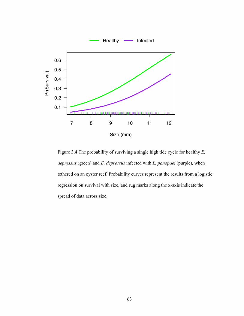
63

Figure 3.4 The probability of surviving a single high tide cycle for healthy E.

depressus (green) and E. depressus infected with L. panopaei (purple), when

tethered on an oyster reef. Probability curves represent the results from a logistic

regression on survival with size, and rug marks along the x-axis indicate the

spread of data across size.

7 8 9 10 11 12

0.1

0.2

0.3

0.4

0.5

0.6

Size (mm)

Pr(S

urvi

val)

Healthy Infected

64

Figure 3.5 Speed of healthy E. depressus (green) and infected E. depressus

(purple) running 220mm (long runway) and 94mm (short runway) along a PVC

tube. Error bars are standard errors and the number of replicates in each study are

listed along the x-axis.

●

●

●

●

010

2030

4050

Spee

d (m

m/s

)

Healthy Infected Healthy Infected

Long Runway Short Runway

20 16 19 10

● Infected

65

CHAPTER 4

INCREASED TEMPERATURES DIFFERENTIALLY AFFECT INVASIVE

PARASITE, FREEING HOST FROM INFECTION3

3 Gehman, A.M., R.J. Hall and J.E. Byers. To be submitted to Science.

66

Abstract

Hosts and parasites are coupled systems, but each can respond differently to changes in

environmental variables like temperature. Temperature influences the physiology of hosts

and parasites’ thermal responses, differentially shift with climate change has been widely

speculated on, but combined empirical and modeling work is critically needed to predict

parasite response to climate change. Here we explicitly quantify thermal response curves

encompassing the thermal breadth of the host and parasite, yielding an unprecedented

dataset for a marine system. We found a thermal mismatch in survival optima between

infected and uninfected hosts, with infected host demonstrating unexpected thermal

performance optima at lower temperatures then the uninfected host. We parameterized a

physiologically based epidemiological model to predict the sensitivity of this host-

parasite system to future climate warming scenarios. The model accurately predicted the

observed annual cycles and seasonality in the host-parasite system. Under plausible

warming scenarios, parasite prevalence declined with summer temperature, with parasite

local extinction predicted given mean 3º C warming. This work suggests that hosts might

benefit from seasonal mismatch in thermal optima for host, and further highlights the

need to explicitly include host and parasite thermal performance curves to predict

infection responses to climate change.

Introduction, Results and Discussion

Environmental change fundamentally affects individual animals, and individual

response to climate alters how species interact with each other. These changes in species

interactions are the key link between climate effects on individuals and the responses of

67

communities. The intimate association between parasites and their host make them well

suited for evaluating how environmental change alters species interactions. For example,

warming in temperate regions is predicted to increase the distribution and activity of

ectothermic vectors of human pathogens, which coupled with an increase in vector and

parasite development rates might result in higher transmission potential (LaDeau et al.

2015, Ren et al. 2016). Together, the increase in vector borne diseases as the climate

changes has led some to argue that a warmer world will be a sicker world (Harvell et al.

2002). Although, the generality of this hypothesis is under debate (Rohr et al. 2011,

Altizer et al. 2013), since temperature can differentially influence within-host and

between-host processes in non-additive ways, making the net effect of warming difficult

to predict. For example, greater parasite reproduction with temperature may not change

parasite dynamics if increased temperature also enhances parasite induced mortality in

the host (Anderson and May 1979). Empirical data are limited, even in the best studied

human disease systems (Mordecai et al. 2013, LaDeau et al. 2015), and a comprehensive

analysis of the effects of temperature on multiple stages of infection within a single host

has not yet been accomplished.

Temperature is one of the most important factors affecting the performance of

ectotherms, with practically all physiological and behavioral attributes sensitive to

temperature (Dell et al. 2011, Amarasekare and Sifuentes 2012). Ectothermic response to

temperature is predictable, and can be described by thermal performance curves (Huey

and Kingsolver 1989). For many species, development does not occur below a lower

threshold temperature (Tmin), increases to an optimum (Topt) and rapidly decreases above

the optimum to zero (Tmax). Despite extensive knowledge of these physiological

68

responses, studies that consider temperature effects on host-parasite interactions focus on

increasing relationship prior to Topt, but ignore the non-linear responses to temperature on

parasite development and reproduction (but see (Molnár et al. 2012, Mordecai et al.

2013)). Parasites of ectothermic hosts are likely have the same non-linear rate responses

to temperature as their free-living hosts, and empirical evidence to explore this pattern is

crucially needed to predict population dynamic responses to warming (Rohr et al. 2011,

Altizer et al. 2013).

We test the predictions that hosts and parasites survival and parasite reproduction will

respond non-linearly to temperature, and that host survival and parasite production might

be optimized at different temperatures. We focus on a host-parasite system that exhibits

seasonal variation in infection prevalence (O'Shaughnessy et al. 2014b), and whose

biogeographic spread might be limited by high summer temperatures (Kruse et al. 2011).

Eurypanopeus depressus is an abundant oyster reef-dwelling crab that is infected with an

invasive rhizocephalan parasite, Loxothylacus panopaei. Parasites are directly

transmitted with a free-living stage that recruits to hosts (detailed lifecycle in supporting

online material; SOM). There are two distinct stages of L. panopaei infection: exposed

hosts, which are infected but the parasite is non-reproductive, and infected hosts, in

which the parasite is reproductive and releasing infective stages. We conducted

laboratory experiments in Savannah, GA, in which we manipulated temperature and

quantified thermal performance curves by subjecting uninfected hosts (susceptible) and

two infection stages (exposed and infected; Figure 4.1) to temperatures encompassing the

observed thermal breadth of the host and parasite in coastal Georgia.

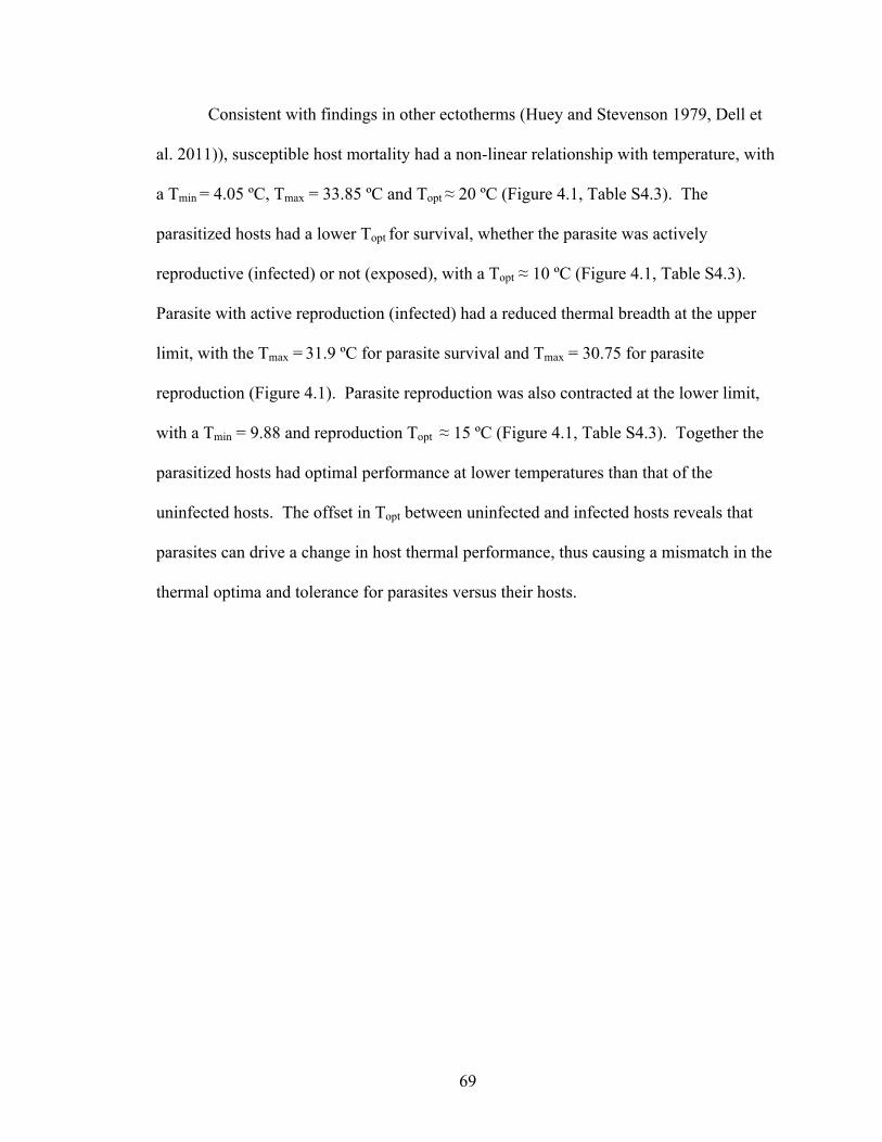
69

Consistent with findings in other ectotherms (Huey and Stevenson 1979, Dell et

al. 2011)), susceptible host mortality had a non-linear relationship with temperature, with

a Tmin = 4.05 ºC, Tmax = 33.85 ºC and Topt ≈ 20 ºC (Figure 4.1, Table S4.3). The

parasitized hosts had a lower Topt for survival, whether the parasite was actively

reproductive (infected) or not (exposed), with a Topt ≈ 10 ºC (Figure 4.1, Table S4.3).

Parasite with active reproduction (infected) had a reduced thermal breadth at the upper

limit, with the Tmax = 31.9 ºC for parasite survival and Tmax = 30.75 for parasite

reproduction (Figure 4.1). Parasite reproduction was also contracted at the lower limit,

with a Tmin = 9.88 and reproduction Topt ≈ 15 ºC (Figure 4.1, Table S4.3). Together the

parasitized hosts had optimal performance at lower temperatures than that of the

uninfected hosts. The offset in Topt between uninfected and infected hosts reveals that

parasites can drive a change in host thermal performance, thus causing a mismatch in the

thermal optima and tolerance for parasites versus their hosts.

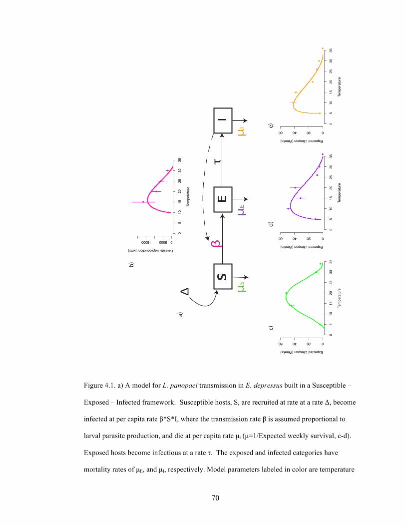
70

Figure 4.1. a) A model for L. panopaei transmission in E. depressus built in a Susceptible –

Exposed – Infected framework. Susceptible hosts, S, are recruited at rate at a rate Δ, become

infected at per capita rate β*S*I, where the transmission rate β is assumed proportional to

larval parasite production, and die at per capita rate µs (µ=1/Expected weekly survival, c-d).

Exposed hosts become infectious at a rate τ. The exposed and infected categories have

mortality rates of µE, and µI, respectively. Model parameters labeled in color are temperature

SI

E

∆ μS

τβ

μE

μI

b)

c)e)

d)

a)

●

●

●

●

●

Tem

pera

ture

Parasite Reproduction (lxmx)

05

1015

2025

3035

0500015000

●

●

●

●

●●

●

Tem

pera

ture

Expected Lifespan (Weeks)

05

1015

2025

3035

0204060

●

●●

●

●●

●

Tem

pera

ture

Expected Lifespan (Weeks)

05

1015

2025

3035

0204060

●

●

●

●

●

Tem

pera

ture

Expected Lifespan (Weeks)

05

1015

2025

3035

0204060

71

dependent, and are parameterized based thermal performance curves fit to experimental

measurements of survival and parasite reproduction. b) Thermal performance curves for

parasite transmission and c-e) survival across multiple stages of infection including c)

susceptible, d) exposed and e) infected hosts. The shape of parasite transmission in response

to temperature was estimated from the sum of age specific parasite larval production

calculated from 200 days of parasite reproduction (details in SOM). Expected weekly

survival was calculated from Kaplein-Meier survival curves with estimate of survival at each

temperature (details in SOM).

We investigated the ecological consequences of seasonal mismatch in thermal

performance for host and parasite by developing a compartmental model of host infection

(Anderson and May 1982), where parasite transmission and host survival are temperature

dependent (Figure 4.1). To describe the thermal environment of our host and parasite we

calculated mean weekly temperatures from a Georgia Coastal Ecosystems (GCE) buoy

that measured temperature at a depth of ~1m (Figure 4.2A), the approximate depth of

water found over an oyster reef in Georgia (Di Iorio 2012, 2013, 2014a, 2014b, Byers et

al. 2015), and thus the thermal environment experienced by E. depressus and L.

panopaei. The model dynamics rapidly converged on an annual seasonally-influenced

cycle of parasite prevalence (Figure 4.2D). Consistent with field observations

(O'Shaughnessy et al. 2014b), the model predicted that parasite prevalence would

increase in the winter, and decrease in spring and early summer (Figure 4.2D). The drop

in prevalence in the summer is driven by a combination of decreased parasite

transmission (Figure 4.2G) and greater infected host mortality (Figure 4.2J) with

increasing temperature (Figure 4.2A).

72

Figure 4.2. A: Temperatures used to drive seasonality in the host-parasite model, with the mean

water temperature from the Georgia Coastal Ecosystem Long Term Ecological Research station

10 averaged weekly from 2011 to 2014 B: mean +1 (solid green), mean +2 (solid purple), mean

+3 (solid light blue). C: Temperature increased based on hindcast from actual temperature change

in the southeast from 1970-2008 (Karl et al. 2009), with the mean +1.6 (solid blue) and

Tem

pera

ture

(ºC)

010

2030

40

Jan Mar May July Sept Nov

A

010

2030

40

Jan Mar May July Sept Nov

B

010

2030

40

Jan Mar May July Sept Nov

C

Prev

alen

ce

025

5075

100

Jan Mar May July Sept Nov

D

025

5075

100

Jan Mar May July Sept Nov

E

025

5075

100

Jan Mar May July Sept Nov

F

Para

site

Tran

smiss

ion

0.00

000

0.00

006

0.00

012

Jan Mar May July Sept Nov

G0.

0000

00.

0000

60.

0001

2

Jan Mar May July Sept Nov

H

0.00

000

0.00

006

0.00

012

Jan Mar May July Sept Nov

I

Infe

cted

Mor

tality

04

8

Jan Mar May July Sept Nov

J

04

8

Jan Mar May July Sept Nov

K

04

8

Jan Mar May July Sept Nov

L

Expo

sed

Mor

tality

04

8

Jan Mar May July Sept Nov

M

04

8

Jan Mar May July Sept Nov

N

04

8

Jan Mar May July Sept Nov

O

Susc

eptib

le M

orta

lity

04

8

Jan Mar May July Sept NovDate

P

04

8

Jan Mar May July Sept NovDate

Q

04

8

Jan Mar May July Sept NovDate

R

73

seasonally varying increases. D-F: Model predictions of seasonal prevalence. Temperature

dependant model parameters, including parasite transmission, β (G-I), infected host mortality (J-

L), exposed host mortality (M-O) and susceptible host mortality (P-R).

Model exploration showed that parameters were behaving in a biologically

realistic manner. We evaluated the minimum number of infected individuals within a

single year and found that infection was maintained by >1 infected or exposed individual

at all times throughout the season. To evaluate how robust the prediction of seasonality

was to a range of parameters values, we conducted sensitivity analyses (SOM).

Sensitivity analysis revealed that peak and mean prevalence, but not minimum

prevalence, increase with transmission rate, β (Figure S4.10), and only weakly depend on

the seasonal pattern of host recruitment, Δ (Figure S4.11) and latent period, τ (Figure

S4.13). The seasonal pattern of prevalence is robust to variation in parameter values, and

the timing of the seasonal peak in prevalence is most strongly influenced the timing of

the host recruitment peak (Figure S4.11).

To evaluate potential effects of climate change on host-parasite interactions in

ectothermic hosts, we ran model simulations at a range of increasing temperatures, from

the GCE mean +1, +2 and +3ºC (Christensen et al. 2007). We began each simulation

with infection prevalence around 30%, giving the parasite the best possible chance to

maintain infection through the season. Host-parasite cycling persisted with decreasing

amplitude in the model at +1 and +2º C (Figure 4.3N), and the parasite was driven out of

the system within a single season at mean +3ºC (Figure 4.3N). As we started the model

with higher prevalence than is predicted under current scenarios (or observed in the field,

(O'Shaughnessy et al. 2014a)), the estimate of parasite local extinction with a mean

increase of +3 ºC are conservative. Parasite extirpation is driven by warming induced

74

exacerbation of the seasonal drop in prevalence, specifically by greater infected host

mortality (Figure 4.2K) and decreased parasite transmission (Figure 4.2H).

In the Southeastern US, the increase in temperature as a result of climate change

in more intense in the winter months (Karl et al. 2009), and is not expected to increase

evenly across seasons in the future (Christensen et al. 2007). Thus, to explore the effects

of seasonally varying temperature, we used a simple hindcast of actual change in

temperature in the southeast from 1970-2008. We compared the effects of actual mean

temperature change and seasonally dependent temperature change (Figure 4.2C) on host-

parasite dynamics (details in SOM; (Karl et al. 2009). The model predicted slightly

higher maximum infection prevalence (+5%) and slight offsets in seasonality with

seasonally dependant temperature change (Figure 4.3O).

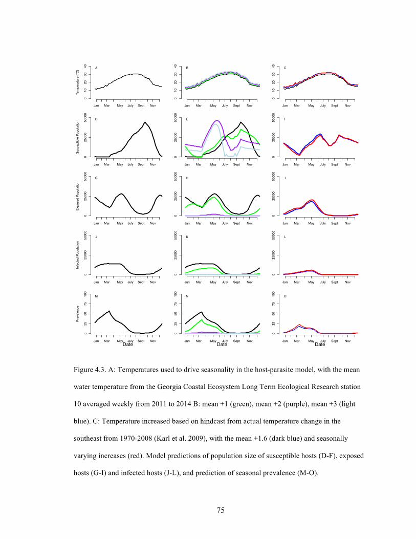
75

Figure 4.3. A: Temperatures used to drive seasonality in the host-parasite model, with the mean

water temperature from the Georgia Coastal Ecosystem Long Term Ecological Research station

10 averaged weekly from 2011 to 2014 B: mean +1 (green), mean +2 (purple), mean +3 (light

blue). C: Temperature increased based on hindcast from actual temperature change in the

southeast from 1970-2008 (Karl et al. 2009), with the mean +1.6 (dark blue) and seasonally

varying increases (red). Model predictions of population size of susceptible hosts (D-F), exposed

hosts (G-I) and infected hosts (J-L), and prediction of seasonal prevalence (M-O).

Tem

pera

ture

(ºC)

010

2030

40

Jan Mar May July Sept Nov

A

010

2030

40

Jan Mar May July Sept Nov

B

010

2030

40

Jan Mar May July Sept Nov

C

Susc

eptib

le P

opul

atio

n

025

000

5000

0

Jan Mar May July Sept Nov

D

025

000

5000

0

Jan Mar May July Sept Nov

E

025

000

5000

0

Jan Mar May July Sept Nov

F

Expo

sed

Popu

latio

n

025

000

5000

0

Jan Mar May July Sept Nov

G0

2500

050

000

Jan Mar May July Sept Nov

H

025

000

5000

0

Jan Mar May July Sept Nov

I

Infe

cted

Pop

ulat

ion

025

000

5000

0

Jan Mar May July Sept Nov

J

025

000

5000

0

Jan Mar May July Sept Nov

K

025

000

5000

0

Jan Mar May July Sept Nov

L

Prev

alen

ce

025

5075

100

Jan Mar May July Sept Nov

M

Date

025

5075

100

Jan Mar May July Sept Nov

N

Date

025

5075

100

Jan Mar May July Sept Nov

O

Date

76

This work highlights the consequences of parasite driven changes to host thermal

performance for parasite persistence. If this thermal mismatch in survival between

uninfected and infected hosts represents a general ectothermic host-parasite response,

then increasing temperature may accelerate the population decline of parasites, leading to

unexpected biodiversity loss. The differential in uninfected and infected host thermal

performance, particularly of survival, may have been missed in other studies that focused

on temperature effects on parasite transmission traits (Anderson and May 1979), such as

reproduction and infection probability (Morley and Lewis 2014, Paull et al. 2015), or

focused on survival of uninfected hosts only (Mordecai et al. 2013, Johnson et al. 2015).

There is a suggestion of generality from trematode systems – where there is a consistent

negative relationship between infected host mortality and temperature across a range of

temperatures likely within the thermal optima of the host (Paull et al. 2015). Even if the

thermal performance mismatch is not a generalized response, the inclusion of the non-

linear effect of temperature on parasites will likely increase the accuracy of predictions of

host-parasite interactions at higher temperatures (Mordecai et al. 2013). Non-linearity of

response can account for the preponderance of studies suggesting an increase in disease

transmission if those studies have been conducted in areas where measurements were

taken only on the rising side of the non-linear response (Figure 4.2). Indeed, in this study

if we were to only analyze the relationship between infection prevalence and temperature

from January-March we would assume a positive effect of temperature on transmission

(Figure 4.2).

The prediction that increased temperature could drive down disease can be

beneficial – for example, in temperate climates increased temperature increases the

77

spread of mosquito borne disease, such as malaria, but in hotter areas of the tropics there

may see a decrease in disease with increasing temperature (Mordecai et al. 2013). On the

other hand, parasites are also important members of communities and an influential

aspect of biodiversity, and their removal can have unintended (and often undetected)

consequences on the predators or prey of their hosts (Wood and Johnson 2015). Parasites

can alter host dynamics (Figure S7, (Hudson and Greenman 1998)), are themselves prey

(Kaplan et al. 2009), and can enhance transfer of energy to higher trophic levels through

manipulation of their hosts (Lafferty and Morris 1996). In fact, predation rates on L.

panopaei infected E. depressus are three times that of uninfected hosts, suggesting that

removal of this parasite from the system will alter prey availability (Gehman and Byers,

in review). Our model results corroborate recent regional scale observations from the

field that demonstrate that prevalence is limited in its southern range (e.g. absent in

southern Florida), and early indication that the parasite may be expanding its range

further north up the Atlantic coast of the US.

In sum, this work reveals a thermal mismatch in performance between uninfected

and infected hosts that leads to the prediction of local extirpation of the parasite under

moderate climate change scenarios. If the thermal mismatch found here can be

generalized for ectothermic host-parasite interactions at high temperature, then this may

cause hitherto unforeseen emergent effects on community and ecosystem dynamics.

78

Supplemental Online Material

Methods

System and Field Collection

Host Natural History

Eurypanopeus depressus is an abundant oyster reef-dwelling crab occurring from

the Gulf of Mexico to Massachusetts Bay. Temperature varies considerably across this

range, and within individual sites seasonally. As an ecotherm, E. depressus body

temperature can be expected to conform to the surrounding water temperature (Willmer,

Stone and Johnson text). Refuge within the oyster reef ameliorates desiccation stress and

protects them from predation (Grant and McDonald 1979, Hulathduwa et al. 2007).

While there is a great range of oyster reef size and shape, the average reef found in

Chatham County, GA is ~200m2 (Corely and Harris, Harris personal communication).

Average density of E. depressus is 120 adult m-2 (4-20mm carapace width) and 140

juvenile m-2 (<4mm carapace width, Gehman et. al. in review).

The mean expected longevity of adult E. depressus (from their first larval release)

is 2.2 year, with a maximum life span of 3.5 years (McDonald 1982). Female E.

depressus in South Carolina have two broods per year, with two peaks of ovigerous

reproduction, with the first peak in April-May and the second peak late August-

September, however ovigerous females can be found any time between March and

October (McDonald 1982). Interestingly, larval recruitment is year-round in south

Florida, but had similar peaks late spring and summer (Tolley et al. 2006), with decreased

reproduction correlated with decreased salinity associated with the wet season (Miner et

al. 2013). Further north recruitment seems to come in a single pulse, from July to

79

October (although this study measured all xanthid recruitment and only collected in the

spring for a single year;(Jones and Epifanio 1995)). Eurypanopeus depressus has 4 zoeal

stages and one megalopal stage (under laboratory conditions; (Costlow and Bookhout

1961). Larval behavior suggests that E. depressus recruitment is retained within estuaries,

with larvae migrating towards the surface during flood tide and towards the bottom at ebb

tide (Sulkin 1984, Epifanio and Tilburg 2008). While recruitment is likely relatively

closed within an estuary, reefs within the estuary are likely experiencing open

recruitment from within the estuary.

Parasite Natural History

Loxothylacus panopaei is a castrating rhizocephalan barnacle parasite that infects

the mud crab Eurypanopeus depressus, as well as several other mud crabs (Reinhard and

Reischman 1958; Kruse et al. 2011). Loxothylacus panopaei is native to the Gulf of

Mexico and introduced to the US Atlantic coast from Long Island, New York to Cape

Canaveral, Florida. Genetic work suggests that there are three lineages of this parasite,

and only the ER lineage is invasive along the US Atlantic coast (Kruse et al. 2011).

Eurypanopeus depressus is infected by the ER lineage, which was first documented in

North Carolina in 1983 and in Georgia and northeastern Florida in 2004/2005 (Kruse and

Hare 2007; Eash-Loucks et al. 2014). The Harris mud crab Rithropanopeus harrisi is

also infected by the ER lineage, and could serve as a resevoir host for this parasite,

however it is generally found in lower salinities and has not been document near where

this study took place (Prezant et al. 2002)(personal observation). While L. panopaei is

present within the Gulf of Mexico and in Northern Florida, it has not been reported in

Southeastern Florida, suggesting that the higher temperatures in Southeastern Florida

80

may represent poor conditions for the parasite and be limiting spread (Kruse et al. 2011).

At a local level, there is evidence that temperature may drive seasonal patterns in parasite

infection, with infection prevalence increasing in the spring, followed by a marked

decrease in infection prevalence mid-summer, correlated with temperatures reaching

above 25° C (O'Shaughnessy et al. 2014b). Together these observations suggest that

temperature may be driving changes L. panopaei infection prevalence.

Rhizocephalans have direct transmission, and the adult parasite resides within its

crab host and produces larvae, lending itself for quantification of reproductive output.

Loxothylacus panopaei larvae are planktonic and lecithotrophic (non-feeding), take 2-5

days to become infectious and can be male or female (Walker et al. 1992, Walker 2001).

Larval sex dictates it’s role within the transmission cycle; female larvae find and infect

susceptible hosts, form an internal infection (interna) and then release a virgin externa

(Glenner 2001). Exposed hosts are infected, but non-reproductive and the time to release

of the virgin externa can take from 18-57 days (Alvarez et al. 1995). For the parasite to

become reproductive, and thus infectious, a male larvae (or two) must recruit to the virgin

externa after which the ovary develops to reproductive maturity (Hoeg 1995). The time

between male larval colonization of an exposed host and reaching parasite reproductive

maturity can take from 18-22 days (Alvarez et al. 1995).

Collection

To create thermal performance curves for multiple stages of parasite infection, we

collected crabs from a single location from Romerly Marsh Creek, Savannah, GA

(31°55'15.5"N 80°59'13.0"W) from 9th March to 23rd April, 2014. We collected a single

cohort of infected individuals to standardize infection age, as age of infection may

81

determine parasite reproduction. Previous observation by A. Gehman suggested that in

Georgia there is semi-synchronized release of virgin externa correlated with the seasonal

increase in ambient water temperature above ~20°C (personal observation). To collect a

cohort of approximately the same age L. panopaei infections, we isolated crabs not

exhibiting external infections, held them at ambient temperature, fed them ad libidum

with frozen brine shrimp and monitored for evidence of externa release. New infections

were first noted 24th April 2014, and we began the experiment on May 13th,; thus

infections used for the experiment were all less then a month old when the experiment

began.

Internal infection is highly prevalent in the spring months, an ideal time for

collecting multiple stages of parasite infection, however for that reason it was also a very

difficult time to collect uninfected crabs. Additionally, as noted above, the lack of

manifested externa does not guarantee that crabs are uninfected. Loxothylacus panopaei

causes complete sterilization, so if a female is ovigerous then it is not currently infected

(Alvarez et al. 1995, Hoeg 1995). In addition, L. panopaei feminizes its host, so E.

depressus that have strong morphologically male characteristics are less likely to be

infected. To take advantage of these traits and increase the chances of collecting

uninfected hosts, we collected ovigerous females and male E. depressus. For the

logistical reasons described above, the uninfected E. depressus collection began a few

months after the start of the infected crab experiment. Collection was conducted from the

3rd of July and the 4th of September 2014, and collected crabs were maintained filtered

seawater in individual jars at ambient temperature and monitored for any evidence of

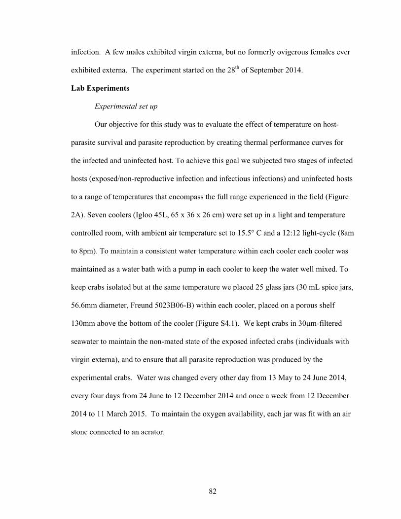
82

infection. A few males exhibited virgin externa, but no formerly ovigerous females ever

exhibited externa. The experiment started on the 28th of September 2014.

Lab Experiments

Experimental set up

Our objective for this study was to evaluate the effect of temperature on host-

parasite survival and parasite reproduction by creating thermal performance curves for

the infected and uninfected host. To achieve this goal we subjected two stages of infected

hosts (exposed/non-reproductive infection and infectious infections) and uninfected hosts

to a range of temperatures that encompass the full range experienced in the field (Figure

2A). Seven coolers (Igloo 45L, 65 x 36 x 26 cm) were set up in a light and temperature

controlled room, with ambient air temperature set to 15.5° C and a 12:12 light-cycle (8am

to 8pm). To maintain a consistent water temperature within each cooler each cooler was

maintained as a water bath with a pump in each cooler to keep the water well mixed. To

keep crabs isolated but at the same temperature we placed 25 glass jars (30 mL spice jars,

56.6mm diameter, Freund 5023B06-B) within each cooler, placed on a porous shelf

130mm above the bottom of the cooler (Figure S4.1). We kept crabs in 30µm-filtered

seawater to maintain the non-mated state of the exposed infected crabs (individuals with

virgin externa), and to ensure that all parasite reproduction was produced by the

experimental crabs. Water was changed every other day from 13 May to 24 June 2014,

every four days from 24 June to 12 December 2014 and once a week from 12 December

2014 to 11 March 2015. To maintain the oxygen availability, each jar was fit with an air

stone connected to an aerator.

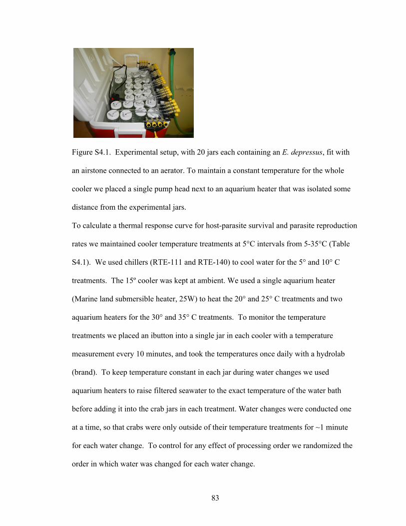
83

Figure S4.1. Experimental setup, with 20 jars each containing an E. depressus, fit with

an airstone connected to an aerator. To maintain a constant temperature for the whole

cooler we placed a single pump head next to an aquarium heater that was isolated some

distance from the experimental jars.

To calculate a thermal response curve for host-parasite survival and parasite reproduction

rates we maintained cooler temperature treatments at 5°C intervals from 5-35°C (Table

S4.1). We used chillers (RTE-111 and RTE-140) to cool water for the 5° and 10° C

treatments. The 15º cooler was kept at ambient. We used a single aquarium heater

(Marine land submersible heater, 25W) to heat the 20° and 25° C treatments and two

aquarium heaters for the 30° and 35° C treatments. To monitor the temperature

treatments we placed an ibutton into a single jar in each cooler with a temperature

measurement every 10 minutes, and took the temperatures once daily with a hydrolab

(brand). To keep temperature constant in each jar during water changes we used

aquarium heaters to raise filtered seawater to the exact temperature of the water bath

before adding it into the crab jars in each treatment. Water changes were conducted one

at a time, so that crabs were only outside of their temperature treatments for ~1 minute

for each water change. To control for any effect of processing order we randomized the

order in which water was changed for each water change.

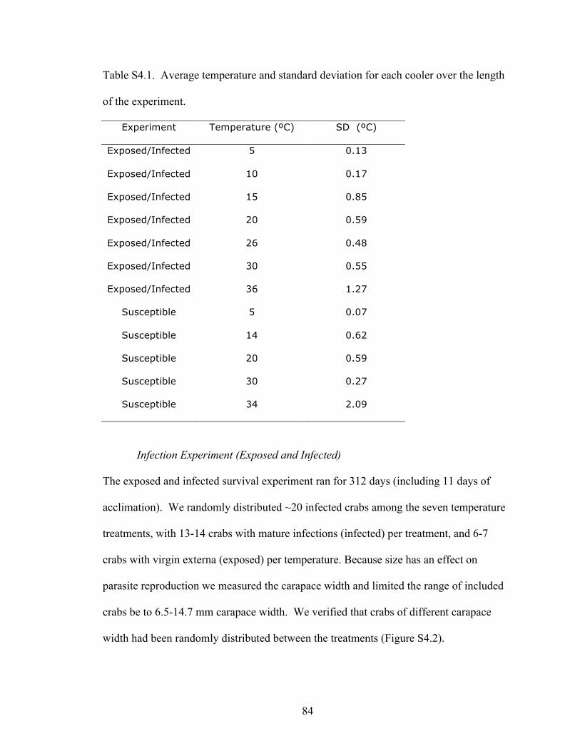
84

Table S4.1. Average temperature and standard deviation for each cooler over the length

of the experiment.

Experiment Temperature (ºC) SD (ºC)

Exposed/Infected 5 0.13

Exposed/Infected 10 0.17

Exposed/Infected 15 0.85

Exposed/Infected 20 0.59

Exposed/Infected 26 0.48

Exposed/Infected 30 0.55

Exposed/Infected 36 1.27

Susceptible 5 0.07

Susceptible 14 0.62

Susceptible 20 0.59

Susceptible 30 0.27

Susceptible 34 2.09

Infection Experiment (Exposed and Infected)

The exposed and infected survival experiment ran for 312 days (including 11 days of

acclimation). We randomly distributed ~20 infected crabs among the seven temperature

treatments, with 13-14 crabs with mature infections (infected) per treatment, and 6-7

crabs with virgin externa (exposed) per temperature. Because size has an effect on

parasite reproduction we measured the carapace width and limited the range of included

crabs be to 6.5-14.7 mm carapace width. We verified that crabs of different carapace

width had been randomly distributed between the treatments (Figure S4.2).

85

Figure S4.2. The mean and SD of host size for each of the temperature treatments.

The ambient temperature at the beginning of the experiment was ~20º C and we started

all temperature treatments at that temperature. We acclimated the E. depressus to their

experimental treatments over the following 10 days, adjusting cooler temperatures by

2°C per day. The 2ºC temperature change was gradual, as we changed the setting of the

water bath and let the bath slowly increase to the new temperature. Water changes were

conducted throughout the acclimation period, however we only analyze results starting

after this transition period when the crabs had been at experimental temperature for a full

day (day 11, May 25th 2014).

We monitored crabs at each water change. At each monitoring we checked for crab and

parasite mortality and parasite larval release. Nauplii and cyprids are visible to the naked

eye, and we tested our detection limit and found that we could correctly identify empty

jars. In a dilution detection test we detected nauplii down to ~5 nauplii per jar. We

changed the water and fed the E. depressus the equivalent of one brine shrimp per day. In

jars where we detected a release, or we were not confident of lack of release, we collected

all larvae released by pouring out the water through a 30 µm mesh, then refilling the jar

and again filtering the water through the mesh. Crabs remained within their jars

throughout water changes. We then rinsed the contents on the mesh into a scintillation

vial with ~15mL of 90% ethanol and stored for later quantification.

●●

● ●●

● ●

0 10 20 30 40

46

810

1214

Temperature (ºC)

Hos

t Size

(mm

)

86

We quantified the number of larvae released using a 1mm3 gridded sedgewick rafter slide

(model# 1801-G20). We homogenized samples, collected 1mL of sample and placed it

into the counting chamber. We quantified all larvae present (cyprids, nauplii and eggs).

We quantified the remaining volume of the sample in a graduated cylinder. Total number

of larvae released was calculated by multiplying the number of larvae calculated in 1µL

by the total volume of the sample.

Uninfected Experiment (Susceptible)

Because of limitations (difficulty) in the collection of uninfected crabs we used fewer

temperature treatments, but still captured the limits of the thermal curve (Table S4.1). An

additional five coolers were set up to run the uninfected E. depressus experiment. Crabs

were acclimated as described above, except that ambient water temperature was closer to

25ºC, and acclimation was done from that temperature. At each monitoring point we

checked for crab mortality and any evidence of infection. We did not find evidence of

infection for any individual included in the susceptible category. The uninfected –

susceptible- experiment ran for 169 days (including 11 days of acclimation time).

Analysis

To get estimates of the effect of temperature on survival for each of the treatments

we conducted survival analysis across temperature for the uninfected (susceptible),

exposed (virgin externa) and infected E. depressus. We evaluated each infection status

category individually using Kaplan-Meier survival analysis with the R package survival.

This and all subsequent analyses and simulations were conducted using R (R

Development Core Team 2015). We calculated the restricted mean survival time (RMST)

at each temperature, which allowed us to estimate the expected weekly survival across

87

treatments, even if experiments were not run for an equal length (Royston and Parmar

2011)(Hosmer and Lemeshow, pg. 53:57). Additionally RMST does not require

proportional response of all treatments to temperature and can accommodate censored

data – e.g. crabs that hadn’t died by the end of the experiment or were removed for other

reasons besides mortality (Hosmer and Lemeshow). We calculated RMST by estimating

the area under the curve up to time t*, which we set to 365 days, which allowed us

evaluate the expected number of weeks each infection category would be expected to

experience out of a year.

To evaluate the shape of the effect of temperature on host and parasite

performance traits we fit functions relating performance to temperature. We fit three

functions to evaluate whether the relationship was quadratic (symmetrical) or left or right

skewed in response to temperature. The Briere function can capture the non-linear effects

of temperature on ectotherm performance however it is limited to the right-skewed

patterns often evident in ectotherm response to temperature (Briere et al. 1999). To

evaluate whether responses were right- or left-skewed, we flipped and reversed the Briere

to create a modified Briere function that could fit a left-skewed pattern. We evaluated

whether there was any evidence for either skew using a quadratic function. To evaluate

the best fit for temperature dependence for each variable we fit a quadratic, Briere and a

modified Briere function to each infection class. We evaluated model fit through AICc.

Model Development

We investigated the ecological consequences of the thermal performance mismatch for

host and parasite found in our experiments through a simple compartmental model. We

used this model to describe seasonal disease dynamics of an E. depressus population

88

within a single oyster reef. The host population was categorized according to L.

panopaei infection status, such that S represents the abundance of uninfected, susceptible

E. depressus, E represents the abundance of infected but non-reproductive E. depressus

(i.e. individuals with internal infections or virgin externa) and I represents infectious E.

depressus (i.e. those with externa producing parasite larvae). Pelagic free-living infective

stages of female and male parasite larvae are denoted by Wf and Wm respectively.

In the absence of the parasite, the crab population experiences recruitment at a rate Δ and

per capita mortality at a rate µS. When the parasite is introduced into the system,

susceptible hosts are infected at a per capita rate that is a function of the abundance of

free-living female larvae (Wf). Exposed hosts die at rate µE and move to the infectious

class depending on time to development of a virgin externa (1/τ) and the probability of

encountering male larvae, πWm. Infectious individuals die at rate µI , and release infected

female and male larvae at respective rates λf and λm. Pelagic larval mortality is

considered equal (and high) for both sexes and occurs at rate µw. Therefore parasite

transmission can be described by the following system of equations:

Eq 1

Eq 2

Eq 3

Eq 4

89

Eq 5

Female larvae must find a host, evade the host immune system and form an interna,

whereas male larvae are left with the relatively simple task of fertilizing an infected host

(which is presumably attempting to attract a mate). As such, we assumed that male larvae

were not the limiting factor for transmission, and if a female larva infects a susceptible

host and moves into the exposed category, a male larva will fertilize it. Through this

assumption we restrict the temperature limitation on the parasite to the female

colonization rate – so that if the temperature is such that female larvae are being

produced and colonizing then we assume that temperature will be acceptable for the male

larvae colonization and externa development.

We make the following (plausible) simplifying assumptions to reduce model complexity

and better match experimental data:

Since larval parasite mortality is high relative to host mortality (i.e. µw >> µs), we can

make a the following quasi-equilibrium approximation:

Eq 6

If we further assume that host infection rate scales linearly with larval parasite density,

the transmission rate can we expressed as βSI, where the transmission rate β, is the

product of the contact rate C, the probability of infection given contact (πf), and the

number of female larvae produced by one infectious host during the expected lifespan of

a larva ( ) :

90

Eq 7

Finally, as there are many more limiting steps for female infection, including evading the

host immune system and developing the interna (Hoeg 1995), we assume that male

parasite larvae are never limiting relative to the abundance of female larvae, so that all

virgin externa are fertilized with probability πmWm=1.

Under these assumptions, the model simplifies to:

Eq 8

Eq 9

Eq 10

Parameterization

To explore how temperature affects host-parasite interactions we allowed several

model parameters to vary with temperature, including mortality rates for susceptible (S),

exposed (E) and infected (I) host and parasite reproduction rate (β). To parameterize

temperature dependence for the mortality of each class and parasite reproduction we

incorporate the thermal performance curves created in the laboratory experiments.

Mortality rate, µ is estimated by the inverse of the expected weekly survival calculated

above, and through the use of functional fits to the survival data we are able to let µ vary

dependent on temperature (Figure 4.2). Similarly, the reproduction rate β is set by the

reproductive output calculated above and varies with temperature (Figure 4.2).

91

The remaining model parameters were set based on previous literature (Gehman et al;

(Alvarez et al. 1995)) and are described in Table S4.2. While not strictly temperature

dependent, we accounted for seasonality (and likely temperature dependence) of host

reproduction by limiting recruitment to March-October. Host recruitment rate was set

based on the number of juveniles found m-2 in a survey conducted in 2010 (Gehman et al.

in review). While it seems probable that τ, development from exposed to infectious is

also temperature dependent; there is no evidence to support this relationship either in the

literature or from our experiments. The reported variance in time from exposed to

infectious is relatively short (18-22 days), and the time to development is shorter than

transitions in the model, so we chose a constant τ across temperature.

Table S4.2. Description of the parameters used for the model.

Term Definition Dependence

Support Units Estimate

Δ Hostrecruitment Seasonal

Estimatedfromliterature

(Gehmanetal)

Numberofjuvenilerecruits

5000

μs Susceptiblemortality

Temperature Fig.1 Weekly

mortalityBriereFunction

βTransmission(susceptibletoexposed)

Temperature Fig.1

#oflarvaeproduced

ModifiedBriereFunction

τ

Parasitedevelopment(exposedtoinfected)

Constant

Estimatedfromliterature

(Alvarezetal.1995)

Weekly

0.05

μE Exposedhostmortality

Temperature Fig.1

Weeklymortality

ModifiedBriereFunction

μI Infectedhostmortality

Temperature Fig.1

Weeklymortality

ModifiedBriereFunction

Sensitivity Analysis

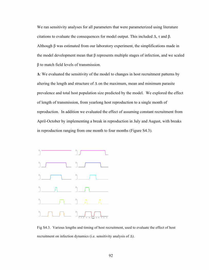
92

We ran sensitivity analyses for all parameters that were parameterized using literature

citations to evaluate the consequences for model output. This included Δ, τ and β.

Although β was estimated from our laboratory experiment, the simplifications made in

the model development mean that β represents multiple stages of infection, and we scaled

β to match field levels of transmission.

Δ: We evaluated the sensitivity of the model to changes in host recruitment patterns by

altering the length and structure of Δ on the maximum, mean and minimum parasite

prevalence and total host population size predicted by the model. We explored the effect

of length of transmission, from yearlong host reproduction to a single month of

reproduction. In addition we evaluated the effect of assuming constant recruitment from

April-October by implementing a break in reproduction in July and August, with breaks

in reproduction ranging from one month to four months (Figure S4.3).

Fig S4.3. Various lengths and timing of host recruitment, used to evaluate the effect of host

recruitment on infection dynamics (i.e. sensitivity analysis of Δ).

05000

05000

05000

05000

05000

05000

05000

05000

05000

05000

05000

05000

Jan Feb Mar Apr May June July Aug Sept Oct Nov DecDate

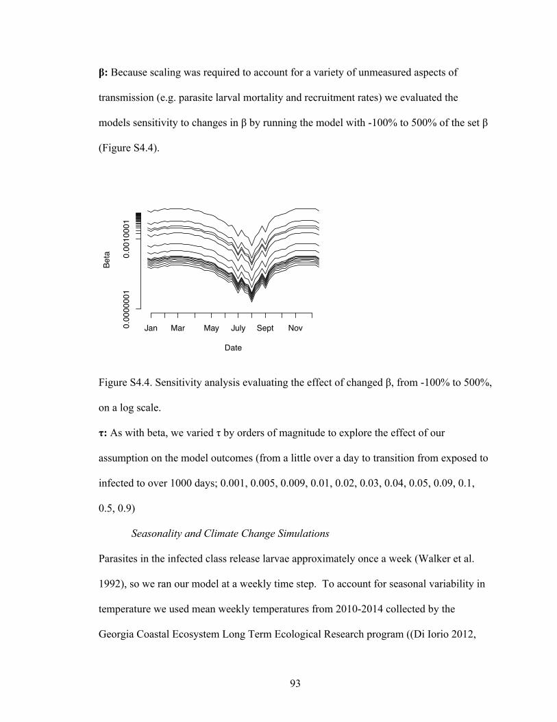
93

β: Because scaling was required to account for a variety of unmeasured aspects of

transmission (e.g. parasite larval mortality and recruitment rates) we evaluated the

models sensitivity to changes in β by running the model with -100% to 500% of the set β

(Figure S4.4).

Figure S4.4. Sensitivity analysis evaluating the effect of changed β, from -100% to 500%,

on a log scale.

τ: As with beta, we varied τ by orders of magnitude to explore the effect of our

assumption on the model outcomes (from a little over a day to transition from exposed to

infected to over 1000 days; 0.001, 0.005, 0.009, 0.01, 0.02, 0.03, 0.04, 0.05, 0.09, 0.1,

0.5, 0.9)

Seasonality and Climate Change Simulations

Parasites in the infected class release larvae approximately once a week (Walker et al.

1992), so we ran our model at a weekly time step. To account for seasonal variability in

temperature we used mean weekly temperatures from 2010-2014 collected by the

Georgia Coastal Ecosystem Long Term Ecological Research program ((Di Iorio 2012,

Date

Beta

0.0000001

0.0010001

Jan Mar May July Sept Nov

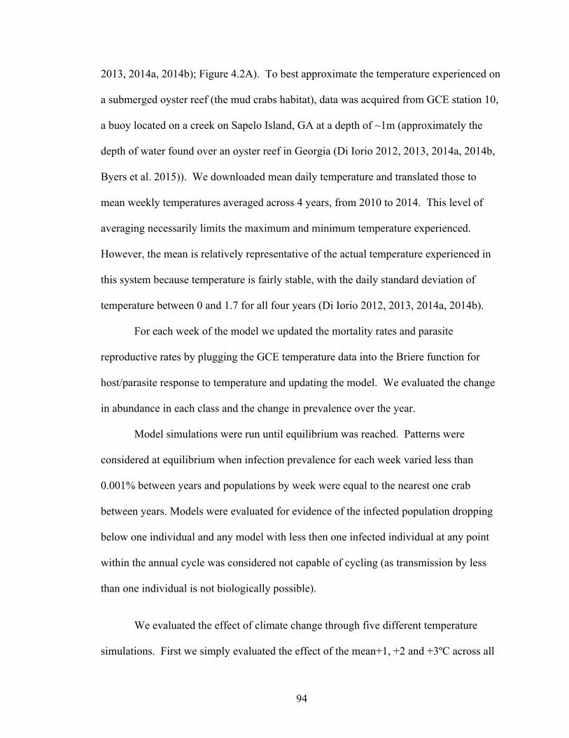
94

2013, 2014a, 2014b); Figure 4.2A). To best approximate the temperature experienced on

a submerged oyster reef (the mud crabs habitat), data was acquired from GCE station 10,

a buoy located on a creek on Sapelo Island, GA at a depth of ~1m (approximately the

depth of water found over an oyster reef in Georgia (Di Iorio 2012, 2013, 2014a, 2014b,

Byers et al. 2015)). We downloaded mean daily temperature and translated those to

mean weekly temperatures averaged across 4 years, from 2010 to 2014. This level of

averaging necessarily limits the maximum and minimum temperature experienced.

However, the mean is relatively representative of the actual temperature experienced in

this system because temperature is fairly stable, with the daily standard deviation of

temperature between 0 and 1.7 for all four years (Di Iorio 2012, 2013, 2014a, 2014b).

For each week of the model we updated the mortality rates and parasite

reproductive rates by plugging the GCE temperature data into the Briere function for

host/parasite response to temperature and updating the model. We evaluated the change

in abundance in each class and the change in prevalence over the year.

Model simulations were run until equilibrium was reached. Patterns were

considered at equilibrium when infection prevalence for each week varied less than

0.001% between years and populations by week were equal to the nearest one crab

between years. Models were evaluated for evidence of the infected population dropping

below one individual and any model with less then one infected individual at any point

within the annual cycle was considered not capable of cycling (as transmission by less

than one individual is not biologically possible).

We evaluated the effect of climate change through five different temperature

simulations. First we simply evaluated the effect of the mean+1, +2 and +3ºC across all

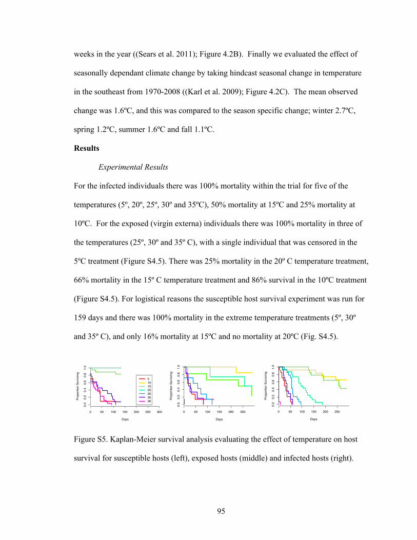
95

weeks in the year ((Sears et al. 2011); Figure 4.2B). Finally we evaluated the effect of

seasonally dependant climate change by taking hindcast seasonal change in temperature

in the southeast from 1970-2008 ((Karl et al. 2009); Figure 4.2C). The mean observed

change was 1.6ºC, and this was compared to the season specific change; winter 2.7ºC,

spring 1.2ºC, summer 1.6ºC and fall 1.1ºC.

Results

Experimental Results

For the infected individuals there was 100% mortality within the trial for five of the

temperatures (5º, 20º, 25º, 30º and 35ºC), 50% mortality at 15ºC and 25% mortality at

10ºC. For the exposed (virgin externa) individuals there was 100% mortality in three of

the temperatures (25º, 30º and 35º C), with a single individual that was censored in the

5ºC treatment (Figure S4.5). There was 25% mortality in the 20º C temperature treatment,

66% mortality in the 15º C temperature treatment and 86% survival in the 10ºC treatment

(Figure S4.5). For logistical reasons the susceptible host survival experiment was run for

159 days and there was 100% mortality in the extreme temperature treatments (5º, 30º

and 35º C), and only 16% mortality at 15ºC and no mortality at 20ºC (Fig. S4.5).

Figure S5. Kaplan-Meier survival analysis evaluating the effect of temperature on host

survival for susceptible hosts (left), exposed hosts (middle) and infected hosts (right).

Days

Prop

ortio

n Su

rviv

ing

5101520263036

0 50 100 150 200 250 300

0.0

0.2

0.4

0.6

0.8

1.0

Days

Prop

ortio

n Su

rviv

ing

0 50 100 150 200 250

0.0

0.2

0.4

0.6

0.8

1.0

Days

Prop

ortio

n Su

rviv

ing

0 50 100 150 200 250

0.0

0.2

0.4

0.6

0.8

1.0

96

Expected weekly survival (used in the model) was evaluated by calculating the area

under the curve for survival at each temperature.

Susceptible survival had a non-linear response to temperature and the best

described by a Briere Function (Figure 4.1b-e, Table S4.3). Exposed and infected

survival also had a non-linear response to temperature, however the best fitting function

was the modified Briere, accounting for the right-skew in the survival response (Figure

4.1c, Table S4.3). Parasite reproduction also varied non-linearly with temperature and

was best described by a modified Briere (Figure 4.1b, Table S4.3).

Table S4.3. The best fit function, the thermal minima (T0) and maxima (TM) and the

AIC for that function. For comparison the AIC score for the same data with the response

evaluated as a quadratic function of temperature is provided.

Infection

status Response Function T0 TM AIC Quad AIC

Susceptible Survival Briere 4.05 33.85 27.52 40.35

Exposed Survival Modified

Briere 4.81 34.63 52.73 61.92

Infected Survival Modified

Briere 4.99 31.9 44.8 61.92

Infected Reproduction Modified

Briere 9.87 30.75 98.29 104.09

Model Results:

Disease Free: The disease free model shows seasonality, driven by host recruitment and

host mortality rates (Figure S4.6). Comparison of host population between the disease-

97

free model and the model with infection reveals why pulsed reproduction is important for

consistency of model results found when varying Δ. It appears that without fall

recruitment the infection levels in the spring and early summer will drive the host

population to 0.

Figure S4.6. The susceptible (green) population over a single year in the model run

without disease (left). The susceptible, exposed (purple) and infected (orange)

populations over a single year in a model run to equilibrium with disease introduced in

the population.

Model Simulations:

Model simulations reached a repeating pattern of infection quickly, after 5 annual cycles

(Figure S4.7). The number of infected individuals increased with water temperature from

October through mid-May, followed by a decrease in infected individuals when

temperatures rise above ~25ºC (Fig. 4.3J). The number of exposed individuals has a

double peak through the season, with the second peak likely driven by the onset of

susceptible host recruitment in March (Fig. 4.3G and Fig. S4.12). Exposed individuals

also show a marked decrease in population size at temperatures above 25ºC, however the

040

000

8000

012

0000

Popu

latio

n Si

ze

Jan Mar May July Sept NovDate

040

000

8000

012

0000

Popu

latio

n Si

zeJan Mar May July Sept Nov

Date

98

trough of the response is higher, suggesting that exposed hosts are maintaining infection

in the population through the hot summer months (Fig. 4.3G).

Figure S4.7. Prevalence over years.

Climate Change

Model Sensitivity Results:

β: The model was sensitive to changes in β, particularly lowering of β (Figure S4.8 and

S4.9). With ~40% reduction in β the parasite fails to invade the population and infection

prevalence stays at 0%. However, even with a 300% increase in β there is only a slight

increase in the maximum and mean prevalence, and the result that high temperatures limit

reproduction in July and August remains robust to changes in β (Figure S4.8 and S4.9).

●●●●●●●●●●●●●●●●●●●●●●●●●●●●●●●●●●●●●●●●●●●●●●●●●●●●●●●●

●

●

●

●

●

●

●

●●●●●●●●●●●●

●

●●

●

●●●●●●●●●●●●●●●●●●●●

●

●

●

●

●

●

●

●

●

●

●

●●●●●●

●

●

●

●●●●●●●

●

●

●

●

●

●●●●●●●●●●●●●●●

●●●●●

●

●

●

●

●

●

●

●

●

●

●

●●●●●●

●

●

●

●●●●●●●

●

●

●

●

●

●●●●●●●●●●●●●●●

●●●●●

●

●

●

●

●

●

●

●

●

●

●

●●●●●●

●

●

●

●●●●●●●

●

●

●

●

●

●●●●●●●●●●●●●●●

●●●●●

●

●

●

●

●

●

●

●

●

●

●

●●●●●●

●

●

●

●●●●●●●

●

●

●

●

●

●●●●●●●●●●●●●●●

●●●●●

●

●

●

●

●

●

●

●

●

●

●

●●●●●●

●

●

●

●●●●●●●

●

●

●

●

●

●●●●●●●●●●●●●●●

●●●●●

●

●

●

●

●

●

●

●

●

●

●

●●●●●●

●

●

●

●●●●●●●

●

●

●

●

●

●●●●●●●●●●●●●●●

●●●●●

●

●

●

●

●

●

●

●

●

●

●

●●●●●●

●

●

●

●●●●●●●

●

●

●

●

●

●●●●●●●●●●●●●●●

●●●●●

●

●

●

●

●

●

●

●

●

●

●

●●●●●●

●

●

●

●●●●●●●

●

●

●

●

●

●●●●●●●●●●●●●●●

●●●●●

●

●

●

●

●

Years

Prevalence

1 2 3 4 5 6 7 8 9 10 11

010

2030

4050

60

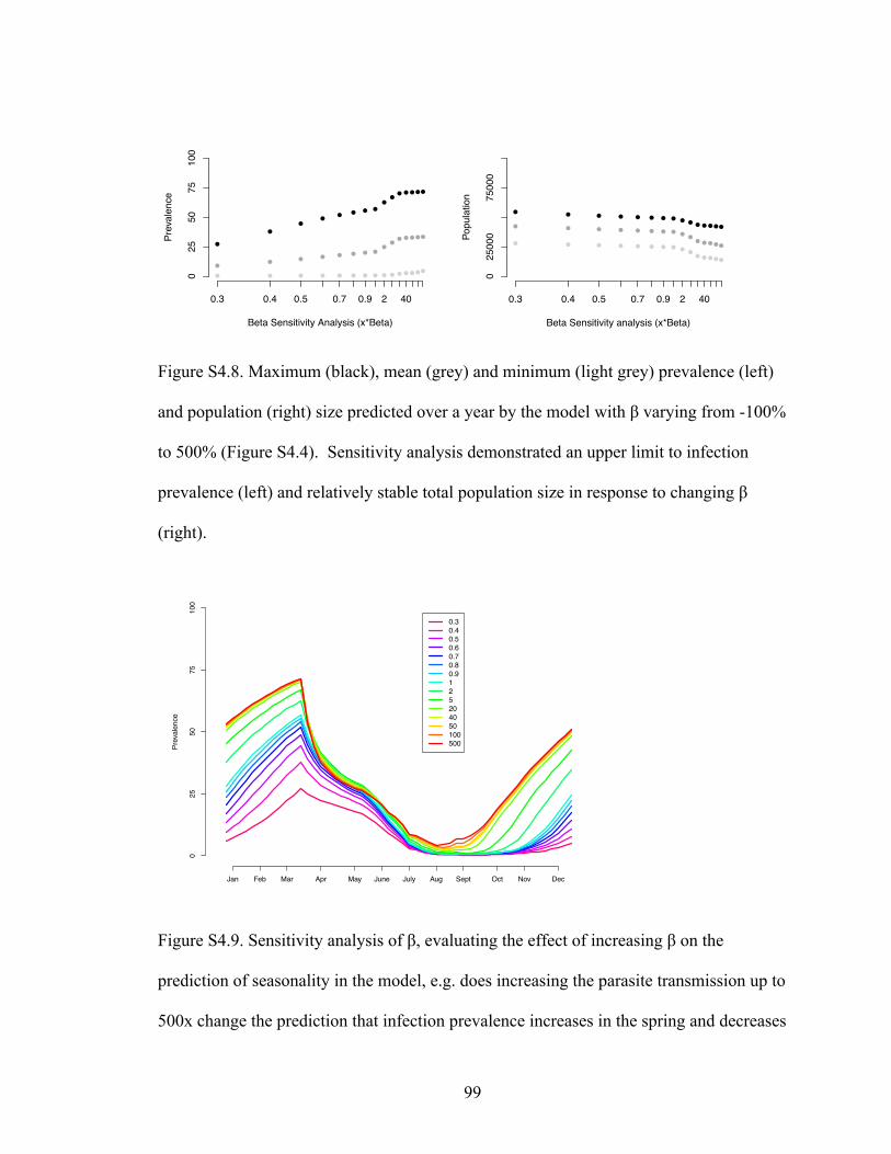
99

Figure S4.8. Maximum (black), mean (grey) and minimum (light grey) prevalence (left)

and population (right) size predicted over a year by the model with β varying from -100%

to 500% (Figure S4.4). Sensitivity analysis demonstrated an upper limit to infection

prevalence (left) and relatively stable total population size in response to changing β

(right).

Figure S4.9. Sensitivity analysis of β, evaluating the effect of increasing β on the

prediction of seasonality in the model, e.g. does increasing the parasite transmission up to

500x change the prediction that infection prevalence increases in the spring and decreases

Beta Sensitivity Analysis (x*Beta)

Prev

alen

ce

●

●

●

●

●

●

●

●

●

●

●

●

●

●

●

●

●

●

●

●

●

●

●

●

●

●

●

●

●

●

●

●

●

●

●

●

●

●

●

●

●

●

●

●

●

025

5075

100

0.3 0.4 0.5 0.7 0.9 2 40

Beta Sensitivity analysis (x*Beta)

Popu

latio

n

●

●

●

●

●

●

●

●

●

●

●

●

●

●

●

●

●

●

●

●

●

●

●

●

●

●

●

●

●

●

●

●

●

●

●

●

●

●

●

●

●

●

●

●

●

025

000

7500

0

0.3 0.4 0.5 0.7 0.9 2 40

Prevalence

025

5075

100

Jan Feb Mar Apr May June July Aug Sept Oct Nov Dec

0.30.40.50.60.70.80.9125204050100500

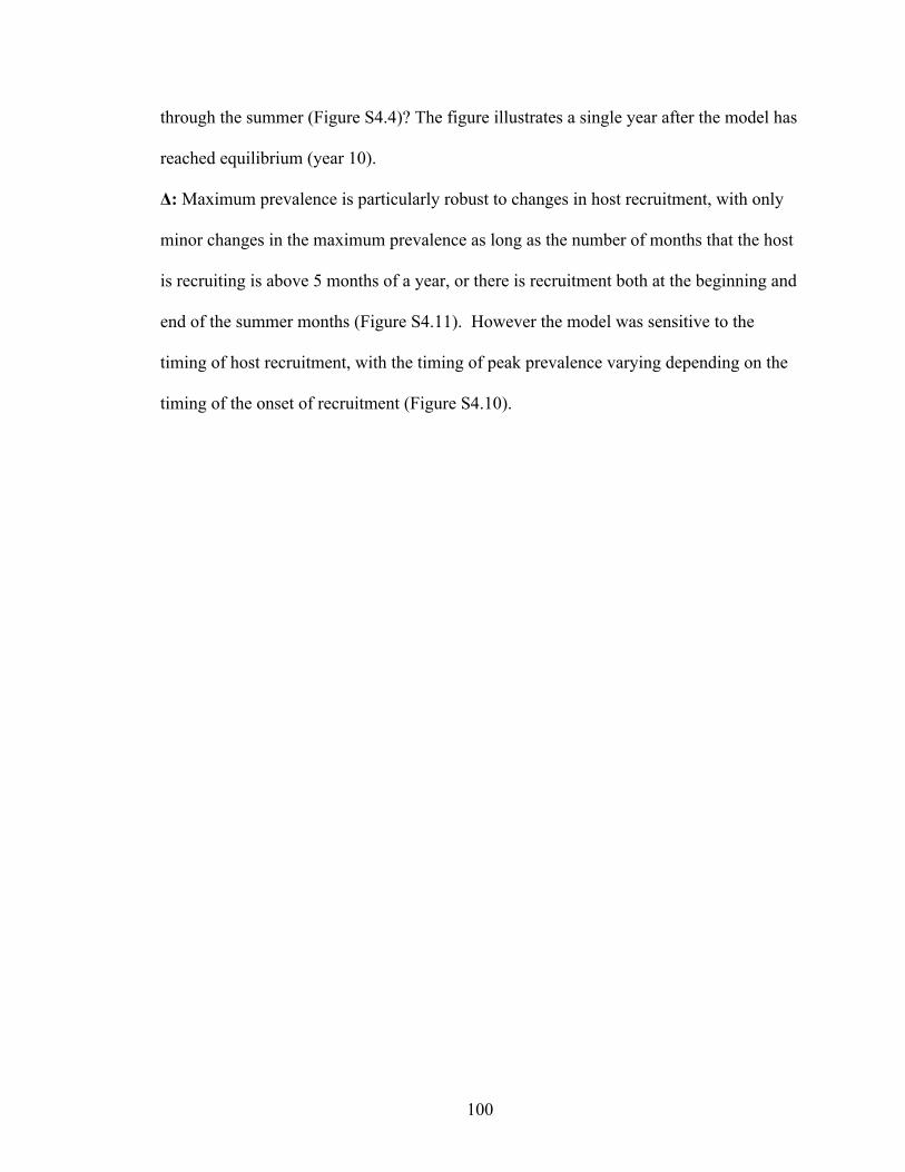
100

through the summer (Figure S4.4)? The figure illustrates a single year after the model has

reached equilibrium (year 10).

Δ: Maximum prevalence is particularly robust to changes in host recruitment, with only

minor changes in the maximum prevalence as long as the number of months that the host

is recruiting is above 5 months of a year, or there is recruitment both at the beginning and

end of the summer months (Figure S4.11). However the model was sensitive to the

timing of host recruitment, with the timing of peak prevalence varying depending on the

timing of the onset of recruitment (Figure S4.10).

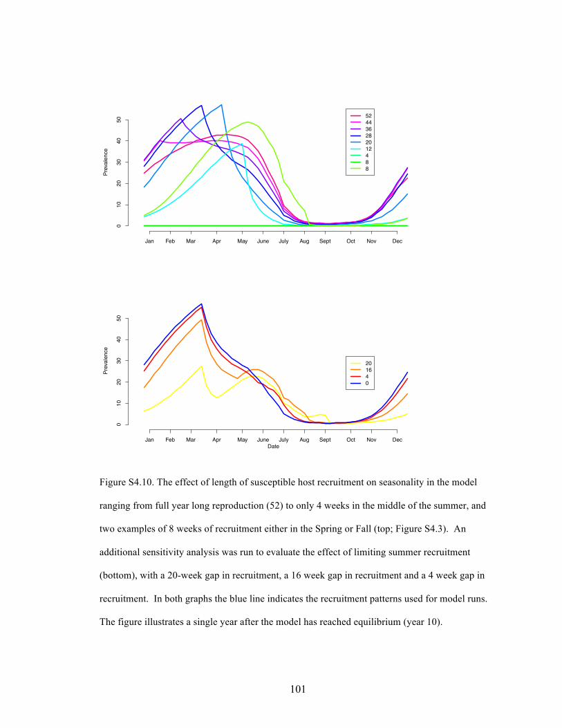
101

Figure S4.10. The effect of length of susceptible host recruitment on seasonality in the model

ranging from full year long reproduction (52) to only 4 weeks in the middle of the summer, and

two examples of 8 weeks of recruitment either in the Spring or Fall (top; Figure S4.3). An

additional sensitivity analysis was run to evaluate the effect of limiting summer recruitment

(bottom), with a 20-week gap in recruitment, a 16 week gap in recruitment and a 4 week gap in

recruitment. In both graphs the blue line indicates the recruitment patterns used for model runs.

The figure illustrates a single year after the model has reached equilibrium (year 10).

Prevalence

010

2030

4050

Jan Feb Mar Apr May June July Aug Sept Oct Nov Dec

524436282012488

Prevalence

010

2030

4050

Jan Feb Mar Apr May June July Aug Sept Oct Nov DecDate

201640

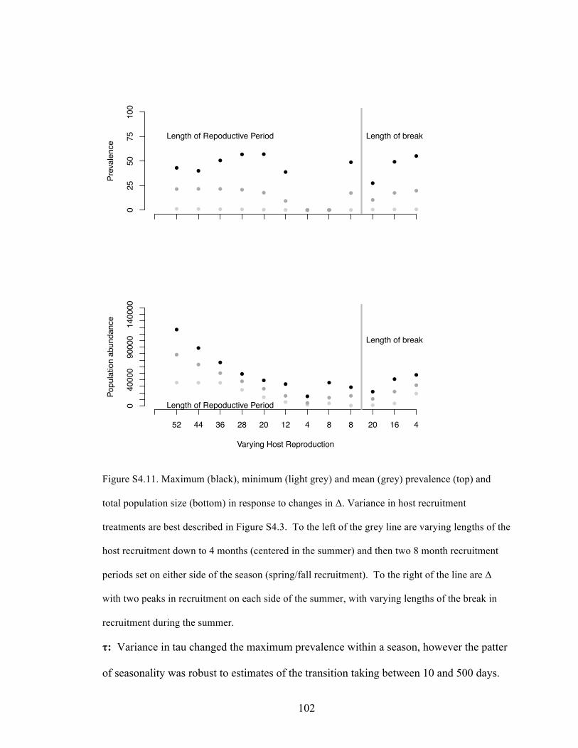
102

Figure S4.11. Maximum (black), minimum (light grey) and mean (grey) prevalence (top) and

total population size (bottom) in response to changes in Δ. Variance in host recruitment

treatments are best described in Figure S4.3. To the left of the grey line are varying lengths of the

host recruitment down to 4 months (centered in the summer) and then two 8 month recruitment

periods set on either side of the season (spring/fall recruitment). To the right of the line are Δ

with two peaks in recruitment on each side of the summer, with varying lengths of the break in

recruitment during the summer.

τ: Variance in tau changed the maximum prevalence within a season, however the patter

of seasonality was robust to estimates of the transition taking between 10 and 500 days.

Prev

alen

ce

●

●

●

●

●

●

●

●

●

●

●

●

●

●

●

●

●

●

●●● ●●●

●

●

●

●

●

●

●

●

●

●

●

●

025

5075

100

Length of Repoductive Period Length of break

Varying Host Reproduction

Popu

latio

n ab

unda

nce

●

●

●

●

●

● ●

●

● ●

●

● ●

●

●●

●

● ●

●●

●

●●

●

●

●●

●

●

●

●

●

●

●

●

040

000

9000

014

0000

52 44 36 28 20 12 4 8 8 20 16 4

Length of Repoductive Period

Length of break

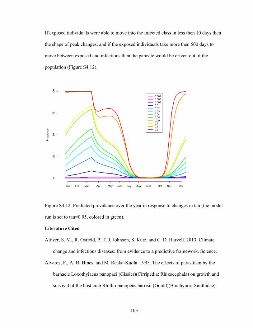
103

If exposed individuals were able to move into the infected class in less then 10 days then

the shape of peak changes, and if the exposed individuals take more then 500 days to

move between exposed and infectious then the parasite would be driven out of the

population (Figure S4.12).

Figure S4.12. Predicted prevalence over the year in response to changes in tau (the model

run is set to tau=0.05, colored in green).

Literature Cited

Altizer, S. M., R. Ostfeld, P. T. J. Johnson, S. Kutz, and C. D. Harvell. 2013. Climate

change and infectious diseases: from evidence to a predictive framework. Science.

Alvarez, F., A. H. Hines, and M. Reaka-Kudla. 1995. The effects of parasitism by the

barnacle Loxothylacus panopaei (Gissler)(Cirripedia: Rhizocephala) on growth and

survival of the host crab Rhithropanopeus harrisii (Gould)(Brachyura: Xanthidae).

Prevalence

025

5075

100

Jan Feb Mar Apr May June July Aug Sept Oct Nov Dec

0.0010.0050.0090.010.020.030.040.050.090.10.50.9

104

Journal of Experimental Marine Biology and Ecology 192:221–232.

Amarasekare, P., and R. Sifuentes. 2012. Elucidating the temperature response of

survivorship in insects. Functional Ecology 26:959–968.

Anderson, R. M., and R. M. May. 1979. Prevalence of schistosome infections within

molluscan populations: observed patterns and theoretical predictions. Parasitology.

Anderson, R. M., and R. M. May. 1982. Coevolution of hosts and parasites. Parasitology

85 (Pt 2):411–426.

Briere, J.-F., P. Pracros, A.-Y. L. Roux, and J.-S. Pierre. 1999. A Novel Rate Model of

Temperature-Dependent Development for Arthropods. Environmental Entomology

28:22–29.

Byers, J. E., J. H. Grabowski, M. F. Piehler, A. R. Hughes, H. W. Weiskel, J. C. Malek,

and D. L. Kimbro. 2015. Geographic variation in intertidal oyster reef properties and

the influence of tidal prism. Limnology and Oceanography:1–19.

Christensen, J. H., B. Hewitson, and A. Busuioc. 2007. Regional climate projections.

Climate Change.

Costlow, J., and C. Bookhout. 1961. The Larval Development of Eurypanopeus

Depressus (Smith) Under Laboratory Conditions 1). Crustaceana 2:6–15.

Dell, A. I., S. Pawar, and V. M. Savage. 2011. Systematic variation in the temperature

dependence of physiological and ecological traits. Proceedings of the National

Academy of Sciences 108:10591–10596.

Di Iorio, D. 2012, January 1. Continuous salinity, temperature and depth measurements

from moored hydrographic data loggers deployed at GCE10_Hydro (Duplin River

west of Sapelo Island, Georgia) from 01-Jan-2011 through 31-Dec-2011. Georgia

105

Coastal Ecosystems LTER Project; University of Georgia; Long Term Ecological

Research Network.

Di Iorio, D. 2013, January 1. Continuous salinity, temperature and depth measurements

from moored hydrographic data loggers deployed at GCE10_Hydro (Duplin River

west of Sapelo Island, Georgia) from 01-Jan-2012 through 31-Dec-2012. Georgia

Coastal Ecosystems LTER Project; University of Georgia; Long Term Ecological

Research Network.

Di Iorio, D. 2014a, January 1. Continuous salinity, temperature and depth measurements

from moored hydrographic data loggers deployed at GCE10_Hydro (Duplin River

west of Sapelo Island, Georgia) from 01-Jan-2013 through 31-Dec-2013. Georgia

Coastal Ecosystems LTER Project; University of Georgia; Long Term Ecological

Research Network.

Di Iorio, D. 2014b, January 1. Continuous salinity, temperature and depth measurements

from moored hydrographic data loggers deployed at GCE10_Hydro (Duplin River

west of Sapelo Island, Georgia) from 01-Jan-2014 through 31-Dec-2014. Georgia

Coastal Ecosystems LTER Project; University of Georgia; Long Term Ecological

Research Network.

Epifanio, C. E., and C. Tilburg. 2008. Transport of blue crab larvae in the Middle

Atlantic Bight: A wet and windy journey. Journal of Marine Research 66:723–749.

Glenner, H. 2001. Cypris metamorphosis, injection and earliest internal development of

the Rhizocephalan Loxothylacus panopaei (Gissler). Crustacea: Cirripedia:

Rhizocephala: Sacculinidae. Journal of Morphology 249:43–75.

Grant, J., and J. McDonald. 1979. Desiccation tolerance ofEurypanopeus depressus

106

(smith)(Decapoda: Xanthidae) and the exploitation of microhabitat. Estuaries and

Coasts 2:172–177.

Harvell, C. D., C. Mitchell, J. R. Ward, S. M. Altizer, A. P. Dobson, R. S. Ostfeld, and

M. D. Samuel. 2002. Climate Warming and Disease Risks for Terrestrial and Marine

Biota. Science 296:2158–2162.

Hoeg, J. T. 1995. The biology and life cycle of the rhizocephala (Cirripedia). Journal of

Marine Biological Association of the UK 75:517–550.

Hudson, P. J., and J. Greenman. 1998. Competition mediated by parasites: biological and

theoretical progress. Trends in Ecology and Evolution 13:387.

Huey, R. B., and J. G. Kingsolver. 1989. Evolution of thermal sensitivity of ectotherm

performance. Trends in Ecology and Evolution 4:131–135.

Huey, R. B., and R. D. Stevenson. 1979. Integrating Thermal Physiology and Ecology of

Ectotherms: A Discussion of Approaches. American Zoologist 19:357–366.

Hulathduwa, Y. D., W. B. Stickle, and K. M. Brown. 2007. The effect of salinity on

survival, bioenergetics and predation risk in the mud crabs Panopeus simpsoni and

Eurypanopeus depressus. Marine Biology 152:363–370.

Johnson, L. R., T. Ben-Horin, K. D. Lafferty, A. Mcnally, E. A. Mordecai, K. P.

Paaijmans, S. Pawar, and S. J. Ryan. 2015. Understanding uncertainty in temperature

effects on vector-borne disease: a Bayesian approach 96:203–213.

Jones, M. B., and C. E. Epifanio. 1995. Settlement of brachyuran megalopae in Delaware

Bay: an analysis of time series data. Estuaries. Marine ecology progress series.

Oldendorf.

Kaplan, A., S. Rebhal, K. D. Lafferty, and A. M. Kuris. 2009. Small estuarine fishes feed

107

on large trematode cercariae: lab and field investigations. Journal Of Parasitology

95:477–480.

Karl, T., J. Melillo, and T. Peterson. 2009. Global climate change impacts in the United

States.

Kruse, H. H., M. Hare, and A. H. Hines. 2011. Genetic relationships of the marine

invasive crab parasite Loxothylacus panopaei: an analysis of DNA sequence

variation, host specificity, and distributional range. Biological Invasions 14:701–715.

LaDeau, S. L., B. F. Allan, P. T. Leisnham, and M. Z. Levy. 2015. The ecological

foundations of transmission potential and vector-borne disease in urban landscapes.

Functional Ecology 29:889–901.

Lafferty, K. D., and A. K. Morris. 1996. Altered behavior of parasitized Killifish

increases susceptibility to predation by bird final hosts. Ecology 77:1390–1397.

McDonald, J. 1982. Divergent Life History Patterns in Co-Occuring Intertidal Crabs

Panopeus herbstii and Eurypanopeus depressus (Crustacea: Brachyura: Xanthidae).

Marine Ecological Progress Series 8:173–180.

Miner, R., S. G. Tolley, and A. Hurley. 2013. Influence of freshwater inflow on

reproductive capacity of the mud crab Eurypanopeus depressus inhabiting oyster

reefs. Journal of Crustacean Biology 33:36–41.

Molnár, P. K., S. J. Kutz, B. M. Hoar, and A. P. Dobson. 2012. Metabolic approaches to

understanding climate change impacts on seasonal host-macroparasite dynamics.

Ecology Letters 16:9–21.

Mordecai, E. A., K. P. Paaijmans, L. R. Johnson, C. Balzer, T. Ben-Horin, E. De Moor,

A. Mcnally, S. Pawar, S. J. Ryan, T. C. Smith, and K. D. Lafferty. 2013. Optimal

108

temperature for malaria transmission is dramatically lower than previously predicted.

Ecology Letters 16:22–30.

Morley, N. J., and J. W. Lewis. 2014. Thermodynamics of trematode infectivity.

Parasitology 142:585–597.

O'Shaughnessy, K. A., D. Freshwater, and E. Burge. 2014a. Prevalence of the Invasive

Rhizocephalan Parasite Loxothylacus panopaei in Eurypanopeus depressus in South

Carolina and Genetic Relationships of the Parasite in North and South Carolina. The

Journal of Parasitology 100:447–454.

O'Shaughnessy, K. A., J. M. Harding, and E. J. Burge. 2014b. Ecological effects of the

invasive parasite Loxothylacus panopaei on the flatback mud crab Eurypanopeus

depressus with implications for estuarine communities. Bulletin of Marine Science

90:611–621.

Paull, S. H., T. R. Raffel, B. E. LaFonte, and P. T. J. Johnson. 2015. How temperature

shifts affect parasite production: testing the roles of thermal stress and acclimation.

Functional Ecology 29:941–950.

Prezant, R., R. Toll, H. Rollins, and E. Chapman. 2002. Marine macroinvertebrate

diversity of St. Catherines Island, Georgia. American Museum Novitates:1–31.

R Development Core Team. 2015, January 1. R: A language and environment for

statistical computing. Vienna, Austria.

Ren, Z., D. Wang, A. Ma, J. Hwang, A. Bennett, H. J. W. Sturrock, J. Fan, W. Zhang, D.

Yang, X. Feng, Z. Xia, X.-N. Zhou, and J. Wang. 2016. Predicting malaria vector

distribution under climate change scenarios in China: Challenges for malaria

elimination. Nature Publishing Group:1–13.

109

Rohr, J. R., A. Dobson, P. T. J. Johnson, A. Kilpatrick, S. H. Paull, T. Raffel, D. Ruiz-

Moreno, and M. Thomas. 2011. Frontiers in climate change-disease research. Trends

in Ecology and Evolution.

Royston, P., and M. K. B. Parmar. 2011. The use of restricted mean survival time to

estimate the treatment effect in randomized clinical trials when the proportional

hazards assumption is in doubt. Statistics in Medicine 30:2409–2421.

Sears, M. W., E. Raskin, and M. J. Angilletta Jr. 2011. The world is not flat: defining

relevant thermal landscapes in the context of climate change. Integrative and

Comparative Biology 51:666–675.

Sulkin, S. 1984. Behavioral basis of depth regulation in hatching and post-larval stages of

the mud crab Eurypanopeus depressus. Marine ecology progress series. Oldendorf

15:181–205.

Tolley, S. G., A. K. Volety, M. Savarese, L. D. Walls, C. Linardich, and E. M. Everham

Iii. 2006. Impacts of salinity and freshwater inflow on oyster-reef communities in

Southwest Florida. Aquatic Living Resources 19:371–387.

Walker, G. 2001. Introduction to the rhizocephala (Crustacea: Cirripedia). Journal of

Morphology 249:1–8.

Walker, G., A. Clare, D. Rittschof, and D. Mensching. 1992. Aspects of the life-cycle of

Loxothylacus panopaei (Gissler), a sacculinid parasite of the mud crab

Rhithropanopeus harrisii (Gould): a laboratory study. Journal of Experimental

Marine Biology and Ecology 157:181–193.

Wood, C. L., and P. T. J. Johnson. 2015. A world without parasites: exploring the hidden

ecology of infection. Frontiers in Ecology and the Environment 13:425–434.

110

CHAPTER 5

CONCLUSION

The outcomes of species interactions are context dependent; whether the predator

captures its prey (Sanford et al. 2014), the effect of a grazers consumption (Ruesink

1998), and whether a parasite infects its host (Blanford et al. 2003). This dissertation

explored the abiotic and biotic drivers that influence the outcomes of host-parasite

interactions, across large-scales (Chapter 1), mechanistically evaluating predator-prey-

parasite interactions within an estuary (Chapter 2) and exploring climate change impacts

on host-parasite dynamics (Chapter 3 and 4).

At a large-scale I demonstrated that a variety of mechanisms influence E.

depressus probability of infection by L. panopaei. The results of this work provide

insight into factors that should be considered when attempting to manage and control

parasite populations. For example, we found that high water movement over a reef was

correlated with higher probability of infection, suggesting that it is important to consider

the rate of ‘recruitment’ of parasite propagules to an area (Chapter 2). I also found

evidence to support density dependence in this system, with infection prevalence

increasing with host density. We explored the relationship between parasite and host

density further, demonstrating that there appears to be an upper limit around 35%

(Chapter 2). A next step will be to explore if this is an emergent property of host-parasite

111

interactions (e.g. do all density dependant systems have limits?) or does finding a limit

indicate something unique about that host-parasite interaction (e.g. that a parasite is

regulating the host population).

Both through large-scale patterns and local mechanistic studies, I expanded the

healthy herd hypothesis into invasion ecology, demonstrating that native predators

preferentially consume an invasive parasite (Chapter 3). The outcome predator-prey-

parasite interactions are far from determined, with field evidence of predators enhancing

(Cáceres et al. 2009, Hawlena et al. 2010), suppressing (Packer et al. 2003, Lafferty

2015) and having no effect on parasites (Duffy 2007, Rohr et al. 2015). This is the first

work to explore the effect of predators on invasive parasites, and it will be important to

see if the range of interactions between invading parasite and predators is as wide as that

seen in native predator-prey-parasite interactions.

Finally, through the combination of lab experiments and epidemiological

modeling I was able to expand ideas of ecophysiology, thermal ecology and disease

ecology to a marine host-parasite interaction, exploring the effects of temperature on

host-parasite dynamics. While thermal ecology has begun to be explored in the debate on

how host-parasite interactions will respond to climate change (Blanford and Thomas

1999, Molnár et al. 2012, Mordecai et al. 2013), empirical evidence lacks far behind

(Altizer et al. 2013). By considering the host and multiple stages of the parasites

performance response across the full range of temperatures experience in the field, it is

possible to both explain why at some points there is a clear, positive relationship between

increased temperature and disease, and yet at the highest temperatures we are also seeing

a loss of disease (Chapter 4).

112

In Chapter 4, I elucidated new patterns of thermal response. External stressors

(either biotic or abiotic) might decrease the thermal breadth, the temperature range over

which an organism has positive performance, or decrease the thermal optima of an

organism. I found that there was a decrease in the thermal breadth of infected host

survival, and I also saw a shift in the thermal survival optima to substantially below that

of the uninfected host. The consequences of this offset in performance are dire for the

parasite, with infected hosts unable to survive simulated climate change scenarios of over

a 3ºC increase in temperature (Chapter 4). It has yet to be seen whether this mismatch in

performance between infected and uninfected hosts is a general trend. The shape and

response of ectothermic hosts to temperature has been long evaluated and shows large-

scale generalities (Huey and Kingsolver 1989, Angilletta et al. 2002), and it will be

exciting to see if and how generalities can be applied across interacting species.

Through this dissertation I have demonstrated that both abiotic and biotic drivers

affect host-parasite interactions. I have used a single host-parasite system to explore and

expand on ideas from across the field of ecology, from invasion, to disease, to thermal

and physiological ecology. Through combining fields I have found new host-parasite

patterns, from a potential upper limit to infection prevalence based on host density, to an

offset in thermal performance between infected and healthy hosts. Future work exploring

the generalities of these patterns will elucidate whether these are unique to this host-

parasite pairing, or whether they represent new emergent patterns of host-parasite

ecology.

Literature Cited

Altizer, S. M., R. Ostfeld, P. T. J. Johnson, S. Kutz, and C. Harvell. 2013. Climate

113

change and infectious diseases: from evidence to a predictive framework. Science.

Angilletta, M. J., Jr, P. H. Niewiarowski, and C. A. Navas. 2002. The evolution of

thermal physiology in ectotherms. Journal of Thermal Biology 27:249–268.

Blanford, S., and M. B. Thomas. 1999. Host thermal biology: the key to understanding

host–pathogen interactions and microbial pest control? Agricultural and Forest

Entomology 1:195–202.

Blanford, S., M. B. Thomas, C. Pugh, and J. K. Pell. 2003. Temperature checks the Red

Queen? Resistance and virulence in a fluctuating environment. Ecology Letters 6:2–

5.

Cáceres, C. E., C. J. Knight, and S. R. Hall. 2009. Predator-spreaders: predation can

enhance parasite success in a planktonic host-parasite system. Ecology 90:2850–

2858.

Duffy, M. A. 2007. Selective predation, parasitism, and trophic cascades in a bluegill-

Daphnia-parasite system. Oecologia 153:453–460.

Hawlena, D., Z. Abramsky, and A. Bouskila. 2010. Bird predation alters infestation of

desert lizards by parasitic mites. Oikos 119:730–736.

Huey, R. B., and J. G. Kingsolver. 1989. Evolution of thermal sensitivity of ectotherm

performance. Trends in Ecology and Evolution 4:131–135.

Lafferty, K. D. 2015. Fishing for Lobsters Indirectly Increases Epidemics in Sea Urchins

. Ecological Applications 14:1566–1573.

Molnár, P. K., S. J. Kutz, B. M. Hoar, and A. P. Dobson. 2012. Metabolic approaches to

understanding climate change impacts on seasonal host-macroparasite dynamics.

Ecology Letters 16:9–21.

114

Mordecai, E. A., K. P. Paaijmans, L. R. Johnson, C. Balzer, T. Ben-Horin, E. De Moor,

A. Mcnally, S. Pawar, S. J. Ryan, T. C. Smith, and K. D. Lafferty. 2013. Optimal

temperature for malaria transmission is dramatically lower than previously predicted.

Ecology Letters 16:22–30.

Packer, C., R. D. Holt, P. J. Hudson, K. D. Lafferty, and A. P. Dobson. 2003. Keeping

the herds healthy and alert: implications of predator control for infectious disease.

Ecology Letters 6:797–802.

Rohr, J. R., D. J. Civitello, P. W. Crumrine, N. T. Halstead, A. D. Miller, A. M.

Schotthoefer, C. Stenoien, L. B. Johnson, and V. R. Beasley. 2015. Predator

diversity, intraguild predation, and indirect effects drive parasite transmission

112:3008–3013.

Ruesink, J. L. 1998. Variation in per capita interaction strength: thresholds due to

nonlinear dynamics and nonequilibrium conditions. Proceedings of the National

Academy of Sciences of the United States of America 95:6843–6847.

Sanford, E., B. Gaylord, A. Hettinger, E. A. Lenz, K. Meyer, and T. M. Hill. 2014. Ocean

acidification increases the vulnerability of native oysters to predation by invasive

snails. Proceedings of the Royal Society B: Biological Sciences 281:20132681–

20132681.