Communications in Statistics - Theory and Methods …cucala/agregats3D.pdfMultiple Spatio-Temporal Cluster Detection for Case ... Theory and Methods, 40: 2, 358 — 372 To link

PLEASE SCROLL DOWN FOR ARTICLE

This article was downloaded by: [Cucala, Lionel]On: 22 October 2010Access details: Access Details: [subscription number 928470289]Publisher Taylor & FrancisInforma Ltd Registered in England and Wales Registered Number: 1072954 Registered office: Mortimer House, 37-41 Mortimer Street, London W1T 3JH, UK

Communications in Statistics - Theory and MethodsPublication details, including instructions for authors and subscription information:http://www.informaworld.com/smpp/title~content=t713597238

Multiple Spatio-Temporal Cluster Detection for Case Event Data: AnOrdering-Based ApproachC. Dematteia; L. Cucalab

a Medical Information Department, Nimes University Hospital Center, Nimes, France b Institute ofMathematics and Modelling of Montpellier, Montpellier, France

Online publication date: 21 October 2010

To cite this Article Demattei, C. and Cucala, L.(2011) 'Multiple Spatio-Temporal Cluster Detection for Case Event Data:An Ordering-Based Approach', Communications in Statistics - Theory and Methods, 40: 2, 358 — 372To link to this Article: DOI: 10.1080/03610920903411200URL: http://dx.doi.org/10.1080/03610920903411200

Full terms and conditions of use: http://www.informaworld.com/terms-and-conditions-of-access.pdf

This article may be used for research, teaching and private study purposes. Any substantial orsystematic reproduction, re-distribution, re-selling, loan or sub-licensing, systematic supply ordistribution in any form to anyone is expressly forbidden.

The publisher does not give any warranty express or implied or make any representation that the contentswill be complete or accurate or up to date. The accuracy of any instructions, formulae and drug dosesshould be independently verified with primary sources. The publisher shall not be liable for any loss,actions, claims, proceedings, demand or costs or damages whatsoever or howsoever caused arising directlyor indirectly in connection with or arising out of the use of this material.

http://www.informaworld.com/smpp/title~content=t713597238

http://dx.doi.org/10.1080/03610920903411200

http://www.informaworld.com/terms-and-conditions-of-access.pdf

Communications in Statistics—Theory and Methods, 40: 358–372, 2011Copyright © Taylor & Francis Group, LLCISSN: 0361-0926 print/1532-415X onlineDOI: 10.1080/03610920903411200

Multiple Spatio-Temporal Cluster Detectionfor Case Event Data: An Ordering-Based Approach

C. DEMATTEI1 AND L. CUCALA2

1Medical Information Department, Nimes University Hospital Center,Nimes, France2Institute of Mathematics and Modelling of Montpellier,Montpellier, France

This article introduces a spatio-temporal distance which allows the extension ofthe spatial cluster detection methods of Demattei et al. (2007) and Cucala (2009).A review of these methods is given before we define a spatio-temporal distance.Then this distance is used for detecting spatio-temporal clusters. These ordering-based methods are compared to the scan statistic by a simulation study. Thescan procedure is more powerful but it detects fewer true positives due to itslack of flexibility. Those techniques are applied to a seismic data set. This articlehighlights two advantages of the ordering-based methods: their flexibility and theirlow computational demand.

Keywords Case event data; Cluster detection; Ordering-based methods; Spatio-temporal distance.

Mathematics Subject Classification 62P99.

1. Introduction

The spatio-temporal cluster detection is a recent development which deserves allthe interest successively given to the detection of clusters in time, then in space. Asin the spatial setting, several methods, notably derived from the scan statistic, areproposed.

Several procedures have been developed in order to study the spatio-temporalaggregation of geographical health data. The interaction test proposed by Knox(1964) is a precocious approach of this type of test. This test is a global methodsince potential clusters cannot be located.

The first real approach that allows researchers to locate and detect a spatio-temporal cluster is certainly the spatio-temporal scan statistic introduced byKulldorff (1998) which is a direct adaptation of the spatial scan statistic. Instead of

Received October 1, 2008; Accepted October 13, 2009Address correspondence to C. Demattei, Departement de I’Information Medicale,

Batiment Polyvalent, CHU Caremeau, 30029 Nimes, France; E-mail: [email protected]

358

Downloaded By: [Cucala, Lionel] At: 08:45 22 October 2010

Spatio-Temporal Cluster Detection 359

using circular windows, cylinders are chosen for potential cluster shape. The circularbasis represents the spatial area and the height of the cylinder represents the timeperiod.

Other approaches have also been proposed such as the method of Iyengar(2004) that uses the scan statistic to search for pyramidal-shaped clusters. All thosemethods have advantages and drawbacks. We may blame the scan statistic fornot being flexible. Other methods are more flexible but need more computationalresources. Let us recall that the spatio-temporal cluster detection domain is quitenew and lots of improvement are to be done, as it was the case in the spatial setting.

The core of this article is the definition of a spatio-temporal distance whichmakes it possible to generalize the spatial cluster detection methods for case eventdata of Demattei et al. (2007) and Cucala (2009).

We first define a general framework for those two methods denoted by“ordering-based methods”. Indeed, those approaches have in common to be thespatial adaptation of a temporal cluster detection technique, and this generalizationis achieved by a common data transformation (Demattei et al., 2007) that makes itpossible to order spatial events.

Once this framework is defined, we extend both spatial ordering-based methodsto the spatio-temporal setting by introducing a spatio-temporal distance that allowsus to order events both in space and time.

A simulation power study is then proposed to compare the ordering-basedmethods to the spatio-temporal scan statistic, which is the reference method. Thescan statistic is widely used to locate and detect spatio-temporal clusters of medicalevents as for example in McNally and Colver (2008) and Demattei et al. (2006a).The scan statistic is a very powerful method, but the parametric shape of thepotential clusters (usually cylinders) reduces its flexibility and increases considerablythe computational time compared to non-parametric methods such as ordering-based procedures. The flexibility of ordering-based methods is illustrated on a“L”-shaped example.

Those three techniques are also applied to a seismic data set. This data set is anItaly Catalogue of Earthquake Events included in the Statistical Seismology Library(SSLib) provided in R format by David Harte and Ray Brownrigg.

Finally, a computing time comparison is proposed between ordering-based andscan methods. A discussion concludes this article.

2. 2D and 3D Spatial Cluster Detection

2.1. The Spatial Scan Statistic

The most popular of the spatial cluster detection methods is the spatial scanstatistic (Kulldorff, 1997). It relies on restricting the set of possible clusters to afinite family of subsets of the observation area. Then, the concentration in eachof these subsets is assessed through the likelihood ratio test of H0, the hypothesisthat cases are distributed as the underlying population, against a specific piecewise-constant density alternative. Originally, the possible clusters family was set to allthe circles whose centers were points of a predefined grid. Recently, Kulldorff et al.(2006) extended the method by investigating a wide family of elliptic windows withpredetermined shape, angle and center.

A multiple procedure has also been introduced (Zhang et al., 2010) and allowsusers for testing the significativity of secondary clusters. Even if no theoretical


360 Demattei and Cucala

justification exists, a simulation study shows that the Type I error of this procedureremains close to the nominal level.

Even if these methods were first defined to study aggregated data, they alsoadapt to case event data. However, when the number of events becomes large, theset of possible clusters increases dramatically, and so does the computation time.

2.2. Introduction to Ordering-Based Spatial Methods

Spatial methods are often adapted from existing temporal cluster detectiontechniques, as for regression (Demattei et al., 2007) and spacings (Cucala, 2009)methods. In the temporal setting, the time of occurrence of events can be consideredas a natural way to order events between them. In the spatial case, such a naturalorder does not exist. A data transformation is then needed to order spatial eventsand be able to adapt temporal techniques to spatial data. Those approaches arecalled ordering-based spatial methods. The regression and spacings methods belongto this class of spatial cluster detection methods.

The same data transformation is used for both approaches. Let �X1� � � � � Xn� berandom variables which denote the spatial coordinates of the occurrence of n eventsin A, a bounded set of �2 or �3. The first ordered event X�1� is arbitrarily chosento be the nearest point from the boundary of A, denoted by �A, using the euclidiandistance, denoted by d�� . Thus,

D0 = d�X�1�� A� = min1≤i≤n

d�Xi� �A��

Then the second event, whose location is called X�2�, is the closest to X�1� among allthe events that have not yet been ordered, such that

D1 = d�X�2�� X�1�� = min1≤i≤nXi �=X�1�

d�Xi� X�1��

All the events are iteratively ordered in the same way and

Dj = d�X�j+1�� X�j�� = min1≤i≤n

Xi �=X�k�� ∀k=1��j−1

d�Xi� X�j−1�� ∀j = 2� � � � � n− 1�

The �D1� � � � � Dn−1� series is then used by both approaches to detect portionswith small successive distances. This is described in the following sections.

2.3. The Regression Method

The spatial regression method (Demattei et al., 2007) is an adaptation of a multipletemporal cluster detection procedure (Molinari et al., 2001).

Let dk = d�x�k+1�� x�k�� be a realization of Dk. This distance has to be weightedboth to correct the presence of high distances due to the elimination process ofpre-selected points and to adjust for a potential inhomogeneity in the underlyingpopulation density. The weighted distance dw

k is defined as the ratio between the



distance dk and its expectation under H0. Demattei et al. (2007) showed that theexpected distance can be written

EH0

[Dk/X�1� = x�1�� X�k� = x�k�

] = ∫ a

0

[1−

∫Ak−1∩S�x�k��r� f�x�dx∫

Ak−1f�x�dx

]n−k

dr� (1)

where f�x� stands for the underlying population density from which the n points areindependently sampled, S�x� r� is the sphere with center x and radius r, and Ak =A\ {⋃k

i=1 S�x�i�� di�}with the convention A0 = A.

The numerical integration of∫ a

0 in Eq. (1) is achieved by using the trapezoidalrule. Moreover, the underlying population Z, constituted by N individuals �zi � i =1� � � � � N�, makes it possible to estimate the density integrals

∫Ak−1

and∫Ak−1∩S�x�k��r�.

Indeed, for any set B ⊂ A,∫Bf�x�dx can be approximated by #�i/zi ∈ B�/N . This

integral approximation makes it possible to adjust the computation of dwk for

inhomogeneous population. This adjustment is important since, when dealing withrare diseases, a large study area is necessary to examine data for evidence of spatialclustering. Hence, due to a natural inhomogeneity, the density of the population atrisk is not constant over the study area.

Cluster bounds can now be determined from transformed data �k� dwk �k=1��n−1.

For this purpose, we consider the weighted distance regression on the selection orderk. To determine the presence of m breaks (denoted by b1� � � � � bm), the regressionfunction taken into consideration is

f�t� =m+1∑j=1

dbj−1+1bj �× Ibj−1+1bj �

�t� (2)

with the convention b0 = 0 and bm+1 = n− 1. The notation dbj−1+1bj �stands for the

mean of dwt for t in bj−1 + 1 bj�.

The minimum percentage of points between two breaks is a parameter whichhas to be taken into account. Let � ∈ 0 1� denote this parameter. Then, the setof possible partitions is � = ��b1� � � � � bm�; ∀i = 1� � � � � m+ 1, card �bi−1 + 1 bi�� ≥�n− 1��.

Breaks (cluster bounds) are estimated by

�b1� � � � � bm� = argmin�b1��bm�∈ �

n−1∑t=1

�dwt − f�t��2 (3)

and are computed efficiently using a dynamic algorithm programming (Dematteiet al., 2006b).

The double maximum test proposed by Bai and Perron (1998) is used to selectthe best model. This test makes it possible to test the null hypothesis of no breakagainst an unknown number of breaks given a certain upper bound M . Once thebest model is selected, a p-value is computed for each portion between two breaksby a Monte Carlo procedure. The best model selection and the p-value computationare fully described in Secs. 2.5 and 2.6 of the article of Demattei et al. (2007).



2.4. The Spacings Method

This procedure, introduced by Cucala (2009), is also based on the same ordering ofthe spatial events. However, it does not rely on the distances between events, but onthe areas Si explored between events. The first area is defined by

S1 = �x ∈ A � d�x� �A� < D0��

The successive areas are then given by

Si ={x ∈ ⋃

j=1�··· �i−1

Sj � d�x� X�i−1�� < Di−1

}� 2 ≤ i ≤ n�

where B = �x ∈ A � x B�.The area spacings are defined by

S′i =

∫Si

f�s��ds�� 1 ≤ i ≤ n+ 1

and can be estimated using the underlying population Z, as in the regressionmethod. These area spacings follow under H0 the same distribution as uniformspacings (i.e., spacings issued from a 0� 1�-uniform n-sample). Thus, the spatialcluster detection can rely on a temporal cluster detection technique applied to thepoint process �T1� � � � � Tn�, where Ti =

∑ij=1 S

′j . The objective of temporal cluster

detection is to test whether there exists a time interval in which events areabnormally concentrated. The concentration indicator we apply here is the oneintroduced by Cucala (2008). The p-value of the most concentrated interval isestimated by a Monte-Carlo procedure and a multiple procedure makes it possibleto detect secondary clusters. Let Ii = Tai

� Tbi�, 1 ≤ i ≤ k denote the k significative

temporal clusters identified. The corresponding spatial clusters are then the zones

Ci =bi⋃

j=ai+1

Si

and the total clustering zone is

C =k⋃

i=1

Ci�

3. Spatio-Temporal Cluster Detection

3.1. The Spatio-Temporal Scan Statistic

The spatial scan statistic naturally extends to the spatio-temporal setting. Thepossible clusters family is now a collection of cylindrical windows with a circular(or elliptic) geographic base and with height corresponding to time. Then, theconcentration in each of these windows is assessed similarly than in the spatialsetting.

A multiple procedure identical to the spatial one can also be used. Of course,the number of windows to compare is even larger than in the spatial setting



and analysing large case event data sets with this method is computationally veryexpensive.

3.2. Spatio-Temporal Distance Definition

We propose to extend the regression and spacings spatial methods to space-timecluster detection. In this issue, the main difficulty results from the different rolesplayed by the temporal and spatial dimensions.

To overcome this difficulty, we propose introducing a so-called spatio-temporaldistance which is a weighted combination of the spatial and temporal euclidiandistances. A parameter is needed to establish a correspondence between space andtime.

We propose the following choice for the value of this parameter. Let �A� denotethe observation domain area and �T � the time observational interval length. Let D =2√

�A��

the diameter of a disc whose area is �A�. This is nothing but the maximalspatial distance between two points in the disc. Our objective is to consider that atemporal distance equal to �T � between two events is equivalent to a spatial distanceequal to D. Hence, we set the spatio-temporal distance, denoted by dST , to be thefollowing function of the euclidian spatial and temporal distances dS and dT :

dST �x� y� t�� x0� y0� t0��2 = dS�x� y�� x0� y0��

2 + D2

�T �2 dT t� t0�

2�

Intuitively, this distance can be seen as a spatial euclidian distance in�3 after rescaling the temporal axis. More rigorously, dST �x� y� t�� x0� y0� t0�� =dS�x� y� D

Tt�� x0� y0�

DTt0�� which ensures that dST is a distance.

3.3. Ordering-Based Spatio-Temporal Methods

For k = 1� � � � � n, Zk = �Xk� Tk� denotes the spatial and temporal coordinates of aspatio-temporal event in a bounded set of A× T ∈ �s ×�, with s = 2 or 3. Theregression and spacings method previously described are applied to these data,replacing the spatial euclidian distance by the spatio-temporal distance we justintroduced.

4. Simulations

In this section, all samples were simulated with A = 0 1�× 0 1� (space) and T =�1� 2� � � � � 31� (time = one month in days).

The Type I error rate was obtained on 500 samples simulated under theno-clustering hypothesis (H0).

A power study was performed using several aggregation alternatives. For eachalternative, 100 samples of 200 points were simulated . The time of occurrence of theevents follows a discrete uniform distribution on T . In the clustering alternatives,the spatial locations follow a mixture of two uniform point processes, depending onthe time interval, as described in Table 1.

The cluster simulation zones for each cluster alternative are illustrated in Fig. 1.



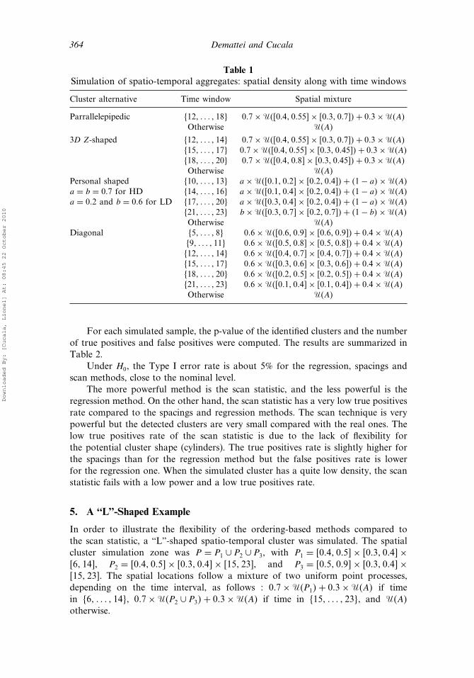
Table 1Simulation of spatio-temporal aggregates: spatial density along with time windows

Cluster alternative Time window Spatial mixture

Parrallelepipedic �12� � � � � 18� 0�7×��0�4� 0�55�× 0�3� 0�7��+ 0�3×��A�Otherwise ��A�

3D Z-shaped �12� � � � � 14� 0�7×��0�4� 0�55�× 0�3� 0�7��+ 0�3×��A��15� � � � � 17� 0�7×��0�4� 0�55�× 0�3� 0�45��+ 0�3×��A��18� � � � � 20� 0�7×��0�4� 0�8�× 0�3� 0�45��+ 0�3×��A�Otherwise ��A�

Personal shaped �10� � � � � 13� a×��0�1� 0�2�× 0�2� 0�4��+ �1− a�×��A�a = b = 0�7 for HD �14� � � � � 16� a×��0�1� 0�4�× 0�2� 0�4��+ �1− a�×��A�a = 0�2 and b = 0�6 for LD �17� � � � � 20� a×��0�3� 0�4�× 0�2� 0�4��+ �1− a�×��A�

�21� � � � � 23� b ×��0�3� 0�7�× 0�2� 0�7��+ �1− b�×��A�Otherwise ��A�

Diagonal �5� � � � � 8� 0�6×��0�6� 0�9�× 0�6� 0�9��+ 0�4×��A��9� � � � � 11� 0�6×��0�5� 0�8�× 0�5� 0�8��+ 0�4×��A��12� � � � � 14� 0�6×��0�4� 0�7�× 0�4� 0�7��+ 0�4×��A��15� � � � � 17� 0�6×��0�3� 0�6�× 0�3� 0�6��+ 0�4×��A��18� � � � � 20� 0�6×��0�2� 0�5�× 0�2� 0�5��+ 0�4×��A��21� � � � � 23� 0�6×��0�1� 0�4�× 0�1� 0�4��+ 0�4×��A�Otherwise ��A�

For each simulated sample, the p-value of the identified clusters and the numberof true positives and false positives were computed. The results are summarized inTable 2.

Under H0, the Type I error rate is about 5% for the regression, spacings andscan methods, close to the nominal level.

The more powerful method is the scan statistic, and the less powerful is theregression method. On the other hand, the scan statistic has a very low true positivesrate compared to the spacings and regression methods. The scan technique is verypowerful but the detected clusters are very small compared with the real ones. Thelow true positives rate of the scan statistic is due to the lack of flexibility forthe potential cluster shape (cylinders). The true positives rate is slightly higher forthe spacings than for the regression method but the false positives rate is lowerfor the regression one. When the simulated cluster has a quite low density, the scanstatistic fails with a low power and a low true positives rate.

5. A “L”-Shaped Example

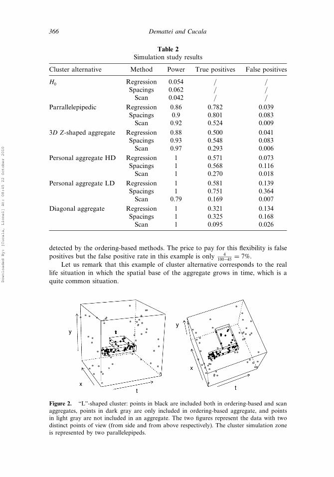
In order to illustrate the flexibility of the ordering-based methods compared tothe scan statistic, a “L”-shaped spatio-temporal cluster was simulated. The spatialcluster simulation zone was P = P1 ∪ P2 ∪ P3, with P1 = 0�4� 0�5�× 0�3� 0�4�×6� 14�, P2 = 0�4� 0�5�× 0�3� 0�4�× 15� 23�, and P3 = 0�5� 0�9�× 0�3� 0�4�×15� 23�. The spatial locations follow a mixture of two uniform point processes,depending on the time interval, as follows : 0�7×��P1�+ 0�3×��A� if timein �6� � � � � 14�, 0�7×��P2 ∪ P3�+ 0�3×��A� if time in �15� � � � � 23�, and ��A�

otherwise.



Figure 1. Simulation cluster alternatives: from top to bottom, parallelepipedic, 3D Zshaped, personalized and diagonal cluster simulation zones.

The ordering-based and scan methods were applied to this simulated data set.The obtained results are illustrated in Fig. 2. The ordering-based methods detect asignificant aggregate made up of 49 events. Fourty-five events (92%) are includedin P. 100% of the cluster events are detected by the ordering-based methods. Thescan statistic detects a significant aggregate of 34 events, all included in P. The scandetects only 76% of points included in P. Indeed, it detects 100% of the events inP1 ∪ P2 but 0% of the events in P3.

This example illustrates the lack of flexibility of the scan statistic compared tothe ordering-based methods. This is due to the parametric shape of the scanningwindow which, here, only detects the lengthened zone P1 ∪ P2 (close to a cylindricshape), and does not detect the P3 zone. In the same time, this “L”-shape is entirely



Table 2Simulation study results

Cluster alternative Method Power True positives False positives

H0 Regression 0.054 / /Spacings 0.062 / /Scan 0.042 / /

Parrallelepipedic Regression 0.86 0.782 0.039Spacings 0.9 0.801 0.083Scan 0.92 0.524 0.009

3D Z-shaped aggregate Regression 0.88 0.500 0.041Spacings 0.93 0.548 0.083Scan 0.97 0.293 0.006

Personal aggregate HD Regression 1 0.571 0.073Spacings 1 0.568 0.116Scan 1 0.270 0.018

Personal aggregate LD Regression 1 0.581 0.139Spacings 1 0.751 0.364Scan 0.79 0.169 0.007

Diagonal aggregate Regression 1 0.321 0.134Spacings 1 0.325 0.168Scan 1 0.095 0.026

detected by the ordering-based methods. The price to pay for this flexibility is falsepositives but the false positive rate in this example is only 4

100−45 = 7%.Let us remark that this example of cluster alternative corresponds to the real

life situation in which the spatial base of the aggregate grows in time, which is aquite common situation.

Figure 2. “L”-shaped cluster: points in black are included both in ordering-based and scanaggregates, points in dark gray are only included in ordering-based aggregate, and pointsin light gray are not included in an aggregate. The two figures represent the data with twodistinct points of view (from side and from above respectively). The cluster simulation zoneis represented by two parallelepipeds.



6. Spatio-Temporal Analysis of Colfiorito Earthquake Sequence

To illustrate those approaches on real data, we used a seismic data set includedin the Statistical Seismology Library (SSlib: a collection of earthquake hypocentralcatalogues and R functions to analyse the catalogues). This data set is made upof 43,000 earthquake events that appeared in Italy from 1983–2006. The datasource is the Istituto Nazionale di Geofisica e Vulcanologia. For each event,latitude, longitude, date, time, and magnitude are given. The earthquake events arerepresented in Fig. 3 along with the two fault lines.

Due to the very high number of events, we selected the earthquake events witha magnitude higher than 4.5 (on the Richter scale). To avoid a selection bias dueto non exhaustivity at the beginning of the study, we also selected the events thatappeared after 1993. Finally, 66 events were selected and analysed with spatial andspatio-temporal cluster detection methods.

The spatial and spatio-temporal regression, spacings and scan methods wereapplied to this data set. All the clusters reported in what follows are significant atthe nominal level of 0�05. Depending on the choice for the underlying population Z,we may take into account the spatial and temporal distribution of the earthquakesor not.

Figures presented in this section use the same legend. Events are representedby a black point. Events located in the regression aggregates are surrounded bya grey disc. Events located in the spacings aggregates are surrounded by a blackcircle. The most likely cluster detected by the scan statistic is represented by anellipse (circle deformed by planar projection). Underlying population individualsare represented by little black points. For spatio-temporal figures, a full line reliestemporally successive events of the north fault aggregate and a triangle denotes thedirection of the temporal evolution.

Figure 3. Colfiorito earthquake sequence: earthquake events are represented by little blackpoints. Full lines materialize south and north fault lines.



6.1. Testing Against Uniformity

Firstly, we chose a uniform 10,000 points random process as the underlyingpopulation Z.

All the spatial cluster detection methods exhibit the same compact clusterlocated along the south fault including nine earthquake events which are spatiallyvery close. The spacings method also detects a second cluster, less compact, alongthe north fault and including 11 events. Those clusters are shown in Fig. 4.

The spatio-temporal regression and spacings methods exhibit two identicalspatio-temporal clusters. The spacings method reveals a third one. The spatio-temporal scan statistic only detects the first cluster located by the ordering-basedmethods. The spatial representation of those clusters is shown in Fig. 5.

The two ordering-based methods and the scan statistic highlight the samecompact cluster (in the south) including nine earthquake events that occurred in1997. This spatio-temporal aggregate is identical to the spatial cluster detected.This result gives more reliability to this spatio-temporal cluster, since spatialaggregated events are also temporally very close. Watching more carefully thosenine aggregated events, we remark that seven out of nine occurred betweenSeptember 26, 1997 and November 9, 1997. September 26, 1997 is exactly the dayof the beginning of the Colfiorito earthquake sequence (magnitude of 6.1). Thissequence presented the peculiarity to be made up of several major earthquakes close(in time and space) from a first earthquake, which is the case for our detectedcluster.

The two ordering-based methods also detect a second cluster along the northfault line. Those nine events are more spread in space (as we can see in Fig. 5) andtime since they occurred between September 12, 2005 and November 7, 2006.

The spacings method detects a third cluster including seven events locatedbetween the two faults. Those events occurred between October 31, 2002 andNovember 25, 2004.

Figure 4. Colfiorito earthquake sequence: spatial clusters detected with regression, spacingsand scan method with uniform underlying population.



Figure 5. Colfiorito earthquake sequence: spatio-temporal clusters detected with regression,spacings and scan methods with uniform underlying population.

6.2. Taking the Spatial and Temporal Distributions Into Account

Secondly, we chose the 43,000 earthquake events that occurred between 1993and 2006 as the underlying population. For the scan statistic, which is computerintensive, we have selected the sub population of events with a magnitude higherthan 2.5, which contains 14,591 events. Making this choice, we may identify theclusters of high-magnitude events among all the events. The underlying population,high magnitude events and aggregated events are represented in Fig. 6.

Figure 6. Colfiorito earthquake sequence: spatio-temporal clusters detected with regression,spacings and scan methods with true underlying population.



The southern cluster has disappeared, but the spread northern one is included inthe exhibited cluster. Those aggregated events correspond to events which occurredalong the north fault line, where the probability for an event to occur is lowcompared to the south fault line. Those results illustrate the importance of thechoice for the underlying population. We also remark that aggregated eventsare temporally ordered from east to west along the north fault line. This resulthighlights the spatio-temporal evolution of an initial earthquake event. The mostlikely spatio-temporal cluster of the scan statistic is not reported here since its spatialradius is 715kms. This cluster is huge compared to the maximal distance betweentwo events, that is 1,750kms.

7. Computing Time

In the previous section, we have asserted that the scan statistic is computer intensive.Even if the SaTScan (Kulldorff and Information Management Services, 2006) userguide specifies that “The spatial and space-time scan statistics are computer intensiveto calculate”, this fact has to be substantiated. For this purpose, we have evaluatedthe computing time for each method on 100 samples of 100 points. The underlyingpopulation size was fixed at 10,000.

The regression method runs very fast since it takes only 11.7 s in average andranges between 11 and 13 s. The spacings method is a little more time-consumingsince it runs in 30.8 s and ranges between 25 and 39 s. Finally, the scan method isvery consuming in computing time. The average is 18.2min, and it ranges between16.7 and 36min. On those data sets, the scan takes about 100 times more time thanthe regression method and 35 times more time than the spacings method.

All the programs run on the same PC. Moreover, while the scan statistic iscomputed by the SaTScan software, which is optimized for reducing computingtime, the ordering-based methods are written in R language, which is quite time-comsuming.

To complete the illustration of the quickness of the ordering-based methods incomparison with the scan statistic, let us remark that the regression method runs in8 s for analysing the “L”-shaped data set studied in Section 5. On the same data set,the scan statistic runs in 38min and 20 s, that is to say 280 times slower.

Even if our demonstration holds true only in the particular case of our data setson our personal computer, let us try to explain such differences on the computingtime. The computational problem of the classical scan statistic is a consequenceof the generation of the possible clusters. Indeed, the SaTScan software takesinto account all the events in order to build the possible clusters, whether theseare case events or control events. Then, the program counts how many case andcontrol events are located in each possible cluster. So, increasing the number ofcontrol events increases both the number of possible clusters and the length of thecounting process in each one. On the other hand, when one applies an ordering-based method, the computation of the areas Ai only depends on the case events.The control events are then counted in each of these areas to compute the weighteddistances dw

k or the area spacings A′i. Thus, increasing the number of control events

increases only the length of the counting process in the ordering-based methods:they become less time-consuming when the control data increases.



8. Discussion

The ordering-based spatio-temporal methods that we have developed and presentedin this article are very flexible. Indeed, the shape of the estimated cluster is notprespecified. This is a great advantage since usually people do not know the kindof cluster they are looking for. The lack of power compared to the scan statistic,illustrated by the simulation study, is balanced by the flexibility and the ability tolocate and detect several arbitrarily-shaped clusters, as shown with the “L”-shapedexample. This flexibility is also illustrated by the application to the seismic dataset: we manage to highlight the evolution of a earthquake event sequence along thenorth fault while the scan statistic fails.

Even if the flexibility of our method is an advantage, some people may preferusing the scan statistic which is a better alarm as it detects more easily the presenceof a cluster. In fact, any user should answer the question: do I prefer detectingthe presence of a cluster without estimating its precise location, or getting a moreprecise location of the cluster without being sure of detecting it? An example ofsituation in which the researcher or user will prefer the second approach is thestudy of the spatio-temporal repartition of paludism cases along a river. Indeed, thevector of the parasite responsible of the human paludism are anopheles which livemainly near water and in damp surroundings. In this case, the use of ordering-basedspatio-temporal methods is clearly indicated to put into evidence the increased riskof contamination along the river. In other situations, the circular or cylindric scanremains a preferred approach since in some cases the objective is to identify thepresence and approximate locations of aggregated events. In this latter case, the scanremains both a powerful and elegant approach.

The computing time is another important aspect that has to be taken intoconsideration before selecting a method. Indeed, as the information accuracyincreases more and more, the amount of data to analyse becomes huge andcomputationally-efficient methods should be preferred. In this article, we show inthe particular case of our data sets on our personal computer that the ordering-based methods run between 30 and 100 times faster than the scan statistic. In thehypothesis that this conclusion can be generalized, it will be a great advantagewhen analysing big data sets. Indeed, the ratio between the computation time of themethods is very important when using a standard personal computer but we canonly suppose this remains almost the same when using more performing processors.This should be checked later on through the analysis of a bigger data set.

Both methods we developed here can be used only for case event data. Thistype of data is more difficult to obtain than grouped data. However, its availabilityis greatly increasing with the development of Geographical Information Systemsand taking into account the whole spatial and temporal information seems to beessential.

We explained how the ordering-based methods can adapt to populationinhomogeneity. Moreover, this would also be true for any continuous covariateadjustment (Klassen et al., 2005). This could be done by modeling a risk functiondepending both on the underlying population and on the adjusted covariates.

Finally, the ordering-based methods can also be applied to multivariate data,whatever the dimension, as soon as a distance between individuals is defined. In thatcase, using a scan technique appears unfeasible as the number of potential clusterswould be gigantic.



References

Bai, J., Perron, P. (1998). Estimating and testing linear models with multiple structuralchanges. Econometrica 66(1):47–78.

Cucala, L. (2008). A hypothesis-free multiple scan statistic with variable window. Biometr. J.50(2):299–310.

Cucala, L. (2009). A flexible spatial scan test for case event data. Computat. Statist. DataAnal. 53(8):2843–2850.

Demattei, C., Zawar, V., Lee, A., Chuh, A., Molinari, N. (2006a). Spatial-temporal caseclustering in children with Gianotti-Crosti syndrome. Systematic analysis led to theidentification of a mini-epidemic. Eur. J. Pediatr. Dermatol. 16:159–64.

Demattei, C., Molinari, N., Daures, J. P. (2006b). SPATCLUS: an R package for arbitrarilyshaped multiple spatial cluster detection for case event data. Comput. Meth. Progr.Biomed. 84:42–49.

Demattei, C., Molinari, N., Daures, J. P. (2007). Arbitrarily shaped multiple spatial clusterdetection for case event data. Computat. Statist. Data Anal. 51(8):3931–3945.

Iyengar, V. S. (2004). On detecting space-time clusters. Proceedings of the Tenth ACMSIGKDD Int. Conf. Knowledge Discov. Data Mining, New York: ACM Press,pp. 587–592.

Klassen, A., Kulldorff, M., Curriero, F. (2005). Geographical clustering of prostate cancergrade and stage at diagnosis, before and after adjustment for risk factors. Int. J. HealthGeograph. 4:1.

Knox, G. (1964). The detection of space-time interactions. Appl. Statist. 13:25–29.Kulldorff, M. (1997). A spatial scan statistic. Commun. Statist. Theor. Meth. 26(6):1481–1496.Kulldorff, M. (1998). Evaluating cluster alarms: a space-time scan statistic and brain cancer

in Los Alamos, New Mexico. Amer. J. Public Health 88(9):1377–1380.Kulldorff, M., Huang, L., Pickle, L., Duczmal, L. (2006). An elliptic spatial scan statistic.

Amer. J. Public Health 25(22):3929–3943.Kulldorff, M., Information Management Services, I (2006). SaTScanTM v7.0: Software for

the spatial and space-time scan statistics. Available at: http://www.satscan.org/.McNally, R. J., Colver, A. F. (2008). Space-time clustering analysis of occurrence of cerebral

palsy in Northern England for births 1991 to 2003. Ann. Epidemiol. 18(2):108–112.Molinari, N., Bonaldi, C., Daures, J. P. (2001). Multiple temporal cluster detection.

Biometrics 57:577–583.Zhang, Z., Kulldorff, M., Assuncao, R. (2010). Spatial scan statistics adjusted for multiple

clusters. J. Probability Statistics (in press).


Documents

Communications in Statistics - Theory and Methods …cucala/agregats3D.pdfMultiple Spatio-Temporal Cluster Detection for Case ... Theory and Methods, 40: 2, 358 — 372 To link