Embed Size (px)
Citation preview
10
10
10
01
01
10
10
10
10
10
10
10
10
10
01
11
01
01
01
01
01
00
10
10
10
11
01
01
00
11
01
01
00
10
10
11
01
00
10
10
10
01
01
01
00
10
10
10
11
01
01
01
01
01
01
01
01
01
01
01
01
10
10
10
10
10
10
10
10
10
10
10
10
00
10
01
01
10
10
10
10
10
11
00
10
01
00
01
01
01
10
10
10
10
10
01
00
10
10
10
10
10
10
00
10
10
10
10
10
01
01
01
01
01
00
10
01
01
01
00
01
01
01
01
01
01
00
10
11
01
01
01
01
01
01
01
11
01
00
10
11
0
10
10
10
10
10
10
10
10
10
10
11
01
01
00
10
10
11
01
01
01
00
01
01
01
00
10
10
10
10
11
01
01
00
1
01
01
10
10
01
01
01
00
10
11
01
10
10
10
10
10
11
00
10
01
00
01
01
01
10
10
10
10
10
01
00
10
10
10
10
10
10
00
10
10
10
10
10
01
01
01
01
01
00
0100010101101010101001001010101010100010101010100101010101001001010100010101010101001011010101010101011101001011010101010101010101010110101001010110101010001010100101010101101010010101101001010100101101101010101011001001000101011010101010010010101010101000101010101001010101010010101001011010101010101010100111010101010100101010110101001101010010101101001010100101010010101011010101010101010101010101101010101010101010101010001001011010101010110010
10
10
10
01
01
10
10
10
10
10
10
10
10
10
01
11
01
01
01
01
01
00
10
10
10
11
01
01
00
11
01
01
00
10
10
11
01
00
10
10
10
01
01
01
00
10
10
10
11
01
01
01
01
01
01
01
01
01
01
01
01
10
10
10
10
10
10
10
10
10
10
10
10
00
10
01
01
10
10
10
10
10
11
00
10
01
00
01
01
01
10
10
10
10
10
01
00
10
10
10
10
10
10
00
10
10
10
10
10
01
01
01
01
01
00
10
01
01
01
00
0
10
10
10
10
10
10
01
01
11
11
10
00
10
10
10
10
10
10
11
10
10
01
01
10
10
10
10
10
10
10
10
10
10
10
11
01
01
11
01
11
11
01
00
10
10
11
01
01
01
11
10
01
10
01
00
01
01
01
00
10
10
10
10
11
01
01
00
11
10
11
10
11
11
01
01
01
10
10
01
01
01
00
10
11
01
10
10
10
00
10
10
11
00
10
01
00
01
01
01
10
10
10
10
10
01
00
10
10
10
10
10
10
00
10
10
10
10
10
01
01
01
01
01
00
10
10
10
01
01
10
10
10
10
10
10
10
10
10
01
11
01
01
01
01
01
00
10
10
10
11
01
01
00
11
01
01
00
10
10
11
01
00
10
10
10
01
01
01
00
10
10
10
11
01
01
01
01
01
01
01
01
01
01
01
01
10
10
10
10
10
10
10
10
10
10
10
10
00
10
01
01
10
10
10
10
10
11
00
10
01
00
01
01
01
01
01
00
01
01
00
10
10
11
01
01
01
01
00
10
01
01
01
01
01
01
00
01
01
01
01
10
10
11
00
10
10
10
00
10
01
00
10
10
10
10
10
01
00
10
10
10
00
10
10
10
10
10
10
01
01
10
10
11
01
11
10
10
10
10
10
10
10
11
10
10
01
01
10
10
10
10
11
11
11
01
01
00
00
11
00
00
10
10
10
10
10
10
11
01
01
00
10
10
11
01
01
01
01
11
00
00
11
01
01
00
00
01
10
01
01
01
00
10
10
10
10
11
01
01
00
1
01
01
10
10
01
01
01
01
11
11
10
01
01
01
01
10
10
11
01
10
10
10
10
10
11
00
10
01
00
01
01
01
10
10
11
11
00
10
10
00
00
00
01
11
01
10
10
10
01
00
10
10
10
10
10
10
00
1 0
11
00
10
0
101010010110101010110101010011101010101010010100101
011010100101011010010101001010100101010110100101010
101010110101010101010101010001001011010101010110010
01000101011010101010010010110101000101010101001010101010
0101010101000100101010001010101010100101101010101010
101110100101101010101010101010101011010100
1001101011100000011011010101000101010010101010110
100111010101111000110110010101101001010100101101101010
1001010110011101100100100010101101010101001001010
10101010001010101010010101011011111011111010110101011001010010100100
1011110011111100001110101011
010111101010101011111111001010010001
111110111111011001100111000111
1010100101101010101010101010011101010101010010101011010100110101001010110100101010010101001010101101010101010101010101010110101010101010101010101000100101101010101011001001000101011010101010010010101010101000101010101001010101010010010101000101010101010010110101010101010111010010110101010101010101010101101010010101101010100010101001010101011010100101011010010101001011011010101010110010010001010110101010100100101010101010001010101010010101010100
10
10
10
01
01
10
10
10
10
10
10
10
10
10
01
11
01
01
01
01
01
00
10
10
10
11
01
01
00
11
01
01
00
10
10
11
01
00
10
10
10
01
01
01
00
10
10
10
11
01
01
01
01
01
01
01
01
01
01
01
01
10
10
10
10
10
10
10
10
10
10
10
10
00
10
01
01
10
10
10
10
10
11
00
10
01
00
01
01
01
10
10
10
10
10
01
00
10
10
10
10
10
10
00
10
10
10
10
10
01
01
01
01
01
00
10
01
01
01
00
0
10
10
10
10
10
10
01
01
11
11
10
00
10
10
10
10
10
10
11
10
10
01
01
10
10
10
10
10
10
10
10
10
10
10
11
01
01
11
01
11
11
01
00
10
10
11
01
01
01
11
10
01
10
01
00
01
01
01
00
10
10
10
10
11
01
01
00
11
10
11
10
11
11
01
01
01
10
10
01
01
01
00
10
11
01
10
10
10
00
10
10
11
00
10
01
00
01
01
01
10
10
10
10
10
01
00
10
10
10
10
10
10
00
10
10
10
10
10
01
01
01
01
01
00
10
10
10
01
01
10
10
10
10
10
10
10
10
10
01
11
01
01
01
01
01
00
10
10
10
11
01
01
00
11
01
01
00
10
10
11
01
00
10
10
10
01
01
01
00
10
10
10
11
01
01
01
01
01
01
01
01
01
01
01
01
10
10
10
10
10
10
10
10
10
10
10
10
00
10
01
01
10
10
10
10
10
11
00
10
01
00
01
01
01
01
01
00
01
01
00
10
10
11
01
01
01
01
00
10
01
01
01
01
01
01
00
01
01
01
01
10
10
11
00
10
10
10
00
10
01
00
10
10
10
10
10
01
00
10
10
10
00
10
10
10
10
10
10
01
01
10
10
11
01
11
10
10
10
10
10
10
10
11
10
10
01
01
10
10
10
10
11
11
11
01
01
00
00
11
00
00
10
10
10
10
10
10
11
01
01
00
10
10
11
01
01
01
01
11
00
00
11
01
01
00
00
01
10
01
01
01
00
10
10
10
10
11
01
01
00
1
01
01
10
10
01
01
01
01
11
11
10
01
01
01
01
10
10
11
01
10
10
10
10
10
11
00
10
01
00
01
01
01
10
10
11
11
00
10
10
00
00
00
01
11
01
10
10
10
01
00
10
10
10
10
10
10
00
10
10
10
10
10
01
01
01
01
01
00
1010100101101010101010101010011101010101010010101011010100110101001010110100101010010101001010101101010101010101010
10101011010101010101010101010100010010110101010101100100100010101101010101001001011
01010001010101010010101010100101010101010000010010101000101010101010010110101010101010111010010110
1010101010101010101011010100100110101110000001101101010100010101001010101011010011101010111100011011001
01011010010101001011011010101001010110011101100100100010101101010101001001010101010100010
101010100101010110111110111110101101010110010100101001001011110011111100001
1101010110101111010101010111
11111001010010001111110111111011001100111000111
1010100101101010101010101010011101010101010010101011010100110101001010110100101010010101001010101101010101010101010
10101011010101010101010101010100010010110101010101100100100010101101010101001001011
01010001010101010010101010100101010101010000010010101000101010101010010110101010101011
010111101010101011111111001010010001
111110111111011001100111000111
SUMMERCHOOL
Communications and Information Theory
banff 2007

Thank you to our sponsors:

Table of Contents
Presentations
Brian Hughes 004
Sumit Roy 064
Martha Steenstrup 141
Steve Wilton 175
Abstracts
Michael L. B. Riediger 190
Zahra Ahmadian 192
Shamsul Alam 194
Hussein Al-Zubaidy 196
Jean-Francois Bousquet 198
Philip Chu 200
Russ Dodd 202
Robert Elliott 204
Mohsen Eslami 207
Lukasz Krzymien 210
Boon Chin Lim 213
Ali Nezampour 215
Arash Talebi 217
Simon Yiu 219
Shuai Zhang 221
Compact Multi-Antenna Systems: Correlation, Coupling and Noise
Brian L. HughesWireless Systems Engineering Laboratory
Department of Electrical & Computer EngineeringNorth Carolina State University
August 20, 2007
2/60
Outline
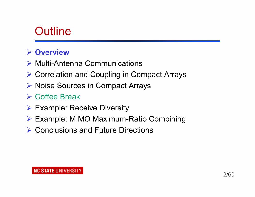
Ø OverviewØ Multi-Antenna CommunicationsØ Correlation and Coupling in Compact ArraysØ Noise Sources in Compact ArraysØ Coffee BreakØ Example: Receive Diversity Ø Example: MIMO Maximum-Ratio CombiningØ Conclusions and Future Directions

3/60
Overview
Ø In recent years, multi-antenna arrays have assumed a central role in wireless communications systems
Ø Antenna arrays canv improve signal-to-noise ratio in wireless links vmitigate co-channel interference v provide spatial diversity to combat signal fadingv enable spatial multiplexing (MIMO)v increase wireless capacity in the presence of rich multipath
Ø Performance advantages often scale with the number of elements, if spaced far enough apart

4/60
Overview
Ø Many transceivers are severely constrained in sizeØ Packing more elements in a fixed space can cause
significant interactions among the elementsv electric fields detected by elements become correlatedv radiation pattern of each element becomes distortedv currents in one element induce voltages across its neighborsv noise in each element may become correlated (internal & external)
Ø These interactions can profoundly impact received power, diversity gain and system capacity
Ø Impact depends on the components of transceiver (array, matching, amplifiers, termination, etc)

5/60
Goals
Ø Seek a systems-level perspective on the design of wireless multi-antenna transceivers
Ø Understand how antennas, matching networks, amplifiers and communications algorithms interact to determine overall system performance
Ø Determine how best to jointly optimize these interacting subsystems
Ø This tutorial talk will focus one particular technique: MIMO maximum-ratio combining (maximum-ratio transmission)
6/60
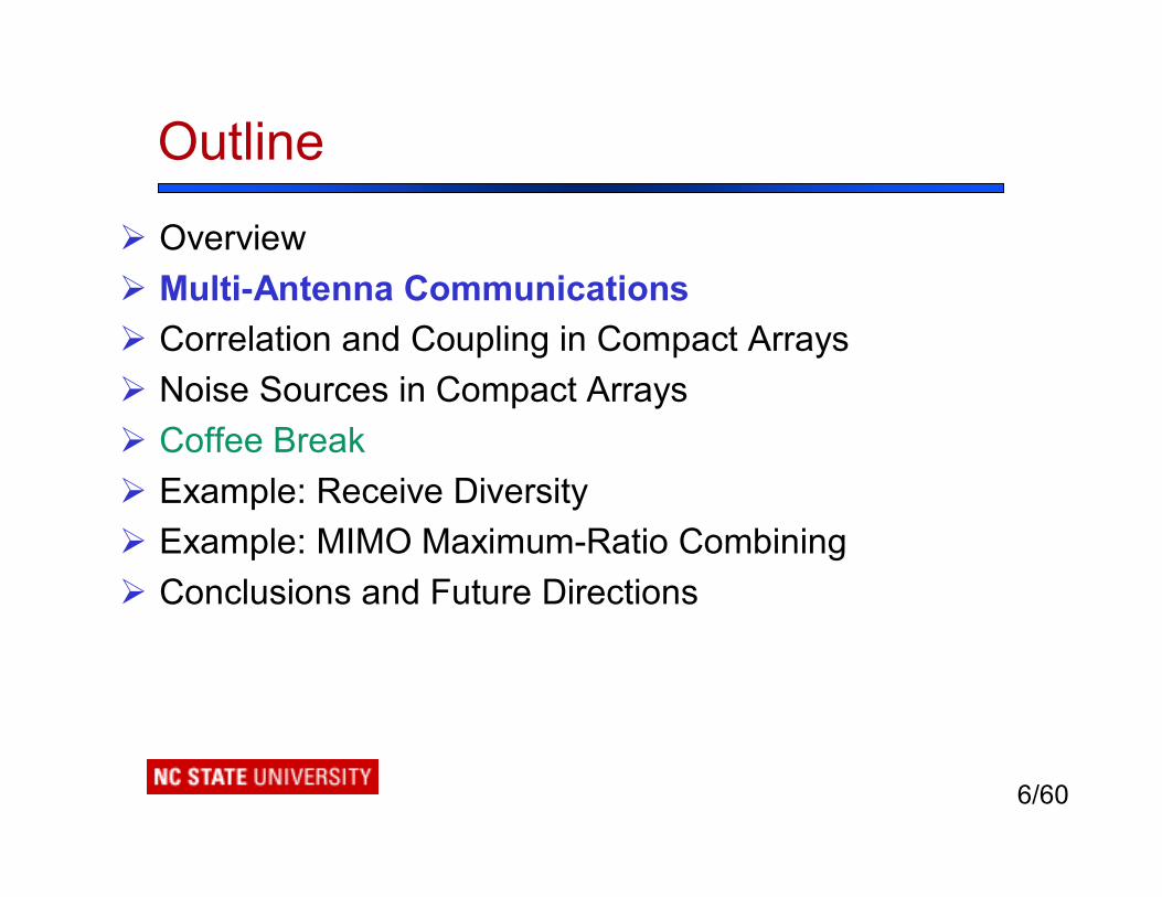
Outline
Ø OverviewØ Multi-Antenna CommunicationsØ Correlation and Coupling in Compact ArraysØ Noise Sources in Compact ArraysØ Coffee BreakØ Example: Receive Diversity Ø Example: MIMO Maximum-Ratio CombiningØ Conclusions and Future Directions

7/60
Multi-Antenna Communications
Ø Wireless signals can propagate to the receiver by many different paths
Ø Constructive and destructive interference of multipaths (and shadowing) results in signal fading
Wireless SignalPropagation
8/60
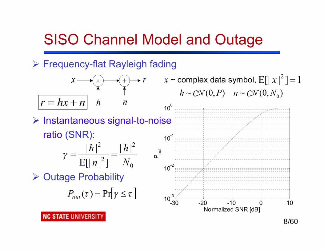
-30 -20 -10 0 1010-3
10-2
10-1
100
Pou
t
Normalized SNR [dB]
SISO Channel Model and OutageØ Frequency-flat Rayleigh fading
Ø Instantaneous signal-to-noise ratio (SNR):
Ø Outage Probability
0~ (0, ) ~ (0, )h P n NCN CNx ~ complex data symbol, 1]|E[| 2 =x
0
2
2
2 ||]|E[|
||Nh
nh
==γ
[ ]τγτ ≤= Pr)(outP
nhxr +=

9/60
Ø Spatial arrays can exploit multipath to improve performanceØ Deploying arrays at both the transmitter and receiver can
dramatically increase wireless capacityØ Multiple-input Multiple-output (MIMO) systems Ø MIMO has quickly moved into recent and emerging
standards (e.g. WCDMA, IEEE 802.11n, 802.16e, 802.20)
MIMO Communications
RxTx Channel
10/60
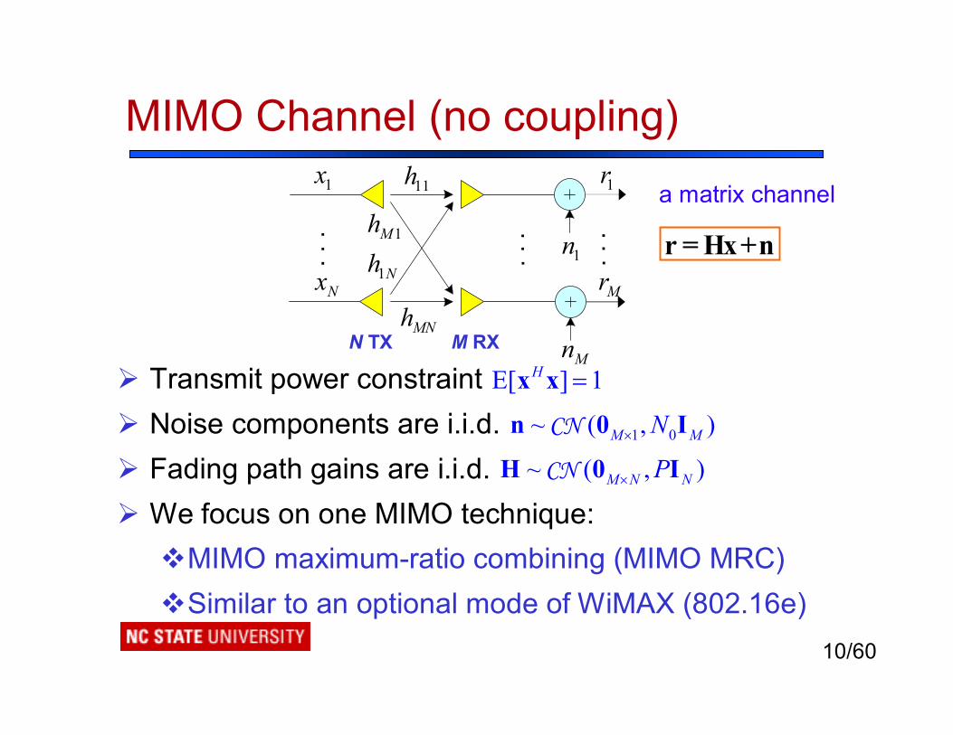
MIMO Channel (no coupling)
Ø Transmit power constraintØ Noise components are i.i.d.Ø Fading path gains are i.i.d.Ø We focus on one MIMO technique: vMIMO maximum-ratio combining (MIMO MRC)vSimilar to an optional mode of WiMAX (802.16e)
r = Hx+n
1 0~ ( , )M MN×n 0 ICN
E[ ] 1H =x xN TX M RX
... .. .
.. .
1x
Nx
1r
Mr1n
Mn
11h
1Mh
1Nh
MNh
a matrix channel
~ ( , )M N NP×H 0 ICN
11/60
Mr
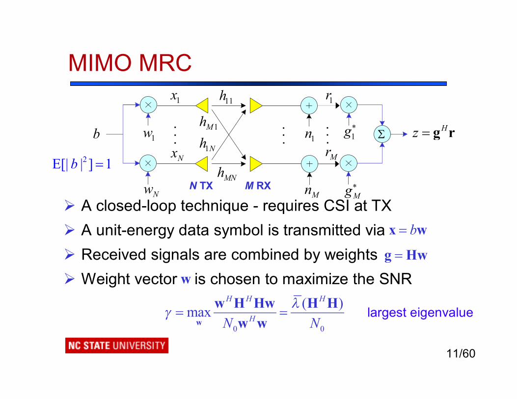
MIMO MRC
Ø A closed-loop technique - requires CSI at TXØ A unit-energy data symbol is transmitted viaØ Received signals are combined by weights Ø Weight vector is chosen to maximize the SNR
N TX M RX..
. .. .
.. .
1x
Nx
1r
1n
Mn
11h
1Mh
1Nh
MNh
1w
Nw
b Σ1g∗
Mg∗
Hz = g r
2E[| | ] 1b =
b=x w
=g Hww
0 0
( )maxH H H
HN Nλγ = =
w
w H Hw H Hw w
largest eigenvalue

12/60
Example: Maximum Ratio Combining
Ø For N=1, equivalent to receive diversity with MRC
19 dBM=4
16 dBM=3
12 dBM=2
Diversity Gain at 1% Outage
-30 -25 -20 -15 -10 -5 0 5 1010
-4
10-3
10-2
10-1
100
M=1
M=2
M=3M=4
Pou
t
Normalized SNR [dB]
MRC provides a large diversity gain
13/60
Outline
Ø OverviewØ Multi-Antenna CommunicationsØ Correlation and Coupling in Compact ArraysØ Noise Sources in Compact ArraysØ Coffee BreakØ Example: Receive Diversity Ø Example: MIMO Maximum-Ratio CombiningØ Conclusions and Future Directions

14/60
Correlation and Coupling
Ø Decreasing inter-element spacing in an array can cause significant interactions among elementsv currents in one element induce voltages across its neighborsv electric fields detected by elements become correlatedv radiation pattern of each element becomes distortedv coupled antennas may not radiate/receive power efficientlyv noise in each branch may become correlated
Ø There is a rich literature on the impact of correlation and mutual coupling on the signal component
Ø By contrast, relatively little attention has been paid to noiseØ Noise often modeled as AWGN regardless of coupling or
the surrounding transceiver design

15/60
Selected Prior Work on Coupling
MC on receive diversity MRCand optimum load network
MC on adaptive arraywith interference
MC on conventional MIMO
Network analysismatching networks
Matching networksBandwidth analysis
Lee (1970) Gupta et al (1983)
Lau & Molisch (2006)Wallace & Jensen (2004)
MC on spatial diversity(V-BLAST/Alamouti scheme)
Clerckx et al (2003)
Noise model
Gans (2006)
Svantesson et al (2001)Janaswamy (2002)

16/60
Mutual Coupling
Ø Current in one antenna induces a voltage across its neighbors
Ø Consider array of half-wavelength dipoles separated by distance
Ø Voltage-current relationship is described by an impedance matrix
Ø How to calculate ?v Thin-dipole approximations (Balanis ’05)v Numerical simulations (NEC)
d
a
ld
11 1
1
N
A
N NN
z z
z z
=
ZL
M O ML
A=V Z I
AZ

17/60
Mutual Coupling
d
a
lijZ R jX= +
coupling can be significant over distances up to several wavelengths

18/60
Receive Array ModelØ Model receive array as M-port Thevenin equivalent network:
~ ( , )Σoo hh 0CNOpen-circuit fadingho1x
. . .
ZA
v1
i1
hoMx
vM
iM
xoA hiZv +=
Signal is not observed directly, but rather is used to drive some device

19/60
vMaximum power delivered to load iff (Hermitian match)v Simpler, suboptimal solution: (Self-matching)
Observed SignalØ Matching network connects array to rest of receiver:
H=in AZ Z( )diag H=in AZ Z
Matching network is lossless
. . .
. . .Observedsignals
20/60
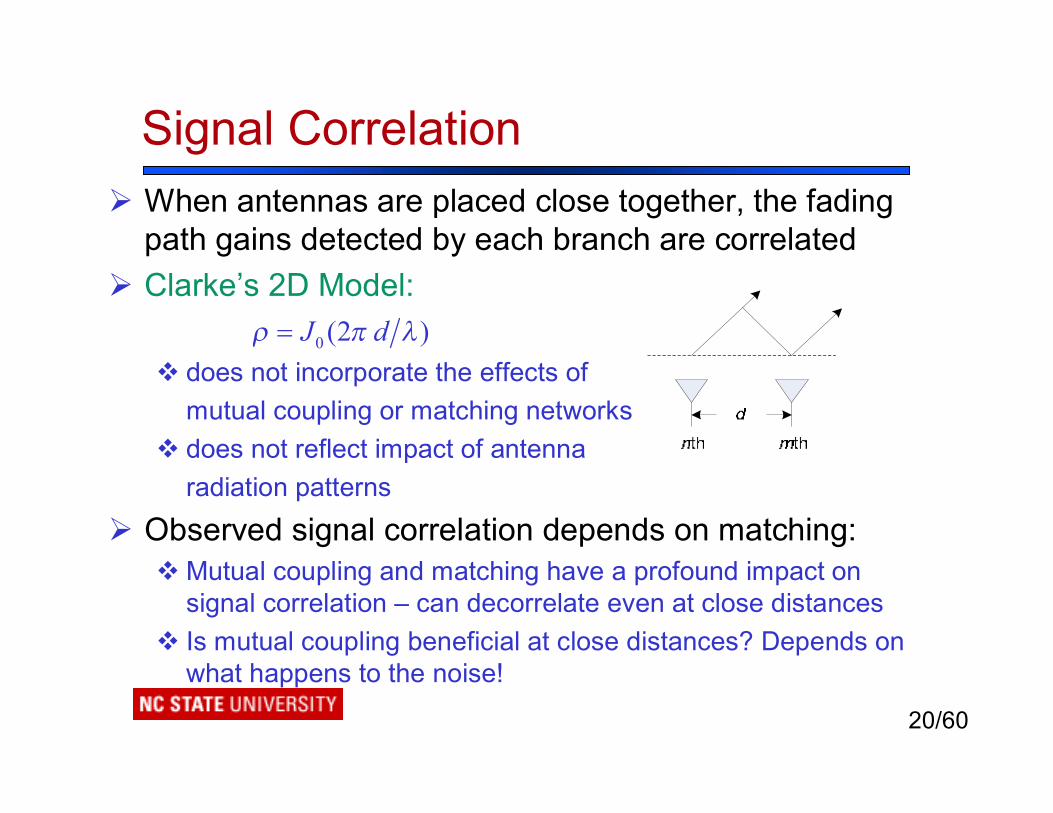
Signal CorrelationØ When antennas are placed close together, the fading
path gains detected by each branch are correlatedØ Clarke’s 2D Model:
v does not incorporate the effects of mutual coupling or matching networks
v does not reflect impact of antennaradiation patterns
Ø Observed signal correlation depends on matching:vMutual coupling and matching have a profound impact on
signal correlation – can decorrelate even at close distancesv Is mutual coupling beneficial at close distances? Depends on
what happens to the noise!
0 (2 )J dρ π λ=
21/60
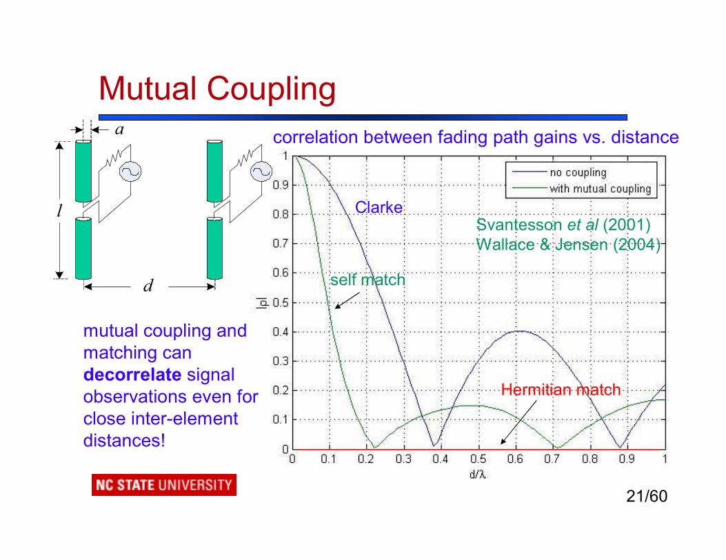
Mutual Coupling
d
a
l
mutual coupling and matching can decorrelate signal observations even for close inter-element distances!
correlation between fading path gains vs. distance
Svantesson et al (2001)Wallace & Jensen (2004)
Clarke
self match
Hermitian match
22/60
Outline
Ø OverviewØ Multi-Antenna CommunicationsØ Correlation and Coupling in Compact ArraysØ Noise Sources in Compact ArraysØ Coffee BreakØ Example: Receive Diversity Ø Example: MIMO Maximum-Ratio CombiningØ Conclusions and Future Directions

23/60
Noise in Compact Arrays
Ø Most studies of compact arrays have not included detailedphysical models of noise
Ø Instead noise is often modeled as AWGN with a fixed distribution, regardless of source or the transceiver design
Ø Real receivers are plagued by diverse noise sourcesØ These sources are affected by coupling, matching and
amplifiers in very different waysØ Since signal and noise play equal roles in most
performance metrics, a model that does not accurately represent noise may not accurately predict performance

24/60
Noise in Compact Arrays
Ø Some recent work uses improved noise models:vMorris-Jensen ‘05: amplifier-noise-limited casev Gans ‘06: sky-noise-limited case
Ø Modern LNAs often have low noise figures, so no single source dominates
Ø Domizioli-Hughes-Gard-Lazzi ‘07:v A receiver model that articulates the main sources of noisev Relates spatial noise correlation to antennas, front-end amplifiers
and matching networkv Optimal receivers and outage probability for MIMO MRC with
receiver coupling

25/60
A Multi-Antenna ReceiverØ Consider a receiver with post-detection combining:
Ø Each stage contributes noise to the outputØ Use noise theory to establish a noise model for each
component, then calculate output noise correlation Σn
Assume coupling in antennas only
26/60
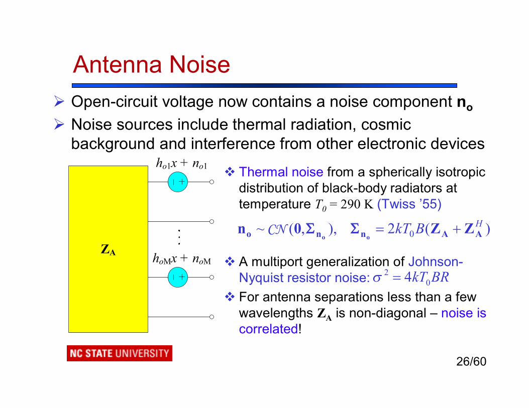
v Thermal noise from a spherically isotropic distribution of black-body radiators at temperature T0 = 290 K (Twiss ’55)
v A multiport generalization of Johnson-Nyquist resistor noise:
v For antenna separations less than a few wavelengths ZA is non-diagonal – noise is correlated!
Antenna NoiseØ Open-circuit voltage now contains a noise component no
Ø Noise sources include thermal radiation, cosmic background and interference from other electronic devices
)(2),,(~ 0HBkT AAnno ZZ0n
oo+=ΣΣCN
ho1x + no1
ZA hoMx + noM2
04kT BRσ =
27/60
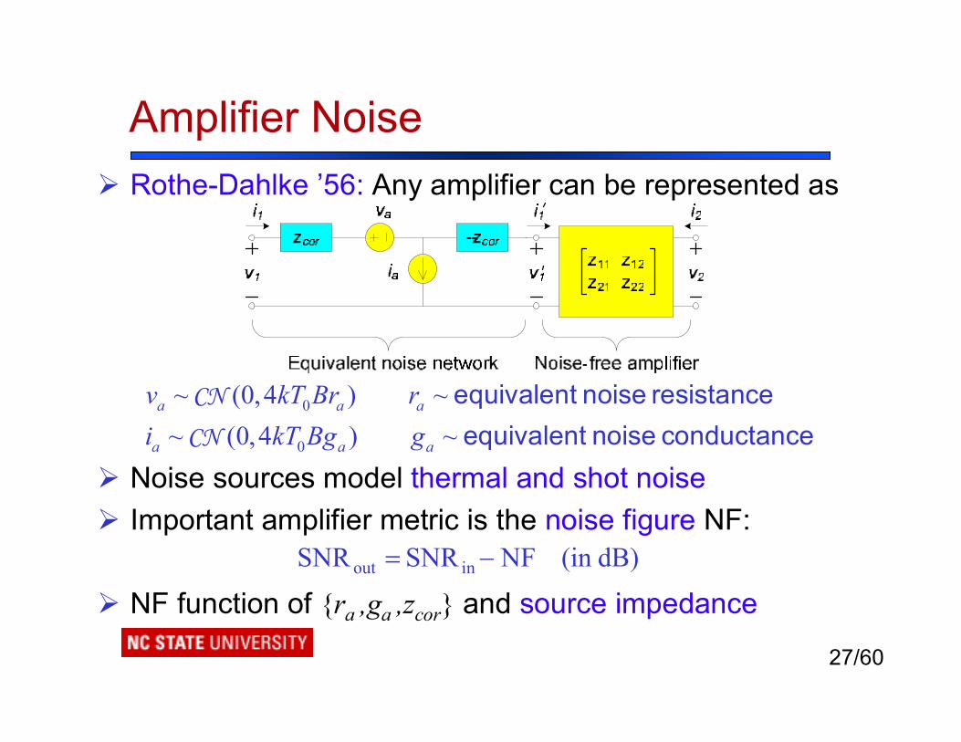
Amplifier NoiseØ Rothe-Dahlke ’56: Any amplifier can be represented as
Ø Noise sources model thermal and shot noiseØ Important amplifier metric is the noise figure NF:
Ø NF function of ra ,ga ,zcor and source impedance
0
0
~ (0,4 ) ~~ (0,4 ) ~
a a a
a a a
v kT Br ri kT Bg g
CN
CN
equivalent noise resistanceequivalent noise conductance
dB)(in NFSNRSNR inout −=

28/60
Downstream NoiseØ The front-end amplifiers may be followed by filters,
mixers, amplifiers and other noisy componentsØ These downstream components tend to be electrically
isolated from other branches and the front-end, but contribute to the overall noise budget
Ø We lump all such contributions into one equivalent noiseterm followed by an equivalent load
)4,0(~ 0 dd BrkTv CNdownstream noise

29/60
A Multi-Antenna Receiver Model
Ø Outage probability of optimal combiner is a function of the eigenvalues of the SNR matrix 1−= nhΣΣΣ
nhvr L +== x
ho1x + no1
. . .
ZA
zcor -zcor
va1
ia1z11 z12z21 z22
zLvL1
vd1
hoMx + noM
zcor -zcor
vaM
iaMz11 z12z21 z22
zLvLM
vdM
Antenna Array Front-End Amplifiers Load. . . . . .
. . .
Lv

30/60
A Multi-Antenna Receiver ModelAntenna Array Matching Network Front-end Amplifiers Load
v Noise figure of amplifiers minimized iff (multiport match)v A simpler, suboptimal solution: Match for isolated dipoles (self-match)
optz=inZ I

31/60
Outline
Ø OverviewØ Multi-Antenna CommunicationsØ Correlation and Coupling in Compact ArraysØ Noise Sources in Compact ArraysØ Coffee BreakØ Example: Receive DiversityØ Example: MIMO Maximum-Ratio CombiningØ Conclusions and Future Directions

32/60
An Example: Receive DiversityØ Consider now an example of correlation at the receiverv For N=1, MIMO MRC reduces to receive diversity with maximum-
ratio combiningv Traditional MRC is not optimal because of the noise correlation
Ø Questions:vWhat is the optimal combiner?v Does mutual coupling and correlation help or hurt performance?v How close can we make the antenna elements and preserve the
benefits of MRC?vWhat impact do different noise sources and matching techniques
have on performance?
33/60
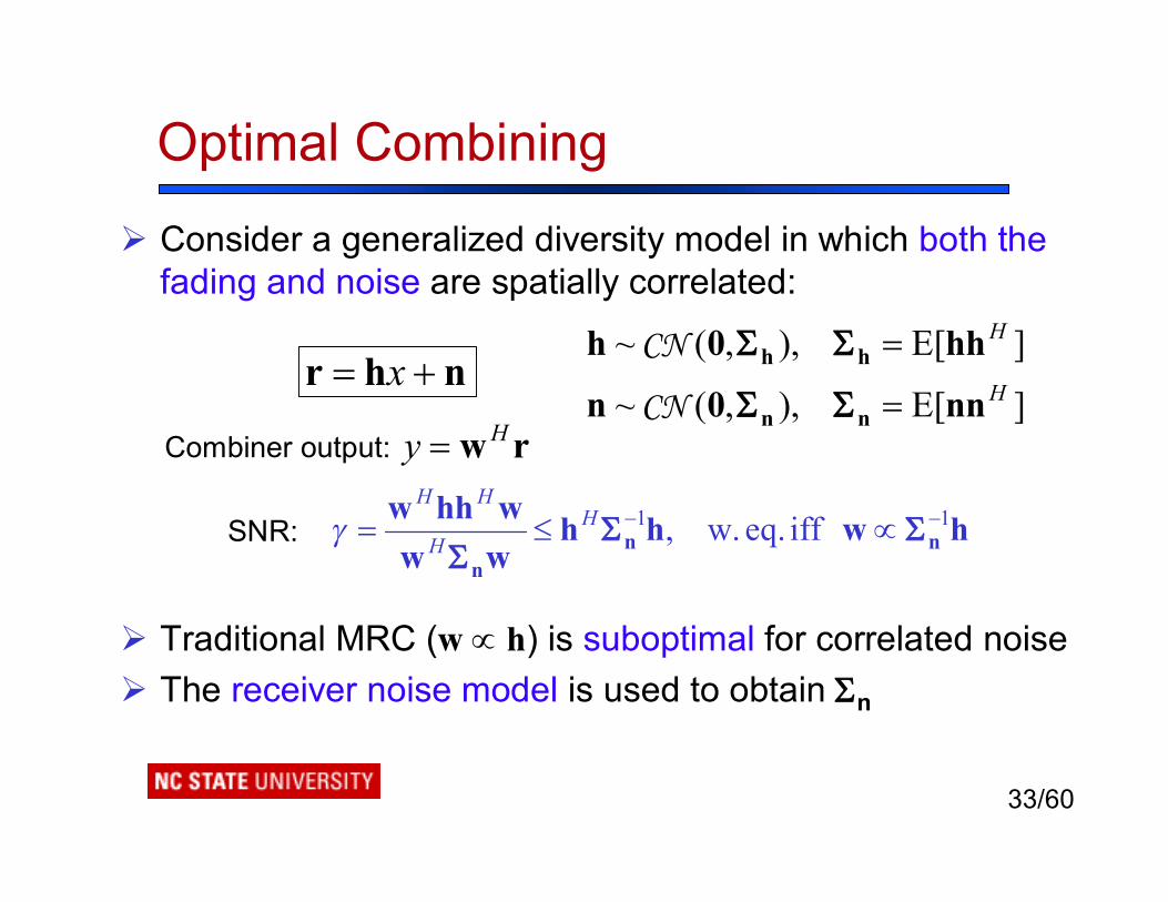
Optimal Combining
Ø Consider a generalized diversity model in which both the fading and noise are spatially correlated:
Ø Traditional MRC (w ∝ h) is suboptimal for correlated noiseØ The receiver noise model is used to obtain Σn
nhr += x]E[),,(~
]E[),,(~H
H
nn0n
hh0h
nn
hh
=
=
ΣΣ
ΣΣ
CN
CN
rw Hy =
hwhhwwwhhw
nnn
11 iff eq. w., −− ∝≤= ΣΣΣ
HH
HH
γ
Combiner output:
SNR:
34/60
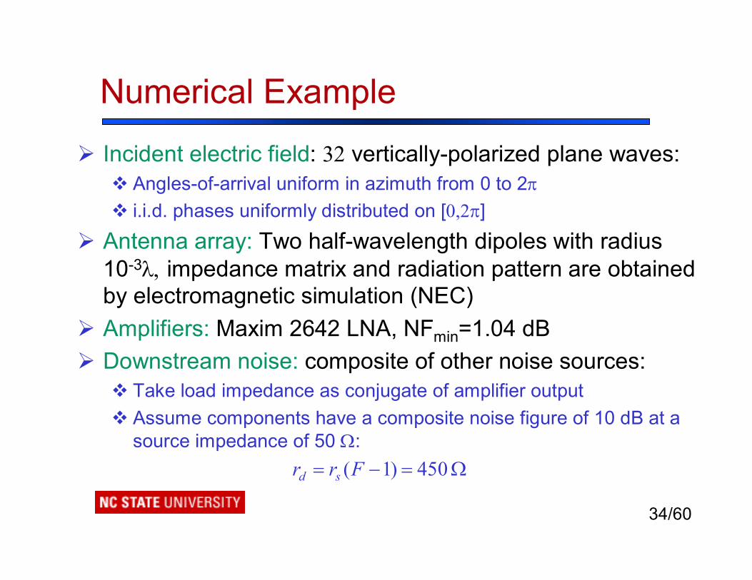
Numerical Example
Ø Incident electric field: 32 vertically-polarized plane waves:v Angles-of-arrival uniform in azimuth from 0 to 2πv i.i.d. phases uniformly distributed on [0,2π]
Ø Antenna array: Two half-wavelength dipoles with radius 10-3λ, impedance matrix and radiation pattern are obtained by electromagnetic simulation (NEC)
Ø Amplifiers: Maxim 2642 LNA, NFmin=1.04 dBØ Downstream noise: composite of other noise sources:v Take load impedance as conjugate of amplifier outputv Assume components have a composite noise figure of 10 dB at a
source impedance of 50 Ω:Ω=−= 450)1(Frr sd

35/60
Impact of Matching, M=2
0 0.2 0.4 0.6 0.8 17
8
9
10
11
12
13
d/λ
Div
ersi
ty G
ain
[dB
]
i.i.d. Fading & NoiseMultiport MatchSelf Match
Diversity gain at 1% outage
36/60
Different Noise Sources (Self Match)
0 0.2 0.4 0.6 0.8 17
8
9
10
11
12
13
d/λ
Div
ersi
ty G
ain
[dB
]
i.i.d. Fading & NoiseAntenna NoiseAmplifier NoiseDownstream Noise
Diversity gain at 1% outage
For multiport matching, performance of all three noise sources coincide
For self matching, performance of three noise sources diverge
37/60
Observations (M=2)Ø Matching has significant impact on diversity gain forvmultiport matching performance is close to i.i.d. at all distancesv self-matching incurs a significant penalty at small distances
Ø Self-matching: sources impact perform in different waysv Antenna thermal noise becomes correlated as the antennas are
brought closer together – the least detrimental noisev Amplifier noise power increases as the antennas are brought closer
together – the most detrimental noisev Downstream noise behaves similar to i.i.d. AWGN – impact is
between that of antenna and amplifier noise
Ø Multiport match: performance doesn’t depend on noise source
Ø Antenna noise: performance does not depend on matching
0.3d λ<

38/60
0 0.2 0.4 0.6 0.8 1-1.5
-1
-0.5
0
0.5
1
1.5
2
2.5
d/λ
Nor
mal
ized
Out
put P
ower
[dB
]SignalAntenna NoiseAmplifier NoiseDownstream Noise
Signal and Noise Power (Self Match)
Observed output power of signal and noise sources relative to M=2 uncoupled antennas
(per
bra
nch)

39/60
Signal and Noise Correlation
0 0.2 0.4 0.6 0.8 10
0.1
0.2
0.3
0.4
0.5
0.6
0.7
0.8
0.9
1
d/λ
Cor
rela
tion
Coe
ff.SignalAntenna NoiseAmplifier NoiseDownstream Noise
40/60
CommentsØ Insights on why amplifier noise is harmful can be gained by
examining the output power due to each noise sourceØ Ideal multiport match may be difficult to realize in practiceØ For small distances, performance of multiport matching
becomes extremely sensitive to any variations in v receiver antenna impedancesv amplifier impedances and noise parametersv downstream noise parametersv carrier frequency and bandwidth (observed for different receiver
model by Lau-Molisch ’05)
Ø At small distances, accurate modeling of the dominant noise sources is critical to predicting and optimizing performance
41/60
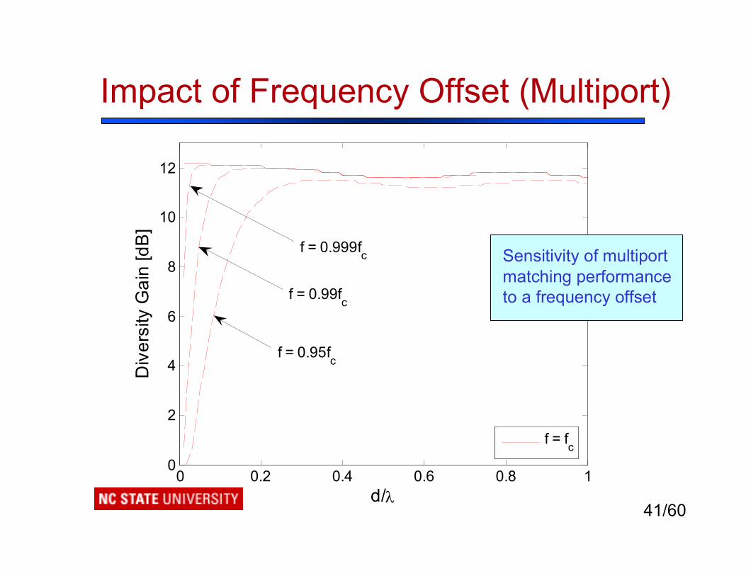
Impact of Frequency Offset (Multiport)
0 0.2 0.4 0.6 0.8 10
2
4
6
8
10
12
d/λ
Div
ersi
ty G
ain
[dB
]
f = fc
f = 0.999fc
f = 0.99fc
f = 0.95fc
Sensitivity of multiportmatching performance to a frequency offset

42/60
Outline
Ø OverviewØ Multi-Antenna CommunicationsØ Correlation and Coupling in Compact ArraysØ Noise Sources in Compact ArraysØ Coffee BreakØ Example: Receive Diversity Ø Example: MIMO Maximum-Ratio CombiningØ Conclusions and Future Directions
43/60
An Example: Transmitter CouplingØ Consider now MIMO MRC with transmitter coupling only v Coupled transmit antennas radiate power less efficientlyv Alters the mathematics of the MIMO MRC optimizationv A different transmission algorithm needed to optimize output SNR
Ø Questions:vWhat is the optimal MIMO MRC transmission algorithm?v Does mutual coupling and correlation help or hurt performance?v How close can we make the antenna elements and preserve the
benefits of MIMO MRC?
Ø Dong-Hughes-Lazzi ‘07:v Considers MIMO MRC with transmit correlation v Optimal transmission algorithms for three different power metricsv Expressions for the outage probabilities

44/60
Selected Prior Work on MIMO MRC
Concept
Optimal Transmissionfor i.i.d. Rayleigh channel
One-sided Correlated Rayleigh Fading Channel
Two-sided Correlated Rayleigh Fading Channel
Lo (1999)
Tse et al (2000) and Dighe et al (2001)
Kang et al (2003) and Zanella et al (2005)
McKay et al (2006)
45/60
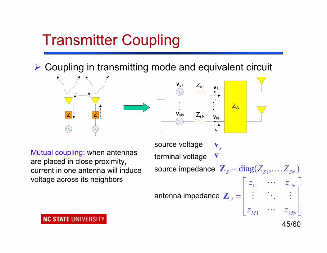
Transmitter Coupling
Ø Coupling in transmitting mode and equivalent circuit
svsource voltageterminal voltage
1diag( , , )S S SNZ Z=Z …
Mutual coupling: when antennas are placed in close proximity, current in one antenna will induce voltage across its neighbors
11 1
1
N
A
M MN
z z
z z
=
ZL
M O ML
source impedance
antenna impedance
v

46/60
A Transmitter ModelØ A lossless matching network is used to efficiently
transfer power to antennas
Ø Hermitian match:Ø Self match: apply same port-by-port conjugate matching
as in the uncoupled case (simpler but suboptimal)
t s=v C vs b=v w
ZS1
.
.
.ZA
vS1
vaN
.
.
.
i
+
-
ZSN
vSN+
-
Matchingnetworks ZM=
Zaa Zab
Zba Zbb+-
ib
+-
+-
vb1
vbN vN+-
va1+-
v1+-
ia
Source voltage:
Terminal voltage:
1 1( ) ( )t A aa A ab S− −= + + inC Z Z Z Z Z Z
Coupling matrix:
HS=inZ Z
inZ

47/60
Transmitter Power MetricsØ Coupled antennas may radiate power less efficientlyØ Several different power metrics have been proposed
Ø Traditional:v power delivered when source connected to bank of 1Ω resistorsv does not correspond to any actual power generated in system
Ø Radiated power:v Power radiated by lossless antennas
Ø Power generated:v Power generated by the sourcev Reflects impact of transmitter matching on performance
12
Hs s sp = v v
11 Re 2
H Ht s s t A tp −= =v Dv D C Z C
(Janaswamy ’02)
11 Re( ) 2
Hg s s Sp −= = +inv Fv F Z Z
(Wallace-Jensen ’04)
(Dong-Hughes-Lazzi ’07)

48/60
System Model
Ø Received signal
Ø MIMO MRC output combiningtb= +r = Hv+n HC w n
Htz hb n= + == g r g HC w% %
Ø Assumptions:v Rich scattering environment with negligible delay spreadvMutual coupling and correlation at TX but not at RX
v Noise is i.i.d. Gaussian2
1~ ( , )M Mσ×n 0 ICN
rows of are ~ ( , )M N× ΣHH 0CN

49/60
(or )
Optimal TransmissionØ We sketch optimal transmission for radiated power
metric only (others are similar)Ø Problem: MIMO MRC seeks to choose w to maximize
subject to a transmit power constraint
Ø Solution:
where
2
2 2
| | 1( )[| | ]
H H Ht t
hE n
γσ
=w = w C H HC w%%
(instantaneous SNR)
11 1 Re 2 2
H H Ht s s t t A tp −= = ≤ Γ =v Dv w Dw D C Z C
maxmax ( )o tt tγ γ= Γ Λ
ww =
maxtΛ is the largest eigenvalue of
1H Ht t
−C H HC D
1/2 ˆ2ot
−= Γ ⋅w D u
1/2 1/2H Ht t
− −D C H HC D(unit-length eigenvector)
50/60
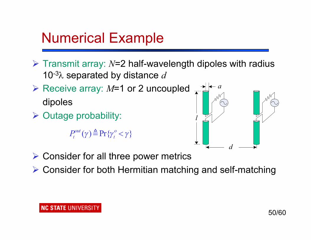
Numerical Example
Ø Transmit array: N=2 half-wavelength dipoles with radius 10-3λ separated by distance d
Ø Receive array: M=1 or 2 uncoupled dipoles
Ø Outage probability:
Ø Consider for all three power metricsØ Consider for both Hermitian matching and self-matching
d
a
l
( ) Pr out ot tP γ γ γ<@

51/60
5 10 15 20 25 3010-3
10-2
10-1
100
γ/Γt [dB]
Ptou
t ( γ)
2×1
2× 2
Analytical (i.i.d.)Analytical (no coupling)Analytical (self-match)Analytical (Herm.-match)Monte-Carlo simulation
Outage Probability vs. SNR
0.3d λ=
(normalized SNR)
fixed distance
2x1
2x2
radiated powermetric
52/60
0.1 0.2 0.3 0.4 0.5 0.6 0.7 0.8 0.910
-4
10-3
10-2
10-1
d/λ
Ptou
t ( γ)
i.i.d.no couplingcoupling, self-matchcoupling, Herm.-match
0.1 0.2 0.3 0.4 0.5 0.6 0.7 0.8 0.910
-4
10-3
10-2
10-1
d/λ
Ptou
t ( γ)
i.i.d.no couplingcoupling, self-matchcoupling, Herm.-match
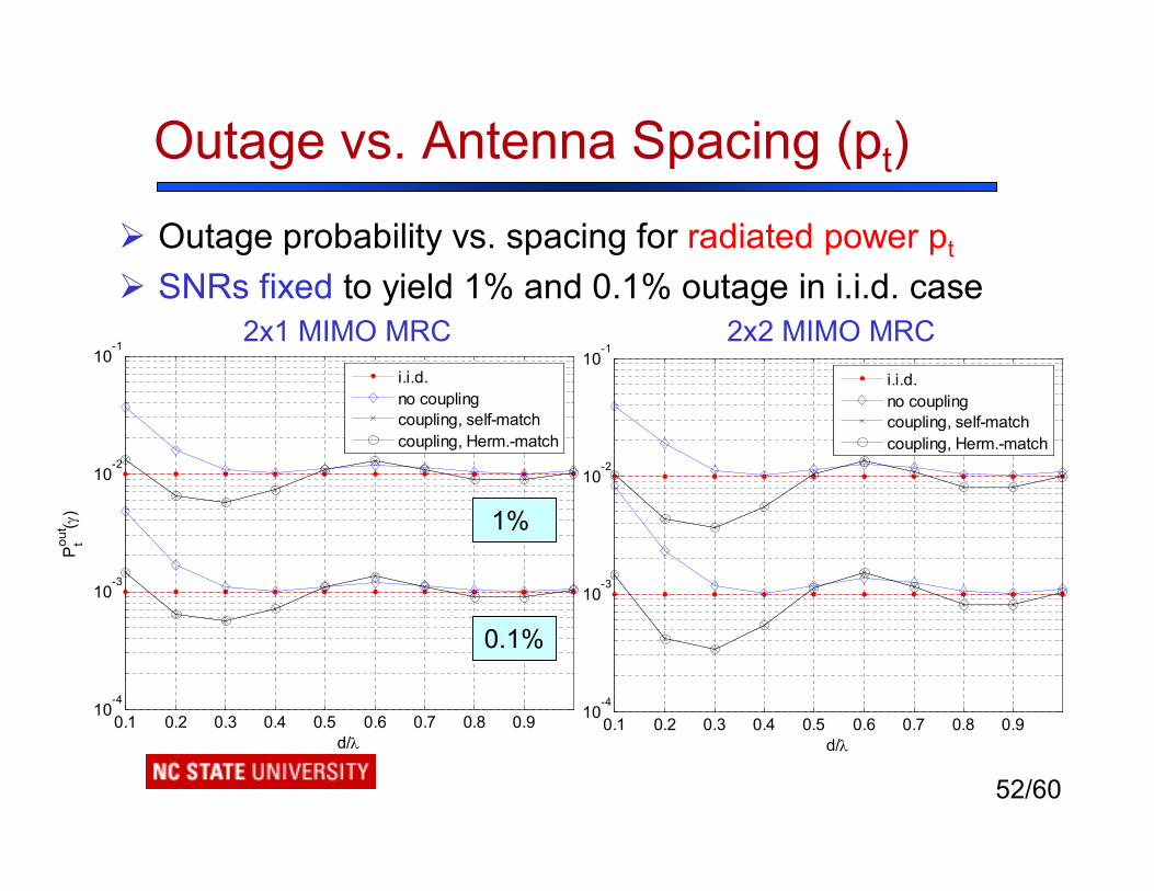
Outage vs. Antenna Spacing (pt)
Ø Outage probability vs. spacing for radiated power pt
Ø SNRs fixed to yield 1% and 0.1% outage in i.i.d. case2x1 MIMO MRC 2x2 MIMO MRC
1%
0.1%

53/60
0.1 0.2 0.3 0.4 0.5 0.6 0.7 0.8 0.910
-4
10-3
10-2
10-1
d/λ
Psou
t ( γ)
i.i.d.no couplingcoupling, self-matchcoupling, Herm.-match
0.1 0.2 0.3 0.4 0.5 0.6 0.7 0.8 0.910
-4
10-3
10-2
10-1
d/λ
Psou
t ( γ)
i.i.d.no couplingcoupling, self-matchcoupling, Herm.-match
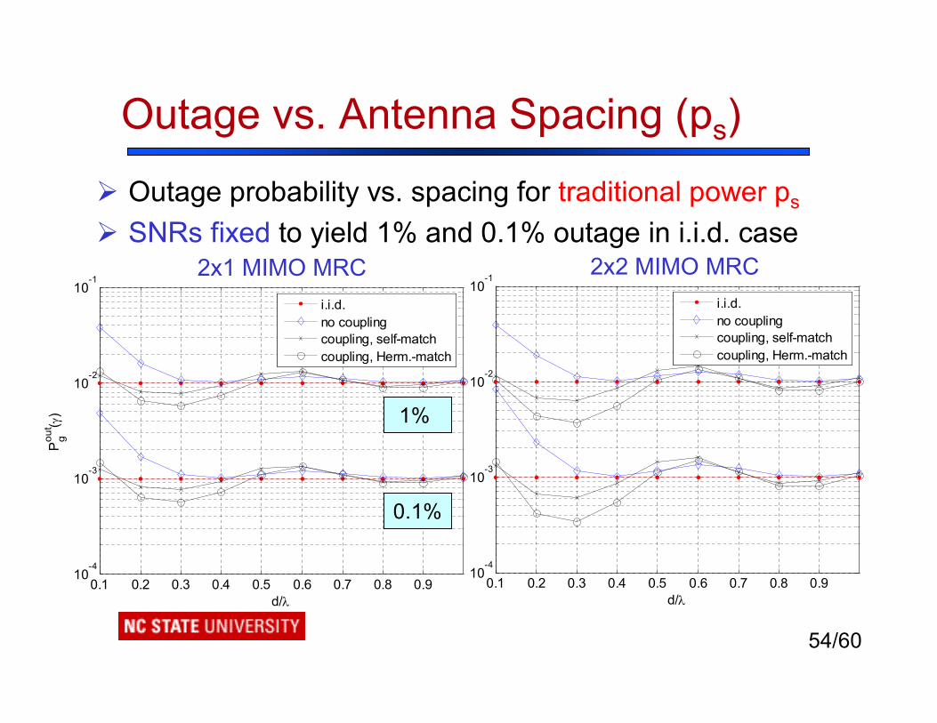
Ø Outage probability vs. spacing for generated power pg
Ø SNRs fixed to yield 1% and 0.1% outage in i.i.d. case2x1 MIMO MRC 2x2 MIMO MRC
1%
0.1%
Outage vs. Antenna Spacing (pg)
54/60
0.1 0.2 0.3 0.4 0.5 0.6 0.7 0.8 0.910
-4
10-3
10-2
10-1
d/λ
Pgou
t ( γ)
i.i.d.no couplingcoupling, self-matchcoupling, Herm.-match
0.1 0.2 0.3 0.4 0.5 0.6 0.7 0.8 0.910
-4
10-3
10-2
10-1
d/λ
Pgou
t ( γ)
i.i.d.no couplingcoupling, self-matchcoupling, Herm.-match
Ø Outage probability vs. spacing for traditional power ps
Ø SNRs fixed to yield 1% and 0.1% outage in i.i.d. case
Outage vs. Antenna Spacing (ps)
2x1 MIMO MRC 2x2 MIMO MRC
1%
0.1%

55/60
Observations (N=2)Ø For coupling tends to improve performance
relative to no-coupling case for radiated power metricv 2-2.5dB for for both Hermitian match and self matchv self-matching incurs a significant penalty at small distances for
other power metrics
Ø For all power metrics best performance is nearv For radiated power, matching has no impact on performancev For generated power, Hermitian match significantly outperforms
self match for
Ø Most of the performance benefits of MIMO MRC can be obtained with antennas spaced apart
0.2 0.45dλ λ≤ ≤
0.2 0.3λ λ−
0.3d λ=
0.3d λ=
0.3d λ≤

56/60
Outline
Ø OverviewØ Multi-Antenna CommunicationsØ Correlation and Coupling in Compact ArraysØ Noise Sources in Compact ArraysØ Coffee BreakØ Example: Receive Diversity Ø Example: MIMO Maximum-Ratio CombiningØ Conclusions and Future Directions
57/60
ConclusionsØ Packing elements close together in an array can cause
significant interactions among the elementsØ These interactions can profoundly impact received
power and diversity gainØ In general, both the signal and noise components of the
receive branches may be correlatedØ Accurate modeling of dominant noise sources is critical
to predicting performance in a multiple-antenna receiverØ Presented receiver model that articulates the main
sources of noiseØ Considered the impact of transmit and receive coupling
on MIMO MRC systems
58/60
ConclusionsØ Derived optimal transmission strategies for MIMO MRC
with transmit and receive couplingØ Results suggest that different noise sources can impact
performance in profoundly different waysØ Multiport matching can significantly outperform self
matching for closely spaced arraysØ Performance of multiport matching for close spacings is
extremely sensitive to antenna and amplifier impedances and noise parameters
Ø All results suggest that most of the performance of MIMO MRC systems can be obtained with arrays of antennas spaced apart 0.2 0.3λ λ−
59/60
Future DirectionsØ Limited feedback for MIMO MRC with mutual couplingv Design criterion for deterministic/adaptive codebooksv Coupling effect on feedback quantization
Ø Mutual coupling effect on multiuser MIMO MRCv Spatial diversity v.s. multiuser diversityv Co-cell and multi-cell interference
Ø Impact of mutual coupling on spatial multiplexingv Fundamental tradeoff between diversity and multiplexingv Pre-coding of data streams
Ø More robust matching techniquesv Optimal matching over a finite bandwidthvMatching for specific communications performance metrics

QUESTIONS?

1
Fundamentals of Networking Lab
802.11 Wireless LANs: State-of-Art
Sumit RoyU. Washington, [email protected]
www.ee.washington.edu/research/funlab

2
Fundamentals of Networking Lab
Pt. I: Status of WLANs
802.11 Review: Architecture, Protocols, Performance
Pt. II: Status of WLANsChallenges for Next Generation WLANsWide-Area Broadband Access with QoS- Emerging Network Architectures- Network Scalability with QoS
3
Fundamentals of Networking Lab
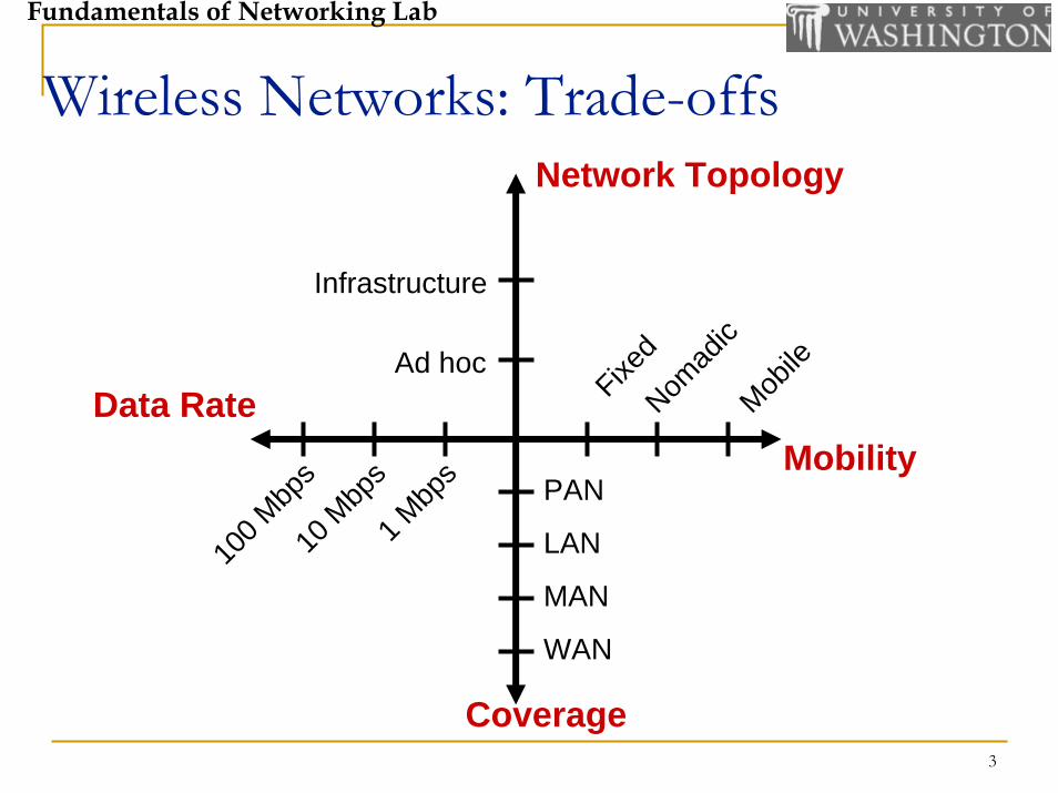
Wireless Networks: Trade-offs
Mobility
Network Topology
Coverage
Ad hoc
Infrastructure
100 M
bps
Nomad
ic
Fixed
10 M
bps
1 Mbp
s PAN
LAN
MAN
WAN
Mobile
Data Rate
4
Fundamentals of Networking Lab
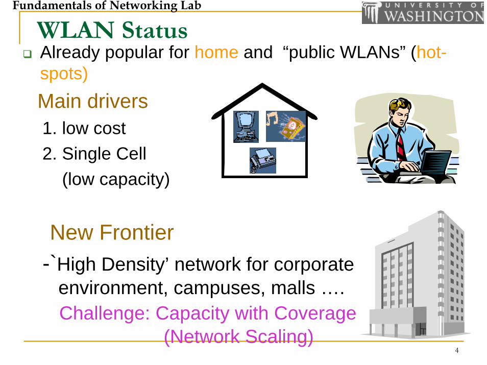
WLAN StatusAlready popular for home and “public WLANs” (hot-spots)Main drivers1. low cost 2. Single Cell
(low capacity)
New Frontier-`High Density’ network for corporate
environment, campuses, malls ….Challenge: Capacity with Coverage
(Network Scaling)
5
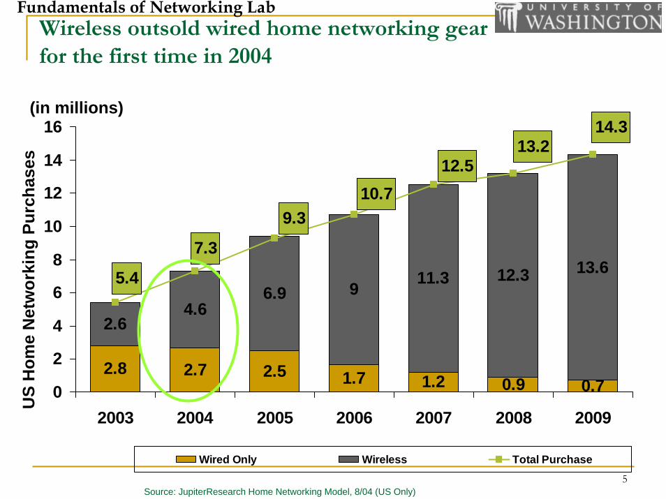
Fundamentals of Networking LabWireless outsold wired home networking gear for the first time in 2004
2.8 2.7 2.5 1.7 1.2 0.7
2.64.6
6.9 9 11.3 12.3 13.6
0.9
14.3
10.712.5
13.2
9.3
5.4
7.3
0
2
4
6
8
10
12
14
16
2003 2004 2005 2006 2007 2008 2009
Wired Only Wireless Total Purchase
US
Hom
e N
etw
orki
ng P
urch
ases
(in millions)
Source: JupiterResearch Home Networking Model, 8/04 (US Only)

6
Fundamentals of Networking Lab
Unlicensed Spectrum OverviewUnlicensed Spectrum Overview
2.4-2.5 GHz 5.1-5.2 GHz 5.2-5.3 GHz 5.7-5.8 GHz
802.11b/gBlueToothHomeRF
802.11a/g 802.11a/g 802.11a/g
Spectral Characteristics Higher FrequenciesLower Frequencies
Transmit Distance / Transmit PowerGreater Less
Multi-Path FadingGreater Less
7
Fundamentals of Networking Lab
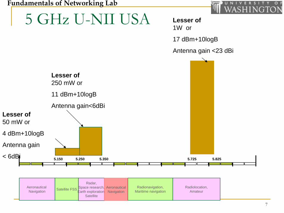
5 GHz U-NII USA
Lesser of50 mW or
4 dBm+10logB
Antenna gain
< 6dBi 5.150 5.250 5.350 5.725 5.825
Lesser of 250 mW or
11 dBm+10logB
Antenna gain<6dBi
Lesser of 1W or
17 dBm+10logB
Antenna gain <23 dBi
Satellite FSSAeronautical Navigation
Radionavigation,Maritime navigation
Radiolocation,Amateur
Radar,Space research,
Earth exploration Satellite
AeronauticalNavigation

8
Fundamentals of Networking Lab
802.11 Standards
802.11b – CCK modulation, upto 11mbps (2.4 GHz), 3 channels802.11g – OFDM (2.4 GHz) upto 54 Mbps, 3 channels802.11a – OFDM (5 GHz) upto 54 Mbps and 8-12 usable channels. 802.11n – OFDM using multiple antenna (MIMO) upto 600mbps, backward compatible 802.11s – Extended Service Set supporting Layer 2.5 MESH

9
Fundamentals of Networking Lab
802.11a Rates
1101
RateBits
1111010101111001101100010011
6
Rate(Mbps)
9121824364854
BPSK
Modulation
BPSKQPSKQPSK
16QAM16QAM64QAM64QAM
R = 1/2
CodingRate
R = 3/4R = 1/2R = 3/4R = 1/2R = 3/4R = 2/3R = 3/4 op
tiona
l
10
Fundamentals of Networking Lab
11
11
11
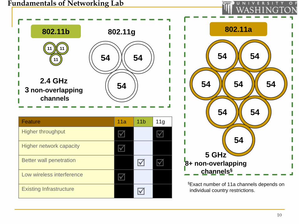
802.11b
54
54
54
2.4 GHz3 non-overlapping
channels
802.11g 802.11a
5 GHz8+ non-overlapping
channels§
5454
54
54
54 54
54
54
Feature 11a 11b 11g
Higher throughput
Higher network capacity
Better wall penetration
Low wireless interference
Existing Infrastructure§Exact number of 11a channels depends on individual country restrictions.

11
Fundamentals of Networking Lab
IEEE 802.11 Operational Modes
Infrastructure Mode : 1-Hop network
Ad Hoc Mode (Independent BSS)
Fundamentals of Networking Lab
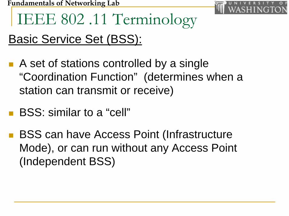
IEEE 802 .11 TerminologyBasic Service Set (BSS):
A set of stations controlled by a single “Coordination Function” (determines when a station can transmit or receive)
BSS: similar to a “cell”
BSS can have Access Point (Infrastructure Mode), or can run without any Access Point (Independent BSS)
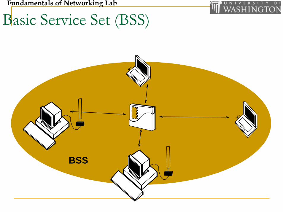
Fundamentals of Networking Lab
Basic Service Set (BSS)
BSS
Fundamentals of Networking Lab
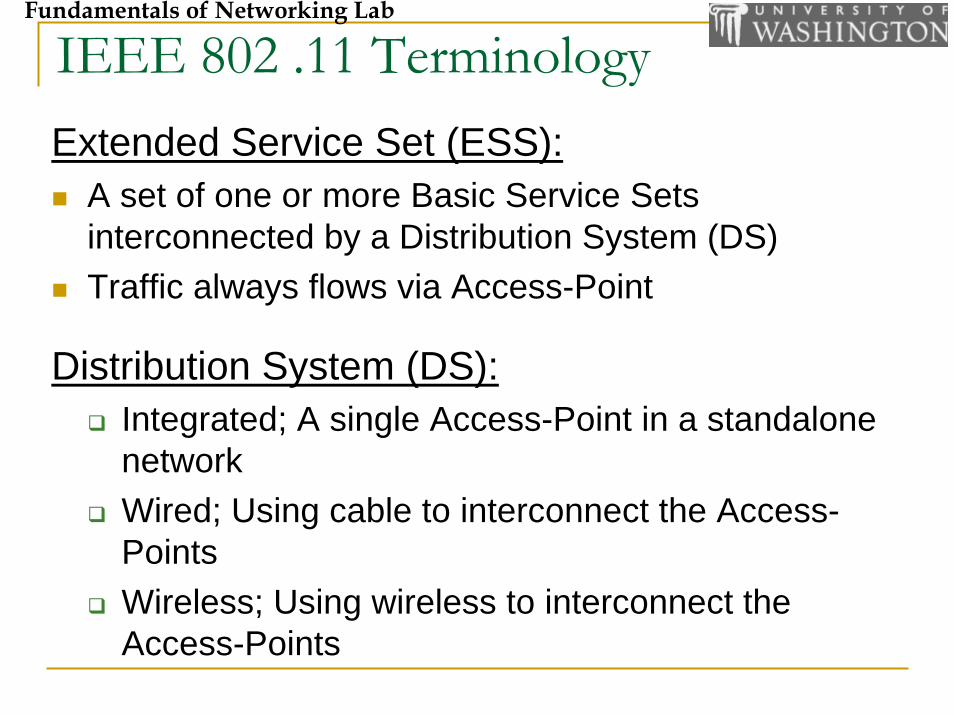
IEEE 802 .11 TerminologyExtended Service Set (ESS):
A set of one or more Basic Service Sets interconnected by a Distribution System (DS)Traffic always flows via Access-Point
Distribution System (DS):Integrated; A single Access-Point in a standalone networkWired; Using cable to interconnect the Access-PointsWireless; Using wireless to interconnect the Access-Points

15
Fundamentals of Networking Lab
Current ESS environment
Wired DS

Fundamentals of Networking Lab
Future: Wireless Distribution System (DS)
BSS
BSS
Distribution
System
17
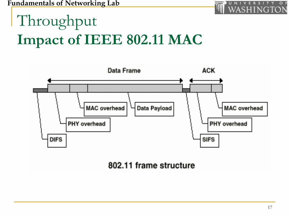
Fundamentals of Networking Lab
ThroughputImpact of IEEE 802.11 MAC

18
Fundamentals of Networking Lab
ThroughputImpact of IEEE 802.11 MAC
19
Fundamentals of Networking Lab
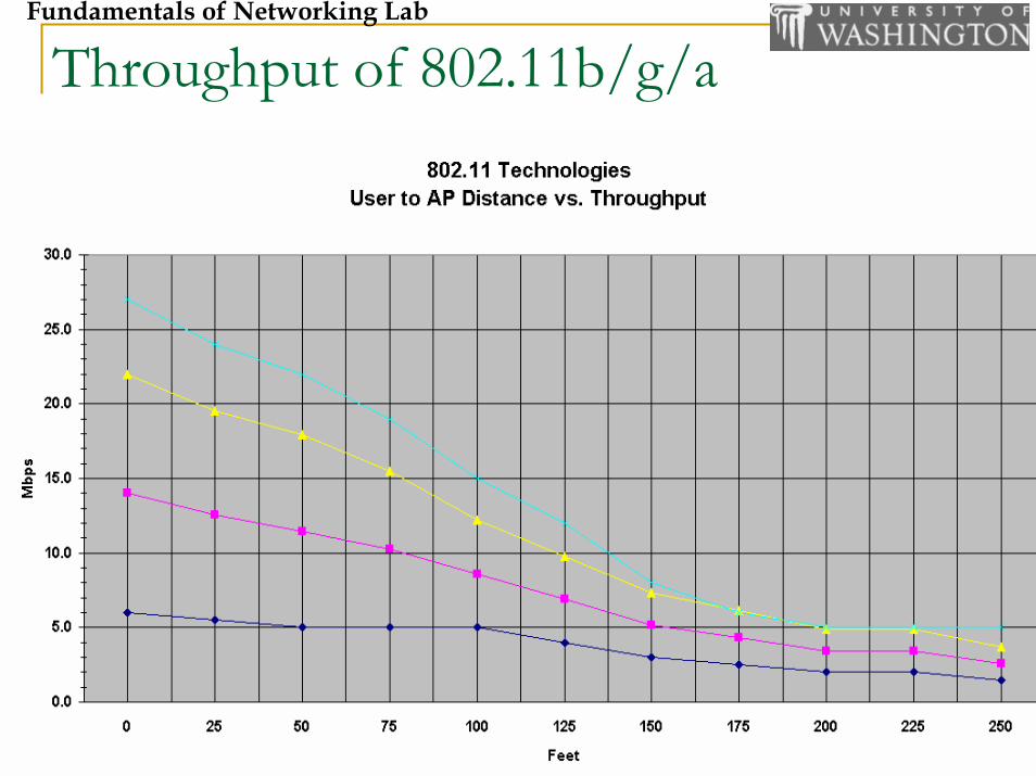
Throughput of 802.11b/g/a
Fundamentals of Networking Lab
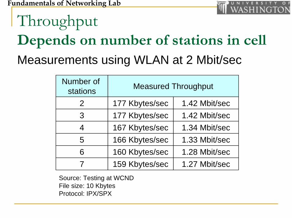
ThroughputDepends on number of stations in cell Measurements using WLAN at 2 Mbit/sec
Number of stations Measured Throughput
2 177 Kbytes/sec 1.42 Mbit/sec3 177 Kbytes/sec 1.42 Mbit/sec4 167 Kbytes/sec 1.34 Mbit/sec5 166 Kbytes/sec 1.33 Mbit/sec6 160 Kbytes/sec 1.28 Mbit/sec7 159 Kbytes/sec 1.27 Mbit/sec
Source: Testing at WCNDFile size: 10 KbytesProtocol: IPX/SPX

21
Fundamentals of Networking Lab
Network Optimization: Today

22
Fundamentals of Networking Lab
AP Positioning
Maximizing coverage (figure on the left)Stations split between 11Mpbs and 5.5Mbps
Maximizing throughput (figure on the right)Nearly all stations are within 11Mbps range
5.5 Mbps11 Mbps

23
Fundamentals of Networking Lab
Load Balancing
AP1 has much greater load than AP2Load could be more balanced by moving the Purple stars to AP2
On the fringe of both networksImprove AP1’s throughput while only slightly decreasing that of AP2
11Mbps
5.5 Mbps
11Mbps
5.5 Mbps
AP 1 AP 2

24
Fundamentals of Networking Lab
Transmit Power
Maximize RSSIHigher signal power, data rateDecrease probability of error
Co-channel interferenceTwo APs transmit on the same channelTheir transmission interfere with each other causing errors, hence retransmission needed
Need to balance transmit power such that RSSI is maximized and co-channel interference is minimized
25
Fundamentals of Networking Lab
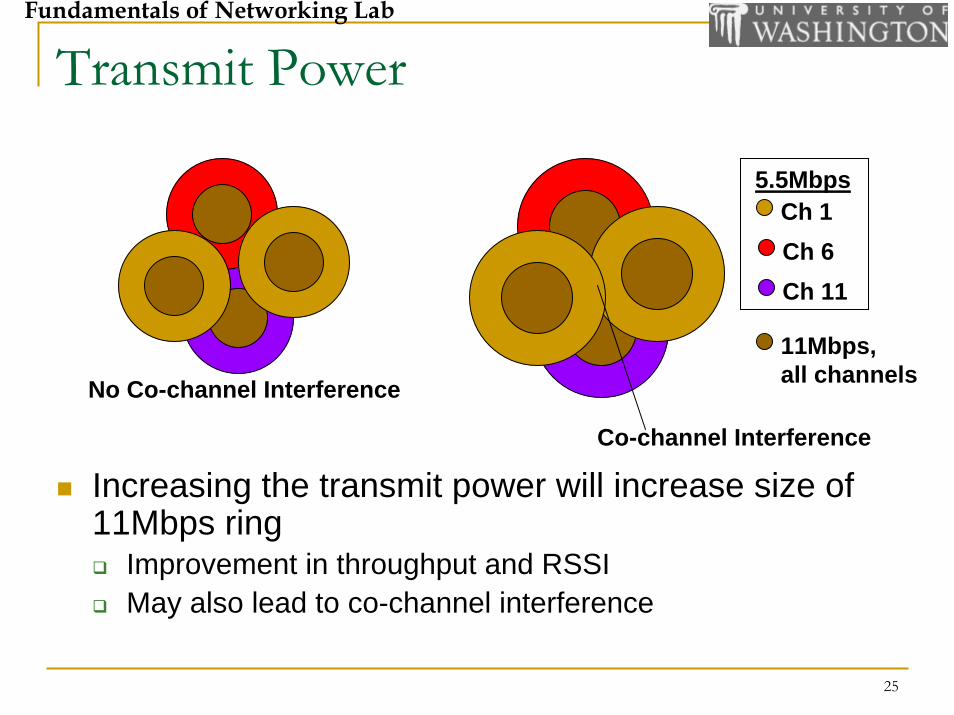
Transmit Power
Increasing the transmit power will increase size of 11Mbps ring
Improvement in throughput and RSSIMay also lead to co-channel interference
Ch 1Ch 6Ch 11
11Mbps, all channels
5.5Mbps
Co-channel Interference
No Co-channel Interference

26
Fundamentals of Networking Lab
Evolution
27
Fundamentals of Networking Lab
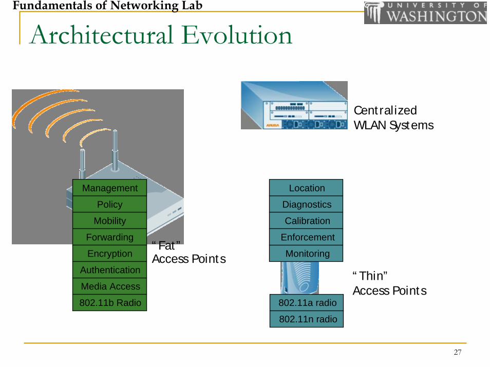
Architectural Evolution
Media Access
802.11b Radio
Policy
Mobility
Forwarding
Encryption
Authentication
Management
“Thin”Access Points
Centralized WLAN Systems
“Fat”Access Points
Diagnostics
Calibration
Monitoring
Enforcement
Location
802.11a radio
802.11n radio

28
Fundamentals of Networking Lab
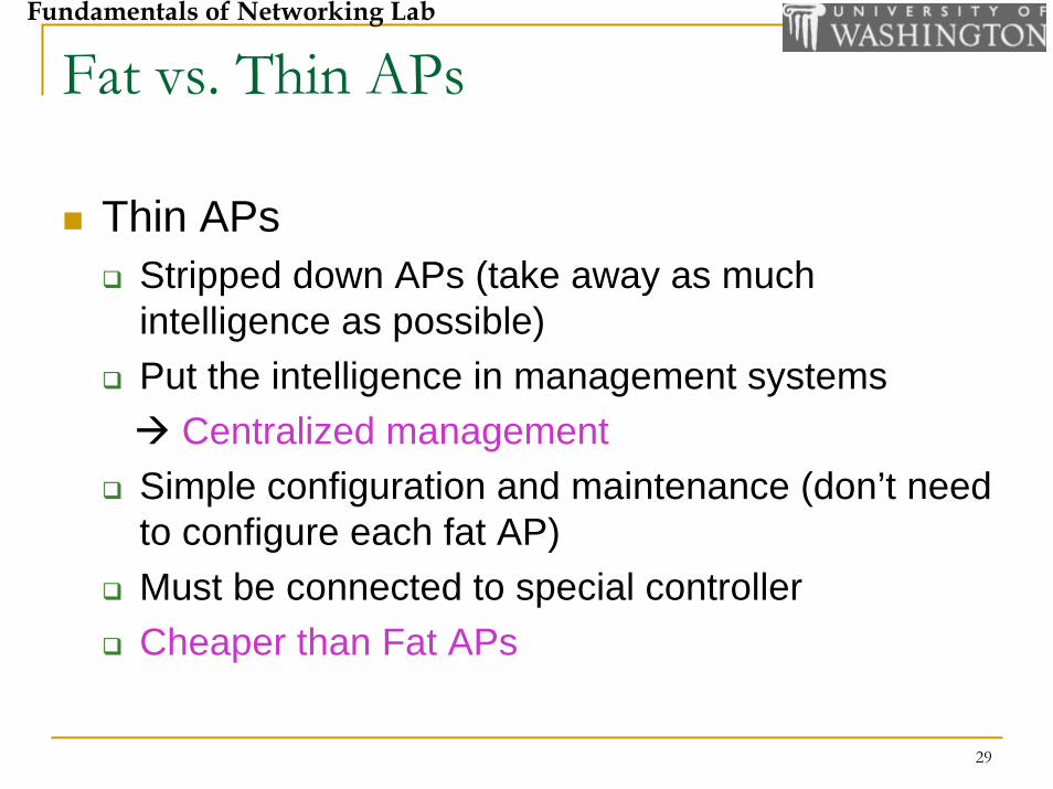
Fat vs. Thin APs
29
Fundamentals of Networking Lab
Fat vs. Thin APs
Thin APsStripped down APs (take away as much intelligence as possible)Put the intelligence in management systems
Centralized managementSimple configuration and maintenance (don’t need to configure each fat AP)Must be connected to special controllerCheaper than Fat APs

30
Fundamentals of Networking Lab
Example: Apartment Block Scenario1 MPEG4 Video Stream: 4 Mbps1 user per 15*15*15 m^3Each AP range is 50 m volume = 4*(50)^3Link Overhead: 20%Required Capacity per cell = 4*1.2*108 Mbs
= 540 Mbps
10 fold improvement required over .11a max rates !!

31
Fundamentals of Networking Lab
Better spectrum usageBetter spectrum usageImproved Link adaptationImproved Link adaptationMore efficient MACMore efficient MACMIMO MIMO
Better spectrum managementBetter spectrum managementCooperative networksCooperative networksNetwork Level AdaptationNetwork Level Adaptation
Greater frequency reuseGreater frequency reuseSmart antennas for interference mitigationSmart antennas for interference mitigationIntelligent MAC and routing Intelligent MAC and routing
How to Solve the Capacity Problem?

Fundamentals of Networking Lab
802.11 High Density Mesh Networks: 802.11 High Density Mesh Networks: Management Principles Management Principles
Sumit RoyUniv. of Washington
Seattle, [email protected]
www.ee.washington.edu/research/funlab
33
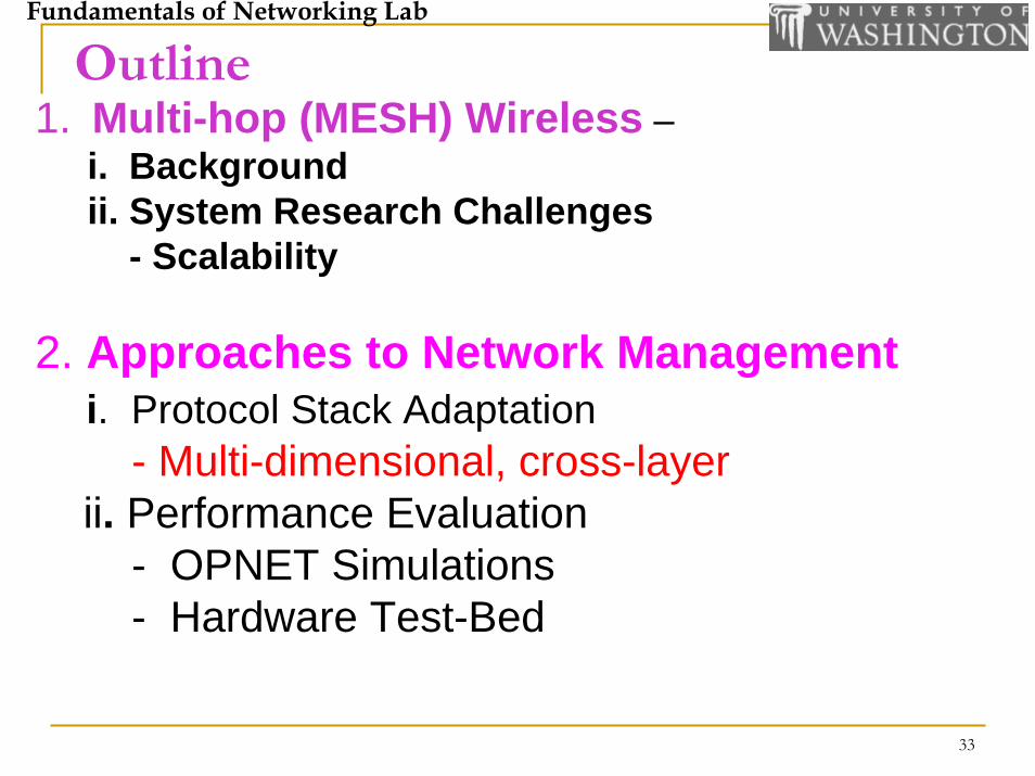
Fundamentals of Networking Lab
Outline1. Multi-hop (MESH) Wireless –
i. Background ii. System Research Challenges
- Scalability
2. Approaches to Network Managementi. Protocol Stack Adaptation
- Multi-dimensional, cross-layerii. Performance Evaluation
- OPNET Simulations- Hardware Test-Bed

34
Fundamentals of Networking Lab
WHY MESH (= Multi Hop)?Cost-effective solution to broadband wireless access Multi-hop network using cheap router nodes
network size vs. transmission distancesmaller hops: higher link rates and power efficiency
potential for improved spatial reuse (higher aggregatenetwork throughput)

35
Fundamentals of Networking Lab
Current StatusInfrastructure Ad Hoc
Single-Hop Wireless LAN, Cellular, etc.
?
Multi-Hop ? Of current interest
• No wireless inter-AP connectivity standard as yet (.11s : nearing completion)• New Layer 2.5 definitions for routing
Only a fraction of mesh nodes are IP-addressibleLayer 2 routing !

36
Fundamentals of Networking Lab
802.11 Mesh ArchitecturesInfrastructure Mode ESS MeshInfrastructure Mode ESS Meshwith WDS Backhaulwith WDS Backhaul
WDS Links
Ad Hoc Links
PeerPeer--toto--Peer Client MeshPeer Client Mesh(Ad Hoc Mode)(Ad Hoc Mode)
Ad Hoc Links
Ad Hoc or WDS Links
Hybrid Infrastructure/Hybrid Infrastructure/Ad Hoc MeshAd Hoc Mesh

37
Fundamentals of Networking Lab
2-Radio AP Mesh NetworksOnly a fraction of mesh points are gateways (hardwired); majority are `soft routers’ cost-effective architecture for scalingEach mesh point has 2 radios: .11 a/b/g(incremental radio cost)AP Mesh on .11a (higher capacity)Client-to-AP on .11bno mutual interferencebetween backhaul and access

38
Fundamentals of Networking Lab
High Density .11 MESH: Challenges
802.11 MAC protocol supports 1-hop (not multi-hop) design for `coverage’ (homes), not QoSHigh Density WLANs
Interference Limited (In-cell `collisions’ and out-of-cellco-channel interference)
Frequency Planning (of limited effect in ad-hoc networks)Investigate other strategies to reduce cell-size (increase spatial re-use) while providing coverage
need a cost-effective multi-hop architecture! Only a subset of Tier-2 mesh nodes are gateways (connected to backbone), most are cheap `soft’ routers.

39
Fundamentals of Networking Lab

40
Fundamentals of Networking Lab
Architecture : Infrastructure
3rd Generation WLAN Infrastructure (Aruba)

41
Fundamentals of Networking Lab
Traditional Fat AP Architecture Full Layer 1/2
functionality including security, roamingBackhaul connection to Ethernet switch
wired Distributionsystem
Mix `n Match APs from different vendors but each AP needs to be configured, does notscale

42
Fundamentals of Networking Lab
Switch Based Thin AP Architecture Thin APs only layer 1 +
min. layer 2 functionsRF controller/wireless switch for centralized management (each controls ~ 100 APs)+Simpler management(don’t need to configure each AP)- No inter-op; needs RF switch + APs from same vendor

43
Fundamentals of Networking Lab
HD WLANs: The Case for Network Management
Design for QoS : driver for high-density WLAN environmentsArchitectural trends (RF Switches with `thin’
APs) provide context/constraint on solutionscurrent solutions are centralized; need for a
better mix of distributed and centralized algorithms !Cross-Layer Adaptation: Layer 1-3 parameters
multi-dimensional network optimization !!

44
Fundamentals of Networking Lab
Cross-Layer Interference Management
• Network ADAPTATION6 Key Parameters (Layers 1-3)
- Txmit Power, CCA Threshold, Link Rate, Receiver Sensitivity
- Contention Window, Interface*- to- Channel Assignment (*multiple interfaces per node)
- Link-aware Routing metrics

45
Fundamentals of Networking Lab
Scaling in Dense Mesh
Typical Solution: increase MESH AP density(i.e. deploy more access points/area)However, with limited # orthogonal channels
more co-channel interferenceOnly link capacity scaling is insufficient for increasing network throughput
MAC overhead typically increases as link rate improves (classical contradiction!)
Wireless networks are moving to THIN protocol stacks (traditional OSI boundaries are being erased); renewed emphasis on layers 1 & 2
cross-layer optimization!

46
Fundamentals of Networking Lab
Cross- Layer Interference Mitigationi. Coding, Beamforming (Physical Layer)ii. Multiple Access Protocol (Layer 2)
- Transmit Power, CCA, rate: MAC driven link-layer parameter adaptation- Contention Window: MAC-layer parameter iii. Link-aware Routing Metric (Layer 3)iv. Radio resource allocation [Multi-Radio]
- Channel-to-(Link, Radio) assignment

47
Fundamentals of Networking Lab
Link Capacity
PHY Optimization: Adaptive Link Layer (Coded Modulation, MIMO …)
MAC Optimization, Channel Allocation
MESH Scaling
Network Throughput
= f Spatial Reuse
Radio Resource Allocation
Multi-radio Utilization,Link-to-radio assignments
xx

48
Fundamentals of Networking Lab
Single Radio Mesh
In single radio, single channel 1-hop networks, Throughput/node typically ~ O(1/na) [a: depends on topology, traffic ..]n: number of nodes in 1-hop radiuse.g. linear chain throughput O(1/n)With multiple (C) channels: Throughput/node ~ O(C/n) due to improved spatial reuse of C channels [better interference management]But End2End Delay: lower bounded by channel switching (turnaround time of transceiver due to half-duplex operation)

49
Fundamentals of Networking Lab
End2End Delay: Impact of Transceiver Switching (Single Radio, 4 Channels)
R1 R4R3R2
R5 R8R7R6
R9 R12R11R10
R13 R16R15R14
Ch3 Ch4 Ch1
Ch4 Ch4 Ch4
Ch2 Ch4 Ch4 Ch3
Ch4 Ch2 Ch1 Ch4
Ch4
Ch2
Ch4 Ch4
Ch3Ch4
Ch1 Ch4 Ch4 Ch3

50
Fundamentals of Networking Lab
Channel Assignment Strategies
Static channel assignmentfixed (constant for long period)Controls network topology by deciding which nodes can communicate with each otherSatisfactory when # radio per node is > 1
Dynamic channel assignment (Multi-channel MAC)
shorter periodCoordinates when to switch interfaces & what channel to switch the interface toSatisfactory even when # radio per node = 1

51
Fundamentals of Networking LabStatic Channel Assignment
Each interface is fixed to one channelPros: Does not require frequent coordinationCons: Not flexible to traffic change or link failure; not all node pairs within transmission range can communicate
A1,2
B CD2 2,3 May lead to longer
routesE
3Not possible

52
Fundamentals of Networking Lab
Dynamic Interface Assignment(Multi-channel MAC)Interfaces can switch channels as needed
Pros: Allows one interface to “cover” multiple channelsMore flexible and dynamic, depending on current loadsAny node pairs within transmission range can communicate
Cons: Coordination needed for transmissions:
make an agreement on when and on which channel to communicate
Switching incurs delay
A1 2B CD
2

53
Fundamentals of Networking Lab
Feasible Multi-Channel ArchitecturesOne-Radio Multi-Channel Approaches*
Efficient, but will require new MAC (hence not backwards compatible)Control overhead – per-packet channel swtiching
Multi-Radio: One Channel per NIC(Network Interface Card) **
Simple to implement Each NIC channel is fixed (i.e. comes hard-coded from manufacturer) no negotiation required for channel selection
Fully compatible with legacyBut costly, will not scale (number of NICs = number of channels)
Our Approach: Two-RadioScale, i.e. number of NICs fixed at 2Backwards compatible

54
Fundamentals of Networking Lab
The Potential of Multi-Radio Mesh (End-2-End T’put)
Proper Channel Assignment that exploits the presence of multiple radios, multiple channels reduces collision domain and enhances End-2-End throughput
Should be done in conjunction with choice of routing metric (which should be link aware, i.e. incorporates notion of channel diversity)

55
Fundamentals of Networking Lab
Channel Assignment in InterferenceManagement
Multi-Radio Multi-Channel (MRMC) Mesh
A B C
D
Single radio nodes: network restricted to single channel (unless costly channel switching is employed) even if multiple channels are available. Due to carrier sensing, only one link can be active at a time
low aggregate t’put.
1 1
1
Multiple radio nodes: different links can use different channels on different radios simultaneously enhanced throughput !
A B C
D
1
3
2

56
Fundamentals of Networking Lab
Example I:
1 2 3
5
4
• x Ry C → x Radios, y Channels : at node 2
• 1 flow (1→2→3), 1R1C or 1R2C- receive rate at 3 = R/2 (node 2 half duplex)
• 1 flow (1→2→3), 2R2C- receive rate at 3 = R (node 2 full duplex)
• 2 flows (1→2→3 and 4→2→5), 1R1C or 1R2C- receive rate at 3 = R/4
• 2 flows (1→2→3 and 4→2→5), 2R2C- receive rate at 3 = R/2
Transmission rate on all links: RMulti(2)-radio, multi-channel node: can transmit on R1,Cx and receive on R2,Cy simultaneously

57
Fundamentals of Networking Lab
OPNET Simulation Example (MR-MC): 2R4C
R1 R4R3R2
R5 R8R7R6
R9 R12R11R10
R13 R16R15R14
Ch3 Ch4 Ch1
Ch4 Ch4 Ch4
Ch2 Ch4 Ch4 Ch3
Ch4 Ch2 Ch1 Ch4
Ch4
Ch2
Ch4 Ch4
Ch3Ch4
Ch1 Ch4 Ch4 Ch3

58
Fundamentals of Networking Lab
Throughput Improvement with Multi-Radio MESH
Grid Separation d = 100 m, R = 150 mCarrier Sensing Range X = 260 mSingle Flow (static routing), results averaged over 10 randomly chosen flowsLink Layer Rate = 12 Mbps (1000 pps)
# Hops T’put(1R1C)[pps]
T’put (2R4C)[pps]
4 163 2825 120 2516 93 245

59
Fundamentals of Networking Lab
Multi-dimensional Network adaptation (analysis and OPNET simulation)- Objective : Optimizing aggregate 1-hop network throughput via tuning of several PHY/MAC parameters
UW High Density WLAN Testbed Experiments- Objective : Demonstrate feasibility of network tuning in real
settings
Link Reliability (PER) Estimation based on
Interference Differentiation
PCS threshold TXPW CWmin
Type-1Interference
Type-2Interference
CollisionFadingFalse-Alarm
Network Fairness Estimation
TXOP durationRS Data Rate

60
Fundamentals of Networking Lab
I. Physical Carrier Sensing (PCS)
Increasing carrier sense range will reduce hidden terminals but increase # exposed terminals
Tradeoff!
PCS:Initiates channel access only if carrier less than threshold (PCS threshold)Carrier sensing range is larger than transmission range to combat hidden terminals
B1R
I
A1
RxTx
X
C1
R - Transmission range, X - Carrier sensing Range, I - Interference range

61
Fundamentals of Networking Lab
Physical Carrier Sensing
Tuning PCS threshold affects hidden and exposed terminal problemsHidden and exposed terminal problems have opposing effects on system throughput
Lower Higher
High number of hidden terminalsLow number of exposed terminals
High collision probabilityHigh spatial reuse
Low number of hidden terminalsHigh number of exposed terminals
Low collision probabilityLow spatial reuse
PCS threshold

62
Fundamentals of Networking Lab
OPNET Experiment I: Impact of Network Size on 1-Hop T’put
2-D Grid, size d = R/2 (= 20 m)Interference Range I = 50 mEqual transmit power, to any neighboring node with equal probability Link Layer Rate = 1 MbpsRTS/CTS disabled Single Radio/node, Single Channel

63
Fundamentals of Networking Lab
Throughput Scaling: Impact of Network Size
20 30 40 50 60 70 80 90 1000
1
2
3
4
5
6
Carrier Sensing Range (m)
Tot
al O
ne−
hop
Thr
ough
put (
Mbp
s)4x4 grid10x10 grid
Optimality Principle: Carrier Sense Range
= Interference Range

64
Fundamentals of Networking Lab
UW StarEast High Density TestBedIntel Xscale-architecture based multi-radio/node research platform• small form factor, modular design• Driver support for MAC layer tuning – integrated host AP
with Intel PRO/Wireless 2200 chipset driver

65
Fundamentals of Networking Lab

66
Fundamentals of Networking Lab
Linux Toolchainprovided by 3rd
party vendor Open source tools for writing scripts.
Bash shell running on server and StarEast boards.Perl editor, NFS service running on server.
Network tools for capturing packets.
Iperf for measuring the end-to-end bandwidth

Fundamentals of Networking LabMiniaturized HD AP deployment scenario
Experiment layout
AP (Access Point)CL (Client)

68
Fundamentals of Networking Lab
Miniaturized HD Miniaturized HD TestbedTestbed ConfigurationConfigurationAll StarEast APs in Master mode with different ESSID. All StarEast clients in Managed mode, manually configured to associate with their respective APs.
The server connected to UW network runs Iperf using remote communication on APs as well as clients.
Objective: Find optimal CCA/Rx sensitivity for 4-cell HD deployment scenario.
Testbed configuration: All APs/CL pairs use fixed data rate and transmit power; CCA/Rx sensitivity varied to find optimal aggregate throughput.

69
Fundamentals of Networking Lab
Testbed experiments for Enterprise HD WLAN
Figure: Throughput Vs Receiver Sensitivity for fixed CCA. Optimal value of operation was -50 dBm for this experiment.
Avg. Throughput (CCA = -50 dBm, Tx Pw = 20 dBm, Channel = 6, Data Rate = 54Mbps)
05
10152025303540
-40 -45 -50 -55 -60 -65 -70 -75 -80 -85 -90 -95
Rx sensitivity (dBm)
Thro
ughp
ut (M
bps)
Aggregate throughputAP10 throughputAP9 throughputAP8 throughputAP7 throughput

70
Fundamentals of Networking Lab
II. Throughput Optimization with CS Adaptation & Loss differentiation
Study packet loss stats via simulationDesign real-time measurementmethod for collision and interference differentiationDesign centralized adaptive algorithm for PCS and CW adaptation
Classification of packet losses in HD IEEE 802.11 WLANCollisions (Synchronous Interference)Hidden terminal problem (Asynchronous Interference)
Interference prior to arrival of signal packet (I1)Interference after arrival of signal packet (I2)

71
Fundamentals of Networking LabOPNET Simulation
10 15 20 25 30 35 40 45 50 55 600
10
20
30CWmin=15 31 63 127,Retry=7 BEB
Rcs (m)
Thr
ough
put (
Mbp
s)
CWmin=127CWmin=63CWmin=31CWmin=15
10 15 20 25 30 35 40 45 50 55 600
0.5
1
Rcs (m)
Pro
babl
ity
SuccessCollisionInterference 1Interference 2
10 15 20 25 30 35 40 45 50 55 600
20
40
60
Rcs (m)Tot
al T
ranm
isss
ion
(Mbp
s)
CWmin=127CWmin=63CWmin=31CWmin=15
Measure PER due to I1, I2 and Collision respectively Observation:
Changing CWmin does not affect the probability of I1 and I2. Increasing CS Range increases probability of C.

72
Fundamentals of Networking Lab
Key Observation
Loss probability due to interference is insensitive to CWminability to estimate the differential probability of interference and collision for each individual link

73
Fundamentals of Networking Lab
PCS Adaptation Based on Loss Differentiation
With LD, PCS threshold converges to a close-to-optimal value for throughput maximization
0 200 300 500 600 800 900 1100 1200−86
−84
−82
−80
−78
−76
−74
−72
−70
−68
−66
(pmin
,pmax
)
Simulation Time (s)P
CS
Thr
esho
ld (
dBm
)
Algorithm in [2]Proposed CWmin=127Proposed CWmin=255Proposed CWmin=511
(0.05, 0.1) (0.1,0.2) (0.2,0.3) (0.3,0.4)
Adaptation Segment
Operation Segment
γmax
γmin
0 200 300 500 600 800 900 1100 12000
5
10
15
20
25
30
35
40
45
50(0.05, 0.1) (0.1,0.2) (0.2,0.3) (0.3,0.4)
Simulation Time (s)
Thr
ough
put (
Mbp
s)
Algorithm in [2]Proposed CWmin=127Proposed CWmin=255Proposed CWmin=511
(pmin
,pmax
)
Adapation Segment
Operation Segment
Gain90%
PCS adaptation in random 50-pair mesh network

74
Fundamentals of Networking Lab
III. Joint Transmission Power and PCS Adaptation
Target: find optimal PCS thresholds for run-time by self-adaptationLimitation of PCS only adaptation
Starvation problems in some links (unfairness!) Reason: Self PCS adaptation can detect (and solve)I1 only but not I2
Proposed methodDifferentiate PER due to I1 and I2 periodicallyUse PCS adaptation to reduce I1Use Power adaptation to reduce I2 and solve starvation

75
Fundamentals of Networking Lab
Joint Transmission Power and PCS Adaptation Algorithm
Each station estimates its own p1 and p2 periodicallyInstead of fully eliminating of I1 or I2, a targeted PER with small value is proposed to balance of spatial reuse and packet loss for higher throughputYes
No
No
No
Yes
Yes
Yes
Decrease PCS TH by
No
2 2 max ?p p>
1 1max ?p p>
1 1min
2 2 min
&
?
p p
p p
≤
≤
1 1min
2 2 min ?
p p or
p p
≤
≤
Joint TXPW & PCS TH Adaptation
Increase TXPW by
Increase PCS TH by
Decrease TXPW by
Get 1 2,p p
Reduce I1 with PCS TH
Objectives:
Reduce I2 with TXPW
Increase spatial reuse with PCS TH
Controls:Measurements:
Increase spatial reuse with TXPW

76
Fundamentals of Networking Lab
Performance Evaluation
Joint adaptation algorithm can increase both total throughput and worst link throughput in HD WLAN greatly

77
Fundamentals of Networking Lab
ConclusionsMesh Solution for HD-WLAN
promising but still work in progress !

What is Topology Control?
Constructing, maintaining, and modifying a communicationsnetwork, in terms of communications devices and links betweenthem, so as to endow the network with certain inherentproperties or to achieve particular performance objectives
Interactions with path selection and medium access
Applied at multiple spatial and temporal scales

Network Graph

Substrate
Multicasting Node Broadcast Scheduling

Types of Wireless Networks Covered
Mobile packet radio (aka ad hoc) networks:Application: tactical military networks, emergency responseTopology control: primarily reactive Mesh networks:Application: access networks, community networksTopology control: primarily proactiveSensor networks:Application: environmental monitoring, process control, ecological researchTopology control: proactive or reactive, depending on mobility of sensorsSensing coverage equally important as communications

Challenges of Mobile Wireless Communications
Medium shared among multiple usersTemporally and spatially varying channels: Distance-dependent path loss Multipath fading ShadowingEnergy dispersion: Interference Detection and interceptionLimited power

Features of Mobile Wireless Communications
Broadcast advantage: Efficient multipoint transmission Passive information gatheringAbility to control existence and characteristics of links:Adjustable parameters: transmit power frequency data rate error correction coding retransmission and coding schemes for loss recovery number of transmit and receive antennas beam pattern location, trajectory, and activity period of devices

Topology Control
Objectives Constraints
State ControlAlgorithm
Actions
Network
Environment
powerinterferencedetection probabilitycapacity
degreediameterk-connectivityquality of service
adjust transceiver and antenna parametersmove nodes
install partitions and reflectorsremove clutter
characteristics of nodes and linkstraffic load, type and pattern
terrainobstaclesfoliageweatherroadsemittersspectrum

Is Global Optimization Practical?Issues:Frequent changes in state of network and environmentMeasurement errors in state observations Limited capacity to distribute and process state informationInherent propagation delay across networkImplications:Partial, delayed, and inaccurate state information as input to controllerAction selected at time t may no longer be optimal or even appropriate when applied at time t+∆Goal: simple, robust control algorithm making opportunistic use of available state information, whose actions push network toward desired objective more often than not and whose worst-case behavior is tolerable

Properties of Network Graphs
Time-Varying:A network graph represents an instantaneous view of node and link properties and relationshipsTwo graphs per time instant:Achievable: provided by transceiver and antenna capabilitiesAdmissible: allowed by specified graph constraintsConnectivity:Temporal sequence of disconnected network graphs with any node pair mutually reachable in finite time Multigraph:Components of a multilink are distinguished by properties that depend on transceiver and antenna settings

Network Graph

Adaptation to Change
Long-term trends:Network (re)designPredictable events:Generation of temporally-ordered set of network graphsUnpredictable events:Control algorithms: routing, transmission scheduling, end-to-end error/loss recovery, compression Link formation and modification: adjustment of transmit and receive parameters and node position

Link Degradation Addressed by Rerouting

Link Degradation Addressed by Reducing Data Rate

Scaling with Network Size and Volatility
Virtual network graph:Multiple levels of abstractionAll details not necessarily visible to all nodesStatistical characterization of node and link propertiesBenefits:Reduction in state and control information distributed, stored, and processed in networkReduction in computation for controlling networkReduction in visible volatility

Hierarchically-Clustered Network

Node’s View of Network Graph
State per node:For network of size n with c clustersper level, O(c logcn) versus O(n)

Network Connectivity via Transmit Power Control
Relationship between transmit power and range:Free space propagation: Prcv ª Ptrn/da
Successfully received transmission from node i at node j: SNIR ª Pi/dij
a / (N + ∑k≠j Pk/dkja) ≥ b
Geometric graphs are a natural settingTransmit power:Settable on many transceiversRich theoretical domain:Simply-stated problems are non-trivial to solveAsymptotic results on geometric random graphsMinimizing total power to form connected graph is NP-hard

Range and Connectivity
Critical power:Minimum transmit power that nodes must use to connect network with probability 1 as network size Æ •Given n nodes distributed randomly and uniformly on a unit disc, if each node uses transmit power resulting in range r = ÷(log(n) + c(n))/pn then probability network is connected Æ 1 as n Æ • iff c(n) Æ •Results also exist for other node distributions over other areasCommon power assignment:Minimum power required to connect networkDerived from longest link in Euclidean minimum spanning treeNo unidirectional links Overkill for networks of spatially-varying density

Common Power with Non-Uniform Node Density
Transmission range

Range and Capacity
Transport capacity:Given n nodes distributed on a unit disc with optimally chosen placement, transmission range, and traffic pattern, and with channel capacity W, network’s transport capacity is Q(W÷n)
Trades among range, path length, and capacity: Large range implies shorter paths but more contention for channelSmall range implies more spatial reuse but longer pathsLonger paths imply each node must transport more traffic flowsNetwork may become disconnected if range is too small

Node-Specific Power Selection
Low-power network graph:Minimize maximum power assigned to any node while maintaining k-connectivity, k = 1,2Centralized algorithm: Grow and join connected components in increasing order of link power and test for k-connectivityHeuristic: Maintain node degree between set values by increasing, decreasing, or leaving power as is accordinglyk-connectivity not guaranteed by heuristic aloneMulticast: Minimum total power for multicast distribution is NP-hardHeuristic: Based on minimum spanning tree construction and pruning

Minimum Energy Graphs
Energy:Function of power and timeConsumption:Different amounts for transmitting, receiving, listening, sleepingDepends on air-time of packet transmission, and hence packet payload, data rate, error control coding, loss recoveryPaths: Minimum power path is not necessarily minimum energy pathUse of high-power, high SNIR link may consume less energy per successfully-delivered packet than path consisting of low-power, low SNIR links requiring reduced data rate or multiple transmissions

Topology Control and Geometric Routing
Optimal degree of network graph is 8:Assumptions: most forward progress routing, slotted ALOHA, Poisson distribution of nodes, uniform distribution of trafficsources and destinations, heavy loadObjective: most forward progress on each transmissionApproach to finding desirable network graph:Start with ‘unit’ disk graph at maximum transmit powerEliminate links to form planar subgraph which aids face traversal routingSubgraph should have small ‘power stretch’ factor

Some Planar Subgraphs of Unit Disk Graph
Gabriel Graph
Relative Neighborhood Graph
Yao Graph

Shortcomings of Geometric Approaches
Distance between nodes does not determine reachability:Interference at receiver Shadowing and fading encountered en route to receiverLinks removed from graph do not eliminate receptions:Selective removal of some of a node’s shorter links while retaining longer links implies receptions, and hence potential for interference at excised neighborsLocation and direction of nodes not necessarily known:Implies GPS capability, location updates

Backbone Formation
Backbone:Advantaged nodes in terms power, capacity, rangeExtend network lifetime by shifting transmission burden among nodes and sleeping(Minimum) connected dominating set problem:NP-hard and usually approached with heuristicsGeneralization to k-hop dominating set

Backbones
Connected dominating set Connected dominating set withlong-range links connectingdistant groups of nodes

Topology Control via MovementFerrying:Application: vehicular networksDelay-tolerant trafficNumber, trajectories, and scheduling of ferries

Topology Control via MovementSelf-organization:Application: robotic networksObjective: Make network graph biconnected with as little node movement as necessaryForm tree of biconnected components separated by cutnodes, and move each leaf component toward parent component so as to form one new link with parentConnectivity-based movement may conflict with mission-derived movement
multipletranslations

Topology Control for Network Coding
S
D1 D2
x1,x2
x1,x2 x1,x2
S
D1 D2
x1,x2
x1 x2
x1⊕x2
Lower power graph6 transmissionsD1 receives x1, x2D2 receives x1, x2
Higher power graph5 transmissionsD1 receives x1, x1⊕x2D2 receives x2, x1⊕x2

Directions to ExploreGeneralize theoretical results:For arbitrary graphsFor spatially and temporally correlated node movementsAddress the multivariable control problem:Consider all adjustable node, transceiver, and antenna parameters for forming and maintaining linksDevelop efficient neighbor discovery algorithms:Interpolation and extrapolation based on models and measurementsBeam switching, steering, and forming antennasInvestigate opportunistic use of ephemeral links:Individual quality of service versus global interference

Directional Neighbor DiscoveryProperties:Scan sequence: beam pointing directions covering desired volume of spaceMode: each node transmits or listens during each scanSynchronization: all nodes perform scan simultaneously with identical sequenceDeterministic: Stochastic:N, number of nodes in network p = random(0, 1.0)j Œ 0, …, N-1, node identifier if p < 0.5 mode = transmit mj0 = j else mode = listenloop for i from 1 to Èlg N˘ do mji = mj(i-1) mod ÈN / 2(i-1)˘ if mji < ÈN / 2i˘ mode = transmit else mode = listen

Directional Transmissions
Path of short-range links3 hops2 unwanted receptions
Long-range ephemeral link1 hop2 unwanted receptions

Power Modeling and Optimization in Field-Programmable Gate Arrays
Canadian Summer School on Communications and Information Theory, Banff, August 2007
Steve WiltonUniversity of British Columbia
Vancouver, [email protected]
Page 2
What this talk is about:
Field-Programmable Gate Arrays are great…- Post fabrication flexibility- Low cost design option for small volumes
But, for hand-held applications they consume a lot of power- 14x more power than building your own chip
Why do you care? And why are we talking about it at this workshop?The FPGA market was worth $1.9 Billion in 2005
- Predicted to be $2.75 Billion by 2010
Communications Equipment has been a major driver“Communications and Industrial”: 77% in 2010
One of the primary barriers to using FPGAs: High power consumption
Page 3
Outline of this talk:1. What are FPGAs and why do they consume so much power?
a) Advantages and disadvantages of FPGAsb) FPGA Architecture and Power Consumption
2. What can we do about it:a) As an FPGA User: Pipelining b) As an FPGA Vendor:
- Power-Aware CAD- Architecture issues:
- Multi-Vt (threshold voltage)- Multi-Vdd
- Static Vdd, Dynamic Vdd- Sleep Regions and region-constrained placement
- Glitch Filtersc) Commercial FPGAs
Page 4
What are FPGAs?FPGAs are programmable ICs
Specify a design in HDL + generate layout
Fixed Logic ICFabrication: time + $$$
Fixed logic design flow
Page 5
What are FPGAs?FPGAs are programmable ICs
Specify a design in HDL Configure the FPGA
FPGA design flow
Page 6
Advantages of FPGAs:1. "Instant Manufacturability": reduces time to market2. Cheaper for small volumes because you don’t need to pay for
fabrication- means you don’t need to be a big company to make a chip
3. Relaxes Designers -> relaxed designers live longer!
Disadvantages of FPGAs:1. For large volumes, it can be more expensive than gate arrays
and custom chips2. Can not get as much circuitry on a single chip
Today: 35 x less dense than an ASIC4 x slower than an ASIC
3. Consumes more power! 14x compared to ASIC

Page 7
What is Power?
Dynamic (charging current)– Current used to charge and discharge capacitors– Current depends on how often the capacitor changes state
Pdynamic = α * f * C * V2
Static (current flowing from Vdd to Gnd)– In CMOS, this was relatively small in the past and due
primarily to junction leakage current– Regular static CMOS now has leakage currents in the form
of subthreshold current and gate tunneling which is getting larger
Page 8
Other components of FPGA Power
1. Power-up (in-rush) power- When you power up the chip, capacitances are charged
2. Sleep mode power - Some FPGAs (Actel Igloo) provide a sleep mode
3. Configuration power- Power consumed as you configure the chip
Page 9
Why do FPGAs consume so much power?
To understand, we have to look at what is inside an FPGA.
Logic Blocks- used to implement logic- lookup tables & flip-flops
Altera: LABsXilinx: CLBs
Page 10
Why do FPGAs consume so much power?
To understand, we have to look at what is inside an FPGA.
I/O Blocks- interface off-chip- can usually supportmany I/O Standards
Page 11
ConnectionBlock
Logic Block
Switch Block
Routing Track(Horizontal)
Routing Channel(Vertical)
TILE
Why do FPGAs consume so much power?
To understand, we have to look at what is inside an FPGA.
Page 12
Basic Logic Gate: Lookup-Table
Function of each lookup table can be configured by shifting in bit-stream.
Logic Block:
Inputs
Bit-S
tream

Page 13
Quick Question: What function would this implement?
Logic Block:
1
1
1
1
1
1
1
0
ABC
F = A + B + C
Page 14
Basic Logic Gate: Lookup-Table
Function of each lookup table can be configured by shifting in bit-stream.
Logic Block:
D Q
Inputs
Page 15
Xilinx Virtex II Logic Block
G4G3G2G1
WG4WG3WG2WG1
SHIF
TIN
SOPIN
ALTDIG
BY
CO
UT
SOPOUT
YB
Y
DY
SR
CECLK
CIN DIG
SHIF
TOU
T
Flip-Flop/Latch
LUT/RAM/ROM
Q
X 2Page 16
Stratix II Logic Block:
Source: Stratix II Handbook, 2005
Page 17
Stratix II Logic Block:
Source: Stratix II Handbook, 2005
Page 18
Logic Clusters
D Q
D Q
D Q
Loca
l Int
erco
nnec
t
Intra-cluster connections: fast
Inter-cluster connections: slow

Page 19
Configurable Routing:
Connect Logic Blocks using Fixed Metal Tracks and Programmable Switches
Page 20
Switch Blocks:Switch Blocks connect
horizontal and vertical channels
Every possible connection?- Too big- Too slow
Many Topologies possible
Fs = 3 is common
Page 21
Implementing the Switch Block:Circuit-level design of
these switch blocks will be considered later
Page 22
Wiring Segments
Short segments are good for local connections
Long segments are good for global connections
Most FPGA’s have a variety of segment lengths
Single length segmentsMedium-length segments
Long Line Segments
Page 23
Wiring SegmentsUsually segmented in both directionsStaggered start points are common
LB
LB LB LB LB LB
LB LB LB LB LB
LB LB LB LB
Page 24
Connection BlocksMost of the FPGA areais due to routing
- Fixed metal tracksarranged in horizontal and vertical channels
- Connected to each other using switch blocks
- Connected to logic blocks using connection blocks

Page 25
Connection BlockEach pin can connect to a
subset of the tracks in an adjacent channel
SwitchBlock
Logic Block
Logic Block
SwitchBlock
Page 26
Programmable Switches
Today, buffered connections are common
SRAM
SRAM
SRAM
UnbufferedConnection
Buffered Connection
Page 27
Bidirectional vs Directional
Page 28
Detailed Routing Diagram (XC4000X)
Dots representProgrammableConnections
Yes, this is old, but it illustrates the parts.
Today, vendors don’t publish *complete* routing details
CLB
Quad
Double
Double
Double
DoubleSingle
LongGlobal
DirectLong
Global
LongQuad
Single
Long
Direct
Feedback
Long
Feedback
Page 29
FPGA vendors embed fixed blocks to improve speed and density:
Implementing Systems in an FPGA:
Embedded Memories (blocks of 2K-18K)
Multiplier Blocks
High-Speed I/Os
Dedicated Clock Circuitry
CPU (eg. ARM,MIPS)
Page 30
Clock Networks
FPGA clock networks dissipate significant amounts of power (19%)
– toggle every cycle– large buffers (low-skew)– added circuitry (flexibility)
Clock network flexibility affects the efficiency of the remaining logic
– clustering constraints– placement constraints

Page 31
So why does an FPGA consume so much power?
1. Logic is implemented using prefabricated lookup-tables- Have to break logic into lookup-table sizes pieces- Much more overhead compared to just building a gate
2. Routing is performed using prefabricated tracks- These tracks are not designed specifically for the application- Typically long and have lots of switches attached
Page 32
Dynamic Power (62%)
Clock19%
Logic19%
Routing62%
Static Power (38%)
Logic20%
Routing36% Config.
Memory44%
Breakdown of dynamic power consumption in Xilinx Spartan-3 (90nm) FPGAs
Page 33
Outline of this talk:1. What are FPGAs and why do they consume so much power?
a) Advantages and disadvantages of FPGAsb) FPGA Architecture and Power Consumption
2. What can we do about it:a) As an FPGA User: Pipelining b) As an FPGA Vendor:
- Power-Aware CAD- Architecture issues:
- Multi-Vt (threshold voltage)- Multi-Vdd
- Static Vdd, Dynamic Vdd- Sleep Regions and region-constrained placement
- Glitch Filtersc) Commercial FPGAs
Page 34
So what can we do about it?
As a user of FPGAs:- New algorithmic techniques (coding etc)- Good digital design practices
As a designer (vendor) of FPGAs:- Process modifications
- Triple-Oxide, Low-K, etc.- Power-Aware CAD- Power-Efficient FPGA Circuitry
Page 35
Pipelining and Energy:Intuitively, pipelining should reduce glitch power:
Page 36
Pipelining and Energy:But, too much pipelining could hurt:
1. Extra flip-flops consume power as they switch
2. Extra burden on the clock tree
Why is this particularly interesting for an FPGA?
1. Wire delays can be long and switch slowly- leads to lots of glitches
2. Flip-flops are almost “free”, since they are therein the logic blocks anyway
3. Pipeline stages in the routing fabric

Page 37
Quantify the Power Implications of Pipelining:
Use four benchmark circuits. For each, vary the amount of pipelining. Example:
X X X XCoeff Coeff Coeff Coeff
X+ +
+
D Q D Q D Q D Q32
DQ
DQ
DQ
DQ
DQ
DQ
Two pipeline stages
2013 17125 49516406 83519 1598803 81116 1354
1602 14714 4712Cordic circuit tocompute sine and cosine of angle
435456 80541003536 40821321006 5561
8-Tap Floating Point FIRFilter
59 02320 5794895 98319 47724
174 54217 82612333 82315 3676
Triple-DES encryption circuit
436 37415 52664453 27116 24632491 71916 223165794315 79087355515 2894
10536114 4862
64-bit unsigned integer arraymultiplier
Max Stage Depth (LE’s)
Number of
Registers
Total LE’s
NumberPipeline Stages
Page 39
Test Set-up:
For the filter, the coefficients are kept constant.For the DES circuit, the key is kept constant.
Page 40
What exactly do we measure?
We really care about energy/operation
We can measure energy per operation by keeping the clock rate constant, and measuring power
Page 41
12 volts * 0.5 Amps = 6 W
Page 42
Results for a 0.13µm device (Stratix)
Number of Pipeline Stages
Pow
er (W
)
2 4 8 16 32 64
2
0
4
6
8
10
12
Total Board Power
Dynamic Board Power Idle Power
64-Bit Multiplier:

Page 43
Results for a 0.13µm device (Stratix)Difference between most and least pipelined variants:
40%Cordic circuit to compute sine and cosine of angle
66%8-Tap Floating Point FIRFilter
67%Triple-DES encryption circuit
78%64-bit unsigned integer array multiplier
Page 44
Results for a 0.18µm device (Spartan)Difference between most and least pipelined variants:
66%Cordic circuit to compute sine and cosine of angle
28%4-Tap Floating Point FIRFilter
48%16-bit unsigned integer array multiplier
Page 45
Simulation vs. Measured Power (Stratix)
64-Bit Multiplier:
2
0
4
6
8
Number of Pipeline Stages2 4 8 16 32 64 MAX
Measured Dynamic Power (Board)Simulation
(FPGA)
Page 46
Outline of this talk:1. What are FPGAs and why do they consume so much power?
a) Advantages and disadvantages of FPGAsb) FPGA Architecture and Power Consumption
2. What can we do about it:a) As an FPGA User: Pipelining b) As an FPGA Vendor:
- Power-Aware CAD- Architecture issues:
- Multi-Vt (threshold voltage)- Multi-Vdd
- Static Vdd, Dynamic Vdd- Sleep Regions and region-constrained placement
- Glitch Filtersc) Commercial FPGAs
Page 47
FPGA CAD Flow
A typical FPGA CAD flow:
We can modify each stage to make it “power-aware”
Page 48
Activity Estimation
Simulationmore computation-intensivemore accurate
Techniques:– Monte-Carlo Simulation– Macro-Modeling
Probabilisticless computation-intensiveless accurate
Techniques:– Signal Probability– Transition Probability– Transition Density

Page 49
Technology Mapping
Mapping gates to LUTs:
Each LUT can implement any function of its inputs- FPGA technology mapping algorithms take advantage of this
Page 50
Technology Mapping
To make this power-aware:
1. Choose a cut for each node intelligently:- for nodes on the critical path, choose “highest”cut to optimize depth
- for other nodes, prefer cuts that cut signalswith low estimated activity valuesLi et al (U. South Florida)
Page 51
Technology Mapping
2. Reduce node duplication (Anderson, Najm, U. Toronto)
Necessary for delay-optimal mappingBad for power:
- node duplication increases the total amount of connections
Page 52
Technology Mapping
Combine these ideas into a single algorithm:
Phase 1: For each node:
- construct a set of K-feasible cuts
Phase 2:For each node:
- if the node is on the critical path- choose a cut that is “min-height”- if there is more than one, use a cost function
- otherwise- choose the cut based on the cost function
Page 53
Technology Mapping
The cost function:
∑∈
+••
−+
+
)()(
))(1()(
)(1
)(1
Xvinputuuoutput
uactuweight
XvrootedXv
Xvrooted λ
Limits node duplication by penalizing mappings in which LUTs overlap
Page 54
The cost function:
∑∈
+••
−+
+
)()(
))(1()(
)(1
)(1
Xvinputuuoutput
uactuweight
XvrootedXv
Xvrooted λ
Sum over all cut signals
Estimated activity (Transition density model)

Page 55
How much does it help?
Detailed Power Model: Static, Short Circuit, DynamicUses transition density model (Najm)
Page 56
Technology Mapping Results:
2.010.32397052441EMap
-2.1
0.330
Activity
-7.6-9.7-5.2% Diff
2.18107462576CutMap
Energy (nJ)ConnectionsLUTs
For Emap, most of the savings come from minimizing unnecessary node duplication.
Page 57
Clustering:FPGA logic blocks (LABs, CLB’s) usually contain several LUTs:
Clustering groups LUTs into LAB-sized clusters- Idea: try to encapsulate as much activity inside each cluster as
possible
Page 58
How much does it help?
Page 59
Clustering Results:
0.0
0.5
1.0
1.5
2.0
2.5
3.0
3.5
1 2 3 4 5 6 7 8 9 10Cluster Size (N)
0
2
4
6
8
10
12
14
16
18
20Original Power
Aware % Energy Reduction
13.3% energy reduction
Page 60
Placement:
Assign physical location to clusters:
Goals:- routability: place tightly connected blocks near each other - speed: make critical paths short- power: make high-activity nets short
e
a i
f l d
h g n
c
m
b
k
j
a b
d e
c
f g h
i j k
l m n
3.4% Energy Improvement

Page 61
Routing:
Connect logic blocks using prefabricated routing tracks:
Goals:- routability: avoid congested areas if possible - speed: make critical paths short- power: make high-activity nets short
a
b
2.3% Energy Improvement Page 62
Putting it all together:
If we make them all power-aware, we get an energy improvement of 25.6%
This is with no modificationsto the FPGA at all!
Page 63
Outline of this talk:1. What are FPGAs and why do they consume so much power?
a) Advantages and disadvantages of FPGAsb) FPGA Architecture and Power Consumption
2. What can we do about it:a) As an FPGA User: Pipelining b) As an FPGA Vendor:
- Power-Aware CAD- Architecture issues:
- Multi-Vt (threshold voltage)- Multi-Vdd
- Static Vdd, Dynamic Vdd- Sleep Regions and region-constrained placement
- Glitch Filtersc) Commercial FPGAs
Page 64
Multiple Threshold Voltages (Vt)
As technology shrinks, Vdd goes down- Vt (threshold voltage) shrinks too
Problem:- Lower Vt results in higher leakage power
Solution:Two types of transistors:
- High Vt: Low leakage but slower- Low Vt: Higher leakage but faster
How do we apply this to an FPGA?
Page 65
High Vt
High Vt
Applying this to an FPGA:
Logic Block: Routing Fabric:
Lei He (UCLA) shows this reduces power by 9% to 20% in 100nm FPGA.
Increases configuration time by 13%, but no impact on operation speedPage 66
Multiple Vdd
Create different regions of the chip with different “high” voltages:
Speed critical parts: mapped to High Vdd blocksNot speed critical parts: mapped to Low Vdd blocks
Need a level converter between blocks

Page 67
Lei He (UCLA) has shown that fixed high/low voltage regions do not work well
- About 2% power reduction overall
Why? Additional placement constraints
Page 68
Programmable Vdd
Each Logic block can be configured to be high or low voltage
Need programmable level converters too
CC
Conventional Logic Block
VddLVddH
Page 69
How well does this work?
-- 35.46% logic power saving– 14.29% total power saving From Lei He, DAC 2004
24.99%49.88%0.25900.0459s38584
17.45%31.27%0.29950.0511s38417
9.57%33.36%0.16030.0204frisc
8.50%22.94%0.05340.0079ex5p
11.62%35.10%0.12360.0176elliptic
24.17%66.46%0.12800.0277dsip
11.01%25.39%0.03600.0068diffeq
19.07%56.26%0.21360.0448des
8.82%30.07%0.54500.0532clma
24.89%53.39%0.13750.0331bigkey
7.58%22.18%0.05000.0063apex4
15.83%34.20%0.07690.0112alu4
total power saving
logic power saving
total power(watt)
logic power(watt)
arch-DV (100% P-block)arch-SV (baseline)Circuit
Page 70
Interconnect dominates FPGA power.Low-power FPGA must have low-power interconnection fabric.
Work from Jason Anderson, University of Toronto:– Proposes a family new FPGA routing switches.– Programmable to operate in 1 of 3 modes:
• high-speed• low-power• sleep (for unused switches)
Low-Power Interconnect
Page 71
Traditional Routing Switch
level-restoringbuffer
Page 72
Switch Design
high-speed: MNX & MPX ONlow-power: MNX ON, MPX OFFsleep: MNX OFF, MPX OFF
MODEOPERATION:
VVD

Page 73
High-Speed Mode
high-speed: MNX & MPX ONlow-power: MNX ON, MPX OFFsleep: MNX OFF, MPX OFF
MODEOPERATION:
output swing:rail-to-rail.
VVD = VDD
Page 74
Low-Power Mode
high-speed: MNX & MPX ONlow-power: MNX ON, MPX OFFsleep: MNX OFF, MPX OFF
MODEOPERATION:
output swing:GND-to-
(VDD-VTH).
VVD = VDD - VTH
VVD
output swing:GND-to-
(VDD-VTH).
Page 75
Sleep Mode
high-speed: MNX & MPX ONlow-power: MNX ON, MPX OFFsleep: MNX OFF, MPX OFF
MODEOPERATION:
VVD
Page 76
3639.7 38.7
60.8
0.30
10
20
30
40
50
60
70
LP mode LP mode(+unusedfanout)
LP mode(+usedfanout)
Sleep mode Traditionalswitch
Test scenario
From Jason Anderson, UToronto
Dynamic Power Reduction: 28%
Area Overhead: 20%
Page 77
Glitch Power
Page 78
Glitch Power
1/3 of Dynamic Power!
42.70.0210.0280.049spla34.1---Average
16.00.0080.0400.048seq31.80.0110.0240.035pdc20.90.0130.0500.064misex351.00.0860.0820.168ex5p52.90.0170.0150.032ex101036.80.0980.1690.267des32.30.0140.0300.044apex413.70.0070.0420.049apex213.10.0110.0700.081alu419.80.0460.1860.232C88042.00.1650.2280.392C755281.11.2670.2951.562C628836.70.1470.2530.400C531531.90.1090.2320.341C49929.30.0760.1840.260C43245.20.1890.2300.419C354022.20.0590.2080.267C267034.60.0880.1670.255C190827.50.0880.2310.319C1355
% GlitchingGlitchingFunctionalSwitching
ActivityCircuit

Page 79
Glitch Filters:
Idea: Use programmable delay circuits to lineup arrival times
Page 80
Why this is more difficult in FPGAs than ASICs:
ASIC– Circuit and delays are known before fabrication– Fixed delay circuits can be used
FPGA– Circuit and delays are unknown– Delay circuits needed to be programmable– Location of delays must be carefully considered
It is not reasonable for the FPGA user to do it- has to be done automatically by the CAD tools- interaction between architecture and CAD
Page 81
Adding delay elements:
BLE
BLE
BLE
K
K
K
N
IBLE
BLE
BLE
K
K
K
N
I
I
BLE
BLE
BLE
K
K
K
N
I
I N I N
I N
Scheme 1: LUT inputs. Scheme 2: LUT inputs + outputs.
Scheme 3: CLB and LUT inputs.
BLE
BLE
BLE
K
K
K
N
B
I
I N+B
Scheme 4: LUT inputs + bank.
Scheme 1 works best:
Reduced power by 18% with only 5% area and 1% speed
Page 82
Outline of this talk:1. What are FPGAs and why do they consume so much power?
a) Advantages and disadvantages of FPGAsb) FPGA Architecture and Power Consumption
2. What can we do about it:a) As an FPGA User: Pipelining b) As an FPGA Vendor:
- Power-Aware CAD- Architecture issues:
- Multi-Vt (threshold voltage)- Multi-Vdd
- Static Vdd, Dynamic Vdd- Sleep Regions and region-constrained placement
- Glitch Filtersc) Commercial FPGAs
Page 83
Commercial FPGAs: Altera Stratix III
1. Core voltage can be set to 1.1v or 0.9v- 0.9v mode has 32% less dynamic power, 25% less static power
2. Each LAB can be programmed to one of: high speed, low power, off- Savings of “50% or more”
3. Architecture Enhancements:- Larger LUT means less routing
4. Power Optimization in CAD tools- Power reductions of 10% to 40%
Page 84
Commercial FPGAs: Xilinx Virtex-5
Virtex-5 has architectural enhancements similar to Stratix III- Larger LUT- More direct interconnect
These reduce power significantly.
Embedded blocks reduce power further
Numbers quoted from Xilinx:Virtex-4: 3.7 mA / MhzVirtex-5: 1.7 mA / Mhz

Page 85
Actel IGLOO:
“FlashFreeze” Technology
- Ultra-Low power mode, consumes 5µWretains SRAM and register data1 µs to switch into this mode
Page 86
Summary of this talk
FPGAs consume a significant amount of power- 14x compared to an ASIC !- If we are going to use FPGAs in battery-powered applications,we have to do something about this
Some ways of reducing power:- Process modifications- CAD modifications (~25%)- Architecture modifications (~9% to ~20%)
Future: better understanding of fixed-function embedded blocksand how they can be used intelligently
- Closing the gap between ASICs and FPGAs

Free–Space Optics with Multiple–Symbol DetectionMichael L. B. Riediger
Department of Electrical & Computer Engineering, University of British Columbia, Vancouver, BC Canada
I. INTRODUCTION
Motivated by the use of unregulated spectrum and the poten-tial for impressive levels of data throughput, free–space optics(FSO) employing intensity modulation and direct detection(IM/DD) have recently received considerable interest for last–mile, line–of–sight wireless links [1]. In this work, we investi-gate noncoherent detection of on–off keying (OOK), where thefading intensity is constant over the observation interval andthe receiver does not have (and does not explicitly attempt toestimate) the instantaneous fading intensity value. To partiallyrecover the performance loss associated with conventionalsymbol–by–symbol noncoherent detection (CND), we considerthe application of multiple–symbol detection (MSD), in whichblock–wise decisions are made using an observation windowof N bit intervals. We develop a fast search algorithm foroptimal MSD, which avoids the complexity of a brute forcesearch over all 2N candidate sequences. The proposed algo-rithm effectively attains the performance of coherent detection,while exhibiting a complexity virtually independent of N ona per–bit decision basis.
II. PROBLEM FORMULATION AND SOLUTION
Received Signal Model: We consider a long–haul FSOsystem, where the receiver’s signal–to–noise ratio (SNR) iseffectively limited by the shot–noise present in the back-ground radiation (i.e. ambient light), rather than the shot–noise inherent to the information bearing signal and/or thermalnoise arising at the receiver [2], [3]. In this case, the overallnoise in the received signal is assumed to be independent ofthe information bearing component. Furthermore, due to therelatively high signal energies in such a system, the discretephoton–counting Poisson processes can be accurately modeledby their limiting continuous Gaussian forms [4], [5].
At the receiver end of an FSO link, the received fieldis focused onto a photodetector, which outputs an electricalsignal whose strength is proportional to the intensity of theincoming field. In turn, this electrical signal is integrated overeach bit interval in order to produce a set of statistics suitablefor detection. For the kth sufficient statistic, corresponding tothe kth bit interval, the effective discrete–time signal modelfor a shot–noise limited system is given by [4], [5]
r[k] = s[k]I + w[k], (1)
where s[k] ∈ 0, 1 is the data–bearing transmitted OOKsymbol, I is the channel fading intensity due to atmosphericturbulence, and the additive white Gaussian noise (AWGN)
This work was supported by the Natural Sciences and Engineering ResearchCouncil of Canada.
w[k] is zero–mean with a variance equal to σ2w. For the
signalling rates of interest, i.e. hundreds to thousands ofMbps, the fading intensity can be confidently assumed constantover the (relatively short) observation window lengths ofinterest; thus, I is assumed to be time–invariant over a givenobservation interval. We consider a negative exponential fadingintensity model, which corresponds to a limiting form ofstrong turbulence [4]. In this case, the probability distributionfunction (pdf) of I is given by pI(I) = exp −I for I ≥ 0;without loss of generality, the pdf has been normalized sothat the mean fading intensity is equal to unity. For OOK, theaverage SNR of the system is defined as γ , 1/
(4σ2
w
). Lastly,
it is worthwhile to note that the signal model for a shot–noiselimited FSO system is real–valued and that this form of thedecision statistics implies that the bias of the ambient radiationhas been compensated for.
To recover the information bearing data from the receivedstatistics, the receiver could employ simple CND for OOKas proposed in [5]. In this case, the binary decision ons[k] is made by comparing r[k] to a precalculated SNRdependent threshold. Though simple, conventional detectioncorresponds to a potentially significant degradation in errorperformance relative to coherent detection. The approach wetake to mitigate the performance loss associated with CND isto make decisions based on windows of observed statistics,i.e. by performing MSD.
Noncoherent MSD: Assuming static fading, we are inter-ested in joint detection of N OOK symbols from a windowof N statistics. Without loss of generality, we focus on thewindow corresponding to bit interval indices k = 1, 2, . . . , N .Let r , r[k]N
k=1 and s , s[k]Nk=1, where x[k]N
k=1 =x[1], x[2], · · · , x[N ] denotes an indexed series. Conditionedon the information sequence s and channel gain I , the N–dimensional pdf of r is
pr (r|s, I) =N∏
k=1
1√2πσ2
w
exp
− (r[k]− s[k]I)2
2σ2w
. (2)
The metric associated with noncoherent maximum likelihoodblock detection, i.e. MSD in the absence of I , is obtained byaveraging the pdf in Eq. (2) over the distribution of the channelfading intensity I . Specifically, the MSD metric is
M ′(s) =∫ ∞
0
pr (r|s, I) pI(I)dI. (3)
The MSD solution is the data sequence which maximizesM ′(s). Let Non ∈ 0, 1, . . . , N be the number of onesin the hypothesis vector and Ron be the sum of the Non
received statistics corresponding to the indices of the ones

in the hypothesis vector. Eliminating irrelevant terms, M ′(s)can be equivalently reformulated as
M (Non, Ron) =
√π
2eν2
µθ/2 Φc (ν) Non = 1, . . . , N
1 Non = 0,(4)
where µ = Non/(2σ2w), ν =
(1−Ron/σ2
w
) (2√
µ)−1, and
Φc (x) , 2√π
∫ ∞
x
e−y2dy (5)
is the standard complementary error function (CEF). Thus, theMSD metric has an easily evaluated closed–form expression.
Note that an exhaustive search for noncoherent MSD resultsin a search set of size 2N . Consequently, even though largervalues of N are expected to yield a receiver with superiorerror performance, only a moderate value of N may be used inpractice if a brute force search is employed. Next, we proposea fast search algorithm for MSD, which significantly reducesthe size of the search set for large N .
Fast Search Algorithm: It can be easily shown that thenoncoherent metric is a monotonically increasing function inRon for any given Non. Hence, conditioned on Non, the MSDmetric is maximized by assigning ones to the Non hypothesispositions which correspond to the largest values of r[k] in r.In other words, rather than evaluating M (Non, Ron) for everyhypothesis vector s, we may evaluate M (Non, Ron) for everyhypothesis Non, provided that Ron is calculated appropriately.
This observation allows us to propose a search algorithmwhich corresponds to a subset (of size N + 1) of all 2N
hypothesis sequences. To find the optimal MSD solution inpractice, we first let g[1] ≥ g[2] ≥ · · · ≥ g[N ] denotethe sorted values of r[k], ordered from largest to smallest.Secondly, we define Gon(Non) to be equal to the sum of theNon largest values of r[k]. That is,
Gon(Non) =Non∑
i=1
g[i]. (6)
To determine which Non maximizes the noncoherent MSDmetric, Eq. (4) must be evaluated for each Non = 0, 1, . . . , N ,using its partner Ron = Gon(Non). Based on the abovediscussion, the MSD sequence will correspond to the estimateNon which satisfies
Non = arg maxNon∈0,1,...,N
M (Non, Gon(Non)) . (7)
By using the reverse mapping of the statistic sorting, the finaldecision s , s[k]N
k=1 can be easily generated. Specifically,ones will be assigned to the indices corresponding to the Non
largest values of r[k] in r and zeros will be assigned to theremaining N − Non elements of s.
Implementation Complexity: First, the proposed fast MSDalgorithm requires the sorting of N elements by their realvalue. This can be implemented using a standard routine ex-hibiting a complexity on the order of N log2 N . Subsequently,for each Non = 1, 2, . . . , N , Gon(Non) must be calculatedand the noncoherent MSD metric must be evaluated; this stepexhibits a complexity linear in N . Thus, the algorithm has an
10 20 30 40 50 60 7010
−4
10−3
10−2
10−1
BE
R→
SNR γ, dB →
MSD N = 1MSD N = 2MSD N = 4MSD N = 8MSD N = 16coherent detection
Fig. 1. Simulated BER of the MSD receiver and the coherent detection lowerbound for a negative exponential fading channel.
overall complexity of O(log2 N) operations per bit decisionand is essentially independent of N . This is a significantreduction relative to the complexity of a brute force search,which is O
(2N/N
)on a per bit decision basis.
III. NUMERICAL RESULTS AND DISCUSSION
In Fig. 1, simulated BER results of the MSD receiver arepresented. For reference, the ideal coherent detection lowerbound is also included. When compared to CND (N = 1),these results indicate a considerable performance improvementwith MSD. Specifically, the MSD receiver with N = 8 offersan SNR savings of approximately 5.5 dB over CND at aBER of 10−3. Although the returns are diminishing withincreasing N , BER results indicate that for a sufficiently largedetection window, the MSD receiver performance is effectivelyindistinguishable from the coherent detection lower bound.
In conclusion, we have derived a suboptimal closed–formMSD metric for static negative exponential fading and havedemonstrated that optimal MSD can be implemented witha computational complexity independent of the observationwindow length N . Simulation results clearly demonstrate thatthe performance of MSD approaches that of coherent detectionwith increasing N . Due to the high performance and low–complexity implementation, the conclusion is reached thatthe proposed MSD methodology is an excellent detectionalternative for OOK in an FSO system.
REFERENCES
[1] D. Kedar and S. Arnon, “Urban optical wireless communication networks:the main challenges and possible solutions,” IEEE Commun. Mag.,vol. 42, no. 5, pp. S2–S7, May 2004.
[2] R. M. Gagliardi and S. Karp, Optical Communications. New York: JohnWiley & Sons, Inc., 1976.
[3] L. C. Andrews, R. L. Phillips, and C. Y. Hopen, Laser Beam Scintillationwith Applications.
[4] M. K. Simon and V. A. Vilnrotter, “Alamouti–type space–time codingfor free–space optical communication with direct detection,” IEEE Trans.Wireless Commun., vol. 4, no. 1, pp. 35–39, Jan. 2005.
[5] X. Zhu and J. M. Kahn, “Free–space optical communication throughatmospheric turbulence channels,” IEEE Trans. Commun., vol. 50, no. 8,pp. 1293–1300, Aug. 2002.

On Decoding and Analysis of IEEE 802.15.4a UWBZahra Ahmadian
Department of Electrical and Computer EngineeringUniversity of British Columbia, Vancouver, BC
I. I NTRODUCTION
We study the IEEE 802.15.4a transmission system which isthe standard recently approved for low rate UWB transmission.The 802.15.4a standard operates in low frequency band of3.211-4.693 GHz and optionally, in high frequency bandof 5.931-10.304 GHz with various data rates from 100kbps up to about 26 Mbps with mandatory data rate of0.811 Mbps. The physical layer is based on UWB impulseradio (IR) using a combination of binary phase-shift keying(BPSK) and binary pulse-position modulation (BPPM) withdirect sequence signaling and time hopping. A concatenatedcoding scheme of an outer Reed-Solomon (RS) and an innerconvolutional code is used for forward error correction (FEC).
The use of time-varying spreading sequences, resultsin time-varying error probabilities. In addition the jointBPSK/BPPM modulation is amenable to (at least) two differ-ent ways of generating reliability information. We suggestananalytical frame work for approximating the mentioned codedBPSK/BPPM system performance using RAKE combining atthe receiver with an optimum symbol-wise metric as well as asuboptimal bit-wise metric, where the latter has been suggestedin [1].
II. SYSTEM MODEL
System model: In implementing the transmitter structure,we have closely followed the specifications considered byIEEE 802.15.4a task group. The full forward error correctionscheme recommended is a concatenation of an outer reed-solomon code and an inner systematic rate-1/2 convolutionalcode. In the presented work, our focus is on decoding andperformance analysis of the convolutional code and we donot consider the RS encoder (and decoder). Figure 1 showsthe transmitter block diagram of the system. The symbols aretransmitted as bursts ofN pulses or chipsgc(t), multiplied bya time-varying spreading sequencecl=1:N ∈ ±1. Everyburst is time hopped to reduce the multiuser interference.The chip pulsesgc(t) are root-raised cosine pulses withroll-off factor β = 0.6. The transmitted signal can bewritten as: s(t) =
∑∞k=−∞ akpk(t − kTs − bk∆) with
ak ∈ ±1 and bk ∈ 0, 1 being the BPSK and BPPMkth data symbols, respectively,Ts is the symbol interval,∆ is the PPM delay, andpk(t) is a burst of N chips.The burst signalpk(t) =
∑N−1l=0 clgc(t − lTc − dkNTc) is
sum of N pulses each multiplied by spreading coefficientcl and delayed by(l + dkN), with dk = 0, 1, ..., 7
being the hopping position. We consider themandatorytransmission mode with a data rate of0.811 Mbps. The chipduration Tc ≈ 2ns and ∆ = 502ns. We assume the pulserepetition frequency of15.44 MHz corresponding toN = 16.The multipath channel impulse response is the modifiedSaleh-Valenzuela model approved by task group 4a in [2]which consists ofLc delayed clusters each havingLr rays:h(t) =
∑Lc
l=0
∑Lr
k=0 αk,le−j2πfc(Tl+τk,l)δ(t−Tl − τk,l) where
αk,l is the tap weight of thelth cluster,τk,l is the delay ofthekth multi-path component relative to thelth cluster arrivaltime Tl, andfc is the baseband transformation frequency. Thereceived signal can be written as:rk = aks
bkk + nk where
n is complex additive white gaussian noise with variance ofN0/2 per dimension.
Decoding metrics: We have studied two different decodingmetrics, an optimal symbol-wise metric and a suboptimalbit-wise metric where the latter was recommended by taskgroup 4a in [1]. The symbol-wise metric is the optimal(log-likelihood) branch metric which is based on maximizingthe accumulated inner product of the received vector withthe transmitted signal vector for each path, for an arbitraryBPSK symbola and an arbitrary BPPM symbolb at timek,λk(a, b) = a.rT
k sbk. The bit-wise metric is defined as sum of
log-likelihood ratios of sign and position bits. The LLR of thesign bit is: µk = log Pr+1
Pr−1 = rTk s
0k + r
Tk s
1k on other hand
the position bit LLR isνk = log Pr0Pr1 = |rT
k s0k| − |rT
k s1k|.
Symbol-wise BER approximation: Due to time-varyingspreading sequence, the normalized effective channel energyPk(t) is variable with time and therefore the classical unionbound method cannot be applied since the pairwise errorprobabilities (PEP) depend on positions of the bits in whichthe received codeword varies from the transmitted one. Wechoose a different approach by considering the dominant errorevents and calculating the truncated union bound for the biterror rate (BER). It is important to note that based on the errorpath length and the order in which the scrambling sequencesappear, each bit will have a different energy and consecutivebits will have an specific energy pattern that affects theperformance of the system. For a dominant error event witha distance(ds) from the transmitted information, the averageBER is approximated as:BER = 1
215−1
∑215−1p=1 BER(p)
whereBER(p) is the truncated union bound for the dominanterror event assuming an starting positionp.

SystematicConvolutional
BPPM Modulator
BPSK Modulator
Encoder, Rc = 1/2
Position BitRoot Raise CosinePulse Shaping
s(t)
Sign Bit
Sequences
Time Hoppingand Spreading
Fig. 1. Block diagram of the transmitter.
Bit-wise BER approximation: The PEP in terms of signand position bit LLRs is:Pe = Pr
∑q
k=p[(ak−1)
2 µk−bkνk]
where p and q are the deviating and merging time indexesbetween the transmitted and received codewords. Consideringthe shortest dominant error event whose accumulated metricdifference is:∆p = −µp − νp+1 − µp+2 the PEP for thisevent isPr∆p > 0. Different from the case of decodingwith symbol-wise metrics, there is no closed form solutionto the PEP in bit-wise metric formulation and therefore weprovide a numerically efficient approach to evaluate PEPfor the dominant error events by numerically evaluating thelaplace transform of PEP in a closed form using the methodin [3] in which case:Pr∆p > 0 = 1
2πj
∫ c+j∞
c−j∞
φ∆p (s)
sds.
The method is explained in more mathematical details in [4].
III. N UMERICAL RESULTS AND DISCUSSION
We present results that compare the performances for de-coding with symbol-wise and bit-wise metrics and with allRAKE and selective SRAKE combining at the receiver. Forboth analysis and simulation, we used the UWB impulseresponses according to the IEEE 802.15.4a channel modelgenerated by the MATLAB code provided in [2]. We haveassumed channel model 2 (CM2) which represents residentialnon-line-of-sight environments. If not stated other-wise, eachBER curve represents the average over 100 channels accordingto CM2.
Figure 2 compares the average BER performances of codedBPSK/BPPM systems with symbol-wise and bit-wise decod-ing metrics, respectively. Both analytical and simulationresultsare shown, and ARAKE combining is performed. Analyticaland simulated BER curves match very well and thus corrob-orate the validity of the BER approximations which we havedeveloped. We further observe that the use of bit-wise metricsincurs a considerable loss in power efficiency, for example,2.2 at a BER of10−4, which increases for lower target errorrates.
Figure 3 shows symbol-wise analytical and simulated BERresults for SRAKE combining withLs = 12 and Ls = 24fingers. As reference, the results for ARAKE combining areincluded. We observe that SRAKE withLs = 24 achievesperformance very close to that of ARAKE, while degradationof about 1 dB occur forLs = 12.
In conclusion, the presented numerical and simulation re-sults have shown that: (i) the BER approximations are tight
2 3 4 5 6 7 810
−8
10−7
10−6
10−5
10−4
10−3
10−2
10−1
100
bit−wise metric
symbol−wise metric
Fig. 2. BER for decoding with symbol-wise and bit-wise metrics. Averageover 100 CM2 channels and ARAKE combining. Lines: Analyticalresults.Markers: Simulation results.
2 3 4 5 6 7 810
−8
10−7
10−6
10−5
10−4
10−3
10−2
10−1
SRAKE with Ls =12
SRAKE with Ls=24
ARAKE
Fig. 3. BER for SRAKE combining withLs = 12 and Ls = 24 fingers.BER for ARAKE as reference. Decoding with symbol-wise metrics. Averageover 100 CM2 channels. Lines: Analytical results. Markers:Simulationresults.
over a wide range of BERs, (ii) decoding with symbol-wisemetrics is clearly advantageous in terms of performance-complexity tradeoff over bit-wise metrics, and (iii) SRAKEcombining with about 5-10 fingers is sufficient to approachthe optimal performance within 1-2 dB for highly dispersiveUWB transmission channels.
REFERENCES
[1] G. M. Maggio, “Ieee 15-05-0707-01-004a tg4a uwb-phy overview,” Nov.2005.
[2] A. F. Molisch and et al, “Ieee 802.15.4a channel model - final report,”Tech. Rep., 2005, document 802.1504-0662-01-004a.
[3] E. Biglieri, G. Caire, G. Taricco, and J. Ventura-Traveset, “Computingerror probabilities over fading channels: a unified approach,” EuropeanTransactions on Telecommunications, vol. 9, no. 1, pp. 15 – 26, 1998/01/.
[4] Z. Ahmadian and L. Lampe, “Performance analysis of ieee 802.15.4abpsk/bppm uwb transmission,” submitted to IEEE ICUWB 2007.

Cooperative MIMO Measurements in RealisticEnvironments
Md. Shamsul Alam, Geoffrey G. MessierUniversity of Calgary, Calgary, Alberta, Email:[email protected]
I. I NTRODUCTION
This paper presents a propagation measurement study ofthe single hop cooperative Multiple Input Multiple Output(MIMO) channels. A single hop cooperative MIMO assumesa single source node (S) transmitting to a single destinationnode (D) with the help of one relay node (R).
Multi-antenna systems have been studied intensively inrecent years due to their potential to dramatically increasethe channel capacity in fading channels [1]. The MIMOtechnique is an effective mechanism to increase capacity andreliability of wireless communications by taking advantageof its spatial multiplexing gain or diversity gain [2].
However, the direct application of MIMO to a wirelesssensor network (WSN) is impractical due to the limitedphysical size of sensor nodes which can typically supportonly a single antenna. This has led to the development ofcooperative transmission techniques so that several nodesin a WSN can work together to achieve gain similar toconventional MIMO techniques [3], [4].
In cooperative MIMO studies, it is commonly assumed thatthe channels between nodes experience uncorrelated Rayleighfading. While this assumption is suitable for large nodeseparations, there are also a number applications where thenodes will be very close together. These include on-bodycommunications and communication between computer pe-ripherals. In these scenarios, fading will likely be Ricianandcorrelation will exist between cooperative MIMO paths. Tocharacterize these exact statistics, propagation measurementsare now being applied to the cooperative MIMO scenario [2].
Using a wideband measurement system adapted for thecooperative MIMO scenario, this work uses propagationmeasurements to evaluate the fading statistics of the sourceto destination (SD), relay to destination (RD) and source torelay (SR) links. These links will be evaluated using morefundamental statistical propagation measures that were usedin [2]. These measures will include envelope fading statisticsand the envelope cross correlation between paths.
II. M EASUREMENTSETUP
The measurements are collected using a modified broad-band MIMO testbed [5] based on pseudo-noise (PN) se-quence channel characterization. This measurement equip-ment transmits at 5.6 GHz and characterizes a 200 MHz
signal bandwidth. Since this study focuses on sensor appli-cations, it should be noted that only a single tap from thechannel impulse responses captured by this equipment is ana-lyzed. This is to capture the more narrow band characteristicsexperienced by sensor transmission.
The measurement setup is shown in Fig. 1.Two transmitantennas are positioned at the source and relay locations.Two receive antennas are placed at the destination and relaylocations. The SD path is characterized by Tx1 and Rx1, theSR path with Tx1 and Rx2 and the RD path with Tx2 andRx1. In order to avoid Tx2 saturating Rx1 during the SRmeasurement, the PN sequences transmitted by Tx1 and Tx2are time multiplexed.
The measurements are conducted for a short range com-munication scenario in an indoor environment. The source,destination and relay are separated by 3 m. In order tocharacterize small scale fading statistics, 200 measurementsare collected with each antenna being offset slightly betweenmeasurements. These offsets are confined to a 1 m square.
III. R ESULT AND DISCUSSION
The channel impulse response for each cooperative MIMOpath is extracted by correlating the received data with locallygenerated copies of the transmitted PN sequences. Fig. 2shows some sample channel impulse responses for the SD,SR and RD paths.
The fading statistics are determined by first extractingvectors of the fading envelope of the strongest multipath
2
DestinationSource
Relay
RxTx
1
2
1
Fig. 1. System Model for Cooperative MIMO Measurements

TABLE I
CORRELATION COEFFICIENTS
SD RD SR
SD 1 0.5302 0.3642RD 0.5302 1 0.0894SR 0.3642 0.0894 1
0 50 100 150 200−100
−50
0
Channel Impulse ResponseSD Channel
0 50 100 150 200−100
−50
0 RD Channel
0 50 100 150 200−100
−50
0SR Channel
No. of samples
Mag
nitu
de in
dB
Fig. 2. Impulse Response for Different Channels
component in the channel impulse response. These fadingvectors contain 200 points since a total of 200 measurementswere collected. The envelope fading vectors are shown inFig. 3.
Histograms generated using these vectors are shown inFig. 4. These figures indicate that the fading process is notRayleigh but Rician with a moderate K factor.
The correlation coefficients between the channels are pre-sented in Table I. These results indicate significant correlationbetween channels. The correlation values are high enoughthat they would affect system performance.
IV. FURTHER WORK
This abstract has presented some preliminary results inone location of an indoor environment where the source,destination and relay are spaced 3 meters. Additional resultswill be presented describing a more extensive measurementcampaign involving greater separation between nodes anddifferent indoor environments. In addition, a more detailedstatistical analysis will be performed on the measurementsinorder to identify the specific K-factor of the fading envelopes.
The eventual goal of this work is go develop a morerealistic statistical model for short range cooperative MIMOtransmission. This model will capture the correlated Ricianfading shown in this abstract and will be suitable for use withgeneral cooperative MIMO simluators.
REFERENCES
[1] T. L. Marzetta and B. M. Hochwald. Capacity of a mobile multi-pleantenna communication link in rayleigh flat fading.IEEE Trans.on Information Theory, 45:39–57, 1999.
0 50 100 150 200−40
−20
0
Fading EnvelopeSD channel
Mag
nitu
de in
dB
0 50 100 150 200−40
−20
0 RD channel
0 50 100 150 200−40
−20
0SR channel
No. of measurements
Fig. 3. Fading Envelope for Different Channels
0 0.05 0.1 0.15 0.20
5
Fading PDFSD Channel
0.02 0.04 0.06 0.08 0.1 0.12 0.14 0.160
5RD channel
0 0.02 0.04 0.06 0.08 0.1 0.12 0.14 0.160
2
4
SR channel
Fig. 4. Fading PDF for Different Channels
[2] et. al. P. Kyritsi, P. Eggers. Cooperative transmission:A realitycheck using experimental data.IEEE Vehicular Technology Conference,Spring, 2007.
[3] J. N. Laneman and G. W. Wornell. Distributed space-time-codedprotocols for exploiting cooperative diversity in wireless networks.IEEETransactions on Information Theory, 49(10):2415–2425, October 2003.
[4] R. U. Nabar, H. Bolcskei, and F. W. Kneubuhler. Rading relay channels:Performance limits and space-time signal design.IEEE Journal onSelected Areas of Communications, 22(6):1099–1109, August 2004.
[5] Apichart Intarapanich Padam L. Kafle.A Broadband MIMO ChannelCharacterization Platform and Indoor Measurements. TRLabs, Calgary,February, 2005.

Abstract: Downlink Scheduler Optimization inHigh-Speed Downlink Packet Access Networks
Hussein Al-ZubaidySystems and Computer Engineering-Carleton University, 1125 Colonel By Drive, Ottawa, ON, K1S 5B6 Canada
Email: [email protected]; URL: http://www.sce.carleton.ca/ hussein/
High Speed Downlink Packet Access (HSDPA) was stan-dardized by the third generation partnership project (3GPP)to support high speed asymmetric data transfer in mobilenetworks. The tremendous increase in the achievable spectralefficiency by HSDPA system is attributed to several newtechnologies that have been incorporated in this system.These technologies include Adaptive Modulation and Coding(AMC), Hybrid Automatic Repeat reQuest (H-ARQ) and FastScheduling (FS). Scheduling plays a major role in achievingthe desirable data rate in HSDPA networks. It is responsiblefor allocating the 2 milliseconds Transmissions Time Intervals(TTI) and the 15 available codes (per TTI) to the connectedusers in a single cell/sector. It can achieve higher data rateby utilizing the channel variation of the connected users. Thescheduler also responsible for providing Quality of Service(QoS) for the different classes of services and fairness to allusers in the system.
Most of the available work in the area of scheduler designis based on intuition and creativity of the designer. Thedesigner usually selects an important performance measure(in his opinion) and build an algorithm that maximize thatmeasure, and then tries to establish confidence in it usingbackward analysis or simulation. This, most likely, will resultin a suboptimal algorithm at the best, that performs well insome scenarios and poor in the others. This happens especiallyin systems such as HSDPA, since it uses a very complex setof features such as AMC and H-ARQ, which introduced manynew and interrelated tuning parameters that cannot be graspedby a single measure. Another observation is the lack of workon schedulers that dynamically allocate not just the time slots(TTI) but also the 15 codes in each TTI.
The problem in hand is to devise an analytic model anda solution methodology to determine the optimal schedulingpolicy structure in HSDPA downlink scheduler. The optimalpolicy is defined as the policy that yields the maximumachievable system throughput while maintaining a reasonablelevel of fairness between all the users in the system.The key contributions of this work can be summarized by
1) A novel approach and a methodology for scheduling inHSDPA system were developed.
2) The HSDPA downlink scheduler was modeled by aMarkov Decision Process (MDP), then Dynamic Pro-gramming is used to find the optimal code allocationpolicy in each TTI (refer to [1]).
3) The optimal dynamic allocation policy structure, for 2-user case and using 2-state channel model, was studiedand presented in [2].
4) A heuristic approach was developed and used to find thenear-optimal heuristic policy for the 2-user case. Thiswork was presented in [3].
5) An optimal policy for code allocation in HSDPA systemusing Finite-State Markov Channel Model (FSMC) wasinvestigated and the optimal policy structure and theeffect of the increased number of channel model stateson the optimal policy structure and model accuracy wasstudied and presented in [4].
6) An extension of the heuristic approach for any finitenumber of users was derived analytically, using theinformation about the optimal policy structure and OrderTheory, and presented in [5].
7) A performance evaluation was conducted for the optimalpolicy and the suggested heuristic policy. In addition, weconducted a comparison study of the optimal, heuristicand other well known schedulers such as Round Robinscheduler.
8) An analytic model was developed, using stochastic mod-eling, to find the average service rate and server shareallocation policy for a group of users sharing the samewireless link. This model resulted in a static servershare allocation policy and is used as a baseline for thedynamic policies. This work is presented in [6].
THE APPROACHAn analytic model, using stochastic dynamic programming
is built to represent the HSDPA scheduler with some re-alistic assumptions to the rest of the system components.This model is a simplifying abstraction of the real schedulerwhich estimates system behavior under different conditionsand describes the role of various system components in thesebehaviors. This model can be solved numerically (using valueiteration) to obtain the optimal scheduling policy for somegiven objective function in a straight forward manner.
We chose to model the system as a Markov DecisionProcess. Solving this model is proven to yield the optimalpolicy for a given reward function. The selection of the rewardfunction is based on the objective that need to be achieved.Different objective functions may result in different optimalpolicies. Hence, this approach can be considered as a unifiedapproach since the same model can be used when solving fordifferent objective function by simply changing the rewardassociated with the model to reflect the new objective.
In this work, our objective is to maximize system throughputwhile maintaining fairness between all users in the system. Theproposed approach produces an optimal policy in the sensethat it maximize cell throughput for a given fairness criteria.

0,0 1,0 2,0
0,1
0,2
0 1
5
10
15
20
25
x2
1,1 3,0
2,1
1,2
0,3
0 1 5 10 15 20 25 x 1
(a) Symmetrical case
0,0 1,0 2,0
0,1
0,2
3,01,1
2,1
1,2
0,3
0 1 5 10 15 20 25 x 10 1
5
10
15
20
25
x2
(b) p1 = 0.8, p2 = 0.5, q1 = q2 = 0.5
0,0 1,0 2,0
0,1
0,2
0 1
5
10
15
20
25
x2
3,01,1
2,1
1,2
0,3
0 1 5 10 15 20 25 x 1
(c) p1 = p2 = 0.5, q1 = 0.8, q2 = 0.5
Fig. 1. The heuristic policy (dotted line) in comparison to the optimal policy; c = 5
It provides an elegant and presentable analytic foundation forscheduling problems and may be used as a benchmarking toolto the existing schedulers.
THE RESULTS
Some of the findings of this work is listed below
1) The optimal policy structure is of a threshold type.2) The optimal policy can be described as share the avail-
able codes in proportion to the weighted queue length ofthe connected users, where, the weight is a function ofthe differences in the two channel qualities and arrivalprobabilities.
3) The suggested heuristic policy performance match veryclosely to the optimal policy.
4) The devised heuristic policy has deterministic polyno-mial complexity with constant time complexity, i.e.,O(1). On the other hand, the calculation of the optimalpolicy has an exponential time complexity, in the buffersize B, with O(BL) per one iteration, where L is thenumber of active users in the system.
5) The suggested heuristic policy was extended to the casewith more than two active users. The simulation resultsshowed that the heuristic policy match very well withthe optimal one.
6) For more accurate HSDPA model, higher number ofchannel states in the FSMC model is required. However,increasing the number of channel states will result inincreased computational complexity.
An example of the optimal policy structure and the sug-gested heuristic policy for 2-user case is given in Fig. 1.The figure shows the heuristic policy (the dotted line) su-perimposed on the optimal policy for different loading (i.e.,arrival probability qi) and channel quality conditions (i.e.,probability to be connected pi). The granularity c is defined asthe minimum number of codes that can be assigned to a singleuser at a time. c = 5 means that the 15 codes (per TTI) can beassigned as chunks of 5 codes to the active users in the system.Here, xi is the queue size of user i, and the numbers in thedifferent regions in the action space represent the code chunksallocated to user1 and user2 respectively (e.g., (3,0) means 3code chunks allocated to user1 and nothing to user2).
Three selected cases are presented; The symmetrical case(Fig.1(a)) where the two users have the same arrival proba-bility and the same channel quality. Fig.1(b) is the case whenp1 > p2, we can see the shift of the policy in favor of user2 tocompensate for that difference and achieve fairness. Fig.1(c) iswhen q1 > q2, more arrivals means more load and hence largerbuffer size and queuing delay experienced by user1 comparedto user2. In this case, the policy is shifted in favor of user1 tocompensate for the increased load, again to achieve fairness.
FUTURE WORK
Providing analytic proof for some of the structural prop-erties of the optimal policy is of interest to us at this stage.Using the developed approach to address scheduling in otherwireless systems is another area we would like to explore.We also would like to study the performance of existentschedulers in light of the information we gain from studyingthe optimal policy structure and behavior. The model can alsobe extended to include retransmission buffers in addition to thetransmission buffers. This will generate additional complexitysince the arrivals to the retransmission buffers depends on thepolicy and the channel state in the previous system state.
REFERENCES[1] H. Al-Zubaidy, J. Talim and I. Lambadaris, Optimal Scheduling in High
Speed Downlink Packet Access Networks. Technical Report no. SCE-06-16, System and Computer Engineering, Carleton University. (Available athttp://www.sce.carleton.ca/ hussein/TR-optimal scheduling.pdf)
[2] H. Al-Zubaidy, J. Talim and I. Lambadaris, Optimal Scheduling PolicyDetermination for High Speed Downlink Packet Access. to appear in TheIEEE International Conference on Communications (ICC 2007), Glasgow,Scotland, June 2007.
[3] H. Al-Zubaidy, J. Talim and I. Lambadaris, Heuristic Approach ofOptimal Code Allocation in High Speed Downlink Packet Access Net-works. The Sixth International Conference on Networking (ICN 2007),Martinique, April 2007.
[4] H. Al-Zubaidy, J. Talim and I. Lambadaris, Determination of OptimalPolicy for Code Allocation in High Speed Downlink Packet Access withMulti-State Channel Model. Submitted to MILCOM07, Orlando, USA,Oct 2007.
[5] H. Al-Zubaidy, J. Talim and I. Lambadaris, Dynamic Scheduling in HighSpeed Downlink Packet Access Networks: Heuristic Approach. Submittedto IEEE Global Telecommunications Conference (IEEE GLOBECOM2007), Washington, DC, USA, Nov 2007.
[6] H. Al-Zubaidy, I. Lambadaris and J. Talim, Service Rate DeterminationFor Group Of Users With Random Connectivity Sharing A Single WirelessLink. The Seventh IASTED International Conferences on Wireless andOptical Communications (WOC 2007), Canada, May 2007.

Indoor OFDM-SDMA using a Circular AntennaArray.
Jean-Francois Bousquet, Geoffrey G. Messier and Sebastian MagierowskiUniversity of Calgary, Calgary, AB, email:[email protected]
I. I NTRODUCTION
Orthogonal frequency division multiplexing (OFDM) is amodulation technique used to increase thruput in currentwireless networks. Combined with OFDM, space divisionmultiple access (SDMA) allows an even greater capacity whilemaintaining the original bandwidth. Using SDMA, weightsare applied at the access point (AP) antenna array effectivelyseparating users in orthogonal spatial dimensions.
An obstacle to the marketing of SDMA technology is thephysical dimension of the antenna array. WLAN devices arenow targeting commercial applications and a cumbersomeantenna becomes difficult to integrate in a modern AP.
The first contribution presented in this work consists inreducing the dimensions of the antenna array by using acircular structure. As a second contribution we show thebenefits of the circular sectorized antenna array (CSAA) inindoor environments. Channel measurements are taken withthe antenna array, their statistical parameters are extracted andthe envelope is applied to an OFDM-SDMA system.
In Section II we show the physical characteristics of theCSAA. Section III describes the extraction of the channelstatistical parameters using real measurements. Finally,inSection IV we elaborate on the OFDM-SDMA system modeland performance.
II. C IRCULAR ANTENNA ARRAY FOR MULTIPLE ACCESS
INDOOR ENVIRONMENTS
The 5.6-GHz CSAA structure is shown in Fig. 1. It consistsof four quarter-wavelength monopoles separated by verticalgrounded plates. In comparison the linear antenna array con-sists of monopoles separated byλ/2 and is supported on aground plane whose minimum length is 11 cm. The diameterof the CSAA prototype is 5.5 cm, 50% of the linear dimensionof the linear antenna array.
The performance of the CSAA in azimuth can be consideredmore constant when compared to the linear array because anequal image of the structure can be observed for rotationsaround its center of90 compared to180 for the linear array.
The directivity inherent to the CSAA generates a greatergain in the direction pointed to by the sector when comparedto a monopole. Although sectorization creates larger path lossfrom certain elements of the array, we show in Section III-B that the power at a user terminal (UT) may be greatercompared to the linear array in certain conditions because ofdirectivity. We also show in Section III-B how the sectorizationreduces correlation among the antenna array spatial channels.
Fig. 1. Circular Sectorized Antenna Array.
III. C HANNEL CHARACTERIZATION
Having described the physical benefits of the CSAA inthe previous section, we now use channel measurements tovalidate the performance of the CSAA relative to the lineararray. In Section III-A we explain the methodology to evaluatethe small scale fading characteristics, while in Section III-Bwe analyze the statistical parameters extracted.
A. Measurement Campaign
A 4x4 MIMO channel sounder is used to evaluate the chan-nel impulse response. Using two 2-channel arbitrary waveformgenerators, four 2047-chip PN sequences are transmitted at200 Mcps. The 5.6-GHz transmit front-ends are connected tothe antenna array.
The user terminal (UT) antenna is a monopole. The 4monopoles are connected to the receiver through long coaxialcables. The received baseband message is recuperated usingadigital oscilloscope equipped with Matlab. The 4x4 complexchannel impulse response is computed using a sliding windowdecorrelator algorithm and the result is saved to the computer’smemory.
To compare the statistics of the CSAA with those ofthe linear array we wish to isolate the small scale fadingcharacteristics. In order to achieve this we take many (400)observations of the channel firstly using the circular arrayand secondly the linear array. Between each observation thetransmitter equipped with the antenna array is moved byλ/2within a 0.5-m2 square.
We apply the same procedure for three typical WLANscenarios, which are:

TABLE I
MEASURED CHANNEL CHARACTERISTICS.
C1 C2 C3Circular Linear Circular Linear Circular Linear
〈K〉 (dB) -3.0 -1.3 -4.2 -2.4 -4.2 -9.8〈τRMS〉 (nsec) 50.3 37.0 28.2 40.8 34.9 27.8
〈RAA〉 0.26 0.41 0.09 0.24 0.11 0.21〈RUT 〉 0.033 0.056 0.007 0.014 0.087 0.096
〈PRX〉 (dB) 0.1 -0.4 0.0 -0.4 -1 2.4
• Config. 1 (C1): Best Case In-Room CommunicationThe AP is situated in the middle of a 8 m× 10 mroom. Users are uniformly distributed around the AP ata distance of 3 m.
• Config. 2 (C2): Worst Case In-Room CommunicationThe AP is placed 1 m from the south wall of a 8 m×10 m room. The UT’s are co-located 1 m from the northwall and are separated by approximately 1 m. The lineararray measurements for this configuration are collectedwith the array broadside relative to the UT’s.
• Config. 3 (C3): Inter-Room CommunicationThe AP issituated in a 4 m× 4 m room. The UT’s are positionedin a 5 m square in the middle of an adjacent 8 m× 10 mroom.
For each configuration, the observations are joined to rep-resent anL-path fading spatial channel. For comparison theenvelope for each configuration is normalized with a factorcommon to both the linear and circular array.
B. Measurement Analysis
The statistical parameters extracted from the channel mea-surements are the Rician K-factor, the delay spread (τRMS),the spatial cross-correlation among antenna elements (RAA)as well as among user terminals (RUT ) and the mean receivedpower (PRX ). The average of these values is shown in Table I.
Notably we observe: a) low spatial cross-correlation amongantenna elements for the CSAA, b) lower mean in-room RicianK-factor for the CSAA relative to the linear array becauseof indirect paths and c) the directivity gain compensates forthe CSAA shadowing effect for in-room scenarios, but notfor inter-room scenarios. This latter behaviour is attributed tothe greater scattering effect in inter-room conditions, therebyreducing the gain due to directivity.
IV. A NTENNA ARRAYS FOROFDM-SDMA SYSTEMS
In this Section we apply the multipath channel envelopeextracted in Section III to an OFDM-SDMA system. Thebandwidth is limited to 20 MHz, and the multipath channelis limited to three 50-nsec taps. The bi-directionnal AP isequipped with 4 antennas and simultaneously communicatesto a maximum of 4 users. The bandwidth is separated in 32OFDM sub-channels and the cyclic prefix length is 5.
We apply the algorithm developed in [1] to evaluate thesignal to interference plus noise ratio (SINR) values at theoutput of the OFDM-SDMA system. The simulations areconducted at a constant signal to thermal noise (SNR) ratio
equal to 12.8 dB. The performance is evaluated for differentnumber of users. The SINR cumulative distribution function(CDF) for a given number of users is evaluated by joining theSINR output values for each sub-channel, each desired userand for all channel observations.
The simulation result for C1 is shown in Fig. 2. This isthe configuration for which the CSAA obtains the best resultrelative to the linear array. As expected, the average SINRdecreases with increasing user count. In general, a translationof the curves to the left indicates a) an increase in interferencepower, or b) a lower mean path loss to the desired user.Also an increase in the slope of the CDF curves indicatesan improvement in diversity performance.
0 5 10 15 20 250
0.1
0.2
0.3
0.4
0.5
0.6
0.7
0.8
0.9
1
γ (dB)
Pro
b(S
INR
< γ
)
OFDM/SDMA Receiver Output SINR Distribution (config. 2)
1−user (circular)1−user (linear)2−user (circular)2−user (linear)4−user (circular)4−user (linear)
Fig. 2. Output SINR Cumulative Distribution Function for C1.
V. CONCLUSION
In this work we describe a circular sectorized antenna arraywhich benefits from a 50% size reduction relative to thelinear array. The CSAA shows lower spatial correlation amongantenna elements and, for in-room scenarios, its directivitygain provides a mean received power of the same order as fora linear array structure. This work also examines the OFDM-SDMA performance applied to the measured channels andconfirms the choice of the CSAA for in-room scenarios.
REFERENCES
[1] P. Vandenameele, L. Van Der Perre, M. G. E. Engels, B. Gyselnickx, andH. J. De Man, “A Combined OFDM/SDMA Approach,”IEEE J. Select.Areas Commun., vol. 18, pp. 2312–2321, Nov. 2000.

Smart Antenna Beamforming for Passive NodeSensor Networks
Philip Chu, Geoffrey Messier, Sebastian MagierowskiUniversity of Calgary, Calgary, Alberta, Email:[email protected]
I. I NTRODUCTION
This abstract describes the advantages of using smartantenna beamforming in passive node networks. Passivenodes are wireless devices with no internal power sourcethat function by scavenging power from radio signals andother external sources. In the past, this type of technologyhas been applied to Radio Frequency Identification (RFID)applications. However, this paper considers a scenario wherestationary passive nodes are distributed as a sensor networkaround a home or office environment.
The nodes are powered using a wireless base stationequipped with an antenna array. By using an antenna array tomanipulate the radiation pattern of the signal used to powerthese nodes, system performance is improved by limiting theeffects of interfering nodes and increasing received signal-to-noise ratio (SNR). Both effects result in higher systemcapacity.
Passive wireless nodes have been an area of interest inresearch, specifically dealing with RFID, which has found itsway into commercial applications such as inventory trackingand monitoring [1]. Passive devices do not contain internalpower sources and therefore must scavenge their powerthrough other means such as rectification of electromagneticfields or inductive coupling. These devices work in the 2.45-GHz or 868-MHz industrial, scientific and medical (ISM)frequency range. Transmitted power from a base station (orreader) is constrained to 4W EIRP for indoor networks inNorth America and Europe [2].
This power limit restricts both the practical complexityof the passive nodes and their operating range. Therefore,current applications of this technology typically involvecom-munication with a single transponder node that is brought tothe reader base station and therefore is restrictive.
The contribution of this work is to determine whetherpassive node technology can be extended to sensor networkapplications. It will be shown that antenna array technologyis an asset in this scenario since it allows specific nodes tobe interrogated while limiting the interference from the othernodes.
II. BASE STATION ANTENNA ARRAY
The base station antenna array consists of isotropicmonopole antennas placed in a circular configuration withλ/2 spacing between adjacent antennas, whereλ is the
wavelength of operation. Using an LMS algorithm describedin [3], a beam pattern focused at a desired node can begenerated by introducing phase shifts on each antenna [4].
The azimuth beam pattern for a 4-element circular arrayis shown in Fig. 1(a) for a constant elevation ofθ=90. Itcan also be shown that by increasing the number of antennaelements, the directivity of the beam pattern can be morefocused, shown in Fig. 1(b). The following sections willexplore how this more focused beam pattern benefits passivenode sensor network performance.
III. SYSTEM MODEL
To demonstrate the effectiveness of beamforming withpassive sensor nodes, the following scenario was simulated.A base station is placed at the center of a ring of transpondernodes with random angular positions. Each node is assumedto have a standard dipole antenna.
When powered, the nodes transmit to the base station usinga direct sequence spread spectrum signal, spread with a 31chip Gold code. The bit rate of the system is 1Mbit/sec.Backscattering modulation is assumed, meaning the nodesends information back to the base station by changing theimpedance of its antenna allowing for either amplitude orphase-shift-keying [2]. Note that there is no gain associatedwith backscattering modulation.
IV. PASSIVE SENSORNODE PERFORMANCE
The benefit of using beamforming at the base station isdetermined by simulating the bit error rate (BER) that resultsdue to interference when the base station uses an antennaarray to interrogate a specific node. The BER results are
−12
−9
−6
−3
0
300
120
330
150
0
180
30
210
60
240
90 270
(a) 4-Element Array
−12
−9
−6
−3
0
300
120
330
150
0
180
30
210
60
240
90 270
(b) 8-Element Array
Fig. 1. Azimuth beam pattern for circular antenna arrays atθ=90

TABLE I
SNR IMPROVEMENT
Elements SNR(dB)
1 18.782 21.794 24.808 27.81
generated by averaging over ten thousand realizations of therandom node positions.
For each node position realization, the base station formsa beam to interrogate a specific node. BER is determined bycalculating the variance of the interference received fromtheother nodes surrounding the base station,σ2
I . This varianceis calculated forN interfering users according to
σ2I =
N∑
n=0
gn
∑
i
xi2P (xi) (1)
wheregn is the antenna gain experienced by usern, xi is thetheoretical cross-correlation value between theith interferingGold sequence combination andP (xi) is the probability ofthat combination occuring.
The theoretical Gold code cross-correlation is three-valuedwith values
−1, −t(m), t(m) − 2
, where
t(m) =
2(m+1)/2 + 1 (odd m)2(m+2)/2 + 1 (even m)
(2)
wherem is the number of shift registers used to generate theGold code of lengthn = 2m − 1 [5].
The signal to thermal noise ratio (SNR) used in thesimulation was determined using a link budget analysis asa function of the number of base station antenna elements.Assuming a 10 m separation and free space propagation, SNRas a function of number of antenna elements is shown inTable I.
BER as a function of number of interfering nodes andantenna elements is shown in Fig. 2. Assuming a 50 bit frameand a target frame error rate of 1%, the system needs tomaintain a BER of 2×10⁻⁴. This target BER is shown onFig. 2. The maximum number of interfering users that canbe supported while maintaining this target BER is shown inFig. 3 as a function of number of antenna elements. Clearly,beamforming with a larger number of antenna elements has apositive effect on the number of nodes that can be supported,but the advantage diminishes as the element count increases.
V. FURTHER WORK
While this abstract has presented some preliminary resultson the passive node interference suppression benefits ofusing smart antennas to power the nodes, some importantquestions remain. In particular, it is important to determinethe minimum RF field required to activate a passive node.This will determine the ultimate range of the passive sensor
0 5 10 15 2010
−6
10−5
10−4
10−3
10−2
Number of Interferers
BE
R
1−Element2−Element4−Element8−Element10−Element12−ElementThreshold
Fig. 2. BER for Various Circular Antenna Arrays
2 4 6 8 10 122
3
4
5
6
7
8
9
Number of Antenna Elements
Max
imum
Num
ber
of U
sers
Fig. 3. Maximum Number of Users for Various Antenna Arrays
network and could have a positive effect on capacity sincesome nodes not in the path of the main beam may not switchon at all. As a result, no interference would be generated.
The final presentation of this work will therefore includeadditional results produced using a circuit level simulationof the passive node. These simulations will supplement theresults presented here with important information regardingpower rectification efficiency and passive node power con-sumption. The result will be a more realistic estimate of thesize and performance of a fully passive sensor network.
REFERENCES
[1] Ron Weinstein. RFID: A technical overview and its application to theenterprise.IT Pro, pages 27–33, 2005.
[2] Jari-Pascal Curty, Michel Declercq, Catherine Dehollain, and NorbertJoehl. Design and Optimization of Passive UHF RFID Systems.Springer, New York, NY, 2007.
[3] Barry D. Van Veen and Kevin M. Buckley. Beamforming: A versatileapproach to spatial filtering.IEEE ASSP Magazine, 5:4–24, April 1988.
[4] Panayiotis Ioannides and Constantine A. Balanis. Uniform circulararrays for smart antennas.IEEE Antennas and Propogation Magazine,47(4):192–206, 2005.
[5] John G. Proakis.Digital Communications. McGraw-Hill, New York,NY, 4th edition, 2001.

1
Dynamic Power Analysis of a Digital LDPCDecoder
R. Dodd, C. Schlegel, V. GaudetDepartment of Electrical and Computer Engineering
University of AlbertaEdmonton, AB T6G 2V4
rdodd,schlegel,[email protected]
Abstract— A method to characterize the dynamic power in adigital low density parity check (LDPC) decoder is presented.The method counts bitwise transitions between iterations on theedges of a factor graph for a Monte Carlo simulation of aLDPC decoder. This is an incremental step towards reducingoverall power consumption in the decoder. It is important sincecharacterizing the dynamic power performance of decodingalgorithms and code ensembles is necessary to creating low powerdecoders. The method is applicable to both regular and irregularLDPC codes. The LDPC decoder is implemented in C, withfinite precision and min-sum decoding including a correctionfactor. The message passing is done in parallel, and is comparedto a differential message passing algorithm to show how thetransition profile changes with message size. Dynamic powerina digital circuit can be expressed as a function of: activityfactor,power supply, frequency of the clock, and the capacitance. Thisapproach aims to solve for activity factor by counting the bittransitions on message passing bitlines.
I. I NTRODUCTION
The estimation of the power dissipation within a LDPCdecoder can be broken into two blocks, power dissipatedwithin the nodes and power dissipated for the message passing.It is reasonable to approximate that the two will follow thesame trend, for future work a nodal simulation could certainlyfollow. Therefore, the message passing is focused on for itdoes not rely on specific knowledge of the implementation ofthe nodes.Dynamic power dissipation occurs during the charging of acapacitance. Counting 0-1 transitions on the message passingbitlines is equivalent to determining the activity factor.Bycalculating the activity factor one gains insight to the onechanging parameterα, the activity factor, in the equation:
Pdyn =∑
allwires
α ∗ Vdd ∗ fclk ∗ Cload
The power supplyVdd, clock frequencyfclk, and loadcapacitanceCload are all relatively constant for the mes-sage passing bitlines. It is therefore reasonable to believethat sending smaller, differential messages will reduce powerconsumption. It remains to be seen at this time the powereffects of a memory element within the nodes, which wouldbe necessary for a differential message implementation. Thenext section contains a brief primer on factor graphs and thegeneral message passing algorithm.
II. BACKGROUND INFORMATION
In short, a LDPC decoder is used to decode a messagethat contains an unknown number of errors. If there are toomany errors, the decoder will fail. The decoder relies onits structure and powerful coding principles to decode themessage, and correct any errors, up to a maximum numberof errors. One of the important facets of the LDPC decoderis realized through its structure of a factor graph.A factor graph, or Tanner graph, is a good tool to visualizethe connectivity of a LDPC decoder. The typical way ofdescribing a factor graph is by describing the number ofnodes and the connectivity. For example the simulations usedhere have 1008 variable nodes and 504 parity nodes. Theyhave a (3,6) connectivity or nodal degree. This means that 3branches are attached to each variable node and 6 branchesare attached to each parity node.The message passing algorithm uses nodal communicationalong these branches and depends on the type of transmissionchannel used for the original message. The algorithms shownbelow assume an additive white gaussian noise channel. Thealgorithm operates in an iterative fashion, until eventuallysomething similar to a steady state is achieved. If this steadystate cannot be reached, ie. the syndrome fails, the originalmessage has too many errors to fix and the decoder has failed.The full message passing decoding algorithm is referred toas full-tanh processing. It operates on least likelihood ratios(LLR), more information can be found in [1]. It can bedescribed as follows [1]:
1) Initialize each variable node with the intrinsic LLR fromthe AWGN channel.
λi = 2ri/σ2
2) Variable node sends each attached parity node the sum-mation LLR, described in step 4.
µi−>j = λi
3) Each parity node will send the tanh message as calcu-lated by this equation:
βj−>i = 2tanh−1(∏
l=Vj/i
tanh(λl/2))
4) Variable nodes that are connected to the parity node send

2
a summation by this equation:
µi−>j =∑
l=Ci/j
βl−>i
5) When a fixed number of iterations have been completed,check the estimated codeword and determine if it satis-fies the syndrome constraint. Stop. Otherwise return tostep 3.
λi is the decision at variable node i,ri is the received symbolat variable node i,µi−>j is the message from variable node ito parity node j,βj−>i is the message from parity node j tovariable node i,Vj/i is the set of variable nodes which connectto parity node j, excluding variable node i and finallyCi/j isconversely the set of parity nodes which connect to variablenode i, excluding parity node j.
III. D ESIGN
The algorithm used in this LDPC decoder simulation is anapproximation of full-tanh processing and is called min-sumprocessing. It was chosen since it is often used in practicalimplementations due to its simple realization. The performancepenalty for the approximation is also quite small, on the orderof 1-2 dB. It looks similar to the previous full-tanh processingbut instead of step 3) the following is substituted.
βj−>i = minlǫCj/i(|λl|)
∏
lǫCj/i
sign(λl)
To further improve this approximation a correction factor canbe introduced. The correction factor can improve the perfor-mance so that it is within half a dB of full-tanh processing. Thecorrection factor used in this implementation is called theOne-Step Degree-Matched Check Node Approximation [Schlegel].
if min(|λl|) < 0.375ln(dc − 1)
βj−>i = minlǫCj/i(|λl| −
ln(dc − 1)
4)
∏
lǫCj/i
sign(λl)
Otherwise, normal min − sum
dc is the degree of the parity node in interest.The differential algorithm takes the above algorithm, butinstead sends the difference. This means that both parity andvariable nodes are initialized identically. Each node updatesitself after the calculation and then sends the difference.Thesize of the differential message can be controlled within theC-simulation. This can also cause performance degradation,due to the fact that the message is limited, and may not beable to communicate the entire difference.
IV. SIMULATION RESULTS
The three figures shown here an example of the type oftransition profile seen during the waterfall region of the bit-error rate curve. The x-axis is the frame number, referingto one codeword being sent through the decoder. The y-axisis the transitions per bitline, which can be visualized as theconnections in the factor graph. The dashed lines are themessages from the parity node and the solid lines are themessages from the variable node.
0 5 10 15 20 25 30 35 40 45 500
5
10
15
20
25
30
35
40
45
50
Frame Number
Tra
nsiti
ons
per
Bitl
ine
Transition Profile of (1008,504) −− Message Passing
Parity outVariable Out
Fig. 1. Full message passing has the highest transition count possible,although in this plot most of the frames are quite low. The lowpoints inthe plot are successively decoded codewords, while the large spikes are not.
0 5 10 15 20 25 30 35 40 45 500
5
10
15
20
25
30
35
40
45
50
Frame Number
Tra
nsiti
ons
per
Bitl
ine
Transition Profile of (1008,504) −− Message Passing
Parity outVariable Out
Fig. 2. 4 bit differential message passing has a lower transition count, withvery little performance degradation.
0 5 10 15 20 25 30 35 40 45 500
5
10
15
20
25
30
35
40
45
50
Frame Number
Tra
nsiti
ons
per
Bitl
ine
Transition Profile of (1008,504) −− Message Passing
Parity outVariable Out
Fig. 3. 2 bit differential message passing has a very low transition count,but its bit error performance is very poor.
V. CONCLUSION
The method of transition counting provides believable re-sults towards estimating the activity factor of an actual de-coder. It only remains to be seen how close they are to actualdecoder behaviour. It also shows the potential of differentialmessage passing to reduce dynamic power dissipation.
REFERENCES
[1] C. Schlegel and L. Perez,Trellis and Turbo Coding, Wiley, 2004.[2] V. C. Gaudet and W. J. Gross, ”On Density Evolution and Dynamic Power
Estimation in Stochastic Iterative Decoders,” inProceedings of the FifthAnalog Decoding Workshop, (Torino, Italy), June 2006.

Downlink Scheduling via Genetic Algorithms for Single- and Multi-Carrier Multiple Antenna Systems with Dirty Paper Coding
Robert C. Elliott
Supervisor: Prof. Witold A. Krzymień University of Alberta / TRLabs
Edmonton, Alberta, Canada rce,[email protected]
In order to meet the expected demands of future wireless systems for higher data rates and lower latency, multiple-input multiple-output (MIMO) systems are increasingly of interest in the design of future wireless systems. It is well-known that the capacity of a single-user MIMO system scales linearly with the minimum of the number of transmit and receive antennas in a sufficiently rich scattering environment and at a sufficiently high signal-to-noise ratio (SNR) [1,2]. In a multiuser system, the concept of multiuser diversity can be exploited via a suitable scheduling algorithm in order to obtain further gains in capacity. In a MIMO system, the multiuser broadcast channel (BC) capacity is achieved through a process known as dirty-paper coding (DPC) [3], a sort of successive interference pre-cancellation. The BC capacity is achieved by transmitting to several users simultaneously, as opposed to just a single user in a single-antenna system [4]. To obtain most of the DPC BC capacity, it is sufficient to transmit to at most the same number of users as there are transmit antennas; transmitting to additional users will not significantly increase the throughput [5]. Broadband MIMO systems are expected to use a much larger bandwidth than current systems. As a result, frequency-selective fading becomes a problem. To combat this, multi-carrier solutions such as orthogonal frequency division multiplexing (OFDM) [6] are of interest. Such systems split the available bandwidth into many sub-carriers, each of which can be considered to undergo approximately flat fading. Scheduling often takes the form of optimizing the value of some sort of utility function that incorporates the relevant parameters (e.g. throughput, delay, queue length, etc.) and any constraints thereupon. Two well-known scheduling criteria are Maximum Throughput (MT), which maximizes the sum of the users’ throughputs, and Proportional Fairness (PF) [7], which maximizes the sum of the logarithms of the users’ average throughputs, or alternatively, the sum of the ratios of the users’ instantaneous rates to their average throughputs. The use of DPC in a MIMO system means that the scheduler must determine both a set of users to transmit to and the encoding order of the set; both factors will affect the individual received rates. Introducing a multi-carrier component to the system adds a third dimension of scheduling complexity. With this added complexity caused by the spatial and frequency allocations, it becomes extremely difficult to perform the optimization within a scheduling interval (on the order of milliseconds in current systems, e.g. [8]). One possible suboptimal solution to the complexity issue is the use of a genetic algorithm (GA) [9]. GAs are known for finding a very good solution to an optimization problem in a short amount of time. This presentation examines the use of a GA to perform scheduling in a MIMO system in single- and multiple-carrier scenarios. We demonstrate that the GA can provide near-optimal results with a significant reduction in computational complexity compared to an exhaustive search [10-12]. We assume a base station with NT transmit antennas and a transmit power limitation of PT, which schedules transmissions to a pool of K users each with NR receive antennas, with K>NT. The transmit power is divided equally among all sub-carriers (1 in the single-carrier scenario, 4 in the multi-carrier case is assumed here), with the same total usable bandwidth WT being used in both scenarios. All the users experience the same path loss and are statistically identical in terms of noise, shadowing and fading conditions. The channel gains for all transmit-receive antenna pairs, and at all frequencies and scheduling instances, are modeled as independent zero-mean circularly symmetric complex Gaussian processes with unit variance (Rayleigh fading); it is assumed the base station knows these channel matrices perfectly. We consider both the MT and PF scheduling algorithms. Scheduling is implemented via a genetic algorithm. A GA represents several possible solutions to an optimization problem through data structures referred to as chromosomes, and with a set of chromosomes referred to as a population. The chromosomes are crossbred and combined with each other in such a way that the population “evolves” towards the optimal solution with each “generation” of the population (i.e. each iteration of the algorithm). Chromosomes that represent better solutions to the optimization problem (as defined by the fitness or cost function of the optimization) are favored in the evolution, and are more likely to interbreed and hence pass on their characteristics (i.e. parameters for the optimal solution) to the next generation. The structure of the chromosomes in our GA can be seen in Fig. 1(a). Row j in the chromosome represents the scheduling decision on sub-carrier j. (In the single-carrier system, only one row is required.) The first K bits in each row (i.e. the “head” of the chromosome) represent scheduling decisions for the K active users, with a ‘1’ indicating a scheduled user and a ‘0’ indicating an unscheduled user. The remaining NT×⎡log2(NT)⎤ bits per row (i.e. the “tail”) denotes the encoding order of the scheduled users. The binary number (or “order number”) represented by each group of ⎡log2(NT)⎤ bits in the tail indicates the relative order of encoding, with each group corresponding to a ‘1’ in the head of the chromosome. For example, with NT=4 with K=10 active users, the row [0101001010|10110001] indicates users 2, 4, 7, and 9 are to be scheduled on that sub-carrier, with user 2 ordered 3rd, user 4 4th, user 7 1st, and user 9 2nd. If fewer than NT users are scheduled on a sub-carrier, the unused order numbers at the end of the tail are simply ignored. The operation of our GA proceeds as shown in Figure 1. After initializing population of Np chromosomes randomly, chromosomes are selected for breeding based on their fitness; the probability of a chromosome being selected is proportional to its utility function value. A pair of the selected chromosomes (the “parents”) exchange information and recombine into two new chromosomes (the “children”) through crossover and

mutation operations. Crossover is performed by randomly selecting a crossover point in the parent chromosomes, splitting the parents at that point, and interchanging the bits after the split to form the children. For the mutation operation, each bit in the newly-formed children has a pm chance of being toggled, where ( )1 21m G Gp β β σ μ= + is the adaptive mutation rate, μG and σG are the mean and standard deviation of the fitness of the current generation’s population before breeding, and β1 = 1.2 and β2 = 10 are constants. This adaptive rate forces diversity into the population to prevent the solution from converging on a local maximum. Invalid children (e.g. with more than NT users scheduled on a sub-carrier or with duplicate order numbers) are repaired after this process. Once a new population of Np chromosomes has been formed through selection and breeding, the new population replaces the old one. This process continues until the number of generations reaches Ng. Figures 2(a) and 2(b) show the performance of the MT and PF algorithms in the single-carrier scenario in terms of the value of the utility function achieved. The GA performance is approximately 0.5 dB away from an optimal exhaustive search. For the MT algorithm, the GA achieves approximately 94-99% of the utility function value (i.e. the sum-rate) compared to the exhaustive search. In the PF case, the average throughputs per user are about 0.02 to 0.1 bits/s/Hz less than those achieved via an exhaustive search. Figures 3(a) and 3(b) show the performance of the algorithms in a multi-carrier scenario. A traditional FDM system with non-overlapping carriers (not shown) has a virtually indistinguishable performance from the single-carrier case. However, an OFDM system shows an improvement in spectral efficiency due to its use of overlapping sub-channels. As in the single carrier case, the GA performance is approximately 0.5 dB away from that of an exhaustive search. Users in the multi-carrier scenario also experience delays approximately 4 times lower than those of the single-carrier scenario, as with 4 sub-carriers, the system can potentially schedule up to 4 times as many users simultaneously, resulting in users being scheduled about 4 times as often as in the single-carrier system. Table I compares the complexity of the GA versus an exhaustive search in terms of the number of utility function evaluations calculated. In the specific case of the MT and PF algorithms, a priori knowledge of the optimal encoding order (arising from the convexity of the utility functions) can be exploited to reduce the number of evaluations required for an exhaustive search, compared to a general case utility function where the optimal order is not known and hence all possible orders must be searched. Nevertheless, a large reduction in complexity can be seen for the GA. The table applies to both the single- and multi-carrier cases, but it should be noted that each function evaluation in the multi-carrier case is 4 times as complex as for the single-carrier case for any given algorithm. With 4 transmit antennas and a pool of 10 or 20 users, the complexity is reduced by a factor of about 4 and 31 respectively for the MT and PF algorithms, and by a factor of 58.6 and 617.6 respectively for a general case utility function. Future work in this area will involve the addition of factors such as Doppler shift and packet delay, and the consideration of more quality of service requirements such as a minimum throughput or maximum delay. References [1] G. J. Foschini and M. J. Gans, “On limits of wireless communications in a fading environment when using multiple antennas,” Wireless Personal Communications, vol. 6, no. 3, pp. 311-335, Mar. 1998. [2] İ. E. Teletar, “Capacity of multi-antenna Gaussian channels,” European Trans. Telecommun., vol. 10, no. 6, pp. 585-595, Nov./Dec. 1999. [3] M. H. M. Costa, “Writing on dirty paper,” IEEE Trans. Inform. Theory, vol. 29, no. 3, pp. 439-441, May 1983. [4] R. Knopp and P. A. Humblet, “Information capacity and power control in single-cell multiuser communications,” in Proc. IEEE Int. Conf. Commun. (ICC ’95), Seattle, WA, Jun. 1995, vol. 1, pp. 331–335. [5] D. J. Mazzarese and W. A. Krzymień, “Linear space-time transmitter and receiver processing and scheduling for the MIMO broadcast channel,” in Proc. IEEE Veh. Technol. Conf. (VTC 2004-Spring), Milan, Italy, May 2004, vol. 2, pp. 752-756. [6] Y. (G.) Li and G. L. Stüber, eds., Orthogonal Frequency Division Multiplexing for Wireless Communications, New York, NY: Springer, 2006. [7] A. Jalali, R. Padovani, and R. Pankaj, “Data throughput of CDMA-HDR a high efficiency-high data rate personal communication wireless system,” in Proc. IEEE Veh. Technol. Conf. (VTC 2000-Spring), Tokyo, Japan, May 2000, vol. 3, pp. 1854-1858. [8] 3GPP2 C.S0024-A, cdma2000 High Rate Packet Data Air Interface Specification, Version 3.0, 3rd Generation Partnership Project 2 (3GPP2), Sept. 2006. [9] J. H. Holland, Adaptation in Natural and Artificial Systems, 1st ed. Ann Arbor, MI: Univ. of Michigan Press, 1975. [10] V. K. N. Lau, “Optimal downlink space-time scheduling design with convex utility functions – multiple-antenna systems with orthogonal spatial multiplexing,” IEEE Trans. Veh. Technol., vol. 54, no. 4, pp. 1322-1333, Jul. 2005. [11] R. C. Elliott and W. A. Krzymień, “Downlink scheduling for multiple antenna systems with dirty paper coding via genetic algorithms,” in Proc. IEEE Veh. Technol. Conf. (VTC2007-Spring), Dublin, Ireland, Apr. 2007, pp. 2339-2343. [12] R. C. Elliott and W. A. Krzymień, “Downlink scheduling for multiple antenna multi-carrier systems with dirty paper coding via genetic algorithms,” in Multi-Carrier Spread-Spectrum 2007, S. Plass et al., eds. Dordrecht, The Netherlands: Springer, 2007, pp. 47-56.
TABLE I. COMPLEXITY COMPARISON OF GENETIC AND OPTIMAL (EXHAUSTIVE SEARCH) ALGORITHMS IN TERMS
OF NUMBER OF UTILITY FUNCTION EVALUATIONS
(K,NT) GA
(Np×Ng) Optimal
(General Case)Optimal
(PF) Optimal(MT)
(10,2) 10×5=50 100 55 57 (10,4) 10×10=100 5860 385 409 (20,2) 10×10=100 400 210 212 (20,4) 20×10=200 123520 6195 6219
10000 11010 || 01110010 00011 00001 || 01100000 00110 10001 || 00101101 11001 00001 || 00011011
01110 00001 || 11100100 00011 01001 || 11100100 01100 01100 || 00011110 00100 11010 || 00110110
10000 00011 00110 11001
00001 || 11100100 01001 || 11100100 01100 || 00011110 11010 || 00110110
11010 || 01110010 00001 || 01100000 10001 || 00101101 00001 || 00011011
01110 00011 01100 00100
10000 00011 00110 01000
10001 || 1110010001010 || 1110010001100 || 0001111011010 || 00111110
11010 || 0110000000001 || 0110000010100 || 0010110100001 || 00011010
01110 00011 01000 00100
10000000110011001000
10001 || 1110010001010 || 1110010001100 || 0001111011010 || 00011110
10010 || 0110110000001 || 0110000010100 || 0010110100001 || 00011010
00110000110100000100
Bits denoting scheduled users
Encoding order bits
(a) (b) (c) (d)
Figure 1. Example of genetic algorithm chromosomes for a multi-carrier system with 4 sub-carriers, 4 transmit antennas, and 10 active users, and of typical operation during one generation. (a) Two typical chromosomes.
(b) Crossover. (c) Mutation. (d) Repair of invalid genes.

Figure 2. Performance of (a) Maximum Throughput and (b) Proportionally Fair scheduling algorithms vs. SNR for a (NR,NT,K) single-carrier MIMO system implemented via genetic
algorithm and exhaustive search.
Figure 3. Performance of (a) Maximum Throughput and (b) Proportionally Fair scheduling algorithms vs. SNR for a (NR,NT,K) 4-sub-carrier OFDM MIMO system implemented via
genetic algorithm, compared to single-carrier performance.
(a) (b)
(a) (b)

1
Throughput Comparison of Wireless Downlink MIMO-OFDM Schemes with Partial
Channel State Information at Transmitter
Mohsen Eslami
Supervisor: Prof. W. A. Krzymien
University of Alberta /TRLabs, Edmonton, Alberta, Canada
Abstract
Multiple-input multiple-output orthogonal frequency devision multiplexing (MIMO-OFDM) is a promising
technique for future broadband communications over frequency selective fading channels. In point-to-point com-
munications, the use of multiple antennas at transmitter (Tx) and receiver (Rx) in reach scattering environment
increases the link capacity by minimum number of Tx/Rx antennas [1]. In MIMO-OFDM, the use of guard interval
eliminates the crosstalk between the OFDM sub-channels andeach sub-channel can be considered as an independent
MIMO channel. As a result, all single carrier MIMO transmission schemes can be applied to individual sub-channels
of the MIMO-OFDM system.
In the case where one base station communicates with a numberof mobile stations (the downlink and
uplink are usually referred to broadcast and multiple-access channels, respectively), the use of multiple antennas
results in capacity regions, which define the set of user rates that can be simultaneously achieved. Instead of the
multidimensional capacity regions, often a scalar metric called sum-rate, which is the sum of all user rates, is
used to compare the performance of different systems. It hasbeen shown that dirty paper coding achieves the
sum-capacity of the Gaussian MIMO broadcast channel [2]. Unfortunately, dirty paper coding is a very complex
scheme and requires complete channel state information at the transmitter (CSIT). In the case of CSIT being
available, suboptimum schemes such as Tomlinson-Harashima precoding [3] and zero-forcing beamforming [4]
achieve large portion of the MIMO broadcast capacity region. Apart from physical layer transmission schemes,
cross-layer scheduling plays an important role in increasing the sum-rate, see, e.g., [5, 6]. In cross-layer scheduling,
by dynamically assigning resources to the best set of users at each time slot, multiuser diversity gain over time
varying channels is achieved.
In order to obtain complete CSIT, the amount of feedback overhead for a MIMO-OFDM link is much higher
than for a single carrier link with same number of Tx/Rx antennas. Therefore, scheduling for MIMO-OFDM
with partial CSIT is of great interest. Opportunistic beamforming (OB) [7] is a technique in which by generating
random orthonormal beams at the base station multiuser diversity is enhanced over slow fading channels. The use
of orthonormal beams results in separation of different users’ data and allows the base station to allocate each
beam to the user, whose channel better matches that beam (space division multiplexing (SDM)) according to an
SINR feedback from that user. In [8], it has been shown that for single carrier multiuser-MIMO with fixed number
of Tx, (M ), and Rx, (N ), antennas, opportunistic beamforming and selecting the users with the highest signal
to interference plus noise ratio (SINR) in the limit as the number of users,n, approaches infinity will increase
throughput by factor ofM log log Nn. This is exactly the same scaling factor obtained with full CSIT using dirty
paper coding. However, this result is only applicable in densely populated networks with large number of users.

2
For single carrier MIMO, [9] has compared the throughput of anumber of downlink transmission schemes with
complete and partial CSIT.
We present an overview and comparison of different scheduling schemes for MIMO-OFDM with spatial
multiplexing and partial CSIT. Throughputs of dynamic timedivision multiplexing (TDM), frequency division
multiplexing (FDM), SDM and their combinations are compared against the number of active users in the system.
A single cell is considered with independent and identically distributed (i.i.d.) user channels. At the receiver, ZF,
MMSE and MMSE-VBLAST detectors over each tone are used. Scheduling based on sub-band allocation with
frequency domain spreading and unified SIC detector [10] with partial CSIT is proposed for downlink MIMO-
OFDM and its sum rate compared with the aforementioned schemes.
Fig. 1 shows the average sum rate of different schemes for a4×4 system with16 subcarriers at10 dB SNR. In
dynamic TDMA based scheduling, each user sends back its achievable rate over all subcarriers and the base station
selects the user with the highest rate in each time slot. In dynamic FDMA based scheduling, the user with the
highest rate on each subcarrier is selected. Therefore, each user has to send back16 rates, one for each subcarrier.
In dynamic SDMA-FDMA, the user with the highest rate is selected for each substream on each subcarrier while
MMSE detectors are used on each subcarrier at the receiver. Therefore, SDMA-FDMA requires64 rate values
to be sent back by each user to the base station. The proposed scheme usesNs = 16/L sub-bands each withL
subcarriers. Therefore, the amount of feedback required, is reduced toNs rate values.
0 50 100 150 200 250 300 350 400 450 50011
12
13
14
15
16
17
18
19
20
Number of users
Ave
rage
sum
rat
e (b
its/s
/Hz)
FDM+SDMFDMProposed Scheme L=2Proposed Scheme L=4TDM
1
4
8
16
64
Fig. 1. Sum rate of different schemes for multi-user MIMO-OFDM downlink. The number of rate-values required to be sent back to the
base station in each scheme has been labeled on its corresponding curve.
REFERENCES
[1] E. Telatar, “Capacity of multiantenna Gaussian channels,”European Trans. Telecommun., vol. 10, no. 6, pp. 585-595, Nov.-Dec. 1999.
[2] H. Weingarten, Y. Steinberg, and S. Shamai (Shitz), “The capacityregion of the Gaussian MIMO broadcast channel,” inProc. IEEE
Int. Symp. Info. Theory, p. 174, June-July 2004.

3
[3] C. Windpassinger, R. F. H. Fischer, T. Vencel, and J. B. Huber,“Precoding in multiantenna and multiuser communications,”IEEE Trans.
Wireless Commun., vol. 3, no. 4, pp. 1305-1316, July 2004.
[4] M. Sharif and B. Hassibi, “A comparison of time sharing, DPC, and beamforming for MIMO broadcast channels with many users,”
IEEE Trans. Commun., vol. 55, no. 1, pp. 11-15, Jan. 2007.
[5] C. Anton-Haro, P. Svedman, M. Bengtsson, A. Alexiou and A. Gameiro, “Cross-layer scheduling for multi-user MIMO systems,”IEEE
Comm. Magazine, vol. 44, no. 9, pp. 39-45, Sept. 2006.
[6] W. Ajib and D. Haccoun, “An overview of scheduling algorithms in MIMO-based fourth-generation wireless systems,”IEEE Network,
vol. 19, no. 5, pp. 43-48, Sept.-Oct. 2005.
[7] P. Viswanath, D. N. C. Tse, and R. Laroia, “Opportunistic beamforming using dumb antennas,”IEEE Trans. Info. Theory, vol. 48, no.6,
pp. 1277-1294, June 2002.
[8] M. Sharif and B. Hassibi, “On the capacity of MIMO broadcast channels with partial side information,”IEEE Trans. Info. Theory, vol.
51, no. 2, pp. 506-522, Feb. 2005.
[9] R. Zhang, J. M. Cioffi, and Y. C. Liang, “Throughput comparison of wireless downlink transmission schemes with multiple antennas,”
in Proc. IEEE International Conf. on Commun. (ICC), vol. 4, pp. 2700-2704, May 2005.
[10] M. Eslami and W. Krzymien, “An efficient detector for MC-CDM communications with spatial multiplexing,” inProc. IEEE Vehicular
Technology Conf., Sept. 2006.

Low–Complexity Capacity Achieving Two–StageDemodulation/Decoding for Random Matrix Channels
Lukasz Krzymien, Dmitri Truhachev and Christian Schlegel
Department of Electrical and Computer EngineeringUniversity of Alberta
Edmonton, AB, CANADAemail:lukaszk, dmitrytr, schlegel,@ece.ualberta.ca
Abstract— Iterative processing for linear matrix channels, aka turboequalization, turbo demodulation, or turbo CDMA, has traditionallybeen studied as the concatenation of conventional error control codeswith the linear (matrix) channel. However, in several situations, suchas CDMA, multiple-input multiple-output channels and intersymbol-interference channels, the channel itself either contains inherent signal re-dundancy or such redundancy can readily be introduced at the transmitter,for example, the direct-spread signature sequences of CDMA form inherentrepetition codes. For such systems, iterative demodulation of the linearchannel exploiting this redundancy using simple iterative cancellation de-modulators, followed by conventional feed-forward error control decodingprovides a low-complexity, but extremely efficient decoding alternative. It isshown that this two–stage demodulator/decoder can support an arbitrarynumber of modes if an unequal power distribution is adopted, and thatthe capacity of the Gaussian multiple access channel can be approachedto at least within less than one bit everywhere.
I. I NTRODUCTION
Message passing has recently gained much attention, first as anefficient decoding method for turbo and low-density parity-check codes,and later for other applications ranging from joint detection in multiple-access channels [1], multiple-input multiple-output (MIMO) receiverprocessing, OFDM, or intersymbol-interference (ISI) channel demod-ulation, ad-hoc sensor network communications, and many more.These communication systems are well described by a random matrixequation.
Many systems that give rise to matrix channels, such as CDMA, havean inherent built-in redundancy mechanism which can be exploited.Tanaka [4], for example, analyses a chip-based interference cancellationreceiver, while [2] essentially had proposed similar system without,however, using the locally optimaltanh(·) to produce soft-bit requiredfor cancellation. Ping et. al. [5], on the other hand, noticed thatinterleaving the chips could significantly increase the interferenceresistance of such a system. [3] finally related these systems to “turbodetection” by explicitly exploiting the signature sequence as a repetitioncode. Breaking such sequences into (a few) partitions with interleavingbetween the partitions, [3], [13], proposed and analyzed partitionspreading (PS), and showed that PS performs at least as well asdirect minimum-mean square error (MMSE) filtering and significantlybetter in the high signal-to-noise ratio regime. In fact, for load valuesα = K/N < 2.08, where α is the aspect ratio of the randommatrix, the performance equations coincide with those for optimalAPP detection computed via statistical mechanics methods by Tanaka[6], suggesting that partitioning is a computationally simple, optimalcancellation based detection strategy for systems withα < 2.08 andequal power modes.
If higher loads, or aspect ratios, of the channel need to be handled,equal-power partitioned cancellation can no longer be applied sinceconvergence of the iterative system undergoes a “phase change”,and the achievable signal-to-noise ratio values are much poorer. The
detector still achieves a performance equivalent to MMSE filtering, butat such large aspect ratios, the performance of MMSE detection itselfis poor. Both fail to come close to the Shannon capacity limit of thechannel. To increase spectral efficiency, a significantly wider spread inthe distribution of powers of the different modes is required.
In Section II we shortly give a formal definition of the partitionedtransmission, describe the iterative detection and present a variancetransfer analysis of the detection process. Section III is devoted to studyof coded partitioned signaling in unequal received powers scenarios.In Section III we present simulation results, and derive conditionsof the system convergence to the error-free performance. The mainresults is presented in Subsection III-C where we show that two–stagedecoding can support any system load and consequently approacheschannel capacity. For proofs and derivations of further stated lemmasand theorems interested reader is strongly encouraged to see [10], [11].
II. PARTITIONED SIGNALING
A. Partitioned Transmission
We consider a linear matrix channel with Gaussian noise accessedby K concurrent data streamsuk,l, k = 1, 2, . . . , K – called modes.We will use binary datauk,l ∈ ±1, but extensions are quite straightforward. The different modes are distinguished by unique signal vectorss1, . . . , sK . Partitioned transmission relies on dividing frames of lengthL signal vectors into a number of sections, sayLM , which involvesbreaking up the signal vectors intoM partitions, which are theninterleaved using the permutation functionπk(j), 0 ≤ j < LM ;1 ≤ L ≤ Lmax, whereLmax is some maximum data block size. Thistype of partitioning corresponds to conventional time interleaving inCDMA, but can also be accomplished for other matrix channels (foran application to multiple antenna channels see [7]).
Let sk,l,m be them-th partition of thel-th symbol uk,l of modek. The receiver will use filters matched to each of the transmittedpartitions in order to obtain sufficient statistics for demodulation anddecoding. In particular, the sampled filter value for partitionsk,l,m isderived from the received composite signalr as
zk,l,m =√
Ms∗k,l,mr =
√Pk
Muk,l + Ik,l,m + nk,l,m , (1)
where the noisenk,l,m samples have powerσ2 andPk is the receivedpower of modek. In many situations we may assume that the interfer-ence is sufficiently randomized and appears as a Gaussian distributedcomposite signal at the receiver. In this case, the interference termIk,l,m affects the receiver only via its power1/N
∑Kk′ 6=k Pk′ . Noise
and interference in (1) together form a Gaussian disturbance at theoutput of the partition matched filters [3] and therefore
Pr(zk,l,m|uk,l = ±1) ∼ N
(±√
Pk
M, σ2
0,k,m
), (2)

whereσ20,k,m = σ2 + 1/N
∑Kk′ 6=k Pk′ is the interference and noise
power of the received partitionzk,l,m. Estimate of the bituk,l can becalculated as
uk,l = tanh
(1
σ20,k
√Pk
M
M∑m=1
zk,l,m
), (3)
where for largeK
σ20,k → σ2
0 = σ2 +1
N
K∑k=1
Pk. (4)
B. Iterative Demodulation
The receivers we consider operate with two (low-complexity) stages.The first stage is an iterative demodulation stage, which uses paralleliterative interference cancellation [1]. At each iterationi, updated LLRs
λ(i)k,l,m =
2
σ2i
√Pk
M
M∑m′ 6=m
z(i)
k,l,m′ (5)
are computed from updated matched filter samplesz(i)
k,l,m′ , from whichupdatedsoft bits
u(i)k,l,m = tanh
(λ
(i)k,l,m
2
)(6)
are calculated for every modek. These are used to form a canceledreceived signalr (i)
k for modek as
r (i)k = r −
K∑k′ 6=k
√Pk′
M
L−1∑l=0
M∑m=1
u(i)
k′,l,msk,l,m (7)
which are used to producez(i+1)k,l,m in the next iteration.
Using (5) and (6), soft bit estimates can be expressed as
u(i)k,l = tanh
((M − 1)Pk
Mσ2i
+ ξ
√(M − 1)Pk
Mσ2i
), (8)
whereξ ∼ N (0, 1), and the factor(M − 1)/M is a consequence ofexcluding the self-message in (5).
We define the following function for the soft–bit error variance
E[uk,l − u
(i)k,l
]2as
g(s) = E[(
1− tanh(s + ξ
√s))2]
. (9)
Although no trivial closed form expression exists forg(s) tight upperbounds are known [12], such as
g(s) = min
(1
1 + s, πQ(
√s)
)(10)
Now, following (7), the evolution of the interference and noise powercan be written as
σ2i+1 =
1
N
K∑k=1
Pkg
((M − 1)Pk
Mσ2i
)+ σ2 . (11)
This is basic formula used in further analysis.
III. A NALYSIS OF CODED PARTITIONED SIGNALLING
In this section we consider partitioned signaling where the differentmodes are error control encoded to ensure data integrity. Two basicdecoding schedules can be addressed: two–stage and the full decoding(also known as turbo decoding). In Section III-D we show that two–stage demodulation/decoding method achieves the capacity of thechannel.
A. Receiver Operation
The two basic receiver processing methods, i.e., two–stage and fulldecoding, were proposed and discussed in [8], [9]. Two–stage decodinguses the iterative demodulation method for partitioned signaling fromSection II-B, where demodulation and error control decoding are twoseparate sequential processes. The second method, called full or turbodecoding, is substantially much more complex and requires the ex-change of reliability information between the two stages. Surprisingly,while it can be shown that full decoding performance is superior totwo–stage decoding, for most high-performance operating conditions[9] the difference is quite negligible. This fact and the simplicity oftwo–stage decoding make it extremely attractive for implementation.Figure 1 presents achievable system aspect ratiosα for a random
MMSE LDPC
2-StageCapacity
FullDecoding
MMSECapacity
2-Stage LDPC
Load
α
0.5
1.0
1.5
2.0
2.5
3.0
0.25 0.4 0.5 23
34
45
1720
910
Rate
Fig. 1. Supportable system loads with partitioned CDMA, plotted as a functionof rateR for regular (3,x) LDPC codes andEb/N0 = 10 dB.
CDMA channel using regular(3, x) LDPC codes of various ratesR.Equal power modes are considered and the achievable aspect ratios arecomputed via the variance evolution discussed in Section II-B for two–stage decoding, and via a combination with LDPC density evolution forfull decoding. It can be observed that both two–stage and full decodingoutperform MMSE filter based decoding for code ratesR & 0.5. ForR . 0.5 partitioned signaling behaves identically to MMSE filtering[9]. Curves labeled “capacity” show theoretical limits of consideredschemes. Interestingly, both partitioned decoding schedules performvery close to each other for rate codesR & 0.75.
Figure 2 presents simulation evidence for the above theoretical re-sults. Length-2048 Reed-Solomon (RS) codes are used in this exampleto decode the output of the partitioned demodulator. The resultingbit error rates are plotted versus(Eb/N0) = P/(2Rσ2). Systemperformance for bothα = 1.0 and α = 1.5 are shown. It can beseen that the higher rate code has an advantage of approximately 2dBover the lower rate code. Our density evolution approach analyticallyobtains joint decoder convergence thresholds which match accuratelywith actual simulations.
B. System Dynamics
Consider equation (11) withK modes with powersP1 ≤ P2 ≤. . . ≤ PK . DenotingPk = P (k) and assumingK →∞, we may usethe continuous approximation
σ2i+1 =
1
N
∫ K
0
P (x)g
(P (x)
σ2i
)dx + σ2 i = 1, 2, . . . ⇔ (12)
σ2i+1 =
∫ α
0
T (u)g
(T (u)
σ2i
)du + σ2 i = 1, 2, . . . (13)

3 4 5 6 7 8 9 10 11 12 13 14 1510-5
10-4
10-3
10-2
10-1
100
Thre
shol
d: 6
.4dB
Thre
shol
d: 7
.2dB
Thre
shol
d: 1
1.7d
B
Thre
shol
d: 9
.2dB
Load
α α = 1.0
α = 1.5
Eb/N0[dB]Fig. 2. Bit error rates for Reed-Solomon coded partitioned CDMA. Rate1/2 (dashed line) and 4/5 (solid line) RS codes withM = 6 partitions persymbol are employed. Spreading gain isN = 48. The number of demodulationiterations isI = 15. Theoretical code convergence thresholds are indicated bythe vertical thresholds.
where T (u) = P (xN), u ∈ [0, α], is the power distribution and anon–decreasing function (per definition).
In the case of two–stage decoding the system converges to error–free performance, iff the signal-to-noise ratioT (0)/σ2
∞ of the weakestuser at the output of the detector is higher than the code’s convergencethresholdµ. The convergence condition using (13) can be rewritten as
1 >
∫ α
0
T (u)
vg
(T (u)
v
)du +
σ2
v(14)
for allT (0)
µ≤ v ≤
∫ α
0
T (u)du + σ2 .
In the case of full decoding the soft–bit estimates (8) are producedby the error control code instead of simply combining partitions. Wedenote the combined “soft–bit variance” corresponding to (9) bygecc(·)and convergence condition for full decoding can be expressed using(14), but instead usingg(·) we use gecc(·). Equation (14) and itsmodification usinggecc(·) determine the maximal aspect ratiosα fora given average power to noise ratio and mode power distribution forboth schedules.
C. Achievable Aspect Ratiosα with Two–Stage Decoding
In Figure 1 we argued that the performance of two–stage decodingcan be very close to full decoding. With the following lemma we furthersupport the potential of two–stage decoding (for details see [10]).
Lemma 1:Any system aspect ratioα can be achieved with two–stage decoding and an appropriate choice of a power distributionT (u).
D. Approaching Channel Capacity with Two–Stage Decoding
With arbitrary loads that can be achieved with exponential powerdistributions T (u) = eau if a ≥ 2 ln 2
def= a0, we consider now
partitioned signaling using the limiting distributionT (u) = ea0u.We will assume that the individual error correcting codes (ECC) arecapacity-achieving on the BIAWGN channel.
The following lemma gives a lower bound on the spectral efficiencyof the system.
Lemma 2:Consider the power distributionT (u) = ea0u, u ∈ [0, α]andσ2 = 1/a0−ε. Assume capacity approaching codes for each mode.The parameterε is chosen , such thatσ2
∞ < 1/a0. Then the spectralefficiency of the system is lower bounded by
Ceff ≥ α− 0.1985 (15)
for any α > 0.The lemma below upperbounds the average signal-to-noise ratio of
the system.Lemma 3:Consider the power distributionT (u) = ea0u, u ∈ [0, α]
and σ2 = 1/a0 − 0.3 = 0.4213 Assume capacity-achieving errorcontrol codes for every mode.Eb/N0 denote the average signal-to-noise of the system. Then the AWGN channel capacity which can beachieved for thisEb/N0 satisfies
CAWGN ≤ α + 0.8 (16)
for any α ≥ 1.Combining Lemmas 2 and 3 we obtain our main result:Theorem 1:The spectral efficiency of the partitioned transmission
under two–stage decoding satisfies
CAWGN − Ceff < 1 (17)
for any system aspect ratioα ≥ 1.
IV. CONCLUSIONS
Partitioned signaling using a low complexity two–stage demodula-tion/decoding is capacity-achieving for the entire range of signal-to-noise ratios and spectral efficiencies, and that any channel aspect ratiocan be supported with an appropriate choice of the powers of differentsignaling modes. For equal power modes and aspect ratios smaller thanabout 2, the low-complexity two–stage demodulation/detection receiveris shown to perform very closely to full turbo decoding.
REFERENCES
[1] C. Schlegel and A. Grant, “Coordinated Multiple User Communications”,Springer Publishers, 2006.
[2] M. K. Varanasi, and B. Aazhang, “Multistage detection in asyn-chronous code-division multiple-access communications,”IEEE T. Com-mun.,vol. 38, no. 4, April 1990, pp. 509–519.
[3] C. Schlegel, Z. Shi, M. Burnashev, “Optimal Power/Rate Allocation andCode Selection for Iterative Joint Detection of Coded Random CDMA”,IEEE Transactions on Information Theory, vol. 52, no. 9, September 2006,pp. 4286–4294.
[4] T. Tanaka, and M. Okada, “Approximate belief propagation, densityevolution, and statistical neurodynamics for CDMA multiuser detection,”IEEE T. Inform. Theory, Vol. 51, No. 2, Feb. 2005, pp. 700–706.
[5] L. Ping, L. Liu, K. Wu and W. K. Leung ”Interleave- Division Multiple-Access”,IEEE Trans. on Wireless Comm., vol. 5, no. 4, April 2006.
[6] T. Tanaka “A Statistical Mechanics Approach to Large-System Analysis ofCDMA Multiuser Detectors”,IEEE Transactions on Information Theory,vol. 48, no. 11, pp. 2888–2910, Nov. 2002.
[7] Z. Bagley and C. Schlegel “LDPC Coding for Variable-Rank MIMOChannels”,Allerton Conference, September 2006.
[8] C. Schlegel, D. Truhachev and L. Krzymien, “Iterative Multiuser Detectionof Random CDMA Using Partitioned Spreading”,2006 InternationalConference on Turbo Coding and Applications, Munich, April 2006.http://www.ece.ualberta.ca/hcdc/Library/SchTruKrzTurbo06.pdf
[9] L. Krzymien, D. Truhachev and C. Schlegel “Coded Random CDMAwith Partitioned Spreading”,Allerton Conference, September 2006.http://www.ece.ualberta.ca/hcdc/Library/KrzTruSchAllerton 06.pdf
[10] D. Truhachev, C. Schlegel and L. Krzymien, “A Simple Capacity Achiev-ing Demodulation/Decoding Method for Random Matrix Channels”,IEEETrans. on Inform. Theory, submitted, June 2007.
[11] D. Truhachev, C. Schlegel and L. Krzymien, “LowComplexity CapacityAchieving TwoStage Demodulation/Decoding for Random Matrix Chan-nels”, Inform. Theory Workshop 2007, Laek Tahoe, CA, September 2007.
[12] M. V. Burnashev, C. Schlegel, W. A. Krzymien, and Z. Shi, “Character-istics analysis of successive interference cancellation methods”,ProblemyPeredachi Informatsii, pp.297-317, vol. 40, no. 4, 2004.
[13] C. Schlegel, “CDMA with Partitioned Spreading”,IEEE CommunicationsLetters, accepted for publication.

Algorithms for Efficient Resource Management in
Block Diagonalized Space-Division Multiplexing
Boon Chin Lim
Supervisors: Prof. Witold A. Krzymień*)
and Prof. Christian Schlegel
Department of Electrical & Computer Engineering
University of Alberta; *)
also with TRLabs
Edmonton, Alberta, Canada
bclim, schlegel, [email protected]
Abstract - We introduce a streamlined process for user selection, receive antenna selection and resource allocation for spatial
multiplexing systems that achieve orthogonalized channels via block diagonalization. We introduce concepts that lead to efficient
algorithms and sum rate maximization.
I. INTRODUCTION
It has been shown that receive antenna selection (RAS) is necessary for sum rate maximization in multi-user
MIMO wireless downlinks that achieve orthogonalized space-division multiplexing (SDM) via block
diagonalization (BD) [1]. This is true even when (a) all antennas are equipped with RF chains and RAS reduces
the broadcast sum capacity and (b) when the orthogonalized channels use optimal processing. Optimal user
selection (USEL) for sum rate maximization is subsumed within the RAS process for multi-antenna terminals
and both selection processes become identical for single-antenna terminals. When projected virtual channels are
used as a means of spatial mode allocation, RAS becomes spatial mode selection (SMS). RAS/SMS may free
transmission resources and allow further user scheduling that achieves higher sum rates when judicious multi-
user diversity (MUD) leveraging is done. Optimal RAS/SMS requires an exhaustive search. To reduce
complexity, the concept of block antenna/mode selection (BAS/BMS) is introduced to reduce the number of
selection metrics needed. BAS/BMS accounts for differences between intra- and inter-terminal processing in
BD-SDM and allows a joint RAS/SMS-USEL process. Existing RAS algorithms are modified for BAS/BMS
and complexity is lowered further because BD pre-coding is not needed during selection. Next, since RAS/SMS
involves sub-channel ranking, a systematic means for resource allocation is inherently provided. Importantly, it
allows for individual- and sum-rate loss minimization during resource allocation to meet individual QoS needs.
In this way, a streamlined process that starts with sum rate maximization is developed for RAS/SMS, user
selection and resource allocation in BD-SDM.
II. REDUCING RAS/SMS – USEL COMPLEXITY
Optimal RAS/SMS requires an exhaustive search, where combinatorial search is done at the resolution of one
antenna/mode. To account for zero-forcing pre-coding across terminals and the possibility of optimal processing
at the intra-terminal level, each combination requires a BD-SDM sum rate evaluation, which constitutes the
selection metric in this case. This is computationally intensive because: (a) a high number of rate evaluations are
needed and (b) BD-SDM rate evaluations are computationally heavy due to procedures like SVD or similar to
find the null space bases.
To reduce complexity, we consider: (a) ways to reduce the number of selection metrics needed and (b)
alternative selection metrics that require less computational effort. For point (a), we introduce the concept of
“block antenna selection (BAS)” and “block mode selection (BMS)”, which also allows for RAS/SMS together
with USEL. In BAS/BMS, selection is done on a subset basis instead of a single-antenna selection (SAS) basis.
In this way, the USEL process is also subsumed under a BAS/BMS process. For point (b), we demonstrate how
existing RAS algorithms could be modified for BAS/BMS. These are computationally more efficient because
repeated BD pre-coding or its equivalent is not required. In this way, decremental BAS/BMS, which has

potential for better performance than incremental BAS/BMS, is also possible since the BD pre-coding constraint
no longer applies. Further complexity reduction is possible when BAS/BMS is achieved indirectly via a
decoupled USEL-RAS/SMS process.
The RAS/SMS procedure may free transmission resources and allow further user scheduling that achieves
higher sum rates when judicious multi-user diversity (MUD) leveraging is done. This draws its guidance from
the optimal beamforming sum rate scaling expression log logM KN [2] where for a system with M transmit
antennas, N receive antennas per user and a pool of K users, at least M channels must be served in order to
reap the full benefits of the MUD arising from a large user pool and the available degrees of freedom.
Algorithms for this procedure will be presented.
III. RESOURCE ALLOCATION
The simplest form of BD operates directly on the channel matrices and is referred to as direct-BD (DBD) in this
work. For DBD, each spatial mode allocated to a user requires a corresponding antenna-RF chain at that user’s
terminal. Along with power control, a dynamic spatial mode allocation strategy may be done in accordance with
each user’s QoS requirement. This means that users with low QoS demands do not need to activate all antenna-
RF chains and vice versa. Given limited transmission resources, this strategy enables the scheduling of more
users compared to a regime where selection is done only at the user level, i.e., all antennas of each chosen user
are activated. However, this QoS-dependent strategy gives rise to a resource allocation problem that entails
decisions on: (a) the number of antenna-RF chains needed at each user and (b) the specific choice of antennas for
activation at each terminal to help ensure high throughput in DBD. To illustrate the latter point, suppose a
terminal equipped with 4 antenna-RF chains has been allocated 2 spatial modes. A decision is then needed for
the choice of 2 antennas out of ( )4
2 6= possible combinations.
The mechanism for spatial mode activation in DBD is sub-optimal because the unused antenna-RF chains
could contribute to better diversity performance. To address this, schemes such as the Coordinated Transmit-
Receive (CTR) [3] and the iterative null space directed SVD (Nu-SVD) [4] use appropriately dimensioned
receive-weight matrices that reflect the number of spatial modes to be activated at each user terminal. In this
way, no receive antenna-RF chains are dropped during mode allocation and better performance results because
diversity is preserved. Block diagonalization is performed on projected virtual channels, which are made of each
user’s channel matrix combined with its associated receive-weight matrix. We will refer to this method as
virtual-channel BD or VBD. However, the resource allocation problem remains and entails decisions on: (a) the
number of modes needed at each user and (b) the specific choice of modes for activation at each terminal to help
ensure high throughput in VBD.
Since the RAS/SMS process typically involves spatial channel ranking, a systematic way for resource
allocation is inherently available. Importantly, allocation can now be done in a way that minimizes rate loss at
the individual- and overall sum rate levels. To highlight, the decremental RAS/SMS process is useful since it can
help identify the next worst antenna/mode to be discarded. In this way, a streamline process is developed for the
RAS/SMS, USEL and resource allocation functions in BD-SDM. It begins with sum rate maximization via a
joint RAS/SMS-USEL exercise. Additional complexity reduction is possible in some cases through selection-
metric re-use at different stages of selection and allocation.
REFERENCES
[1] B.C. Lim, C. Schlegel, W.A. Krzymień, “Sum rate maximization and transmit power minimization for multi-user orthogonal space
division multiplexing,” in Proc. Globecom ’06, Nov. 2006.
[2] M. Sharif, B. Hassibi, “A comparison of time-sharing, DPC and beamforming for MIMO broadcast channels with many users,” IEEE
Trans. Commun, vol. 55, pp. 11–15, Jan. 2007.
[3] Q.H. Spencer, A.L. Swindlehurst and M.H. Haardt, “Zero-forcing methods for downlink spatial multiplexing in multiuser MIMO
channels,” IEEE Trans. Sig. Proc., vol.52, no.2, pp.461-471, Feb. 2004.
[4] Z. Pan, K.K. Wong and T.S. Ng, “Generalized multiuser orthogonal space division multiplexing,” IEEE Trans. on Wireless Comms.,
vol.3, no.6, pp.1969-1973, Nov. 2004.

Asymptotic SEP of MRC in Correlated RiceanFading and Non–Gaussian Noise
Ali Nezampour† and Amir Nasri††University of British Columbia E-mail: alinezam, [email protected]
I. INTRODUCTION
Wireless communication systems are often not only im-paired by additive white Gaussian noise (AWGN) but alsoby non–Gaussian noise and interference1. Examples of non–Gaussian noise include co–channel and adjacent channel in-terference, impulsive noise [1], and ultra–wideband (UWB)interference.
In this paper, we present a novel powerful framework foranalyzing the symbol–error probability (SEP) of maximum ra-tio combining (MRC) in the high signal–to–noise ratio (SNR)regime when the received signal is impaired by correlatedRicean fading and general non–Gaussian noise. Since theonly assumption that we make on the noise is that all of itsmoments exist, our results are applicable to a large number ofpractical scenarios. The resulting asymptotic SEP expressionsare surprisingly simple and easy to evaluate and only requirethe calculation of certain noise moments.
II. PRELIMINARIES
A. Some Definitions and Notations
Moments: For a complex random vector variable (RVV) x,we define the N th moment of ||x||2 as Mx(N) , E||x||2N,where ||.|| is the L2–norm.
Combining gain and diversity gain: For high SNRs the SEPin flat fading channels can be approximated by [2], [3]
SEP .= (Gc γ)−Gd , (1)
where .= means equality at high SNRs, γ denotes the averageSNR, and Gc and Gd are referred to as the combining gainand the diversity gain, respectively.
B. Signal Model
Assuming a linear modulation format and L diversitybranches, the received vector can be written as
r =√
γ h b + n, (2)
where h is the vector of channel gains, b is the transmittedsymbol, and n is the noise RVV.
We assume that the channel vector h is Gaussian distributedwith mean µh and full rank covariance matrix Chh. Forconvenience we apply the normalization Mh(1) = L, and wenote that for Rayleigh and Ricean fading µh = 0 and µh 6= 0,respectively.
1To simplify our notation, in the following, “noise” refers to any additiveimpairment of the received signal, i.e., our definition of noise also includeswhat is commonly referred to as “interference”.
The noise vector n is independent of h and normalizedto Mn(1) = L. We note that the elements of n may bestatistically dependent, non–circularly symmetric, and non–Gaussian.
C. Maximum Ratio Combining (MRC)
In this paper, we assume that the noise properties are notknown at the receiver. Therefore, the receiver simply appliesthe MRC decision rule which is optimum for AWGN:
b = argminb∈A
||r −√γhb||2, (3)
where b and b denote the estimated symbol and a hypotheticalsymbol, respectively.
III. ASYMPTOTIC PERFORMANCE ANALYSIS
A. Asymptotic Pairwise Error Probability (PEP)
Based on (3) it is easy to see that the PEP for MRC can beexpressed as
Pe(d) = Pr||√γ h e + n||2 < ||n||2, (4)
where e , b − b, b 6= b, and d2 , |e|2. Based on (4) we canexpress the conditional PEP as
Pe(d|n) =
||n||2∫
0
p∆(x) dx, (5)
where p∆(x) denotes the probability density function (pdf)of ∆ , ||u||2 with u , √
γ h e + n. Conditioned onn, u is a Gaussian random vector with mean µu ,Eu|n =
√γ e µh + n and covariance matrix Cuu ,
EuuH |n = γ|e|2Chh. Therefore, the Laplace transformΦ∆(s) , Ee−s∆ of p∆(x) can be expressed as [4]
Φ∆(s) =exp
(−sµHu (IL + sγ|e|2Chh)−1µu
)
det(IL + sγ|e|2Chh). (6)
For γ →∞, Eq. (6) can be simplified to
Φ∆(s) .=exp
(−
[µh + n
e√
γ
]H
C−1hh
[µh + n
e√
γ
])
det(Chh) d2L γLs−L.
(7)An asymptotic expression for p∆(x) can now be easily ob-tained by applying the inverse Laplace transform to (7). This

result can then be applied in (5) to obtain the asymptoticconditional PEP
Pe(d|n) .=exp
(−
[µh + n
e√
γ
]H
C−1hh
[µh + n
e√
γ
])
L! det(Chh) d2L γL||n||2L.
(8)Using the expansion exp(x) =
∑∞k=0 xk/k!, it can be shown
that if all moments of n exist, the following simple expressionfor the asymptotic (unconditional) PEP is obtained:
Pe(d) = EPe(d|n) .=ph Mn(L)
L! d2Lγ−L (9)
with
ph ,exp
(−µHh C−1
hhµh
)
det(Chh). (10)
From (9) we observe that n affects the PEP via Mn(L), i.e.,only the number of diversity branches L determine whichmoment of ||n||2 is relevant for the PEP but the mean µh
and the correlation matrix Chh of h have no influence in thisregard.
B. Asymptotic SEPFor high SNR the SEP will be dominated by the PEP of the
nearest–neighbor signal points of the constellation. Therefore,exploiting (9) we obtain for the asymptotic SEP
SEP .= βM Pe(dM ) .=βM ph Mn(L)
L! d2LM
γ−L, (11)
where d2M denotes the minimum Euclidean distance of the
constellation and βM is the average number of minimum–distance neighbors. The values of βM and d2
M for commonlyused modulation schemes such as M–PAM, M–QAM, andM–PSK can be easily calculated as a function of M .
In order to use (11), we only need to calculate the momentMn(L). The values of Mn(L) for some basic noise typesare given in Table I. In this table, λk, 1 ≤ k ≤ L, are theeigenvalues of the noise covariance matrix Cnn of a correlatedGaussian RVV and spatially dependent Gaussian mixture noise[1] is a model for impulsive noise with parameters ck > 0and σ2
k, 1 ≤ k ≤ I . More complicated noise models will bediscussed in the summer school presentation.
C. Combining GainA comparison of (11) and (1) shows immediately that the
diversity gain of MRC is Gd = L independent of the type ofnoise. Furthermore, on a logarithmic scale the combining gaincan be expressed as
Gc [dB] =10L
log10(L!) +10L
log10
(d2L
M
βM
)
−10L
log10(ph)− 10L
log10(Mn(L)). (12)
Eq. (12) reveals that for a given L the modulation scheme,the channel statistics, and the noise statistics independentlycontribute to the combining gain which is an interesting result.Since Mn(1) = L is valid for all types of noise, (12) alsoshows that for the special case L = 1, all types of noise havethe same asymptotic error rate performance.
TABLE IMOMENTS Mn(L) OF SOME BASIC RVVS.
Vector Noise Model Moments Mn(L)
I.I.D. Gaussian RVV Mn(L) =(2L−1)!(L−1)!
CorrelatedGaussian RVV Mn(L) = L!
∑k1+...+kL=L
λk11 · . . . · λkL
L
Spatially DependentGaussian Mixture Mn(L) =
(2L−1)!(L−1)!
∑Ik=1 ck σ2L
k
0 5 10 15 20 25 3010
−10
10−8
10−6
10−4
10−2
100
ρ = 0.0 (simulation)ρ = 0.9 (simulation)theory
SEP
α = 0.9
α = 0.0
symbol SNR per branch [dB]
Fig. 1. SEP of 4–PSK vs. symbol SNR per branch for MRC overuncorrelated (α = 0.0) and correlated (α = 0.9) Rayleigh fading channels(L = 3) with uncorrelated (ρ = 0.0) and correlated (ρ = 0.9) Rayleigh fadedasynchronous 4–PSK co–channel interference. Markers: Simulated SEP. Solidlines: Asymptotic SEP.
IV. NUMERICAL RESULTS AND DISCUSSION
Fig. 1 shows the SEP of 4–PSK with MRC over a correlatedRayleigh fading channel (L = 3) impaired by a single asyn-chronous 4–PSK co–channel interferer which also experiencescorrelated Rayleigh fading. The correlation matrix Chh of thedesired user is a Toeplitz matrix with vector [1 α α2] as itsfirst row, where α is the correlation coefficient. The correlationmatrix Cgg of the interferer has the same structure and itscorrelation coefficient is denoted by ρ. The timing offsetbetween the desired user and the interferer is τ = T/4, whereT is the symbol duration. The simulation results in Fig. 1confirm our asymptotic analysis. Fig. 1 also shows that theperformance of the desired user is not only negatively affectedif its own channel is correlated but also if the interferencechannel is correlated. More results will be provided in ourpresentation.
REFERENCES
[1] C. Tepedelenlioglu and P. Gao. On Diversity Reception Over FadingChannels with Impulsive Noise. IEEE Trans. Veh. Technol., 54:2037–2047, November 2005.
[2] J.G. Proakis. Digital Communications. McGraw–Hill, New York, forthedition, 2001.
[3] Z. Wang and G.B. Giannakis. A Simple and General ParameterizationQuantifying Performance in Fading Channels. IEEE Trans. Commun.,COM-51:1389–1398, August 2003.
[4] M. Schwartz, W. Bennett, and S. Stein. Communication Systems andTechniques. McGraw–Hill, New York, 1966.

Multiple-Source Multiple-Relay Cooperative System With
Distributed Beamforming
Arash Talebi
(Supervisor: Prof. W. A. Krzymien)
University of Alberta, TRLabs, Edmonton, Alberta,Canada
Abstract
Spatial diversity techniques are attractive as they provide diversity gain while incurring
no penalty of extra transmission time or bandwidth. However, to implement spatial
diversity, multiple antennas are required in the either transmitter and/or receiver, which
increase the cost as well as the size of the equipment. To address this drawback, the
concept of cooperative communication is proposed for the current cellular networks.
Spatial multiplexing, which improves the coverage, is another important technique that
provide multiplexing gain. We also consider this important feature in our proposed
model.
In a cooperative system, fixed relays in cellular network are decoding received
information and forwarding it to the destination. This process results in multiple copies
from independent fading paths at the destination, and thus results in diversity. This new
form of diversity techniques is called “cooperative diversity” as it comes from user
cooperation. Most of the current studies on cooperative diversity focus on simple systems
with one source, and one or several relay nodes. [1], [2] and [3] consider the transmission
protocols for the one-source one-relay system from the information theoretic aspect. [4]
considers a repetition-based multiple-relay decode-and forward cooperation system, with
emphasis on the impact of detection error at the relay node.
We study a multiple-source multiple-relay cooperation system. We apply decode and
forward (DF) relaying method that needs an additional time slot by adopting distributed
beamforming (DBF) in the relaying hop. In comparison with the conventional DF, this
method is more reliable as well as increases the capacity. We find the optimal DBF
weights for each relay which maximize the received SNR at the destination.
For the detector at the destination, we assume the availability of the state information of
the source-destination channel and the relay-destination channel, but not the source-relay

channel. Therefore, the λ-MRC detector in [2] and the optimal maximum likelihood
detector developed in [5] are not applicable. We focus on the noisy interuser channel
between the source and the relay nodes on the system performance. In our model
simultaneous transmission and reception by any node is not allowed. The channel is
assumed to be frequency flat slow fading, in which the gain does not change during the
symbol period.
Figure 1 compares the performance of DF DBF, DF MRC, and non-cooperative (NC)
system for the case of one source and 2 and 4 relays. We get the outage probability of DF
0 5 10 15 20 2510-8
10-7
10-6
10-5
10-4
10-3
10-2
10-1
100
SNR(dB)
Out
age
prob
abili
ty
DBF with 4 relaysMRC with 4 relaysDBF with 2 relaysMRC wiht 2 realysNC
Non-Cooperative
Fig. 1 Outage probability for different Scheme
MRC relaying from [6]. NC shows better performance at low SNR since it uses only one
time slot. Despite the DF MRC, with increasing the number of relays DF DBF
performance becomes better since it does not necessitate the orthogonal transmission
from the relays since all active relays transmit signals simultaneously.
References:
[1] A. Sendonaris, E. Erkip, and B. Aazhang, “User cooperation diversity-Part I: System description,” IEEE Transactions on Communications, vol. 51, pp. 1927–38, November 2003.
[2] A. Sendonaris, E. Erkip, and B. Aazhang, “User cooperation diversity-Part II: Implementation aspects
and performance analysis,” IEEE Transactions on Communications, vol. 51, pp. 1939–48, November 2003.
[3] J. N. Laneman, D. N. C. Tse, and G. W. Wornell, “Cooperative diversity in wireless networks: Efficient
protocols and outage behavior,” IEEE Trans. Inform. Theory, vol. 50, no. 12, pp. 3062–3080, Dec. 2004.
[4] Jun Zhang, Tat M. Lok, “Performance Analysis of Multiple-Relay Decode-and-Forward Cooperation
System,” IEEE Tencon 05’, Melbourne, Nov. 2005.
[5] J. Nicholas Laneman and Gregory W. Wornell, “Energy-Efficient Antenna Sharing and Relaying for
Wireless Networks,” in Proc. IEEE Wireless Communications and Networking Conference (WCNC), Chicago, IL, Sept. 2000.
[6] I.-H. Lee and D. Kim, “BER analysis for decode-and-forward relaying in dissimilar Rayleigh fading
channels,” IEEE Communication. Letter., vol. 11, no. 1, pp. 52-54 ,Jan. 2007.

Non–Orthogonal Transmission and NoncoherentFusion of Censored Decisions
Simon Yiu and Robert SchoberElectrical and Computer Engineering, University of British Columbia, Canada
Email: [email protected], [email protected]
I. I NTRODUCTION
In this paper, we consider noncoherent fusion of censoreddecisions transmitted over non–orthogonal fading channels inwireless sensor networks (WSNs). In particular, we proposea novel non–orthogonal signaling scheme for WSNs whereeach sensor is assigned a signature vector (SV) and all sensorswhose likelihood ratio (LR) values exceed a predefined thresh-old transmit their SVs concurrently to the fusion center (FC).We derive the optimum LR–based noncoherent fusion rule forthe proposed signaling scheme which requires only knowledgeof the channel statistics and local sensor performance indices.It is shown that the optimum fusion rule can be simplifiedto a suboptimum energy–based fusion rule under certainconditions. This energy–based fusion rule has the additionaladvantage of not requiring knowledge of the local sensorperformance indices. The performance of the energy–basedfusion rule is also analytically characterized.
II. SYSTEM MODEL
We consider the binary distributed hypothesis testing prob-lem where a setK , 1, 2, . . . , K of K sensors is usedto determine the true state of natureH as beingH0 (targetabsent) orH1 (target present). The sensors collect their ownobservationsxk, process them, and make a local decision,uk ∈ 0, 1, k ∈ K. We assume here that the sensorobservations are described by
H1 : xk = 1 + nk, H0 : xk = nk, k ∈ K, (1)
where the real–valued additive white Gaussian noise (AWGN)samplesnk, k ∈ K, are modeled as mutually statisticallyindependent random variable with zero mean and varianceσ2
k.After collecting its own observation, each sensor computesitslocal LR Λl(xk) and makes a decision according to
Λl(xk) =f(xk|H1)
f(xk|H0)
≥ γk decideH1, setuk = 1< γk decideH0, setuk = 0
, (2)
k ∈ K, where γk is the decision threshold. For futurereference we define the sets of sensors withuk = 1 anduk = 0 as S andO, respectively. Since only the sensors inS transmit, the decision thresholdγk constitutes essentially acensoring mechanism and should be optimized to maximizeperformance.
Each sensor is assigned a SVgk of length N ≤ K. Forgk deterministic or random vectors can be used. Because oftheir greater flexibility, we assume random SVs here. Thereby,
the elements of the SVs are modeled as independent andidentically distributed (i.i.d.) zero–mean random variables. Thesensors inS transmit the elements of vector
√Egk in N
chip intervals of durationTc to the FC, whereE denotesthe average transmitted energy of the sensors inS. For theenergy of the randomgk we assume the average constraintE||gk||
22 = 1. The average transmitted energy per symbol
interval Ts is given byEs , E|S|E, whereE|S| is theaverage number of sensors inS. Assuming that we keep thechip durationTc constant, small SV lengthsN are desirableas they correspond to shorter symbol durationsTs = NTc andtherefore to a more efficient use of the available bandwidth.We note that the scheme proposed in [1] may be viewed asa special case of our scheme withN = K and orthogonalSVs gk, k ∈ K. The signal samples received at the FC inNconsecutive chip intervals are collected into vector
y =√
E∑
k∈S
gkhk + n =√
EGShS + n, (3)
where hk and n denote the fading gain of sensork and acomplex AWGN vector, respectively.GS is a N × |S| matrixwhose columns are the SVs of the sensors inS and vectorhS
contains the corresponding fading gainshk, k ∈ S. We modelthe channel gainshk, k ∈ K, as time–invariant i.i.d. zero–mean complex Gaussian random variables with varianceσ2
h =E|hk|2 = 1. The elements of the noise vectorn havevarianceσ2
0 = N0, where N0 denotes the power spectraldensity of the underlying continuous–time noise process. TheFC processes the received vectory and outputsu0 = 1 if itdecides in favor ofH1 andu0 = 0 otherwise.
III. O PTIMUM AND SUBOPTIMUM FUSION RULES
The optimum and suboptimum fusion rule are denoted byΛo(y) andΛs(y), respectively. The FC comparesΛo(y) andΛs(y) with a predefined thresholdγ0 for determination ofu0.For example, this threshold may be chosen to achieve a desiredprobability of false alarmPf0
.
A. Optimum LR–Based Fusion Rule
In this subsection, we assume that the FC has knowledge ofthe SVsgk and the local sensor performance indices,Pdk
andPfk
, k ∈ K. However, the instantaneous channel gainshk,k ∈ K, are unknown. With these assumptions the optimumLR–based fusion rule is given by
Λo(y) =f(y|H1)
f(y|H0)=
∑
uf(y|u)P (u|H1)
∑
uf(y|u)P (u|H0)
, (4)

where u , [u1, . . . , uK ] and uk ∈ 0, 1, k ∈ K. Closed–form expressions for the conditional pdff(y|u) and theconditional probabilitiesP (u|H1) and P (u|H0) are givenin [2]. Since the local decisionuk are binary–valued, thenumerator and denominator of Eq. (4) both require2K sum–of–product computations and therefore the complexity of theoptimum noncoherent fusion rule grows exponentially withK.
B. Suboptimum Energy–Based Fusion Rule
The proposed suboptimum fusion rule is given by
Λs(y) = yH
y, (5)
i.e., the decision onu0 is only based on the energy of thereceived vectory. The suboptimum fusion ruleΛs(y) can bederived from the optimum fusion ruleΛo(y) if a subset of thefollowing assumptions is fulfilled:
A1) GKGHK = K
NIN
A2) Pdk→ 1 andPfk
→ 0, k ∈ K.A3) σ0 → ∞ andPdk
= Pd > Pfk= Pf , k ∈ K.
For random SVs A1) holds forK → ∞. It can be shown thatΛs(y) results fromΛo(y) if either A1) and A2) or A1) andA3) are fulfilled [2].
C. Analysis of Energy–Based Fusion Rule
For the energy–based fusion rule, we can characterize thesystem probability of false alarmPf0
and system probabilityof detectionPd0
as
Pf0=
K∑
i=0
P (u0 = 1|i)P (|S| = i|H0) (6)
and
Pd0=
K∑
i=0
P (u0 = 1|i)P (|S| = i|H1), (7)
respectively. Details in computing Eqs. (6) and (7) can befound in [2].
IV. N UMERICAL AND SIMULATION RESULTS
For the result shown in this section, we assume identicalsensors using identical local decision thresholdsγk = γ,k ∈ K, a local SNR of 5 dB at each sensor, andP (H0) =P (H1) = 0.5. The results shown were generated using theanalytical method1 presented in Section III-C. Fig. 1 showsPd0
with the energy–based fusion rule as a function ofγ. Forthis purpose, we fixedPf0
= 0.01 and the (average) channelSNR was10 log10(Es/N0) = 15 dB. Fig. 1 clearly showsthat γ has a large effect on the performance and thus shouldbe optimizedForK = 8 sensorsγ ≈ 40 is optimum for allconsideredN which corresponds to an average number ofE|S||H1 ≈ 0.95 sensors inS if H = H1. This impliesthat if the target is present most of the time only one sensorwill transmit its information to the FC while the other sensorswill be silent. This also means that forK = 8 letting onesensor transmit a very reliable decision (because of the large
1The analytical results are identical to those obtained by simulations.
100
101
102
0
0.1
0.2
0.3
0.4
0.5
0.6
0.7
0.8
0.9
K=30, N=30K=30, N=10K=30, N=4K=30, N=2K=30, N=1K=8, N=8K=8, N=4K=8, N=2K=8, N=1
Pd0
γ
Fig. 1. System probability of detectionPd0
with energy–based fusion rule asa function of the local sensor decision thresholdγ for WSNs withK = 8 andK = 30 sensors and variousN . P
f0= 0.01 and10 log
10(Es/N0) = 15
dB.
γ) with maximum power is preferable over having multiplesensors transmit less reliable decisions (because of smallerγ) at lower power but with a possible diversity gain. At theoptimum operating point forK = 8 increasingN has nosignificant effect on the performance since a diversity gainisnot achievable when only one sensor transmits. The situation isdifferent for the WSN withK = 30 sensors. In this case, forN ≥ 4 the best performance can be achieved for relativelysmall values ofγ implying that multiple sensors transmitconcurrently enabling a diversity gain. For example, forγ = 8which is optimum forN = 4 on averageE|S||H1 ≈ 11.7sensors transmit their decisions to the FC. However, forN = 1andN = 2 where the maximum diversity gain is limited to oneand two, respectively, the optimum operating point is achievedfor γ ≈ 80 implying that very few sensors transmit highlyreliable decisions at a relatively high power.
V. CONCLUSIONS
In this paper, we have proposed a novel bandwidth efficientsignaling scheme for WSNs where censored decisions aretransmitted over non–orthogonal channels to the FC. As aconsequence of the censoring and the practical limitationsoflarge–scale WSNs noncoherent data fusion has been consid-ered. In particular, we have derived the optimum LR–basedand a suboptimum energy–based noncoherent fusion rules. Theenergy–based fusion rule has a very low complexity and isamenable to analysis. Our simulation and analytical resultsclearly show the benefit of censoring and illustrate that non–orthogonal transmission enables large savings in bandwidth atthe expense of a small loss in power efficiency. Therefore,the proposed scheme is a promising solution for cooperativecommunication in large–scale WSNs.
REFERENCES
[1] R. Jiang and B. Chen. Fusion of censored decisions in wireless sensornetworks. IEEE Trans. Wireless Commun., 4(6):2668–2673, Nov. 2005.
[2] S. Yiu and R. Schober. Non–orthogonal transmission and noncoherentfusion of censored decisions. InProceedings of the InternationalConference on Communications (ICC’07), June 2007.

Capacity of Discrete Memoryless Channels-Abstract-
Shuai ZhangDepartment of Mathematics and Statistics
University of Calgary
June 27, 2007
In all practical communication systems, when a signal is transmitted from one point toanother point, the signal is inevitably contaminated by random noise. We use a noisychannel to model such a situation. In communication engineering, we are interested inconveying messages reliably through a noisy channel at the maximum possible rate. GivenP (Y = yj|X = xi) = pij which define a discrete memoryless channel (DMC), what is themaximum amount of information we send through the channel? We characterize thismaximum rate by channel capacity.
The capacity of a DMC is defined as
C = maxP (X)
I(X; Y )
where X and Y are respectively the input and the output of the channel and the maximumis taken over all input distributions P (X).
Generally speaking, channel capacity is difficult to calculate.
We first look at a simple channel called the binary symmetric channel (BSC).
01−p //
p
""FFFFFFFFFFFFFFFFFFFFFF 1
X Y
11−p
//
p
<<xxxxxxxxxxxxxxxxxxxxxx1
In this channel p is the probability of a transmission error regardless of whether 0 or 1is sent over the channel. Note that we can always assume that p ≤ 1
2and if p = 1
2, the
channel is completely random.
1

Now let P (X = 0) = α, then P (X = 1) = 1− α. Therefore
I(X; Y ) = H(Y )−H(Y |X)
= −(p + (1− 2p)α) log(p + (1− 2p)α)
−(1− p− (1− 2p)α) log(1− p− (1− 2p)α)−H(p)
is a function of a single variable α ∈ [0, 1]. The absolute maximum value can be obtainedat either the critical points or the endpoints by the first-year Calculus.
Solve dI(X;Y )dα
= (2p−1) log(
p+(1−2p)α1−p−(1−2p)α
)= 0 and then get one critical point α = 1
2. Then
At α = 0, 1 : I(X; Y ) = 0;
At α =1
2: I(X; Y ) = p log p + (1− p) log(1− p) + 1 = 1−H(p) ≥ 0.
Thus, the channel capacity of BSC is 1−H(p) when P (X = 0) = P (X = 1) = 12.
More generally, given a regular (or symmetric) channel, i.e., whose channel matrix hasall rows permutations of each other and all columns permutations of each other, withX = (x1, x2, . . . , xm) and Y = (y1, y2, . . . , yn), let (p1, p2, . . . , pn) denote the first (or any)row of the channel matrix. Then the capacity is log n−H(p1, p2, . . . , pn).
BSC is a regular channel with m = n = 2, so the capacity is log 2−H(p, 1−p) = 1−H(p)at P (X = 0) = P (X = 1) = 1
m= 1
2.
Finally, with respect to the capacity of near-regular channels, i.e., the input fans are thesame with the exception of one input, and the set of output fans are the same with theexception of one input, we have the following result.
Let Γ : X → Y be a channel with X = (x1, x2, . . . , xm) and Y = (y1, y2, . . . , yn) andassume the following:
1. Each of (x2, x3, . . . , xm) has the same output fan;
2. Each of (y2, y3, . . . , yn) has the same input fan;
3. P (Y = y1|X = xi) = P (Y = y1|X = xj) for 2 ≤ i, j ≤ m;
4. P (X = x1|Y = yi) = P (X = x1|Y = yj) for 2 ≤ i, j ≤ n.
Then at capacity, we must have P (Y = y2) = P (Y = y3) = · · · = P (Y = yn). This canbe achieved by putting P (X = x2) = P (X = x3) = · · · = P (X = xm).
2