Embed Size (px)
Citation preview

Communications and Control Engineering
For further volumes:www.springer.com/series/61
Huaguang Zhang � Derong Liu � Yanhong Luo �
Ding Wang
Adaptive DynamicProgrammingfor Control
Algorithms and Stability
Huaguang ZhangCollege of Information Science Engin.Northeastern UniversityShenyangPeople’s Republic of China
Derong LiuInstitute of Automation, Laboratory
of Complex SystemsChinese Academy of SciencesBeijingPeople’s Republic of China
Yanhong LuoCollege of Information Science Engin.Northeastern UniversityShenyangPeople’s Republic of China
Ding WangInstitute of Automation, Laboratory
of Complex SystemsChinese Academy of SciencesBeijingPeople’s Republic of China
ISSN 0178-5354 Communications and Control EngineeringISBN 978-1-4471-4756-5 ISBN 978-1-4471-4757-2 (eBook)DOI 10.1007/978-1-4471-4757-2Springer London Heidelberg New York Dordrecht
Library of Congress Control Number: 2012955288
© Springer-Verlag London 2013This work is subject to copyright. All rights are reserved by the Publisher, whether the whole or part ofthe material is concerned, specifically the rights of translation, reprinting, reuse of illustrations, recitation,broadcasting, reproduction on microfilms or in any other physical way, and transmission or informationstorage and retrieval, electronic adaptation, computer software, or by similar or dissimilar methodologynow known or hereafter developed. Exempted from this legal reservation are brief excerpts in connectionwith reviews or scholarly analysis or material supplied specifically for the purpose of being enteredand executed on a computer system, for exclusive use by the purchaser of the work. Duplication ofthis publication or parts thereof is permitted only under the provisions of the Copyright Law of thePublisher’s location, in its current version, and permission for use must always be obtained from Springer.Permissions for use may be obtained through RightsLink at the Copyright Clearance Center. Violationsare liable to prosecution under the respective Copyright Law.The use of general descriptive names, registered names, trademarks, service marks, etc. in this publicationdoes not imply, even in the absence of a specific statement, that such names are exempt from the relevantprotective laws and regulations and therefore free for general use.While the advice and information in this book are believed to be true and accurate at the date of pub-lication, neither the authors nor the editors nor the publisher can accept any legal responsibility for anyerrors or omissions that may be made. The publisher makes no warranty, express or implied, with respectto the material contained herein.
Printed on acid-free paper
Springer is part of Springer Science+Business Media (www.springer.com)
Preface
Background of This Book
Optimal control, once thought of as one of the principal and complex domains inthe control field, has been studied extensively in both science and engineering forseveral decades. As is known, dynamical systems are ubiquitous in nature and thereexist many methods to design stable controllers for dynamical systems. However,stability is only a bare minimum requirement in the design of a system. Ensuringoptimality guarantees the stability of nonlinear systems. As an extension of the cal-culus of variations, optimal control theory is a mathematical optimization methodfor deriving control policies. Dynamic programming is a very useful tool in solvingoptimization and optimal control problems by employing the principle of optimality.However, it is often computationally untenable to run true dynamic programmingdue to the well-known “curse of dimensionality”. Hence, the adaptive dynamic pro-gramming (ADP) method was first proposed by Werbos in 1977. By building asystem, called “critic”, to approximate the cost function in dynamic programming,one can obtain the approximate optimal control solution to dynamic programming.In recent years, ADP algorithms have gained much attention from researchers incontrol fields. However, with the development of ADP algorithms, more and morepeople want to know the answers to the following questions:
(1) Are ADP algorithms convergent?(2) Can the algorithm stabilize a nonlinear plant?(3) Can the algorithm be run on-line?(4) Can the algorithm be implemented in a finite time horizon?(5) If the answer to the first question is positive, the subsequent questions are where
the algorithm converges to, and how large the error is.
Before ADP algorithms can be applied to real plants, these questions need tobe answered first. Throughout this book, we will study all these questions and givespecific answers to each question.
v
vi Preface
Why This Book?
Although lots of monographs on ADP have appeared, the present book has uniquefeatures, which distinguish it from others.
First, the types of system involved in this monograph are rather extensive. Fromthe point of view of models, one can find affine nonlinear systems, non-affine non-linear systems, switched nonlinear systems, singularly perturbed systems and time-delay nonlinear systems in this book; these are the main mathematical models in thecontrol fields.
Second, since the monograph is a summary of recent research works of the au-thors, the methods presented here for stabilizing, tracking, and games, which to agreat degree benefit from optimal control theory, are more advanced than those ap-pearing in introductory books. For example, the dual heuristic programming methodis used to stabilize a constrained nonlinear system, with convergence proof; a data-based robust approximate optimal controller is designed based on simultaneousweight updating of two networks; and a single network scheme is proposed to solvethe non-zero-sum game for a class of continuous-time systems.
Last but not least, some rather unique contributions are included in this mono-graph. One notable feature is the implementation of finite horizon optimal controlfor discrete-time nonlinear systems, which can obtain suboptimal control solutionswithin a fixed finite number of control steps. Most existing results in other booksdiscuss only the infinite horizon control, which is not preferred in real-world appli-cations. Besides this feature, another notable feature is that a pair of mixed optimalpolicies is developed to solve nonlinear games for the first time when the saddlepoint does not exist. Meanwhile, for the situation that the saddle point exists, exis-tence conditions of the saddle point are avoided.
The Content of This Book
The book involves ten chapters. As implied by the book title, the main content of thebook is composed of three parts; that is, optimal feedback control, nonlinear games,and related applications of ADP. In the part on optimal feedback control, the edge-cutting results on ADP-based infinite horizon and finite horizon feedback control,including stabilization control, and tracking control are presented in a systematicmanner. In the part on nonlinear games, both zero-sum game and non-zero-sumgames are studied. For the zero-sum game, it is proved for the first time that theiterative policies converge to the mixed optimal solutions when the saddle pointdoes not exist. For the non-zero-sum game, a single network is proposed to seek theNash equilibrium for the first time. In the part of applications, a self-learning calladmission control scheme is proposed for CDMA cellular networks, and meanwhilean engine torque and air-fuel ratio control scheme is studied in detail, based onADP.
In Chap. 1, a brief introduction to the background and development of ADPis provided. The review begins with the origin of ADP, and the basic structures
Preface vii
and algorithm development are narrated in chronological order. After that, we turnattention to control problems based on ADP. We present this subject regarding twoaspects: feedback control based on ADP and nonlinear games based on ADP. Wemention a few iterative algorithms from recent literature and point out some openproblems in each case.
In Chap. 2, the optimal state feedback control problem is studied based on ADPfor both infinite horizon and finite horizon. Three different structures of ADP areutilized to solve the optimal state feedback control strategies, respectively. First,considering a class of affine constrained systems, a new DHP method is developedto stabilize the system, with convergence proof. Then, due to the special advantagesof GDHP structure, a new optimal control scheme is developed with discounted costfunctional. Moreover, based on a least-square successive approximation method,a series of GHJB equations are solved to obtain the optimal control solutions. Fi-nally, a novel finite-horizon optimal control scheme is developed to obtain the sub-optimal control solutions within a fixed finite number of control steps. Comparedwith the existing results in the infinite-horizon case, the present finite-horizon opti-mal controller is preferred in real-world applications.
Chapter 3 presents some direct methods for solving the closed-loop optimaltracking control problem for discrete-time systems. Considering the fact that theperformance index functions of optimal tracking control problems are quite differ-ent from those of optimal state feedback control problems, a new type of perfor-mance index function is defined. The methods are mainly based on iterative HDPand GDHP algorithms. We first study the optimal tracking control problem of affinenonlinear systems, and after that we study the optimal tracking control problem ofnon-affine nonlinear systems. It is noticed that most real-world systems need to beeffectively controlled within a finite time horizon. Hence, based on the above re-sults, we further study the finite-horizon optimal tracking control problem, usingthe ADP approach in the last part of Chap. 3.
In Chap. 4, the optimal state feedback control problems of nonlinear systemswith time delays are studied. In general, the optimal control for time-delay systemsis an infinite-dimensional control problem, which is very difficult to solve; there arepresently no good methods for dealing with this problem. In this chapter, the opti-mal state feedback control problems of nonlinear systems with time delays both instates and controls are investigated. By introducing a delay matrix function, the ex-plicit expression of the optimal control function can be obtained. Next, for nonlineartime-delay systems with saturating actuators, we further study the optimal controlproblem using a non-quadratic functional, where two optimization processes aredeveloped for searching the optimal solutions. The above two results are for theinfinite-horizon optimal control problem. To the best of our knowledge, there areno results on the finite-horizon optimal control of nonlinear time-delay systems.Hence, in the last part of this chapter, a novel optimal control strategy is devel-oped to solve the finite-horizon optimal control problem for a class of time-delaysystems.
In Chap. 5, the optimal tracking control problems of nonlinear systems with timedelays are studied using the HDP algorithm. First, the HJB equation for discrete
viii Preface
time-delay systems is derived based on state error and control error. Then, a noveliterative HDP algorithm containing the iterations of state, control law, and cost func-tional is developed. We also give the convergence proof for the present iterativeHDP algorithm. Finally, two neural networks, i.e., the critic neural network andthe action neural network, are used to approximate the value function and the cor-responding control law, respectively. It is the first time that the optimal trackingcontrol problem of nonlinear systems with time delays is solved using the HDPalgorithm.
In Chap. 6, we focus on the design of controllers for continuous-time systemsvia the ADP approach. Although many ADP methods have been proposed forcontinuous-time systems, a suitable framework in which the optimal controller canbe designed for a class of general unknown continuous-time systems still has notbeen developed. In the first part of this chapter, we develop a new scheme to designoptimal robust tracking controllers for unknown general continuous-time nonlinearsystems. The merit of the present method is that we require only the availability ofinput/output data, instead of an exact system model. The obtained control input canbe guaranteed to be close to the optimal control input within a small bound. In thesecond part of the chapter, a novel ADP-based robust neural network controller isdeveloped for a class of continuous-time non-affine nonlinear systems, which is thefirst attempt to extend the ADP approach to continuous-time non-affine nonlinearsystems.
In Chap. 7, several special optimal feedback control schemes are investigated.In the first part, the optimal feedback control problem of affine nonlinear switchedsystems is studied. To seek optimal solutions, a novel two-stage ADP method isdeveloped. The algorithm can be divided into two stages: first, for each possiblemode, calculate the associated value function, and then select the optimal mode foreach state. In the second and third parts, the near-optimal controllers for nonlineardescriptor systems and singularly perturbed systems are solved by iterative DHPand HDP algorithms, respectively. In the fourth part, the near-optimal state-feedbackcontrol problem of nonlinear constrained discrete-time systems is solved via a singlenetwork ADP algorithm. At each step of the iterative algorithm, a neural networkis utilized to approximate the costate function, and then the optimal control policyof the system can be computed directly according to the costate function, whichremoves the action network appearing in the ordinary ADP structure.
Game theory is concerned with the study of decision making in a situation wheretwo or more rational opponents are involved under conditions of conflicting inter-ests. In Chap. 8, zero-sum games are investigated for discrete-time systems based onthe model-free ADP method. First, an effective data-based optimal control scheme isdeveloped via the iterative ADP algorithm to find the optimal controller of a class ofdiscrete-time zero-sum games for Roesser type 2-D systems. Since the exact mod-els of many 2-D systems cannot be obtained inherently, the iterative ADP methodis expected to avoid the requirement of exact system models. Second, a data-basedoptimal output feedback controller is developed for solving the zero-sum games ofa class of discrete-time systems, whose merit is that knowledge of the model of thesystem is not required, nor the information of system states.
Preface ix
In Chap. 9, nonlinear game problems are investigated for continuous-time sys-tems, including infinite horizon zero-sum games, finite horizon zero-sum games andnon-zero-sum games. First, for the situations that the saddle point exists, the ADPtechnique is used to obtain the optimal control pair iteratively. The present approachmakes the performance index function reach the saddle point of the zero-sum differ-ential games, while complex existence conditions of the saddle point are avoided.For the situations that the saddle point does not exist, the mixed optimal control pairis obtained to make the performance index function reach the mixed optimum. Then,finite horizon zero-sum games for a class of nonaffine nonlinear systems are stud-ied. Moreover, besides the zero-sum games, the non-zero-sum differential games arestudied based on single network ADP algorithm. For zero-sum differential games,two players work on a cost functional together and minimax it. However, for non-zero-sum games, the control objective is to find a set of policies that guarantee thestability of the system and minimize the individual performance function to yield aNash equilibrium.
In Chap. 10, the optimal control problems of modern wireless networks and auto-motive engines are studied by using ADP methods. In the first part, a novel learningcontrol architecture is proposed based on adaptive critic designs/ADP, with only asingle module instead of two or three modules. The choice of utility function for thepresent self-learning control scheme makes the present learning process much moreefficient than existing learning control methods. The call admission controller canperform learning in real time as well as in off-line environments, and the controllerimproves its performance as it gains more experience. In the second part, an ADP-based learning algorithm is designed according to certain criteria and calibrated forvehicle operation over the entire operating regime. The algorithm is optimized forthe engine in terms of performance, fuel economy, and tailpipe emissions througha significant effort in research and development and calibration processes. After thecontroller has learned to provide optimal control signals under various operatingconditions off-line or on-line, it is applied to perform the task of engine control inreal time. The performance of the controller can be further refined and improvedthrough continuous learning in real-time vehicle operations.
Acknowledgments
The authors would like to acknowledge the help and encouragement they receivedduring the course of writing this book. A great deal of the materials presented inthis book is based on the research that we conducted with several colleagues andformer students, including Q.L. Wei, Y. Zhang, T. Huang, O. Kovalenko, L.L. Cui,X. Zhang, R.Z. Song and N. Cao. We wish to acknowledge especially Dr. J.L. Zhangand Dr. C.B. Qin for their hard work on this book. The authors also wish to thankProf. R.E. Bellman, Prof. D.P. Bertsekas, Prof. F.L. Lewis, Prof. J. Si and Prof. S. Ja-gannathan for their excellent books on the theory of optimal control and adaptive
x Preface
dynamic programming. We are very grateful to the National Natural Science Foun-dation of China (50977008, 60904037, 61034005, 61034002, 61104010), the Sci-ence and Technology Research Program of The Education Department of LiaoningProvince (LT2010040), which provided necessary financial support for writing thisbook.
Huaguang ZhangDerong Liu
Yanhong LuoDing Wang
Shenyang, ChinaBeijing, ChinaChicago, USA
Contents
1 Overview . . . . . . . . . . . . . . . . . . . . . . . . . . . . . . . . . 11.1 Challenges of Dynamic Programming . . . . . . . . . . . . . . . . 11.2 Background and Development of Adaptive Dynamic Programming 3
1.2.1 Basic Structures of ADP . . . . . . . . . . . . . . . . . . . 41.2.2 Recent Developments of ADP . . . . . . . . . . . . . . . . 6
1.3 Feedback Control Based on Adaptive Dynamic Programming . . . 111.4 Non-linear Games Based on Adaptive Dynamic Programming . . . 171.5 Summary . . . . . . . . . . . . . . . . . . . . . . . . . . . . . . . 19References . . . . . . . . . . . . . . . . . . . . . . . . . . . . . . . . . 19
2 Optimal State Feedback Control for Discrete-Time Systems . . . . . 272.1 Introduction . . . . . . . . . . . . . . . . . . . . . . . . . . . . . 272.2 Infinite-Horizon Optimal State Feedback Control Based on DHP . 27
2.2.1 Problem Formulation . . . . . . . . . . . . . . . . . . . . 282.2.2 Infinite-Horizon Optimal State Feedback Control via DHP . 302.2.3 Simulations . . . . . . . . . . . . . . . . . . . . . . . . . 44
2.3 Infinite-Horizon Optimal State Feedback Control Based on GDHP 522.3.1 Problem Formulation . . . . . . . . . . . . . . . . . . . . 522.3.2 Infinite-Horizon Optimal State Feedback Control Based
on GDHP . . . . . . . . . . . . . . . . . . . . . . . . . . 542.3.3 Simulations . . . . . . . . . . . . . . . . . . . . . . . . . 67
2.4 Infinite-Horizon Optimal State Feedback Control Based on GHJBAlgorithm . . . . . . . . . . . . . . . . . . . . . . . . . . . . . . 712.4.1 Problem Formulation . . . . . . . . . . . . . . . . . . . . 712.4.2 Constrained Optimal Control Based on GHJB Equation . . 732.4.3 Simulations . . . . . . . . . . . . . . . . . . . . . . . . . 78
2.5 Finite-Horizon Optimal State Feedback Control Based on HDP . . 802.5.1 Problem Formulation . . . . . . . . . . . . . . . . . . . . 822.5.2 Finite-Horizon Optimal State Feedback Control Based on
HDP . . . . . . . . . . . . . . . . . . . . . . . . . . . . . 842.5.3 Simulations . . . . . . . . . . . . . . . . . . . . . . . . . 102
xi
xii Contents
2.6 Summary . . . . . . . . . . . . . . . . . . . . . . . . . . . . . . . 106References . . . . . . . . . . . . . . . . . . . . . . . . . . . . . . . . . 106
3 Optimal Tracking Control for Discrete-Time Systems . . . . . . . . . 1093.1 Introduction . . . . . . . . . . . . . . . . . . . . . . . . . . . . . 1093.2 Infinite-Horizon Optimal Tracking Control Based on HDP . . . . . 109
3.2.1 Problem Formulation . . . . . . . . . . . . . . . . . . . . 1103.2.2 Infinite-Horizon Optimal Tracking Control Based on HDP . 1113.2.3 Simulations . . . . . . . . . . . . . . . . . . . . . . . . . 118
3.3 Infinite-Horizon Optimal Tracking Control Based on GDHP . . . . 1203.3.1 Problem Formulation . . . . . . . . . . . . . . . . . . . . 1233.3.2 Infinite-Horizon Optimal Tracking Control Based on GDHP 1263.3.3 Simulations . . . . . . . . . . . . . . . . . . . . . . . . . 137
3.4 Finite-Horizon Optimal Tracking Control Based on ADP . . . . . 1383.4.1 Problem Formulation . . . . . . . . . . . . . . . . . . . . 1413.4.2 Finite-Horizon Optimal Tracking Control Based on ADP . 1443.4.3 Simulations . . . . . . . . . . . . . . . . . . . . . . . . . 154
3.5 Summary . . . . . . . . . . . . . . . . . . . . . . . . . . . . . . . 158References . . . . . . . . . . . . . . . . . . . . . . . . . . . . . . . . . 159
4 Optimal State Feedback Control of Nonlinear Systems with TimeDelays . . . . . . . . . . . . . . . . . . . . . . . . . . . . . . . . . . . 1614.1 Introduction . . . . . . . . . . . . . . . . . . . . . . . . . . . . . 1614.2 Infinite-Horizon Optimal State Feedback Control via Delay Matrix 162
4.2.1 Problem Formulation . . . . . . . . . . . . . . . . . . . . 1624.2.2 Optimal State Feedback Control Using Delay Matrix . . . . 1634.2.3 Simulations . . . . . . . . . . . . . . . . . . . . . . . . . 175
4.3 Infinite-Horizon Optimal State Feedback Control via HDP . . . . . 1774.3.1 Problem Formulation . . . . . . . . . . . . . . . . . . . . 1774.3.2 Optimal Control Based on Iterative HDP . . . . . . . . . . 1804.3.3 Simulations . . . . . . . . . . . . . . . . . . . . . . . . . 186
4.4 Finite-Horizon Optimal State Feedback Control for a Classof Nonlinear Systems with Time Delays . . . . . . . . . . . . . . 1884.4.1 Problem Formulation . . . . . . . . . . . . . . . . . . . . 1884.4.2 Optimal Control Based on Improved Iterative ADP . . . . . 1904.4.3 Simulations . . . . . . . . . . . . . . . . . . . . . . . . . 196
4.5 Summary . . . . . . . . . . . . . . . . . . . . . . . . . . . . . . . 197References . . . . . . . . . . . . . . . . . . . . . . . . . . . . . . . . . 198
5 Optimal Tracking Control of Nonlinear Systems with Time Delays . 2015.1 Introduction . . . . . . . . . . . . . . . . . . . . . . . . . . . . . 2015.2 Problem Formulation . . . . . . . . . . . . . . . . . . . . . . . . 2015.3 Optimal Tracking Control Based on Improved Iterative ADP
Algorithm . . . . . . . . . . . . . . . . . . . . . . . . . . . . . . 2025.4 Simulations . . . . . . . . . . . . . . . . . . . . . . . . . . . . . 2135.5 Summary . . . . . . . . . . . . . . . . . . . . . . . . . . . . . . . 220References . . . . . . . . . . . . . . . . . . . . . . . . . . . . . . . . . 220
Contents xiii
6 Optimal Feedback Control for Continuous-Time Systems via ADP . 2236.1 Introduction . . . . . . . . . . . . . . . . . . . . . . . . . . . . . 2236.2 Optimal Robust Feedback Control for Unknown General
Nonlinear Systems . . . . . . . . . . . . . . . . . . . . . . . . . . 2236.2.1 Problem Formulation . . . . . . . . . . . . . . . . . . . . 2246.2.2 Data-Based Robust Approximate Optimal Tracking
Control . . . . . . . . . . . . . . . . . . . . . . . . . . . . 2246.2.3 Simulations . . . . . . . . . . . . . . . . . . . . . . . . . 236
6.3 Optimal Feedback Control for Nonaffine Nonlinear Systems . . . . 2426.3.1 Problem Formulation . . . . . . . . . . . . . . . . . . . . 2426.3.2 Robust Approximate Optimal Control Based on ADP
Algorithm . . . . . . . . . . . . . . . . . . . . . . . . . . 2436.3.3 Simulations . . . . . . . . . . . . . . . . . . . . . . . . . 250
6.4 Summary . . . . . . . . . . . . . . . . . . . . . . . . . . . . . . . 253References . . . . . . . . . . . . . . . . . . . . . . . . . . . . . . . . . 254
7 Several Special Optimal Feedback Control Designs Based on ADP . 2577.1 Introduction . . . . . . . . . . . . . . . . . . . . . . . . . . . . . 2577.2 Optimal Feedback Control for a Class of Switched Systems . . . . 258
7.2.1 Problem Description . . . . . . . . . . . . . . . . . . . . . 2587.2.2 Optimal Feedback Control Based on Two-Stage ADP
Algorithm . . . . . . . . . . . . . . . . . . . . . . . . . . 2597.2.3 Simulations . . . . . . . . . . . . . . . . . . . . . . . . . 268
7.3 Optimal Feedback Control for a Class of Descriptor Systems . . . 2717.3.1 Problem Formulation . . . . . . . . . . . . . . . . . . . . 2717.3.2 Optimal Controller Design for a Class of Descriptor
Systems . . . . . . . . . . . . . . . . . . . . . . . . . . . 2737.3.3 Simulations . . . . . . . . . . . . . . . . . . . . . . . . . 279
7.4 Optimal Feedback Control for a Class of Singularly PerturbedSystems . . . . . . . . . . . . . . . . . . . . . . . . . . . . . . . 2817.4.1 Problem Formulation . . . . . . . . . . . . . . . . . . . . 2817.4.2 Optimal Controller Design for Singularly Perturbed
Systems . . . . . . . . . . . . . . . . . . . . . . . . . . . 2837.4.3 Simulations . . . . . . . . . . . . . . . . . . . . . . . . . 288
7.5 Optimal Feedback Control for a Class of Constrained SystemsVia SNAC . . . . . . . . . . . . . . . . . . . . . . . . . . . . . . 2887.5.1 Problem Formulation . . . . . . . . . . . . . . . . . . . . 2887.5.2 Optimal Controller Design for Constrained Systems
via SNAC . . . . . . . . . . . . . . . . . . . . . . . . . . 2927.5.3 Simulations . . . . . . . . . . . . . . . . . . . . . . . . . 299
7.6 Summary . . . . . . . . . . . . . . . . . . . . . . . . . . . . . . . 306References . . . . . . . . . . . . . . . . . . . . . . . . . . . . . . . . . 306
8 Zero-Sum Games for Discrete-Time Systems Based on Model-FreeADP . . . . . . . . . . . . . . . . . . . . . . . . . . . . . . . . . . . . 3098.1 Introduction . . . . . . . . . . . . . . . . . . . . . . . . . . . . . 309
xiv Contents
8.2 Zero-Sum Differential Games for a Class of Discrete-Time 2-DSystems . . . . . . . . . . . . . . . . . . . . . . . . . . . . . . . 3098.2.1 Problem Formulation . . . . . . . . . . . . . . . . . . . . 3108.2.2 Data-Based Optimal Control via Iterative ADP Algorithm . 3178.2.3 Simulations . . . . . . . . . . . . . . . . . . . . . . . . . 328
8.3 Zero-Sum Games for a Class of Discrete-Time Systems viaModel-Free ADP . . . . . . . . . . . . . . . . . . . . . . . . . . . 3318.3.1 Problem Formulation . . . . . . . . . . . . . . . . . . . . 3328.3.2 Data-Based Optimal Output Feedback Control via ADP
Algorithm . . . . . . . . . . . . . . . . . . . . . . . . . . 3348.3.3 Simulations . . . . . . . . . . . . . . . . . . . . . . . . . 341
8.4 Summary . . . . . . . . . . . . . . . . . . . . . . . . . . . . . . . 343References . . . . . . . . . . . . . . . . . . . . . . . . . . . . . . . . . 343
9 Nonlinear Games for a Class of Continuous-Time Systems Basedon ADP . . . . . . . . . . . . . . . . . . . . . . . . . . . . . . . . . . 3459.1 Introduction . . . . . . . . . . . . . . . . . . . . . . . . . . . . . 3459.2 Infinite Horizon Zero-Sum Games for a Class of Affine Nonlinear
Systems . . . . . . . . . . . . . . . . . . . . . . . . . . . . . . . 3469.2.1 Problem Formulation . . . . . . . . . . . . . . . . . . . . 3469.2.2 Zero-Sum Differential Games Based on Iterative ADP
Algorithm . . . . . . . . . . . . . . . . . . . . . . . . . . 3479.2.3 Simulations . . . . . . . . . . . . . . . . . . . . . . . . . 355
9.3 Finite Horizon Zero-Sum Games for a Class of Nonlinear Systems 3589.3.1 Problem Formulation . . . . . . . . . . . . . . . . . . . . 3609.3.2 Finite Horizon Optimal Control of Nonaffine Nonlinear
Zero-Sum Games . . . . . . . . . . . . . . . . . . . . . . 3629.3.3 Simulations . . . . . . . . . . . . . . . . . . . . . . . . . 370
9.4 Non-Zero-Sum Games for a Class of Nonlinear Systems Basedon ADP . . . . . . . . . . . . . . . . . . . . . . . . . . . . . . . 3729.4.1 Problem Formulation of Non-Zero-Sum Games . . . . . . 3739.4.2 Optimal Control of Nonlinear Non-Zero-Sum Games
Based on ADP . . . . . . . . . . . . . . . . . . . . . . . . 3769.4.3 Simulations . . . . . . . . . . . . . . . . . . . . . . . . . 387
9.5 Summary . . . . . . . . . . . . . . . . . . . . . . . . . . . . . . . 391References . . . . . . . . . . . . . . . . . . . . . . . . . . . . . . . . . 392
10 Other Applications of ADP . . . . . . . . . . . . . . . . . . . . . . . 39510.1 Introduction . . . . . . . . . . . . . . . . . . . . . . . . . . . . . 39510.2 Self-Learning Call Admission Control for CDMA Cellular
Networks Using ADP . . . . . . . . . . . . . . . . . . . . . . . . 39610.2.1 Problem Formulation . . . . . . . . . . . . . . . . . . . . 39610.2.2 A Self-Learning Call Admission Control Scheme
for CDMA Cellular Networks . . . . . . . . . . . . . . . . 39810.2.3 Simulations . . . . . . . . . . . . . . . . . . . . . . . . . 406
10.3 Engine Torque and Air–Fuel Ratio Control Based on ADP . . . . . 412
Contents xv
10.3.1 Problem Formulation . . . . . . . . . . . . . . . . . . . . 41210.3.2 Self-learning Neural Network Control for Both Engine
Torque and Exhaust Air–Fuel Ratio . . . . . . . . . . . . . 41310.3.3 Simulations . . . . . . . . . . . . . . . . . . . . . . . . . 415
10.4 Summary . . . . . . . . . . . . . . . . . . . . . . . . . . . . . . . 419References . . . . . . . . . . . . . . . . . . . . . . . . . . . . . . . . . 420
Index . . . . . . . . . . . . . . . . . . . . . . . . . . . . . . . . . . . . . . 423
Chapter 1Overview
1.1 Challenges of Dynamic Programming
As is known, there are many methods to design stable controllers for non-linearsystems. However, stability is only a bare minimum requirement in system design.Ensuring optimality guarantees the stability of the non-linear system. However, op-timal control of non-linear systems is a difficult and challenging topic [8]. Dynamicprogramming is a very useful tool in solving optimization and optimal control prob-lems by employing the principle of optimality. In particular, it can easily be ap-plied to non-linear systems with or without constraints on the control and state vari-ables. In [13], the principle of optimality is expressed as: “An optimal policy has theproperty that, whatever the initial state and initial decision are, the remaining deci-sions must constitute an optimal policy with regard to the state resulting from thefirst decision.” There are several options for dynamic programming. One can con-sider discrete-time systems or continuous-time systems, linear systems or non-linearsystems, time-invariant systems or time-varying systems, deterministic systems orstochastic systems, etc.
We first take a look at discrete-time non-linear (time-varying) dynamical (deter-ministic) systems. Time-varying non-linear systems cover most of the applicationareas and a discrete time is the basic consideration for digital computation. Supposethat one is given a discrete-time non-linear (time-varying) dynamical system
x(k + 1)= F [x(k), u(k), k] , k = 0,1, . . . , (1.1)
where x(k) ∈ Rn represents the state vector of the system and u(k) ∈ R
m denotes thecontrol action. Suppose that the cost functional that is associated with this system is
J [x(i), i] =∞∑
k=i
γ k−i l [x(k), u(k), k], (1.2)
where l is called the utility function and γ is the discount factor with 0 < γ ≤ 1.Note that the functional J is dependent on the initial time i and the initial state
H. Zhang et al., Adaptive Dynamic Programming for Control,Communications and Control Engineering, DOI 10.1007/978-1-4471-4757-2_1,© Springer-Verlag London 2013
1
2 1 Overview
x(i), and it is referred to as the cost-to-go of state x(i). The objective of dynamicprogramming problem is to choose a control sequence u(k), k = i, i+ 1, . . . , so thatthe functional J (i.e., the cost) in (1.2) is minimized. According to Bellman, theoptimal value function is equal to
J ∗ (x(k))= minu(k)
{l (x(k), u(k))+ γ J ∗ (x(k + 1))
}. (1.3)
The optimal control u∗(k) at time k is the u(k) which achieves this minimum, i.e.,
u∗(k)= arg minu(k)
{l (x(k), u(k))+ γ J ∗ (x(k + 1))
}. (1.4)
Equation (1.3) is the principle of optimality for discrete-time systems. Its impor-tance lies in the fact that it allows one to optimize over only one control vector at atime by working backward in time.
In the non-linear continuous-time case, the system can be described by
x(t)= F [x(t), u(t), t] , t ≥ t0. (1.5)
The cost functional in this case is defined as
J (x(t), u)=∫ ∞
t
l (x(τ ), u(τ ))dτ. (1.6)
For continuous-time systems, Bellman’s principle of optimality can be ap-plied, too. The optimal value function J ∗ (x0) = minJ (x0, u(t)) will satisfy theHamilton–Jacobi–Bellman equation,
−∂J ∗ (x(t))∂t
= minu∈U
{l (x(t), u(t), t)+
(∂J ∗ (x(t))∂x(t)
)T
× F(x(t), u(t), t)
}
= l(x(t), u∗(t), t
)+(∂J ∗ (x(t))∂x(t)
)T
× F(x(t), u∗(t), t
). (1.7)
Equations (1.3) and (1.7) are called the optimality equation of dynamic program-ming which are the basis for computer implementation of dynamic programming.In the above, if the function F in (1.1), (1.5) and the cost functional J in (1.2), (1.6)are known, obtaining the solution of u(t) becomes a simple optimization problem.If the system is modeled by linear dynamics and the cost functional to be minimizedis quadratic in the state and control, then the optimal control is a linear feedback ofthe states, where the gains are obtained by solving a standard Riccati equation [56].On the other hand, if the system is modeled by the non-linear dynamics or the cost
1.2 Background and Development of Adaptive Dynamic Programming 3
functional is non-quadratic, the optimal state feedback control will depend uponobtaining the solution to the Hamilton–Jacobi–Bellman (HJB) equation, which isgenerally a non-linear partial differential equation or difference equation [58]. How-ever, it is often computationally untenable to run true dynamic programming due tothe backward numerical process required for its solutions, i.e., as a result of thewell-known “curse of dimensionality” [13, 30]. In [75], three curses are displayedin resource management and control problems to show that the optimal value func-tion J ∗, i.e., the theoretical solution of the HJB equation is very difficult to obtain,except for systems satisfying some very good conditions.
1.2 Background and Development of Adaptive DynamicProgramming
Over the last 30 years, progress has been made to circumvent the “curse of dimen-sionality” by building a system, called “critic,” to approximate the cost functionin dynamic programming (cf. [68, 76, 81, 97, 99, 100]). The idea is to approx-imate dynamic programming solutions by using a function approximation struc-ture such as neural networks to approximate the cost function. The earliest re-search refers to reference [96] in 1977, where Werbos introduced an approach forADP that was later called adaptive critic designs (ACDs). Then, adaptive dynamicprogramming (ADP) algorithms gained much attention from a lot of researchers,cf. [1, 3, 4, 7, 9, 15, 24, 26, 33, 34, 39, 54, 60–63, 68, 76, 80, 83, 85, 95, 99–102, 104, 105]. In the literature, there are several synonyms used for “Adaptive CriticDesigns” [29, 46, 50, 62, 76, 92], including “Approximate Dynamic Programming”[86, 100], “Asymptotic Dynamic Programming” [79], “Adaptive Dynamic Program-ming” [68, 69], “Heuristic Dynamic Programming” [54, 98], “Neuro-Dynamic Pro-gramming” [15], “Neural Dynamic Programming” [86, 106], and “ReinforcementLearning” [87].
In [15], Bertsekas and Tsitsiklis gave an overview of neuro-dynamic program-ming. They provided the background, gave a detailed introduction to dynamic pro-gramming, discussed the neural-network architectures and methods for trainingthem, and developed general convergence theorems for stochastic approximationmethods as the foundation for the analysis of various neuro-dynamic programmingalgorithms. They provided the core neuro-dynamic programming methodology, in-cluding many mathematical results and methodological insights. They suggestedmany useful methodologies to apply in neuro-dynamic programming, like MonteCarlo simulation, on-line and off-line temporal difference methods, Q-learning al-gorithm, optimistic policy iteration methods, Bellman error methods, approximatelinear programming, approximate dynamic programming with cost-to-go function,etc. Particularly impressive successful, greatly motivating subsequent research, wasthe development of a backgammon playing program by Tesauro [88]. Here a neuralnetwork was trained to approximate the optimal cost-to-go function of the game ofbackgammon by using simulation, that is, by letting the program play against itself.
4 1 Overview
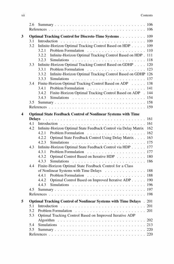
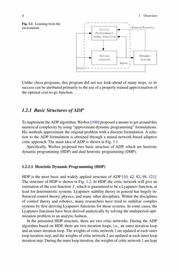
Fig. 1.1 Learning from theenvironment
Unlike chess programs, this program did not use look-ahead of many steps, so itssuccess can be attributed primarily to the use of a properly trained approximation ofthe optimal cost-to-go function.
1.2.1 Basic Structures of ADP
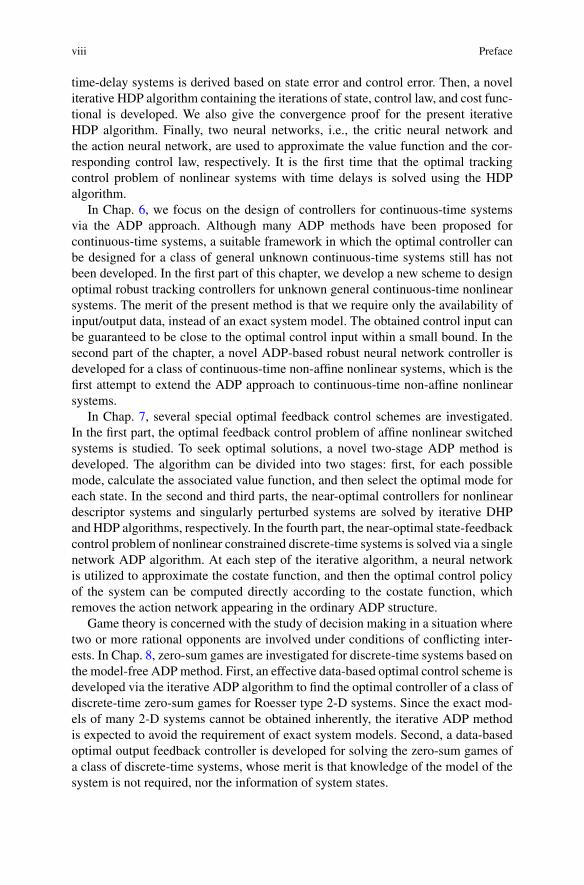
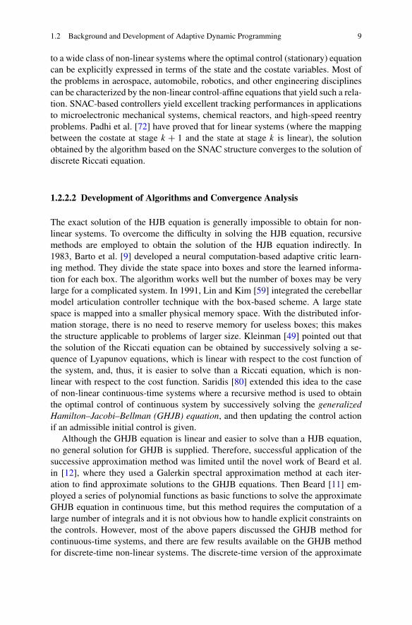
To implement the ADP algorithm, Werbos [100] proposed a means to get around thisnumerical complexity by using “approximate dynamic programming” formulations.His methods approximate the original problem with a discrete formulation. A solu-tion to the ADP formulation is obtained through a neural-network-based adaptivecritic approach. The main idea of ADP is shown in Fig. 1.1.
Specifically, Werbos proposed two basic structure of ADP, which are heuristicdynamic programming (HDP) and dual heuristic programming (DHP).
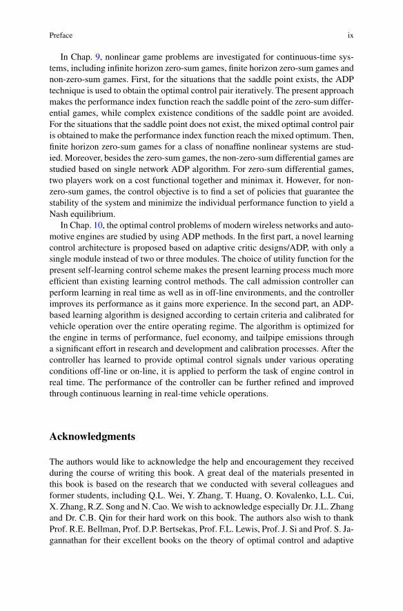
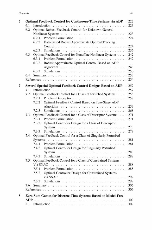
1.2.1.1 Heuristic Dynamic Programming (HDP)
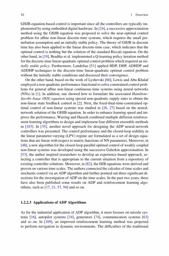
HDP is the most basic and widely applied structure of ADP [10, 42, 82, 98, 121].The structure of HDP is shown in Fig. 1.2. In HDP, the critic network will give anestimation of the cost function J , which is guaranteed to be a Lyapunov function, atleast for deterministic systems. Lyapunov stability theory in general has hugely in-fluenced control theory, physics, and many other disciplines. Within the disciplinesof control theory and robotics, many researchers have tried to stabilize complexsystems by first deriving Lyapunov functions for those systems. In some cases, theLyapunov functions have been derived analytically by solving the multiperiod opti-mization problem in an analytic fashion.
In the presented HDP structure, there are two critic networks. During the ADPalgorithm based on HDP, there are two iteration loops, i.e., an outer iteration loopand an inner iteration loop. The weights of critic network 1 are updated at each outerloop iteration step, and the weights of critic network 2 are updated at each inner loopiteration step. During the inner loop iteration, the weights of critic network 1 are kept
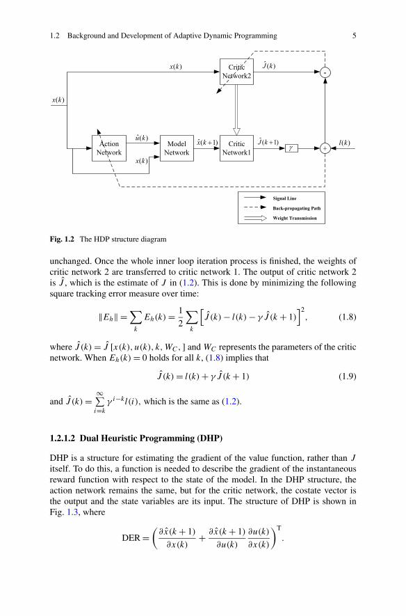
1.2 Background and Development of Adaptive Dynamic Programming 5
Fig. 1.2 The HDP structure diagram
unchanged. Once the whole inner loop iteration process is finished, the weights ofcritic network 2 are transferred to critic network 1. The output of critic network 2is J , which is the estimate of J in (1.2). This is done by minimizing the followingsquare tracking error measure over time:
‖Eh‖ =∑
k
Eh(k)= 1
2
∑
k
[J (k)− l(k)− γ J (k + 1)
]2, (1.8)
where J (k)= J [x(k), u(k), k,WC, ] and WC represents the parameters of the criticnetwork. When Eh(k)= 0 holds for all k, (1.8) implies that
J (k)= l(k)+ γ J (k + 1) (1.9)
and J (k)=∞∑i=k
γ i−kl(i), which is the same as (1.2).
1.2.1.2 Dual Heuristic Programming (DHP)
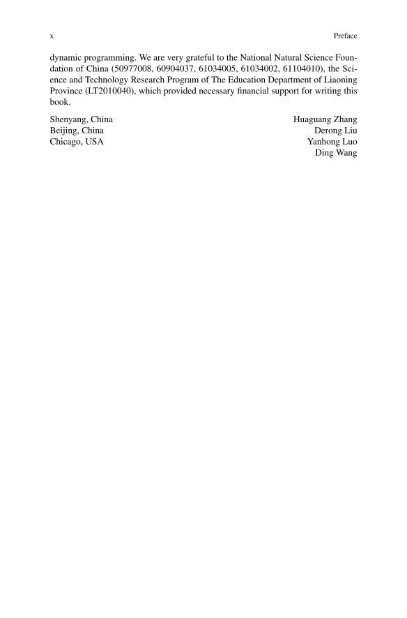
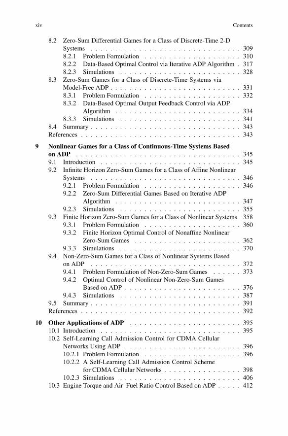
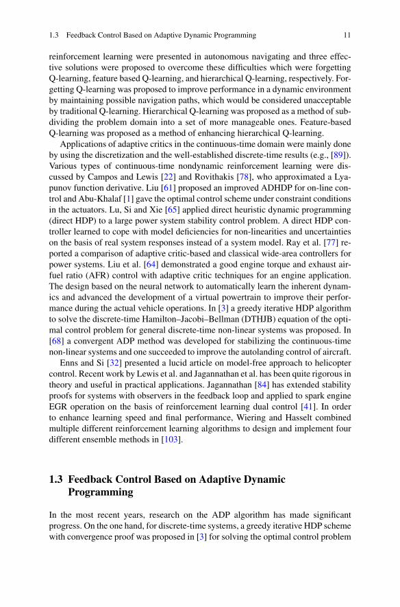
DHP is a structure for estimating the gradient of the value function, rather than J
itself. To do this, a function is needed to describe the gradient of the instantaneousreward function with respect to the state of the model. In the DHP structure, theaction network remains the same, but for the critic network, the costate vector isthe output and the state variables are its input. The structure of DHP is shown inFig. 1.3, where
DER =(∂x(k + 1)
∂x(k)+ ∂x(k + 1)
∂u(k)
∂u(k)
∂x(k)
)T
.
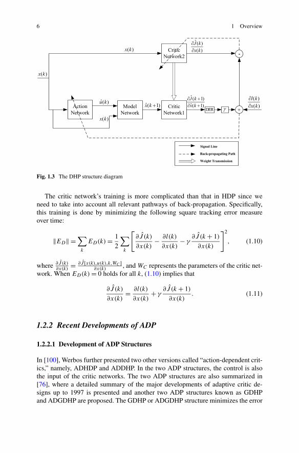
6 1 Overview
Fig. 1.3 The DHP structure diagram
The critic network’s training is more complicated than that in HDP since weneed to take into account all relevant pathways of back-propagation. Specifically,this training is done by minimizing the following square tracking error measureover time:
‖ED‖ =∑
k
ED(k)= 1
2
∑
k
[∂J (k)
∂x(k)− ∂l(k)
∂x(k)− γ
∂J (k + 1)
∂x(k)
]2
, (1.10)
where ∂J (k)∂x(k)
= ∂J [x(k),u(k),k,WC ]∂x(k)
, and WC represents the parameters of the critic net-work. When ED(k)= 0 holds for all k, (1.10) implies that
∂J (k)
∂x(k)= ∂l(k)
∂x(k)+ γ
∂J (k + 1)
∂x(k). (1.11)
1.2.2 Recent Developments of ADP
1.2.2.1 Development of ADP Structures
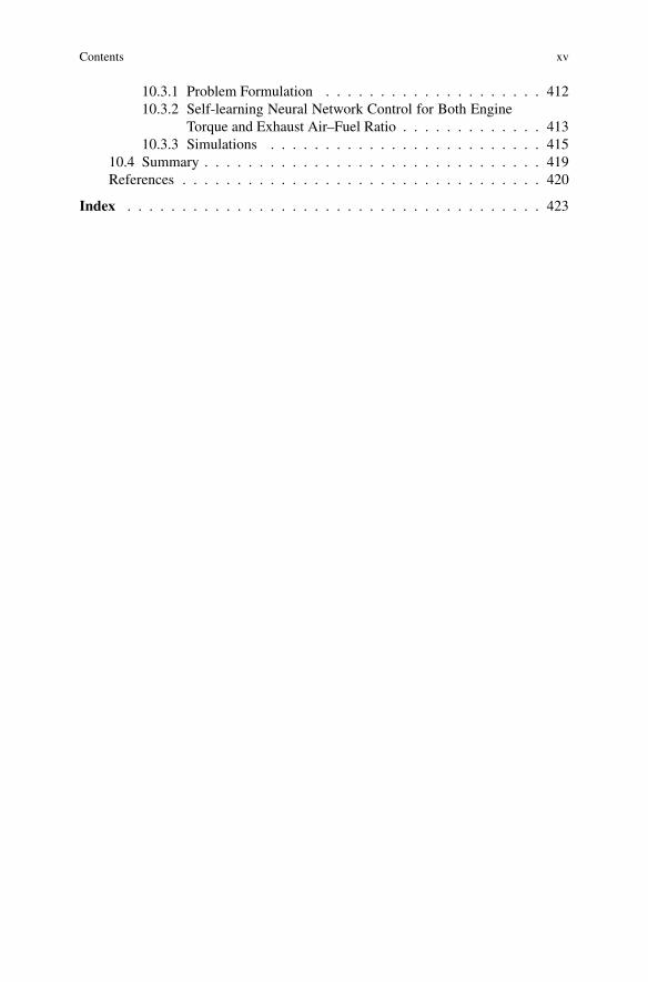
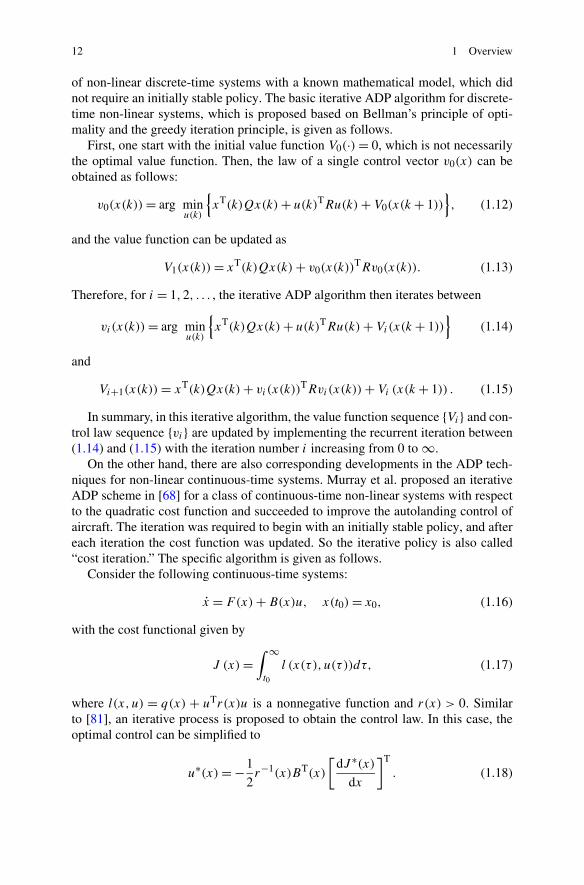
In [100], Werbos further presented two other versions called “action-dependent crit-ics,” namely, ADHDP and ADDHP. In the two ADP structures, the control is alsothe input of the critic networks. The two ADP structures are also summarized in[76], where a detailed summary of the major developments of adaptive critic de-signs up to 1997 is presented and another two ADP structures known as GDHPand ADGDHP are proposed. The GDHP or ADGDHP structure minimizes the error
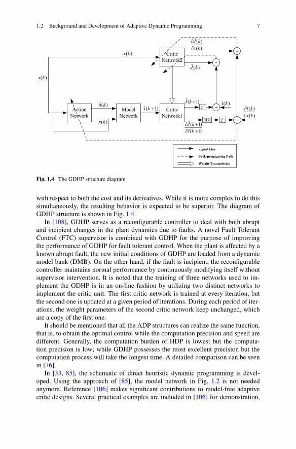
1.2 Background and Development of Adaptive Dynamic Programming 7
Fig. 1.4 The GDHP structure diagram
with respect to both the cost and its derivatives. While it is more complex to do thissimultaneously, the resulting behavior is expected to be superior. The diagram ofGDHP structure is shown in Fig. 1.4.
In [108], GDHP serves as a reconfigurable controller to deal with both abruptand incipient changes in the plant dynamics due to faults. A novel Fault TolerantControl (FTC) supervisor is combined with GDHP for the purpose of improvingthe performance of GDHP for fault tolerant control. When the plant is affected by aknown abrupt fault, the new initial conditions of GDHP are loaded from a dynamicmodel bank (DMB). On the other hand, if the fault is incipient, the reconfigurablecontroller maintains normal performance by continuously modifying itself withoutsupervisor intervention. It is noted that the training of three networks used to im-plement the GDHP is in an on-line fashion by utilizing two distinct networks toimplement the critic unit. The first critic network is trained at every iteration, butthe second one is updated at a given period of iterations. During each period of iter-ations, the weight parameters of the second critic network keep unchanged, whichare a copy of the first one.
It should be mentioned that all the ADP structures can realize the same function,that is, to obtain the optimal control while the computation precision and speed aredifferent. Generally, the computation burden of HDP is lowest but the computa-tion precision is low; while GDHP possesses the most excellent precision but thecomputation process will take the longest time. A detailed comparison can be seenin [76].
In [33, 85], the schematic of direct heuristic dynamic programming is devel-oped. Using the approach of [85], the model network in Fig. 1.2 is not neededanymore. Reference [106] makes significant contributions to model-free adaptivecritic designs. Several practical examples are included in [106] for demonstration,
8 1 Overview
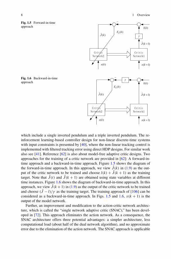
Fig. 1.5 Forward-in-timeapproach
Fig. 1.6 Backward-in-timeapproach
which include a single inverted pendulum and a triple inverted pendulum. The re-inforcement learning-based controller design for non-linear discrete-time systemswith input constraints is presented by [40], where the non-linear tracking control isimplemented with filtered tracking error using direct HDP designs. For similar workalso see [41]. Reference [62] is also about model-free adaptive critic designs. Twoapproaches for the training of a critic network are provided in [62]: A forward-in-time approach and a backward-in-time approach. Figure 1.5 shows the diagram ofthe forward-in-time approach. In this approach, we view J (k) in (1.9) as the out-put of the critic network to be trained and choose l(k) + J (k + 1) as the trainingtarget. Note that J (t) and J (k + 1) are obtained using state variables at differenttime instances. Figure 1.6 shows the diagram of backward-in-time approach. In thisapproach, we view J (k+ 1) in (1.9) as the output of the critic network to be trainedand choose (J − l)/γ as the training target. The training approach of [106] can beconsidered as a backward-in-time approach. In Figs. 1.5 and 1.6, x(k + 1) is theoutput of the model network.
Further, an improvement and modification to the action-critic network architec-ture, which is called the “single network adaptive critic (SNAC),” has been devel-oped in [72]. This approach eliminates the action network. As a consequence, theSNAC architecture offers three potential advantages: a simpler architecture, lesscomputational load (about half of the dual network algorithm), and no approximateerror due to the elimination of the action network. The SNAC approach is applicable
1.2 Background and Development of Adaptive Dynamic Programming 9
to a wide class of non-linear systems where the optimal control (stationary) equationcan be explicitly expressed in terms of the state and the costate variables. Most ofthe problems in aerospace, automobile, robotics, and other engineering disciplinescan be characterized by the non-linear control-affine equations that yield such a rela-tion. SNAC-based controllers yield excellent tracking performances in applicationsto microelectronic mechanical systems, chemical reactors, and high-speed reentryproblems. Padhi et al. [72] have proved that for linear systems (where the mappingbetween the costate at stage k + 1 and the state at stage k is linear), the solutionobtained by the algorithm based on the SNAC structure converges to the solution ofdiscrete Riccati equation.
1.2.2.2 Development of Algorithms and Convergence Analysis
The exact solution of the HJB equation is generally impossible to obtain for non-linear systems. To overcome the difficulty in solving the HJB equation, recursivemethods are employed to obtain the solution of the HJB equation indirectly. In1983, Barto et al. [9] developed a neural computation-based adaptive critic learn-ing method. They divide the state space into boxes and store the learned informa-tion for each box. The algorithm works well but the number of boxes may be verylarge for a complicated system. In 1991, Lin and Kim [59] integrated the cerebellarmodel articulation controller technique with the box-based scheme. A large statespace is mapped into a smaller physical memory space. With the distributed infor-mation storage, there is no need to reserve memory for useless boxes; this makesthe structure applicable to problems of larger size. Kleinman [49] pointed out thatthe solution of the Riccati equation can be obtained by successively solving a se-quence of Lyapunov equations, which is linear with respect to the cost function ofthe system, and, thus, it is easier to solve than a Riccati equation, which is non-linear with respect to the cost function. Saridis [80] extended this idea to the caseof non-linear continuous-time systems where a recursive method is used to obtainthe optimal control of continuous system by successively solving the generalizedHamilton–Jacobi–Bellman (GHJB) equation, and then updating the control actionif an admissible initial control is given.
Although the GHJB equation is linear and easier to solve than a HJB equation,no general solution for GHJB is supplied. Therefore, successful application of thesuccessive approximation method was limited until the novel work of Beard et al.in [12], where they used a Galerkin spectral approximation method at each iter-ation to find approximate solutions to the GHJB equations. Then Beard [11] em-ployed a series of polynomial functions as basic functions to solve the approximateGHJB equation in continuous time, but this method requires the computation of alarge number of integrals and it is not obvious how to handle explicit constraints onthe controls. However, most of the above papers discussed the GHJB method forcontinuous-time systems, and there are few results available on the GHJB methodfor discrete-time non-linear systems. The discrete-time version of the approximate
10 1 Overview
GHJB-equation-based control is important since all the controllers are typically im-plemented by using embedded digital hardware. In [24], a successive approximationmethod using the GHJB equation was proposed to solve the near-optimal controlproblem for affine non-linear discrete-time systems, which requires the small per-turbation assumption and an initially stable policy. The theory of GHJB in discretetime has also been applied to the linear discrete-time case, which indicates that theoptimal control is nothing but the solution of the standard Riccati equation. On theother hand, in [19], Bradtke et al. implemented a Q-learning policy iteration methodfor the discrete-time linear-quadratic optimal control problem which required an ini-tially stable policy. Furthermore, Landelius [51] applied HDP, DHP, ADHDP andADDHP techniques to the discrete-time linear-quadratic optimal control problemwithout the initially stable conditions and discussed their convergence.
On the other hand, based on the work of Lyshevski [66], Lewis and Abu-Khalafemployed a non-quadratic performance functional to solve constrained control prob-lems for general affine non-linear continuous-time systems using neural networks(NNs) in [1]. In addition, one showed how to formulate the associated Hamilton–Jacobi–Isaac (HJI) equation using special non-quadratic supply rates to obtain thenon-linear state feedback control in [2]. Next, the fixed-final-time-constrained op-timal control of non-linear systems was studied in [26, 27] based on the neural-network solution of the GHJB equation. In order to enhance learning speed and im-prove the performance, Wiering and Hasselt combined multiple different reinforce-ment learning algorithms to design and implement four different ensemble methodsin [103]. In [35], another novel approach for designing the ADP neural-networkcontrollers was presented. The control performance and the closed-loop stability inthe linear parameter-varying (LPV) regime are formulated as a set of design equa-tions that are linear with respect to matrix functions of NN parameters. Moreover, in[48], a new algorithm for the closed-loop parallel optimal control of weakly couplednon-linear systems was developed using the successive Galerkin approximation. In[53], the author inspired researchers to develop an experience-based approach, se-lecting a controller that is appropriate to the current situation from a repository ofexisting controller solutions. Moreover, in [82], the HJB equations were derived andproven on various time scales. The authors connected the calculus of time scales andstochastic control via an ADP algorithm and further pointed out three significant di-rections for the investigation of ADP on the time scales. In the past two years, therehave also been published some results on ADP and reinforcement learning algo-rithms, such as [17, 21, 57, 94] and so on.
1.2.2.3 Applications of ADP Algorithms
As for the industrial application of ADP algorithm, it most focuses on missile sys-tems [16], autopilot systems [34], generators [74], communication systems [63]and so on. In [109], an improved reinforcement learning method was proposedto perform navigation in dynamic environments. The difficulties of the traditional
1.3 Feedback Control Based on Adaptive Dynamic Programming 11
reinforcement learning were presented in autonomous navigating and three effec-tive solutions were proposed to overcome these difficulties which were forgettingQ-learning, feature based Q-learning, and hierarchical Q-learning, respectively. For-getting Q-learning was proposed to improve performance in a dynamic environmentby maintaining possible navigation paths, which would be considered unacceptableby traditional Q-learning. Hierarchical Q-learning was proposed as a method of sub-dividing the problem domain into a set of more manageable ones. Feature-basedQ-learning was proposed as a method of enhancing hierarchical Q-learning.
Applications of adaptive critics in the continuous-time domain were mainly doneby using the discretization and the well-established discrete-time results (e.g., [89]).Various types of continuous-time nondynamic reinforcement learning were dis-cussed by Campos and Lewis [22] and Rovithakis [78], who approximated a Lya-punov function derivative. Liu [61] proposed an improved ADHDP for on-line con-trol and Abu-Khalaf [1] gave the optimal control scheme under constraint conditionsin the actuators. Lu, Si and Xie [65] applied direct heuristic dynamic programming(direct HDP) to a large power system stability control problem. A direct HDP con-troller learned to cope with model deficiencies for non-linearities and uncertaintieson the basis of real system responses instead of a system model. Ray et al. [77] re-ported a comparison of adaptive critic-based and classical wide-area controllers forpower systems. Liu et al. [64] demonstrated a good engine torque and exhaust air-fuel ratio (AFR) control with adaptive critic techniques for an engine application.The design based on the neural network to automatically learn the inherent dynam-ics and advanced the development of a virtual powertrain to improve their perfor-mance during the actual vehicle operations. In [3] a greedy iterative HDP algorithmto solve the discrete-time Hamilton–Jacobi–Bellman (DTHJB) equation of the opti-mal control problem for general discrete-time non-linear systems was proposed. In[68] a convergent ADP method was developed for stabilizing the continuous-timenon-linear systems and one succeeded to improve the autolanding control of aircraft.
Enns and Si [32] presented a lucid article on model-free approach to helicoptercontrol. Recent work by Lewis et al. and Jagannathan et al. has been quite rigorous intheory and useful in practical applications. Jagannathan [84] has extended stabilityproofs for systems with observers in the feedback loop and applied to spark engineEGR operation on the basis of reinforcement learning dual control [41]. In orderto enhance learning speed and final performance, Wiering and Hasselt combinedmultiple different reinforcement learning algorithms to design and implement fourdifferent ensemble methods in [103].
1.3 Feedback Control Based on Adaptive DynamicProgramming
In the most recent years, research on the ADP algorithm has made significantprogress. On the one hand, for discrete-time systems, a greedy iterative HDP schemewith convergence proof was proposed in [3] for solving the optimal control problem
12 1 Overview
of non-linear discrete-time systems with a known mathematical model, which didnot require an initially stable policy. The basic iterative ADP algorithm for discrete-time non-linear systems, which is proposed based on Bellman’s principle of opti-mality and the greedy iteration principle, is given as follows.
First, one start with the initial value function V0(·)= 0, which is not necessarilythe optimal value function. Then, the law of a single control vector v0(x) can beobtained as follows:
v0(x(k))= arg minu(k)
{xT(k)Qx(k)+ u(k)TRu(k)+ V0(x(k + 1))
}, (1.12)
and the value function can be updated as
V1(x(k))= xT(k)Qx(k)+ v0(x(k))TRv0(x(k)). (1.13)
Therefore, for i = 1,2, . . . , the iterative ADP algorithm then iterates between
vi(x(k))= arg minu(k)
{xT(k)Qx(k)+ u(k)TRu(k)+ Vi(x(k + 1))
}(1.14)
and
Vi+1(x(k))= xT(k)Qx(k)+ vi(x(k))TRvi(x(k))+ Vi (x(k + 1)) . (1.15)
In summary, in this iterative algorithm, the value function sequence {Vi} and con-trol law sequence {vi} are updated by implementing the recurrent iteration between(1.14) and (1.15) with the iteration number i increasing from 0 to ∞.
On the other hand, there are also corresponding developments in the ADP tech-niques for non-linear continuous-time systems. Murray et al. proposed an iterativeADP scheme in [68] for a class of continuous-time non-linear systems with respectto the quadratic cost function and succeeded to improve the autolanding control ofaircraft. The iteration was required to begin with an initially stable policy, and aftereach iteration the cost function was updated. So the iterative policy is also called“cost iteration.” The specific algorithm is given as follows.
Consider the following continuous-time systems:
x = F(x)+B(x)u, x(t0)= x0, (1.16)
with the cost functional given by
J (x)=∫ ∞
t0
l (x(τ ), u(τ ))dτ, (1.17)
where l(x, u) = q(x) + uTr(x)u is a nonnegative function and r(x) > 0. Similarto [81], an iterative process is proposed to obtain the control law. In this case, theoptimal control can be simplified to
u∗(x)= −1
2r−1(x)BT(x)
[dJ ∗(x)
dx
]T
. (1.18)
1.3 Feedback Control Based on Adaptive Dynamic Programming 13
Starting from any stable Lyapunov function J0 (or alternatively, starting from anarbitrary stable controller u0) and replacing J ∗ by Ji , (1.18) becomes
ui(x)= −1
2r−1(x)BT(x)
[dJi(x)
dx
]T
, (1.19)
where Ji = ∫ +∞t0
l (xi−1, ui−1) dτ is the cost of the trajectory xi−1(t) of plant (1.16)under the input u(t)= ui−1(t). Furthermore, Murray et al. gave a convergence anal-ysis of the iterative ADP scheme and a stability proof of the system. Before that,most of the ADP analysis was based on the Riccati equation for linear systems. In[1], based on the work of Lyshevski [66], an iterative ADP method was used toobtain an approximate solution of the optimal value function of the HJB equationusing NNs. Different from the iterative ADP scheme in [68], the iterative schemein [1] adopted policy iteration, which meant that after each iteration the policy (orcontrol) function was updated. The convergence and stability analysis can also befound in [1].
Moreover, Vrabie et al. [93] proposed a new policy iteration technique to solveon-line the continuous-time LQR problem for a partially model-free system (internaldynamics unknown). They presented an on-line adaptive critic algorithm in whichthe actor performed continuous-time control, whereas the critic’s correction of theactor’s behavior was discrete in time, until best performance was obtained. The criticevaluated the actor’s performance over a period of time and formulated it in a param-eterized form. Policy update was implemented based on the critic’s evaluation on theactor. Convergence of the proposed algorithm was established by proving equiva-lence with an established algorithm [49]. In [35], a novel linear parameter-varying(LPV) approach for designing the ADP neural-network controllers was presented.The control performance and the closed-loop stability of the LPV regime were for-mulated as a set of design equations that were linear with respect to matrix functionsof NN parameters.
It can be seen that most existing results, including the optimal control schemeproposed by Murray et al., require one to implement the algorithm by recurrent iter-ation between the value function and control law, which is not expected in real-timeindustrial applications. Therefore, in [91] and [119], new ADP algorithms were pro-posed to solve the optimal control in an on-line fashion, where the value functionsand control laws were updated simultaneously. The optimal control scheme is re-viewed in the following.
Consider the non-linear system (1.16), and define the infinite-horizon cost func-tional as follows:
J (x,u)=∫ ∞
t
l(x(τ ), u(τ ))dτ, (1.20)
where l(x, u) = xTQx + uTRu is the utility function, and Q and R are symmetricpositive definite matrices with appropriate dimensions.
Define the Hamilton function as
H(x,u,Jx)= J Tx (F (x)+B(x)u)+ xTQx + uTRu, (1.21)
14 1 Overview
where Jx = ∂J (x)/∂x.The optimal value function J ∗(x) is defined as
J ∗(x)= minu∈ψ(�)
∫ ∞
t
l(x(τ ), u(x(τ )))dτ (1.22)
and satisfies
0 = minu∈ψ(�)(H(x,u, J ∗
x )). (1.23)
Therefore, we obtain the optimal control u∗ by solving ∂H(x,u,J ∗x )/∂u= 0, thus:
u∗ = −1
2R−1BT(x)J ∗
x , (1.24)
where J ∗x = ∂J ∗(x)/∂x.
In the following, by employing the critic NN and the action NN, the ADP algo-rithm is implemented to seek for an optimal feedback control law.
First, a neural network is utilized to approximate J (x) as follows:
J (x)=WTc φc(x)+ εc, (1.25)
where Wc is for the unknown ideal constant weights and φc(x) :Rn → RN1 is called
the critic NN activation function vector; N1 is the number of neurons in the hiddenlayer, and εc is the critic NN approximation error.
The derivative of the cost function J (x) with respect to x is
Jx = �φTc Wc +�εc, (1.26)
where �φc � ∂φc(x)/∂x and �εc � ∂εc/∂x.Let Wc be an estimate of Wc; then we have the estimate of J (x) as follows:
J (x)= WTc φc(x). (1.27)
Then the approximate Hamilton function can be derived as follows:
H(x,u, Wa)= WTc �φc(F (x)+B(x)u)+ xTQx + uTRu
= ec. (1.28)
Given any admissible control law u, it is desired to select Wc to minimize thesquared residual error Ec(Wc) as follows:
Ec(Wc)= 1
2eTc ec. (1.29)
The weight update law for the critic NN is presented based on a gradient descentalgorithm, which is given by
˙Wc = −αcσc(φ
Tc Wc + xTQx + uTRu), (1.30)
1.3 Feedback Control Based on Adaptive Dynamic Programming 15
where αc > 0 is the adaptive gain of the critic NN, σc = σ/(σTσ + 1),σ = �φc(F (x)+B(x)u).
On the other hand, the feedback control u is approximated by the action NN as
u=WTa φa(x)+ εa, (1.31)
where Wa is the matrix of unknown ideal constant weights and φa(x) : Rn → RN2
is called the action NN activation function vector, N2 is the number of neurons inthe hidden layer, and εa is the action NN approximation error.
Let Wa be an estimate of Wa ; then the actual output can be expressed as
u= WTa φa(x). (1.32)
The feedback error signal used for tuning action NN is defined as
ea = WTa φa + 1
2R−1Cu�φT
c Wc. (1.33)
The objective function to be minimized by the action NN is defined as
Ea(Wa)= 1
2eTa ea. (1.34)
The weight update law for the action NN is designed based on the gradient de-scent algorithm, which is given by
˙Wa = −αaφa
(WT
a φa + 1
2R−1Cu�φT
c Wc
)T
, (1.35)
where αa > 0 is the adaptive gain of the action NN.After the presentation of the weight update rule, a stability analysis of the closed-
loop system can be performed based on the Lyapunov approach to guarantee theboundness of the weight parameters [119].
It should be mentioned that most of the above results require the models of thecontrolled plants to be known or at least partially known. However, in practicalapplications, most models cannot be obtained. Therefore, it is necessary to recon-struct the non-linear systems with function approximators. Recurrent neural net-works (RNNs) are one kind of NN models, which are widely used in the dynamicalanalysis of non-linear systems, such as [115, 118, 123]. In this book, we will presentthe specific method for modeling the non-linear systems with RNN. Based on theRNN model, the ADP algorithm can be properly introduced to deal with the optimalcontrol problems of unknown non-linear systems.
Meanwhile, saturation, dead-zones, backlash, and hysteresis are the most com-mon actuator non-linearities in practical control system applications. Saturationnon-linearity is unavoidable in most actuators. Due to the nonanalytic nature ofthe actuator’s non-linear dynamics and the fact that the exact actuator’s non-linearfunctions are unknown, such systems present a challenge to control engineers. As
16 1 Overview
far as we know, most of the existing results of dealing with the control of systemswith saturating actuators do not refer to the optimal control laws. Therefore, thisproblem is worthy of study in the framework of the HJB equation. To the best ofour knowledge, though ADP algorithms have made large progress in the optimalcontrol field, it is still an open problem how to solve the optimal control problemfor discrete-time systems with control constraints based on ADP algorithms. If theactuator has saturating characteristic, how do we find a constrained optimal control?In this book, we shall give positive answers to these questions.
Moreover, traditional optimal control approaches are mostly implemented in aninfinite time horizon. However, most real-world systems need to be effectively con-trolled within a finite time horizon (finite horizon for brief), such as stabilized onesor ones tracked to a desired trajectory in a finite duration of time. The design offinite-horizon optimal controllers faces a huge obstacle in comparison to the infinite-horizon one. An infinite-horizon optimal controller generally obtains an asymptoticresult for the controlled systems [73]. That is, the system will not be stabilized ortracked until the time reaches infinity, while for finite-horizon optimal control prob-lems, the system must be stabilized or tracked to a desired trajectory in a finite dura-tion of time [20, 70, 90, 107, 111]. Furthermore, in the case of discrete-time systems,a determination of the number of optimal control steps is necessary for finite-horizonoptimal control problems, while for the infinite-horizon optimal control problems,the number of optimal control steps is infinite in general. The finite-horizon controlproblem has been addressed by many researchers [18, 28, 37, 110, 116]. But mostof the existing methods consider only stability problems of systems under finite-horizon controllers [18, 37, 110, 116]. Due to the lack of methodology and the factthat the number of control steps is difficult to determine, the optimal controller de-sign of finite-horizon problems still presents a major challenge to control engineers.
In this book, we will develop a new ADP scheme for finite-horizon optimal con-trol problems. We will study the optimal control problems with an ε-error boundusing ADP algorithms. First, the HJB equation for finite-horizon optimal control ofdiscrete-time systems is derived. In order to solve this HJB equation, a new iterativeADP algorithm is developed with convergence and optimality proofs. Second, thedifficulties of obtaining the optimal solution using the iterative ADP algorithm ispresented and then the ε-optimal control algorithm is derived based on the iterativeADP algorithms. Next, it will be shown that the ε-optimal control algorithm can ob-tain suboptimal control solutions within a fixed finite number of control steps thatmake the value function converge to its optimal value with an ε-error.
It should be mentioned that all the above results based on ADP do not refer to thesystems with time delays. Actually, time delay often occurs in the transmission be-tween different parts of systems. Transportation systems, communication systems,chemical processing systems, metallurgical processing systems and power systemsare examples of time-delay systems. Therefore, the investigation of time-delay sys-tems is significant. In recent years, much researches has been performed on decen-tralized control, synchronization control and stability analysis [112, 114, 117, 122].However, the optimal control problem is often encountered in industrial produc-tion. In general, optimal control for time-delay systems is an infinite-dimensional
1.4 Non-linear Games Based on Adaptive Dynamic Programming 17
control problem [67], which is very difficult to solve. The analysis of systems withtime delays is much more difficult than that of systems without delays, and thereis no method strictly facing this problem for non-linear time-delay systems. So inthis book, optimal state feedback control problems of non-linear systems with timedelays will also be discussed.
1.4 Non-linear Games Based on Adaptive DynamicProgramming
All of the above results discuss the situation that there is only one controller to bedesigned. However, as is known, a large class of real systems are controlled by morethan one controller or decision maker with each using an individual strategy. Thesecontrollers often operate in a group with a general quadratic cost functional as agame [45]. Zero-sum differential game theory has been widely applied to decisionmaking problems [23, 25, 38, 44, 52, 55], stimulated by a vast number of applica-tions, including those in economy, management, communication networks, powernetworks, and in the design of complex engineering systems.
In recent years, based on the work of [51], approximate dynamic programming(ADP) techniques have further been extended to the zero-sum games of linear andnon-linear systems. In [4, 5], HDP and DHP structures were used to solve thediscrete-time linear-quadratic zero-sum games appearing in the H∞ optimal con-trol problem. The optimal strategies for discrete-time quadratic zero-sum gamesrelated to the H∞ optimal control problem were solved forward in time. The ideais to solve for an action-dependent cost function Q(x,u,w) of the zero-sum games,instead of solving for the state-dependent cost function J (x) which satisfies a cor-responding game algebraic Riccati equation (GARE). Using the Kronecker method,two action networks and one critic network were adaptively tuned forward in timeusing adaptive critic methods without the information of a model of the system.The algorithm was proved to converge to the Nash equilibrium of the correspondingzero-sum games. The performance comparisons were carried out on an F-16 autopi-lot. Then, in [6] these results were extended to a model-free environment for thecontrol of a power generator system. In the paper, the on-line model-free adaptivecritic schemes based on ADP were presented by the authors to solve optimal con-trol problems in both discrete-time and continuous-time domains for linear systemswith unknown dynamics. In the discrete-time case, the solution process leads tosolving the underlying game GARE of the corresponding optimal control problemor zero-sum games. In the continuous-time domain, their ADP scheme solves theunderlying algebraic Riccati equation (ARE) of the optimal control problem. Theyshow that their continuous-time ADP scheme is nothing but a quasi-Newton methodto solve the ARE. Either in continuous-time domain or discrete-time domain, theadaptive critic algorithms are easy to initialize considering that initial policies arenot required to be stabilizing.
In the following, we present some basic knowledge regarding non-linear zero-sum differential games first [120].
18 1 Overview
Consider the following two-person zero-sum differential games. The state tra-jectory of the game is described by the following continuous-time affine non-linearfunction:
x = f (x,u,w)= a(x)+ b(x)u+ c(x)w, (1.36)
where x ∈ Rn, u ∈ R
k , w ∈Rm and the initial condition x(0)= x0 is given.
The two control variables u and w are functions chosen on [0,∞) by player I andplayer II from some control sets U [0,∞) and W [0,∞), respectively, subject to theconstraints u ∈ U(t), and w ∈ W(t) for t ∈ [0,∞), for given convex and compactsets U(t) ⊂ R
k , W(t) ⊂ Rm. The cost functional is a generalized quadratic form
given by
J (x(0), u,w)=∫ ∞
0(xTAx + uTBu+wTCw
+ 2uTDw + 2xTEu+ 2xTFw)dt, (1.37)
where matrices A,B,C,D,E,F have suitable dimension and A≥ 0, B > 0, C < 0.So we see, for ∀t ∈ [0,∞), that the cost functional J (x(t), u,w) (denoted byJ (x) for brevity in the sequel) is convex in u and concave in w. l(x, u,w) =xTAx + uTBu + wTCw + 2uTDw + 2xTEu + 2xTFw is the general quadraticutility function. For the above zero-sum differential games, there are two controllersor players where player I tries to minimize the cost functional J (x), while player IIattempts to maximize it. According to the situation of the two players, the followingdefinitions are presented first.
Let
J (x) := infu∈U [t,∞)
supw∈W [t,∞)
J (x,u,w) (1.38)
be the upper value function and
J (x) := supw∈W [t,∞)
infu∈U [t,∞)
J (x,u,w) (1.39)
be the lower value function with the obvious inequality J (x) ≥ J (x). Define theoptimal control pairs be (u,w) and (u,w) for upper and lower value function, re-spectively. Then, we have
J (x)= J (x,u,w) (1.40)
and
J (x)= J (x,u,w). (1.41)
If both J (x) and J (x) exist and
J (x)= J (x)= J ∗(x), (1.42)
we say that the optimal value function of the zero-sum differential games or the sad-dle point exists and the corresponding optimal control pair is denoted by (u∗,w∗).
1.5 Summary 19
As far as we know, traditional approaches in dealing with zero-sum differentialgames are to find the optimal solution or the saddle point of the games. So manyresults are developed to discuss the existence conditions of the differential zero-sumgames [36, 113].
In the real world, however, the existence conditions of the saddle point for zero-sum differential games are so difficult to satisfy that many applications of the zero-sum differential games are limited to linear systems [31, 43, 47]. On the other hand,for many zero-sum differential games, especially in the non-linear case, the opti-mal solution of the game (or saddle point) does not exist inherently. Therefore, it isnecessary to study the optimal control approach for the zero-sum differential gameswhere the saddle point is invalid. The earlier optimal control scheme is to adopt themixed trajectory method [14, 71], in which one player selects an optimal probabilitydistribution over his control set and the other player selects an optimal probabilitydistribution over his own control set, and then the expected solution of the game canbe obtained in the sense of probability. The expected solution of the game is calleda mixed optimal solution and the corresponding value function is the mixed optimalvalue function. The main difficulty of the mixed trajectory for the zero-sum differ-ential games is that the optimal probability distribution is too hard, if not impossible,to obtain for the whole real space. Furthermore, the mixed optimal solution is hardlyreached once the control schemes are determined. In most cases (i.e. in engineer-ing cases), however, the optimal solution or mixed optimal solution of the zero-sumdifferential games has to be achieved by a determined optimal or mixed optimalcontrol scheme. In order to overcome these difficulties, a new iterative approach isdeveloped in this book to solve zero-sum differential games for a non-linear system.
1.5 Summary
In this chapter, we briefly introduced the variations on the structure of ADP schemesand stated the development of the iterative ADP algorithms, and, finally, we recallthe industrial application of ADP schemes. Due to the focus of the book, we do notlist all the methods developed in ADP. Our attention is to give an introduction to thedevelopment of theory so as to provide a rough description of ADP for a new-comerin research in this area.
References
1. Abu-Khalaf M, Lewis FL (2005) Nearly optimal control laws for nonlinear systems withsaturating actuators using a neural network HJB approach. Automatica 41(5):779–791
2. Abu-Khalaf M, Lewis FL, Huang J (2006) Policy iterations on the Hamilton–Jacobi–Isaacs equation for state feedback control with input saturation. IEEE Trans Autom Control51(12):1989–1995
3. Al-Tamimi A, Lewis FL (2007) Discrete-time nonlinear HJB solution using approximate dy-namic programming: convergence proof. In: Proceedings of IEEE international symposiumon approximate dynamic programming and reinforcement learning, Honolulu, HI, pp 38–43
20 1 Overview
4. Al-Tamimi A, Abu-Khalaf M, Lewis FL (2007) Adaptive critic designs for discrete-timezero-sum games with application to H∞ control. IEEE Trans Syst Man Cybern, Part B,Cybern 37(1):240–247
5. Al-Tamimi A, Lewis FL, Abu-Khalaf M (2007) Model-free Q-learning designs for lineardiscrete-time zero-sum games with application to H-infinity control. Automatica 43(3):473–481
6. Al-Tamimi A, Lewis FL, Wang Y (2007) Model-free H-infinity load-frequency controllerdesign for power systems. In: Proceedings of IEEE international symposium on intelligentcontrol, pp 118–125
7. Al-Tamimi A, Lewis FL, Abu-Khalaf M (2008) Discrete-time nonlinear HJB solution usingapproximate dynamic programming: convergence proof. IEEE Trans Syst Man Cybern, PartB, Cybern 38(4):943–949
8. Bardi M, Capuzzo-Dolcetta I (1997) Optimal control and viscosity solutions of Hamilton–Jacobi–Bellman equations. Birkhauser, Boston
9. Barto AG, Sutton RS, Anderson CW (1983) Neuronlike adaptive elements that can solvedifficult learning control problems. IEEE Trans Syst Man Cybern 13(5):835–846
10. Beard RW (1995) Improving the closed-loop performance of nonlinear systems. PhD disser-tation, Rensselaer Polytech Institute, Troy, NY
11. Beard RW, Saridis GN (1998) Approximate solutions to the timeinvariant Hamilton–Jacobi–Bellman equation. J Optim Theory Appl 96(3):589–626
12. Beard RW, Saridis GN, Wen JT (1997) Galerkin approximations of the generalizedHamilton–Jacobi–Bellman equation. Automatica 33(12):2159–2177
13. Bellman RE (1957) Dynamic programming. Princeton University Press, Princeton14. Bertsekas DP (2003) Convex analysis and optimization. Athena Scientific, Belmont15. Bertsekas DP, Tsitsiklis JN (1996) Neuro-dynamic programming. Athena Scientific, Bel-
mont16. Bertsekas DP, Homer ML, Logan DA, Patek SD, Sandell NR (2000) Missile defense and
interceptor allocation by neuro-dynamic programming. IEEE Trans Syst Man Cybern, PartA, Syst Hum 30(1):42–51
17. Bhasin S, Sharma N, Patre P, Dixon WE (2011) Asymptotic tracking by a reinforcementlearning-based adaptive critic controller. J Control Theory Appl 9(3):400–409
18. Blackmore L, Rajamanoharan S, Williams BC (2008) Active estimation for jump Markovlinear systems. IEEE Trans Autom Control 53(10):2223–2236
19. Bradtke SJ, Ydestie BE, Barto AG (1994) Adaptive linear quadratic control using policy it-eration. In: Proceedings of the American control conference, Baltimore, Maryland, pp 3475–3476
20. Bryson AE, Ho YC (1975) Applied optimal control: optimization, estimation, and control.Hemisphere–Wiley, New York
21. Busoniu L, Babuska R, Schutter BD, Ernst D (2010) Reinforcement learning and dynamicprogramming using function approximators. CRC Press, Boca Raton
22. Campos J, Lewis FL (1999) Adaptive critic neural network for feedforward compensation.In: Proceedings of American control conference, San Diego, CA, pp 2813–2818
23. Chang HS, Marcus SI (2003) Two-person zero-sum Markov games: receding horizon ap-proach. IEEE Trans Autom Control 48(11):1951–1961
24. Chen Z, Jagannathan S (2008) Generalized Hamilton–Jacobi–Bellman formulation-basedneural network control of affine nonlinear discrete-time systems. IEEE Trans Neural Netw19(1):90–106
25. Chen BS, Tseng CS, Uang HJ (2002) Fuzzy differential games for nonlinear stochastic sys-tems: suboptimal approach. IEEE Trans Fuzzy Syst 10(2):222–233
26. Cheng T, Lewis FL, Abu-Khalaf M (2007) Fixed-final-time-constrained optimal con-trol of nonlinear systems using neural network HJB approach. IEEE Trans Neural Netw18(6):1725–1736
27. Cheng T, Lewis FL, Abu-Khalaf M (2007) A neural network solution for fixed-final timeoptimal control of nonlinear systems. Automatica 43(3):482–490
References 21
28. Costa OLV, Tuesta EF (2003) Finite horizon quadratic optimal control and a separation prin-ciple for Markovian jump linear systems. IEEE Trans Autom Control 48:1836–1842
29. Dalton J, Balakrishnan SN (1996) A neighboring optimal adaptive critic for missile guidance.Math Comput Model 23:175–188
30. Dreyfus SE, Law AM (1977) The art and theory of dynamic programming. Academic Press,New York
31. Engwerda J (2008) Uniqueness conditions for the affine open-loop linear quadratic differen-tial game. Automatica 44(2):504–511
32. Enns R, Si J (2002) Apache helicopter stabilization using neural dynamic programming. JGuid Control Dyn 25(1):19–25
33. Enns R, Si J (2003) Helicopter trimming and tracking control using direct neural dynamicprogramming. IEEE Trans Neural Netw 14(4):929–939
34. Ferrari S, Stengel RF (2004) Online adaptive critic flight control. J Guid Control Dyn27(5):777–786
35. Ferrari S, Steck JE, Chandramohan R (2008) Adaptive feedback control by constrained ap-proximate dynamic programming. IEEE Trans Syst Man Cybern, Part B, Cybern 38(4):982–987
36. Goebel R (2002) Convexity in zero-sum differential games. In: Proceedings of the 41th IEEEconference on decision and control, Las Vegas, Nevada, pp 3964–3969
37. Goulart PJ, Kerrigan EC, Alamo T (2009) Control of constrained discrete-time systems withbounded L2 gain. IEEE Trans Autom Control 54(5):1105–1111
38. Gu D (2008) A differential game approach to formation control. IEEE Trans Control SystTechnol 16(1):85–93
39. Hanselmann T, Noakes L, Zaknich A (2007) Continuous-time adaptive critics. IEEE TransNeural Netw 18(3):631–647
40. He P, Jagannathan S (2005) Reinforcement learning-based output feedback control of nonlin-ear systems with input constraints. IEEE Trans Syst Man Cybern, Part B, Cybern 35(1):150–154
41. He P, Jagannathan S (2007) Reinforcement learning neural-network-based controller fornonlinear discrete-time systems with input constraints. IEEE Trans Syst Man Cybern, PartB, Cybern 37(2):425–436
42. Hou ZG, Wu CP (2005) A dynamic programming neural network for large-scale optimizationproblems. Acta Autom Sin 25(1):46–51
43. Hua X, Mizukami K (1994) Linear-quadratic zero-sum differential games for generalizedstate space systems. IEEE Trans Autom Control 39(1):143–147
44. Hwnag KS, Chiou JY, Chen TY (2004) Reinforcement learning in zero-sum Markov gamesfor robot soccer systems. In: Proceedings of the 2004 IEEE international conference on net-working, sensing and control, Taipei, Taiwan, pp 1110–1114
45. Jamshidi M (1982) Large-scale systems-modeling and control. North-Holland, Amsterdam46. Javaherian H, Liu D, Zhang Y, Kovalenko O (2004) Adaptive critic learning techniques for
automotive engine control. In: Proceedings of American control conference, Boston, MA, pp4066–4071
47. Jimenez M, Poznyak A (2006) Robust and adaptive strategies with pre-identification viasliding mode technique in LQ differential games. In: Proceedings of American control con-ference Minneapolis, Minnesota, USA, pp 14–16
48. Kim YJ, Lim MT (2008) Parallel optimal control for weakly coupled nonlinear systems usingsuccessive Galerkin approximation. IEEE Trans Autom Control 53(6):1542–1547
49. Kleinman D (1968) On an iterative technique for Riccati equation computations. IEEE TransAutom Control 13(1):114–115
50. Kulkarni NV, KrishnaKumar K (2003) Intelligent engine control using an adaptive critic.IEEE Trans Control Syst Technol 11:164–173
51. Landelius T (1997) Reinforcement learning and distributed local model synthesis. PhD dis-sertation, Linkoping University, Sweden
22 1 Overview
52. Laraki R, Solan E (2005) The value of zero-sum stopping games in continuous time. SIAMJ Control Optim 43(5):1913–1922
53. Lendaris GG (2008) Higher level application of ADP: a nextphase for the control field. IEEETrans Syst Man Cybern, Part B, Cybern 38(4):901–912
54. Lendaris GG, Paintz C (1997) Training strategies for critic and action neural networks in dualheuristic programming method. In: Proceedings of the 1997 IEEE international conferenceon neural networks, Houston, TX, pp 712–717
55. Leslie DS, Collins EJ (2005) Individual Q-learning in normal form games. SIAM J ControlOptim 44(2):495–514
56. Lewis FL (1992) Applied optimal control and estimation. Texas instruments. Prentice Hall,Englewood Cliffs
57. Lewis FL, Liu D (2012) Reinforcement learning and approximate dynamic programming forfeedback control. IEEE press series on computational intelligence. Wiley, New York
58. Lewis FL, Syrmos VL (1992) Optimal control. Wiley, New York59. Lin CS, Kim H (1991) CMAC-based adaptive critic self-learning control. IEEE Trans Neural
Netw 2(5):530–53360. Liu X, Balakrishnan SN (2000) Convergence analysis of adaptive critic based optimal con-
trol. In: Proceedings of American control conference, Chicago, Illinois, pp 1929–193361. Liu D, Zhang HG (2005) A neural dynamic programming approach for learning control of
failure avoidance problems. Int J Intell Control Syst 10(1):21–3262. Liu D, Xiong X, Zhang Y (2001) Action-dependent adaptive critic designs. In: Proceeding
of international joint conference on neural networks, Washington, DC, pp 990–99563. Liu D, Zhang Y, Zhang HG (2005) A self-learning call admission control scheme for CDMA
cellular networks. IEEE Trans Neural Netw 16(5):1219–122864. Liu D, Javaherian H, Kovalenko O, Huang T (2008) Adaptive critic learning techniques
for engine torque and air–fuel ratio control. IEEE Trans Syst Man Cybern, Part B, Cybern38(4):988–993
65. Lu C, Si J, Xie X (2008) Direct heuristic dynamic programming for damping oscillations ina large power system. IEEE Trans Syst Man Cybern, Part B, Cybern 38(4):1008–1013
66. Lyshevski SE (2002) Optimization of dynamic systems using novel performance functionals.In: Proceedings of 41st IEEE conference on decision and control, Las Vegas, Nevada, pp753–758
67. Malek-Zavarei M, Jashmidi M (1987) Time-delay systems: analysis, optimization and appli-cations North-Holland, Amsterdam, pp 80–96
68. Murray JJ, Cox CJ, Lendaris GG, Saeks R (2002) Adaptive dynamic programming. IEEETrans Syst Man Cybern, Part C, Appl Rev 32(2):140–153
69. Murray JJ, Cox CJ, Saeks R (2003) The adaptive dynamic programming theorem. In: Liu D,Antsaklis PJ (eds) Stability and control of dynamical systems with applications. Birkhäser,Boston, pp 379–394
70. Necoara I, Kerrigan EC, Schutter BD, Boom T (2007) Finite-horizon min–max control ofmax-plus-linear systems. IEEE Trans Autom Control 52(6):1088–1093
71. Owen G (1982) Game theory. Academic Press, New York72. Padhi R, Unnikrishnan N, Wang X, Balakrishnan SN (2006) A single network adaptive critic
(SNAC) architecture for optimal control synthesis for a class of nonlinear systems. NeuralNetw 19(10):1648–1660
73. Parisini T, Zoppoli R (1998) Neural approximations for infinite-horizon optimal control ofnonlinear stochastic systems. IEEE Trans Neural Netw 9(6):1388–1408
74. Park JW, Harley RG, Venayagamoorthy GK (2003) Adaptive-critic-based optimal neurocon-trol for synchronous generators in a power system using MLP/RBF neural networks. IEEETrans Ind Appl 39:1529–1540
75. Powell WB (2011) Approximate dynamic programming: solving the curses of dimensional-ity, 2nd edn. Wiley, Princeton
76. Prokhorov DV, Wunsch DC (1997) Adaptive critic designs. IEEE Trans Neural Netw8(5):997–1007
References 23
77. Ray S, Venayagamoorthy GK, Chaudhuri B, Majumder R (2008) Comparison of adaptivecritic-based and classical wide-area controllers for power systems. IEEE Trans Syst ManCybern, Part B, Cybern 38(4):1002–1007
78. Rovithakis GA (2001) Stable adaptive neuro-control design via Lyapunov function derivativeestimation. Automatica 37(8):1213–1221
79. Saeks RE, Cox CJ, Mathia K, Maren AJ (1997) Asymptotic dynamic programming: prelim-inary concepts and results. In: Proceedings of the 1997 IEEE international conference onneural networks, Houston, TX, pp 2273–2278
80. Saridis GN, Lee CS (1979) An approximation theory of optimal control for trainable manip-ulators. IEEE Trans Syst Man Cybern 9(3):152–159
81. Saridis GN, Wang FY (1994) Suboptimal control of nonlinear stochastic systems. ControlTheory Adv Technol 10(4):847–871
82. Seiffertt J, Sanyal S, Wunsch DC (2008) Hamilton–Jacobi–Bellman equations and approx-imate dynamic programming on time scales. IEEE Trans Syst Man Cybern, Part B, Cybern38(4):918–923
83. Shervais S, Shannon TT, Lendaris GG (2003) Intelligent supply chain management usingadaptive critic learning. IEEE Trans Syst Man Cybern, Part A, Syst Hum 33(2):235–244
84. Shih P, Kaul B, Jagannathan S, Drallmeier J (2007) Near optimal output-feedback controlof nonlinear discrete-time systems in nonstrict feedback form with application to engines.In: Proceedings of international joint conference on neural networks, Orlando, Florida, pp396–401
85. Si J, Wang YT (2001) On-line learning control by association and reinforcement. IEEE TransNeural Netw 12(2):264–276
86. Si J, Barto A, Powell W, Wunsch D (2004) Handbook of learning dynamic programming.Wiley, New Jersey
87. Sutton RS, Barto AG (1998) Reinforcement learning: an introduction. MIT Press, Cam-bridge
88. Tesauro GJ (2000) Practical issues in temporal difference learning. Mach Learn 8:257–27789. Tsitsiklis JN (1995) Efficient algorithms for globally optimal trajectories. IEEE Trans Autom
Control 40(9):1528–153890. Uchida K, Fujita M (1992) Finite horizon H∞ control problems with terminal penalties.
IEEE Trans Autom Control 37(11):1762–176791. Vamvoudakis KG, Lewis FL (2010) Online actor-critic algorithm to solve the continuous-
time infinite horizon optimal control problem. Automatica 46:878–88892. Venayagamoorthy GK, Harley RG, Wunsch DG (2002) Comparison of heuristic dynamic
programming and dual heuristic programming adaptive critics for neurocontrol of a turbo-generator. IEEE Trans Neural Netw 13:764–773
93. Vrabie D, Abu-Khalaf M, Lewis FL, Wang Y (2007) Continuous-time ADP for linear sys-tems with partially unknown dynamics. In: Proceedings of the 2007 IEEE symposium onapproximate dynamic programming and reinforcement learning, Honolulu, USA, pp 247–253
94. Vrabie D, Vamvoudakis KG, Lewis FL (2012) Optimal adaptive control and differentialgames by reinforcement learning principles. IET Press, London
95. Watkins C (1989) Learning from delayed rewards. PhD dissertation, Cambridge University,Cambridge, England
96. Werbos PJ (1977) Advanced forecasting methods for global crisis warning and models ofintelligence. Gen Syst Yearbook 22:25–38
97. Werbos PJ (1987) Building and understanding adaptive systems: a statistical/numerical ap-proach to factory automation and brain research. IEEE Trans Syst Man Cybern 17(1):7–20
98. Werbos PJ (1990) Consistency of HDP applied to a simple reinforcement learning problem.Neural Netw 3(2):179–189
99. Werbos PJ (1990) A menu of designs for reinforcement learning over time. In: Miller WT,Sutton RS, Werbos PJ (eds) Neural networks for control. MIT Press, Cambridge, pp 67–95
24 1 Overview
100. Werbos PJ (1992) Approximate dynamic programming for real-time control and neural mod-eling. In: White DA, Sofge DA (eds) Handbook of intelligent control: neural, fuzzy andadaptive approaches. Van Nostrand, New York, chap 13
101. Werbos PJ (2007) Using ADP to understand and replicate brain intelligence: the next leveldesign. In: Proceedings of IEEE symposium on approximate dynamic programming and re-inforcement learning, Honolulu, HI, pp 209–216
102. Widrow B, Gupta N, Maitra S (1973) Punish/reward: learning with a critic in adaptive thresh-old systems. IEEE Trans Syst Man Cybern 3(5):455–465
103. Wiering MA, Hasselt HV (2008) Ensemble algorithms in reinforcement learning. IEEE TransSyst Man Cybern, Part B, Cybern 38(4):930–936
104. Yadav V, Padhi R, Balakrishnan SN (2007) Robust/optimal temperature profile control of ahigh-speed aerospace vehicle using neural networks. IEEE Trans Neural Netw 18(4):1115–1128
105. Yang Q, Jagannathan S (2007) Online reinforcement learning neural network controller de-sign for nanomanipulation. In: Proceedings of IEEE symposium on approximate dynamicprogramming and reinforcement learning, Honolulu, HI, pp 225–232
106. Yang L, Enns R, Wang YT, Si J (2003) Direct neural dynamic programming. In: Liu D,Antsaklis PJ (eds) Stability and control of dynamical systems with applications. Birkhauser,Boston
107. Yang F, Wang Z, Feng G, Liu X (2009) Robust filtering with randomly varying sensor delay:the finite-horizon case. IEEE Trans Circuits Syst I, Regul Pap 56(3):664–672
108. Yen GG, DeLima PG (2005) Improving the performance of globalized dual heuristic pro-gramming for fault tolerant control through an online learning supervisor. IEEE Trans AutomSci Eng 2(2):121–131
109. Yen GG, Hickey TW (2004) Reinforcement learning algorithms for robotic navigation indynamic environments. ISA Trans 43:217–230
110. Zadorojniy A, Shwartz A (2006) Robustness of policies in constrained Markov decision pro-cesses. IEEE Trans Autom Control 51(4):635–638
111. Zattoni E (2008) Structural invariant subspaces of singular Hamiltonian systems and non-recursive solutions of finite-horizon optimal control problems. IEEE Trans Autom Control53(5):1279–1284
112. Zhang HG, Wang ZS (2007) Global asymptotic stability of delayed cellular neural networks.IEEE Trans Neural Netw 18(3):947–950
113. Zhang P, Deng H, Xi J (2005) On the value of two-person zero-sum linear quadratic differ-ential games. In: Proceedings of the 44th IEEE conference on decision and control, and theEuropean control conference. Seville, Spain, pp 12–15
114. Zhang HG, Lun SX, Liu D (2007) Fuzzy H(infinity) filter design for a class of nonlineardiscrete-time systems with multiple time delays. IEEE Trans Fuzzy Syst 15(3):453–469
115. Zhang HG, Wang ZS, Liu D (2007) Robust exponential stability of recurrent neural networkswith multiple time-varying delays. IEEE Trans Circuits Syst II, Express Briefs 54(8):730–734
116. Zhang HS, Xie L, Duan G (2007) H∞ control of discrete-time systems with multiple inputdelays. IEEE Trans Autom Control 52(2):271–283
117. Zhang HG, Yang DD, Chai TY (2007) Guaranteed cost networked control for T-S fuzzysystems with time delays. IEEE Trans Syst Man Cybern, Part C, Appl Rev 37(2):160–172
118. Zhang HG, Ma TD, Huang GB (2010) Robust global exponential synchronization of uncer-tain chaotic delayed neural networks via dual-stage impulsive control. IEEE Trans Syst ManCybern, Part B, Cybern 40(3):831–844
119. Zhang HG, Cui LL, Zhang X, Luo YH (2011) Data-driven robust approximate optimal track-ing control for unknown general nonlinear systems using adaptive dynamic programmingmethod. IEEE Trans Neural Netw 22(12):2226–2236
120. Zhang HG, Wei QL, Liu D (2011) An iterative approximate dynamic programming methodto solve for a class of nonlinear zero-sum differential games. Automatica 47(1):207–214
References 25
121. Zhao Y, Patek SD, Beling PA (2008) Decentralized Bayesian search using approximate dy-namic programming methods. IEEE Trans Syst Man Cybern, Part B, Cybern 38(4):970–975
122. Zheng CD, Zhang HG, Wang ZS (2010) An augmented LKF approach involving derivativeinformation of both state and delay. IEEE Trans Neural Netw 21(7):1100–1109
123. Zheng CD, Zhang HG, Wang ZS (2011) Novel exponential stability criteria of high-orderneural networks with time-varying delays. IEEE Trans Syst Man Cybern, Part B, Cybern41(2):486–496
Chapter 2Optimal State Feedback Controlfor Discrete-Time Systems
2.1 Introduction
The optimal control problem of nonlinear systems has always been the key fo-cus of control fields in the past several decades. Traditional optimal control ap-proaches are mostly based on linearization methods or numerical computation meth-ods. However, closed-loop optimal feedback control is desired for most researchersin practice. Therefore, in this chapter, several near-optimal control scheme will bedeveloped for different nonlinear discrete-time systems by introducing the differentiterative ADP algorithms.
First, an infinite-horizon optimal state feedback controller is developed for aclass of discrete-time systems based on DHP. Then, due to the special advantagesof GDHP algorithm, a new optimal control scheme is developed with discountedcost functional. Moreover, based on GHJB algorithm, an infinite-horizon optimalstate feedback stabilizing controller is designed. Further, most existing controllersare implemented in infinite time horizon. However, many real-world systems needto be effectively controlled within a finite time horizon. Therefore, we further pro-pose a finite-horizon optimal controllers with ε-error bound, where the number ofoptimal control steps can be determined definitely.
2.2 Infinite-Horizon Optimal State Feedback Control Basedon DHP
Saturation, dead-zone, backlash, and hysteresis are the most common actuator non-linearities in practical control system applications. Due to the nonanalytic natureof the actuator nonlinear dynamics and the fact that the exact actuator nonlinearfunctions are unknown, the systems with saturation present a challenge to controlengineers. In this section, we study this problem in the framework of the HJB equa-tion from optimal control theory. First, based on nonquadratic functionals, the HJBequation is formulated, whose solution results in a smooth saturated controller. Then
H. Zhang et al., Adaptive Dynamic Programming for Control,Communications and Control Engineering, DOI 10.1007/978-1-4471-4757-2_2,© Springer-Verlag London 2013
27
28 2 Optimal State Feedback Control for Discrete-Time Systems
a new iterative ADP algorithm is presented with convergence proof to solve the HJBequation derived.
2.2.1 Problem Formulation
Consider a class of discrete-time affine nonlinear systems as follows:
x(k + 1)= f (x(k))+ g(x(k))u(k), (2.1)
where x(k) ∈ Rn is the state vector, and f : Rn → R
n and g : Rn → Rn×m are
differentiable in their arguments with f (0) = 0. Assume that f + gu is Lips-chitz continuous on a set Ω in R
n containing the origin, and that the system(2.1) is controllable in the sense that there exists at least a continuous control lawon Ω that asymptotically stabilizes the system. We denote Ωu = {u(k) | u(k) =[u1(k), u2(k), . . . , um(k)]T ∈ R
m, |ui(k)| ≤ ui , i = 1, . . . ,m}, where ui is the sat-urating bound for the ith actuator. Let U ∈ R
m×m be the constant diagonal matrixgiven by U = diag{u1, u2, . . . , um}.
In this subsection, we mainly discuss how to design an optimal state feedbackcontroller for this class of constrained discrete-time systems. It is desired to find theoptimal control law v(x) so that the control sequence u(·) = (u(i), u(i + 1), . . . )with each u(i) ∈Ωu minimizes the generalized cost functional as follows:
J (x(k), u(·))=∞∑
i=k
{xT(i)Qx(i)+W(u(i))
}, (2.2)
where u(i)= v(x(i)), W(u(i)) ∈ R is positive definite, and the weight matrix Q isalso positive definite.
For optimal control problems, the state feedback control law v(x) must not onlystabilize the system on Ω but also guarantee that (2.2) is finite. Such a control lawis said to be admissible.
Definition 2.1 A control law v(x) is said to be admissible with respect to (2.2) onΩ if v(x) is continuous with v(x(k)) ∈Ωu for ∀x(k) ∈Ω and stabilizes (2.1) on Ω ,v(0) = 0, and for ∀x(0) ∈ Ω , J (x(0), u(·)) is finite, where u(·) = (u(0), u(1), . . . )and u(k)= v(x(k)), k = 0,1, . . . .
Based on the above definition, we are ready to explain the admissible controllaw sequence. A control law sequence {ηi} = (η0, η1, . . . , η∞) is called admissibleif the resultant control sequence (u(0), u(1), . . . , u(∞)) stabilizes the system (2.1)with any initial state x(0) and guarantees that J (x(0), u(·)) is finite. It should bementioned that, in this case, each control action obeys a different control law, i.e.,u(i) is produced by a control law ηi for i = 0,1, . . . . The control law sequence{ηi} = (η0, η1, . . . , η∞) is also called a nonstationary policy in the literature [2].
2.2 Infinite-Horizon Optimal State Feedback Control Based on DHP 29
For convenience, in the sequel J ∗(x(k)) is used to denote the optimal value func-tion which is defined as J ∗(x(k)) = minu(·) J (x(k), u(·)), and u∗(x) is used to de-note the corresponding optimal control law.
For the unconstrained control problem, W(u(i)) in the performance functional(2.2) is commonly chosen as the quadratic form of the control input u(i). How-ever, in this subsection, to confront the bounded control problem, we employ a non-quadratic functional as follows:
W(u(i))= 2∫ u(i)
0ϕ−T(U−1s)URds, (2.3)
ϕ−1(u(i))= [ϕ−1(u1(i)), ϕ−1(u2(i)), . . . , ϕ
−1(um(i))]T,
where R is positive definite and assumed to be diagonal for simplicity of analysis,s ∈ R
m, ϕ ∈ Rm, ϕ(·) is a bounded one-to-one function satisfying |ϕ(·)| ≤ 1 and
belonging to Cp (p ≥ 1) and L2(Ω). Moreover, it is a monotonic increasing oddfunction with its first derivative bounded by a constant M . Such a function is easyto find, and one example is the hyperbolic tangent function ϕ(·)= tanh(·). It shouldbe noticed that, by the definition above, W(u(i)) is ensured to be positive definitebecause ϕ−1(·) is a monotonic odd function and R is positive definite.
According to Bellman’s principle of optimality, the optimal value function J ∗(x)should satisfy the following HJB equation:
J ∗(x(k))=minu(·)
∞∑
i=k
{xT(i)Qx(i)+ 2
∫ u(i)
0ϕ−T(U−1s)URds
}
=minu(k)
{xT(k)Qx(k)+ 2
∫ u(k)
0ϕ−T(U−1s)URds
+ J ∗(x(k + 1))}. (2.4)
The optimal control law u∗(x) should satisfy
u∗(x(k))= arg minu(k)
{xT(k)Qx(k)+ 2
∫ u(k)
0ϕ−T(U−1s)URds
+ J ∗(x(k + 1))}. (2.5)
The optimal control problem can be solved if the optimal value function J ∗(x)can be obtained from (2.4). However, there is currently no method for solving thisvalue function of the constrained optimal control problem. Therefore, in the nextsubsection we will discuss how to utilize the iterative ADP algorithm to seek thenear-optimal control solution.
30 2 Optimal State Feedback Control for Discrete-Time Systems
2.2.2 Infinite-Horizon Optimal State Feedback Control via DHP
Since direct solution of the HJB equation is computationally intensive, we developin this subsection an iterative ADP algorithm, based on Bellman’s principle of opti-mality and the greedy iteration principle.
First, we start with initial value function V0(·) = 0 which is not necessarily theoptimal value function. Then, we find the law of single control vector v0(x) as fol-lows:
v0(x(k))= arg minu(k)
{xT(k)Qx(k)+ 2
∫ u(k)
0ϕ−T(U−1s)URds
+ V0(x(k + 1))}, (2.6)
and we update the value function by
V1(x(k))= xT(k)Qx(k)+ 2∫ v0(x(k))
0ϕ−T(U−1s)URds. (2.7)
Therefore, for i = 1,2, . . . , the iterative ADP algorithm iterates between
vi(x(k))= arg minu(k)
{xT(k)Qx(k)+ 2
∫ u(k)
0ϕ−T(U−1s)URds
+ Vi(x(k + 1))}
(2.8)
and
Vi+1(x(k))=minu(k)
{xT(k)Qx(k)+ 2
∫ u(k)
0ϕ−T(U−1s)URds
+ Vi(x(k + 1))}. (2.9)
It can be seen that, based on (2.8), (2.9) can further be written as
Vi+1(x(k))= xT(k)Qx(k)+ 2∫ vi (x(k))
0ϕ−T(U−1s)URds + Vi (x(k + 1)) ,
(2.10)
where x(k + 1)= f (x(k))+ g(x(k))vi(x(k)).In summary, in this iterative algorithm, the value function sequence {Vi} and con-
trol law sequence {vi} are updated by implementing the recurrent iteration between(2.8) and (2.10) with the iteration number i increasing from 0 to ∞.
To further explain the iteration process, next we are ready to analyze this iterativealgorithm. First, based on (2.10) we obtain
2.2 Infinite-Horizon Optimal State Feedback Control Based on DHP 31
Vi(x(k + 1))= xT(k + 1)Qx(k + 1)+ 2∫ vi−1(x(k+1))
0ϕ−T(U−1s)URds
+ Vi−1 (x(k + 2)) , (2.11)
where x(k + 2) = f (x(k + 1))+ g(x(k + 1))vi−1(x(k + 1)). Then, by further ex-panding (2.10), we have
Vi+1(x(k))= xT(k)Qx(k)+ 2∫ vi (x(k))
0ϕ−T(U−1s)URds
+ xT(k + 1)Qx(k + 1)+ 2∫ vi−1(x(k+1))
0ϕ−T(U−1s)URds
+ · · · + xT(k + i)Qx(k + i)
+ 2∫ v0(x(k+i))
0ϕ−T(U−1s)URds + V0 (x(k + i + 1)) , (2.12)
where V0 (x(k + i + 1))= 0.From (2.12), it can be seen that during the iteration process, the control actions
for different control steps obey different control laws. After the iteration numberi + 1, the obtained control law sequence is (vi, vi−1, . . . , v0). With the iterationnumber i increasing to ∞, the obtained control law sequence has a length of ∞. Forthe infinite-horizon problem, both the optimal value function and the optimal controllaw are unique. Therefore, it is desired that the control law sequence will convergewhen the iteration number i → ∞. In the following, we will prove that both thevalue function sequence {Vi} and the control law sequence {vi} are convergent.
In this subsection, in order to prove the convergence characteristics of the itera-tive ADP algorithm for the constrained nonlinear system, we first present two lem-mas before presenting our theorems. For convenience, the nonquadratic functional2∫ u(k)
0 ϕ−T(U−1s)URds will be written as W(u(k)) in the sequel.
Lemma 2.2 Let {μi} be an arbitrary sequence of control laws, and {vi} be thecontrol law sequence as in (2.8). Let Vi be as in (2.9) and Λi be
Λi+1(x(k))= xT(k)Qx(k)+W(μi(x(k)))+Λi(x(k + 1)). (2.13)
If V0(·)=Λ0(·)= 0, then Vi(x)≤Λi(x), ∀i.
Proof It is clear from the fact that Vi+1 is the result of minimizing the right handside of (2.9) with respect to the control input u(k), while Λi+1 is a result of arbitrarycontrol input. �
Lemma 2.3 Let the sequence {Vi} be defined as in (2.9). If the system is control-lable, then there is an upper bound Y such that 0 ≤ Vi(x(k))≤ Y, ∀i.
32 2 Optimal State Feedback Control for Discrete-Time Systems
Proof Let {ηi(x)} be a sequence of stabilizing and admissible control laws, and letV0(·)= P0(·)= 0, where Vi is updated by (2.9) and Pi is updated by
Pi+1(x(k))= xT(k)Qx(k)+W(ηi(x(k)))+ Pi(x(k + 1)). (2.14)
From (2.14), we further obtain
Pi(x(k + 1))= xT(k + 1)Qx(k + 1)+W(ηi−1(x(k + 1)))
+ Pi−1(x(k + 2)). (2.15)
Thus, the following relation can be obtained:
Pi+1(x(k))= xT(k)Qx(k)+W(ηi(x(k)))
+ xT(k + 1)Qx(k + 1)+W(ηi−1(x(k + 1)))
+ Pi−1(x(k + 2))
= xT(k)Qx(k)+W(ηi(x(k)))
+ xT(k + 1)Qx(k + 1)+W(ηi−1(x(k + 1)))
+ xT(k + 2)Qx(k + 2)+W(ηi−2(x(k + 2)))
+ Pi−2(x(k + 3))
...
= xT(k)Qx(k)+W(ηi(x(k)))
+ xT(k + 1)Qx(k + 1)+W(ηi−1(x(k + 1)))
+ xT(k + 2)Qx(k + 2)+W(ηi−2(x(k + 2)))
+ . . .
+ xT(k + i)Qx(k + i)+W(η0(x(k + i)))
+ P0(x(k + i + 1)), (2.16)
where P0(x(k + i + 1))= 0.Let li (x(k))= xT(k)Qx(k)+W(ηi(x(k))), and then (2.16) can further be written
as
Pi+1(x(k))=i∑
j=0
li−j (x(k + j))
=i∑
j=0
{xT(k + j)Qx(k + j)+W(ηi−j (x(k + j)))
}
2.2 Infinite-Horizon Optimal State Feedback Control Based on DHP 33
≤ limi→∞
i∑
j=0
{xT(k + j)Qx(k + j)+W
(ηi−j (x(k + j))
)}. (2.17)
Note that {ηi(x)} is an admissible control law sequence, i.e., x(k) → 0 as k →∞. Therefore there exists an upper bound Y such that
∀i : Pi+1(x(k))≤ limi→∞
i∑
j=0
li−j (x(k + j))≤ Y. (2.18)
Combining with Lemma 2.2, we obtain
∀i : Vi+1(x(k))≤ Pi+1(x(k))≤ Y. (2.19)
This completes the proof. �
Next, Lemmas 2.2 and 2.3 will be used in the proof of our main theorems.
Theorem 2.4 (cf. [17]) Define the value function sequence {Vi} as in (2.10) withV0(·)= 0, and the control law sequence {vi} as in (2.8). Then, we can conclude that{Vi} is a nondecreasing sequence satisfying Vi+1(x(k))≥ Vi(x(k)), ∀i.
Proof For convenience of analysis, define a new sequence {Φi} as follows:
Φi+1(x(k))= xT(k)Qx(k)+W(vi+1(x(k)))+Φi(x(k + 1)), (2.20)
where Φ0(·)= V0(·)= 0. The control law sequence {vi} is updated by (2.8) and thevalue function sequence {Vi} is updated by (2.10).
In the following, we prove that Φi(x(k)) ≤ Vi+1(x(k)) by mathematical induc-tion.
First, we prove that it holds for i = 0. Noticing that
V1(x(k))−Φ0(x(k))= xT(k)Qx(k)+W(v0(x(k)))≥ 0, (2.21)
thus for i = 0, we have
V1(x(k))≥Φ0(x(k)). (2.22)
Second, we assume that it holds for i − 1. That is to say, for any x(k), we haveVi(x(k))≥Φi−1(x(k)). Then, for i, since
Φi(x(k))= xT(k)Qx(k)+W(vi(x(k)))+Φi−1(x(k + 1)) (2.23)
and
Vi+1(x(k))= xT(k)Qx(k)+W(vi(x(k)))+ Vi(x(k + 1)) (2.24)
hold, we obtain
Vi+1(x(k))−Φi(x(k))= Vi(x(k + 1))−Φi−1(x(k + 1))≥ 0, (2.25)
34 2 Optimal State Feedback Control for Discrete-Time Systems
i.e., the following equation holds:
Φi(x(k))≤ Vi+1(x(k)). (2.26)
Therefore, (2.26) is proved for any i by mathematical induction.Furthermore, from Lemma 2.2 we know that Vi(x(k))≤Φi(x(k)). Therefore we
have
Vi(x(k))≤Φi(x(k))≤ Vi+1(x(k)). (2.27)
The proof is completed. �
Next, we are ready to exploit the limit of the value function sequence {Vi} wheni → ∞.
Let {η(l)i } be the lth admissible control law sequence, similar to the proof of
Lemma 2.3, we can construct the associated sequence P (l)i (x) as follows:
P(l)i+1(x(k))= xT(k)Qx(k)+W(η
(l)i (x(k)))+ P
(l)i (x(k + 1)), (2.28)
with P(l)0 (·)= 0.
Let l(l)i (x(k)) = xT(k)Qx(k) +W(η(l)i (x(k))). Then, the following relation can
be obtained similarly:
P(l)i+1(x(k))=
i∑
j=0
l(l)i−j (x(k + j)). (2.29)
Let i → ∞; we have
P (l)∞ (x(k))= limi→∞
i∑
j=0
l(l)i−j (x(k + j)). (2.30)
Combining (2.29) with (2.30), we obtain
P(l)i+1(x(k))≤ P (l)∞ (x(k)). (2.31)
Theorem 2.5 (cf. [17]) Define P(l)∞ (x(k)) as in (2.30), and the value function se-
quence {Vi} as in (2.10) with V0(·)= 0. For any state vector x(k), define J ∗(x(k))=infl{P (l)∞ (x(k))}, which can be considered as the “optimal” value function startingfrom x(k) under all admissible control law sequences with length of ∞. Then, wecan conclude that J ∗ is the limit of the value function sequence {Vi}.
Proof According to the definition of P (l)∞ (x(k)), the associated control law sequence{η(l)i (x)} is admissible. Thus, it is guaranteed that limi→∞
∑ij=0 l
(l)i−j (x(k + j)) is
2.2 Infinite-Horizon Optimal State Feedback Control Based on DHP 35
finite, i.e., P (l)∞ (x(k)) is finite. Hence for any l, there exists an upper bound Yl suchthat
P(l)i+1(x(k))≤ P (l)∞ (x(k))≤ Yl. (2.32)
Combining with Lemma 2.2, we further obtain
∀l, i : Vi+1(x(k))≤ P(l)i+1(x(k))≤ Yl. (2.33)
Since J ∗(x(k)) = infl{P (l)∞ (x(k))}, for any ε > 0, there exists a sequence ofadmissible control laws {η(K)
i } such that the associated value function satisfies
P(K)∞ (x(k)) ≤ J ∗(x(k)) + ε. According to (2.33), we have Vi(x(k)) ≤ P
(l)i (x(k))
for any l and i. Thus, we obtain limi→∞ Vi(x(k)) ≤ P(K)∞ (x(k)) ≤ J ∗(x(k)) + ε.
Noting that ε is chosen arbitrarily, we have
limi→∞Vi(x(k))≤ J ∗(x(k)). (2.34)
On the other hand, since Vi+1(x(k)) ≤ P(l)i+1(x(k)) ≤ Yl,∀l, i, we have limi→∞
Vi(x(k))≤ infl {Yl}. According to the definition of admissible control law sequence,the control law sequence associated with the value function limi→∞ Vi(x(k)) mustbe an admissible control law sequence, i.e., there exists a sequence of admissiblecontrol laws {η(N)
i } such that limi→∞ Vi(x(k)) = P(N)∞ (x(k)). Combining with the
definition J ∗(x(k))= infl{P (l)∞ (x(k))}, we can obtain
limi→∞Vi(x(k))≥ J ∗(x(k)). (2.35)
Therefore, combining (2.34) with (2.35), we can conclude that limi→∞ Vi(x(k))
= J ∗(x(k)), i.e., J ∗ is the limit of the value function sequence {Vi}.The proof is completed. �
Next, let us consider what will happen when we make i → ∞ in (2.9). The lefthand side is simply V∞(x). But for the right hand side, it is not obvious to see sincethe minimum will reach at different u(k) for different i. However, the followingresult can be proved.
Theorem 2.6 For any state vector x(k), the “optimal” value function J ∗(x) satis-fies the HJB equation
J ∗(x(k))= infu(k)
{xT(k)Qx(k)+W(u(k))+ J ∗(x(k + 1))
}.
Proof For any u(k) and i, according to (2.9), we have
Vi(x(k))≤ xT(k)Qx(k)+W(u(k))+ Vi−1(x(k + 1)). (2.36)
36 2 Optimal State Feedback Control for Discrete-Time Systems
According to Theorems 2.4 and 2.5, the value function sequence {Vi} is a non-decreasing sequence satisfying limi→∞ Vi(x(k)) = J ∗(x(k)), hence the relationVi−1(x(k + 1))≤ J ∗(x(k + 1)) holds for any i. Thus, we obtain
Vi(x(k))≤ xT(k)Qx(k)+W(u(k))+ J ∗(x(k + 1)). (2.37)
Let i → ∞; we have
J ∗(x(k))≤ xT(k)Qx(k)+W(u(k))+ J ∗(x(k + 1)). (2.38)
Since u(k) in the above equation is chosen arbitrarily, the following equation holds:
J ∗(x(k))≤ infu(k)
{xT(k)Qx(k)+W(u(k))+ J ∗(x(k + 1))
}. (2.39)
On the other hand, for any i the value function sequence satisfies
Vi(x(k))= minu(k)
{xT(k)Qx(k)+W(u(k))+ Vi−1(x(k + 1))
}. (2.40)
Combining with Vi(x(k))≤ J ∗(x(k)),∀i, we have
J ∗(x(k))≥ infu(k)
{xT(k)Qx(k)+W(u(k))+ Vi−1(x(k + 1))
}. (2.41)
Let i → ∞; then we obtain
J ∗(x(k))≥ infu(k)
{xT(k)Qx(k)+W(u(k))+ J ∗(x(k + 1))
}. (2.42)
Combining (2.39) and (2.42), we have
J ∗(x(k))= infu(k)
{xT(k)Qx(k)+W(u(k))+ J ∗(x(k + 1))
}. (2.43)
The proof is completed. �
According to Theorems 2.4 and 2.5, we can conclude that Vi(x(k))≤ Vi+1(x(k)),∀i and limi→∞ Vi(x(k)) = J ∗(x(k)). Furthermore, according to Theorem 2.6, wehave J ∗(x(k)) = infu(k){xT(k)Qx(k) + W(u(k)) + J ∗(x(k + 1))}. Therefore, wecan conclude that the value function sequence {Vi} converges to the optimal valuefunction of the discrete-time HJB equation, i.e., Vi → J ∗ as i → ∞. Since the valuefunction sequence is convergent, according to (2.5) and (2.8), we can conclude thatthe corresponding control law sequence {vi} converges to the optimal control lawu∗ as i → ∞.
It should be mentioned that the value function Vi(x) we constructed is a newfunction that is different from ordinary cost function. Via Lemma 2.3 and Theo-rem 2.4, we have showed that for any x(k) ∈Ω , the function sequence {Vi(x(k))} isa nondecreasing sequence, which will increase its value with an upper bound. This
2.2 Infinite-Horizon Optimal State Feedback Control Based on DHP 37
is in contrast to other work in the literature, e.g., [5], where the value functions areconstructed as a nonincreasing sequence with lower bound. Moreover, it should benoted that we do not require every control law in the sequence {vi} to be admissible.What we need is a control law sequence to be admissible, i.e., the resultant sequenceof control vectors can stabilize the system.
Next, we are ready to discuss the implementation of the iterative ADP algorithm.(1) Derivation of the iterative DHP algorithm. First, we assume that the value
function Vi(x) is smooth. In order to implement the iteration between (2.8) and(2.10), for i = 0,1, . . . , we further assume that the minimum of the right hand sideof (2.8) can be exactly solved by letting the gradient of the right hand side of (2.8)with respect to u(k) equal to zero, i.e.,
∂(xT(k)Qx(k)+W(u(k))
)
∂u(k)+(∂x(k + 1)
∂u(k)
)T∂Vi(x(k + 1))
∂x(k + 1)= 0. (2.44)
Therefore, for i = 0,1, . . . , the corresponding control law vi(x) can be obtained bysolving the above equation, i.e.,
vi(x(k))= Uϕ
(−1
2(UR)−1gT(x(k))
∂Vi(x(k + 1))
∂x(k + 1)
). (2.45)
From (2.45), we find that the control law vi(x) at each step of iteration has tobe computed by ∂Vi(x(k + 1))/∂x(k + 1), which is not an easy task. Furthermore,at each iteration step of value function Vi+1(x(k)) in (2.10), there exists an integralterm 2
∫ vi (x(k))0 ϕ−T(U−1s)URds to compute, which is a large computing burden.
Therefore, in the following we will present another method called iterative DHPalgorithm to implement the iterative ADP algorithm.
Define the costate function λ(x) = ∂V (x)/∂x. Here, we assume that the valuefunction V (x) is smooth so that λ(x) exists. Then, the recurrent iteration between(2.8) and (2.10) can be implemented as follows.
First, we start with an initial costate function λ0(·) = 0. Then, for i = 0,1, . . . ,by substituting λi(x)= ∂Vi(x)/∂x into (2.45), we obtain the corresponding controllaw vi(x) as
vi(x(k))= Uϕ(
− 1
2(UR)−1gT(x(k))λi(x(k + 1))
). (2.46)
For λi+1(x(k))= ∂Vi+1(x(k))
∂x(k), according to (2.10) we can obtain
λi+1(x(k))= ∂(xT(k)Qx(k)+W (vi(x(k)))
)
∂x(k)
+(∂vi(x(k))
∂x(k)
)T ∂(xT(k)Qx(k)+W(vi(x(k)))
)
∂vi(x(k))
+(∂x(k + 1)
∂x(k)
)T∂Vi(x(k + 1))
∂x(k + 1)
38 2 Optimal State Feedback Control for Discrete-Time Systems
+(∂vi(x(k))
∂x(k)
)T(∂x(k + 1)
∂vi(x(k))
)T∂Vi(x(k + 1))
∂x(k + 1)
= ∂(xT(k)Qx(k)+W(vi(x(k)))
)
∂x(k)
+(∂vi(x(k))
∂x(k)
)T[∂(xT(k)Qx(k)+W(vi(x(k)))
)
∂vi(x(k))
+(∂x(k + 1)
∂vi(x(k))
)T∂Vi(x(k + 1))
∂x(k + 1)
]
+(∂x(k + 1)
∂x(k)
)T∂Vi(x(k + 1))
∂x(k + 1). (2.47)
According to (2.44) and (2.45), we have
∂(xT(k)Qx(k)+W(vi(x(k)))
)
∂vi(x(k))+(∂x(k + 1)
∂vi(x(k))
)T∂Vi(x(k + 1))
∂x(k + 1)= 0. (2.48)
Therefore (2.47) can further be written as
λi+1(x(k))= ∂(xT(k)Qx(k)+W(vi(x(k)))
)
∂x(k)
+(∂x(k + 1)
∂x(k)
)T∂Vi(x(k + 1))
∂x(k + 1), (2.49)
i.e.,
λi+1(x(k))= 2Qx(k)+(∂x(k + 1)
∂x(k)
)T
λi(x(k + 1)). (2.50)
Therefore, the iteration between (2.46) and (2.50) is an implementation of theiteration between (2.8) and (2.10). From (2.46) the control law vi can directly beobtained by the costate function. Hence the iteration of value function in (2.10)can be omitted in the implementation of this iterative algorithm. Considering theprinciple of DHP algorithm in Chap. 1, we call such iterative algorithm as iterativeDHP algorithm.
Next, we present a convergence analysis of the iteration between (2.46) and(2.50).
Theorem 2.7 Define the control law sequence {vi} as in (2.8), and update the valuefunction sequence {Vi} by (2.10) with V0(·) = 0. Define the costate function se-quence {λi} as in (2.50) with λ0(·) = 0. Then, the costate function sequence {λi}and the control law sequence {vi} are convergent as i → ∞. The optimal value λ∗is defined as the limit of the costate function λi when vi approaches the optimalvalue u∗.
2.2 Infinite-Horizon Optimal State Feedback Control Based on DHP 39
Proof According to Theorems 2.4–2.6, we have proved that limi→∞ Vi(x(k)) =J ∗(x(k)), and J ∗(x(k)) satisfies the corresponding HJB equation, i.e.,
J ∗(x(k))= infu(k)
{xT(k)Qx(k)+W(u(k))+ J ∗(x(k + 1))}.
Therefore, we conclude that the value function sequence {Vi} converges to theoptimal value function of the DTHJB equation, i.e., Vi → J ∗ as i → ∞. Withλi(x(k)) = ∂Vi(x(k))/∂x(k), we conclude that the corresponding costate functionsequence {λi} is also convergent with λi → λ∗ as i → ∞. Since the costate func-tion is convergent, we can conclude that the corresponding control law sequence{vi} converges to the optimal control law u∗ as i → ∞. �
Remark 2.8 In the iterative DHP algorithm, via the costate sequence (2.50), the cor-responding control law sequence can be directly obtained by (2.46), which does notrequire the computation of ∂Vi(x(k + 1))/∂x(k + 1). Furthermore, in (2.10) thereis an integral term 2
∫ vi (x(k))0 ϕ−T(U−1s)URds to compute at each iteration step,
which is not an easy task. However, in (2.50) the integral term has been removed,which greatly reduces the computational burden. On the other hand, in order to com-pute the costate function by (2.50), the internal dynamics f (x(k)) and g(x(k)) ofthe system are needed. In the implementation part of the algorithm, a model networkis constructed to approximate the nonlinear dynamics of the system, which avoidsthe requirement of known f (x(k)) and g(x(k)).
(2) RBFNN implementation of the iterative DHP algorithm. In the iterative DHPalgorithm, the optimal control is difficult to solve analytically. For example, in(2.46), the control at step k is a function of costate at step k + 1. A closed-formexplicit solution is difficult to solve, if not impossible. Therefore we need to useparametric structures, such as fuzzy models [15] or neural networks, to approxi-mate the costate function and the corresponding control law in the iterative DHPalgorithm. In this subsection, we choose radial basis function (RBF) NNs to ap-proximate the nonlinear functions.
An RBFNN consists of three-layers (input, hidden and output). Each input valueis assigned to a node in the input layer and passed directly to the hidden layer with-out weights. Nodes at the hidden layer are called RBF units, determined by a vectorcalled center and a scalar called width. The Gaussian density function is used as anactivation function for the hidden neurons. Then, linear output weights connect thehidden and output layers. The overall input–output equation of the RBFNN is givenas
yi = bi +h∑
j=1
wjiφj (X), (2.51)
where X is the input vector, φj (X)= exp(−‖X −Cj‖2/σj2) is the activation func-
tion of the j th RBF unit in the hidden layer, Cj ∈ Rn is the center of the j th RBF
40 2 Optimal State Feedback Control for Discrete-Time Systems
unit, h is the number of RBF units, bi and wji are the bias term and the weight be-tween hidden and output layer, and yi is the ith output in the m-dimensional space.Once the optimal RBF centers are established over a wide range of operating pointsof the plant, the width of the ith center in the hidden layer is calculated by thefollowing formula:
σi =
√√√√√1
h
h∑
j=1
n∑
k=1
(‖cki − ckj‖), (2.52)
where cki and ckj are the kth value of the center of the ith and j th RBF units,respectively. In (2.51) and (2.52), ‖ · ‖ represents the Euclidean norm. To avoidthe extensive computational complexity during training, the batch mode k-meansclustering algorithm is used to calculate the centers of the RBF units.
In order to implement the iterative ADP algorithm, i.e., implement the iterationbetween (2.46) and (2.50), we employ RBFNNs to approximate the costate func-tion λi(x) and the corresponding control law vi(x) at each iteration step i. In theimplementation of the iterative DHP algorithm, there are three networks, which aremodel network, critic network and action network, respectively. All the neural net-works are chosen as RBF networks. The inputs of the model network are x(k) andvi(x(k)) and the inputs of the critic network and action network are x(k + 1) andx(k), respectively. The diagram of the whole structure is shown in Fig. 2.1.
For unknown plants, before carrying out the iterative DHP algorithm, we firsttrain the model network. For any given x(k) and vi (x(k)), we obtain x(k + 1), andthe output of the model network is denoted
x(k + 1)=wTmφ(Im(k)), (2.53)
where Im(k)= [xT(k)vTi (x(k))]T is the input vector of the model network.
We define the error function of the model network as
em(k)= x(k + 1)− x(k + 1). (2.54)
The weights in the model network are updated to minimize the following perfor-mance measure:
Em(k)= 1
2eTm(k)em(k). (2.55)
The weight updating rule for model network is chosen as a gradient-based adapta-tion rule
wm(k + 1)=wm(k)− αm
[∂Em(k)
∂wm(k)
], (2.56)
where αm is the learning rate of the model network.After the model network is trained, its weights are kept unchanged.
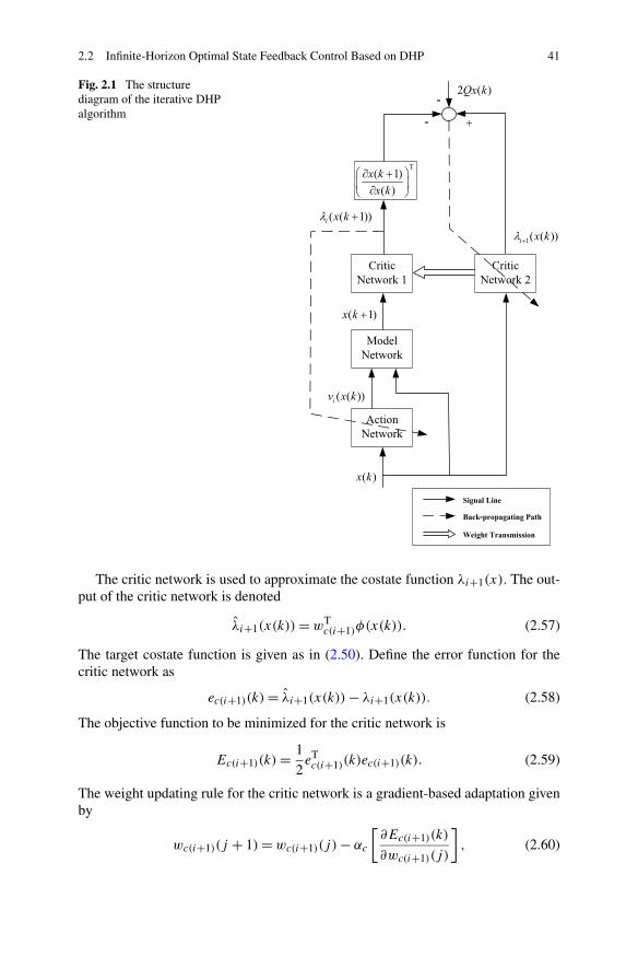
2.2 Infinite-Horizon Optimal State Feedback Control Based on DHP 41
Fig. 2.1 The structurediagram of the iterative DHPalgorithm
The critic network is used to approximate the costate function λi+1(x). The out-put of the critic network is denoted
λi+1(x(k))=wTc(i+1)φ(x(k)). (2.57)
The target costate function is given as in (2.50). Define the error function for thecritic network as
ec(i+1)(k)= λi+1(x(k))− λi+1(x(k)). (2.58)
The objective function to be minimized for the critic network is
Ec(i+1)(k)= 1
2eTc(i+1)(k)ec(i+1)(k). (2.59)
The weight updating rule for the critic network is a gradient-based adaptation givenby
wc(i+1)(j + 1)=wc(i+1)(j)− αc
[∂Ec(i+1)(k)
∂wc(i+1)(j)
], (2.60)
42 2 Optimal State Feedback Control for Discrete-Time Systems
where αc > 0 is the learning rate of the critic network, and j is the inner-loop itera-tion step for updating the weight parameters.
In the action network, the state x(k) is used as the input of the network and theoutput can be formulated as
vi (x(k))=wTaiφ(x(k)). (2.61)
The target value of the control vi(x(k)) is obtained by (2.46). So we can define theerror function of the action network as
eai(k)= vi (x(k))− vi(x(k)). (2.62)
The weights of the action network are updated to minimize the following perfor-mance error measure:
Eai(k)= 1
2eTai(k)eai(k). (2.63)
The updating algorithm is then similar to the one for the critic network. By thegradient descent rule, we obtain
wai(j + 1)=wai(j)− αa
[∂Eai(k)
∂wai(j)
], (2.64)
where αa > 0 is the learning rate of the action network, and j is the inner-loopiteration step for updating the weight parameters.
From the neural-network implementation, we can find that in this iterative DHPalgorithm, ∂Vi(x(k + 1))/∂x(k + 1) is replaced by λi (x(k + 1)), which is just theoutput of the critic network. Therefore, it is more accurate than computing by back-propagation through the critic network as in [1].
(3) Design procedure of the approximate optimal controller. Based on the itera-tive DHP algorithm, the design procedure of the optimal control scheme is summa-rized as follows:
1. Choose imax, jamax, jcmax, εm, ε0, U , αm, αc, αa and the weight matrices Q
and R.2. Construct the model network x(k + 1) = wT
mφ(Im(k)) with the initial weightparameters wm0 chosen randomly from [−0.1,0.1] and train the model networkwith a random input vector uniformly distributed in the interval [−1,1] andarbitrary initial state vector in [−1,1] till the given accuracy εm is reached.
3. Set the iteration step i = 0. Set the initial weight parameters of critic networkwc0 as zero so that the initial value of the costate function λ0(·) = 0, and ini-tialize the action network with the weight parameters wa0 chosen randomly in[−0.1,0.1].
4. Choose an array of state vector x(k) = (x(1)(k), x(2)(k), . . . , x(p)(k)) ran-domly from the operation region and compute the corresponding output targetvi(x(k))= (vi(x
(1)(k)), vi(x(2)(k)), . . . , vi(x
(p)(k))) by (2.46), where the state
2.2 Infinite-Horizon Optimal State Feedback Control Based on DHP 43
vector at the next time instant
x(k + 1)=(x(1)(k + 1), x(2)(k + 1), . . . , x(p)(k + 1)
)
is computed by the model network (2.53). With the same state vector x(k) =(x(1)(k), x(2)(k), . . . , x(p)(k)) and
x(k + 1)=(x(1)(k + 1), x(2)(k + 1), . . . , x(p)(k + 1)
),
compute the resultant output target
λi+1(x(k))=(λi+1(x
(1)(k)), λi+1(x(2)(k)), . . . , λi+1(x
(p)(k)))
by (2.50).5. Set wc(i+1) = wci . With the data set (x(j)(k), λi+1(x
(j)(k))), j = 1,2, . . . , p,update the weight parameters of the critic network wc(i+1) by (2.60) for jcmax
steps to get the approximate costate function λi+1.6. With the data set (x(j)(k), vi(x(j)(k))), j = 1,2, . . . , p, update the weight pa-
rameters of the action network wai by (2.64) for jamax steps to get the approxi-mate control law vi .
7. If
‖λi+1(x(k))− λi(x(k))‖2 < ε0,
go to Step 9; otherwise, go to Step 8.8. If i > imax, go to Step 9; otherwise, set i = i + 1 and go to Step 4.9. Set the final approximate optimal control law u∗(x)= vi (x).
10. Stop.
As stated in the last subsection, the iterative algorithm will be convergent withλi(x) → λ∗(x) and the control sequence vi(x) → u∗(x) as i → ∞. However, inpractical applications, we cannot implement the iteration till i → ∞. Actually, weiterate the algorithm for a max number imax or with a pre-specified accuracy ε0 totest the convergence of the algorithm. In the above procedure, there are two levelsof loops. The outer loop starts from Step 3 and ends at Step 8. There are two innerloops in Steps 5 and 6, respectively. The inner loop of Step 5 includes jcmax iterativesteps, and the inner loop of Step 6 includes jamax iterative steps. The state vectorx(k) is chosen randomly at Step 4. Suppose that the associated random probabilitydensity function is nonvanishing everywhere. Then we can assume that all the stateswill be explored. So we know that the resulting networks tend to satisfy the formulas(2.46) and (2.50) for all state vectors x(k). The limits of λi and vi will approximatethe optimal ones λ∗ and u∗, respectively. The parameters ε0 and imax are chosenby the designer. The smaller the value of ε0 is set, the more accurate the costatefunction and the optimal control law will be. If the condition set in Step 7 is satisfied,it implies that the costate function sequence is convergent with the pre-specified
44 2 Optimal State Feedback Control for Discrete-Time Systems
accuracy. The larger the value of imax in Step 8 is set, the more accurate the obtainedcontrol law v(x) will be at the price of increased computational burden.
2.2.3 Simulations
In this section, two examples are provided to demonstrate the effectiveness of thecontrol scheme developed in this subsection.
Example 2.9 (Nonlinear Discrete-Time System) Consider the following nonlinearsystem [5]:
x(k + 1)= f (x(k))+ g(x(k))u(k), (2.65)
where f (x(k)) = [ −0.8x2(k)
sin(0.8x1(k)−x2(k))+1.8x2(k)
], g(x(k)) = [ 0
−x2(k)
], and assume that
the control constraint is set to |u| ≤ 0.3.Define the cost functional as
J (x(k), u(·))=∞∑
i=k
{xT(i)Qx(i)+ 2
∫ u(i)
0tanh−T(U−1s)URds
}, (2.66)
where U = 0.3, and the weight matrices are chosen as Q= [ 1 00 1
]and R = [0.5].
First, we perform the simulation of iterative ADP algorithm. In this iterativealgorithm, we choose RBFNNs as the critic network, the action network and themodel network with the structure 2–9–2, 2–9–1 and 3–9–2, respectively. The train-ing sets are selected as −1 ≤ x1 ≤ 1 and −1 ≤ x2 ≤ 1, which is the operationregion of the system. It should be mentioned that the model network should betrained first. The initial state vectors are chosen randomly from [−1,1]. Under thelearning rate of αm = 0.1, the model network is trained until the given accuracyεm = 10−6 is reached. After the training of the model network is completed, theweights are kept unchanged. Then, the critic network and the action network aretrained with the learning rates αa = αc = 0.1 and the inner-loop iteration numberjcmax = jamax = 2000. Meanwhile the pre-specified accuracy ε0 is set to 10−20. De-note the outer loop iteration number as L. After implementing the outer loop itera-tion for L= imax = 100, the convergence curves of the costate function are shown inFig. 2.2. It can be seen that the costate function is basically convergent with the outerloop iteration L > 15. In order to compare the different actions of the control lawsobtained under different outer loop iteration numbers, for the same initial state vec-tor x1(0)= 0.5 and x2(0)= 0.5, we apply different control laws to the plant for 30time steps and obtain the simulation results as follows. The state curves are shownin Figs. 2.3 and 2.4, and the corresponding control inputs are shown in Fig. 2.5. Itcan be seen that the system responses are improved when the outer loop iterationnumber L is increased. When L > 80, the system responses only improve slightlyin performance.
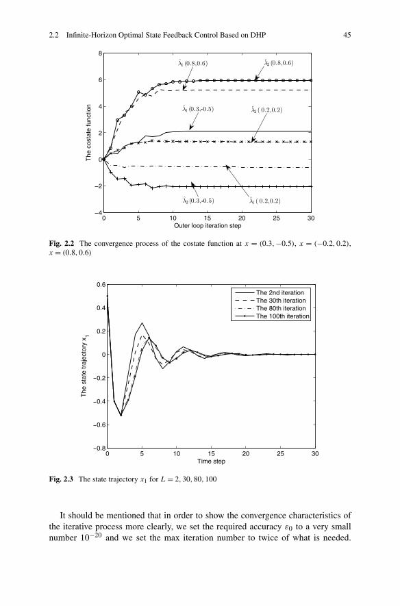
2.2 Infinite-Horizon Optimal State Feedback Control Based on DHP 45
Fig. 2.2 The convergence process of the costate function at x = (0.3,−0.5), x = (−0.2,0.2),x = (0.8,0.6)
Fig. 2.3 The state trajectory x1 for L= 2,30,80,100
It should be mentioned that in order to show the convergence characteristics ofthe iterative process more clearly, we set the required accuracy ε0 to a very smallnumber 10−20 and we set the max iteration number to twice of what is needed.
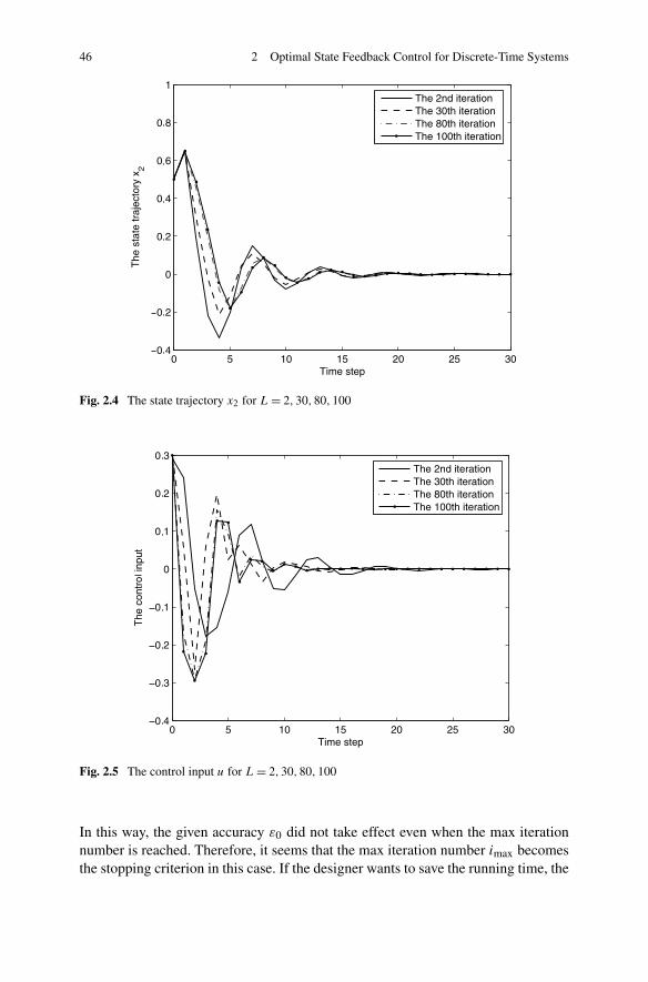
46 2 Optimal State Feedback Control for Discrete-Time Systems
Fig. 2.4 The state trajectory x2 for L= 2,30,80,100
Fig. 2.5 The control input u for L= 2,30,80,100
In this way, the given accuracy ε0 did not take effect even when the max iterationnumber is reached. Therefore, it seems that the max iteration number imax becomesthe stopping criterion in this case. If the designer wants to save the running time, the
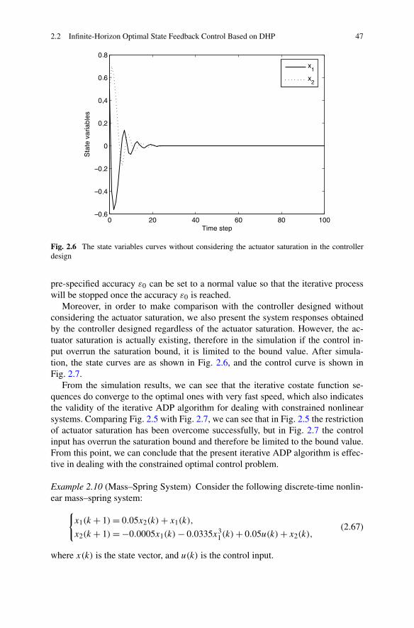
2.2 Infinite-Horizon Optimal State Feedback Control Based on DHP 47
Fig. 2.6 The state variables curves without considering the actuator saturation in the controllerdesign
pre-specified accuracy ε0 can be set to a normal value so that the iterative processwill be stopped once the accuracy ε0 is reached.
Moreover, in order to make comparison with the controller designed withoutconsidering the actuator saturation, we also present the system responses obtainedby the controller designed regardless of the actuator saturation. However, the ac-tuator saturation is actually existing, therefore in the simulation if the control in-put overrun the saturation bound, it is limited to the bound value. After simula-tion, the state curves are as shown in Fig. 2.6, and the control curve is shown inFig. 2.7.
From the simulation results, we can see that the iterative costate function se-quences do converge to the optimal ones with very fast speed, which also indicatesthe validity of the iterative ADP algorithm for dealing with constrained nonlinearsystems. Comparing Fig. 2.5 with Fig. 2.7, we can see that in Fig. 2.5 the restrictionof actuator saturation has been overcome successfully, but in Fig. 2.7 the controlinput has overrun the saturation bound and therefore be limited to the bound value.From this point, we can conclude that the present iterative ADP algorithm is effec-tive in dealing with the constrained optimal control problem.
Example 2.10 (Mass–Spring System) Consider the following discrete-time nonlin-ear mass–spring system:
{x1(k + 1)= 0.05x2(k)+ x1(k),
x2(k + 1)= −0.0005x1(k)− 0.0335x31(k)+ 0.05u(k)+ x2(k),
(2.67)
where x(k) is the state vector, and u(k) is the control input.
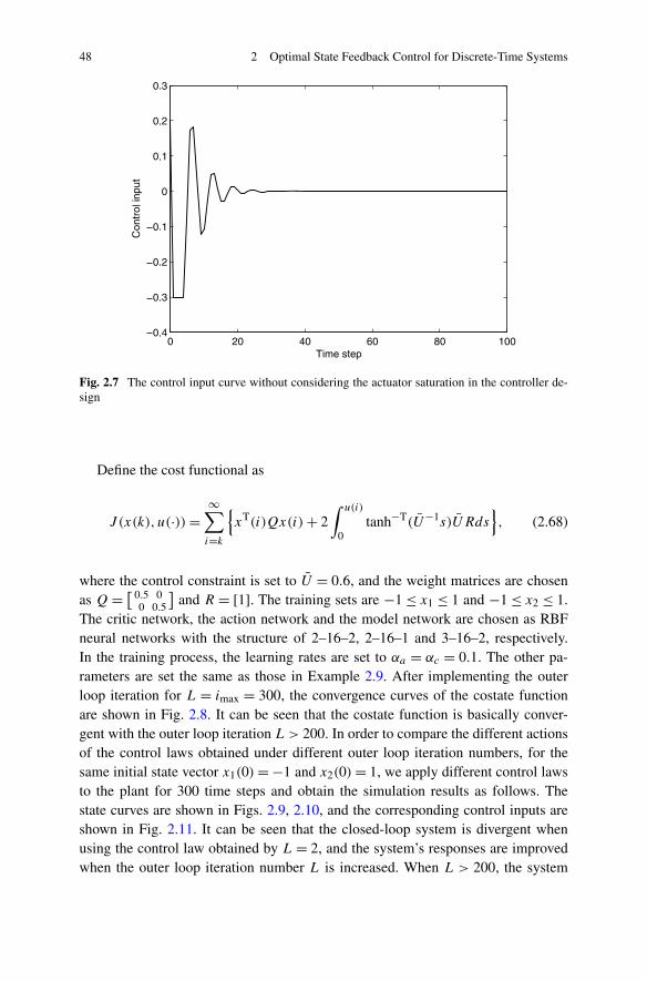
48 2 Optimal State Feedback Control for Discrete-Time Systems
Fig. 2.7 The control input curve without considering the actuator saturation in the controller de-sign
Define the cost functional as
J (x(k), u(·))=∞∑
i=k
{xT(i)Qx(i)+ 2
∫ u(i)
0tanh−T(U−1s)URds
}, (2.68)
where the control constraint is set to U = 0.6, and the weight matrices are chosenas Q = [ 0.5 0
0 0.5
]and R = [1]. The training sets are −1 ≤ x1 ≤ 1 and −1 ≤ x2 ≤ 1.
The critic network, the action network and the model network are chosen as RBFneural networks with the structure of 2–16–2, 2–16–1 and 3–16–2, respectively.In the training process, the learning rates are set to αa = αc = 0.1. The other pa-rameters are set the same as those in Example 2.9. After implementing the outerloop iteration for L = imax = 300, the convergence curves of the costate functionare shown in Fig. 2.8. It can be seen that the costate function is basically conver-gent with the outer loop iteration L> 200. In order to compare the different actionsof the control laws obtained under different outer loop iteration numbers, for thesame initial state vector x1(0)= −1 and x2(0)= 1, we apply different control lawsto the plant for 300 time steps and obtain the simulation results as follows. Thestate curves are shown in Figs. 2.9, 2.10, and the corresponding control inputs areshown in Fig. 2.11. It can be seen that the closed-loop system is divergent whenusing the control law obtained by L = 2, and the system’s responses are improvedwhen the outer loop iteration number L is increased. When L > 200, the system
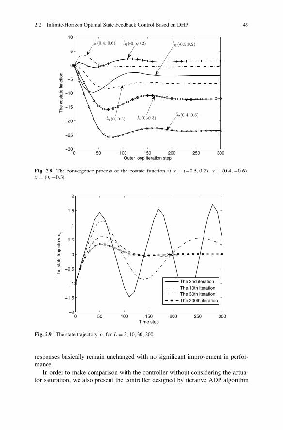
2.2 Infinite-Horizon Optimal State Feedback Control Based on DHP 49
Fig. 2.8 The convergence process of the costate function at x = (−0.5,0.2), x = (0.4,−0.6),x = (0,−0.3)
Fig. 2.9 The state trajectory x1 for L= 2,10,30,200
responses basically remain unchanged with no significant improvement in perfor-mance.
In order to make comparison with the controller without considering the actua-tor saturation, we also present the controller designed by iterative ADP algorithm
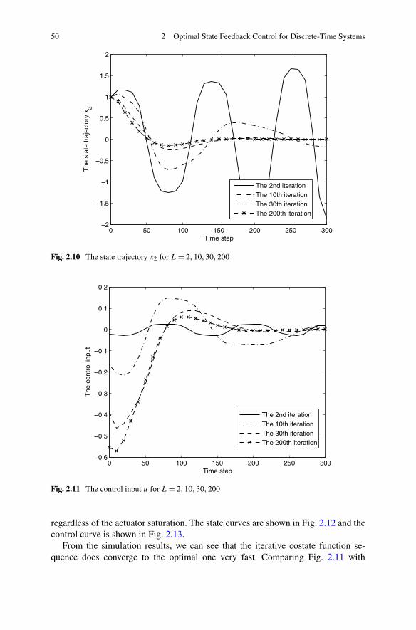
50 2 Optimal State Feedback Control for Discrete-Time Systems
Fig. 2.10 The state trajectory x2 for L= 2,10,30,200
Fig. 2.11 The control input u for L= 2,10,30,200
regardless of the actuator saturation. The state curves are shown in Fig. 2.12 and thecontrol curve is shown in Fig. 2.13.
From the simulation results, we can see that the iterative costate function se-quence does converge to the optimal one very fast. Comparing Fig. 2.11 with
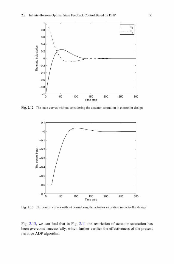
2.2 Infinite-Horizon Optimal State Feedback Control Based on DHP 51
Fig. 2.12 The state curves without considering the actuator saturation in controller design
Fig. 2.13 The control curves without considering the actuator saturation in controller design
Fig. 2.13, we can find that in Fig. 2.11 the restriction of actuator saturation hasbeen overcome successfully, which further verifies the effectiveness of the presentiterative ADP algorithm.
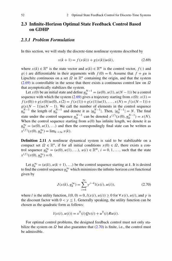
52 2 Optimal State Feedback Control for Discrete-Time Systems
2.3 Infinite-Horizon Optimal State Feedback Control Basedon GDHP
2.3.1 Problem Formulation
In this section, we will study the discrete-time nonlinear systems described by
x(k + 1)= f (x(k))+ g(x(k))u(k), (2.69)
where x(k) ∈ Rn is the state vector and u(k) ∈ R
m is the control vector, f (·) andg(·) are differentiable in their arguments with f (0) = 0. Assume that f + gu isLipschitz continuous on a set Ω in R
n containing the origin, and that the system(2.69) is controllable in the sense that there exists a continuous control law on Ω
that asymptotically stabilizes the system.Let x(0) be an initial state and define uN−1
0 = (u(0), u(1), u(N −1)) be a controlsequence with which the system (2.69) gives a trajectory starting from x(0): x(1)=f (x(0))+g(x(0))u(0), x(2)= f (x(1))+g(x(1))u(1), . . . , x(N)= f (x(N−1))+g(x(N − 1))u(N − 1). We call the number of elements in the control sequenceuN−1
0 the length of uN−10 and denote it as |uN−1
0 |. Then, |uN−10 | = N . The final
state under the control sequence uN−10 can be denoted x(f )(x(0), uN−1
0 ) = x(N).When the control sequence starting from u(0) has infinite length, we denote it asu∞
0 = (u(0), u(1), . . .) and then the correspondingly final state can be written asx(f )(x(0), u∞
0 )= limk→∞ x(k).
Definition 2.11 A nonlinear dynamical system is said to be stabilizable on acompact set Ω ∈ R
n, if for all initial conditions x(0) ∈ Ω , there exists a con-trol sequence u∞
0 = (u(0), u(1), . . .), u(i) ∈ Rm, i = 0,1, . . . , such that the state
x(f )(x(0), u∞0 )= 0.
Let u∞k = (u(k), u(k + 1), . . .) be the control sequence starting at k. It is desired
to find the control sequence u∞k which minimizes the infinite-horizon cost functional
given by
J (x(k), u∞k )=
∞∑
i=k
γ i−kl(x(i), u(i)), (2.70)
where l is the utility function, l(0,0)= 0, l(x(i), u(i))≥ 0 for ∀x(i), u(i), and γ isthe discount factor with 0 < γ ≤ 1. Generally speaking, the utility function can bechosen as the quadratic form as follows:
l(x(i), u(i))= xT(i)Qx(i)+ uT(i)Ru(i).
For optimal control problems, the designed feedback control must not only sta-bilize the system on Ω but also guarantee that (2.70) is finite, i.e., the control mustbe admissible.
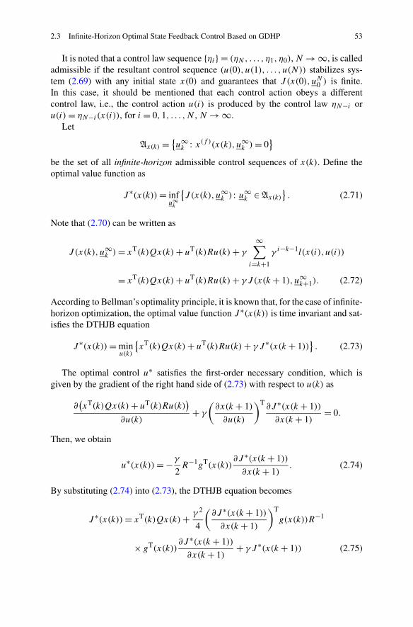
2.3 Infinite-Horizon Optimal State Feedback Control Based on GDHP 53
It is noted that a control law sequence {ηi} = (ηN , . . . , η1, η0), N → ∞, is calledadmissible if the resultant control sequence (u(0), u(1), . . . , u(N)) stabilizes sys-tem (2.69) with any initial state x(0) and guarantees that J (x(0), uN0 ) is finite.In this case, it should be mentioned that each control action obeys a differentcontrol law, i.e., the control action u(i) is produced by the control law ηN−i oru(i)= ηN−i (x(i)), for i = 0,1, . . . ,N , N → ∞.
Let
Ax(k) = {u∞k : x(f )(x(k), u∞
k )= 0}
be the set of all infinite-horizon admissible control sequences of x(k). Define theoptimal value function as
J ∗(x(k))= infu∞k
{J (x(k), u∞
k ) : u∞k ∈ Ax(k)
}. (2.71)
Note that (2.70) can be written as
J (x(k), u∞k )= xT(k)Qx(k)+ uT(k)Ru(k)+ γ
∞∑
i=k+1
γ i−k−1l(x(i), u(i))
= xT(k)Qx(k)+ uT(k)Ru(k)+ γ J (x(k + 1), u∞k+1). (2.72)
According to Bellman’s optimality principle, it is known that, for the case of infinite-horizon optimization, the optimal value function J ∗(x(k)) is time invariant and sat-isfies the DTHJB equation
J ∗(x(k))= minu(k)
{xT(k)Qx(k)+ uT(k)Ru(k)+ γ J ∗(x(k + 1))
}. (2.73)
The optimal control u∗ satisfies the first-order necessary condition, which isgiven by the gradient of the right hand side of (2.73) with respect to u(k) as
∂(xT(k)Qx(k)+ uT(k)Ru(k)
)
∂u(k)+ γ
(∂x(k + 1)
∂u(k)
)T∂J ∗(x(k + 1))
∂x(k + 1)= 0.
Then, we obtain
u∗(x(k))= −γ
2R−1gT(x(k))
∂J ∗(x(k + 1))
∂x(k + 1). (2.74)
By substituting (2.74) into (2.73), the DTHJB equation becomes
J ∗(x(k))= xT(k)Qx(k)+ γ 2
4
(∂J ∗(x(k + 1))
∂x(k + 1)
)T
g(x(k))R−1
× gT(x(k))∂J ∗(x(k + 1))
∂x(k + 1)+ γ J ∗(x(k + 1)) (2.75)
54 2 Optimal State Feedback Control for Discrete-Time Systems
where J ∗(x(k)) is the optimal value function corresponding to the optimal controllaw u∗(x(k)). When dealing with the linear quadratic regulator (LQR) optimal con-trol problems, this equation reduces to the Riccati equation which can be efficientlysolved. In the general nonlinear case, however, the HJB equation cannot be solvedexactly.
2.3.2 Infinite-Horizon Optimal State Feedback Control Basedon GDHP
Four parts are included in this subsection. In the first part, the unknown nonlinearsystem is identified via an NN system identification scheme with stability proof.The iterative ADP algorithm is introduced in the second part, while in the thirdpart, the corresponding convergence proof is developed. Then, in the fourth part,the implementation of the iterative ADP algorithm based on NN is described indetail.
2.3.2.1 NN Identification of the Unknown Nonlinear System
For the design of the NN identifier, a three-layer NN is considered as the functionapproximation structure. Let the number of hidden-layer neurons be denoted by l,the ideal weight matrix between the input layer and hidden layer be denoted by ν∗
m,and the ideal weight matrix between the hidden layer and output layer be denotedby ω∗
m. According to the universal approximation property [8] of NN, the systemdynamics (2.69) has a NN representation on a compact set S, which can be writtenas
x(k + 1)= ω∗Tm σ
(ν∗Tm z(k)
)+ θ(k). (2.76)
In (2.76), z(k) = [xT(k) uT(k)]T is the NN input, θ(k) is the bounded NN func-tional approximation error according to the universal approximation property, and[σ(z)]i = (ezi − e−zi )/(ezi + e−zi ), i = 1,2, . . . , l, are the activation functions se-lected in this work, where z(k) = ν∗T
m z(k), z(k) ∈ Rl . Additionally, the NN activa-
tion functions are bounded such that ‖σ(z(k))‖ ≤ σM for a constant σM .In the system identification process, we keep the weight matrix between the input
layer and the hidden layer as constant while only tune the weight matrix betweenthe hidden layer and the output layer. So, we define the NN system identificationscheme as
x(k + 1)= ωTm(k)σ (z(k)), (2.77)
where x(k) is the estimated system state vector, and ωm(k) is the estimation of theconstant ideal weight matrix ω∗
m.
2.3 Infinite-Horizon Optimal State Feedback Control Based on GDHP 55
Denote x(k)= x(k)− x(k) as the system identification error. Combining (2.76)and (2.77), we can obtain the identification error dynamics as
x(k + 1)= ωTm(k)σ (z(k))− θ(k), (2.78)
where ωm(k)= ωm(k)−ω∗m. Let ψ(k)= ωT
m(k)σ (z(k)). Then, (2.78) can be rewrit-ten as
x(k + 1)=ψ(k)− θ(k). (2.79)
The weights in the system identification process are updated to minimize thefollowing performance measure:
E(k + 1)= 1
2xT(k + 1)x(k + 1). (2.80)
Using the gradient-based adaptation rule, the weights can be updated as
ωm(k + 1)= ωm(k)− αm
[∂E(k + 1)
∂ωm(k)
]
= ωm(k)− αmσ(z(k))xT(k + 1), (2.81)
where αm > 0 is the NN learning rate.We now give the following assumption before presenting the asymptotic stability
proof of the state estimation error x(k).
Assumption 2.12 The NN approximation error term θ(k) is assumed to be upperbounded by a function of the state estimation error x(k) such that
θT(k)θ(k)≤ θMk = δxT(k)x(k), (2.82)
where δ is the constant target value with δM as its upper bound, i.e., ‖δ‖ ≤ δM .
Next, the stability analysis of the present NN-based system identification schemeis presented by using the Lyapunov theory.
Theorem 2.13 (cf. [10]) Let the identification scheme (2.77) be used to identifythe nonlinear system (2.69), and let the parameter update law given in (2.81) beused for tuning the NN weights. Then, the state estimation error dynamics x(k) isasymptotically stable while the parameter estimation error ωm(k) is bounded.
Proof Consider the following positive definite Lyapunov function candidate:
Lk = L1k +L2k, (2.83)
where
L1k = xT(k)x(k),
56 2 Optimal State Feedback Control for Discrete-Time Systems
L2k = 1
αmtr{ωTm(k)ωm(k)
}.
Taking the first difference of the Lyapunov function (2.83) and substituting the iden-tification error dynamics (2.79) and the NN weight update law (2.81) reveal that
ΔL1k = xT(k + 1)x(k + 1)− xT(k)x(k)
=ψT(k)ψ(k)− 2ψT(k)θ(k)+ θT(k)θ(k)− xT(k)x(k)
ΔL2k = 1
αmtr{ωTm(k + 1)ωm(k + 1)− ωT
m(k)ωm(k)}
= 1
αmtr{− 2αmψ(k)x
T(k + 1)
+ α2mx(k + 1)σT(z(k))σ (z(k))xT(k + 1)
}
= −2ψT(k)x(k + 1)+ αmσT(z(k))σ (z(k))xT(k + 1)x(k + 1).
After applying the Cauchy–Schwarz inequality ((a1 + a2 + · · · + an)T(a1 + a2 +
· · · + an)≤ n(aT1 a1 + aT
2 a2 + · · · + aTn an)) to ΔL2k , we have
ΔL2k ≤ −2ψT(k)(ψ(k)− θ(k))
+ 2αmσT(z(k))σ (z(k))
(ψT(k)ψ(k)+ θT(k)θ(k)
).
Therefore, we can find that
ΔLk ≤ −ψT(k)ψ(k)+ θT(k)θ(k)− xT(k)x(k)
+ 2αmσT(z(k))σ (z(k))
(ψT(k)ψ(k)+ θT(k)θ(k)
).
Considering ‖σ(z(k))‖ ≤ σM and (2.82), we obtain
ΔLk ≤ −(1 − 2αmσ2M
)‖ψ(k)‖2
− (1 − δM − 2αmδMσ 2
M
)‖x(k)‖2. (2.84)
Define αm ≤ ρ2/(2σ 2M); then (2.84) becomes
ΔLk ≤ −(1 − ρ2)‖ψ(k)‖2 − (1 − δM − δMρ2)‖x(k)‖2
= −(1 − ρ2)∥∥ωTm(k)σ (z(k))
∥∥2
− (1 − δM − δMρ2)‖x(k)‖2. (2.85)
From (2.85), we can conclude that ΔLk ≤ 0 provided 0 < δM < 1 and
max
{−√
1 − δM
δM,−1
}≤ ρ ≤ min
{√1 − δM
δM,1
},
2.3 Infinite-Horizon Optimal State Feedback Control Based on GDHP 57
where ρ �= 0. As long as the parameters are selected as discussed above, ΔLk ≤ 0 in(2.85), which shows stability in the sense of Lyapunov. Therefore, x(k) and ωm(k)
are bounded, provided x0 and ωm(0) are bounded in the compact set S. Furthermore,by summing both sides of (2.85) to infinity and taking account of ΔLk ≤ 0, we have
∣∣∣∣∣
∞∑
k=0
ΔLk
∣∣∣∣∣=∣∣∣ limk→∞Lk −L0
∣∣∣<∞.
This implies that
∞∑
k=0
{(1 − ρ2)∥∥ωT
m(k)σ (z(k))∥∥2 + (
1 − δM − δMρ2)‖x(k)‖2}<∞.
Hence, it can be concluded that the estimation error approaches zero, i.e.,‖x(k)‖ → 0 as k → ∞. �
Remark 2.14 According to Theorem 2.13, after a sufficient learning session, the NNsystem identification error converges to zero, i.e., we have
f (x(k))+ g(x(k))u(k)= ωTm(k)σ (z(k)), (2.86)
where g(x(k)) denotes the estimated value of the control coefficient matrix g(x(k)).Taking the partial derivative of both sides of (2.86) with respect to u(k) yields
g(x(k))= ∂(ωTm(k)σ (z(k))
)
∂u(k)
= ωTm(k)
∂σ (z(k))
∂z(k)ν∗Tm
∂z(k)
∂u(k), (2.87)
where
∂z(k)
∂u(k)=[
0n×m
Im
],
and Im is the m×m identity matrix.
Next, this result will be used in the derivation and implementation of the iterativeADP algorithm for the optimal control of unknown discrete-time nonlinear systems.
2.3.2.2 Derivation of the Iterative ADP Algorithm
In this part, we mainly present the iterative ADP algorithm. First, we start with theinitial value function V0(·) = 0, and then solve for the law of single control vectorv0(x(k)) as follows:
v0(x(k))= arg minu(k)
{xT(k)Qx(k)+ uT(k)Ru(k)+ γV0(x(k + 1))
}. (2.88)
58 2 Optimal State Feedback Control for Discrete-Time Systems
Once the control law v0(x(k)) is determined, we update the cost function as
V1(x(k))= minu(k)
{xT(k)Qx(k)+ uT(k)Ru(k)+ γV0(x(k + 1))
}
= xT(k)Qx(k)+ vT0 (x(k))Rv0(x(k)). (2.89)
Therefore, for i = 1,2, . . . , the iterative ADP algorithm can be used to implementthe iteration between the control law
vi(x(k))= arg minu(k)
{xT(k)Qx(k)+ uT(k)Ru(k)+ γVi(x(k + 1))
}
= −γ
2R−1gT(x(k))
∂Vi(x(k + 1))
∂x(k + 1)(2.90)
and the value function
Vi+1(x(k))= minu(k)
{xT(k)Qx(k)+ uT(k)Ru(k)+ γVi(x(k + 1))
}
= xT(k)Qx(k)+ vTi (x(k))Rvi(x(k))+ γVi(x(k + 1)). (2.91)
In the above recurrent iteration, i is the iteration index of the control law andvalue function, while k is the time index of the system’s control and state trajec-tories. The value function and control law are updated until they converge to theoptimal ones. In the following part, we will present a proof of convergence of theiteration between (2.90) and (2.91) with the value function Vi → J ∗ and the controllaw vi → u∗ as i → ∞.
2.3.2.3 Convergence Analysis of the Iterative ADP Algorithm
Lemma 2.15 Let {μi} be an arbitrary sequence of control laws and {vi} be thecontrol law sequence described in (2.90). Define Vi as in (2.91) and Λi as
Λi+1(x(k))= xT(k)Qx(k)+μTi (x(k))Rμi(x(k))+ γΛi(x(k + 1)). (2.92)
If V0(x(k))=Λ0(x(k))= 0, then Vi(x(k))≤Λi(x(k)), ∀i.
Proof It can easily be derived noticing that Vi+1 is the result of minimizing the righthand side of (2.91) with respect to the control input u(k), while Λi+1 is a result ofarbitrary control input. �
Lemma 2.16 Let the value function sequence {Vi} be defined as in (2.91). If thesystem is controllable, then there is an upper bound Y such that 0 ≤ Vi(x(k))≤ Y ,∀i.
2.3 Infinite-Horizon Optimal State Feedback Control Based on GDHP 59
Proof Let {ηi(x)} be a sequence of admissible control laws, and let V0(·)= Z0(·)=0, where Vi is updated as in (2.91) and Zi is updated by
Zi+1(x(k))= xT(k)Qx(k)+ ηTi (x(k))Rηi(x(k))+ γZi(x(k + 1)). (2.93)
It is clear that
Zi(x(k + 1))= xT(k + 1)Qx(k + 1)+ ηTi−1(x(k + 1))Rηi−1(x(k + 1))
+ γZi−1(x(k + 2)). (2.94)
Noticing that l(x(k), ηi(x(k)))= xT(k)Qx(k)+ηTi (x(k))Rηi(x(k)), we can further
obtain
Zi+1(x(k))= l(x(k), ηi(x(k)))+ γ l(x(k + 1), ηi−1(x(k + 1)))
+ γ 2Zi−1(x(k + 2))
= l(x(k), ηi(x(k)))+ γ l(x(k + 1), ηi−1(x(k + 1)))
+ γ 2l(x(k + 2), ηi−2(x(k + 2)))+ γ 3Zi−2(x(k + 3))
...
= l(x(k), ηi(x(k)))+ γ l(x(k + 1), ηi−1(x(k + 1)))
+ γ 2l(x(k + 2), ηi−2(x(k + 2)))
+ · · · + γ il(x(k + i), η0(x(k + i)))
+ γ i+1Z0(x(k + i + 1)), (2.95)
where Z0(x(k + i + 1))= 0. Then, (2.95) can be written as
Zi+1(x(k))=i∑
j=0
γ j l(x(k + j), ηi−j (x(k + j)))
=i∑
j=0
γ j(xT(k + j)Qx(k + j)+ ηT
i−j (x(k + j))Rηi−j (x(k + j)))
≤ limi→∞
i∑
j=0
γ j(xT(k + j)Qx(k + j)
+ ηTi−j (x(k + j))Rηi−j (x(k + j))
). (2.96)
60 2 Optimal State Feedback Control for Discrete-Time Systems
Since {ηi(x)} is an admissible control law sequence, we have x(k)→ 0 as k → ∞,and there exists an upper bound Y such that
Zi+1(x(k))≤ limi→∞
i∑
j=0
γ j l(x(k + j), ηi−j (x(k + j)))≤ Y, ∀i. (2.97)
By using Lemma 2.15, we obtain
Vi+1(x(k))≤Zi+1(x(k))≤ Y, ∀i. (2.98)
�
Based on Lemmas 2.15 and 2.16, we now present our main theorems.
Theorem 2.17 Define the value function sequence {Vi} as in (2.91) with V0(·) =0, and the control law sequence {vi} as in (2.90). Then, {Vi} is a monotonicallynondecreasing sequence satisfying Vi+1 ≥ Vi , ∀i.
Proof Define a new sequence
Φi+1(x(k))= xT(k)Qx(k)+ vTi+1(x(k))Rvi+1(x(k))+ γΦi(x(k + 1)) (2.99)
with Φ0(·) = V0(·) = 0. Let the control law sequence {vi} and the value functionsequence {Vi} be updated as in (2.90) and (2.91), respectively.
In the following part, we prove that Φi(x(k)) ≤ Vi+1(x(k)) by mathematicalinduction.
First, we prove that it holds for i = 0. Considering
V1(x(k))−Φ0(x(k))= xT(k)Qx(k)+ vT0 (x(k))Rv0(x(k))≥ 0
then, for i = 0, we get
V1(x(k))≥Φ0(x(k)). (2.100)
Second, we assume that it holds for i−1, i.e., Vi(x(k))≥Φi−1(x(k)), ∀x(k). Then,for i, noticing that
Vi+1(x(k))= xT(k)Qx(k)+ vTi (x(k))Rvi(x(k))+ γVi(x(k + 1))
and
Φi(x(k))= xT(k)Qx(k)+ vTi (x(k))Rvi(x(k))+ γΦi−1(x(k + 1)),
we get
Vi+1(x(k))−Φi(x(k))= γ (Vi(x(k + 1))−Φi−1(x(k + 1)))≥ 0
2.3 Infinite-Horizon Optimal State Feedback Control Based on GDHP 61
i.e.,
Vi+1(x(k))≥Φi(x(k)). (2.101)
Thus, we complete the proof through mathematical induction.Furthermore, from Lemma 2.15 we know that Vi(x(k)) ≤ Φi(x(k)), therefore,
we have
Vi+1(x(k))≥Φi(x(k))≥ Vi(x(k)). (2.102)
�
We have reached the conclusion that the value function sequence {Vi} is a mono-tonically nondecreasing sequence with an upper bound, and therefore, its limit ex-ists. Now, we can derive the following theorem.
Theorem 2.18 For any state vector x(k), define
limi→∞Vi(x(k))= V∞(x(k))
as the limit of the value function sequence {Vi}. Then, the following equation holds:
V∞(x(k))= minu(k)
{xT(k)Qx(k)+ uT(k)Ru(k)+ γV∞(x(k + 1))
}.
Proof For any u(k) and i, according to (2.91), we can derive
Vi(x(k))≤ xT(k)Qx(k)+ uT(k)Ru(k)+ γVi−1(x(k + 1)).
Combining with
Vi(x(k))≤ V∞(x(k)), ∀i (2.103)
which is obtained from Theorem 2.17, we have
Vi(x(k))≤ xT(k)Qx(k)+ uT(k)Ru(k)+ γV∞(x(k + 1)), ∀i.Let i → ∞, we can acquire
V∞(x(k))≤ xT(k)Qx(k)+ uT(k)Ru(k)+ γV∞(x(k + 1)).
Note that in the above equation, u(k) is chosen arbitrarily; thus, we obtain
V∞(x(k))≤ minu(k)
{xT(k)Qx(k)+ uT(k)Ru(k)+ γV∞(x(k + 1))
}. (2.104)
On the other hand, since the value function sequence satisfies
Vi(x(k))= minu(k)
{xT(k)Qx(k)+ uT(k)Ru(k)+ γVi−1(x(k + 1))
}
62 2 Optimal State Feedback Control for Discrete-Time Systems
for any i, considering (2.103), we have
V∞(x(k))≥ minu(k)
{xT(k)Qx(k)+ uT(k)Ru(k)+ γVi−1(x(k + 1))
}, ∀i.
Let i → ∞; we get
V∞(x(k))≥ minu(k)
{xT(k)Qx(k)+ uT(k)Ru(k)+ γV∞(x(k + 1))
}. (2.105)
Based on (2.104) and (2.105), we can acquire the conclusion that V∞(x(k)) =minu(k){xT(k)Qx(k)+ uT(k)Ru(k)+ γV∞(x(k + 1))}. �
Next, we will prove that the value function sequence {Vi} converges to the opti-mal value function J ∗(x(k)) as i → ∞.
Theorem 2.19 (cf. [10]) Define the value function sequence {Vi} as in (2.91) withV0(·) = 0. If the system state x(k) is controllable, then J ∗ is the limit of the valuefunction sequence {Vi}, i.e.,
limi→∞Vi(x(k))= J ∗(x(k)).
Proof Let {η(l)i } be the lth admissible control law sequence. We construct the asso-
ciated sequence {P (l)i (x)} as follows:
P(l)i+1(x(k))= xT(k)Qx(k)+ η
(l)Ti (x(k))Rη
(l)i (x(k))+ γP
(l)i (x(k + 1)) (2.106)
with P(l)0 (·)= 0. Similar to the derivation of (2.95), we get
P(l)i+1(x(k))=
i∑
j=0
γ j l(x(k + j), η
(l)i−j (x(k + j))
). (2.107)
Using Lemmas 2.15 and 2.16, we have
Vi+1(x(k))≤ P(l)i+1(x(k))≤ Yl, ∀l, i (2.108)
where Yl is the upper bound associated with the sequence {P (l)i+1(x(k))}. Denote
limi→∞P
(l)i (x(k))= P (l)∞ (x(k));
then, we obtain
V∞(x(k))≤ P (l)∞ (x(k))≤ Yl, ∀l. (2.109)
2.3 Infinite-Horizon Optimal State Feedback Control Based on GDHP 63
Let the corresponding control sequence associated with (2.107) be
(l)uk+ik = (
(l)u(k),(l) u(k + 1), . . . ,(l) uk+i
)
= (η(l)i (x(k)), η
(l)i−1(x(k + 1)), . . . , η(l)0 (x(k + i))
);then we have
J(x(k),(l) u
k+ik
)=i∑
j=0
γ j l(x(k + j), η
(l)i−j (x(k + j))
)= P(l)i+1(x(k)). (2.110)
Letting i → ∞, and denoting the admissible control sequence related to P(l)∞(x(k))
with length ∞ as (l)u∞k , we get
J(x(k),(l) u
∞k
)=∞∑
j=0
γ j l(x(k + j),(l) u(k + j)
)= P (l)∞ (x(k)). (2.111)
Then, according to the definition of J ∗(x(k)) in (2.71), for any ε > 0, there exists asequence of admissible control laws {η(M)
i } such that the associated cost function
J(x(k),(M) u
∞k
)=∞∑
j=0
γ j l(x(k + j),(M) u(k + j)
)= P (M)∞ (x(k)) (2.112)
satisfies J (x(k),(M) u∞k )≤ J ∗(x(k))+ ε. Combining with (2.109), we have
V∞(x(k))≤ P (M)∞ (x(k))≤ J ∗(x(k))+ ε. (2.113)
Since ε is chosen arbitrarily, we get
V∞(x(k))≤ J ∗(x(k)). (2.114)
On the other hand, because Vi+1(x(k)) ≤ P(l)i+1(x(k)) ≤ Yl,∀l, i, we can get
V∞(x(k)) ≤ infl{Yl}. According to the definition of admissible control law se-quence, the control law sequence associated with the cost function V∞(x(k)) mustbe an admissible control law sequence. We can see that there exists a sequence ofadmissible control laws {η(N)
i } such that V∞(x(k))= P(N)∞ (x(k)). Combining with
(2.111), we get V∞(x(k)) = J (x(k),(N) u∞k ). Sine J ∗(x(k)) is the infimum of all
admissible control sequences starting at k with length ∞, we obtain
V∞(x(k))≥ J ∗(x(k)). (2.115)
Based on (2.114) and (2.115), we can conclude that J ∗ is the limit of the valuefunction sequence {Vi}, i.e., V∞(x(k))= J ∗(x(k)). �
From Theorems 2.17 and 2.18, we can derive that the limit of the value functionsequence {Vi} satisfies the DTHJB equation, i.e., V∞(x(k))= minu(k){xT(k)Qx(k)
64 2 Optimal State Feedback Control for Discrete-Time Systems
+ uT(k)Ru(k) + γV∞(x(k + 1))}. Besides, from Theorem 2.19, we can get theresult that V∞(x(k)) = J ∗(x(k)). Therefore, we can find that the cost function se-quence {Vi(x(k))} converges to the optimal value function J ∗(x(k)) of the DTHJBequation, i.e., Vi → J ∗ as i → ∞. Then, according to (2.74) and (2.90), we can con-clude the convergence of the corresponding control law sequence. Now, we presentthe following corollary.
Corollary 2.20 Define the value function sequence {Vi} as in (2.91) with V0(·)= 0,and the control law sequence {vi} as in (2.90). If the system state x(k) is control-lable, then the sequence {vi} converges to the optimal control law u∗ as i → ∞,i.e.,
limi→∞vi(x(k))= u∗(x(k)).
Remark 2.21 Like (2.95), when we further expand (2.91), we obtain a control lawsequence (vi, vi−1, . . . , v0) and the resultant control sequence (vi(x(0)), vi−1(x(1)),. . . , v0(x(i))). With the iteration number increasing to ∞, the derived control lawsequence has the length of ∞. Then, using the corresponding control sequence, weobtain a state trajectory. However, it is not derived from a single control law. Forinfinite-horizon optimal control problem, what we should get is a unique optimalcontrol law under which we can obtain the optimal state trajectory. Therefore, weonly use the optimal control law u∗ obtained in Corollary 2.20 to produce a controlsequence when we apply the algorithm to practical systems.
2.3.2.4 NN Implementation of the Iterative ADP Algorithm Using GDHPTechnique
When the controlled system is linear and the cost function is quadratic, we canobtain a linear control law. In the nonlinear case, however, this is not necessarilytrue. Therefore, we need to use function approximation structure, such as NN, toapproximate both vi(x(k)) and Vi(x(k)).
Now, we implement the iterative GDHP algorithm in (2.90) and (2.91). In theiterative GDHP algorithm, there are three networks, which are model network, criticnetwork and action network. All the networks are chosen as three-layer feedforwardNNs. The input of the critic network and action network is x(k), while the inputof the model network is x(k) and vi (x(k)). The diagram of the whole structure isshown in Fig. 2.14, where
DER =(∂x(k + 1)
∂x(k)+ ∂x(k + 1)
∂vi(x(k))
∂vi(x(k))
∂x(k)
)T
.
The training of the model network is completed after the system identificationprocess and its weights are kept unchanged. Then, according to Theorem 2.13, whengiven x(k) and vi (x(k)), we can compute x(k + 1) by (2.77), i.e.,
x(k + 1)= ωTm(k)σ
(ν∗Tm [xT(k) vT
i (x(k))]T).
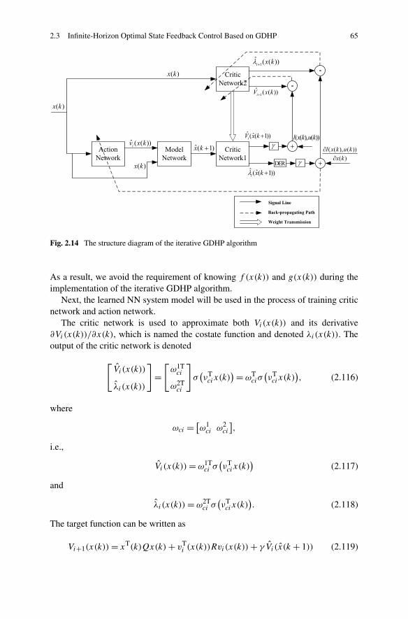
2.3 Infinite-Horizon Optimal State Feedback Control Based on GDHP 65
Fig. 2.14 The structure diagram of the iterative GDHP algorithm
As a result, we avoid the requirement of knowing f (x(k)) and g(x(k)) during theimplementation of the iterative GDHP algorithm.
Next, the learned NN system model will be used in the process of training criticnetwork and action network.
The critic network is used to approximate both Vi(x(k)) and its derivative∂Vi(x(k))/∂x(k), which is named the costate function and denoted λi(x(k)). Theoutput of the critic network is denoted
[Vi(x(k))
λi(x(k))
]=[ω1Tci
ω2Tci
]σ(νTcix(k)
)= ωTciσ
(νTcix(k)
), (2.116)
where
ωci = [ω1ci ω2
ci
],
i.e.,
Vi (x(k))= ω1Tci σ
(νTcix(k)
)(2.117)
and
λi (x(k))= ω2Tci σ
(νTcix(k)
). (2.118)
The target function can be written as
Vi+1(x(k))= xT(k)Qx(k)+ vTi (x(k))Rvi(x(k))+ γ Vi(x(k + 1)) (2.119)
66 2 Optimal State Feedback Control for Discrete-Time Systems
and
λi+1(x(k))= ∂(xT(k)Qx(k)+ vT
i (x(k))Rvi(x(k)))
∂x(k)+ γ
∂Vi(x(k + 1))
∂x(k)
= 2Qx(k)+ 2
(∂vi(x(k))
∂x(k)
)T
Rvi(x(k))
+ γ
(∂x(k + 1)
∂x(k)+ ∂x(k + 1)
∂vi(x(k))
∂vi(x(k))
∂x(k)
)T
λi (x(k + 1)). (2.120)
Then, we define the error function for training the critic network as
e1cik = Vi (x(k))− Vi+1(x(k)) (2.121)
and
e2cik = λi (x(k))− λi+1(x(k)). (2.122)
The objective function to be minimized in the critic network training is
Ecik = (1 − β)E1cik + βE2
cik, (2.123)
where
E1cik = 1
2e1Tcike
1cik (2.124)
and
E2cik = 1
2e2Tcike
2cik. (2.125)
The weight updating rule for training the critic network is also gradient-based adap-tation given by
ωci(j + 1)= ωci(j)− αc
[(1 − β)
∂E1cik
∂ωci(j)+ β
∂E2cik
∂ωci(j)
](2.126)
νci(j + 1)= νci(j)− αc
[(1 − β)
∂E1cik
∂νci(j)+ β
∂E2cik
∂νci(j)
](2.127)
where αc > 0 is the learning rate of the critic network, j is the inner-loop iterationstep for updating the weight parameters, and 0 ≤ β ≤ 1 is a parameter that adjustshow HDP and DHP are combined in GDHP. For β = 0, the training of the criticnetwork reduces to a pure HDP, while β = 1 does the same for DHP.
In the action network, the state x(k) is used as input to obtain the optimal control.The output can be formulated as
vi (x(k))= ωTaiσ
(νTaix(k)
). (2.128)
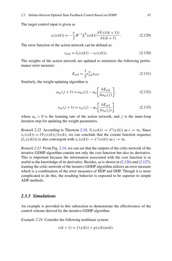
2.3 Infinite-Horizon Optimal State Feedback Control Based on GDHP 67
The target control input is given as
vi(x(k))= −γ
2R−1gT(x(k))
∂Vi(x(k + 1))
∂x(k + 1). (2.129)
The error function of the action network can be defined as
eaik = vi (x(k))− vi(x(k)). (2.130)
The weights of the action network are updated to minimize the following perfor-mance error measure:
Eaik = 1
2eTaikeaik. (2.131)
Similarly, the weight updating algorithm is
ωai(j + 1)= ωai(j)− αa
[∂Eaik
∂ωai(j)
], (2.132)
νai(j + 1)= νai(j)− αa
[∂Eaik
∂νai(j)
](2.133)
where αa > 0 is the learning rate of the action network, and j is the inner-loopiteration step for updating the weight parameters.
Remark 2.22 According to Theorem 2.19, Vi(x(k)) → J ∗(x(k)) as i → ∞. Sinceλi(x(k)) = ∂Vi(x(k))/∂x(k), we can conclude that the costate function sequence{λi(x(k))} is also convergent with λi(x(k))→ λ∗(x(k)) as i → ∞.
Remark 2.23 From Fig. 2.14, we can see that the outputs of the critic network of theiterative GDHP algorithm contain not only the cost function but also its derivative.This is important because the information associated with the cost function is asuseful as the knowledge of its derivative. Besides, as is shown in (2.126) and (2.127),training the critic network of the iterative GDHP algorithm utilizes an error measurewhich is a combination of the error measures of HDP and DHP. Though it is morecomplicated to do this, the resulting behavior is expected to be superior to simpleADP methods.
2.3.3 Simulations
An example is provided in this subsection to demonstrate the effectiveness of thecontrol scheme derived by the iterative GDHP algorithm.
Example 2.24 Consider the following nonlinear system:
x(k + 1)= f (x(k))+ g(x(k))u(k),
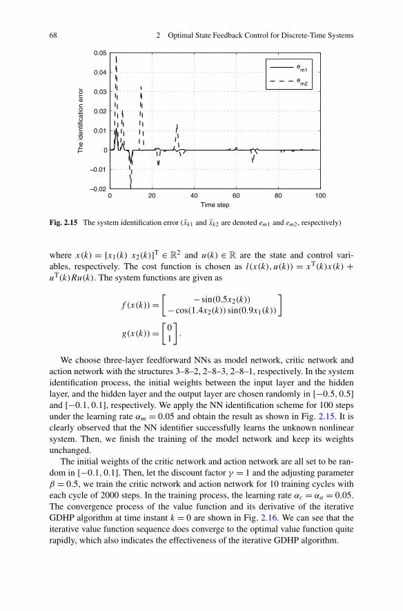
68 2 Optimal State Feedback Control for Discrete-Time Systems
Fig. 2.15 The system identification error (xk1 and xk2 are denoted em1 and em2, respectively)
where x(k) = [x1(k) x2(k)]T ∈ R2 and u(k) ∈ R are the state and control vari-
ables, respectively. The cost function is chosen as l(x(k), u(k)) = xT(k)x(k) +uT(k)Ru(k). The system functions are given as
f (x(k))=[ − sin(0.5x2(k))
− cos(1.4x2(k)) sin(0.9x1(k))
]
g(x(k))=[
01
].
We choose three-layer feedforward NNs as model network, critic network andaction network with the structures 3–8–2, 2–8–3, 2–8–1, respectively. In the systemidentification process, the initial weights between the input layer and the hiddenlayer, and the hidden layer and the output layer are chosen randomly in [−0.5,0.5]and [−0.1,0.1], respectively. We apply the NN identification scheme for 100 stepsunder the learning rate αm = 0.05 and obtain the result as shown in Fig. 2.15. It isclearly observed that the NN identifier successfully learns the unknown nonlinearsystem. Then, we finish the training of the model network and keep its weightsunchanged.
The initial weights of the critic network and action network are all set to be ran-dom in [−0.1,0.1]. Then, let the discount factor γ = 1 and the adjusting parameterβ = 0.5, we train the critic network and action network for 10 training cycles witheach cycle of 2000 steps. In the training process, the learning rate αc = αa = 0.05.The convergence process of the value function and its derivative of the iterativeGDHP algorithm at time instant k = 0 are shown in Fig. 2.16. We can see that theiterative value function sequence does converge to the optimal value function quiterapidly, which also indicates the effectiveness of the iterative GDHP algorithm.
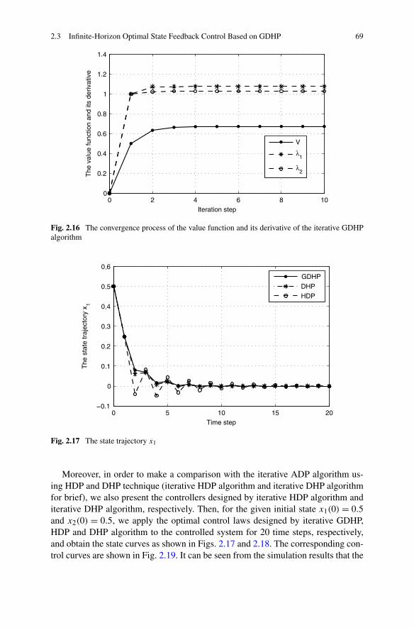
2.3 Infinite-Horizon Optimal State Feedback Control Based on GDHP 69
Fig. 2.16 The convergence process of the value function and its derivative of the iterative GDHPalgorithm
Fig. 2.17 The state trajectory x1
Moreover, in order to make a comparison with the iterative ADP algorithm us-ing HDP and DHP technique (iterative HDP algorithm and iterative DHP algorithmfor brief), we also present the controllers designed by iterative HDP algorithm anditerative DHP algorithm, respectively. Then, for the given initial state x1(0) = 0.5and x2(0) = 0.5, we apply the optimal control laws designed by iterative GDHP,HDP and DHP algorithm to the controlled system for 20 time steps, respectively,and obtain the state curves as shown in Figs. 2.17 and 2.18. The corresponding con-trol curves are shown in Fig. 2.19. It can be seen from the simulation results that the
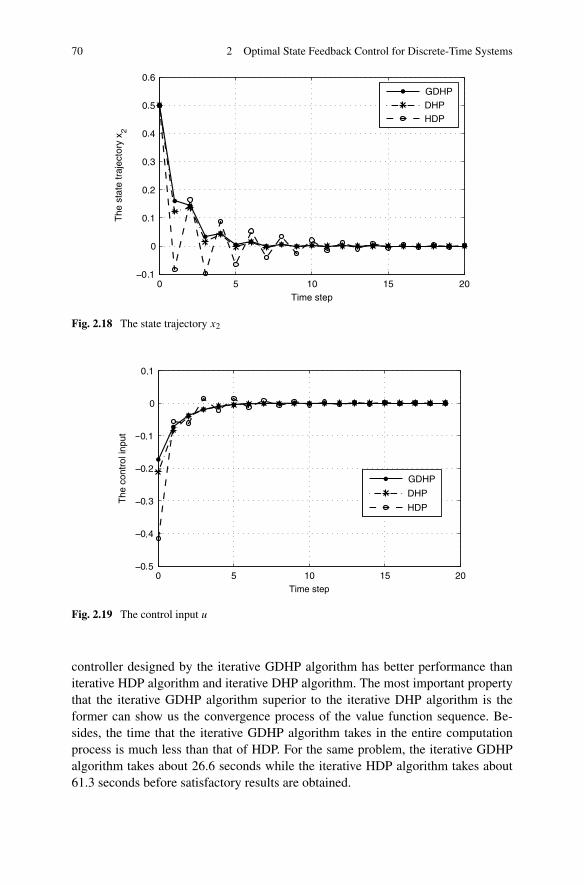
70 2 Optimal State Feedback Control for Discrete-Time Systems
Fig. 2.18 The state trajectory x2
Fig. 2.19 The control input u
controller designed by the iterative GDHP algorithm has better performance thaniterative HDP algorithm and iterative DHP algorithm. The most important propertythat the iterative GDHP algorithm superior to the iterative DHP algorithm is theformer can show us the convergence process of the value function sequence. Be-sides, the time that the iterative GDHP algorithm takes in the entire computationprocess is much less than that of HDP. For the same problem, the iterative GDHPalgorithm takes about 26.6 seconds while the iterative HDP algorithm takes about61.3 seconds before satisfactory results are obtained.
2.4 Infinite-Horizon Optimal State Feedback Control Based on GHJB Algorithm 71
2.4 Infinite-Horizon Optimal State Feedback Control Basedon GHJB Algorithm
2.4.1 Problem Formulation
Consider an affine nonlinear discrete-time system of the form
x(k + 1)= f (x(k))+ g(x(k))u(k), (2.134)
where x(k) ∈ Ω ∈ Rn, f : Rn → R
n, g : Rn → Rn×m. The input satisfies u(k) ∈
Ωu, Ωu = {u(k) = [u1(k), u2(k), . . . , um(k)]T ∈ Rm : |ui(k)| < ui(k), i = 1,2,
. . . ,m}, where ui (k) is the saturating bound of the ith actuator. Let U = diag{u1, u2,
. . . , um}. Assuming that f +gu is continuous on a set Ω ⊆ Rn containing the origin,
and system (2.134) is controllable in the sense that there exists a continuous con-trol on Ω that asymptotically stabilizes the system. In this subsection, the infinite-horizon optimal control problem for nonlinear discrete-time systems with actuatorsaturation is investigated. It is desired to find the constrained state feedback inputu(x(k)) which minimizes a generalized cost functional as follows:
J (x(0), u)=∞∑
k=0
Q(x(k))+W(u(x(k))), (2.135)
where Q(x(k)) and W(u(x(k))) are positive definite on Ω . For optimal controlproblem, it is worthy to note that u(x(k)) must both stabilize the system and makethe cost functional finite, i.e., it must be an admissible control.
For system (2.134), the nonlinear discrete-time GHJB equation without consid-ering saturation is given as follows:
∇V T(x)(f (x)+ g(x)u(x)− x)+Q(x)+W(u(x))= 0, (2.136)
V (x)|x=0 = 0. (2.137)
For a given admissible control u, there exists a positive definite continuouslydifferentiable value function V (x) whose initial value V (x(0)) equals J (x(0), u).
For unconstrained control problem, a common choice of function W(u(x)) isuT(x)Ru(x), where R ∈ R
m×m is positive definite. On substitution of the optimalcontrol u∗(x) = −R−1gT(x)∇J ∗(x)/2, where J ∗(x) is the optimal value functioncorresponding to optimal control u∗(x), the GHJB equation (2.136) with the bound-ary condition (2.137) becomes the well-known HJB equation as follows:
∇J ∗T(x)(f (x)+ g(x)u(x)− x)+Q(x)
+ 1
4∇J ∗T(x)g(x)R−1gT(x)∇J ∗(x)= 0, (2.138)
J ∗(x)|x=0 = 0. (2.139)
72 2 Optimal State Feedback Control for Discrete-Time Systems
However, the HJB equation above is not suitable for constrained optimal controlproblem. To guarantee bounded controls, we introduce a generalized nonquadraticfunctional as follows:
W(u(x))= 2∫ u(x)
0Φ−T(U−1s)URds, (2.140)
where W(u(x)) is a scalar, Φ(v)= [ϕ(v1), . . . , ϕ(vm)]T and
Φ−1(u)= [ϕ(u1)−1, . . . , ϕ(um)
−1]T
are bounded one-to-one functions that belong to Cp(p) ≥ 1 and L2(Ω), satisfy-ing |ϕ(·)| ≤ 1. Moreover, ϕ(·) is a monotonic odd function with its first derivativebounded by a constant M . It is not difficult to find such functions, such as the hyper-bolic tangent function ϕ(·)= tanh(·). R is positive definite and assumed to be sym-metric for simplicity of analysis. Substituting (2.140) into (2.136), the constraineddiscrete-time GHJB equation with boundary condition is derived as follows:
∇V T(x)(f (x)+ g(x)u(x)− x)+Q(x)+ 2∫ u(x)
0Φ−T(U−1s)URds = 0,
(2.141)
V (x)|x=0 = 0. (2.142)
According to the first-order necessary condition of the optimal control, the con-strained optimal state feedback control law can be obtained as follows:
u∗(x)= UΦ
(−1
2(UR)−1gT(x)∇J ∗(x)
). (2.143)
Substitute (2.143) into (2.141), and the constrained discrete-time HJB equationcan be derived as follows:
∇J ∗T(x)
(f (x)+ gUΦ
(−1
2(UR)−1gT∇J ∗(x)
)− x
)
+Q(x)+ 2∫ UΦ(− 1
2 (UR)−1gT(x)∇J ∗(x))
0Φ−T(U−1s)URds = 0,
J ∗(x)|x=0 = 0. (2.144)
If this HJB equation can be solved for the optimal value function J ∗(x), then(2.143) gives the optimal constrained control. However, this equation is generallyimpossible to solve.
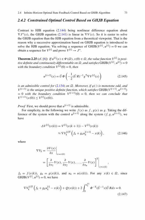
2.4 Infinite-Horizon Optimal State Feedback Control Based on GHJB Algorithm 73
2.4.2 Constrained Optimal Control Based on GHJB Equation
Contrast to HJB equation (2.144) being nonlinear difference equation about∇J ∗(x), the GHJB equation (2.141) is linear in ∇V (x). So it is easier to solvethe GHJB equation than the HJB equation from a theoretical viewpoint. That is thereason why a successive approximation based on GHJB equation is introduced tosolve the HJB equation. Via solving a sequence of GHJB(V [i], u[i]) = 0 we canobtain a sequence for V [i] and prove V [i] → J ∗.
Theorem 2.25 (cf. [6]) If u[i](x) ∈ Ψ (Ω), x(0) ∈Ω , the value function V [i] is posi-tive definite and continuously differentiable onΩ , and satisfies GHJB(V [i], u[i])= 0with the boundary condition V [i](0)= 0, then
u[i+1](x)= UΦ
(−1
2(UR)−1gT∇V [i](x)
)(2.145)
is an admissible control for (2.134) on Ω . Moreover, if ϕ(·) is monotone odd, andV [i+1] is the unique positive definite function, which satisfies GHJB(V [i+1], u[i+1])= 0 with the boundary condition V [i+1](0) = 0, then we can conclude thatV (i+1)(x(0))≤ V [i](x(0)).
Proof First, we should prove that u[i+1] is admissible.For simplicity, in the following we write f (x) as f , g(x) as g. Taking the dif-
ference of the system with the control u[i+1] along the system (f, g,u[i+1]), wehave
ΔV [i](x(k))= V [i](x(k + 1))− V [i](x(k))
≈ ∇V [i]Tk
(fk + gku
[i+1]k − x(k)
), (2.146)
where
∇Vk = ∂V (x)
∂x
∣∣∣∣x=x(k)
=[
∂
∂x1V (x),
∂
∂x2V (x), . . . ,
∂
∂xnV (x)
]T∣∣∣∣∣x=x(k)
,
fk = f (x(k)), gk = g(x(k)), and uk = u(x(k)). For any x(k) ∈ Ω , sinceGHJB(V [i], u[i])= 0, we have
∇V [i]Tk
(fk + gku
[i]k − x(k)
)+Q(x(k))+ 2
∫ u[i]k
0Φ−T(U−1s)URds = 0.
(2.147)
74 2 Optimal State Feedback Control for Discrete-Time Systems
Substituting (2.147) into (2.146), we have
ΔV [i](x(k))= ∇V [i]Tk gk
(u
[i+1]k − u
[i]k
)−Q(x(k))
− 2∫ u
[i]k
0Φ−T(U−1s)URds. (2.148)
Since
∇V [i]Tk (x)gk = −2Φ−T
(U−1u
[i+1]k
)UR, (2.149)
we get
ΔV [i](x(k))= −Q(x(k))+ 2
[Φ−T
(U−1u
[i+1]k
)UR
(u
[i]k − u
[i+1]k
)
−∫ u
[i]k
0Φ−T(U−1s)URds
]. (2.150)
Because ϕ and ϕ−1 are monotone odd, the second term of (2.150) is negative. Thisimplies that ΔV [i](x(k)) < 0 for x(k) �= 0. Thus, V [i] is a Lyapunov function foru[i+1] on Ω and the system (2.134) is asymptotically stable.
Next, we are ready to show that the value function of the system with the updatedcontrol u[i+1] is finite.
Since u[i] is admissible, from Definition 2.1, we get
V [i](x(0))= J (x(0), u[i]) <∞, x(0) ∈Ω. (2.151)
The value function for u[i+1] is
V (x(0), u[i+1])=∞∑
k=0
{Q(x(k)+ 2
∫ u[i+1]k
0Φ−T(U−1s)URds
}, (2.152)
where x(k) is the state trajectory of system with admissible control u[i+1].From (2.150) and (2.152), we have
V [i](x(∞))−V [i](x(0))
=∞∑
k=0
ΔV [i](k)
=∞∑
k=0
{−Q(x(k))+ 2[Φ−T(U−1u
[i+1]k )UR(u
[i]k − u
[i+1]k )
−∫ u
[i]k
0Φ−1(U−1s)URds]
}
2.4 Infinite-Horizon Optimal State Feedback Control Based on GHJB Algorithm 75
= − J (x(0), u[i+1])+ 2∞∑
k=0
{Φ−T(U−1u
[i+1]k )UR(u
[i]k − u
[i+1]k )
+∫ u
[i+1]k
u[i]k
Φ−T(U−1s)URds
}. (2.153)
Since x(∞) = 0 and V [i](x)|x=0 = 0, we get V [i](x(∞)) = 0. By rewriting(2.152), we have
J (x(0), u[i+1])= V [i](x(0))+ 2∞∑
k=0
{Φ−T(U−1u
[i+1]k UR(u
[i]k − u
[i+1]k )
+∫ u
[i+1]k
u[i]k
Φ−T(U−1s)URds
}. (2.154)
Since ϕ and ϕ−1 are monotone odd, and the second term of (2.154) is less than0, we have
J (x(0), u[i+1]) < V [i](x(0))= J (x(0), u[i]) <∞. (2.155)
Because V [i] is continuously differentiable, and g : Rn → Rn×m is a Lipschitzcontinuous function, u[i+1] is continuous. Since V [i] is positive definite and attainsits minimum at the origin, and ΔV [i] must approach 0 at the origin, from (2.145)we have u[i+1](x)|x=0 = 0.
From Definition 2.1, we know that u[i+1] is an admissible control on Ω . Sinceu[i+1] is admissible, there exists a V [i+1] satisfying GHJB(V [i+1], u[i+1])= 0, and
V [i+1](x(0))= J (x(0), u[i+1]). (2.156)
From (2.154) and (2.156), we get
V [i+1](x(0))− V [i](x(0))= −2∞∑
k=0
{Φ−T(U−1u
[i+1]k )UR(u
[i]k − u
[i+1]k )
+∫ u
[i+1]k
u[i]k
Φ−T(U−1s)URds
}
≤ 0. (2.157)
The proof is completed. �
Corollary 2.26 Given u[0](x) ∈ Ψ (Ω), if one iteratively solve the GHJB equationGHJB (V [i], u[i]) = 0 and for i = 0,1,2, . . . , update the control as u[i+1](x) =UΦ(− 1
2 (UR)−1gT∇V [i](x)), then it can be concluded that V [i](x)→ J ∗(x).
76 2 Optimal State Feedback Control for Discrete-Time Systems
Proof According to Theorem 2.25, V [i] is a decreasing sequence with a lowerbound. Since V [i] > 0 , V [i+1] − V [i] < 0 , V [i] will converge to a positive defi-nite function V [i+1] = V [i] = V d when i → ∞. Due to the HJB equation having aunique solution, we just need to prove V d = J ∗. When V [i] = V [i+1] = V d , from(2.145) we have
u[i](x)= u[i+1](x)= UΦ
(−1
2(UR)−1gTΔV [i](x)
). (2.158)
The GHJB equation with input u[i] can be written as
∇V [i](x)T(f (x)+ gUΦ
(−1
2(UR)−1gT∇V [i](x)
)− x
)+Q(x)
+ 2∫ UΦ(− 1
2 (UR)−1gT∇V [i](x))
0Φ−T(U−1s)URds = 0, (2.159)
V [i](x)|x=0 = 0. (2.160)
From (2.144), the conclusion can be drawn that (2.159) with boundary condition(2.160) is the HJB equation. This implies that V [i](x)→ J ∗(x), u[i](x)→ u∗(x). �
In the next part, we are ready to discuss how to design the nearly optimal satu-rated controller using NNs. In general, the closed-form solution of GHJB equation(2.141) cannot be obtained even though solving GHJB equation (2.141) is easierthan solving HJB equation (2.144). In this section, a neural network is used to ap-proximate the solution V (x) of constrained nonlinear discrete-time GHJB equation.Finally, the nearly optimal state feedback control is obtained according to (2.143).
V (x) is approximated by a neural network as follows:
VL(x)=L∑
j=1
wjσj (x)=WTLσL(x), (2.161)
where wj are the weights of the neural network, σj (x) are the activation func-tions, σj (x) are continuous and satisfy σj (x)|x=0 = 0. L is the number of hidden-layer neurons. σL(x)≡ [σ1(x), σ2(x), . . . , σL(x)]T is the vector activation function,WL(x)≡ [w1(x),w2(x), . . . ,wL(x)]T is the vector weight. The control objective isto make the residual error minimum in a least-square sense by tuning the weights.
Substituting (2.161) into (2.141), we have
GHJB
⎛
⎝VL =L∑
j=1
wjσj ,u
⎞
⎠= eL(x). (2.162)
2.4 Infinite-Horizon Optimal State Feedback Control Based on GHJB Algorithm 77
The method of weighted residuals is used to find the least-square solution, i.e.,⟨∂(eL(x))
∂WL(x), eL(x)
⟩= 0, (2.163)
where 〈f,g〉 = ∫Ωfgdx is a Lebesgue integral.
By expanding (2.163), we get
〈∇σL(x)Δx,∇σL(x)Δx〉 ·WL
+⟨Q(x)+ 2
∫ u(x)
0Φ−T(U−1s)URds,∇σL(x)Δx
⟩= 0. (2.164)
Lemma 2.27 If the set {σj (x)}L1 is linearly independent and u ∈ Ωu, then the set{∇σT
j Δx}L1 is also linearly independent.
From Lemma 2.27, 〈∇σL(x)Δx,∇σL(x)Δx〉 is invertible. Therefore there existsa unique solution as follows:
WL = −〈∇σL(x)Δx,∇σL(x)Δx〉−1
×⟨Q(x)+ 2
∫ u(x)
0Φ−T(U−1s)URds,∇σL(x)Δx
⟩, (2.165)
and the control can be derived as
u= UΦ(
− 1
2(UR)−1gT∇σT
LWL
). (2.166)
For reducing computation, the integration in (2.165) is approximated by the def-inition of Riemann integration [4].
A mesh of points over the integral region can be introduced on Ω , with the sizeδx chosen as small as possible. Moreover, p is required to be larger than L, andthe activation functions are linearly independent to guarantee (ATA) invertible. Thespecific expressions are given as follows:
A= [∇σL(x)Δx|x=x1, . . . , ∇σL(x)Δx|x=xp ]T, (2.167)
B =
⎡
⎢⎢⎢⎣
Q(x)+ 2∫ u(x)
0 Φ−T(U−1s)URds
∣∣∣x=x1
...
Q(x)+ 2∫ u(x)
0 Φ−T(U−1s)URds
∣∣∣x=xp
⎤
⎥⎥⎥⎦ , (2.168)
〈∇σL(x)Δx,∇σL(x)Δx〉 = lim‖δx‖→0(ATA) · δx, (2.169)
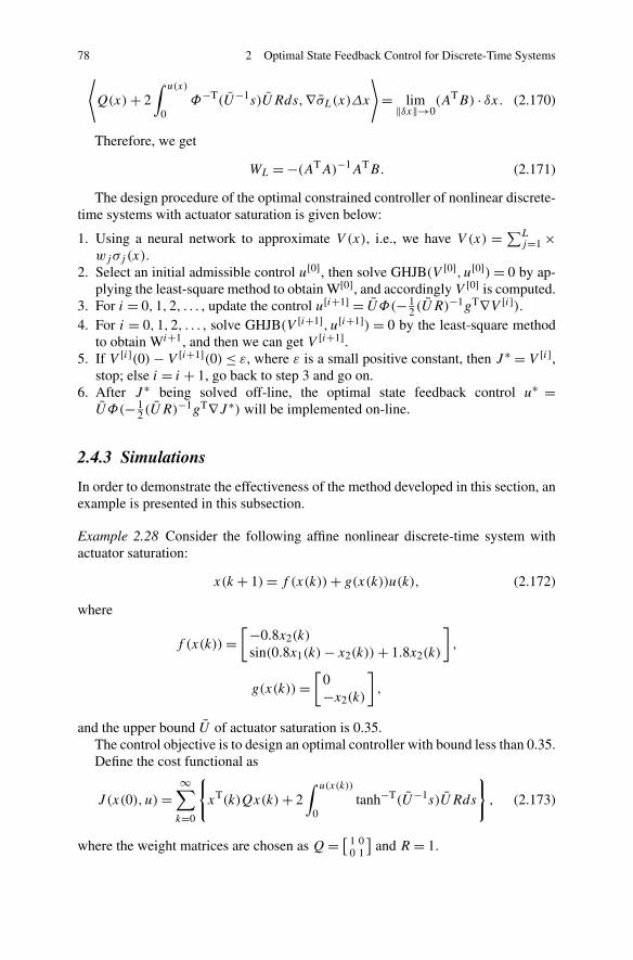
78 2 Optimal State Feedback Control for Discrete-Time Systems
⟨Q(x)+ 2
∫ u(x)
0Φ−T(U−1s)URds,∇σL(x)Δx
⟩= lim‖δx‖→0
(ATB) · δx. (2.170)
Therefore, we get
WL = −(ATA)−1ATB. (2.171)
The design procedure of the optimal constrained controller of nonlinear discrete-time systems with actuator saturation is given below:
1. Using a neural network to approximate V (x), i.e., we have V (x) = ∑Lj=1 ×
wjσj (x).2. Select an initial admissible control u[0], then solve GHJB(V [0], u[0])= 0 by ap-
plying the least-square method to obtain W[0], and accordingly V [0] is computed.3. For i = 0,1,2, . . . , update the control u[i+1] = UΦ(− 1
2 (UR)−1gT∇V [i]).
4. For i = 0,1,2, . . . , solve GHJB(V [i+1], u[i+1]) = 0 by the least-square methodto obtain Wi+1, and then we can get V [i+1].
5. If V [i](0)− V [i+1](0)≤ ε, where ε is a small positive constant, then J ∗ = V [i],stop; else i = i + 1, go back to step 3 and go on.
6. After J ∗ being solved off-line, the optimal state feedback control u∗ =UΦ(− 1
2 (UR)−1gT∇J ∗) will be implemented on-line.
2.4.3 Simulations
In order to demonstrate the effectiveness of the method developed in this section, anexample is presented in this subsection.
Example 2.28 Consider the following affine nonlinear discrete-time system withactuator saturation:
x(k + 1)= f (x(k))+ g(x(k))u(k), (2.172)
where
f (x(k))=[−0.8x2(k)
sin(0.8x1(k)− x2(k))+ 1.8x2(k)
],
g(x(k))=[
0−x2(k)
],
and the upper bound U of actuator saturation is 0.35.The control objective is to design an optimal controller with bound less than 0.35.Define the cost functional as
J (x(0), u)=∞∑
k=0
{xT(k)Qx(k)+ 2
∫ u(x(k))
0tanh−T(U−1s)URds
}, (2.173)
where the weight matrices are chosen as Q= [ 1 00 1
]and R = 1.
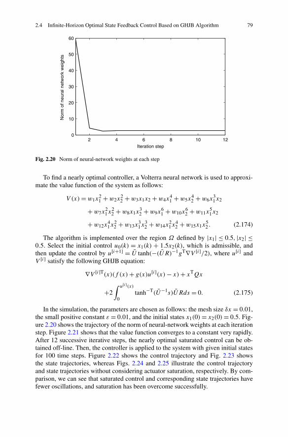
2.4 Infinite-Horizon Optimal State Feedback Control Based on GHJB Algorithm 79
Fig. 2.20 Norm of neural-network weights at each step
To find a nearly optimal controller, a Volterra neural network is used to approxi-mate the value function of the system as follows:
V (x)=w1x21 +w2x
22 +w3x1x2 +w4x
41 +w5x
42 +w6x
31x2
+w7x21x
22 +w8x1x
32 +w9x
61 +w10x
62 +w11x
51x2
+w12x41x
22 +w13x
31x
32 +w14x
21x
42 +w15x1x
52 . (2.174)
The algorithm is implemented over the region Ω defined by |x1| ≤ 0.5, |x2| ≤0.5. Select the initial control u0(k) = x1(k) + 1.5x2(k), which is admissible, andthen update the control by u[i+1] = U tanh(−(UR)−1gT∇V [i]/2), where u[i] andV [i] satisfy the following GHJB equation:
∇V [i]T(x)(f (x)+ g(x)u[i](x)− x)+ xTQx
+2∫ u[i](x)
0tanh−T(U−1s)URds = 0. (2.175)
In the simulation, the parameters are chosen as follows: the mesh size δx = 0.01,the small positive constant ε = 0.01, and the initial states x1(0)= x2(0)= 0.5. Fig-ure 2.20 shows the trajectory of the norm of neural-network weights at each iterationstep. Figure 2.21 shows that the value function converges to a constant very rapidly.After 12 successive iterative steps, the nearly optimal saturated control can be ob-tained off-line. Then, the controller is applied to the system with given initial statesfor 100 time steps. Figure 2.22 shows the control trajectory and Fig. 2.23 showsthe state trajectories, whereas Figs. 2.24 and 2.25 illustrate the control trajectoryand state trajectories without considering actuator saturation, respectively. By com-parison, we can see that saturated control and corresponding state trajectories havefewer oscillations, and saturation has been overcome successfully.
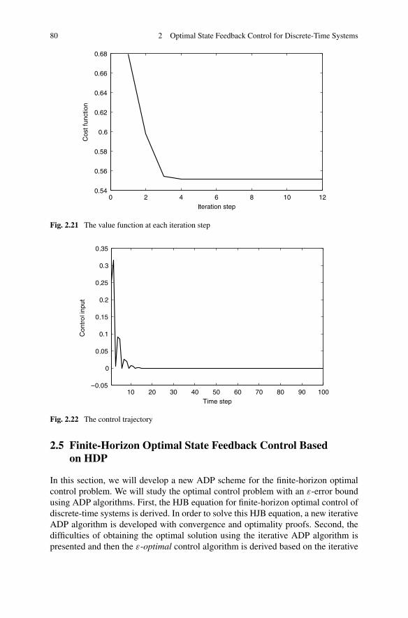
80 2 Optimal State Feedback Control for Discrete-Time Systems
Fig. 2.21 The value function at each iteration step
Fig. 2.22 The control trajectory
2.5 Finite-Horizon Optimal State Feedback Control Basedon HDP
In this section, we will develop a new ADP scheme for the finite-horizon optimalcontrol problem. We will study the optimal control problem with an ε-error boundusing ADP algorithms. First, the HJB equation for finite-horizon optimal control ofdiscrete-time systems is derived. In order to solve this HJB equation, a new iterativeADP algorithm is developed with convergence and optimality proofs. Second, thedifficulties of obtaining the optimal solution using the iterative ADP algorithm ispresented and then the ε-optimal control algorithm is derived based on the iterative
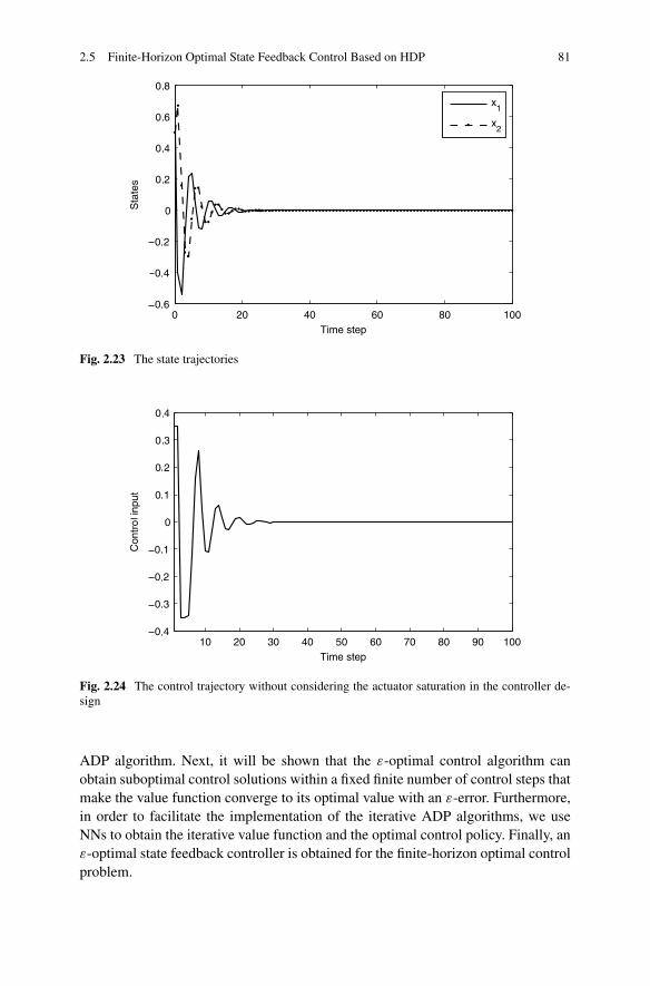
2.5 Finite-Horizon Optimal State Feedback Control Based on HDP 81
Fig. 2.23 The state trajectories
Fig. 2.24 The control trajectory without considering the actuator saturation in the controller de-sign
ADP algorithm. Next, it will be shown that the ε-optimal control algorithm canobtain suboptimal control solutions within a fixed finite number of control steps thatmake the value function converge to its optimal value with an ε-error. Furthermore,in order to facilitate the implementation of the iterative ADP algorithms, we useNNs to obtain the iterative value function and the optimal control policy. Finally, anε-optimal state feedback controller is obtained for the finite-horizon optimal controlproblem.
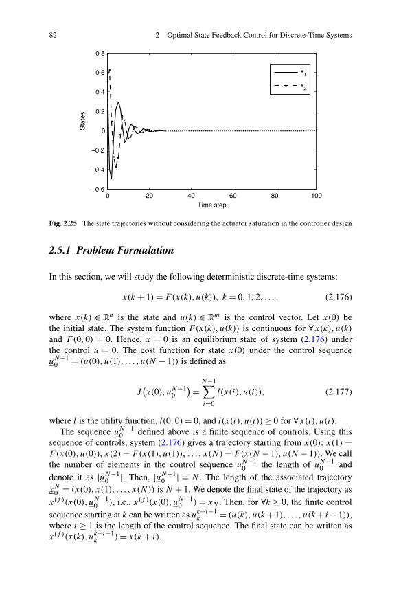
82 2 Optimal State Feedback Control for Discrete-Time Systems
Fig. 2.25 The state trajectories without considering the actuator saturation in the controller design
2.5.1 Problem Formulation
In this section, we will study the following deterministic discrete-time systems:
x(k + 1)= F(x(k), u(k)), k = 0,1,2, . . . , (2.176)
where x(k) ∈ Rn is the state and u(k) ∈ R
m is the control vector. Let x(0) bethe initial state. The system function F(x(k), u(k)) is continuous for ∀x(k), u(k)and F(0,0) = 0. Hence, x = 0 is an equilibrium state of system (2.176) underthe control u = 0. The cost function for state x(0) under the control sequenceuN−1
0 = (u(0), u(1), . . . , u(N − 1)) is defined as
J(x(0), uN−1
0
)=N−1∑
i=0
l(x(i), u(i)), (2.177)
where l is the utility function, l(0,0)= 0, and l(x(i), u(i))≥ 0 for ∀x(i), u(i).The sequence uN−1
0 defined above is a finite sequence of controls. Using thissequence of controls, system (2.176) gives a trajectory starting from x(0): x(1) =F(x(0), u(0)), x(2)= F(x(1), u(1)), . . . , x(N)= F(x(N − 1), u(N − 1)). We callthe number of elements in the control sequence uN−1
0 the length of uN−10 and
denote it as |uN−10 |. Then, |uN−1
0 | = N . The length of the associated trajectoryxN0 = (x(0), x(1), . . . , x(N)) is N + 1. We denote the final state of the trajectory asx(f )(x(0), uN−1
0 ), i.e., x(f )(x(0), uN−10 ) = xN . Then, for ∀k ≥ 0, the finite control
sequence starting at k can be written as uk+i−1k = (u(k), u(k+1), . . . , u(k+ i−1)),
where i ≥ 1 is the length of the control sequence. The final state can be written asx(f )(x(k), uk+i−1
k )= x(k + i).
2.5 Finite-Horizon Optimal State Feedback Control Based on HDP 83
We note that the cost function defined in (2.177) does not have the term as-sociated with the final state since in the present study we specify the final statex(N) = F(x(N − 1), u(N − 1)) to be at the origin, i.e., x(N) = x(f ) = 0. Forthe present finite-horizon optimal control problem, the feedback controller u(k) =u(x(k)) must not only drive the system state to zero within a finite number oftime steps but also guarantee the cost function (2.177) to be finite, i.e., uN−1
k =(u(x(k)), u(x(k + 1)), . . . , u(x(N − 1))) must be a finite-horizon admissible con-trol sequence, where N > k is a finite integer.
Definition 2.29 A control sequence uN−1k is said to be finite-horizon admissible for
a state x(k) ∈Rn, if x(f )(x(k), uN−1
k )= 0 and J (x(k), uN−1k ) is finite, where N > k
is a finite integer.
A state x(k) is said to be finite-horizon controllable (controllable for brief) ifthere is a finite-horizon admissible control sequence associated with this state.
Let uk be an arbitrary finite-horizon admissible control sequence starting at k andlet
Ax(k) = {uk : x(f )(x(k), uk
)= 0}
be the set of all finite-horizon admissible control sequences of x(k). Let
A(i)x(k) = {
uk+i−1k : x(f )(x(k), uk+i−1
k
)= 0,∣∣uk+i−1
k
∣∣= i}
be the set of all finite-horizon admissible control sequences of x(k) with length i.Then, Ax(k) = ⋃
1≤i<∞ A(i)x(k). In this notation, a state x(k) is controllable if and
only if Ax(k) �= ∅.For any given system state x(k), the objective of the present finite-horizon
optimal control problem is to find a finite-horizon admissible control sequenceuN−1k ∈ A
(N−k)x(k) ⊆ Ax(k) to minimize the cost J (x(k), uN−1
k ). The control sequence
uN−1k has finite length. However, before it is determined, we do not know its length
which means that the length of the control sequence |uN−1k | =N − k is unspecified.
This kind of optimal control problems have been called finite-horizon problemswith unspecified terminal time [3] (but in the present case, with fixed terminal statex(f ) = 0).
Define the optimal value function as
J ∗(x(k))= infuk
{J (x(k), uk) : uk ∈Ax(k)
}. (2.178)
Then, according to Bellman’s principle of optimality, J ∗(x(k)) satisfies the discrete-time HJB equation
J ∗(x(k))= minuk
{l(x(k), u(k))+ J ∗(F (x(k), u(k)))
}. (2.179)
84 2 Optimal State Feedback Control for Discrete-Time Systems
Now, define the law of optimal control sequence starting at k by
u∗(x(k))= arg infuk
{J (x(k), uk) : uk ∈ Ax(k)
},
and define the law of optimal control vector by
u∗(x(k))= arg minu(k)
{l(x(k), u(k))+ J ∗(F (x(k), u(k)))
}.
In other words, u∗(x(k))= u∗k and u∗(x(k))= u∗
k . Hence, we have
J ∗(x(k))= l(x(k), u∗k)+ J ∗(F (x(k), u∗
k)).
2.5.2 Finite-Horizon Optimal State Feedback Control Basedon HDP
In this subsection, a new iterative ADP algorithm is developed to obtain the finite-horizon optimal controller for nonlinear systems. The goal of the present iterativeADP algorithm is to construct an optimal control policy u∗(x(k)), k = 0,1, . . . ,which drives the system from an arbitrary initial state x(0) to the singularity 0 withina finite time, and simultaneously minimizes the performance index function. Con-vergence proofs will also be given to show that the performance index function willindeed converge to the optimum.
2.5.2.1 Derivation and Properties of the Iterative ADP Algorithm
We first consider the case where for any state x(k), there exists a control vector u(k)such that F(x(k), u(k))= 0, i.e., we can control the state of system (2.176) to zeroin one step from any initial state. For the case where F(x(k), u(k)) = 0 does nothold, we will discuss and solve the problem later in the subsection.
In the iterative ADP algorithm, the value function and control policy are updatedby recursive iterations, with the iteration index number i increasing from 0 and withthe initial performance index function V0(x)= 0 for ∀x ∈ R
n.The value function for i = 1 is computed as
V1(x(k))=minu(k)
{l(x(k), u(k))+ V0(F (x(k), u(k)))}subject to F(x(k), u(k))= 0
=minu(k)
l(x(k), u(k)) subject to F(x(k), u(k))= 0
= l(x(k), u∗k(x(k))), (2.180)
2.5 Finite-Horizon Optimal State Feedback Control Based on HDP 85
where V0(F (x(k), u(k))) = 0 and F(x(k), u∗k(x(k))) = 0. The control vector
v1(x(k)) for i = 1 is chosen as v1(x(k)) = u∗k(x(k)). Therefore, (2.180) can also
be written as
V1(x(k))=minu(k)
l(x(k), u(k)) subject to F(x(k), u(k))= 0
= l(x(k), v1(x(k))), (2.181)
where
v1(x(k))= arg minu(k)
l(x(k), u(k)) subject to F(x(k), u(k))= 0. (2.182)
For i = 2,3,4, . . . , the iterative ADP algorithm will be implemented as follows:
Vi(x(k))= minu(k)
{l(x(k), u(k))+ Vi−1(F (x(k), u(k)))}
= l(x(k), vi(x(k)))+ Vi−1(F (x(k), vi(x(k)))), (2.183)
where
vi(x(k))= arg minu(k)
{l(x(k), u(k))+ Vi−1(x(k + 1))}
= arg minu(k)
{l(x(k), u(k))+ Vi−1(F (x(k), u(k)))} . (2.184)
Equations (2.181)–(2.184) form the iterative ADP algorithm.
Remark 2.30 Equations (2.181)–(2.184) in the iterative ADP algorithm are similarto the HJB equation (2.179), but they are not the same. There are at least two obviousdifferences:
1. For any finite time k, if x(k) is the state at k, then the optimal value functionin HJB equation (2.179) is unique, i.e., J ∗(x(k)), while in the iterative ADPequations (2.181)–(2.184), the value function is different for each iteration indexi, i.e., Vi(x(k)) �= Vj (x(k)) for ∀ i �= j in general.
2. For any finite time k, if x(k) is the state at k, then the optimal control law ob-tained by HJB equation (2.179) possesses the unique optimal control expres-sion, i.e., u∗
k = u∗(x(k)), while the control law solved by the iterative ADP algo-rithm (2.181)–(2.184) is different from each other for each iteration index i, i.e.,vi(x(k)) �= vj (x(k)) for ∀ i �= j in general.
Remark 2.31 According to (2.177) and (2.183), we have
Vi+1(x(k))= minuk+ik
{J(x(k), uk+i
k
) : uk+ik ∈A
(i+1)x(k)
}. (2.185)
86 2 Optimal State Feedback Control for Discrete-Time Systems
Since
Vi+1(x(k))= minu(k)
{l(x(k), u(k))+ Vi(x(k + 1))}
= minu(k)
{l(x(k), u(k))+ min
u(k+1)
{l(x(k + 1), u(k + 1))
+ minu(k+2)
{l(x(k + 2), u(k + 2))+ · · ·
+ minu(k+i−1)
{l(x(k + i − 1), u(k + i − 1))
+V1(x(k + i))} · · ·}}}
,
where
V1(x(k + i))= minu(k+i)
l(x(k + i), u(k + i))
subject to F(x(k + i), u(k + i))= 0,
we obtain
Vi+1(x(k))=minuk+ik
{l(x(k), u(k))+ l(x(k + 1), u(k + 1))
+· · · + l(x(k + i), u(k + i))}subject to F(x(k + i), u(k + i))= 0,
=minuk+ik
{J(x(k), uk+i
k
) : uk+ik ∈ A
(i+1)x(k)
}.
Using the notation in (2.184), we can also write
Vi+1(x(k))=i∑
j=0
l(x(k + j), vi+1−j (x(k + j))
). (2.186)
In the above, we can see that the value function J ∗(x(k)) solved by HJB equation(2.179) is replaced by a sequence of iterative value functions Vi(x(k)) and the opti-mal control law u∗(x(k)) is replaced by a sequence of iterative control law vi(x(k)),where i ≥ 1 is the index of iteration. We can prove that J ∗(x(k)) defined in (2.178)is the limit of Vi(x(k)) as i → ∞.
Theorem 2.32 Let x(k) be an arbitrary state vector. Suppose that A(1)x(k) �= ∅. Then,
the value function Vi(x(k)) obtained by (2.181)–(2.184) is a monotonically nonin-creasing sequence for ∀ i ≥ 1, i.e., Vi+1(x(k))≤ Vi(x(k)) for ∀ i ≥ 1.
2.5 Finite-Horizon Optimal State Feedback Control Based on HDP 87
Proof We prove this by mathematical induction. First, we let i = 1. Then, we haveV1(x(k)) given as in (2.181) and the finite-horizon admissible control sequence isukk = (v1(x(k))).
Next, we show that there exists a finite-horizon admissible control sequence uk+1k
with length 2 such that J (x(k), uk+1k )= V1(x(k)). The trajectory starting from x(k)
under the control of ukk = (v1(x(k))) is x(k+1)= F(x(k), v1(x(k)))= 0. Then, wecreate a new control sequence uk+1
k by adding a 0 to the end of sequence ukk to obtainthe control sequence u
k+1k = (u
kk,0). Obviously, |uk+1
k | = 2. The state trajectoryunder the control of uk+1
k is x(k + 1) = F(x(k), v1(x(k))) = 0 and x(k + 2) =F(x(k + 1), u(k + 1)), where u(k + 1) = 0. Since x(k + 1) = 0 and F(0,0) = 0,we have x(k + 2) = 0. So, uk+1
k is a finite-horizon admissible control sequence.Furthermore,
J (x(k), uk+1k )= l(x(k), v1(x(k)))+ l(x(k + 1), u(k + 1))
= l(x(k), v1(x(k)))
=V1(x(k))
since l(x(k + 1), u(k + 1)) = l(0,0) = 0. On the other hand, according to Re-mark 2.31, we have
V2(x(k))= minuk+1k
{J(x(k), uk+1
k
) : uk+1k ∈A
(2)x(k)
}.
Then, we obtain
V2(x(k))=minuk+1k
{J(x(k), uk+1
k
) : uk+1k ∈A
(2)x(k)
}
≤ J(x(k), u
k+1k
)
= V1(x(k)). (2.187)
Therefore, the theorem holds for i = 1.Assume that the theorem holds for any i = q , where q > 1. From (2.186), we
have
Vq(x(k))=q−1∑
j=0
l(x(k + j), vq−j (x(k + j))
).
The corresponding finite-horizon admissible control sequence is uk+q−1k =
(vq(x(k)), vq−1(x(k + 1)), . . . , v1(x(k + q − 1))).For i = q + 1, we create a control sequence
uk+qk = (
vq(x(k)), vq−1(x(k + 1)), . . . , v1(x(k + q − 1)),0)
88 2 Optimal State Feedback Control for Discrete-Time Systems
with length q + 1. Then, the state trajectory under the control of uk+qk is x(k),
x(k + 1)= F(x(k), vq(x(k))), x(k + 2)= F(x(k + 1), vq−1(x(k + 1))), . . ., x(k +q) = F(x(k + q − 1), v1(x(k + q − 1))) = 0, x(k + q + 1) = F(x(k + q),0) = 0.So, uk+q
k is a finite-horizon admissible control sequence. The value function underthis control sequence is
J (x(k), uk+qk )= l(x(k), vq(x(k)))+ l(x(k + 1), vq−1(x(k + 1)))
+ · · · + l(x(k + q − 1), v1(x(k + q − 1)))+ l(x(k + q),0)
=q−1∑
j=0
l(x(k + j), vq−j (x(k + j))
)
=Vq(x(k))
since l(x(k + q),0)= l(0,0)= 0.On the other hand, we have
Vq+1(x(k))= minuk+qk
{J(x(k), u
k+qk
) : uk+qk ∈ A
(q+1)x(k)
}.
Thus, we obtain
Vq+1(x(k))= minuk+qk
{J(x(k), u
k+qk
) : uk+qk ∈ A
(q+1)x(k)
}
≤ J(x(k), u
k+qk
)
= Vq(x(k)),
which completes the proof. �
From Theorem 2.32, we know that the value function Vi(x(k))≥ 0 is a monoton-ically nonincreasing sequence and is bounded below for iteration index i = 1,2, . . . .Now, we can derive the following theorem.
Theorem 2.33 Let x(k) be an arbitrary state vector. Define the performance indexfunction V∞(x(k)) as the limit of the iterative function Vi(x(k)), i.e.,
V∞(x(k))= limi→∞Vi(x(k)). (2.188)
Then, we have
V∞(x(k))= minu(k)
{l(x(k), u(k))+ V∞(x(k + 1))}.
Proof Let ηk = η(x(k)) be any admissible control vector. According to Theorem2.32, for ∀ i, we have
V∞(x(k))≤ Vi+1(x(k))≤ l(x(k), ηk)+ Vi(x(k + 1)).
2.5 Finite-Horizon Optimal State Feedback Control Based on HDP 89
Let i → ∞, we have
V∞(x(k))≤ l(x(k), ηk)+ V∞(x(k + 1)),
which is true for ∀ηk . Therefore,
V∞(x(k))≤ minu(k)
{l(x(k), u(k))+ V∞(x(k + 1))}. (2.189)
Let ε > 0 be an arbitrary positive number. Since Vi(x(k)) is nonincreasing for i ≥ 1and limi→∞ Vi(x(k))= V∞(x(k)), there exists a positive integer p such that
Vp(x(k))− ε ≤ V∞(x(k))≤ Vp(x(k)).
From (2.183), we have
Vp(x(k))=minu(k)
{l(x(k), u(k))+ Vp−1(F (x(k), u(k)))}
= l(x(k), vp(x(k)))+ Vp−1(F (x(k), vp(x(k)))).
Hence,
V∞(x(k))≥ l(x(k), vp(x(k)))+ Vp−1(F (x(k), vp(x(k))))− ε
≥ l(x(k), vp(x(k)))+ V∞(F (x(k), vp(x(k))))− ε
≥ minu(k)
{l(x(k), u(k))+ V∞(x(k + 1))} − ε.
Since ε is arbitrary, we have
V∞(x(k))≥ minu(k)
{l(x(k), u(k))+ V∞(x(k + 1))}. (2.190)
Combining (2.189) and (2.190), we prove the theorem. �
Next, we will prove that the iterative value function Vi(x(k)) converges to theoptimal value function J ∗(x(k)) as i → ∞.
Theorem 2.34 (cf. [14]) Let V∞(x(k)) be defined in (2.188). If the system statex(k) is controllable, then we have the value function V∞(x(k)) equal to the optimalvalue function J ∗(x(k)), i.e.,
limi→∞Vi(x(k))= J ∗(x(k)),
where Vi(x(k)) is defined in (2.183).
Proof According to (2.178) and (2.185), we have
J ∗(x(k))≤ minuk+i−1k
{J (x(k), uk+i−1
k ) : uk+i−1k ∈ A
(i)x(k)
}= Vi(x(k)).
90 2 Optimal State Feedback Control for Discrete-Time Systems
Then, let i → ∞, and we obtain
J ∗(x(k))≤ V∞(x(k)). (2.191)
Next, we show that
V∞(x(k))≤ J ∗(x(k)). (2.192)
For any ω > 0, by the definition of J ∗(x(k)) in (2.178), there exists ηk∈ Ax(k) such
that
J (x(k), ηk)≤ J ∗(x(k))+ω. (2.193)
Suppose that |ηk| = p. Then, η
k∈A
(p)
x(k). So, by Theorem 2.32 and (2.185), we have
V∞(x(k)) ≤ Vp(x(k))
= minuk+p−1k
{J (x(k), u
k+p−1k ) : uk+p−1
k ∈ A(p)
x(k)
}
≤ J (x(k), ηk)
≤ J ∗(x(k))+ω.
Since ω is chosen arbitrarily, we know that (2.192) is true. Therefore, from (2.191)and (2.192), we have proven the theorem. �
We can now present the following corollary.
Corollary 2.35 Let the value function Vi(x(k)) be defined by (2.183). If the systemstate x(k) is controllable, then the iterative control law vi(x(k)) converges to theoptimal control law u∗(x(k)), i.e.,
limi→∞vi(x(k))= u∗(x(k))
Remark 2.36 Generally speaking, for the finite-horizon optimal control problem,the optimal value function depends not only on state x(k) but also on the time left(see [7] and [11]). For the finite-horizon optimal control problem with unspecifiedterminal time, we have proved that the iterative value functions converge to theoptimal as the iterative index i reaches infinity. Then, the time left is negligible andwe say that the optimal value function J ∗(x(k)) is only a function of the state x(k)which is like the case of infinite-horizon optimal control problems.
According to Theorem 2.34 and Corollary 2.35, we know that if x(k) is control-lable, then, as i → ∞, the iterative value function Vi(x(k)) converges to the optimalvalue function J ∗(x(k)) and the iterative control law vi(x(k)) also converges to theoptimal control law u∗(x(k)). So, it is important to note that for controllable state
2.5 Finite-Horizon Optimal State Feedback Control Based on HDP 91
x(k), the iterative value functions Vi(x(k)) are well defined for all i under the iter-ative control law vi(x(k)).
Let T0 = {0}. For i = 1,2, . . . , define
Ti = {x(k) ∈ Rn| ∃u(k) ∈R
m s.t. F(x(k), u(k)) ∈ Ti−1}. (2.194)
Next, we prove the following theorem.
Theorem 2.37 Let T0 = {0} and Ti be defined in (2.194). Then, for i = 0,1, . . . , wehave Ti ⊆ Ti+1.
Proof We prove the theorem by mathematical induction. First, let i = 0. Since T0 ={0} and F(0,0)= 0, we know that 0 ∈ T1. Hence, T0 ⊆ T1.
Next, assume that Ti−1 ⊆ Ti holds. Now, if x(k) ∈ Ti , we have F(x(k),
ηi−1(x(k))) ∈ Ti−1 for some ηi−1(x(k)). Hence, F(x(k), ηi−1(x(k))) ∈ Ti by theassumption of Ti−1 ⊆ Ti . So, x(k) ∈ Ti+1 by (2.194). Thus, Ti ⊆ Ti+1, which provesthe theorem. �
According to Theorem 2.37, we have
{0} = T0 ⊆ T1 ⊆ · · · ⊆ Ti−1 ⊆ Ti ⊆ · · · .We can see that by introducing the sets Ti , i = 0,1, . . . , the state x(k) can be
classified correspondingly. According to Theorem 2.37, the properties of the ADPalgorithm can be derived in the following theorem.
Theorem 2.38
(i) For any i, x(k) ∈ Ti ⇔ A(i)x(k) �= ∅ ⇔ Vi(x(k)) is defined at x(k).
(ii) Let T∞ = ⋃∞i=1 Ti . Then, x(k) ∈ T∞ ⇔ Ax(k) �= ∅ ⇔ J ∗(x(k)) is defined at
x(k) ⇔ x(k) is controllable.(iii) If Vi(x(k)) is defined at x(k), then Vj (x(k)) is defined at x(k) for every j ≥ i.(iv) J ∗(x(k)) is defined at x(k) if and only if there exists an i such that Vi(x(k)) is
defined at x(k).
2.5.2.2 The ε-Optimal Control Algorithm
In the previous subsection, we have proved that the iterative value functionVi(x(k)) converges to the optimal value function J ∗(x(k)) and J ∗(x(k)) =minuk {J (x(k), uk), u ∈Ax(k)} satisfies the Bellman’s equation (2.179) for any con-trollable state x(k) ∈ T∞.
To obtain the optimal value function J ∗(x(k)), a natural strategy is to run theiterative ADP algorithm (2.181)–(2.184) until i → ∞. But unfortunately, it is notpractical to do so. In many cases, we cannot find the equality J ∗(x(k)) = Vi(x(k))
for any finite i. That is, for any admissible control sequence uk with finite length,
92 2 Optimal State Feedback Control for Discrete-Time Systems
the cost starting from x(k) under the control of uk will be larger than, not equalto, J ∗(x(k)). On the other hand, by running the iterative ADP algorithm (2.181)–(2.184), we can obtain a control vector v∞(x(k)) and then construct a controlsequence u∞(x(k)) = (v∞(x(k)), v∞(x(k + 1)), . . . , v∞(x(k + i)), . . . ), wherex(k+ 1)= F(x(k), v∞(x(k))), . . . , x(k+ i)= F(x(k+ i − 1), v∞(x(k+ i − 1))),. . . . In general, u∞(x(k)) has infinite length. That is, the controller v∞(x(k)) can-not control the state to reach the target in finite number of steps. To overcome thisdifficulty, a new ε-optimal control method using iterative ADP algorithm will bedeveloped.
First, we will introduce our method of iterative ADP with the consideration ofthe length of control sequences. For different x(k), we will consider different lengthi for the optimal control sequence. For a given error bound ε > 0, the number i willbe chosen so that the error between J ∗(x(k)) and Vi(x(k)) is within the bound.
Let ε > 0 be any small number and x(k) ∈ T∞ be any controllable state. Let thevalue function Vi(x(k)) be defined by (2.183) and J ∗(x(k)) be the optimal valuefunction. According to Theorem 2.34, given ε > 0, there exists a finite i such that
|Vi(x(k))− J ∗(x(k))| ≤ ε. (2.195)
Definition 2.39 (cf. [14]) Let x(k) ∈ T∞ be a controllable state vector. Let ε > 0 bea small positive number. The approximate length of optimal control sequence withrespect to ε is defined as
Kε(x(k))= min{i : |Vi(x(k))− J ∗(x(k))| ≤ ε}. (2.196)
Given a small positive number ε, for any state vector x(k), the number Kε(x(k))
gives a suitable length of control sequence for optimal control starting from x(k).For x(k) ∈ T∞, since limi→∞ Vi(x(k))= J ∗(x(k)), we can always find i such that(2.195) is satisfied. Therefore, {i : |Vi(x(k))− J ∗(x(k))| ≤ ε} �= ∅ and Kε(x(k)) iswell defined.
We can see that an error ε between Vi(x(k)) and J ∗(x(k)) is introduced into theiterative ADP algorithm which makes the value function Vi(x(k)) converge withina finite number of iteration steps. In this part, we will show that the correspondingcontrol is also an effective control that drives the value function to within errorbound ε from its optimal.
From Definition 2.39, we can see that all the states x(k) that satisfy (2.196) canbe classified into one set. Motivated by the definition in (2.194), we can furtherclassify this set using the following definition.
Definition 2.40 (cf. [14]) Let ε be a positive number. Define T (ε)0 = {0} and for
i = 1,2, . . . , define
T (ε)i = {x(k) ∈ T∞ : Kε(x(k))≤ i}.
2.5 Finite-Horizon Optimal State Feedback Control Based on HDP 93
Accordingly, when x(k) ∈ T (ε)i , to find the optimal control sequence which has
value less than or equal to J ∗(x(k)) + ε, one only needs to consider the controlsequences uk with length |uk| ≤ i. The sets T (ε)
i have the following properties.
Theorem 2.41 (cf. [14]) Let ε > 0 and i = 0,1, . . . . Then:
(i) x(k) ∈ T (ε)i if and only if Vi(x(k))≤ J ∗(x(k))+ ε
(ii) T (ε)i ⊆ Ti
(iii) T (ε)i ⊆ T (ε)
i+1
(iv)⋃
i T(ε)i = T∞
(v) If ε > δ > 0, then T (ε)i ⊇ T (δ)
i
Proof (i) Let x(k) ∈ T (ε)i . By Definition 2.40, Kε(x(k)) ≤ i. Let j = Kε(x(k)).
Then, j ≤ i and by Definition 2.39, |Vj (x(k)) − J ∗(x(k))| ≤ ε. So, Vj (x(k)) ≤J ∗(x(k))+ ε. By Theorem 2.32, Vi(x(k))≤ Vj (x(k))≤ J ∗(x(k))+ ε. On the otherhand, if Vi(x(k))≤ J ∗(x(k))+ ε, then |Vi(x(k))− J ∗(x(k))| ≤ ε. So, Kε(x(k))=min{j : |Vj (x(k))− J ∗(x(k))| ≤ ε} ≤ i, which implies that x(k) ∈ T (ε)
i .
(ii) If x(k) ∈ T (ε)i , Kε(x(k)) ≤ i and |Vi(x(k)) − J ∗(x(k))| ≤ ε. So, Vi(x(k))
is defined at x(k). According to Theorem 2.38 (i), we have x(k) ∈ Ti . Hence,T (ε)i ⊆ Ti .
(iii) If x(k) ∈ T (ε)i , Kε(x(k))≤ i < i + 1. So, x(k) ∈ T (ε)
i+1. Thus, T (ε)i ⊆ T (ε)
i+1.
(iv) Obviously,⋃
i T(ε)i ⊆ T∞ since T (ε)
i are subsets of T∞. For any x(k) ∈ T∞,
let p =Kε(x(k)). Then, x(k) ∈ T (ε)p . So, x(k) ∈⋃i T
(ε)i . Hence, T∞ ⊆⋃
i T(ε)i ⊆
T∞, and we obtain,⋃
i T(ε)i = T∞.
(v) If x(k) ∈ T (δ)i , Vi(x(k)) ≤ J ∗(x(k))+ δ by part (i) of this theorem. Clearly,
Vi(x(k)) ≤ J ∗(x(k)) + ε since δ < ε. This implies that x(k) ∈ T (ε)i . Therefore,
T (ε)i ⊇ T (δ)
i . �
According to Theorem 2.41(i), T (ε)i is just the region where Vi(x(k)) is close
to J ∗(x(k)) with error less than ε. This region is a subset of Ti according to Theo-rem 2.41(ii). As stated in Theorem 2.41(iii), when i is large, the set T (ε)
i is also large.That means that, when i is large, we have a large region where we can use Vi(x(k))as the approximation of J ∗(x(k)) under certain error. On the other hand, we claimthat if x(k) is far away from the origin, we have to choose long control sequenceto approximate the optimal control sequence. Theorem 2.41(iv) means that for ev-ery controllable state x(k) ∈ T∞, we can always find a suitable control sequencewith length i to approximate the optimal control. The size of the set T (ε)
i depends
on the value of ε. Smaller value of ε gives smaller set T (ε)i which is indicated by
Theorem 2.41(v).Let x(k) ∈ T∞ be an arbitrary controllable state. If x(k) ∈ T (ε)
i , the iterativevalue function satisfies (2.195) under the control vi(x(k)), we call this control the
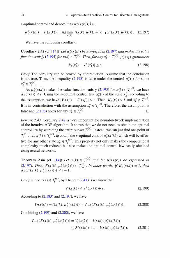
94 2 Optimal State Feedback Control for Discrete-Time Systems
ε-optimal control and denote it as μ∗ε(x(k)), i.e.,
μ∗ε(x(k))= vi(x(k))= arg min
u(k){l(x(k), u(k))+ Vi−1(F (x(k), u(k)))} . (2.197)
We have the following corollary.
Corollary 2.42 (cf. [14]) Let μ∗ε(x(k)) be expressed in (2.197) that makes the value
function satisfy (2.195) for x(k) ∈ T (ε)i . Then, for any x′
k ∈ T (ε)i , μ∗
ε(x′k) guarantees
|Vi(x′k)− J ∗(x′
k)| ≤ ε. (2.198)
Proof The corollary can be proved by contradiction. Assume that the conclusionis not true. Then, the inequality (2.198) is false under the control μ∗
ε(·) for some
x′′k ∈ T (ε)
i .
As μ∗ε(x(k)) makes the value function satisfy (2.195) for x(k) ∈ T (ε)
i , we haveKε(x(k)) ≤ i. Using the ε-optimal control law μ∗
ε(·) at the state x′′k , according to
the assumption, we have |Vi(x′′k )− J ∗(x′′
k )| > ε. Then, Kε(x′′k ) > i and x′′
k /∈ T (ε)i .
It is in contradiction with the assumption x′′k ∈ T (ε)
i . Therefore, the assumption is
false and (2.198) holds for any x′k ∈ T (ε)
i . �
Remark 2.43 Corollary 2.42 is very important for neural-network implementationof the iterative ADP algorithm. It shows that we do not need to obtain the optimalcontrol law by searching the entire subset T (ε)
i . Instead, we can just find one point of
T (ε)i , i.e., x(k) ∈ T (ε)
i , to obtain the ε-optimal control μ∗ε(x(k)) which will be effec-
tive for any other state x′k ∈ T (ε)
i . This property not only makes the computationalcomplexity much reduced but also makes the optimal control law easily obtainedusing neural networks.
Theorem 2.44 (cf. [14]) Let x(k) ∈ T (ε)i and let μ∗
ε(x(k)) be expressed in
(2.197). Then, F(x(k),μ∗ε(x(k))) ∈ T (ε)
i−1. In other words, if Kε(x(k)) = i, thenKε(F (x(k),μ
∗ε(x(k))))≤ i − 1.
Proof Since x(k) ∈ T (ε)i , by Theorem 2.41 (i) we know that
Vi(x(k))≤ J ∗(x(k))+ ε. (2.199)
According to (2.183) and (2.197), we have
Vi(x(k))= l(x(k),μ∗ε(x(k)))+ Vi−1(F (x(k),μ
∗ε(x(k)))). (2.200)
Combining (2.199) and (2.200), we have
Vi−1(F (x(k),μ∗ε(x(k))))= Vi(x(k))− l(x(k),μ∗
ε(x(k)))
≤ J ∗(x(k))+ ε − l(x(k),μ∗ε(x(k))). (2.201)
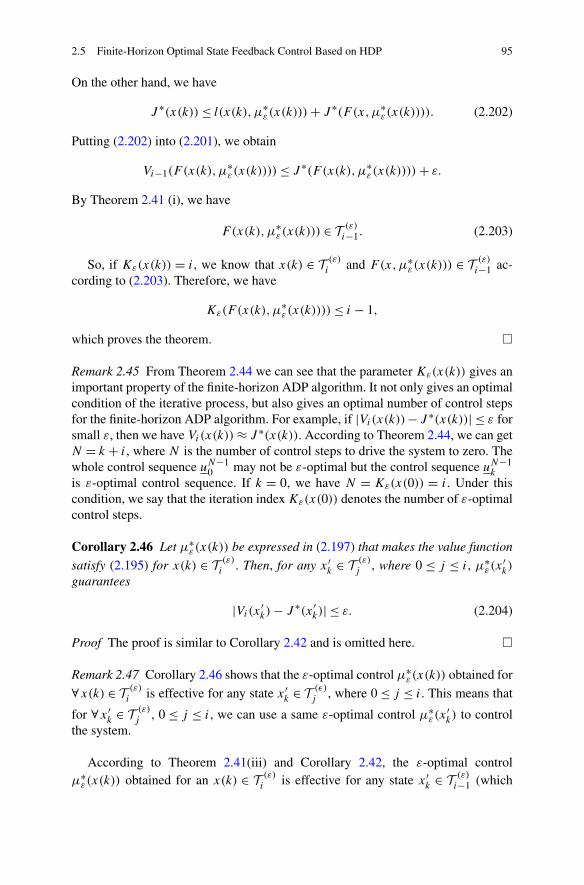
2.5 Finite-Horizon Optimal State Feedback Control Based on HDP 95
On the other hand, we have
J ∗(x(k))≤ l(x(k),μ∗ε(x(k)))+ J ∗(F (x,μ∗
ε(x(k)))). (2.202)
Putting (2.202) into (2.201), we obtain
Vi−1(F (x(k),μ∗ε(x(k))))≤ J ∗(F (x(k),μ∗
ε(x(k))))+ ε.
By Theorem 2.41 (i), we have
F(x(k),μ∗ε(x(k))) ∈ T (ε)
i−1. (2.203)
So, if Kε(x(k)) = i, we know that x(k) ∈ T (ε)i and F(x,μ∗
ε(x(k))) ∈ T (ε)i−1 ac-
cording to (2.203). Therefore, we have
Kε(F (x(k),μ∗ε(x(k))))≤ i − 1,
which proves the theorem. �
Remark 2.45 From Theorem 2.44 we can see that the parameter Kε(x(k)) gives animportant property of the finite-horizon ADP algorithm. It not only gives an optimalcondition of the iterative process, but also gives an optimal number of control stepsfor the finite-horizon ADP algorithm. For example, if |Vi(x(k))−J ∗(x(k))| ≤ ε forsmall ε, then we have Vi(x(k))≈ J ∗(x(k)). According to Theorem 2.44, we can getN = k + i, where N is the number of control steps to drive the system to zero. Thewhole control sequence uN−1
0 may not be ε-optimal but the control sequence uN−1k
is ε-optimal control sequence. If k = 0, we have N = Kε(x(0)) = i. Under thiscondition, we say that the iteration index Kε(x(0)) denotes the number of ε-optimalcontrol steps.
Corollary 2.46 Let μ∗ε(x(k)) be expressed in (2.197) that makes the value function
satisfy (2.195) for x(k) ∈ T (ε)i . Then, for any x′
k ∈ T (ε)j , where 0 ≤ j ≤ i, μ∗
ε(x′k)
guarantees
|Vi(x′k)− J ∗(x′
k)| ≤ ε. (2.204)
Proof The proof is similar to Corollary 2.42 and is omitted here. �
Remark 2.47 Corollary 2.46 shows that the ε-optimal control μ∗ε(x(k)) obtained for
∀x(k) ∈ T (ε)i is effective for any state x′
k ∈ T (ε)j , where 0 ≤ j ≤ i. This means that
for ∀x′k ∈ T (ε)
j , 0 ≤ j ≤ i, we can use a same ε-optimal control μ∗ε(x
′k) to control
the system.
According to Theorem 2.41(iii) and Corollary 2.42, the ε-optimal controlμ∗ε(x(k)) obtained for an x(k) ∈ T (ε)
i is effective for any state x′k ∈ T (ε)
i−1 (which
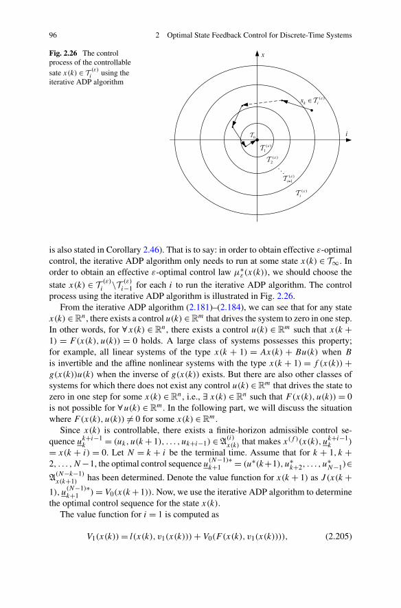
96 2 Optimal State Feedback Control for Discrete-Time Systems
Fig. 2.26 The controlprocess of the controllablesate x(k) ∈ T (ε)
i using theiterative ADP algorithm
is also stated in Corollary 2.46). That is to say: in order to obtain effective ε-optimalcontrol, the iterative ADP algorithm only needs to run at some state x(k) ∈ T∞. Inorder to obtain an effective ε-optimal control law μ∗
ε(x(k)), we should choose the
state x(k) ∈ T (ε)i \T (ε)
i−1 for each i to run the iterative ADP algorithm. The controlprocess using the iterative ADP algorithm is illustrated in Fig. 2.26.
From the iterative ADP algorithm (2.181)–(2.184), we can see that for any statex(k) ∈R
n, there exists a control u(k) ∈Rm that drives the system to zero in one step.
In other words, for ∀x(k) ∈ Rn, there exists a control u(k) ∈ R
m such that x(k +1) = F(x(k), u(k)) = 0 holds. A large class of systems possesses this property;for example, all linear systems of the type x(k + 1) = Ax(k) + Bu(k) when B
is invertible and the affine nonlinear systems with the type x(k + 1) = f (x(k)) +g(x(k))u(k) when the inverse of g(x(k)) exists. But there are also other classes ofsystems for which there does not exist any control u(k) ∈ R
m that drives the state tozero in one step for some x(k) ∈ R
n, i.e., ∃ x(k) ∈ Rn such that F(x(k), u(k)) = 0
is not possible for ∀u(k) ∈ Rm. In the following part, we will discuss the situation
where F(x(k), u(k)) �= 0 for some x(k) ∈Rm.
Since x(k) is controllable, there exists a finite-horizon admissible control se-quence uk+i−1
k = (uk, u(k+ 1), . . . , uk+i−1) ∈A(i)x(k) that makes x(f )(x(k), uk+i−1
k )
= x(k + i) = 0. Let N = k + i be the terminal time. Assume that for k + 1, k +2, . . . ,N−1, the optimal control sequence u(N−1)∗
k+1 = (u∗(k+1), u∗k+2, . . . , u
∗N−1)∈
A(N−k−1)x(k+1) has been determined. Denote the value function for x(k + 1) as J (x(k +
1), u(N−1)∗k+1 )= V0(x(k+ 1)). Now, we use the iterative ADP algorithm to determine
the optimal control sequence for the state x(k).The value function for i = 1 is computed as
V1(x(k))= l(x(k), v1(x(k)))+ V0(F (x(k), v1(x(k)))), (2.205)
2.5 Finite-Horizon Optimal State Feedback Control Based on HDP 97
where
v1(x(k))= arg minu(k)
{l(x(k), u(k))+ V0(F (x(k), u(k)))}. (2.206)
Note that the initial condition used in the above expression is the value function V0which is obtained previously for x(k + 1) and now applied at F(x(k), u(k)). Fori = 2,3,4, . . . , the iterative ADP algorithm will be implemented as follows:
Vi(x(k))= l(x(k), vi(x(k)))+ Vi−1(F (x(k), vi(x(k)))), (2.207)
where
vi(x(k))= arg minu(k)
{l(x(k), u(k))+ Vi−1(F (x(k), u(k)))} . (2.208)
Theorem 2.48 Let x(k) be an arbitrary controllable state vector. Then, the valuefunction Vi(x(k)) obtained by (2.205)–(2.208) is a monotonically nonincreasingsequence for ∀ i ≥ 0, i.e., Vi+1(x(k))≤ Vi(x(k)) for ∀ i ≥ 0.
Proof It can easily be proved by following the proof of Theorem 2.32, and the proofis omitted here. �
Theorem 2.49 Let the value function Vi(x(k)) be defined by (2.207). If the systemstate x(k) is controllable, then the value function Vi(x(k)) obtained by (2.205)–(2.208) converges to the optimal value function J ∗(x(k)) as i → ∞, i.e.,
limi→∞Vi(x(k))= J ∗(x(k)).
Proof This theorem can be proved following similar steps to the proof of Theo-rem 2.34 and the proof is omitted here. �
We can see that the iterative ADP algorithm (2.205)–(2.208) is an expansion fromof the previous one (2.181)–(2.184). So, the properties of the iterative ADP algo-rithm (2.181)–(2.184) is also effective for the current one (2.205)–(2.208). But therealso exist differences. From Theorem 2.32, we can see that Vi+1(x(k)) ≤ Vi(x(k))
for all i ≥ 1, which means that V1(x(k)) = max{Vi(x(k)) : i = 0,1, . . .}. WhileTheorem 2.48 shows that Vi+1(x(k)) ≤ Vi(x(k)) for all i ≥ 0 which means thatV0(x(k))= max{Vi(x(k)) : i = 0,1, . . .}. This difference is caused by the differenceof the initial conditions of the two iterative ADP algorithms.
In the previous iterative ADP algorithm (2.181)–(2.184), it begins with the initialvalue function V0(x(k)) = 0 since F(x(k), u(k)) = 0 can be solved. While in thecurrent iterative ADP algorithm (2.205)–(2.208), it begins with the value functionV0 for the state x(k+1) which is determined previously. This also causes the differ-ence between the proofs of Theorems 2.32 and 2.34 and the corresponding resultsin Theorems 2.48 and 2.49. But the difference of the initial conditions of the itera-tive performance index function does not affect the convergence property of the twoiterative ADP algorithms.
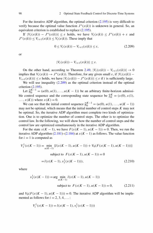
98 2 Optimal State Feedback Control for Discrete-Time Systems
For the iterative ADP algorithm, the optimal criterion (2.195) is very difficult toverify because the optimal value function J ∗(x(k)) is unknown in general. So, anequivalent criterion is established to replace (2.195).
If |Vi(x(k)) − J ∗(x(k))| ≤ ε holds, we have Vi(x(k)) ≤ J ∗(x(k)) + ε andJ ∗(x(k))≤ Vi+1(x(k))≤ Vi(x(k)). These imply that
0 ≤ Vi(x(k))− Vi+1(x(k))≤ ε, (2.209)
or
|Vi(x(k))− Vi+1(x(k))| ≤ ε.
On the other hand, according to Theorem 2.49, |Vi(x(k)) − Vi+1(x(k))| → 0implies that Vi(x(k))→ J ∗(x(k)). Therefore, for any given small ε, if |Vi(x(k))−Vi+1(x(k))| ≤ ε holds, we have |Vi(x(k))− J ∗(x(k))| ≤ ε if i is sufficiently large.
We will use inequality (2.209) as the optimal criterion instead of the optimalcriterion (2.195).
Let uK−10 = (u(0), u(1), . . . , u(K − 1)) be an arbitrary finite-horizon admissi-
ble control sequence and the corresponding state sequence be xK0 = (x(0), x(1),. . . , x(K)) where x(K)= 0.
We can see that the initial control sequence uK−10 = (u(0), u(1), . . . , u(K − 1))
may not be optimal, which means that the initial number of control steps K may notbe optimal. So, the iterative ADP algorithm must complete two kinds of optimiza-tion. One is to optimize the number of control steps. The other is to optimize thecontrol law. In the following, we will show how the number of control steps and thecontrol law are optimized simultaneously in the iterative ADP algorithm.
For the state x(K − 1), we have F(x(K − 1), u(K − 1)) = 0. Then, we run theiterative ADP algorithm (2.181)–(2.184) at x(K − 1) as follows. The value functionfor i = 1 is computed as
V 11 (x(K − 1))= min
u(K−1){l(x(K − 1), u(K − 1))+ V0(F (x(K − 1), u(K − 1)))}
subject to F(x(K − 1), u(K − 1))= 0
= l(x(K − 1), v11(x(K − 1))), (2.210)
where
v11(x(K − 1))= arg min
u(K−1)l(x(K − 1), u(K − 1))
subject to F(x(K − 1), u(K − 1))= 0, (2.211)
and V0(F (x(K − 1), u(K − 1))) = 0. The iterative ADP algorithm will be imple-mented as follows for i = 2,3,4, . . . :
V 1i (x(K − 1))= l(x(K − 1), v1
i (x(K − 1)))
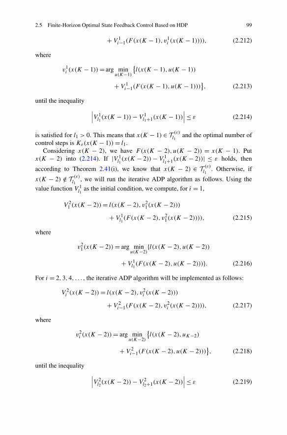
2.5 Finite-Horizon Optimal State Feedback Control Based on HDP 99
+ V 1i−1(F (x(K − 1), v1
i (x(K − 1)))), (2.212)
where
v1i (x(K − 1))= arg min
u(K−1)
{l(x(K − 1), u(K − 1))
+ V 1i−1(F (x(K − 1), u(K − 1)))
}, (2.213)
until the inequality∣∣∣V 1
l1(x(K − 1))− V 1
l1+1(x(K − 1))∣∣∣≤ ε (2.214)
is satisfied for l1 > 0. This means that x(K − 1) ∈ T (ε)l1
and the optimal number ofcontrol steps is Kε(x(K − 1))= l1.
Considering x(K − 2), we have F(x(K − 2), u(K − 2)) = x(K − 1). Putx(K − 2) into (2.214). If |V 1
l1(x(K − 2))− V 1
l1+1(x(K − 2))| ≤ ε holds, then
according to Theorem 2.41(i), we know that x(K − 2) ∈ T (ε)l1
. Otherwise, if
x(K − 2) /∈ T (ε)l1
, we will run the iterative ADP algorithm as follows. Using the
value function V 1l1
as the initial condition, we compute, for i = 1,
V 21 (x(K − 2))= l(x(K − 2), v2
1(x(K − 2)))
+ V 1l1(F (x(K − 2), v2
1(x(K − 2)))), (2.215)
where
v21(x(K − 2))= arg min
u(K−2){l(x(K − 2), u(K − 2))
+ V 1l1(F (x(K − 2), u(K − 2)))}. (2.216)
For i = 2,3,4, . . . , the iterative ADP algorithm will be implemented as follows:
V 2i (x(K − 2))= l(x(K − 2), v2
i (x(K − 2)))
+ V 2i−1(F (x(K − 2), v2
i (x(K − 2)))), (2.217)
where
v2i (x(K − 2))= arg min
u(K−2)
{l(x(K − 2), uK−2)
+ V 2i−1(F (x(K − 2), u(K − 2)))
}, (2.218)
until the inequality∣∣∣V 2
l2(x(K − 2))− V 2
l2+1(x(K − 2))∣∣∣≤ ε (2.219)
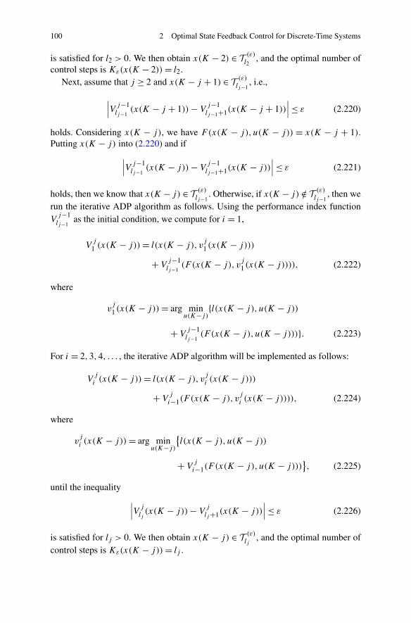
100 2 Optimal State Feedback Control for Discrete-Time Systems
is satisfied for l2 > 0. We then obtain x(K − 2) ∈ T (ε)l2
, and the optimal number ofcontrol steps is Kε(x(K − 2))= l2.
Next, assume that j ≥ 2 and x(K − j + 1) ∈ T (ε)lj−1
, i.e.,
∣∣∣V j−1lj−1
(x(K − j + 1))− Vj−1lj−1+1(x(K − j + 1))
∣∣∣≤ ε (2.220)
holds. Considering x(K − j), we have F(x(K − j), u(K − j)) = x(K − j + 1).Putting x(K − j) into (2.220) and if
∣∣∣V j−1lj−1
(x(K − j))− Vj−1lj−1+1(x(K − j))
∣∣∣≤ ε (2.221)
holds, then we know that x(K − j) ∈ T (ε)lj−1
. Otherwise, if x(K − j) /∈ T (ε)lj−1
, then werun the iterative ADP algorithm as follows. Using the performance index functionVj−1lj−1
as the initial condition, we compute for i = 1,
Vj
1 (x(K − j))= l(x(K − j), vj
1 (x(K − j)))
+ Vj−1lj−1
(F (x(K − j), vj
1 (x(K − j)))), (2.222)
where
vj
1 (x(K − j))= arg minu(K−j)
{l(x(K − j), u(K − j))
+ Vj−1lj−1
(F (x(K − j), u(K − j)))}. (2.223)
For i = 2,3,4, . . . , the iterative ADP algorithm will be implemented as follows:
Vji (x(K − j))= l(x(K − j), v
ji (x(K − j)))
+ Vj
i−1(F (x(K − j), vji (x(K − j)))), (2.224)
where
vji (x(K − j))= arg min
u(K−j)
{l(x(K − j), u(K − j))
+ Vj
i−1(F (x(K − j), u(K − j)))}, (2.225)
until the inequality∣∣∣V j
lj(x(K − j))− V
j
lj+1(x(K − j))
∣∣∣≤ ε (2.226)
is satisfied for lj > 0. We then obtain x(K − j) ∈ T (ε)lj
, and the optimal number ofcontrol steps is Kε(x(K − j))= lj .
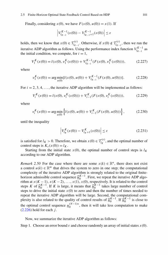
2.5 Finite-Horizon Optimal State Feedback Control Based on HDP 101
Finally, considering x(0), we have F(x(0), u(0))= x(1). If∣∣∣VK−1
lK−1(x(0))− VK−1
lK−1+1(x(0))∣∣∣≤ ε
holds, then we know that x(0) ∈ T (ε)lK−1
. Otherwise, if x(0) /∈ T (ε)lK−1
, then we run the
iterative ADP algorithm as follows. Using the performance index function VK−1lK−1
asthe initial condition, we compute, for i = 1,
VK1 (x(0))= l(x(0), vK1 (x(0)))+ VK−1
lK−1(F (x(0), vK1 (x(0)))), (2.227)
where
vK1 (x(0))= arg minu(0)
{l(x(0), u(0))+ VK−1lK−1
(F (x(0), u(0)))}. (2.228)
For i = 2,3,4, . . . , the iterative ADP algorithm will be implemented as follows:
VKi (x(0))= l(x(0), vKi (x(0)))+ VK
i−1(F (x(0), vKi (x(0)))), (2.229)
where
vKi (x(0))= arg minu(0)
{l(x(0), u(0))+ VK
i−1(F (x(0), u(0)))}, (2.230)
until the inequality∣∣∣VK
lK(x(0))− VK
lK+1(x(0))∣∣∣≤ ε (2.231)
is satisfied for lK > 0. Therefore, we obtain x(0) ∈ T (ε)lK
, and the optimal number ofcontrol steps is Kε(x(0))= lK .
Starting from the initial state x(0), the optimal number of control steps is lKaccording to our ADP algorithm.
Remark 2.50 For the case where there are some x(k) ∈ Rn, there does not exist
a control u(k) ∈ Rm that drives the system to zero in one step; the computational
complexity of the iterative ADP algorithm is strongly related to the original finite-horizon admissible control sequence uK−1
0 . First, we repeat the iterative ADP algo-rithm at x(K −1), x(K −2), . . . , x(1), x(0), respectively. It is related to the controlsteps K of uK−1
0 . If K is large, it means that uK−10 takes large number of control
steps to drive the initial state x(0) to zero and then the number of times needed torepeat the iterative ADP algorithm will be large. Second, the computational com-plexity is also related to the quality of control results of uK−1
0 . If uK−10 is close to
the optimal control sequence u(N−1)∗0 , then it will take less computation to make
(2.226) hold for each j .
Now, we summarize the iterative ADP algorithm as follows:
Step 1. Choose an error bound ε and choose randomly an array of initial states x(0).
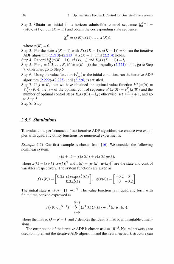
102 2 Optimal State Feedback Control for Discrete-Time Systems
Step 2. Obtain an initial finite-horizon admissible control sequence uK−10 =
(u(0), u(1), . . . , u(K − 1)) and obtain the corresponding state sequence
xK0 = (x(0), x(1), . . . , x(K)),
where x(K)= 0.Step 3. For the state x(K − 1) with F(x(K − 1), u(K − 1)) = 0, run the iterative
ADP algorithm (2.210)–(2.213) at x(K − 1) until (2.214) holds.Step 4. Record V 1
l1(x(K − 1)), v1
l1(xK−1) and Kε(x(K − 1))= l1.
Step 5. For j = 2,3, . . . ,K , if for x(K− j) the inequality (2.221) holds, go to Step7; otherwise, go to Step 6.
Step 6. Using the value function V j−1lj−1 as the initial condition, run the iterative ADP
algorithm (2.222)–(2.225) until (2.226) is satisfied.Step 7. If j = K , then we have obtained the optimal value function V ∗(x(0)) =VKlK(x(0)), the law of the optimal control sequence u∗(x(0)) = vKlK
(x(0)) and thenumber of optimal control steps Kε(x(0)) = lK ; otherwise, set j = j + 1, and goto Step 5.
Step 8. Stop.
2.5.3 Simulations
To evaluate the performance of our iterative ADP algorithm, we choose two exam-ples with quadratic utility functions for numerical experiments.
Example 2.51 Our first example is chosen from [16]. We consider the followingnonlinear system:
x(k + 1)= f (x(k))+ g(x(k))u(k),
where x(k) = [x1(k) x2(k)]T and u(k) = [u1(k) u2(k)]T are the state and controlvariables, respectively. The system functions are given as
f (x(k))=[
0.2x1(k) exp(x22(k))
0.3x32(k)
], g(x(k))=
[−0.2 00 −0.2
].
The initial state is x(0) = [1 −1]T. The value function is in quadratic form withfinite time horizon expressed as
J(x(0), uN−1
0
)=N−1∑
k=0
(xT(k)Qx(k)+ uT(k)Ru(k)
),
where the matrix Q=R = I , and I denotes the identity matrix with suitable dimen-sions.
The error bound of the iterative ADP is chosen as ε = 10−5. Neural networks areused to implement the iterative ADP algorithm and the neural-network structure can
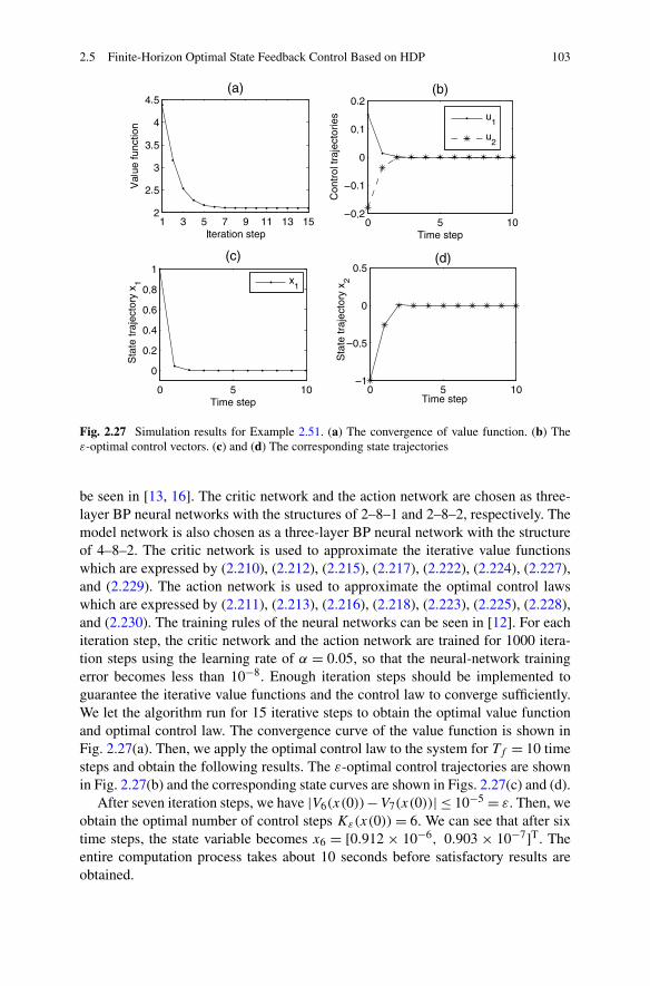
2.5 Finite-Horizon Optimal State Feedback Control Based on HDP 103
Fig. 2.27 Simulation results for Example 2.51. (a) The convergence of value function. (b) Theε-optimal control vectors. (c) and (d) The corresponding state trajectories
be seen in [13, 16]. The critic network and the action network are chosen as three-layer BP neural networks with the structures of 2–8–1 and 2–8–2, respectively. Themodel network is also chosen as a three-layer BP neural network with the structureof 4–8–2. The critic network is used to approximate the iterative value functionswhich are expressed by (2.210), (2.212), (2.215), (2.217), (2.222), (2.224), (2.227),and (2.229). The action network is used to approximate the optimal control lawswhich are expressed by (2.211), (2.213), (2.216), (2.218), (2.223), (2.225), (2.228),and (2.230). The training rules of the neural networks can be seen in [12]. For eachiteration step, the critic network and the action network are trained for 1000 itera-tion steps using the learning rate of α = 0.05, so that the neural-network trainingerror becomes less than 10−8. Enough iteration steps should be implemented toguarantee the iterative value functions and the control law to converge sufficiently.We let the algorithm run for 15 iterative steps to obtain the optimal value functionand optimal control law. The convergence curve of the value function is shown inFig. 2.27(a). Then, we apply the optimal control law to the system for Tf = 10 timesteps and obtain the following results. The ε-optimal control trajectories are shownin Fig. 2.27(b) and the corresponding state curves are shown in Figs. 2.27(c) and (d).
After seven iteration steps, we have |V6(x(0))−V7(x(0))| ≤ 10−5 = ε. Then, weobtain the optimal number of control steps Kε(x(0)) = 6. We can see that after sixtime steps, the state variable becomes x6 = [0.912 × 10⁻⁶, 0.903 × 10⁻⁷]T. Theentire computation process takes about 10 seconds before satisfactory results areobtained.
104 2 Optimal State Feedback Control for Discrete-Time Systems
Example 2.52 The second example is chosen from [9] with some modifications. Weconsider the following system:
x(k + 1)= F(x(k), u(k))= x(k)+ sin(0.1x(k)2 + u(k)), (2.232)
where x(k), u(k) ∈ R, and k = 0,1,2, . . . . The cost functional is defined as in Ex-ample 2.51 with Q = R = 1. The initial state is x(0) = 1.5. Since F(0,0) = 0,x(k) = 0 is an equilibrium state of system (2.232). But since (∂F (x(k), u(k))/
∂x(k))(0,0) = 1, system (2.232) is marginally stable at x(k) = 0 and the equilib-rium x(k)= 0 is not attractive.
We can see that, for the fixed initial state x(0), there does not exist a controlu(0) ∈ R that makes x(1) = F(x(0), u(0)) = 0. The error bound of the iterativeADP algorithm is chosen as ε = 10−4. The critic network, the action network, andthe model network are chosen as three-layer BP neural networks with the structuresof 1–3–1, 1–3–1, and 2–4–1, respectively. According to (2.232), the control can beexpressed by
u(k)= −0.1x(k)2 + sin−1(x(k + 1)− x(k))+ 2λπ, (2.233)
where λ= 0,±1,±2, . . . .To show the effectiveness of our algorithm, we choose two initial finite-horizon
admissible control sequences.Case 1. The control sequence is u
10 = (−0.225 − sin−1(0.7), −0.064 −
sin−1(0.8)) and the corresponding state sequence is x20 = (1.5,0.8,0).
For the initial finite-horizon admissible control sequences in this case, run theiterative ADP algorithm at the states x(k) = 0.8 and 1.5, respectively. For each it-erative step, the critic network and the action network are trained for 1000 iterationsteps using the learning rate of α = 0.05 so that the neural-network training ac-curacy of 10−8 is reached. After the algorithm has run for 15 iterative steps, weobtain the performance index function trajectories shown in Figs. 2.28(a) and (b),respectively. The ε-optimal control and state trajectories are shown in Figs. 2.28(c)and (d), respectively, for 10 time steps. We obtain Kε(0.8)= 5 and Kε(1.5)= 8.
Case 2. The control sequence is u30 = (−0.225 − sin−1(0.01), 2π − 2.2201 −
sin−1(0.29), −0.144 − sin−1(0.5), −sin−1(0.7)) and the corresponding state se-quence is x4
0 = (1.5,1.49,1.2,0.7,0).For the initial finite-horizon admissible control sequence in this case, run the
iterative ADP algorithm at the states x(k) = 0.7, 1.2, and 1.49, respectively. Foreach iteration step, the critic network and the action network are also trained for1000 iteration steps using the learning rate of α = 0.05, so that the neural-networktraining accuracy of 10−8 is reached. Then we obtain the value function trajectoriesshown in Figs. 2.29(a)–(c), respectively. We have Kε(0.7) = 4, Kε(1.2) = 6, andKε(1.49)= 8.
After 25 iteration steps, the value function Vi(x(k)) is sufficiently convergent atx(k)= 1.49, with V 3
8 (1.49) as the value function. For the state x(k)= 1.5, we have|V 3
8 (1.5)− V 39 (1.5)| = 0.52424 × 10⁻⁷ < ε. Therefore, the optimal value function
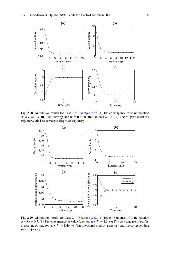
2.5 Finite-Horizon Optimal State Feedback Control Based on HDP 105
Fig. 2.28 Simulation results for Case 1 of Example 2.52. (a) The convergence of value functionat x(k) = 0.8. (b) The convergence of value function at x(k) = 1.5. (c) The ε-optimal controltrajectory. (d) The corresponding state trajectory
Fig. 2.29 Simulation results for Case 2 of Example 2.52. (a) The convergence of value functionat x(k)= 0.7. (b) The convergence of value function at x(k)= 1.2. (c) The convergence of perfor-mance index function at x(k) = 1.49. (d) The ε-optimal control trajectory and the correspondingstate trajectory
106 2 Optimal State Feedback Control for Discrete-Time Systems
at x(k)= 1.5 is V 38 (1.5) and, thus, we have x(k)= 1.5 ∈ T (ε)
8 and Kε(1.5)= 8. Thewhole computation process takes about 20 seconds and then satisfactory results areobtained.
Then we apply the optimal control law to the system for Tf = 10 time steps. Theε-optimal control and state trajectories are shown in Fig. 2.29(d).
We can see that the ε-optimal control trajectory in Fig. 2.29(d) is the same as theone in Fig. 2.28(c). The corresponding state trajectory in Fig. 2.29(d) is the same asthe one in Fig. 2.28(d). Therefore, the optimal control law is not dependent on theinitial control law. The initial control sequence u
K−10 can arbitrarily be chosen as
long as it is finite-horizon admissible.
Remark 2.53 If the number of control steps of the initial admissible control se-quence is larger than the number of control steps of the optimal control sequence,then we will find some of the states in the initial sequence to possess the samenumber of optimal control steps. For example, in Case 2 of Example 2.52, wesee that the two states x = 1.49 and x = 1.5 possess the same number of opti-mal control steps, i.e., Kε(1.49) = Kε(1.5) = 8. Thus, we say that the control u =−0.225 − sin−1(0.01) that makes x = 1.5 run to x = 1.49 is an unnecessary controlstep. After the unnecessary control steps are identified and removed, the number ofcontrol steps will reduce to the optimal number of control steps and, thus, the initialadmissible control sequence does not affect the final optimal control results.
2.6 Summary
In this chapter, several infinite-time and finite-time optimal control schemes havebeen developed to solve the corresponding control problems for several kinds ofnonlinear system. In Sects. 2.2, 2.3, and 2.4, the presented optimal controllers wereall infinite-time optimal state feedback controllers though the developed ADP algo-rithms. The optimal control objective can be achieved when the number of controlsteps tends to infinity. In Sect. 2.5, an effective iterative ADP algorithm has beendeveloped for the ε-optimal controller for a class of discrete-time nonlinear systems,where the optimal control objective can be achieved with a finite number of controlsteps.
References
1. Al-Tamimi A, Lewis FL (2007) Discrete-time nonlinear HJB solution using approximate dy-namic programming: convergence proof. In: Proceedings of IEEE international symposiumon approximate dynamic programming and reinforcement learning, Honolulu, HI, pp 38–43
2. Bagnell J, Kakade S, Ng A, Schneider J (2003) Policy search by dynamic programming. In:Proceedings of 17th annual conference on neural information processing systems, Vancouver,Canada, vol 16, pp 831–838
References 107
3. Bryson AE, Ho YC (1975) Applied optimal control: optimization, estimation, and control.Hemisphere–Wiley, New York
4. Burk F (1998) Lebesgue measure and integration. Wiley, New York5. Chen Z, Jagannathan S (2008) Generalized Hamilton–Jacobi–Bellman formulation-based
neural network control of affine nonlinear discrete-time systems. IEEE Trans Neural Netw19(1):90–106
6. Cui LL, Zhang HG, Liu D, Kim YS (2009) Constrained optimal control of affine nonlineardiscrete-time systems using GHJB method. In: Proceedings of IEEE international symposiumon adaptive dynamic programming and reinforcement learning, Nashville, USA, pp 16–21
7. Han D, Balakrishnan SN (2002) State-constrained agile missile control with adaptive-critic-based neural networks. IEEE Trans Control Syst Technol 10(4):481–489
8. Haykin S (1999) Neural networks: a comprehensive foundation. Prentice Hall, Upper SaddleRiver
9. Jin N, Liu D, Huang T, Pang Z (2007) Discrete-time adaptive dynamic programming usingwavelet basis function neural networks. In: Proceedings of the IEEE symposium on approxi-mate dynamic programming and reinforcement learning, Honolulu, HI, pp 135–142
10. Liu D, Wang D, Zhao D, Wei Q, Jin N (2012) Neural-network-based optimal control for a classof unknown discrete-time nonlinear systems using globalized dual heuristic programming.IEEE Trans Autom Sci Eng 9(3):628–634
11. Plumer ES (1996) Optimal control of terminal processes using neural networks. IEEE TransNeural Netw 7(2):408–418
12. Si J, Wang YT (2001) On-line learning control by association and reinforcement. IEEE TransNeural Netw 12(2):264–276
13. Wang FY, Zhang HG, Liu D (2009) Adaptive dynamic programming: an introduction. IEEEComput Intell Mag 4(2):39–47
14. Wang FY, Jin N, Liu D, Wei Q (2011) Adaptive dynamic programming for finite-horizonoptimal control of discrete-time nonlinear systems with ε-error bound. IEEE Trans NeuralNetw 22(1):24–36
15. Zhang HG, Xie X (2011) Relaxed stability conditions for continuous-time T-S fuzzy-controlsystems via augmented multi-indexed matrix approach. IEEE Trans Fuzzy Syst 19(3):478–492
16. Zhang HG, Wei QL, Luo YH (2008) A novel infinite-time optimal tracking control schemefor a class of discrete-time nonlinear systems via the greedy HDP iteration algorithm. IEEETrans Syst Man Cybern, Part B, Cybern 38(4):937–942
17. Zhang HG, Luo YH, Liu D (2009) Neural-network-based near-optimal control for a classof discrete-time affine nonlinear systems with control constraints. IEEE Trans Neural Netw20(9):1490–1503
Chapter 3Optimal Tracking Control for Discrete-TimeSystems
3.1 Introduction
In the last chapter, we have studied the optimal state feedback control problem fordiscrete-time systems. As a matter of fact, the optimal tracking control problemcarries the same weight as the state feedback problem. Therefore, the subject ofthe optimal tracking control problem has been investigated over the past severaldecades [2, 3, 7, 10–12]. Traditional optimal tracking control is mostly effective inthe neighborhood of the equilibrium point [4, 8], and the earlier optimal control fornonlinear system is mostly open-loop control [1]. Hence, our aim of this chapter isto present some direct methods that are adapted to the closed-loop optimal trackingcontrol problem.
In this chapter, we first study the infinite-horizon optimal tracking control fordiscrete-time affine nonlinear systems in Sect. 3.2. A new type of cost functional isdefined. The iterative HDP algorithm is introduced to deal with the optimal trackingcontrol problem. It is worth noting that many practical applications have nonlinearstructures not only in the states but also in the control input [9]. Due to the high com-plexity of controlling the nonaffine nonlinear system, the results deriving from theaffine nonlinear systems may not applicable to the nonaffine case [17]. Therefore,in Sect. 3.3, we focus on a class of infinite-horizon discrete-time nonaffine nonlin-ear systems. It is also noticed that most real-world systems need to be effectivelycontrolled within a finite time horizon. Hence, based on the above research, we willstudy how to solve the finite-horizon optimal tracking control problem using theADP approach in Sect. 3.4. The iterative ADP algorithm is introduced to obtain thefinite-horizon optimal tracking controller.
3.2 Infinite-Horizon Optimal Tracking Control Based on HDP
In this section, the infinite-horizon optimal tracking control problem for a class ofdiscrete-time nonlinear systems is studied. We will first transform the tracking con-
H. Zhang et al., Adaptive Dynamic Programming for Control,Communications and Control Engineering, DOI 10.1007/978-1-4471-4757-2_3,© Springer-Verlag London 2013
109
110 3 Optimal Tracking Control for Discrete-Time Systems
trol problem into an optimal regulation problem, and then the iterative HDP algo-rithm can be properly introduced to deal with this regulation problem. Three neuralnetworks are used to approximate the value function, compute the optimal controlpolicy, and model the nonlinear system respectively for facilitating the implementa-tion of the HDP iteration algorithm.
3.2.1 Problem Formulation
Consider a class of affine nonlinear systems of the form
x(k + 1)= f (x(k))+ g(x(k))u(k), (3.1)
where x(k) ∈ Rn is the state vector, u(k) ∈ R
m is the input vector, f (x(k)) ∈Rn, g(x(k)) ∈ R
n×m. Here assume that the system is strongly controllable onΩ ⊂ R
n.For the infinite-horizon optimal tracking control problem, the control objective
is to design optimal control u(k) for system (3.1) such that the state x(k) tracks thespecified desired trajectory xd(k) ∈ R
n, k = 0,1, . . . . It is assumed that there existsa function δ : Rn → R
n satisfying xd(k+ 1)= δ(xd(k)). We further assume that themapping between the state x(k) and the desired trajectory xd(k) is one-to-one.
Define the tracking error as
e(k)= x(k)− xd(k). (3.2)
For time-invariant optimal tracking control problems of linear systems, the costfunctional is generally defined as the following quadratic form:
J (e(0), u)=∞∑
k=0
{eT(k)Q1e(k)+ (u(k + 1)− u(k))TR
× (u(k + 1)− u(k))}, (3.3)
where Q1 ∈ Rn×n and R ∈ R
m×m are two diagonal positive definite matrices.However, for the time-variant tracking case in a nonlinear environment, the prob-
lem is much more complex and the aforementioned cost functional may be invalid,i.e., J (e(0), u) calculated by (3.3) may be infinite, because the control u(k) dependson the desired trajectory xd(k).
To solve this problem, we present the following cost functional similar to theframework of references [12, 15]:
J (e(0),w)=∞∑
k=0
{eT(k)Q1e(k)+ (w(k)−w(k − 1))TR
3.2 Infinite-Horizon Optimal Tracking Control Based on HDP 111
× (w(k)−w(k − 1))}, (3.4)
where w(k) is defined as follows:
w(k)= u(k)− ue(k), (3.5)
and w(k)= 0 for k < 0. ue(k) denotes the expected control, which can be given asfollows:
ue(k)= g−1(xd(k))(δ (xd(k))− f (xd(k))), (3.6)
where g−1(xd(k))g(xd(k))= I , I ∈Rm×m is the identity matrix.
In (3.4), the first term means the tracking error and the second term means thedifference of the control error. However, there still exists the problem that if onlythe tracking error and the difference of the control error are considered in the costfunctional, the system may oscillate. For example, the difference of the control er-ror may be small but the error between the real tracking control and the expectedtracking control may be large. Therefore, it is necessary to define a new type of costfunctional for solving this kind of infinite horizon optimal tracking control problem.We propose a new type of quadratic cost functional as follows:
J (e(0), u,w)=∞∑
k=0
{eT(k)Q1e(k)+ (u(k)− ue(k))
TS(u(k)− ue(k))
+ (w(k)−w(k − 1))TR(w(k)−w(k − 1))}, (3.7)
where S ∈ Rm×m is diagonal positive definite matrix and other parameters are the
same as those of (3.4).Compared with (3.4), a new term (u(k) − ue(k))
TS(u(k) − ue(k)) is added torepresent the error between the real and the expected tracking control. Via this costfunctional, not only the tracking error and the difference of the control error are con-sidered, but also the error between the real and expected tracking control; therefore,the oscillation can well be prevented.
After the definition of such a new type of cost functional, we will mainly discussthe optimal tracking control scheme based on the iterative HDP algorithm in thefollowing.
3.2.2 Infinite-Horizon Optimal Tracking Control Based on HDP
3.2.2.1 System Transformation
For simplicity, denote v(k)=w(k)−w(k − 1). Noticing that v(0)=w(0), we ob-tain
w(k)= v(k)+ v(k − 1)+ · · · + v(0). (3.8)
112 3 Optimal Tracking Control for Discrete-Time Systems
Define z(k)= [eT(k), xTd (k)]T. Thus, the cost functional (3.7) can be written as fol-
lows:
J (z(k), v)=∞∑
i=k
{zT(i)Qz(i)+ vT(i)Rv(i) (3.9)
+ [v(i)+ v(i − 1)+ · · · + v(0)]T
× S [v(i)+ v(i − 1)+ · · · + v(0)]},
where Q= [Q1 0n×n
0n×n 0n×n
]. According to (3.5) and (3.6), we obtain
e(k + 1)= x(k + 1)− xd(k + 1)
= −δ(xd(k))+ f (e(k)+ xd(k))
+ g(e(k)+ xd(k)) (v(k)+ v(k − 1)+ · · · + v(0))
− g(e(k)+ xd(k))g−1(xd(k))(f (xd(k))− δ(xd(k))). (3.10)
Let
[(− φ (xd(k))− g (z(k)+ xd(k)) g−1 (xd(k)) (f (xd(k))− φ (xd(k)))
+ f (z(k)+ xd(k)))T, φT (xd(k))
]T
= f (z(k)),
and [gT (z(k)+ xd(k)) ,0m×n]T = g (z(k)). Considering z(k + 1) = [eT(k + 1),xTd (k + 1)]T, we have
z(k + 1)= f (z(k))+ g(z(k))(v(k)+ · · · + v(0)). (3.11)
Therefore, the optimal tracking control problem of (3.1) is transformed into theoptimal regulation problem of (3.11) with respect to (3.9). Here, the optimal con-troller is designed by the state feedback of the transformed system (3.11). Thus, ournext work is to design a feedback controller v(z(k)) for (3.11) to regulate e(k) andsimultaneously to guarantee (3.9) is finite, i.e., admissible control.
3.2.2.2 Derivation of the Iterative HDP Algorithm
Here, we will design the optimal tracking controller using iterative HDP algorithm.
3.2 Infinite-Horizon Optimal Tracking Control Based on HDP 113
According to the Bellman optimality principle and (3.9), the HJB equation be-comes
J ∗(z(k))= minv(k)
{zT(k)Qz(k)+ vT(k)Rv(k)
+ [v(k)+ v(k − 1)+ · · · + v(0)]T
× S [v(k)+ v(k − 1)+ · · · + v(0)] + J ∗(z(k + 1))}, (3.12)
where J ∗(z(k)) is the optimal value function which is defined as J ∗(z(k)) =minv(k) J (z(k), v(·)).
In the iterative HDP algorithm, the value function and control policy are updatedby recurrent iteration, with the iteration number increasing from 0 to ∞.
First, for i = 0, we start with initial value function V0(z(k))= 0, and the controlv0(k) can be computed as follows:
v0(k)= arg minv(k)
{zT(k)Qz(k)+ vT(k)Rv(k)
+ [v(k)+ v(k − 1)+ · · · + v(0)]T
× S [v(k)+ v(k − 1)+ · · · + v(0)] + V0(z(k + 1))}. (3.13)
As there is no constraint for the system (3.11), we obtain
v0(k)= − (R + S)−1 S (v(k − 1)+ · · · + v(0)) . (3.14)
Then, we update the value function as follows:
V1(z(k))= zT(k)Qz(k)+ (v(k − 1)+ · · · + v(0))T
× S (R + S)−1 R (R + S)−1 S (v(k − 1)+ · · · + v(0))
+(
− (R + S)−1S (v(k − 1)+ · · · + v(0))
+ v(k − 1)+ · · · + v(0))T
× S(
− (R + S)−1S (v(k − 1)+ · · · + v(0))
+ v(k − 1)+ · · · + v(0)). (3.15)
114 3 Optimal Tracking Control for Discrete-Time Systems
Next, for i = 1,2, . . . , the iterative HDP algorithm can be used to implement theiteration between
vi(k)= − 1
2(R + S)−1
(2S (v(k − 1)+ · · · + v(0))
+ gT(z(k))∂Vi(z(k + 1))
∂z(k + 1)
)(3.16)
and
Vi+1(z(k))= zT(k)Qz(k)
+ 1
4
(2S (v(k − 1)+ · · · + v(0))+ gT(z(k))
∂Vi(z(k + 1))
∂z(k + 1)
)T
× (R + S)−1 R (R + S)−1
×(
2S (v(k − 1)+ · · · + v(0))+ gT(z(k))∂Vi(z(k + 1))
∂z(k + 1)
)
+(
−1
2(R + S)−1
(2S (v(k − 1)+ · · · + v(0))
+ gT(z(k))∂Vi(z(k + 1))
∂z(k + 1)
)+v(k − 1)+ · · · + v(0)
)T
× S
(−1
2(R + S)−1
(2S (v(k − 1)+ · · · + v(0))
+ gT(z(k))∂Vi(z(k + 1))
∂z(k + 1)
)+v(k − 1)+ · · · + v(0)
)
+ Vi(z(k + 1)). (3.17)
In the following, we will present a proof of convergence of the iteration for (3.16)and (3.17), with the value function Vi(z(k))→ J ∗(z(k)) and vi(k)→ u∗(k) as i →∞, ∀k.
Lemma 3.1 Let vi (k), k = 0,1 . . . be any sequence of control, and vi(k) is ex-pressed as (3.16). Define Vi+1(z(k)) as (3.17) and Λi+1(z(k)) as
Λi+1(z(k))= zT(k)Qz(k)+ vTi (k)Rvi(k)
+ [vi (k)+ v(k − 1)+ · · · + v(0)]T
3.2 Infinite-Horizon Optimal Tracking Control Based on HDP 115
× S[vi (k)+ v(k − 1)+ · · · + v(0)
]+Λi(z(k + 1)). (3.18)
If V0(z(k))=Λ0(z(k))= 0, then Vi(z(k))≤Λi(z(k)), ∀i.
In order to prove the convergence of the value function, the following theorem isalso necessary.
Theorem 3.2 (cf. [20]) Let the sequence {Vi(z(k))} be defined by (3.17). If e(k) forthe system (3.10) is strongly controllable, then there is an upper bound Y such that0 ≤ Vi(z(k))≤ Y , ∀i.
Proof Let v(k), k = 0,1, . . . be any admissible control input. Define a new sequence{Pi(z(k))} as follows:
Pi+1(z(k)) = zT(k)Qz(k)+ vT(k)Rv(k)
+[v(k)+ v(k − 1)+ · · · + v(0)]T
×S [v(k)+ v(k − 1)+ · · · + v(0)] + Pi(z(k + 1)), (3.19)
with P0(z(k))= V0(z(k))= 0, Vi(z(k)) is updated by (3.17). Thus, we obtain
Pi+1(z(k))− Pi(z(k)) = Pi(z(k + 1))− Pi−1(z(k + 1))
...
= P1(z(k + i))− P0(z(k + i)). (3.20)
Because P0(z(k + i))= 0, we have
Pi+1(z(k)) = P1(z(k + i))+ Pi(z(k))
= P1(z(k + i))+ P1(z(k + i − 1))+ Pi−1(z(k))
= P1(z(k + i))+ P1(z(k + i − 1))
+P1(z(k + i − 2))+ · · · + P1(z(k))
=i∑
j=0
P1(z(k + j)). (3.21)
According to (3.19), (3.21) can be written as
Pi+1(z(k))=i∑
j=0
{zT(k + j)Qz(k + j)+ vT(k + j)Rv(k + j)
+ [v(k + j)+ v(k + j − 1)+ · · · + v(0)]T
× S[v(k + j)+ v(k + j − 1)+ · · · + v(0)]}
116 3 Optimal Tracking Control for Discrete-Time Systems
≤∞∑
j=0
{zT(k + j)Qz(k + j)+ vT(k + j)Rv(k + j)
+ [v(k + j)+ v(k + j − 1)+ · · · + v(0)]T
× S[v(k + j)+ v(k + j − 1)+ · · · + v(0)]}. (3.22)
Noting that the control input v(k), k = 0,1, . . . is an admissible control, we obtain
∀i : Pi+1(z(k))≤∞∑
j=0
P1(z(k + j))≤Y. (3.23)
From Lemma 3.1, we have
∀i : Vi+1(z(k))≤ Pi+1(z(k))≤Y. (3.24)
This completes the proof. �
With Lemma 3.1 and Theorem 3.2, the following main theorem can be derived.
Theorem 3.3 (cf. [20]) Define the sequence {Vi(z(k))} as (3.17), with V0(z(k))= 0.Then, {Vi(z(k))} is a nondecreasing sequence in which Vi+1(z(k)) ≥ Vi(z(k)), ∀i,and converges to the optimal value function of discrete-time HJB equation, i.e.,Vi(z(k))→ J ∗(z(k)) as i → ∞.
Proof For the convenience of analysis, define a new sequence {Φi(z(k))} as follows:
Φi+1(z(k))= zT(k)Qz(k)+ vTi+1(k)Rvi+1(k)
+ [vi+1(k)+ v(k − 1)+ · · · + v(0)]T
× S[vi+1(k)+ v(k − 1)+ · · · + v(0)] +Φi(z(k + 1)), (3.25)
where vi(k) obtained by (3.16) and Φ0(z(k))= V0(z(k))= 0.In the following part, we prove Φi(z(k)) ≤ Vi+1(z(k)) by mathematical induc-
tion.First, we prove that it holds for i = 0. Noting that
V1(z(k))−Φ0(z(k))= zT(k)Qz(k)+ vT0 (k)Rv0(k)
+ [v0(k)+ v(k − 1)+ · · · + v(0)]T
× S[v0(k)+ v(k − 1)+ · · · + v(0)]≥ 0. (3.26)
Thus, for i = 0, we get
V1(z(k))≥Φ0(z(k)). (3.27)
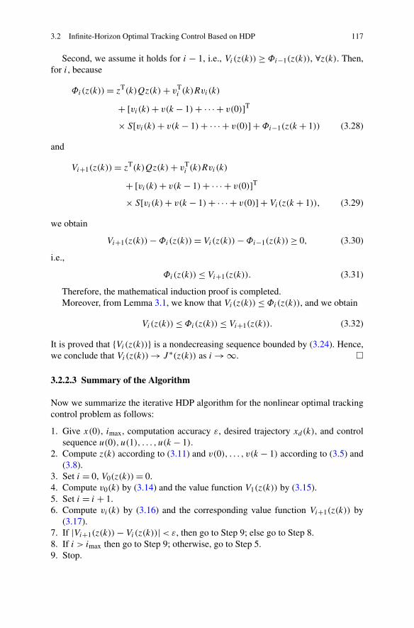
3.2 Infinite-Horizon Optimal Tracking Control Based on HDP 117
Second, we assume it holds for i − 1, i.e., Vi(z(k)) ≥ Φi−1(z(k)), ∀z(k). Then,for i, because
Φi(z(k))= zT(k)Qz(k)+ vTi (k)Rvi(k)
+ [vi(k)+ v(k − 1)+ · · · + v(0)]T
× S[vi(k)+ v(k − 1)+ · · · + v(0)] +Φi−1(z(k + 1)) (3.28)
and
Vi+1(z(k))= zT(k)Qz(k)+ vTi (k)Rvi(k)
+ [vi(k)+ v(k − 1)+ · · · + v(0)]T
× S[vi(k)+ v(k − 1)+ · · · + v(0)] + Vi(z(k + 1)), (3.29)
we obtain
Vi+1(z(k))−Φi(z(k))= Vi(z(k))−Φi−1(z(k))≥ 0, (3.30)
i.e.,
Φi(z(k))≤ Vi+1(z(k)). (3.31)
Therefore, the mathematical induction proof is completed.Moreover, from Lemma 3.1, we know that Vi(z(k))≤Φi(z(k)), and we obtain
Vi(z(k))≤Φi(z(k))≤ Vi+1(z(k)). (3.32)
It is proved that {Vi(z(k))} is a nondecreasing sequence bounded by (3.24). Hence,we conclude that Vi(z(k))→ J ∗(z(k)) as i → ∞. �
3.2.2.3 Summary of the Algorithm
Now we summarize the iterative HDP algorithm for the nonlinear optimal trackingcontrol problem as follows:
1. Give x(0), imax, computation accuracy ε, desired trajectory xd(k), and controlsequence u(0), u(1), . . . , u(k − 1).
2. Compute z(k) according to (3.11) and v(0), . . . , v(k − 1) according to (3.5) and(3.8).
3. Set i = 0, V0(z(k))= 0.4. Compute v0(k) by (3.14) and the value function V1(z(k)) by (3.15).5. Set i = i + 1.6. Compute vi(k) by (3.16) and the corresponding value function Vi+1(z(k)) by
(3.17).7. If |Vi+1(z(k))− Vi(z(k))|< ε, then go to Step 9; else go to Step 8.8. If i > imax then go to Step 9; otherwise, go to Step 5.9. Stop.
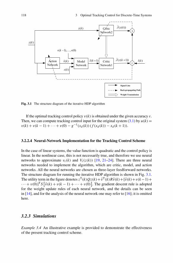
118 3 Optimal Tracking Control for Discrete-Time Systems
Fig. 3.1 The structure diagram of the iterative HDP algorithm
If the optimal tracking control policy v(k) is obtained under the given accuracy ε.Then, we can compute tracking control input for the original system (3.1) by u(k)=v(k)+ v(k − 1)+ · · · + v(0)− g−1(xd(k)) (f (xd(k))− xd(k + 1)).
3.2.2.4 Neural-Network Implementation for the Tracking Control Scheme
In the case of linear systems, the value function is quadratic and the control policy islinear. In the nonlinear case, this is not necessarily true, and therefore we use neuralnetworks to approximate vi(k) and Vi(z(k)) [19, 21–24]. There are three neuralnetworks needed to implement the algorithm, which are critic, model, and actionnetworks. All the neural networks are chosen as three-layer feedforward networks.The structure diagram for running the iterative HDP algorithm is shown in Fig. 3.1.The utility term in the figure denotes zT(k)Qz(k)+ vT(k)Rv(k)+[v(k)+v(k−1)+· · · + v(0)]TS
[v(k)+ v(k − 1)+ · · · + v(0)
]. The gradient descent rule is adopted
for the weight update rules of each neural network, and the details can be seenin [14], and for the analysis of the neural network one may refer to [16]; it is omittedhere.
3.2.3 Simulations
Example 3.4 An illustrative example is provided to demonstrate the effectivenessof the present tracking control scheme.
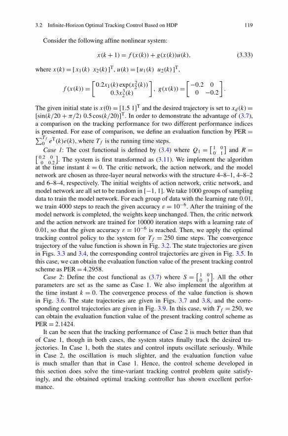
3.2 Infinite-Horizon Optimal Tracking Control Based on HDP 119
Consider the following affine nonlinear system:
x(k + 1)= f (x(k))+ g(x(k))u(k), (3.33)
where x(k)= [x1(k) x2(k) ]T, u(k)= [u1(k) u2(k) ]T,
f (x(k))=[
0.2x1(k) exp(x22(k))
0.3x32(k)
], g(x(k))=
[−0.2 00 −0.2
].
The given initial state is x(0)= [1.5 1]T and the desired trajectory is set to xd(k)=[sin(k/20 + π/2) 0.5 cos(k/20)]T. In order to demonstrate the advantage of (3.7),a comparison on the tracking performance for two different performance indicesis presented. For ease of comparison, we define an evaluation function by PER =∑Tf
0 eT(k)e(k), where Tf is the running time steps.Case 1: The cost functional is defined by (3.4) where Q1 = [ 1 0
0 1
]and R =[ 0.2 0
0 0.2
]. The system is first transformed as (3.11). We implement the algorithm
at the time instant k = 0. The critic network, the action network, and the modelnetwork are chosen as three-layer neural networks with the structure 4–8–1, 4–8–2and 6–8–4, respectively. The initial weights of action network, critic network, andmodel network are all set to be random in [−1,1]. We take 1000 groups of samplingdata to train the model network. For each group of data with the learning rate 0.01,we train 4000 steps to reach the given accuracy ε = 10−6. After the training of themodel network is completed, the weights keep unchanged. Then, the critic networkand the action network are trained for 10000 iteration steps with a learning rate of0.01, so that the given accuracy ε = 10−6 is reached. Then, we apply the optimaltracking control policy to the system for Tf = 250 time steps. The convergencetrajectory of the value function is shown in Fig. 3.2. The state trajectories are givenin Figs. 3.3 and 3.4, the corresponding control trajectories are given in Fig. 3.5. Inthis case, we can obtain the evaluation function value of the present tracking controlscheme as PER = 4.2958.
Case 2: Define the cost functional as (3.7) where S = [ 1 00 1
]. All the other
parameters are set as the same as Case 1. We also implement the algorithm atthe time instant k = 0. The convergence process of the value function is shownin Fig. 3.6. The state trajectories are given in Figs. 3.7 and 3.8, and the corre-sponding control trajectories are given in Fig. 3.9. In this case, with Tf = 250, wecan obtain the evaluation function value of the present tracking control scheme asPER = 2.1424.
It can be seen that the tracking performance of Case 2 is much better than thatof Case 1, though in both cases, the system states finally track the desired tra-jectories. In Case 1, both the states and control inputs oscillate seriously. Whilein Case 2, the oscillation is much slighter, and the evaluation function valueis much smaller than that in Case 1. Hence, the control scheme developed inthis section does solve the time-variant tracking control problem quite satisfy-ingly, and the obtained optimal tracking controller has shown excellent perfor-mance.
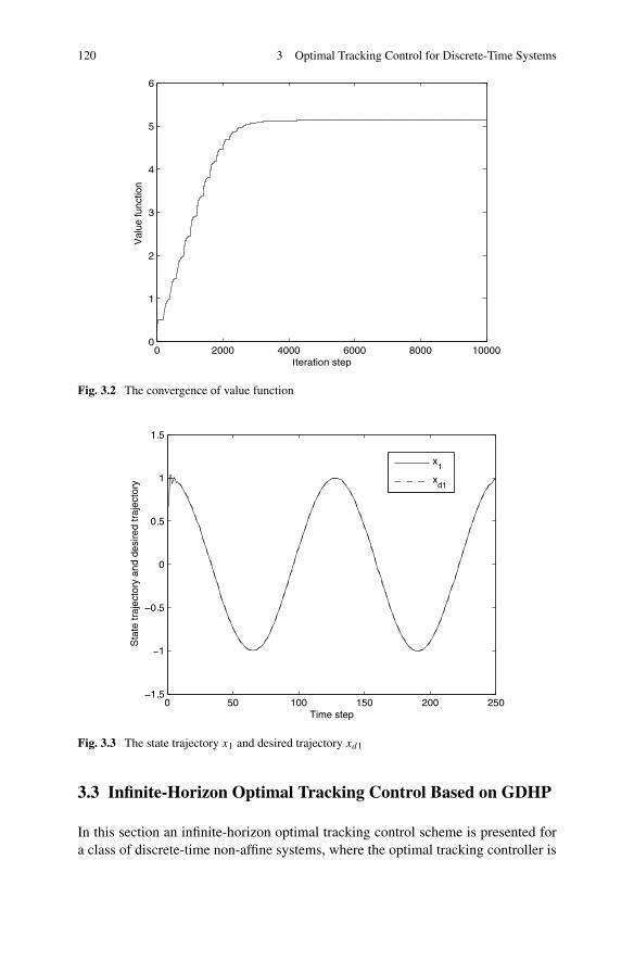
120 3 Optimal Tracking Control for Discrete-Time Systems
Fig. 3.2 The convergence of value function
Fig. 3.3 The state trajectory x1 and desired trajectory xd1
3.3 Infinite-Horizon Optimal Tracking Control Based on GDHP
In this section an infinite-horizon optimal tracking control scheme is presented fora class of discrete-time non-affine systems, where the optimal tracking controller is
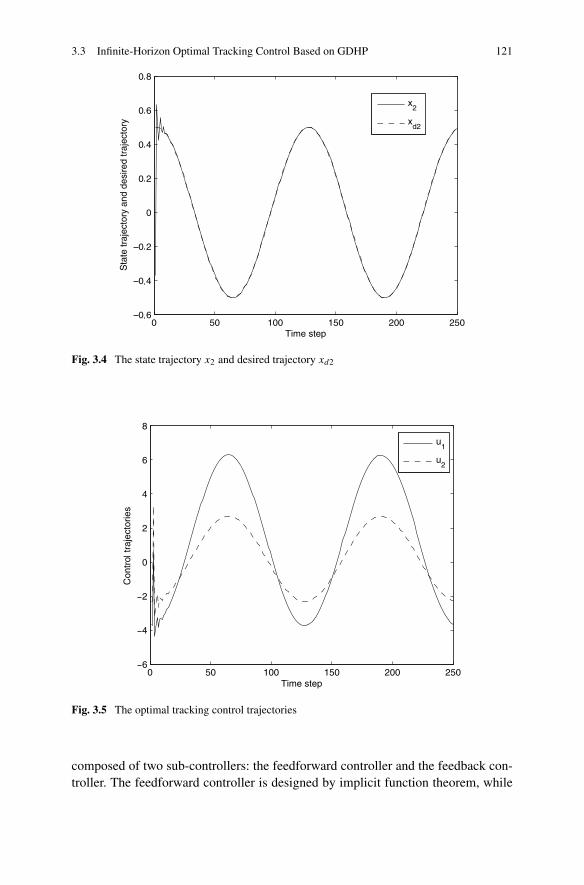
3.3 Infinite-Horizon Optimal Tracking Control Based on GDHP 121
Fig. 3.4 The state trajectory x2 and desired trajectory xd2
Fig. 3.5 The optimal tracking control trajectories
composed of two sub-controllers: the feedforward controller and the feedback con-troller. The feedforward controller is designed by implicit function theorem, while
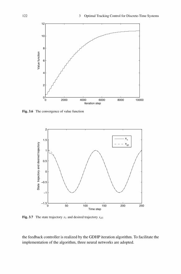
122 3 Optimal Tracking Control for Discrete-Time Systems
Fig. 3.6 The convergence of value function
Fig. 3.7 The state trajectory x1 and desired trajectory xd1
the feedback controller is realized by the GDHP iteration algorithm. To facilitate theimplementation of the algorithm, three neural networks are adopted.
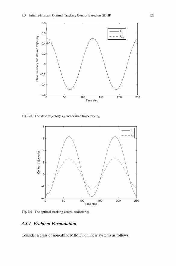
3.3 Infinite-Horizon Optimal Tracking Control Based on GDHP 123
Fig. 3.8 The state trajectory x2 and desired trajectory xd2
Fig. 3.9 The optimal tracking control trajectories
3.3.1 Problem Formulation
Consider a class of non-affine MIMO nonlinear systems as follows:
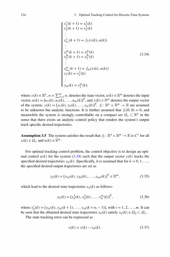
124 3 Optimal Tracking Control for Discrete-Time Systems
⎧⎪⎪⎪⎪⎪⎪⎪⎪⎪⎪⎪⎪⎪⎪⎪⎪⎪⎪⎪⎪⎪⎪⎨
⎪⎪⎪⎪⎪⎪⎪⎪⎪⎪⎪⎪⎪⎪⎪⎪⎪⎪⎪⎪⎪⎪⎩
x11(k + 1)= x1
2(k)
x12(k + 1)= x1
3(k)...
x1n1(k + 1)= f1(x(k), u(k))
...
xm1 (k + 1)= xm2 (k)
xm2 (k + 1)= xm3 (k)...
xmnm(k + 1)= fm(x(k), u(k))
y1(k)= x11(k)
...
ym(k)= xm1 (k),
(3.34)
where x(k) ∈Rn, n=∑m
i=1 ni denotes the state vector, u(k) ∈ Rm denotes the input
vector, u(k)= [u1(k), u2(k), . . . , um(k)]T, and y(k) ∈Rm denotes the output vector
of the system, y(k) = [y1(k), y2(k), . . . , ym(k)]T. fi : Rn × Rm → R are assumed
to be unknown but analytic functions. It is further assumed that fi(0,0) = 0, andmeanwhile the system is strongly controllable on a compact set Ωx ⊂ R
n in thesense that there exists an analytic control policy that renders the system’s outputtrack specific desired trajectories.
Assumption 3.5 The system satisfies the result that fi : Rn ×Rm →R is C1 for all
x(k) ∈Ωx and u(k) ∈Rm.
For optimal tracking control problem, the control objective is to design an opti-mal control u(k) for the system (3.34) such that the output vector y(k) tracks thespecified desired trajectories yd(k). Specifically, it is assumed that for k = 0,1, . . . ,the specified desired output trajectories are set as
yd(k)= [y1d(k), y2d(k), . . . , ymd(k)]T ∈ Rm, (3.35)
which lead to the desired state trajectories xd(k) as follows:
xd(k)= [x1d(k), x
2d(k), . . . , x
md (k)]T, (3.36)
where xid(k)= [yid(k), yid(k+ 1), . . . , yid(k+ni − 1)], with i = 1,2, . . . ,m. It canbe seen that the obtained desired state trajectories xd(k) satisfy xd(k) ∈Ωd ⊂Ωx .
The state tracking error can be expressed as
e(k)= x(k)− xd(k). (3.37)
3.3 Infinite-Horizon Optimal Tracking Control Based on GDHP 125
As is known, for infinite-horizon state feedback control problem, the cost func-tional is generally defined as the following quadratic form:
J (e(0), u)=∞∑
k=0
{xT(k)Q1x(k)+ uT(k)Ru(k)
}, (3.38)
where Q1 ∈ Rn×n and R ∈ R
m×m are positive definite matrices.However, for the infinite-horizon tracking control problem, the cost functional
cannot similarly be defined as
J (e(0), u)=∞∑
k=0
{eT(k)Q1e(k)+ uT(k)Ru(k)
}. (3.39)
Because zero tracking error may not necessarily lead to zero control signals u(k),which implies that this cost functional J (e(0), u) may become infinite.
To overcome the difficulty related to the cost functional, we need to find an idealcontrol, required for maintaining the tracking in steady-state stage. Then, via sub-tracting this ideal control from the control signal u(k), the remaining control signalis allowed to vanish in the steady-state stage. Denote the ideal control signal uf (k);it will be called the feedforward control in the sequel. Further, denote the remainingcontrol signal as v(k), calling it the feedback control. Therefore, the controller u(k)becomes u(k) = v(k)+ uf (k), where uf (k) is to maintain the tracking error closeto zero at the steady-state stage, while v(k) is to stabilize the state tracking error dy-namics at transient stage and vanish in the steady-state stage. In this way, by usingvT(k)Rv(k) to replace uT(k)Ru(k) in the cost functional (3.39), the obtained newcost functional can be finite, and accordingly the optimal tracking control problemcan be appropriately defined.
Moreover, in order to further consider the control signal in the varying process,we add a new term (v(k)−v(k−1))TS(v(k)−v(k−1)) to the cost functional (3.39).Specifically, a new cost functional is defined as
J (e(k), v)=∞∑
i=k
{eT(i)Q1e(i)+ vT(i)Rv(i)
+ (v(i)− v(i − 1))T S (v(i)− v(i − 1))}, (3.40)
where Q1 ∈ Rn×n, R ∈ R
m×m and S ∈ Rm×m are all positive definite, v(k) is the
feedback control satisfying v(k)= 0 for k < 0.After defining the cost functional (3.40), in the following development, we will
focus on the optimal tracking controller design. It can be seen that the optimal con-troller is composed of two sub-controllers, i.e., the feedforward control uf (k) andthe feedback control v(k). In order to design these sub-controllers, we first derivethe error system.
For convenience of analysis, the system (3.34) can be rewritten as
x(k + 1)= F(x(k), u(k)), (3.41)
126 3 Optimal Tracking Control for Discrete-Time Systems
where F : Rn ×Rm → R
n is the vector function describing the nonlinear dynamicsof the system (3.34).
In view of
e(k + 1)= x(k + 1)− xd(k + 1), (3.42)
one has
e(k + 1)= F(x(k), u(k))− xd(k + 1). (3.43)
Since u(k)= v(k)+ uf (k), the error equation can be reformulated as
e(k + 1)= F(e(k)+ xd(k), v(k)+ uf (k)
)− xd(k + 1). (3.44)
Keeping (3.42) in mind, once the error system (3.44) is stabilized, i.e., e → 0, thestate vector of the original system will track the desired trajectories simultaneously.Since the feedforward control uf (k) is designed beforehand to keep the state vectorof the plant to the desired trajectories at the steady-state stage, it first is required tostabilize the error dynamic by choosing an appropriate feedback control v(k).
Therefore, based on the above analysis, the optimal tracking control problem of(3.34) has been converted into two problems: one is to compute the feedforwardcontrol uf (k), and the other is to design the optimal feedback control v(k) for sta-bilizing the error equation (3.44). In the following development, we will discuss thefeedforward controller design and the optimal feedback controller design in detail.
3.3.2 Infinite-Horizon Optimal Tracking Control Based on GDHP
3.3.2.1 Design and Implementation of Feedforward Controller
As mentioned above, in order to make a plant follow specific desired trajectories,it is necessary to design the feedforward controller uf (k) so that the tracking errorcan keep zero at the steady-state stage. Therefore, by substituting the desired statexd(k) and the ideal feedforward control uf (k) in place of x(k) and u(k) in (3.34),the ideal steady-state equation can be written as
⎧⎪⎪⎪⎨
⎪⎪⎪⎩
x1n1d
(k + 1)= f1(xd(k), uf (k))
x2n2d
(k + 1)= f2(xd(k), uf (k))
...
xmnmd(k + 1)= fm(xd(k), uf (k)),
(3.45)
where the ideal feedforward control uf (k) is left to be solved in the following part.Let
xnd(k + 1)= [x1n1d
(k + 1), x2n2d
(k + 1), . . . , xmnmd(k + 1)]T. (3.46)
3.3 Infinite-Horizon Optimal Tracking Control Based on GDHP 127
Then the ideal steady-state equation (3.45) can further be written as
xnd(k + 1)= F(xd(k), uf (k)), (3.47)
where F : Rn ×Rm → R
m is the vector function defined as
F(·)= [f1(·), f2(·), . . . , fm(·)
]T.
To solve the ideal feedforward control uf (k) uniquely from the above equa-tion (3.47), we need to make sure that the implicit function theorem holds aroundthe desired trajectories xd(k). Therefore, we first present an assumption as follows.
Assumption 3.6 The Jacobian matrix Υ of the system (3.34) is nonsingular for allx(k) ∈Ωd,u(k) ∈R
m, where
Υ =
⎡
⎢⎢⎢⎢⎣
∂f1(x(k),u(k))∂u1(k)
∂f1(x(k),u(k))∂u2(k)
. . .∂f1(x(k),u(k))
∂um(k)∂f2(x(k),u(k))
∂u1(k)∂f2(x(k),u(k))
∂u2(k). . .
∂f2(x(k),u(k))∂um(k)
......
...∂fm(x(k),u(k))
∂u1(k)∂fm(x(k),u(k))
∂u2(k). . .
∂fm(x(k),u(k))∂um(k)
⎤
⎥⎥⎥⎥⎦. (3.48)
Based on Assumptions 3.5 and 3.6, the implicit function theorem is obviouslyensured to hold. Therefore, the ideal feedforward control input uf (k) uniquely ex-ists around the specific desired state trajectories xd(k) ∈ Ωd and can further be ex-pressed as follows:
uf (k)=G(xd(k), xnd(k + 1)), (3.49)
where G : Rn × Rm → R is a unique one-to-one differentiable vector function sat-
isfying xnd(k + 1)= F(xd(k),G(xd(k), xnd(k + 1))).
3.3.2.2 Design and Implementation of Optimal Feedback Controller
The feedforward control has already been presented in the above subsection, whichis the unique control input required at steady-state stage. The crucial problem leftto solve is to design the optimal feedback control by the iterative algorithm afterperforming some transformation on the error system (3.44).
System Transformation
With the feedforward control uf (k) in (3.49), we substitute it into the error equation(3.44) and obtain
e(k + 1)= F (e(k)+ xd(k), v(k)+G(xd(k), xnd(k + 1)))− xd(k + 1).
(3.50)
128 3 Optimal Tracking Control for Discrete-Time Systems
From (3.36), we can know that xd(k) is only denoting the desired trajectory. It isassumed that the desired trajectory is generated by the following relationship:
xd(k + 1)= δ(xd(k)), (3.51)
where δ(·) = [δ1(·), δ2(·), . . . , δn(·)]T is an analytic vector function. Then, it isstraightforward to show from (3.51) that
xnd(k + 1)= [δn1(xd(k)), δn1+n2(xd(k)), . . . , δn(xd(k))].
Therefore, the error system (3.50) can further be written as
e(k + 1)= Γ (e(k), xd(k), v(k)). (3.52)
In the above equation, e(k) is the states of the error equation and xd(k) can betreated as signals. However, they are time-varying. To the best of our knowledge, itis still not clear in the literature how to obtain the analytical solution for the optimalcontrol of the above systems with time-varying signals. Inspired by the dimensionaugmentation technique, in this section we will construct an augmented system toequivalently solve the optimal feedback control v(k).
Define z1(k)= e(k) and z2(k)= xd(k), and then the error system (3.52) and thedesired state trajectories equation (3.51) can be rewritten as
{z1(k + 1)= Γ (z1(k), z2(k), v(k))
z2(k + 1)= δ(z2(k)),(3.53)
which is called the augmented system of the error system (3.50). Here, the argu-ments z1(k) and z2(k) are viewed as two new state vectors of the augmented sys-tem. By this augmentation, the augmented system (3.53) has higher dimension thanthe original error system (3.52), and there is no time variable explicitly appearingin (3.53).
Accordingly, for this augmented system, the cost functional (3.40) can be rede-fined as
J (z(k), v)=∞∑
t=k
{zT(t)Qz(t)+ vT(t)Rv(t) (3.54)
+ (v(t)− v(t − 1))T S (v(t)− v(t − 1))},
where z(t) = [eT(t) xTd (t)]T ∈ R
2n and Q = [ Q1 0n×n
0n×n 0n×n
] ∈ R2n×2n. This cost func-
tional (3.54) is equivalent to (3.40) in the sense that the objectives of the two costfunctionals are the same.
With this augmented model (3.53), it is now possible to design the optimal feed-back controller to guarantee that the cost functional (3.54) is finite.
3.3 Infinite-Horizon Optimal Tracking Control Based on GDHP 129
The Optimal Feedback Controller Design Based on GDHP Algorithm
In order to solve the optimal feedback control problem, the admissible control isdefined similarly as Definition 2.1. However, the state vector is z(k) and the costfunctional is J (z(0), v).
Actually the cost functional (3.54) can be expanded as
J (z(k), v)= zT(k)Qz(k)+ vT(k)Rv(k)
+ (v(k)− v(k − 1))T S (v(k)− v(k − 1))
+ J (z(k + 1), v). (3.55)
From Bellman’s optimality principle, the HJB equation is
J ∗(z(k))= minv(k)
{zT(k)Qz(k)+ vT(k)Rv(k)
+ (v(k)− v(k − 1))T S(v(k)− v(k − 1)
)
+ J ∗(z(k + 1))}, (3.56)
where J ∗(z(k)) is the optimal value function.The corresponding optimal control can be defined as
u∗(k)= arg minv(k)
{zT(k)Qz(k)+ vT(k)Rv(k)
+ (v(k)− v(k − 1))T S(v(k)− v(k − 1)
)
+ J ∗(z(k + 1))}. (3.57)
It should be noted that if the optimal value function J ∗(z(k)) can be solved fromHJB equation (3.56), the optimal feedback control u∗(k) can be computed. How-ever, it is not straightforward to solve this HJB equation in most cases. Thus, in thissection, we propose a new iterative algorithm named GDHP algorithm to solve theoptimal control by introducing a new vector λi(z(k)).
First, we start with the initial value function V0(·) = 0, initial costate functionλ0(·)= 0, and then for i = 0,1, . . . we implement the iteration between
vi(k)= arg minv(k)
{zT(k)Qz(k)+ vT(k)Rv(k)
+ (v(k)− v(k − 1))T S (v(k)− v(k − 1))
+ Vi(z(k + 1))}
(3.58)
130 3 Optimal Tracking Control for Discrete-Time Systems
i.e.,
vi(k)= − 1
2(R + S)−1
(− 2Sv(k − 1)+
(dz(k + 1)
dvi(k)
)T
λi(z(k + 1))
)(3.59)
and
Vi+1(z(k))= zT(k)Qz(k)+ vTi (k)Rvi(k)
+ (vi(k)− v(k − 1))T S (vi(k)− v(k − 1))
+ Vi(z(k + 1)
), (3.60)
λi+1(z(k))= 2Qz(k)+(∂z(k + 1)
∂z(k)
)T
λi(z(k + 1)). (3.61)
From the above analysis, we can find that via the costate function sequence(3.61), the optimal control sequence can be directly obtained by (3.59), which canavoid computing ∂Vi(z(k + 1))/∂z(k + 1) at each iterative step. This explains theworking principle for the present GDHP algorithm.
Convergence Analysis of GDHP Algorithm
In the following we will present a concise convergence analysis of the iterationamong (3.58), (3.60) and (3.61) with Vi(z(k)) → J ∗(z(k)), λi(z(k)) → λ∗(z(k))and the control policy vi(k)→ u∗(k) as i → ∞.
Lemma 3.7 Let μi be any sequence of control policies, and vi is the optimal poli-cies by (3.58). Define Vi+1(z(k)) as (3.60) and Λi+1(z(k)) as
Λi+1(z(k))= zT(k)Qz(k)+μTi (k)Rμi(k)
+ (μi(k)− v(k − 1))T S (μi(k)− v(k − 1))
+Λi(z(k + 1)). (3.62)
If V0(·)=Λ0(·)= 0, then Vi(z(k))≤Λi(z(k)), ∀i.
Lemma 3.8 For the sequence {Vi(z(k))} defined by (3.60), if the system (3.52) iscontrollable, then there is an upper bound Y such that 0 ≤ Vi ≤ Y , ∀i.
With Lemma 3.7 and Lemma 3.8, we are now ready to present the main theorem.
Theorem 3.9 Define the sequence {Vi(z(k))} as (3.60), with V0(·) = 0, the se-quence {λi(z(k))} as (3.61), with λ0(·) = 0. Then, {Vi(z(k))} is a nondecreasing
3.3 Infinite-Horizon Optimal Tracking Control Based on GDHP 131
sequence satisfying Vi+1(z(k))≥ Vi(z(k)), ∀i, and converges to the optimal valuefunction of the discrete-time HJB equation (3.56), i.e., Vi(z(k)) → J ∗(z(k)) asi → ∞. Meanwhile, the costate function and the control input sequences are con-vergent, with λi(z(k))→ λ∗(z(k)) and vi(k)→ u∗(k) as i → ∞.
Proof For the convenience of analysis, define a new sequence {Φi(z(k))} as follows:
Φi+1(z(k))= zT(k)Qz(k)+ vTi+1(k)Rvi+1(k)
+ (vi+1(k)− v(k − 1))TS(vi+1(k)− v(k − 1))
+Φi(z(k + 1)), (3.63)
where vi(k) defined by (3.58) and Φ0(·)= V0(·)= 0.In the following, we prove Φi(z(k)) ≤ Vi+1(z(k)) by mathematical induction.
First, we prove that it holds for i = 0. Noting that
V1(z(k))−Φ0(z(k))= zT(k)Qz(k)+ vT0 (k)Rv0(k)
+ (v0(k)− v(k − 1))TS(v0(k)− v(k − 1))
≥ 0, (3.64)
for i = 0, we get
V1(z(k))≥Φ0(z(k)). (3.65)
Second, we assume that it holds for i − 1, i.e., Vi(z(k))≥Φi−1(z(k)), ∀z(k). Then,for i, since
Φi(z(k))= zT(k)Qz(k)+ vTi (k)Rvi(k)
+ (vi(k)− v(k − 1))TS(vi(k)− v(k − 1))
+Φi−1(z(k + 1)), (3.66)
and
Vi+1(z(k))= zT(k)Qz(k)+ vTi (k)Rvi(k)
+ (vi(k)− v(k − 1))TS(vi(k)− v(k − 1))
+ Vi(z(k + 1)), (3.67)
we obtain
Vi+1(z(k))−Φi(z(k))= Vi(z(k))−Φi−1(z(k))≥ 0, (3.68)
i.e.,
Φi(z(k))≤ Vi+1(z(k)). (3.69)
Therefore, the mathematical induction proof is completed.
132 3 Optimal Tracking Control for Discrete-Time Systems
Moreover, from Lemma (3.7), we know that Vi(z(k)) ≤ Φi(z(k)); therefore weobtain
Vi(z(k))≤Φi(z(k))≤ Vi+1(z(k)), (3.70)
which proves that {Vi(z(k))} is a bounded nondecreasing sequence. Hence we con-clude that Vi(z(k)) → J ∗(z(k)) as i → ∞. With λi(z(k)) = ∂Vi(z(k))/∂z(k) andλ∗(z(k))= ∂J ∗(z(k))/∂z(k), the corresponding costate sequence {λi(z(k))} is alsoconvergent with λi(z(k)) → λ∗(z(k)) as i → ∞. Since the costate functions areconvergent, we conclude that the corresponding control sequence vi(k) convergesto the optimal control u∗(k) as i → ∞.
This completes the proof. �
Neural-Network Implementation of the Optimal Feedback Controller
For facilitating the implementation of the GDHP algorithm, we use three neuralnetworks, named model network, critic network, and action network, respectively.
Model Network
Before carrying out the iterative process, we first construct the model network toapproximate the nonlinear dynamic of the augmented system. The model networkpredicts z(k+1) given z(k) and v(k), i.e., it learns the mapping given in (3.53). Theoutput of the model network is denoted
z(k + 1)=WTmφ(V
TmIm(k)), (3.71)
where Im(k)= col {v(k), z(k)} is the input vector of the model network.Define the output error of the network as
em(k)= z(k + 1)− z(k + 1). (3.72)
The weights in the model network are updated to minimize the following perfor-mance error measure:
Em(k)= 1
2eTm(k)em(k). (3.73)
The weight update rule for model network is chosen as a gradient-based adaptationgiven by
Wm(j + 1)=Wm(j)− αm(j)
[∂Em(k)
∂Wm
], (3.74)
Vm(j + 1)= Vm(j)− αm(j)
[∂Em(k)
∂Vm
], (3.75)
where αm(j) is the learning rate of the model network.After the model network is trained, its weights are kept unchanged.
3.3 Infinite-Horizon Optimal Tracking Control Based on GDHP 133
Critic Network
The output of the critic network is composed of two parts; one part is used to ap-proximate the index function Vi+1(k), and the other part is used to approximatethe costate function λi+1(k). Define the output of the critic network as Oc(i+1)(k),which can be described by
Oc(i+1)(k)=WTc(i+1)φ(V
Tc(i+1)z(k)). (3.76)
Define the output target of the critic network as Dc(i+1)(k), which is also com-posed of two parts, i.e.,
Dc(i+1)(k)= [Vi+1(k) λi+1(k)]T, (3.77)
where Vi+1(k) is the target of value function computed by (3.60); λi+1(k) is thetarget of the costate function computed by (3.61), respectively.
Define the error function for the critic network as
ec(i+1)(k)=Oc(i+1)(k)−Dc(i+1)(k). (3.78)
Also, define the objective function to be minimized in the critic network as
Ec(i+1)(k)= 1
2eTc(i+1)(k)ec(i+1)(k). (3.79)
Choose the weight update rule for the critic network as a gradient-based rule givenby
Wc(i+1)(j + 1)=Wc(i+1)(j)− αc(j)
[∂Ec(i+1)(k)
∂Wc(i+1)
], (3.80)
Vc(i+1)(j + 1)= Vc(i+1)(j)− αc(j)
[∂Ec(i+1)(k)
∂Vc(i+1)
], (3.81)
where αc(j) > 0 is the learning rate of critic network.
Action Network
In the action network the augmented vector z(k) is used as input to create the optimalfeedback control as the output of the network. The output can be formulated as
vi (k)=WTaiφ(V
Taiz(k)). (3.82)
The output target vi(k) is given by (3.59). Thus, we can define the output error ofthe action network as
eai(k)= vi (k)− vi(k). (3.83)
134 3 Optimal Tracking Control for Discrete-Time Systems
The weights in the action network are updated to minimize the following perfor-mance error measure:
Eai(k)= 1
2eTai(k)eai(k). (3.84)
The update algorithm is then similar to the one in the critic network. By the gradientdescent rule, we have
Wai(j + 1)=Wai(j)− αa(j)
[∂Eai(k)
∂Wai
], (3.85)
Vai(j + 1)= Vai(j)− αa(j)
[∂Eai(k)
∂Vai
], (3.86)
where αa(j) > 0 is the learning rate of action network.
Design Procedure of the Optimal Tracking Controller
The procedures of the optimal tracking control scheme based on the GI-GDHP al-gorithm are summarized as follows:
1. Given x(0), u(0), u(1), . . . , u(k− 1), imax, ε0, and the desired trajectory yd(k).2. Compute xd(k), xd(k + 1), z(k) according to (3.36) and (3.37).3. Compute the feedforward control uf (k) by solving the implicit equation
xnd(k + 1)= F(xd(k), uf (k)).4. Construct the model network z(k+1)=WT
mφ(VTmIm(k)) with the initial weight
parameters chosen randomly from [−0.1,0.1] and train the model network witha random input vector uniformly distributed in the interval [−1,1] and an arbi-trary initial state vector till the given accuracy ε0 is reached.
5. Set the iterative step i = 0, the initial value function Vi(·)= 0 and costate func-tion λi(·) = 0. Construct both the critic network and the action network withthe initial weight parameters chosen randomly from [−1,1].
6. Compute the output target by (3.59) and update the weight parameters of theaction network by (3.85) and (3.86).
7. Compute the output target by (3.77) and update the weight parameters of thecritic network by (3.80) and (3.81).
8. If
‖λi+1(z(k))− λi(z(k))‖2 + ‖Vi+1(z(k))− Vi(z(k))‖2 < ε0,
go to Step 9; otherwise i = i + 1, go to Step 6.9. If i > imax, v(k)= vi(k) and go to Step 11; otherwise i = i + 1, go to Step 6.
10. Compute the approximate optimal control u(k)= v(k)+ uf (k).11. Stop.
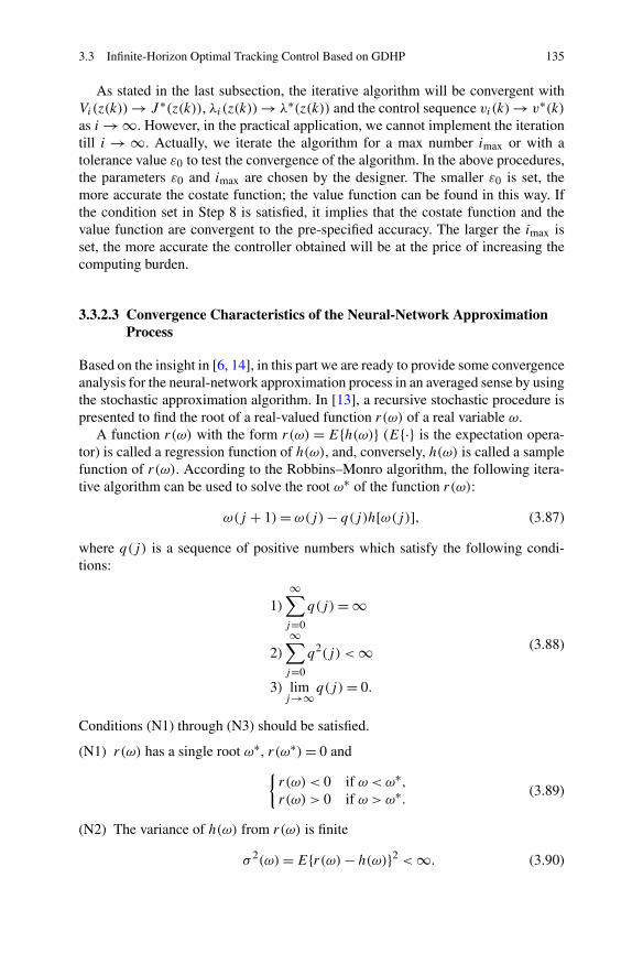
3.3 Infinite-Horizon Optimal Tracking Control Based on GDHP 135
As stated in the last subsection, the iterative algorithm will be convergent withVi(z(k))→ J ∗(z(k)), λi(z(k))→ λ∗(z(k)) and the control sequence vi(k)→ v∗(k)as i → ∞. However, in the practical application, we cannot implement the iterationtill i → ∞. Actually, we iterate the algorithm for a max number imax or with atolerance value ε0 to test the convergence of the algorithm. In the above procedures,the parameters ε0 and imax are chosen by the designer. The smaller ε0 is set, themore accurate the costate function; the value function can be found in this way. Ifthe condition set in Step 8 is satisfied, it implies that the costate function and thevalue function are convergent to the pre-specified accuracy. The larger the imax isset, the more accurate the controller obtained will be at the price of increasing thecomputing burden.
3.3.2.3 Convergence Characteristics of the Neural-Network ApproximationProcess
Based on the insight in [6, 14], in this part we are ready to provide some convergenceanalysis for the neural-network approximation process in an averaged sense by usingthe stochastic approximation algorithm. In [13], a recursive stochastic procedure ispresented to find the root of a real-valued function r(ω) of a real variable ω.
A function r(ω) with the form r(ω) = E{h(ω)} (E{·} is the expectation opera-tor) is called a regression function of h(ω), and, conversely, h(ω) is called a samplefunction of r(ω). According to the Robbins–Monro algorithm, the following itera-tive algorithm can be used to solve the root ω∗ of the function r(ω):
ω(j + 1)= ω(j)− q(j)h[ω(j)], (3.87)
where q(j) is a sequence of positive numbers which satisfy the following condi-tions:
1)∞∑
j=0
q(j)= ∞
2)∞∑
j=0
q2(j) <∞
3) limj→∞q(j)= 0.
(3.88)
Conditions (N1) through (N3) should be satisfied.
(N1) r(ω) has a single root ω∗, r(ω∗)= 0 and{r(ω) < 0 if ω < ω∗,r(ω) > 0 if ω > ω∗. (3.89)
(N2) The variance of h(ω) from r(ω) is finite
σ 2(ω)=E{r(ω)− h(ω)}2 <∞. (3.90)
136 3 Optimal Tracking Control for Discrete-Time Systems
(N3) The real-valued function r(ω) satisfies
| r(ω) |<M0 | ω−ω∗ | +M1 <∞. (3.91)
If the iterative algorithm (3.87) is implemented under the conditions (N1) through(N3), the obtained ω(j) will converge toward the true root ω∗ in the mean squareerror sense with probability one, i.e.,
limj→∞E
{‖ ω(j)−ω∗ ‖2
}= 0 (3.92)
Prob
{limj→∞ω(j)= ω∗
}= 1. (3.93)
In this section, similar to the framework in [14], the Robbins–Monro algorithm isapplied by setting r(ω)= ∂E/∂ω, where E is an objective function to be optimized.If E has a local optimum at ω∗, r(ω) will satisfy the condition (N1) locally at ω∗.If E has a quadratic form, r(ω) will satisfy the condition (N1) globally.
First, we are ready to investigate the learning process of action network. Recallthat the instantaneous error measure for the action network is of the following form:
eai(k)= vi (k)− vi(k). (3.94)
The performance error measure is defined as
Eai(k)= 1
2eTai(k)eai(k). (3.95)
Let
Eai =E {Eai} , (3.96)
and assume that the expectation is well defined over the discrete state measurements.The derivative of Eai with respect to the weights of the action network is then of theform
∂Eai
∂ωai=E
{(∂eai
∂ωai
)T
eai
}. (3.97)
According to the Robbins–Monro algorithm, the root (it may be a local root) of∂Eai/∂ωai as a function of ωai can be obtained by the following recursive proce-dure, if the root exists and if the step size αa(j) meets all the requirements describedin (3.88):
ωai(j + 1)= ωai(j)− αa(j)
[(∂eai
∂ωai
)T
eai
]. (3.98)
Recalling the update rule for the action network, we find that (3.98) is equivalentto (3.83)–(3.86). In this sense, the action network update rule of (3.83)–(3.86) is
3.3 Infinite-Horizon Optimal Tracking Control Based on GDHP 137
actually converging to a (local) minimum of the performance measure (3.96) in astatistical average sense.
In a similar framework, the convergence analysis of critic network and modelnetwork in the optimal feedback scheme can be derived, except that the definitionsof the error measures are different. The details are therefore omitted here to savespace.
3.3.3 Simulations
Example 3.10 An example is provided to demonstrate the present effectiveness ofthe optimal tracking control scheme.
Consider the following nonaffine nonlinear system:⎧⎪⎪⎪⎪⎪⎪⎪⎨
⎪⎪⎪⎪⎪⎪⎪⎩
x11(k + 1)= x1
2(k)
x12(k + 1)= 0.4x2
2(k)− 0.3 cos(x12(k))+ 2u1 + 2 tanh(u2)
x21(k + 1)= x2
2(k)
x22(k + 1)= x1
1(k)− 2u2 + 3 sin(x22(k))u1
y1(k)= x11(k)
y2(k)= x21(k),
(3.99)
where x(k) = [x11(k) x
12(k) x
21(k) x
22(k)] ∈ R
4 denotes the state vector, u(k) =[u1(k) u2(k)] ∈ R
2 is the control vector, y(k) = [y1(k) y2(k)] ∈ R2 is the output
vector.The cost functional is defined as (3.54), the weight matrices are set as Q1 = 5I4,
R = 2I2 and S = 2I2, where In denotes the n×n identity matrix. The desired outputtrajectories are set as y1d(k)= 0.5sin[2πk/100], y2d(k)= 0.5cos[2πk/100].
We would like to mention that the above test system (3.99) satisfies Assump-tions 3.5 and 3.6 for the desired trajectories y1d(k), y2d(k). Therefore, the optimaltracking control scheme developed above can be used to design the optimal con-troller for this plant.
Here, the model network, the critic network, and the action network are set asthe feedforward neural networks with the structures of 10–8–8, 8–8–9, and 8–8–2,respectively. All the neural networks are trained with a certain number of trainingcycles, and in each training cycle there are a certain number of iterative steps. Forthe optimal feedback controller design, we should first train the model network.The learning rate is chosen as αm(j) = 0.1(1 − j/Nm), where Nm is the iterativesteps of each training cycle which is set to Nm = 5000. Denote the training cyclenumber of all the neural networks as L. We train the model network for L = 1000cycles with a random input vector uniformly distributed in the interval [−1,1] andan arbitrary initial state vector to get the predefined accuracy εm = 10−4. Then,keeping the weights of the model network fixed, both the critic network and theaction network are trained for L= 200 cycles to reach the predefined accuracy ε0 =10−3. We should mention that in the training of the critic network and the action
138 3 Optimal Tracking Control for Discrete-Time Systems
Fig. 3.10 The convergence trajectory of value function
network, the training cycle number L denotes the outer iterative number i in theGDHP algorithm. The learning rate of the critic network is set as αc(j) = 0.1(1 −j/Nc), where Nc is the iterative steps of each training cycle in critic network. Thelearning rate of action network is set as αa(j) = 0.1(1 − j/Na), where Na is theiterative steps of each training cycle in the action network. In the simulation, we setthe iterative steps as Nc =Na = 200. After simulation, the convergence trajectoriesof the value function and costate function are shown in Figs. 3.10, 3.11. In order tocompare the different actions of the control policies obtained by different trainingcycles, for the same initial state vector x(0) = [−0.2 0.2314 0.3 0.499], we usethe different control policies obtained for the plant and obtain the simulation resultsas follows. The output tracking error trajectories are shown in Figs. 3.12, 3.13, 3.14and 3.15. It can be seen that the controlled plant’s dynamics is out of order whenthe number of training cycles L is less than 12, and when L > 15 the trackingperformance is improved with the training cycles increasing. When L > 120, theiterative process is basically convergent with slight improvement in the trackingperformance.
From the simulation results, we can see that the output trajectories do track thedesired trajectories quite well, so the control scheme developed in this section cansolve the tracking control problem satisfactorily.
3.4 Finite-Horizon Optimal Tracking Control Based on ADP
A finite-horizon neuro-optimal tracking control scheme for a class of discrete-timenonlinear systems is developed in this section. Through a system transformation,
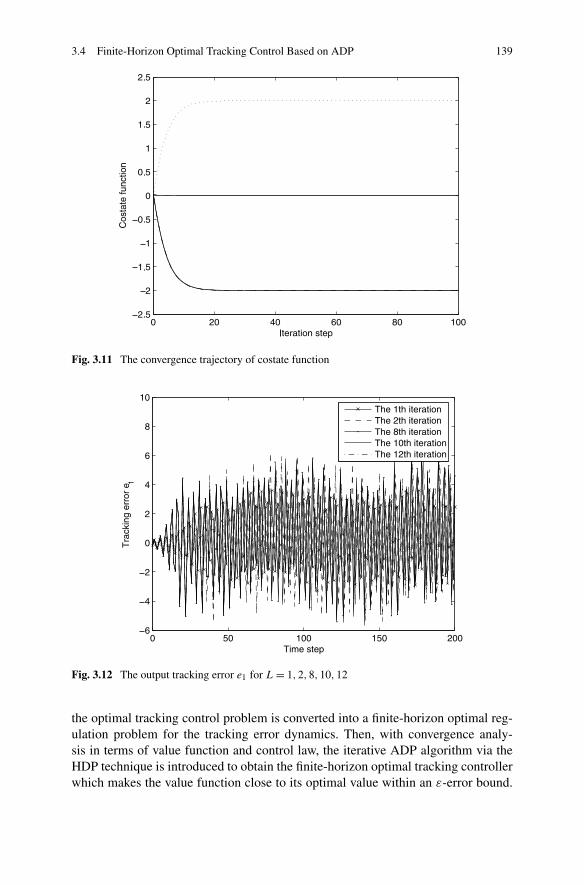
3.4 Finite-Horizon Optimal Tracking Control Based on ADP 139
Fig. 3.11 The convergence trajectory of costate function
Fig. 3.12 The output tracking error e1 for L= 1,2,8,10,12
the optimal tracking control problem is converted into a finite-horizon optimal reg-ulation problem for the tracking error dynamics. Then, with convergence analy-sis in terms of value function and control law, the iterative ADP algorithm via theHDP technique is introduced to obtain the finite-horizon optimal tracking controllerwhich makes the value function close to its optimal value within an ε-error bound.
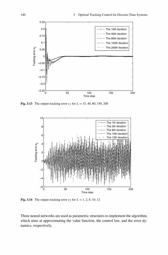
140 3 Optimal Tracking Control for Discrete-Time Systems
Fig. 3.13 The output tracking error e1 for L= 15,40,80,150,200
Fig. 3.14 The output tracking error e2 for L= 1,2,8,10,12
Three neural networks are used as parametric structures to implement the algorithm,which aims at approximating the value function, the control law, and the error dy-namics, respectively.
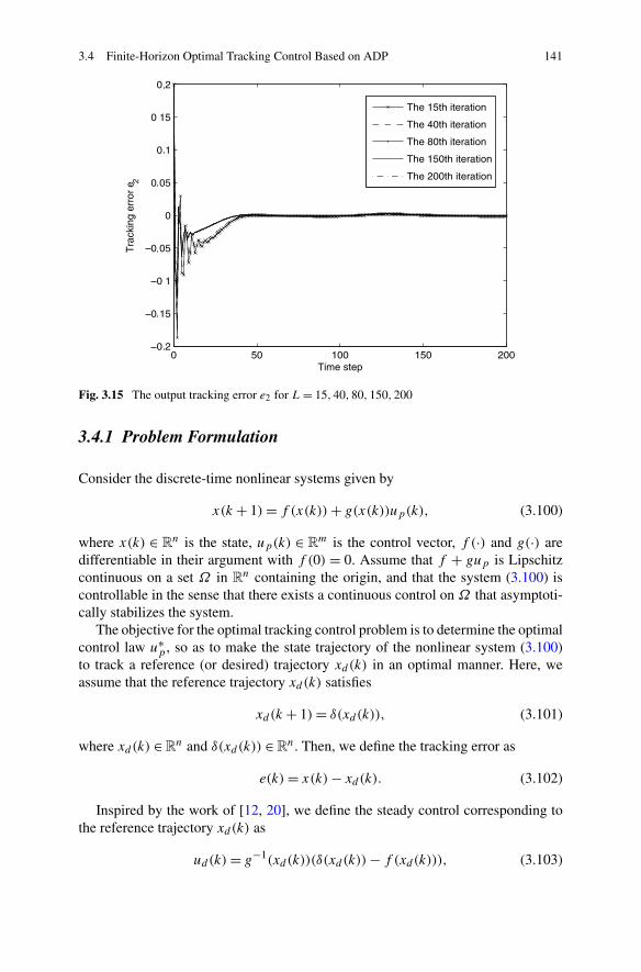
3.4 Finite-Horizon Optimal Tracking Control Based on ADP 141
Fig. 3.15 The output tracking error e2 for L= 15,40,80,150,200
3.4.1 Problem Formulation
Consider the discrete-time nonlinear systems given by
x(k + 1)= f (x(k))+ g(x(k))up(k), (3.100)
where x(k) ∈ Rn is the state, up(k) ∈ R
m is the control vector, f (·) and g(·) aredifferentiable in their argument with f (0) = 0. Assume that f + gup is Lipschitzcontinuous on a set Ω in R
n containing the origin, and that the system (3.100) iscontrollable in the sense that there exists a continuous control on Ω that asymptoti-cally stabilizes the system.
The objective for the optimal tracking control problem is to determine the optimalcontrol law u∗
p , so as to make the state trajectory of the nonlinear system (3.100)to track a reference (or desired) trajectory xd(k) in an optimal manner. Here, weassume that the reference trajectory xd(k) satisfies
xd(k + 1)= δ(xd(k)), (3.101)
where xd(k) ∈ Rn and δ(xd(k)) ∈R
n. Then, we define the tracking error as
e(k)= x(k)− xd(k). (3.102)
Inspired by the work of [12, 20], we define the steady control corresponding tothe reference trajectory xd(k) as
ud(k)= g−1(xd(k))(δ(xd(k))− f (xd(k))), (3.103)
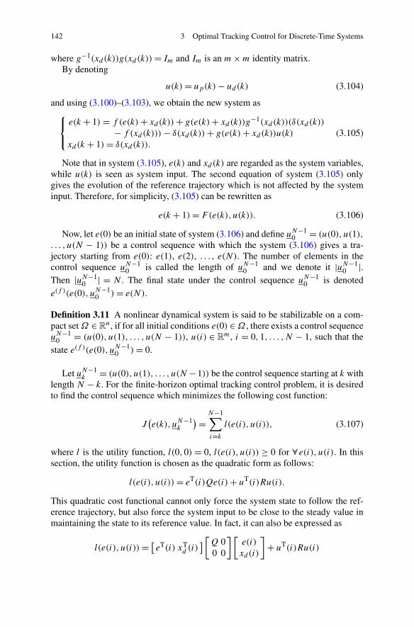
142 3 Optimal Tracking Control for Discrete-Time Systems
where g−1(xd(k))g(xd(k))= Im and Im is an m×m identity matrix.By denoting
u(k)= up(k)− ud(k) (3.104)
and using (3.100)–(3.103), we obtain the new system as⎧⎨
⎩
e(k + 1) = f (e(k)+ xd(k))+ g(e(k)+ xd(k))g−1(xd(k))(δ(xd(k))
− f (xd(k)))− δ(xd(k))+ g(e(k)+ xd(k))u(k)
xd(k + 1)= δ(xd(k)).
(3.105)
Note that in system (3.105), e(k) and xd(k) are regarded as the system variables,while u(k) is seen as system input. The second equation of system (3.105) onlygives the evolution of the reference trajectory which is not affected by the systeminput. Therefore, for simplicity, (3.105) can be rewritten as
e(k + 1)= F(e(k), u(k)). (3.106)
Now, let e(0) be an initial state of system (3.106) and define uN−10 = (u(0), u(1),
. . . , u(N − 1)) be a control sequence with which the system (3.106) gives a tra-jectory starting from e(0): e(1), e(2), . . . , e(N). The number of elements in thecontrol sequence uN−1
0 is called the length of uN−10 and we denote it |uN−1
0 |.Then |uN−1
0 | = N . The final state under the control sequence uN−10 is denoted
e(f )(e(0), uN−10 )= e(N).
Definition 3.11 A nonlinear dynamical system is said to be stabilizable on a com-pact set Ω ∈R
n, if for all initial conditions e(0) ∈Ω , there exists a control sequenceuN−1
0 = (u(0), u(1), . . . , u(N − 1)), u(i) ∈ Rm, i = 0,1, . . . ,N − 1, such that the
state e(f )(e(0), uN−10 )= 0.
Let uN−1k = (u(0), u(1), . . . , u(N −1)) be the control sequence starting at k with
length N − k. For the finite-horizon optimal tracking control problem, it is desiredto find the control sequence which minimizes the following cost function:
J(e(k), uN−1
k
)=N−1∑
i=k
l(e(i), u(i)), (3.107)
where l is the utility function, l(0,0) = 0, l(e(i), u(i)) ≥ 0 for ∀ e(i), u(i). In thissection, the utility function is chosen as the quadratic form as follows:
l(e(i), u(i))= eT(i)Qe(i)+ uT(i)Ru(i).
This quadratic cost functional cannot only force the system state to follow the ref-erence trajectory, but also force the system input to be close to the steady value inmaintaining the state to its reference value. In fact, it can also be expressed as
l(e(i), u(i))= [eT(i) xT
d (i)][Q 0
0 0
][e(i)
xd(i)
]+ uT(i)Ru(i)
3.4 Finite-Horizon Optimal Tracking Control Based on ADP 143
from the view point of system (3.105).In this sense, the nonlinear tracking control problem is converted into a regulation
problem and the finite-horizon cost functional for tracking is written in terms of e(i)and u(i). Then, the problem of solving the finite-horizon optimal tracking controllaw u∗
p for system (3.100) is transformed into seeking the finite-horizon optimalcontrol law u∗ for system (3.106) with respect to (3.107). As a result, we will focuson how to design u∗ in the following.
For the finite-horizon optimal control problem, the designed feedback controlmust be finite-horizon admissible, which means that it must not only stabilize thecontrolled system on Ω within a finite number of time steps, but also guarantee thecost functional to be finite.
Definition 3.12 A control sequence uN−1k is said to be finite horizon admissible for
a state e(k) ∈ Rn with respect to (3.107) on Ω if uN−1
k is continuous on a compactset Ωu ∈R
m, u(0)= 0, e(f )(e(k), uN−1k )= 0 and J (e(k), uN−1
k ) is finite.
Let Ae(k) = {u(k) : e(f )(e(k), u(k))= 0} be the set of all finite-horizon admissi-ble control sequences of ek and
A(i)e(k) =
{uk+i−1k : e(f )(e(k), uk+i−1
k
)= 0,∣∣uk+i−1
k
∣∣= i}
be the set of all finite-horizon admissible control sequences of e(k) with length i.Define the optimal value function as
J ∗(e(k))= infu(k)
{J (e(k), u(k)) : u(k) ∈Ae(k)
}. (3.108)
Note that (3.107) can be written as
J(e(k), uN−1
k
)= eT(k)Qe(k)+ uT(k)R(k)u(k)+N−1∑
i=k+1
l(e(k), u(k))
= eT(k)Qe(k)+ uT(k)R(k)u(k)+ J(e(k + 1), uN−1
k+1
). (3.109)
Then, according to Bellman’s optimality principle, it is known that the optimal valuefunction J ∗(ek) satisfies the discrete-time HJB equation
J ∗(e(k))= minu(k)
{eT(k)Qe(k)+ uT(k)Ru(k)+ J ∗(e(k + 1))
}. (3.110)
The optimal control u∗ satisfies the first-order necessary condition, which isgiven by the gradient of the right hand side of (3.110) with respect to u(k). Then,
u∗(e(k))= −1
2R−1gT(e(k)+ xd(k))
∂J ∗(e(k + 1))
∂e(k + 1). (3.111)
144 3 Optimal Tracking Control for Discrete-Time Systems
By substituting (3.111) into (3.110), the discrete-time HJB equation becomes
J ∗(e(k))= eT(k)Qe(k)+ 1
4
(∂J ∗(e(k + 1))
∂e(k + 1)
)T
g(e(k)+ xd(k))R−1
× gT(e(k)+ xd(k))∂J ∗(e(k + 1))
∂e(k + 1)+ J ∗(e(k + 1)), (3.112)
where J ∗(e(k)) is the optimal value function corresponding to the optimal controllaw u∗(e(k)). Since the above discrete-time HJB equation cannot be solved exactly,we will present a novel algorithm to approximate the value function iteratively innext section. Before that, we make the following assumption.
Assumption 3.13 For system (3.105), the inverse of the control coefficient matrixg(e(k)+ xd(k)) exists.
Based on Assumption 3.13, for given e(k) and xd(k), there exists an initial con-trol u(k) which can drive e(k) to zero in one time step.
3.4.2 Finite-Horizon Optimal Tracking Control Based on ADP
3.4.2.1 Derivation of the Iterative ADP Algorithm
In this part, we present the iterative ADP algorithm, where the cost function and thecontrol law are updated by recursive iterations.
First, we start with the initial value function V0(·)= 0, and then solve for the lawof single control vector v0(ek) as follows:
v0(e(k))= arg minu(k)
{l(e(k), u(k))+ V0(e(k + 1))
}
subject to F(e(k), u(k))= 0. (3.113)
Once the control law v0(e(k)) is determined, we update the cost function as
V1(e(k))= minu(k)
{l(e(k), u(k))+ V0(e(k + 1))
}= l(e(k), v0(e(k))),
which can also be written as
V1(e(k))= minu(k)
l(e(k), u(k)) subject to F(e(k), u(k))= 0
= l(e(k), v0(e(k))). (3.114)
Then, for i = 1,2, . . . , the iterative algorithm can be implemented for the controllaw
vi(ek)= arg minu(k)
{l(e(k), u(k))+ Vi(e(k + 1))
}
3.4 Finite-Horizon Optimal Tracking Control Based on ADP 145
= −1
2R−1gT(e(k)+ xd(k))
∂Vi(e(k + 1))
∂e(k + 1)(3.115)
and the value function
Vi+1(e(k))= minu(k)
{l(e(k), u(k))+ Vi(e(k + 1))
}
= l(e(k), vi(e(k)))+ Vi(F (e(k), vi(e(k)))). (3.116)
Remark 3.14 In the iterative ADP algorithm (3.113)–(3.116), i is the iteration indexof the control law and the value function, while k is the time index of the system’scontrol and state trajectories. The value function and control law are updated untilthey converge to the optimal ones.
Next, we will present a convergence proof of the iteration between (3.115)and (3.116) with the value function Vi → J ∗ and the control law vi → u∗ as i → ∞.Before that, we will see what Vi+1(ek) will be when it is expanded. According to(3.114) and (3.116), we obtain
Vi+1(e(k))= minu(k)
{l(e(k), u(k))+ Vi(e(k + 1))
}
= minuk+1k
{l(e(k), u(k))+ l(e(k + 1), u(k + 1))+ Vi−1(e(k + 2))
}
...
= minuk+i−1k
{l(e(k), u(k))+ l(e(k + 1), u(k + 1))
+ · · · + l(e(k + i − 1), u(k + i − 1))+ V1(e(k + i))}, (3.117)
where
V1(e(k + i))= minu(k+i)
l(e(k + i), u(k + i))
subject to F(e(k + i), u(k + i))= 0. (3.118)
Then, we have
Vi+1(e(k))= minuk+ik
i∑
j=0
l(e(k + j), u(k + j))
subject to F(e(k + i), u(k + i))= 0
= minuk+ik
{V(e(k), uk+i
k
) : uk+ik ∈A
(i+1)e(k)
}, (3.119)
146 3 Optimal Tracking Control for Discrete-Time Systems
which can also be written as
Vi+1(e(k))=i∑
j=0
l(e(k + j), vi−j (e(k + j))) (3.120)
when using the notation in (3.115). These equations will be useful in the conver-gence proof of the iterative ADP algorithm.
3.4.2.2 Convergence Analysis of the Iterative ADP Algorithm
Theorem 3.15 (cf. [18]) SupposeA(1)e(k) �= ∅. Then, the value function sequence {Vi}
obtained by (3.113)–(3.116) is a monotonically nonincreasing sequence satisfyingVi+1(e(k))≤ Vi(e(k)) for ∀i ≥ 1, i.e., V1(e(k))= max{Vi(e(k)) : i = 1,2, . . . }.
Proof We prove this theorem by mathematical induction. First, we let i = 1. Thevalue function V1(e(k)) is given in (3.114) and the finite-horizon admissible controlsequence is u
kk = (v0(e(k))). Now, we show that there exists a finite-horizon ad-
missible control sequence uk+1k with length 2 such that V (e(k), uk+1
k ) = V1(e(k)).Let uk+1
k = (ukk,0); then |uk+1
k | = 2. Since e(k + 1) = F(e(k), v0(e(k))) = 0 anduk+1 = 0, we have e(k + 2) = F(e(k + 1), u(k + 1)) = F(0,0) = 0. Thus, uk+1
k
is a finite-horizon admissible control sequence. Since l(e(k + 1), u(k + 1)) =U(0,0)= 0, we can obtain
V(e(k), u
k+1k
)= l(e(k), v0(e(k)))+ l(e(k + 1), u(k + 1))
= l(e(k), v0(e(k)))
= V1(e(k)).
On the other hand, according to (3.119), we have
V2(e(k))= minuk+1k
{V(e(k), uk+1
k
) : uk+1k ∈A
(2)e(k)
},
which reveals that
V2(e(k))≤ V(e(k), u
k+1k
)= V1(e(k)). (3.121)
Therefore, the theorem holds for i = 1.Next, assume that the theorem holds for any i = q , where q > 1. The current
value function can be expressed as
Vq(e(k))=q−1∑
j=0
l(e(k + j), vq−1−j (e(k + j))),
3.4 Finite-Horizon Optimal Tracking Control Based on ADP 147
where uk+q−1k = (vq−1(e(k)), vq−2(e(k + 1)), . . . , v0(e(k + q − 1))) is the corre-
sponding finite-horizon admissible control sequence.Then, for i = q + 1, we can construct a control sequence u
k+qk = (vq−1(e(k)),
vq−2(e(k + 1)), . . . , v0(e(k + q − 1)),0) with length q + 1. The error trajec-tory is given as e(k), e(k + 1) = F(e(k), vq−1(e(k))), e(k + 2) = F(e(k + 1),vq−2(e(k + 1))), . . . , e(k + q) = F(e(k + q − 1), v0(e(k + q − 1))) = 0,
e(k + q + 1) = F(e(k + q), u(k + q)) = F(0,0) = 0. This shows that uk+qk is a
finite-horizon admissible control sequence. As l(e(k + q), u(k + q))= l(0,0)= 0,we obtain
V(e(k), u
k+qk
)= l(e(k), vq−1(e(k)))+ l(e(k + 1), vq−2(e(k + 1)))
+ · · · + l(e(k + q − 1), v0(e(k + q − 1)))
+ l(e(k + q), u(k + q))
=q−1∑
j=0
l(e(k + j), vq−1−j (e(k + j)))
= Vq(e(k)).
On the other hand, according to (3.119), we have
Vq+1(e(k))= minuk+qk
{V(e(k), u
k+qk
) : uk+qk ∈A
(q+1)e(k)
},
which implies that
Vq+1(e(k))≤ V(e(k), u
k+qk
)= Vq(e(k)). (3.122)
Accordingly, we complete the proof by mathematical induction. �
We have concluded that the value function sequence {Vi(ek)} is a monotoni-cally nonincreasing sequence which is bounded below, and therefore, its limit ex-ists. Here, we denote it as V∞(e(k)), i.e., limi→∞ Vi(e(k)) = V∞(e(k)). Next, letus consider what will happen when we make i → ∞ in (3.116).
Theorem 3.16 (cf. [18]) For any discrete time step k and tracking error e(k), thefollowing equation holds:
V∞(e(k))= minu(k)
{l(e(k), u(k))+ V∞(e(k + 1))
}. (3.123)
Proof For any admissible control τ(k)= τ(e(k)) and i, according to Theorem 3.15and (3.116), we have
148 3 Optimal Tracking Control for Discrete-Time Systems
V∞(e(k))≤ Vi+1(e(k))
= minu(k)
{l(e(k), u(k))+ Vi(e(k + 1))
}
≤ l(e(k), τ (k))+ Vi(e(k + 1)).
Let i → ∞; we get
V∞(e(k))≤ l(e(k), τ (k))+ V∞(e(k + 1)).
Note that in the above equation, τ(k) is chosen arbitrarily. Thus, we can obtain
V∞(e(k))≤ minu(k)
{l(e(k), u(k))+ V∞(e(k + 1))
}. (3.124)
On the other hand, let ε > 0 be an arbitrary positive number. Then, there exists apositive integer l such that
Vl(e(k))− ε ≤ V∞(e(k))≤ Vl(e(k)), (3.125)
because Vi(e(k)) is nonincreasing for i ≥ 1 with V∞(e(k)) as its limit. Besides,from (3.116), we obtain
Vl(e(k))= minu(k)
{l(e(k), u(k))+ Vl−1(e(k + 1))
}
= l(e(k), vl−1(e(k)))+ Vl−1(F (e(k), vl−1(e(k)))).
Combining with (3.125), we obtain
V∞(e(k))≥ l(e(k), vl−1(e(k)))+ Vl−1(F (e(k), vl−1(e(k))))− δ
≥ l(e(k), vl−1(e(k)))+ V∞(F (e(k), vl−1(e(k))))− δ
≥ minu(k)
{L(e(k), u(k))+ V∞(e(k + 1))} − δ,
which reveals that
V∞(e(k))≥ minu(k)
{l(e(k), u(k))+ V∞(e(k + 1))
}, (3.126)
because of the arbitrariness of ε. Based on (3.124) and (3.126), we conclude that(3.123) is true. �
Next, we will prove that the value function sequence {Vi} converges to the opti-mal value function J ∗ as i → ∞.
Theorem 3.17 (cf. [18]) Define the value function sequence {Vi} as in (3.116) withV0(·) = 0. If the system state e(k) is controllable, then J ∗ is the limit of the valuefunction sequence {Vi}, i.e.,
V∞(e(k))= J ∗(e(k)).
3.4 Finite-Horizon Optimal Tracking Control Based on ADP 149
Proof On one hand, in accordance with (3.108) and (3.119), we find
J ∗(e(k))= infu(k)
{V (e(k), u(k)) : u(k) ∈Ae(k)
}
≤ minuk+i−1k
{V(e(k), uk+i−1
k
) : uk+i−1k ∈A
(i)e(k)
}
= Vi(e(k)).
Letting i → ∞, we get
J ∗(e(k))≤ V∞(e(k)). (3.127)
On the other hand, according to the definition of J ∗(e(k)), for any η > 0, thereexists an admissible control sequence σ(k) ∈Ae(k) such that
V(e(k), σ (k)
)≤ J ∗(e(k))+ η. (3.128)
Now, we suppose that |σ(k)| = q , which shows that σ(k) ∈A(q)
e(k). Then, we have
V∞(e(k))≤ Vq(e(k))
= minuk+q−1k
{V(e(k), u
k+q−1k
) : uk+q−1k ∈A
(q)
e(k)
}
≤ V(e(k), σ (k)
),
using Theorem 3.15 and (3.119). Combining with (3.128), we get
V∞(e(k))≤ J ∗(e(k))+ η.
Noticing that η is chosen arbitrarily in the above expression, we have
V∞(e(k))≤ J ∗(e(k)). (3.129)
Based on (3.127) and (3.129), we can conclude that J ∗(e(k)) is the limit of the valuefunction sequence {Vi} as i → ∞, i.e., V∞(e(k))= J ∗(e(k)). �
From Theorems 3.15–3.17, we find that the value function sequence {Vi(e(k))}converges to the optimal value function J ∗(e(k)) of the discrete-time HJB equation,i.e., Vi → J ∗ as i → ∞. Then, according to (3.111) and (3.115), we can concludethe convergence of the corresponding control law sequence. Now, we present thefollowing corollary.
Corollary 3.18 Define the value function sequence {Vi} as in (3.116) withV0(·)= 0, and the control law sequence {vi} as in (3.115). If the system state e(k)is controllable, then the sequence {vi} converges to the optimal control law u∗ asi → ∞, i.e.,
limi→∞vi(e(k))= u∗(e(k)).
150 3 Optimal Tracking Control for Discrete-Time Systems
3.4.2.3 The ε-Optimal Control Algorithm
According to Theorems 3.15–3.17 and Corollary 3.18, we should run the iter-ative ADP algorithm (3.113)–(3.116) until i → ∞ to obtain the optimal valuefunction J ∗(e(k)), and then to get a control vector v∞(e(k)). Based on thiscontrol vector, we can construct a control sequence u∞(e(k)) = (v∞(e(k)),
v∞(e(k + 1)), . . . , v∞(e(k + i)), . . .) to control the state to reach the target. Ob-viously, u∞(e(k)) has infinite length. Though it is feasible in terms of theory, it isalways not practical to do so because most real-world systems need to be effectivelycontrolled within finite horizon. Therefore, in this section, we will propose a novelε-optimal control strategy using the iterative ADP algorithm to deal with the prob-lem. The idea is that, for a given error bound ε > 0, the iterative number i will bechosen so that the error between Vi(e(k)) and J ∗(e(k)) is within the bound.
Let ε > 0 be any small number, e(k) be any controllable state, and J ∗(e(k))be the optimal value of the value function sequence defined as in (3.116). FromTheorem 3.17, it is clear that there exists a finite i such that
|Vi(e(k))− J ∗(e(k))| ≤ ε. (3.130)
The length of the optimal control sequence starting from e(k) with respect to ε isdefined as
Kε(e(k))= min{i : |Vi(e(k))− J ∗(e(k))| ≤ ε}. (3.131)
The corresponding control law
vi−1(e(k))= arg minu(k)
{l(e(k), u(k))+ Vi−1(e(k + 1))
}
= −1
2R−1gT(e(k)+ xd(k))
∂Vi−1(e(k + 1))
∂e(k + 1)(3.132)
is called the ε-optimal control and is denoted μ∗ε(e(k)).
In this sense, we can see that an error ε between Vi(e(k)) and J ∗(e(k)) is intro-duced into the iterative ADP algorithm, which makes the value function sequence{Vi(e(k))} converge in a finite number of iteration steps.
However, the optimal criterion (3.130) is difficult to verify because the optimalvalue function J ∗(e(k)) is unknown in general. Consequently, we will use an equiv-alent criterion, i.e.,
|Vi(e(k))− Vi+1(e(k))| ≤ ε, (3.133)
replacing (3.130).In fact, if |Vi(e(k)) − J ∗(e(k))| ≤ ε holds, we have Vi(e(k)) ≤ J ∗(e(k)) + ε.
Combining with J ∗(e(k))≤ Vi+1(e(k))≤ Vi(e(k)), we find that
0 ≤ Vi(e(k))− Vi+1(e(k))≤ ε,
which means
|Vi(e(k))− Vi+1(e(k))| ≤ ε.
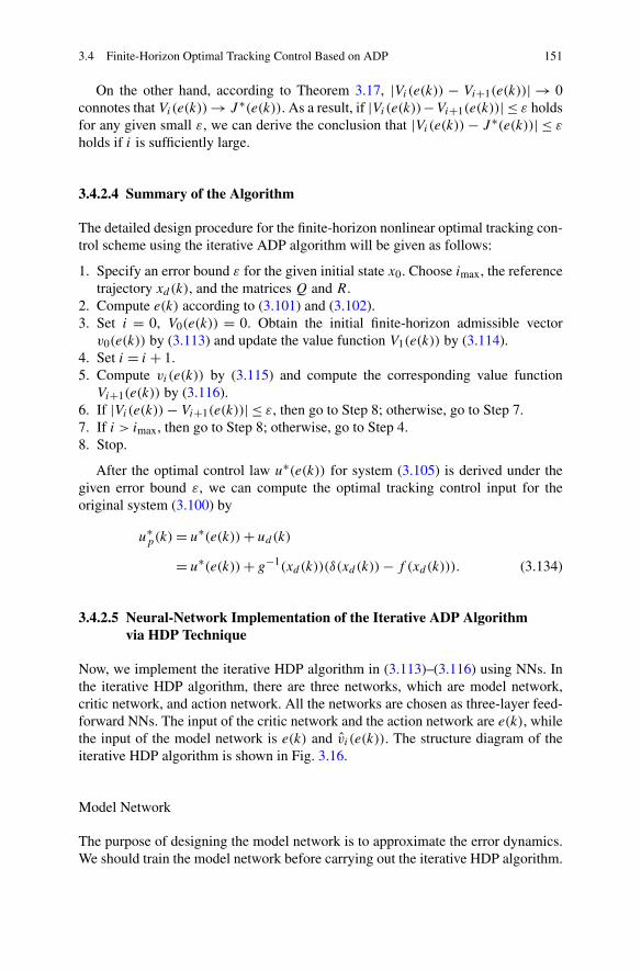
3.4 Finite-Horizon Optimal Tracking Control Based on ADP 151
On the other hand, according to Theorem 3.17, |Vi(e(k)) − Vi+1(e(k))| → 0connotes that Vi(e(k))→ J ∗(e(k)). As a result, if |Vi(e(k))−Vi+1(e(k))| ≤ ε holdsfor any given small ε, we can derive the conclusion that |Vi(e(k))− J ∗(e(k))| ≤ ε
holds if i is sufficiently large.
3.4.2.4 Summary of the Algorithm
The detailed design procedure for the finite-horizon nonlinear optimal tracking con-trol scheme using the iterative ADP algorithm will be given as follows:
1. Specify an error bound ε for the given initial state x0. Choose imax, the referencetrajectory xd(k), and the matrices Q and R.
2. Compute e(k) according to (3.101) and (3.102).3. Set i = 0, V0(e(k)) = 0. Obtain the initial finite-horizon admissible vector
v0(e(k)) by (3.113) and update the value function V1(e(k)) by (3.114).4. Set i = i + 1.5. Compute vi(e(k)) by (3.115) and compute the corresponding value function
Vi+1(e(k)) by (3.116).6. If |Vi(e(k))− Vi+1(e(k))| ≤ ε, then go to Step 8; otherwise, go to Step 7.7. If i > imax, then go to Step 8; otherwise, go to Step 4.8. Stop.
After the optimal control law u∗(e(k)) for system (3.105) is derived under thegiven error bound ε, we can compute the optimal tracking control input for theoriginal system (3.100) by
u∗p(k)= u∗(e(k))+ ud(k)
= u∗(e(k))+ g−1(xd(k))(δ(xd(k))− f (xd(k))). (3.134)
3.4.2.5 Neural-Network Implementation of the Iterative ADP Algorithmvia HDP Technique
Now, we implement the iterative HDP algorithm in (3.113)–(3.116) using NNs. Inthe iterative HDP algorithm, there are three networks, which are model network,critic network, and action network. All the networks are chosen as three-layer feed-forward NNs. The input of the critic network and the action network are e(k), whilethe input of the model network is e(k) and vi (e(k)). The structure diagram of theiterative HDP algorithm is shown in Fig. 3.16.
Model Network
The purpose of designing the model network is to approximate the error dynamics.We should train the model network before carrying out the iterative HDP algorithm.
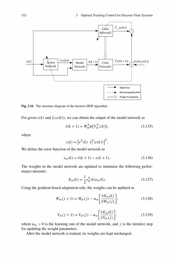
152 3 Optimal Tracking Control for Discrete-Time Systems
Fig. 3.16 The structure diagram of the iterative HDP algorithm
For given e(k) and vi (e(k)), we can obtain the output of the model network as
e(k + 1)=WTmφ
(V Tmz(k)
), (3.135)
where
z(k)= [eT(k) vT
i (e(k))]T.
We define the error function of the model network as
em(k)= e(k + 1)− e(k + 1). (3.136)
The weights in the model network are updated to minimize the following perfor-mance measure:
Em(k)= 1
2eTm(k)em(k). (3.137)
Using the gradient-based adaptation rule, the weights can be updated as
Wm(j + 1)=Wm(j)− αm
[∂Em(k)
∂Wm(j)
], (3.138)
Vm(j + 1)= Vm(j)− αm
[∂Em(k)
∂Vm(j)
], (3.139)
where αm > 0 is the learning rate of the model network, and j is the iterative stepfor updating the weight parameters.
After the model network is trained, its weights are kept unchanged.
3.4 Finite-Horizon Optimal Tracking Control Based on ADP 153
Critic Network
The critic network is used to approximate the value function Vi(e(k)). The outputof the critic network is denoted
Vi(e(k))=WTciφ
(V Tcie(k)
). (3.140)
The target function can be written as
Vi(e(k))= eT(k)Qe(k)+ vTi−1(e(k))Rvi−1(e(k))+ Vi−1(e(k + 1)). (3.141)
Then, we define the error function for the critic network as
eci(k)= Vi (e(k))− Vi(e(k)). (3.142)
The objective function to be minimized for the critic network is
Eci(k)= 1
2eTci(k)eci(k). (3.143)
The weight updating rule for training the critic network is also a gradient-basedadaptation, given by
Wci(j + 1)=Wci(j)− αc
[∂Eci(k)
∂Wci(j)
], (3.144)
Vci(j + 1)= Vci(j)− αc
[∂Eci(k)
∂Vci(j)
], (3.145)
where αc > 0 is the learning rate of the critic network, and j is the inner-loop itera-tive step for updating the weight parameters.
Action Network
In the action network, the state e(k) is used as input to obtain the optimal control.The output can be formulated as
vi (e(k))=WTaiφ
(V Taie(k)
). (3.146)
The target control input is given by
vi(e(k))= −1
2R−1gT(e(k)+ xd(k))
∂Vi(e(k + 1))
∂e(k + 1). (3.147)
The error function of the action network can be defined as
eai(k)= vi (e(k))− vi(e(k)). (3.148)
154 3 Optimal Tracking Control for Discrete-Time Systems
The weights of the action network are updated to minimize the following perfor-mance error measure:
Eai(k)= 1
2eTai(k)eai(k). (3.149)
Similarly, the weight updating algorithm is
Wai(j + 1)=Wai(j)− αa
[∂Eai(k)
∂Wai(j)
], (3.150)
Vai(j + 1)= Vai(j)− αa
[∂Eai(k)
∂Vai(j)
], (3.151)
where αa > 0 is the learning rate of the action network, and j is the inner-loopiterative step for updating the weight parameters.
3.4.3 Simulations
In this part, two simulation examples are provided to confirm the theoretical results.
Example 3.19 The first example is derived from [5] with some modifications. Con-sider the following nonlinear system:
x(k + 1)= f (x(k))+ g(x(k))up(k), (3.152)
where x(k)= [x1(k) x2(k)]T ∈R2 and up(k)= [up1(k) up2(k)]T ∈R
2 are the stateand control variables, respectively. The parameters of the value function are chosenas Q= 0.5I and R = 2I , where I denotes the identity matrix with suitable dimen-sions. The state of the controlled system is initialized by x(0)= [0.8 − 0.5]T. Thesystem functions are given as
f (x(k))=[
sin(0.5x2(k))x21(k)
cos(1.4x2(k)) sin(0.9x1(k))
], g(x(k))=
[1 00 1
].
The reference trajectory for the above system is selected as
xd(k)=[
sin(0.25(k))cos(0.25(k))
].
We set the error bound of the iterative HDP algorithm as ε = 10−5 and im-plement the algorithm at time instant k = 0. The initial control vector of sys-tem (3.105) can be computed as v0(e(0)) = [0.64 sin(0.25) − sin(0.72) cos(0.7)]T,where e(0)= [0.8 −1.5]T. Then, we choose three-layer feedforward NNs as modelnetwork, critic network, and action network with the structures 4–8–2, 2–8–1, 2–8–2, respectively. The initial weights of the three networks are all set to be random
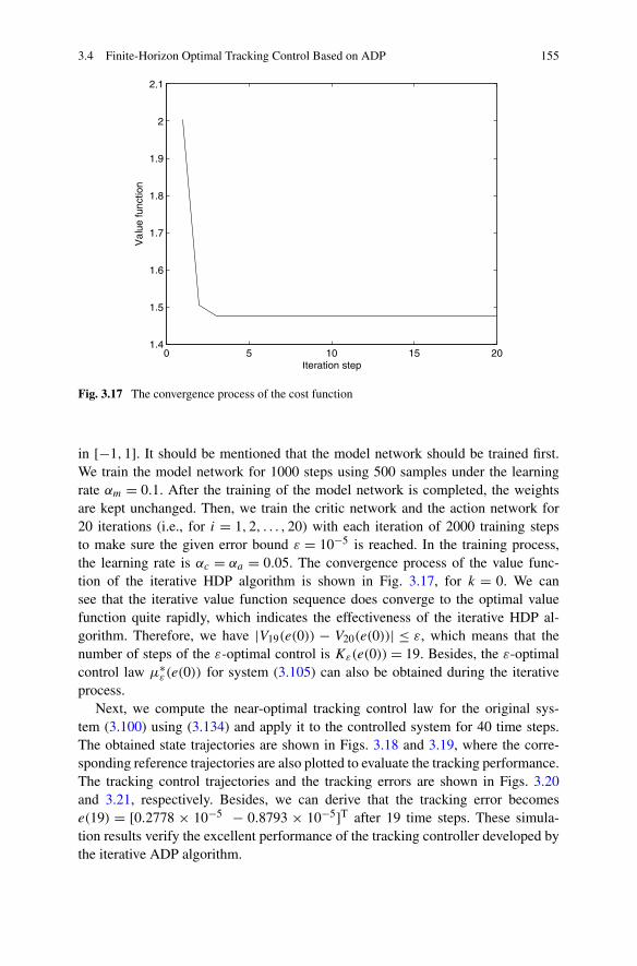
3.4 Finite-Horizon Optimal Tracking Control Based on ADP 155
Fig. 3.17 The convergence process of the cost function
in [−1,1]. It should be mentioned that the model network should be trained first.We train the model network for 1000 steps using 500 samples under the learningrate αm = 0.1. After the training of the model network is completed, the weightsare kept unchanged. Then, we train the critic network and the action network for20 iterations (i.e., for i = 1,2, . . . ,20) with each iteration of 2000 training stepsto make sure the given error bound ε = 10−5 is reached. In the training process,the learning rate is αc = αa = 0.05. The convergence process of the value func-tion of the iterative HDP algorithm is shown in Fig. 3.17, for k = 0. We cansee that the iterative value function sequence does converge to the optimal valuefunction quite rapidly, which indicates the effectiveness of the iterative HDP al-gorithm. Therefore, we have |V19(e(0)) − V20(e(0))| ≤ ε, which means that thenumber of steps of the ε-optimal control is Kε(e(0)) = 19. Besides, the ε-optimalcontrol law μ∗
ε(e(0)) for system (3.105) can also be obtained during the iterativeprocess.
Next, we compute the near-optimal tracking control law for the original sys-tem (3.100) using (3.134) and apply it to the controlled system for 40 time steps.The obtained state trajectories are shown in Figs. 3.18 and 3.19, where the corre-sponding reference trajectories are also plotted to evaluate the tracking performance.The tracking control trajectories and the tracking errors are shown in Figs. 3.20and 3.21, respectively. Besides, we can derive that the tracking error becomese(19) = [0.2778 × 10⁻⁵ − 0.8793 × 10⁻⁵]T after 19 time steps. These simula-tion results verify the excellent performance of the tracking controller developed bythe iterative ADP algorithm.
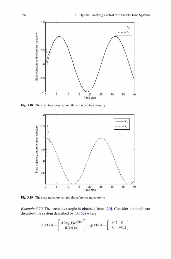
156 3 Optimal Tracking Control for Discrete-Time Systems
Fig. 3.18 The state trajectory x1 and the reference trajectory r1
Fig. 3.19 The state trajectory x2 and the reference trajectory r2
Example 3.20 The second example is obtained from [20]. Consider the nonlineardiscrete-time system described by (3.152) where
f (x(k))=[
0.2x1(k)ex2
2 (k)
0.3x32(k)
], g(x(k))=
[−0.2 00 −0.2
].
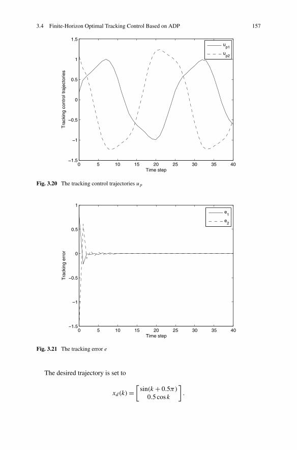
3.4 Finite-Horizon Optimal Tracking Control Based on ADP 157
Fig. 3.20 The tracking control trajectories up
Fig. 3.21 The tracking error e
The desired trajectory is set to
xd(k)=[
sin(k + 0.5π)0.5 cosk
].
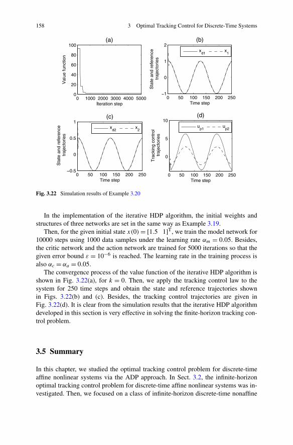
158 3 Optimal Tracking Control for Discrete-Time Systems
Fig. 3.22 Simulation results of Example 3.20
In the implementation of the iterative HDP algorithm, the initial weights andstructures of three networks are set in the same way as Example 3.19.
Then, for the given initial state x(0)= [1.5 1]T, we train the model network for10000 steps using 1000 data samples under the learning rate αm = 0.05. Besides,the critic network and the action network are trained for 5000 iterations so that thegiven error bound ε = 10−6 is reached. The learning rate in the training process isalso αc = αa = 0.05.
The convergence process of the value function of the iterative HDP algorithm isshown in Fig. 3.22(a), for k = 0. Then, we apply the tracking control law to thesystem for 250 time steps and obtain the state and reference trajectories shownin Figs. 3.22(b) and (c). Besides, the tracking control trajectories are given inFig. 3.22(d). It is clear from the simulation results that the iterative HDP algorithmdeveloped in this section is very effective in solving the finite-horizon tracking con-trol problem.
3.5 Summary
In this chapter, we studied the optimal tracking control problem for discrete-timeaffine nonlinear systems via the ADP approach. In Sect. 3.2, the infinite-horizonoptimal tracking control problem for discrete-time affine nonlinear systems was in-vestigated. Then, we focused on a class of infinite-horizon discrete-time nonaffine
References 159
nonlinear systems in Sect. 3.3. In Sect. 3.4, the finite-horizon optimal tracking con-trol problem was studied. Several numerical simulations showed that the presentmethods are effective and can be used for a wide class of nonlinear systems.
References
1. Aganovic Z, Gajic Z (1994) The successive approximation procedure for finite-time optimalcontrol of bilinear systems. IEEE Trans Autom Control 39:1932–1935
2. Cimen T, Banks SP (2004) Nonlinear optimal tracking control with application to super-tankers for autopilot design. Automatica 40:1845–1863
3. Cui LL, Zhang HG, Chen B, Zhang QL (2010) Asymptotic tracking control scheme for me-chanical systems with external disturbances and friction. Neurocomputing 73:1293–1302
4. Devasiad S, Chen D, Paden B (1996) Nonlinear inversion-based output tracking. IEEE TransAutom Control 41:930–942
5. Dierks T, Jagannathan S (2009) Optimal tracking control of affine nonlinear discrete-timesystems with unknown internal dynamics. In: Proceedings of joint 48th IEEE conference ondecision and control and 28th Chinese control conference, Shanghai, China, pp 6750–6755
6. Enns R, Si J (2003) Helicopter trimming and tracking control using direct neural dynamicprogramming. IEEE Trans Neural Netw 14:929–939
7. Gao D, Tang G, Zhang B (2006) Approximate optimal tracking control for a class of nonlinearsystems with disturbances. In: Proceedings of 6th world congress on intelligent control andautomation, Dalian, China, pp 521–525
8. Ha IJ, Gilbert EG (1987) Robust tracking in nonlinear systems. IEEE Trans Autom Control32:763–771
9. Hsu CT, Chen SL (2003) Nonlinear control of a 3-pole active magnetic bearing system. Au-tomatica 39:291–298
10. Lewis FL, Syrmos VL (1995) Optimal control. Wiley, New York11. Mclain TW, Bailry CA, Beard RW (1999) Synthesis and experimental testing of a nonlinear
optimal tracking controller. In: Proceedings of the American control conference, San Diego,CA, USA, pp 2847–2851
12. Park YM, Choi MS, Lee KY (1996) An optimal tracking neuro-controller for nonlinear dy-namic systems. IEEE Trans Neural Netw 7:1009–1110
13. Robbins H, Monro S (1951) A stochastic approximation method. Ann Math Stat 22:400–40714. Si J, Wang YT (2001) On-line learning control by association and reinforcement. IEEE Trans
Neural Netw 12:264–27615. Stefano ML (1981) Optimal design of PID regulators. Int J Control 33:601–61616. Yang Q, Jagannathan S (2007) Online reinforcement learning neural network controller de-
sign for nanomanipulation. In: Proceedings of the IEEE symposium on approximate dynamicprogramming and reinforcement learning, Honolulu, HI, pp 225–232
17. Wang FY, Jin N, Liu D, Wei Q (2011) Adaptive dynamic programming for finite-horizonoptimal control of discrete-time nonlinear systems with ε-error bound. IEEE Trans NeuralNetw 22:24–36
18. Wang D, Liu D, Wei Q (2012) Finite-horizon neuro-optimal tracking control for a class ofdiscrete-time nonlinear systems using adaptive dynamic programming approach. Neurocom-puting 78:14–22
19. Zhang HG, Yang J, Su CY (2007) T-S fuzzy-model-based robust H-infinity design for net-worked control systems with uncertainties. IEEE Trans Ind Inform 3:289–301
20. Zhang HG, Wei QL, Luo YH (2008) A novel infinite-time optimal tracking control schemefor a class of discrete-time nonlinear systems via the greedy HDP iteration algorithm. IEEETrans Syst Man Cybern, Part B, Cybern 38:937–942
160 3 Optimal Tracking Control for Discrete-Time Systems
21. Zhang HG, Wang ZS, Liu DR (2009) Global asymptotic stability and robust stability of a classof Cohen–Grossberg neural networks with mixed delays. IEEE Trans Circuits Syst I, RegulPap 56:616–629
22. Zheng CD, Zhang HG (2007) Generalized multivariate rectangular matrix Pade-type approx-imants. IEEE Trans Circuits Syst I, Regul Pap 54:2099–2105
23. Zheng CD, Zhang HG, Tian H (2007) Generalized homogeneous multivariate matrix Pade-type approximants and Pade approximants. IEEE Trans Autom Control 52:2160–2165
24. Zheng CD, Zhang HG, Wang ZS (2009) Delay-dependent globally exponential stability crite-ria for static neural networks: an LMI approach. IEEE Trans Neural Netw 56:605–609
Chapter 4Optimal State Feedback Control of NonlinearSystems with Time Delays
4.1 Introduction
For time-delay system, much research is about decentralized control, synchroniza-tion control, and stability analysis [4–7, 10–13, 15, 16]. However, the optimal con-trol problem is often encountered in industrial production. So in this chapter, the op-timal state feedback control problems of nonlinear systems with time delays will bediscussed. In general, the optimal control for the time-delay systems is an infinite-dimensional control problem [1], which is very difficult to solve. The analysis ofsystems with time delays is much more difficult than that of systems without de-lays, and there is no method strictly facing this problem for nonlinear time-delaysystems.
In Sect. 4.2, the optimal state feedback control problem of nonlinear systemswith time delays both in states and controls is solved. By introducing a delay ma-trix function, we can obtain the explicit expression of the optimal control function.Also, it is proved that the value function converges to the optimum using the presentiterative ADP algorithm.
In Sect. 4.3, we study the optimal control problem of nonlinear time-delaysystems with saturating actuators. First, the HJB equation for time-delay sys-tems with saturating actuators is derived using a nonquadratic function. In or-der to solve this HJB equation, two optimization searching processes are de-veloped. We also give the convergence proof for the new iterative HDP algo-rithm. Finally, two neural networks are used to implement the iterative HDP al-gorithm.
The above two sections are for the infinite-horizon optimal control problem. Tothe best of our knowledge, only [8] presented finite-horizon optimal control in detail.However, time-delay nonlinear systems have not been considered. So, we developan effective algorithm to solve the finite-horizon optimal control problem for a classof time-delay systems in Sect. 4.4.
H. Zhang et al., Adaptive Dynamic Programming for Control,Communications and Control Engineering, DOI 10.1007/978-1-4471-4757-2_4,© Springer-Verlag London 2013
161
162 4 Optimal State Feedback Control of Nonlinear Systems with Time Delays
4.2 Infinite-Horizon Optimal State Feedback Control via DelayMatrix
4.2.1 Problem Formulation
We consider the following discrete-time affine nonlinear system with time delays instate and control variables:
x(k + 1)= f (x(k), x(k − σ))+ g0(x(k), x(k − σ))u(k)
+ g1(x(k), x(k − σ))u(k − τ), (4.1)
with the initial condition given by x(s) = φ(s), s = −σ,−σ + 1, . . . ,0, wherex(k) ∈ R
n is the state vector, f : Rn × Rn → R
n, and g0, g1 : Rn × Rn → R
n×m
are differentiable functions and we have the control u(k) ∈ Rm. The state and con-
trol delays σ and τ are both nonnegative integers. Assume that f (x(k), x(k−σ))+g0(x(k), x(k − σ))u(k)+ g1(x(k), x(k − σ))u(k − τ) is Lipschitz continuous on aset Ω in R
n containing the origin, and that the system (4.1) is controllable in thesense that there exists a bounded control on Ω that asymptotically stabilizes thesystem. In this section, we mainly discuss how to design an optimal state feedbackcontroller for this class of delayed discrete-time systems. Therefore, we desire tofind the optimal control u(x) satisfying u(x(k))= u(k) to minimize the generalizedcost functional as follows:
J (x(0), u)=∞∑
k=0
{xT(k)Q0x(k)+ 2xT(k)Q1x(k − σ)
+ xT(k − σ)Q2x(k − σ)+ uT(k)R0u(k)
+ 2uT(k)R1u(k − τ)+ uT(k − τ)R2u(k − τ)}, (4.2)
where[Q0 Q1
QT1 Q2
] ≥ 0 and[ R0 R1
RT1 R2
]> 0 and l(x(k), x(k − σ),u(k), u(k − τ)) =
xT(k)Q0x(k) + 2xT(k)Q1x(k − σ) + xT(k − σ)Q2x(k − σ) + uT(k)R0u(k) +2uT(k)R1u(k − τ)+ uT(k − τ)R2u(k − τ) is the utility function. Let J ∗(x) denotethe optimal value function which satisfies
J ∗(x)= minu
J (x,u). (4.3)
According to Bellman’s optimality principle, we get the following HJB equation:
J ∗(x(k))= minu(k)
{xT(k)Q0x(k)+ 2xT(k)Q1x(k − σ)
+ xT(k − σ)Q2x(k − σ)+ uT(k)R0u(k)
+ 2uT(k)R1u(k − τ)+uT(k − τ)R2u(k − τ)
+ J ∗(x(k + 1))}. (4.4)
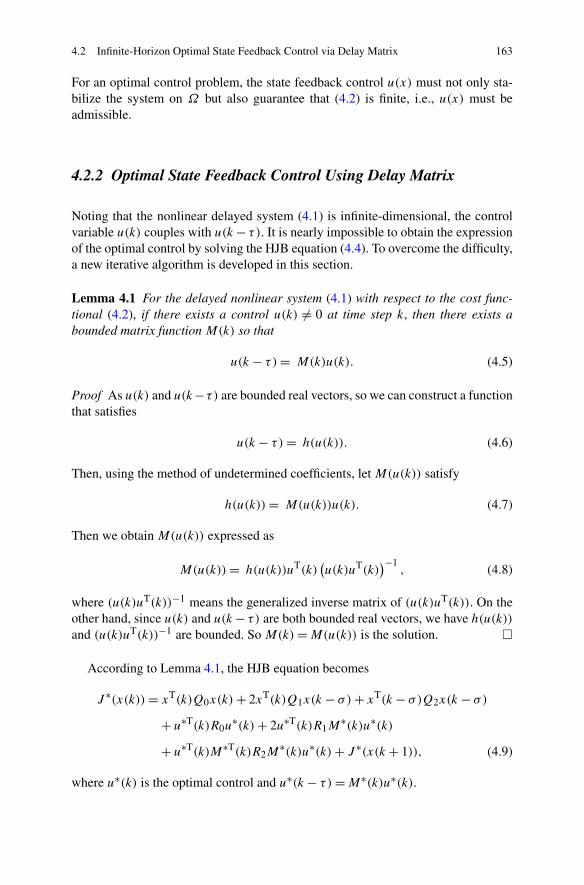
4.2 Infinite-Horizon Optimal State Feedback Control via Delay Matrix 163
For an optimal control problem, the state feedback control u(x) must not only sta-bilize the system on Ω but also guarantee that (4.2) is finite, i.e., u(x) must beadmissible.
4.2.2 Optimal State Feedback Control Using Delay Matrix
Noting that the nonlinear delayed system (4.1) is infinite-dimensional, the controlvariable u(k) couples with u(k− τ). It is nearly impossible to obtain the expressionof the optimal control by solving the HJB equation (4.4). To overcome the difficulty,a new iterative algorithm is developed in this section.
Lemma 4.1 For the delayed nonlinear system (4.1) with respect to the cost func-tional (4.2), if there exists a control u(k) �= 0 at time step k, then there exists abounded matrix function M(k) so that
u(k − τ)= M(k)u(k). (4.5)
Proof As u(k) and u(k−τ) are bounded real vectors, so we can construct a functionthat satisfies
u(k − τ)= h(u(k)). (4.6)
Then, using the method of undetermined coefficients, let M(u(k)) satisfy
h(u(k))= M(u(k))u(k). (4.7)
Then we obtain M(u(k)) expressed as
M(u(k))= h(u(k))uT(k)(u(k)uT(k)
)−1, (4.8)
where (u(k)uT(k))−1 means the generalized inverse matrix of (u(k)uT(k)). On theother hand, since u(k) and u(k− τ) are both bounded real vectors, we have h(u(k))and (u(k)uT(k))−1 are bounded. So M(k)=M(u(k)) is the solution. �
According to Lemma 4.1, the HJB equation becomes
J ∗(x(k))= xT(k)Q0x(k)+ 2xT(k)Q1x(k − σ)+ xT(k − σ)Q2x(k − σ)
+ u∗T(k)R0u∗(k)+ 2u∗T(k)R1M
∗(k)u∗(k)
+ u∗T(k)M∗T(k)R2M∗(k)u∗(k)+ J ∗(x(k + 1)), (4.9)
where u∗(k) is the optimal control and u∗(k − τ)=M∗(k)u∗(k).
164 4 Optimal State Feedback Control of Nonlinear Systems with Time Delays
According to Bellman’s principle of optimality, we can obtain the optimal controlby differentiating the HJB equation (4.9) with respect to the control u. Then weobtain the optimal control u∗(k) formulated as
u∗(k)= − 1
2
(R0 + 2R1M
∗(k)+M∗T(k)R2M∗(k)
)−1
× (g0 (x(k), x(k − σ))+ g1 (x(k), x(k − σ))M∗(k)
)T
× ∂J ∗(x(k + 1))
∂x(k + 1). (4.10)
In (4.10), the inverse of(R0 + 2R1M
∗(k)+M∗T(k)R2M∗(k)
)should exist.
From (4.10), the explicit optimal control expression u∗ is obtained by solving theHJB equation (4.9). We see that the optimal control u∗ depends on M∗ and J ∗(x),where J ∗(x) is a solution of the HJB equation (4.9). It is still an open question howto solve the HJB equation and there is currently no method for rigorously seeking forthe value function of this delayed optimal control problem. Furthermore, the optimaldelay matrix function M∗ is also unknown, which makes the optimal control u∗more difficult to obtain. So an iterative index i is introduced into the ADP approachto obtain the optimal control iteratively.
First, for i = 0,1, . . . , let
u[i+1](k − τ)= M [i](k)u[i+1](k), (4.11)
where M [0](k)= I and u[0](k − τ)=M [0](k)u[0](k). We start with an initial valuefunction V [0](x(k))= 0, and the control u[0](k) can be computed as follows:
u[0](x(k))= arg minu
{Γ [0] + V [0](x(k + 1))
}, (4.12)
where
Γ [0] = xT(k)Q0x(k)+ 2xT(k)Q1x(k − σ)
+ xT(k − σ)Q2x(k − σ)+ u[0]T(k)R0u[0](k)
+ 2u[0]T(k)R1M[0](k)u[0](k)
+ u[0]T(k)M [0]T(k)R2M[0](k)u[0](k).
Then, the value function is updated as
V [1](x(k))= Γ [0] + V [0](x(k + 1)). (4.13)
Thus, for i = 1,2, . . . , the iterative ADP can be used to implement the iterationbetween
u[i](x(k))= arg minu
{Γ [i] + V [i](x(k + 1))
}
4.2 Infinite-Horizon Optimal State Feedback Control via Delay Matrix 165
= − 1
2
(R0 + 2R1M
[i−1](k)+M [i−1]T(k)R2M[i−1](k)
)−1
×(g0(x(k), x(k − σ))+ g1 (x(k), x(k − σ))M [i−1](k)
)T
× ∂V [i](x(k + 1))
∂x(k + 1), (4.14)
where
Γ [i] = xT(k)Q0x(k)+ 2xT(k)Q1x(k − σ)
+ xT(k − σ)Q2x(k − σ)+ u[i]T(k)R0u[i](k)
+ 2u[i]T(k)R1M[i−1](k)u[i](k)
+ u[i]T(k)M [i−1]T(k)R2M[i−1](k)u[i](k),
and
V [i+1](x(k))= Γ [i] + V [i](x(k + 1)). (4.15)
From (4.14) and (4.15), it can be seen that, during the iterative process, the con-trol actions for different control steps obey different control laws. After iteration i,the obtained control law sequence is (u[0], u[1], . . . , u[i]). For the infinite-horizonproblem, both the optimal value function and the optimal control law are unique.Therefore, it is necessary to show that the iterative value function V [i](x(k)) willconverge when iteration i → ∞ under the iterative control u[i](k) and this will beproved in the following.
Lemma 4.2 Let u[i](k), k = 0,1 . . . be any sequence of control, and let u[i](k) beexpressed as (4.14). Define V [i+1](x(k)) as (4.15) and Λ[i+1](x(k)) as
Λ[i+1](x(k))= xT(k)Q0x(k)+ 2xT(k)Q1x(k − σ)
+ xT(k − σ)Q2x(k − σ)+ u[i]T(k)R0u[i](k)
+ 2u[i]T(k)R1M[i−1](k)u[i](k)
+ u[i]T(k)M [i−1]T(k)R2M[i−1](k)u[i](k)
+Λ[i](x(k + 1)). (4.16)
If V [0](x(k))=Λ[0](x(k))= 0, then V [i](x(k))≤Λ[i](x(k)), ∀i.
In order to prove the convergence of the value function, the following theorem isalso necessary.
Theorem 4.3 (cf. [9]) Let the value function V [i](x(k)) be defined by (4.15). Ifx(k) of the system (4.1) is controllable, then there exists an upper bound Y suchthat 0 ≤ V [i](x(k))≤ Y , ∀i.
166 4 Optimal State Feedback Control of Nonlinear Systems with Time Delays
Proof As the system (4.1) is Lipschitz, M [i](k) is a bounded matrix for i = 0,1, . . . .Define a delay matrix function M(k) which enforces
χT (R0 + 2R1M(k)+ MT(k)R2M(k))χ
− χT(R0 + 2R1M
[i](k)+M [i]T(k)R2M[i](k)
)χ ≥ 0 (4.17)
for ∀i, where χ is any nonzero m-dimensional vector. Let u(k), k = 0,1 . . . be anyadmissible control input. Define a new sequence P [i](x(k)) as follows:
P [i+1](x(k))= xT(k)Q0x(k)+ 2xT(k)Q1x(k − σ)
+ xT(k − σ)Q2x(k − σ)+ uT(k)R0u(k)
+ 2uT(k)R1M(k)u(k)
+ uT(k)MT(k)R2M(k)u(k)+P [i](x(k + 1)), (4.18)
where we let P [0](x(k))= V [0](x(k))= 0 and u(k − τ)= M(k)u(k). V [i](x(k)) isupdated by (4.15). Thus, we obtain
P [i+1](x(k))−P [i](x(k)) = P [i](x(k + 1))−P [i−1](x(k + 1))
...
= P [1](x(k + i))−P [0](x(k + i)).
(4.19)
Because P [0](x(k + i))= 0, we have
P [i+1](x(k))= P [1](x(k + i))+ P [i](x(k))
=i∑
j=0
P [1](x(k + j)). (4.20)
According to (4.18), (4.20) can be rewritten as
P [i+1](x(k))=i∑
j=0
Ξ(k + j)≤∞∑
j=0
Ξ(k + j), (4.21)
where
Ξ(k + j)= xT(k + j)Q0x(k + j)+ 2xT(k + j)Q1x(k + j − σ)
+ xT(k + j − σ)Q2x(k + j − σ)+ uT(k + j)R0u(k + j)
+ 2uT(k + j)R1M(k + j)u(k + j)
+ uT(k + j)MT(k + j)R2M(k + j)u(k + j).
4.2 Infinite-Horizon Optimal State Feedback Control via Delay Matrix 167
Noting that the control input u(k), k = 0,1, . . . , is an admissible control, we obtain
∀i : P [i+1](x(k))≤∞∑j=0
P [i+j ](x(k + j))≤Y. (4.22)
From Lemma 4.1, we have
∀i : V [i+1](x(k))≤ P [i+1](x(k))≤Y. (4.23)
This completes the proof. �
With Lemma 4.1 and Theorem 4.3, the following main theorem can be derived.
Theorem 4.4 Define the value function V [i](x(k)) as (4.15), with V [0](x(k)) = 0.If x(k) for the system (4.1) is controllable, then V [i](x(k)) is a nondecreasingsequence satisfying V [i](x(k)) ≤ V [i+1](x(k)), and V [i](x(k)) is convergent asi → ∞.
Proof For convenience in our analysis, define a new sequenceΦ[i](x(k)) as follows:
Φ[i+1](x(k))=xT(k)Q0x(k)+ 2xT(k)Q1x(k − σ)
+xT(k−σ)Q2x(k−σ)+u[i+1]T(k)R0u[i+1](k)
+ 2u[i+1]T(k)R1M(i)(k)u[i+1](k)
+ u[i+1]T(k)M [i]T(k)R2M[i](k)u[i+1](k)
+Φ[i](x(k + 1)), (4.24)
where u[i](k) is obtained by (4.14) and Φ[0](x(k))= V [0](x(k))= 0.In the following part, we prove Φ[i](x(k)) ≤ V [i+1](x(k)) by mathematical in-
duction.First, we prove that it holds for i = 0. Noting that
V [1](x(k))−Φ[0](x(k))= xT(k)Q0x(k)+ 2xT(k)Q1x(k − σ)
+ xT(k − σ)Q2x(k − σ)
≥ 0, (4.25)
for i = 0, we get
V [1](x(k))≥Φ[0](x(k)). (4.26)
Second, we assume it holds for i − 1, i.e., V [i](x(k))−Φ[i−1](x(k))≥ 0, ∀x(k).Then, for i, from (4.15) and (4.24), we obtain
V [i+1](x(k))−Φ[i](x(k))= V [i](x(k + 1))−Φ[i−1](x(k + 1))
≥ 0, (4.27)
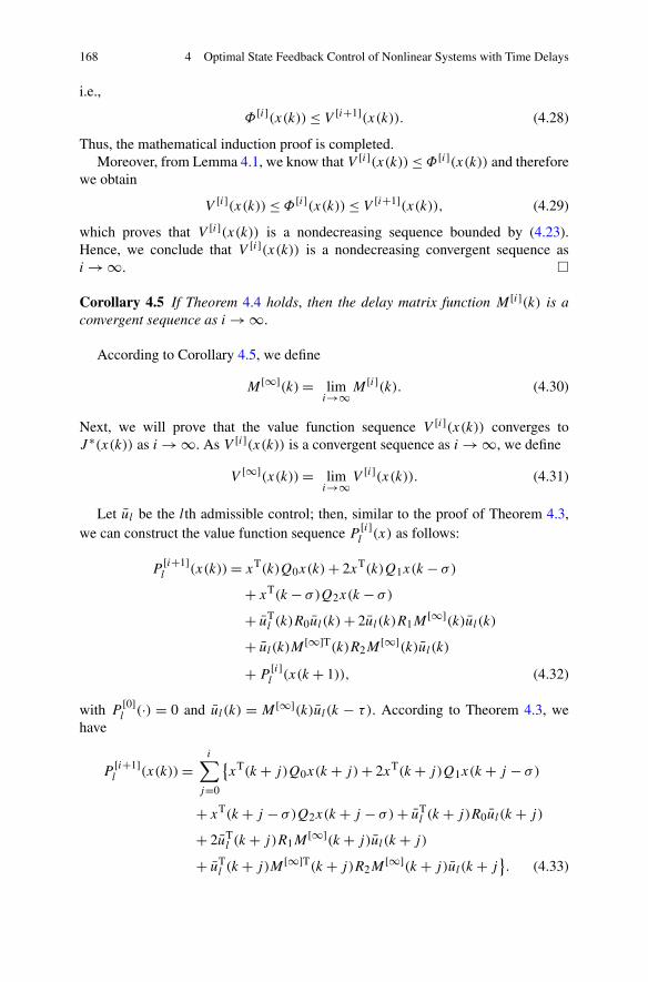
168 4 Optimal State Feedback Control of Nonlinear Systems with Time Delays
i.e.,
Φ[i](x(k))≤ V [i+1](x(k)). (4.28)
Thus, the mathematical induction proof is completed.Moreover, from Lemma 4.1, we know that V [i](x(k))≤Φ[i](x(k)) and therefore
we obtain
V [i](x(k))≤Φ[i](x(k))≤ V [i+1](x(k)), (4.29)
which proves that V [i](x(k)) is a nondecreasing sequence bounded by (4.23).Hence, we conclude that V [i](x(k)) is a nondecreasing convergent sequence asi → ∞. �
Corollary 4.5 If Theorem 4.4 holds, then the delay matrix function M [i](k) is aconvergent sequence as i → ∞.
According to Corollary 4.5, we define
M [∞](k)= limi→∞M [i](k). (4.30)
Next, we will prove that the value function sequence V [i](x(k)) converges toJ ∗(x(k)) as i → ∞. As V [i](x(k)) is a convergent sequence as i → ∞, we define
V [∞](x(k))= limi→∞V [i](x(k)). (4.31)
Let ul be the lth admissible control; then, similar to the proof of Theorem 4.3,we can construct the value function sequence P [i]
l (x) as follows:
P[i+1]l (x(k))= xT(k)Q0x(k)+ 2xT(k)Q1x(k − σ)
+ xT(k − σ)Q2x(k − σ)
+ uTl (k)R0ul(k)+ 2ul(k)R1M
[∞](k)ul(k)
+ ul(k)M[∞]T(k)R2M
[∞](k)ul(k)
+ P[i]l (x(k + 1)), (4.32)
with P[0]l (·) = 0 and ul(k) = M [∞](k)ul(k − τ). According to Theorem 4.3, we
have
P[i+1]l (x(k))=
i∑
j=0
{xT(k + j)Q0x(k + j)+ 2xT(k + j)Q1x(k + j − σ)
+ xT(k + j − σ)Q2x(k + j − σ)+ uTl (k + j)R0ul(k + j)
+ 2uTl (k + j)R1M
[∞](k + j)ul(k + j)
+ uTl (k + j)M [∞]T(k + j)R2M
[∞](k + j)ul(k + j}. (4.33)
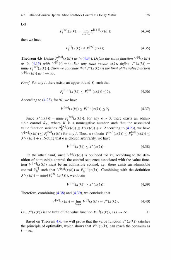
4.2 Infinite-Horizon Optimal State Feedback Control via Delay Matrix 169
Let
P[∞]l (x(k))= lim
i→∞P[i+1]l (x(k)); (4.34)
then we have
P[i]l (x(k))≤ P
[∞]l (x(k)). (4.35)
Theorem 4.6 Define P [∞]l (x(k)) as in (4.34). Define the value function V [i](x(k))
as in (4.15) with V [0](·) = 0. For any state vector x(k), define J ∗(x(k)) =minl{P [∞]
l (x(k))}. Then we conclude that J ∗(x(k)) is the limit of the value functionV [i](x(k)) as i → ∞.
Proof For any l, there exists an upper bound Yl such that
P[i+1]l (x(k))≤ P
[∞]l (x(k))≤ Yl. (4.36)
According to (4.23), for ∀l, we have
V [∞](x(k))≤ P[∞]l (x(k))≤ Yl. (4.37)
Since J ∗(x(k)) = minl{P [∞]l (x(k))}, for any ε > 0, there exists an admis-
sible control uK , where K is a nonnegative number such that the associatedvalue function satisfies P [∞]
K (x(k)) ≤ J ∗(x(k)) + ε. According to (4.23), we have
V [∞](x(k)) ≤ P[∞]l (x(k)) for any l. Thus, we obtain V [∞](x(k)) ≤ P
[∞]K (x(k)) ≤
J ∗(x(k))+ ε. Noting that ε is chosen arbitrarily, we have
V [∞](x(k))≤ J ∗(x(k)). (4.38)
On the other hand, since V [i](x(k)) is bounded for ∀i, according to the defi-nition of admissible control, the control sequence associated with the value func-tion V [∞](x(k)) must be an admissible control, i.e., there exists an admissible
control u[i]N such that V [∞](x(k)) = P
[∞]N (x(k)). Combining with the definition
J ∗(x(k))= minl{P [∞]l (x(k))}, we obtain
V [∞](x(k))≥ J ∗(x(k)). (4.39)
Therefore, combining (4.38) and (4.39), we conclude that
V [∞](x(k))= limi→∞V [i](x(k))= J ∗(x(k)), (4.40)
i.e., J ∗(x(k)) is the limit of the value function V [i](x(k)), as i → ∞. �
Based on Theorem 4.6, we will prove that the value function J ∗(x(k)) satisfiesthe principle of optimality, which shows that V [i](x(k)) can reach the optimum asi → ∞.
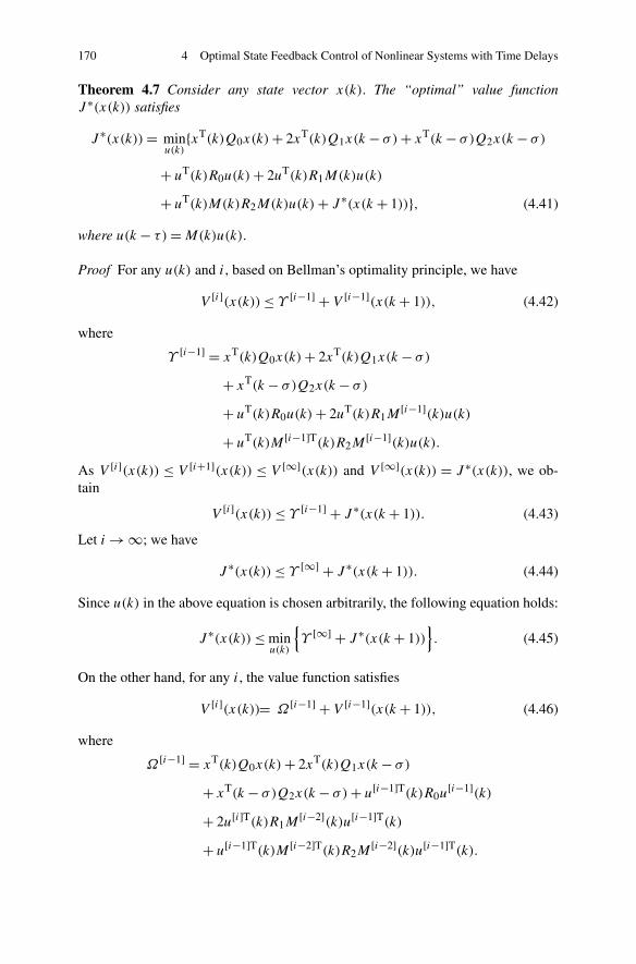
170 4 Optimal State Feedback Control of Nonlinear Systems with Time Delays
Theorem 4.7 Consider any state vector x(k). The “optimal” value functionJ ∗(x(k)) satisfies
J ∗(x(k))= minu(k)
{xT(k)Q0x(k)+ 2xT(k)Q1x(k − σ)+ xT(k − σ)Q2x(k − σ)
+ uT(k)R0u(k)+ 2uT(k)R1M(k)u(k)
+ uT(k)M(k)R2M(k)u(k)+ J ∗(x(k + 1))}, (4.41)
where u(k − τ)=M(k)u(k).
Proof For any u(k) and i, based on Bellman’s optimality principle, we have
V [i](x(k))≤ Υ [i−1] + V [i−1](x(k + 1)), (4.42)
where
Υ [i−1] = xT(k)Q0x(k)+ 2xT(k)Q1x(k − σ)
+ xT(k − σ)Q2x(k − σ)
+ uT(k)R0u(k)+ 2uT(k)R1M[i−1](k)u(k)
+ uT(k)M [i−1]T(k)R2M[i−1](k)u(k).
As V [i](x(k)) ≤ V [i+1](x(k)) ≤ V [∞](x(k)) and V [∞](x(k)) = J ∗(x(k)), we ob-tain
V [i](x(k))≤ Υ [i−1] + J ∗(x(k + 1)). (4.43)
Let i → ∞; we have
J ∗(x(k))≤ Υ [∞] + J ∗(x(k + 1)). (4.44)
Since u(k) in the above equation is chosen arbitrarily, the following equation holds:
J ∗(x(k))≤ minu(k)
{Υ [∞] + J ∗(x(k + 1))
}. (4.45)
On the other hand, for any i, the value function satisfies
V [i](x(k))= Ω [i−1] + V [i−1](x(k + 1)), (4.46)
where
Ω [i−1] = xT(k)Q0x(k)+ 2xT(k)Q1x(k − σ)
+ xT(k − σ)Q2x(k − σ)+ u[i−1]T(k)R0u[i−1](k)
+ 2u[i]T(k)R1M[i−2](k)u[i−1]T(k)
+ u[i−1]T(k)M [i−2]T(k)R2M[i−2](k)u[i−1]T(k).
4.2 Infinite-Horizon Optimal State Feedback Control via Delay Matrix 171
Combining with V [i](x(k))≤ J ∗(x(k)),∀i, we have
J ∗(x(k))≥Ω [i−1] + V [i−1](x(k + 1)). (4.47)
Let i → ∞; then
J ∗(x(k))≥ limi→∞
{Ω [i−1] + V [i−1](x(k + 1))
}
≥ minu(k)
{Ω [∞] + J ∗(x(k + 1))
}. (4.48)
Combining (4.45) with (4.48), we have
J ∗(x(k))= minu(k)
{Ω [∞] + J ∗(x(k + 1))}
= xT(k)Q0x(k)+ 2xT(k)Q1x(k − σ)
+ xT(k − σ)Q2x(k − σ)+ u∗T(k)R0u∗(k)
+ 2u∗T(k)R1M[∞](k)u∗(k)
+ u∗T(k)M [∞]T(k)R2M[∞](k)u∗(k)
+ J ∗(x(k + 1)). (4.49)
Thus, we have u[i](k) → u∗(k) as i → ∞. So does u[i](k − τ). On the other hand,we also have M [i](k)→M [∞](k) and u[i](k − τ)=M [i−1](k)u[i](k). Let i → ∞,and we get
u∗(k − τ)= M [∞](k)u∗(k). (4.50)
Therefore, we have M [∞](k)=M∗(k), and (4.49) can be written as
J ∗(x(k))= xT(k)Q0x(k)+ 2xT(k)Q1x(k − σ)
+ xT(k − σ)Q2x(k − σ)+ u∗T(k)R0u∗(k)
+ 2u∗T(k)R1M∗(k)u∗(k)
+ u∗T(k)M∗T(k)R2M∗(k)u∗(k)
+ J ∗(x(k + 1)), (4.51)
where u∗(k − τ)=M∗(k)u∗(k). �
Therefore, we conclude that the value function V [i](x(k)) converges to the opti-mum J ∗(x(k)) as i → ∞.
In the case of linear systems, the value function is quadratic and the control law islinear. In the nonlinear case, this is not necessarily true and therefore we use neuralnetworks to approximate u[i](k) and V [i](x(k)).
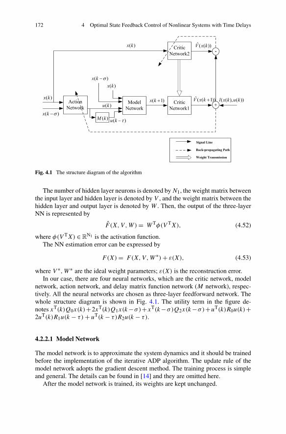
172 4 Optimal State Feedback Control of Nonlinear Systems with Time Delays
Fig. 4.1 The structure diagram of the algorithm
The number of hidden layer neurons is denoted by N1, the weight matrix betweenthe input layer and hidden layer is denoted by V , and the weight matrix between thehidden layer and output layer is denoted by W . Then, the output of the three-layerNN is represented by
F (X,V,W)= WTφ(V TX), (4.52)
where φ(V TX) ∈RN1 is the activation function.
The NN estimation error can be expressed by
F(X)= F(X,V,W ∗)+ ε(X), (4.53)
where V ∗,W ∗ are the ideal weight parameters; ε(X) is the reconstruction error.In our case, there are four neural networks, which are the critic network, model
network, action network, and delay matrix function network (M network), respec-tively. All the neural networks are chosen as three-layer feedforward network. Thewhole structure diagram is shown in Fig. 4.1. The utility term in the figure de-notes xT(k)Q0x(k)+2xT(k)Q1x(k−σ)+xT(k−σ)Q2x(k−σ)+uT(k)R0u(k)+2uT(k)R1u(k − τ)+ uT(k − τ)R2u(k − τ).
4.2.2.1 Model Network
The model network is to approximate the system dynamics and it should be trainedbefore the implementation of the iterative ADP algorithm. The update rule of themodel network adopts the gradient descent method. The training process is simpleand general. The details can be found in [14] and they are omitted here.
After the model network is trained, its weights are kept unchanged.
4.2 Infinite-Horizon Optimal State Feedback Control via Delay Matrix 173
4.2.2.2 The M Network
The M network is to approximate the delay matrix function M(k). The output ofthe M network is denoted
u(k − τ)= WTMφ(V
TMu(k)). (4.54)
We define the error function of the model network as
eM(k)= u(k − τ)− u(k − τ). (4.55)
Define the error measure as
EM(k)= 1
2eTM(k)eM(k). (4.56)
Then, the gradient-based weight updating rule for the M network can be de-scribed by
wM(k + 1)= wM(k)+ΔwM(k), (4.57)
ΔwM(k)= αM
[−∂EM(k)
∂wM(k)
], (4.58)
where αM is the learning rate of the M network.
4.2.2.3 Critic Network
The critic network is used to approximate the value function V [i](x(k)). The outputof the critic network is denoted
V [i](x(k))= WTciφ(V
Tciz(k)). (4.59)
The target function can be written as
V [i+1](x(k))= Γ [i] + V [i](x(k + 1)). (4.60)
Then, we define the error function for the critic network as
eci(k)= V [i+1](x(k))− V [i+1](x(k)). (4.61)
The objective function to be minimized in the critic network is
Eci(k)= 1
2eTci(k)eci(k). (4.62)
So the gradient-based weight updating rule for the critic network is given by
wc(i+1)(k)= wci(k)+Δwci(k), (4.63)
174 4 Optimal State Feedback Control of Nonlinear Systems with Time Delays
Δwci(k)= αc
[−∂Eci(k)
∂wci(k)
], (4.64)
∂Eci(k)
∂wci(k)= ∂Eci(k)
∂V [i](x(k))∂V [i](x(k))∂wci(k)
, (4.65)
where αc > 0 is the learning rate of critic network and wc(k) is the weight vector inthe critic network.
4.2.2.4 Action Network
In the action network, the state x(k) is used as input to create the optimal control.The output can be formulated as
u[i](k)= WTaiφ(V
Taix(k)). (4.66)
And the output target of the action network is given by (4.14). So we define theoutput error of the action network as
eai(k)= u[i](k)− u[i](k), (4.67)
where u[i](k) is the target function which can be described by
u[i](k)= − 1
2
(R0+2R1M
[i−1](k)+M [i−1]T(k)R2M[i−1](k)
)−1
×(g0 (x(k), x(k − σ))+ g1 (x(k), x(k − σ))M [i−1](k)
)T
× ∂V [i](x(k + 1))
∂x(k + 1).
As u[i](k − τ) = M [i−1](k)u[i](k), we have∂u[i](k − τ)
∂u[i](k)= M [i−1](k). Then, ac-
cording to (4.54), M [i−1](k) can be expressed as
M[i−1]ij (k)= V T
Mi
[1 − (
φ(V TMu(k))
)2i
]WMj (4.68)
for i, j = 1,2, . . . ,m. M [i−1]ij (k) denotes the element of row i, column j of ma-
trix M [i−1](k). VMi and WMj mean the column i and column j of the weightmatrices VM and WM , respectively. (φ(V T
Mu(k)))i is the ith element of the vectorφ(V T
Mu(k)).The weights in the action network are updated to minimize the following error
measure:
Eai(k)= 1
2eTai(k)eai(k). (4.69)
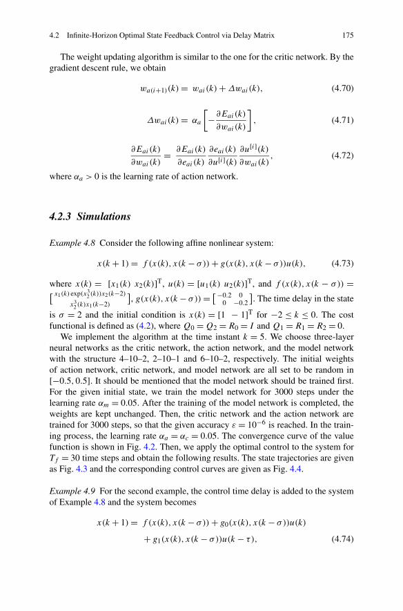
4.2 Infinite-Horizon Optimal State Feedback Control via Delay Matrix 175
The weight updating algorithm is similar to the one for the critic network. By thegradient descent rule, we obtain
wa(i+1)(k)= wai(k)+Δwai(k), (4.70)
Δwai(k)= αa
[−∂Eai(k)
∂wai(k)
], (4.71)
∂Eai(k)
∂wai(k)= ∂Eai(k)
∂eai(k)
∂eai(k)
∂u[i](k)∂u[i](k)∂wai(k)
, (4.72)
where αa > 0 is the learning rate of action network.
4.2.3 Simulations
Example 4.8 Consider the following affine nonlinear system:
x(k + 1)= f (x(k), x(k − σ))+ g(x(k), x(k − σ))u(k), (4.73)
where x(k) = [x1(k) x2(k)]T, u(k) = [u1(k) u2(k)]T, and f (x(k), x(k − σ)) =[ x1(k) exp(x3
2 (k))x2(k−2)
x32 (k)x1(k−2)
], g(x(k), x(k− σ))= [−0.2 0
0 −0.2
]. The time delay in the state
is σ = 2 and the initial condition is x(k) = [1 − 1]T for −2 ≤ k ≤ 0. The costfunctional is defined as (4.2), where Q0 =Q2 =R0 = I and Q1 =R1 =R2 = 0.
We implement the algorithm at the time instant k = 5. We choose three-layerneural networks as the critic network, the action network, and the model networkwith the structure 4–10–2, 2–10–1 and 6–10–2, respectively. The initial weightsof action network, critic network, and model network are all set to be random in[−0.5,0.5]. It should be mentioned that the model network should be trained first.For the given initial state, we train the model network for 3000 steps under thelearning rate αm = 0.05. After the training of the model network is completed, theweights are kept unchanged. Then, the critic network and the action network aretrained for 3000 steps, so that the given accuracy ε = 10−6 is reached. In the train-ing process, the learning rate αa = αc = 0.05. The convergence curve of the valuefunction is shown in Fig. 4.2. Then, we apply the optimal control to the system forTf = 30 time steps and obtain the following results. The state trajectories are givenas Fig. 4.3 and the corresponding control curves are given as Fig. 4.4.
Example 4.9 For the second example, the control time delay is added to the systemof Example 4.8 and the system becomes
x(k + 1)= f (x(k), x(k − σ))+ g0(x(k), x(k − σ))u(k)
+ g1(x(k), x(k − σ))u(k − τ), (4.74)
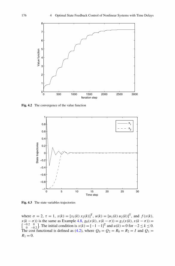
176 4 Optimal State Feedback Control of Nonlinear Systems with Time Delays
Fig. 4.2 The convergence of the value function
Fig. 4.3 The state variables trajectories
where σ = 2, τ = 1, x(k) = [x1(k) x2(k)]T, u(k) = [u1(k) u2(k)]T, and f (x(k),
x(k − σ)) is the same as Example 4.8, g0(x(k), x(k − σ))= g1(x(k), x(k − σ))=[−0.2 00 −0.2
]. The initial condition is x(k)= [−1 −1]T and u(k)= 0 for −2 ≤ k ≤ 0.
The cost functional is defined as (4.2), where Q0 = Q2 = R0 = R2 = I and Q1 =R1 = 0.
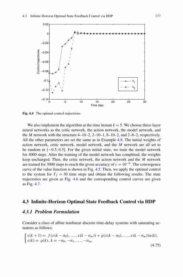
4.3 Infinite-Horizon Optimal State Feedback Control via HDP 177
Fig. 4.4 The optimal control trajectories
We also implement the algorithm at the time instant k = 5. We choose three-layerneural networks as the critic network, the action network, the model network, andthe M network with the structure 4–10–2, 2–10–1, 8–10–2, and 2–8–2, respectively.All the other parameters are set the same as in Example 4.8. The initial weights ofaction network, critic network, model network, and the M network are all set tobe random in [−0.5,0.5]. For the given initial state, we train the model networkfor 4000 steps. After the training of the model network has completed, the weightskeep unchanged. Then, the critic network, the action network and the M networkare trained for 3000 steps to reach the given accuracy of ε = 10−6. The convergencecurve of the value function is shown in Fig. 4.5. Then, we apply the optimal controlto the system for Tf = 30 time steps and obtain the following results. The statetrajectories are given as Fig. 4.6 and the corresponding control curves are givenas Fig. 4.7.
4.3 Infinite-Horizon Optimal State Feedback Control via HDP
4.3.1 Problem Formulation
Consider a class of affine nonlinear discrete time-delay systems with saturating ac-tuators as follows:{x(k + 1)= f (x(k − σ0), . . . , x(k − σm))+ g(x(k − σ0), . . . , x(k − σm))u(k),
x(k)= �(k), k = −σ0,−σ1, . . . ,−σm,
(4.75)
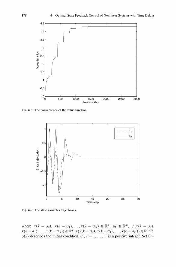
178 4 Optimal State Feedback Control of Nonlinear Systems with Time Delays
Fig. 4.5 The convergence of the value function
Fig. 4.6 The state variables trajectories
where x(k − σ0), x(k − σ1), . . . , x(k − σm) ∈ Rn, uk ∈ R
m, f (x(k − σ0),
x(k − σ1), . . . , x(k − σm)) ∈ Rn, g(x(k − σ0), x(k − σ1), . . . , x(k − σm)) ∈ R
n×m,�(k) describes the initial condition. σi , i = 1, . . . ,m is a positive integer. Set 0 =
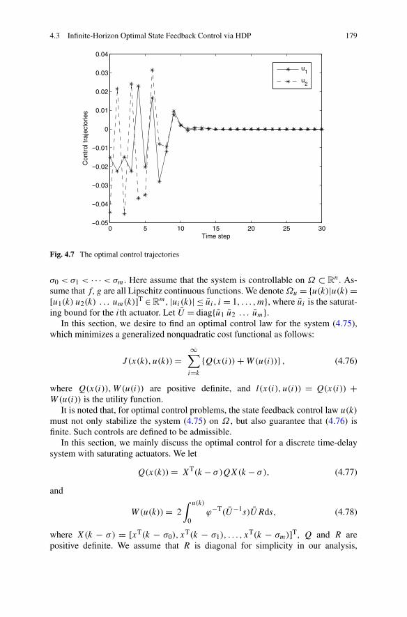
4.3 Infinite-Horizon Optimal State Feedback Control via HDP 179
Fig. 4.7 The optimal control trajectories
σ0 < σ1 < · · · < σm. Here assume that the system is controllable on Ω ⊂ Rn. As-
sume that f,g are all Lipschitz continuous functions. We denote Ωu = {u(k)|u(k)=[u1(k) u2(k) . . . um(k)]T ∈ R
m, |ui(k)| ≤ ui , i = 1, . . . ,m}, where ui is the saturat-ing bound for the ith actuator. Let U = diag{u1 u2 . . . um}.
In this section, we desire to find an optimal control law for the system (4.75),which minimizes a generalized nonquadratic cost functional as follows:
J (x(k), u(k))=∞∑
i=k
{Q(x(i))+W(u(i))} , (4.76)
where Q(x(i)),W(u(i)) are positive definite, and l(x(i), u(i)) = Q(x(i)) +W(u(i)) is the utility function.
It is noted that, for optimal control problems, the state feedback control law u(k)
must not only stabilize the system (4.75) on Ω , but also guarantee that (4.76) isfinite. Such controls are defined to be admissible.
In this section, we mainly discuss the optimal control for a discrete time-delaysystem with saturating actuators. We let
Q(x(k))= XT(k − σ)QX(k − σ), (4.77)
and
W(u(k))= 2∫ u(k)
0ϕ−T(U−1s)URds, (4.78)
where X(k − σ) = [xT(k − σ0), xT(k − σ1), . . . , x
T(k − σm)]T, Q and R arepositive definite. We assume that R is diagonal for simplicity in our analysis,
180 4 Optimal State Feedback Control of Nonlinear Systems with Time Delays
s ∈ Rm, ϕ ∈ R
m, ϕ−1(u(k)) = [ψ−1(u1(k)) ψ−1(u2(k)) · · · ψ−1(um(k))]T, ψ(·)
is a bounded single mapping function satisfying |ψ(·)| ≤ 1 and belonging to Cp
(p ≥ 1) and L2. Moreover, it is a monotonically increasing odd function with its firstderivative bounded by a constant M . We know that the hyperbolic tangent functionψ(·) = tanh(·) is one example of such functions. Noting that, W(u(k)) is ensuredto be positive definite by the definition above, because ψ−1(·) is a monotonic oddfunction, and R is positive definite.
Let J ∗(x(k))= minu(k) J (x(k), u(k)) denote the optimal value function, and letu∗(k) denote the corresponding optimal control law. According to Bellman’s prin-ciple of optimality, the optimal value function J ∗(x(k)) should satisfy the followingHJB equation:
J ∗(x(k))= minu(k)
∞∑
i=k
{Q(x(i)) + W(u(i))}
= minu(k)
{Q(x(k)) + W(u(k))+ J ∗(x(k + 1))}, (4.79)
and the optimal controller u∗(k) should satisfy
u∗(k)= arg minu(k)
∞∑
i=k
{Q(x(i)) + W(u(i))}
= arg minuk
{Q(x(k)) + W(u(k))+ J ∗(x(k + 1))}. (4.80)
The optimal control problem for the nonlinear discrete time-delay system withsaturating actuators can be solved if the optimal value function J ∗(x(k)) can be ob-tained from (4.79). However, there is currently no quite effective method for solvingthis value function for the nonlinear discrete time-delay system with saturating ac-tuators. Therefore, in the following we will discuss how to utilize the iterative HDPalgorithm to seek the approximate optimal control solution.
4.3.2 Optimal Control Based on Iterative HDP
First, for any given initial state �(k) and initial control law β(k), we start with theinitial iterative value function V [0](·) = 0. Then, we find the control vector u[0](k)as follows:
u[0](k)= arg minu(k)
{XT(k − σ)QX(k − σ)+ 2
∫ u(k)
0ϕ−T(U−1s)URds
+ V [0](x(k + 1))
}, (4.81)
4.3 Infinite-Horizon Optimal State Feedback Control via HDP 181
and the value function is updated as
V [1](x(k))= minu(k)
{XT(k − σ)QX(k − σ)+ 2
∫ u(k)
0ϕ−T(U−1s)URds
+ V [0](x(k + 1))
}, (4.82)
where x(1), . . . , x(k) are obtained under the action β(k), and
x(k + 1)= f (x(k − σ0), . . . , x(k − σm))
+ g(x(k − σ0), . . . , x(k − σm))u[0](k). (4.83)
Moreover, for i = 1,2, . . . , the iterative HDP algorithm iterates between
u[i](k)= arg minu(k)
{XT(k − σ)QX(k − σ)+ 2
∫ u(k)
0ϕ−T(U−1s)URds
+ V [i](x(k + 1))
}(4.84)
and
V [i+1](x(k))= minu(k)
{XT(k − σ)QX(k − σ)+ 2
∫ u(k)
0ϕ−T(U−1s)URds
+ V [i](x(k + 1))
}, (4.85)
where x(1), . . . , x(k) are obtained under the action u[i−1](k), and
x(k + 1)= f (x(k − σ0), . . . , x(k − σm))
+ g(x(k − σ0), . . . , x(k − σm))u[i](k). (4.86)
We further compute the control law u[i](k) from (4.84) as follows:
u[i](k)
= Uϕ
(−1
2(UR)−1gT(x(k − σ0), . . . , x(k − σm))
∂V [i](x(k+1))
∂x(k + 1)
), (4.87)
and update the value function as
V [i+1](x(k))= XT(k − σ)QX(k − σ)+ 2∫ u[i](k)
0ϕ−T(U−1s)URds
+ V [i](x(k + 1)). (4.88)
182 4 Optimal State Feedback Control of Nonlinear Systems with Time Delays
In the iterative HDP algorithm, the value function and control law are updated byrecurrent iteration, with the iteration number i increasing from 0 to ∞.
In the following, we give the convergence analysis of the present iterative HDPalgorithm for nonlinear discrete time-delay systems with saturating actuators theo-retically.
Lemma 4.10 Let {μ[i](k)} be an arbitrary sequence of control laws, and {u[i](k)}be the control law sequence expressed as in (4.84). Let V [i] be as in (4.85) and Λ[i]as
Λ[i+1](x(k))= XT(k − σ)QX(k − σ)+ 2∫ μ[i](k)
0ϕ−T(U−1s)URds
+Λ[i](x(k + 1)), (4.89)
where x(k + 1) is obtained under the action of μ[i](k). For the same initial state�(k) and initial control law β(k), if V [0](·) = Λ[0](·) = 0, then V [i+1](x(k)) ≤Λ[i+1](x(k)),∀i.
Proof It is straightforward from the fact that V [i+1] is a result of minimizing theright hand side of equation (4.85) with respect to the control input u[i](k), whileΛ[i+1] is the result of an arbitrary control input. �
Theorem 4.11 (cf. [3]) Let the sequence V [i+1](x(k)) be defined by (4.85). If thesystem is controllable, then there is an upper bound Y such that 0 ≤ V [i+1](x(k))≤Y , ∀i.
Proof Let {γ [i](k)} be any stabilizing and admissible control input, and let V [0](·)=P [0](·)= 0, where V [i+1](x(k)) is updated as (4.85) and P [i+1](x(k)) is updated as
P [i+1](x(k))= XT(k − σ)QX(k − σ)+ 2∫ γ [i](k)
0ϕ−T(U−1s)URds
+ P [i](x(k + 1)), (4.90)
where x(1), . . . , x(k) are obtained under the action γ [i−1](k), and x(k + 1) is ob-tained under the action of γ [i](k). From (4.90), we further obtain
P [i](x(k + 1))= XT(k − σ + 1)QX(k − σ + 1)
+ 2∫ γ [i−1](k+1)
0ϕ−T(U−1s)URds
+ P [i−1](x(k + 2)). (4.91)
4.3 Infinite-Horizon Optimal State Feedback Control via HDP 183
Thus, we obtain
P [i+1](x(k))= XT(k − σ)QX(k − σ)+ 2∫ γ [i](k)
0ϕ−T(U−1s)URds
+ XT(k − σ + 1)QX(k − σ + 1)
+ 2∫ γ [i−1](k+1)
0ϕ−T(U−1s)URds
+ · · ·+ XT(k − σ + i)QX(k − σ + i)
+ 2∫ γ [0](k+i)
0ϕ−T(U−1s)URds.
(4.92)
Let
L[i−j ](x(k + j))= XT(k − σ + j)QX(k − σ + j)
+ 2∫ γ [i−j ](k+j)
0ϕ−T(U−1s)URds, (4.93)
and then (4.92) can further be written as
P [i+1](x(k))=i∑
j=0
L[i−j ](x(k + j))
=i∑
j=0
{XT(k − σ + j)QX(k − σ + j)
+ 2∫ γ [i−j ](k+j)
0ϕ−T(U−1s)URds
}. (4.94)
Noticing that {γ [i](k)} is an admissible control law sequence, there exists an upperbound Y such that
P [i+1](x(k))≤ limi→∞
i∑
j=0
L[i−j ](x(k + j))≤ Y, ∀i. (4.95)
Thus, based on the definition of the cost functional and Lemma 4.10, we obtain
0 ≤ V [i+1](x(k))≤ P [i+1](x(k))≤ Y, ∀i. (4.96)
This completes the proof. �
184 4 Optimal State Feedback Control of Nonlinear Systems with Time Delays
Theorem 4.12 Define the value function sequence {V [i]} as in (4.85) withV [0](·) = 0, the control law sequence {u[i](k)} as in (4.84). Then, we concludethat {V [i]} is a nondecreasing sequence satisfying V [i+1](x(k))≥ V [i](x(k)), ∀i.
Proof We define a new sequence {Φ[i](x(k))} as follows:
Φ[i](x(k))= XT(k − σ)QX(k − σ)+ 2∫ u[i](k)
0ϕ−T(U−1s)URds
+Φ[i−1](x(k + 1)), (4.97)
where Φ[0](·)= V [0](·)= 0.In the following part, we prove Φ[i](x(k))≤ V i+1(x(k)) by mathematical induc-
tion.First,we prove that it holds for i = 0. Noticing that
V [1](x(k))−Φ[0](x(k))
= XT(k − σ)QX(k − σ)+ 2∫ u[0](k)
0ϕ−T(U−1s)URds
≥ 0, (4.98)
for i = 0, we get
V [1](x(k))≥Φ[0](x(k)). (4.99)
Second, we suppose that V [i](x(k))≥Φ[i−1](x(k)), for i−1, ∀x(k). Then, for i,since
V [i+1](x(k))= XT(k − σ)QX(k − σ)
+ 2∫ u[i](k)
0ϕ−T(U−1s)URds + V [i](x(k + 1)), (4.100)
and
Φ[i](x(k))= XT(k − σ)QX(k − σ)
+ 2∫ u[i](k)
0ϕ−T(U−1s)URds +Φ[i−1](x(k + 1)), (4.101)
we get
V [i+1](x(k))−Φ[i](x(k))= V [i](x(k + 1))−Φ[i−1](x(k + 1))≥ 0. (4.102)
Therefore, by mathematical induction, we have
V [i+1](x(k))≥Φ[i](x(k)),∀i. (4.103)
4.3 Infinite-Horizon Optimal State Feedback Control via HDP 185
In addition, from Lemma 4.10 we know that V [i](x(k))≤Φ[i](x(k)). Therefore,we have
V [i](x(k))≤Φ[i](x(k))≤ V [i+1](x(k)), (4.104)
which proves that {V [i](x(k))} is a nondecreasing sequence bounded by (4.96). �
Theorem 4.13 According to Theorem 4.11, there is a limit for the value func-tion sequence {V [i](x(k))} when i → ∞. Without loss of generality, we definelimi→∞ V [i](x(k)) = J ∗(x(k)), and, accordingly, limi→∞ u[i](k) = u∗(k). Then,for any discrete time step k, the limit J ∗(x(k)) is the “optimal” value function, i.e.,
J ∗(x(k))= minu(k)
{Q(x(k))+W(u(k))+ J ∗(x(k + 1))
}. (4.105)
Proof For any i, the value function sequence satisfies
V [i+1](x(k))= minu(k)
{Q(x(k))+W(u(k))+ V [i](x(k + 1))
}. (4.106)
Combining with V [i+1](x(k))≤limi→∞ V [i+1](x(k)),∀i, and limi→∞ V [i+1](x(k))= J ∗(x(k)), we obtain
J ∗(x(k))≥ minu(k)
{Q(x(k))+W(u(k))+ V [i](x(k + 1))
}
=Q(x(k))+W(u[i](k))+ V [i](x(k + 1)). (4.107)
Let i → ∞, we have
J ∗(x(k))≥Q(x(k))+W(u∗(k))+ J ∗(x(k + 1)). (4.108)
On the other hand, for any i and u[i](k), we have
V [i+1](x(k))≤Q(x(k))+W(u[i](k))+ V [i](x(k + 1)). (4.109)
As V [i](x(k))≤ V [i+1](x(k)), we obtain
V [i](x(k))≤Q(x(k))+W(u[i](k))+ V [i](x(k + 1)). (4.110)
Let i → ∞, we have
J ∗(x(k))≤Q(x(k))+W(u[i](k))+ J ∗(x(k + 1)). (4.111)
Since u[i](k) in the above equation is chosen arbitrarily, we have
J ∗(x(k))≤Q(x(k))+W(u∗(k))+ J ∗(x(k + 1)). (4.112)
186 4 Optimal State Feedback Control of Nonlinear Systems with Time Delays
Thus, we further obtain
J ∗(x(k))= Q(x(k))+W(u∗(k))+ J ∗(x(k + 1))
=minu(k)
{Q(x(k))+W(u(k))+ J ∗(x(k + 1))
}. (4.113)
This completes the proof. �
Therefore, we conclude that the value function sequence {V [i]} converges to theoptimal value function of the discrete-time HJB equation, i.e., V [i] → J ∗ as i → ∞.Simultaneously, we conclude that the corresponding control law sequence {u[i](k)}converges to the optimal control law u∗(k) as i → ∞.
4.3.3 Simulations
Example 4.14 Consider the following two-order nonlinear discrete time-delay sys-tem with saturating actuators:
{x(k + 1)= f (x(k), x(k − 2))+ g(x(k), x(k − 2))u(k), k ≥ 0x(k)= �(k), k = 0,−1,−2,
(4.114)
where f (x(k), x(k − 2)) = [ 0.2x1(k−2) exp(x22 (k))
0.3(x32 (k))
], g(x(k), x(k − 2)) = [ 0
−0.2
], and
assume that the control constraint is set to |u(k)| ≤ 0.3.Define the cost functional as
J (x(k))=∞∑
i=k
{XT(i − σ)QX(i − σ)+ 2
∫ u(i)
0tanh−T(U−1s)URds
},
(4.115)
where X(i − σ) = [xT(i), xT(i − 2)]T, x(i) = [x1(i), x2(i)]T, Q = I4, R = 0.5.The initial condition �(k) = [1.5 0.5]T, k = 0,−1,−2. Moreover, we implementthe algorithm at the time step k = 2.
In the presented iterative HDP algorithm, we choose three-layer neural networksas the critic network and the action network with the structure 2-8-1 and 4-8-1. Theinitial weight matrices are chosen randomly from [−0.1,0.1]. The critic networkand the action network are trained with the learning rates αa = αc = 0.01. After5000 iteration steps we get the curves of states, control input, and value function.The state trajectories are given as Fig. 4.8, and the corresponding control curve is
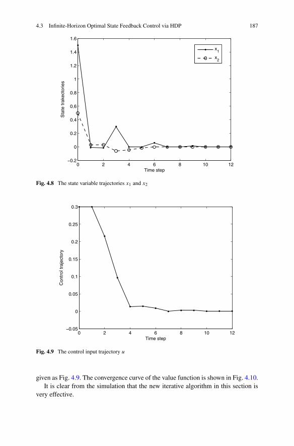
4.3 Infinite-Horizon Optimal State Feedback Control via HDP 187
Fig. 4.8 The state variable trajectories x1 and x2
Fig. 4.9 The control input trajectory u
given as Fig. 4.9. The convergence curve of the value function is shown in Fig. 4.10.It is clear from the simulation that the new iterative algorithm in this section is
very effective.
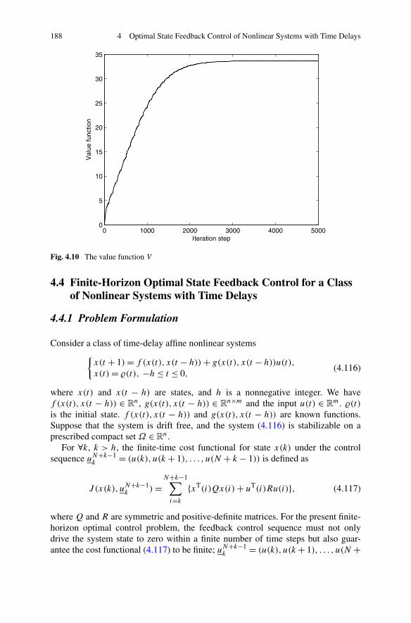
188 4 Optimal State Feedback Control of Nonlinear Systems with Time Delays
Fig. 4.10 The value function V
4.4 Finite-Horizon Optimal State Feedback Control for a Classof Nonlinear Systems with Time Delays
4.4.1 Problem Formulation
Consider a class of time-delay affine nonlinear systems{x(t + 1)= f (x(t), x(t − h))+ g(x(t), x(t − h))u(t),
x(t)= �(t), −h≤ t ≤ 0,(4.116)
where x(t) and x(t − h) are states, and h is a nonnegative integer. We havef (x(t), x(t − h)) ∈ R
n, g(x(t), x(t − h)) ∈ Rn×m and the input u(t) ∈ R
m. �(t)is the initial state. f (x(t), x(t − h)) and g(x(t), x(t − h)) are known functions.Suppose that the system is drift free, and the system (4.116) is stabilizable on aprescribed compact set Ω ∈R
n.For ∀k, k > h, the finite-time cost functional for state x(k) under the control
sequence uN+k−1k = (u(k), u(k + 1), . . . , u(N + k − 1)) is defined as
J (x(k), uN+k−1k )=
N+k−1∑
i=k
{xT(i)Qx(i)+ uT(i)Ru(i)}, (4.117)
where Q and R are symmetric and positive-definite matrices. For the present finite-horizon optimal control problem, the feedback control sequence must not onlydrive the system state to zero within a finite number of time steps but also guar-antee the cost functional (4.117) to be finite; uN+k−1
k = (u(k), u(k+ 1), . . . , u(N +
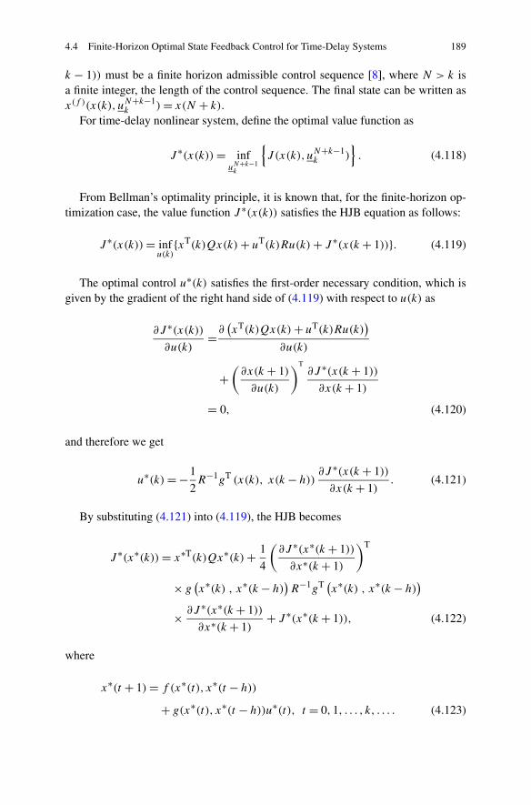
4.4 Finite-Horizon Optimal State Feedback Control for Time-Delay Systems 189
k − 1)) must be a finite horizon admissible control sequence [8], where N > k isa finite integer, the length of the control sequence. The final state can be written asx(f )(x(k), uN+k−1
k )= x(N + k).For time-delay nonlinear system, define the optimal value function as
J ∗(x(k))= infuN+k−1k
{J (x(k), uN+k−1
k )}. (4.118)
From Bellman’s optimality principle, it is known that, for the finite-horizon op-timization case, the value function J ∗(x(k)) satisfies the HJB equation as follows:
J ∗(x(k))= infu(k)
{xT(k)Qx(k)+ uT(k)Ru(k)+ J ∗(x(k + 1))}. (4.119)
The optimal control u∗(k) satisfies the first-order necessary condition, which isgiven by the gradient of the right hand side of (4.119) with respect to u(k) as
∂J ∗(x(k))∂u(k)
=∂(xT(k)Qx(k)+ uT(k)Ru(k)
)
∂u(k)
+(∂x(k + 1)
∂u(k)
)T∂J ∗(x(k + 1))
∂x(k + 1)
= 0, (4.120)
and therefore we get
u∗(k)= −1
2R−1gT (x(k), x(k − h))
∂J ∗(x(k + 1))
∂x(k + 1). (4.121)
By substituting (4.121) into (4.119), the HJB becomes
J ∗(x∗(k))= x∗T(k)Qx∗(k)+ 1
4
(∂J ∗(x∗(k + 1))
∂x∗(k + 1)
)T
× g(x∗(k) , x∗(k − h)
)R−1gT (x∗(k) , x∗(k − h)
)
× ∂J ∗(x∗(k + 1))
∂x∗(k + 1)+ J ∗(x∗(k + 1)), (4.122)
where
x∗(t + 1)= f (x∗(t), x∗(t − h))
+ g(x∗(t), x∗(t − h))u∗(t), t = 0,1, . . . , k, . . . . (4.123)
190 4 Optimal State Feedback Control of Nonlinear Systems with Time Delays
4.4.2 Optimal Control Based on Improved Iterative ADP
In this section, we apply the improved ADP algorithm to solve the finite-horizonvalue function and obtain an optimal control sequence (uN+k−1
k )∗ = (u∗(k),u∗(k + 1), . . . , u∗(N + k − 1)).
From system (4.116), we can see that for ∀k, and any initial state �(k), thereexists a control vector u(k), such that x(k + 1) = 0, i.e., we can control the stateof system (4.116) to zero in one step from any initial state. In the iterative ADPalgorithm, the value function and control law are updated by recursive iterations,with the iteration index number i increasing from 0 to ∞. The initial value functionV [0] = 0, and u[0](k) is an arbitrary control law.
The value function for i = 1 is computed as
V [1](x[0](k))= infu(k)
{x[0]T(k)Qx[0](k)+ uT(k)Ru(k)}
= x[0]T(k)Qx[0](k)+ u[1]T(k)Ru[1](k)
s.t. f (x[0](k), x[0](k − h))+ g(x[0](k), x[0](k − h))u(k)= 0, (4.124)
where
u[1](k)= arg infu(k)
{x[0]T(k)Qx[0](k)+ uT(k)Ru(k)}, (4.125)
and
x[0](t + 1)=
⎧⎪⎪⎪⎨
⎪⎪⎪⎩
f (x[1](t), x[1](t − h))
+g(x[1](t), x[1](t − h))u[2](t), k ≤ t
f (x[0](t), x[0](t − h))
+g(x[0](t), x[0](t − h))u[0](t), 0 ≤ t < k
x[0](t)=�(t), −h≤ t < 0. (4.126)
For i = 1,2, . . . , the value function V [i+1](x[i](k)) is updated as follows:
V [i+1](x[i](k))= infu(k)
{x[i]T(k)Qx[i](k)+ uT(k)Ru(k)
+ V [i](x[i−1](k + 1))}. (4.127)
The control law is updated as follows:
u[i+1](k)= arg infu(k)
{x[i]T(k)Qx[i](k)+ uT(k)Ru(k)
+ V [i](x[i−1](k + 1))}, (4.128)
4.4 Finite-Horizon Optimal State Feedback Control for Time-Delay Systems 191
where
x[i](t + 1)=
⎧⎪⎪⎨
⎪⎪⎩
f (x[i+1](t), x[i+1](t − h))
+g(x[i+1](t), x[i+1](t − h))u[i+2](t), k ≤ t,
f (x[i](t), x[i](t − h))
+g(x[i](t), x[i](t − h))u[i](t), 0 ≤ t < k,
x[i](t)= �(t), −h≤ t < 0. (4.129)
In this part, we present several theorems to demonstrate that the improved iter-ative ADP algorithm is convergent. Furthermore, the iterative value function con-verges to the optimal one.
Lemma 4.15 Let V [1](x[0](k)) be defined as (4.124), and V [i+1](x[i](k)) be definedas (4.127). Let uk+i
k be any finite-horizon admissible control sequence. Define
L[i+1](x[i](k), uk+ik )
= x[i]T(k)Qx[i](k)+ u[i+1]T(k)Ru[i+1](k)
+ x[i−1]T(k + 1)Qx[i−1](k + 1)+ u[i]T(k + 1)Ru[i](k + 1)+ · · ·+ x[0]T(k + i)Qx[0](k + i)+ u[1]T(k + i)Ru[1](k + i),
s.t. f (x[0](k + i), x[0](k + i − h))
+ g(x[0](k + i), x[0](k + i − h))u[1](k + i)= 0, (4.130)
and the final state under uk+ik satisfies
xf (x[i](k), uk+ik )= 0. (4.131)
If u[0](k)= u[0](k), then we have for ∀x[i](k)
V [i+1](x[i](k))= infuk+ik
{L[i+1] (x[i](k), uk+i
k
)}. (4.132)
Proof From (4.127) and (4.130), we easily get (4.132). �
Theorem 4.16 (cf. [2]) For system (4.116), let x(k), k > h, be an arbitrary statevector. Then, the value function sequence {V [i+1](x[i](k))} is a monotonically non-increasing sequence for i ≥ 1, i.e., V [i+1](x[i](k))≤ V [i](x[i−1](k)) for i ≥ 1.
Proof In (4.130), we let u[i+1](k) = u[i](k), and then we have x[i](k) = x[i−1](k).So we further obtain
L[i+1](x[i](k), uk+ik )
= x[i−1]T(k)Qx[i−1](k)+ u[i]T(k)Ru[i](k)
192 4 Optimal State Feedback Control of Nonlinear Systems with Time Delays
+ x[i−2]T(k + 1)Qx[i−2](k + 1)+ u[i−1]T(k + 1)Ru[i−1](k + 1)+ · · ·+ x[0]T(k + i − 1)Qx[0](k + i − 1)+ u[1]T(k + i − 1)Ru[1]T(k + i − 1),
+ x[0]T(k + i)Qx[0](k + i)+ u[1]T(k + i)Ru[1](k + i). (4.133)
From (4.124) and (4.125), we have known that x[0](k + i)= 0 and u[1](k + i)= 0.So we have
L[i+1](x[i](k), uk+ik )= V [i+1](x[i](k)). (4.134)
From Lemma 4.15, we have V i+1(x[i](k))≤ L[i+1](x[i](k), uk+ik ). So we obtain
V [i+1](x[i](k))≤ V [i](x[i−1](k)). (4.135)
This completes the proof. �
From Theorem 4.16, we can see that the value function V [i+1](x[i](k)) is a mono-tonically nonincreasing sequence and the lower bound is 0. In the following part,we will demonstrate that the limit of V [i+1](x[i](k)) satisfies HJB. The followinglemma is necessary for the further proof.
Lemma 4.17 Let V [i+1](x[i](k)) and u[i](k) be defined as (4.127) and (4.128). Let{μ[i](k)} be an arbitrary sequence of the control law, Λ[i+1](x[i](k)) be defined by
Λ[i+1](x[i](k))= x[i]T(k)Qx[i] +μ[i+1]T(k)Rμ[i+1](k)
+Λ[i](x[i−1](k + 1)), i > 0, (4.136)
with the first iteration expressed as follows:
Λ[1](x[0](k))= x[0]T(k)Qx[0](k)+μ[1]T(k)Rμ[1](k)
s.t. f (x[0](k), x[0](k − h))
+ g(x[0](k), x[0](k − h))μ[1](k)= 0, (4.137)
where
x[0](t + 1)=
⎧⎪⎪⎪⎨
⎪⎪⎪⎩
f (x[1](t), x[1](t − h))
+g(x[1](t), x[1](t − h))μ[2](t), t ≥ k
f (x[0](t), x[0](t − h))
+g(x[0](t), x[0](t − h))μ[0](t), 0 ≤ t < k
x[0](t)= �(t), −h≤ t ≤ 0, (4.138)
4.4 Finite-Horizon Optimal State Feedback Control for Time-Delay Systems 193
and for i ≥ 0, the state is updated as follows:
x[i](t + 1)=
⎧⎪⎪⎪⎨
⎪⎪⎪⎩
f (x[i+1](t), x[i+1](t − h))
+g(x[i+1](t), x[i+1](t − h))μ[i+2](t), t ≥ k
f (x[i](t), x[i](t − h))
+g(x[i](t), x[i](t − h))μ[i](t), 0 ≤ t < k
x[i](t)= �(t), −h≤ t ≤ 0. (4.139)
If u[0](k) = μ[0](k), and V [0] = Λ[0] = 0, then V [i+1](x[i−1](k)) ≤Λ[i+1](x[i−1](k)),∀i.
Proof It can be straightforwardly seen from the fact that V [i+1](x[i](k)) is the re-sult of minimizing the right hand side of (4.127) with respect to the control inputu[i+1](k), while Λ[i+1](x[i](k)) is the result of arbitrary control input. �
Theorem 4.18 For system (4.116), let x(k), k > h, be an arbitrary state vector.Let u∞(k) = limi→∞ u[i](k), and V∞(x∞(k)) = limi→∞ V [i+1](x[i](k)), wherex∞(k) is the state under the action of u∞(k). Then, we have
V∞(x∞(k))= infu(k)
{x∞T(k)Qx∞(k)+ uT(k)Qu(k)+ V∞(x∞(k + 1))}
= x∞T(k)Qx∞(k)+ u∞T(k)Qu∞(k)
+ V∞(x∞(k + 1)), (4.140)
where
u∞(k)= arg infu(k)
{x∞T(k)Qx∞(k)+ uT(k)Qu(k)+ V∞(x∞(k + 1))}. (4.141)
Proof Let {μ[i](k)} be arbitrary sequence of control law, and Λ[i+1](x[i](k)) bedefined as (4.136). Then, from Lemma 4.17, we get
V [i+1](x[i](k))≤ x[i]T(k)Qx[i](k)+μ[i+1]T(k)Rμ[i+1](k)
+Λ[i](x[i−1](k + 1)). (4.142)
Let {μ[i](k)} = {u[i](k)}; then (4.142) can be changed to
V [i+1](x[i](k))≤ x[i]T(k)Qx[i](k)+ u[i+1]T(k)Ru[i+1](k)+ V [i](x[i−1](k + 1))
= infu(k)
{x[i]T(k)Qx[i](k)+ uT(k)Ru(k)
+ V [i](x[i−1](k + 1))}. (4.143)
194 4 Optimal State Feedback Control of Nonlinear Systems with Time Delays
Let i → ∞ in (4.143), we obtain
V∞(x∞(k))≤ infu(k)
{x∞T(k)Qx∞(k)+ uT(k)Qu(k)
+ V∞(x∞(k + 1))}. (4.144)
According to Theorem 4.16, we have V [i+1](x[i](k))≤ V [i](x[i−1](k)), i.e.,
V [i](x[i−1](k))≥ infu(k)
{x[i]T(k)Qx[i](k)+ uT(k)Ru(k)
+ V [i](x[i−1](k + 1))}. (4.145)
Let i → ∞ in (4.145), and we obtain
V∞(x∞(k))≥ infu(k)
{x∞T(k)Qx∞(k)+ uT(k)Qu(k)
+ V∞(x∞(k + 1))}. (4.146)
Thus, combining (4.144) and (4.146), we have
V∞(x∞(k))= infu(k)
{x∞T(k)Qx∞(k)+ uT(k)Qu(k)
+ V∞(x∞(k + 1))}. (4.147)
This completes the proof. �
Theorem 4.19 Let V∞(x∞(k)) = limi→∞ V [i+1](x[i](k)), and let V [i+1](x[i](k))be defined as (4.127). Then we have V∞(x∞(k))= J ∗(x∗(k)).
Proof From the definition of J ∗(x∗(k)), we get
J ∗(x∗(k))≤ V [i+1](x[i](k)). (4.148)
Let i → ∞ in (4.148); we have
J ∗(x∗(k))≤ V∞(x∞(k)). (4.149)
On the other hand, according to the definition J ∗(x∗(k)) in (4.119), for anyθ > 0, there exists a sequence of control law μ[i+1](k), such that the associ-ated value function Λ[i+1](x[i](k)) defined as (4.136) satisfies Λ[i+1](x[i](k)) ≤J ∗(x∗(k))+ θ . From Lemma 4.17, we get
V [i+1](x[i](k))≤Λ[i+1](x[i](k))≤ J ∗(x∗(k))+ θ. (4.150)
Let i → ∞; we obtain
V∞(x∞(k))≤ J ∗(x∗(k))+ θ. (4.151)
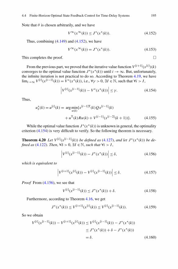
4.4 Finite-Horizon Optimal State Feedback Control for Time-Delay Systems 195
Note that θ is chosen arbitrarily, and we have
V∞(x∞(k))≤ J ∗(x∗(k)). (4.152)
Thus, combining (4.149) and (4.152), we have
V∞(x∞(k))= J ∗(x∗(k)). (4.153)
This completes the proof. �
From the previous part, we proved that the iterative value function V [i+1](x[i])(k)converges to the optimal value function J ∗(x∗(k)) until i → ∞. But, unfortunately,the infinite iteration is not practical to do so. According to Theorem 4.19, we havelimi→∞ V [i](x[i−1](k))= V ∗(x∗(k)), i.e., ∀γ > 0, ∃I ∈ N, such that ∀i > I ,
∣∣∣V [i](x[i−1](k))− V ∗(x∗(k))∣∣∣≤ γ. (4.154)
Thus,
u∗δ (k)= u[i](k)= arg min
u(k){x[i−1]T(k)Qx[i−1](k)
+ uT(k)Ru(k)+ V [i−1](x[i−2](k + 1))}. (4.155)
While the optimal value function J ∗(x∗(k)) is unknown in general, the optimalitycriterion (4.154) is very difficult to verify. So the following theorem is necessary.
Theorem 4.20 Let V [i](x[i−1](k)) be defined as (4.127), and let J ∗(x∗(k)) be de-fined as (4.122). Then, ∀δ > 0, ∃I ∈N, such that ∀i > I ,
∣∣∣V [i](x[i−1](k))− J ∗(x∗(k))∣∣∣≤ δ, (4.156)
which is equivalent to∣∣∣V [i+1](x[i](k))− V [i](x[i−1](k))
∣∣∣≤ δ. (4.157)
Proof From (4.156), we see that
V [i](x[i−1](k))≤ J ∗(x∗(k))+ δ. (4.158)
Furthermore, according to Theorem 4.16, we get
J ∗(x∗(k))≤ V [i+1](x[i](k))≤ V [i](x[i−1](k)). (4.159)
So we obtain
V [i](x[i−1](k))− V [i+1](x[i](k))≤ V [i](x[i−1](k))− J ∗(x∗(k))
≤ J ∗(x∗(k))+ δ − J ∗(x∗(k))
= δ. (4.160)
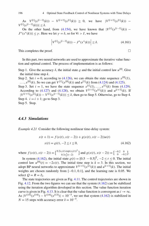
196 4 Optimal State Feedback Control of Nonlinear Systems with Time Delays
As V [i](x[i−1](k)) − V [i+1](x[i](k)) ≥ 0, we have |V [i+1](x[i](k)) −V [i](x[i−1](k))| ≤ δ.
On the other hand, from (4.154), we have known that |V [i](x[i−1](k)) −J ∗(x∗(k))| ≤ γ . Here we let γ = δ, so for ∀i > I , we have
∣∣∣V [i](x[i−1](k))− J ∗(x∗(k))∣∣∣≤ δ. (4.161)
This completes the proof. �
In this part, two neural networks are used to approximate the iterative value func-tion and optimal control. The process of implementation is as follows:
Step 1. Give the accuracy δ, the initial state � and the initial control law u[0]. Givethe initial time step k.
Step 2. Set i = 0, according to (4.126), we can obtain the state sequence x[0](1),. . . , x[0](k). So we can get V [1](x[0](k)) and u[1](k) from (4.124) and (4.125).
Step 3. Set i = 1, we have the state sequence x[i](1), . . . , x[i](k) from (4.129).According to (4.127) and (4.128), we obtain V [i+1](x[i](k)) and u[i+1](k). If|V [i+1](x[i](k))− V [i](x[i−1](k))| ≤ δ, then go to Step 5. Otherwise, go to Step 4.
Step 4. i = i + 1; go to Step 3.Step 5. Stop.
4.4.3 Simulations
Example 4.21 Consider the following nonlinear time-delay system:
x(t + 1)= f (x(t), x(t − 2))+ g(x(t), x(t − 2))u(t)
x(t)= �(t),−2 ≤ t ≤ 0, (4.162)
where f (x(t), x(t − 2))= [ 0.2x1(t) exp(x2(t))2
0.3x32 (t−2)
]and g(x(t), x(t − 2))= [−0.2 0
0 −0.2
].
In system (4.162), the initial state �(t) = [0.5 − 0.5]T, −2 ≤ t ≤ 0. The initialcontrol law u[0](t) = −2x(t). The initial time step is k = 3. In this section, weadopt BP neural networks to approximate V [i+1](x[i](k)) and u[i+1](k). The initialweights are chosen randomly from [−0.1,0.1], and the learning rate is 0.05. Weselect Q=R = I2.
The state trajectories are given as Fig. 4.11. The control trajectories are shown inFig. 4.12. From the two figures we can see that the system (4.162) can be stabilizedusing the iteration algorithm developed in this section. The value function iterationcurve is given in Fig. 4.13. It is clear that the value function is convergent as i → ∞.As |V [15](x[14])− V [14](x[13])| < 10−5, we see that system (4.162) is stabilized inN = 15 steps with accuracy error δ = 10−5.
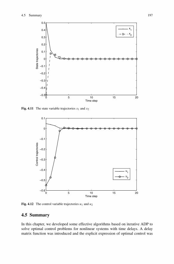
4.5 Summary 197
Fig. 4.11 The state variable trajectories x1 and x2
Fig. 4.12 The control variable trajectories u1 and u2
4.5 Summary
In this chapter, we developed some effective algorithms based on iterative ADP tosolve optimal control problems for nonlinear systems with time delays. A delaymatrix function was introduced and the explicit expression of optimal control was
198 4 Optimal State Feedback Control of Nonlinear Systems with Time Delays
Fig. 4.13 The value function
obtained. We then developed an effective algorithm to solve the optimal controlproblems for nonlinear time-delay systems with saturating actuators. Finally, an ef-fective algorithm to solve the finite-horizon optimal control problems was developedfor a class of time-delay systems. Simulation studies successfully demonstrated theoutstanding performance of the present optimal control schemes for time-delay non-linear systems.
References
1. Malek-Zavarei M, Jashmidi M (1987) Time-delay systems: analysis, optimization and appli-cations. North-Holland, Amsterdam, pp 80–96
2. Song RZ, Zhang HG (2011) The finite horizon optimal control for a class of time-delay affinenonlinear system. Neural Comput Appl. doi:10.1007/s00521-011-0706-3
3. Song RZ, Zhang HG, Wei QL, Luo YH (2010) Optimal control laws for time-delay sys-tems with saturating actuators based on heuristic dynamic programming. Neurocomputing73:3020–3027
4. Tong SC, Liu CL, Li YM, Zhang HG (2011) Adaptive fuzzy decentralized control for large-scale nonlinear systems with time-varying delays and unknown high-frequency gain sign.IEEE Trans Syst Man Cybern, Part B, Cybern 41:474–485
5. Wang ZS, Zhang HG (2010) Global asymptotic stability of reaction–diffusion Cohen–Grossberg neural networks with continuously distributed delays. IEEE Trans Neural Netw21:39–49
6. Wang ZS, Zhang HG, Li P (2010) An LMI approach to stability analysis of reaction–diffusionCohen–Grossberg neural networks concerning Dirichlet boundary conditions and distributeddelays. IEEE Trans Syst Man Cybern, Part B, Cybern 40:1596–1606
References 199
7. Wang YC, Zhang HG, Wang XY, Yang DS (2010) Networked synchronization control ofcoupled dynamic networks with time-varying delay. IEEE Trans Syst Man Cybern, Part B,Cybern 40:1468–1479
8. Wang FY, Jin N, Liu DR, Wei Q (2011) Adaptive dynamic programming for finite-horizonoptimal control of discrete-time nonlinear systems with ε-error bound. IEEE Trans NeuralNetw 22:24–36
9. Wei QL, Zhang HG, Liu DR, Zhao Y (2010) An optimal control scheme for a class of discrete-time nonlinear systems with time delays using adaptive dynamic programming. Acta AutomSin 36:121–129
10. Zhang HG, Wang YC (2008) Stability analysis of Markovian jumping stochastic Cohen–Grossberg neural networks with mixed time delays. IEEE Trans Neural Netw 19:366–370
11. Zhang HG, Xie YH, Wang ZL, Zheng CD (2007) Adaptive synchronization between twodifferent chaotic neural networks with time delay. IEEE Trans Neural Netw 18:1841–1845
12. Zhang HG, Wang ZS, Liu DR (2008) Robust stability analysis for interval Cohen–Grossbergneural networks with unknown time-varying delays. IEEE Trans Neural Netw 19:1942–1955
13. Zhang HG, Wang YC, Liu DR (2008) Delay-dependent guaranteed cost control for uncertainstochastic fuzzy systems with multiple tire delays. IEEE Trans Syst Man Cybern, Part B,Cybern 38:126–140
14. Zhang HG, Wei QL, Luo YH (2008) A novel infinite-time optimal tracking control schemefor a class of discrete-time nonlinear systems via the greedy HDP iteration algorithm. IEEETrans Syst Man Cybern, Part B, Cybern 38:937–942
15. Zheng CD, Zhang HG, Wang ZS (2009) New delay-dependent global exponential stabilitycriterion for cellular-type neural networks with time-varying delays. IEEE Trans Circuits SystII, Express Briefs 56:250–254
16. Zheng CD, Zhang HG, Wang ZS (2010) Improved robust stability criteria for delayed cellularneural networks via the LMI approach. IEEE Trans Circuits Syst II, Express Briefs 57:41–45
Chapter 5Optimal Tracking Control of Nonlinear Systemswith Time Delays
5.1 Introduction
Chapter 4 discussed the optimal state feedback control problems of nonlinear sys-tems with time delay. In this chapter, we will solve the optimal tracking controlproblem of nonlinear systems with time delay based on the HDP algorithm. First,the HJB equation for a discrete time-delay system is derived which is based on stateerror and control error. In order to solve this HJB equation, a novel iterative HDPalgorithm containing the iterations of state, control law, and cost functional is de-veloped. We also give the convergence proof for the novel iterative HDP algorithm.Finally, the critic network and action network are used to approximate the valuefunction and the corresponding control law, respectively. The main contributions ofthis chapter can be summarized as follows:
1. It is the first time that one solves the optimal tracking control problem of nonlin-ear systems with time delays using the HDP algorithm.
2. For the novel HDP algorithm, besides the value function iteration, the state isalso updated according to the iterative control law in every iteration step.
3. In the state update, we adopt “backward iteration”. For the (i + 1)st cost func-tional iteration, the state at time step k + 1 is updated according to the statesbefore time step k + 1 in the ith iteration and the control law in the ith iteration.
5.2 Problem Formulation
Consider a class of discrete-time affine nonlinear systems with time delays:
x(k + 1)= f (x(k − σ0), x(k − σ1), . . . , x(k − σm))
+ g(x(k − σ0), x(k − σ1), . . . , x(k − σm))u(k),
x(k)= �1(k), −σm ≤ k ≤ 0, (5.1)
H. Zhang et al., Adaptive Dynamic Programming for Control,Communications and Control Engineering, DOI 10.1007/978-1-4471-4757-2_5,© Springer-Verlag London 2013
201
202 5 Optimal Tracking Control of Nonlinear Systems with Time Delays
where x(k − σ0), x(k − σ1), . . . , x(k− σm) ∈Rn and x(k − σ1), . . . , x(k − σm) are
states of time delays. f (x(k − σ0), x(k − σ1), . . . , x(k − σm)) ∈ Rn,
g(x(k − σ0), x(k − σ1), . . . , x(k − σm)) ∈ Rn×m and the input u(k) ∈ R
m. �1(k)
is the initial state, σi is the time delay. We set 0 = σ0 < σ1 < · · · < σm, andthese are nonnegative integer numbers. f (x(k − σ0), x(k − σ1), . . . , x(k − σm))
and g(x(k− σ0), x(k− σ1), . . . , x(k− σm)) are known functions, and g(x(k− σ0),
x(k−σ1), . . . , x(k−σm)) is analytic. The system (5.1) is controllable and reachablein Ω ∈R
n [8].In this chapter, we define the state error as follows:
e(k)= x(k)− xd(k), (5.2)
where the reference orbit xd(k) is generated by the n-dimensional autonomous sys-tem as follows:
xd(k + 1)= S(xd(k)),
xd(0)= �2(k),−σm ≤ k ≤ 0, (5.3)
where xd(k) ∈ Rn, S(xd(k)) ∈ R
n and �2 is the initial state, �2(−σm) = · · · =�2(−σ1)= 0.
The objective in this chapter is to design an optimal state feedback control lawu(k) based on any given �1(k)(−σm ≤ k ≤ 0) and initial control law β(k), whichnot only renders the state x(k) asymptotically tracking the reference orbit, i.e., e(k)asymptotically approaches zero; it also minimizes the cost functional as follows:
J (e(k), v(k))=∞∑
i=k
{eT(i)Qe(i)+ vT(i)Rv(i)
}, (5.4)
where Q and R are symmetric and positive-definite matrices. We divide u(k) intotwo parts, i.e., v(k) and us(k). So we have
v(k)= u(k)− us(k), (5.5)
where us(k) denotes the steady control input corresponding to the desired trajectoryxd(k). In fact, v(k) is the error between actual control u(k) of system (5.1) and thesteady control us(k).
We see that the problem of solving the optimal tracking control law u(k) ofsystem (5.1) is converted into solving the optimal control law v(k). In the followingsection, we will discuss how to design v(k).
5.3 Optimal Tracking Control Based on Improved Iterative ADPAlgorithm
In this section, we focus on designing the optimal control law to handle the optimaltracking control problem. We first give a representation of the steady control input
5.3 Optimal Tracking Control Based on Improved Iterative ADP Algorithm 203
us(k). Inspired by the paper of [13], we define the steady control as follows:
us(k)= g−1(xd(k − σ0), . . . , xd(k − σm))
× (xd(k + 1)− f (xd(k − σ0), . . . , xd(k − σm))), (5.6)
where g−1(·) denotes the inversion of g(·).
Remark 5.1 If g(·) is invertible, then us can be obtained directly by (5.6). So usexists, when g(·) is invertible. If g(·) is noninvertible, us also exists. Because of thenumerical solution of g−1(·) can be solved at least by one of the three methods asfollows:
1. Moore–Penrose pseudoinverse technique [4]:The Moore–Penrose pseudoinverse is a matrix G of the same dimensions as g,
satisfying four conditions: gGg = g, GgG = G, Gg is Hermitian, and gG isHermitian.
In [4], it is proved that the matrix G exists and is unique, if g �= 0. In thischapter, g �= 0 obviously, because we supposed that the system (5.1) is control-lable and reachable. So we can say that g−1 = G. Furthermore, in Matlab 7.5,the Moore–Penrose pseudoinverse of g can be obtained by the Matlab functionG= pinv(g).
2. Least square method [2]:As g(·)g−1(·)= I , we have
g−1(·)= (gT(·)g(·))−1gT(·). (5.7)
Introducing E(0, r2) ∈Rn×m into g(·), g(·) can be expressed as follows:
g(·)= g(·)+E(0, r2), (5.8)
where every element in E(0, r2) is zero-mean Gaussian noise. So we get
g−1(·)= (gT(·)g(·))−1gT(·). (5.9)
Then, we sample K times, every time we take nm Gaussian points, so we haveEi(0, r2), i ∈ {1,2, . . . ,K}. Every element in Ei is a Gaussian sample point.Thus, we have G(·)= [g1; . . . ; gK ], where gi = g+Ei(0, r2), i ∈ {1,2, . . . ,K}.
So we get
g−1(·)= (GT(·)G(·))−1gT(·). (5.10)
3. Neural network method [11]:First, we let the BP neural network be expressed as F (X,V,W) =
WTσ(V TX), where W and V are the weights of the neural network and σ isthe activation function. Second, we use the output x(k + 1) of BP neural net-work to approximate x(k + 1). Then, we have x(k + 1) = WTσ(V TX), where
204 5 Optimal Tracking Control of Nonlinear Systems with Time Delays
X = [x(k), u(k)]. We already know that the system (5.1) is an affine nonlinearsystem. So we get g = ∂x(k + 1)/∂u. The equation g−1 = ∂u/∂x(k + 1) canalso be established.
So we can see that us is existent and can be obtained by (5.6). In this chapter, weadopt the Moore–Penrose pseudoinverse technique to get g−1(·) in our simulationsection.
According to (5.1), and in light of (5.2) with respect to x(k) and (5.5) with respectto us(k), we easily obtain
e(k + 1)= f (e(k − σ0)+ xd(k − σ0), . . . , e(k − σm)
+ xd(k − σm))+ g(e(k − σ0)+ xd(k − σ0),
. . . , e(k − σm)+ xd(k − σm))
× (g−1(xd(k − σ0), . . . , xd(k − σm))
× (S(xd(k))− f (xd(k − σ0), . . . , xd(k − σm)))
+ v(k))− S(xd(k)),
e(k)= �(k),−σm ≤ k ≤ 0, (5.11)
where �(k)= �1(k)− �2(k).So the aim for this chapter is changed to getting an optimal control law not only
making the system (5.11) asymptotically stable but also making the cost functional(5.4) minimal. To solve the optimal tracking control problem in this chapter, thefollowing definition and assumption are required.
Definition 5.2 (cf. [10]) (Asymptotic Stability) An equilibrium state e = 0 for sys-tem (5.11) is asymptotically stable if:
1. It is stable, i.e., given any positive numbers k0 and ε, there exists δ > 0, suchthat every solution of system (5.11) satisfies maxk0≤k≤k0+σm |e(k)| ≤ δ andmaxk0≤k≤∞ |e(k)| ≤ ε.
2. For each k0 > 0 there is a δ > 0 such that every solution of system (5.11) satisfiesmaxk0≤k≤k0+σm |e(k)| ≤ δ and limk→∞ e(k)= 0.
Assumption 5.3 Given the system (5.11), for the infinite-time horizon problem,there exists a control law v(k), which satisfies:
1. v(k) is continuous on Ω ; if e(k − σ0) = e(k − σ1) = · · · = e(k − σm) = 0, thenv(k)= 0;
2. v(k) stabilizes system (5.11);3. ∀e(−σ0), e(−σ1), e(−σm) ∈ R
n, J (e(0), v(0)) is finite.
Actually, for nonlinear systems without time delays, if v(k) satisfies Assump-tion 5.3, then we can say that v(k) is an admissible control. The definition of anadmissible control can be found in [3].
5.3 Optimal Tracking Control Based on Improved Iterative ADP Algorithm 205
In system (5.11), for time step k, J ∗(e(k)) is used to denote the optimal valuefunction, i.e., J ∗(e(k))= infv(k) J (e(k), v(k)), and the corresponding control inputcan be formulated as v∗(k) = arg infv(k) J (e(k), v(k)). Thus, we see that u∗(k) =v∗(k) + us(k) is the optimal control for system (5.1). Let e∗(k) = x∗(k) − xd(k),where x∗(k) is used to denote the state under the action of the optimal trackingcontrol law u∗(k).
According to Bellman’s principle of optimality [10], J ∗(e(k)) should satisfy thefollowing HJB equation:
J ∗(e(k))= infv(k)
{eT(k)Qe(k)+ vT(k)Rv(k)+ J ∗(e(k + 1))
}, (5.12)
i.e., the optimal controller v∗(k) should satisfy
v∗(k)= arg infv(k)
{eT(k)Qe(k)+ vT(k)Rv(k)+ J ∗(e(k + 1))
}. (5.13)
Here we define e∗(k)= x∗(k)− xd(k), and
x∗(k + 1)= f (x∗(k − σ0), . . . , x∗(k − σm))
+ g(x∗(k − σ0), . . . , x∗(k − σm))u
∗(k), k = 0,1,2, . . . ,
x∗(k)= �1(k), k = −σm,−σm−1, . . . ,−σ0. (5.14)
Then the HJB equation is written as follows:
J ∗(e∗(k))= e∗T(k)Qe∗(k)+ v∗T(k)Rv∗(k)+ J ∗(e∗(k + 1)). (5.15)
Remark 5.4 Of course, one can reduce system (5.1) to a system without time de-lay by defining a new (σm + 1)n-dimensional state vector y(k) = (x(k − σ0),
x(k − σ1), . . . , x(k − σm)). However, Chyung has pointed out that there are twomajor disadvantages of this method in [6]. First, the resulting new system is a(σm + 1)n-dimensional system increasing the dimension of the system by (σm + 1)fold. Second, the new system may not be controllable, even if the original system iscontrollable. This causes the set of attainability to have an empty interior which, inturn, introduces additional difficulties [5–7].
Therefore, in the following part, a direct method for time-delay systems is de-veloped for the optimal tracking control law. In the novel algorithm, we emphasizethat the states are regulated by the designed controller in each iteration. The detailediteration process is as follows.
First, we start with the initial value function V [0](·)= 0 which is not necessarilythe optimal value function. Then, for any given state �1(t) (−σm ≤ t ≤ 0), and initialcontrol β(t) in system (5.1), at any current time k, we start the iterative algorithmfrom i = 0 to find the control law v[0](k) as follows:
v[0](k)= arg infv(k)
{eT(k)Qe(k)+ vT(k)Rv(k)
}, (5.16)
206 5 Optimal Tracking Control of Nonlinear Systems with Time Delays
and the value function is updated as follows:
V [1](e(k))= infv(k)
{eT(k)Qe(k)+ vT(k)Rv(k)
}, (5.17)
where e(k)= x(k)− xd(k), and
x(t + 1)= f (x(t − σ0), . . . , x(t − σm))
+ g(x(t − σ0), . . . , x(t − σm))β(t)
x(t)= �1(t). − σm ≤ t ≤ 0. (5.18)
We notice that the states are generated by the designed controller, so we further getthe value function iteration as follows:
V [1](e[0](k))= e[0]T(k)Qe[0](k)+ v[0]T(k)Rv[0](k). (5.19)
For i = 1,2, . . . , the iterative HDP algorithm performs the iterations between
v[i](k)= arg infv(k)
{eT(k)Qe(k)+ vT(k)Rv(k)
+ V [i](e(k + 1))} (5.20)
and
V [i+1](e(k))= infv(k)
{eT(k)Qe(k)+ vT(k)Rv(k)
+ V [i](e(k + 1))}. (5.21)
It should be emphasized that the states in each iteration are regulated by thedesigned control law, so we further obtain
V [i+1](e[i](k))= e[i]T(k)Qe[i](k)+ v[i]T(k)Rv[i](k)
+ V [i](e[i−1](k + 1)), (5.22)
where e[i](k) = x[i](k) − xd(k), i = 0,1,2, . . . , and the states are updated as fol-lows:
x[i](t + 1)=
⎧⎪⎪⎪⎪⎪⎪⎪⎪⎨
⎪⎪⎪⎪⎪⎪⎪⎪⎩
f (x[i+1](t − σ0), . . . , x[i+1](t − σm))
+g(x[i+1](t − σ0), . . . , x[i+1](t − σm))
×u[i+1](t), t ≥ k,
f (x[i](t − σ0), . . . , x[i](t − σm))
+g(x[i](t − σ0), . . . , x[i](t − σm))
×u[i](t), 0 ≤ t < k,
x[i](t)= �1(t), −σm ≤ t ≤ 0, (5.23)
where u[i](t)= v[i](t)+ us(t).
5.3 Optimal Tracking Control Based on Improved Iterative ADP Algorithm 207
Remark 5.5 From (5.23) we find that the state x[i](t + 1), t ≥ k, is related tox[i+1](t − σ0), . . . , x
[i+1](t − σm) and u[i+1](t). It reflects the “backward iteration”of state at t, t ≥ k.
Remark 5.6 One important property we must point out is that the HDP algorithmdeveloped in this chapter is different from the algorithm presented in [13]:
1. The HDP algorithm presented in [13] deals with nonlinear systems without timedelays, while the HDP algorithm developed in this chapter deals with time-delaynonlinear systems.
2. For the HDP algorithm presented in [13], only the value function is updatedaccording to the control law iteration in every iteration step. For the HDP algo-rithm developed in this chapter, besides the value function iteration, the state isalso updated according to the control law iteration.
Based on the analysis above, our algorithm is a novel HDP algorithm. It is adevelopment of the HDP algorithm presented in [13].
In the following part, we present the convergence analysis of the iteration of(5.16)–(5.23).
Lemma 5.7 Let v[i](k) and V [i+1](e[i](k)) be expressed as (5.20) and (5.22), andlet {μ[i](k)} be arbitrary sequence of control law, and let Λ[i+1] be defined by
Λ[i+1](e[i](k))= e[i]T(k)Qe[i](k)+μ[i]T(k)Rμ[i](k)
+Λ[i](e[i−1](k + 1)), i ≥ 0. (5.24)
Thus, if V [0] =Λ[0] = 0, then V [i+1](e[i](k))≤Λ[i+1](e[i](k)),∀e[i](k).
Proof For given �1(t) (−σm ≤ t ≤ 0) of system (5.1), it can be straightforwardlyseen from the fact that V [i+1](e[i](k)) is obtained by the control input v[i](k), whileΛ[i+1](e[i](k)) is the result of arbitrary control input. �
Lemma 5.8 Let the sequence V [i+1](e[i](k)) be defined by (5.22); v[i](k) is thecontrol law expressed as (5.20). There is an upper bound Y , such that 0 ≤V [i+1](e[i](k))≤ Y , ∀e[i](k).
Proof Let γ [i](k) be any control law that satisfies Assumption 5.3. Let V [0] =P [0] = 0, and let P [i+1](e[i](k)) be defined as follows:
P [i+1](e[i](k))= e[i]T(k)Qe[i](k)+ (γ [i](k))TRγ [i](k)
+ P [i](e[i−1](k + 1)). (5.25)
From (5.25), we obtain
P [i](e[i−1](k + 1))= e[i−1]T(k + 1)Qe[i−1](k + 1)
208 5 Optimal Tracking Control of Nonlinear Systems with Time Delays
+ γ [i−1]T(k + 1)Rγ [i−1](k + 1)
+ P [i−1](e[i−2](k + 2)). (5.26)
Thus, we get
P [i+1](e[i](k))= e[i]T(k)Qe[i](k)
+ γ [i]T(k)Rγ [i](k)
+ e[i−1]T(k + 1)Qe[i−1](k + 1)
+ γ [i−1]T(k + 1)Rγ [i−1](k + 1)
+ · · ·+ e[0]T(k + i)Qe[0](k + i)
+ γ [0]T(k + i)Rγ [0](k + i). (5.27)
For j = 0, . . . , i, we let
L(k + j)= e[i−j ]T(k + j)Qe[i−j ](k + j)
+ γ [i−j ]T(k + j)Rγ [i−j ](k + j). (5.28)
Then (5.27) can further be written as follows:
P [i+1](e[i](k))=i∑
j=0
L(k + j). (5.29)
Furthermore, we see that
∀i : P [i+1](e[i](k))≤ limi→∞
i∑
j=0
L(k + j). (5.30)
Noting that {γ [i](k)} satisfies Assumption 5.3, according to the third condition ofAssumption 5.3, there exists an upper bound Y such that
limi→∞
i∑
j=0
L(k + j)≤ Y. (5.31)
From Lemma 5.7 we obtain
∀i : V [i+1](e[i](k))≤ P [i+1](e[i](k))≤ Y. (5.32)
This completes the proof. �
5.3 Optimal Tracking Control Based on Improved Iterative ADP Algorithm 209
Theorem 5.9 (cf. [12]) For system (5.1), the iterative algorithm is as in (5.16)–(5.23); then we have V [i+1](e[i](k))≥ V [i](e[i](k)), ∀e[i](k).
Proof For convenience in our analysis, define a new sequence {Φ[i](e(k))} as fol-lows:
Φ[i](e(k))= eT(k)Qe(k)+ v[i]T(k)Rv[i](k)
+Φ[i−1](e(k + 1)), (5.33)
with v[i](k) defined by (5.20), Φ[0](e(k))= 0.In the following part, we will prove Φ[i](e(k)) ≤ V [i+1](e(k)) by mathematical
induction.First, we prove that it holds for i = 0. Notice that
V [1](e(k))−Φ[0](e(k))= eT(k)Qe(k)v[0]T(k)Rv[0](k)
≥ 0, (5.34)
thus, for i = 0, we have
V [1](e(k))≥Φ[0](e(k)). (5.35)
Second, we assume that it holds for i, i.e., V [i](e(k))≥Φ[i−1](e(k)), for ∀e(k).Then, from (5.21) and (5.33), we get
V [i+1](e(k))−Φ[i](e(k))= V [i](e(k + 1))−Φ[i−1](e(k + 1))
≥ 0, (5.36)
i.e., the following inequality holds:
Φ[i](e(k))≤ V [i+1](e(k)). (5.37)
Therefore, (5.37) is proved by mathematical induction, for ∀e(k).On the other hand, from Lemma 5.7, we have ∀e[i](k), V [i+1](e[i](k)) ≤
Φ[i+1](e[i](k)). So we have V [i](e(k))≤Φ[i](e(k)).Therefore for any e(k), we have
V [i](e(k))≤Φ[i](e(k))≤ V [i+1](e(k)). (5.38)
So, for any e[i](k), we have
V [i+1](e[i](k))≥ V [i](e[i](k)). (5.39)
�
We let V L(eL(k)) = limi→∞ V [i+1](e[i](k)). Accordingly, vL(k) = limi→∞ ×v[i](k) and eL(k) = limi→∞ e[i](k) are the corresponding states. Let xL(k) =eL(k)+ η(k) and uL(k)= vL(k)+ us(k).
210 5 Optimal Tracking Control of Nonlinear Systems with Time Delays
In the following part, we will show that the value function JL(eL(k)) satisfiesthe corresponding HJB function, and that it is the optimal value function.
Theorem 5.10 If the value function V i+1(ei(k)) is defined by (5.22). Let V L(eL(k))
= limi→∞ V [i+1](e[i](k)). Let vL(k)= limi→∞ v[i](k) and eL(k)= limi→∞ e[i](k)be the corresponding states. Then, the following equation can be established:
V L(eL(k))= eLT(k)QeL(k)+ vLT(k)RvL(k)+ V L(eL(k + 1)). (5.40)
Proof First, according to Theorem 5.9, we have V [i+1](e[i](k)) ≥ V [i](e[i](k)),∀e[i](k). So, we obtain
V [i+1](e[i](k))≥ e[i]T(k)Qe[i](k)+ v[i−1]T(k)Rv[i−1](k)
+ V [i−1](e[i−1](k + 1)). (5.41)
Let i → ∞; we have vL(k)= limi→∞ v[i](k) and
V L(eL(k))≥ eLT(k)QeL(k)+ vLT(k)RvL(k)
+ V L(eL(k + 1)). (5.42)
On the other hand, for any i and arbitrary control policy {μ[i](k)}, letΛ[i+1](e[i](k)) be as in (5.24). By Lemma 5.7, we have
V [i+1](e[i](k))≤ e[i]T(k)Qe[i](k)+μ[i]T(k)Rμ[i](k)
+Λ[i](e[i−1](k + 1)). (5.43)
Since μ[i](k) in (5.43) is chosen arbitrarily, we let the control policy be {μ[i](k)} ={v[i](k)},∀i. So we get
V [i+1](e[i](k))≤ e[i]T(k)Qe[i](k)+ v[i]T(k)Rv[i](k)
+ V [i](e[i−1](k + 1)). (5.44)
Let i → ∞, and then we have
V L(eL(k))≤ eLT(k)QeL(k)+ vLT(k)RvL(k)
+ V L(eL(k + 1)). (5.45)
Thus, combining (5.42) with (5.45), we have
V L(eL(k))= eLT(k)QeL(k)+ vLT(k)RvL(k)
+ V L(eL(k + 1)). (5.46)
�
Next, we give a theorem to demonstrate V L(eL(k))= J ∗(e∗(k)).
5.3 Optimal Tracking Control Based on Improved Iterative ADP Algorithm 211
Theorem 5.11 Let the value function V [i+1](e[i](k)) be defined as (5.22) andV L(eL(k)) = limi→∞ V [i+1](e[i](k)). J ∗(e∗(k)) is defined as in (5.15). Then, wehave V L(eL(k))= J ∗(e∗(k)).
Proof According to the definition J ∗(e(k))= infv(k){J (e(k), v(k))}, we know that
V [i+1](e(k))≥ J ∗(e(k)). (5.47)
So for ∀e[i](k), we have
V [i+1](e[i](k))≥ J ∗(e[i](k)). (5.48)
Let i → ∞, and then we have
V L(eL(k))≥ J ∗(eL(k)). (5.49)
On the other hand, according to J ∗(e(k)) = infv(k){J (e(k), v(k))}, for any θ >
0 there exists a sequence of control policy μ[i](k), such that the associated valuefunction Λ[i+1](e(k)) similar to (5.24) satisfies Λ[i+1](e(k))≤ J ∗(e(k))+ θ . FromLemma 5.7, we get
V [i+1](e(k))≤Λ[i+1](e(k))≤ J ∗(e(k))+ θ. (5.50)
So we have
V [i+1](e[i](k))≤ J ∗(e[i](k))+ θ. (5.51)
Let i → ∞, and then we obtain
V L(eL(k))≤ J ∗(eL(k))+ θ. (5.52)
Noting that θ is chosen arbitrarily, we have
V L(eL(k))≤ J ∗(eL(k)). (5.53)
From (5.49) and (5.53), we get
V L(eL(k))= J ∗(eL(k)). (5.54)
From Theorem 5.10, we see that V L(eL(k)) satisfies the HJB equation, so we havevL(k)= v∗(k). From (5.14) and (5.23), we have eL(k)= e∗(k). Then, we draw theconclusion that V L(eL(k))= J ∗(e∗(k)). �
After that, we give a theorem to demonstrate that the state error system (5.11) isasymptotically stable, i.e., the system state x(k) follows xd(k) asymptotically.
The following lemma is necessary for the proof of the stability property.
212 5 Optimal Tracking Control of Nonlinear Systems with Time Delays
Lemma 5.12 Define the value function sequence {V [i+1](e[i](k))} as (5.22) withV [0] = 0, and the control law sequence {v[i](k)} as (5.20). Then, we find that for∀i = 0,1, . . . , the value function V [i+1](e[i](k)) is a positive definite function.
Proof The lemma can be proved by the following three steps.1. Show that zero is an equilibrium point for the system (5.11).For the autonomous system of the system (5.11), let e(k − σ0) = e(k − σ1) =
· · · = e(k − σm)= 0; we have e(k + 1)= 0. According to the first condition of As-sumption 5.3, when e(k−σ0)= e(k−σ1)= · · · = e(k−σm)= 0, we have v(k)= 0.So according to the definition of the equilibrium state in [10], we can say that zerois an equilibrium point for the system (5.11).
2. Show that for ∀i, the value function V [i+1](e[i](k)) = 0 at the equilibriumpoint.
This conclusion can be proved by mathematical induction.For i = 0, we have V [0] = 0, and
V [1](e[0](k))= e[0]T(k)Qe[0](k)+ v[0]T(k)Rv[0](k). (5.55)
Let e[0](k − σ0) = e[0](k − σ1) = · · · = e[0](k − σm) = 0 at the equilibriumpoint; hence we have v[0](k) = 0 according to Assumption 5.3. Then we getV [1](e[0](k))= 0 at the equilibrium point.
Assume that for any i, V [i](e[i−1](k+ 1))= 0 holds at the equilibrium point. Fori + 1, we have
V [i+1](e[i](k))= e[i]T(k)Qe[i](k)+ v[i]T(k)Rv[i](k)+ V [i](e[i−1](k + 1))
= e[i]T(k)Qe[i](k)+ v[i]T(k)Rv[i](k)
+ V [i](f (e[i](k − σ0)+ xd(k − σ0), . . . , e[i](k − σm)
+ xd(k − σ0))
+ g(e[i](k − σ0)+ xd(k − σ0), . . . , e[i](k − σm)
+ xd(k − σm))(v[i](k)+ us(k))− S(xd(k))). (5.56)
Let e[i](k − σ0)= e[i](k − σ1)= · · · = e[i](k − σm)= 0 at the equilibrium point.Then, according to the first condition of Assumption 5.3, we have v[i](k) = 0. Sowe obtain V [i+1](e[i](k))= 0 at the equilibrium point.
3. Show that the iterative value function V [i+1](e[i](k)), i = 0,1, . . . , is a positivedefinite function.
From (5.22), we get
V [i+1](e[i](k))= e[i]T(k)Qe[i](k)+ v[i]T(k)Rv[i](k)
+ e[i−1]T(k + 1)Qe[i−1](k + 1)
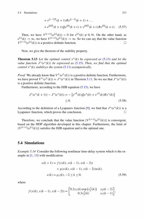
5.4 Simulations 213
+ v[i−1]T(k + 1)Rv[i−1](k + 1)+ . . .
+ e[0]T(k + i)Qe[0](k + i)+ v[0]T(k + i)Rv[0](k + i). (5.57)
Then, we have V [i+1](e[i](k)) > 0 for e[i](k) �= 0,∀i. On the other hand, ase[i](k) → ∞, we have V [i+1](e[i](k)) → ∞. So we can say that the value functionV [i+1](e[i](k)) is a positive definite function. �
Now, we give the theorem of the stability property.
Theorem 5.13 Let the optimal control v∗(k) be expressed as (5.13) and let thevalue function J ∗(e∗(k)) be expressed as (5.15). Then, we find that the optimalcontrol v∗(k) stabilizes the system (5.11) asymptotically.
Proof We already know that V L(eL(k)) is a positive definite function. Furthermore,we have proved V L(eL(k))= J ∗(e∗(k)) in Theorem 5.11. So we see that J ∗(e∗(k))is a positive definite function.
Furthermore, according to the HJB equation (5.15), we have
J ∗(e∗(k + 1))− J ∗(e∗(k))= −{e∗T(k)Qe∗(k)+ v∗T(k)Rv∗(k)
}
≤ 0. (5.58)
According to the definition of a Lyapunov function [9], we find that J ∗(e∗(k)) is aLyapunov function, which proves the conclusion. �
Therefore, we conclude that the value function {V [i+1](e[i](k))} is convergent,based on the HDP algorithm developed in this chapter. Furthermore, the limit of{V [i+1](e[i](k))} satisfies the HJB equation and is the optimal one.
5.4 Simulations
Example 5.14 Consider the following nonlinear time-delay system which is the ex-ample in [1, 13] with modification:
x(k + 1)= f (x(k), x(k − 1), x(k − 2))
+ g(x(k), x(k − 1), x(k − 2))u(k),
x(k)= �1(k),−2 ≤ k ≤ 0, (5.59)
where
f (x(k), x(k − 1), x(k − 2))=[
0.2x1(k) exp(x2
2(k))
x2(k − 2)0.3x2
2(k) x1(k − 1)
],
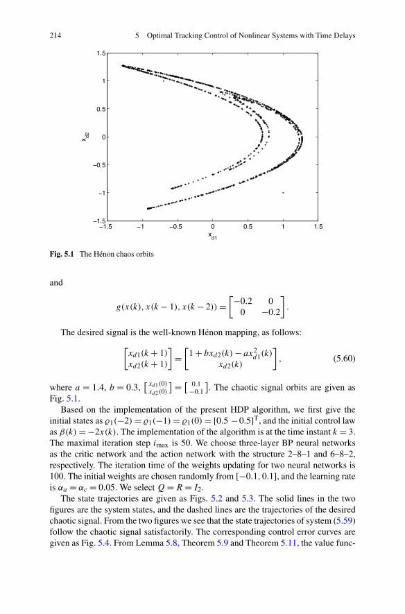
214 5 Optimal Tracking Control of Nonlinear Systems with Time Delays
Fig. 5.1 The Hénon chaos orbits
and
g(x(k), x(k − 1), x(k − 2))=[−0.2 0
0 −0.2
].
The desired signal is the well-known Hénon mapping, as follows:
[xd1(k + 1)xd2(k + 1)
]=[
1 + bxd2(k)− ax2d1(k)
xd2(k)
], (5.60)
where a = 1.4, b = 0.3,[ xd1(0)xd2(0)
] = [ 0.1−0.1
]. The chaotic signal orbits are given as
Fig. 5.1.Based on the implementation of the present HDP algorithm, we first give the
initial states as �1(−2)= �1(−1)= �1(0)= [0.5 −0.5]T, and the initial control lawas β(k)= −2x(k). The implementation of the algorithm is at the time instant k = 3.The maximal iteration step imax is 50. We choose three-layer BP neural networksas the critic network and the action network with the structure 2–8–1 and 6–8–2,respectively. The iteration time of the weights updating for two neural networks is100. The initial weights are chosen randomly from [−0.1,0.1], and the learning rateis αa = αc = 0.05. We select Q=R = I2.
The state trajectories are given as Figs. 5.2 and 5.3. The solid lines in the twofigures are the system states, and the dashed lines are the trajectories of the desiredchaotic signal. From the two figures we see that the state trajectories of system (5.59)follow the chaotic signal satisfactorily. The corresponding control error curves aregiven as Fig. 5.4. From Lemma 5.8, Theorem 5.9 and Theorem 5.11, the value func-
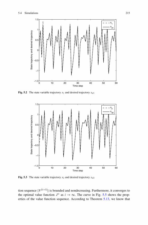
5.4 Simulations 215
Fig. 5.2 The state variable trajectory x1 and desired trajectory xd1
Fig. 5.3 The state variable trajectory x2 and desired trajectory xd2
tion sequence {V [i+1]} is bounded and nondecreasing. Furthermore, it converges tothe optimal value function J ∗ as i → ∞. The curve in Fig. 5.5 shows the prop-erties of the value function sequence. According to Theorem 5.13, we know that
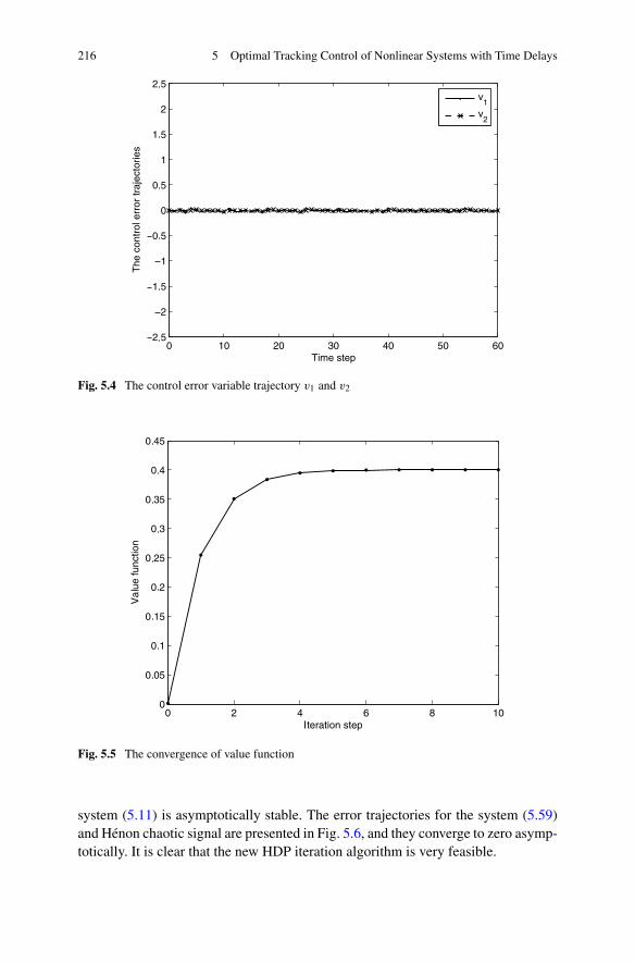
216 5 Optimal Tracking Control of Nonlinear Systems with Time Delays
Fig. 5.4 The control error variable trajectory v1 and v2
Fig. 5.5 The convergence of value function
system (5.11) is asymptotically stable. The error trajectories for the system (5.59)and Hénon chaotic signal are presented in Fig. 5.6, and they converge to zero asymp-totically. It is clear that the new HDP iteration algorithm is very feasible.
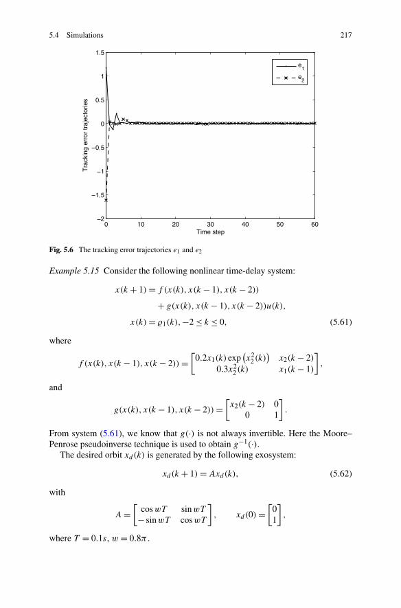
5.4 Simulations 217
Fig. 5.6 The tracking error trajectories e1 and e2
Example 5.15 Consider the following nonlinear time-delay system:
x(k + 1)= f (x(k), x(k − 1), x(k − 2))
+ g(x(k), x(k − 1), x(k − 2))u(k),
x(k)= �1(k),−2 ≤ k ≤ 0, (5.61)
where
f (x(k), x(k − 1), x(k − 2))=[
0.2x1(k) exp(x2
2(k))
x2(k − 2)0.3x2
2(k) x1(k − 1)
],
and
g(x(k), x(k − 1), x(k − 2))=[x2(k − 2) 0
0 1
].
From system (5.61), we know that g(·) is not always invertible. Here the Moore–Penrose pseudoinverse technique is used to obtain g−1(·).
The desired orbit xd(k) is generated by the following exosystem:
xd(k + 1)=Axd(k), (5.62)
with
A=[
coswT sinwT− sinwT coswT
], xd(0)=
[01
],
where T = 0.1s, w = 0.8π .
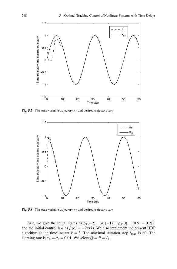
218 5 Optimal Tracking Control of Nonlinear Systems with Time Delays
Fig. 5.7 The state variable trajectory x1 and desired trajectory xd1
Fig. 5.8 The state variable trajectory x2 and desired trajectory xd2
First, we give the initial states as �1(−2) = �1(−1) = �1(0) = [0.5 − 0.2]T,and the initial control law as β(k) = −2x(k). We also implement the present HDPalgorithm at the time instant k = 3. The maximal iteration step imax is 60. Thelearning rate is αa = αc = 0.01. We select Q=R = I2.
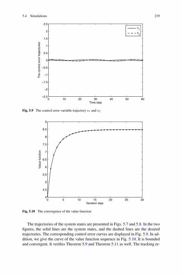
5.4 Simulations 219
Fig. 5.9 The control error variable trajectory v1 and v2
Fig. 5.10 The convergence of the value function
The trajectories of the system states are presented in Figs. 5.7 and 5.8. In the twofigures, the solid lines are the system states, and the dashed lines are the desiredtrajectories. The corresponding control error curves are displayed in Fig. 5.9. In ad-dition, we give the curve of the value function sequence in Fig. 5.10. It is boundedand convergent. It verifies Theorem 5.9 and Theorem 5.11 as well. The tracking er-
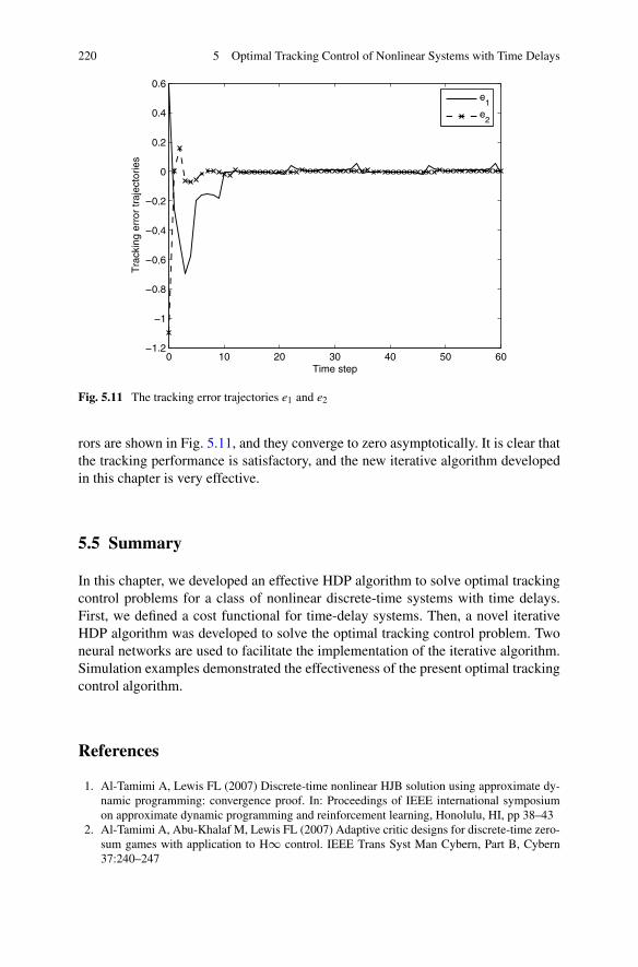
220 5 Optimal Tracking Control of Nonlinear Systems with Time Delays
Fig. 5.11 The tracking error trajectories e1 and e2
rors are shown in Fig. 5.11, and they converge to zero asymptotically. It is clear thatthe tracking performance is satisfactory, and the new iterative algorithm developedin this chapter is very effective.
5.5 Summary
In this chapter, we developed an effective HDP algorithm to solve optimal trackingcontrol problems for a class of nonlinear discrete-time systems with time delays.First, we defined a cost functional for time-delay systems. Then, a novel iterativeHDP algorithm was developed to solve the optimal tracking control problem. Twoneural networks are used to facilitate the implementation of the iterative algorithm.Simulation examples demonstrated the effectiveness of the present optimal trackingcontrol algorithm.
References
1. Al-Tamimi A, Lewis FL (2007) Discrete-time nonlinear HJB solution using approximate dy-namic programming: convergence proof. In: Proceedings of IEEE international symposiumon approximate dynamic programming and reinforcement learning, Honolulu, HI, pp 38–43
2. Al-Tamimi A, Abu-Khalaf M, Lewis FL (2007) Adaptive critic designs for discrete-time zero-sum games with application to H∞ control. IEEE Trans Syst Man Cybern, Part B, Cybern37:240–247
References 221
3. Al-Tamimi A, Lewis FL, Abu-Khalaf M (2008) Discrete-time nonlinear HJB solution usingapproximate dynamic programming: convergence proof. IEEE Trans Syst Man Cybern, PartB, Cybern 38:943–949
4. Ben-Israel A, Greville TNE (2002) Generalized inverse: theory and applications. Springer,New York
5. Chyung DH (1967) Discrete systems with time delay. Presented at the 5th annals Allertonconference on circuit and system theory, Urbana
6. Chyung DH (1968) Discrete optimal systems with time delay. IEEE Trans Autom Control13:117
7. Chyung DH, Lee EB (1966) Linear optimal systems with time delays. SIAM J Control4(3):548–575
8. Isidori A (2005) Nonlinear control systems II. Springer, Berlin9. Liao X, Wang L, Yu P (2007) Stability of dynamical systems. Elsevier, Amsterdam
10. Manu MZ, Mohammad J (1987) Time-delay systems analysis, optimization and applications.North-Holland, New York
11. Wei QL, Zhang HG, Liu DR, Zhao Y (2010) An optimal control scheme for a class of discrete-time nonlinear systems with time delays using adaptive dynamic programming. Acta AutomSin 36:121–129
12. Zhang HG, Song RZ (2011) Optimal tracking control for a class of nonlinear discrete-timesystems with time delays based on heuristic dynamic programming. IEEE Trans Neural Netw22(12):1851–1862
13. Zhang HG, Wei QL, Luo YH (2008) A novel infinite-time optimal tracking control schemefor a class of discrete-time nonlinear systems via the greedy HDP iteration algorithm. IEEETrans Syst Man Cybern, Part B, Cybern 38:937–942
Chapter 6Optimal Feedback Control for Continuous-TimeSystems via ADP
6.1 Introduction
In this chapter, we will study how to design a controller for continuous-time sys-tems via the ADP method. Although many ADP methods have been proposed forcontinuous-time systems [1, 6, 9, 10, 12, 13, 15, 17–19], a suitable frameworkin which the optimal controller can be designed for a class of unknown generalcontinuous-time systems is still not available. Therefore, in Sect. 6.2, we will de-velop a novel optimal robust feedback control scheme for a class of unknown gen-eral continuous-time systems using ADP method. The merit of present method isthat we require only the availability of input/output data instead of exact systemmodel. Moreover, the obtained control input can be guaranteed to be close to theoptimal control input within a small bound.
As is known, in the real world, many practical control systems are describedby nonaffine structure, such as chemical reactions, dynamic model in pendulumcontrol, etc. The difficulty associated with ADP for nonaffine nonlinear system isthat the nonlinear function is an implicit function with respect to the control variable.To overcome this difficulty, in Sect. 6.3, we will extend the ADP method to a classof nonaffine nonlinear systems. Through the present two methods, optimal controlproblems of a quite wide class of continuous-time nonlinear systems can be solved.
6.2 Optimal Robust Feedback Control for Unknown GeneralNonlinear Systems
In this section, a robust approximate optimal tracking control scheme is developedfor a class of unknown general nonlinear systems by using the ADP method. Inthe design of the controller, only available input/output data are required insteadof known system dynamics. First, a data-based model is established by a recurrentneural network (RNN) to reconstruct the unknown system dynamics using availableinput/output data. Then, based on the obtained data-based model, the ADP methodis utilized to design the approximate optimal tracking controller.
H. Zhang et al., Adaptive Dynamic Programming for Control,Communications and Control Engineering, DOI 10.1007/978-1-4471-4757-2_6,© Springer-Verlag London 2013
223
224 6 Optimal Feedback Control for Continuous-Time Systems via ADP
6.2.1 Problem Formulation
Consider the following general continuous-time nonlinear systems:
x(t)= f (x(t), u(t)), (6.1)
where x(t)= [x1(t), x2(t), . . . , xn(t)]T ∈ Rn is the state vector, u(t)= [u1(t), u2(t),
. . . , um(t)]T ∈ Rm is the input vector, and f (·, ·) is an unknown smooth nonlinear
function with respect to x(t) and u(t).In this section, our control objective is to design an optimal controller for (6.1),
which ensures that the state vector x(t) tracks the specified trajectory xd(t) whileminimizing the infinite-horizon cost functional as follows:
J (e(t), u)=∫ ∞
t
l(e(τ ), u(τ ))dτ, (6.2)
where e(t)= x(t)−xd(t) denotes the state tracking error, l(e(t), u(t))= eT(t)Qe(t)
+ uT(t)Ru(t) is the utility function, and Q and R are symmetric positive definitematrices with appropriate dimensions.
Since the system dynamics is completely unknown, we cannot apply existingADP methods to (6.1) directly. Therefore, it is now desirable to propose a novel con-trol scheme that does not need the exact system dynamics but only the input/outputdata which can be obtained during the operation of the system. Therefore, we pro-pose a data-based optimal robust tracking control scheme using ADP method forunknown general nonlinear continuous-time systems. Specifically, the design of thepresent controller is divided into two steps:
1. Establishing a data-based model based on an RNN by using available in-put/output data to reconstruct the unknown system dynamics, and
2. Designing the robust approximate optimal tracking controller based on the ob-tained data-based model
In the following, the establishment of the data-based model and the controllerdesign will be discussed in detail.
6.2.2 Data-Based Robust Approximate Optimal Tracking Control
Although we cannot obtain the exact system model in general, fortunately, we canaccess input–output data of the unknown general nonlinear systems in many prac-tical control processes. So it is desirable to use available input–output data in thedesign of the controller. The historical input–output data could be incorporated indi-rectly in the form of a data-based model. The data-based model could extract usefulinformation contained in the input–output data and capture input–output mapping.Markov models, neural network models, well structured filters, wavelet models, and
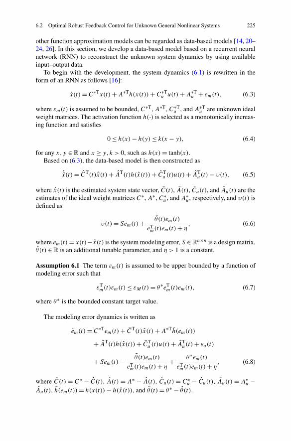
6.2 Optimal Robust Feedback Control for Unknown General Nonlinear Systems 225
other function approximation models can be regarded as data-based models [14, 20–24, 26]. In this section, we develop a data-based model based on a recurrent neuralnetwork (RNN) to reconstruct the unknown system dynamics by using availableinput–output data.
To begin with the development, the system dynamics (6.1) is rewritten in theform of an RNN as follows [16]:
x(t)= C∗Tx(t)+A∗Th(x(t))+C∗Tu u(t)+A∗T
u + εm(t), (6.3)
where εm(t) is assumed to be bounded, C∗T, A∗T, C∗Tu , and A∗T
u are unknown idealweight matrices. The activation function h(·) is selected as a monotonically increas-ing function and satisfies
0 ≤ h(x)− h(y)≤ k(x − y), (6.4)
for any x, y ∈R and x ≥ y, k > 0, such as h(x)= tanh(x).Based on (6.3), the data-based model is then constructed as
˙x(t)= CT(t)x(t)+ AT(t)h(x(t))+ CTu (t)u(t)+ AT
u(t)− υ(t), (6.5)
where x(t) is the estimated system state vector, C(t), A(t), Cu(t), and Au(t) are theestimates of the ideal weight matrices C∗, A∗, C∗
u , and A∗u, respectively, and υ(t) is
defined as
υ(t)= Sem(t)+ θ (t)em(t)
eTm(t)em(t)+ η
, (6.6)
where em(t)= x(t)− x(t) is the system modeling error, S ∈ Rn×n is a design matrix,
θ (t) ∈R is an additional tunable parameter, and η > 1 is a constant.
Assumption 6.1 The term εm(t) is assumed to be upper bounded by a function ofmodeling error such that
εTm(t)εm(t)≤ εM(t)= θ∗eT
m(t)em(t), (6.7)
where θ∗ is the bounded constant target value.
The modeling error dynamics is written as
em(t)= C∗Tem(t)+ CT(t)x(t)+A∗Th(em(t))
+ AT(t)h(x(t))+ CTu (t)u(t)+ AT
u(t)+ εa(t)
+ Sem(t)− θ (t)em(t)
eTm(t)em(t)+ η
+ θ∗em(t)eTm(t)em(t)+ η
, (6.8)
where C(t) = C∗ − C(t), A(t) = A∗ − A(t), Cu(t) = C∗u − Cu(t), Au(t) = A∗
u −Au(t), h(em(t))= h(x(t))− h(x(t)), and θ (t)= θ∗ − θ (t).
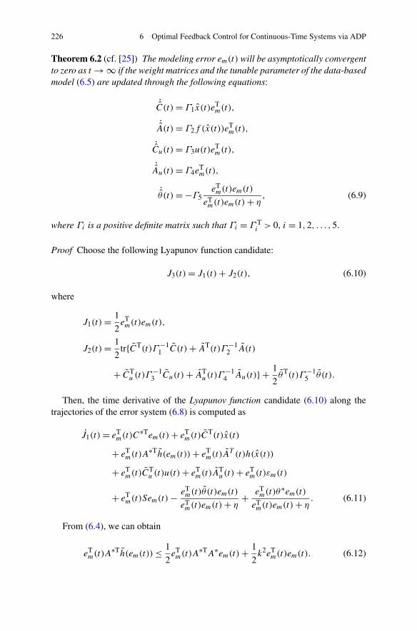
226 6 Optimal Feedback Control for Continuous-Time Systems via ADP
Theorem 6.2 (cf. [25]) The modeling error em(t) will be asymptotically convergentto zero as t → ∞ if the weight matrices and the tunable parameter of the data-basedmodel (6.5) are updated through the following equations:
˙C(t)= Γ1x(t)e
Tm(t),
˙A(t)= Γ2f (x(t))e
Tm(t),
˙Cu(t)= Γ3u(t)e
Tm(t),
˙Au(t)= Γ4e
Tm(t),
˙θ(t)= −Γ5
eTm(t)em(t)
eTm(t)em(t)+ η
, (6.9)
where Γi is a positive definite matrix such that Γi = Γ Ti > 0, i = 1,2, . . . ,5.
Proof Choose the following Lyapunov function candidate:
J3(t)= J1(t)+ J2(t), (6.10)
where
J1(t)= 1
2eTm(t)em(t),
J2(t)= 1
2tr{CT(t)Γ −1
1 C(t)+ AT(t)Γ −12 A(t)
+ CTu (t)Γ
−13 Cu(t)+ AT
u(t)Γ−1
4 Au(t)} + 1
2θT(t)Γ −1
5 θ (t).
Then, the time derivative of the Lyapunov function candidate (6.10) along thetrajectories of the error system (6.8) is computed as
J1(t)= eTm(t)C
∗Tem(t)+ eTm(t)C
T(t)x(t)
+ eTm(t)A
∗Th(em(t))+ eTm(t)A
T (t)h(x(t))
+ eTm(t)C
Tu (t)u(t)+ eT
m(t)ATu(t)+ eT
m(t)εm(t)
+ eTm(t)Sem(t)− eT
m(t)θ(t)em(t)
eTm(t)em(t)+ η
+ eTm(t)θ
∗em(t)eTm(t)em(t)+ η
. (6.11)
From (6.4), we can obtain
eTm(t)A
∗Th(em(t))≤ 1
2eTm(t)A
∗TA∗em(t)+ 1
2k2eT
m(t)em(t). (6.12)
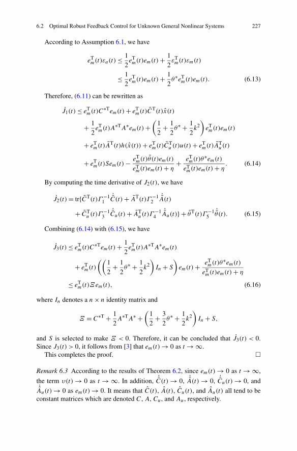
6.2 Optimal Robust Feedback Control for Unknown General Nonlinear Systems 227
According to Assumption 6.1, we have
eTm(t)εa(t)≤ 1
2eTm(t)em(t)+ 1
2εTm(t)εm(t)
≤ 1
2eTm(t)em(t)+ 1
2θ∗eT
m(t)em(t). (6.13)
Therefore, (6.11) can be rewritten as
J1(t)≤ eTm(t)C
∗Tem(t)+ eTm(t)C
T(t)x(t)
+ 1
2eTm(t)A
∗TA∗em(t)+(
1
2+ 1
2θ∗ + 1
2k2)eTm(t)em(t)
+ eTm(t)A
T(t)h(x(t))+ eTm(t)C
Tu (t)u(t)+ eT
m(t)ATu(t)
+ eTm(t)Sem(t)− eT
m(t)θ (t)em(t)
eTm(t)em(t)+ η
+ eTm(t)θ
∗em(t)eTm(t)em(t)+ η
. (6.14)
By computing the time derivative of J2(t), we have
J2(t)= tr{CT(t)Γ −11
˙C(t)+ AT(t)Γ −1
2˙A(t)
+ CTu (t)Γ
−13
˙Cu(t)+ AT
u(t)Γ−1
4˙Au(t)} + θT(t)Γ −1
5˙θ(t). (6.15)
Combining (6.14) with (6.15), we have
J3(t)≤ eTm(t)C
∗Tem(t)+ 1
2eTm(t)A
∗TA∗em(t)
+ eTm(t)
((1
2+ 1
2θ∗ + 1
2k2)In + S
)em(t)+ eT
m(t)θ∗em(t)
eTm(t)em(t)+ η
≤ eTm(t)Ξem(t), (6.16)
where In denotes a n× n identity matrix and
Ξ = C∗T + 1
2A∗TA∗ +
(1
2+ 3
2θ∗ + 1
2k2)In + S,
and S is selected to make Ξ < 0. Therefore, it can be concluded that J3(t) < 0.Since J3(t) > 0, it follows from [3] that em(t)→ 0 as t → ∞.
This completes the proof. �
Remark 6.3 According to the results of Theorem 6.2, since em(t) → 0 as t → ∞,
the term υ(t) → 0 as t → ∞. In addition, ˙C(t) → 0, ˙
A(t) → 0, ˙Cu(t) → 0, and
˙Au(t) → 0 as em(t) → 0. It means that C(t), A(t), Cu(t), and Au(t) all tend to beconstant matrices which are denoted C, A, Cu, and Au, respectively.
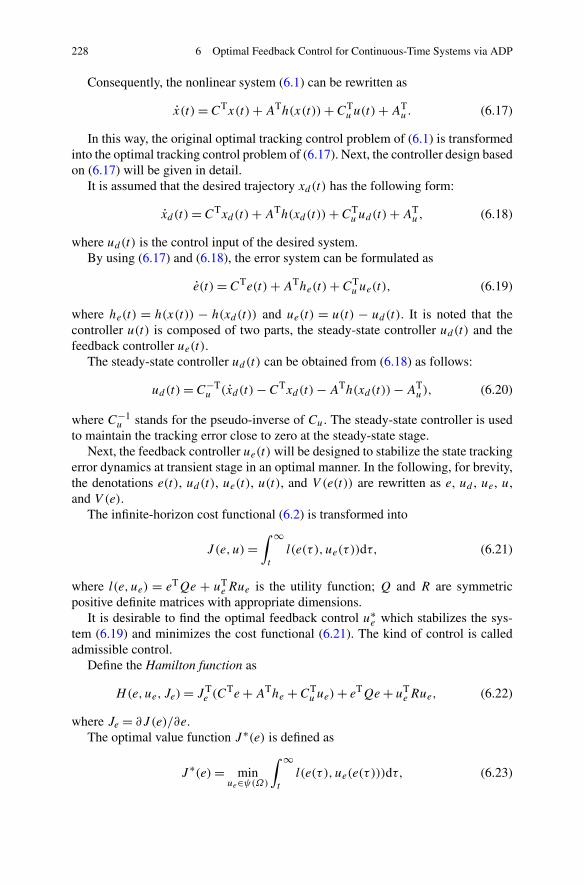
228 6 Optimal Feedback Control for Continuous-Time Systems via ADP
Consequently, the nonlinear system (6.1) can be rewritten as
x(t)= CTx(t)+ATh(x(t))+CTu u(t)+AT
u. (6.17)
In this way, the original optimal tracking control problem of (6.1) is transformedinto the optimal tracking control problem of (6.17). Next, the controller design basedon (6.17) will be given in detail.
It is assumed that the desired trajectory xd(t) has the following form:
xd (t)= CTxd(t)+ATh(xd(t))+CTu ud(t)+AT
u, (6.18)
where ud(t) is the control input of the desired system.By using (6.17) and (6.18), the error system can be formulated as
e(t)= CTe(t)+AThe(t)+CTu ue(t), (6.19)
where he(t) = h(x(t)) − h(xd(t)) and ue(t) = u(t) − ud(t). It is noted that thecontroller u(t) is composed of two parts, the steady-state controller ud(t) and thefeedback controller ue(t).
The steady-state controller ud(t) can be obtained from (6.18) as follows:
ud(t)= C−Tu (xd(t)−CTxd(t)−ATh(xd(t))−AT
u), (6.20)
where C−1u stands for the pseudo-inverse of Cu. The steady-state controller is used
to maintain the tracking error close to zero at the steady-state stage.Next, the feedback controller ue(t) will be designed to stabilize the state tracking
error dynamics at transient stage in an optimal manner. In the following, for brevity,the denotations e(t), ud(t), ue(t), u(t), and V (e(t)) are rewritten as e, ud , ue, u,and V (e).
The infinite-horizon cost functional (6.2) is transformed into
J (e,u)=∫ ∞
t
l(e(τ ), ue(τ ))dτ, (6.21)
where l(e, ue) = eTQe + uTe Rue is the utility function; Q and R are symmetric
positive definite matrices with appropriate dimensions.It is desirable to find the optimal feedback control u∗
e which stabilizes the sys-tem (6.19) and minimizes the cost functional (6.21). The kind of control is calledadmissible control.
Define the Hamilton function as
H(e,ue, Je)= J Te (C
Te+AThe +CTu ue)+ eTQe+ uT
e Rue, (6.22)
where Je = ∂J (e)/∂e.The optimal value function J ∗(e) is defined as
J ∗(e)= minue∈ψ(Ω)
∫ ∞
t
l(e(τ ), ue(e(τ )))dτ, (6.23)
6.2 Optimal Robust Feedback Control for Unknown General Nonlinear Systems 229
and satisfies
0 = minue∈ψ(Ω)
(H(e,ue, J∗e )). (6.24)
Further, we can obtain the optimal control u∗e by solving ∂H(e,ue, J
∗e )/∂ue = 0 as
u∗e = −1
2R−1CuJ
∗e , (6.25)
where J ∗e = ∂J ∗(e)/∂e. Then, the overall optimal control input can be rewritten as
u∗ = ud + u∗e .
In the following, we will focus on the optimal feedback controller design usingthe ADP method, which is implemented by employing the critic NN and the actionNN.
A neural network is utilized to approximate J (e) as
J (e)=WTc φc(e)+ εc, (6.26)
where Wc is the unknown ideal constant weights and φc(e) : Rn → RN1 is called
the critic NN activation function vector, N1 is the number of neurons in the hiddenlayer, and εc is the critic NN approximation error.
The derivative of the cost function J (e) with respect to e is
Je = �φTc Wc +�εc, (6.27)
where �φc � ∂φc(e)/∂e and �εc � ∂εc/∂e.Let Wc be an estimate of Wc, then we have the estimate of J (e) as follows:
J (e)= WTc φc(e). (6.28)
Then, the approximate Hamilton function can be derived as follows:
H(e,ue, Wa)= WTc �φc(CTe+AThe +CT
u ue)+ eTQe+ uTe Rue
= ec. (6.29)
Given any admissible control law ue, we desire to select Wc to minimize thesquared residual error Ec(Wc) as follows:
Ec(Wc)= 1
2eTc ec. (6.30)
The weight update law for the critic NN is a gradient descent algorithm, whichis given by
˙Wc = −αcσc(φ
Tc Wc + eTQe+ uT
e Rue), (6.31)
230 6 Optimal Feedback Control for Continuous-Time Systems via ADP
where αc > 0 is the adaptive gain of the critic NN, σc = σ/(σTσ + 1), σ =�φc(CTe + AThe + CT
u ue). Therefore, there exists a positive constant σcM > 1such that ‖σc‖ ≤ σcM . Define the weight estimation error of critic NN to beWc = Wc − Wc, and note that, for a fixed control law ue, the Hamilton function(6.22) becomes
H(e,ue,Wc)=WTc �φc(CTe+AThe +CT
u ue)+ eTQe+ uTe Rue
= εHJB, (6.32)
where the residual error due to the NN approximation error is εHJB = −�εc(CTe+AThe +CT
u ue).Rewriting (6.31) by using (6.32), we have
˙Wc = −αcσc(φ
Tc Wc + εHJB). (6.33)
To begin the development of the feedback control law, ue is approximated by theaction NN as
ue =WTa φa(e)+ εa, (6.34)
where Wa is the matrix of unknown ideal constant weights and φa(e) : Rn → RN2
is called the action NN activation function vector, N2 is the number of neurons inthe hidden layer, and εa is the action NN approximation error.
Let Wa be an estimate of Wa , the actual output can be expressed as
ue = WTa φa(e). (6.35)
The feedback error signal used for tuning action NN is defined to be the differ-ence between the real feedback control input applied to the error system (6.19) andthe desired control signal input minimizing (6.28) as
ea = WTa φa + 1
2R−1Cu�φT
c Wc. (6.36)
The objective function to be minimized by the action NN is defined as
Ea(Wa)= 1
2eTa ea. (6.37)
The weight update law for the action NN is a gradient descent algorithm, whichis given by
˙Wa = −αaφa
(WT
a φa + 1
2R−1Cu�φT
c Wc
)T
, (6.38)
where αa > 0 is the adaptive gain of the action NN.
6.2 Optimal Robust Feedback Control for Unknown General Nonlinear Systems 231
Define the weight estimation error of action NN to be Wa = Wa − Wa . Sincethe control law in (6.34) minimizes the infinite-horizon cost functional (6.26), from(6.25) we have
εa +WTa φa + 1
2R−1Cu�φT
c Wc + 1
2R−1Cu�εc = 0. (6.39)
Combining (6.38) with (6.39), we have
˙Wa = −αaφa
(WT
a φa + 1
2R−1Cu�φT
c Wc + ε12
)T
, (6.40)
where ε12 = −(εa +R−1Cu�εc/2).
Remark 6.4 It is important to note that the tracking error must be persistently ex-cited: enough for tuning the critic NN and action NN. In order to satisfy the persis-tent excitation condition, probing noise is added to the control input [17]. Further,the persistent excitation condition ensures ‖σc‖ ≥ σcm and ‖φa‖ ≥ φam with σcmand φam being positive constants.
Based on the above analysis, the optimal tracking controller is composed of thesteady-state controller ud and the optimal feedback controller ue . As a result, thecontrol input is written as
u= ud + ue. (6.41)
According to (6.35) and the error system (6.19), we have
e = CTe+AThe +CTu W
Ta φa. (6.42)
Subtracting and adding CTuWaφa to (6.42), and then recalling (6.34), (6.42) is
rewritten as
e = CTe+AThe +CTu W
Ta φa +CT
u ue −CTu εa. (6.43)
In the following, the stability analysis will be performed. First, the followingassumption is made, which can reasonably be satisfied under the current problemsettings.
Assumption 6.5
(a) The unknown ideal constant weights for the critic NN and the action NN, i.e.,Wc and Wa , are upper bounded so that ‖Wc‖ ≤ WcM and ‖Wa‖ ≤ WaM withWcM and WaM being positive constants, respectively.
(b) The NN approximation errors εc and εa are upper bounded so that ‖εc‖ ≤ εcMand ‖εa‖ ≤ εaM with εcM and εaM being positive constants, respectively.
(c) The vectors of the activation functions of the critic NN and the action NN, i.e.,φc and φa , are upper bounded so that ‖φc(·)‖ ≤ φcM and ‖φa(·)‖ ≤ φaM withφcM and φaM being positive constants, respectively.
232 6 Optimal Feedback Control for Continuous-Time Systems via ADP
(d) The gradients of the critic NN approximation error and the activation functionvector are upper bounded so that ‖�εc‖ ≤ ε′
cM and ‖�φa‖ ≤ φdM with ε′cM
and φdM being positive constants. The residual error is upper bounded so that‖εHJB‖ ≤ εHJBM with εHJBM being positive constant.
Now we are ready to prove the following theorem.
Theorem 6.6 (cf. [25]) Consider the system given by (6.17) and the desired trajec-tory (6.18). Let the control input be provided by (6.41). The weight updating laws ofthe critic NN and the action NN are given by (6.31) and (6.38), respectively. Let theinitial action NN weights be chosen to generate an initial admissible control. Then,the tracking error e, the weight estimate errors Wc and Wa are uniformly ultimatelybounded (UUB) with the bounds specifically given by (6.51)–(6.53). Moreover, theobtained control input u is close to the optimal control input u∗ within a small boundεu, i.e., ‖u− u∗‖ ≤ εu as t → ∞ for a small positive constant εu.
Proof Choose the following Lyapunov function candidate:
L(t)= L1(t)+L2(t)+L3(t), (6.44)
where L1(t) = tr{WTc Wc}/2αc, L2(t) = αc tr{WT
a Wa}/2αa , and L3(t) =αcαa(e
Te+ Γ J(e)) with Γ > 0.According to Assumption 6.5 and using (6.21), (6.33), and (6.40), the time
derivative of the Lyapunov function candidate (6.44) along the trajectories of theerror system (6.43) is computed as follows:
L(t)= L1(t)+ L2(t)+ L3(t), (6.45)
where
L1(t)= 1
αctr{WT
c˙Wc}
= 1
αctr{WT
c (−αcσc(φTc Wc + εHJB))}
≤ −(σ 2cm − αc
2σ 2cM
)‖Wc‖2 + 1
2αcε2
HJB,
L2(t)= αc
αatr{WT
a˙Wa}
= αc
αatr
{WT
a
(−αaφa
(WT
a φa + 1
2R−1Cu�φT
c Wc + ε12
)T)}
≤ −(αcφ
2am − 3
4αcαaφ
2aM
)‖Wa‖2
+ αc
4αa‖R−1‖2‖Cu‖2φ2
dM‖Wc‖2 + αc
2αaεT
12ε12,
6.2 Optimal Robust Feedback Control for Unknown General Nonlinear Systems 233
L3(t)= 2αcαaeTe+ αcαaΓ (−eTQe− uT
e Rue)
= 2αcαaeT(CTe+AT he +CT
u WTa φa +CT
u ue
−CTu εa)+ αcαaΓ (−eTQe− uT
e Rue)
≤ αcαa(2‖C‖ + 3 + ‖A‖2 + k2 − Γ λmin(Q))‖e‖2
+ αcαaφ2aM‖Cu‖2‖Wa‖2 + αcαa‖Cu‖2εT
a εa
+ αcαa(‖Cu‖2 − Γ λmin(R))‖ue‖2.
Then we obtain
L(t)≤ −(σ 2cm − αc
2σ 2cM − αc
4αa‖R−1‖2‖Cu‖2φ2
dM
)‖Wc‖2
−(αcφ
2am − 3
4αcαaφ
2aM − αcαaφ
2aM‖Cu‖2
)‖Wa‖2
− αcαa(−‖Cu‖2 + Γ λmin(R))‖ue‖2
− αcαa(−2‖C‖ − 3 − ‖A‖2 − k2 + Γ λmin(Q))‖e‖2
+ 1
2αcε2
HJB + αc
2αaεT
12ε12 + αcαa‖Cu‖2εTa εa. (6.46)
By using Assumption 6.5, we have ‖ε12‖ ≤ ε12M , where ε12M = εaM +R−1Cuε
′cM/2. Then, we have
1
2αcε2
HJB + αc
2αaεT
12ε12 + αcαa‖Cu‖2εT12ε12 ≤DM, (6.47)
where DM = ε2HJBM/(2αc)+ αcε
212M/(2αa)+ αcαa‖Cu‖2ε2
12M .If Γ , αc , and αa are selected to satisfy
Γ > max
{ ‖Cu‖2
λmin(R),
2‖C‖ + 3 + ‖A‖2 + k2
λmin(Q)
}, (6.48)
αc <4αaσ 2
cm
2αaσ 2cM + ‖R−1‖2‖Cu‖2φ2
dM
, (6.49)
αa <4φ2
am
3φ2aM + 4φ2
aM‖Cu‖2, (6.50)
and given the following inequalities:
‖e‖>√
DM
αcαa(−2‖C‖ − 3 − ‖A‖2 − k2 + Γ λmin(Q))
� be, (6.51)
234 6 Optimal Feedback Control for Continuous-Time Systems via ADP
or
‖Wc‖>√
4αaDM
4αaσ 2cm − 2αaαcσ 2
cM − αc‖R−1‖2‖Cu‖2φ2dM
� bWc, (6.52)
or
‖Wa‖>√
4DM
4αcφ2am − 3αcαaφ2
aM − 4αcαaφ2aM‖Cu‖2
� bWa, (6.53)
then we can conclude L(t) < 0. Therefore, using Lyapunov theory [7], it can beconcluded that the tracking error e, and the NN weight estimation errors Wc and Wa
are UUB.Next, we will prove ‖u − u∗‖ ≤ εu as t → ∞. Recalling the expression of u∗
together with (6.34) and (6.41), we have
u− u∗ = WTa φa + εa. (6.54)
When t → ∞, the upper bound of (6.54) is
‖u− u∗‖ ≤ εu, (6.55)
where εu = bWaφaM + εaM .
This completes the proof. �
Remark 6.7 From (6.31) and (6.38), it is noted that the weights of critic NN andaction NN are updated simultaneously in contrast with some standard ADP methodsin which the weights of critic NN and action NN are updated sequentially.
Remark 6.8 If the NN approximation errors εc and εa are considered to be neg-ligible, then from (6.47) we have DM = 0, with u → u∗. Otherwise, the obtainedcontrol input u is close to the optimal input u∗ within a small bound εu.
Due to the presence of the NN approximation errors εc and εa , the tracking erroris UUB instead of asymptotically convergent to zero. In the following, for improvingthe tracking performance, an additional robustifying term is developed to attenuatethe NN approximation errors such that tracking error converges to zero asymptoti-cally, which can be constructed in the form
ur = Kre
eTe+ ζ, (6.56)
where ζ > 0 is a constant, Kr > Kr min is a designed parameter. Kr min is selectedto satisfy the following inequality:
Kr min ≥ DM(eTe+ ζ )
2αcαa‖Cu‖eTe. (6.57)
6.2 Optimal Robust Feedback Control for Unknown General Nonlinear Systems 235
Then, the overall control input is given as
uad = u− ur, (6.58)
where u is the same as (6.41).Applying (6.58) to the error system (6.17) and using (6.18), a new error system
is obtained as follows:
e = CTe+AThe +CTu W
Ta φa +CT
u ue −CTu εa −CT
u ur . (6.59)
Theorem 6.9 (cf. [25]) Consider the system given by (6.17) and the desired trajec-tory (6.18). Let the control input be provided by (6.58). The weight updating laws ofthe critic NN and the action NN are given by (6.31) and (6.38), respectively. Let theinitial action NN weights be chosen to generate an initial admissible control. Then,the tracking error e and the weight estimation errors Wc and Wa will asymptoticallyconverge to zero. Moreover, the obtained control input uad is close to the optimalcontrol input u∗ within a small bound δu, i.e., ‖uad − u∗‖ ≤ δu as t → ∞ for asmall positive constant δu.
Proof Choose the same Lyapunov function candidate as that in Theorem 6.6. Dif-ferentiating the Lyapunov function candidate in (6.44) along the trajectories of theerror system in (6.59), similar to the proof of Theorem 6.6, by using (6.56) and(6.57), we obtain
L(t)≤ −(σ 2cm − αc
2σ 2cM − αc
4αa‖R−1‖2‖Cu‖2φ2
dM
)‖Wc‖2
−(αcφ
2am − 3
4αcαaφ
2aM − αcαaφ
2aM‖Cu‖2
)‖Wa‖2
− αcαa(−‖Cu‖2 + Γ λmin(R))‖ue‖2
− αcαa(−2‖C‖ − 3 − ‖A‖2 − k2 + Γ λmin(Q))‖e‖2. (6.60)
Choosing Γ , αc, and αa as Theorem 6.6, we have L(t)≤ 0. Equations (6.44) and(6.60) guarantee that the tracking error e, NN weight estimation errors Wc and Wa
are bounded, since L is nonincreasing. Because all the variables on the right-handside of (6.59) are bounded, e is also bounded. From (6.60), we have
L(t)≤ −Be‖e‖2, (6.61)
where Be = αcαa(−2‖C‖ − 3 − ‖A‖2 − k2 + Γ λmin(Q)).Integrating both sides of (6.61) and after some manipulations, we have
∫ ∞
0‖e‖2dt ≤ B−1
e (L(0)−L(∞)). (6.62)
Since the right side of (6.59) is bounded, ‖e‖ ∈ L2. Using Barbalat’s lemma [7],we have limt→∞ ‖e‖ = 0. Similarly, we can prove that limt→∞ ‖Wc‖ = 0 andlimt→∞ ‖Wa‖ = 0.
236 6 Optimal Feedback Control for Continuous-Time Systems via ADP
Next, we will prove ‖uad − u∗‖ ≤ δu as t → ∞. From (6.34) and (6.58), we canhave
uad − u∗ = WTa φa + εa + ur . (6.63)
Since ‖e‖ → 0 as t → ∞, the robustifying control input ‖ur‖ → 0 as t → ∞.Then, the upper bound of (6.63) is
‖uad − u∗‖ ≤ δu, (6.64)
where δu = εaM .This completes the proof. �
Remark 6.10 From (6.55) and (6.64), it can be seen that δu is smaller than εu, whichreveals the role of the robustifying term in making the obtained control input closerto the optimal control input.
6.2.3 Simulations
In this subsection, two examples are provided to demonstrate the effectiveness ofthe present approach.
Example 6.11 Consider the following affine nonlinear continuous-time system:
x1 = −x1 + x2,
x2 = −0.5x1 − 0.5x2(1 − (cos(2x1)+ 2)2)
+ (cos(2x1)+ 2)u. (6.65)
The cost functional is defined by (6.21) where Q and R are chosen as identitymatrices of appropriate dimensions. The control object is to make x1 follow thedesired trajectory x1d = sin(t). It is assumed that the system dynamics is unknownand input/output data are available.
First, a data-based model is established to estimate the nonlinear system dy-namics. Let us select the RNN as (6.5) with S = −30I2 and η = 1.5. The ac-tivation function h(x) is selected as hyperbolic tangent function tanh(x). Selectthe design parameters in Theorem 6.2 as Γ1 = [1,0.1;0.1,1], Γ2 = [1,0.2;0.2,1],Γ3 = [1,0.1;0.1,1], Γ4 = 0.2, and Γ5 = 0.1. Then, we can obtain the trajectories ofthe modeling error as shown in Fig. 6.1. It is observed that the obtained data-basedmodel can reconstruct the nonlinear system dynamics successfully, as Theorem 6.2predicted.
Then, based on the obtained data-based model, the approximate optimal robustcontroller is implemented for the unknown affine nonlinear continuous-time system(6.65). The activation function of the critic NN is selected as φc = [e2
1 e1e2 e22]T, the
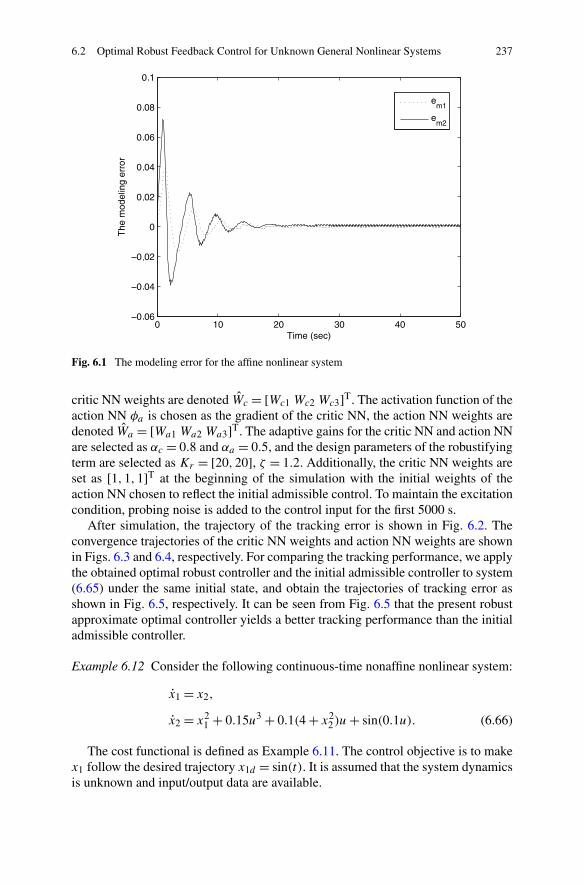
6.2 Optimal Robust Feedback Control for Unknown General Nonlinear Systems 237
Fig. 6.1 The modeling error for the affine nonlinear system
critic NN weights are denoted Wc = [Wc1 Wc2 Wc3]T. The activation function of theaction NN φa is chosen as the gradient of the critic NN, the action NN weights aredenoted Wa = [Wa1 Wa2 Wa3]T. The adaptive gains for the critic NN and action NNare selected as αc = 0.8 and αa = 0.5, and the design parameters of the robustifyingterm are selected as Kr = [20,20], ζ = 1.2. Additionally, the critic NN weights areset as [1,1,1]T at the beginning of the simulation with the initial weights of theaction NN chosen to reflect the initial admissible control. To maintain the excitationcondition, probing noise is added to the control input for the first 5000 s.
After simulation, the trajectory of the tracking error is shown in Fig. 6.2. Theconvergence trajectories of the critic NN weights and action NN weights are shownin Figs. 6.3 and 6.4, respectively. For comparing the tracking performance, we applythe obtained optimal robust controller and the initial admissible controller to system(6.65) under the same initial state, and obtain the trajectories of tracking error asshown in Fig. 6.5, respectively. It can be seen from Fig. 6.5 that the present robustapproximate optimal controller yields a better tracking performance than the initialadmissible controller.
Example 6.12 Consider the following continuous-time nonaffine nonlinear system:
x1 = x2,
x2 = x21 + 0.15u3 + 0.1(4 + x2
2)u+ sin(0.1u). (6.66)
The cost functional is defined as Example 6.11. The control objective is to makex1 follow the desired trajectory x1d = sin(t). It is assumed that the system dynamicsis unknown and input/output data are available.
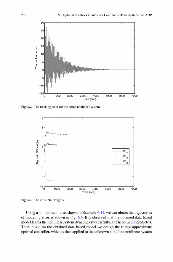
238 6 Optimal Feedback Control for Continuous-Time Systems via ADP
Fig. 6.2 The tracking error for the affine nonlinear system
Fig. 6.3 The critic NN weights
Using a similar method as shown in Example 6.11, we can obtain the trajectoriesof modeling error as shown in Fig. 6.6. It is observed that the obtained data-basedmodel learns the nonlinear system dynamics successfully, as Theorem 6.2 predicted.Then, based on the obtained data-based model we design the robust approximateoptimal controller, which is then applied to the unknown nonaffine nonlinear system
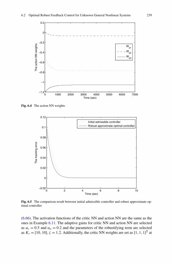
6.2 Optimal Robust Feedback Control for Unknown General Nonlinear Systems 239
Fig. 6.4 The action NN weights
Fig. 6.5 The comparison result between initial admissible controller and robust approximate op-timal controller
(6.66). The activation functions of the critic NN and action NN are the same as theones in Example 6.11. The adaptive gains for critic NN and action NN are selectedas αc = 0.5 and αa = 0.2 and the parameters of the robustifying term are selectedas Kr = [10,10], ζ = 1.2. Additionally, the critic NN weights are set as [1,1,1]T at
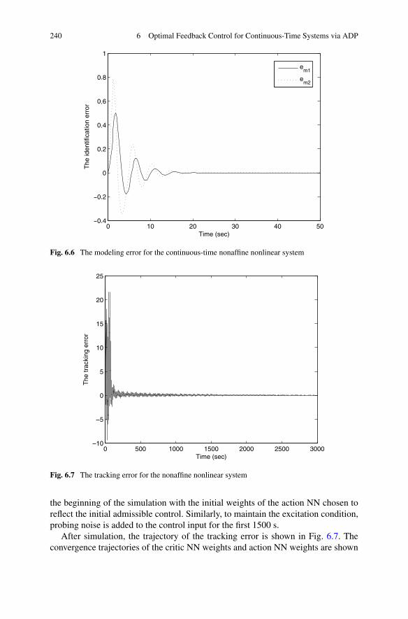
240 6 Optimal Feedback Control for Continuous-Time Systems via ADP
Fig. 6.6 The modeling error for the continuous-time nonaffine nonlinear system
Fig. 6.7 The tracking error for the nonaffine nonlinear system
the beginning of the simulation with the initial weights of the action NN chosen toreflect the initial admissible control. Similarly, to maintain the excitation condition,probing noise is added to the control input for the first 1500 s.
After simulation, the trajectory of the tracking error is shown in Fig. 6.7. Theconvergence trajectories of the critic NN weights and action NN weights are shown
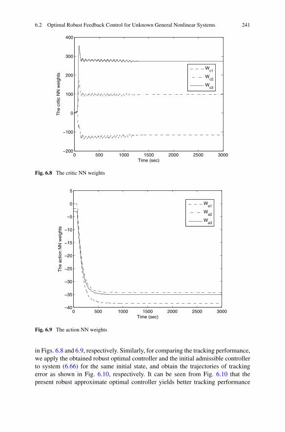
6.2 Optimal Robust Feedback Control for Unknown General Nonlinear Systems 241
Fig. 6.8 The critic NN weights
Fig. 6.9 The action NN weights
in Figs. 6.8 and 6.9, respectively. Similarly, for comparing the tracking performance,we apply the obtained robust optimal controller and the initial admissible controllerto system (6.66) for the same initial state, and obtain the trajectories of trackingerror as shown in Fig. 6.10, respectively. It can be seen from Fig. 6.10 that thepresent robust approximate optimal controller yields better tracking performance
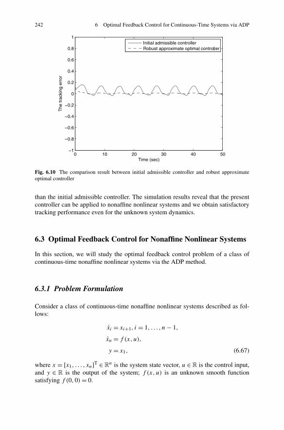
242 6 Optimal Feedback Control for Continuous-Time Systems via ADP
Fig. 6.10 The comparison result between initial admissible controller and robust approximateoptimal controller
than the initial admissible controller. The simulation results reveal that the presentcontroller can be applied to nonaffine nonlinear systems and we obtain satisfactorytracking performance even for the unknown system dynamics.
6.3 Optimal Feedback Control for Nonaffine Nonlinear Systems
In this section, we will study the optimal feedback control problem of a class ofcontinuous-time nonaffine nonlinear systems via the ADP method.
6.3.1 Problem Formulation
Consider a class of continuous-time nonaffine nonlinear systems described as fol-lows:
xi = xi+1, i = 1, . . . , n− 1,
xn = f (x,u),
y = x1, (6.67)
where x = [x1, . . . , xn]T ∈ Rn is the system state vector, u ∈ R is the control input,
and y ∈ R is the output of the system; f (x,u) is an unknown smooth functionsatisfying f (0,0)= 0.
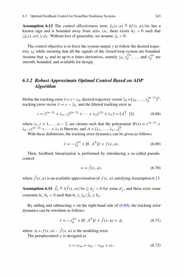
6.3 Optimal Feedback Control for Nonaffine Nonlinear Systems 243
Assumption 6.13 The control effectiveness term fu(x,u) � ∂f (x,u)/∂u has aknown sign and is bounded away from zero, i.e., there exists df > 0 such that|fu(x,u)| ≥ df . Without loss of generality, we assume fu > 0.
The control objective is to force the system output y to follow the desired trajec-tory yd while ensuring that all the signals of the closed-loop system are bounded.Assume that yd and its up to n times derivatives, namely yd , y
(2)d , . . . , and y
(n)d are
smooth, bounded, and available for design.
6.3.2 Robust Approximate Optimal Control Based on ADPAlgorithm
Define the tracking error y=y−yd , desired trajectory vector yd=[yd, . . . , y(n−1)d ]T,
tracking error vector x = x − yd , and the filtered tracking error as
r = y(n−1) + λn−1y(n−2) + · · · + λ2y
(1) + λ1y = [ΛT 1]x, (6.68)
where λi, i = 1, . . . , n − 2, are chosen such that the polynomial H(s) = s(n−1) +λn−1s
(n−2) + · · · + λ1 is Hurwitz, and Λ= [λ1, . . . , λn−1]T.With these definitions, the tracking error dynamics can be given as follows:
r = −y(n)d + [0 ΛT]x + f (x,u). (6.69)
Then, feedback linearization is performed by introducing a so-called pseudo-control
υ = f (x, u), (6.70)
where f (x, u) is an available approximation of f (x,u) satisfying Assumption 6.13.
Assumption 6.14 fu � ∂f (x,u)/∂u ≥ df> 0 for some d
f, and there exist some
constants bl , bu > 0 such that bl ≤ fu/fu ≤ bu.
By adding and subtracting υ on the right-hand side of (6.69), the tracking errordynamics can be rewritten as follows:
r = −y(n)d + [0 ΛT]x + f (x, u)+Δ, (6.71)
where Δ= f (x,u)− f (x, u) is the modeling error.The pseudocontrol υ is designed as
υ = υrm + υdc − υad + υr, (6.72)
244 6 Optimal Feedback Control for Continuous-Time Systems via ADP
where υrm = y(n)d −[0 ΛT]x, υdc = −Kr is to stabilize the tracking error dynamics
in the absence of a modeling error, υad is used to approximately cancel the modelingerror, and υr is a robustifying term.
By inverting (6.70), we have the following control law:
u= f−1(x,υ). (6.73)
Then, applying (6.73) to (6.71), we have
r = −Kr +Δ− υad + υr . (6.74)
The term Δ− υad can be expressed as
Δ− υad = f (x, f−1(x,υrm + υdc − υad + υr))− υrm − υdc − υr . (6.75)
Reference [2] points out that Δ depends on υad through (6.72) and (6.73), whileυad is designed to cancel Δ. A contraction mapping assumption on Δ with respectto υad is required to guarantee the existence of a smooth function υ∗
ad =Δ(·, υ∗ad).
To remove the contraction mapping assumption, we follow the work of [8]. Defineυl � υrm + υdc, υ∗ � f (x, f−1(x,υl)). Then we have υl = f (x, f−1(x,υ∗)).
Using the mean value theorem [5], (6.75) can be expressed as
Δ− υad = f (x,u)− f (x, u)− υad
= f (x, f−1(x,υ))− υl + υad − υr − υad
= f (x, f−1(x,υ))− f (x, f−1(x,υ∗))− υr
= fυ(υ)(υ − υ∗)− υr
= fυ(υ)(υl − υad + υr − f (x, f−1(x,υl)))− υr
= fυ(υ)(−υad + υr + Δ)− υr, (6.76)
where Δ = υl − f (x, f−1(x,υl)) = f (x, f−1(x,υ∗)) − f (x,f−1(x,υl)) de-notes the unknown uncertain term, fυ(υ) � (∂f/∂u)(∂u/∂v)|υ=υ = (∂f/∂u)/
(∂f /∂u)|u=f−1(x,υ)
, υ = λυ + (1 − λ)υ∗ and 0 ≤ λ(υ)≤ 1.Then, substituting (6.76) into (6.74), we have
r = −Kr + fυ(υ)(−υad + Δ)+ fυ(υ)υr . (6.77)
If Δ is known, υad can be chosen as υad = Δ; then we let υr = 0. Since Δ isunknown, the desired υad cannot be implemented directly. Instead, an action NN isemployed to approximate Δ as follows:
Δ=WTa φa(x)+ εa(x), (6.78)
where x = [1, x,υl, yd ], Wa ∈ RN is the ideal weight of the action NN, φa(x) ∈ R
N
is the basis function of the action NN, and εa(x) is the reconstruction error of theaction NN satisfying ‖εa(x)‖ ≤ ε∗
a .
6.3 Optimal Feedback Control for Nonaffine Nonlinear Systems 245
Remark 6.15 Because the unknown nonlinear function f (x,u) of (6.67) is an im-plicit function with respect to the control input u, traditional ADP methods canrarely be applied. To overcome this difficulty, the action NN is employed to ap-proximate the derived unknown uncertain term Δ instead of modeling the unknownsystem (6.67) directly.
The adaptive signal υad is designed as
υad = WTa φa(x), (6.79)
where Wa is the estimate of Wa .Substituting (6.78) and (6.79) into (6.77), the following is immediate:
r = −Kr + (fυ(υ)− bu)WTa φa(x)+ buW
Ta φa
+ fυ(υ)υr + fυ(υ)εa(x), (6.80)
where Wa =Wa − Wa .Using adaptive bounding technique, the robustifying term υr is designed as
υr = − br
1 − br|κ|ψ tanh
(Rψ
α
), (6.81)
where br = 1− (bl/bu) < 1 and α is a design parameter, κ is the adaptive parameter,R and ψ will be defined later. Applying (6.81) to (6.80), the tracking error dynamicscan be rewritten as
r = −Kr + buWTa φa + bu
[υr +
(fυ(υ)
bu− 1
)(υr + WT
a φa
)]
+ fυ(υ)εa(x). (6.82)
Remark 6.16 Since tanh(·) can maintain a continuous control signal while sgn(·)will result in a chattering phenomenon due to its discontinuity, the robustifying termis designed based on tanh(·) rather than sgn(·).
Next, we choose the critic signal as [13]
Rn = R+ |R|WTc φc(r). (6.83)
The first term R is called the primary critic signal which is defined in terms of theperformance measure as
R= χ
1 + e−mr− χ
1 + emr, (6.84)
where m is a positive constants and the value of R is bounded in the interval[−χ,χ] with χ > 0 being the critic slope gain. The second term |R|WT
c φc(r) is
246 6 Optimal Feedback Control for Continuous-Time Systems via ADP
called the second critic signal, where Wc is the ideal weight of critic NN and φc(r)
is the basis function of critic NN. The actual output of the critic NN is WTc φc(r)
where Wc is the estimate of Wc. Then, the actual critic signal can be expressed asRn = R + |R|WT
c φc(r). Define Wc = Wc − Wc. It should be noted that R willapproach zero when r approaches zero. Therefore we can conclude that Rn willapproach zero. As a learning signal, the critic signal Rn is more informative thanthe filtered tracking error r . Consequently, a larger control input can be yielded andbetter tracking performance can be obtained.
Next, the uniformly ultimate boundedness of the closed-loop system is demon-strated by the Lyapunov method.
Assumption 6.17 The ideal weights of the action NN and the critic NN, i.e., Wa
and Wc, are bounded above by unknown positive constants so that ‖Wa‖ ≤ W ∗a ,
‖Wc‖ ≤W ∗c .
Assumption 6.18 The activation functions of the action NN and critic NN, φaand φc , are bounded above by known positive constants, so that ‖φa‖ ≤ φ∗
a ,‖φc‖ ≤ φ∗
c .
Lemma 6.19 (cf. [4]) The following inequality holds:
‖δ‖� ‖Rfυ(υ)εa(x)+ bubr |R|‖Wa‖‖φa‖+ bu|R|tr{WT
a φaφTc Wa −WT
a φa(φTc Wc)}‖
≤ bubr |R|κ∗ψ, (6.85)
where κ∗ is an unknown constant and ψ = 1 + ‖Wa‖ + ‖Wc‖.
Proof Using Assumptions 6.13, 6.14, 6.17, and 6.18, the boundedness of εa(x) andthe inequality ‖Wa‖ ≤ ‖Wa‖ + ‖W ∗
a ‖, we have
‖δ‖ ≤ |R|buε∗a + bubr |R|‖Wa‖‖φa‖ + bubr |R|W ∗
a ‖φa‖+ bu|R|φ∗
aφ∗cW
∗c ‖Wa‖ + bu|R|φ∗
aφ∗cW
∗a ‖Wc‖
≤ bubr |R|κ∗ψ, (6.86)
where κ∗ � max{ε∗a/br +W ∗
a φ∗a ,φ
∗a (1+φ∗
cW∗c /br),φ
∗aφ
∗cW
∗a /br}, ψ = 1+‖Wa‖+
‖Wc‖.This completes the proof. �
Theorem 6.20 (cf. [4]) Under Assumptions 6.13, 6.14 and 6.17, considering theclosed-loop system consisting of system (6.67) and the control u provided by (6.73),the weights tuning laws of the action NN and critic NN are
˙Wa = α1(φa(R+ |R|WT
c φc)T −KWa |R|Wa), (6.87)
6.3 Optimal Feedback Control for Nonaffine Nonlinear Systems 247
˙Wc = −α2(|R|φc(WT
a φa)T +KWc |R|Wc), (6.88)
and the tuning law of the adaptive parameter is
˙κ = α3
(Rψ tanh
(Rψ
α
)−Kκκ
), (6.89)
where α1, α2, α3, KWa , KWc , and Kκ are the positive design parameters. If Kκ >
1/(bubr), then all the closed-loop signals are uniformly ultimately bounded.
Proof Choose a Lyapunov function candidate as
L= ρ(r)+ bu
2α1tr{WT
a Wa} + bu
2α2tr{WT
c Wc} + bubr
2α3κ2, (6.90)
where ρ(r) = χ(ln(1 + emr)+ ln(1 + e−mr))/m, κ = κ∗ − κ . The time derivativeof (6.90) can be expressed as
L= Rr + bu
α1tr{WT
a˙Wa} + bu
α2tr{WT
c˙Wc} + bubr
α3κ ˙κ. (6.91)
Substituting (6.82) into (6.91), we have
L= R{−Kr + buW
Ta φa + bu
[υr +
(fυ(υ)
bu− 1
)(fυ(υ)+ WT
a φa
)]}
+Rfυ(υ)εa(x)+ bu
α1tr{WT
a˙Wa} + bu
α2tr{WT
c˙Wc} + bubr
α3κ ˙κ. (6.92)
Applying (6.87) to (6.92), we have
L= R{−Kr + buW
Ta φa + bu
[υr +
(fυ(υ)
bu− 1
)(fυ(υ)+ WT
a φa
)]}
+Rfυ(υ)εa(x)− butr{WT
a (φa(R+ |R|WTc φc)
T −KWa |R|Wa)}
+ bu
α2tr{WT
c˙Wc} + bubr
α3κ ˙κ. (6.93)
Due to the fact that
butr{WTa φaR} = RbuW
Ta φa,
tr{WTa φa|R|(WT
c φc)T} = |R|WT
a φaφTc Wc
= |R|(−WTa φaφ
Tc Wa +WT
a φaφTc Wc + WT
a φaφTc Wc),
(6.94)
248 6 Optimal Feedback Control for Continuous-Time Systems via ADP
and using (6.88), (6.93) can be rewritten as
L≤ −RKr +Rbu
[υr +
(fυ(υ)
bu− 1
)(fυ(υ)+ WT
a φa
)]+Rfυ(υ)εa(x)
+ buKWa |R|tr{WTa Wa} + buKWc |R|tr{WT
c Wc}
+ bu|R|(−WTa φa(φ
Tc Wa)+WT
a φaφTc Wc)+ bubr
α3κ ˙κ. (6.95)
With the robustifying term in (6.81), we have
Rυr = − br
1 − br|κ|Rψsgn(Rψ)+ br
1 − br|κ|
(|Rψ | −Rψ tanh
(Rψ
α
)).
(6.96)
According to Assumptions 6.13 and 6.14, we have
∣∣∣∣
(fυ(υ)
bu− 1
)(υr + WT
a φa
)∣∣∣∣≤ br |υr | + br‖Wa‖‖φa‖. (6.97)
Substituting (6.96) and (6.97) into (6.95), we have
L≤ −RKr + bu
[− br
1 − br|κ|Rψsgn(Rψ)+ brR|υr |
+ br
1 − br|κ|
(|Rψ | −Rψ tanh
(Rψ
α
))]
+ buKWa |R|tr{WTa Wa} + buKWc |R|tr{WT
c Wc}
+ δ + bubr
α3κ ˙κ. (6.98)
According to Lemma 6.19 and the inequality 0 ≤ |Rψ | − Rψ tanh(Rψ/α) ≤ α
for ∀α > 0,Rψ ∈R, we have
L≤ −RKr + bu
[−br |κ|Rψ tanh
(Rψ
α
)
+ br
1 − br|κ|
(|Rψ | −Rψ tanh
(Rψ
α
))]+ buKWa |R|tr{WT
a Wa}
+ buKWc |R|tr{WTc Wc} + bubrκ
∗(α +Rψ tanh
(Rψ
α
))
− bubr κRψ tanh
(Rψ
α
)+ bubrKκ κκ
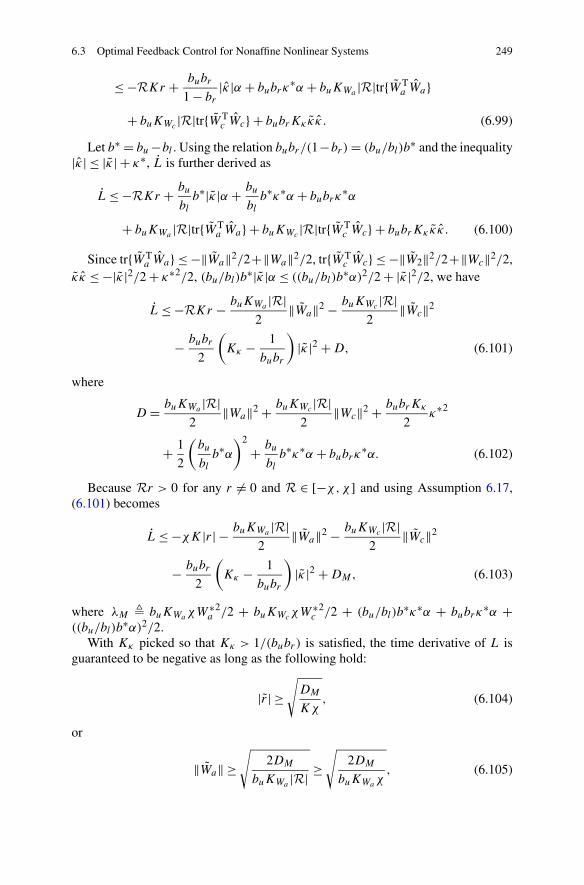
6.3 Optimal Feedback Control for Nonaffine Nonlinear Systems 249
≤ −RKr + bubr
1 − br|κ|α + bubrκ
∗α + buKWa |R|tr{WTa Wa}
+ buKWc |R|tr{WTc Wc} + bubrKκ κκ. (6.99)
Let b∗ = bu−bl . Using the relation bubr/(1−br)= (bu/bl)b∗ and the inequality
|κ| ≤ |κ| + κ∗, L is further derived as
L≤ −RKr + bu
blb∗|κ|α + bu
blb∗κ∗α + bubrκ
∗α
+ buKWa |R|tr{WTa Wa} + buKWc |R|tr{WT
c Wc} + bubrKκ κκ. (6.100)
Since tr{WTa Wa} ≤ −‖Wa‖2/2+‖Wa‖2/2, tr{WT
c Wc} ≤ −‖W2‖2/2+‖Wc‖2/2,κ κ ≤ −|κ|2/2 + κ∗2/2, (bu/bl)b∗|κ|α ≤ ((bu/bl)b
∗α)2/2 + |κ|2/2, we have
L≤ −RKr − buKWa |R|2
‖Wa‖2 − buKWc |R|2
‖Wc‖2
− bubr
2
(Kκ − 1
bubr
)|κ|2 +D, (6.101)
where
D = buKWa |R|2
‖Wa‖2 + buKWc |R|2
‖Wc‖2 + bubrKκ
2κ∗2
+ 1
2
(bu
blb∗α
)2
+ bu
blb∗κ∗α + bubrκ
∗α. (6.102)
Because Rr > 0 for any r �= 0 and R ∈ [−χ,χ] and using Assumption 6.17,(6.101) becomes
L≤ −χK|r| − buKWa |R|2
‖Wa‖2 − buKWc |R|2
‖Wc‖2
− bubr
2
(Kκ − 1
bubr
)|κ|2 +DM, (6.103)
where λM � buKWaχW∗a
2/2 + buKWcχW∗c
2/2 + (bu/bl)b∗κ∗α + bubrκ
∗α +((bu/bl)b
∗α)2/2.With Kκ picked so that Kκ > 1/(bubr) is satisfied, the time derivative of L is
guaranteed to be negative as long as the following hold:
|r| ≥√DM
Kχ, (6.104)
or
‖Wa‖ ≥√
2DM
buKWa |R| ≥√
2DM
buKWaχ, (6.105)
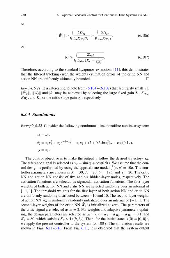
250 6 Optimal Feedback Control for Continuous-Time Systems via ADP
or
‖Wc‖ ≥√
2DM
buKWc |R| ≥√
2DM
buKWcχ, (6.106)
or
|κ| ≥√
2λMbubr(Kκ − 1
bubr). (6.107)
Therefore, according to the standard Lyapunov extensions [11], this demonstratesthat the filtered tracking error, the weights estimation errors of the critic NN andaction NN are uniformly ultimately bounded. �
Remark 6.21 It is interesting to note from (6.104)–(6.107) that arbitrarily small |r|,‖Wa‖, ‖Wc‖ and |κ| may be achieved by selecting the large fixed gain K , KWa ,KWc , and Kκ or the critic slope gain χ , respectively.
6.3.3 Simulations
Example 6.22 Consider the following continuous-time nonaffine nonlinear system:
x1 = x2,
x2 = x1x22 + x2e
−1−x21 − x1x2 + (2 + 0.3sinx2
2)u+ cos(0.1u).
y = x1.
The control objective is to make the output y follow the desired trajectory yd .The reference signal is selected as yd = sin(t)+ cos(0.5t). We assume that the con-trol design is performed by using the approximate model f (x, u) = 10u. The con-troller parameters are chosen as K = 30, Λ= 20, br = 1/3, and χ = 20. The criticNN and action NN consist of five and six hidden-layer nodes, respectively. Theactivation functions are selected as sigmoidal activation functions. The first-layerweights of both action NN and critic NN are selected randomly over an internal of[−1,1]. The threshold weights for the first layer of both action NN and critic NNare uniformly randomly distributed between −10 and 10. The second-layer weightsof action NN Wa is uniformly randomly initialized over an internal of [−1,1]. Thesecond-layer weights of the critic NN Wc is initialized at zero. The parameters ofthe critic signal are selected as m = 2. For weights and adaptive parameters updat-ing, the design parameters are selected as α1 = α2 = α3 = KWa = KWc = 0.1, andKκ = 80, which satisfies Kκ > 1/(bubr). Then, for the initial states x(0)= [0,0]T,we apply the present controller to the system for 100 s. The simulation results areshown in Figs. 6.11–6.16. From Fig. 6.11, it is observed that the system output
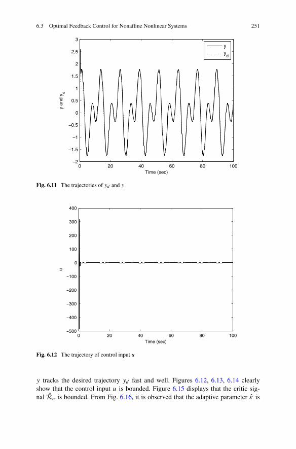
6.3 Optimal Feedback Control for Nonaffine Nonlinear Systems 251
Fig. 6.11 The trajectories of yd and y
Fig. 6.12 The trajectory of control input u
y tracks the desired trajectory yd fast and well. Figures 6.12, 6.13, 6.14 clearlyshow that the control input u is bounded. Figure 6.15 displays that the critic sig-nal Rn is bounded. From Fig. 6.16, it is observed that the adaptive parameter κ is
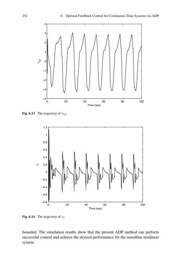
252 6 Optimal Feedback Control for Continuous-Time Systems via ADP
Fig. 6.13 The trajectory of υad
Fig. 6.14 The trajectory of υr
bounded. The simulation results show that the present ADP method can performsuccessful control and achieve the desired performance for the nonaffine nonlinearsystem.
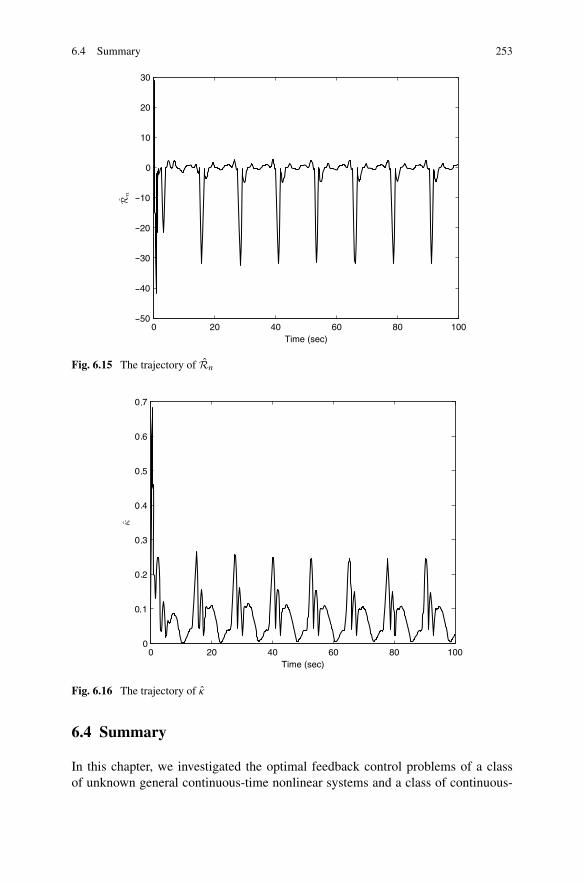
6.4 Summary 253
Fig. 6.15 The trajectory of Rn
Fig. 6.16 The trajectory of κ
6.4 Summary
In this chapter, we investigated the optimal feedback control problems of a classof unknown general continuous-time nonlinear systems and a class of continuous-
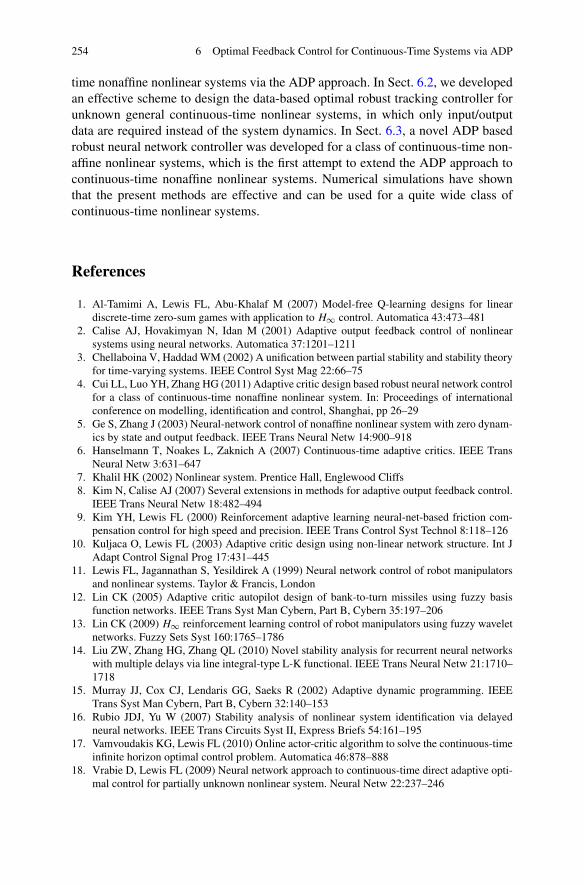
254 6 Optimal Feedback Control for Continuous-Time Systems via ADP
time nonaffine nonlinear systems via the ADP approach. In Sect. 6.2, we developedan effective scheme to design the data-based optimal robust tracking controller forunknown general continuous-time nonlinear systems, in which only input/outputdata are required instead of the system dynamics. In Sect. 6.3, a novel ADP basedrobust neural network controller was developed for a class of continuous-time non-affine nonlinear systems, which is the first attempt to extend the ADP approach tocontinuous-time nonaffine nonlinear systems. Numerical simulations have shownthat the present methods are effective and can be used for a quite wide class ofcontinuous-time nonlinear systems.
References
1. Al-Tamimi A, Lewis FL, Abu-Khalaf M (2007) Model-free Q-learning designs for lineardiscrete-time zero-sum games with application to H∞ control. Automatica 43:473–481
2. Calise AJ, Hovakimyan N, Idan M (2001) Adaptive output feedback control of nonlinearsystems using neural networks. Automatica 37:1201–1211
3. Chellaboina V, Haddad WM (2002) A unification between partial stability and stability theoryfor time-varying systems. IEEE Control Syst Mag 22:66–75
4. Cui LL, Luo YH, Zhang HG (2011) Adaptive critic design based robust neural network controlfor a class of continuous-time nonaffine nonlinear system. In: Proceedings of internationalconference on modelling, identification and control, Shanghai, pp 26–29
5. Ge S, Zhang J (2003) Neural-network control of nonaffine nonlinear system with zero dynam-ics by state and output feedback. IEEE Trans Neural Netw 14:900–918
6. Hanselmann T, Noakes L, Zaknich A (2007) Continuous-time adaptive critics. IEEE TransNeural Netw 3:631–647
7. Khalil HK (2002) Nonlinear system. Prentice Hall, Englewood Cliffs8. Kim N, Calise AJ (2007) Several extensions in methods for adaptive output feedback control.
IEEE Trans Neural Netw 18:482–4949. Kim YH, Lewis FL (2000) Reinforcement adaptive learning neural-net-based friction com-
pensation control for high speed and precision. IEEE Trans Control Syst Technol 8:118–12610. Kuljaca O, Lewis FL (2003) Adaptive critic design using non-linear network structure. Int J
Adapt Control Signal Prog 17:431–44511. Lewis FL, Jagannathan S, Yesildirek A (1999) Neural network control of robot manipulators
and nonlinear systems. Taylor & Francis, London12. Lin CK (2005) Adaptive critic autopilot design of bank-to-turn missiles using fuzzy basis
function networks. IEEE Trans Syst Man Cybern, Part B, Cybern 35:197–20613. Lin CK (2009) H∞ reinforcement learning control of robot manipulators using fuzzy wavelet
networks. Fuzzy Sets Syst 160:1765–178614. Liu ZW, Zhang HG, Zhang QL (2010) Novel stability analysis for recurrent neural networks
with multiple delays via line integral-type L-K functional. IEEE Trans Neural Netw 21:1710–1718
15. Murray JJ, Cox CJ, Lendaris GG, Saeks R (2002) Adaptive dynamic programming. IEEETrans Syst Man Cybern, Part B, Cybern 32:140–153
16. Rubio JDJ, Yu W (2007) Stability analysis of nonlinear system identification via delayedneural networks. IEEE Trans Circuits Syst II, Express Briefs 54:161–195
17. Vamvoudakis KG, Lewis FL (2010) Online actor-critic algorithm to solve the continuous-timeinfinite horizon optimal control problem. Automatica 46:878–888
18. Vrabie D, Lewis FL (2009) Neural network approach to continuous-time direct adaptive opti-mal control for partially unknown nonlinear system. Neural Netw 22:237–246
References 255
19. Vrabie D, Pastravanu O, Abu-Khalaf M, Lewis FL (2009) Adaptive optimal control forcontinuous-time linear systems based on policy iteration. Automatica 45:477–484
20. Wang ZS, Zhang HG, Yu W (2009) Robust stability of Cohen–Grossberg neural networks viastate transmission matrix. IEEE Trans Neural Netw 20:169–174
21. Wang ZS, Zhang HG, Jiang B (2011) LMI-based approach for global asymptotic stabilityanalysis of recurrent neural networks with various delays and structures. IEEE Trans NeuralNetw 22:1032–1045
22. Zhang HG, Wang ZS, Liu DR (2008) Global asymptotic stability of recurrent neural networkswith multiple time-varying delays. IEEE Trans Neural Netw 19:855–873
23. Zhang HG, Li M, Yang J (2009) Fuzzy model-based robust networked control for a class ofnonlinear systems. IEEE Trans Syst Man Cybern, Part A, Syst Hum 39:437–447
24. Zhang HG, Liu ZW, Huang GB (2010) Novel weighting-delay-based stability criteria for re-current neural networks with time-varying delay. IEEE Trans Neural Netw 21:91–106
25. Zhang HG, Cui LL, Zhang X, Luo YH (2011) Data-driven robust approximate optimal track-ing control for unknown general nonlinear systems using adaptive dynamic programmingmethod. IEEE Trans Neural Netw 22(12):2226–2236
26. Zhang HG, Xie XP, Tong SC (2011) Homogeneous polynomially parameter-dependent H∞filter designs of discrete-time fuzzy systems. IEEE Trans Syst Man Cybern, Part B, Cybern41:1313–1322
Chapter 7Several Special Optimal Feedback ControlDesigns Based on ADP
7.1 Introduction
In Chap. 6, we have discussed the optimal feedback control for continuous-timesystems by ADP algorithms. In this chapter, several special optimal feedback controldesigns based on ADP are developed.
In this chapter, we first study the optimal control problem of affine nonlinearswitched systems. Though there are some results on the control of switched systems,most existing results only deal with the state-feedback control problem for switchedsystems, such as [14, 16]. Hence, in order to seek the optimal solution, a noveltwo-stage adaptive dynamic programming (TSADP) is developed. The algorithmcan be divided into two stages: first, for each possible mode, calculate associatedvalue function, and then select the optimal mode for each state. It is shown that thevalue function at each iteration can be characterized pointwise by a set of smoothfunctions recursively generated from TSADP. Moreover, the optimal control policy,continuous control and switching control law included, is explicitly provided in astate-feedback form.
In the second part, the near-optimal control problem of nonlinear descriptor sys-tems is solved by greedy iterative DHP algorithm. A nonquadratic cost functionalis developed in order to deal with the actuator saturation problem. In this way, thegreedy iterative DHP algorithm can be properly introduced to solve the optimalcontrol problem of the original descriptor system.
In the third part, a novel near-optimal control design method for a class of non-linear singularly perturbed systems is developed based on ADP algorithm. By theslow/fast HJB equations and starting from initial performances, the optimal per-formances are converged by neural network approximation and iteration betweencontrol laws and performance indices. It avoids solving the complex HJB equationsdirectly.
In the fourth part, the near-optimal state-feedback control problem is solvedby SNAC method for a class of nonlinear discrete-time systems with control con-straints. Based on the costate function, the greedy iterative DHP algorithm is devel-oped to solve the HJB equation of the system. At each step of the iterative algorithm,
H. Zhang et al., Adaptive Dynamic Programming for Control,Communications and Control Engineering, DOI 10.1007/978-1-4471-4757-2_7,© Springer-Verlag London 2013
257
258 7 Several Special Optimal Feedback Control Designs Based on ADP
a neural network is utilized to approximate the costate function, and then the opti-mal control policy of the system can be computed directly according to the costatefunction, which removes the action network appearing in the ordinary ADP method.
7.2 Optimal Feedback Control for a Class of Switched Systems
7.2.1 Problem Description
Consider the following affine nonlinear discrete-time switched system:
x(t + 1)= fv(t)(x(t))+ gv(t)(x(t))u(t), (7.1)
where x(t) ∈ Rn and u(t) ∈ R
m are the continuous state variable and control in-put, v(t) ∈M is the switching control that determines which subsystem is switchedon to operate. The sequence {〈u(t), v(t)〉}∞0 is called the hybrid control sequencefor system (7.1). Generally, the control is a feedback form, thus we denote thehybrid feedback law as π(x(t)) = 〈μ(x(t)), ν(x(t))〉 : Rn → R
m × M, whereμ(x(t)) : Rn → R
m and ν(x(t)) : Rn → M. Then, the closed-loop system modelwith control policy π is given by
x(t + 1)= fν(x(t))(x(t))+ gν(x(t))(x(t))μ(x(t)). (7.2)
The infinite horizon optimal control problem is to design a hybrid feedback con-trol policy π = 〈μ,ν〉 that minimizes the following cost functional:
Jπ(z)=∞∑
t=0
L(x(t), u(t), v(t)) (7.3)
subject to (7.2), where z ∈ Rn is an arbitrary initial state, i.e., x(0) = z, u(t) =
μ(x(t)) and v(t)= ν(x(t)). L(x,u, v)= xTQvx + uTRvu, Qv > 0 and Rv > 0 arethe cost-to-go weighting matrices for the state and control, respectively.
Definition 7.1 (Admissible Control Policy) The control policy π is admissible if πstabilizes system (7.2) and ∀z, the total cost Jπ(z) is finite, denoted π ∈ΠA.
The following assumption is necessary in the rest of this section.
Assumption 7.2 At least one subsystem is stabilizable.
Assumption 7.2 guarantees the existence of at least one admissible control policy,i.e., the set ΠA is not empty.
Thus, the discrete-time infinite horizon switched optimal control problem can beformulated below.
7.2 Optimal Feedback Control for a Class of Switched Systems 259
Problem 7.3 For a given initial state z ∈ Rn, find the control policy π ∈ ΠA that
minimizes Jπ(z) subject to (7.2).
To solve this problem, define the optimal value function as
J ∗(z)= infπ∈ΠA
Jπ(z), (7.4)
which is characterized by the Bellman equation
J ∗(z)= infu,v
{L(z,u, v)+ J ∗(fv(z)+ gv(z)u)
}. (7.5)
Then, based on traditional dynamic programming theory, the optimal value func-tion can be computed by value iteration, i.e., to start from the initial value functionV0 and update iteratively according to
Vk+1(z)= infu,v
{L(z,u, v)+ Vk(fv(z)+ gv(z)u)} . (7.6)
Unfortunately, the value function for switched systems is in general nonsmooth,even for simple LQR problem (see [15]). Besides, there are two independent vari-ables to minimize the function, thus the iteration with (7.6) is quite complicated andinfeasible.
Notation M = 1, . . . ,M denotes the set of indices of subsystems. The set Lk isdefined as Lk = 1, . . . ,Mk where k is a positive integer or zero. mod (a, b) isan operator that seeks the remainder of a/b and if a is an exact multiple of b, theoperator returns b. The operator [a] takes the largest integer that is no greater than a.N represents the natural number set.
7.2.2 Optimal Feedback Control Based on Two-Stage ADPAlgorithm
In this section, we develop a novel iterative algorithm, termed two-stage adaptivedynamic programming (TSADP), to seek the optimal value function J ∗. The great-est advantage of our algorithm is that it transforms a multivariate optimal controlproblem to be a certain number of univariate optimal control problems at each iter-ation.
To start the iteration, set the initial condition as V0(z) = V(1)0 (z) = 0. For each
i ∈M and l ∈ L0 = {1}, solve
u(l,i)0 (z)= arg min
u
{L(z,u, i)+ V
(l)0 (fi(z)+ gi(z)u)
}(7.7)
and then update the value function using u(l,i)0
V(l)1 (z)= L(z,u
(l,i)0 , i)+ V
(l)0 (fi(z)+ gi(z)u
(l,i)0 ), (7.8)
260 7 Several Special Optimal Feedback Control Designs Based on ADP
where l = (l − 1)×M + i.Let
V1(z)= minl∈L1
{V(l)1 (z)
}, (7.9)
where the set L1 has been defined in Sect. 7.2.1. Therefore, the value function ofthe first iteration is obtained.
Denote
ι0(z)= arg minl∈L1
{V(l)1 (z)
}. (7.10)
Thus, we get the initial control policy π0 = 〈μ0, ν0〉, where
ν0(z)= mod (ι0(z),M) , (7.11)
μ0(z)= u(�ι0(z)/M�+1,ν0(z))
0 (z), (7.12)
and the initial iteration finishes.Suppose Vk is obtained from the (k−1)st iteration, i.e., Vk(z) = minl∈Lk
{V (l)k }.
Then, for each i ∈M and l ∈ Lk , solve
u(l,i)k (z)= arg min
u
{L(z,u, i)+ V
(l)k (fi(z)+ gi(z)u)
}, (7.13)
and update the value function V(l)k+1
V(l)k+1(z)= L(z,u
(l,i)k , i)+ V
(l)k (fi(z)+ gi(z)u
(l,i)k ), (7.14)
where l = (l − 1)×M + i. Then, we get
Vk+1(z)= minl∈Lk+1
{V(l)k+1(z)
}(7.15)
and
ιk(z)= arg minl∈Lk+1
{V(l)k+1(z)
}. (7.16)
Therefore, the control policy at the kth iteration is πk = 〈μk, νk〉, where
νk(z) = mod (ιk(z),M) , (7.17)
μk(z) = u(�ιk(z)/M�+1,νk(z))k (z). (7.18)
The iteration continues according to (7.13)–(7.18).The core part of the two-stage adaptive dynamic programming algorithm is to
solve (7.13) and (7.14) iteratively. Compared with (7.6), there is only one variableu to be determined, which is much easier to be dealt with. As a matter of fact, each
7.2 Optimal Feedback Control for a Class of Switched Systems 261
iteration can be separated into two steps: one to calculate the optimal u(l,i)k and V (l)k+1
with each fixed i and l; then to find the optimal i and l for each z, i.e., to formulateιk(z) and then the control policy πk(z). That is what the term “two-stage” implies.
Remark 7.4 Note that the subscripts of all variables used above, such as Vk , V (·)k and
uk demonstrate the kth iteration of our algorithm. Moreover, the superscript of V (l)k
represents the lth possible component of Vk , while the counterpart of u(l,i)k indicatesthe lth component of Vk−1 as well as the ith subsystem switched on.
Remark 7.5 Apparently, by induction, we conclude that all the functions V (l)k are
smooth because each of them is calculated by conventional value iteration with ini-tial smooth function V0 = 0.
Remark 7.6 Actually, unless the optimal value function is found, the controller lawμk and νk are not used to update the value function Vk+1, then they can be omittedduring the process.
Theorem 7.7 Value function at the kth iteration can be expressed as Vk(z) =minl∈Lk
{V (l)k } and the control policy πk = 〈μk, νk〉 defined in (7.18) and (7.17) is
optimal, i.e.,
〈μk, νk〉 = arg minu,i
{L(z,u, i)+ Vk(fi(z)+ gi(z)u)} . (7.19)
Proof The expression of the value function can be naturally concluded from pre-vious derivation. Besides, according to the principle of dynamic programming, wehave
Vk+1(z) = minu,i
{L(z,u, i)+ Vk(fi(z)+ gi(z)u)}
= minu,i
{L(z,u, i)+ min
l∈Lk
{V(l)k (fi(z)+ gi(z)u)
}}
= minl∈Lk
minu,i
{L(z,u, i)+ V
(l)k (fi(z)+ gi(z)u)
}
= minl∈Lk
mini
{L(z,u
(l,i)k , i)+ V
(l)k (fi(z)+ gi(z)u
(l,i)k )
}. (7.20)
Denote
〈ςk(z), νk(z)〉 = arg minl∈Lk
mini
{L(z,u
(l,i)k , i)+ V
(l)k (fi(z)+ gi(z)u
(l,i)k )
}. (7.21)
Thus, 〈u(ςk(z),νk(z))k (z), νk(z)〉 is the optimal control law for the kth value iteration,i.e., minimizes the first equation in (7.20).
262 7 Several Special Optimal Feedback Control Designs Based on ADP
In addition, note that ιk(z) in (7.16) can be expressed by ςk(z), i.e., ιk =(ςk − 1)×M + νk . As a result, the control policy 〈u(ςk(z),νk(z))k (z), νk(z)〉 is equiv-alent to πk = 〈μk, νk〉 defined in (7.18) and (7.17). Therefore, πk satisfies (7.19). �
Remark 7.8 Different from normal optimal control problem, Vk for switched sys-tem is no longer a single smooth function, it becomes the pointwise minimum of acertain number of value functions obtained from two-stage adaptive dynamic pro-gramming. Similarly, the control policy πk is also state-dependent instead of a singleoptimal feedback control law over the entire state space.
Remark 7.9 Related work has been published in some references, e.g., [11] pro-posed the master-slave procedure (MSP), which was based on some numericalsearch techniques such as MIQP to solve similar optimal control problems. Com-pared with the results in [5, 10–13], our contribution is that the two-stage adap-tive dynamic programming explicitly presents the analytical expression of the opti-mal feedback control policy and its connection to conventional value iteration, cf.(7.17)–(7.19).
In this part, we will prove that the sequence of value functions {Vk} obtained byTSADP is convergent, i.e., there exists a function V∞ satisfying V∞ = limk→∞ Vk ,and derive the relation between V∞ and the optimal value function.
Lemma 7.10 Let {πk = 〈μk, νk〉} be arbitrary sequence of control policy and {Λk}be defined by
Λk+1(z)= L(z, μk, νk)+Λk(fνk (z)+ gνk (z)μk), (7.22)
and {Vk} is obtained by TSADP. If V0(z) = Λ0(z) = 0, thus Vk(z) ≤ Λk(z),∀k ∈ N , z ∈R
n.
Proof According to Theorem 7.7, μk , νk minimize the right-hand side of (7.19)and because V0(z) = Λ0(z) = 0, then by induction it follows that Vk(z) ≤ Λk(z),∀k, z. �
Lemma 7.11 (cf. [4], Boundedness) Under Assumption 7.2, there is a state-dependent upper bound B(z) such that Vk(z)≤ B(z), ∀k ∈N , z ∈ R
n.
Proof Suppose the ith subsystem (fi, gi) is stabilizable (i ∈ M). Denote {V (i)
k } asthe sequence of value functions generated by the iteration only in the i th subsystem
without switching, i.e., V (i)
k+1(z)= minu{L(z,u, i)+ V(i)
k (fi(z)+ gi(z)u)}.Because subsystem i is stabilizable, there must exist an admissible control law
sequence {πk = 〈μk, i〉} where μk can be obtained by
μk = arg minu
{L(z,u, i)+ V
(i)
k (fi(z)+ gi(z)u)}, (7.23)
7.2 Optimal Feedback Control for a Class of Switched Systems 263
and thus V(i)
k (z) < ∞. Therefore, there exists a B(z) such that V (i)
k (z) < B(z).
According to Lemma 7.10, Vk(z) ≤ V(i)
k (z). Consequently, we have Vk(z) ≤V(i)
k (z) < B(z). �
Lemma 7.12 (cf. [4], Monotonicity) The sequence {Vk} generated from TSADP isuniformly monotonically nondecreasing, i.e., Vk(z)≤ Vk+1(z), ∀k ∈ N , z ∈R
n.
Proof Define {Λk} as
Λk+1(z)= L(z,μk+1, νk+1)+Λk(fνk+1(z)+ gνk+1(z)μk+1), (7.24)
moreover,
Vk+1(z)= L(z,μk, νk)+ Vk(fνk (z)+ gνk (z)μk), (7.25)
with Λ0(z)= V0(z)= 0.Next, we are ready to prove that Λk(z)≤ Vk+1(z), ∀z.First, when k = 0, we have
V1(z)−Λ0(z)= L(z,μ0, ν0)≥ 0, (7.26)
i.e., Λ0(z)≤ V1(z), for ∀z.Then, assuming Λk−1(z)≤ Vk(z) holds for ∀z, we obtain
Vk+1(z)−Λk(z)= Vk(z)−Λk−1(z)≥ 0, (7.27)
where z= fνk (z)+ gνk (z)μk . This completes the proof that Λk(z)≤ Vk+1(z).Furthermore, because μk and νk are optimal for Vk , according to Lemma 7.10,
we conclude that Vk(z)≤Λk(z). All in all, it follows that Vk(z)≤ Vk+1(z), ∀k, z. �
Finally, we study its convergence and optimality. Let π = {〈μk, νk〉} be an admis-sible control law sequence and construct the associated sequence {Pk(z)} as follows
Pk+1(z)= L(z, μk, νk)+ Pk(fνk (z)+ gνk (z)μk). (7.28)
By induction, we get
Pk+1(z) = L(x(0), μk, νk)+ Pk(fνk (x(0))+ gνk (x(0))μk)
=1∑
j=0
L(x(j), μk−j , νk−j )+ Pk−1(fνk−1(x(1))+ gνk−1(x(1))μk−1)
...
=k∑
j=0
L(x(j), μk−j , νk−j ), (7.29)
264 7 Several Special Optimal Feedback Control Designs Based on ADP
where x(j + 1)= fνk−j(x(j))+ gνk−j
(x(j))μk−j .As k → ∞, we obtain
P∞(z)= limk→∞
k∑
j=0
L(x(j), μk−j , νk−j ). (7.30)
Define
J ∗(z)= infπP∞(z), (7.31)
then we have the following theorem.
Theorem 7.13 (cf. [4], Convergence and Optimality) Under Assumption 7.2, thesequence {Vk} is convergent and as k → ∞, Vk → J ∗, where J ∗ is the optimalvalue function satisfying
J ∗(z)= infu,v
{L(z,u, v)+ J ∗(fv(z)+ gv(z)u)
}. (7.32)
Proof From Lemmas 7.11 and 7.12, the sequence {Vk} is bounded and monoton-ically nondecreasing, thus we easily conclude that the sequence gets convergentto V∞.
Suppose the control policy is chosen to be π , Lemma 7.10 still holds, i.e., ∀k, z,
Vk(z)≤ Pk(z), (7.33)
then
limk→∞Vk(z)≤ lim
k→∞Pk(z), (7.34)
and
V∞(z)= limk→∞Vk(z)≤ inf
πlimk→∞Pk(z)= J ∗(z). (7.35)
Moreover, from Lemma 7.11, we know that ∀k, Vk is bounded, so is V∞. Thus,by definition of admissible control, the control sequence associated with the V∞must be admissible. Recalling the definition of J ∗ in (7.31), we obtain J ∗ ≤ V∞.Combining it with (7.35), we conclude that J ∗ = V∞, i.e., J ∗ = limk→∞ Vk .
Next, we commence to prove the J ∗ to be optimal.On one hand, according to (7.6), for any k, z, u and v, we have
Vk+1(z)≤ L(z,u, v)+ Vk(fv(z)+ gv(z)u). (7.36)
From Lemma 7.12, the sequence {Vk} is uniformly monotonically nondecreasingand gets convergent to J ∗. Hence, Vk ≤ J ∗ holds for any k, z. Thus, (7.36) becomes
Vk+1(z)≤ L(z,u, v)+ J ∗(fv(z)+ gv(z)u). (7.37)
7.2 Optimal Feedback Control for a Class of Switched Systems 265
As k → ∞, we get
J ∗(z)≤ L(z,u, v)+ J ∗(fv(z)+ gv(z)u). (7.38)
Since u and v are chosen arbitrarily, we have
J ∗(z)≤ infu,v
{L(z,u, v)+ J ∗(fv(z)+ gv(z)u)
}. (7.39)
On the other hand, Vk+1 in (7.6) still satisfies Vk+1 ≤ J ∗. Therefore, (7.6) can bewritten as
J ∗(z)≥ infu,v
{L(z,u, v)+ Vk(fv(z)+ gv(z)u)} . (7.40)
Let k → ∞, we obtain
J ∗(z)≥ infu,v
{L(z,u, v)+ J ∗(fv(z)+ gv(z)u)
}. (7.41)
Combining (7.41) with (7.39), we conclude (7.32), i.e., J ∗ is the optimal valuefunction.
This completes the proof. �
From Theorem 7.13, we conclude that the sequence {Vk} obtained by TSADPconverges to the optimal value function.
It could be seen that the essential part of solving the switched optimal controlproblem is to compute (7.13) and (7.14) iteratively. However, considering the com-plexity and generality of nonlinear systems, there are still large difficulties in solving(7.13) and (7.14) analytically, though it is much easier compared to (7.6). There-fore, for implementation purposes, we apply two kinds of neural network structure,named the critic and action network, respectively, to approximate the value functionand control law at each iteration.
Note that the neural network has a powerful ability to approximate any smoothnonlinear function to arbitrary degree of accuracy, but for discontinuous (or nons-mooth) functions, it is not efficient. Unfortunately, the value function for nonlinearswitched systems at each iterative Vk is the pointwise minimum of all V (l)
k gener-ated from TSADP, which means it is nonsmooth generally. Hence, neural networkcannot be utilized directly to approximate the value function. In this section, a setof neural networks, instead of a single one, is employed to approximate Vk .
According to Remark 7.5, we realize that all V (l)k (z) are smooth. Thus, we can
use the following neural network structures to approximate value function V(l)k (z)
and control law u(l,i)k (z), respectively:
V(l)k (z) =W
(l)k
Tφ(z), (7.42)
u(l,i)k (z) =U
(l,i)k
Tσ(z), (7.43)
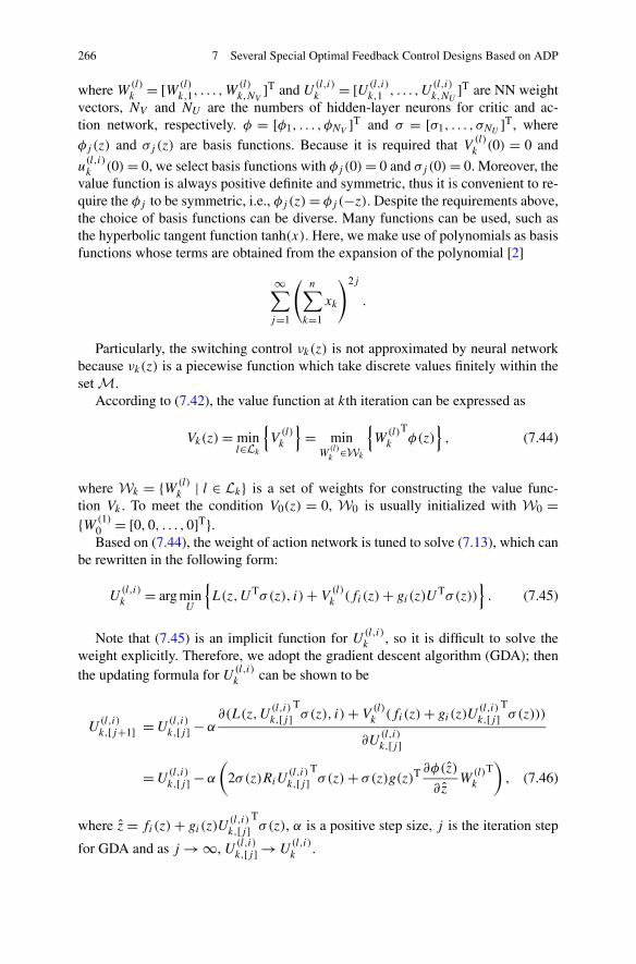
266 7 Several Special Optimal Feedback Control Designs Based on ADP
where W(l)k = [W(l)
k,1, . . . ,W(l)k,NV
]T and U(l,i)k = [U(l,i)
k,1 , . . . ,U(l,i)k,NU
]T are NN weightvectors, NV and NU are the numbers of hidden-layer neurons for critic and ac-tion network, respectively. φ = [φ1, . . . , φNV
]T and σ = [σ1, . . . , σNU]T, where
φj (z) and σj (z) are basis functions. Because it is required that V (l)k (0) = 0 and
u(l,i)k (0)= 0, we select basis functions with φj (0)= 0 and σj (0)= 0. Moreover, the
value function is always positive definite and symmetric, thus it is convenient to re-quire the φj to be symmetric, i.e., φj (z)= φj (−z). Despite the requirements above,the choice of basis functions can be diverse. Many functions can be used, such asthe hyperbolic tangent function tanh(x). Here, we make use of polynomials as basisfunctions whose terms are obtained from the expansion of the polynomial [2]
∞∑
j=1
(n∑
k=1
xk
)2j
.
Particularly, the switching control νk(z) is not approximated by neural networkbecause νk(z) is a piecewise function which take discrete values finitely within theset M.
According to (7.42), the value function at kth iteration can be expressed as
Vk(z)= minl∈Lk
{V(l)k
}= min
W(l)k ∈Wk
{W
(l)k
Tφ(z)
}, (7.44)
where Wk = {W(l)k | l ∈ Lk} is a set of weights for constructing the value func-
tion Vk . To meet the condition V0(z) = 0, W0 is usually initialized with W0 ={W(1)
0 = [0,0, . . . ,0]T}.Based on (7.44), the weight of action network is tuned to solve (7.13), which can
be rewritten in the following form:
U(l,i)k = arg min
U
{L(z,UTσ(z), i)+ V
(l)k (fi(z)+ gi(z)U
Tσ(z))}. (7.45)
Note that (7.45) is an implicit function for U(l,i)k , so it is difficult to solve the
weight explicitly. Therefore, we adopt the gradient descent algorithm (GDA); thenthe updating formula for U(l,i)
k can be shown to be
U(l,i)k,[j+1] =U
(l,i)k,[j ] − α
∂(L(z,U(l,i)k,[j ]
Tσ(z), i)+ V
(l)k (fi(z)+ gi(z)U
(l,i)k,[j ]
Tσ(z)))
∂U(l,i)k,[j ]
=U(l,i)k,[j ] − α
(2σ(z)RiU
(l,i)k,[j ]
Tσ(z)+ σ(z)g(z)T
∂φ(z)
∂zW
(l)k
T), (7.46)
where z = fi(z)+ gi(z)U(l,i)k,[j ]
Tσ(z), α is a positive step size, j is the iteration step
for GDA and as j → ∞, U(l,i)k,[j ] →U
(l,i)k .
7.2 Optimal Feedback Control for a Class of Switched Systems 267
Next, based on U(l,i)k and W
(l)k , we can compute the target cost function for the
critic network according to
d(z,W(l)k ,U
(l,i)k )= L(z,U
(l,i)k
Tσ(z), i)+W
(l)k
Tφ(fi(z)+ gi(z)U
(l,i)k
Tσ(z)).
(7.47)Define the residual error as
e(z)=W(l)k+1
Tφ(z)− d(z,W(l)
k ,U(l,i)k ), (7.48)
where l = (l − 1)×M + i.
The task is to adjust the weight W(l)k+1, such that the error e(z) is minimized on
a training set Ω ∈ Rn. Note that the relation between e(z) and W
(l)k+1 is linear, for
convenient, we employ the method of weighted residuals to realize the iteration. The
weight W(l)k+1 is determined by projecting the residual error onto de(z)/dW(l)
k+1 andsetting the result to zero for any z ∈Ω using the inner product, i.e.,
∫
Ω
∂e(z)
∂W(l)k+1
· eT(z)dz= 0. (7.49)
Substitute e(z) in (7.49) with (7.48), and then we have
∫
Ω
φ(z)
(W
(l)k+1
Tφ(z)− d(z,W(l)
k ,U(l,i)k )
)T
dz= 0. (7.50)
Therefore, a unique solution for W(l)k+1 exists, i.e.,
W(l)k+1 =
(∫
Ω
φ(z)φ(z)Tdz
)−1 ∫
Ω
φ(z)dT(z,W(l)k ,U
(l,i)k )dz. (7.51)
It is worth mentioning that the basis functions we choose, which are linearlyindependent, guarantee that the inverse in (7.51) exists, see [1] for details.
For each i and l, there will be a unique W(l)k+1 generated from (7.51). All the
W(l)k+1 compose a new set Wk+1 = {W(l)
k+1 | l ∈ Lk+1}. Therefore, the value functionat (k + 1)th iteration can be expressed as
Vk+1(z)= minW
(l)k+1∈Wk+1
{W
(l)k+1
Tφ(z)
}. (7.52)
The iteration continues till Vk(z) converges to the optimal value function J ∗(z)or V∞(z). Based on J ∗(z), we obtain the function ι∗(z)
ι∗(z)= arg minl
{V (l)∞ (z)
}, (7.53)
268 7 Several Special Optimal Feedback Control Designs Based on ADP
and the optimal control policy π∗ = 〈μ∗, ν∗〉, where
ν∗(z)= mod(ι∗(z),M
), (7.54)
μ∗(z)= u(�ι∗(z)/M�+1,ν∗(z))∞ (z). (7.55)
Note that at the kth iteration, the number of weights in Wk is Mk , which im-plies that the computation burden grows exponentially as k increases. However, as amatter of fact, not all the weights in Wk make contributes to characterize the valuefunction Vk . The weights that are redundant can be directly removed to simplify thecomputation efficiently. To formalize this idea, firstly we introduce the followingdefinition.
Definition 7.14 (Redundant Weight) A weight W ∈ W is redundant if there existsa W ∈ W \ {W } such that WTφ(z)≤ WTφ(z) holds for all z ∈ R
n.
Obviously, because the redundant weights are never utilized for the value func-tion, there will be no influence on the optimality and convergence of our algorithmif they are ruled out.
By now, we can summarize the TSADP algorithm using neural networks as fol-lows:
1. Initialization. Choose suitable basis functions φ(x) and σ(x). Let W(1)0 =
[0,0, . . . ,0]T, W0 = {W(1)0 }. k = 0.
2. For each l = 1,2, . . . ,Mk , i = 1,2, . . . ,M , update the weight U(l,i)k according
to (7.46) and adjust W(l)k+1 by (7.51) where l = (l − 1)×M + i. All the weights
W(l)k+1 compose the set Wk+1.
3. Rule out redundant weights in Wk+1 based on Definition 7.14.4. If Vk+1 = Vk , go to 5; else k = k + 1 and go to 2.5. Compute the optimal control policy π∗ = 〈μ∗, ν∗〉 by (7.55) and (7.54).
7.2.3 Simulations
In this section, to support the novel theoretical result, we offer a simulation examplefor the present TSADP algorithm.
Consider a general switched optimal control problem with the following twononlinear subsystems.
Subsystem 1:[x1(t + 1)x2(t + 1)
]=[
0.2 sin(x1(t))x2(t)
0.5x2(t)+ 0.5u(t)
]. (7.56)
7.2 Optimal Feedback Control for a Class of Switched Systems 269
Fig. 7.1 Number of remaining weights in Wk
Subsystem 2:[x1(t + 1)x2(t + 1)
]=[
0.5x31(t)x2(t)
0.3x2(t)+ 0.5u(t)
]. (7.57)
The weighting matrices in cost functional are set to be Q1 = Q2 = [ 1 00 1
],
R1 =R2 = 1.To initiate the algorithm, basis functions for critic and action networks are re-
spectively chosen as
φ(x)= [x21 , x1x2, x
22 , x
41 , x
31x2, x
21x
22 , x1x
32 , x
42 , x
61 , x
51x2, x
41x
22 ,
x31x
32 , x
21x
42 , x1x
52 , x
62 ]T,
σ (x)= [x1, x2, x31 , x
21x2, x1x
22 , x
32 , x
51 , x
41x2, x
31x
22 , x
21x
32 , x1x
42 , x
52 ]T,
with initial weight W(1)0 = [0,0, . . . ,0]T. Training set is defined as
Ω = {[x1, x2]T | −2 ≤ x1 ≤ 2,−2 ≤ x2 ≤ 2}.
After 20 steps iteration, the value function gets convergent. At each iteration, thenumber of remaining weights (after redundant weights are deleted) in Wk is shownin Fig. 7.1. At the beginning (when k < 10), the number increases exponentially, buteventually keeps almost constant. There is a slight perturbation, mainly because ofthe approximated errors incurred by neural networks.
Based on the final set W20, we can compute the optimal control law μ∗ and ν∗by (7.55) and (7.54). According to ν∗, we can draw the figure of decision region of
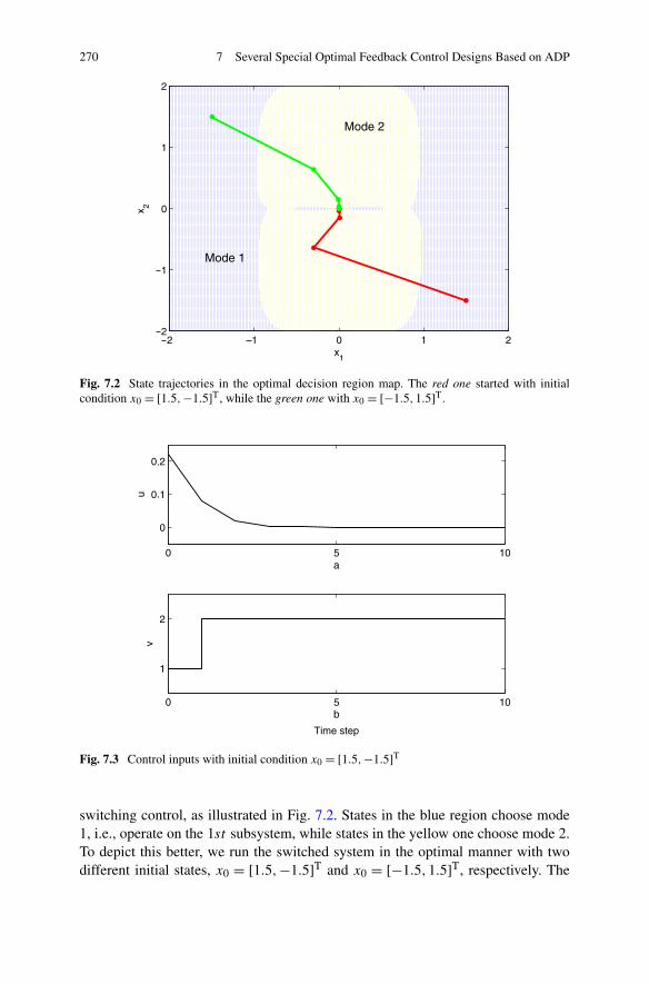
270 7 Several Special Optimal Feedback Control Designs Based on ADP
Fig. 7.2 State trajectories in the optimal decision region map. The red one started with initialcondition x0 = [1.5,−1.5]T, while the green one with x0 = [−1.5,1.5]T.
Fig. 7.3 Control inputs with initial condition x0 = [1.5,−1.5]T
switching control, as illustrated in Fig. 7.2. States in the blue region choose mode1, i.e., operate on the 1st subsystem, while states in the yellow one choose mode 2.To depict this better, we run the switched system in the optimal manner with twodifferent initial states, x0 = [1.5,−1.5]T and x0 = [−1.5,1.5]T, respectively. The
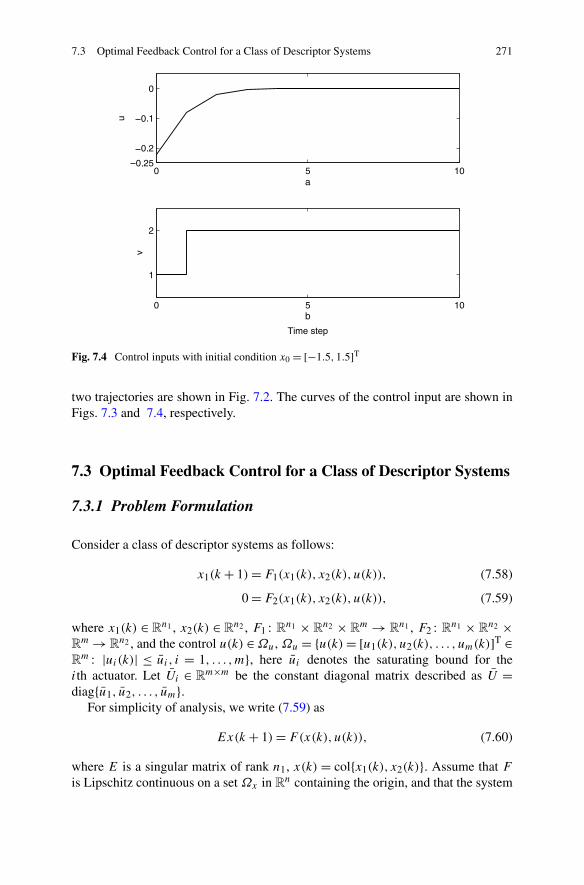
7.3 Optimal Feedback Control for a Class of Descriptor Systems 271
Fig. 7.4 Control inputs with initial condition x0 = [−1.5,1.5]T
two trajectories are shown in Fig. 7.2. The curves of the control input are shown inFigs. 7.3 and 7.4, respectively.
7.3 Optimal Feedback Control for a Class of Descriptor Systems
7.3.1 Problem Formulation
Consider a class of descriptor systems as follows:
x1(k + 1)= F1(x1(k), x2(k), u(k)), (7.58)
0 = F2(x1(k), x2(k), u(k)), (7.59)
where x1(k) ∈ Rn1 , x2(k) ∈ R
n2 , F1 : Rn1 × Rn2 × R
m → Rn1 , F2 : Rn1 × R
n2 ×Rm → R
n2 , and the control u(k) ∈Ωu, Ωu = {u(k)= [u1(k), u2(k), . . . , um(k)]T ∈Rm : |ui(k)| ≤ ui , i = 1, . . . ,m}, here ui denotes the saturating bound for the
ith actuator. Let Ui ∈ Rm×m be the constant diagonal matrix described as U =
diag{u1, u2, . . . , um}.For simplicity of analysis, we write (7.59) as
Ex(k + 1)= F(x(k), u(k)), (7.60)
where E is a singular matrix of rank n1, x(k) = col{x1(k), x2(k)}. Assume that Fis Lipschitz continuous on a set Ωx in R
n containing the origin, and that the system
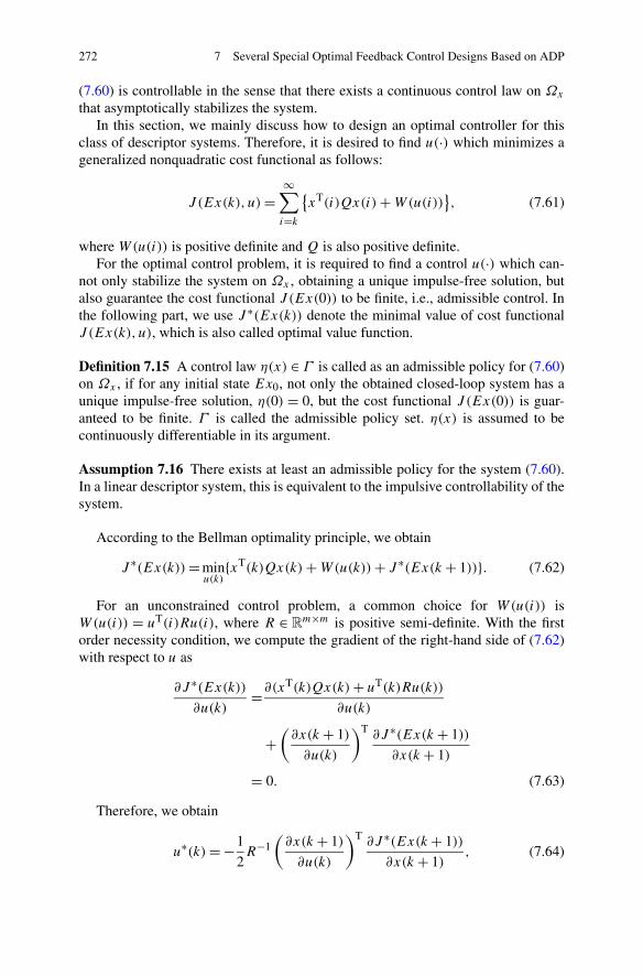
272 7 Several Special Optimal Feedback Control Designs Based on ADP
(7.60) is controllable in the sense that there exists a continuous control law on Ωx
that asymptotically stabilizes the system.In this section, we mainly discuss how to design an optimal controller for this
class of descriptor systems. Therefore, it is desired to find u(·) which minimizes ageneralized nonquadratic cost functional as follows:
J (Ex(k),u)=∞∑
i=k
{xT(i)Qx(i)+W(u(i))
}, (7.61)
where W(u(i)) is positive definite and Q is also positive definite.For the optimal control problem, it is required to find a control u(·) which can-
not only stabilize the system on Ωx , obtaining a unique impulse-free solution, butalso guarantee the cost functional J (Ex(0)) to be finite, i.e., admissible control. Inthe following part, we use J ∗(Ex(k)) denote the minimal value of cost functionalJ (Ex(k),u), which is also called optimal value function.
Definition 7.15 A control law η(x) ∈ Γ is called as an admissible policy for (7.60)on Ωx , if for any initial state Ex0, not only the obtained closed-loop system has aunique impulse-free solution, η(0) = 0, but the cost functional J (Ex(0)) is guar-anteed to be finite. Γ is called the admissible policy set. η(x) is assumed to becontinuously differentiable in its argument.
Assumption 7.16 There exists at least an admissible policy for the system (7.60).In a linear descriptor system, this is equivalent to the impulsive controllability of thesystem.
According to the Bellman optimality principle, we obtain
J ∗(Ex(k))=minu(k)
{xT(k)Qx(k)+W(u(k))+ J ∗(Ex(k + 1))}. (7.62)
For an unconstrained control problem, a common choice for W(u(i)) isW(u(i)) = uT(i)Ru(i), where R ∈ R
m×m is positive semi-definite. With the firstorder necessity condition, we compute the gradient of the right-hand side of (7.62)with respect to u as
∂J ∗(Ex(k))∂u(k)
=∂(xT(k)Qx(k)+ uT(k)Ru(k))
∂u(k)
+(∂x(k + 1)
∂u(k)
)T∂J ∗(Ex(k + 1))
∂x(k + 1)
= 0. (7.63)
Therefore, we obtain
u∗(k)= −1
2R−1
(∂x(k + 1)
∂u(k)
)T∂J ∗(Ex(k + 1))
∂x(k + 1), (7.64)
7.3 Optimal Feedback Control for a Class of Descriptor Systems 273
where J ∗ is the value function corresponding to the optimal control law u∗.However, for constrained control problem, the above derivation is infeasible. To
confront this bounded control problem, we introduce a nonquadratic functional de-rived from the idea by [8] as follows:
W(u(i))= 2∫ u(i)
0ϕ−T(U−1s)URds,
ϕ−1(u(i))= [ψ−1(u1(i)), . . . ,ψ−1(um(i))], (7.65)
where R is positive definite, s ∈ Rm, ϕ ∈ R
m,ψ(·) is a bounded one-to-one func-tion satisfying |ψ(·)| ≤ 1 and belonging to Cp (p ≥ 1) and L2(Ω). Moreover, itis a monotonically increasing odd function with its first derivative bounded by aconstant M . Such a function is easy to find; one example is the hyperbolic tangentfunction ψ(·) = tanh(·). It should be noticed that by the definition above, W(u(i))
is ensured to be positive definite because ψ−1(·) is monotonic odd function and R
is positive definite.Substituting (7.65) into (7.62), we obtain
J ∗(Ex(k))= minu(k)
{xT(k)Qx(k)+ 2
∫ u(k)
0ϕ−T(U−1s)URds
+ J ∗(Ex(k + 1))}. (7.66)
According to the necessary condition of optimal control, the following derivationcan be given:
∂J ∗(Ex(k))∂u(k)
= 2RUϕ−1(U−1u(k))+(∂x(k + 1)
∂u(k)
)T∂J ∗(Ex(k + 1))
∂x(k + 1)= 0.
(7.67)
Therefore, the following formulation can be obtained:
u∗(k)= Uϕ
(−1
2(UR)−1
(∂x(k + 1)
∂u(k)
)T∂J ∗(Ex(k + 1))
∂x(k + 1)
). (7.68)
From (7.68), the optimal control u∗(k) can be directly obtained if the value func-tion J ∗(Ex(k+ 1)) is known. However, there is currently no method for rigorouslysolving for the costate vector of this constrained optimal control problem. There-fore, in the next subsection we will discuss how to utilize an adaptive dynamicprogramming method, named GI-DHP, to solve the near-optimal control solution.
7.3.2 Optimal Controller Design for a Class of Descriptor Systems
In the following, we will give the derivation of the GI-DHP Algorithm.
274 7 Several Special Optimal Feedback Control Designs Based on ADP
Define the costate ETλ(x(k))= ∂V (Ex(k))∂x(k)
. Then, (7.68) can be written as
u∗(k)= Uϕ
(−1
2(UR)−1
(∂Ex(k + 1)
∂u(k)
)T
λ∗(x(k + 1))
). (7.69)
However, there is currently no method for rigorously solving for the costate vec-tor λ∗ of this constrained optimal control problem. Therefore, in the next part, wedevelop an iterative algorithm for computing the costate vector λ∗ and the optimalcontrol u∗.
First, we start with initial value function V [0](Ex(k)) = 0 which is necessaryto the value function. The initial costate vector is set to λ
[0]1 (·) = 0 and then we
compute the optimal control u[0] as follows:
v[0](x(k))= arg minu(k)
{xT(k)Qx(k)+W(v(k))+ V [0](Ex(k + 1))
}. (7.70)
In view of ETλ[i](x(k)) = ∂V [i](Ex(k))∂x(k)
and according to the first order necessitycondition, we obtain
∂(xT(k)Qx(k)+W(u(k))
∂u(k)+(∂Ex(k + 1)
∂u(k)
)T
λ[0](x(k + 1))= 0, (7.71)
i.e.,
v[0](k)= Uϕ
(−1
2(UR)−1
(∂Ex(k + 1)
∂u(k)
)T
λ[0](x(k + 1))
)
= Uϕ
(− 1
2(UR)−1
((∂F1(·)∂u(k)
)T
λ[0]1 (x(k + 1))
+(∂F2(·)∂u(k)
)T
λ[0]2 (x(k + 1))
)), (7.72)
and then update the cost function by
V [1](Ex(k))= xT(k)Qx(k)+W(v[0](k))+ V [0](Ex(k + 1)). (7.73)
For the costate vector, it can be updated by
ETλ[1](x(k))= ∂(xT(k)Qx(k)+W(v[0](k)))∂x(k)
+(∂Ex(k + 1)
∂x(k)
)T
λ[0](x(k + 1)). (7.74)
7.3 Optimal Feedback Control for a Class of Descriptor Systems 275
Let L[0](k) = xT(k)Qx(k) + W(v[0](k)), and then the above equation can beexpanded as
λ[1]1 (x(k))= ∂L[0](k)
∂x1(k)+(
∂F1
∂x1(k)
)T
λ[0]1 (x(k + 1))
+(
∂F2
∂x1(k)
)T
λ[0]2 (x(k + 1)) (7.75)
and
0 = ∂L[0](k)∂x2(k)
+(
∂F1
∂x2(k)
)T
λ[0]1 (x(k + 1))+
(∂F2
∂x2(k)
)T
λ[0]2 (x(k + 1)). (7.76)
Therefore, for the ith iteration, we have
v[i](x(k))= arg minu(k)
{xT(k)Qx(k)+W(u(k))+ V [i](Ex(k + 1))
}. (7.77)
Also, according to the first order necessity condition, we obtain
∂(xT(k)Qx(k)+W(u(k))
∂u(k)+(∂x(k + 1)
∂u(k)
)T∂V [i](Ex(k + 1))
∂x(k + 1)= 0, (7.78)
i.e.,
v[i](k)= Uϕ
[−1
2(UR)−1
(∂Ex(k + 1)
∂u(k)
)T
λ[i](x(k + 1))
]
= Uϕ
[− 1
2(UR)−1
((∂F1(·)∂u(k)
)T
λ[i]1 (x(k + 1))
+(∂F2(·)∂u(k)
)T
λ[i]2 (x(k + 1))
)]. (7.79)
The updated value function is given as
V [i+1](Ex(k))= xT(k)Qx(k)+W(v[i](k))+ V [i](Ex(k + 1)). (7.80)
In view of ETλ[i+1](x(k))= ∂V [i+1](Ex(k))∂x(k)
, we have
∂V [i+1](Ex(k))∂x(k)
= ∂(xT(k)Qx(k)+W(v[i](k)))∂x(k)
276 7 Several Special Optimal Feedback Control Designs Based on ADP
+(∂v[i](x(k))∂x(k)
)T∂(xT(k)Qx(k)+W(v[i](k)))
∂v[i](x(k))
+(∂x(k + 1)
∂x(k)
)T∂V [i](Ex(k + 1))
∂x(k + 1)
+(∂v[i](x(k))∂x(k)
)T(∂x(k + 1)
∂v[i](x(k))
)T∂V [i](Ex(k + 1))
∂x(k + 1)
= ∂(x(k)TQx(k)+W(v[i](k)))∂x(k)
+(∂Ex(k+1)
∂x(k)
)T
λ[i](x(k+1)).
(7.81)
Combining with (7.78), (7.81) can be changed into
ETλ[i+1](x(k))= ∂(xT(k)Qx(k)+W(v[i](k)))∂x(k)
+(∂Ex(k + 1)
∂x(k)
)T
λ[i](x(k + 1)). (7.82)
Similarly, the above equation can be expanded into
λ[i+1]1 (x(k))= ∂L[i](k)
∂x1(k)+(
∂F1
∂x1(k)
)T
λ[i]1 (x(k + 1))
+(
∂F2
∂x1(k)
)T
λ[i]2(x(k + 1)) (7.83)
and
0 = ∂L[i](k)∂x2(k)
+(
∂F1
∂x2(k)
)T
λ[i]1 (x(k + 1))+
(∂F2
∂x2(k)
)T
λ[i]2 (x(k + 1)). (7.84)
Therefore, the GI-DHP iterative scheme iterates between
v[i](k)= Uϕ
[− 1
2(UR)−1
((∂F1(·)∂u(k)
)T
λ[i]1 (x(k + 1))
+(∂F2(·)∂u(k)
)T
λ[i]2 (x(k + 1))
)], (7.85)
λ[i+1]1 (x(k))= ∂L[i](k)
∂x1(k)+(
∂F1
∂x1(k)
)λ
[i]1 (x(k + 1))
+(
∂F2
∂x1(k)
)λ
[i]2 (x(k + 1)), (7.86)
7.3 Optimal Feedback Control for a Class of Descriptor Systems 277
and
0 = ∂L[i](k)∂x2(k)
+(
∂F1
∂x2(k)
)λ
[i]1 (x(k + 1))+
(∂F2
∂x2(k)
)λ
[i]2 (x(k + 1)). (7.87)
At each iteration step, the λ[i]1 (·) is computed iteratively by (7.86) while the λ[i]
2 (·)is computed by the constraint equation (7.87). With known λ
[i]1 (·) and λ
[i]2 (·), the
control vi(·) can be obtained by (7.85).In the following part, we will prove that by the above iterative process, the opti-
mal control u∗ and the costate λ∗ can be obtained with V [i] → J ∗, λ[i] → λ∗ andthe control policy v[i] → u∗ as i → ∞.
For convenience of analysis, we first present a lemma as follows.
Lemma 7.17 Let μ[i] be arbitrary sequence of control policies, and v[i] is the poli-cies in (7.77). Let V [i] be (7.80) and Λ[i] as
Λ[i+1](Ex(k))= xT(k)Qx(k)+W(μ[i](k))+Λ[i](Ex(k + 1)), (7.88)
If V [0] =Λ[0] = 0, then V [i] ≤Λ[i], ∀i .
Lemma 7.18 Let the sequence{V [i]} be defined as (7.80). If the system is control-
lable, then there is an upper bound Y such that 0 ≤ V [i] ≤ Y ∀i .
Proof Let η(x(k)) be any stabilizing and admissible control input, and let V [0] =Z[0] = 0 where V [i] is updated as (7.80) and Z[i] is updated as
Z[i+1](Ex(k))= xT(k)Qx(k)+W(η(k))+Z[i](Ex([k + 1])). (7.89)
It follows that the difference
Z[i+1](Ex(k))−Z[i](Ex(k))= Z[i](Ex(k + 1))−Z[i−1](Ex(k + 1))
= Z[i−1](Ex(k + 2))−Z[i−2](Ex(k + 2))
= Z[i−2](Ex(k + 3))−Z[i−3](Ex(k + 3))
...
= Z[1](Ex(k + i))−Z[0](Ex(k + i)). (7.90)
Then, the following relation can be obtained:
Z[i+1](Ex(k))−Z[i](Ex(k))= Z[1](Ex(k + i))−Z[0](Ex(k + i)). (7.91)
Since Z[0](Ex(·))= 0, we have
Z[i+1](Ex(k))= Z[1](Ex(k + i))+Z[i](Ex(k))
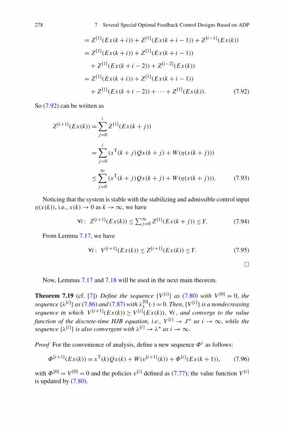
278 7 Several Special Optimal Feedback Control Designs Based on ADP
= Z[1](Ex(k + i))+Z[1](Ex(k + i − 1))+Z[i−1](Ex(k))
= Z[1](Ex(k + i))+Z[1](Ex(k + i − 1))
+Z[1](Ex(k + i − 2))+Z[i−2](Ex(k))
= Z[1](Ex(k + i))+Z[1](Ex(k + i − 1))
+Z[1](Ex(k + i − 2))+ · · · +Z[1](Ex(k)). (7.92)
So (7.92) can be written as
Z[i+1](Ex(k))=i∑
j=0
Z[1](Ex(k + j))
=i∑
j=0
(xT(k + j)Qx(k + j)+W(η(x(k + j)))
≤∞∑
j=0
(xT(k + j)Qx(k + j)+W(η(x(k + j))). (7.93)
Noticing that the system is stable with the stabilizing and admissible control inputη(x(k)), i.e., x(k)→ 0 as k → ∞, we have
∀i : Z[i+1](Ex(k))≤∑∞j=0 Z
[1](Ex(k + j))≤Y. (7.94)
From Lemma 7.17, we have
∀i : V [i+1](Ex(k))≤Z[i+1](Ex(k))≤Y. (7.95)
�
Now, Lemmas 7.17 and 7.18 will be used in the next main theorem.
Theorem 7.19 (cf. [7]) Define the sequence {V [i]} as (7.80) with V [0] = 0, thesequence {λ[i]} as (7.86) and (7.87) with λ[0]
1 (·)= 0. Then, {V [i]} is a nondecreasingsequence in which V [i+1](Ex(k))≥ V [i](Ex(k)), ∀i , and converge to the valuefunction of the discrete-time HJB equation, i.e., V [i] → J ∗ as i → ∞, while thesequence {λ[i]} is also convergent with λ[i] → λ∗ as i → ∞.
Proof For the convenience of analysis, define a new sequence Φi as follows:
Φ[i+1](Ex(k))= xT(k)Qx(k)+W(v[i+1](k))+Φ[i](Ex(k + 1)), (7.96)
with Φ[0] = V [0] = 0 and the policies v[i] defined as (7.77); the value function V [i]is updated by (7.80).
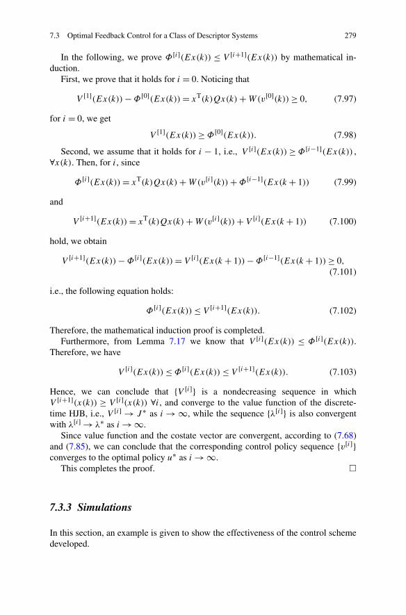
7.3 Optimal Feedback Control for a Class of Descriptor Systems 279
In the following, we prove Φ[i](Ex(k)) ≤ V [i+1](Ex(k)) by mathematical in-duction.
First, we prove that it holds for i = 0. Noticing that
V [1](Ex(k))−Φ[0](Ex(k))= xT(k)Qx(k)+W(v[0](k))≥ 0, (7.97)
for i = 0, we get
V [1](Ex(k))≥Φ[0](Ex(k)). (7.98)
Second, we assume that it holds for i − 1, i.e., V [i](Ex(k))≥Φ[i−1](Ex(k)) ,∀x(k). Then, for i, since
Φ[i](Ex(k))= xT(k)Qx(k)+W(v[i](k))+Φ[i−1](Ex(k + 1)) (7.99)
and
V [i+1](Ex(k))= xT(k)Qx(k)+W(v[i](k))+ V [i](Ex(k + 1)) (7.100)
hold, we obtain
V [i+1](Ex(k))−Φ[i](Ex(k))= V [i](Ex(k + 1))−Φ[i−1](Ex(k + 1))≥ 0,(7.101)
i.e., the following equation holds:
Φ[i](Ex(k))≤ V [i+1](Ex(k)). (7.102)
Therefore, the mathematical induction proof is completed.Furthermore, from Lemma 7.17 we know that V [i](Ex(k)) ≤ Φ[i](Ex(k)).
Therefore, we have
V [i](Ex(k))≤Φ[i](Ex(k))≤ V [i+1](Ex(k)). (7.103)
Hence, we can conclude that {V [i]} is a nondecreasing sequence in whichV [i+1](x(k)) ≥ V [i](x(k)) ∀i, and converge to the value function of the discrete-time HJB, i.e., V [i] → J ∗ as i → ∞, while the sequence {λ[i]} is also convergentwith λ[i] → λ∗ as i → ∞.
Since value function and the costate vector are convergent, according to (7.68)and (7.85), we can conclude that the corresponding control policy sequence {v[i]}converges to the optimal policy u∗ as i → ∞.
This completes the proof. �
7.3.3 Simulations
In this section, an example is given to show the effectiveness of the control schemedeveloped.
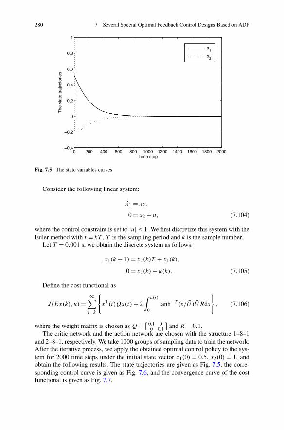
280 7 Several Special Optimal Feedback Control Designs Based on ADP
Fig. 7.5 The state variables curves
Consider the following linear system:
x1 = x2,
0 = x2 + u, (7.104)
where the control constraint is set to |u| ≤ 1. We first discretize this system with theEuler method with t = kT , T is the sampling period and k is the sample number.
Let T = 0.001 s, we obtain the discrete system as follows:
x1(k + 1)= x2(k)T + x1(k),
0 = x2(k)+ u(k). (7.105)
Define the cost functional as
J (Ex(k),u)=∞∑
i=k
{xT(i)Qx(i)+ 2
∫ u(i)
0tanh−T (s/U)URds
}, (7.106)
where the weight matrix is chosen as Q= [ 0.1 00 0.1
]and R = 0.1.
The critic network and the action network are chosen with the structure 1–8–1and 2–8–1, respectively. We take 1000 groups of sampling data to train the network.After the iterative process, we apply the obtained optimal control policy to the sys-tem for 2000 time steps under the initial state vector x1(0) = 0.5, x2(0) = 1, andobtain the following results. The state trajectories are given as Fig. 7.5, the corre-sponding control curve is given as Fig. 7.6, and the convergence curve of the costfunctional is given as Fig. 7.7.
7.4 Optimal Feedback Control for a Class of Singularly Perturbed Systems 281
Fig. 7.6 The control curve
Fig. 7.7 The convergence curve of costate vector
7.4 Optimal Feedback Control for a Class of SingularlyPerturbed Systems
7.4.1 Problem Formulation
Consider the following nonlinear singularly perturbed systems:
x1 = f11(x1)+ f12(x1)x2 + g1(x1)u, (7.107)
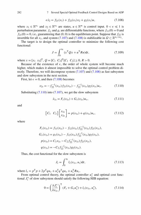
282 7 Several Special Optimal Feedback Control Designs Based on ADP
εx2 = f21(x1)+ f22(x1)x2 + g2(x1)u, (7.108)
where x1 ∈ Rn1 and x2 ∈ R
n2 are states, u ∈ Rm is control input. 0 < ε � 1 is
perturbation parameter. fij and gi are differentiable functions, where f11(0)= 0 andf21(0)= 0, i.e., guaranteeing that (0,0) is the equilibrium point. Suppose that f22 isinvertible for all x1, and system (7.107) and (7.108) is stabilizable in Ω ⊂ R
n1+n2 .The target is to design the optimal controller to minimize the following cost
functional:
J =∫ ∞
0(xTQx + uTRu)dt , (7.109)
where x = [x1 x2]T, Q= [C1 C2]T[C1 C2] ≥ 0, R > 0.Because of the existence of ε, the order of whole system will become much
higher, which makes it almost impossible to solve the optimal control problem di-rectly. Therefore, we will decompose system (7.107) and (7.108) as fast subsystemand slow subsystem in the next section.
First, let ε = 0, and then (7.108) becomes
x2s = −f−122 (x1s)f21(x1s)− f−1
22 (x1s)g2(x1s)us. (7.110)
Substituting (7.110) into (7.107), we get the slow subsystem
x1s = Fs(x1s)+Gs(x1s)us, (7.111)
and
[C1 C2
][x1sx2s
]= p(x1s)+ q(x1s)us, (7.112)
where
Fs(x1s)= f11(x1s)− f12(x1s)f−122 (x1s)f21(x1s),
Gs(x1s)= g1(x1s)− f12(x1s)f−122 (x1s)g2(x1s),
p(x1s)= C1x1s −C2f−122 (x1s)f21(x1s),
q(x1s)= −C2f−122 (x1s)g2(x1s).
Thus, the cost functional for the slow subsystem is
Js =∫ ∞
0ls(x1s , us)dt, (7.113)
where ls = pTp + 2pTqus + uTs q
Tqus + uTs Rus .
From optimal control theory, the optimal controller u∗s and optimal cost func-
tional J ∗s of slow subsystem should satisfy the following HJB equation:
0 =(∂J ∗
s
∂x1s
)T
(Fs +Gsu∗s )+ ls(x1s , u
∗s ), (7.114)
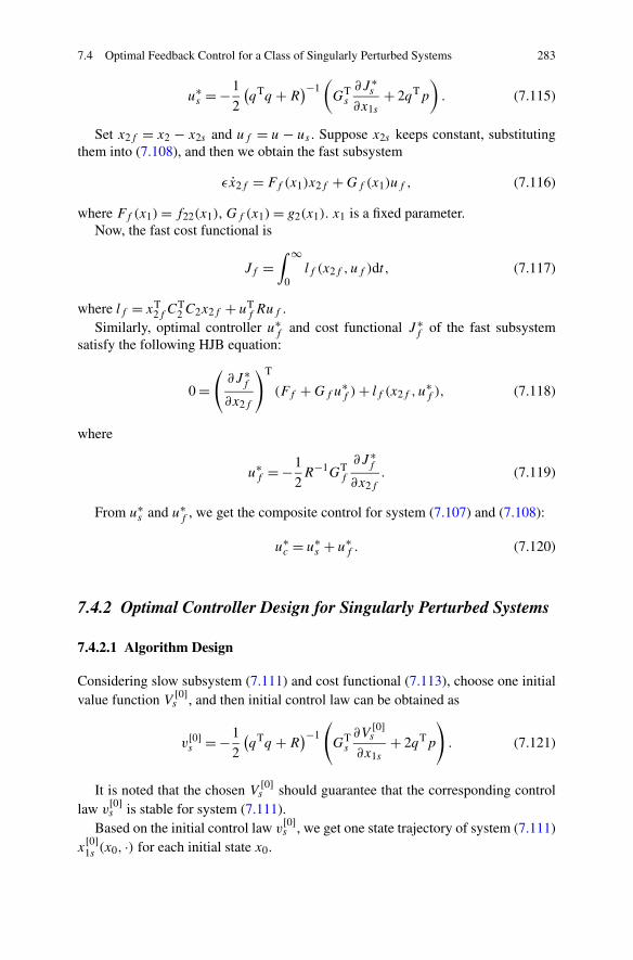
7.4 Optimal Feedback Control for a Class of Singularly Perturbed Systems 283
u∗s = −1
2
(qTq +R
)−1(GTs
∂J ∗s
∂x1s+ 2qTp
). (7.115)
Set x2f = x2 − x2s and uf = u − us . Suppose x2s keeps constant, substitutingthem into (7.108), and then we obtain the fast subsystem
εx2f = Ff (x1)x2f +Gf (x1)uf , (7.116)
where Ff (x1)= f22(x1), Gf (x1)= g2(x1). x1 is a fixed parameter.Now, the fast cost functional is
Jf =∫ ∞
0lf (x2f , uf )dt, (7.117)
where lf = xT2f C
T2 C2x2f + uT
f Ruf .Similarly, optimal controller u∗
f and cost functional J ∗f of the fast subsystem
satisfy the following HJB equation:
0 =(∂J ∗
f
∂x2f
)T
(Ff +Gf u∗f )+ lf (x2f , u
∗f ), (7.118)
where
u∗f = −1
2R−1GT
f
∂J ∗f
∂x2f. (7.119)
From u∗s and u∗
f , we get the composite control for system (7.107) and (7.108):
u∗c = u∗
s + u∗f . (7.120)
7.4.2 Optimal Controller Design for Singularly Perturbed Systems
7.4.2.1 Algorithm Design
Considering slow subsystem (7.111) and cost functional (7.113), choose one initialvalue function V
[0]s , and then initial control law can be obtained as
v[0]s = −1
2
(qTq +R
)−1
(GTs
∂V[0]s
∂x1s+ 2qTp
). (7.121)
It is noted that the chosen V[0]s should guarantee that the corresponding control
law v[0]s is stable for system (7.111).
Based on the initial control law v[0]s , we get one state trajectory of system (7.111)
x[0]1s (x0, ·) for each initial state x0.
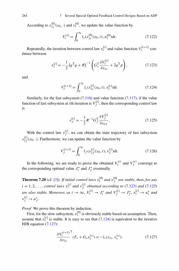
284 7 Several Special Optimal Feedback Control Designs Based on ADP
According to x[0]1s (x0, ·) and v
[0]s , we update the value function by
V [1]s =
∫ ∞
0ls(x
[0]1s (x0, t), u
[0]s )dt . (7.122)
Repeatedly, the iteration between control law v[i]s and value function V [i+1]
s con-tinues between
v[i]s = −1
2
(qTq +R
)−1
(GTs
∂V[i]s
∂x1s+ 2qTp
), (7.123)
and
V [i+1]s =
∫ ∞
0ls(x
[i]1s (x0, t), v
[i]s )dt . (7.124)
Similarly, for the fast subsystem (7.116) and value function (7.117), if the valuefunction of fast subsystem at ith iteration is V [i]
f , then the corresponding control lawis
v[i]f = −1
2R−1GT
f
∂V[i]f
∂x2f. (7.125)
With the control law v[i]f , we can obtain the state trajectory of fast subsystem
x[i]2f (x0, ·). Furthermore, we can update the value function by
V[i+1]f =
∫ ∞
0lf (x
[i]2f (x0, t), v
[i]f )dt . (7.126)
In the following, we are ready to prove the obtained V(i)s and V
(i)f converge to
the corresponding optimal value J ∗s and J ∗
f eventually.
Theorem 7.20 (cf. [3]) If initial control laws v[0]s and v
[0]f are stable, then, for any
i = 1,2, . . . , control laws v[i]s and v
[i]f obtained according to (7.123) and (7.125)
are also stable. Moreover, as i → ∞, V [i]s → J ∗
s and V[i]f → J ∗
f , v[i]s → u∗
s and
v[i]f → u∗
f .
Proof We prove this theorem by induction.First, for the slow subsystem, v[0]
s is obviously stable based on assumption. Then,assume that v[i]
s is stable. It is easy to see that (7.124) is equivalent to the iterativeHJB equation (7.127):
∂V(i+1)s
∂x1s
T
(Fs +Gsv(i)s )= −ls(x1s , v
(i)s ). (7.127)
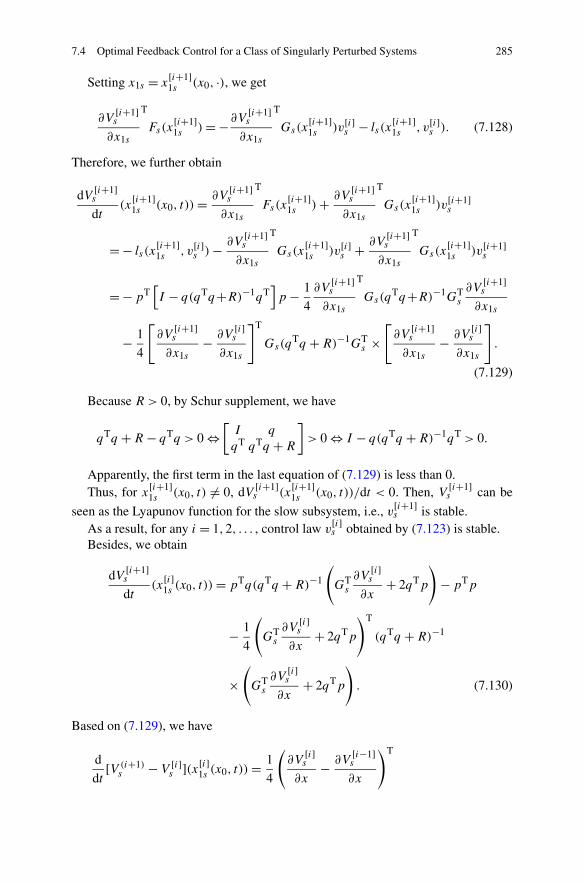
7.4 Optimal Feedback Control for a Class of Singularly Perturbed Systems 285
Setting x1s = x[i+1]1s (x0, ·), we get
∂V[i+1]s
∂x1s
T
Fs(x[i+1]1s )= −∂V
[i+1]s
∂x1s
T
Gs(x[i+1]1s )v[i]
s − ls(x[i+1]1s , v[i]
s ). (7.128)
Therefore, we further obtain
dV [i+1]s
dt(x
[i+1]1s (x0, t))= ∂V
[i+1]s
∂x1s
T
Fs(x[i+1]1s )+ ∂V
[i+1]s
∂x1s
T
Gs(x[i+1]1s )v[i+1]
s
= − ls(x[i+1]1s , v[i]
s )− ∂V[i+1]s
∂x1s
T
Gs(x[i+1]1s )v[i]
s + ∂V[i+1]s
∂x1s
T
Gs(x[i+1]1s )v[i+1]
s
= − pT[I − q(qTq+R)−1qT
]p − 1
4
∂V[i+1]s
∂x1s
T
Gs(qTq+R)−1GT
s
∂V[i+1]s
∂x1s
− 1
4
[∂V
[i+1]s
∂x1s− ∂V
[i]s
∂x1s
]T
Gs(qTq +R)−1GT
s ×[∂V
[i+1]s
∂x1s− ∂V
[i]s
∂x1s
].
(7.129)
Because R > 0, by Schur supplement, we have
qTq +R − qTq > 0 ⇔[I q
qT qTq +R
]> 0 ⇔ I − q(qTq +R)−1qT > 0.
Apparently, the first term in the last equation of (7.129) is less than 0.Thus, for x[i+1]
1s (x0, t) �= 0, dV [i+1]s (x
[i+1]1s (x0, t))/dt < 0. Then, V [i+1]
s can be
seen as the Lyapunov function for the slow subsystem, i.e., v[i+1]s is stable.
As a result, for any i = 1,2, . . . , control law v[i]s obtained by (7.123) is stable.
Besides, we obtain
dV [i+1]s
dt(x
[i]1s (x0, t))= pTq(qTq +R)−1
(GTs
∂V[i]s
∂x+ 2qTp
)− pTp
− 1
4
(GTs
∂V[i]s
∂x+ 2qTp
)T
(qTq +R)−1
×(GTs
∂V[i]s
∂x+ 2qTp
). (7.130)
Based on (7.129), we have
d
dt[V (i+1)
s − V [i]s ](x[i]
1s (x0, t))= 1
4
(∂V
[i]s
∂x− ∂V
[i−1]s
∂x
)T
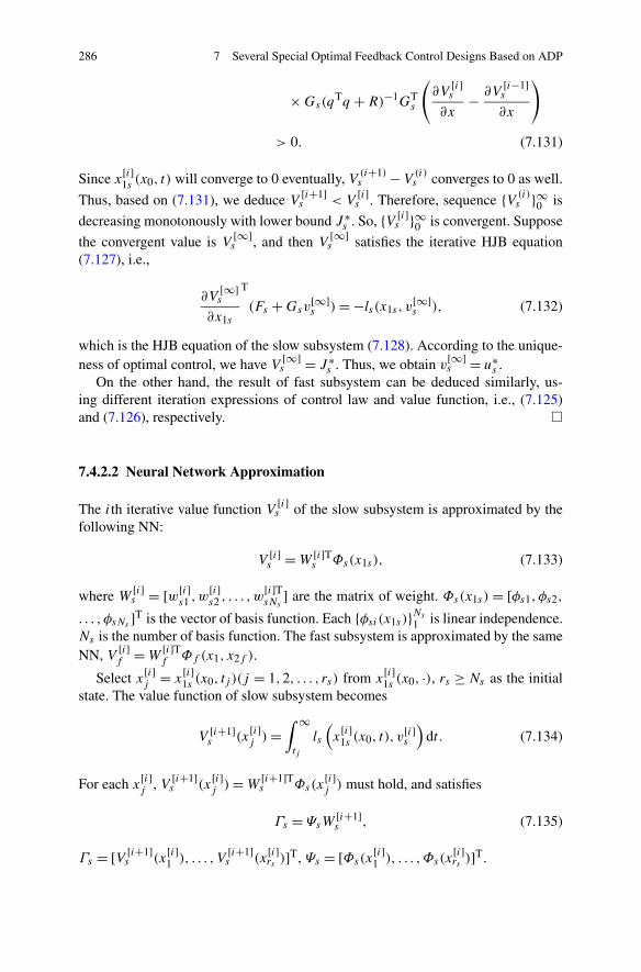
286 7 Several Special Optimal Feedback Control Designs Based on ADP
×Gs(qTq +R)−1GT
s
(∂V
[i]s
∂x− ∂V
[i−1]s
∂x
)
> 0. (7.131)
Since x[i]1s (x0, t) will converge to 0 eventually, V (i+1)
s −V(i)s converges to 0 as well.
Thus, based on (7.131), we deduce V[i+1]s < V
[i]s . Therefore, sequence {V (i)
s }∞0 is
decreasing monotonously with lower bound J ∗s . So, {V [i]
s }∞0 is convergent. Suppose
the convergent value is V[∞]s , and then V
[∞]s satisfies the iterative HJB equation
(7.127), i.e.,
∂V[∞]s
∂x1s
T
(Fs +Gsv[∞]s )= −ls(x1s , v
[∞]s ), (7.132)
which is the HJB equation of the slow subsystem (7.128). According to the unique-ness of optimal control, we have V [∞]
s = J ∗s . Thus, we obtain v
[∞]s = u∗
s .On the other hand, the result of fast subsystem can be deduced similarly, us-
ing different iteration expressions of control law and value function, i.e., (7.125)and (7.126), respectively. �
7.4.2.2 Neural Network Approximation
The ith iterative value function V[i]s of the slow subsystem is approximated by the
following NN:
V [i]s =W [i]T
s Φs(x1s), (7.133)
where W [i]s = [w[i]
s1 ,w[i]s2 , . . . ,w
[i]TsNs
] are the matrix of weight. Φs(x1s) = [φs1, φs2,. . . , φsNs ]T is the vector of basis function. Each {φsi(x1s)}Ns
1 is linear independence.Ns is the number of basis function. The fast subsystem is approximated by the sameNN, V [i]
f =W[i]Tf Φf (x1, x2f ).
Select x[i]j = x
[i]1s (x0, tj )(j = 1,2, . . . , rs) from x
[i]1s (x0, ·), rs ≥ Ns as the initial
state. The value function of slow subsystem becomes
V [i+1]s (x
[i]j )=
∫ ∞
tj
ls
(x
[i]1s (x0, t), v
[i]s
)dt . (7.134)
For each x[i]j , V [i+1]
s (x[i]j )=W
[i+1]Ts Φs(x
[i]j ) must hold, and satisfies
Γs = ΨsW[i+1]s , (7.135)
Γs = [V [i+1]s (x
[i]1 ), . . . , V
[i+1]s (x
[i]rs )]T, Ψs = [Φs(x
[i]1 ), . . . ,Φs(x
[i]rs )]T.
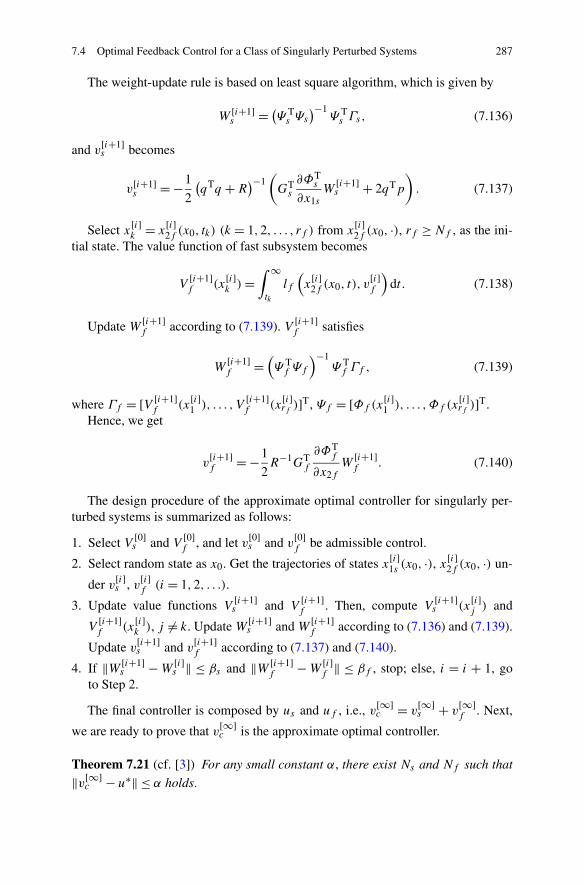
7.4 Optimal Feedback Control for a Class of Singularly Perturbed Systems 287
The weight-update rule is based on least square algorithm, which is given by
W [i+1]s = (
Ψ Ts Ψs
)−1Ψ Ts Γs, (7.136)
and v[i+1]s becomes
v[i+1]s = −1
2
(qTq +R
)−1(GTs
∂ΦTs
∂x1sW
[i+1]s + 2qTp
). (7.137)
Select x[i]k = x
[i]2f (x0, tk) (k = 1,2, . . . , rf ) from x
[i]2f (x0, ·), rf ≥ Nf , as the ini-
tial state. The value function of fast subsystem becomes
V[i+1]f (x
[i]k )=
∫ ∞
tk
lf
(x
[i]2f (x0, t), v
[i]f
)dt . (7.138)
Update W [i+1]f according to (7.139). V [i+1]
f satisfies
W[i+1]f =
(Ψ Tf Ψf
)−1Ψ Tf Γf , (7.139)
where Γf = [V [i+1]f (x
[i]1 ), . . . , V
[i+1]f (x
[i]rf )]T, Ψf = [Φf (x
[i]1 ), . . . ,Φf (x
[i]rf )]T.
Hence, we get
v[i+1]f = −1
2R−1GT
f
∂ΦTf
∂x2fW
[i+1]f . (7.140)
The design procedure of the approximate optimal controller for singularly per-turbed systems is summarized as follows:
1. Select V [0]s and V
[0]f , and let v[0]
s and v[0]f be admissible control.
2. Select random state as x0. Get the trajectories of states x[i]1s (x0, ·), x[i]
2f (x0, ·) un-
der v[i]s , v[i]
f (i = 1,2, . . .).
3. Update value functions V[i+1]s and V
[i+1]f . Then, compute V
[i+1]s (x
[i]j ) and
V[i+1]f (x
[i]k ), j �= k. Update W [i+1]
s and W [i+1]f according to (7.136) and (7.139).
Update v[i+1]s and v
[i+1]f according to (7.137) and (7.140).
4. If ‖W [i+1]s −W
[i]s ‖ ≤ βs and ‖W [i+1]
f −W[i]f ‖ ≤ βf , stop; else, i = i + 1, go
to Step 2.
The final controller is composed by us and uf , i.e., v[∞]c = v
[∞]s + v
[∞]f . Next,
we are ready to prove that v[∞]c is the approximate optimal controller.
Theorem 7.21 (cf. [3]) For any small constant α, there exist Ns and Nf such that
‖v[∞]c − u∗‖ ≤ α holds.
288 7 Several Special Optimal Feedback Control Designs Based on ADP
Proof From Theorem 7.20, we know that we always get v[i]s → u∗
s and v[i]f → u∗
fwhen i → ∞ if Ns and Nf are chosen appropriately.
It means that for ∀αs and ∀αf , there exists i such that ‖v[i]s − u∗
s‖ ≤ αs and
‖v[i]f − u∗
f ‖ ≤ αf hold.
Hence, if ε is small enough such that α−|O(ε)|> 0 holds, we get ‖v[∞]c − u∗
c‖ ≤α − |O(ε)|, ∀α.
Thus, we further obtain
‖v[∞]c − u∗‖ = ‖v[∞]
c − u∗c + u∗
c − u∗‖≤ ‖v[∞]
c − u∗c‖ + ‖u∗
c − u∗‖≤ α − |O(ε)| + |O(ε)|= α. �
7.4.3 Simulations
In this section, an example is provided to demonstrate the effectiveness of thepresent method.
Consider the following singularly perturbed system:[x1εx2
]=[ −x1 + x2− sinx1 − x2
]+[
01
]u, (7.141)
where ε = 0.01. The cost functional is chosen as (7.109), where Q= 2I2 and R = 1.First, two NNs are used to approximate fast subsystem and slow subsystem.
Select Φs = [x21s x4
1s x61s x8
1s], Φf = x22f . Initial weights are chosen as Ws =
[0 0 0 0]T, Wf = 0. According to (7.134), (7.136), (7.138), and (7.139), theweights will converge to
Φs = [0.8917 − 0.0181 0 0], Φf = 0.7258.
The state and input trajectories of slow subsystem and fast subsystem at differentiteration number are shown in Figs. 7.8 and 7.9, respectively. The states and inputtrajectories with the composite control is shown in Fig. 7.10.
7.5 Optimal Feedback Control for a Class of ConstrainedSystems Via SNAC
7.5.1 Problem Formulation
Consider the following nonlinear system:
x(k + 1)= f (x(k))+ g(x(k))u(k), (7.142)
7.5 Optimal Feedback Control for a Class of Constrained Systems Via SNAC 289
Fig. 7.8 State and input trajectories of the slow system at different iteration number
Fig. 7.9 State and input trajectories of the fast system at different iteration number
where x(k) ∈ Rn is the state vector, and f : Rn → R
n and g : Rn → Rn×m are dif-
ferentiable with respect to their arguments with f (0) = 0. Assume that f + gu isLipschitz continuous on a set Ω in R
n containing the origin, and that the system(7.142) is controllable in the sense that there exists a continuous control law onΩx that asymptotically stabilizes the system. We denote u(k) ∈ Ωu, Ωu = {u(k) =
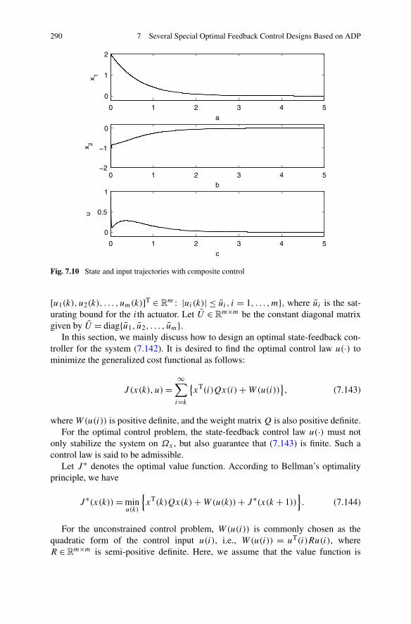
290 7 Several Special Optimal Feedback Control Designs Based on ADP
Fig. 7.10 State and input trajectories with composite control
[u1(k), u2(k), . . . , um(k)]T ∈ Rm : |ui(k)| ≤ ui , i = 1, . . . ,m}, where ui is the sat-
urating bound for the ith actuator. Let U ∈ Rm×m be the constant diagonal matrix
given by U = diag{u1, u2, . . . , um}.In this section, we mainly discuss how to design an optimal state-feedback con-
troller for the system (7.142). It is desired to find the optimal control law u(·) tominimize the generalized cost functional as follows:
J (x(k), u)=∞∑
i=k
{xT(i)Qx(i)+W(u(i))
}, (7.143)
where W(u(i)) is positive definite, and the weight matrix Q is also positive definite.For the optimal control problem, the state-feedback control law u(·) must not
only stabilize the system on Ωx , but also guarantee that (7.143) is finite. Such acontrol law is said to be admissible.
Let J ∗ denotes the optimal value function. According to Bellman’s optimalityprinciple, we have
J ∗(x(k))= minu(k)
{xT(k)Qx(k)+W(u(k))+ J ∗(x(k + 1))
}. (7.144)
For the unconstrained control problem, W(u(i)) is commonly chosen as thequadratic form of the control input u(i), i.e., W(u(i)) = uT(i)Ru(i), whereR ∈R
m×m is semi-positive definite. Here, we assume that the value function is
7.5 Optimal Feedback Control for a Class of Constrained Systems Via SNAC 291
smooth. According to the necessary condition for optimality, we obtain
u∗(k)= −1
2R−1gT(x(k))
∂J ∗(x(k + 1))
∂x(k + 1), (7.145)
where J ∗ is the optimal value function with respect to the optimal control law u∗.However, the above derivation is not suitable for constrained optimal control
problem. To guarantee bounded controls, inspired by [8], a nonquadratic functionalis introduced as follows:
W(u(i))= 2∫ u(i)
0ϕ−T(U−1s)URds,
ϕ−1(u(i))= [ϕ−1(u1(i)), . . . , ϕ−1(um(i))], (7.146)
where R is positive definite and assumed to be diagonal for simplicity of analysis,s ∈ R
m, ϕ ∈ Rm, ϕ(·) is a bounded one-to-one function satisfying |ϕ(·)| ≤ 1 and
belonging to Cp(p ≥ 1) and L2(Ωx). Moreover, it is a monotonically increasingodd function with its first derivative bounded by M . Such function is easy to find,and one example is the hyperbolic tangent function ϕ(·)= tanh(·). It should be no-ticed that by the definition above, W(u(i)) is ensured to be positive definite becauseϕ−1(·) is a monotonic odd function and R is positive definite.
Substituting (7.146) into (7.144), the HJB equation can be derived as follows:
J ∗(x(k))= minu(k)
{xT(k)Qx(k)+ 2
∫ u(k)
0ϕ−T(U−1s)URds + J ∗(x(k + 1))
}.
(7.147)
Assuming that the value function is smooth, and according to the necessary con-dition for optimality, we obtain
∂J ∗(x(k))∂u(k)
= 2RUϕ−1(U−1u(k))+(∂x(k + 1)
∂u(k)
)T ∂J ∗(x(k + 1))
∂x(k + 1)= 0. (7.148)
Therefore, letting J ∗x (x(k + 1)) = ∂J ∗(x(k + 1))/∂x(k + 1), the optimal control
law can be computed as follows:
u∗(k)= Uϕ
(−1
2(UR)−1gT(x(k))J ∗
x (x(k + 1))
). (7.149)
If the optimal value function J ∗ is known, the optimal control law u∗(k) canbe obtained from (7.149). However, there is currently no method for solving thisvalue function of the constrained optimal control problem. Therefore, in the nextsection we will discuss how to utilize the greedy iterative DHP algorithm to seekthe near-optimal control solution.
292 7 Several Special Optimal Feedback Control Designs Based on ADP
7.5.2 Optimal Controller Design for Constrained Systems viaSNAC
For convenience, in the sequel, W(u(k)) is used to denote the nonquadratic func-tional 2
∫ u(k)0 ϕ−T(U−1s)URds.
Define the costate function λ(x(k))= ∂J (x(k))∂x(k)
. Then, (7.149) can be rewritten as
u∗(k)= Uϕ(−1
2(UR)−1gT(x(k))λ∗(x(k + 1))
). (7.150)
By definition, the costate function λ∗(x(k)) satisfies
λ∗(x(k))= ∂J ∗(x(k))∂x(k)
= ∂(xT(k)Qx(k)+W(u(k)))
∂x(k)
+(∂u(x(k))
∂x(k)
)T∂(xT(k)Qx(k)+W(u(k)))
∂u(x(k))
+(∂x(k + 1)
∂x(k)
)T∂J ∗(x(k + 1))
∂x(k + 1)
+(∂u(x(k))
∂x(k)
)T(∂x(k + 1)
∂u(x(k))
)T∂J ∗(x(k + 1))
∂x(k + 1)
=(∂u(x(k))
∂x(k)
)T [∂(xT(k)Qx(k)+W(u(k)))
∂u(x(k))+(∂x(k + 1)
∂u(x(k))
)T
× ∂J ∗(x(k + 1))
∂x(k + 1)
]+ ∂(xT(k)Qx(k)+W(u(k)))
∂x(k)
+(∂x(k + 1)
∂x(k)
)T∂J ∗(x(k + 1))
∂x(k + 1)
= 2Qx(k)+(∂x(k + 1)
∂x(k)
)T
λ∗(x(k + 1)). (7.151)
The optimal control law can be solved from (7.150) if the costate function λ∗ canbe obtained from (7.151). However, it is very difficult to solve (7.151) analyticallydue to the two-point boundary value problems of partial difference equation. There-fore, a greedy iterative DHP algorithm is developed to obtain the costate functionλ∗ and the optimal control law u∗ in the sequel.
First, we start with initial value function V0(·) = 0 and initial costate functionλ0(·)= 0, Then, we find the law of single control vector v0 as follows:
v0(x(k))= arg minu(k)
{xT(k)Qx(k)+W(u(k))+ V0(x(k + 1))
}. (7.152)
7.5 Optimal Feedback Control for a Class of Constrained Systems Via SNAC 293
According to the optimal principle, v0(x) can be derived as follows:
v0(x(k))= Uϕ(−1
2(UR)−1gT(x(k))λ0(x(k + 1))
). (7.153)
Thus, we have
x(k + 1)= f (x(k))+ g(x(k))v0(x(k)), (7.154)
and
v0(x(k + 1))
= arg minu(k+1)
{xT(k + 1)Qx(k + 1)+W(u(k + 1))+ V0(x(k + 2))
}. (7.155)
According to λ0(x(k + 2)) = ∂V0(x(k + 2))/∂x(k + 2), and using (7.155), wehave
v0(x(k + 1))= Uϕ(−1
2(UR)−1gT(x(k + 1))λ0(x(k + 2))
). (7.156)
Then, the value function can be updated as
V1(x(k + 1))= xT(k + 1)Qx(k + 1)+W(v0(k + 1))+ V0(x(k + 2)). (7.157)
Therefore, for i = 0,1, . . . , the iterative ADP algorithm is realized by implementingthe iterations between
vi(x(k + 1))
= arg minu(k+1)
{xT(k + 1)Qx(k + 1)+W(u(k + 1))+ Vi(x(k + 2))
}(7.158)
and
Vi+1(x(k + 1))= minu(k+1)
{xT(k + 1)Qx(k + 1)+W(u(k + 1))+ Vi(x(k + 2))
}
= xT(k + 1)Qx(k + 1)+W(vi(k + 1))+ Vi(x(k + 2)) (7.159)
until convergence.Obviously, if we assume that the value function Vi is smooth, vi(k+1) in (7.158)
can further be solved as
∂Vi+1(x(k + 1))
∂v(k + 1)= ∂(xT(k + 1)Qx(k + 1)+W(vi(k + 1))
∂v(k + 1)
+ gT(x(k + 1))∂Vi(x(k + 2))
∂x(k + 2)
= 0. (7.160)
294 7 Several Special Optimal Feedback Control Designs Based on ADP
That is,
vi(k + 1)= Uϕ(−1
2(UR)−1gT(x(k + 1))λi(x(k + 2))
). (7.161)
Because λi+1(x(k + 1)) = ∂Vi+1(x(k + 1))/∂x(k + 1), similarly to the derivativeprocess of (7.151), we have
λi+1(x(k + 1))
= ∂(xT(k + 1)Qx(k + 1)+W(vi(k + 1)))
∂x(k + 1)
+(∂vi(x(k + 1))
∂x(k + 1)
)T∂(xT(k + 1)Qx(k + 1)+W(vi(k + 1)))
∂vi(x(k + 1))
+(∂x(k + 2)
∂x(k + 1)
)T∂Vi(x(k + 2))
∂x(k + 2)
+(∂vi(x(k + 1))
∂x(k + 1)
)T(∂x(k + 2)
∂vi(x(k + 1))
)T∂Vi(x(k + 2))
∂x(k + 2)
= ∂(xT(k + 1)Qx(k + 1)+W(vi(k + 1)))
∂x(k + 1)+ gT(x(k + 1))
∂Vi(x(k + 2))
∂x(k + 2).
(7.162)
That is,
λi+1(x(k + 1))= 2Qx(k + 1)+ gT(x(k + 1))λi(x(k + 2)). (7.163)
Therefore, we obtain the optimal control as follows:
vi(x(k))= Uϕ
(−1
2(UR)−1gT(x(k))λi(x(k + 1))
). (7.164)
Hence, the iteration between (7.158) and (7.159) is an implementation of the itera-tion between (7.163) and (7.164).
In the following, we present the convergence analysis of the greedy iterative DHPalgorithm. We first present two lemmas before presenting our theorems.
Lemma 7.22 Let μi be an arbitrary sequence of control laws, and vi be the controllaw sequence as in (7.158). Let Vi be as in (7.159) and Λi be
Λi+1(x(k + 1))= xT(k + 1)Qx(k + 1)+W(μi(k + 1))+Λi(x(k + 2)).(7.165)
If V0 =Λ0 = 0, then Vi ≤Λi , ∀i.
Lemma 7.23 Let {Vi} be defined as in(7.159). If the system is controllable, thenthere is an upper bound Y such that 0 ≤ Vi ≤ Y, ∀i.
7.5 Optimal Feedback Control for a Class of Constrained Systems Via SNAC 295
Proof Let η(x(k+1)) be a sequence of stabilizing and admissible control laws, andlet V0(·)= Z0(·)= 0, where Vi is updated by (7.159) and Zi is updated by
Zi+1(x(k + 1))= xT(k + 1)Qx(k + 1)+W(η(x(k + 1)))+Zi(x(k + 2)).(7.166)
Then, we obtain
Zi+1(x(k + 1))−Zi(x(k + 1))= Zi(x(k + 2))−Zi−1(x(k + 2))
= Zi−1(x(k + 3))−Zi−2(x(k + 3))
= Zi−2(x(k + 4))−Zi−3(x(k + 4))
...
= Z1(x(k + i + 1))−Z0(x(k + i + 1)). (7.167)
Thus, the following relation can be obtained:
Zi+1(x(k + 1))= Z1(x(k + i + 1))+Zi(x(k + 1))−Z0(x(k + i + 1)). (7.168)
Since Z0(·)= 0, it follows that
Zi+1(x(k + 1))= Z1(x(k + i + 1))+Zi(x(k + 1))
= Z1(x(k + i + 1))+Z1(x(k + i))+Zi−1(x(k + 1))
= Z1(x(k + i + 1))+Z1(x(k + i))
+Z1(x(k + i − 1))+ · · · +Z1(x(k + 1)). (7.169)
Then, (7.169) can further be rewritten as
Zi+1(x(k + 1))=i∑
j=0
Z1(x(k + j + 1))
=i∑
j=0
{xT(k + j + 1)Qx(k + j + 1)+W(η(x(k + j + 1)))
}
≤∞∑
j=0
{xT(k + j + 1)Qx(k + j + 1)+W(η(x(k + j + 1)))
}.
(7.170)
Note that η(x(k + 1)) is an admissible control law sequence, i.e., x(k + 1)→ 0as k → ∞, Therefore, there exists an upper bound Y such that
∀i : Zi+1(x(k + 1))≤∞∑
j=0
Z1(x(k + j + 1))≤ Y. (7.171)
296 7 Several Special Optimal Feedback Control Designs Based on ADP
Combining with Lemma 1, we obtain
∀i : Vi+1(x(k + 1))≤ Zi+1(x(k + 1))≤ Y. (7.172)
The proof is completed. �
Next, Lemmas 7.22 and 7.23 will be used in the proof of our main theorems.
Theorem 7.24 (cf. [6]) Define the value function sequence {Vi} as in (7.159) withV0 = 0, and the control law sequence {vi} as in (7.163). Then, we can conclude that{Vi} is a nondecreasing sequence satisfying Vi+1(x(k+ 1))≥ Vi(x(k+ 1)),∀i, andis convergent to the value function of the discrete-time HJB equation, i.e., Vi → J ∗as i → ∞. Meanwhile, we conclude that the costate function sequence {λi} and thecontrol law sequence {vi} are also convergent, i.e., λi → λ∗ and vi → u∗ as i → ∞.
Proof For convenience of analysis, define a new sequence Φ as follows:
Φi+1(x(k + 1))= xT(k + 1)Qx(k + 1)+W(vi+1(k + 1))+Φi(x(k + 2)),(7.173)
with Φ0 = V0 = 0. The control law sequence vi is updated by (7.158) and the valuefunction sequence Vi is updated by (7.159).
In the following, we prove that Φi(x(k + 1))≤ Vi+1(x(k + 1)) by mathematicalinduction.
First, we prove that it holds for i = 0. Noticing that
V1(x(k + 1))−Φ0(x(k + 1))= xT(k + 1)Qx(k + 1)+W(v0(k + 1))≥ 0,(7.174)
we have
V1(x(k + 1))≥Φ0(x(k + 1)). (7.175)
Second, we assume that it holds for i − 1, i.e., for any x(k + 1), Vi(x(k + 1))≥Φi−1(x(k + 1)). Then, for i, since
Φi(x(k + 1))= xT(k + 1)Qx(k + 1)+W(vi(k + 1))+Φi−1(x(k + 2)) (7.176)
and
Vi+1(x(k + 1))= xT(k + 1)Qx(k + 1)+W(vi(k + 1))+ Vi(x(k + 2)) (7.177)
hold, we obtain
Vi+1(x(k + 1))−Φi(x(k + 1))= Vi(x(k + 2))−Φi−1(x(k + 2))≥ 0, (7.178)
i.e., the following equation holds:
Φi(x(k + 1))≤ Vi+1(x(k + 1)). (7.179)
7.5 Optimal Feedback Control for a Class of Constrained Systems Via SNAC 297
Therefore, for ∀i, (7.179) is proved by mathematical induction.Furthermore, from Lemma 7.22, we know that Vi(x(k + 1)) ≤ Φi(x(k + 1)).
Therefore, we have
Vi(x(k + 1))≤Φi(x(k + 1))≤ Vi+1(x(k + 1)). (7.180)
Hence, we can conclude that the value function sequence {Vi} is a nondecreasingsequence satisfying Vi+1(x(k + 1))≥ Vi(x(k + 1)),∀i, and convergent to the opti-mal value function of the discrete-time HJB equation, i.e., Vi → J ∗ as i → ∞. Thecostate sequence {λi} is also convergent, i.e., λi → λ∗ as i → ∞.
Since the value function sequence and the costate function sequence are con-vergent, according to (7.163) and (7.164), we conclude that {vi} converges to theoptimal control law u∗ as i → ∞. �
For linear systems, if the cost functional is quadratic, then the optimal controllaw is linear. For nonlinear system, this is not true. So we use neural network toapproximate costate function, and get the optimal control law.
In this part, we use single network GI-DHP algorithm to obtain the optimalcostate function and optimal control law. SNAC can remove the action network ap-pearing in the ordinary ADP method. It simplifies the structure of the system, savesstorage space and reduces computation. In addition, it eliminates approximation er-ror of neural network, and improves the calculation accuracy. We have known thatthe control law is implicit function which is difficult to solve. So the costate func-tion should be transformed. As λ(x(k + 1)) can be expressed by x(k), so we letλ(x(k))= λ(x(k + 1)). Then, the critic neural network can be used to approximateλ(x(k)).
Equation (7.163) can be written as
λi+1(x(k))= 2Qx(k + 1)+ gT(x(k + 1))λi(x(k + 1)). (7.181)
The optimal control law can be obtained as follows:
vi(x(k))= Uϕ
(−1
2(UR)−1gT(x(k))λi (x(k))
). (7.182)
Once we get the costate function λ(x(k)), then according to (7.182), we canget the optimal control law. Let λ0(·) = 0, and then the iteration between (7.163)and (7.164) is changed into the iteration between (7.181) and (7.182).
Based on the above analysis, we give the structure in Fig. 7.11.For each iteration, we use three layer forward neural network to approximate
λi(x(k + 1))
λi(x(k + 1))= ˆλi(x(k))= wTi σ (v
Ti x(k)), (7.183)
where wi and vi is the weights of output and hidden layers, σ(·) ∈ Rl , [σ(z)]p =
ezp −e−zp
ezp +e−zp
, p = 1, . . . , l, is the activation function of hidden layer, and l is the numberas hidden node.
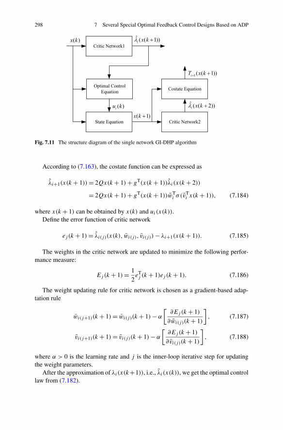
298 7 Several Special Optimal Feedback Control Designs Based on ADP
Fig. 7.11 The structure diagram of the single network GI-DHP algorithm
According to (7.163), the costate function can be expressed as
λi+1(x(k + 1))= 2Qx(k + 1)+ gT(x(k + 1))λi(x(k + 2))
= 2Qx(k + 1)+ gT(x(k + 1))wTi σ (v
Ti x(k + 1)), (7.184)
where x(k + 1) can be obtained by x(k) and ui(x(k)).Define the error function of critic network
ej (k + 1)= λi(j)(x(k), wi(j), vi(j))− λi+1(x(k + 1)). (7.185)
The weights in the critic network are updated to minimize the following perfor-mance measure:
Ej(k + 1)= 1
2eTj (k + 1)ej (k + 1). (7.186)
The weight updating rule for critic network is chosen as a gradient-based adap-tation rule
wi(j+1)(k + 1)= wi(j)(k + 1)− α
[∂Ej (k + 1)
∂wi(j)(k + 1)
], (7.187)
vi(j+1)(k + 1)= vi(j)(k + 1)− α
[∂Ej (k + 1)
∂vi(j)(k + 1)
], (7.188)
where α > 0 is the learning rate and j is the inner-loop iterative step for updatingthe weight parameters.
After the approximation of λi(x(k+1)), i.e., λi (x(k)), we get the optimal controllaw from (7.182).
7.5 Optimal Feedback Control for a Class of Constrained Systems Via SNAC 299
7.5.3 Simulations
In this section, two examples are provided to demonstrate the effectiveness of thecontrol scheme.
Example 7.25 Consider the following Van der Pol oscillator system in [9]:
x1 = x2,
x2 = α(1 − x21)x2 − x1 + (1 + x2
1 + x22)u, (7.189)
where α = 0.05, control constraint is set to |u| ≤ 0.2.We first use the Euler method to discretize the system, where t = kT , T is sam-
pling period, k is sampling step. If T is small enough compared with the systemtime constant, then the discretization method is precise enough.
So, let T = 0.1; we have
x1(k + 1)= x1(k)+ 0.1x2(k),
x2(k + 1)= −x1(k)+ 0.005(1 − x21(k))x2(k)+ x2(k)
+ (1 + x21(k)+ x2
2(k))u(k). (7.190)
Define the cost functional as
J (x(k), u)=∞∑
i=k
{xT(i)Qx(i)+ 2U
∫ u(i)
0tanh−T(Us)Rds
}, (7.191)
where U = 0.2 and Q= [ 3 00 3
], R = [ 2 ].
We choose neural networks as the critic network with the structures 2–9–2. Theinitial weights of the output layer are zero to guarantee the initial output of criticnetwork is zero, i.e., λ0 = 0. The initial weights of the hidden layer are chosen ran-domly in [−1 1]. We train the critic network for 1200 iteration steps and 2000 timesteps. The critic network is trained until the given accuracy 10−10. The convergencecurves of the costate function are shown in Fig. 7.12. Furthermore, for x1(0)= 0.1and x2(0)= 0.3, we run the system for 200 time steps, we get the state trajectory inFig. 7.13 and control trajectory in Fig. 7.14.
Moreover, in order to make comparison with the controller designed withoutconsidering the actuator saturation, we also present the system responses obtainedby the controller designed regardless of the actuator saturation. After simulation, thestate curves is shown in Fig. 7.15 and the control curve is shown in Fig. 7.16.
From the simulation results, we can see that the iterative costate function se-quences do converge to the optimal ones with very fast speed, which also indicatesthe validity of the iterative ADP algorithm for dealing with constrained nonlinearsystems.
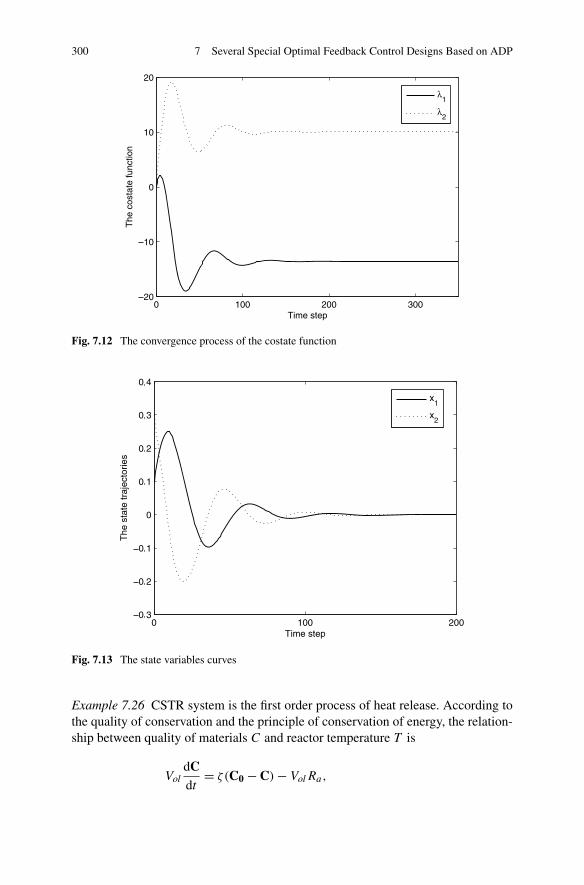
300 7 Several Special Optimal Feedback Control Designs Based on ADP
Fig. 7.12 The convergence process of the costate function
Fig. 7.13 The state variables curves
Example 7.26 CSTR system is the first order process of heat release. According tothe quality of conservation and the principle of conservation of energy, the relation-ship between quality of materials C and reactor temperature T is
VoldCdt
= ζ(C0 − C)− VolRa,
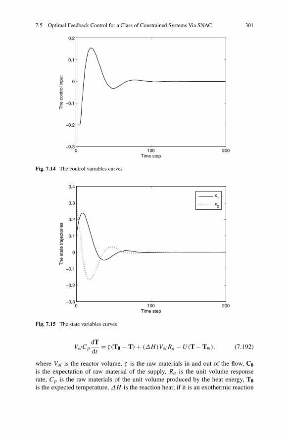
7.5 Optimal Feedback Control for a Class of Constrained Systems Via SNAC 301
Fig. 7.14 The control variables curves
Fig. 7.15 The state variables curves
VolCp
dTdt
= ζ(T0 − T)+ (ΔH)VolRa −U(T − Tw), (7.192)
where Vol is the reactor volume, ζ is the raw materials in and out of the flow, C0is the expectation of raw material of the supply, Ra is the unit volume responserate, Cp is the raw materials of the unit volume produced by the heat energy, T0is the expected temperature, ΔH is the reaction heat; if it is an exothermic reaction
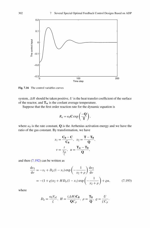
302 7 Several Special Optimal Feedback Control Designs Based on ADP
Fig. 7.16 The control variables curves
system, ΔH should be taken positive, U is the heat transfer coefficient of the surfaceof the reactor, and Tw is the coolant average temperature.
Suppose that the first order reaction rate for the dynamic equation is
Ra = κ0C exp
(−QT
),
where κ0 is the rate constant, Q is the Arrhenius activation energy and we have theratio of the gas constant. By transformation, we have
x1 = C0 − CC0
, x2 = T − T0
Q,
ν = t
Volζ
, u= Tw − T0
Q,
and then (7.192) can be written as
dx1
dν= −x1 +Da(1 − x1) exp
(− 1
x2 + ρ
)dx2
dν
= −(1 + �)x2 +HDa(1 − x1) exp
(− 1
x2 + ρ
)+ �u, (7.193)
where
Da = κ0Vol
ζ, H = (ΔH)C0
QCp
, ρ = T0
Q, � = U
ζCp
.
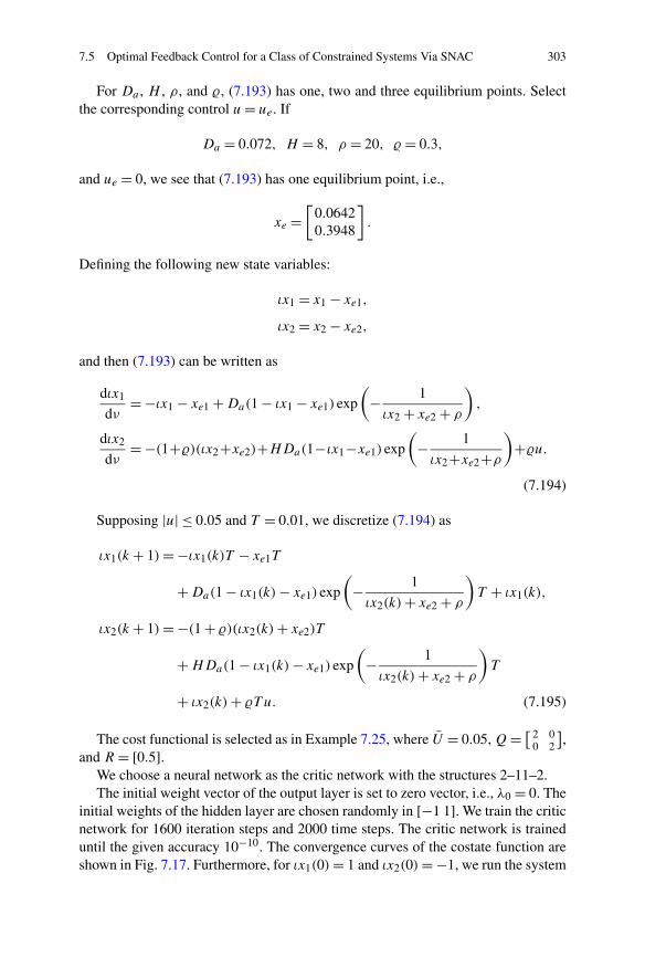
7.5 Optimal Feedback Control for a Class of Constrained Systems Via SNAC 303
For Da , H , ρ, and �, (7.193) has one, two and three equilibrium points. Selectthe corresponding control u= ue. If
Da = 0.072, H = 8, ρ = 20, � = 0.3,
and ue = 0, we see that (7.193) has one equilibrium point, i.e.,
xe =[
0.06420.3948
].
Defining the following new state variables:
ιx1 = x1 − xe1,
ιx2 = x2 − xe2,
and then (7.193) can be written as
dιx1
dν= −ιx1 − xe1 +Da(1 − ιx1 − xe1) exp
(− 1
ιx2 + xe2 + ρ
),
dιx2
dν= −(1+�)(ιx2+xe2)+HDa(1−ιx1−xe1) exp
(− 1
ιx2+xe2+ρ
)+�u.
(7.194)
Supposing |u| ≤ 0.05 and T = 0.01, we discretize (7.194) as
ιx1(k + 1)= −ιx1(k)T − xe1T
+Da(1 − ιx1(k)− xe1) exp
(− 1
ιx2(k)+ xe2 + ρ
)T + ιx1(k),
ιx2(k + 1)= −(1 + �)(ιx2(k)+ xe2)T
+HDa(1 − ιx1(k)− xe1) exp
(− 1
ιx2(k)+ xe2 + ρ
)T
+ ιx2(k)+ �T u. (7.195)
The cost functional is selected as in Example 7.25, where U = 0.05, Q= [ 2 00 2
],
and R = [0.5].We choose a neural network as the critic network with the structures 2–11–2.The initial weight vector of the output layer is set to zero vector, i.e., λ0 = 0. The
initial weights of the hidden layer are chosen randomly in [−1 1]. We train the criticnetwork for 1600 iteration steps and 2000 time steps. The critic network is traineduntil the given accuracy 10−10. The convergence curves of the costate function areshown in Fig. 7.17. Furthermore, for ιx1(0)= 1 and ιx2(0)= −1, we run the system
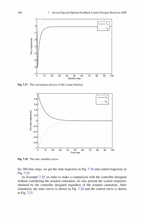
304 7 Several Special Optimal Feedback Control Designs Based on ADP
Fig. 7.17 The convergence process of the costate function
Fig. 7.18 The state variables curves
for 100 time steps, we get the state trajectory in Fig. 7.18 and control trajectory inFig. 7.19.
As Example 7.25, in order to make a comparison with the controller designedwithout considering the actuator saturation, we also present the system responsesobtained by the controller designed regardless of the actuator saturation. Aftersimulation, the state curves is shown in Fig. 7.20 and the control curve is shownin Fig. 7.21.
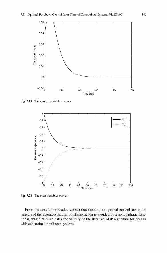
7.5 Optimal Feedback Control for a Class of Constrained Systems Via SNAC 305
Fig. 7.19 The control variables curves
Fig. 7.20 The state variables curves
From the simulation results, we see that the smooth optimal control law is ob-tained and the actuators saturation phenomenon is avoided by a nonquadratic func-tional, which also indicates the validity of the iterative ADP algorithm for dealingwith constrained nonlinear systems.
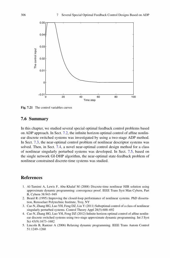
306 7 Several Special Optimal Feedback Control Designs Based on ADP
Fig. 7.21 The control variables curves
7.6 Summary
In this chapter, we studied several special optimal feedback control problems basedon ADP approach. In Sect. 7.2, the infinite horizon optimal control of affine nonlin-ear discrete switched systems was investigated by using a two-stage ADP method.In Sect. 7.3, the near-optimal control problem of nonlinear descriptor systems wassolved. Then, in Sect. 7.4, a novel near-optimal control design method for a classof nonlinear singularly perturbed systems was developed. In Sect. 7.5, based onthe single network GI-DHP algorithm, the near-optimal state-feedback problem ofnonlinear constrained discrete-time systems was studied.
References
1. Al-Tamimi A, Lewis F, Abu-Khalaf M (2008) Discrete-time nonlinear HJB solution usingapproximate dynamic programming: convergence proof. IEEE Trans Syst Man Cybern, PartB, Cybern 38:943–949
2. Beard R (1995) Improving the closed-loop performance of nonlinear systems. PhD disserta-tion, Rensselaer Polytechnic Institute, Troy, NY
3. Cao N, Zhang HG, Luo YH, Feng DZ, Liu Y (2011) Suboptimal control of a class of nonlinearsingularly perturbed systems. Control Theory Appl 28(5):688–692
4. Cao N, Zhang HG, Luo YH, Feng DZ (2012) Infinite horizon optimal control of affine nonlin-ear discrete switched systems using two-stage approximate dynamic programming. Int J SystSci 43(9):1673–1682
5. Lincoln B, Rantzer A (2006) Relaxing dynamic programming. IEEE Trans Autom Control51:1249–1260
References 307
6. Luo YH, Zhang HG, Cao N, Chen B (2009) Near-optimal stabilization for a class of nonlinearsystems with control constraint based on single network greedy iterative DHP algorithm. ActaAutom Sin 35(11):1436–1445
7. Luo YH, Liu Z, Yang D (2010) Greedy iterative DHP algorithm-based near-optimal controlfor a class of nonlinear descriptor systems with actuator saturating. In: Proceedings of the 9thIEEE international conference on cognitive informatics, pp 788–793
8. Lyshevski SE (1998) Nonlinear discrete-time systems: constrained optimization and applica-tion of nonquadratic costs. In: Proceedings of the American control conference, Philadelphia,USA, pp 3699–3703
9. Padhi R, Unnikrishnan N, Wang X, Balakrishnan SN (2006) A single network adaptive critic(SNAC) architecture for optimal control synthesis for a class of nonlinear systems. NeuralNetw 19(10):1648–1660
10. Rantzer A (2005) On approximate dynamic programming in switching systems. In: Proceed-ing of the IEEE conference on decision and control and the European control conference,Seville, Spain, pp 1391–1396
11. Seatzu C, Corona D, Giua A, Bempoard A (2006) Optimal control of continuous time switchedaffine systems. IEEE Trans Autom Control 51:726–741
12. Xu XP, Antsaklis PJ (2000) Optimal control of switched systems: new results and open prob-lems. In: Proceeding of the American control conference, Chicago, Illinois, pp 2683–2687
13. Xu XP, Antsaklis PJ (2003) Results and perspectives on computational methods for optimalcontrol of switched systems. Hybrid systems: computation and control (HSCC). Springer,Berlin, pp 540–555
14. Yang H, Jiang B, Cocquempot V, Zhang HG (2011) Stabilization of switched nonlinear sys-tems with all unstable modes: application to multi-agent systems. IEEE Trans Autom Control56(9):2230–2235
15. Zhang W, Hu J, Abate A (2009) On the value functions of the discrete-time switched LQRproblem. IEEE Trans Autom Control 54:2669–2674
16. Zhang HG, Liu Z, Huang GB (2010) Novel delay-dependent robust stability analysis forswitched neutral-type neural network with time-varying delays via SC technique. IEEE TransSyst Man Cybern, Part B, Cybern 40(6):1480–1491
Chapter 8Zero-Sum Games for Discrete-Time SystemsBased on Model-Free ADP
8.1 Introduction
A large class of complicated practical systems are controlled by more than onecontroller or decision maker, each using an individual strategy. These controllersoften operate in a group with a general cost functional as a game [8, 11]. Zero-sum game theory has been widely applied to decision making and control engi-neering problems [7]. Recently, much work has been done in the area of dealingwith zero-sum games based on ADP methods [2–6], most of which are only for theone-dimensional systems. In the real world, many complicated control systems aredescribed by 2-dimensional (2-D) structures [12, 15], such as thermal processes, im-age processing, signal filtering, etc. However, the optimal recurrent equation, the socalled Hamilton–Jacobi–Isaacs (HJI) equation, is invalid in the 2-D structure. More-over, the exact models of many 2-D systems cannot be obtained inherently. To solvethe aforementioned problems, in Sect. 8.2, we will study the zero-sum games for aclass of discrete-time Roesser types 2-D systems based on model-free ADP method.First, we will propose the optimality principle for 2-D systems and obtain the ex-pressions of optimal control pair for the zero-sum games. Then, a data-based itera-tive ADP algorithm is developed without the requirement of the exact system model.
It is well known that some states of the system may not be measurable in manypractical situations. So it is desirable to use available input–output data, rather thanthe states of system in the design of controller. In Sect. 8.3, we will develop a noveldata-based optimal output feedback control scheme via the ADP algorithm, in whichneither the exact system model nor the full states of the system are needed.
8.2 Zero-Sum Differential Games for a Class of Discrete-Time2-D Systems
In this section, we will use the model-free ADP method to obtain the optimal controlpair iteratively which makes the performance index function reach the saddle pointof the zero-sum games for a class of discrete-time 2-D systems.
H. Zhang et al., Adaptive Dynamic Programming for Control,Communications and Control Engineering, DOI 10.1007/978-1-4471-4757-2_8,© Springer-Verlag London 2013
309
310 8 Zero-Sum Games for Discrete-Time Systems Based on Model-Free ADP
8.2.1 Problem Formulation
Basically, we consider the following discrete-time linear Roesser type 2-D systems:
x+(k, l)=Ax(k, l)+Bu(k, l)+Cw(k, l) (8.1)
xh(0, l)= f (l), xv(k,0)= g(k) (8.2)
with
x(k, l)=[xh(k, l)
xv(k, l)
], x+(k, l)=
[xh(k + 1, l)xv(k, l + 1)
], (8.3)
where xh(k, l) is the horizontal state in Rn1 , xv(k, l) is the vertical state in R
n2 ,u(k, l) and w(k, l) are the control input in R
m1 and Rm2 . Let the system matrices be
A ∈ R(n1+n2)×(n1+n2), B ∈ R
(n1+n2)×n1 , and C ∈R(n1+n2)×m2 . It is assumed that all
the system matrices are nonsingular, and that the system matrices can be expressedby
A=[A1 A2A3 A4
], B =
[B1B2
], C =
[C1C2
]. (8.4)
The functions f (l) and g(k) are the corresponding boundary conditions along twoindependent directions.
We define the following notation:
(k, l)≤ (m,n) if and only if k ≤m and l ≤ n,
(k, l)= (m,n) if and only if k =m and l = n,
(k, l) < (m,n) if and only if (k, l)≤ (m,n) and
(k, l) �= (m,n). (8.5)
Then, the infinite-time cost functional for the 2-D system (8.1) is given by
J (x(0,0), u,w)=∑∑
(0,0)≤(k,l)<(∞,∞)
(xT(k, l)Qx(k, l)
+uT(k, l)Ru(k, l)+wT(k, l)Sw(k, l)), (8.6)
where Q≥ 0, R > 0, and S < 0 have suitable dimensions, and L(x(k, l), u(k, l))=xT(k, l)Qx(k, l) + uT(k, l)Ru(k, l) + wT(k, l)Sw(k, l) is the utility function. Forthe above zero-sum game, the two control variables u and w are chosen, respec-tively, by player I and player II, where player I tries to minimize the cost functionalJ (x(0,0), u,w), while player II attempts to maximize it. The following assump-tions are needed; they are in effect in the remaining sections.
8.2 Zero-Sum Differential Games for a Class of Discrete-Time 2-D Systems 311
Assumption 8.1 The 2-D system (8.1) is controllable under the control variables uand w.
Assumption 8.2 For the boundary conditions of the 2-D system (8.1), the terms∑∞k=0 x
vT(k,0)xv(k,0),∑∞
l=0 xhT(0, l)xh(0, l) and
∑∑
(0,0)≤(k,l)<(∞,∞)
xvT(k,0)xh(0, l)
are all bounded.
Assumption 8.3 There exists a unique saddle point of the zero-sum games for the2-D system (8.1).
There are some important characteristics that must be pointed out. First, forthe 1-D control system, the boundary condition is just an initial point of state,while the boundary conditions of 2-D system are two given state trajectoriesalong two different directions. Second, for the zero-sum games of 2-D systemunder the infinite time horizon, the boundary state trajectories are uncontrol-lable, and therefore the terms
∑∞l=0 x
T(k,0)Qx(k,0),∑∞
l=0 xT(0, l)Qx(0, l) and∑∑
(0,0)≤(k,l)<(∞,∞) xT(k,0)Qx(0, l) may be infinite, which means that the cost
functional (8.6) is infinite. Therefore, Assumption 8.2 is necessary. Third, theboundary conditions f (l) and g(k) in (8.2) should be boundary, but not necessarysmooth or continuous functions. For example, let
f (l)={c l ≤ T,
0 l > T,(8.7)
where c is any real constant number and T is given real number. So Assumption 8.2is not very strong.
According to Assumption 8.3, the optimal value function can be expressed as
J ∗(x(k, l))= minu
maxw
∑∑
(k,l)≤(i,j)<(∞,∞)
{xT(i, j)Qx(i, j)
+uT(i, j)Ru(i, j)+wT(i, j)Sw(i, j)}
= maxw
minu
∑∑
(k,l)≤(i,j)<(∞,∞)
{xT(i, j)Qx(i, j)
+uT(i, j)Ru(i, j)+wT(i, j)Sw(i, j)}. (8.8)
For the zero-sum games for 1-D systems, the optimal value function can be writ-ten by a recurrent formulation according to the dynamic programming principle.However, for the zero-sum games for 2-D systems, the dynamic programming prin-ciple may not be true. The main difficulty lies in the state of the 2-D system in
312 8 Zero-Sum Games for Discrete-Time Systems Based on Model-Free ADP
the next stage coupling with the states of two different directions in the currentstage; then the dynamic programming equation of the zero-sum games for 2-D sys-tems does not exist. So in this section, we propose an optimality principle for the2-D system and obtain the expressions of an optimal control pair for the zero-sumgames.
In the following, we will propose the optimality principle for the zero-sum gamesfor 2-D systems, and discuss the properties of the optimal control pair derived bythe optimality principle.
Theorem 8.4 (cf. [16]) If the cost functional is defined as (8.6), let u(k, l) minimizethe cost functional (8.6) and w(k, l) maximize it subject to the system equation (8.1);then there are (n+m)-dimensional vector sequences λ(k, l) and λ+(k, l) defined as
λ+(k, l)=[λh(k + 1, l)λv(k, l + 1)
], λ(k, l)=
[λh(k, l)
λv(k, l)
], (8.9)
where λh(k, l) ∈ Rn1 , λv(k, l) ∈ R
n2 , such that for all (0,0) ≤ (k, l) < (∞,∞) wehave the
1. State equation:
x+(k, l)= ∂H(k, l)
∂λ+(k, l), (8.10)
2. Costate equation:
λ(k, l)= ∂H(k, l)
∂x(k, l), (8.11)
3. Stationarity equation:
0 = ∂H(k, l)
∂u(k, l),
0 = ∂H(k, l)
∂w(k, l), (8.12)
where H(k, l) is a Hamilton function defined as
H(k, l)= xT(k, l)Qx(k, l)+ uT(k, l)Ru(k, l)
+wT(k, l)Sw(k, l)+ λ+T(k, l)(Ax(k, l)
+Bu(k, l)+Cw(k, l)). (8.13)
Proof By examining the gradients of each of the state equations, i.e., the vector ofpartial derivatives with respect to all the variables x(k, l), u(k, l), and w(k, l) ap-pearing in (8.6), they are easily seen to be linearly independent. The optimum ofthe cost functional (8.6) is therefore a regular point of the system (8.1) (see [13],
8.2 Zero-Sum Differential Games for a Class of Discrete-Time 2-D Systems 313
pp. 187). The existence of linear independent λ(k, l), (0,0)≤ (k, l) < (∞,∞) im-mediately follows from Lagrange multiplier theory (see [13], pp.187–198).
Let
J ′(x(k, l), u,w)=∑∑
(k,l)≤(i,j)<(∞,∞)
{xT(i, j)Qx(i, j)
+uT(i, j)Ru(i, j)+wT(i, j)Sw(i, j)
+λ+T(i, j)(Ax(i, j)+Bu(i, j)+Cw(i, j)
−x+(i, j))}. (8.14)
We introduce the Hamilton function of (8.13) and rewrite (8.14) as
J ′(x(k, l), u,w)=∑∑
(k,l)≤(i,j)<(∞,∞)
{H(i, j)− λ+T(i, j)x+(i, j)
}. (8.15)
The last term in the previous double summation can be expanded as follows:∑∑
(k,l)≤(i,j)<(∞,∞)
λ+T(i, j)x+(i, j)
=∑∑
(k,l)≤(i,j)<(∞,∞)
[λT(i, j)x(i, j)−
∞∑
j=l
λhT(0, j)xh(0, j)
−∞∑
i=k
λvT(i,0)xh(i,0)
]. (8.16)
According to the Lagrange multiplier theory, the increment J ′ due to incrementsin all x(k, l), u(k, l), w(k, l), and λ(k, l) must be zero at a constrained minimum.Hence
dJ ′(x(k, l), u,w)=∑∑
(k,l)≤(i,j)<(∞,∞)
{[∂H(i, j)
∂u(i, j)
]du(i, j)
+[∂H(i, j)
∂w(i, j)
]dw(i, j)
+[∂H(i, j)
∂λ+(i, j)− x+(i, j)
]dλ+(i, j)
+[∂H(i, j)
∂x(i, j)− λ(i, j)
]dx(i, j)
}. (8.17)
Equation (8.17) yields (8.10)–(8.12) by the following remarks:
1. Increments du(i, j), dw(i, j), dx(i, j), and dλ(i, j), with the exception ofdxh(0, j) and dxv(i,0), are independent arbitrary vectors.
314 8 Zero-Sum Games for Discrete-Time Systems Based on Model-Free ADP
2. dxh(0, j)= 0, dxv(i,0)= 0, since xh(i, j) and xv(i, j) are fixed boundary con-ditions. �
According to (8.12), the optimal control u∗(k, l) and w∗(k, l) can be expressedas
u∗(k, l)= −1
2R−1BTλ+(k, l), (8.18)
and
w∗(k, l)= −1
2S−1CTλ+(k, l). (8.19)
Theorem 8.5 (cf. [16]) For the system (8.1) with respect to the cost functional (8.6),if the controls u(k, l) and w(k, l) are expressed as (8.18) and (8.19) respectively,then the optimal Hamilton function (8.13) satisfies a certain Riccati function.
Proof For the zero-sum games of 2-D linear system, the optimal state feedbackcontrol should also be linearly dependent on the system state. As the system functionis time-invariant, there exists a matrix P that satisfies
λ(k, l)= 2Px(k, l). (8.20)
Then (8.18) and (8.19) can be rewritten as
u∗(k, l)= −BTP(Ax(k, l)+Bu(k, l)+Cw(k, l)), (8.21)
and
w∗(k, l)= −CTP(Ax(k, l)+Bu(k, l)+Cw(k, l)). (8.22)
So the optimal state feedback control u(k, l) and w(k, l) can be expressed as
u∗(k, l)= −(R +BTPB −BTPC(S +CTPC)−1CTPB)−1
× (BTPA−BTPC(S +CTPC)−1CTPA)x(k, l), (8.23)
and
w∗(k, l)= −(S +CTPC −CTPB(R +BTPB)−1BTPC)−1
× (CTPA−CTPB(R +BTPB)−1BTPA)x(k, l). (8.24)
According to (8.11) we have
2Px(k, l)= 2Qx(k, l)+ 2ATPx+(k, l)
= 2Qx(k, l)+ 2ATP(Ax(k, l)+Bu∗(k, l)
+Cw∗(k, l)). (8.25)
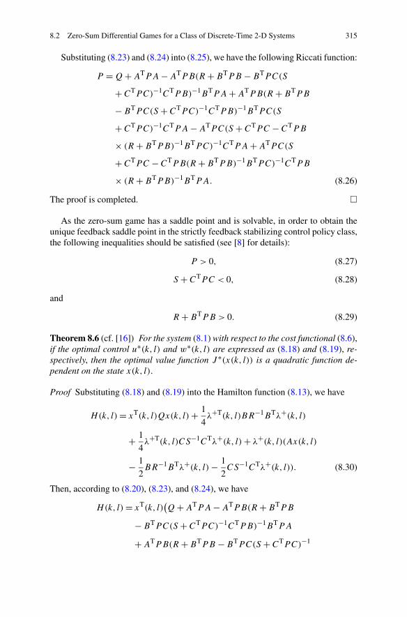
8.2 Zero-Sum Differential Games for a Class of Discrete-Time 2-D Systems 315
Substituting (8.23) and (8.24) into (8.25), we have the following Riccati function:
P =Q+ATPA−ATPB(R +BTPB −BTPC(S
+CTPC)−1CTPB)−1BTPA+ATPB(R +BTPB
−BTPC(S +CTPC)−1CTPB)−1BTPC(S
+CTPC)−1CTPA−ATPC(S +CTPC −CTPB
× (R +BTPB)−1BTPC)−1CTPA+ATPC(S
+CTPC −CTPB(R +BTPB)−1BTPC)−1CTPB
× (R +BTPB)−1BTPA. (8.26)
The proof is completed. �
As the zero-sum game has a saddle point and is solvable, in order to obtain theunique feedback saddle point in the strictly feedback stabilizing control policy class,the following inequalities should be satisfied (see [8] for details):
P > 0, (8.27)
S +CTPC < 0, (8.28)
and
R +BTPB > 0. (8.29)
Theorem 8.6 (cf. [16]) For the system (8.1) with respect to the cost functional (8.6),if the optimal control u∗(k, l) and w∗(k, l) are expressed as (8.18) and (8.19), re-spectively, then the optimal value function J ∗(x(k, l)) is a quadratic function de-pendent on the state x(k, l).
Proof Substituting (8.18) and (8.19) into the Hamilton function (8.13), we have
H(k, l)= xT(k, l)Qx(k, l)+ 1
4λ+T(k, l)BR−1BTλ+(k, l)
+ 1
4λ+T(k, l)CS−1CTλ+(k, l)+ λ+(k, l)(Ax(k, l)
− 1
2BR−1BTλ+(k, l)− 1
2CS−1CTλ+(k, l)). (8.30)
Then, according to (8.20), (8.23), and (8.24), we have
H(k, l)= xT(k, l)(Q+ATPA−ATPB(R +BTPB
−BTPC(S +CTPC)−1CTPB)−1BTPA
+ATPB(R +BTPB −BTPC(S +CTPC)−1
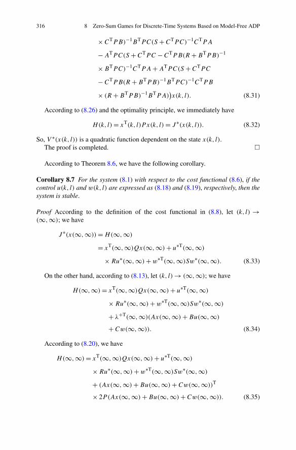
316 8 Zero-Sum Games for Discrete-Time Systems Based on Model-Free ADP
×CTPB)−1BTPC(S +CTPC)−1CTPA
−ATPC(S +CTPC −CTPB(R +BTPB)−1
×BTPC)−1CTPA+ATPC(S +CTPC
−CTPB(R +BTPB)−1BTPC)−1CTPB
× (R +BTPB)−1BTPA))x(k, l). (8.31)
According to (8.26) and the optimality principle, we immediately have
H(k, l)= xT(k, l)P x(k, l)= J ∗(x(k, l)). (8.32)
So, V ∗(x(k, l)) is a quadratic function dependent on the state x(k, l).The proof is completed. �
According to Theorem 8.6, we have the following corollary.
Corollary 8.7 For the system (8.1) with respect to the cost functional (8.6), if thecontrol u(k, l) and w(k, l) are expressed as (8.18) and (8.19), respectively, then thesystem is stable.
Proof According to the definition of the cost functional in (8.8), let (k, l) →(∞,∞); we have
J ∗(x(∞,∞))=H(∞,∞)
= xT(∞,∞)Qx(∞,∞)+ u∗T(∞,∞)
×Ru∗(∞,∞)+w∗T(∞,∞)Sw∗(∞,∞). (8.33)
On the other hand, according to (8.13), let (k, l)→ (∞,∞); we have
H(∞,∞)= xT(∞,∞)Qx(∞,∞)+ u∗T(∞,∞)
×Ru∗(∞,∞)+w∗T(∞,∞)Sw∗(∞,∞)
+ λ+T(∞,∞)(Ax(∞,∞)+Bu(∞,∞)
+Cw(∞,∞)). (8.34)
According to (8.20), we have
H(∞,∞)= xT(∞,∞)Qx(∞,∞)+ u∗T(∞,∞)
×Ru∗(∞,∞)+w∗T(∞,∞)Sw∗(∞,∞)
+ (Ax(∞,∞)+Bu(∞,∞)+Cw(∞,∞))T
× 2P(Ax(∞,∞)+Bu(∞,∞)+Cw(∞,∞)). (8.35)
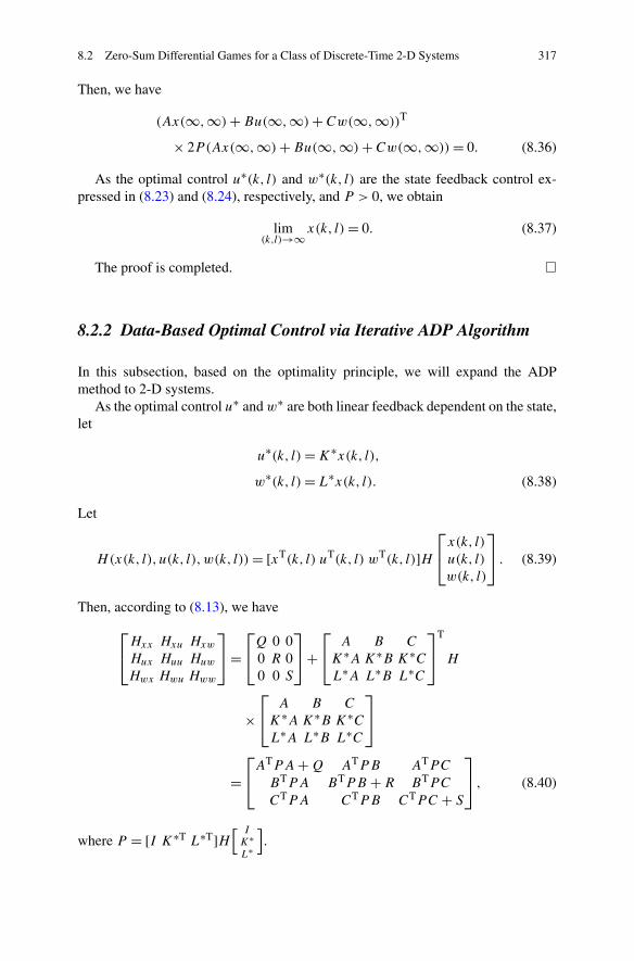
8.2 Zero-Sum Differential Games for a Class of Discrete-Time 2-D Systems 317
Then, we have
(Ax(∞,∞)+Bu(∞,∞)+Cw(∞,∞))T
× 2P(Ax(∞,∞)+Bu(∞,∞)+Cw(∞,∞))= 0. (8.36)
As the optimal control u∗(k, l) and w∗(k, l) are the state feedback control ex-pressed in (8.23) and (8.24), respectively, and P > 0, we obtain
lim(k,l)→∞x(k, l)= 0. (8.37)
The proof is completed. �
8.2.2 Data-Based Optimal Control via Iterative ADP Algorithm
In this subsection, based on the optimality principle, we will expand the ADPmethod to 2-D systems.
As the optimal control u∗ and w∗ are both linear feedback dependent on the state,let
u∗(k, l)=K∗x(k, l),
w∗(k, l)= L∗x(k, l). (8.38)
Let
H(x(k, l), u(k, l),w(k, l))= [xT(k, l) uT(k, l) wT(k, l)]H⎡
⎣x(k, l)
u(k, l)
w(k, l)
⎤
⎦ . (8.39)
Then, according to (8.13), we have
⎡
⎣Hxx Hxu Hxw
Hux Huu Huw
Hwx Hwu Hww
⎤
⎦=⎡
⎣Q 0 00 R 00 0 S
⎤
⎦+⎡
⎣A B C
K∗A K∗B K∗CL∗A L∗B L∗C
⎤
⎦T
H
×⎡
⎣A B C
K∗A K∗B K∗CL∗A L∗B L∗C
⎤
⎦
=⎡
⎣ATPA+Q ATPB ATPC
BTPA BTPB +R BTPC
CTPA CTPB CTPC + S
⎤
⎦ , (8.40)
where P = [I K∗T L∗T]H[ IK∗L∗
].
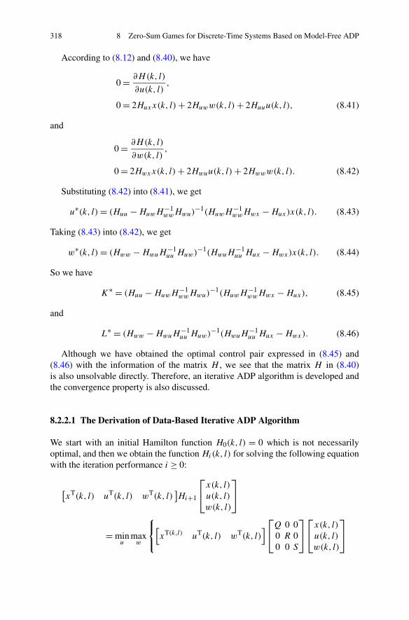
318 8 Zero-Sum Games for Discrete-Time Systems Based on Model-Free ADP
According to (8.12) and (8.40), we have
0 = ∂H(k, l)
∂u(k, l),
0 = 2Huxx(k, l)+ 2Huww(k, l)+ 2Huuu(k, l), (8.41)
and
0 = ∂H(k, l)
∂w(k, l),
0 = 2Hwxx(k, l)+ 2Hwuu(k, l)+ 2Hwww(k, l). (8.42)
Substituting (8.42) into (8.41), we get
u∗(k, l)= (Huu −HuwH−1wwHwu)
−1(HuwH−1wwHwx −Hux)x(k, l). (8.43)
Taking (8.43) into (8.42), we get
w∗(k, l)= (Hww −HwuH−1uu Huw)
−1(HwuH−1uu Hux −Hwx)x(k, l). (8.44)
So we have
K∗ = (Huu −HuwH−1wwHwu)
−1(HuwH−1wwHwx −Hux), (8.45)
and
L∗ = (Hww −HwuH−1uu Huw)
−1(HwuH−1uu Hux −Hwx). (8.46)
Although we have obtained the optimal control pair expressed in (8.45) and(8.46) with the information of the matrix H , we see that the matrix H in (8.40)is also unsolvable directly. Therefore, an iterative ADP algorithm is developed andthe convergence property is also discussed.
8.2.2.1 The Derivation of Data-Based Iterative ADP Algorithm
We start with an initial Hamilton function H0(k, l) = 0 which is not necessarilyoptimal, and then we obtain the function Hi(k, l) for solving the following equationwith the iteration performance i ≥ 0:
[xT(k, l) uT(k, l) wT(k, l)
]Hi+1
⎡
⎣x(k, l)
u(k, l)
w(k, l)
⎤
⎦
= minu
maxw
⎧⎨
⎩
[xT(k,l) uT(k, l) wT(k, l)
]⎡
⎣Q 0 00 R 00 0 S
⎤
⎦
⎡
⎣x(k, l)
u(k, l)
w(k, l)
⎤
⎦
8.2 Zero-Sum Differential Games for a Class of Discrete-Time 2-D Systems 319
+ [xT(k, l) uT(k, l) wT(k, l)
]⎡
⎣A B C
KA KB KC
LA LB LC
⎤
⎦T
Hi
×⎡
⎣A B C
KA KB KC
LA L∗B LC
⎤
⎦
⎡
⎣x(k, l)
u(k, l)
w(k, l)
⎤
⎦
⎫⎬
⎭
= [xT(k, l) uT
i (k, l) wTi (k, l)
]⎡
⎣Q 0 00 R 00 0 S
⎤
⎦
⎡
⎣x(k, l)
ui(k, l)
wi(k, l)
⎤
⎦
+ [xT(k, l) uT
i (k, l) wTi (k, l)
]⎡
⎣A B C
KiA KiB KiC
LiA LiB LiC
⎤
⎦T
Hi
×⎡
⎣A B C
KiA KiB KiC
LiA LiB LiC
⎤
⎦
⎡
⎣x(k, l)
ui(k, l)
wi(k, l)
⎤
⎦ . (8.47)
Then, according to (8.43) and (8.44), the iterative control laws can be expressed as
Ki = (H [i]uu −H [i]
uw(H[i]ww)
−1H [i]wu)
−1(H [i]uw(H
[i]ww)
−1H [i]wx −H [i]
ux ), (8.48)
and
Li = (H [i]ww −H [i]
wu(H[i]uu )
−1H [i]uw)
−1(H [i]wu(H
[i]uu )
−1H [i]ux −H [i]
wx). (8.49)
Therefore, the iterative controls can be given as
ui(k, l)=Kix(k, l), (8.50)
and
wi(k, l)= Lix(k, l). (8.51)
As we see, the iterative control law Ki and Li can be updated by the H matrixwithout the system information. While the iteration of Pi changes into the iterationof Hi , the property of the iterative Hi should be discussed. So in the following part,the convergence and optimal properties are established. Also, we will show that theiteration of Pi is the same as the iteration of Hi .
8.2.2.2 Properties of Data-Based Iterative ADP Algorithm
First, we give the following lemmas, which are necessary for the proof.
320 8 Zero-Sum Games for Discrete-Time Systems Based on Model-Free ADP
Lemma 8.8 The matrices Hi+1, Ki and Li+1 can be expressed as
Hi+1 =⎡
⎣ATPiA+Q ATPiB ATPiC
BTPiA BTPiB +R BTPiC
CTPiA CTPiB CTPiC + S
⎤
⎦ , (8.52)
Ki+1 = −(R +BTPiB −BTPiC(S +CTPiC)−1CTPiB)
−1
× (BTPiA−BTPiC(S +CTPiC)−1CTPiA), (8.53)
and
Li+1 = −(S +CTPiC −CTPiB(R +BTPiB)−1BTPiC)
−1
× (CTPiA−CTPiB(R +BTPiB)−1BTPiA), (8.54)
where Pi is given as
Pi = [I KT
i LTi
]Hi
⎡
⎣I
Ki
Li
⎤
⎦ . (8.55)
Proof According to (8.47), we have
Hi+1 =⎡
⎣Q 0 00 R 00 0 S
⎤
⎦+⎡
⎣A B C
KiA KiB KiC
LiA LiB LiC
⎤
⎦T
Hi
⎡
⎣A B C
KiA KiB KiC
LiA LiB LiC
⎤
⎦
=⎡
⎣Q 0 00 R 00 0 S
⎤
⎦+⎡
⎣AT
BT
CT
⎤
⎦[I KTi LT
i
]Hi
⎡
⎣I
KTi
LTi
⎤
⎦[A B C]. (8.56)
Substituting (8.55) into (8.56), it follows that
Hi+1 =⎡
⎣ATPiA+Q ATPiB ATPiC
BTPiA BTPiB +R BTPiC
CTPiA CTPiB CTPiC + S
⎤
⎦ . (8.57)
According to (8.23) and (8.45), we have
Ki = −(R +BTPiB −BTPiC(S +CTPiC)−1CTPiB)
−1
× (BTPiA−BTPiC(S +CTPiC)−1CTPiA)
= (H [i]uu −H [i]
uw(H[i]ww)
−1H [i]wu)
−1(H [i]uw(H
[i]ww)
−1H [i]wx −H [i]
ux ). (8.58)
8.2 Zero-Sum Differential Games for a Class of Discrete-Time 2-D Systems 321
According to (8.24) and (8.46), we have
Li = −(S +CTPiC −CTPiB(R +BTPiB)−1BTPiC)
−1
× (CTPiA−CTPiB(R +BTPiB)−1BTPiA)
= (H [i]ww −H [i]
wu(H[i]uu )
−1H [i]uw)
−1(H [i]wu(H
[i]uu )
−1H [i]ux −H [i]
wx). (8.59)
The proof is completed. �
Lemma 8.9 Iterating on Hi is similar to iterating on Pi by
Pi+1 =Q+ATPiA−ATPiB(R +BTPiB −BTPiC(S
+CTPiC)−1CTPiB)
−1BTPiA+ATPiB(R
+BTPiB −BTPiC(S +CTPiC)−1CTPiB)
−1BT
× PiC(S +CTPiC)−1CTPiA−ATPiC(S +CTPiC
−CTPiB(R +BTPiB)−1BTPiC)
−1CTPiA
+ATPiC(S +CTPiC −CTPiB(R +BTPiB)−1BT
× PiC)−1CTPiB(R +BTPiB)
−1BTPiA, (8.60)
where Pi is defined in (8.55).
Proof From (8.55), we have
Pi+1 = [I KT
i+1 LTi+1
]Hi+1
⎡
⎣I
Ki+1Li+1
⎤
⎦ . (8.61)
Taking (8.52), we obtain
Pi+1 = [I KT
i+1 LTi+1
]
×⎡
⎣ATPiA+Q ATPiB ATPiC
BTPiA BTPiB +R BTPiC
CTPiA CTPiB CTT PiC + S
⎤
⎦
⎡
⎣I
Ki+1Li+1
⎤
⎦ . (8.62)
Substituting (8.53) and (8.54) into (8.62), we have
Pi+1 =Q+ATPiA−ATPiB(R +BTPiB −BTPiC(S
+CTPiC)−1CTPiB)
−1BTPiA+ATPiB(R
+BTPiB −BTPiC(S +CTPiC)−1CTPiB)
−1BT
× PiC(S +CTPiC)−1CTPiA−ATPiC(S
322 8 Zero-Sum Games for Discrete-Time Systems Based on Model-Free ADP
+CTPiC −CTPiB(R +BTPiB)−1BTPiC)
−1CT
× PiA+ATPiC(S +CTPiC −CTPiB(R +BTPi
×B)−1BTPiC)−1CTPiB(R +BT PiB)
−1BTPiA. (8.63)
The proof is completed. �
From Lemma 8.9, we have
xT(k, l)Pix(k, l)= [xT(k, l) uT
i (k, l) wTi (k, l)
]Hi
⎡
⎣x(k, l)
ui(k, l)
wi(k, l)
⎤
⎦ . (8.64)
Then (8.47) can be expressed as
Hi+1(k, l)= [xT(k, l) uT
i (k, l) wTi (k, l)
]⎡
⎣Q 0 00 R 00 0 S
⎤
⎦
⎡
⎣x(k, l)
ui(k, l)
wi(k, l)
⎤
⎦+H+i (k, l)
= [xT(k, l) uT
i (k, l) wTi (k, l)
]⎡
⎣Q 0 00 R 00 0 S
⎤
⎦
⎡
⎣x(k, l)
ui(k, l)
wi(k, l)
⎤
⎦
+ x+T(k, l)Pixx+(k, l), (8.65)
where
H+i (k, l)= [
xT(k, l) uTi (k, l) w
Ti (k, l)
]⎡
⎣A B C
KiA KiB KiC
LiA LiB LiC
⎤
⎦T
Hi
×⎡
⎣A B C
KiA KiB KiC
LiA LiB LiC
⎤
⎦
⎡
⎣x(k, l)
ui(k, l)
wi(k, l)
⎤
⎦ , (8.66)
and
Hi+1(k, l)= [xT(k, l) uT
i (k, l) wTi (k, l)
]Hi+1
⎡
⎣x(k, l)
ui(k, l)
wi(k, l)
⎤
⎦ . (8.67)
Theorem 8.10 (cf. [16]) For the 2-D system (8.1) with respect to the cost functional(8.6), if the saddle point exists under the state feedback control u(k, l) and w(k, l),respectively, then the iteration on (8.47) will converge to the optimal value function.
Proof In [9], it is shown that the iterating algebraic Riccati equation (8.63) is con-vergent, for i → ∞ with P0 = 0. So let limi→∞Pi = P ∗. Then, for i → ∞, we
8.2 Zero-Sum Differential Games for a Class of Discrete-Time 2-D Systems 323
have
u(k, l)= −(R +BTP ∗B −BTP ∗C(S +CTP ∗C)−1CTP ∗B)−1
× (BTP ∗A−BTP ∗C(S +CTP ∗C)−1CTP ∗A)x(k, l), (8.68)
and
w(k, l)= −(S +CTP ∗C −CTP ∗B(R +BTP ∗B)−1BTP ∗C)−1
× (CTP ∗A−CTP ∗B(R +BTP ∗B)−1BTP ∗A)x(k, l), (8.69)
where P ∗ satisfies the algebraic Riccati equation (8.26).According to Theorem 8.4, the controls u(k, l) and w(k, l) in (8.68) and (8.69)
are both optimal. So we have
J ∗(x(k, l))= xT(k, l)P ∗x(k, l). (8.70)
On the other hand, according to Lemma 8.8, we have
limi→∞Hi+1 = lim
i→∞
⎡
⎣ATPiA+Q ATPiB ATPiC
BTPiA BTPiB +R BTPiC
CTPiA CTPiB CTPiC + S
⎤
⎦
=⎡
⎣ATP ∗A+Q ATP ∗B ATP ∗CBTP ∗A BTP ∗B +R BTP ∗CCTP ∗A CTP ∗B CTP ∗C + S
⎤
⎦ . (8.71)
So we obtain
Hi →⎡
⎣ATP ∗A+Q ATP ∗B ATP ∗CBTP ∗A BTP ∗B +R BTP ∗CCTP ∗A CTP ∗B CTP ∗C + S
⎤
⎦ (8.72)
as i → ∞.The proof is completed. �
In the iterative ADP algorithm, the Hamilton function H+i (k, l) is generally diffi-
cult to obtain. Therefor, a parameter structure is necessary to approximate the actualH+i (k, l). Next, a neural network, called a critic network, is adopted to approximate
H+i (k, l). Similarly, we adopt two neural networks (called action networks) to ap-
proximate the controls u(k, l) and w(k, l), respectively. Let the output of the actionnetworks be expressed by
ui (k, l)=Kix(k, l), (8.73)
and
wi(k, l)= Lix(k, l). (8.74)
324 8 Zero-Sum Games for Discrete-Time Systems Based on Model-Free ADP
The output of critic network is expressed by
zTi (k, l)Hizi(k, l)= hT
i zi , (8.75)
where zi(k, l) = [xT(k, l) uTi (k, l) wT
i (k, l)]T, zi(k, l) ∈ Rn1+n2+m1+m2=q , zi =
(z21, z1z2, . . . , z1zq, z
22, z2z3, . . . , z2zq, . . . , zq−1zq, z
2q) is the Kronecker product
quadratic polynomial basis vector. Furthermore h= bv(H) with v(·) a vector func-tion that acts on q × q matrix, and this gives a q(q + 1)/2 × 1 column vector.
To solve Hi+1(k, l), the right-hand side of (8.65) can be written as
d(zi(k, l),Hi)= [xT(k, l) uT
i (k, l) wTi (k, l)
]
×⎡
⎣Q 0 00 R 00 0 S
⎤
⎦
⎡
⎣x(k, l)
ui(k, l)
wi(k, l)
⎤
⎦+H+i (k, l), (8.76)
which can be regarded as the desired target function satisfying
hTi+1zi (k, l)= d(zi(k, l),Hi). (8.77)
So we obtain
hi+1 = (zi (k, l)zTi (k, l))
−1zi (k, l)d(zi(k, l),Hi). (8.78)
Remark 8.11 In (8.78), we see that the matrix zi (k, l)zTi (k, l) is generally invert-
ible. To overcome this problem, two methods are developed. First, we can com-pute (bzi(k, l)z
Ti (k, l))
−1 by the Moore–Penrose pseudoinverse technique, wherezi (k, l)z
Ti (k, l) �= 0, for ∀k, l. Second, we can use the least-square technique to ob-
tain the inverse of the matrix zi (k, l)zTi (k, l). We adopt the second method here.
To implement the least-square method, white noise is added into the controls(8.50) and (8.51), respectively. Then we have
ui (k, l)=Kix(k, l)+ ξ1, (8.79)
and
wi(k, l)= Lix(k, l)+ ξ2, (8.80)
where ξ1(0, σ 21 ) and ξ2(0, σ 2
2 ) are both zero-mean white noises with variances σ 21
and σ 22 , respectively. So zi(k, l) in (8.75) can be written as
zi(k, l)=⎡
⎣x(k, l)
ui(k, l)
wi(k, l)
⎤
⎦=⎡
⎣x(k, l)
ui(k, l)+ ξ1wi(k, l)+ ξ2
⎤
⎦=⎡
⎣x(k, l)
ui(k, l)
wi(k, l)
⎤
⎦+⎡
⎣0ξ1ξ2
⎤
⎦ . (8.81)
Evaluating hi+1 at the N points p1,p2, . . . , pN , we have
hi+1 = (ZNZTN)
−1ZNYN , (8.82)
8.2 Zero-Sum Differential Games for a Class of Discrete-Time 2-D Systems 325
where
ZN = [zN (p1) z(p2) . . . z(pN)
], (8.83)
and
YN = [d(zN(p1),Hi) d(z(p2),Hi) . . . d(z(pN),Hi)]T
]. (8.84)
Then, we obtain
Hi+1 = g(hi+1) (8.85)
through the Kronecker method, and the feedback control law Ki+1 and Li+1 canbe obtained according to (8.48) and (8.49), respectively. According to the conditionof the least-square solution, the number of sampling points N should satisfy theinequality
N ≥ 1
2(2q × (2q + 1)) . (8.86)
The least-square method in (8.82) can be solved in real time by collecting enoughdata points generated from d(zi(k, l),Hi) in (8.76). What we are required to knowis the state and control data x(k, l), ui(k, l),wi(k, l), and H+
i (k, l). Therefore, inthe present iterative ADP method, the model of the system is not required to updatethe critic and the action networks.
Given the above preparation, now the present data-based iterative ADP algorithmis summarized as follows:
1. Give the boundary condition xh(0, l) = f (l) and xv(k,0) = g(k). Let P0 = 0,K0 = 0 and L0 = 0. Give the computation accuracy ε.
2. According to the N sampling points, compute ZN and YN based on (8.83) and(8.84).
3. Compute hi according to (8.82) and compute Hi according to (8.85) through theKronecker method.
4. Compute the feedback control laws by
Ki+1 = (H [i]uu −H [i]
uw(H[i]ww)
−1H [i]wu)
−1(H [i]uw(H
[i]ww)
−1H [i]wx −H [i]
ux ), (8.87)
and
Li+1 = (H [i]ww −H [i]
wu(H[i]uu )
−1H [i]uw)
−1(H [i]wu(H
[i]uu )
−1H [i]ux −H [i]
wx). (8.88)
5. If
‖hi+1 − hi‖ � ε, (8.89)
go to Step 7; otherwise, go to Step 6.6. Set i = i + 1, go to Step 2.7. Stop.
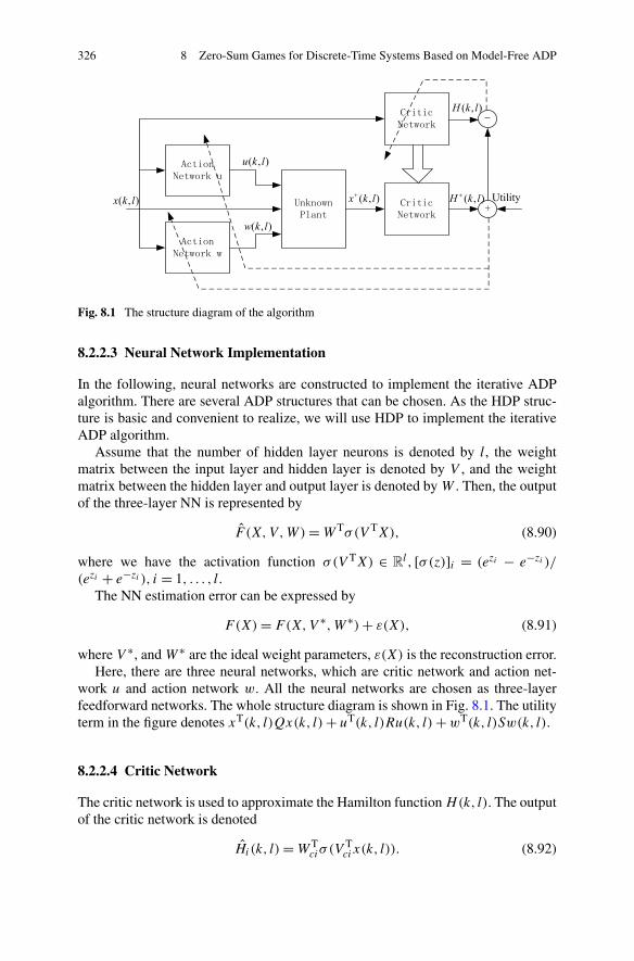
326 8 Zero-Sum Games for Discrete-Time Systems Based on Model-Free ADP
Fig. 8.1 The structure diagram of the algorithm
8.2.2.3 Neural Network Implementation
In the following, neural networks are constructed to implement the iterative ADPalgorithm. There are several ADP structures that can be chosen. As the HDP struc-ture is basic and convenient to realize, we will use HDP to implement the iterativeADP algorithm.
Assume that the number of hidden layer neurons is denoted by l, the weightmatrix between the input layer and hidden layer is denoted by V , and the weightmatrix between the hidden layer and output layer is denoted by W . Then, the outputof the three-layer NN is represented by
F (X,V,W)=WTσ(V TX), (8.90)
where we have the activation function σ(V TX) ∈ Rl , [σ(z)]i = (ezi − e−zi )/
(ezi + e−zi ), i = 1, . . . , l.The NN estimation error can be expressed by
F(X)= F(X,V ∗,W ∗)+ ε(X), (8.91)
where V ∗, and W ∗ are the ideal weight parameters, ε(X) is the reconstruction error.Here, there are three neural networks, which are critic network and action net-
work u and action network w. All the neural networks are chosen as three-layerfeedforward networks. The whole structure diagram is shown in Fig. 8.1. The utilityterm in the figure denotes xT(k, l)Qx(k, l)+ uT(k, l)Ru(k, l)+wT(k, l)Sw(k, l).
8.2.2.4 Critic Network
The critic network is used to approximate the Hamilton function H(k, l). The outputof the critic network is denoted
Hi(k, l)=WTciσ (V
Tcix(k, l)). (8.92)
8.2 Zero-Sum Differential Games for a Class of Discrete-Time 2-D Systems 327
The target function can be written as
Hi+1(k, l)= [xT(k, l) uT
i (k, l) wTi (k, l)
]⎡
⎣Q 0 00 R 00 0 S
⎤
⎦
⎡
⎣x(k, l)
ui(k, l)
wi(k, l)
⎤
⎦+H+i (k, l).
(8.93)
Then, we define the error function for the critic network as
eci(k, l)= Hi+1(k, l)−Hi+1(k, l). (8.94)
The objective function to be minimized in the critic network is
Eci(k, l)= 1
2eTci(k, l)eci(k, l). (8.95)
Therefore, the gradient-based weight updating rule for the critic network is givenby
wc(i+1)(k, l)=wci(k, l)+Δwci(k, l), (8.96)
Δwci(k, l)= αc
[−∂Eci(k, l)
∂wci(k, l)
], (8.97)
∂Eci(k, l)
∂wci(k, l)= ∂Eci(k, l)
∂Hi(k, l)
∂Hi(k, l)
∂wci(k, l), (8.98)
where αc > 0 is the learning rate of critic network and wc(k, l) is the weight vectorin the critic network.
8.2.2.5 Action Networks
Action networks are used to approximate the iterative optimal controls. There aretwo action networks, which are used to approximate the optimal control u and w,respectively.
For the action network that approximates the control u(k, l), the state x(k, l) isused as input to create the optimal control u(k, l). The output can be formulated as
ui (k, l)=WTaiσ (V
Taix(k, l)). (8.99)
Therefore, we define the output error of the action network as
eai(k, l)= ui (k, l)− ui(k, l), (8.100)
where ui(k, l) is the target function, which can be described by
ui(k, l)= (H [i]ww −H [i]
wu(H[i]uu )
−1H [i]uw)
−1
× (H [i]wu(H
[i]uu )
−1H [i]ux −H [i]
wx)x(k, l), (8.101)
where Hi can be obtained according to the Kronecker product in (8.85).
328 8 Zero-Sum Games for Discrete-Time Systems Based on Model-Free ADP
The weights of the action network are updated to minimize the following perfor-mance error measure:
Eai(k, l)= 1
2eTaieai . (8.102)
The weight updating algorithm is similar to the one for the critic network. By thegradient descent rule, we obtain
wa(i+1)(k, l)=wai(k, l)+Δwai(k, l), (8.103)
Δwai(k, l)= βa
[−∂Eai(k, l)
∂wai(k, l)
], (8.104)
∂Eai(k, l)
∂wai(k, l)= ∂Eai(k, l)
∂eai(k, l)
∂eai(k, l)
∂ui(k, l)
∂ui(k, l)
∂wai(k, l), (8.105)
where βa > 0 is the learning rate of the action network.For the action network w, the state x(k, l) is used as input to create the optimal
control w(k, l). The target of the action network w can be expressed as
wi(k, l)= (H [i]ww −H [i]
wu(H[i]uu )
−1H [i]uw)
−1
× (H [i]wu(H
[i]uu )
−1H [i]ux −H [i]
wx)x(k, l). (8.106)
All the update rules of action network w are the same as the update rules of actionnetwork u, and they are omitted here.
8.2.3 Simulations
In this subsection, the present method is applied to an air drying process control.
Example 8.12 The dynamical processes can be described by the following Darbouxequation:
∂2x(s, t)
∂s∂t= a1
∂x(s, t)
∂t+ a2
∂x(s, t)
∂x+ a0x(s, t)+ bu(s, t)+ cw(s, t), (8.107)
with the initial and boundary conditions
xh(0, t)={
0.5 t ≤ 4,
0 t > 4,and xv(s,0)=
{1 s ≤ 4,
0 s > 4,(8.108)
where x(s, t) is an unknown function, a0, a1, a2, b, and c are real coefficients, andu(s, t) and w(s, t) are the input functions. The variable x is for the humidity whichis the system state, s is for the location of the air, and t is the processing time.
8.2 Zero-Sum Differential Games for a Class of Discrete-Time 2-D Systems 329
Let a0 = 0.2, a1 = 0.3, a2 = 0.1, b = 0.3, and c = 0.25. The quadratic cost func-tional is formulated as
J =∫ ∞
t=0
∫ ∞
s=0
{xT(s, t)Qx(s, t)+ uT(s, t)Ru(s, t)
+wT(s, t)Sw(s, t)}
dtdx. (8.109)
The discretization method for the system (8.107) is similar to the method in [14].Suppose that the sampling periods of the digital control system are chosen as X =0.1cm and T = 0.1s. Following the methodology presented in [14], we compute thediscretized system equation as
[xh((k + 1)X, lT )xv(kX, (l + 1)T )
]=[
0.7408 0.27650.0952 0.9048
][xh(kX, lT )
xv(kX, lT )
]
+[
0.02590
]u(kX, lT )+
[0
0.0564
]w(kX, lT ), (8.110)
with the boundary conditions
xh(0, lT )={
0.5 l ≤ 40,
0 l > 40,and xv(kX,0)=
{1 k ≤ 40,
0 k > 40,(8.111)
and the discredited cost functional
J (x(0,0), u,w)=∞∑
k=0
∞∑
l=0
{xT(Xk,T l)Qx(Xk,T l)
+ uT(Xk,T l)Ru(Xk,T l)
+wT(Xk,T l)Sw(Xk,T l)}. (8.112)
We implement the iterative algorithm at (k, l) = (0,0). We choose three-layerneural networks as the critic network, the action network u, and the action networkw with the structure 2–8–1, 2–8–1 and 2–8–1, respectively. The initial weights ofaction networks and critic network are all set to be random in [−0.5,0.5]. Then,the critic network and the action networks are trained for i = 50 times so that thegiven accuracy ε = 10−6 is reached. In the training process, the learning rate is βa =αc = 0.05. The evaluating point number is set as N = 40 for every iteration. Choosethe small white noise as ξ1(0,0.01), ξ2(0,0.01). The convergence trajectory of thevalue function is shown in Fig. 8.2. Then, we apply the optimal control to the systemfor k = 40, l = 40 time steps and obtain the following results. The state trajectoriesare given as Figs. 8.3 and 8.4. The control trajectories are given as Figs. 8.5 and 8.6,respectively.
From the simulation results, we see that the present iterative ADP algorithm ob-tains good effects. In [14], Tsai just studied the model-based optimal control in case
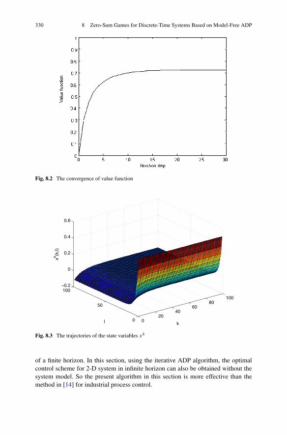
330 8 Zero-Sum Games for Discrete-Time Systems Based on Model-Free ADP
Fig. 8.2 The convergence of value function
Fig. 8.3 The trajectories of the state variables xh
of a finite horizon. In this section, using the iterative ADP algorithm, the optimalcontrol scheme for 2-D system in infinite horizon can also be obtained without thesystem model. So the present algorithm in this section is more effective than themethod in [14] for industrial process control.

8.3 Zero-Sum Games for a Class of Discrete-Time Systems via Model-Free ADP 331
Fig. 8.4 The trajectories of the state variables xv
Fig. 8.5 The trajectories of the optimal control u
8.3 Zero-Sum Games for a Class of Discrete-Time Systemsvia Model-Free ADP
A novel model-free ADP method using output feedback is developed for zero-sumgames of a class of discrete-time systems in this section. It is worthy to note thatnot only the model of the exact system is not required, but neither is the information
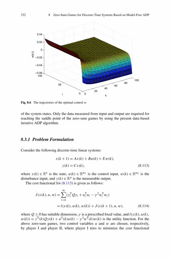
332 8 Zero-Sum Games for Discrete-Time Systems Based on Model-Free ADP
Fig. 8.6 The trajectories of the optimal control w
of the system states. Only the data measured from input and output are required forreaching the saddle point of the zero-sum games by using the present data-basediterative ADP algorithm.
8.3.1 Problem Formulation
Consider the following discrete-time linear systems:
x(k + 1)=Ax(k)+Bu(k)+Ew(k),
y(k)= Cx(k), (8.113)
where x(k) ∈ Rn is the state, u(k) ∈ R
m1 is the control input, w(k) ∈ Rm2 is the
disturbance input, and y(k) ∈Rp is the measurable output.
The cost functional for (8.113) is given as follows:
J (x(k), u,w)=∞∑
i=k
(yTi Qyi + uT
i ui − γ 2wTi wi)
= l(x(k), u(k),w(k))+ J (x(k + 1), u,w), (8.114)
where Q≥ 0 has suitable dimension, γ is a prescribed fixed value, and l(x(k), u(k),w(k)) = yT(k)Qy(k) + uT(k)u(k) − γ 2wT(k)w(k) is the utility function. For theabove zero-sum games, two control variables u and w are chosen, respectively,by player I and player II, where player I tries to minimize the cost functional
8.3 Zero-Sum Games for a Class of Discrete-Time Systems via Model-Free ADP 333
V (x(k), u,w), while player II tries to maximize it. The following assumptions areneeded; these are in effect in the remaining sections.
Assumption 8.13 The system (8.113) is controllable and observable under the con-trol variables u and w.
Assumption 8.14 The order of the system and an upper bound on its “observableindex” are known.
Assumption 8.15 There exists a unique saddle point of the zero-sum games for thesystem (8.113).
According to Assumption 8.15 and using the dynamic programming principle,the optimal value function can be expressed as
J ∗(x(k))= minu
maxw
(l(x(k), u(k),w(k))+ J ∗(x(k + 1), u,w))
= maxw
minu(l(x(k), u(k),w(k))+ J ∗(x(k + 1), u,w)). (8.115)
Because the system (8.113) is linear, there exists a matrix P that satisfies
J ∗(x(k))= xT(k)Px(k), (8.116)
where P ≥ 0 is the solution of following generalized algebraic Riccati equation(GARE):
P =ATPA+CTQC − [ATPB ATPE]
×[I +BTPB BTPE
ETPB ETPE − γ 2I
]−1 [BTPA
ETPA
]. (8.117)
The optimal control u∗(k) and w∗(k) can be derived as
u∗(k)= −(I +BTPB −BTPE(ETPE − γ 2I )−1ETPB)−1
× (BTPA−BTPE(ETPE − γ 2I )−1ETPA)x(k), (8.118)
w∗(k)= −(ETPE − γ 2I −ETPB(I +BTPB)−1BTPE)−1
× (ETPA−ETPB(I +BTPB)−1BTPA)x(k). (8.119)
For obtaining the unique feedback saddle point in the strictly feedback stabilizingcontrol policy class, the following inequalities should be satisfied [7]:
I +BTT PB > 0, (8.120)
ETPE − γ 2I > 0. (8.121)
334 8 Zero-Sum Games for Discrete-Time Systems Based on Model-Free ADP
From (8.117)–(8.119), we see that the system model is needed not only forsolving the GARE equation, but also for computing the optimal controls u∗(k)and w∗(k). To circumvent this requirement, [5] proposed the optimal strategies fordiscrete-time linear system quadratic zero-sum games without knowing the systemdynamical matrices by using the Q-learning method under the assumption that allthe states of the plant are available for feedback. Next, we propose a novel data-based optimal output feedback control scheme via the ADP algorithm, in whichneither the system model nor the system states are needed.
8.3.2 Data-Based Optimal Output Feedback Control via ADPAlgorithm
Inspired by the works in [1], according to Assumptions 8.13 and 8.14, the dynamicscan be rewritten on a time horizon [k −N,k] as the expanded state equation
x(k)=ANx(k −N)+UNuk−1,k−N + FNwk−1,k−N, (8.122)
yk−1,k−N = VNx(k −N)+ TN uk−1,k−N +GNwk−1,k−N, (8.123)
where
uk−1,k−N = [u(k − 1) u(k − 2) . . . u(k −N) ]T ∈Rm1N,
wk−1,k−N = [w(k − 1) w(k − 2) . . . w(k −N) ]T ∈Rm2N,
yk−1,k−N = [y(k − 1) y(k − 2) . . . y(k −N)
]T ∈ RpN,
VN =[CAN−1 . . . CA C
]T,
UN =[B AB A2B . . . AN−1B
],
FN =[E AE A2E . . . AN−1E
],
TN =
⎡
⎢⎢⎢⎢⎢⎣
0 CB CAB . . . CAN−2B
0 0 CB . . . CAN−3B...
.... . .
. . ....
0 . . . . . . 0 CB
0 0 0 0 0
⎤
⎥⎥⎥⎥⎥⎦,
GN =
⎡
⎢⎢⎢⎢⎢⎣
0 CE CAE . . . CAN−2E
0 0 CE . . . CAN−3E...
.... . .
. . ....
0 . . . . . . 0 CE
0 0 0 0 0
⎤
⎥⎥⎥⎥⎥⎦. (8.124)
8.3 Zero-Sum Games for a Class of Discrete-Time Systems via Model-Free ADP 335
Since the system (8.113) is observable under the control variables u and w, thereexists a upper bound on the observability index K , such that rank(VN) < n forN < K and rank(VN) = n for N > K . Choose N > K ; we have rank(VN) = n.Then, there exists a matrix M ∈ R
n×pN such that
AN =MVN. (8.125)
Since rank(VN)= n, its left inverse is given as
V +N = (V T
NVN)−1V T
N. (8.126)
Then M can be rearranged as the sum of two parts,
M =ANV +N +Z(I − VNV
+N )≡M0 +M1, (8.127)
for any matrix Z, with M0 denoting the minimum norm operator and P(R⊥)(VN)=I − VNV
+N being the projection onto a range perpendicular to VN .
Theorem 8.16 (cf. [10]) Using Assumption 8.14, the system state x(k) is givenuniquely in terms of the measured input–output data sequences yk−1,k−N , uk−1,k−N ,and wk−1,k−N by
x(k)=M0yk−1,k−N + (UN −M0TN)uk−1,k−N
+ (FN −M0GN)wk−1,k−N
=Myyk−1,k−N +Muuk−1,k−N +Mwwk−1,k−N, (8.128)
where My =M0, Mu =UN −M0TN , and Mw = FN −M0GN .
Proof Multiplying x(k −N) by both sides of (8.123), and using (8.125), we have
ANx(k −N)=MVNx(k −N)
=Myk−1,k−N −MTNuk−1,k−N −MGNwk−1,k−N. (8.129)
Then, using (8.127), we have
(M0 +M1)VNx(k −N)= (M0 +M1)yk−1,k−N − (M0 +M1)TN uk−1,k−N
− (M0 +M1)GNwk−1,k−N . (8.130)
Since M1VN = 0, we have
MVNx(k −N)=M0VNx(k −N). (8.131)
Multiplying both sides of (8.123), we have
0 =M1yk−1,k−N −M1TN uk−1,k−N −M1GNwk−1,k−N
∀M1 s.t. M1VN = 0. (8.132)
336 8 Zero-Sum Games for Discrete-Time Systems Based on Model-Free ADP
Then, using (8.129)–(8.132), we have
ANx(k −N)=M0VNx(k −N)
=M0yk−1,k−N −M0TN uk−1,k−N −M0GNwk−1,k−N . (8.133)
From (8.122), it follows that
x(k)=M0yk−1,k−N + (UN −M0TN)uk−1,k−N
+ (FN −M0GN)wk−1,k−N
=Myyk−1,k−N +Muuk−1,k−N +Mwwk−1,k−N. (8.134)
This completes the proof. �
Remark 8.17 From (8.134), we see that the state variable is completely eliminatedfrom the right-hand side of (8.113). That is, x(k) can be reconstructed by the avail-able measured input–output data sequence yk−1,k−N , uk−1,k−N , and wk−1,k−N .
Next, we will derive the optimal controls u∗ and w∗ by using the available mea-surable input–output data.
Define
zk−1,k−N =⎡
⎣uk−1,k−N
wk−1,k−N
yk−1,k−N
⎤
⎦ . (8.135)
We have
V (x(k), u,w)= x(k)TPx(k)
= zTk−1,k−N
⎡
⎢⎣MT
u
MTw
MTy
⎤
⎥⎦P [Mu Mw My]zk−1,k−N
= zTk−1,k−N
⎡
⎢⎣MT
u PMu MTu PMw MT
u PMy
MTwPMu M
TwPMw MT
wPMy
MTy PMu M
Ty PMw MT
y PMy
⎤
⎥⎦ zk−1,k−N
= zTk−1,k−NP zk−1,k−N, (8.136)
where z ∈R(m1+m2+p)N and P ∈R
(m1+m2+p)N×(m1+m2+p)N .By rewriting (8.115) and using (8.134), we have
(u∗(k),w∗(k))= arg minu
maxw
{yT(k)Qy(k)+ uT(k)u(k)− γ 2wT(k)w(k)
+ zTk,k−N+1P zk,k−N+1
}. (8.137)
8.3 Zero-Sum Games for a Class of Discrete-Time Systems via Model-Free ADP 337
Partition zTk,k−N+1P zk,k−N+1 as
zTk,k−N+1P zk,k−N+1
=
⎡
⎢⎢⎢⎢⎣
u(k)
uk−1,k−N+1w(k)
wk−1,k−N+1yk,k−N+1
⎤
⎥⎥⎥⎥⎦
T⎡
⎢⎢⎢⎢⎣
Puu Puu Puw Puw PuyPuu Puu Puw Puw PuyPwu Pwu Pww Pww PwyPwu Pwu Pww Pww PwyPyu Pyu Pyw Pyw Pyy
⎤
⎥⎥⎥⎥⎦
⎡
⎢⎢⎢⎢⎣
u(k)
uk−1,k−N+1w(k)
wk−1,k−N+1yk,k−N+1
⎤
⎥⎥⎥⎥⎦. (8.138)
Then differentiating with respect to u(k) to perform the minimization in (8.137)yields
u(k)= −(I + Puu)−1(Puuuk−1,k−N+1 + Puww(k)
+ Puwwk−1,k−N+1 + Puy yk,k−N+1). (8.139)
Similarly, differentiating with respect to w(k) to perform the maximization in(8.137) yields
w(k)= −(Pww − γ 2I )(Pwuu(k)+ Pwuuk−1,k−N+1
+ Pwwwk−1,k−N+1 + Pwyyk,k−N+1). (8.140)
Thus, substitute (8.140) into (8.139), and u∗(k) can be derived as
u∗(k)= −(I + Puu − Puw(Pww − γ 2I )Pwu)−1[−Puw(Pww − γ 2I )−1
× (Pwuuk−1,k−N+1 + Pwwwk−1,k−N+1 + Pwyyk,k−N+1)
+ Puuuk−1,k−N+1 + Puwwk−1,k−N+1 + Puy yk,k−N+1]. (8.141)
Similarly, substitute (8.139) into (8.140), and w∗(k) can be derived as
w∗(k)= −(Pww − γ 2I − Pwu(I + Puu)−1Puw)
−1[−Pwu(R + Puu)−1
× (Puuuk−1,k−N+1 + Puwwk−1,k−N+1 + Puy yk,k−N+1)
+ Pwuuk−1,k−N+1 + Pwwwk−1,k−N+1 + Pwy yk,k−N+1]. (8.142)
Comparing (8.118)–(8.119) with (8.141)–(8.142), it is important to note that theoptimal control u∗ and w∗ expressed by (8.141)–(8.142) can be obtained if P can besolved. Neither knowledge of the system dynamics A, B , E, and C, nor informationof the measurable state x(k) is needed.
In the following, the uniqueness of the optimal control is discussed.
Theorem 8.18 (cf. [10]) The optimal controls generated by (8.141) and (8.142)are independent of M1 and depend only on M0. Moreover, (8.141) and (8.142) areequivalent to
338 8 Zero-Sum Games for Discrete-Time Systems Based on Model-Free ADP
u∗(k)= −(I +BTPB −BTPE(ETPE − γ 2I )−1ETPB)−1
× [− Puw(Pww − γ 2I )−1
× (Pwuuk−1,k−N+1 + Pwwwk−1,k−N+1 + Pwyyk,k−N+1)
+ Puuuk−1,k−N+1 + Puwwk−1,k−N+1 + Puy yk,k−N+1], (8.143)
w∗(k)= −[ETPE − γ 2I −ETPB(I +BTPB)−1BTPE]−1
× [− Pwu(I + Puu)−1
× (Puuuk−1,k−N+1 + Puwwk−1,k−N+1 + Puy yk,k−N+1)
+ Pwuuk−1,k−N+1 + Pwwwk−1,k−N+1 + Pwyyk,k−N+1], (8.144)
where Pwu, Pww , Pwy , Puu, Puw , and Puy depend only on M0.
Proof Rewrite (8.139) as
0 = u(k)+ Puuu(k)+ Puuuk−1,k−N+1 + Puww(k)
+ Puwwk−1,k−N+1 + Puy yk,k−N+1
= u(k)+ [Puu Puu |Puw Puw |Puy]⎡
⎣uk,k−N+1wk,k−N+1yk,k−N+1
⎤
⎦ . (8.145)
According to (8.136) and (8.138), we have
[Puu Puu] = [Im1 0]MTu PMu,
[Puw Puw] = [Im1 0]MTu PMw,
Puy = [Im1 0]MTu PMy. (8.146)
After substituting (8.146) into (8.145), we have
0 = u(k)+ [Puu Puu |Puw Puw |Puy]⎡
⎣uk,k−N+1wk,k−N+1yk,k−N+1
⎤
⎦
= u(k)+ [Im1 0]MTu P
× [Muuk,k−N+1 +Mwwk,k−N+1 +Myyk,k−N+1]= u(k)+ [Im1 0]MT
u P
× [M0yk−1,k−N + (UN −M0TN)uk−1,k−N
+ (FN −M0GN)wk−1,k−N ]. (8.147)
8.3 Zero-Sum Games for a Class of Discrete-Time Systems via Model-Free ADP 339
According to Theorem 8.16, (8.147) is unique and independent of M1. Using thestructure of UN , TN , FN , and GN , it follows that
Mu
[Im1
0
]= (UN −M0TN)
[Im1
0
]= B, (8.148)
Mw
[Im2
0
]= (FN −M0GN)
[Im2
0
]=E. (8.149)
Then,
Puu = [Im1 0]MTu PMu
[Im1
0
]= BTPB, (8.150)
Puw = [Im1 0]MTu PMw
[Im2
0
]= BTPE, (8.151)
Pwu = [Im2 0]MTwPMu
[Im1
0
]=ETPB. (8.152)
Substituting (8.150)–(8.152) to (8.139), we obtain
u(k)= −(I +BTPB)−1(Puuuk−1,k−N+1 +BTPEw(k)
+ Puwwk−1,k−N+1 + Puy yk,k−N+1). (8.153)
Similarly, we obtain
w(k)= −(ETPE − γ 2I )(ETPBu(k)+ Pwuuk−1,k−N+1
+ Pwwwk−1,k−N+1 + Pwy yk,k−N+1). (8.154)
Then, substituting (8.154) into (8.153), we have (8.143). By a similar method,(8.144) can also be obtained.
This completes the proof. �
Although we have obtained the optimal control expressed in (8.141)–(8.142) withthe information of the matrix P , it is not straightforward to solve P in most cases.Therefore, next we propose the data-based iterative ADP algorithm for zero-sumgames of (8.113).
First, the initial value of P is set as P0 = 0, which is not necessarily optimal.Then, for i = 0,1, . . . , the matrix Pi associated with the cost function
Vi(x(k), u,w) and control policy ui(k) and wi(k) can be updated by implementingthe iteration between
zTk−1,k−NPi+1zk−1,k−N = yT(k)Qy(k)+ uT
i (k)ui(k)− γ 2wTi (k)wi(k)
+ zTk,k−NPi zk,k−N, (8.155)
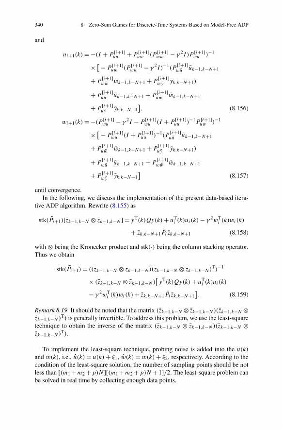
340 8 Zero-Sum Games for Discrete-Time Systems Based on Model-Free ADP
and
ui+1(k)= −(I + P [i+1]uu + P [i+1]
uw (P [i+1]ww − γ 2I )P [i+1]
wu )−1
× [− P [i+1]uw (P [i+1]
ww − γ 2I )−1(P[i+1]wu uk−1,k−N+1
+ P[i+1]ww wk−1,k−N+1 + P
[i+1]wy yk,k−N+1)
+ P[i+1]uu uk−1,k−N+1 + P
[i+1]uw wk−1,k−N+1
+ P[i+1]uy yk,k−N+1
], (8.156)
wi+1(k)= −(P [i+1]wu − γ 2I − P [i+1]
wu (I + P [i+1]uu )−1P [i+1]
uw )−1
× [− P [i+1]wu (I + P [i+1]
uu )−1(P[i+1]uu uk−1,k−N+1
+ P[i+1]uw wk−1,k−N+1 + P
[i+1]uy yk,k−N+1)
+ P[i+1]wu uk−1,k−N+1 + P
[i+1]ww wk−1,k−N+1
+ P[i+1]wy yk,k−N+1
](8.157)
until convergence.In the following, we discuss the implementation of the present data-based itera-
tive ADP algorithm. Rewrite (8.155) as
stk(Pi+1)[zk−1,k−N ⊗ zk−1,k−N ] = yT(k)Qy(k)+ uTi (k)ui(k)− γ 2wT
i (k)wi(k)
+ zk,k−N+1Pi zk,k−N+1 (8.158)
with ⊗ being the Kronecker product and stk(·) being the column stacking operator.Thus we obtain
stk(Pi+1)= ((zk−1,k−N ⊗ zk−1,k−N)(zk−1,k−N ⊗ zk−1,k−N)T)−1
× (zk−1,k−N ⊗ zk−1,k−N)[yT(k)Qy(k)+ uT
i (k)ui(k)
− γ 2wTi (k)wi(k)+ zk,k−N+1Pi zk,k−N+1
]. (8.159)
Remark 8.19 It should be noted that the matrix (zk−1,k−N ⊗ zk−1,k−N)(zk−1,k−N ⊗zk−1,k−N)
T) is generally invertible. To address this problem, we use the least-squaretechnique to obtain the inverse of the matrix (zk−1,k−N ⊗ zk−1,k−N)(zk−1,k−N ⊗zk−1,k−N)
T).
To implement the least-square technique, probing noise is added into the u(k)
and w(k), i.e., u(k)= u(k)+ ξ1, w(k)= w(k)+ ξ2, respectively. According to thecondition of the least-square solution, the number of sampling points should be notless than [(m1 +m2 +p)N ][(m1 +m2 +p)N +1]/2. The least-square problem canbe solved in real time by collecting enough data points.
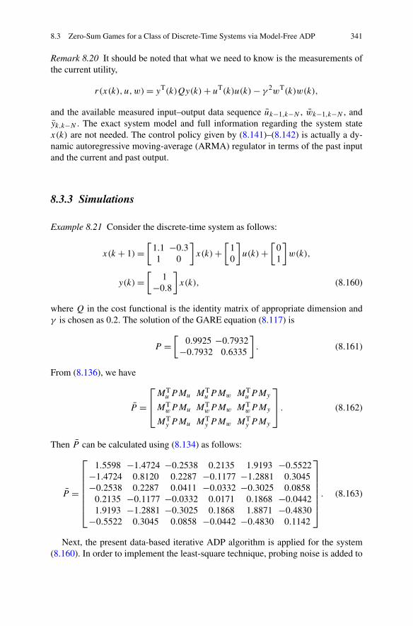
8.3 Zero-Sum Games for a Class of Discrete-Time Systems via Model-Free ADP 341
Remark 8.20 It should be noted that what we need to know is the measurements ofthe current utility,
r(x(k), u,w)= yT(k)Qy(k)+ uT(k)u(k)− γ 2wT(k)w(k),
and the available measured input–output data sequence uk−1,k−N , wk−1,k−N , andyk,k−N . The exact system model and full information regarding the system statex(k) are not needed. The control policy given by (8.141)–(8.142) is actually a dy-namic autoregressive moving-average (ARMA) regulator in terms of the past inputand the current and past output.
8.3.3 Simulations
Example 8.21 Consider the discrete-time system as follows:
x(k + 1)=[
1.1 −0.31 0
]x(k)+
[10
]u(k)+
[01
]w(k),
y(k)=[
1−0.8
]x(k), (8.160)
where Q in the cost functional is the identity matrix of appropriate dimension andγ is chosen as 0.2. The solution of the GARE equation (8.117) is
P =[
0.9925 −0.7932−0.7932 0.6335
]. (8.161)
From (8.136), we have
P =⎡
⎢⎣MT
u PMu MTu PMw MT
u PMy
MTwPMu MT
wPMw MTwPMy
MTy PMu MT
y PMw MTy PMy
⎤
⎥⎦ . (8.162)
Then P can be calculated using (8.134) as follows:
P =
⎡
⎢⎢⎢⎢⎢⎢⎣
1.5598 −1.4724 −0.2538 0.2135 1.9193 −0.5522−1.4724 0.8120 0.2287 −0.1177 −1.2881 0.3045−0.2538 0.2287 0.0411 −0.0332 −0.3025 0.0858
0.2135 −0.1177 −0.0332 0.0171 0.1868 −0.04421.9193 −1.2881 −0.3025 0.1868 1.8871 −0.4830
−0.5522 0.3045 0.0858 −0.0442 −0.4830 0.1142
⎤
⎥⎥⎥⎥⎥⎥⎦. (8.163)
Next, the present data-based iterative ADP algorithm is applied for the system(8.160). In order to implement the least-square technique, probing noise is added to
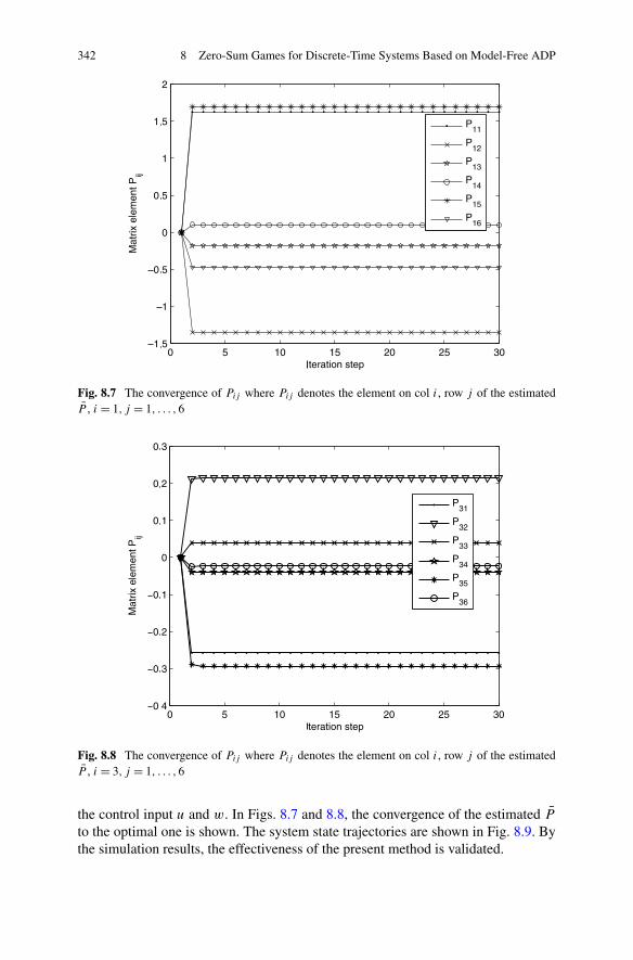
342 8 Zero-Sum Games for Discrete-Time Systems Based on Model-Free ADP
Fig. 8.7 The convergence of Pij where Pij denotes the element on col i, row j of the estimatedP , i = 1, j = 1, . . . ,6
Fig. 8.8 The convergence of Pij where Pij denotes the element on col i, row j of the estimatedP , i = 3, j = 1, . . . ,6
the control input u and w. In Figs. 8.7 and 8.8, the convergence of the estimated P
to the optimal one is shown. The system state trajectories are shown in Fig. 8.9. Bythe simulation results, the effectiveness of the present method is validated.
8.4 Summary 343
Fig. 8.9 The trajectories of system states
8.4 Summary
We studied the zero-sum games for discrete-time systems based on the model-freeADP method in this chapter. In Sect. 8.2, an effective data-based optimal controlscheme was developed via the iterative ADP algorithm to find the optimal con-troller of a class of discrete-time zero-sum games for Roesser type 2-D systems.The present method allows implementation without the system model. In Sect. 8.2,a data-based optimal output feedback controller was developed for solving the zero-sum games of a class of discrete-time systems, whose merit is that not only knowl-edge of system model is not required, but also information of the system states isnot. The theoretical analysis and simulation study showed the validity of the presentmethods.
References
1. Aangenent W, Kostic D, de Jager B, Van de Molengraft R, Steinbuch M (2005) Data-basedoptimal control. In: Proceedings of American control conference, Portland, pp 1460–1465
2. Abu-Khalaf M, Lewis FL (2008) Neurodynamic programming and zero-sum games for con-strained control systems. IEEE Trans Neural Netw 19:1243–1252
3. Abu-Khalaf M, Lewis FL, Huang J (2006) Policy iterations on the Hamilton–Jacobi–Isaacsequation for H∞ state feedback control with input saturation. IEEE Trans Autom Control51:1989–1995
4. Al-Tamimi A, Abu-Khalaf M, Lewis FL (2007) Adaptive critic designs for discrete-time zero-sum games with application to H∞ control. IEEE Trans Syst Man Cybern, Part B, Cybern37:240–247
344 8 Zero-Sum Games for Discrete-Time Systems Based on Model-Free ADP
5. Al-Tamimi A, Lewis FL, Abu-Khalaf M (2007) Model-free q-learning designs for lineardiscrete-time zero-sum games with application to H∞ control. Automatica 43:473–481
6. Al-Tamimi A, Lewis FL, Abu-Khalaf M (2007) Model-free Q-learning designs for lineardiscrete-time zero-sum games with application to H-infinity control. Automatica 43:473–481
7. Basar T, Bernhard P (1995) H∞ optimal control and related minimax design problems.Birkhauser, Basel
8. Basar T, Olsder GJ (1982) Dynamic noncooperative game theory. Academic Press, New York9. Bertsekas DP (2003) Convex analysis and optimization. Athena Scientific, Boston
10. Cui LL, Zhang HG, Zhang X, Luo YH (2011) Adaptive critic design based output feedbackcontrol for discrete-time zero-sum games. In: Proceedings of IEEE symposium on adaptivedynamic programming and reinforcement learning, France, pp 190–195
11. Hua X, Mizukami K (1994) Linear-quadratic zero-sum differential games for generalized statespace systems. IEEE Trans Autom Control 39:143–147
12. Li CJ, Fadali MS (1991) Optimal control of 2-D systems. IEEE Trans Autom Control 36:223–228
13. Luenberger DG (1969) Optimization by vector space methods. Wiley, New York14. Tsai JS, Li JS, Shieh LS (2002) Discretized quadratic optimal control for continuous-time
two-dimensional systems. IEEE Trans Circuits Syst I, Fundam Theory Appl 49:116–12515. Uetake Y (1992) Optimal smoothing for noncausal 2-D systems based on a descriptor model.
IEEE Trans Autom Control 37:1840–184516. Wei QL, Zhang HG, Cui LL (2009) Data-based optimal control for discrete-time zero-sum
games of 2-D systems using adaptive critic designs. Acta Autom Sin 35:682–692
Chapter 9Nonlinear Games for a Classof Continuous-Time Systems Based on ADP
9.1 Introduction
Game theory is concerned with the study of decision making in situations wheretwo or more rational opponents are involved under conditions of conflicting inter-ests. This has been widely investigated by many authors [5, 7, 8, 12, 13]. Thoughthe nonlinear optimal solution in term of Hamilton–Jacobi–Bellman equation ishard to obtain directly [4], it is still fortunate that there is only one controller ordecision maker. In the previous chapter, we have studied discrete-time zero-sumgames based on the ADP method. In this chapter, we will consider continuous-timegames.
For zero-sum differential games, the existence of the saddle point is proposedbefore obtaining the saddle point in much of the literature [1, 6, 11]. In many realworld applications, however, the saddle point of a game may not exist, which meansthat we can only obtain the mixed optimal solution of the game. In Sect. 9.2, we willstudy how to obtain the saddle point without complex existence conditions of thesaddle point and how to obtain the mixed optimal solution when the saddle pointdoes not exist based on the ADP method for a class of affine nonlinear zero-sumgames. Note that many applications of practical zero-sum games have nonaffinecontrol input. In Sect. 9.3, we will focus on finite horizon zero-sum games for aclass of nonaffine nonlinear systems.
The non-zero-sum differential games theory also has a number of potential ap-plications in control engineering, economics and the military field [9]. For zero-sumdifferential games, two players work on a cost functional together and minimax it.However, for non-zero-sum games, the control objective is to find a set of policiesthat guarantee the stability of the system and minimize the individual performancefunction to yield a Nash equilibrium. In Sect. 9.4, non-zero-sum differential gameswill be studied using a single network ADP.
H. Zhang et al., Adaptive Dynamic Programming for Control,Communications and Control Engineering, DOI 10.1007/978-1-4471-4757-2_9,© Springer-Verlag London 2013
345
346 9 Nonlinear Games for a Class of Continuous-Time Systems Based on ADP
9.2 Infinite Horizon Zero-Sum Games for a Class of AffineNonlinear Systems
In this section, the nonlinear infinite horizon zero-sum differential games is studied.We propose a new iterative ADP method which is effective for both the situationthat the saddle point does and does not exist. For the situation that the saddle pointexists, the existence conditions of the saddle point are avoided. The value functioncan reach the saddle point using the present iterative ADP method. For the situationthat the saddle point does not exist, the mixed optimal value function is obtainedunder a deterministic mixed optimal control scheme, using the present iterative ADPalgorithm.
9.2.1 Problem Formulation
Consider the following two-person zero-sum differential games. The system is de-scribed by the continuous-time affine nonlinear equation
x(t)= f (x(t), u(t),w(t))= f (x(t))+ g(x(t))u(t)+ k(x(t))w(t), (9.1)
where x(t) ∈Rn, u(t) ∈R
k , w(t) ∈ Rm, and the initial condition x(0)= x0 is given.
The cost functional is the generalized quadratic form given by
J (x(0), u,w)=∫ ∞
0l(x, u,w)dt, (9.2)
where l(x, u,w) = xTAx + uTBu + wTCw + 2uTDw + 2xTEu + 2xTFw. Thematrices A, B , C, D, E, and F have suitable dimensions and A ≥ 0, B > 0,and C < 0. According to the situation of two players we have the followingdefinitions. Let J (x) := infu supw J (x,u,w) be the upper value function andJ (x) := supw infu J (x,u,w) be the lower value function with the obvious inequal-ity J (x) ≥ J (x). Define the optimal control pairs to be (u,w) and (u,w) for up-per and lower value functions, respectively. Then, we have J (x) = J (x,u,w) andJ (x)= J (x,u,w).
If both J (x) and J (x) exist and
J (x)= J (x)= J ∗(x) (9.3)
holds, we say that the saddle point exists and the corresponding optimal control pairis denoted by (u∗,w∗).
We have the following lemma.
Lemma 9.1 If the nonlinear system (9.1) is controllable and both the upper valuefunction and lower value function exist, then J (x) is a solution of the following
9.2 Infinite Horizon Zero-Sum Games for a Class of Affine Nonlinear Systems 347
upper Hamilton–Jacobi–Isaacs (HJI) equation:
infu
supw
{J t + JTxf (x,u,w)+ l(x, u,w)} = 0, (9.4)
which is denoted by HJI(J (x),u,w) = 0 and J (x) is a solution of the followinglower HJI equation:
supw
infu
{J t + J Txf (x,u,w)+ l(x, u,w)} = 0, (9.5)
which is denoted by HJI(J (x),u,w)= 0.
9.2.2 Zero-Sum Differential Games Based on Iterative ADPAlgorithm
As the HJI equations (9.4) and (9.5) cannot be solved in general, in the following,a new iterative ADP method for zero-sum differential games is developed.
9.2.2.1 Derivation of the Iterative ADP Method
The goal of the present iterative ADP method is to obtain the saddle point. As thesaddle point may not exist, this motivates us to obtain the mixed optimal valuefunction J o(x) where J (x)≤ J o(x)≤ J (x).
Theorem 9.2 (cf. [15]) Let (u,w) be the optimal control pair for J (x) and (u,w)
be the optimal control pair for J (x). Then, there exist control pairs (u,w) and(u,w) which lead to J o(x) = J (x,u,w) = J (x,u,w). Furthermore, if the saddlepoint exists, then J o(x)= J ∗(x).
Proof According to the definition of J (x), we have J (x,u,w) ≤ J (x,u,w). AsJ o(x) is a mixed optimal value function, we also have J o(x) ≤ J (x,u,w). Asthe system (9.1) is controllable and w is continuous on R
m, there exists a con-trol pair (u,w) which makes J o(x) = J (x,u,w). On the other hand, we haveJ o(x) ≥ J (x,u,w). We also have J (x,u,w) ≥ J (x,u,w). As u is continuouson R
k , there exists a control pair (u,w) which makes J o(x) = J (x,u,w). If thesaddle point exists, we have (9.3). On the other hand, J (x)≤ J o(x)≤ J (x). Then,clearly J o(x)= J ∗(x). �
If (9.3) holds, we have a saddle point; if not, we adopt a mixed trajectory to obtainthe mixed optimal solution of the game. To apply the mixed trajectory method, thegame matrix is necessary under the trajectory sets of the control pair (u,w). SmallGaussian noises γu ∈ Rk and γw ∈ Rm are introduced that are added to the optimal
348 9 Nonlinear Games for a Class of Continuous-Time Systems Based on ADP
control u and w, respectively, where γ iu(0, σ2i ), i = 1, . . . , k, and γ
jw(0, σ 2
j ), j =1, . . . ,m, are zero-mean Gaussian noises with variances σ 2
i and σ 2j , respectively.
We define the expected value function asE(J (x)) = minPIi maxPIIj
∑2i=1
∑2j=1 PIiLijPIIj , where we let L11 =
J (x,u,w), L12 = J (x, (u + γu),w), L21 = J (x,u,w) and L22 = J (x,u,
(w + γw)). Let∑2
i=1 PIi = 1 and PIi > 0. Let∑2
j=1 PIIj = 1 and PIIj > 0. Next,let N be a large enough positive integer. Calculating the expected value function N
times, we can obtain E1(J (x)),E2(J (x)), . . . ,EN(J (x)). Then, the mixed optimalvalue function can be written as
J o(x)=E(Ei(J (x)))= 1
N
N∑
i=1
Ei(J (x)).
Remark 9.3 In the classical mixed trajectory method, the whole control sets Rk
and Rm should be searched under some distribution functions. As there are no con-
straints for both controls, we see that there exist controls that cause the system to beunstable. This is not permitted for real-world control systems. Thus, it is impossibleto search the whole control sets and we can only search the local area around thestable controls which guarantees stability of the system. This is the reason why thesmall Gaussian noises γu and γw are introduced. So the meaning of the Gaussiannoises can be seen in terms of the local stable area of the control pairs. A proposi-tion will be given to show that the control pair chosen in the local area is stable (seeProposition 9.14). Similar work can also be found in [3, 14].
We can see that the mixed optimal solution is a mathematically expectedvalue which means that it cannot be obtained in reality once the trajectoriesare determined. For most practical optimal control problems, however, the ex-pected optimal solution (or mixed optimal solution) has to be achieved. Toovercome this difficulty, a new method is developed in this section. Let α =(J o(x)− J (x))/(J (x)− J (x)). Then, J o(x) can be written as J o(x) = αJ (x) +(1 − α)J (x). Let lo(x,u,w,u,w) = αl(x,u,w) + (1 − α)l(x,u,w). We haveJ o(x(0)) = ∫∞
0 lodt . According to Theorem 9.2, the mixed optimal control paircan be obtained by regulating the control w in the control pair (u,w) that mini-mizes the error between J (x) and J o(x) where the value function J (x) is definedas J (x(0))= J (x(0), u,w)= ∫∞
0 l(x, u,w)dt and J (x(0))≤ J (x(0))≤ J (x(0)).Define J (x(0))= ∫∞
0 l(x,w)dx, where l(x,w)= l(x, u,w)− lo(x,u,w,u,w).Then, the problem can be described as minw(J (x))2.
According to the principle of optimality, when J (x) ≥ 0 we have the followingHJB equation:
HJB(J (x),w) := minw
{Jt (x)+ Jxf (x,u,w)+ l(x,w)} = 0. (9.6)
For J (x) < 0, we have −J (x) = −(J (x)− J o(x)) > 0, and we can obtain thesame HJB equation as (9.6).
9.2 Infinite Horizon Zero-Sum Games for a Class of Affine Nonlinear Systems 349
9.2.2.2 The Iterative ADP Algorithm
Given the above preparation, we now formulate the iterative ADP algorithm forzero-sum differential games as follows:
1. Initialize the algorithm with a stabilizing control pair (u[0],w[0]), and the valuefunction is V [0]. Choose the computation precision ζ > 0. Set i = 0.
2. For the upper value function, let
V[i](x(0))=
∫ ∞
0l(x, u[i+1],w[i+1])dt, (9.7)
where the iterative optimal control pair is formulated as
u[i+1] = − 1
2(B −DC−1DT)−1(2(kT −DC−1F T)x
+ (gT(x)−DC−1kT(x))V[i]x
), (9.8)
and
w[i+1] = −1
2C−1(2DTu[i+1] + 2F Tx + kT(x)V
[i]x
). (9.9)
(u[i],w[i]) satisfies the HJI equation HJI(V[i](x), u[i],w[i]) = 0, and V
[i]x =
dV[i](x)/dx.
3. If |V [i+1](x(0))− V
[i](x(0))|< ζ , let u= u[i], w =w[i] and J (x)= V
[i+1](x).
Set i = 0 and go to Step 4. Else, set i = i + 1 and go to Step 2.4. For the lower value function, let
V [i](x(0))=∫ ∞
0l(x, u[i+1],w[i+1])dt, (9.10)
where the iterative optimal control pair is formulated as
u[i+1] = −1
2g−1(2Dw[i+1] + 2kTx + gT(x)V [i]
x ), (9.11)
and
w[i+1] = − 1
2(C −DTBD)−1(2(F T −DTg−1E)x
+ (kT(x)−DTg−1gT(x))V [i]x ). (9.12)
(u[i],w[i]) satisfies the HJI equation HJI(V [i](x), u[i],w[i]) = 0, and V [i]x =
dV [i](x)/dx.5. If |V [i+1](x(0))− V [i](x(0))|< ζ , let u= u[i], w =w[i] and J (x)= V [i+1](x).
Set i = 0 and go to Step 6. Else, set i = i + 1 and go to Step 4.6. If |J (x(0))− J (x(0))|< ζ , stop, and the saddle point is achieved. Else set i = 0
and go to the next step.
350 9 Nonlinear Games for a Class of Continuous-Time Systems Based on ADP
7. Regulate the control w for the upper value function and let
J [i+1](x(0))= V [i+1](x(0))− J o(x(0)) (9.13)
=∫ ∞
0l(x, u,w[i])dt.
The iterative optimal control is formulated as
w[i] = −1
2C−1(2DTu+ 2F Tx + kT(x)V [i+1]
x ), (9.14)
where V [i]x = dV [i](x)/dx.
8. If |V [i+1](x(0))− J o(x(0))|< ζ , stop. Else, set i = i + 1 and go to Step 7.
9.2.2.3 Properties of the Iterative ADP Algorithm
In this part, some results are presented to show the stability and convergence of thepresent iterative ADP algorithm.
Theorem 9.4 (cf. [15]) If for ∀i ≥ 0, HJI(V[i](x), u[i],w[i])= 0 holds, and for ∀t ,
l(x,u[i],w[i]) ≥ 0, then the control pairs (u[i],w[i]) make system (9.1) asymptoti-cally stable.
Proof According to (9.7), for ∀ t , taking the derivative of V[i](x), we have
dV[i](x)
dt= V
[i]Tx
(f (x)+ g(x)u[i+1] + k(x)w[i+1]) . (9.15)
From the HJI equation we have
0 = V[i]Tx f (x,u[i],w[i])+ l(x, u[i],w[i]). (9.16)
Combining (9.15) and (9.16), we get
dV[i](x)
dt=V
[i]Tx (g(x)− k(x)C−1DT)(u[i+1] − u[i])
− xTAx − u[i]T(B −DC−1DT)u[i] − 1
4V
[i]Tx k(x)C−1kT(x)V
[i]x
− 2xT(E − FC−1DT)u[i+1] + xTFC−1F Tx. (9.17)
According to (9.8) we have
dV[i](x)
dt= − (u[i+1] − u[i])T(B −DC−1DT)
9.2 Infinite Horizon Zero-Sum Games for a Class of Affine Nonlinear Systems 351
× (u[i+1] − u[i])− l(x, u[i+1],w(i+1))
≤0. (9.18)
So, V[i](x) is a Lyapunov function. Let ε > 0 and ‖x(t0)‖< δ(ε). Then, there exist
two functions α(‖x‖) and β(‖x‖) which belong to class K and satisfy
α(ε)≥ β(δ)≥ V[i](x(t0))≥ V
[i](x(t))≥ α(‖x‖). (9.19)
Therefore, system (9.1) is asymptotically stable. �
Theorem 9.5 (cf. [15]) If for ∀ i ≥ 0, HJI(V [i](x), u[i],w[i])= 0 holds, and for ∀ t ,l(x, u[i],w[i]) < 0, then the control pairs (u[i],w[i]) make system (9.1) asymptoti-cally stable.
Corollary 9.6 If for ∀i ≥ 0, HJI(V [i](x), u[i],w[i]) = 0 holds, and for ∀t ,l(x, u[i],w[i]) ≥ 0, then the control pairs (u[i],w[i]) make system (9.1) asymptoti-cally stable.
Proof As V [i](x)≤ V[i](x) and l(x, u[i],w[i])≥ 0, we have 0 ≤ V [i](x)≤ V
[i](x).
From Theorem 9.4, we know that for ∀t0, there exist two functions α(‖x‖) andβ(‖x‖) which belong to class K and satisfy (9.19).
As V[i](x)→ 0, there exist time instants t1 and t2 (without loss of generality, let
t0 < t1 < t2) that satisfy
V[i](x(t0))≥ V
[i](x(t1))≥ V [i](x(t0))≥ V
[i](x(t2)). (9.20)
Choose ε1 > 0 that satisfies V [i](x(t0)) ≥ α(ε1) ≥ V[i](x(t2)). Then, there exists
δ1(ε1) > 0 that makes α(ε1)≥ β(δ1)≥ V[i](x(t2)). Then, we obtain
V [i](x(t0))≥ α(ε1)≥ β(δ1)≥ V[i](x(t2))≥ V
[i](x(t))≥ V [i](x(t))≥ α(‖x‖).
(9.21)
According to (9.19), we have
α(ε)≥ β(δ)≥ V [i](x(t0))≥ α(ε1)≥ β(δ1)≥ V [i](x(t))≥ α(‖x‖). (9.22)
Since α(‖x‖) belongs to class K, we obtain ‖x‖ ≤ ε.Therefore, we conclude that the system (9.1) is asymptotically stable. �
Corollary 9.7 If for ∀i ≥ 0, HJI(V[i](x), u[i],w[i]) = 0 holds, and for ∀t ,
l(x,u[i],w[i]) < 0, then the control pairs (u[i],w[i]) make system (9.1) asymptoti-cally stable.
352 9 Nonlinear Games for a Class of Continuous-Time Systems Based on ADP
Theorem 9.8 (cf. [15]) If for ∀i ≥ 0, HJI(V[i](x), u[i],w[i]) = 0 holds, and
l(x,u[i],w[i]) is the utility function, then the control pairs (u[i],w[i]) make system(9.1) asymptotically stable.
Proof For the time sequence t0 < t1 < t2 < · · · < tm < tm+1 < · · · , without loss ofgenerality, we assume l(x, u[i],w[i]) ≥ 0 in [t2n, t(2n+1)) and l(x, u[i],w[i]) < 0 in[t2n+1, t(2(n+1))) where n= 0,1, . . . .
Then, for t ∈ [t0, t1) we have l(x, u[i],w[i]) ≥ 0 and∫ t1t0l(x, u[i],w[i])dt ≥ 0.
According to Theorem 9.4, we have ‖x(t0)‖ ≥ ‖x(t)‖ ≥ ‖x(t1)‖.For t ∈ [t1, t2) we have l(x, u[i],w[i]) < 0 and
∫ t2t1l(x, u[i],w[i])dt < 0. Accord-
ing to Corollary 9.7, we have ‖x(t1)‖ > ‖x(t)‖ > ‖x(t2)‖. So we obtain ‖x(t0)‖ ≥‖x(t)‖> ‖x(t2)‖, for ∀t ∈ [t0, t2).
Using mathematical induction, for ∀t , we have ‖x(t ′)‖ ≤ ‖x(t)‖ where t ′ ∈[t,∞). So we conclude that the system (9.1) is asymptotically stable, and the proofis completed. �
Theorem 9.9 (cf. [15]) If for ∀i ≥ 0, HJI(V [i](x), u[i],w[i]) = 0 holds, and
l(x, u[i],w[i]) is the utility function, then the control pairs (u[i],w[i]) make system(9.1) asymptotically stable.
Next, we will give the convergence proof of the iterative ADP algorithm.
Proposition 9.10 If for ∀i ≥ 0, HJI(V[i](x), u[i],w[i]) = 0 holds, then the control
pairs (u[i],w[i]) make the upper value function V[i](x)→ J (x) as i → ∞.
Proof According to HJI (V[i](x), u[i],w[i]) = 0, we obtain dV
[i+1](x)/dt by re-
placing the index “i” by the index “i + 1”:
dV[i+1]
(x)
dt= −(xTAx + u(i+1)T(B −DC−1DT)u[i+1]
+ 1
4V
[i]Tx k(x)C−1kT(x)V
[i]x + 2xT(E − FC−1DT)u[i+1]
− xTFC−1F Tx). (9.23)
According to (9.18), we obtain
d(V[i+1]
(x)− V[i](x))
dt= dV
[i+1](x)
dt− dV
[i](x)
dt
= (u[i+1] − u[i])T(B −DC−1DT(u[i+1] − u[i])
> 0. (9.24)
Since the system (9.1) is asymptotically stable, its state trajectories x converge
to zero, and so does V[i+1]
(x) − V[i](x). Since d(V
[i+1](x)− V
[i](x))/dt ≥ 0
9.2 Infinite Horizon Zero-Sum Games for a Class of Affine Nonlinear Systems 353
on these trajectories, it implies that V[i+1]
(x) − V[i](x) ≤ 0; that is V
[i+1](x) ≤
V[i](x). Thus, V
[i](x) is convergent as i → ∞.
Next, we define limi→∞ V[i](x)= V
[∞](x).
For ∀i, let w∗ = arg maxw{∫ ttl(x, u,w)dτ + V
[i](x(t))}. Then, according to the
principle of optimality, we have
V[i](x)≤ sup
w
{∫ t
t
l(x, u,w)dτ + V[i](x(t))
}
=∫ t
t
l(x, u,w∗)dτ + V[i](x(t)). (9.25)
Since V[i+1]
(x)≤ V[i](x), we have V
[∞](x)≤ ∫ t
tl(x, u,w∗)dτ + V
[i](x(t)).
Letting i → ∞, we obtain V[∞]
(x) ≤ ∫ ttl(x, u,w∗)dτ + V
[∞](x(t)). So, we
have V[∞]
(x)≤ infu supw{∫ ttl(x, u,w)dt + V
[i](x(t))}.
Let ε > 0 be an arbitrary positive number. Since the upper value function is non-
increasing and convergent, there exists a positive integer i such that V[i](x)− ε ≤
V[∞]
(x)≤ V[i](x).
Let u∗ = arg minu{∫ ttl(x, u,w∗)dτ + V
[i](x(t))}. Then we get V
[i](x) =
∫ ttl(x, u∗,w∗)dτ + V
[i](x(t)).
Thus, we have
V[∞]
(x)≥∫ t
t
l(x, u∗,w∗)dτ + V[i](x(t))− ε
≥∫ t
t
l(x, u∗,w∗)dτ + V[∞]
(x(t))− ε (9.26)
= infu
supw
{∫ t
t
l(x, u,w)dτ + V[∞]
(x(t))
}− ε.
Since ε is arbitrary, we have
V[∞]
(x)≥ infu
supw
{∫ t
t
l(x, u,w)dτ + V[∞]
(x(t))
}.
Therefore, we obtain
V[∞]
(x)= infu
supw
{∫ t
t
l(x, u,w)dτ + V[∞]
(x(t))
}.
Let t → ∞, we have
V[∞]
(x)= infu
supw
J (x,u,w)= J (x). �
354 9 Nonlinear Games for a Class of Continuous-Time Systems Based on ADP
Proposition 9.11 If for ∀i ≥ 0, HJI(V [i](x), u[i],w[i]) = 0 holds, then the controlpairs (u[i],w[i]) make the lower value function V [i](x)→ J (x) as i → ∞.
Theorem 9.12 (cf. [15]) If the saddle point of the zero-sum differential game ex-
ists, then the control pairs (u[i],w[i]) and (u[i],w[i]) make V[i](x) → J ∗(x) and
V [i](x)→ J ∗(x), respectively, as i → ∞.
Proof For the upper value function, according to Proposition 9.10, we have
V[i](x)→ J (x) under the control pairs (u[i],w[i]) as i → ∞. So the optimal control
pair for the upper value function satisfies J (x)= J (x,u,w)= infu supw J (x,u,w).On the other hand, there exists an optimal control pair (u∗,w∗) making the value
reach the saddle point. According to the property of the saddle point, the optimalcontrol pair (u∗,w∗) satisfies J ∗(x)= J (x,u∗,w∗)= infu supw J (x,u,w).
So, we have V[i](x) → J ∗(x) under the control pair (u[i],w[i]) as i → ∞.
Similarly, we can derive V [i](x) → J ∗(x) under the control pairs (u[i],w[i]) asi → ∞. �
Remark 9.13 From the proofs we see that the complex existence conditions of thesaddle point in [1, 2] are not necessary. If the saddle point exists, the iterative valuefunctions can converge to the saddle point using the present iterative ADP algorithm.
In the following part, we emphasize that when the saddle point does not exist,the mixed optimal solution can be obtained effectively using the iterative ADP al-gorithm.
Proposition 9.14 If u ∈ Rk , w[i] ∈ R
m and the utility function is l(x,w[i]) =l(x,u,w[i]) − lo(x,u,w,u,w), and w[i] is expressed in (9.14), then the controlpairs (u,w[i]) make the system (9.1) asymptotically stable.
Proposition 9.15 If u ∈ Rk , w[i] ∈ R
m and for ∀t , the utility function l(x,w[i])≥ 0,then the control pairs (u,w[i]) make V [i](x) a nonincreasing convergent sequenceas i → ∞.
Proposition 9.16 If u ∈ Rk , w[i] ∈ R
m and for ∀t , the utility function l(x,w[i]) < 0,then the control pairs (u,w[i]) make V [i](x) a nondecreasing convergent sequenceas i → ∞.
Theorem 9.17 (cf. [15]) If u ∈ Rk , w[i] ∈ R
m, and l(x,w[i]) is the utility function,then the control pairs (u,w[i]) make V [i](x) convergent as i → ∞.
Proof For the time sequence t0 < t1 < t2 < · · · < tm < tm+1 < · · · , withoutloss of generality, we suppose l(x,w[i]) ≥ 0 in [t2n, t2n+1) and l(x,w[i]) < 0 in[t2n+1, t2(n+1)), where n= 0,1, . . . .
9.2 Infinite Horizon Zero-Sum Games for a Class of Affine Nonlinear Systems 355
For t ∈ [t2n, t2n+1) we have l(x,w[i]) ≥ 0 and∫ t1t0l(x,w[i])dt ≥ 0. Accord-
ing to Proposition 9.15, we have V [i+1](x) ≤ V [i](x). For t ∈ [t2n+1, t2(n+1)) wehave l(x,w[i]) < 0 and
∫ t2t1l(x,w[i])dt < 0. According to Proposition 9.16 we have
V [i+1](x) > V [i](x). Then, for ∀t0, we have
∥∥∥V [i+1](x(t0))∥∥∥=
∥∥∥∥∫ t1
t0
l(x,w[i])dt∥∥∥∥+
∥∥∥∥∫ t2
t1
l(x,w[i])dt∥∥∥∥
+ . . .+∥∥∥∥∫ t(m+1)
tm
l(x,w[i])dt∥∥∥∥+ . . .
<
∥∥∥V [i](x(t0))∥∥∥ . (9.27)
So, V [i](x) is convergent as i → ∞. �
Theorem 9.18 (cf. [15]) If u ∈ Rk , w[i] ∈ Rm, and l(x,w[i]) is the utility function,then the control pairs (u,w[i]) make V [i](x)→ J o(x) as i → ∞.
Proof It is proved by contradiction. Suppose that the control pair (u,w[i]) makesthe value function V [i](x) converge to J ′(x) and J ′(x) �= J o(x).
According to Theorem 9.17, based on the principle of optimality, as i → ∞ wehave the HJB equation HJB(J (x),w)= 0.
From the assumptions we know that |V [i](x)−J o(x)| �= 0 as i → ∞. From The-orem 9.5, we know that there exists a control pair (u,w′) that makes J (x,u,w′)=J o(x), which minimizes the performance index function J (x). According to theprinciple of optimality, we also have the HJB equation HJB(J (x),w′)= 0.
It is a contradiction. So the assumption does not hold. Thus, we have V [i](x)→J o(x) as i → ∞. �
Remark 9.19 For the situation where the saddle point does not exist, the methodsin [1, 2] are all invalid. Using our iterative ADP method, the iterative value functionreaches the mixed optimal value function J o(x) under the deterministic control pair.Therefore, we emphasize that the present iterative ADP method is more effective.
9.2.3 Simulations
Example 9.20 The dynamics of the benchmark nonlinear plant can be expressed bysystem (9.1) where
f (x)=[x2
−x1+εx24 sinx3
1 − ε2cos2x3x4
ε cosx3(x1−εx24 sinx3)
1 − ε2cos2x3
]T
,
g(x)=[
0−ε cosx3
1 − ε2cos2x30
1
1 − ε2cos2x3
]T
,
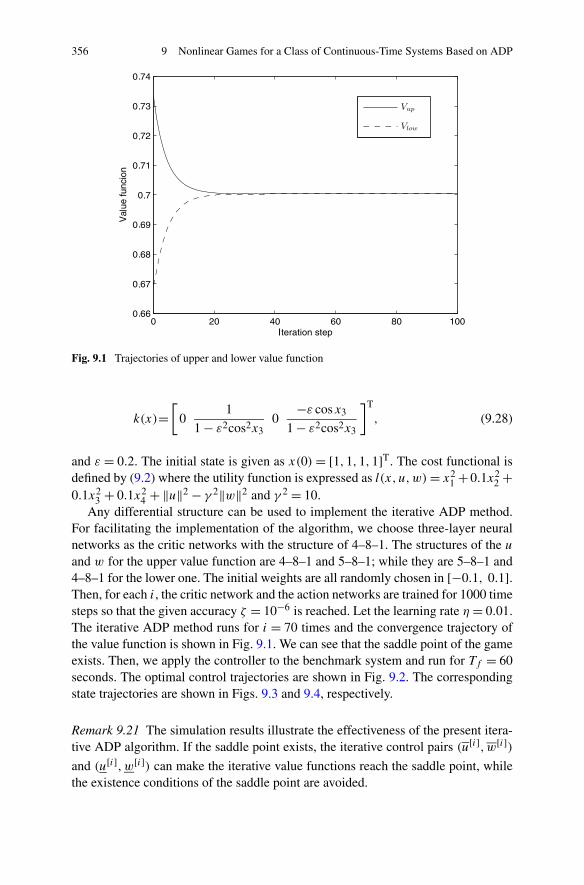
356 9 Nonlinear Games for a Class of Continuous-Time Systems Based on ADP
Fig. 9.1 Trajectories of upper and lower value function
k(x)=[
01
1 − ε2cos2x30
−ε cosx3
1 − ε2cos2x3
]T
, (9.28)
and ε = 0.2. The initial state is given as x(0) = [1,1,1,1]T. The cost functional isdefined by (9.2) where the utility function is expressed as l(x, u,w)= x2
1 + 0.1x22 +
0.1x23 + 0.1x2
4 + ‖u‖2 − γ 2‖w‖2 and γ 2 = 10.Any differential structure can be used to implement the iterative ADP method.
For facilitating the implementation of the algorithm, we choose three-layer neuralnetworks as the critic networks with the structure of 4–8–1. The structures of the uand w for the upper value function are 4–8–1 and 5–8–1; while they are 5–8–1 and4–8–1 for the lower one. The initial weights are all randomly chosen in [−0.1, 0.1].Then, for each i, the critic network and the action networks are trained for 1000 timesteps so that the given accuracy ζ = 10−6 is reached. Let the learning rate η = 0.01.The iterative ADP method runs for i = 70 times and the convergence trajectory ofthe value function is shown in Fig. 9.1. We can see that the saddle point of the gameexists. Then, we apply the controller to the benchmark system and run for Tf = 60seconds. The optimal control trajectories are shown in Fig. 9.2. The correspondingstate trajectories are shown in Figs. 9.3 and 9.4, respectively.
Remark 9.21 The simulation results illustrate the effectiveness of the present itera-tive ADP algorithm. If the saddle point exists, the iterative control pairs (u[i],w[i])and (u[i],w[i]) can make the iterative value functions reach the saddle point, whilethe existence conditions of the saddle point are avoided.
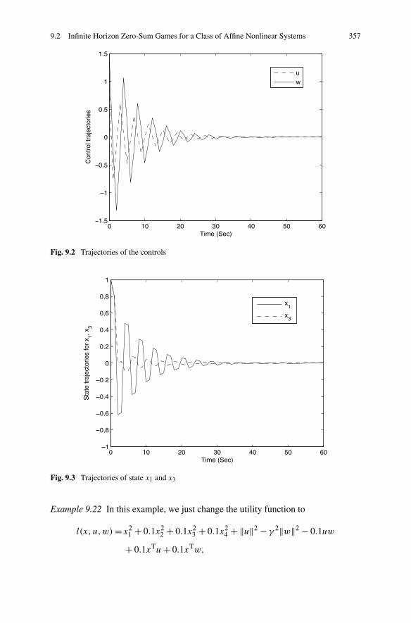
9.2 Infinite Horizon Zero-Sum Games for a Class of Affine Nonlinear Systems 357
Fig. 9.2 Trajectories of the controls
Fig. 9.3 Trajectories of state x1 and x3
Example 9.22 In this example, we just change the utility function to
l(x, u,w)=x21 + 0.1x2
2 + 0.1x23 + 0.1x2
4 + ‖u‖2 − γ 2‖w‖2 − 0.1uw
+ 0.1xTu+ 0.1xTw,
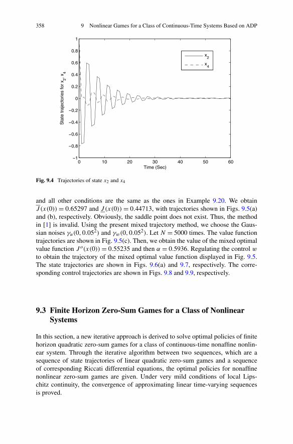
358 9 Nonlinear Games for a Class of Continuous-Time Systems Based on ADP
Fig. 9.4 Trajectories of state x2 and x4
and all other conditions are the same as the ones in Example 9.20. We obtainJ (x(0)) = 0.65297 and J (x(0)) = 0.44713, with trajectories shown in Figs. 9.5(a)and (b), respectively. Obviously, the saddle point does not exist. Thus, the methodin [1] is invalid. Using the present mixed trajectory method, we choose the Gaus-sian noises γu(0,0.052) and γw(0,0.052). Let N = 5000 times. The value functiontrajectories are shown in Fig. 9.5(c). Then, we obtain the value of the mixed optimalvalue function J o(x(0))= 0.55235 and then α = 0.5936. Regulating the control wto obtain the trajectory of the mixed optimal value function displayed in Fig. 9.5.The state trajectories are shown in Figs. 9.6(a) and 9.7, respectively. The corre-sponding control trajectories are shown in Figs. 9.8 and 9.9, respectively.
9.3 Finite Horizon Zero-Sum Games for a Class of NonlinearSystems
In this section, a new iterative approach is derived to solve optimal policies of finitehorizon quadratic zero-sum games for a class of continuous-time nonaffine nonlin-ear system. Through the iterative algorithm between two sequences, which are asequence of state trajectories of linear quadratic zero-sum games and a sequenceof corresponding Riccati differential equations, the optimal policies for nonaffinenonlinear zero-sum games are given. Under very mild conditions of local Lips-chitz continuity, the convergence of approximating linear time-varying sequencesis proved.
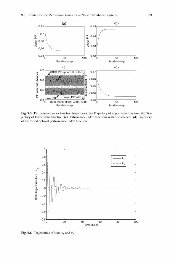
9.3 Finite Horizon Zero-Sum Games for a Class of Nonlinear Systems 359
Fig. 9.5 Performance index function trajectories. (a) Trajectory of upper value function. (b) Tra-jectory of lower value function. (c) Performance index functions with disturbances. (d) Trajectoryof the mixed optimal performance index function
Fig. 9.6 Trajectories of state x1 and x3
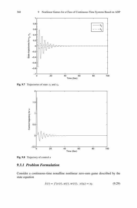
360 9 Nonlinear Games for a Class of Continuous-Time Systems Based on ADP
Fig. 9.7 Trajectories of state x2 and x4
Fig. 9.8 Trajectory of control u
9.3.1 Problem Formulation
Consider a continuous-time nonaffine nonlinear zero-sum game described by thestate equation
x(t)= f (x(t), u(t),w(t)), x(t0)= x0 (9.29)
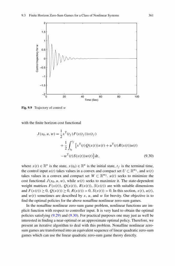
9.3 Finite Horizon Zero-Sum Games for a Class of Nonlinear Systems 361
Fig. 9.9 Trajectory of control w
with the finite horizon cost functional
J (x0, u,w)= 1
2xT(tf )F (x(tf ))x(tf )
+ 1
2
∫ tf
t0
[xT(t)Q(x(t))x(t)+ uT(t)R(x(t))u(t)
−wT(t)S(x(t))w(t)]
dt, (9.30)
where x(t) ∈ Rn is the state, x(t0) ∈ R
n is the initial state, tf is the terminal time,the control input u(t) takes values in a convex and compact set U ⊂ R
m1 , and w(t)
takes values in a convex and compact set W ⊂ Rm2 . u(t) seeks to minimize the
cost functional J (x0, u,w), while w(t) seeks to maximize it. The state-dependentweight matrices F(x(t)), Q(x(t)), R(x(t)), S(x(t)) are with suitable dimensionsand F(x(t))≥ 0, Q(x(t))≥ 0, R(x(t)) > 0, S(x(t)) > 0. In this section, x(t), u(t),and w(t) sometimes are described by x, u, and w for brevity. Our objective is tofind the optimal policies for the above nonaffine nonlinear zero-sum games.
In the nonaffine nonlinear zero-sum game problem, nonlinear functions are im-plicit function with respect to controller input. It is very hard to obtain the optimalpolicies satisfying (9.29) and (9.30). For practical purposes one may just as well beinterested in finding a near-optimal or an approximate optimal policy. Therefore, wepresent an iterative algorithm to deal with this problem. Nonaffine nonlinear zero-sum games are transformed into an equivalent sequence of linear quadratic zero-sumgames which can use the linear quadratic zero-sum game theory directly.
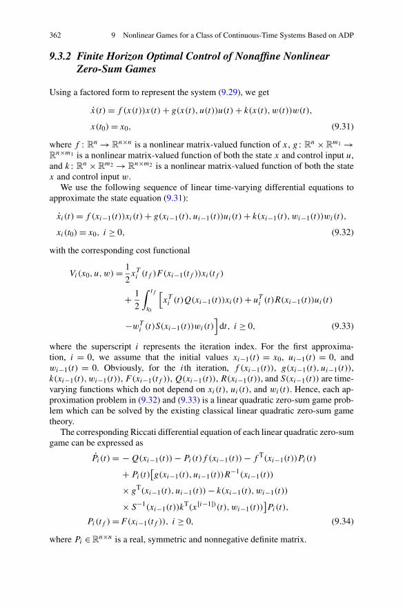
362 9 Nonlinear Games for a Class of Continuous-Time Systems Based on ADP
9.3.2 Finite Horizon Optimal Control of Nonaffine NonlinearZero-Sum Games
Using a factored form to represent the system (9.29), we get
x(t)= f (x(t))x(t)+ g(x(t), u(t))u(t)+ k(x(t),w(t))w(t),
x(t0)= x0, (9.31)
where f : Rn → Rn×n is a nonlinear matrix-valued function of x, g : Rn ×R
m1 →Rn×m1 is a nonlinear matrix-valued function of both the state x and control input u,
and k : Rn ×Rm2 → R
n×m2 is a nonlinear matrix-valued function of both the statex and control input w.
We use the following sequence of linear time-varying differential equations toapproximate the state equation (9.31):
xi (t)= f (xi−1(t))xi(t)+ g(xi−1(t), ui−1(t))ui(t)+ k(xi−1(t),wi−1(t))wi(t),
xi(t0)= x0, i ≥ 0, (9.32)
with the corresponding cost functional
Vi(x0, u,w)= 1
2xTi (tf )F (xi−1(tf ))xi(tf )
+ 1
2
∫ tf
t0
[xTi (t)Q(xi−1(t))xi(t)+ uTi (t)R(xi−1(t))ui(t)
−wTi (t)S(xi−1(t))wi(t)
]dt, i ≥ 0, (9.33)
where the superscript i represents the iteration index. For the first approxima-tion, i = 0, we assume that the initial values xi−1(t) = x0, ui−1(t) = 0, andwi−1(t) = 0. Obviously, for the ith iteration, f (xi−1(t)), g(xi−1(t), ui−1(t)),k(xi−1(t),wi−1(t)), F(xi−1(tf )), Q(xi−1(t)), R(xi−1(t)), and S(xi−1(t)) are time-varying functions which do not depend on xi(t), ui(t), and wi(t). Hence, each ap-proximation problem in (9.32) and (9.33) is a linear quadratic zero-sum game prob-lem which can be solved by the existing classical linear quadratic zero-sum gametheory.
The corresponding Riccati differential equation of each linear quadratic zero-sumgame can be expressed as
Pi(t)= −Q(xi−1(t))− Pi(t)f (xi−1(t))− f T(xi−1(t))Pi(t)
+ Pi(t)[g(xi−1(t), ui−1(t))R
−1(xi−1(t))
× gT(xi−1(t), ui−1(t))− k(xi−1(t),wi−1(t))
× S−1(xi−1(t))kT(x[i−1])(t),wi−1(t))
]Pi(t),
Pi(tf )=F(xi−1(tf )), i ≥ 0, (9.34)
where Pi ∈Rn×n is a real, symmetric and nonnegative definite matrix.
9.3 Finite Horizon Zero-Sum Games for a Class of Nonlinear Systems 363
Assumption 9.23 It is assumed that S(xi−1(t)) > S i , where the threshold valueS i is defined as S i = inf{Si(t) > 0, and (9.34) does not have a conjugate point on[0, tf ]}.
If Assumption 9.23 is satisfied, the game admits the optimal policies given by
ui(t)= −R−1(xi−1(t))gT(xi−1(t), ui−1(t))Pi(t)xi(t),
wi(t)= S−1(xi−1(t))kT(xi−1(t),wi−1(t))Pi(t)xi(t), i ≥ 0, (9.35)
where xi(t) is the corresponding optimal state trajectory, generated by
xi (t)=[f (xi−1(t))− g(xi−1(t), ui−1(t))R−1(xi−1(t))
× gT(xi−1(t), ui−1(t))Pi(t)+ k(xi−1(t),wi−1(t))
× S−1(xi−1(t))kT(xi−1(t),wi−1(t))Pi(t)
]xi(t),
xi(t0)=x0. (9.36)
By using the iteration between sequences (9.34) and (9.36) sequently, the limitof the solution of the approximating sequence (9.32) will converge to the unique so-lution of system (9.29), and the sequences of optimal policies (9.35) will converge,too. The convergence of iterative algorithm will be analyzed in the next section. No-tice that the factored form in (9.31) does not need to be unique. The approximatinglinear time-varying sequences will converge whatever the representation of f (x(t)),g(x(t), u(t)), and k(x(t),w(t)).
Remark 9.24 For the fixed finite interval [t0, tf ], if S(xi−1(t)) > S i , the Riccati dif-ferential equation (9.34) has a conjugate point on [t0, tf ]. It means that Vi(x0, u,w)
is strictly concave in w. Otherwise, since Vi(x0, u,w) is quadratic and R(t) > 0,F(t) ≥ 0, Q(t) ≥ 0, it follows that Vi(x0, u,w) is strictly convex in u. Hence, forlinear quadratic zero-sum games (9.32) with the performance index function (9.34)there exists a unique saddle point; they are the optimal policies.
The convergence of the algorithm described above requires the following:
1. The sequence {xi(t)} converges on C([t0, tf ];Rn), which means that the limit ofthe solution of approximating sequence (9.32) converges to the unique solutionof system (9.29).
2. The sequences of optimal policies {ui(t)} and {wi(t)} converge on C([t0, tf ];Rm1) and C([t0, tf ];Rm2), respectively.
For simplicity, the approximating sequence (9.32) is rewritten as
xi (t)= f (xi−1(t))xi(t)+G(xi−1(t), ui−1(t))xi(t)+K(xi−1(t),wi−1(t))xi(t),
xi(t0)= x0, i ≥ 0, (9.37)
364 9 Nonlinear Games for a Class of Continuous-Time Systems Based on ADP
where
G(xi−1, ui−1)Δ= − g(xi−1(t), ui−1(t))R
−1(xi−1(t))T(xi−1(t), ui−1(t))Pi(t),
K(xi−1,wi−1)Δ= k(xi−1(t),wi−1(t))S
−1(xi−1(t))kT(xi−1(t),wi−1(t))Pi(t).
The optimal policies for zero-sum games are rewritten as
ui(t)=M(xi−1(t), ui−1(t))xi(t),
wi(t)=N(xi−1(t),wi−1(t))xi(t), (9.38)
where
M(xi−1, ui−1)Δ= −R−1(xi−1(t))g
T(xi−1(t), ui−1(t))Pi(t),
N(xi−1,wi−1)Δ= S−1(xi−1(t))k
T(xi−1(t),wi−1(t))Pi(t).
Assumption 9.25 g(x,u), k(x,w), R−1(x), S−1(x), F(x) and Q(x) are boundedand Lipschitz continuous in their arguments x, u, and w, thus satisfying:
(C1) ‖g(x,u)‖ ≤ b, ‖k(x,u)‖ ≤ e
(C2) ‖R−1(x)‖ ≤ r , ‖S−1(x)‖ ≤ s
(C3) ‖F(x)‖ ≤ f , ‖Q(x)‖ ≤ q
for ∀x ∈ Rn, ∀u ∈ R
m1 , ∀w ∈ Rm2 , and for finite positive numbers b, e, r , s, f ,
and q .
Define Φi−1(t, t0) as the transition matrix generated by fi−1(t). It is well knownthat
‖Φi−1(t, t0)‖ ≤ exp
[∫ t
t0
μ(f (xi−1(τ )))dτ
], t ≥ t0, (9.39)
where μ(f ) is the measure of matrix f , μ(f ) = limh→0+ ‖I+hf ‖−1h
. We use thefollowing lemma to get an estimate for Φi−1(t, t0)−Φi−2(t, t0).
The following lemma is relevant for the solution of the Riccati differential equa-tion (9.34), which is the basis for proving the convergence.
Lemma 9.26 Let Assumption 9.25 hold; the solution of the Riccati differentialequation (9.34) satisfies:
1. Pi(t) is Lipschitz continuous.2. Pi(t) is bounded, if the linear time-varying system (9.32) is controllable.
Proof First, let us prove that Pi(t) is Lipschitz continuous. We transform (9.34) intothe form of a matrix differential equation:
[λi (t)
Xi(t)
]=[−f (xi−1(t)) −Q(xi−1(t))
Ξ f (xi−1(t))
][λi(t)
Xi(t)
],
[λi(tf )
Xi(tf )
]=[F(tf )
I
],
9.3 Finite Horizon Zero-Sum Games for a Class of Nonlinear Systems 365
where
Ξ =g(xi−1(t), ui−1(t))R−1(xi−1(t))g
T(xi−1(t), ui−1(t))
− k(xi−1(t),wi−1(t))S−1(xi−1(t))k
T(xi−1(t),wi−1(t)).
Thus, the solution Pi(t) of the Riccati differential equations (9.34) becomes
Pi(t)= λi(t) (Xi(t))−1 . (9.40)
If Assumption 9.25 is satisfied, such that f (x), g(x,u), k(x,w), R−1(x), S−1(x),F(x), and Q(x) are Lipschitz continuous, then Xi(t) and λi(t) are Lipschitz con-tinuous. Furthermore, it is easy to verify that (Xi(t))
−1 also satisfies the Lipschitzcondition. Hence, Pi(t) is Lipschitz continuous.
Next, we prove that Pi(t) is bounded.If the linear time varying system (9.32) is controllable, there must exist
ui (t), wi(t) such that x(t1)= 0 at t = t1. We define ui (t), wi(t) as
ui (t)={ui (t), t ∈ [0, t1)0, t ∈ [t1,∞)
wi(t)={wi(t)= S−1(xi−1(t))k
T(xi−1(t),wi−1(t))Pi(t)xi(t), t ∈ [0, t1)0, t ∈ [t1,∞)
where ui (t) is any control policy making x(t1)= 0, wi(t) is defined as the optimalpolicy. We have t ≥ t1, and we let ui (t) and wi(t) be 0, the state x(t) will still holdat 0.
The optimal cost functional V ∗i (x0, u,w) described as
V ∗i (x0, u,w)= 1
2xTi (tf )F (xi−1(tf ))xi(tf )+ 1
2
∫ tf
t0
[xTi (t)Q(xi−1(t))xi(t)
+ u∗Ti (t)R(xi−1(t))u
∗i (t)−w∗T
i (t)S(xi−1(t))w∗i (t)
]dt, (9.41)
where u∗i (t) and w∗
i (t) are the optimal policies. V ∗i (x0, u,w) is minimized by u∗(t)
and maximized by w∗i (t).
For the linear system, V ∗i (x0, u,w) can be expressed as V ∗
i (x0, u,w) =1/(2xT
i (t)Pi(t)xi(t)). Since xi(t) is arbitrary, if V ∗i (x0, u,w) is bounded, then
Pi(t) is bounded. Next, we discuss the boundedness of V ∗i (x0, u,w) in two
cases:
Case 1: t1 < tf ; we have
V ∗i (x0, u,w)≤ 1
2xTi (tf )F (xi−1(tf ))xi(tf )+ 1
2
∫ tf
t0
[xTi (t)Q(xi−1(t))xi(t)
+ uTi (t)R(xi−1(t))ui (t)−w∗T
i (t)S(xi−1(t))w∗i (t)
]dt
366 9 Nonlinear Games for a Class of Continuous-Time Systems Based on ADP
= 1
2
∫ t1
t0
[xTi (t)Q(xi−1(t))xi(t)
+ uTi (t)R(xi−1(t))ui (t)−w∗T
i (t)S(xi−1(t))w∗i (t)
]dt
=Vt1i (x)
<∞. (9.42)
Case 2: t1 ≥ tf ; we have
V ∗i (x0, u,w)≤ 1
2xTi (tf )F (xi−1(tf ))xi(tf )+ 1
2
∫ tf
t0
[xTi (t)Q(xi−1(t))xi(t)
+ uTi (t)R(xi−1(t))ui(t)−w∗T
i (t)S(xi−1(t))w∗i (t)
]dt
≤ 1
2
∫ ∞
t0
[xTi (t)Q(xi−1(t))xi(t)
+ uTi (t)R(xi−1(t))ui(t)− wT
i (t)S(xi−1(t))wi(t)]dt
= 1
2
∫ t1
t0
[xTi (t)Q(xi−1(t))xi(t)
+ uTi (t)R(xi−1(t))ui(t)−w∗T
i (t)S(xi−1(t))w∗i (t)
]dt
=Vt1i (x)
<∞. (9.43)
From (9.42) and (9.43), we know that V ∗i (x) has an upper bound, independent of tf .
Hence, Pi(t) is bounded. �
According to Lemma 9.26, Pi(t) is bounded and Lipschitz continuous. If As-sumption 9.25 is satisfied, then M(x,u), N(x,w), G(x,w), and K(x,w) arebounded and Lipschitz continuous in their arguments, thus satisfying:
(C4) ‖M(x,u)‖ ≤ δ1, ‖N(x,w)‖ ≤ σ1,(C5) ‖M(x1, u1) − M(x2, u2)‖ ≤ δ2‖x1 − x2‖ + δ3‖u1 − u2‖, ‖N(x1,w1) −
N(x2,w2)‖ ≤ σ2‖x1 − x2‖ + σ3‖w1 −w2‖,(C6) ‖G(x,u)‖ ≤ ζ1, ‖K(x,w)‖ ≤ ξ1,(C7) ‖G(x1, u1) − G(x2, u2)‖ ≤ ζ2‖x1 − x2‖ + ζ3‖u1 − u2‖, ‖K(x1,w1) −
K(x2,w2)‖ ≤ ξ2‖x1 − x2‖ + ξ3‖w1 −w2‖,
∀x ∈ Rn, ∀u ∈ R
m1 , ∀w ∈ Rm2 , and for finite positive numbers δj , σj , ζj , ξj , j =
1,2,3.
Theorem 9.27 (cf. [16]) Consider the system (9.29) of nonaffine nonlinear zero-sum games with the cost functional (9.30), the approximating sequences (9.32) and(9.33) can be introduced. We have F(x(t))≥ 0, Q(x(t))≥ 0, R(x(t)) > 0, and theterminal time tf is specified. Let Assumption 9.25, and Assumptions (A1) and (A2)
9.3 Finite Horizon Zero-Sum Games for a Class of Nonlinear Systems 367
hold and S(x(t)) > S, for small enough tf or x0; then the limit of the solution of theapproximating sequence (9.32) converges to the unique solution of system (9.29) onC([t0, tf ];Rn). Meanwhile, the approximating sequences of optimal policies givenby (9.35) also converge on C([t0, tf ];Rm1) and C([t0, tf ];Rm2), if
‖Ψ (t)‖< 1, (9.44)
where
Ψ (t)=⎡
⎣ψ1 ψ2 ψ3ψ4 ψ5 ψ6ψ7 ψ8 ψ9
⎤
⎦ ,
ψ1(t)={[
ζ2+ξ2ζ1+ξ1
+ α(t − t0)]e(ζ1+ξ1)(t−t0) − ζ2+ξ2
ζ1+ξ1
}
(1 + ζ1+ξ1
μ0
(1 − eμ0(t−t0)
)) ‖x0‖ eμ0(t−t0),
ψ2(t)=ζ3
ζ1+ξ1‖x0‖ eμ0(t−t0)(e(ζ1+ξ1)(t−t0) − 1)(
1 + ζ1+ξ1μ0
(1 − eμ0(t−t0)
)) ,
ψ3(t)=ξ3
ζ1+ξ1‖x0‖ eμ0(t−t0)(e(ζ1+ξ1)(t−t0) − 1)(
1 + ζ1+ξ1μ0
(1 − eμ0(t−t0)
)) ,
ψ4(t)= δ1ψ1(t)+ δ2 ‖x0‖ e(μ0+ζ1+ξ1)(t−t0),
ψ5(t)= δ1ψ2(t)+ δ3 ‖x0‖ e(μ0+ζ1+ξ1)(t−t0),
ψ6(t)= δ1ψ3(t),
ψ7(t)= σ1ψ1(t)+ σ2 ‖x0‖ e(μ0+ζ1+ξ1)(t−t0),
ψ8(t)= σ1ψ2(t),
ψ9(t)= σ1ψ3(t)+ σ3 ‖x0‖ e(μ0+ζ1+ξ1)(t−t0),
S = max{S i}.Proof The approximating sequence (9.37) is an nonhomogeneous differential equa-tion, whose solution can be given by
xi(t)=Φi−1(t, t0)xi(t0)+∫ t
t0
Φi−1(t, s)[G(xi−1(s), ui−1(s))
+K(xi−1(s),wi−1(s))]xi(s)ds. (9.45)
Then,
‖xi(t)‖ ≤ ‖Φi−1(t, t0)‖‖xi(t0)‖ +∫ t
t0
‖Φi−1(t, s)‖[‖G(xi−1, ui−1)‖
368 9 Nonlinear Games for a Class of Continuous-Time Systems Based on ADP
+ ‖K(xi−1,wi−1)‖]‖xi(s)‖ds. (9.46)
According to inequality (9.39) and assuming (C6) to hold, we obtain
e−μ0t ‖xi(t)‖ ≤ e−μ0t0 ‖x0‖ +∫ t
t0
(ζ1 + ξ1)e−μ0s ‖xi(s)‖ds. (9.47)
On the basis of Gronwall–Bellman’s inequality
‖xi(t)‖ ≤ ‖x0‖ e(μ0+ζ1+ξ1)(t−t0), (9.48)
which is bounded by a small time interval t ∈ [t0, tf ] or small x0.From (9.45) we have
xi(t)− xi−1(t)= [Φi−1(t, t0)−Φi−2(t, t0)
]x0
+∫ t
t0
Φi−1(t, s)G(xi−1, ui−1)[xi(s)− xi−1(s)
]ds
+∫ t
t0
Φi−1(t, s)K(xi−1,wi−1)[xi(s)− xi−1(s)
]ds
+∫ t
t0
Φi−1(t, s)[G(xi−1, ui−1)−G(xi−2, ui−2)
]xi−1(s)ds
+∫ t
t0
Φi−1(t, s)[K(xi−1,wi−1)−K(xi−2,wi−2)
]xi−1(s)ds
+∫ t
t0
[Φi−1(t, s)−Φi−2(t, s)
]G(xi−2, ui−2)xi−1(s)ds
+∫ t
t0
[Φi−1(t, s)−Φi−2(t, s)
]K(xi−2,wi−2)xi−1(s)ds.
(9.49)
Consider the supremum to both sides of (9.49) and let
βi(t)= sups∈[t0,t]
‖xi(s)− xi−1(s)‖ ,
γi(t)= sups∈[t0,t]
‖ui(s)− ui−1(s)‖ ,
ηi(t)= sups∈[t0,t]
‖wi(s)−wi−1(s)‖ .
By using (9.39), (C6), and (C7), we get
βi(t)≤α ‖x0‖ eμ0(t−t0)(t − t0)βi−1(t)+ (ζ1 + ξ1)
∫ t
t0
eμ0(t−s)βi(s)ds
9.3 Finite Horizon Zero-Sum Games for a Class of Nonlinear Systems 369
+ ‖x0‖ eμ0(t−t0)
∫ t
t0
e(ζ1+ξ1)(s−t0)[ζ2βi−1(s)+ ζ3γi−1(s)
]ds
+ ‖x0‖ eμ0(t−t0)
∫ t
t0
e(ζ1+ξ1)(s−t0)[ξ2βi−1(s)+ ξ3ηi−1(s)
]ds
+ αζ1 ‖x0‖ eμ0(t−t0)
∫ t
t0
e(ζ1+ξ1)(s−t0)(t − s)βi−1(s)ds
+ αξ1 ‖x0‖ eμ0(t−t0)
∫ t
t0
e(ζ1+ξ1)(s−t0)(t − s)βi−1(s)ds. (9.50)
Combining similar terms, we have
βi(t)≤ψ1(t)βi−1(t)+ψ2(t)γi−1(t)+ψ3(t)ηi−1(t), (9.51)
where ψ1(t) through ψ3(t) are described in (9.44).Similarly, from (9.38), we get
ui(t)− ui−1(t)=M(xi−1, ui−1)[xi(t)− xi−1(t)
]
+ [M(xi−1, ui−1)−M(xi−2, ui−2)
]xi−1(t)
wi(t)−wi−1(t)=N(xi−1,wi−1)[xi(t)− xi−1(t)
]
+ [N(xi−1,wi−1)−N(xi−2,wi−2)
]xi−1(t). (9.52)
According to (C4), (C5), and (9.48), we have
γi(t)≤ψ4(t)βi−1(t)+ψ5(t)γi−1(t)+ψ6(t)ηi−1(t)
ηi(t)≤ψ7(t)βi−1(t)+ψ8(t)γi−1(t)+ψ9(t)ηi−1(t), (9.53)
where ψ4(t) through ψ9(t) are shown in (9.44).Then, combining (9.51) and (9.53), we have
Θi(t)≤ Ψ (t)Θi−1(t), (9.54)
where Θi(t)=[βi(t)
γi (t)
ηi (t)
]and Ψ (t)=
[ψ1 ψ2 ψ3ψ4 ψ5 ψ6ψ7 ψ8 ψ9
].
By induction, Θi satisfies
Θi(t)≤ Ψ i−1(t)Θ [1](t), (9.55)
which implies that we have xi(t), ui(t) and Cauchy sequences in Banach spacesC([t0, tf ];Rn), C([t0, tf ];Rn), C([t0, tf ];Rm1), and C([t0, tf ];Rm2), respectively.If {xi(t)} converges on C([t0, tf ];Rn), and the sequences of optimal policies {ui}and {wi} also converge on C([t0, tf ];Rm1) and C([t0, tf ];Rm2) on [t0, tf ].
It means that xi−1(t) = xi(t), ui−1(t) = ui(t), wi−1(t) = wi(t) when i → ∞.Hence, the system (9.29) has a unique solution on [t0, tf ], which is given by thelimit of the solution of approximating sequence (9.32). �
370 9 Nonlinear Games for a Class of Continuous-Time Systems Based on ADP
Based on the iterative algorithm described in Theorem 9.27, the design proce-dure of optimal policies for nonlinear nonaffine zero-sum games is summarized asfollows:
1. Give x0, maximum iteration times imax and approximation accuracy ε.2. Use a factored form to represent the system as (9.31).3. Set i = 0. Let xi−1(t) = x0, ui−1(t) = 0 and wi−1(t) = 0. Compute the cor-
responding matrix-valued functions f (x0), g(x0,0), k(x0,0), F(x0), Q(x0),R(x0), and S(x0).
4. Compute x[0](t) and P [0](t) according to differential equations (9.34) and (9.36)with x(t0)= x0, P(tf )= F(xf ).
5. Set i = i + 1. Compute the corresponding matrix-valued functions f (xi−1(t)),g(xi−1(t), ui−1(t)), k(xi−1(t),wi−1(t)), Q(xi−1(t)), R(xi−1(t)), F(xi−1(tf )),and S(xi−1(t)).
6. Compute xi(t) and Pi(t) by (9.34) and (9.36) with x(t0)= x0, P(tf )= F(xtf ).7. If ‖xi(t)− xi−1(t)‖< ε, go to Step 9); otherwise, go to Step 8.8. If i > imax, then go to Step 9; else, go to Step 5.9. Stop.
9.3.3 Simulations
Example 9.28 We now show the power of our iterative algorithm for finding optimalpolicies for nonaffine nonlinear zero-sum games.
In the following, we introduce an example of a control system that has the form(9.29) with control input u(t), subject to a disturbance w(t) and a cost functionalV (x0, u,w). The control input u(t) is required to minimize the cost functionalV (x0, u,w). If the disturbance has a great effect on the system, the single distur-bance w(t) has to maximize the cost functional V (x0, u,w). The conflicting designcan guarantee the optimality and strong robustness of the system at the same time.This is a zero-sum game problem, which can be described by the state equations
x1(t)= − 2x1(t)+ x22(t)− x1(t)u(t)+ u2(t)− 3x(t)w(t)+ 5w2(t),
x2(t)=5x21(t)− 2x2(t)+ x2
2(t)+ u2(t)+w2(t). (9.56)
Define the finite horizon cost functional to be of the form (9.30), where F =0.01 I2×2, Q = 0.01 I2×2, R = 1 and S = 1, where I is an identity matrix. Clearly,(9.56) is not affine in u(t) and w(t), it has the control nonaffine nonlinear struc-ture. Therefore, we represent the system (9.56) in the factored form f (x(t))x(t),g(x(t), u(t))u(t) and k(x(t),w(t))w(t), which, given the wide selection of possi-ble representations, have been chosen as
f (x(t))=[
2 x2(t)
5x1(t) −2 + x2(t)
], g(x(t), u(t))=
[x1(t)+ u(t)
u(t)
],
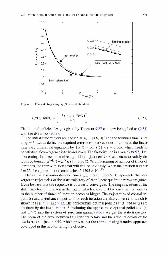
9.3 Finite Horizon Zero-Sum Games for a Class of Nonlinear Systems 371
Fig. 9.10 The state trajectory x1(t) of each iteration
k(x(t),w(t))=[−3x1(t)+ 5w(t)
w(t)
]. (9.57)
The optimal policies designs given by Theorem 9.27 can now be applied to (9.31)with the dynamics (9.57).
The initial state vectors are chosen as x0 = [0.6,0]T and the terminal time is setto tf = 5. Let us define the required error norm between the solutions of the lineartime-vary differential equations by ‖xi(t)− xi−1(t)‖ < ε = 0.005, which needs tobe satisfied if convergence is to be achieved. The factorization is given by (9.57). Im-plementing the present iterative algorithm, it just needs six sequences to satisfy therequired bound, ‖x[6](t)−x[5](t)‖ = 0.0032. With increasing of number of times ofiterations, the approximation error will reduce obviously. When the iteration numberi = 25, the approximation error is just 5.1205 × 10⁻¹⁰.
Define the maximum iteration times imax = 25. Figure 9.10 represents the con-vergence trajectories of the state trajectory of each linear quadratic zero-sum game.It can be seen that the sequence is obviously convergent. The magnifications of thestate trajectories are given in the figure, which shows that the error will be smalleras the number of times of iteration becomes bigger. The trajectories of control in-put u(t) and disturbance input w(t) of each iteration are also convergent, which isshown in Figs. 9.11 and 9.12. The approximate optimal policies u∗(t) and w∗(t) areobtained by the last iteration. Substituting the approximate optimal policies u∗(t)and w∗(t) into the system of zero-sum games (9.56), we get the state trajectory.The norm of the error between this state trajectory and the state trajectory of thelast iteration is just 0.0019, which proves that the approximating iterative approachdeveloped in this section is highly effective.
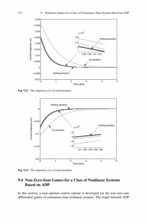
372 9 Nonlinear Games for a Class of Continuous-Time Systems Based on ADP
Fig. 9.11 The trajectory u(t) of each iteration
Fig. 9.12 The trajectory w(t) of each iteration
9.4 Non-Zero-Sum Games for a Class of Nonlinear SystemsBased on ADP
In this section, a near-optimal control scheme is developed for the non-zero-sumdifferential games of continuous-time nonlinear systems. The single network ADP
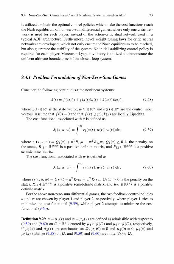
9.4 Non-Zero-Sum Games for a Class of Nonlinear Systems Based on ADP 373
is utilized to obtain the optimal control policies which make the cost functions reachthe Nash equilibrium of non-zero-sum differential games, where only one critic net-work is used for each player, instead of the action-critic dual network used in atypical ADP architecture. Furthermore, novel weight tuning laws for critic neuralnetworks are developed, which not only ensure the Nash equilibrium to be reached,but also guarantee the stability of the system. No initial stabilizing control policy isrequired for each player. Moreover, Lyapunov theory is utilized to demonstrate theuniform ultimate boundedness of the closed-loop system.
9.4.1 Problem Formulation of Non-Zero-Sum Games
Consider the following continuous-time nonlinear systems:
x(t)= f (x(t))+ g(x(t))u(t)+ k(x(t))w(t), (9.58)
where x(t) ∈ Rn is the state vector, u(t) ∈ R
m and d(t) ∈ Rq are the control input
vectors. Assume that f (0)= 0 and that f (x), g(x), k(x) are locally Lipschitz.The cost functional associated with u is defined as
J1(x,u,w)=∫ ∞
t
r1(x(τ ), u(τ ),w(τ))dτ, (9.59)
where r1(x,u,w) = Q1(x) + uTR11u + wTR12w, Q1(x) ≥ 0 is the penalty onthe states, R11 ∈ R
m×m is a positive definite matrix, and R12 ∈ Rq×q is a positive
semidefinite matrix.The cost functional associated with w is defined as
J2(x,u,w)=∫ ∞
t
r2(x(τ ), u(τ ),w(τ))dτ, (9.60)
where r2(x,u,w) = Q2(x)+ uTR21u+wTR22w, Q2(x) ≥ 0 is the penalty on thestates, R21 ∈ R
m×m is a positive semidefinite matrix, and R22 ∈ Rq×q is a positive
definite matrix.For the above non-zero-sum differential games, the two feedback control policies
u and w are chosen by player 1 and player 2, respectively, where player 1 tries tominimize the cost functional (9.59), while player 2 attempts to minimize the costfunctional (9.60).
Definition 9.29 u= μ1(x) and w = μ2(x) are defined as admissible with respect to(9.59) and (9.60) on Ω ∈ R
n, denoted by μ1 ∈ψ(Ω) and μ2 ∈ψ(Ω), respectively,if μ1(x) and μ2(x) are continuous on Ω , μ1(0) = 0 and μ2(0) = 0, μ1(x) andμ2(x) stabilize (9.58) on Ω , and (9.59) and (9.60) are finite, ∀x0 ∈Ω .
374 9 Nonlinear Games for a Class of Continuous-Time Systems Based on ADP
Definition 9.30 The policy set (u∗,w∗) is a Nash equilibrium policy set if the in-equalities
J1(u∗,w∗)≤ J1(u,w
∗),J2(u
∗,w∗)≤ J2(u∗,w) (9.61)
hold for any admissible control policies u and w.
Next, define the Hamilton functions for the cost functionals (9.59) and (9.60)with associated admissible control input u and w, respectively, as follows:
H1(x,u,w)=Q1(x)+ uTR11u+wTR12w
+�J T1 (f (x)+ g(x)u+ k(x)w), (9.62)
H2(x,u,w)=Q2(x)+ uTR21u+wTR22w
+�J T2 (f (x)+ g(x)u+ k(x)w), (9.63)
where �Ji is the partial derivative of the cost function Ji(x,u,w) with respect to x,i = 1,2.
According to the stationarity conditions of optimization, we have
∂H1(x,u,w)/∂u= 0,
∂H2(x,u,w)/∂w = 0.
Therefore, the associated optimal feedback control policies u∗ and w∗ are foundand revealed to be
u∗ = −1
2R−1
11 gT(x)�J1, (9.64)
w∗ = −1
2R−1
22 kT(x)�J2. (9.65)
The optimal feedback control policies u∗ and w∗ provide a Nash equilibrium for thenon-zero-sum differential games among all the feedback control policies.
Considering H1(x,u∗,w∗) = 0 and H2(x,u
∗,w∗) = 0, and substituting the op-timal feedback control policy (9.64) and (9.65) into the Hamilton functions (9.62)and (9.63), we have
Q1(x)−1
4�J T
1 g(x)R−111 g
T(x)�J1 +�J T1 f (x)
+ 1
4�J T
2 k(x)R−122 R12R
−122 k
T(x)�J2
− 1
2�J T
1 k(x)R−122 k
T(x)�J2 = 0, (9.66)
9.4 Non-Zero-Sum Games for a Class of Nonlinear Systems Based on ADP 375
Q2(x)−1
4�J T
2 k(x)R−122 k
T(x)�J2 +�J T2 f (x)
+ 1
4�J T
1 g(x)R−111 R21R
−111 g
T(x)�J1
− 1
2�J T
2 g(x)R−111 g
T(x)�J1 = 0. (9.67)
If the coupled HJ equations (9.66) and (9.67) can be solved for the optimal valuefunctions J1(x,u
∗,w∗) and J2(x,u∗,w∗), the optimal control can then be imple-
mented by using (9.64) and (9.65). However, these equations are generally difficultor impossible to solve due to their inherently nonlinear nature. To overcome thisdifficulty, a near-optimal control scheme is developed to learn the solution of cou-pled HJ equations online using a single network ADP in order to obtain the optimalcontrol policies.
Before presenting the near-optimal control scheme, the following lemma is re-quired.
Lemma 9.31 Given the system (9.58) with associated cost functionals (9.59) and(9.60) and the optimal feedback control policies (9.64) and (9.65). For player i,i = 1,2, let Li(x) be a continuously differentiable, radially unbounded Lyapunovcandidate such that Li = �LT
i x = �LTi (f (x)+ g(x)u∗ + k(x)w∗) < 0, with �Li
being the partial derivative of Li(x) with respect to x. Moreover, let Qi(x) ∈ Rn×n
be a positive definite matrix satisfying ‖Qi(x)‖ = 0 if and only if ‖x‖ = 0 andQimin ≤ ‖Qi(x)‖ ≤ Qimax for ‖χmin‖ ≤ ‖x‖ ≤ χmax with positive constants Qimin,Qimax, χmin, χmax. In addition, let Qi(x) satisfy limx→∞ Qi(x)= ∞ as well as
�J ∗Ti Qi(x)�Li = ri(x,u
∗,w∗). (9.68)
Then the following relation holds:
�LTi (f (x)+ g(x)u∗ + k(x)w∗)= −�LT
i Qi(x)�Li. (9.69)
Proof When the optimal control u∗ and w∗ in (9.64) and (9.65) are applied to thenonlinear system (9.58), the value function Ji(x,u∗,w∗) becomes a Lyapunov func-tion, i = 1,2. Then, for i = 1,2, differentiating the value function Ji(x,u∗,w∗) withrespect to t , we have
J ∗i = �J ∗T
i (f (x)+ g(x)u∗ + k(x)w∗)= −ri(x,u
∗,w∗). (9.70)
Using (9.68), (9.70) can be rewritten as
(f (x)+ g(x)u∗ + k(x)w∗)= − (�J ∗i �J ∗T
i )−1�J ∗i ri(x, u
∗,w∗)
= − (�J ∗i �J ∗T
i )−1�J ∗i �J ∗T
i Qi(x)�Li
= − Qi(x)�Li. (9.71)
376 9 Nonlinear Games for a Class of Continuous-Time Systems Based on ADP
Next, multiplying both sides of (9.71) by �LTi , (9.69) can be obtained.
This completes the proof. �
9.4.2 Optimal Control of Nonlinear Non-Zero-Sum Games Basedon ADP
To begin the development, we rewrite the cost functions (9.59) and (9.60) by NNsas
J1(x)=WTc1φ1(x)+ ε1, (9.72)
J2(x)=WTc2φ2(x)+ ε2, (9.73)
where Wi , φi(x), and εi are the critic NN ideal constant weights, the critic NNactivation function vector and the NN approximation error for player i, i = 1,2,respectively.
The derivative of the cost functions with respect to x can be derived as
�J1 = �φT1Wc1 +�ε1, (9.74)
�J2 = �φT2Wc2 +�ε2, (9.75)
where �φi � ∂φi(x)/∂x, �εi � ∂εi/∂x, i = 1,2.Using (9.74) and (9.75), the optimal feedback control policies (9.64) and (9.65)
can be rewritten as
u∗ = −1
2R−1
11 gT(x)�φT
1Wc1 − 1
2R−1
11 gT(x)�ε1, (9.76)
w∗ = −1
2R−1
22 kT(x)�φT
2Wc2 − 1
2R−1
22 kT(x)�ε2, (9.77)
and the coupled HJ equations (9.66) and (9.67) can be rewritten as
Q1(x)−1
4WT
c1�φ1D1�φT1Wc1 +WT
c1�φ1f (x)
+ 1
4WT
c2�φ2S2�φ2TWc2 − 1
2WT
c1�φ1D2�φT2Wc2 − εHJ1 = 0, (9.78)
Q2(x)−1
4WT
c2�φ2D2�φT2Wc2 +WT
c2�φ2f (x)
+ 1
4WT
c1�φ1S1�φ1TWc1 − 1
2WT
c2�φ2D1�φT1Wc1 − εHJ2 = 0, (9.79)
9.4 Non-Zero-Sum Games for a Class of Nonlinear Systems Based on ADP 377
where
D1 =g(x)R−111 g
T(x),
D2 = k(x)R−122 k
T(x),
S1 =g(x)R−111 R21R
−111 g
T(x),
S2 = k(x)R−122 R12R
−122 k
T(x). (9.80)
The residual error due to the NN approximation for player 1 is
εHJ1 = −�εT1
(f (x)− 1
2D1(�φT
1Wc1 +�ε1)
− 1
2D2(�φT
2Wc2 +�ε2)
)− 1
4�εT
1D1�ε1 + 1
2WT
c1�φ1D2�ε2
− 1
2�εT
2 S2�φT2Wc2 − 1
4�εT
2 S2�ε2. (9.81)
The residual error due to the NN approximation for player 2 is
εHJ2 = −�εT2
(f (x)− 1
2D1(�φT
1Wc1 +�ε1)
− 1
2D2(�φT
2Wc2 +�ε2)
)− 1
4�εT
2D2�ε2 + 1
2WT
c2�φ2D1�ε1
− 1
2�εT
2 S1�φT1Wc2 − 1
4�εT
1 S1�ε1. (9.82)
Let Wc1 and Wc2 be the estimates of Wc1 and Wc2, respectively. Then we havethe estimates of V1(x) and V2(x) as follows:
J1(x)= WTc1φ1(x), (9.83)
J2(x)= WTc2φ2(x). (9.84)
Substituting (9.83) and (9.84) into (9.64) and (9.65), respectively, the estimates ofoptimal control policies can be written as
u= −1
2R−1
11 gT(x)�φT
1 Wc1, (9.85)
w = −1
2R−1
22 kT(x)�φT
2 Wc2. (9.86)
Applying (9.85) and (9.86) to the system (9.58), we have the closed-loop systemdynamics as follows:
x = f (x)− D1�φT1 Wc1
2− D2�φT
2 Wc2
2. (9.87)
378 9 Nonlinear Games for a Class of Continuous-Time Systems Based on ADP
Substituting (9.83) and (9.84) into (9.62) and (9.63), respectively, the approxi-mate Hamilton functions can be derived as follows:
H1(x, Wc1, Wc2)=Q1(x)− 1
4WT
c1�φ1D1�φT1 Wc1 + WT
c1�φ1f (x)
+ 1
4WT
c2�φ2S2�φT2 Wc2 − 1
2WT
c1�φ1D2�φT2 Wc2
= e1, (9.88)
H2(x, Wc1, Wc2)=Q2(x)− 1
4WT
c2�φ2D2�φT2 Wc2 + WT
c2�φ2f (x)
+ 1
4WT
c1�φ1S1�φT1 Wc1 − 1
2WT
c2�φ2D1�φT1 Wc1
= e2. (9.89)
It is desired to select Wc1 and Wc2 to minimize the squared residual error E =eT
1 e1/2 + eT2 e2/2. Then we have Wc1 → Wc1, Wc2 → Wc2, and e1 → εHJ1, e2 →
εHJ2. In other words, the Nash equilibrium of the non-zero-sum differential gamesof continuous-time nonlinear system (9.58) can be obtained. However, tuning thecritic NN weights to minimize the squared residual error E alone does not ensurethe stability of the nonlinear system (9.58) during the learning process of critic NNs.Therefore, we propose the novel weight tuning laws of critic NNs for two players,which cannot only minimize the squared residual error E but also guarantee thestability of the system as follows:
˙W1 = − α1
σ1
ms1
(Q1(x)− 1
4WT
c1�φ1D1�φT1 Wc1
+ WTc1�φ1f (x)+ 1
4WT
c2�φ2S2�φT2 Wc2 − 1
2WT
c1�φ1D2�φT2 Wc2
)
+ α1
4�φ1D1�φT
1 Wc1σT
1
ms1
Wc1 + α2
4�φ1S1�φT
1 Wc1σT
2
ms2
Wc2
+Σ(x, u, w)
(α1�φ1D1�L1
2+ α1�φ1D1�L2
2
)
− α1(F1Wc1 − F2σT1 Wc1), (9.90)
˙W2 = − α2
σ2
ms2
(Q2(x)− 1
4WT
c2�φ2D2�φT2 Wc2
+ WTc2�φ2f (x)+ 1
4WT
c1�φ1S1�φT1 Wc1 − 1
2WT
c2�φ2D1�φT1 Wc1
)
9.4 Non-Zero-Sum Games for a Class of Nonlinear Systems Based on ADP 379
+ α2
4�φ2D2�φT
2 Wc2σT
2
ms2
Wc2 + α2
4�φ2S2�φT
2 Wc2σT
1
ms1
Wc1
+Σ(x, u, w)
(α2�φ2D2�L2
2+ α2�φ2D2�L1
2
)
− α2(F3Wc2 − F4σT2 Wc2), (9.91)
where σi = σi/(σTi σi + 1), σi = �φi(f (x) − D1�φT
1 Wc1/2 − D2�φT2 Wc2/2),
msi = σTi σi + 1, αi > 0 is the adaptive gain, �Li is described in Lemma 9.31,
i = 1,2. F1, F2, F3, and F4 are design parameters. The operator Σ(x, u, w) is givenby
Σ(x, u, w)={
0 if �L1x ≤ 0 and �L2x ≤ 0,1 else,
(9.92)
where x is given as (9.87).
Remark 9.32 The first terms in (9.90) and (9.91) are utilized to minimize thesquared residual error E and derived by using a normalized gradient descent al-gorithm. The other terms are utilized to guarantee the stability of the closed-loopsystem while the critic NNs learn the optimal cost functions and are derived byfollowing Lyapunov stability analysis. The operator Σ(x, u, w) is selected basedon the Lyapunov’s sufficient condition for stability, which means that the state x isstable if Li(x) > 0 and �Lix < 0 for player i, i = 1,2. When the system (9.58)is stable, the operator Σ(x, u, w) = 0 and it will not take effect. When the system(9.58) is unstable, the operator Σ(x, u, w)= 1 and it will be activated. Therefore, noinitial stabilizing control policies are needed due to the introduction of the operatorΣ(x, u, w).
Remark 9.33 From (9.88) and (9.89), it can be seen that the approximate Hamiltonfunctions H1(x, Wc1, Wc2) = e1 = 0 and H2(x, Wc1, Wc2) = e2 = 0 when x = 0.For this case, the tuning laws of critic NN weights for two players (9.90) and (9.91)cannot achieve the purpose of optimization anymore. This can be considered as apersistency of the requirement of excitation for the system states. Therefore, the sys-tem states must be persistently excited enough for minimizing the squared residualerrors E to drive the critic NN weights toward their ideal values. In order to satisfythe persistent excitation condition, probing noise is added to the control input.
Define the weight estimation errors of critic NNs for two players to be Wc1 =Wc1 − Wc1 and Wc2 =Wc2 − Wc2, respectively. From (9.78) and (9.79), we observethat
Q1(x)= 1
4WT
c1�φ1D1�φT1Wc1 −WT
c1�φ1f (x)− 1
4WT
c2�φ2S2�φ2TWc2
+ 1
2WT
c1�φ1D2�φT2Wc2 + εHJ1, (9.93)
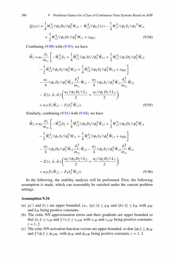
380 9 Nonlinear Games for a Class of Continuous-Time Systems Based on ADP
Q2(x)= 1
4WT
c2�φ2D2�φT2Wc2 −WT
c2�φ2f (x)− 1
4WT
c1�φ1S1�φ1TWc1
+ 1
2WT
c2�φ2D1�φT1Wc1 + εHJ2. (9.94)
Combining (9.90) with (9.93), we have
˙W1 =α1
σ1
ms1
[−WT
c1σ1 + 1
4WT
c1�φ1D1�φT1 Wc1 + 1
2WT
c1�φ1D2�φT2 Wc2
− 1
2WT
c2�φ2S2�φT2Wc2 + 1
4WT
c2�φ2S2�φT2 Wc2 + εHJ1
]
− α1
4�φ1D1�φT
1 Wc1σT
1
ms1
Wc1 − α2
4�φ1S1�φT
1 Wc1σT
2
ms2
Wc2
−Σ(x, u, w)
(α1�φ1D1�L1
2+ α1�φ1D1�L2
2
)
+ α1(F1Wc1 − F2σT1 Wc1). (9.95)
Similarly, combining (9.91) with (9.94), we have
˙W2 =α2
σ2
ms2
[−WT
c2σ2 + 1
4WT
c2�φ2D2�φT2 Wc2 + 1
2WT
c2�φ2D1�φT1 Wc1
− 1
2WT
c1�φ1S1�φT1Wc1 + 1
4WT
c1�φ1S1�φT1 Wc1 + εHJ2
]
− α2
4�φ2D2�φT
2 Wc2σT
2
ms2
Wc2 − α2
4�φ2S2�φT
2 Wc2σT
1
ms1
Wc1
−Σ(x, u, w)
(α2�φ2D2�L2
2+ α2�φ2D2�L1
2
)
+ α2(F3Wc2 − F4σT2 Wc2). (9.96)
In the following, the stability analysis will be performed. First, the followingassumption is made, which can reasonably be satisfied under the current problemsettings.
Assumption 9.34
(a) g(·) and k(·) are upper bounded, i.e., ‖g(·)‖ ≤ gM and ‖k(·)‖ ≤ kM with gMand kM being positive constants.
(b) The critic NN approximation errors and their gradients are upper bounded sothat ‖εi‖ ≤ εiM and ‖�εi‖ ≤ εidM with εiM and εidM being positive constants,i = 1,2.
(c) The critic NN activation function vectors are upper bounded, so that ‖φi‖ ≤ φiMand ‖�φi‖ ≤ φidM , with φiM and φidM being positive constants, i = 1,2.
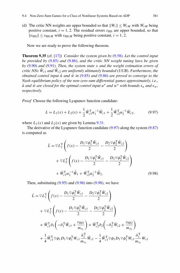
9.4 Non-Zero-Sum Games for a Class of Nonlinear Systems Based on ADP 381
(d) The critic NN weights are upper bounded so that ‖Wi‖ ≤WiM with WiM beingpositive constant, i = 1,2. The residual errors εHJi are upper bounded, so that‖εHJi‖ ≤ εHJiM with εHJiM being positive constant, i = 1,2.
Now we are ready to prove the following theorem.
Theorem 9.35 (cf. [17]) Consider the system given by (9.58). Let the control inputbe provided by (9.85) and (9.86), and the critic NN weight tuning laws be givenby (9.90) and (9.91). Then, the system state x and the weight estimation errors ofcritic NNs Wc1 and Wc2 are uniformly ultimately bounded (UUB). Furthermore, theobtained control input u and w in (9.85) and (9.86) are proved to converge to theNash equilibrium policy of the non-zero-sum differential games approximately, i.e.,u and w are closed for the optimal control input u∗ and w∗ with bounds εu and εw ,respectively.
Proof Choose the following Lyapunov function candidate:
L= L1(x)+L2(x)+ 1
2WT
c1α−11 Wc1 + 1
2WT
c2α−12 Wc2, (9.97)
where L1(x) and L2(x) are given by Lemma 9.31.The derivative of the Lyapunov function candidate (9.97) along the system (9.87)
is computed as
L=�LT1
(f (x)− D1�φT
1 Wc1
2− D2�φT
2 Wc2
2
)
+�LT2
(f (x)− D1�φT
1 Wc1
2− D2�φT
2 Wc2
2
)
+ WTc1α
−11
˙W1 + WT
c2α−12
˙W2. (9.98)
Then, substituting (9.95) and (9.96) into (9.98), we have
L=�LT1
(f (x)− D1�φT
1 Wc1
2− D2�φT
2 Wc2
2
)
+�LT2
(f (x)− D1�φT
1 Wc1
2− D2�φT
2 Wc2
2
)
+ WTc1σ1
(−σT
1 Wc1 + εHJ1
ms1
)+ WT
c2σ2
(−σT
2 Wc2 + εHJ2
ms2
)
+ 1
4WT
c1�φ1D1�φT1Wc1
σT1
ms1
Wc1 − 1
4WT
c1�φ1D1�φT1Wc1
σT1
ms1
Wc1
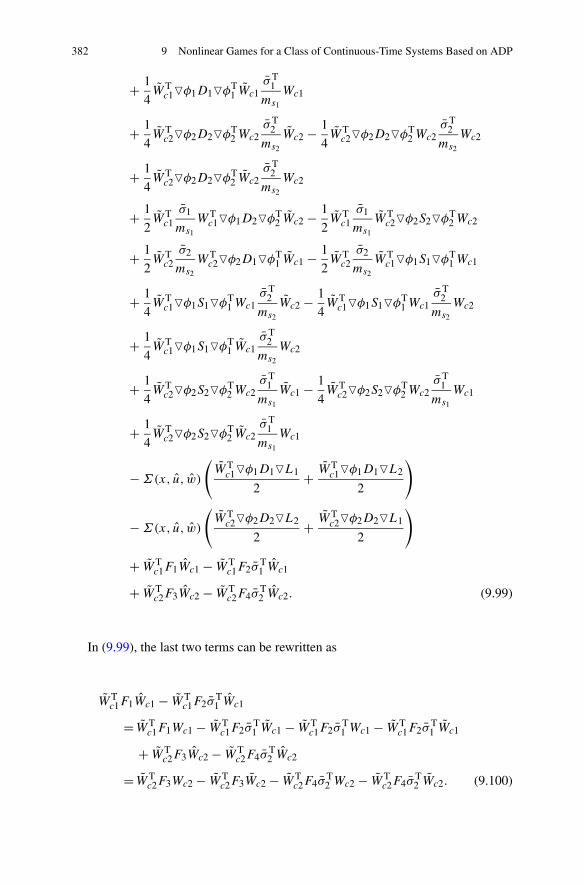
382 9 Nonlinear Games for a Class of Continuous-Time Systems Based on ADP
+ 1
4WT
c1�φ1D1�φT1 Wc1
σT1
ms1
Wc1
+ 1
4WT
c2�φ2D2�φT2Wc2
σT2
ms2
Wc2 − 1
4WT
c2�φ2D2�φT2Wc2
σT2
ms2
Wc2
+ 1
4WT
c2�φ2D2�φT2 Wc2
σT2
ms2
Wc2
+ 1
2WT
c1σ1
ms1
WTc1�φ1D2�φT
2 Wc2 − 1
2WT
c1σ1
ms1
WTc2�φ2S2�φT
2Wc2
+ 1
2WT
c2σ2
ms2
WTc2�φ2D1�φT
1 Wc1 − 1
2WT
c2σ2
ms2
WTc1�φ1S1�φT
1Wc1
+ 1
4WT
c1�φ1S1�φT1Wc1
σT2
ms2
Wc2 − 1
4WT
c1�φ1S1�φT1Wc1
σT2
ms2
Wc2
+ 1
4WT
c1�φ1S1�φT1 Wc1
σT2
ms2
Wc2
+ 1
4WT
c2�φ2S2�φT2Wc2
σT1
ms1
Wc1 − 1
4WT
c2�φ2S2�φT2Wc2
σT1
ms1
Wc1
+ 1
4WT
c2�φ2S2�φT2 Wc2
σT1
ms1
Wc1
−Σ(x, u, w)
(WT
c1�φ1D1�L1
2+ WT
c1�φ1D1�L2
2
)
−Σ(x, u, w)
(WT
c2�φ2D2�L2
2+ WT
c2�φ2D2�L1
2
)
+ WTc1F1Wc1 − WT
c1F2σT1 Wc1
+ WTc2F3Wc2 − WT
c2F4σT2 Wc2. (9.99)
In (9.99), the last two terms can be rewritten as
WTc1F1Wc1 − WT
c1F2σT1 Wc1
= WTc1F1Wc1 − WT
c1F2σT1 Wc1 − WT
c1F2σT1 Wc1 − WT
c1F2σT1 Wc1
+ WTc2F3Wc2 − WT
c2F4σT2 Wc2
= WTc2F3Wc2 − WT
c2F3Wc2 − WTc2F4σ
T2 Wc2 − WT
c2F4σT2 Wc2. (9.100)
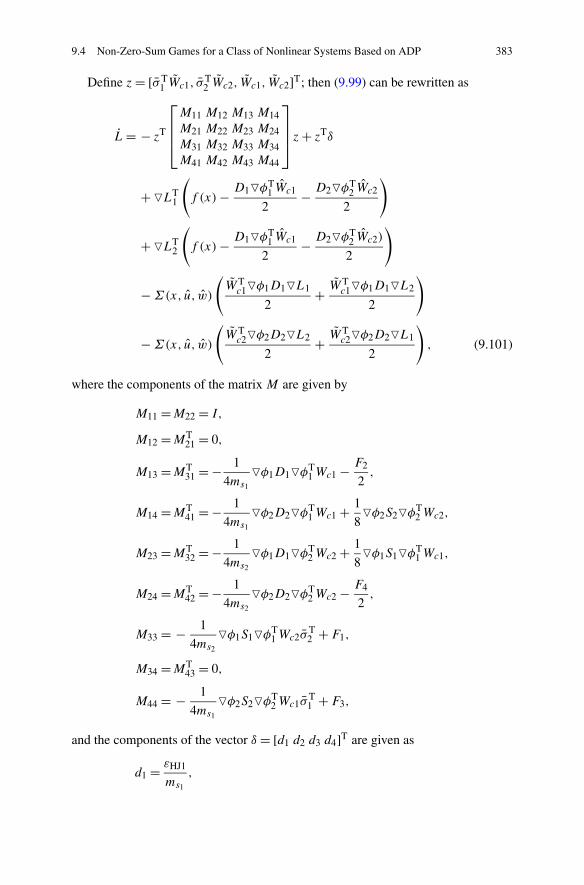
9.4 Non-Zero-Sum Games for a Class of Nonlinear Systems Based on ADP 383
Define z= [σT1 Wc1, σ
T2 Wc2, Wc1, Wc2]T; then (9.99) can be rewritten as
L= − zT
⎡
⎢⎢⎣
M11 M12 M13 M14M21 M22 M23 M24M31 M32 M33 M34M41 M42 M43 M44
⎤
⎥⎥⎦ z+ zTδ
+�LT1
(f (x)− D1�φT
1 Wc1
2− D2�φT
2 Wc2
2
)
+�LT2
(f (x)− D1�φT
1 Wc1
2− D2�φT
2 Wc2)
2
)
−Σ(x, u, w)
(WT
c1�φ1D1�L1
2+ WT
c1�φ1D1�L2
2
)
−Σ(x, u, w)
(WT
c2�φ2D2�L2
2+ WT
c2�φ2D2�L1
2
), (9.101)
where the components of the matrix M are given by
M11 =M22 = I,
M12 =MT21 = 0,
M13 =MT31 = − 1
4ms1
�φ1D1�φT1Wc1 − F2
2,
M14 =MT41 = − 1
4ms1
�φ2D2�φT1Wc1 + 1
8�φ2S2�φT
2Wc2,
M23 =MT32 = − 1
4ms2
�φ1D1�φT2Wc2 + 1
8�φ1S1�φT
1Wc1,
M24 =MT42 = − 1
4ms2
�φ2D2�φT2Wc2 − F4
2,
M33 = − 1
4ms2
�φ1S1�φT1Wc2σ
T2 + F1,
M34 =MT43 = 0,
M44 = − 1
4ms1
�φ2S2�φT2Wc1σ
T1 + F3,
and the components of the vector δ = [d1 d2 d3 d4]T are given as
d1 = εHJ1
ms1
,
384 9 Nonlinear Games for a Class of Continuous-Time Systems Based on ADP
d2 = εHJ2
ms2
,
d3 = − 1
4ms1
�φ1D1�φT1Wc1σ
T1 Wc1
− 1
4ms2
�φ1S1�φT1Wc1σ
T2 Wc2 + F1Wc1 − F2σ
T1 Wc1,
d4 = − 1
4ms2
�φ2D2�φT2Wc2σ
T2 Wc2
− 1
4ms1
�φ2S2�φT2Wc2σ
T1 Wc1 + F3Wc2 − F4σ
T2 Wc2.
According to Assumption 9.34 and observing the facts that σ1 < 1 and σ2 < 1, itcan be concluded that δ is bounded by δM . Let the parameters F1, F2, F3, and F4
be chosen such that M > 0. Then, taking the upper bounds of (9.101) reveals
L≤�L1
(f (x)− D1�φT
1 Wc1
2− D2�φT
2 Wc2
2
)
+�L2
(f (x)− D1�φT
1 Wc1
2− D2�φT
2 Wc2
2
)
− ‖z‖2σmin(M)+ ‖z‖δM
−Σ(x, u, w)
(WT
c1�φ1D1�L1
2+ WT
c1�φ1D1�L2
2
)
−Σ(x, u, w)
(WT
c2�φ2D2�L2
2+ WT
c2�φ2D2�L1
2
). (9.102)
Now, the cases of Σ(x, u, w)= 0 and Σ(x, u, w)= 1 will be considered.(1) When Σ(x, u, w) = 0, the first two terms are less than zero. Noting that
‖x‖> 0 as guaranteed by the persistent excitation condition and using the operatordefined in (9.92), it can be ensured that there exists a constant xmin satisfying 0 <xmin < ‖x‖. Then (9.102) becomes
L≤ − xmin(‖�L1‖ + ‖�L2‖)− ‖z‖2σmin(M)+ ‖z‖δM
= − xmin(‖�L1‖+‖�L2‖)−σmin(M)
(‖z‖− δM
2σmin(M)
)2
+ δ2M
4σmin(M). (9.103)
9.4 Non-Zero-Sum Games for a Class of Nonlinear Systems Based on ADP 385
Given that the following inequalities:
‖�L1‖ ≥ δ2M
4σmin(M)xmin� B�L1, (9.104)
or
‖�L2‖ ≥ δ2M
4σmin(M)xmin� B�L2, (9.105)
or
‖z‖ ≥ δM
σmin(M)� Bz (9.106)
hold, then L < 0. Therefore, using Lyapunov theory, it can be concluded that‖�L1‖, ‖�L2‖ and ‖z‖ are UUB.
(2) When Σ(x, u, w) = 1, it implies that the feedback control input (9.85) and(9.86) may not stabilize the system (9.58). Adding and subtracting �LT
1D1ε1/2 +�LT
2D2ε2/2 to the right hand side of (9.102), and using (9.64), (9.65), and (9.80),we have
L≤�LT1 (f (x)+ g(x)u∗ + k(x)w∗)+�LT
2 (f (x)+ g(x)u∗ + k(x)w∗)
+ 1
2�L1D1�ε1 + 1
2�L2D2�ε2 + 1
2�L1D2�ε2 + 1
2�L2D1�ε1
− σmin(M)
(‖z‖ − δM
2σmin(M)
)2
+ δ2M
4σmin(M). (9.107)
According to Assumption 9.34, Di is bounded by DiM , where DiM is a knownconstant, i = 1,2. Using Lemma 9.31 and recalling the boundedness of �ε1, �ε2,and δ, (9.107) can be rewritten as
L≤ − Q1 min‖�L1‖2 − Q2 min‖�L2‖2 + 1
2‖�L1‖D1Mε1dM
+ 1
2‖�L2‖D2Mε2dM + 1
2‖�L1‖D2Mε2dM
+ 1
2‖�L2‖D1Mε1dM − σmin(M)
(‖z‖ − δM
2σmin(M)
)2
+ δ2M
4σmin(M)
≤ − 1
2Q1 min‖�L1‖2− 1
2Q2 min‖�L2‖2−σmin(M)
(‖z‖− δM
2σmin(M)
)2
+η,
(9.108)
where
η = D21Mε2
1dM
4Q1 min+ D2
2Mε22dM
4Q2 min+ D2
2Mε22dM
4Q1 min+ D2
1Mε21dM
4Q2 min+ δ2
M
4σmin(M).
386 9 Nonlinear Games for a Class of Continuous-Time Systems Based on ADP
Given that the following inequalities:
‖�L1‖>√
2η
Q1 min� B ′
�L1, (9.109)
or
‖�L2‖>√
2η
Q2 min� B ′
�L2, (9.110)
or
‖z‖>√
η
σmin(M)+ δM
2σmin(M)� B ′
z (9.111)
hold, then L < 0. Therefore, using Lyapunov theory, it can be concluded that‖�L1‖, ‖�L2‖, and ‖z‖ are UUB.
In summary, for the cases Σ(x, u, w) = 0 and Σ(x, u, w) = 1, if inequalities‖�L1‖ > max(B�L1 ,B
′�L1
) � B�L1 , or ‖�L2‖ > max(B�L2 ,B′�L2
) � B�L2 or
‖z‖> max(Bz,B′z)� Bz hold, then L < 0. Therefore, we can conclude that ‖�L1‖,
‖�L2‖ and ‖z‖ are bounded by B�L1 , B�L2 , and Bz, respectively. According toLemma 9.31, the Lyapunov candidates �L1 and �L2 are radially unbounded andcontinuously differentiable. Therefore, the boundedness of ‖�L1‖ and ‖�L2‖ im-plies the boundedness of ‖x‖. Specifically, ‖x‖ is bounded by Bx = max(B1x,B2x),where B1x and B2x are determined by B�L1 and B�L2 , respectively. Besides, notethat if any component of z exceeds the bound, i.e., ‖Wc1‖ > Bz or ‖Wc2‖ > Bz or‖σT
1 Wc1‖ > Bz or ‖σT2 Wc2‖ > Bz, the ‖z‖ are bounded by Bz, which implies that
the critic NN weight estimation errors ‖Wc1‖ and ‖Wc2‖ are also bounded by Bz.Next, we will prove ‖u− u∗‖ ≤ εu and ‖w −w∗‖ ≤ εw . From (9.64) and (9.85)
and recalling the boundedness of ‖�φ1‖ and ‖Wc1‖, we have
‖u− u∗‖ ≤∥∥∥∥−
1
2R−1
11 gT�φT
1 Wc1
∥∥∥∥
≤ λmax(R−111 )�φ1MBz
� εu. (9.112)
Similarly, from (9.65) and (9.86) and recalling the boundedness of ‖�φ2‖ and‖Wc2‖, we obtain ‖w −w∗‖ ≤ εw .
This completes the proof. �
Remark 9.36 In [10], each player needs two NNs consisting of a critic NN and anaction NN to implement the online learning algorithm. By contrast with [10], onlyone critic NN is required for each player, the action NN is eliminated, resulting in asimpler architecture, and less computational burden.
9.4 Non-Zero-Sum Games for a Class of Nonlinear Systems Based on ADP 387
Remark 9.37 In Remark 3 of [10] one pointed out that the NN weights can be initial-ized randomly but non-zero. That is because the method proposed in [10] requiresinitial stabilizing control policies for guaranteeing the stability of the system. Bycontrast, no initial stabilizing control policies are needed by adding an operator,which is selected by the Lyapunov’s sufficiency condition for stability, on the criticNN weight tuning law for each player in this subsection.
9.4.3 Simulations
Example 9.38 An example is provided to demonstrate the effectiveness of thepresent control scheme.
Consider the affine nonlinear system as follows:
x = f (x)+ g(x)u+ k(x)w, (9.113)
where
f (x)=[
x2 − 2x1
−x2 − 0.5x1 + 0.25x2(cos(2x1 + 2))2 + 0.25x2(sin(4x21)+ 2)2
],
(9.114)
g(x)=[
0cos(2x1 + 2)
], k(x)=
[0
sin(4x21)+ 2)
]. (9.115)
The cost functionals for player 1 and player 2 are defined by (9.59) and (9.60),respectively, where Q1(x) = 2xTx, R11 = R12 = 2I , Q2(x) = xTx, R21 = R22 =2I , and I denotes an identity matrix of appropriate dimensions.
For player 1, the optimal cost function is V ∗1 (x)= 0.25x2
1 + x22 . For player 2, the
optimal cost function is V ∗2 (x)= 0.25x2
1 + 0.5x22 . The activation functions of critic
NNs of two players are selected as φ1 = φ2 = [x21 , x1x2, x
22 ]T. Then, the optimal
values of the critic NN weights for player 1 are Wc1 = [0.5,0,1]T. The optimalvalues of the critic NN weights for player 2 are Wc2 = [0.25,0,0.5]T. The estimatesof the critic NN weights for two players are denoted Wc1 = [W11,W12,W13]T andWc2 = [W21,W22,W23]T, respectively. The adaptive gains for the critic NNs areselected as a1 = 1 and a2 = 1, and the design parameters are selected as F1 = F2 =F3 = F4 = 10I . All NN weights are initialized to zero, which means that no initialstabilizing control policies are needed for implementing the present control scheme.The system state is initialized as [0.5,0.2]T. To maintain the excitation condition,probing noise is added to the control input for the first 250 s.
After simulation, the trajectories of the system states are shown in Fig. 9.13.The convergence trajectories of the critic NN weights for player 1 are shown inFig. 9.14, from which we see that the critic NN weights for player 1 finally convergeto [0.4490,0.0280,0.9777]T. The convergence trajectories of the critic NN weightsfor player 2 are shown in Fig. 9.15, from which we see that the critic NN weights for
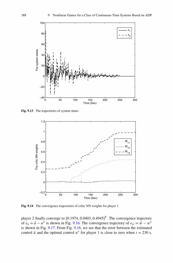
388 9 Nonlinear Games for a Class of Continuous-Time Systems Based on ADP
Fig. 9.13 The trajectories of system states
Fig. 9.14 The convergence trajectories of critic NN weights for player 1
player 2 finally converge to [0.1974,0.0403,0.4945]T. The convergence trajectoryof eu = u− u∗ is shown in Fig. 9.16. The convergence trajectory of ew = w −w∗is shown in Fig. 9.17. From Fig. 9.16, we see that the error between the estimatedcontrol u and the optimal control u∗ for player 1 is close to zero when t = 230 s.
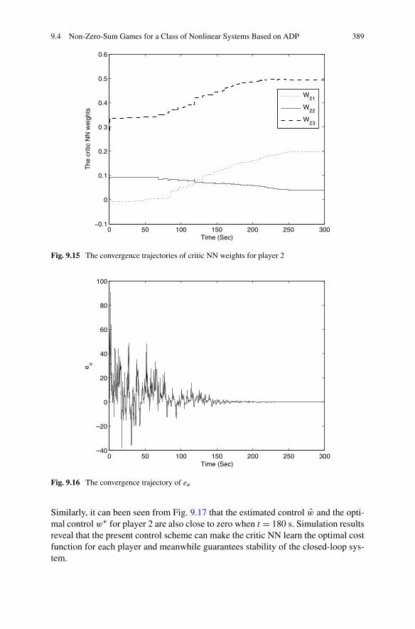
9.4 Non-Zero-Sum Games for a Class of Nonlinear Systems Based on ADP 389
Fig. 9.15 The convergence trajectories of critic NN weights for player 2
Fig. 9.16 The convergence trajectory of eu
Similarly, it can been seen from Fig. 9.17 that the estimated control w and the opti-mal control w∗ for player 2 are also close to zero when t = 180 s. Simulation resultsreveal that the present control scheme can make the critic NN learn the optimal costfunction for each player and meanwhile guarantees stability of the closed-loop sys-tem.
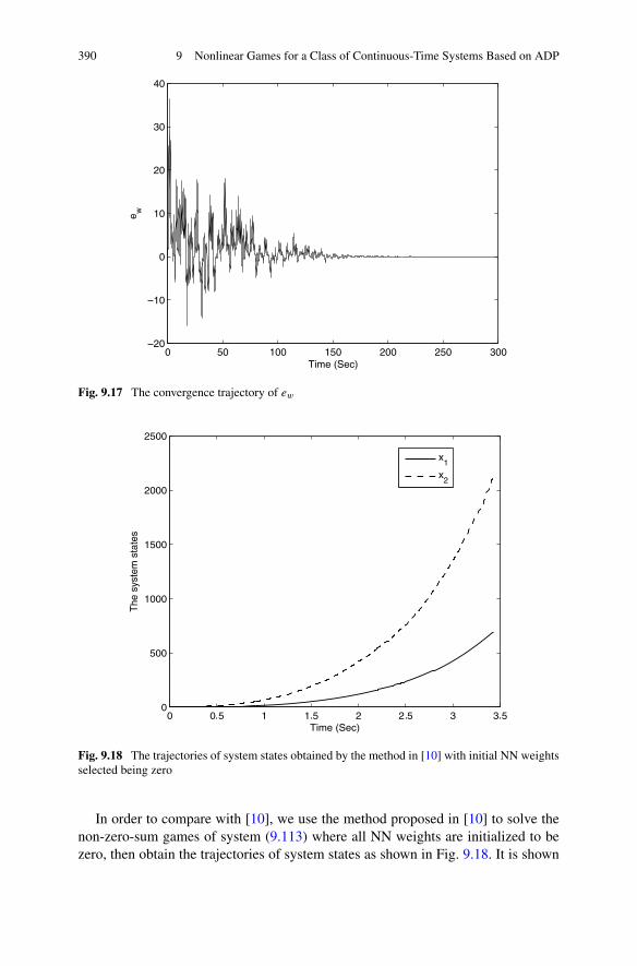
390 9 Nonlinear Games for a Class of Continuous-Time Systems Based on ADP
Fig. 9.17 The convergence trajectory of ew
Fig. 9.18 The trajectories of system states obtained by the method in [10] with initial NN weightsselected being zero
In order to compare with [10], we use the method proposed in [10] to solve thenon-zero-sum games of system (9.113) where all NN weights are initialized to bezero, then obtain the trajectories of system states as shown in Fig. 9.18. It is shown
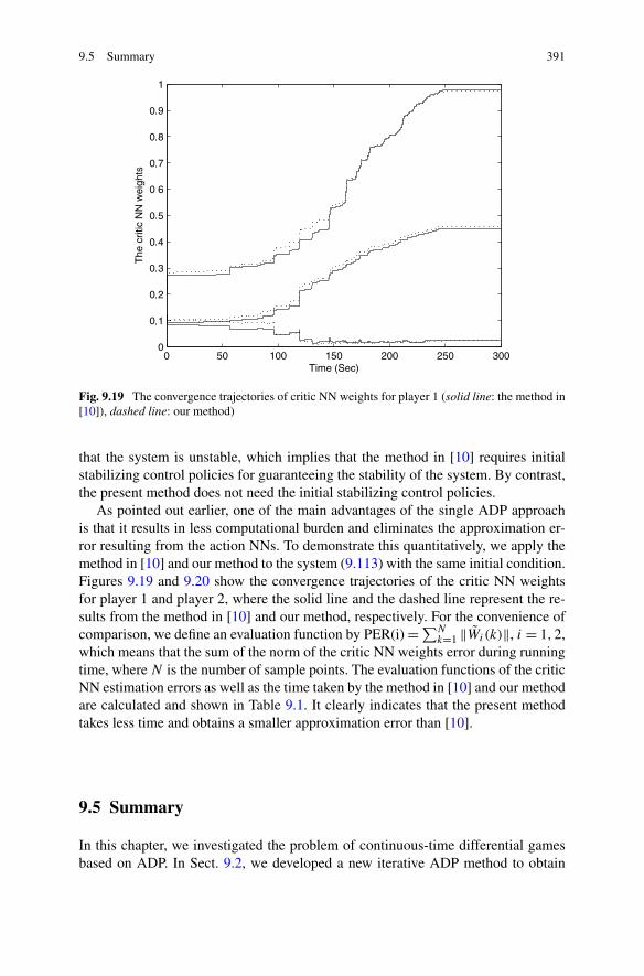
9.5 Summary 391
Fig. 9.19 The convergence trajectories of critic NN weights for player 1 (solid line: the method in[10]), dashed line: our method)
that the system is unstable, which implies that the method in [10] requires initialstabilizing control policies for guaranteeing the stability of the system. By contrast,the present method does not need the initial stabilizing control policies.
As pointed out earlier, one of the main advantages of the single ADP approachis that it results in less computational burden and eliminates the approximation er-ror resulting from the action NNs. To demonstrate this quantitatively, we apply themethod in [10] and our method to the system (9.113) with the same initial condition.Figures 9.19 and 9.20 show the convergence trajectories of the critic NN weightsfor player 1 and player 2, where the solid line and the dashed line represent the re-sults from the method in [10] and our method, respectively. For the convenience ofcomparison, we define an evaluation function by PER(i) =∑N
k=1 ‖Wi(k)‖, i = 1,2,which means that the sum of the norm of the critic NN weights error during runningtime, where N is the number of sample points. The evaluation functions of the criticNN estimation errors as well as the time taken by the method in [10] and our methodare calculated and shown in Table 9.1. It clearly indicates that the present methodtakes less time and obtains a smaller approximation error than [10].
9.5 Summary
In this chapter, we investigated the problem of continuous-time differential gamesbased on ADP. In Sect. 9.2, we developed a new iterative ADP method to obtain
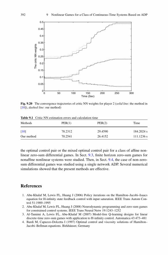
392 9 Nonlinear Games for a Class of Continuous-Time Systems Based on ADP
Fig. 9.20 The convergence trajectories of critic NN weights for player 2 (solid line: the method in[10]), dashed line: our method)
Table 9.1 Critic NN estimation errors and calculation time
Methods PER(1) PER(2) Time
[10] 78.2312 29.4590 184.2024 s
Our method 70.2541 26.4152 111.1236 s
the optimal control pair or the mixed optimal control pair for a class of affine non-linear zero-sum differential games. In Sect. 9.3, finite horizon zero-sum games fornonaffine nonlinear systems were studied. Then, in Sect. 9.4, the case of non-zero-sum differential games was studied using a single network ADP. Several numericalsimulations showed that the present methods are effective.
References
1. Abu-Khalaf M, Lewis FL, Huang J (2006) Policy iterations on the Hamilton–Jacobi–Isaacsequation for H-infinity state feedback control with input saturation. IEEE Trans Autom Con-trol 51:1989–1995
2. Abu-Khalaf M, Lewis FL, Huang J (2008) Neurodynamic programming and zero-sum gamesfor constrained control systems. IEEE Trans Neural Netw 19:1243–1252
3. Al-Tamimi A, Lewis FL, Abu-Khalaf M (2007) Model-free Q-learning designs for lineardiscrete-time zero-sum games with application to H-infinity control. Automatica 43:473–481
4. Bardi M, Capuzzo-Dolcetta I (1997) Optimal control and viscosity solutions of Hamilton–Jacobi–Bellman equations. Birkhäuser, Germany
References 393
5. Birkhäuser (1995) H-infinity optimal control and related minimax design problems: a dynam-ical game approach. Birkhäuser, Berlin
6. Chang HS, Hu J, Fu MC (2010) Adaptive adversial multi-armed bandit approach to two-person zero-sum Markov games. IEEE Trans Autom Control 55:463–468
7. Chen BS, Tseng CS, Uang HJ (2002) Fuzzy differential games for nonlinear stochastic sys-tems: suboptimal approach. IEEE Trans Fuzzy Syst 10:222–233
8. Laraki R, Solan E (2005) The value of zero-sum stopping games in continuous time. SIAM JControl Optim 43:1913–1922
9. Starr AW, Ho YC (1967) Nonzero-sum differential games. J Optim Theory Appl 3:184–20610. Vamvoudakisand KG, Lewis FL (2011) Multi-player non-zero-sum games: online adap-
tive learning solution of coupled Hamilton–Jacobi equations. Automatica. doi:10.1016/j.automatica.2011.03.005
11. Wang X (2008) Numerical solution of optimal control for scaled systems by hybrid functions.Int J Innov Comput Inf Control 4:849–856
12. Wei QL, Zhang HG, Liu DR (2008) A new approach to solve a class of continuous-time non-linear quadratic zero-sum game using ADP. In: Proceedings of IEEE international conferenceon networking, sensing and control, Sanya, China, pp 507–512
13. Wei QL, Zhang HG, Cui LL (2009) Data-based optimal control for discrete-time zero-sumgames of 2-D systems using adaptive critic designs. Acta Autom Sin 35:682–692
14. Wei QL, Zhang HG, Dai J (2009) Model-free multiobjective approximate dynamic program-ming for discrete-time nonlinear systems with general performance index functions. Neuro-computing 7–9:1839–1848
15. Zhang HG, Wei QL, Liu DR (2011) An iterative adaptive dynamic programming method forsolving a class of nonlinear zero-sum differential games. Automatica 47:207–214
16. Zhang X, Zhang HG, Wang XY (2011) A new iteration approach to solve a class of finite-horizon continuous-time nonaffine nonlinear zero-sum game. Int J Innov Comput Inf Control7:597–608
17. Zhang HG, Cui LL, Luo YH (2012) Near-optimal control for non-zero-sum differential gamesof continuous-time nonlinear systems using single network ADP. IEEE Trans Syst Man Cy-bern, Part B, Cybern. doi:10.1109/TSMCB.2012.2203336
Chapter 10Other Applications of ADP
10.1 Introduction
As is known, both modern wireless networks and automotive engines are complexnon-linear dynamical systems. The corresponding optimal control problems havebeen investigated for many years by many researchers. However, there are still notresults referring to the optimal control based on the ADP method. Due to the advan-tages of ADP in solving the optimal feedback control in a forward-time fashion, theADP method is introduced in this chapter to solve the optimal control problem ofmodern wireless networks and automotive engines.
In the first part, a self-learning call admission control algorithm is developedfor signal-to-interference ratio (SIR)-based power-controlled direct-sequence (DS)-code division multiple access (CDMA) cellular networks that provide both voiceand data services [21]. The idea is built upon a novel learning control architecturewith only a single module instead of two or three modules in adaptive critic de-signs. The call admission controller can perform learning in real time as well as inoff-line environments and the controller improves its performance as it gains moreexperience. Another important contribution in the present work is the choice of util-ity function for the present self-learning control approach which makes the presentlearning process much more efficient than existing learning control methods.
In the second part, we apply an existing control algorithm to a production vehi-cle. The algorithm is presented according to certain criteria and calibrated for vehi-cle operation over the entire operating regime [24]. Actually, the algorithm has beenoptimized for the engine in terms of its performance, fuel economy, and tailpipeemissions through a significant effort in the research and development of calibra-tion process. To further improve the engine performance through controller design,one may go through the traditional calibration and control procedures today. But analternative to this traditional approach is to use the neural network-based learningcontrol approach. The final result of our neural network learning process is a con-troller that has learned to provide optimal control signals under various operatingconditions. We emphasize that such a neural network controller will be obtained
H. Zhang et al., Adaptive Dynamic Programming for Control,Communications and Control Engineering, DOI 10.1007/978-1-4471-4757-2_10,© Springer-Verlag London 2013
395
396 10 Other Applications of ADP
after a special learning process that performs adaptive dynamic programming al-gorithm. Once a controller is learned and obtained (off-line or on-line), it will beapplied to perform the task of engine control. The performance of the controller canbe further refined and improved through continuous learning in real-time vehicleoperations.
10.2 Self-Learning Call Admission Control for CDMA CellularNetworks Using ADP
10.2.1 Problem Formulation
In the DS-CDMA cellular network model used in this section, we assume that sep-arate frequency bands are used for the reverse link and the forward link, so that themobiles only experience interference from the base stations and the base stationsonly experience interference from the mobiles. We consider cellular networks thatsupport both voice and data services. Assume that there are K classes of servicesprovided by the wireless networks under consideration, where K ≥ 1 is an integer.We define a mapping σ : Z+ → {1, . . . ,K} to indicate the fact that the nth con-nection is from the service class σ(n), where Z+ denotes the set of non-negativeintegers. We assume that each connection in our network may be from a differentservice class, which requires a different quality of service target (e.g., in terms ofdifferent bit error rate for each service class). This includes the case when we alloweach call to specify its own quality of service requirements. We assume that trafficfrom the same service class has the same data rate, the same activity factor, the samedesired SIR (signal-to-interference ratio) value, and the same maximum power limitthat can be received at the base station.
Consider a base station currently with N active connections. The power receivedat the base station from the user (mobile station) of the nth connection is denoted bySn, n= 1, . . . ,N . In an SIR-based power-controlled DS-CDMA network [2, 7, 13,29], the desired value of Sn is a function of the number of active home connectionsand total other cell interference. If we assume that the maximum received power ata base station is limited to Hk for connections from service class k = σ(n), thenSn is a random variable in the range of (0,Hk]. The maximum power limits Hk ,k = 1, . . . ,K , are determined by the power limit of mobile transmitters, the cellsize, the path loss information, and the user’s service class. They have been used inseveral previous works on call admission control [9, 17, 29].
In CDMA networks, the instantaneous bit SIR (or the bit energy-to-interferenceratio) for the nth connection at the base station (in a cell) can be expressed in termsof the received powers of the various connections as [9]
(Eb/N0)n = SnW
InRσ(n)
, (10.1)
10.2 Self-Learning Call Admission Control for CDMA Cellular Networks 397
where Sn is the instantaneous power level of the nth connection received at the basestation, W is the total spread bandwidth (or the chip rate), and Rσ(n) is the data rateof service class σ(n). In in (10.1) indicates the instantaneous total interference tothe nth connection received at the base station and it is given by
In = (1 + f )
N∑
i=1,i �=n
νσ(i)Si + ηn,
where νσ(i) is the traffic (e.g., voice) activity factor of the ith connection, which isfrom the service class σ(i), ηn is the background (or thermal) noise, N is the numberof active connections in the cell, and f is called the intercell interference factor[32], having a typical value of 0.55. In the above, the value of f may not alwaysbe constant in a system. Its value can be calculated using existing measurementsand can be updated periodically to reflect changes in traffic conditions and trafficdistributions.
Assume that after the admission of a new call or a handoff call, the power con-trol algorithm starts to evolve until convergence. Assume that the power controlalgorithm converges and it requires the power received at a base station from eachconnection in the system given by S∗
n, n = 0,1, . . . ,N , where the total number ofconnections in the system is N + 1 and connection 0 is the newly admitted caller.Obviously, if S∗
n > Hσ(n) or S∗n ≤ 0, for some n, 0 ≤ n ≤ N , the admission should
not be granted since it leads to an outage. Only when 0 < S∗n ≤ Hσ(n) for all n,
n= 0,1, . . . ,N , the admission decision can be considered as a correct decision. Thegoal of the present study is to develop a self-learning control algorithm that learnsto achieve the correct admission decisions under various, possibly changing, envi-ronment conditions and user behavior and to optimize the grade of service (GoS)measure.
The GoS in cellular networks is mainly determined by the new call blockingprobability and the handoff blocking probability. The former determines the fractionof new calls that are blocked, while the latter is closely related to the fraction ofalready admitted calls that cannot maintain their required quality of service (bit errorrate) and are dropped. For example, many works have chosen to use the followingdefinition for the GoS [1]:
GoS = P(call blocking)+w × P(handoff failure), (10.2)
where P(a) is the probability of event a and w is typically chosen as, e.g., 10. In oursimulation studies, we fix w = 10. The GoS defined in (10.2) provides a trade-offbetween the new call blocking rate and the handoff call blocking rate. The parameterw is a weighting factor that decides how much emphasis is placed on handoff calls.Keeping the GoS defined in (10.2) under a desired target level would require one togive much higher priority to handoff calls than to new calls when w = 10. On theother hand, quality of service (QoS) is usually defined according to the bit error ratein digital transmission. For example, the quality of service requirement for voiceusers is usually expressed as a bit error rate less than 10−3 in order to guarantee the
398 10 Other Applications of ADP
quality of communication which can be satisfied by the power control mechanismkeeping Eb/N0 at a required value of 7 dB or higher [9, 17, 29].
For a given set of parameters, including traffic statistics and mobility character-istics, fixed call admission control schemes can sometimes yield optimal solutions[26] in terms of GoS. All such schemes (see [12, 23, 26, 27, 29]), however, by re-serving a fixed part of capacity, cannot adapt to changes in the network conditionsdue to their static nature. Therefore, we develop in the present work a self-learningcall admission control algorithm for CDMA wireless networks. The present call ad-mission control algorithm based on adaptive critic designs has the capability to learnfrom the environment and the user behavior so that the performance of the algorithmwill be improved through further learning.
10.2.2 A Self-Learning Call Admission Control Scheme for CDMACellular Networks
10.2.2.1 Adaptive Critic Designs for Problems with Finite Action Space
In the following, we provide a brief introduction to adaptive critic designs [18].Suppose that one is given a discrete-time non-linear dynamical system
x(k + 1)= F [x(k), u(k), k],where x ∈ R
n represents the state vector of the system and u ∈ Rm denotes the
control action. In the present section, the function F denotes a stochastic transitionfrom the state x(k) to the next state x(k + 1) under the given control action u(k) attime k. Suppose that one associates with this system the cost functional
J [x(i), i] =∞∑
k=i
γ k−iL[x(k), u(k), k], (10.3)
where L is called the utility function and γ is the discount factor with 0 < γ ≤ 1.Note that J is dependent on the initial time i and the initial state x(i), and it isreferred to as the cost-to-go of state x(i). The objective is to choose the controlsequence u(k), k = i, i+ 1, . . . , so that the cost functional J in (10.3) is minimized.
The class of ACDs considered in the present section is called action-dependentheuristic dynamic programming, or ADHDP, which is shown in Fig. 10.1 (see [19]).The critic network in this case will be trained by minimizing the following errormeasure over time:
‖Eq‖ =∑
k
Eq(k)
=∑
k
[Q(k − 1)−L(k)− γQ(k)
]2,
(10.4)
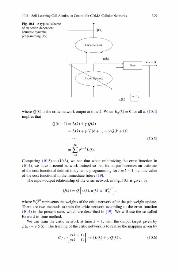
10.2 Self-Learning Call Admission Control for CDMA Cellular Networks 399
Fig. 10.1 A typical schemeof an action-dependentheuristic dynamicprogramming [19]
where Q(k) is the critic network output at time k. When Eq(k)= 0 for all k, (10.4)implies that
Q(k − 1)= L(k)+ γQ(k)
= L(k)+ γ [L(k + 1)+ γQ(k + 1)]= · · ·
=∞∑
i=k
γ i−kL(i).
(10.5)
Comparing (10.5) to (10.3), we see that when minimizing the error function in(10.4), we have a neural network trained so that its output becomes an estimateof the cost functional defined in dynamic programming for i = k + 1, i.e., the valueof the cost functional in the immediate future [19].
The input–output relationship of the critic network in Fig. 10.1 is given by
Q(k)=Q[x(k), u(k), k,W
(p)C
],
where W(p)C represents the weights of the critic network after the pth weight update.
There are two methods to train the critic network according to the error function(10.4) in the present case, which are described in [19]. We will use the so-calledforward-in-time method.
We can train the critic network at time k − 1, with the output target given byL(k)+ γQ(k). The training of the critic network is to realize the mapping given by
Cf :{x(k − 1)u(k − 1)
}→ {L(k)+ γQ(k)}. (10.6)
400 10 Other Applications of ADP
In this case, the output from the network to be trained is Q(k−1) and the input to thenetwork to be trained is composed of x(k− 1) and u(k− 1). The target output valuefor the critic network training is calculated using its output at time k as indicated in(10.6). The goal of learning the function given by (10.6) is to have the critic networkoutput satisfy
Q(k − 1)≈ L(k)+ γQ(k) for all k,
which is required by (10.5) for adaptive dynamic programming solutions.The critic network training procedure is described as follows using the strategy
of [16]:
1. Initialize two critic networks: cnet1 = cnet2;2. Use cnet2 to get Q(k), and then train cnet1 for 50 epochs using the Levenberg–
Marquardt algorithm [11];3. Copy cnet1 to cnet2, i.e., let cnet2 = cnet1;4. Repeat Steps 2 and 3, e.g., four times;5. Repeat Steps 1–4, e.g., ten times (start from different initial weights);6. Pick the best cnet1 obtained as the trained critic network.
After the critic network’s training is finished, the action network’s training startswith the objective of minimizing the critic network output Q(k). In this case, wecan choose the target of the action network training as zero, i.e., we will update theaction network’s weights so that the output of the critic network becomes as smallas possible. In general, a good critic network should not output negative values ifL(k) is non-negative. This is particularly true when L(k) is chosen as the squareerror function in tracking control problems [31]. The desired mapping which willbe used for the training of the action network in Fig. 10.1 is given by
A : {x(k)} → {0(k)}, (10.7)
where 0(k) indicates the target values of zero. We note that during the training ofthe action network, it will be connected to the critic network as shown in Fig. 10.1.The target in (10.7) is for the output of the whole network, i.e., the output of thecritic network after it is connected to the action network as shown in Fig. 10.1.
There are many problems in practice that have a control action space that is finite.Typical examples include bang-bang control applications where the control signalonly takes a few (finite) extreme values or vectors. When the application has only afinite action space, the decisions that can be made are constrained to a limited num-ber of choices, e.g., a binary choice in the case of call admission control problem.When a new call or a handoff call arrives at a base station requesting admission, thedecisions that a base station can make are constrained to two choices, i.e., to acceptthe call or to reject the call. Let us denote the two options by using u(k) = +1 for“accept” and u(k) = −1 for “reject”. It is important to realize that in the presentcase the control actions are limited to a binary choice, or to only two possible op-tions. Because of this, the ACDs introduced in Fig. 10.1 can be further simplified,so that only the critic network is needed. Our self-learning call admission control
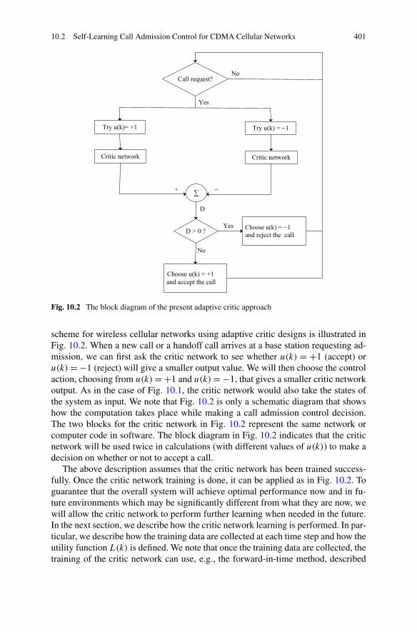
10.2 Self-Learning Call Admission Control for CDMA Cellular Networks 401
Fig. 10.2 The block diagram of the present adaptive critic approach
scheme for wireless cellular networks using adaptive critic designs is illustrated inFig. 10.2. When a new call or a handoff call arrives at a base station requesting ad-mission, we can first ask the critic network to see whether u(k) = +1 (accept) oru(k)= −1 (reject) will give a smaller output value. We will then choose the controlaction, choosing from u(k)= +1 and u(k)= −1, that gives a smaller critic networkoutput. As in the case of Fig. 10.1, the critic network would also take the states ofthe system as input. We note that Fig. 10.2 is only a schematic diagram that showshow the computation takes place while making a call admission control decision.The two blocks for the critic network in Fig. 10.2 represent the same network orcomputer code in software. The block diagram in Fig. 10.2 indicates that the criticnetwork will be used twice in calculations (with different values of u(k)) to make adecision on whether or not to accept a call.
The above description assumes that the critic network has been trained success-fully. Once the critic network training is done, it can be applied as in Fig. 10.2. Toguarantee that the overall system will achieve optimal performance now and in fu-ture environments which may be significantly different from what they are now, wewill allow the critic network to perform further learning when needed in the future.In the next section, we describe how the critic network learning is performed. In par-ticular, we describe how the training data are collected at each time step and how theutility function L(k) is defined. We note that once the training data are collected, thetraining of the critic network can use, e.g., the forward-in-time method, described
402 10 Other Applications of ADP
in this section. We also note that the description here for the critic network trainingapplies to both the initial training of the critic network and further training of thecritic network when needed in the future.
10.2.2.2 Self-learning Call Admission Control for CDMA Cellular Networks
We use a utility function as reward or penalty to the action made by the call ad-mission control scheme. When the call admission control scheme makes a decisionabout accepting a call, it will lead to two distinct results. The first is that the deci-sion of accepting a call is indeed the right decision due to the guarantee of qualityof service during the entire call duration. In this case we should give a reward tothe decision of accepting a call. Otherwise, a penalty is assigned to this decision.On the other hand, if rejecting a call would have been the right decision due tocall dropping or system outage after the call acceptance, we will also give a re-ward to the decision of rejecting a call. Otherwise, a penalty is assigned to thisdecision.
It is generally accepted in practice that handoff calls will be given higher prioritythan new calls [12, 26, 27, 29]. This is accomplished in our call admission con-trol scheme by using different thresholds for new calls and handoff calls. A hand-off call can be admitted if 0 < S∗
n ≤ Hσ(n) for all n = 0,1, . . . ,N . A new callcan only be admitted if 0 < S∗
0 ≤ Tσ(0) and 0 < S∗n ≤ Hσ(n) for n = 1,2, . . . ,N ,
where Tσ(0) < Hσ(0) is the threshold for new calls (where connection 0 is the newcaller).
For handoff calls, when 0 < S∗n ≤Hσ(n) for n= 0,1, . . . ,N , accepting a handoff
call will be given a reward and rejecting a handoff call will be given a penalty. Onthe other hand, when S∗
n > Hσ(n) for some n, 0 ≤ n ≤ N , accepting a handoff call(i.e., the zeroth caller) will be given a penalty and rejecting a handoff call will begiven a reward. Obviously, when S∗
n ≤ 0 for some n, 0 ≤ n≤N , the call should berejected. We note that if the power control algorithm leads to either S∗
n > Hσ(n) orS∗n ≤ 0 for some n, the network will enter an outage, i.e., some calls will have to be
terminated prematurely since they cannot maintain required quality of service (biterror rate). In this case, the action of rejection is given a reward and the action ofacceptance is given a penalty. Note that S∗
n , n = 0,1, . . . ,N , are power levels forall connections after the call admission decision and the power control algorithmconvergence.
We first define the cost functional for handoff calls as follows (S∗n ≥ 0 for n =
0,1, . . . ,N ):
En = ξ max
{u(k)
[S∗n
Hσ(n)
− 1
],0
}, (10.8)
where ξ > 0 is a coefficient, and u(k)= 1 represents accepting a call and u(k)= −1represents rejecting a call. We emphasize that the conditions, 0 ≤ S∗
n ≤ Hσ(n) forn= 0,1, . . . ,N , must hold for the entire duration of all calls in order for the systemto give reward to the action of accepting a handoff call.
10.2 Self-Learning Call Admission Control for CDMA Cellular Networks 403
For new calls, when 0 < S∗0 ≤ Tσ(0) and 0 < S∗
n ≤Hσ(n) for n= 1,2, . . . ,N , wegive a reward to the action of accepting a new call, and we give a penalty to theaction of rejecting a new call. When S∗
0 > Tσ(0), or S∗n > Hσ(n) for some n, n =
1,2, . . . ,N , or S∗n ≤ 0 for some n, n= 0,1, . . . ,N , we give penalty for accepting a
new call and we give a reward for rejecting a new call. The cost functional for newcalls is defined as (S∗
n ≥ 0 for n= 0,1, . . . ,N ):
En =
⎧⎪⎪⎪⎪⎨
⎪⎪⎪⎪⎩
ξ max
{[S∗n
Tσ(n)− 1
],0
}, when u(k)= 1,
ξ max
{[1 − S∗
n
Hσ(n)
],0
}, when u(k)= −1,
(10.9)
where Tσ(n) < Hσ(n), n= 0,1, . . . ,N . We note again that the conditions, 0 < S∗n ≤
Hσ(n) for n= 0,1, . . . ,N , must hold for the entire duration of all calls in order forthe system to give reward to the action of accepting a new call, even though theadmission decision is according to the condition 0 < S∗
0 ≤ Tσ(0) for the new call.The functions defined above satisfy the condition that En ≥ 0 for all n, n =
0,1, . . . ,N . From (10.8) and (10.9), we see that when the action is “accept”, if thevalue of the utility function of any connection is larger than 0, this action shouldbe penalized. Also, when the action is “reject”, if the value of the utility function ofany connection is zero, this action should be rewarded. Therefore, from the system’spoint of view, the cost function should be chosen as
E =⎧⎨
⎩
max0≤n≤N
(En), if u(k)= 1,
min0≤n≤N(En), if u(k)= −1.
(10.10)
The cost function defined in (10.10) indicates that the goal of our call admissioncontrol algorithm is to minimize the value of function E, i.e., to reach its minimumvalue of zero and to avoid its positive values.
The utility function L (used in (10.3)) in our present work is chosen as
L(u)= E
1 +E. (10.11)
Figures 10.3 and 10.4 show plots of this utility function for handoff calls and newcalls, respectively, when ξ = 10. The parameter ξ is used to obtain a desired shapeof the utility function. Since our algorithm will search for the optimal performancethat corresponds to small values of the utility function, the shape of the utility func-tion will have some effects on the optimization process. When ξ = 10, we see thatthe utility function becomes more selective than ξ = 1 for any condition indicatedby signal power. From Figs. 10.3 and 10.4 we see that the choice of the presentutility functions in (10.11) clearly shows minimum points (the flat areas) that our
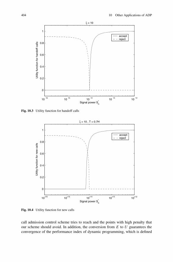
404 10 Other Applications of ADP
Fig. 10.3 Utility function for handoff calls
Fig. 10.4 Utility function for new calls
call admission control scheme tries to reach and the points with high penalty thatour scheme should avoid. In addition, the conversion from E to U guarantees theconvergence of the performance index of dynamic programming, which is defined
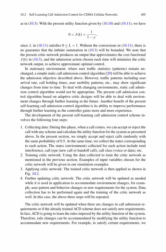
10.2 Self-Learning Call Admission Control for CDMA Cellular Networks 405
as in (10.3). With the present utility function given by (10.10) and (10.11), we have
0 < J(k) <1
1 − γ,
since L in (10.11) satisfies 0 ≤ L < 1. Without the conversions in (10.11), there isno guarantee that the infinite summation in (10.3) will be bounded. We note thatthe present critic network produces an output that approximates the cost functionalJ (k) in (10.3), and the admission action chosen each time will minimize the criticnetwork output, to achieve approximate optimal control.
In stationary environment, where user traffic statistics (patterns) remain un-changed, a simple static call admission control algorithm [20] will be able to achievethe admission objective described above. However, traffic patterns including userarrival rate, call holding times, user mobility patterns, etc., may show significantchanges from time to time. To deal with changing environments, static call admis-sion control algorithm would not be appropriate. The present call admission con-trol algorithm based on adaptive critic designs will be able to deal with environ-ment changes through further learning in the future. Another benefit of the presentself-learning call admission control algorithm is its ability to improve performancethrough further learning as the controller gains more and more experience.
The development of the present self-learning call admission control scheme in-volves the following four steps:
1. Collecting data: During this phase, when a call comes, we can accept or reject thecall with any scheme and calculate the utility function for the system as presentedabove. In the present section, we simply accept and reject calls randomly withthe same probability of 0.5. At the same time, we collect the states correspondingto each action. The states (environment) collected for each action include totalinterference, call type (new call or handoff call), call class (voice or data), etc.
2. Training critic network: Using the data collected to train the critic network asmentioned in the previous section. Examples of input variables chosen for thecritic network will be given in our simulation examples.
3. Applying critic network: The trained critic network is then applied as shown inFig. 10.2.
4. Further updating critic network: The critic network will be updated as neededwhile it is used in application to accommodate environment changes, for exam-ple, user pattern and behavior changes or new requirements for the system. Datacollection has to be performed again and the training of the critic network aswell. In this case, the above three steps will be repeated.
The critic network will be updated when there are changes in call admission re-quirements or if the already trained ACD scheme does not satisfy new requirements.In fact, ACD is going to learn the rules imposed by the utility function of the system.Therefore, rule changes can be accommodated by modifying the utility function toaccommodate new requirements. For example, to satisfy certain requirements, we
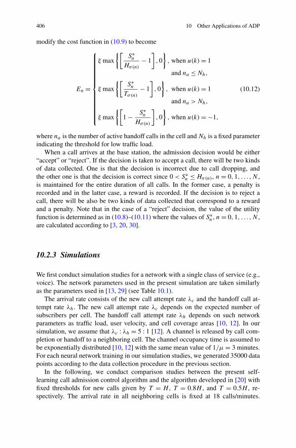
406 10 Other Applications of ADP
modify the cost function in (10.9) to become
En =
⎧⎪⎪⎪⎪⎪⎪⎪⎪⎪⎪⎪⎪⎨
⎪⎪⎪⎪⎪⎪⎪⎪⎪⎪⎪⎪⎩
ξ max
{[S∗n
Hσ(n)
− 1
],0
}, when u(k)= 1
and na ≤Nh,
ξ max
{[S∗n
Tσ(n)− 1
],0
}, when u(k)= 1
and na > Nh,
ξ max
{[1 − S∗
n
Hσ(n)
],0
}, when u(k)= −1,
(10.12)
where na is the number of active handoff calls in the cell and Nh is a fixed parameterindicating the threshold for low traffic load.
When a call arrives at the base station, the admission decision would be either“accept” or “reject”. If the decision is taken to accept a call, there will be two kindsof data collected. One is that the decision is incorrect due to call dropping, andthe other one is that the decision is correct since 0 < S∗
n ≤ Hσ(n), n = 0,1, . . . ,N ,is maintained for the entire duration of all calls. In the former case, a penalty isrecorded and in the latter case, a reward is recorded. If the decision is to reject acall, there will be also be two kinds of data collected that correspond to a rewardand a penalty. Note that in the case of a “reject” decision, the value of the utilityfunction is determined as in (10.8)–(10.11) where the values of S∗
n , n= 0,1, . . . ,N ,are calculated according to [3, 20, 30].
10.2.3 Simulations
We first conduct simulation studies for a network with a single class of service (e.g.,voice). The network parameters used in the present simulation are taken similarlyas the parameters used in [13, 29] (see Table 10.1).
The arrival rate consists of the new call attempt rate λc and the handoff call at-tempt rate λh. The new call attempt rate λc depends on the expected number ofsubscribers per cell. The handoff call attempt rate λh depends on such networkparameters as traffic load, user velocity, and cell coverage areas [10, 12]. In oursimulation, we assume that λc : λh = 5 : 1 [12]. A channel is released by call com-pletion or handoff to a neighboring cell. The channel occupancy time is assumed tobe exponentially distributed [10, 12] with the same mean value of 1/μ= 3 minutes.For each neural network training in our simulation studies, we generated 35000 datapoints according to the data collection procedure in the previous section.
In the following, we conduct comparison studies between the present self-learning call admission control algorithm and the algorithm developed in [20] withfixed thresholds for new calls given by T = H , T = 0.8H , and T = 0.5H , re-spectively. The arrival rate in all neighboring cells is fixed at 18 calls/minutes.
10.2 Self-Learning Call Admission Control for CDMA Cellular Networks 407
Table 10.1 Networkparameters Parameters Values Parameters Values
W 1.2288 Mcps R 9.6 kbps
η 1 × 10⁻¹⁴ W H 1 × 10⁻¹⁴ W
Eb/N0 7 dB v 3/8
Fig. 10.5 Comparison study using utility function defined in (10.9)
The training data are collected as mentioned in the previous section. We chooseTσ(n) = 0.5Hσ(n) and ξ = 10 in (10.9). The critic network has three inputs. The firstis the total interference received at the base station, the second is the action (1 foraccepting, −1 for rejecting), and the third is the call type (1 for new calls, −1 forhandoff calls). The critic network is a multilayer feedforward neural network with3–6–1 structure, i.e., three neurons at the input layer, six neurons at the hidden layer,and one neuron at the output layer. Both the hidden and the output layers use thehyperbolic tangent function as the activation function. Figure 10.5 shows the simu-lation results. We see from the figure that the performance of the self-learning algo-rithm is similar to the case of static algorithm with T = 0.5H , because we chooseTσ(n) = 0.5Hσ(n) in (10.9) for our learning control algorithm. When the call arrivalrate is low, the self-learning algorithm is not so good because it reserves too muchfor handoff calls and as a result it rejects too many new calls. That is why the GoSis worse than the other two cases of static algorithms (T = 1.0H and T = 0.8H ).In this case, the self-learning algorithm is trained to learn a call admission controlscheme that gives higher priority to handoff calls.
408 10 Other Applications of ADP
Fig. 10.6 Comparison study using utility function defined in (10.12)
In order to improve the GoS when the call arrival rate is low, we use the mod-ified cost function for new calls as in (10.12), where we choose Nh = 15 in oursimulation. Using this new utility function we collect the training data using one ofthe static algorithms with fixed threshold or the previous critic network. Then wetrain a new critic network with the newly collected data. In this time the critic net-work has four inputs. Three of them are the same as in the previous critic network.The new input is equal to 1 when na ≤ Nh and otherwise it is equal to −1. Thecritic network in this case has a structure given by 4–8–1. Figure 10.6 shows theresult of applying the new critic network to the same traffic pattern as in Fig. 10.5.From the figure we see that the self-learning algorithm using the new critic networkhas the best GoS. We see that by simply changing the cost function from (10.11)to (10.12), the self-learning algorithm can significantly improve its performance tooutperform static admission control algorithms. One of the benefits of self-learningcall admission control algorithm is that we can easily and efficiently design call ad-mission control algorithms by modifying the cost function (equivalently, the utilityfunction) to satisfy the requirements or to accommodate new environment changes.
The traffic load in telephony systems is typically time varying. Figure 10.7 showsa pattern concerning call arrivals during a typical 24 hour business day, beginning atmidnight [8]. It can be seen that the peak hours occur around 11:00 am and 4:00 pm.Next, we use our newly trained critic network above for this traffic pattern. Fig-ure 10.8 gives the simulation results under the assumption that the traffic load wasspatially uniformly distributed among cells, but followed the time-varying patterngiven in Fig. 10.7. Figure 10.8 compares the four call admission control algorithmsand shows that the self-learning algorithm has the best GoS among all the algo-rithms tested. We note that the self-learning call admission control algorithm was
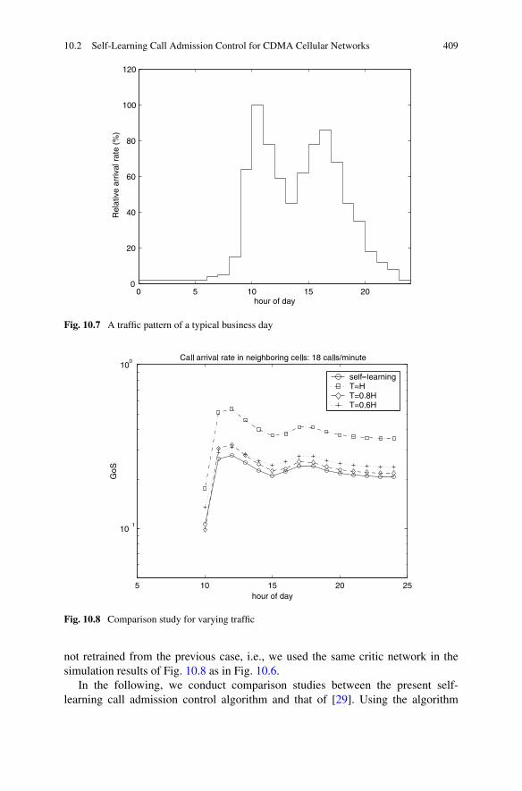
10.2 Self-Learning Call Admission Control for CDMA Cellular Networks 409
Fig. 10.7 A traffic pattern of a typical business day
Fig. 10.8 Comparison study for varying traffic
not retrained from the previous case, i.e., we used the same critic network in thesimulation results of Fig. 10.8 as in Fig. 10.6.
In the following, we conduct comparison studies between the present self-learning call admission control algorithm and that of [29]. Using the algorithm
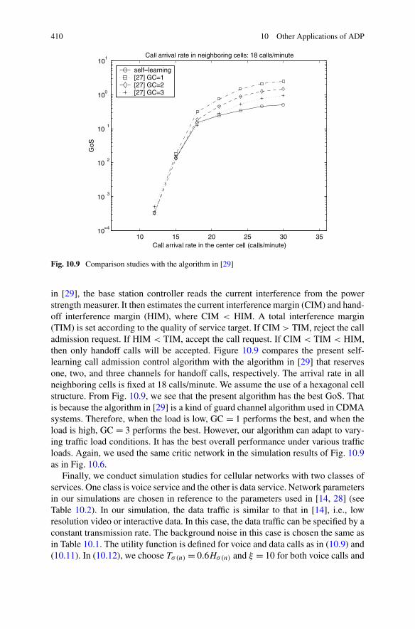
410 10 Other Applications of ADP
Fig. 10.9 Comparison studies with the algorithm in [29]
in [29], the base station controller reads the current interference from the powerstrength measurer. It then estimates the current interference margin (CIM) and hand-off interference margin (HIM), where CIM < HIM. A total interference margin(TIM) is set according to the quality of service target. If CIM > TIM, reject the calladmission request. If HIM < TIM, accept the call request. If CIM < TIM < HIM,then only handoff calls will be accepted. Figure 10.9 compares the present self-learning call admission control algorithm with the algorithm in [29] that reservesone, two, and three channels for handoff calls, respectively. The arrival rate in allneighboring cells is fixed at 18 calls/minute. We assume the use of a hexagonal cellstructure. From Fig. 10.9, we see that the present algorithm has the best GoS. Thatis because the algorithm in [29] is a kind of guard channel algorithm used in CDMAsystems. Therefore, when the load is low, GC = 1 performs the best, and when theload is high, GC = 3 performs the best. However, our algorithm can adapt to vary-ing traffic load conditions. It has the best overall performance under various trafficloads. Again, we used the same critic network in the simulation results of Fig. 10.9as in Fig. 10.6.
Finally, we conduct simulation studies for cellular networks with two classes ofservices. One class is voice service and the other is data service. Network parametersin our simulations are chosen in reference to the parameters used in [14, 28] (seeTable 10.2). In our simulation, the data traffic is similar to that in [14], i.e., lowresolution video or interactive data. In this case, the data traffic can be specified by aconstant transmission rate. The background noise in this case is chosen the same asin Table 10.1. The utility function is defined for voice and data calls as in (10.9) and(10.11). In (10.12), we choose Tσ(n) = 0.6Hσ(n) and ξ = 10 for both voice calls and
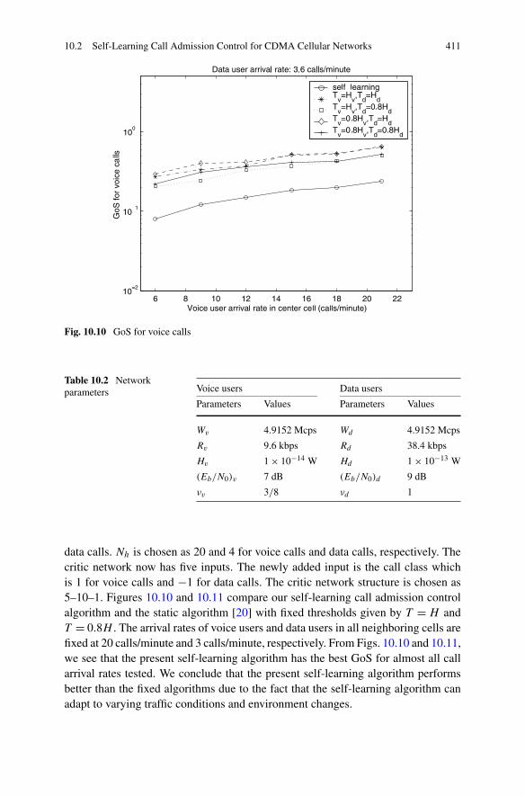
10.2 Self-Learning Call Admission Control for CDMA Cellular Networks 411
Fig. 10.10 GoS for voice calls
Table 10.2 Networkparameters Voice users Data users
Parameters Values Parameters Values
Wv 4.9152 Mcps Wd 4.9152 Mcps
Rv 9.6 kbps Rd 38.4 kbps
Hv 1 × 10⁻¹⁴ W Hd 1 × 10⁻¹³ W
(Eb/N0)v 7 dB (Eb/N0)d 9 dB
νv 3/8 νd 1
data calls. Nh is chosen as 20 and 4 for voice calls and data calls, respectively. Thecritic network now has five inputs. The newly added input is the call class whichis 1 for voice calls and −1 for data calls. The critic network structure is chosen as5–10–1. Figures 10.10 and 10.11 compare our self-learning call admission controlalgorithm and the static algorithm [20] with fixed thresholds given by T = H andT = 0.8H . The arrival rates of voice users and data users in all neighboring cells arefixed at 20 calls/minute and 3 calls/minute, respectively. From Figs. 10.10 and 10.11,we see that the present self-learning algorithm has the best GoS for almost all callarrival rates tested. We conclude that the present self-learning algorithm performsbetter than the fixed algorithms due to the fact that the self-learning algorithm canadapt to varying traffic conditions and environment changes.
412 10 Other Applications of ADP
Fig. 10.11 GoS for data calls
10.3 Engine Torque and Air–Fuel Ratio Control Based on ADP
10.3.1 Problem Formulation
A test vehicle with a V8 engine and 4-speed automatic transmission is instrumentedwith engine and transmission torque sensors, wide-range air–fuel ratio sensors in theexhaust pipe located before and after the catalyst on each bank, as well as exhaustgas pressure and temperature sensors. The vehicle is also equipped with a dSPACErapid prototyping controller for data collection and controller implementation. Dataare collected at each engine event under various driving conditions, such as theFederal Test Procedure (FTP cycles), as well as more aggressive driving patterns, fora length of about 95,000 samples during each test. The engine is run under closed-loop fuel control using switching-type oxygen sensors. The dSPACE is interfacedwith the power-train control module (PCM) in a by-pass mode.
We build a neural network model for the test engine with a structure compatiblewith the mathematical engine model developed by Dobner [5, 6, 22] and others. Dueto the complexity of modern automotive engines, in the present work, we use thetime-lagged recurrent neural networks (TLRNs) for engine modeling. In practice,TLRNs have been used often for function approximation and it is believed that theyare more powerful than the networks with only feedforward structures (cf. [25, 33]).
For the neural network engine model, we choose air–fuel ratio (AFR) and enginetorque (TRQ) as the two outputs. We choose throttle position (TPS), electrical fuelpulse width (FPW), and spark advance (SPA) as the three control inputs. These are
10.3 Engine Torque and Air–Fuel Ratio Control Based on ADP 413
input signals to be generated using our new adaptive critic learning control algo-rithm. We choose intake manifold pressure (MAP), mass air flow rate (MAF), andengine speed (RPM) as reference input. The time-lagged recurrent neural networkused for the engine combustion module has six input neurons, a single hidden layerwith eight neurons, and two output neurons.
Validation results for the output TRQ and AFR of the neural network enginemodel indicate a very good match between the real vehicle data and the neural net-work model output during the validation phase [15].
10.3.2 Self-learning Neural Network Control for Both EngineTorque and Exhaust Air–Fuel Ratio
Suppose that one is given a discrete-time non-linear dynamical system
x(k + 1)= F [x(k), u(k), k], (10.13)
where x ∈ Rn represents the state vector of the system and u ∈ R
m denotes thecontrol action. Suppose that one associates with this system the cost functional (orcost)
J [x(i), i] =∞∑
k=i
γ k−iL[x(k), u(k), k], (10.14)
where L is called the utility function or local cost function and γ is the discountfactor with 0 < γ ≤ 1. Note that J is dependent on the initial time i and the initialstate x(i), and it is referred to as the cost-to-go of state x(i). The objective is tochoose the control sequence u(k), k = i, i + 1, . . . , so that the cost functional J(i.e., the cost) in (10.14) is minimized.
Adaptive critic designs (ACDs) are defined as designs that approximate dy-namic programming in the general case, i.e., approximate optimal control overtime in noisy, non-linear environments. A typical design of ACDs consists of threemodules—Critic (for evaluation), Model (for prediction), and Action (for deci-sion). When in ACDs the critic network (i.e., the evaluation module) takes the ac-tion/control signal as part of its input, the designs are referred to as action-dependentACDs (ADACDs). We use an action-dependent version of ACDs that does not re-quire the explicit use of the model network in the design. The critic network in thiscase will be trained by minimizing the following error measure over time:
‖Eq‖ =∑
k
Eq(k)
=∑
k
[Q(k − 1)−L(k)− γQ(k)
]2,
(10.15)
414 10 Other Applications of ADP
where Q(k)=Q[x(k), u(k), k,WC]. When Eq(k)= 0 for all k, (10.15) implies that
Q(k − 1)= L(k)+ γQ(k)
= L(k)+ γ [L(k + 1)+ γQ(k + 1)]= · · ·
=∞∑
i=k
γ i−kL(k).
(10.16)
We see that when minimizing the error function in (10.15), we have a neural networktrained so that its output at time k becomes an estimate of the cost functional definedin dynamic programming for i = k + 1, i.e., the value of the cost functional in theimmediate future [19].
The input–output relationship of the critic network is given by
Q(k)=Q [x(k), u(k), k,WC] ,
where WC represents the weight vector of the critic network.We can train the critic network at time k− 1, with the desired output target given
by L(k)+ γQ(k). The training of the critic network is to realize the mapping givenby
Cf :{x(k − 1)u(k − 1)
}→ {L(k)+ γQ(k)}. (10.17)
We consider Q(k − 1) in (10.15) as the output from the network to be trained andthe target output value for the critic network is calculated using its output at time k.
After the critic network’s training is finished, the action network’s training startswith the objective of minimizing Q(k). The goal of the action network training isto minimize the critic network output Q(k). In this case, we can choose the targetof the action network training as zero, i.e., we will train the action network so thatthe output of the critic network becomes as small as possible. The desired mappingwhich will be used for the training of the action network in the present ADHDP isgiven by
A : {x(k)} → {0(k)}, (10.18)
where 0(k) indicates the target values of zero. We note that during the training ofthe action network, it will be connected to the critic network to form a larger neuralnetwork. The target in (10.18) is for the output of the whole network, i.e., the outputof the critic network after it is connected to the action network.
After the action network’s training cycle is completed, one may check the sys-tem’s performance, then stop or continue the training procedure by going back tothe critic network’s training cycle again, if the performance is not acceptable yet.
10.3 Engine Torque and Air–Fuel Ratio Control Based on ADP 415
Assume that the control objective is to have x(k) in (10.13) track another signalgiven by x∗(k). We define in this case the local cost function L(k) as
L(k)= 1
2eT(k)e(k)= 1
2[x(k)− x∗(k)]T[x(k)− x∗(k)].
Using the ADHDP introduced earlier in this section, we can design a controller tominimize
J (k)=∞∑
i=k
γ i−kL(i),
where 0 < γ < 1. We note that in this case our control objective is to minimizean infinite summation of L(k) from the current time to the infinite future, while inconventional tracking control designs, the objective is often to minimize L(k) itself.
10.3.3 Simulations
The objective of the present engine controller design is to provide control signalsso that the torque generated by the engine will track the torque measurement asin the data and the air–fuel ratio will track the required values also as in the data.The measured torque values in the data are generated by the engine using the exist-ing controller. Our learning controller will assume no knowledge about the controlsignals provided by the existing controller. It will generate a set of control signalsthat are independent of the control signals in the measured data. Based on the datacollected, we use our learning controller to generate control signals TPS, FPW, andSPA, with the goal of producing exactly the same torque and air–fuel ratio as in thedata set. That is to say, we keep our system under the same requirements as the datacollected, and we build a controller that provides control signals which achieve thetorque control and air–fuel ratio control performance of the engine.
As described in the previous section, the development of an adaptive critic learn-ing controller involves two stages: the training of a critic network and the develop-ment of a controller/action network. We describe in the rest of the present sectionthe learning control design for tracking the TRQ and AFR measurements in the dataset. This is effectively a torque-based controller, i.e., a controller that can generatecontrol signals given the torque demand. The block diagram of the present adaptivecritic engine control (including air–fuel ratio control) is shown in Fig. 10.12. Thediagram shows how adaptive critic designs can be applied to engine control throughadaptive dynamic programming.
10.3.3.1 Critic Network
The critic network is chosen as a 8–15–1 structure with eight input neurons and 15hidden layer neurons:
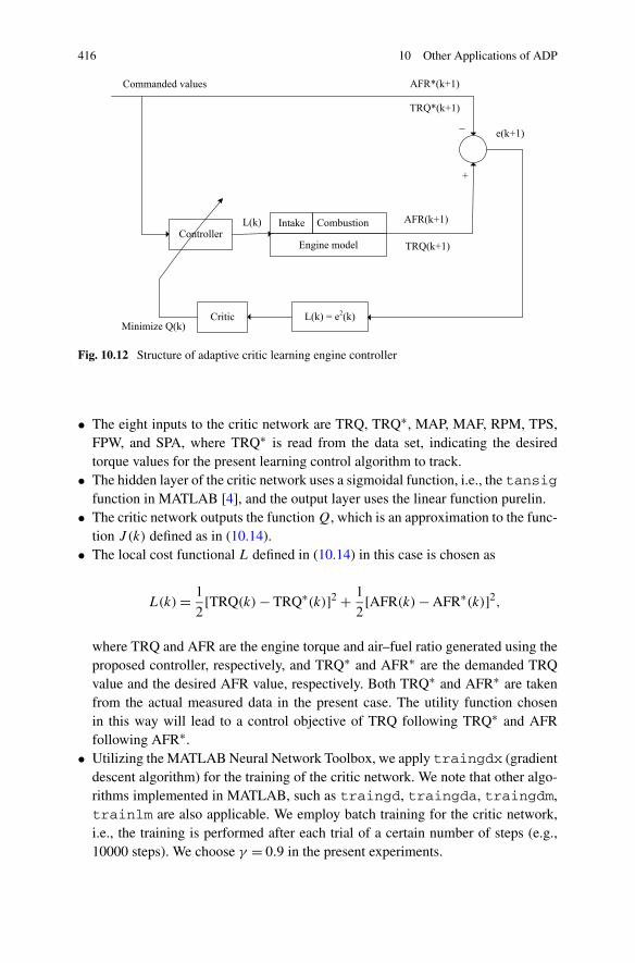
416 10 Other Applications of ADP
Fig. 10.12 Structure of adaptive critic learning engine controller
• The eight inputs to the critic network are TRQ, TRQ∗, MAP, MAF, RPM, TPS,FPW, and SPA, where TRQ∗ is read from the data set, indicating the desiredtorque values for the present learning control algorithm to track.
• The hidden layer of the critic network uses a sigmoidal function, i.e., the tansigfunction in MATLAB [4], and the output layer uses the linear function purelin.
• The critic network outputs the function Q, which is an approximation to the func-tion J (k) defined as in (10.14).
• The local cost functional L defined in (10.14) in this case is chosen as
L(k)= 1
2[TRQ(k)− TRQ∗(k)]2 + 1
2[AFR(k)− AFR∗(k)]2,
where TRQ and AFR are the engine torque and air–fuel ratio generated using theproposed controller, respectively, and TRQ∗ and AFR∗ are the demanded TRQvalue and the desired AFR value, respectively. Both TRQ∗ and AFR∗ are takenfrom the actual measured data in the present case. The utility function chosenin this way will lead to a control objective of TRQ following TRQ∗ and AFRfollowing AFR∗.
• Utilizing the MATLAB Neural Network Toolbox, we apply traingdx (gradientdescent algorithm) for the training of the critic network. We note that other algo-rithms implemented in MATLAB, such as traingd, traingda, traingdm,trainlm are also applicable. We employ batch training for the critic network,i.e., the training is performed after each trial of a certain number of steps (e.g.,10000 steps). We choose γ = 0.9 in the present experiments.
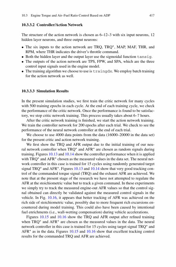
10.3 Engine Torque and Air–Fuel Ratio Control Based on ADP 417
10.3.3.2 Controller/Action Network
The structure of the action network is chosen as 6–12–3 with six input neurons, 12hidden layer neurons, and three output neurons:
• The six inputs to the action network are TRQ, TRQ∗, MAP, MAF, THR, andRPM, where THR indicates the driver’s throttle command.
• Both the hidden layer and the output layer use the sigmoidal function tansig.• The outputs of the action network are TPS, FPW, and SPA, which are the three
control input signals used in the engine model.• The training algorithm we choose to use is traingdx. We employ batch training
for the action network as well.
10.3.3.3 Simulation Results
In the present simulation studies, we first train the critic network for many cycleswith 500 training epochs in each cycle. At the end of each training cycle, we checkthe performance of the critic network. Once the performance is found to be satisfac-tory, we stop critic network training. This process usually takes about 6–7 hours.
After the critic network training is finished, we start the action network training.We train the controller network for 200 epochs after each trial. We check to see theperformance of the neural network controller at the end of each trial.
We choose to use 4000 data points from the data (16000–20000 in the data set)for the present critic and action network training.
We first show the TRQ and AFR output due to the initial training of our neu-ral network controller when TRQ∗ and AFR∗ are chosen as random signals duringtraining. Figures 10.13 and 10.14 show the controller performance when it is appliedwith TRQ∗ and AFR∗ chosen as the measured values in the data set. The neural net-work controller in this case is trained for 15 cycles using randomly generated targetsignal TRQ∗ and AFR∗. Figures 10.13 and 10.14 show that very good tracking con-trol of the commanded torque signal (TRQ) and the exhaust AFR are achieved. Wenote that at the present stage of the research we have not attempted to regulate theAFR at the stoichiometric value but to track a given command. In these experimentswe simply try to track the measured engine-out AFR values so that the control sig-nal obtained can directly be validated against the measured control signals in thevehicle. In Fig. 10.16, it appears that better tracking of AFR was achieved on therich side of stoichiometric value, possibly due to more frequent rich excursions en-countered during model training. This could also have been caused by intentionalfuel enrichments (i.e., wall-wetting compensation) during vehicle accelerations.
Figures 10.15 and 10.16 show the TRQ and AFR output after refined trainingwhen TRQ∗ and AFR∗ are chosen as the measured values in the data. The neuralnetwork controller in this case is trained for 15 cycles using target signal TRQ∗ andAFR∗ as in the data. Figures 10.15 and 10.16 show that excellent tracking controlresults for the commanded TRQ and AFR are achieved.
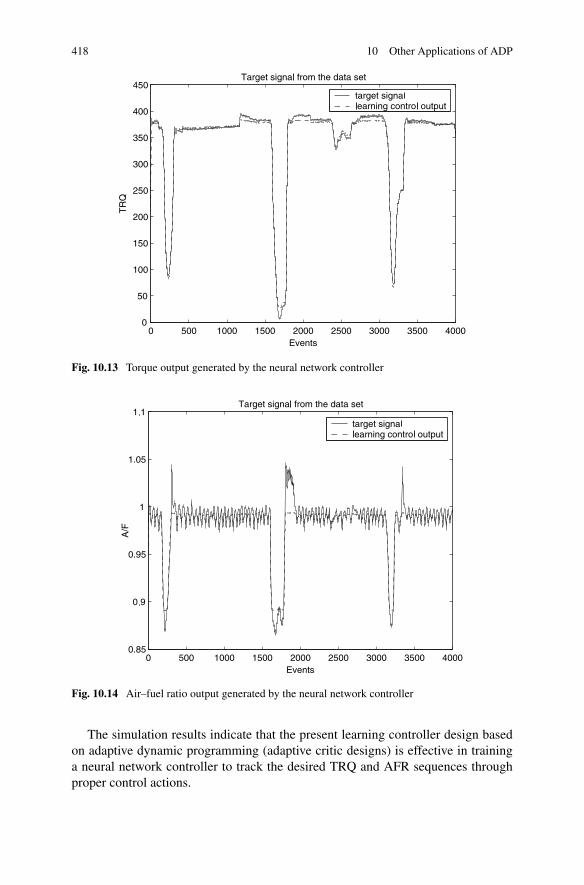
418 10 Other Applications of ADP
Fig. 10.13 Torque output generated by the neural network controller
Fig. 10.14 Air–fuel ratio output generated by the neural network controller
The simulation results indicate that the present learning controller design basedon adaptive dynamic programming (adaptive critic designs) is effective in traininga neural network controller to track the desired TRQ and AFR sequences throughproper control actions.
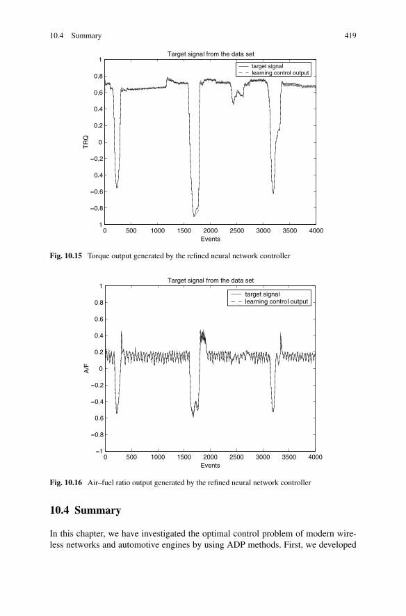
10.4 Summary 419
Fig. 10.15 Torque output generated by the refined neural network controller
Fig. 10.16 Air–fuel ratio output generated by the refined neural network controller
10.4 Summary
In this chapter, we have investigated the optimal control problem of modern wire-less networks and automotive engines by using ADP methods. First, we developed
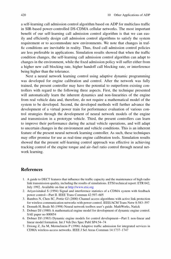
420 10 Other Applications of ADP
a self-learning call admission control algorithm based on ADP for multiclass trafficin SIR-based power-controlled DS-CDMA cellular networks. The most importantbenefit of our self-learning call admission control algorithm is that we can eas-ily and efficiently design call admission control algorithms to satisfy the systemrequirement or to accommodate new environments. We note that changes in traf-fic conditions are inevitable in reality. Thus, fixed call admission control policiesare less preferable in applications. Simulation results showed that when the trafficcondition changes, the self-learning call admission control algorithm can adapt tochanges in the environment, while the fixed admission policy will suffer either froma higher new call blocking rate, higher handoff call blocking rate, or interferencebeing higher than the tolerance.
Next a neural network learning control using adaptive dynamic programmingwas developed for engine calibration and control. After the network was fullytrained, the present controller may have the potential to outperform existing con-trollers with regard to the following three aspects. First, the technique presentedwill automatically learn the inherent dynamics and non-linearities of the enginefrom real vehicle data and, therefore, do not require a mathematical model of thesystem to be developed. Second, the developed methods will further advance thedevelopment of a virtual power train for performance evaluation of various con-trol strategies through the development of neural network models of the engineand transmission in a prototype vehicle. Third, the present controllers can learnto improve their performance during the actual vehicle operations, and will adaptto uncertain changes in the environment and vehicle conditions. This is an inherentfeature of the present neural network learning controller. As such, these techniquesmay offer promise for use as real-time engine calibration tools. Simulation resultsshowed that the present self-learning control approach was effective in achievingtracking control of the engine torque and air–fuel ratio control through neural net-work learning.
References
1. A guide to DECT features that influence the traffic capacity and the maintenance of high radiolink transmission quality, including the results of simulations. ETSI technical report: ETR 042,July 1992. Available on-line at http://www.etsi.org
2. Ariyavisitakul S (1994) Signal and interference statistics of a CDMA system with feedbackpower control—Part II. IEEE Trans Commun 42:597–605
3. Bambos N, Chen SC, Pottie GJ (2000) Channel access algorithms with active link protectionfor wireless communication networks with power control. IEEE/ACM Trans Netw 8:583–597
4. Demuth H, Beale M (1998) Neural network toolbox user’s guide. MathWorks, Natick5. Dobner DJ (1980) A mathematical engine model for development of dynamic engine control.
SAE paper no 8000546. Dobner DJ (1983) Dynamic engine models for control development—Part I: non-linear and
linear model formation. Int J Veh Des Spec Publ SP4:54–747. Dziong Z, Jia M, Mermelstein P (1996) Adaptive traffic admission for integrated services in
CDMA wireless-access networks. IEEE J Sel Areas Commun 14:1737–1747
References 421
8. Freeman RL (1996) Telecommunication system engineering. Wiley, New York9. Gilhousen KS, Jacobs IM, Padovani R, Viterbi AJ, Weaver LA, Wheatley CE III (1991) On
the capacity of a cellular CDMA system. IEEE Trans Veh Technol 40:303–31210. Guerin RA (1987) Channel occupancy time distribution in a cellular radio system. IEEE Trans
Veh Technol 35:89–9911. Hagan MT, Menhaj MB (1994) Training feedforward networks with the Marquardt algorithm.
IEEE Trans Neural Netw 5:989–99312. Hong D, Rappaport SS (1986) Traffic model and performance analysis for cellular mobile
radio telephone systems with prioritized and nonprioritized handoff procedures. IEEE TransVeh Technol 35:77–92
13. Kim DK, Sung DK (2000) Capacity estimation for an SIR-based power-controlled CDMAsystem supporting ON–OFF traffic. IEEE Trans Veh Technol 49:1094–1100
14. Kim YW, Kim DK, Kim JH, Shin SM, Sung DK (2001) Radio resource management inmultiple-chip-rate DS/CDMA systems supporting multiclass services. IEEE Trans Veh Tech-nol 50:723–736
15. Kovalenko O, Liu D, Javaherian H (2001) Neural network modeling and adaptive critic controlof automotive fuel-injection systems. In: Proceedings of IEEE international symposium onintelligent control, Taipei, Taiwan, pp 368–373
16. Lendaris GG, Paintz C (1997) Training strategies for critic and action neural networks indual heuristic programming method. In: Proceedings of international conference on neuralnetworks, Houston, TX, pp 712–717
17. Liu Z, Zarki ME (1994) SIR-based call admission control for DS-CDMA cellular systems.IEEE J Sel Areas Commun 12:638–644
18. Liu D, Zhang Y (2002) A new learning control approach suitable for problems with finiteaction space. In: Proceedings of international conference on control and automation, Xiamen,China, pp 1669–1673
19. Liu D, Xiong X, Zhang Y (2001) Action-dependent adaptive critic designs. In: Proceedings ofINNS-IEEE international joint conference on neural networks, Washington, DC, pp 990–995
20. Liu D, Zhang Y, Hu S (2004) Call admission policies based on calculated power controlsetpoints in SIR-based power-controlled DS-CDMA cellular networks. Wirel Netw 10:473–483
21. Liu D, Zhang Y, Zhang H (2005) A self-learning call admission control scheme for CDMAcellular networks. IEEE Transactions on Neural Networks 16:1219–1228
22. Liu D, Hu S, Zhang HG (2006) Simultaneous blind separation of instantaneous mixtures witharbitrary rank. IEEE Trans Circuits Syst I, Regul Pap 53:2287–2298
23. Liu D, Xiong X, DasGupta B, Zhang HG (2006) Motif discoveries in unaligned molecularsequences using self-organizing neural networks. IEEE Trans Neural Netw 17:919–928
24. Liu D, Javaherian H, Kovalenko O (2008) Adaptive critic learning techniques for enginetorque and air–fuel ratio control. IEEE Trans Syst Man Cybern, Part B, Cybern 38:988–993
25. Puskorius GV, Feldkamp LA, Davis LL (1996) Dynamic neural network methods applied toon-vehicle idle speed control. Proc IEEE 84:1407–1420
26. Ramjee R, Towsley D, Nagarajan R (1997) On optimal call admission control in cellular net-works. Wirel Netw 3:29–41
27. Rappaport SS, Purzynski C (1996) Prioritized resource assignment for mobile cellular com-munication systems with mixed services and platform types. IEEE Trans Veh Technol 45:443–458
28. Sampath A, Holtzman JM (1997) Access control of data in integrated voice/data CDMA sys-tems: benefits and tradeoffs. IEEE J Sel Areas Commun 15:1511–1526
29. Shin SM, Cho CH, Sung DK (1999) Interference-based channel assignment for DS-CDMAcellular systems. IEEE Trans Veh Technol 48:233–239
30. Veeravalli VV, Sendonaris A (1999) The coverage-capacity tradeoff in cellular CDMA sys-tems. IEEE Trans Veh Technol 48:1443–1450
422 10 Other Applications of ADP
31. Visnevski NA, Prokhorov DV (1996) Control of a nonlinear multivariable system with adap-tive critic designs. In: Proceedings of conference on artificial neural networks in engineering,St Louis, MO, pp 559–565
32. Viterbi AJ, Viterbi AM, Zehavi E (1994) Other-cell interference in cellular power-controlledCDMA. IEEE Trans Commun 42:1501–1504
33. Werbos PJ, McAvoy T, Su T (1992) Neural networks, system identification, and control in thechemical process industries. In: White DA, Sofge DA (eds) Handbook of intelligent control:neural, fuzzy, and adaptive approaches, Van Nostrand Reinhold, New York, NY
Index
Symbols2-D, 343
AAdaptive critic designs, 3, 6–8, 395, 398, 401,
405, 413, 415, 418Adaptive critic learning, 9, 413, 415Admissible control law, 14, 28, 33–35, 59, 60,
62, 63, 183, 229, 262, 263, 295Approximate dynamic programming, 3, 4, 17
BBackward iteration, 201, 207Bellman’s optimality principle, 53, 129, 143,
162, 170, 189, 290Boundary conditions, 310, 311, 328, 329
CCDMA, 396, 398, 410Cellular networks, 395–397, 401, 410, 420Composite control, 283, 288Curse of dimensionality, 3
DData-based, 223–226, 236, 238, 254, 309, 325,
332, 339–341, 343Delay matrix function, 161, 164, 166, 168,
172, 173, 197Descriptor system, 257, 271, 272, 306Dimension augmentation, 128Dynamic programming, 1–3, 259, 261, 311,
312, 333, 396, 399, 404, 414
FFixed terminal state, 83
GGARE, 17, 334, 341Gaussian density function, 39GHJB, 9, 10, 27, 71–73, 75, 76, 79
HHamilton function, 13, 14, 228–230, 312–315,
318, 323, 326, 374, 378, 379Hermitian, 203HJB, 3, 9, 10, 13, 16, 27–30, 35, 36, 39, 54,
71–73, 76, 80, 83, 85, 86, 113, 116,129, 131, 143, 144, 149, 161–164, 180,186, 189, 192, 201, 205, 210, 211, 213,257, 278, 279, 282–284, 286, 291, 296,297, 348, 355
HJI, 10, 309, 349
IInfinite-dimensional, 16, 163Initially stable policy, 10, 12
KKronecker, 17, 324, 325, 327, 340
LLagrange multiplier, 313Least-square method, 78, 203, 324, 325Lebesgue integral, 77Lower value function, 18, 346, 349, 354LQR, 13, 259Lyapunov function, 4, 13, 55, 56, 74, 213, 226,
232, 235, 247, 285, 351, 375, 381
MMixed optimal solution, 19, 345, 347, 348, 354Mixed optimal value function, 19, 346–348,
355, 358Monte Carlo, 3
H. Zhang et al., Adaptive Dynamic Programming for Control,Communications and Control Engineering, DOI 10.1007/978-1-4471-4757-2,© Springer-Verlag London 2013
423
424 Index
NNon-zero-sum, 345, 372–374, 378, 381, 390Nonquadratic functional, 27, 31, 72, 273, 291,
292, 305
OOptimal robust controller, 236, 237Oscillate, 111, 119
PPartial differential equation, 3Persistent excitation condition, 231, 379, 384Pseudocontrol, 243
QQuadratic polynomial, 324
RRBFNN, 39Recurrent neural network, 15, 223, 225, 412,
413Redundant weight, 268Regression function, 135Reinforcement learning, 3, 10, 11Robbins–Monro, 135, 136Roesser, 309, 310, 343
SSelf-learning, 395, 397, 398, 400, 405, 407,
408, 411, 420
Singularly perturbed system, 257, 281, 287,288, 306
SNAC, 8, 9, 257, 297Stabilization control, viSteady-state stage, 125–127, 228Switched system, 257–259, 262, 265, 270, 306
TTime delays, 16, 17, 161, 162, 197, 201, 202,
204, 207, 220Time-varying, 128, 358, 362–364, 408Transient stage, 125, 228TSADP, 257, 262, 263, 265, 268
UUpper value function, 18, 346, 349, 350,
352–354, 356Utility function, 1, 13, 18, 52, 82, 102, 142,
162, 179, 224, 228, 310, 332, 352,354–357, 395, 398, 401–403
WWC , 5While the input of the model network is x(k)
and vi (x(k)), 64
ZZero-sum games, 17, 19, 309, 311, 312, 314,
331–334, 339, 343, 345, 358, 361, 363,364, 370, 371, 392


![Aho Ullmann The Design And Analysis of Computer … Science/2_Algorithms/The... · BIBLIOGRAPHIC NOTES Cooley, Lewis, and Welch [1967] trace the origins of the fast Fourier transform](https://img.pdfslide.us/doc/110x75/5ac4d6037f8b9a5c558d065f/aho-ullmann-the-design-and-analysis-of-computer-science2algorithmsthebibliographic.jpg)