Embed Size (px)
Citation preview

EEccoonnoomm iiccss PPrrooggrraamm WWoorrkkiinngg PPaapp eerr SSeerr iieess
Communication Networks, ICT and
Productivity Growth in Europe
Carol Corrado
The Conference Board and Georgetown University Center for Business and Public Policy
Kirsten Jäger The Conference Board
December 2014
EEPPWWPP ##1144 –– 0044
Economics Program
845 Third Avenue
New York, NY 10022-6679
Tel. 212-759-0900
www.conference-board .org/ economics

Communication Networks, ICT and
Productivity Growth in Europe
Carol Corrado∗and Kirsten Jager† ‡
December 2014
Initial version: January 2014
Abstract
This paper looks at the channels through which communication networks affect productivity
growth. We construct an EUKLEMS dataset (8 countries) modified to include wireless spectrum
purchases and quality-adjusted prices for all components of ICT (i.e., including communication
equipment and computer software). We examine the dataset’s implications for detecting network
effects via (a) metrics introduced in this paper, (b) sources-of-growth analysis using capital
measures more up-to-the-task than heretofore available, and (c) econometric estimation of ICT
externalities. We zero in on whether communication capital (defined as the core infrastructure
of the Internet and wireless networks) played a special role in the post-2002 economic growth of
Europe and find evidence suggesting that it did.
∗The Conference Board and Georgetown University Center for Business and Public Policy.†The Conference Board.‡This study received financial support from Telefonica. We thank Cecilia Jona-Lasinio, Jonathan Haskel, and Bart
van Ark for comments on an earlier draft.

Contents
1 Approach 2
1.1 Network Effects and Sources of Growth . . . . . . . . . . . . . . . . . . . . . . . . . 2
1.2 Communication Capital . . . . . . . . . . . . . . . . . . . . . . . . . . . . . . . . . . 5
2 Empirics 9
2.1 Data Sources . . . . . . . . . . . . . . . . . . . . . . . . . . . . . . . . . . . . . . . . 9
2.2 Communication Capital Metrics . . . . . . . . . . . . . . . . . . . . . . . . . . . . . . 10
2.3 Growth Accounting . . . . . . . . . . . . . . . . . . . . . . . . . . . . . . . . . . . . . 13
3 Spillovers 15
3.1 The General Case . . . . . . . . . . . . . . . . . . . . . . . . . . . . . . . . . . . . . . 16
3.2 Communication Capital and Network Effects . . . . . . . . . . . . . . . . . . . . . . 17
3.3 Labor Externalities . . . . . . . . . . . . . . . . . . . . . . . . . . . . . . . . . . . . . 19
3.4 Econometric Approach . . . . . . . . . . . . . . . . . . . . . . . . . . . . . . . . . . . 21
4 Regression Results 23
4.1 Preliminaries . . . . . . . . . . . . . . . . . . . . . . . . . . . . . . . . . . . . . . . . 24
4.2 IT Spillovers and Network Effects . . . . . . . . . . . . . . . . . . . . . . . . . . . . . 26
5 Conclusion 31
6 APPENDIX 35
1
Communication Networks, ICT and Productivity Growth in Europe
Productivity growth in the advanced countries of Europe contracted, on balance, in the aftermath
of the global financial crisis. ICT investments and ICT intensity have been very important factors
supporting economic growth historically, which begs the question, Can a stepped-up pace of ICT
investment come to the rescue of European productivity growth? Europe’s low ICT intensity
and slower economic growth relative to the United States sometimes are causally linked, in which
case the answer to the question just posed seems unequivocal. But the thrust of research on the
association between ICT and economic growth in Europe suggests something deeper is going on
(Inklaar, Timmer, and van Ark, 2008; Timmer, O’Mahony, Inklaar, and van Ark, 2010). With
this study we update and hopefully improve our understanding of the channels through which ICT
contributes to economic growth and productivity change.
1 Approach
1.1 Network Effects and Sources of Growth
The subtleties of how ICT investments impact productivity growth once a major investment boost—
as in the late 1990s—concludes are not entirely evident in macro data and traditional methods of
accounting for the contribution of ICT to economic growth, particularly for the contribution of
networks and networking.
The traditional approach to accounting for the contribution of ICT to economic growth follows
neoclassical economic theory, which makes clear predictions about the magnitude of the impact of a
change in an input on output: if markets are competitive and returns are constant, the impact of 1
percentage point change in an input is the input’s share of income generated by all productive inputs.
Factor income shares are relatively easy to measure compared with an approach that determines
impacts via econometric estimation of a production function, and neoclassical sources-of-growth
analysis has become a powerful nonparametric tool for assessing the contribution of ICT to growth.
2
The traditional approach, however, does not consider or model network effects. The importance
of network effects is most clearly explained by Metcalfe’s Law, which states that the value of a
network increases with the square of the number of users of the network and leads to a situation
where stocks of ICT capital within a sector or country are disproportionately beneficial to growth.1
Commonly referred to as network externalities, micro, industry, and cross-country studies all have
confirmed the presence of such effects.2 In more standard economic terms, these effects might be
called returns to scale, but that does not connote as clearly that we are dealing with a property of
a network or a system, not a firm’s production function.
A recent study took direct aim at analyzing and quantifying the impact of network effects due
to increased use of the Internet and wireless networks—using macro data and within a traditional
sources-of-growth framework (Corrado, 2011)—and found that network effects contributed substan-
tially to the post-2000 acceleration in productivity growth in the United States. Corrado’s results
stemmed from working through the ways in which network effects might be expected to leave their
footprints in a source-of-growth (SOG) analysis.
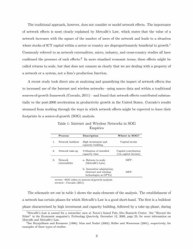
Table 1: Internet and Wireless Networks in SOGEmpirics
Process Description Where in SOG?
1. Network buildout High investment and Capital stockscapacity building
2. Network take-up Utilization of installed Capital contributioncapacity rises (via capital income)
3. Network a. Returns to scale MFPexternalities (Metcalfe’s Law)
b. Innovative adaptations(Internet and wireless MFPtechnologies as GPTs)
notes—SOG refers to sources-of-growth analysis.source—Corrado (2011)
The schematic set out in table 1 shows the main elements of the analysis. The establishment of
a network has certain phases for which Metcalfe’s Law is a good short-hand. The first is a buildout
phase characterized by high investment and capacity building, followed by a take-up phase, during
1Metcalfe’s Law is named for a researcher once at Xerox’s famed Palo Alto Research Center. See ”Beyond theEther” in the Economist magazine’s Technology Quarterly, December 12, 2009, page 23, for more information onMetcalfe and Metcalfe’s Law.
2See Brynjolfsson and Kremerer (1996); Mun and Nadiri (2002); Roller and Waverman (2001), respectively, forexamples of these types of studies.
3
which utilization of the installed capacity rises and returns to scale accrue. And because investments
in communication capital create networks inextricably linked to computing, Internet, and wireless
technologies, the capital embodies the general purpose nature of these technologies. General purpose
technologies (or GPTs) have characteristics such as high fixed costs, low reproduction costs, a ready
ability to be adapted to new uses (Bresnahan and Trajtenberg, 1995).
Communication capital then has the ability to generate high marginal returns when widely
dispersed and innovation adaptation occurs. The synergy between the GPT nature of network
technology and the scale efftects of Metcalfe’s Law suggest communication capital has significant
potential for creating network externalities.
In a sources-of-growth analysis, the direct effects of the establishment of a network is attributed
to ICT capital formation, and if the spread of high-speed networking and wireless communication
through the wider economy has created network externalities, the conventional framework will
attribute them to MFP, not ICT capital. This leads to the central question of this research: How
can network externalities be detected in a sources-of-growth analysis?
First, we can consider again the underlying forces behind the ICT boom in the 1990s. Because
internet and wireless communication technologies obtain economic value from complementary in-
vestments in ICT, much of the increase in these investments can arguably be attributed to the
expansion of networks and the possibilities they created for competitive advantage (Greenstein,
2000; Forman, Goldfarb, and Greenstein, 2003a), i.e., that the demand for Internet access was a
primary driving force behind the ICT investment boom of the late 1990s.3
Second, we can look at the productivity of capital in the provision of communications services.
Capital productivity summarizes the total impact of technology shifts and capital deepening (Hul-
ten, 1979), suggesting that the standard productivity framework can be used to develop measures
of network capital productivity and network capital utilization that can serve as detection devices
for network effects in the wider economy (Corrado, 2011). Referring back to table 1, a rise in such
indicators should be a correlate of network effects in MFP, i.e., that benefits are accruing without
the attendant costs of capital expansion.
Third, we can study econometrically whether productivity in general business picks up with
increases in Internet and wireless network use as signaled by the above-mentioned metrics.
3That it was the demand for Internet access, not the microprocessor, that was the impetus behind the late 1990sinvestment boom is argued more fully in Corrado (2011).
4

1.2 Communication Capital
Communication capital is defined as the private fixed assets used to create and power all (1) publicly
available and (2) dedicated business voice and data networks in an economy. Communication capital
thus includes all investments by service providers, including their auction purchases of wireless
spectrum, plus the private networking equipment assets used in general business.4 We now set out
the basis for our two metrics, the trend in capital productivity of networks and the utilization of
network capital for the analysis of communication capital and network effects.
Model Let industry value added in country c, industry i, and time t be denoted Yc,i,t where i = N
is the network services industry or industries. Ignoring the country and time dimension for the
moment, the network services production function can written as:
(1) YN = ANFN (LN , µKN ).
where KN is network capital at capacity, LN is labor input, and YN is the real output of network
services produced in a period. µ is capital utilization. Movements in µ reflect the underlying,
or, trend balance between network capacity and network traffic, not short-term fluctuation in de-
mand (i.e., our analysis abstracts from business cycle effects). Letting network capital productivity
YN/KN be denoted α, and using sX to denote the cost share of factor X, then the trend growth of
capital productivity ∆lnα is given by
(2) ∆lnα = ∆lnAN + ∆lnµ− sL ∗∆ln(KN/LN ).
We now show how α and µ are related to productivity in general business—the output of
all goods and services excluding the provision of network services (most easily thought of as the
nonICT-producing sector), YB =∑
i Yi,∀i 6=N . We follow the analysis of increasing returns in Basu,
Fernald, and Shapiro (2001) and assume that network services are general business inputs whose
4Computer and software assets used by business to help them connect to networks are not included because weassume they are not dedicated to creating and powering the networks but of course a case could be made for includingan unknown portion of them.
5

fixed costs CN are covered by a production function for B that exhibits increasing returns that can
be written as follows:
(3) YB = ABFB(KB, LB) = ABF′B(KB, LB)− CN
where F ′ is homogeneous of constant degree ρ(≤ 1). The return to network scale γ therefore equals
ρ(YB+CNYB
), the ratio of average costs to marginal costs, which may be greater or less than one
depending on the value for the parameter ρ and size of other quantities involved.
We further let YB relative to YN be denoted by φ(N), which is constant in steady-state growth
but is a positive function of the number of users engaged in network activity via Metcalfe’s Law
and thus increases following the establishment of a new network or introduction of new network
technology. Such increases in φ(N) can be thought of as temporarily augmenting YB relative to YN
through the productivity shift term AB.
If network fixed costs are the only source of fixed costs then CN = KN . And if fixed costs
are the only source of increasing returns—save for changes in φ(N) which by definition is constant
in steady state growth—then ρ = 1. γ is then a returns to network scale parameter that can we
written as follows:
γ =
(1 +
KN
YB
)=
(1 +
1
φ(N)α
).(4)
Recalling that the returns to scale parameter modifies factor shares as conventionally calculated
in growth accounting, changes in γ influence accelerations and decelerations in productivity, e.g.,
a fall in γ increases the rate of productivity growth (because less of the conventionally-weighted
change in factor inputs is subtracted from output change) and vice versa.
Equation (4) then implies the following: (a) sustained increases (decreases) in the capital pro-
ductivity of network services provision α are associated with increases (decreases) in productivity
change in general business; (b) changes in the factor φ—through changes in network utilization
µ—influences productivity change in a similar fashion.
If the trend in the capital productivity of network access services falls at the same time that the
size of networks grow, providers are essentially capturing network effects in their revenues (thereby
6

covering the costs of building out the network). Producer externalities associated with innovative
uses of networks would still show up in MFP and consumer externalities would still be in the
unmeasured “consumer surplus, but a falling trend in capital productivity of providers is a sign
that the net effect of network externalities may not be very large.
By the same token, a constant trend gives greater scope for these externalities, and a rising
trend even more so. In this way, equation (4) captures the “virtuous cycle” often mentioned in the
micro empirical literature on ICT spending and productivity, kicking in with full force when α and
µ are both rising.
Measurement Where do we find network capital productivity and capital utilization in the pro-
ductivity data? The relationship given by (2) is especially useful when technology is highly capital
intensive as is true in telecommunications (and the implied network services function within general
business). Even in the standard neoclassical model in which the growth in technology is exogenous,
capital deepening (the extent to which the growth of capital exceeds other inputs) is determined
endogenously, reflecting producers choice for other inputs following a change in technology. It was
in this sense that Hulten (1979) argued that capital productivity reflects the total impact of these
processes.5
In our application, capital productivity is a measure of the efficiency with which network services
are delivered and can be calculated as a Divisia index based on data for real network services output
and real network capital input. Network services includes both the publicly marketed voice and
Internet access services and the self-produced services of business local and wide area networks.
A Divisia index of capital productivity that reflects the performance of the entire network (and
both types of capital) can then be calculated using data from industry growth accounts assuming
(1) production of network services in general business uses a fixed capital share and (2) prices for
marketed network access are a good proxy for prices of network services self-produced by general
business.
As to network capital utilization, we must first be clear theoretically about how it leaves its
footprints in productivity measures. As shown by Berndt and Fuss (1986), capital productivity is
5For most industries, i.e., non-network industries, the growth of capital exceeds that of other inputs and in steady-state growth with constant returns, output moves in proportion to capital and capital productivity is constant.
7
proportional to the marginal product of capital (which varies directly with µ) and capital utilization
is absorbed in capital income and capital services as conventionally calculated (as per line 2, table
1). In other words, when productivity measures are obtained from a sources-of-growth accounting
in which the rate of return is calculated on an ex post basis (as in Jorgenson and Griliches, 1967),
capital utilization is absorbed in capital income not MFP.6
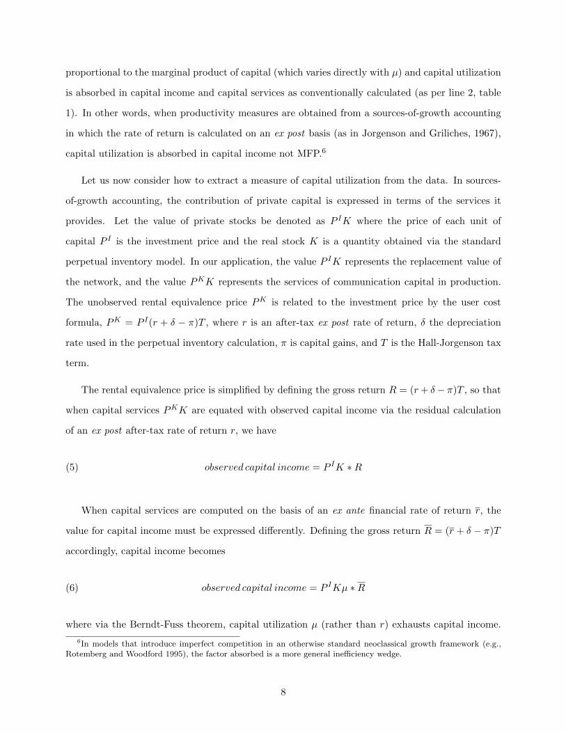
Let us now consider how to extract a measure of capital utilization from the data. In sources-
of-growth accounting, the contribution of private capital is expressed in terms of the services it
provides. Let the value of private stocks be denoted as P IK where the price of each unit of
capital P I is the investment price and the real stock K is a quantity obtained via the standard
perpetual inventory model. In our application, the value P IK represents the replacement value of
the network, and the value PKK represents the services of communication capital in production.
The unobserved rental equivalence price PK is related to the investment price by the user cost
formula, PK = P I(r + δ − π)T , where r is an after-tax ex post rate of return, δ the depreciation
rate used in the perpetual inventory calculation, π is capital gains, and T is the Hall-Jorgenson tax
term.
The rental equivalence price is simplified by defining the gross return R = (r+ δ− π)T , so that
when capital services PKK are equated with observed capital income via the residual calculation
of an ex post after-tax rate of return r, we have
(5) observed capital income = P IK ∗R
When capital services are computed on the basis of an ex ante financial rate of return r, the
value for capital income must be expressed differently. Defining the gross return R = (r + δ − π)T
accordingly, capital income becomes
(6) observed capital income = P IKµ ∗R
where via the Berndt-Fuss theorem, capital utilization µ (rather than r) exhausts capital income.
6In models that introduce imperfect competition in an otherwise standard neoclassical growth framework (e.g.,Rotemberg and Woodford 1995), the factor absorbed is a more general inefficiency wedge.
8
Equating these two expressions
P IK ∗R = P IKµ ∗R
and solving for µ yields
(7) µ =R
R≈ r
r.
which suggests the relationship between the ex post and ex ante rate of return for an industry or
sector is an indicator of its capital utilization.
Equation (7) can be used to calculate an indicator of the utilization for the publicly available
voice and data network capital (communications capital type 1). Utilization of dedicated busi-
ness networks (communications capital type 2) cannot be so readily isolated because its use is
spread across industries and its marginal productivity therefore not separable from other assets and
industry-specific factors (see Hulten, 2009, for a discussion of such issues). But as previously men-
tioned, under not too restrictive assumptions, we can calculate capital productivity for the entire
network.
2 Empirics
2.1 Data Sources
The “rolling updates” EUKLEMS industry-level productivity accounts (O’Mahony and Timmer,
2009; Timmer, O’Mahony, Inklaar, and van Ark, 2010) at www.euklems.net form the core of the
database used in this paper. The EUKLEMS rolling updates estimates use an updated industry
structure (NACE 2) in which information and communications services industries feature more
prominently. Especially relevant to this study is that now the telecommunications services indus-
try (NACE 61) is separately shown whereas previously it was combined with postal and courier
activities. NACE 61 includes providers of Internet and wireless network access.
The rolling updates productivity estimates available as of December 2013 allow us to study
market sector productivity at the industry-level (26 market sector industries) in eight EU countries:
Austria, Finland, France, Germany, Italy, Netherlands, Spain, and United Kingdom.
9
For the analysis of communications and networking technologies, it is necessary to have an
appropriate measure of real communication capital. We incorporate harmonized, quality-adjusted
investment prices for communication equipment and include purchases of 3G/LTE/ 4G wireless spec-
trum as an asset type to more accurately represent the communication capacity of EU economies;
we also incorporate the harmonized software deflator developed for the analysis of intangible invest-
ment in EU economics (Corrado, Haskel, Jona-Lasinio, and Iommi, 2013) to better represent ICT
services production. Finally, because EUKLEMS data are available only through 2009, we extend
the available growth accounts by two years, to 2011, to improve the timeliness of our analysis.
Details on these adjustments, as well as a list of included industries and a description of how
we extended the time coverage, are in an appendix. As we shall shortly see, the new EUKLEMS
accounts and quality-adjusted telecom equipment prices and spectrum data are consequential for the
analysis in this paper. Because we extend and make adjustments to underlying data, we compute
our own net stocks, capital services, and TFP estimates for each of the 26 market sector NACE
industries using the same methods as EUKLEMS. Differences between our estimates and EUKLEMS
are noted in due course.
2.2 Communication Capital Metrics
Table 2 shows rates of growth of variables related to communication capital and its utilization
contained in this dataset. Rates of growth in this table are from 1996 to 2011, with breaks at
2002/2003 and 2007/2008. The latter break begins the recent period dominated by financial crises,
fiscal austerity, and recession in Europe, whereas a break at 2002/3 is used because by then mobile
penetration reached essentially 100 percent in the countries we study and take-up of wireless 3G
networks became increasingly widespread. Before analyzing them, a comment on the detailed
telecom industry data is in order.
The distribution of communication equipment (CT) capital investment across industry sectors
varies substantially across countries in our sample. In some countries (Austria, Germany, Nether-
lands), 25 to 35 percent of private CT capital investment is by the telecom sector.7 In some others,
CT investment reportedly is not concentrated (Finland and France). In still others (Italy, Spain,
7This is also the case in the United States.
10
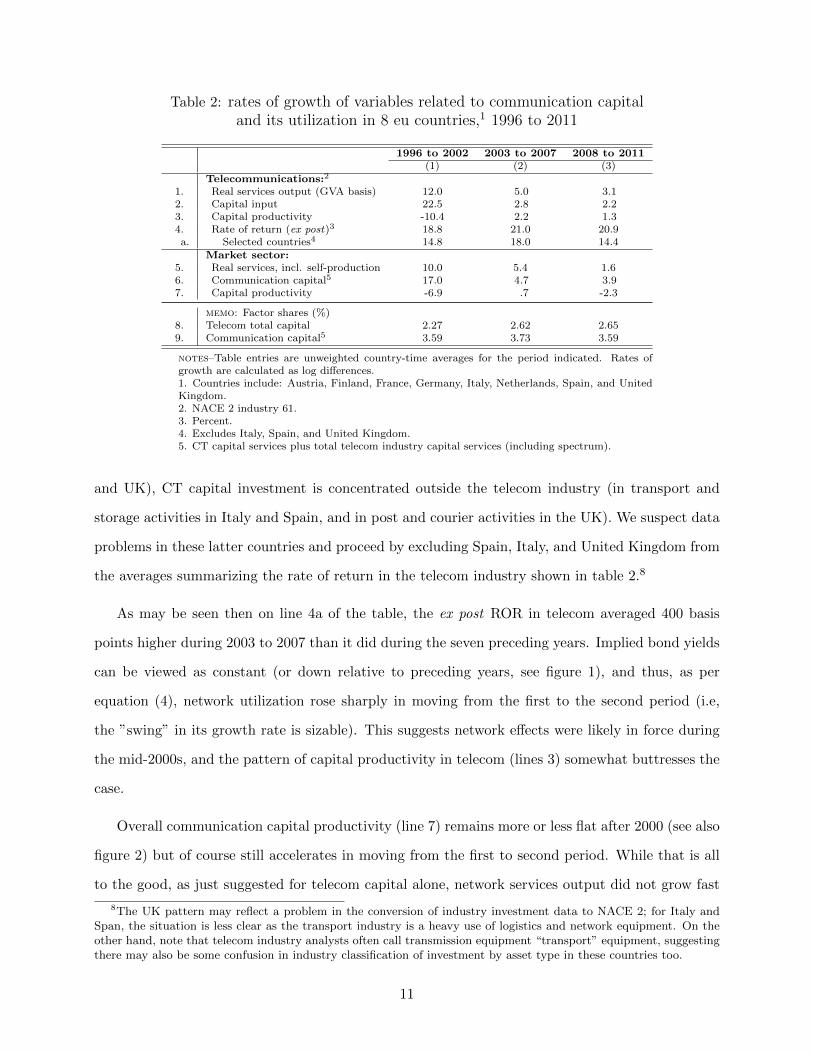
Table 2: rates of growth of variables related to communication capitaland its utilization in 8 eu countries,1 1996 to 2011
1996 to 2002 2003 to 2007 2008 to 2011(1) (2) (3)
Telecommunications:2
1. Real services output (GVA basis) 12.0 5.0 3.12. Capital input 22.5 2.8 2.23. Capital productivity -10.4 2.2 1.34. Rate of return (ex post)3 18.8 21.0 20.9a. Selected countries4 14.8 18.0 14.4
Market sector:5. Real services, incl. self-production 10.0 5.4 1.66. Communication capital5 17.0 4.7 3.97. Capital productivity -6.9 .7 -2.3
memo: Factor shares (%)8. Telecom total capital 2.27 2.62 2.659. Communication capital5 3.59 3.73 3.59
notes–Table entries are unweighted country-time averages for the period indicated. Rates ofgrowth are calculated as log differences.1. Countries include: Austria, Finland, France, Germany, Italy, Netherlands, Spain, and UnitedKingdom.2. NACE 2 industry 61.3. Percent.4. Excludes Italy, Spain, and United Kingdom.5. CT capital services plus total telecom industry capital services (including spectrum).
and UK), CT capital investment is concentrated outside the telecom industry (in transport and
storage activities in Italy and Spain, and in post and courier activities in the UK). We suspect data
problems in these latter countries and proceed by excluding Spain, Italy, and United Kingdom from
the averages summarizing the rate of return in the telecom industry shown in table 2.8
As may be seen then on line 4a of the table, the ex post ROR in telecom averaged 400 basis
points higher during 2003 to 2007 than it did during the seven preceding years. Implied bond yields
can be viewed as constant (or down relative to preceding years, see figure 1), and thus, as per
equation (4), network utilization rose sharply in moving from the first to the second period (i.e,
the ”swing” in its growth rate is sizable). This suggests network effects were likely in force during
the mid-2000s, and the pattern of capital productivity in telecom (lines 3) somewhat buttresses the
case.
Overall communication capital productivity (line 7) remains more or less flat after 2000 (see also
figure 2) but of course still accelerates in moving from the first to second period. While that is all
to the good, as just suggested for telecom capital alone, network services output did not grow fast
8The UK pattern may reflect a problem in the conversion of industry investment data to NACE 2; for Italy andSpan, the situation is less clear as the transport industry is a heavy use of logistics and network equipment. On theother hand, note that telecom industry analysts often call transmission equipment “transport” equipment, suggestingthere may also be some confusion in industry classification of investment by asset type in these countries too.
11

Figure 1: Bond yields in Europe, 1999-Q1 to 2011-Q4
enough to bring capital productivity anywhere near its pre-2000 level (as was more than the case in
the United States by 2007; see figure 3 below, reproduced from Corrado, 20119). Rather than read
too much into this finding, we continue with our empirics and discuss capital productivity again
later.
Figure 2: Communication Capital Productivity Index, eight EU countries, 1995 to 2011
9The industry concepts used for the US do not map directly to the NACE 2 categories for Europe. In the US, theTV industry is blended with telecom and Internet access providers are shown separately.
12
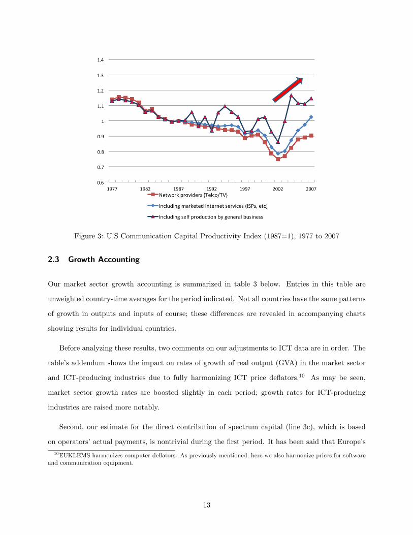
Figure 3: U.S Communication Capital Productivity Index (1987=1), 1977 to 2007
2.3 Growth Accounting
Our market sector growth accounting is summarized in table 3 below. Entries in this table are
unweighted country-time averages for the period indicated. Not all countries have the same patterns
of growth in outputs and inputs of course; these differences are revealed in accompanying charts
showing results for individual countries.
Before analyzing these results, two comments on our adjustments to ICT data are in order. The
table’s addendum shows the impact on rates of growth of real output (GVA) in the market sector
and ICT-producing industries due to fully harmonizing ICT price deflators.10 As may be seen,
market sector growth rates are boosted slightly in each period; growth rates for ICT-producing
industries are raised more notably.
Second, our estimate for the direct contribution of spectrum capital (line 3c), which is based
on operators’ actual payments, is nontrivial during the first period. It has been said that Europe’s
10EUKLEMS harmonizes computer deflators. As previously mentioned, here we also harmonize prices for softwareand communication equipment.
13
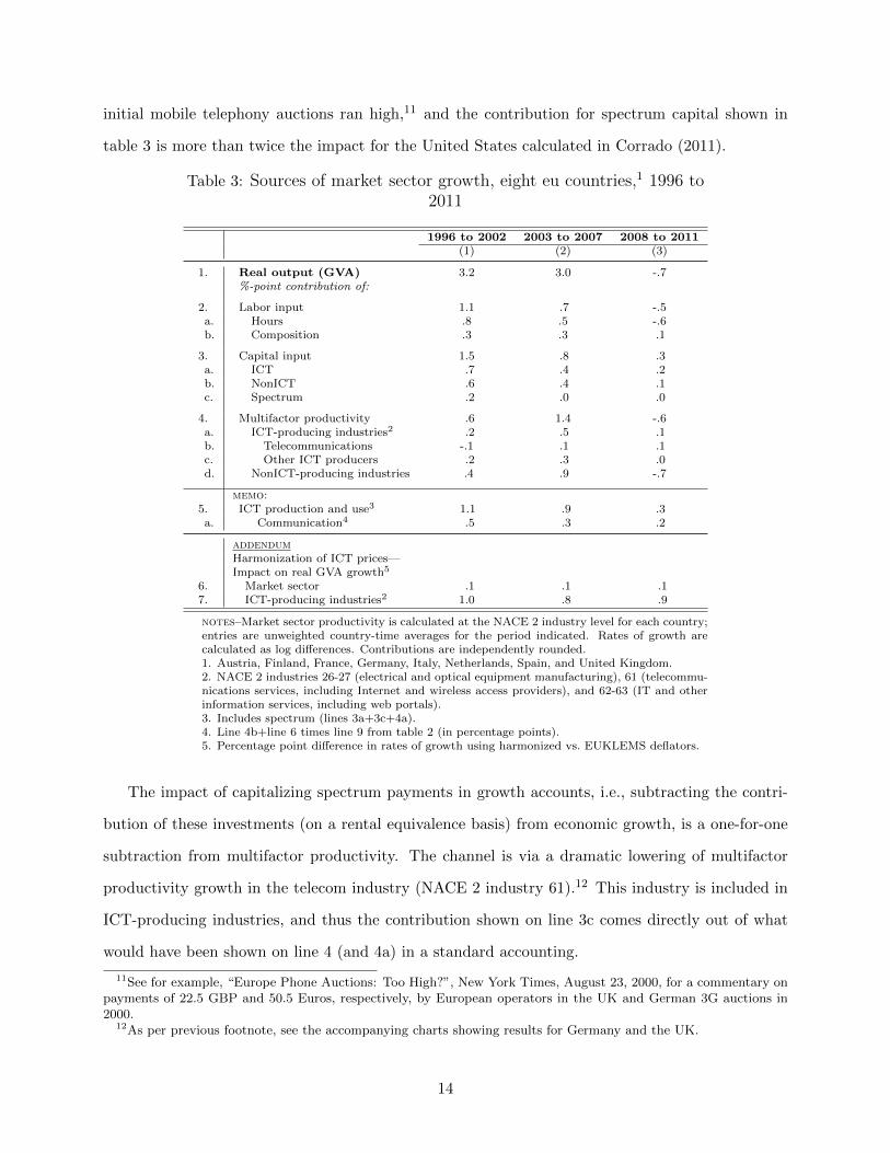
initial mobile telephony auctions ran high,11 and the contribution for spectrum capital shown in
table 3 is more than twice the impact for the United States calculated in Corrado (2011).
Table 3: Sources of market sector growth, eight eu countries,1 1996 to2011
1996 to 2002 2003 to 2007 2008 to 2011(1) (2) (3)
1. Real output (GVA) 3.2 3.0 -.7%-point contribution of:
2. Labor input 1.1 .7 -.5a. Hours .8 .5 -.6b. Composition .3 .3 .1
3. Capital input 1.5 .8 .3a. ICT .7 .4 .2b. NonICT .6 .4 .1c. Spectrum .2 .0 .0
4. Multifactor productivity .6 1.4 -.6a. ICT-producing industries2 .2 .5 .1b. Telecommunications -.1 .1 .1c. Other ICT producers .2 .3 .0d. NonICT-producing industries .4 .9 -.7
memo:5. ICT production and use3 1.1 .9 .3a. Communication4 .5 .3 .2
addendumHarmonization of ICT prices—Impact on real GVA growth5
6. Market sector .1 .1 .17. ICT-producing industries2 1.0 .8 .9
notes–Market sector productivity is calculated at the NACE 2 industry level for each country;entries are unweighted country-time averages for the period indicated. Rates of growth arecalculated as log differences. Contributions are independently rounded.1. Austria, Finland, France, Germany, Italy, Netherlands, Spain, and United Kingdom.2. NACE 2 industries 26-27 (electrical and optical equipment manufacturing), 61 (telecommu-nications services, including Internet and wireless access providers), and 62-63 (IT and otherinformation services, including web portals).3. Includes spectrum (lines 3a+3c+4a).4. Line 4b+line 6 times line 9 from table 2 (in percentage points).5. Percentage point difference in rates of growth using harmonized vs. EUKLEMS deflators.
The impact of capitalizing spectrum payments in growth accounts, i.e., subtracting the contri-
bution of these investments (on a rental equivalence basis) from economic growth, is a one-for-one
subtraction from multifactor productivity. The channel is via a dramatic lowering of multifactor
productivity growth in the telecom industry (NACE 2 industry 61).12 This industry is included in
ICT-producing industries, and thus the contribution shown on line 3c comes directly out of what
would have been shown on line 4 (and 4a) in a standard accounting.
11See for example, “Europe Phone Auctions: Too High?”, New York Times, August 23, 2000, for a commentary onpayments of 22.5 GBP and 50.5 Euros, respectively, by European operators in the UK and German 3G auctions in2000.
12As per previous footnote, see the accompanying charts showing results for Germany and the UK.
14

With this as background and as the table then shows, market sector multifactor productivity
growth picked up notably after 2002 (line 4, column 2). The pattern for ICT producers (line
4), especially telecom (line 4b), is consistent with the expected pattern when a network is being
established and then grows: productivity is held down during the first period owing to the costs of
capacity expansion and picks up later as the size of the network grows and utilization rises.
With regard to the measured contribution of ICT to economic growth and the relative role
communication in particular, comparing column (1) versus column (2), one is struck by the obser-
vation that economic growth was relatively strong at about 3 percent per year in both periods in
the 8 countries we study, and that the contribution of ICT production and use (including spectrum
capital) accounted for more than 1 percentage point per year (line 5) or nearly 40 percent of that.
The estimated direct contribution of communication (line 5a, defined as communication capital use
and telecom’s contribution to multifactor productivity change) is rather smaller; it accounts for 37
percent of the overall ICT contribution and thus for about 14 percent of economic growth (1996 to
2007).13
Note further that nonICT-producing industries contributed .5 percentage point to the post-
2002 pick up in multifactor productivity (line 4d, column 2 less column 1). Is it possible then
that European productivity growth was further boosted by salutary network effects during the mid-
2000s? The pattern we see in these results suggests this is possible. We thus turn to an econometric
analysis of whether European industries and economies enjoyed “growth dividends” or spillovers
from their investments in ICT. The foregoing suggests that we should look at communication capital
and its attendant network externalities as the underlying determinants of such effects.
3 Spillovers
We review the general case as set out in Corrado, Haskel, and Jona-Lasinio (2014), and then we
consider the special case of communication capital and network effects.
13The estimated direct contribution of communication rises to 19 percent after 2002 (i.e., calculated using theinformation shown in columns 2 and 3), with 12 percent attributed to communication capital use and 7 percentattributed to utilization effects on telecom producer productivity.
15

3.1 The General Case
Let industry value added in country c, industry i, and time t, Yc,i,t be written as:
(8) Yc,i,t = Ac,i,tFc,i(Lc,i,t,Kc,i,t).
On the right-hand side, the L’s and K’s are labour and capital services used in each industry-country
pair at time t, and A is an industry-country shift term that allows for changes in the productivity
with which inputs are transformed into output over time. L and K are represented as services
aggregates because many types of each factor are used in production. Some key distinctions among
factor types will be introduced in a moment, but for now what should be borne in mind is that both
K are L are quality-adjusted, i.e., “better” is treated as “more” via marginal product weighting.
Note then that K may be broadly defined, i.e., knowledge assets, such as R&D or other non-R&D
intangibles, could be included.
Log differentiating equation (8) gives:
(9) ∆lnYc,i,t = εLc,i,t∆lnLc,i,t + εKc,i,t∆lnKc,i,t + ∆lnAc,i,t
where εX denotes the output elasticity of an input X, which in principle varies by input, country,
industry, and time. We assume that all firms are optimizing and face identical factor inputs,
suggesting that for all firms in a given industry we may write
(10) εXc,i,t = sXc,i,t, X = L,K
where sX is the share of factor X’s payments in industry value added. So this simply writes the
first-order condition of a firm in terms of elasticities and assumes firms have no market power over
and above their ability to earn a competitive return on their capital.14
Now suppose a firm can benefit from the K in other firms or industries. Then, as Griliches
(1979, 1992) noted in the case of knowledge capital, the industry elasticity of ∆lnK on ∆lnY is a
14Note that omitting intangible capital results in what may appear to be market power or excess returns to tangiblecapital. See Corrado, Goodridge, and Haskel (2011) for further discussion.
16
mix of both internal and external elasticities. Following the generalization due to Stiroh (2002), we
write
(11) εXc,i,t = sXc,i,t + dXc,i,t, X = L,K
which says that output elasticities equal factor shares plus d, where d is any deviation of elasticities
from factor shares due to e.g., network effects (or knowledge spillovers as in the many studies of
R&D). This suggests we may write (9) as
(12) ∆lnYc,i,t = (sLc,i,t + dLc,i,t)∆lnLc,i,t + (sKc,i,t + dKc,i,t)∆lnKi,c,t + ∆lnAi,c,t.
Furthermore, following Caves, Christensen, and Diewert (1982), a Divisia TFP index can be con-
structed that is robust to an underlying translog production function so that we also have
(13) ∆lnTFPc,i,t = dLc,i,t∆lnLc,i,t + dKc,i,t∆lnKc,i,t + ∆lnAc,i,t.
Equations (12) and (13) then provide the framework for estimating spillovers to inputs to the
conventional production function (8). Note that if (8) is, say Cobb-Douglas, then ε is constant
over time and (12) might be transformed into a regression model with constant coefficients. If (8)
were, say, CES, then ε would vary over time with all input levels, and so (12) might be written as a
regression model with interactions between all the inputs. From the more structured equation (13),
a regression of ∆lnTFP on the inputs recovers direct estimates of the spillover terms. Econometric
specification and estimation issues are discussed further below.
3.2 Communication Capital and Network Effects
As previously discussed, one way to think about network effects is as increasing returns to own-
industry communication capital in which case the framework of equations (12) and (13) used by
Stiroh (2002) and Corrado et al. (2014) to look for spillovers from ICT and intangible capital is
sufficient.15 Another approach, due to Roller and Waverman (2001), is to consider the capital of
15Strictly speaking, in the case of increasing returns as previously described in Section I (see equation 4), the d-termfor network capital in equation (11) is a returns-to-scale parameter that enters multiplicatively.
17

the telecom industry akin to a country’s infrastructure, with greater telecom industry investment
associated with more efficient production in all industries. Corrado (2011) further introduced a
distinction between capacity building and an increase in network utilization, associating the latter
with the salutary effects known as “Metcalfe’s Law” discussed earlier.
The relationship between approaches that consider the special character of communication capi-
tal and the framework of equations (11), (12), and (13) can be seen by adapting the simple Griliches
(1979, 1992) model of within-industry knowledge spillover effects.
The Griliches framework relates output of the jth firm to conventional inputs, its own stock of
knowledge assets, its industry’s aggregate stock of knowledge assets, and total factor productivity.
Because the productivity of a firm depends on asset stocks of other firms, the Griliches model is
often applied by specifying transmission paths though which individual firms capture the external
benefits (e.g., geographic proximity, inter-industry input-output relationships, inter-firm employee
movements, etc.). For our application we write
(14) Qj = CT εj∑
j 6=jCT dj,c .
in which output of the jth firm Qj in country c is determined by the use of its own communication
capital CTj and the scale and utilization of communication capital of firms with whom it does
business∑
j 6=j CTj,c. The latter is expressed as all other organizations within the own country
(including telecoms, for which a distinction will be introduced shortly). Technical change, interna-
tional considerations, industry-specific inter-industry relationships, and other factors of production
are ignored for simplicity. As in the previous section, we assume that all firms are optimizing and
face identical factor prices.
If communication capital is expressed as an ex post service flow in (14), network utilization
is implicit as per Berndt and Fuss (1986) and our previous discussion. Even so, equation (14)
suggests that industry production functions relating Qi =∑
j Qj and CTi =∑
j CTj must include
additional terms to capture network externalities arising from both higher network capital utilization
and innovations stemming from increased network use. These effects can be jointly modeled as
“spillovers” from country network capacity utilization to industry productivity.
18
For any given industry then, overall network services include the private communication capital
services outside of the own industry plus the total capital services of publicly accessible network
service providers (i.e., their servers, their spectrum rights, their telephone lines, access ports, etc.).
If N denotes the network services-providing industry, then Kc,N,t is its total capital services flow.
Denote all market sector industries excluding the own industry and network service providers as
∀ i 6= (i,N). Then CTc,∀ i 6=(i,N),t is private communication capital services at time t outside of own-
industry and service-provider services.
We now are in a position to write the value added industry-level production function for each
market sector industry i 6= N as
Yc,i,t = CT ε+d1c,i,t CT
d2c,∀ i 6=(i,N),tK
d3c,N,t .(15)
From section 3.1, under cost minimization we have ε = sCTi . Compared with the conventionally
calculated impact of capital on an industry’s performance (i 6= N), equation (15) says that the
contribution of communication capital includes an own-industry effect (sCTi + d1) that is higher
than at the micro level (sCTi only) plus an extra kick (d2 + d3) stemming from the size and scope
of a country’s overall utilized communication capital.16 Collectively, the d-terms reflect network
effects.
3.3 Labor Externalities
Although this paper centers on ICT capital and why and where one might find spillovers to invest-
ments in ICT, we still need to consider externalities associated with labor input. Labor input has
a utilization dimension, emphasized in Basu and Kimball (1997) and Basu et al. (2001), which will
need to distinguish from the network effects we estimate using communication capital utilization
as a proxy. We also need to know how labor externalities (to the extent they exist) relate to the
estimates of the contribution of labor “quality” to economic growth shown in table 3.
Consider first how one might specify the labor term in spillover regression. Labor input is
usually distinguished by many types in most productivity datasets, and the contribution of labor
16Because equation (15) is expressed in value added terms, payments for telecom services have been subtracted,and thus d3 is a spillover term, not an output elasticity.
19

services is represented as the combination of a composition (“labor quality”) term Υ and hourly
labor input H and (i.e., L = Υ*H) in sources-of-growth decompositions. The composition term
reflects the net impact of the marginal-product (i.e., compensation) weighting of hours worked by
disaggregate worker type. We can further regard hours as the combination of average hours worked
Ψ and number of workers employed E (i.e., H = Ψ*E where Ψ= H/E).
Thus it seems we have three ways to represent ∆lnL when searching for spillovers. First, we
can use ∆L itself. Second, we can represent it as
∆lnLc,i,t = ∆lnΥc,i,t + ∆lnHc,i,t .(16)
Third, we might even use
∆lnLc,i,t = ∆lnΥc,i,t + ∆lnΨc,i,t + ∆lnEc,i,t .(17)
Now, when considering growth externalities, it seems natural to assume
(18) dLc,i,t∆lnLc,i,t = dLc,i,t∆lnΥc,i,t .
which says that if dLc,i,t is found to be > 0, i.e., when returns beyond the private returns paid to
labor input are detected, the underlying mechanism is externalities to upgrading the skills of the
workforce. An extra kick from “working smarter,” if you will.
We cannot, however, ignore the empirical literature on cyclical variation in productivity change.
In this literature, “working harder” also generates externalities that influence short-run productivity
change. Setting aside the term in E for the moment, if there are short-run externalities to “working
harder,” the coefficient on ∆lnΨi,c,t will not = 0 as is implicit in (18). The usual approach to
capturing this influence is to posit that changes in “effort” are positively correlated with changes
in average hours per worker. Short-run changes in the workweek of labor also arguably proxy for
changes in capital utilization, and thus overall factor utilization (Basu and Kimball, 1997; Basu,
20
Fernald, and Kimball, 2006).17 In either case we are compelled to write
(19) dLc,i,t∆lnLc,i,t = φLc,i,t∆lnΥc,i,t + ωc,i.t∆lnΨc,i.t
where φL is the coefficient of interest when searching for spillovers to human capital formation on
economic growth. We will not recover this coefficient without using ∆lnΥc,i,t as a separate regressor.
Finally, consider the ∆lnEi,c,t term. The term is obviously included when estimating a production
function; less obviously, the same holds for a TFP spillover regression to allow for increasing returns.
More generally, the foregoing implies that the ∆lnLc,i,t term needs to be specified carefully
when searching for externalities and precisely how depends on the goals and dataset of the study.
This study does not seek to identiy short-run mechansims driving productivity change. But it is
concerned with changes in network utilization. Network utilization arguably is an aspect of overall
factor utliization, which according to Basu et al. (2006) is reflected in changes in hours. For this
reason, our baseline econometric specificiation uses separate terms for changes in labor quality and
hourly labor input, i.e., we represent ∆lnLc,i,t as in (16).
3.4 Econometric Approach
Our econometric approach has two main features: First, we concentrate on estimating the direct
spillover terms, i.e., we use industry-level TFP as the dependent variable in our regressions as in
equation (13). This approach fully exploits our growth accounting dataset, which already provides
estimates of sXc,i,t for each factor input X. The approach also mitigates many of the endogeneity
issues that arise when estimating production functions (Griliches and Mairesse, 1998). Second,
we model the acceleration (or deceleration) in TFP growth rather than its first-order ln change.
This is done largely for econometric reasons, but the acceleration specification also is consistent
with the model set out in the first section of this paper, which made testable predictions regarding
productivity acceleration/deceleration based on changes in capital productivity and/or network
utilization.18
17As previously noted, ex post calculation of industry rates of return may not fully expunge the influence of factorutilization on productivity when multiple capital types with different marginal productivies are involved; again, seeHulten, 2009.
18The econometric reasons are spelled out in Corrado, Haskel, and Jona-Lasinio (2014) who work with a similardataset and find serial correlation in the residuals of TFP spillover regression equations.
21
As in our industry-based growth empirics, industry TFP is calculated using real industry GVA;
capital services K is distinguished according to two broad types, ICT capital and nonICT capi-
tal; where relevant we also account for two-way wireless spectrum. To examine the influence of
a country’s utilized communication capital on industry-level productivity as set out in equation
(15), industry-level ICT capital is further disaggregated into IT capital (computers and computer
software) and CT capital (communications/networking equipment), and we use the country-level
capital productivity series shown in figure 2 and table 2 to represent a country’s utilized communica-
tion capital. This variable is denoted Yc,N+OA,t/KCT+KNc,t where the “OA” in the notation indicates
that communication services supplied by industries on own-account are included.19
Letting ∆(∆lnTFP ) denote productivity acceleration, we experiment with two basic estimating
equations. The first is given by
∆(∆lnTFPc,i,t) = α1∆(∆lnKCTc,i,t) + α2∆(∆lnKIT
c,i,t) + α3∆(∆lnHc,i,t)(20)
+ α4∆(∆lnKNonICTc,i,t ) + α5∆(∆lnΥc,i,t) + ζi + ζc + ζt + ηi,c,t
where the ζ’s are controls for country, industry, and time effects on the change in productivity
growth, and the α’s are spillover terms. With this equation, we set out the basic relationships in
our industry growth accounts data, and we experiment with lags and report results of the impact
of disaggregating the KICT term into KIT and KCT as well as L into Υ and H. According to the
analysis leading to equation (15), we do not necessarily expect to find α1 > 0 in equation (20)
The coefficient α2 represents industry-level IT spillover effects, where matters are more nu-
anced. As previously mentioned, a micro-based literature suggests there are strong links between
IT adoption and productivity change at the firm level (Bresnahan, Brynjolfsson, and Hitt, 2002;
Brynjolfsson, Hitt, and Yang, 2002). And while the macro- and industry-level work to date is
consistent with strong links, normal returns to ICT investments typically are not rejected when
examining comprehensive industry data (e.g., Stiroh 2005; Inklaar, Timmer, and van Ark 2008).
As we have a new model suggesting alternative channels for CT—plus an updated and refined
EUKLEMS dataset (updated industry classifications, refined ICT price measures, and additional
19Note that the measurement issues discussed with regard to the industry distribution of CT capital in certaincountries do not materially affect this variable, or put differently, we do not use the difference between the ex postand ex ante RORs for the measurement reasons previously discussed.
22
years)—it seems reasonable to revisit whether industry growth accounting still captures all that is
going on with IT. We are particularly interested in whether α2 is positive and significant after 2002
(and not before), as this would be consistent with investments in IT generating a “growth dividend”
due to network effects (as well as remaining consistent with earlier findings in the literature).
The second estimating equation considers network effects as adapted for the spillover framework
via equation (15). It applies to market sector industries (i 6= N , where N is the network services-
producing industry) and is given by
∆(∆lnTFPc,i,t) = β1∆ln(Yc,N+OA,t/KCT+KNc,t ) + β2∆(∆lnKIT
c,i,t) + β3∆(∆lnHc,i,t)(21)
+ β4∆(∆lnKNonICTc,i,t ) + β5∆(∆lnΥc,i,t) + ζi + ζc + ζt + ηi,c,t
where β1 is d1 + d2 + d3 of equation (15). The value of β5 ∗∆ln(Yc,N+OA,t/KCT+KNc,t ) is then the
directly estimated contribution of network effects to productivity change. We will discuss the role
of the IT and hours term in this regression when we present our results.
4 Regression Results
All regression results use robust estimation techniques with random effects.20 We report each
regression specification for two time periods, pre- and post-2002. We split the dataset at 2002 for
the same reasons we used 2002 as a break point in the growth accounting, namely that we expect
network effects to have kicked in by then, and via Metcalfe’s Law a single linear model of ∆lnAc,i,t
is unlikely to prevail pre- and post- widespread use of wireless and Internet-based networks for the
conduct of business. We did not determine that the sample is best split at 2002 rather than 2001
or 2003, though we do find that no break in structure is rejected according to simple F–tests for
the regression pairs (vs regressions for the combined sample) shown in the tables that follow.21
20We have detected outliers and clusters of outliers based on the evaluation of the predicted fit, the Cooks distance,simple scatter plots, and tables comparing the mean with the maximum value and the minimum value. The presenceof outliers in the dataset can strongly distort the estimators and lead to unreliable results. Robust regression issensitive to outliers and the best model to use when errors are not identically distributed.
21Results for the combined sample and for the F–tests are available from the authors upon request.
23
4.1 Preliminaries
We first review our baseline regression specification, discussing how we treat the labor term and
then, because spillovers may take time, the results of our experimentation with lags. Table 5 reports
results of these preliminary investigations. When equation (20) is estimated with a contemporane-
ous labor services term, the estimated coefficients are negative and significant (columns 1 and 2).
When the labor services term is lagged, however, the estimated externality coefficients turn positive
(columns 3 and 4). Moreover, they are significant in both periods.
When the labor services term is then disaggregated (columns 5 and 6), the underlying mechanism
for the term’s significant externality coefficient is seen to be rather different in the two periods—
namely, only the hours effect is significant in the first period whereas “working smarter” rules in the
second. This finding may may reflect improvements in labor input data beginning in 2002 rather
than signaling these effects are truly only present after then.22
The estimated spillover to increases in labor quality is robust to specification change, however,
as will become clear as results of changing other aspects of our regressions are presented. For
example, the capital terms are also lagged in columns 7 and 8, a specification that allows spillovers
to “take time” for all factors, not just labor. And as may be seen—focussing on the labor terms
for the moment—very little changes (this also is true when the labor terms are lagged two periods,
not shown). All told, these results imply that, above and beyond the estimated direct contribution
of improvements in workforce skills to productivity since 2002 (about 0.2 percentage points per
year), there has been an additional small boost—0.06 percentage points per year, on average—due
to externalities.
How does this pertain to our story for ICT? Not much in that we get essentially the same
regression coefficients for the capital terms no matter the specification for the labor term(s).23 But
of particular note, when we shift to the specification with consistent lags on all terms, the statistical
significance of the ICT spillover term becomes stronger the second period (although it’s size is just
22The labor force survey (LFS) data used to determine labor composition in the “rolling updates” version ofEUKLEMS are generally available from 2002 onwards, whereas estimates for previous years are based on other (albeitrelated) sources. EUKLEMS documentation also states that it was necessary to concord industry labor compositionindexes from NACE 1 to NACE 2 prior to 2002, so data conversion may also be playing a role.
23True, when the capital terms are lagged the small negative coefficient on nonICT capital turns significant, whichis difficult to rationalize, except to note that the estimated impact is very, very small relative to nonICT capital’sfactor share (about 20 percent in our sample).
24
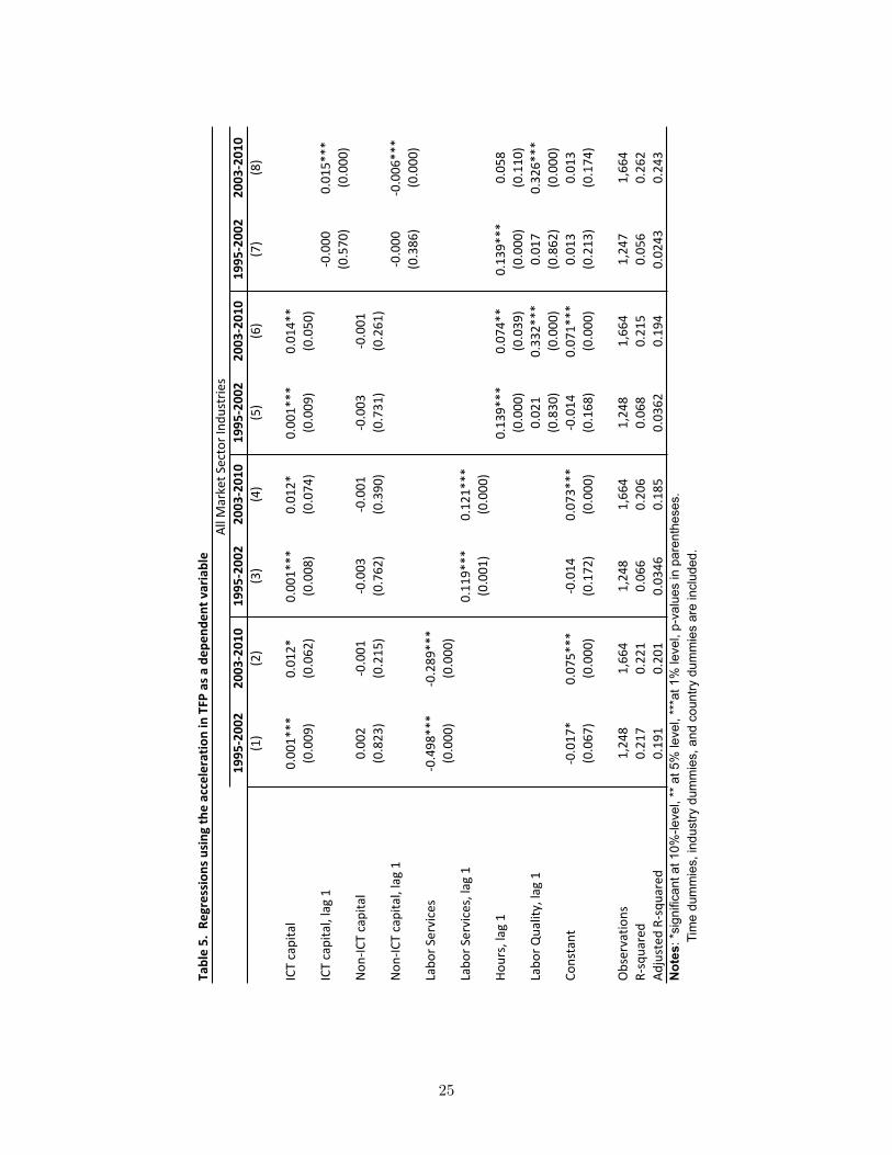
Table 5. R
egressions using th
e acceleratio
n in TFP as a
dep
ende
nt variable
1995-‐2002
2003-‐2010
1995-‐2002
2003-‐2010
1995-‐2002
2003-‐2010
1995-‐2002
2003-‐2010
(1)
(2)
(3)
(4)
(5)
(6)
(7)
(8)
ICT capital
0.001***
0.012*
0.001***
0.012*
0.001***
0.014**
(0.009
)(0.062
)(0.008
)(0.074
)(0.009
)(0.050
)ICT capital, lag 1
-‐0.000
0.015***
(0.570
)(0.000
)Non
-‐ICT capital
0.002
-‐0.001
-‐0.003
-‐0.001
-‐0.003
-‐0.001
(0.823
)(0.215
)(0.762
)(0.390
)(0.731
)(0.261
)Non
-‐ICT capital, lag 1
-‐0.000
-‐0.006***
(0.386
)(0.000
)Labo
r Services
-‐0.498***
-‐0.289***
(0.000
)(0.000
)Labo
r Services, lag 1
0.119***
0.121***
(0.001
)(0.000
)Ho
urs, lag 1
0.139***
0.074**
0.139***
0.058
(0.000
)(0.039
)(0.000
)(0.110
)Labo
r Quality, lag 1
0.021
0.332***
0.017
0.326***
(0.830
)(0.000
)(0.862
)(0.000
)Co
nstant
-‐0.017
*0.075***
-‐0.014
0.073***
-‐0.014
0.071***
0.013
0.013
(0.067
)(0.000
)(0.172
)(0.000
)(0.168
)(0.000
)(0.213
)(0.174
)
Observatio
ns1,248
1,664
1,248
1,664
1,248
1,664
1,247
1,664
R-‐squared
0.217
0.221
0.066
0.206
0.068
0.215
0.056
0.262
Adjusted
R-‐squ
ared
0.191
0.201
0.0346
0.185
0.0362
0.194
0.0243
0.243
T
ime
dum
mie
s, in
dust
ry d
umm
ies,
and
cou
ntry
dum
mie
s ar
e in
clud
ed.
Notes
: *si
gnifi
cant
at 1
0%-le
vel,
** a
t 5%
leve
l, **
*at 1
% le
vel,
p-va
lues
in p
aren
thes
es.
All M
arket S
ector Ind
ustries
25
about the same). What does this imply? A great deal, as it suggests that industry-level productivity
spillovers to ICT investment registered as large as 0.11 percentage point per year after 2002 (.15 ∗
7.2 percent average annual growth rate of ICT capital).
We now argue that network externalities are the underlying mechanism for this effect and that
the total impact of network effects between 2003 and 2007 was larger still.
4.2 IT Spillovers and Network Effects
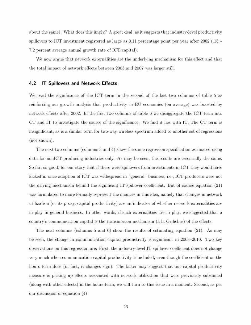
We read the significance of the ICT term in the second of the last two columns of table 5 as
reinforcing our growth analysis that productivity in EU economies (on average) was boosted by
network effects after 2002. In the first two columns of table 6 we disaggregate the ICT term into
CT and IT to investigate the source of the significance. We find it lies with IT. The CT term is
insignificant, as is a similar term for two-way wireless spectrum added to another set of regressions
(not shown).
The next two columns (columns 3 and 4) show the same regression specification estimated using
data for nonICT-producing industries only. As may be seen, the results are essentially the same.
So far, so good, for our story that if there were spillovers from investments in ICT they would have
kicked in once adoption of ICT was widespread in “general” business, i.e., ICT producers were not
the driving mechanism behind the significant IT spillover coefficient. But of course equation (21)
was formulated to more formally represent the nuances in this idea, namely that changes in network
utilization (or its proxy, capital productivity) are an indicator of whether network externalities are
in play in general business. In other words, if such externalities are in play, we suggested that a
country’s communication capital is the transmission mechanism (a la Griliches) of the effects.
The next columns (columns 5 and 6) show the results of estimating equation (21). As may
be seen, the change in communication capital productivity is significant in 2003–2010. Two key
observations on this regression are: First, the industry-level IT spillover coefficient does not change
very much when communication capital productivity is included, even though the coefficient on the
hours term does (in fact, it changes sign). The latter may suggest that our capital productivity
measure is picking up effects associated with network utilization that were previously subsumed
(along with other effects) in the hours term; we will turn to this issue in a moment. Second, as per
our discussion of equation (4)
26
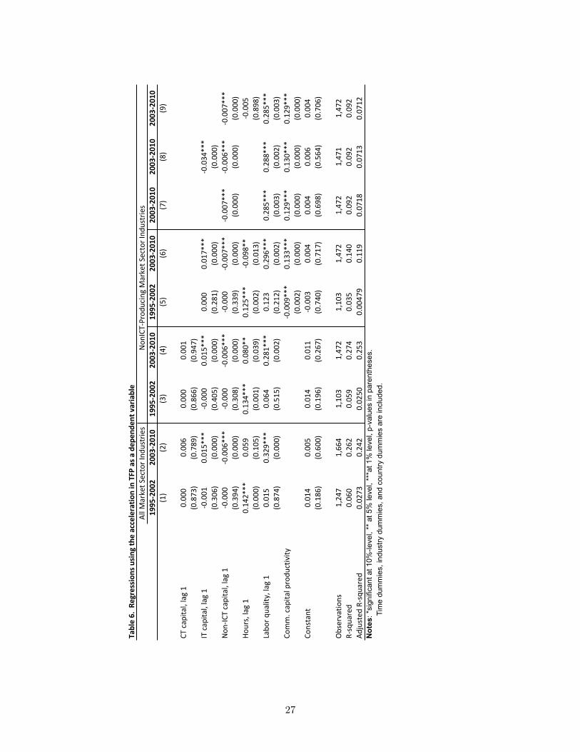
Table 6. R
egressions using th
e acceleratio
n in TFP as a
dep
ende
nt variable
1995-‐2002
2003-‐2010
1995-‐2002
2003-‐2010
1995-‐2002
2003-‐2010
2003-‐2010
2003-‐2010
2003-‐2010
(1)
(2)
(3)
(4)
(5)
(6)
(7)
(8)
(9)
CT capita
l, lag 1
0.000
0.006
0.000
0.001
(0.873
)(0.789
)(0.866
)(0.947
)IT capita
l, lag 1
-‐0.001
0.015***
-‐0.000
0.015***
0.000
0.017***
-‐0.034***
(0.306
)(0.000
)(0.405
)(0.000
)(0.281
)(0.000
)(0.000
)Non
-‐ICT capital, lag 1
-‐0.000
-‐0.006***
-‐0.000
-‐0.006***
-‐0.000
-‐0.007***
-‐0.007***
-‐0.006***
-‐0.007***
(0.394
)(0.000
)(0.308
)(0.000
)(0.339
)(0.000
)(0.000
)(0.000
)(0.000
)Ho
urs, lag 1
0.142***
0.059
0.134***
0.080**
0.125***
-‐0.098**
-‐0.005
(0.000
)(0.105
)(0.001
)(0.039
)(0.002
)(0.013
)(0.898
)Labo
r quality, lag 1
0.015
0.329***
0.064
0.281***
0.123
0.296***
0.285***
0.288***
0.285***
(0.874
)(0.000
)(0.515
)(0.002
)(0.212
)(0.002
)(0.003
)(0.002
)(0.003
)Co
mm. capita
l produ
ctivity
-‐0.009***
0.133***
0.129***
0.130***
0.129***
(0.002
)(0.000
)(0.000
)(0.000
)(0.000
)Co
nstant
0.014
0.005
0.014
0.011
-‐0.003
0.004
0.004
0.006
0.004
(0.186
)(0.600
)(0.196
)(0.267
)(0.740
)(0.717
)(0.698
)(0.564
)(0.706
)
Observatio
ns1,247
1,664
1,103
1,472
1,103
1,472
1,472
1,471
1,472
R-‐squared
0.060
0.262
0.059
0.274
0.035
0.140
0.092
0.092
0.092
Adjusted
R-‐squ
ared
0.0273
0.242
0.0250
0.253
0.00479
0.119
0.0718
0.0713
0.0712
Notes
: *si
gnifi
cant
at 1
0%-le
vel,
** a
t 5%
leve
l, **
*at 1
% le
vel,
p-va
lues
in p
aren
thes
es.
T
ime
dum
mie
s, in
dust
ry d
umm
ies,
and
cou
ntry
dum
mie
s ar
e in
clud
ed.
All M
arket S
ector Ind
ustries
Non
ICT-‐Prod
ucing Market S
ector Ind
ustries
27
in section 1, the coefficient on communication capital productivity has the expected sign in the
second period, which supports the model and analysis of network effects set forth in this paper.24
To rule out the possibility that the coefficient on capital productivity is imprecisely estimated
due to collinearity with hours (or IT), the next three columns (7–9) show alternative regressions for
the second period in which the hours and/or IT term is dropped. As may be seen the coefficient
on capital productivity remains stable, whereas the coefficient on IT appears to be sensitive to
whether hours is included. This does not necessarily signal that the coefficient on IT is imprecisely
estimated, but rather that accounting for changes in hours—especially when controlling for country-
level network utilization—seems to be important for picking up spillovers to IT at the industry-level.
Column 6’s estimate of network effects—the regression coefficient on communication capital
productivity—stems only from the country-time variation in our dataset. We previously argued
that our finding of IT spillovers after 2002 (and only after 2002) may also be capturing network
effects to the extent such effects are differentiated at the industry level by IT capital. Recall, too,
that IT capital includes computer software, which may be serving as a proxy for complementary
investments in other forms of intangible capital. In a recent study using industry-level productivity
data from EUKLEMS and intangible investment data from INTAN-Invest, ICT and intangible cap-
ital (excluding software) have been shown to be complements in production (Corrado, Haskel, and
Jona-Lasinio, 2014). The possibility that industries with relatively fast-growing stocks of software
capital are getting more out of their overall ICT investments because of complementary investments
in intangible capital is then very plausible. The intangible capital story does not explain, however,
why this happens after 2002 and not before (when intangible investments were growing, like ICT,
much faster).
All told then, taken literally, the results in column 6 of table 6 suggest that total factor productiv-
ity growth was boosted by 0.09 percentage points per year from 2003 to 2007 due to network effects
associated with utilization change (.133 ∗ 0.7 percent per year growth in communication capital
productivity) and as much as 0.13 percentage points per year from network-induced externalities to
24The coefficient on capital productivity is negative (and significant) in the first period and likely suggests thatthe period’s sharp drop in capital productivity, due in large part to massive investments in wireless spectrum intwo countries (Germany and the UK), did not negatively impact nonICT producing industries. In other words, thenegative drag on productivity in the telecom industry due to investments in wireless spectrum was offset elsewhere inbusiness.
28
IT investments (.017 ∗ 8.2 percent growth in IT capital from 2002 to 2006). Relative to the change
in total factor productivity, the total impact of these effects is substantial, accounting for nearly 25
percent of the change in total factor productivity (and more than 40 percent of its acceleration).
Because a drop in network utilization exerts a drag after 2007, over the period extended to include
the global financial crisis (i.e., 2003 to 2011), the estimated contribution of network externalities to
the change in total factor productivity, on net, washes out.25 These contributions to productivity
growth estimated for the EU are, in terms of fractions, generally comparable to those estimated for
the United States by Corrado (2011).
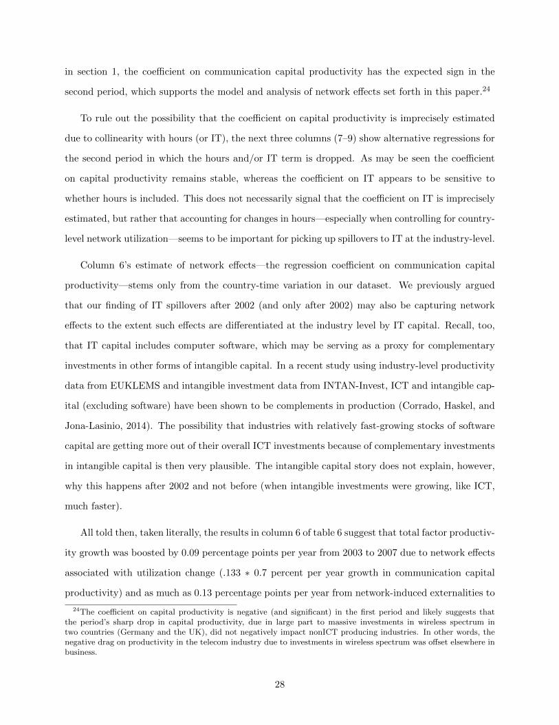
Figure 4 shows the estimated network effects in relation to the other ICT-related contributions
introduced with the growth accounting. As may be seen, the effects are rather large and significantly
enhance the estimated contribution of ICT to EU growth during the mid-2000s. The estimate of a
drag from network effects during the financial crisis is a direct outcome of a drop in the production
of network services, which includes purchased services as well as self-production (or production on
own account in the language of national accounts).
Figure 4: ICT-Related Contributions to Economic Growth in eight EU Countries.
How robust are our estimates of the size and significance of network effects? The estimates are
the product of a Griliches-inspired approach to estimating productivity spillovers to ICT investment,
25Recall from table 2 that communication capital productivity fell after 2007. The influence of IT capital spilloversis still positive, but it wanes with a post-2007 slowdown in IT capital growth (4.4 percent per year).
29
and we believe we showed them stable to specification changes and scope of variables used. The
econometric approach followed Griliches and Mairesse (1998) in using TFP as a dependent variable
(to avoid certain endogeniety problems) and also that of Corrado, Haskel, and Jona-Lasinio (2014)
in modeling its acceleration (to avoid biases due to serial correlation in the dataset used). After
finding that the lags of industry-level inputs worked better or just as well as contemporaneous terms,
we settled on a simple specification using one lag of industry-level inputs for estimating spillovers
and testing the implications of our model. The explanatory variables in our regressions are not
endogenous, and their double-differenced specification is typically thought to magnify sensitivity to
measurement error, yet we obtain strong results.26
We obtained, we believe, new findings on spillovers and network effects using EUKLEMS data for
two reasons: one, we followed the strict logic and insights of the section I.B model of communication
capital and, two, we used an improved dataset. Recall we incorporated refined ICT price measures
into EUKLEMS, and the “rolling updates” version includes data innovations especially relevant to
this study: updated measures of labor quality (after 2002) and industry classifications better suited
for the analysis of ICT.
What do these estimates suggest about possibilities for ICT-driven growth in Europe in the
future? The last fifteen years have seen the emergence of new Internet and wireless platforms in
some but not all industries (e.g., e-commerce and social networking but not homebuilding or metal-
working). The distinctive characteristic of Internet platforms as a business model is scalability—the
capability of serving additional users at very low costs, i.e., the capability for generating network
externalities. We don’t see the outward signs of very large increases in Internet use for competi-
tive advantage in our communication capital metrics for the 8 EU countries we study, i.e., capital
productivity does not materially rise as would be expected with successful Internet engagement,
widespread use of scalable platforms as a business model, and exploitation of consumer smartphone
use. But where capital productivity did rise sharply (e.g., Finland), industry productivity benefited
consequentially.
The findings in this study of 8 EU countries accords rather well with the related U.S. study by
Corrado (2011) in which it was found that capital productivity rose sharply and that productivity
26The capital productivity term includes total market sector CT capital, which of course covers each industry, andthus a very small portion of communication capital is own-industry and arguably endogenous. The logic of the model,however, is that own-industry CT capital has little bearing on the value of entire network, much less a correlate ordeterminant of network size. Thus it seems valid to treat this term as exogenous.
30
accelerated in industries relatively advanced in their degree of Internet engagement. The identify-
ing information for Internet engagement was the relative size of the installed base business process
productivity-enhancing software in 2000 (in contrast with, say, software for email and word process-
ing; see Forman, Goldfarb, and Greenstein, 2003b for further details). Our econometric analysis of
spillovers used disaggregate information on ICT and found a statistically significant ”extra” contri-
bution to EU industry productivity from investments in IT after 2002 that we interpret in a similar
manner. In other words, the estimated impacts are attributed to network effects and are material
to the estimated overall size of these effects.
5 Conclusion
This paper studied the channels through which communication networks—their capital and the
externalities they generate—affect productivity growth. Using a 17 year sample of 26 market sector
industries in 8 EU countries, we generated metrics, growth accounts, and regression results that
document the importance of communication networks and network externalities. The effects were
found to be rather important, and along with the usual channels included in ICT analysis, underscore
the importance of ICT in driving economic growth (or the lack of it) in Europe since 2002 (see again
figure 4).
All told, many subtleties are involved in how investments in networks impact productivity, and
we believe one of our major contributions has been to underscore the fact that, if the Internet
and wireless networks are the highways of the modern age (on which traffic is growing at explosive
rates worldwide), we need to use models and data that are up to the task of analyzing their
macroeconomic impacts. Related work (Corrado et al., 2014) addresses spillovers to intangibles and
how these investments that are complementary to ICT fit into the macro-productivity picture. But
as far as we know no one has looked at the issues we address in this work on communication.
References
Basu, S., J. G. Fernald, and M. S. Kimball (2006). Are technology improvements contractionary?
American Economic Review 96 (5), 1418–1448.
31

Basu, S., J. G. Fernald, and M. D. Shapiro (2001). Productivity growth in the 1990s: technology,
utilization, or adjustment? In Carnegie-Rochester conference series on public policy, Volume 55,
pp. 117–165. Elsevier.
Basu, S. and M. S. Kimball (1997). Cyclical productivity with unobserved input variation. Working
Paper 5915, National Bureau of Economic Research.
Berndt, E. R. and M. A. Fuss (1986). Productivity measurement with adjustments for variations in
capacity utilization and other forms of temporary equilibrium. Journal of Econometrics 33 (1),
7–29.
Bresnahan, T. F., E. Brynjolfsson, and L. M. Hitt (2002). Information technology, workplace
organization, and the demand for skilled labor: Firm-level evidence. Quarterly Journal of Eco-
nomics 117 (1), 339–376.
Bresnahan, T. F. and M. Trajtenberg (1995). General purpose technologies ‘Engines of growth?’.
Journal of Econometrics 65 (1), 83–108.
Brynjolfsson, E., L. M. Hitt, and S. Yang (2002). Intangible assets: Computers and organizational
capital. Brookings Papers on Economic Activity 2002:1, 137–198.
Brynjolfsson, E. and C. F. Kremerer (1996). Network externalities in microcomputer software: An
econometric analysis of the spreadsheet market. Management Science 42 (12), 1627–1647.
Byrne, D. and C. Corrado (2007). Quality-adjusted prices for communication equipment: History
and recent developments. Paper presented at the CRIW workshop at the 2007 NBER Summer
Institute.
Caves, D. W., L. R. Christensen, and W. E. Diewert (1982). The economic theory of index numbers
and the measurement of input, output, and productivity. Econometrica 50 (6), 1393–1414.
Corrado, C. (2011). Communication capital, Metcalfe’s law, and U.S. productivity growth. Eco-
nomics Program Working Paper 11-01, The Conference Board, Inc., New York.
Corrado, C., P. Goodridge, and J. Haskel (2011). Constructing a price deflator for R&D: Calculating
32

the price of knowledge investments as a residual. Working paper, Economics Program Working
Paper 11-03, The Conference Board, Inc. New York.
Corrado, C., J. Haskel, and C. Jona-Lasinio (2014). Knowledge spillovers, ICT, and productivity
growth. Working paper, The Conference Board, Imperial College, LUISS and ISTAT.
Corrado, C., J. Haskel, C. Jona-Lasinio, and M. Iommi (2012). Intangible capital and growth in ad-
vanced economies: Measurement and comparative results. Working paper available at www.intan-
invest.net.
Corrado, C., J. Haskel, C. Jona-Lasinio, and M. Iommi (2013). Innovation and intangible investment
in Europe, Japan, and the United States. Oxford Review of Economic Policy 29 (2), 261–286.
Forman, C., A. Goldfarb, and S. Greenstein (2003a). The geographic dispersion of commercial in-
ternet use. In S. Wildman and L. Cranor (Eds.), Rethinking Rights and Regulations: Institutional
Responses to New Communication Technologies, pp. 113–45. MIT Press.
Forman, C., A. Goldfarb, and S. Greenstein (2003b). Which industries use the internet? In M. Baye
(Ed.), Organizing the New Industrial Economy, Advances in Applied Microeconomics, Vol. 12,
pp. 47–72. Elsevier.
Greenstein, S. (2000). Building and delivering the virtual world: Commercializing services for
internet access. Journal of Industrial Economics 48 (4), 391–411.
Griliches, Z. (1979). Issues in assessing the contribution of research and development to productivity
growth. Bell Journal of Economics 10 (1), 92–119.
Griliches, Z. (1992). The search for R&D spillovers. Scandinavian Journal of Eco-
nomics 94 (Supplement), S29–47.
Griliches, Z. and J. Mairesse (1998). Production functions: The search for identification. In
S. Steinar (Ed.), Econometrics and Economic Theory in the twentieth century: The Ragnar
Frisch Centennial Symposium. Cambridge University Press.
Hulten, C. (1979). On the ’importance’ of productivity change. American Economic Review 69 (1),
126–36.
33

Hulten, C. (2009). Growth accounting. Working paper, NBER Working Paper 15341 (September).
Inklaar, R., M. P. Timmer, and B. van Ark (2008). Market services productivity across Europe and
the US. Economic Policy 23 (53), 139–194.
Jorgenson, D. W. and Z. Griliches (1967). The explanation of productivity change. The Review of
Economic Studies 34 (3), 249–283.
Mun, S. B. and M. I. Nadiri (2002). Information technology externalities: Empirical evidence from
42 us industries. Working paper, NBER Working Paper 9272 (October).
O’Mahony, M. and M. P. Timmer (2009). Output, input and productivity measures at the industry
level: the EU KLEMS database. Economic Journal 119 (538), F374–F403.
Roller, L. H. and L. Waverman (2001). Telecommunications infrastructure and economic develop-
ment: A simultaneous approach. American Economic Review 91 (4), 909–923.
Stiroh, K. J. (2002). Are ICT spillovers driving the new economy? Review of Income and
Wealth 48 (1), 33–57.
Stiroh, K. J. (2005). Reassessing the impact of IT in the production function: A meta-analysis and
sensitivity tests. Annals of Economics and Statistics (79/80), 529–561.
Timmer, M. P., M. O’Mahony, R. Inklaar, and B. van Ark (2010). Economic Growth in Europe.
Cambridge University Press.
34

APPENDIX
A.1 Extension of EUKLEMS to 2011
Our main data source is the EU KLEMS database (rolling updates, accessed December 2013).
EU KLEMS provides output, input, productivity, investment and capital stocks based on the new
international ISIC Revision 4 industry classification, which is consistent with the European NACE
2 industry classification (34 industries) up to the year 2009 for the following countries: Austria,
Finland, France, Germany, Netherlands, Spain, Italy, and the United Kingdom. In this study we
work with the 26 market sector industries listed in table A1. Note that “rolling updates” EUKLEMS
does not report growth accounting results for market vs. non-market sector aggregates, and thus
the aggregate market sector results reported herein are new with the database constructed for this
study.
To compute growth accounts through 2011, most value added, labor compensation, hours
worked, and gross fixed capital formation (GFCF) series at the industry level were updated with
corresponding data from the OECD’s STAN database, Eurostat, or from Haver Analytics. When
industry level GFCF data were not available from the above sources, series were approximated based
on the overall GFCF for the country, shared out by industry according to shares in the preceding
three years. Capital stocks were then extended to 2011 using the perpetual inventory method using
the same service lives used in EUKLEMS. Our capital stocks for IT, CT, and computer software
differ from EU KLEMS because we use our own harmonized price deflators for these asset types
(see section A.2). Industry level labor composition effects were extrapolated based on the average
growth rate of the preceding three years.
A.2 Addition of spectrum capital
We treated purchased wireless communication spectrum as an individual asset type in our produc-
tivity analysis, i.e., spectrum is included along with seven usual asset types: the three ICT types
(computers, computer software, and communications equipment) plus machinery, transportation
equipment, structures, and other assets. Note that residential structures is an eighth asset type in
EUKLEMS, but it is excluded along with the real estate industry from the analysis conducted in
this paper.
35

Table A1: Market Sector Industry List
Industry Code
1 Agriculture, Forestry and Fishing A2 Mining and Quarrying B3 Food products, beverages and tobacco 10-124 Textiles, wearing apparel, leather and related prodcuts 13-155 Wood and paper products; printing and reproduction of recorded media 16-186 Coke and refined petroleum products 197 Chemicals and chemical products 20-218 Rubber and plastics products, and other non-metallic mineral products 22-239 Basic metals and fabricated metal products, except machinery and equipment 24-2510 Electrical and optical equipment 26-2711 Machinery and equipment n.e.c. 2812 Transport equipment 29-3013 Other manufacturing; repair and installation of machinery and equipment 31-3314 Electricity, Gas and Water Supply D-E15 Construction F16 Wholesale and retail trade and repair of motor vehicles and motorcycles 4517 Wholesale trade, except of motor vehicles and motorcycles 4618 Retail trade, except of motor vehicles and motorcycles 4719 Transport and storage 49-5220 Postal and courier activities 5321 Accomodation and Food Service Activities I22 Publishing, audiovisual and broadcasting activities 58-6023 Telecommunications 6124 IT and other information services 62-6325 Financial and Insurance Activities K26 Professional Scientific, Technical, Administrative and Support Service Activities M-N
note–For the full list of NACE 2 industries, see http://epp.eurostat.ec.europa.eu/cache/ITY_
OFFPUB/KS-RA-07-015/EN/KS-RA-07-015-EN.PDF
Spectrum purchases figures for our eight countries are from various sources, including the ITU,
Ofcom, and PWC. Prices paid in 3G/LTE/4G wireless spectrum auctions are regarded as nominal
investment. Nominal investment was translated into real investment using gross output deflators for
the telecommunications industry obtained from OECD STAN. These deflators were not available
for Germany, Spain, and UK, and we used the value added prices in EUKLEMS. Finally, capital
stocks were calculated using the perpetual inventory method assuming a zero rate of depreciation
(i.e., constant productivity as it “ages” and no discards or retirements).
Among market sector industries, broadband spectrum is owned in the telecommunications ser-
vices industry only. (Note that we do not measure traditional wireless radio and television spec-
trum.) Table A2 sets out the resulting values for ICT and wireless spectrum factor shares in our
industry-level dataset (i.e., these are country-time averages of industry-level value added shares).
As may be seen the values for spectrum capital are small relative to ICT in the aggregate market
economy but loom rather large in the telecom industry.
36
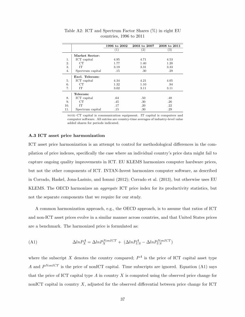
Table A2: ICT and Spectrum Factor Shares (%) in eight EUcountries, 1996 to 2011
1996 to 2002 2003 to 2007 2008 to 2011(1) (2) (3)
Market Sector:1. ICT capital 4.95 4.71 4.532. CT 1.77 1.40 1.203. IT 3.19 3.31 3.334. Spectrum capital .15 .30 .29
Excl. Telecom:5. ICT capital 4.34 4.21 4.056. CT 1.32 1.10 .947. IT 3.02 3.11 3.11
Telecom:8. ICT capital .64 .50 .489. CT .45 .30 .26
10. IT .17 .20 .2211. Spectrum capital .15 .30 .29
note–CT capital is communication equipment. IT capital is computers andcomputer software. All entries are country-time averages of industry-level valueadded shares for periods indicated.
A.3 ICT asset price harmonization
ICT asset price harmonization is an attempt to control for methodological differences in the com-
pilation of price indexes, specifically the case where an individual country’s price data might fail to
capture ongoing quality improvements in ICT. EU KLEMS harmonizes computer hardware prices,
but not the other components of ICT. INTAN-Invest harmonizes computer software, as described
in Corrado, Haskel, Jona-Lasinio, and Iommi (2012); Corrado et al. (2013), but otherwise uses EU
KLEMS. The OECD harmonizes an aggregate ICT price index for its productivity statistics, but
not the separate components that we require for our study.
A common harmonization approach, e.g., the OECD approach, is to assume that ratios of ICT
and non-ICT asset prices evolve in a similar manner across countries, and that United States prices
are a benchmark. The harmonized price is formulated as:
(A1) ∆lnPAX = ∆lnPNonICTX + (∆lnPAUS −∆lnPNonICTUS )
where the subscript X denotes the country compared; PA is the price of ICT capital asset type
A and PNonICT is the price of nonICT capital. Time subscripts are ignored. Equation (A1) says
that the price of ICT capital type A in country X is computed using the observed price change for
nonICT capital in country X, adjusted for the observed differential between price change for ICT
37

capital type A and price change for nonICT capital in the United States.
We proceed as follows: (1) we use the ITAN-Invest software deflator (available at www.INTAN-
Invest.org); (2) we apply equation (A1) and obtain quality-adjusted deflators for both telecom
equipment and computers. For computers we use the U.S. BEA’s quality-adjusted computer price
deflator and for telecom equipment we use the investment price originally developed in Byrne and
Corrado (2007) and which is regularly updated by the Federal Reserve.27 As to congruent output
prices, we make small adjustments to components of the ICT manufacturing value added deflators
(components of NACE 26). We do not have an industry software output price from INTAN-Invest.28
Our results for computer prices are virtually identical to EUKLEMS whereas the results for telecom
equipment exhibit rates of price change that decline, rather than rise. The country-time average of
the annual price change differential from 1996 to 2011 is more than 5 percentage points.
27The 2011 annual revision of the U.S. national accounts incorporated many of the Byrne-Corrado communicationequipment price indexes from 2002 on.
28INTAN-Invest harmonizes software output prices at the market sector level defined according to NACE 1 indus-tries, and it is unclear how to apply its adjustments to relevant components of the NACE 2 information technology-producing industries.
38