COMMUNICATION AND AUTOMATA*

Pen¶elope Hern¶andez and Amparo Urbano**

WP-AD 2001-04

Correspondence: Universitat de Valµencia. Avenida de los Naranjos, s/n, Ed. Departamental

Oriental, 46022 Valencia. Spain. Tel. +34 96 382 82 07 / Fax: +34 96 382 82 49 / email:

Penelope.Hernandez@uv.es and Amparo.Urbano@uv.es

Editor: Instituto Valenciano de Investigaciones Econ¶omicas, S.A.

First Edition March 2001.

Dep¶osito Legal: V-1164-2001

IVIE working papers o®er in advance the results of economic research under way in order to

encourage a discussion process before sending them to scienti¯c journals for their ¯nal publication.

* We thank seminar participants at the Tenth International Conference on Game Theory (1999), SUNY at

Stony Brook. Special thanks go to A. Neyman for very useful comments and suggestions. The authors also

thank partial support by DGICYT under project PB95-1074.

** Pen¶elope Hern¶andez & Amparo Urbano: University of Valencia

1

COMMUNICATION AND AUTOMATA

Pen¶elope Hern¶andez and Amparo Urbano

A B S T R A C T

The main contribution of this paper is to present a new procedure to reach cooperation

through pseudorandom schemes in the ¯nitely repeated Prisoner's Dilemma game, when strate-

gies are implemented by automata. The equilibrium path consists of a communication process

followed by a coordinated play. The choice of the set of communication messages is e±cient

since it is the minimum set with respect to the whole coordination procedure. This allows us

to reach e±cient outcomes with automata complexity lying between the ones already o®ered

in the literature.

KEYWORDS: Pesudorandom Processes; Complexity; Automata; Cooperation.

1 Introduction

Cooperation in the ¯nitely repeated Prisoner's Dilemma cannot be achieved under fully rational

players. Bounded rationality assumptions are needed to obtain the e±cient payo® at the

repeated game equilibrium. Speci¯cally, Neyman (1985, 1998, N hereafter), Rubinstein (1986),

Zemel (1989) and Papadimitriou and Yannakakis (1994, PY hereafter), have shown that, when

player implement their strategies by means of ¯nite automata, cooperation can be obtained as

the equilibrium outcome in the ¯nitely repeated Prisoner's Dilemma.

The key point to achieve most of these authors' result is to ¯ll up players's complexity in such

a way that they cannot deviate from the equilibrium path. When dealing with large automata

the equilibrium entails mixed strategies, whose main concern, in turn, is the choice of the set of

pure strategies that belongs to the support of the mixed strategy equilibrium. The cardinality

of this set is rather big; in fact, it is an exponential number on the size of the automata. To

solve the choice of this set the equilibrium construction makes use of communication schemes,

which play two roles: on one hand, they determine the set of plays; and on the other they

specify the one which will be actually played in equilibrium.

Our paper addresses cooperation in the ¯nitely repeated Prisoner's Dilemma, when strate-

gies are implemented by ¯nite automata, by means of a pseudorandom process. Given a ¯xed

number of automata states, the pseudorandom process determines the set of possible plays to

achieve the cooperative outcome. The choice of the speci¯c play is undertaken by a commu-

nication scheme. Players follow a coordinated play to check that they are actually expending

their automata full capacities along the equilibrium path.

It is important to point out that the underlying assumption of bounded rationality (au-

tomata framework) is what allows us to translate mixed strategies into pseudorandom pro-

cedures. The advantage of such procedures is that in one hand they minimize the costs of

communication and on the other coordination between players can be more e±ciently reached

using speci¯c sequences which are implemented by deterministic algorithms which an automa-

ton can accept.

The equilibrium path consists of a communication process followed by a coordinated play. In

the last part of this play, a veri¯cation scheme is carried out. The choice of the set of messages

is vital in our communication process and thus the corresponding optimal set is related with the

e±ciency of the coordination procedure. We construct the minimal set of messages such that

3

it deters deviations by players (it ¯lls up the players' automata capacities) and it guarantees

the cooperative payo®s.

The main features of the construction are the following: 1) the choice of the set of messages

is e±cient since it is the minimum set with respect to the whole coordination process; 2)

the messages used to determine a given coordinated play are identi¯ed by a pseudorandom

process and 3) the communication process is optimal with respect to the coordination scheme,

i.e. it is a "short" communication to select a speci¯c play. This is achieved by choosing a

"short" relationship among messages from the communication phase and those belonging to

the veri¯cation play.

The main result is stated in terms of the size of the smallest automaton that implements the

cooperative outcome and which depends on both the "¡approximation to the e±cient outcomeand the number T of repetitions. Our upper bound lies between that of PY (1994) and the one

of N (1998). Namely, our upper bound includes that of PY (1994), but, in turn, it is included in

the one of N (1998). The reason behind this last relationship between Neyman's upper bound

and ours is that the Prisoner's Dilemma game does not belong to the class of games where the

communication phase dictates the "¡approximation to the e±cient outcome. In the class ofgames where this distortion rate is only generated by the communication process our bound is

the largest bound to achieve cooperation in a ¯nitely repeated game played by ¯nite automata

and it improves all the other bounds already o®ered in the ¯eld.

The paper is organized as follows. Section 2 sets up the model and enumerates several

known results on play complexity. The main result is presented in section 3 and in section 4

we o®er an informal sketch of the equilibrium path. Pseudorandom procedures are introduced

in section 5 where, in particular, we analyze Linear Feedback Shift Registers and present some

of their properties. The main result is proved in section 6, where we characterize the automata

bounds and the equilibrium strategies are constructed . Finally, section 7 concludes the paper.

4

2 The model

2.1 The Prisoner's Dilemma

Let PD be a Prisoner's Dilemma game. PD=(f1; 2g; (Ai)i2f1;2g; (ri)i2f1;2g) where f1; 2g is theset of players. Ai = fC; Dg is a ¯nite set of actions (or pure strategies) for player i , where C

stands for cooperation and D for defection. ri : A = A1 £ A2 ¡! R is the payo® function of

player i. The payo® matrix is as follows:

Defect Cooperate

Defect 1,1 4,0

Cooperate 0,4 3,3

For any ¯nite set B we denote by ¢(B) the set of all probability distributions on B. An

equilibrium of P D, is a pair (¾1; ¾2) 2 ¢(A1)£¢(A2) such that for every i and any strategy of

player i, ¿ i 2 Ai; ri(¿ i; ¾¡i) · ri(¾1; ¾2): If ¾ is an equilibrium, the payo® vector r(¾) is called

an equilibrium payo®. The only equilibrium of PD is (D; D) and denoting by E(PD) the set

of all equilibrium payo®s of P D, E(P D) = (1; 1). Let ui(P D) be the individual rational payo®

to player i in pure strategies, i.e., ui(PD) = min max ri(ai; a¡i) where the max ranges over all

pure strategies of player i, and the min ranges over all pure strategies of player 3 ¡ i. In our

PD game ui(PD) = 1.

2.2 The ¯nitely repeated game PDT

>From PD we de¯ne a new game in strategic form P DT which models a sequence of T plays

of PD called stages. At each stage, each player is informed of all actions played before. Thus,

the information available to each player before choosing his action at stage t is all past actions

of the players in previous stages of the game. Formally, let Ht; t = 1; :::; T , be the cartesian

product of A by itself t¡1 times, i.e.: Ht = (A)t¡1, with the common set theoretic identi¯cation

A0 = ®, and let H = [t¸0Ht. A pure strategy ¾i for player i in P DT is a mapping from H

to Ai; ¾i : H ! Ai. Obviously, H is a disjoint union of Ht, t = 1; :::; T and ¾it:Ht ! Ai is the

restriction of ¾i to Ht. We denote the set of all pure strategies of player i in PDT by §i(T ).

Any 2-tuple ¾=(¾1; ¾2) 2 £§i(T ) of pure strategies induces a play !(¾) = (!1(¾); :::; !T (¾))

5

with !t(¾) = (!1t (¾); !2

t (¾)) de¯ned by !1(¾) = (¾1(®); ¾2(®)) = ¾(®) and by induction!i

t(¾) = ¾i(!1(¾); :::; !t¡1(¾)) = ¾it(!1(¾); :::; !t¡1(¾)):

Let rT (¾) =r(!1(¾))+:::+r(!T (¾))

Tbe the average payo® of strategy ¾:

Two strategies ¾i and ¿ i of player i in PDT are equivalent if for every 3¡ i tuple of pure

strategies ¾¡i; !t(¾i; ¾¡i) = !t(¿

i; ¾¡i) for every 1 · t · T .

An equivalence class of pure strategies is called a reduced strategy.

2.3 Finitely repeated games played by ¯nite automata

A ¯nite automaton for player i that implements strategies in repeated games is a tuple M i =<

Qi; qi0; f i; gi >, where:

² Qi is the set of states

² qi0 is the initial state

² f i is the action function, f i : Qi ! Ai

² gi is the transition function from state to state gi : Qi £ A¡i ! Qi

The size of a ¯nite automaton is the number of its states.

We de¯ne a new game in strategic form PDT (m1; m2) which denotes the T stage repeated

version of P D, with the average payo® as an evaluation criterion and with all the ¯nite automata

of size mi as the pure strategies of player i, i = 1; 2. Let §i(T; mi) be the set of pure strategies

of PDT (m1; m2) that are induced by an automaton of size mi.

A ¯nite automaton for player i can be viewed as a prescription for this player to choose his

actions in each stage of the repeated game. If at state q the other player chooses the action

tuple a¡i, then the automaton's next state is gi(q; a¡i) and the action to be taken at stage 1 is

f i(qi). The action in stage 2 is f i(gi(qi; a¡i1 )) where a¡i

1 is the action taken by the other players

in stage 1. More generally, we de¯ne inductively,

gi(q; a¡i1 ; :::; a¡i

t ) = gi(gi(q; a¡i1 ; :::; a¡i

t¡1); a¡it ),

6

where a¡ij is the action of player ¡i at stage j; the action prescribed by the automaton for

Player i at stage t is f i(gi(qi; a¡i1 ; :::; a¡i

t¡1)):

For every automaton M i for player i, we consider ¾iMi the strategy in PDT such that

¾iM(a1;:::;at¡1) = f i(gi(qi; a¡i

1 ; :::; a¡it¡1)): Moreover, ¾i for Player i in PDT is implementable by

the automaton M i if ¾i is equivalent to ¾iMi i.e.: for every ¿ 2 §2(T ); !(¾i; ¿) = !(¾i

M ; ¿):

A ¯nite sequence of actions (a1; :::; at) and a pure strategy ¾i are compatible, if for every

1 < s < t; ¾i(a1; :::; as¡1) = ais: Let A

n(¾i) be the set of all sequences of actions of length n

that are compatible with ¾: We can consider for any sequence of actions (a1; :::; at) and ¾i the

new strategy (¾i j a1; :::; at) in P DT by

(¾i j a1; :::; as)(b1; :::; bs¶) = ¾i(a1; :::; as; b1; :::; bs¶):

The main results in automata complexity have been given by Kalai and Stanford (1988),

Kakai (1990) and Neyman (1998, 1997). The number of di®erent reduced strategies that are

induced by a given pure strategy ¾i of player i in PDT (m1; m2) and all ¾i-compatible sequences

of actions provides a ¯rst measure of the complexity of ¾ (Kalai and Stanford, 1988). Neyman

(1998) showed that this measure equals the size of the smallest automaton that implements ¾.

2.4 Play complexity

As noted above the complexity of a strategy ¾i can be de¯ned by the size of the smallest

automaton that implements it. Next we de¯ne the complexity for each player on plays and on

sets of plays of the repeated game. Let ! be a play. We de¯ne the i ¡ th player complexity of

a play !, compi(!); as the smallest complexity of a strategy ¾i of player i which is compatible

with !:

compi(!) = inf fcompi(¾) : ¾ 2 §i is compatible with !g :

Let Q be a set of plays. A pure strategy ¾i of player i is conformable to Q if it is compatible

with any ! 2 Q: The complexity of player i of a set of plays Q is de¯ned by the smallest

complexity of a strategy ¾i of Player i that is comformable to Q.

compi(Q) = inf fcompi(¾) : ¾ 2 §i is comformable to QgWe consider the complexity of some particular plays which will be used in the proof of the

main result. Before stating the main result it is useful to enumerate several results on complex-

ity. We follow Neyman's approach (1998), however they are included here for completeness.

The next lemma states a lower bound of the complexity of a sequence of actions of length t:

7

Lemma 1 Let a = (a1; :::; at) 2 At: Then compi(a) · t:

Let a = (a1; :::; at) 2 At and b = (b1; :::; bs) 2 As; and denote by a+b = (a1; :::; at; b1; :::; bs) 2At+s the concatenation of two histories. The next lemma states the complexity bound of such

a concatenation.

Lemma 2 Let a = (a1; :::; at) 2 At and b = (b1; :::; bs) 2 As: Then compi(a+b) ¸ max(compi(a); compi(b

For a = (a1; :::; at) 2 At and a positive integer d, de¯ne d ¤ a by induction on d : 1 ¤ a = a

and (d+ 1) ¤ a = d ¤ a+ a:

The complexity of a sequence of actions that changes in the last stage is stated next.

Lemma 3 Let a = (a1; :::; at) 2 At with a1 = a2 = ::: = at¡1 and ait¡1 6= ai

t: Then compi(a) = t:

Let a = (a1; :::; at) 2 At and b = (b1; :::; bs) 2 As; and s with min(t; s) ¸ s ¡ 1 then de¯ne

a =s b if ar = br for every r < s:

A lower bound for the complexity of a play that consists of a cycle (t ¤ a + b) repeated d

times and there is a deviation of player i from the cycle is the following,

Lemma 4 Let a = (a1; :::; ak) 2 Ak and b = (b1; :::; bn) 2 An with ai1 6= bi

1; t ¸ 0 and d ¸ 1:

Assume that ! = (!1; :::; !s) 2 As with (d ¡ 1)(tk + n) + tk + 1 < s · (d+ 1)(tk + n) and

d ¤ (t ¤ a+ b) =s ! and ((d+ 1) ¤ (t ¤ a+ b))is 6= !is: Then compi(!) ¸ d(t+ 1):

Finally, let f : A1 ! A2 be a 1-1 function and let a = (a1; :::; an) 2 An be a play with

a2t = f(a1

t ) for every 1 · t · n, then a is called a coordinated play. We need a complexity

lower bound for a play that consists of a coordinated periodic play. This is given next.

Lemma 5 Let a = (a1; :::; an) 2 An be a coordinated play, b 2 A with b1 6= a11; and d 2 N:

Then compi(d ¤ a+ b) ¸ (d ¡ 1)n+ 1:

8

3 The main result

The main result addresses cooperation in the ¯nitely repeated Prisoner's Dilemma for subexpo-

nential size (of the number of repetitions) of the smallest automaton which implements it. The

equilibrium is characterized by conditions on the size of automata. Let m1 and m2 denote the

automata size of players 1 and 2, respectively. The equilibrium constraints on the automata

sizes ensure both that a payo® in a su±ciently small neighborhood of the e±cient outcome (3,3)

is generated by strategies that are implemented by automata of sizes which are less than m1

and m2; and that the equilibrium path is supported by pure strategy punishments. Moreover,

these conditions, in turn, depend on both the "¡approximation to the e±cient outcome andthe number T of repetitions.

We construct an equilibrium which entails mixed strategies for both players. Let player 2 be

the one with the bigger automaton size. Player 2 follows a mixed strategy to generate enough

randomization to sustain the proposed equilibrium: payo®s "¡close to the cooperative payo®s.This deters player 1's deviations by forcing him to ¯ll up his automaton complexity. Player 1

also follows a mixed strategy which supports the proposed coordination by precluding player

2's deviations.

Our approach is new in the literature. We apply a deterministic algorithm to produce

pseudorandom sequences. These sequences look uniformly distributed on a ¯nite set and they

are used to construct the support of the equilibrium mixed strategy of player 2. Pseudorandom

sequences are selected by two criteria: ¯rstly their complexity and secondly their optimal

codi¯cation. The ¯rst criterion bounds the complexity of the equilibrium path by selecting

the subset of Player 2's pure strategies. The second criterion allows to construct a "short"

communication phase to select a speci¯c play which implies stronger security in Player 1's

strategy in terms of precluding a larger number of Player 2's deviations.

Thus, we present an alternative construction to those of N (1998) and PY (1994). First,

our pseudorandom process allow us to determine a unique equilibrium play in contrast with PY

(1994)'s approach, where for each communication sequence ( each "business card") they have

to design a di®erent "¯xed up" phase to preclude deviations from the equilibrium path, i.e., all

the play after a communication message is di®erent from all the one after a distinct message.

Second, our communication phase is optimal with respect to the veri¯cation play in contrast

with N (1998)'s communication phase, whose length is about twice the optimal length.

The equilibrium condition in terms of the upper bound of the smallest automaton imple-

9

menting the cooperative outcome and which depends on both the "¡approximation to thee±cient outcome and the number T of repetitions, is about T 3 and it lies between that of

PY (1994) and the one of N (1998). Namely, our upper bound includes that of PY (1994),

which is about T 2, but, in turn, it is included in the one of N (1998), which is exp("3T ). How-

ever, although N (1998)'s bound is not improved, our construction (optimal communication

scheme) is powerful enough to be considered as an alternative approach for a wider class of

games. For instance, when dealing with games where the communication phase dictates the

"¡approximation to the e±cient outcome our approach performs better than the other con-structions in the literature. Unfortunately, the Prisoner's Dilemma does not belong to this class

of games.

The next theorem states our main ¯nding:

Theorem 1 For every " > 0; su±ciently small and for T and m0 large enough if m0 <

m1 < "2T 3 and m2 > T , then there exists an equilibrium for PDT (m1; m2) in which the

expected average payo® to each player is at least 3-".

10

4 The scheme of the play

In this section we present the scheme of the play to reach cooperation in the ¯nitely repeated

Prisoner's Dilemma game. The plays along the equilibrium path are divided into a communi-

cation phase followed by a play phase.

Players follow ¯rst a phase of communication where the smart player, say player 2, sends a

signal. This signal speci¯es one of the ¯nitely many plays of the repeated game to be played

in the play phase and it uses two actions that we label 0 and 1. Since player 2 proposes the

plays, signals have to be independent of the associated payo®s to each of them.

Player 2 plays a mixed strategy during this phase and Player 1 responds properly to any

message. The action of Player 1 is independent of the signal that player 2 is sending. Thus, the

speci¯cation of the set of messages and the correspondence with the set of plays is crucial in

our construction, since we associate each message from the communication phase with a unique

play in the play phase.

After the communication phase the equilibrium play enters in the play phase. This phase

consists of a cycle of action pairs which is a coordinated play1. The cycle is repeated along the

play until T . The length of the cycle does not depend on the signal sent by player 2. Each

one of the cycles has associated payo® approximately equal to the cooperative payo®. Thus, in

any one of the proposed plays, player 1 has no incentive to deviate prior to the very last stages

of the ¯nitely repeated game. The cycle has two parts: the regular play and the veri¯cation

play. The former has most of the action pairs as "cooperate, cooperate". The last part of the

coordinated play is called the veri¯cation play.

Player 2 designs a veri¯cation play to check that player 1 has spent all his states following

the play. It consists of a coordinated play with the identity as the function between A1 and A2

i.e., both players play the same action. In words, both players follow a monitoring phase such

that the sequence of actions can be understood as a coordination process that determines each

pure strategy. Nevertheless, players lose some e±ciency because they will play half of the time

the action pair (0; 0) with payo®s (1, 1), i.e.: the "minmax value", instead of the action pair

(1; 1) with payo®s (3, 3). The sequence of actions played in this phase corresponds with the

output of a LFSR whose input is the "seed" which composes the message or signal sent in the

1a = (a1; :::; an) is a coordinated play if there exists a 1-1 function f : A1 ! A2 such that a2t = f(a1

t ) for

every 1· t · n:

11

communication phase. Thus, there exists a one to one relationship between each veri¯cation

play and each message from the communication phase.

Therefore, the veri¯cation scheme is constructed such that it satis¯es three properties. First,

it is balanced (the number of 1's is equal to the number of 0's) to deter player 2's deviations by

selecting the best payo® sequences. Second, this phase generates the rate of perturbation, ";

with respect to the cooperative payo®. Finally, player 2 ¯lls up player 1's capacity by generating

enough pure strategies so that the number of remaining states is su±ciently small. In this way,

player 1's deviations from the proposed play by counting up until the last stage of the game

are avoided. For instance, player 1 could be able to select just one proposed play and deviate

in the last stage of this play while repeating the cycle in all other proposed plays. Similarly,

player 1 could increase his own payo® by neglecting a subset of plays. Also the repetition of

the cycle precludes sophisticated deviations by player 1.

A clari¯cation is now at hand. Player 1 has to process the message sent during the com-

munication phase. Given our automaton framework we minimize the information processing of

this player by using the same states to process the signal and to follow the regular part of the

di®erent cycles. We refer to them as the "reused states" of player 1. However, this introduces

an additional di±culty since these states of the automaton of player 1 admit both actions 0

and 1. This entails that there are deviations of player 2 that might be unpunished. If player 2

knew exactly the states that admit both actions, he could take advantage over them in future

stages of the game. These deviations can only be undertaken by player 2 in the play phase,

since the sequences from the communication phase are balanced and thus player 2 is indi®erent

among them. To avoid this problem player 1 uses a mixed strategy whose support consists of

the minimal subset of pure strategies which are conformable with the proposed plays and such

that it generates enough uncertainty to hide the location of the reused states. Player 1's mixed

strategy is constructed by a uniform distribution in this minimal subset.

Note that every player's behavior plays a di®erent role in the game. The signaling activity

of player 2 has two purposes: how to coordinate and how to ¯ll up player 1's capacity. And

these are the goals of the mixed strategy of player 2. On the contrary, player 1's role consists of

supporting the coordination proposed by player 2 by means of a mixed strategy. To this end,

player 1 builds a mechanism against no detectable deviations of player 2.

12

5 E±cient pseudorandom procedures: security and com-

plexity

5.1 Pseudorandom sequences and automata

Reaching e±cient outcomes in the ¯nitely Prisoner's Dilemma when players' automata sizes

are su±ciently large involves the play of mixed strategy equilibria. The role of mixed strategies

with ¯nite automata is twofold. On the one hand, they allow players to reach more e±cient

payo®s. On the other hand, they serve the purpose of deterring deviations. To select a mixed

strategy over the set of ¯nite automata is to choose a subset of automata over a support with

an exponential number of automata2. Coordination in this process is crucial since players

have to share the same information. Therefore the problem is how to select the same subset.

Obviously, there is not a unique e±cient subset. Thus, reaching an e±cient payo® can be

viewed as equivalent to selecting a set of ¯nite automata.

In our model, this problem can be understood as ¯nding out an algorithm for player 2 such

that the coordination can be more e±ciently reached using speci¯c sequences. Moreover, in

the automata framework these sequences have to verify a complexity requirement. Namely,

each sequence has to be implemented in a ¯xed number of states. Thus, we use sequences with

pseudorandom behavior because their complexity is ¯xed. In other words, the length of the

sequences and the associated complexity coincide.

In contrast with previous analysis in the literature (N,1998; PY, 1994) we look for random

sequences implemented by deterministic algorithms that an automaton can accept. Obviously,

a sequence produced by a deterministic automaton is not random. However, we generate

deterministic sequences that pass various tests for randomness; such sequences are called pseu-

dorandom sequences and they are a subset of all the sequences of a given length.

Pseudorandom generators3 have the remarkable property of being e±cient "ampli¯ers/expanders"

of randomness, at a low cost. Using very little randomness -in form of a randomly chosen seed-

they produce very long sequences which look random by e±cient algorithms. Under the au-

2The number of automata with size at most m is of the order of an exponential function of m logm: See

Neyman(1997).3Pseudorandomness has been extensively used in Modern Cryptography. The reason is that the imple-

mentation of all cryptographic tasks requires a lot of "high quality random bits" at a low cost. See Gossner

(2000).

13

tomata framework it is su±cient to guarantee that the automaton size is equal to or bigger

than the length of the sequence.

We apply a pseudorandom process in the veri¯cation play. This process produces uniformly

distributed sequences in a binary alphabet which ensure that their associated payo®s are the

same for each of them.

More speci¯cally, the use of pseudorandom sequences in the veri¯cation play guarantees

on one hand the coordination of players in the set of pure strategies which are the support of

player 2's mixed strategy and on the other the independence of player 2 from the proposed plays.

Pseudorandom sequences also identify the complexity of the coordination procedure. Player 2's

mixed strategy is determined by the output of the pseudorandom generator of the veri¯cation

play. Since the support of player 2's mixed strategy is related with player 1's complexity,

then both players's equilibrium complexity is determined by the output of the pseudorandom

generator.

Moreover, under our construction, the input of the pseudorandom in the veri¯cation play

is the seed which composes the signal from the communication phase. The length of the

communication phase is about (of order of magnitude) the logarithm of that of the veri¯cation

play. The relationship between the two lengths can be understood as a codi¯cation issue

and thus we can consider the set of signals as the codi¯cation of the veri¯cation play. In

this sense our codi¯cation is almost optimal (by Information Theory, Shannon, 1948) and it

produces a short communication path to select a speci¯c play. This property is important since

on one hand it minimizes the number of reused states of Player 1 which, in turn, minimizes

deviations by player 2 and increases the security of the equilibrium path; and on the other a

short communication allows for a faster approximation to x.

Thus, given the complexity of player 1, the pseudorandom generators determine a given

security which in our context means to preclude both players' deviations.

From an implementation point of view, a commonly employed method of generating pseu-

dorandom sequences is based on the use of suitable linear recurrence relationships in a ¯nite

¯eld of two elements (F2, henceforth). Sequences in ¯nite ¯elds whose terms depend in a simple

manner on their predecessors are of importance for a variety of applications. Such sequences

are easy to generate by recursive procedures, which is certainly an advantageous feature from

a computational viewpoint, and they also tend to have some useful structural properties.

The next section presents formally the Linear Feedback Shift Register procedure, LFSR.

14

The LFSR can be produced by machines with a simple hardware. Sequences generated by an

LFSR are n-periodic. This means that the procedure is implementable by an automaton since

sequences have a ¯nite period, in contrast with other generators of pseudorandom sequences

which need a sophisticated hardware.

5.2 Linear Feedback Shift Registers

An n-stage Linear Feedback Shift Register (LFSR) is a procedure to generate pseudorandom

sequences. It consists of a shift register R0 = (rn; rn¡1; :::; r1), the seed, and a tap sequence

T = (tn; tn¡1; :::; t1) where each ri and ti is a binary digit. Let H be the square matrix, where

the ¯rst row is the vector T , the n ¡ 1 minor is the identity matrix and the last column is a

vector of 00s. By induction, let Ri = HRi¡1, for i = 1; :::2n ¡ 1, where

H =

0BBBBBBBBBBBB@

tn tn¡1 tn¡2 ¢ ¢ ¢ t3 t2 t1

1 0 0 ¢ ¢ ¢ 0 0 0

0 1 0 ¢ ¢ ¢ 0 0 0

0 0 1 ¢ ¢ ¢ 0 0 0...

......

. . ....

......

0 0 0 ¢ ¢ ¢ 1 0 0

0 0 0 ¢ ¢ ¢ 0 1 0

1CCCCCCCCCCCCAConsider the output matrix, whose columns are the di®erent Ri, with i = 0; 1; :::n. The

output of the LFSR is the last row of such a matrix.

An n-stage LFSR generates a pseudorandom bit string. The randomness properties of this

sequence depend on the characteristic polynomial T (x) 2 F2 associated with the tap sequence

T . Speci¯cally, the polynomial

T (x) = t1xn + tn¡1x

n¡1 + :::+ tnx+ 1

is formed by the elements of the tap sequence plus the constant 1.

A sequence generated by an LFSR with primitive polynomial4 is called an "n-sequence".

The length of the sequence does not depend on the initial values, i.e. the "seed". Also the

sequence has a period of 2n ¡ 1 nonzero bit sequences before repeating itself, which means thatthe period is maximal. Moreover the length of R0 is the logarithm of that of the output, which

4A primitive polynomial of degree n is an irreducible polynomial that divides x2n¡1 + 1 but not xd + 1 for

any d that divides 2n + 1.

15

can be understood as an optimal codi¯cation property. Sequences generated by a di®erent asso-

ciated polynomial such as an irreducible polynomial or a factorizable polynomial, have di®erent

properties. For instance, the period of the output produced by an irreducible5 polynomial is

a divisor of 2n ¡ 1; which means that the period may not be maximal; and the length of the

output generated by a factorizable polynomial depends on the seed.

The next example shows how to generate pseudorandom sequences by an LFSR with prim-

itive polynomial. Let T (x) = x4 + x + 1 be a primitive polynomial of degree 4 on a Galois

¯eld GF (2). Let R0 = (0; 1; 1; 0) be the seed. The output of the LFSR associated with this

polynomial is produced in the following way,

Let R1 = HR0 =

0BBBB@1 0 0 1

1 0 0 0

0 1 0 0

0 0 1 0

1CCCCA0BBBB@0

1

1

0

1CCCCA =

0BBBB@0

0

1

1

1CCCCA

Let R2 = HR1 =

0BBBB@1 0 0 1

1 0 0 0

0 1 0 0

0 0 1 0

1CCCCA0BBBB@0

0

1

1

1CCCCA =

0BBBB@1

0

0

1

1CCCCAWe calculate Ri for i = 0; :::; 14: The output vector is represented by a matrix with 4 rows

and 15 columns (from R0 to R14 ). Notice that columns are di®erent from each other.0BBBB@0 0 1 0 0 0 1 1 1 1 0 1 0 1 1

1 0 0 1 0 0 0 1 1 1 1 0 1 0 1

1 1 0 0 1 0 0 0 1 1 1 1 0 1 0

0 1 1 0 0 1 0 0 0 1 1 1 1 0 1

1CCCCAThe output of the LFSR associated to T (x) corresponds with the last row of the above

matrix: i.e.,³0 1 1 0 0 1 0 0 0 1 1 1 1 0 1

´Notice that R15 = HR14 = (0; 1; 1; 0) = R0: Hence, the period of the LFSR associated with

the primitive polynomial T (x) is 15, which is maximal since 15=24 ¡ 1:5A polynomial T (x) 2 K [x] is irreducible if there are no polynomials R(x), and S(x) 2 K [x], and with

R(x) 6= I and S(x) 6= I, such that T (x) = R(x)S(x):

16

5.3 Properties of LFSR with primitive polynomial:

The main properties of pseudorandom sequences generated by LFSR with primitive polynomial

are that their output length is independent of the seed, they have maximal period and their

codi¯cation is optimal, and thus they provide with the necessary conditions6 to mimic uniform

random sequences. These pseudorandom sequences can be expected to have some statistical

properties satis¯ed by those sequences of independent random variables which attain each value

0 and 1 with probability 12. Thus, the number of blocks of either ones or zeros has to be the

same. This means that the relative frequency of each bit will approach 12in the long run, or in

other words, that sequences are balanced. Also, the relative frequency of two successive 0's (or

of two successive 1's) will approach 14in the long run and so on. More generally7, for any given

block of m bits the relative frequency of this block among all the blocks of m successive bits

in the sequence will approach 2¡m in the long run. This property is known as the distribution

test and the serial test.

The sequences produced by our LFSR with primitive polynomial satisfy the above require-

ments. To see that let b = (b1; :::bm) 2 F m2 , where F2 is a ¯nite ¯eld with two elements. Let

Z(b) be the number of n , 1· n · r ¡1; where r is the sequences' period, i. e., r = 2m ¡ 1, andsuch that sn+i¡1 = bi for 1 · i · m: The case m = 1 corresponds with the distribution test.

The case m ¸ 2 corresponds with the serial test for blocks of length m. The following result

shows that Z(b) is equal to the number r2¡m provided that m is not large.

Proposition 1:(Nidl and Niederreiter, 1983)

If 1 · m · k and b 2 F m2 , then for any kth-order maximal period sequence in F2 we have

Z(b) =

(2k¡m ¡ 1 for b = 0

2k¡m for b 6= 0

6These properties are called "the Golomb's randomness postulates". They were one of the ¯rst attempts to

establish some necessary conditions for a periodic pseudorandom sequence to look random.7For a more complete analysis, consult Nidl and Niederreiter, 1983, Chapter 8.

17

We will use the output of an LFSR with primitive polynomial to construct the veri¯cation

play. Proposition 1 guarantees that the pseudorandom sequences used in our construction

behave as uniformly distributed sequences and thus they preclude deviations by players along

the equilibrium path.

We assume that for each length 2k of the LFSR sequences, players consider all the possible

primitive polynomial of degree k. Notice that the number of primitive polynomial of degree n

is Á(2n¡1)n

where Á is the Euler function and that Á(2n¡1)n

is equal8 to 2n¡1n log n

.

8See Hardly and Wright: An Introduction to the Theory of Numbers, Chapter XVIII.

18

6 Proof of the main result

6.1 Notation

We use the following notations . Label the players actions by 0 and 1, with 0 corresponding

with "defect" and 1 with "cooperate". The strategy b2 of player 2 in the one shot game PD

is a best reply of player 2 to the strategy a1 of player 1. The pure strategy ai is denoted by

1. Let Di be the punishing strategy of player i, i.e., player i's strategy that holds player 3¡ i

down to u3¡i(P D). Note that Di 6= ai, and denote the pure strategy Di by 0.

We consider the case of "smart" players. For mi < T=4; i = 1; 2 see the paper by Neyman

(1998). Then, assume that min(m1; m2) > T=4. We build up a mixed strategy equilibrium. To

this end, the next sections construct the set of messages and the players' equilibrium strate-

gies. To check that they are indeed an equilibrium we show that there do not exist pro¯table

deviations.

6.2 De¯nition of the play

We de¯ne ¯rst the play to construct an equilibrium point (¾¤; ¿¤) of P DT (m1; m2), with m0 ·m1 · T 3 , for T large enough, and with stage game as in section 2. The associated equilibrium

payo® vector is (y1; y2) where jyi ¡ ri(1; 1)j < ", or yi = j3¡ "j :

The mixed equilibrium strategy of player 2, ¿¤, chooses randomly a pure strategy ¿ ² where

² is an element of the message space Q. The message space Q is the set of sequences of zeros

and ones of length 4k ¡ 2, where k depends on both the length of the game, T and on player

1' automaton size m1.

Each pure strategy ¾ of player 1 and the pure strategy ¿ ² of player 2 induce a play

!(¾; ¿ ²) = (!1(¾; ¿ ²); :::; !T (¾; ¿ ²)) that depends on ², and therefore we may denote it by

!(²) = (!1(²); :::; !T (²)) and call it the proposed play. The payo® associated to !(¾; ¿ ²) does

not depend on the selected message, which we call the seed, ².

Player 2 communicates his choice of ² in Q at the beginning of the play to player 1, who

processes this information. The action of player 1 in the communication phase is independent

of ² and player 2 communicates the proposed play !(²) in the ¯rst 4k ¡ 2 stages of the game.

After the communication phase, the proposed play enters a cycle of length l (excluding the last

stages of the game). Both players cooperate during the ¯rst l ¡ 2k stages of the cycle, i.e.,

19

!t(²) = (1; 1) whenever t < T and t (mod l) < l ¡ 2k. The remaining 2k stages correspond with

the veri¯cation play. Since the play here is the output of a LFSR with primitive polynomial

the length of this play is maximal with respect to the "seed" (of length k). Let µ¤(²) denote the

output of this LFSR, then after the initial l ¡ 2k stages of the cycle, the players play the string

((µ¤1(²); µ¤

1(²)); :::; ((µ¤2k(²); µ¤

2k(²))), i.e.,for t > l with l ¡ 2k + 4k ¡ 2 < t (mod l) · l + 4k ¡ 2,

!t(²) = (µ¤t(mod l)(²); µ¤

t(mod l)(²)):

The strategy of player 1 detects with positive probability any deviation by player 2: some

of his deviations are immediately detected with positive probability, and others will lead to

a detection with positive probability in a future stage. The strategy of player 1 triggers to

punishing (playing Di ) forever once he detects a deviation. We turn now to the formal

construction of the proposed play.

6.3 The set of messages

We start with the construction of the set Q, and the integers k and l. Let k = k(m1; l), be the

smallest integer such that 22kl > m1 ¡ l. We will see that the number of pure strategies for

player 2 is at most 2k and by Lemma 3 the complexity of each pure strategy of player 1 is at

least l, ¯lling up, in this way, player 1's complexity. It follows that 22k¡2 · [m1¡ll] < 22k.

Recall that l is the length of the cycle. For every T (the length of the game), the cycle has

to be repeated a large number of times, L. To ensure that at the end of the repeated game

player 1 is in the regular play (not in the veri¯cation play) we choose l = [ TL+±] where 1

2< ± < 1

and T ¡ L[ TL+±] < l ¡ 2k. To deter deviations L has to be greater than9 3. Thus, assume that

L = 4.

To build the set of messages, consider the set of sequences for the veri¯cation play. Recall

that each veri¯cation sequence is the output of a LFSR , where this output is identi¯ed by both

the seed and the associated primitive polynomial . Each seed is a sequence of zeros and ones

of length k. As the coe±cients of the primitive polynomial are elements over a ¯nite alphabet

(in our case f0; 1g), we can represent each polynomial as a sequence of zeros and ones whoselength is the polynomial's degree plus 1. If T (x) = t1x

k + tk¡1xk¡1+ :::+ tkx+ 1 is a primitive

polynomial then t1 = 1 and there exists 1 < j · k such that tj 6= 0: Hence, it is enough to

consider k ¡ 1 coe±cients to identify a primitive polynomial. The sequence obtained by the

9See the proof of lemma 9 below.

20

concatenation of a seed and the coe±cients of the polynomial determines uniquely the output

of the LFSR associated to this polynomial with this seed. To keep the same preferences among

the messages, the balancedness property has to be veri¯ed and then we need at most 2k ¡ 1

stages to balance the above sequences.

We produce a message ² = (²1; :::; ²4k¡2) from each veri¯cation sequence in the following way.

Since each veri¯cation sequence belongs to the output associated to the seed » = (»1; :::; »k) 2f0; 1gk and the primitive polynomial T (x) = t1x

k+ tk¡1xk¡1+ :::+ tkx+1, the message consists

of the concatenation of the seed plus the coe±cients of the polynomial plus a string of ones

and zeros of length 2k ¡ 1 such that the number of zeros is equal to the number of ones. ThenQ =

n² = (²1; :::; ²4k¡2) = (»1; :::; »k; t2; :::; tk; 1; ::; 1; 0; :::; 0) 2 f0; 1g4k¡2 j P4k¡2

i=1 ²i = 2k ¡ 1o

Notice that an optimal codi¯cation of the veri¯cation sequences would produce sequences

(messages) of length 2k. Our communication sequences are almost optimal, since their length

is of the same order of magnitude (< 4k).

The associated play to a given message

To every ² we associate a play !(²) of P DT , i.e., a sequence !(²) = (!1(²); :::; !T (²)) with

!t(²) = (!1t (²); !2

t (²)) in A as follows: !T (²) = (1; b2) and for t < T ,

!t(²) =

8>>>><>>>>:(1; ²t) if 0 · t · 4k ¡ 2(1; 1) if 4k ¡ 2 < t mod l · l ¡ 2k + 4k ¡ 2

(µ¤i (²); µ¤

i (²)) if t mod l = l ¡ 2k + 4k ¡ 2 + i < l

(0; 0) if t mod l = 4k ¡ 2:

The ¯rst row corresponds to the communication phase when player 2 sends the message ²

and player 1 plays 1. The second row refers to the regular play of the cycle where both players

play 1, "cooperate". The veri¯cation play is represented by the third row. The last one is the

end of the veri¯cation phase where both players play 0, "defect".

Setting

µ0(²) = ((1; ²1); : : : ; (1; ²4k¡2))

and recalling that

µ¤(²) = ((µ1(²); µ1(²); :::; (µ2k(²); µ2k(²))

Let d = T ¡ 2k ¡ Ll, then (the notation is de¯ned in section 2.4)

21

!(²) = µ0(²) + L((l ¡ 2k) ¤ (1; 1) + µ¤(²)) + (d ¡ 1)(1; 1) + (1; b2):

Players communicate and then follow a cycle repeated until T where both players play a

coordinated play which has two parts: a regular play and a veri¯cation play. Player 2 plays

the best response b2 in the last stage of the play.

6.4 Complexity bounds

Our approach shows how to achieve cooperation in the PDT (m1; m2) by a mixed strategy equi-

librium in terms of player 1's complexity bounds -as functions of the number of repetitions- and

the "-approximation to x. We study the behavior of these bounds to characterize them in our

model. Complexity bounds provide the constraints to induce the mixed strategy equilibrium.

Let f be a real function.

De¯nitions:

f grows polynomially is denoted by f = O(p) for some polynomial p i:e: : f = nO(1):

f grows exponentially is denoted by f = ­(2n²) for some ² > 0; i:e : f > 2n²

f grows subexponentially is denoted by f = o(2n²); i:e: : 8²¶> 0 f

2n² < ²¶for all large enough

n:

First, we study the lower complexity bound of player 1 which in turn will determine the

upper bound.

The lower complexity bound is related to the length of both the communication phase and

the veri¯cation play. The length of the ¯rst is 4k ¡ 2, meanwhile that of the second is 2k: Also,

given " and the cooperative payo®, k is such that it veri¯es the restriction:

ky ¡ r(1; 1)k · "

Then, ky ¡ r(1; 1)k =°°° 1

T

PTt=1 rt(!(²))¡ (3; 3)

°°° =°°° 1T((2k ¡ 1)r(1; 0) + L2k

2r(0; 0) + r(1; b2) + (T ¡ L2k

2¡ (2k ¡ 1)¡ 1)r(1; 1))¡ T (3;3)

T

°°°Since by assumption L = 4, then to check the above expression is equivalent to checking:°°(2k ¡ 1 + 1)(r(1; 0)¡ r(1; 1)) + 2k+1(r(1; 1)¡ r(0; 0))

°° · "T

We obtain that 2k+2 + 4k · "T .

The k which solves the above inequality is:

k · ¡ LambertW³

(ln 2)214 "T

´ln 2

+ "T4

22

Then the number of states used in the veri¯cation play is about

2k = 2¡LambertW

Ã(ln 2)e

(ln 2) "T4

!ln 2

+ "T4 .

Next, the upper bound of player 1's complexity satis¯es the constraint

22k¡2 · [m1 ¡ l

l] < 22k

Then, m1 · T4(exp

³¡LambertW

³(ln 2) 2

14

"T´´2

14

"T )2

Simplifying the above expression, m1 · 14

Tln2 2

LambertW2³(ln 2) 2

14

"T´

To study the behavior of m1 we compute the limit of the upper bound with respect to T;

T 2 and T 3; when T tends to in¯nity.

limT !114

Tln2 2

LambertW2³

(ln 2)214 "T

´T

= signum2 (")1 = +1limT !1

14

Tln2 2

LambertW2³

(ln 2)214 "T

´T 2 = signum2 (")1 = +1

limT !114

Tln2 2

LambertW2³

(ln 2)214 "T

´T 3 = 1:562 5£ 10¡2"2 > 0

Then, the upper bound of m1 is lower than "2T 3.

6.5 Properties of the associated play.

For T large enough, the payo® reached by the proposed play is ² close to the cooperative payo®

and is independent of the seed. Let R(!(²)) = 1T

PTt=1 r(!t(²)).

Lemma 6 The payo® vectorPT

t=1 r(!t(²)) is independent of ², and for su±ciently large values

of T,

jR(!(²))¡ r(1; 1)j < ".

Proof:

For every ² 2 Q the number of ones and zeros coincides in both the communication and the

veri¯cation phases. Thus, payo®s to any player in these phases are

4k¡2Xi=1

r(µ0(²)) = (2k ¡ 1)r(1; 1) + (2k ¡ 1)r(1; 0)

2kXi=1

r(µ¤(²)) = 2k¡1r(1; 1) + 2k¡1r(0; 0)

23

Therefore,PT

t=1 r(!t(²)) = (2k ¡ 1)r(1; 0) +L2k¡1r(0; 0) + r(1; b2) + (T ¡ L2k¡1 ¡ 2k+ 1¡1)r(1; 1)

The right hand of the above equality does not depend on ²: Moreover for T large enough(L2k+2k¡1+1)

Tis small and then 1

T

PTt=1 r(!t(²) converges to r(1; 1). ¤

We analyze next the play complexity for both players, or comp1(Q) and comp2(!(²)) where

Q can be understood as the set of plays !(²) for ² 2 Q: It is trivial that comp2(!(²)) = T + 1:

Lemma 2 establishes a lower bound for player 1's complexity on the set of plays !(²) for every

² 2 Q: Notice that players follow a coordinated play after the communication phase. The

complexity for player 1 of the coordinated play is exactly the period of the path that coincides

with the length of the cycle l for every ² 2 Q: Hence, a lower bound of player 1's complexity

is the number of the di®erent coordinated plays. The next lemma shows that this number

coincides with jQj l:

Lemma 7 For every (²; t); (²0; t0) 2 Q £ f1; :::; lg with (²; t) 6= (²0; t0)

(!t(²); :::!t+l¡1(²)) 6= (!t0(²0); :::!t0+l¡1(²0)):

Proof:

Both players follow a coordinated play after the communication phase until the T ¡ 1

stage. Hence, it is enough to prove that for any pair (²; t) 6= (²0; t) there exists 0 · s · l with

(!t(²); :::; !t+s(²)) 6= (!t0(²0); :::; !t0+s(²0)); or that there exists 0 · s · l with !t+s(²) 6= !t0+s(²

0):

Suppose that t = t0 and thus ² 6= ²0.We know that the mapping associated10 to the LFSR

is 1-1. This means that µ¤(²) 6= µ¤(²0). Therefore there exists 0 · s0 < 2k with µ¤s0(²) 6= µ¤

s0(²0):

Let s = t+ s0 such that 0 · s · l: We conclude that !t+s(²) 6= !t+s(²0):

Next, suppose that t 6= t0. We can always choose one s such that the !t(²) is in the regular

part and !t0+s = !l+4k¡2. Then !t+s(²) = (1; 1) and !t0+2k(²0) = (0; 0): More speci¯cally,

suppose that t < t0: If t0 ¡ t > l ¡4k ¡2; setting s = l ¡ t+4k ¡20; then t0+ s = l+4k ¡2 then!t0+s(²

0) = !l+4k¡2(²0) = (0; 0) and !t+s(²) = (1; 1): If t0 ¡t · l¡4k¡2; setting s = 4k¡2+l¡t;

then !t+s(²) = !l+4k¡2(²) = (0; 0) and !t0+s(²0) = (1; 1). Note that this choice is independent

of ²; ²0 2 Q. ¤

10The LFSR can be viewed as a mapping between two s-dimensional vector spaces.

24

6.6 Construction of player 2's equilibrium strategy

We construct now the equilibrium strategy of player 2. It consists of a mixed strategy with

j Q j pure strategies. To every ² 2 Q, a proposed play !(²) is associated with a pure strategy

in the support of ¿¤; the equilibrium mixed strategy. Player 2 follows the proposed play and

punishes forever as soon as he detects a deviation. Thus, for any ² 2 Q , ¿ ² = (¿ ²t )

Tt=1 is the

pure strategy of player 2 de¯ned by,

(¿ ²

t (s1; :::; st¡1) = !2t (²) if (s1; :::; st¡1) = (!1(²); :::; !t¡1(²));

0 otherwise

The mixed strategy ¿¤ informs player 1 about the chosen message ² . As already noted, no

message gives any advantage to player 2, since both the communication and veri¯cation phases

consist of balanced sequences. Also recall that the associated payo® to each message coincides

for all of them. Thus, there is no strategic behavior from player 2 in the communication phase.

Then, he follows the proposed cycle until the end of the game where there exists a veri¯cation

play related to the chosen message. The pure strategy ¿ ² 2 §2(T; T +1), i.e.,¿ ² is implemented

by an automaton < f1; :::; T; T + 1g ; 1; f 2² ; g2

² > of size T + 1 where:

² f1; :::; T; T + 1g is the set of states.

² 1 is the initial state.

² The action function f 2² de¯ned by f 2

² (t) = !2t (²) if t · T; f2

² (T + 1) = D2.

² The transition function g2² ; de¯ned by g2

² (t; a) = t + 1 if a = !1t (²) and t · T , and

g2² (t; a) = T + 1 otherwise, i.e., if a 6= !1

t (²), or if t = T + 1.

6.7 Construction of player 1's equilibrium strategy

The equilibrium strategy of player 1 consists of a mixed strategy. Player 1 has to answer

correctly to any seed sent by player 2. Thus, each pure strategy belonging to the support of the

mixed equilibrium strategy must be conformable with the set of plays f!(²) : ² 2 Qg : Player 1

has to process the information sent by player 2 in the communication phase. To this end, he

uses the same states to be used in the regular play. Recall that this states admit both actions

25

and then deviations by player 2 are not detectable. To conceal the location of these reused

states player 1 uses a mixed strategy. The di®erence among the pure strategies in its support is

the location of the communication phase in the regular play. The mixed strategy of player 1 is a

uniform distribution over a minimal subset of pure strategy ¾ 2 §1(m1) where ¾ is conformable

with f!(²) : ² 2 Qg : This set is the minimal set which produces enough uncertainty for player

2 about the actual location of the reused states.

Let us construct an automaton that implements a pure strategy ¾ 2 §1(m1) conformable

with f!(²) : ² 2 Qg : Firstly, we design an automaton that implements the cycle and then we

de¯ne the transition function in the communication phase.

6.7.1 The Automaton of player 1

The cycle: The cycle is the deterministic part of player 1's automaton, i.e., it does not

depend on the pure strategy selected by player 1. The equilibrium strategy of player 1 has to

follow a cycle whose length is l. In the ¯rst l¡2k stages of the cycle, player 1 will play the same

action, "cooperate", if player 2 does it. In addition, he has to count until l ¡ 2k +1 because he

needs to know when to start the veri¯cation play.

The mixed equilibrium strategy of player 1, ¾¤ 2 ¢(§(m1; T )); is a mixture of pure strate-

gies, each one being implemented by an automaton with state space

M1 = f®g [ Q £ f1; :::; lg

The action function of the automaton is given by,

f 1(®) = D1;

and

f i(²; j) =

8>><>>:1 if 0 < j · l ¡ s

µj(²) if l ¡ s · j · l

0 if j = l

We visualize the states of the automaton of the form (²; j) as arranged in a rectangular

array with jQj rows and l columns. The rows are indexed by the di®erent elements ² in Q and

the columns are indexed by 1,...,l. Thus the action function assigns the action a1 to each state

in the ¯rst l ¡ 2k columns , and in the remaining 2k columns an action that depends on the

26

row (veri¯cation phase). We may think that every row corresponds with each pure strategy of

player 2. The number of columns is the length of the cycle.

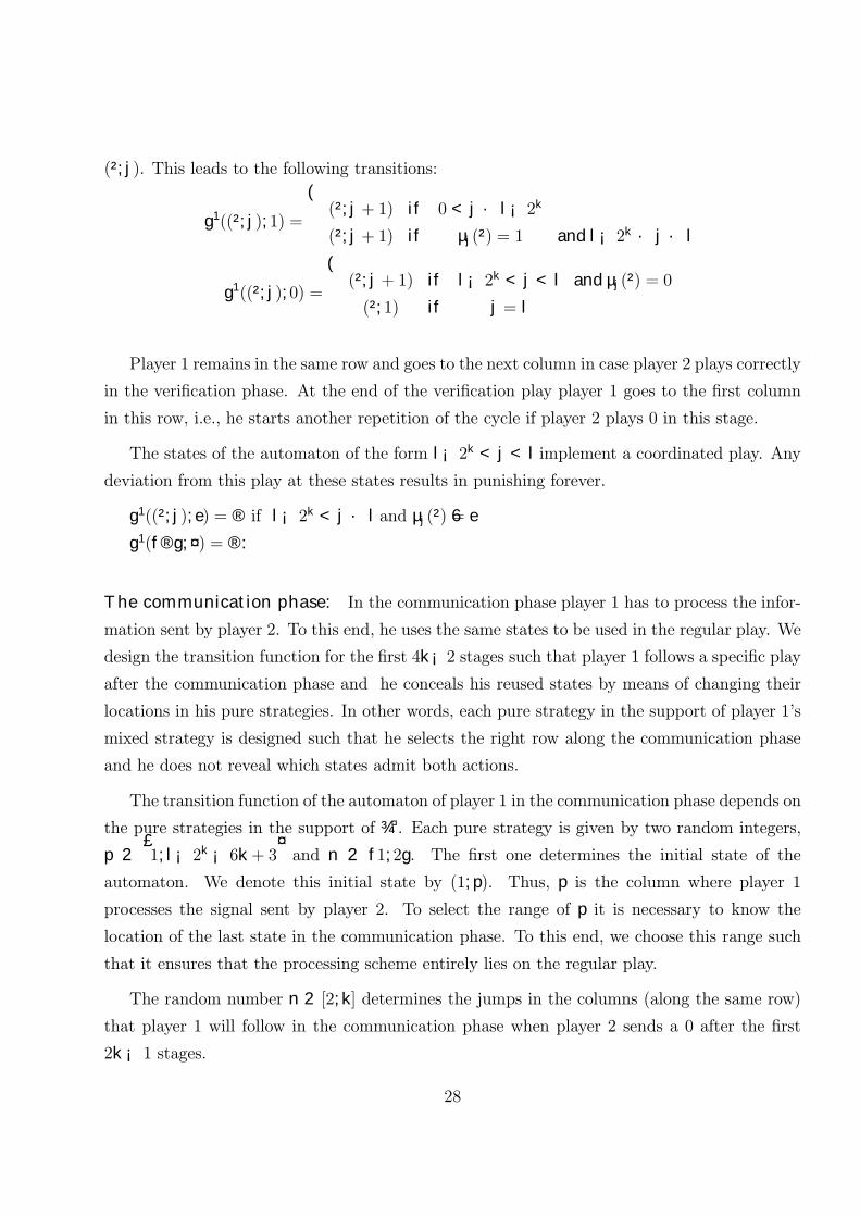
Figure 1 illustrates the automaton of player 1 for k = 3; and j Q j= (23 ¡ 1)Á(23¡1)3

= 762= 14: Suppose that the regular play has 12 columns and that the veri¯cation play has 23 = 8

associated columns. The ¯lled disks (²) represent states of the automaton whose action functionis 1, "cooperate", when player 2 plays 1 as well. The small disks (±) represent states that playthe action 0, "defect", when player 2 plays 0. The big disks (°) mean the ¯nal states of theveri¯cation phase where both players have to play "defect" at the same time. The transition

function in this state goes to the ¯rst state in the same row. The horizontal arrows indicate

the transition of the automaton when player 1 follows a coordinated play.

² ! ! ² ! ± ! ± ! ² ! ± ! ² ! ² ! ² ! J0 0 1 0 1 1 1 0

² ! ! ² ! ± ! ± ! ² ! ² ! ² ! ± ! ² ! J0 0 1 1 1 0 1 0

² ! ! ² ! ± ! ² ! ± ! ± ! ² ! ² ! ² ! J0 1 0 0 1 1 1 0

² ! ! ² ! ± ! ² ! ± ! ² ! ² ! ² ! ± ! J0 1 0 1 1 1 0 0

² ! ! ² ! ± ! ² ! ² ! ² ! ± ! ² ! ± ! J0 1 1 1 0 1 0 0

² ! ! ² ! ± ! ² ! ² ! ² ! ± ! ± ! ² ! J0 1 1 1 0 0 1 0

² ! ! ² ! ² ! ² ! ² ! ± ! ± ! ² ! ± ! J1 1 1 0 0 1 0 0

² ! ! ² ! ² ! ² ! ² ! ± ! ² ! ± ! ± ! J1 1 1 0 1 0 0 0

² ! ! ² ! ² ! ² ! ± ! ± ! ² ! ± ! ² ! J1 1 0 0 1 0 1 0

² ! ! ² ! ² ! ² ! ± ! ² ! ± ! ± ! ² ! J1 1 0 1 0 0 1 0

² ! ! ² ! ² ! ± ! ² ! ² ! ² ! ± ! ± ! J1 0 1 1 1 0 0 0

² ! ! ² ! ² ! ± ! ² ! ± ! ± ! ² ! ² ! J1 0 1 0 0 1 1 0

² ! ! ² ! ² ! ± ! ± ! ² ! ± ! ² ! ² ! J1 0 0 1 0 1 1 0

² ! ! ² ! ² ! ± ! ± ! ² ! ² ! ² ! ± ! J1 0 0 1 1 1 0 0

Veri¯cation PlayRegular Play

Figure 1.

The transitions of the automaton will be de¯ned such that for each ¯xed ² 2 Q, if player

2's strategy is ¿ ², the state of the automaton at stage t = jmod(l + 4k ¡ 2) with 0 · j · l, is

27

(²; j). This leads to the following transitions:

g1((²; j); 1) =

((²; j + 1) if 0 < j · l ¡ 2k

(²; j + 1) if µj(²) = 1 and l ¡ 2k · j · l

g1((²; j); 0) =

((²; j + 1) if l ¡ 2k < j < l and µj(²) = 0

(²; 1) if j = l

Player 1 remains in the same row and goes to the next column in case player 2 plays correctly

in the veri¯cation phase. At the end of the veri¯cation play player 1 goes to the ¯rst column

in this row, i.e., he starts another repetition of the cycle if player 2 plays 0 in this stage.

The states of the automaton of the form l ¡ 2k < j < l implement a coordinated play. Any

deviation from this play at these states results in punishing forever.

g1((²; j); e) = ® if l ¡ 2k < j · l and µj(²) 6= e

g1(f®g; ¤) = ®:

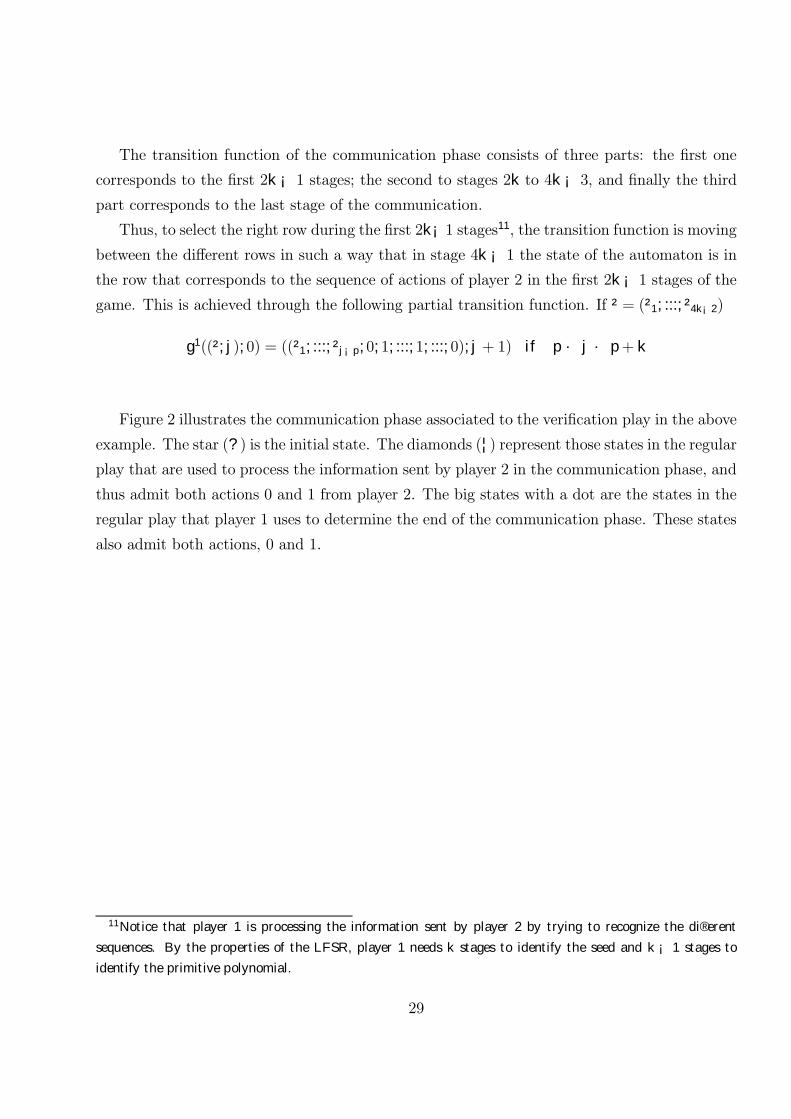
The communication phase: In the communication phase player 1 has to process the infor-

mation sent by player 2. To this end, he uses the same states to be used in the regular play. We

design the transition function for the ¯rst 4k ¡2 stages such that player 1 follows a speci¯c playafter the communication phase and he conceals his reused states by means of changing their

locations in his pure strategies. In other words, each pure strategy in the support of player 1's

mixed strategy is designed such that he selects the right row along the communication phase

and he does not reveal which states admit both actions.

The transition function of the automaton of player 1 in the communication phase depends on

the pure strategies in the support of ¾¤. Each pure strategy is given by two random integers,

p 2 £1; l ¡ 2k ¡ 6k + 3¤ and n 2 f1; 2g. The ¯rst one determines the initial state of the

automaton. We denote this initial state by (1; p). Thus, p is the column where player 1

processes the signal sent by player 2. To select the range of p it is necessary to know the

location of the last state in the communication phase. To this end, we choose this range such

that it ensures that the processing scheme entirely lies on the regular play.

The random number n 2 [2; k] determines the jumps in the columns (along the same row)

that player 1 will follow in the communication phase when player 2 sends a 0 after the ¯rst

2k ¡ 1 stages.

28

The transition function of the communication phase consists of three parts: the ¯rst one

corresponds to the ¯rst 2k ¡ 1 stages; the second to stages 2k to 4k ¡ 3, and ¯nally the third

part corresponds to the last stage of the communication.

Thus, to select the right row during the ¯rst 2k¡1 stages11, the transition function is moving

between the di®erent rows in such a way that in stage 4k ¡ 1 the state of the automaton is inthe row that corresponds to the sequence of actions of player 2 in the ¯rst 2k ¡ 1 stages of thegame. This is achieved through the following partial transition function. If ² = (²1; :::; ²4k¡2)

g1((²; j); 0) = ((²1; :::; ²j¡p; 0; 1; :::; 1; :::; 0); j + 1) if p · j · p+ k

Figure 2 illustrates the communication phase associated to the veri¯cation play in the above

example. The star (? ) is the initial state. The diamonds (¦) represent those states in the regularplay that are used to process the information sent by player 2 in the communication phase, and

thus admit both actions 0 and 1 from player 2. The big states with a dot are the states in the

regular play that player 1 uses to determine the end of the communication phase. These states

also admit both actions, 0 and 1.

11Notice that player 1 is processing the information sent by player 2 by trying to recognize the di®erent

sequences. By the properties of the LFSR, player 1 needs k stages to identify the seed and k ¡ 1 stages to

identify the primitive polynomial.

29

² ! ² ! ± ! ± ! ² ! ² ! ± ! ² ! ² ! J ! ² ! ± ! ± ! ² ! ± ! ² ! ² ! ² ! J² ! ² ! ± ! ± ! ² ! ± ! ² ! ² ! ² ! J ! ² ! ± ! ± ! ² ! ² ! ² ! ± ! ² ! J² ! ² ! ± ! ² ! ± ! ² ! ± ! ² ! ² ! J ! ² ! ± ! ² ! ± ! ± ! ² ! ² ! ² ! J² ! ² ! ± ! ² ! ± ! ± ! ² ! ² ! ² ! J ! ² ! ± ! ² ! ± ! ² ! ² ! ² ! ± ! J² ! ² ! ± ! ² ! ² ! ² ! ± ! ² ! ± ! J ! ² ! ± ! ² ! ² ! ² ! ± ! ² ! ± ! J² ! ² ! ± ! ² ! ² ! ± ! ² ! ² ! ± ! J ! ² ! ± ! ² ! ² ! ² ! ± ! ± ! ² ! J² ! ² ! ² ! ² ! ² ! ² ! ± ! ± ! ± ! J ! ² ! ² ! ² ! ² ! ± ! ± ! ² ! ± ! J² ! ² ! ² ! ² ! ² ! ± ! ² ! ± ! ± ! J ! ² ! ² ! ² ! ² ! ± ! ² ! ± ! ± ! J² ! ² ! ² ! ² ! ± ! ² ! ± ! ² ! ± ! J ! ² ! ² ! ² ! ± ! ± ! ² ! ± ! ² ! J² ! ² ! ² ! ² ! ± ! ± ! ² ! ² ! ± ! J ! ² ! ² ! ² ! ± ! ² ! ± ! ± ! ² ! J² ! ² ! ² ! ± ! ² ! ² ! ± ! ² ! ± ! J ! ² ! ² ! ± ! ² ! ² ! ² ! ± ! ± ! J² ! ² ! ² ! ± ! ² ! ± ! ² ! ² ! ± ! J ! ² ! ² ! ± ! ² ! ± ! ± ! ² ! ² ! J² ! ² ! ² ! ± ! ± ! ² ! ± ! ² ! ² ! J ! ² ! ² ! ± ! ± ! ² ! ± ! ² ! ² ! J² ! ² ! ² ! ± ! ± ! ± ! ² ! ² ! ² ! J ! ² ! ² ! ± ! ± ! ² ! ² ! ² ! ± ! J

Veri¯cation PlayRegular Play

Figure 2.

In second place, we design the transition function12 when player 2 is sending the last part

of the seed but the last stage, i.e., for t : 4k ¡ 2 > t > 2k ¡ 1. Here, the randomness of the

jumps allow player 1 to hide the reused states.

As we noted above, player 1's automaton is a matrix with l columns and 2k(Á(2k¡1)k

) rows,

i.e., 2k( 2k¡1k log k

) rows. The communication phase starts in the p column that player 1 has chosen

randomly. Hence, the states used to process the seed are located in a submatrix with 4k ¡ 2

rows and a number of columns which depends on n.

Now, the associated transition function for t : 4k ¡ 3 > t > 2k ¡ 1 is de¯ned by:

g1((²; j); 0) = (²; j + n) if p+ 2k ¡ 1 < j < p+ 4k ¡ 2 and ²j = 0

12Notice that we do not use a distribution over transition functions, but we produce enough uncertainty on

the ¯nal states of the transition function to deter deviations.

30

Finally, the last state in the communication phase is not in the same column for every row.

It depends on ²; n; p, i.e. on where the communication starts, on the distribution of ones in ²

and on the number of jumps.

This state is de¯ned as follows for every message:

Let ev be a functionev : Q ¡! [p+ k; p+ 6k ¡ 3]

² ¡! ev(²) = p+ 2k ¡ 1 + (2k ¡ 1¡ P2k¡1i=1 ²i) + n

P2k¡1i=1 ²i

Let ev be the max ev(²) where ² 2 Q:

Notice that p will be chosen13 such that [p; p+ ev] ½ £1; l ¡ 2k

¤:

The initial state is (1; p) where 1 means the signal whose ¯rst 2k ¡ 1 components are onesand p is a random value such that [p; p+ ev] ½ £

1; l ¡ 2k¤that player 1 chooses.

Now it is possible to de¯ne the transition function for the ¯nal state for every row: g1((²; ev(²)); 0) =(²; 1):

This is equivalent to: g1((1; p); ²) = (²; 1):

In all other cases the value of g1 equals ®.

Figure 3 illustrates14 the scheme that player 1 follows to process the message sent by player

2. This is an example for k = 3; p = 5 and n = 2: The star (? ) represents the initial state of

the automaton of player 1.

13Notice that this set is not empty, since T ¡ L TL+± < l ¡ s:

14We consider the primitive polynomial f(x) = x4 + x + 1 on GF(2):

31

² ! ² ! ² ! ² ! ² ! ² ! J0 0 1 0 1 1 1 0

² ! ² ! ¦ ! ¦ ! ² ! ² ! ² ! J0 0 1 1 0 1 1 0

² ! ² ! ² ! ² ! ² ! ² ! J0 1 0 0 1 1 1 0

² ! ² ! ¦ ! ¦ ! ² ! ² ! ² ! J0 1 0 1 0 1 1 0

² ! ² ! ² ! ² ! ² ! ¦ ! ² ! J0 1 1 0 1 1 0 0

¦ ! ¦ ! ¦ ! ¦ ! ² ! ² ! ¦ ! ² ! J0 1 1 1 0 1 0 0

¤ ! ¦ ! ¦ ! ¦ ! ¦ ! ² ! ¦ ! ² ! ¦ ! ² ! J1 1 1 1 0 0 0 0

² ! ² ! ² ! ² ! ¦ ! ² ! ¦ ! ² ! J1 1 1 0 1 0 0 0

² ! ² ! ¦ ! ¦ ! ² ! ² ! ¦ ! ² ! J1 1 0 1 0 1 0 0

² ! ² ! ² ! ² ! ² ! ¦ ! ² ! J1 1 0 0 1 1 0 0

² ! ¦ ! ¦ ! ² ! ² ! ¦ ! ² ! J1 0 1 1 1 1 0 0

² ! ² ! ² ! ² ! ² ! ¦ ! ² ! J1 0 1 0 1 1 0 0

² ! ² ! ¦ ! ¦ ! ² ! ² ! ² ! J1 0 0 1 0 1 1 0

² ! ² ! ² ! ² ! ² ! ² ! J1 0 0 0 1 1 1 0

@@R

@@R

@@R

@@R

¡¡µ

¡¡µ

¡¡µ

¡¡µ

¢¢¢¢̧

¢¢¢¢̧

AAAAU

£££££££±

BBBBBBBN ?

?

?

?

?

?

?

?

?

?

?

?

?

?

?

?

?

Figure 3: Communication phase.

6.8 Equilibrium conditions:

We check here that the constructed strategies are indeed an equilibrium. We show ¯rst that

any pro¯table deviation by player 1, cannot be implemented by a ¯nite automata of complexity

m1: Then, we study the complexity of a strategy of player 1 which yields a higher payo® when

playing against ¿ ¤, i.e. comp1(¾) where r1T (¾; ¿¤) ¸ PT

t=1r1(!(²))

T: Secondly, we show that with

probability close to 1 there is no pro¯table deviation by player 2.

Let ¾ be a strategy of player 1 and ² 2 Q, with r1T (¾; ¿ ²) ¸ PT

t=1r1(!(²))

T: Then, !t(¾; ¿ ²) =

!(²) for any t · Tzwhere z is a ¯xed number that depends on the action pair (1,1), with

payo®s (3; 3), and on the other payo®s of the stage game PD (4 and 1 in our model). Note

that z < 1; 5. Therefore, for any strategy ¾ of player 1, r1T (¾; ¿ ²) · PT

t=1r1(!(²))

T+ C

Twhere

C ¸ T (4¡ 3 + ").

32

Let ¾ be a pure strategy for player 1 with r1T (¾; ¿¤) ¸ PT

t=1r1(!(²))

Tand such that ¾ is

implemented by an automaton of size m1.

In order to characterize the size of the automaton which implements a pro¯table deviation,

consider the following partition of the set of seeds

Let

Q(1; ¾) =n

² 2 Q such that r1T (¾; ¿ ²) >

PTt=1

r1(!(²))T

oQ(2; ¾) =

n² 2 Q such that r1

T (¾; ¿ ²) =PT

t=1r1(!(²))

T

oQ(3; ¾) =

n² 2 Q such that r1

T (¾; ¿ ²) <PT

t=1r1(!(²))

T

oTo study the complexity of ¾ we must know that of !(²) for every ² 2 Q, hence we analyze

the complexity for every set of the partition of Q. De¯ne Q1 = f!(¾; ¿ ²) : ² 2 Q(1; ¾)g ; Q2 =

f!(¾; ¿ ²) : ² 2 Q(2; ¾)g ; and Q3 = f!(¾; ¿ ²) : ² 2 Q(3; ¾)g : Notice that comp1(Q2) ¸ l jQ(2; ¾)jby lemma 7.

As ¾ veri¯es that r1T (¾; ¿ ¤) ¸ PT

t=1r1(!(²))

Tthen r1

T (¾; ¿ ¤) ¸ 1jQj

P²2Q

PTt=1

r1(!(²))T

: Hence,

r1T (¾; ¿¤) =

P²2Q

1jQjr

1T (¾; ¿ ²) =

1jQj

£§²2Q(1;¾)r

1T (¾; ¿ ²) + §²2Q(2;¾)r

1T (¾; ¿ ²) + §²2Q(3;¾)r

1T (¾; ¿ ²)

¤Now, since any strategy ¾ of player 1, r1

T (¾; ¿ ²) · PTt=1

r1(!(²))T

+ CTand by the de¯nition of

Q(3; ¾); then

jQ(1; ¾)j³PT

t=1r1(!(²))

T+ C

T

´+ jQ(3; ¾)j

³PTt=1

r1(!(²))T

´¸

jQ(1; ¾) +Q(3; ¾)j³PT

t=1r1(!(²))

T

´Thus C

TjQ(1; ¾)j ¸ jQ(3; ¾)j and for T large enough jQ(1; ¾)j ¸ 2 jQ(3; ¾)j

In the next lemma we study the least complexity of a strategy of player 1 which can give

him more thatPT

t=1r1(!t(²))

T.

Lemma 8 The complexity of ¾ such that r1T (¾; ¿ ¤) ¸ PT

t=1r1(!(²))

Tis

comp1(¾) ¸ 3l jQ(1; ¾)j+ l jQ(2; ¾)j

Proof:

By the de¯nition of complexity, comp1(¾) = comp1 f!(¾; ¿ ²) : ² 2 Qg ¸comp1 f!(¾; ¿ ²) : ² 2 Q(1; ¾) [ Q(2; ¾)g =

33

comp1(Q1) + comp1(Q2):

Notice that comp1(Q2) ¸ l jQ(2; ¾)j by lemma 7. Let us bound the complexity of Q1:

By the de¯nition of Q(1; ¾), for every ² 2 Q(1; ¾), r1T (¾; ¿ ²) > R1(!(²)): Therefore there

exists a deviation from the proposed play at the end of the game i.e., for every t · 2k + 4l;

!t(¾; ¿ ²) = !t(²): Now by lemma 4, a deviation after 4k ¡ 2 + 4l stages entails a complexity ofplayer 1 of at least 3l. By the de¯nition of complexity with ¯nite automata it is su±cient to

prove that for every pair (²; t); (²0; t0) with (²; t) 6= (²0; t0) and t ¸ t0 in

Q(1; ¾)£ f4k ¡ 2 + 1; :::; 4k ¡ 2 + 3lg

there exists s < T ¡ t such that

(!2t (²); :::; !2

t+s(²)) = (!2t0(²0); :::; !2

t0+s(²0))

and

¾(!1(²); ::; !t+s(²)) 6= ¾(!1(²0); ::; !t0+s(²¶))

We just consider the case where t 6= t. (The other case satis¯es the condition of lemma 7).

We suppose now that t > t0; t = t0 mod (l) and ² 2 Q(1; ¾):

Let s be the largest positive integer such that

!t(²); :::; !t+s(²) = !t0(¾; ¿ ²); :::; !t0+s(¾; ¿ ²):

As r1T (¾; ¿ ²) ¸ PT

t=1r1(!(²))

T) s < T ¡ t and

¾(!t(²); :::; !t+s(²)) 6= ¾(!t0(²0); :::; !t0+s(²0): ¤

Lemma 9 below asserts that for any pure strategy of player 1 that play against the mixed

strategy ¿ ¤ of player 2, the payo® is the average on Q.

Lemma 9 For any strategy ¾ 2 §1(m1)

r1T (¾; ¿¤) · 1

jQjP

Q R1(!(²))

Proof:

Suppose that r1T (¾; ¿¤) ¸ PT

t=1r1(!(²))

T:

Consider the partition of Q = Q(1; ¾) [ Q(2; ¾) [ Q(3; ¾):

First, if jQ(3; ¾)j = ; then jQj = jQ(1; ¾)j+ jQ(2; ¾)j: By the above lemma the complexityof ¾ is greater than or equal to 3l jQ(1; ¾)j+ l jQ(2; ¾)j :

34

As m1 ¸ 3ljQ(1; ¾)j+ ljQ(2; ¾)j = ljQj+ 2ljQ(1; ¾)j and since 2k¡1 · £m1¡l

l

¤< 2k; then

m1 ¸ m1 ¡ 2l + 2ljQ(1; ¾)j , jQ(1; ¾)j = ;We conclude that r1

T (¾; ¿¤) · PTt=1

r1(!(²))T

:

Next, if jQ(3; ¾)j 6= ;; as already noted, we can suppose that for T large enough jQ(1; ¾)j ¸2 jQ(3; ¾)j. Then,

m1 ¸ 3ljQ(1; ¾)j+ ljQ(2; ¾)j == l

2jQ(1; ¾)j+ 3l

2jQ(1; ¾)j+ ljQ(2; ¾)j >

> ljQj+ 52ljQ(1; ¾)j > m1: By the same argument, we get a contradiction. ¤

To conclude that (¾¤; ¿¤) is equilibrium, the next lemma states the equilibrium condition

for player 2. It is enough to prove the condition with one strategy in the support of the mixed

strategy of player 2.

Lemma 10 For any strategy ¿ 2 §2 and every ² 2 QPTt=1 r2(¾¤; ¿ ) · PT

t=1 r2(¾¤; ¿ ²):

Proof:

Let ¿ be a pure strategy of player 2 such that for some ² 2 Q, !t(¾¤; ¿ ) = !t(²) for every

1 · t · 4k ¡ 2 and r2(¾¤; ¿ ) ¸ r2(¾; ¿ ²).

Let s0 be the smallest integer that 2k < s0 · T with !s(¾¤; ¿ ) 6= !s0(²) and !t(¾

¤; ¿ ) =

!t(²) 1 < t < s0.

Let ev = max fev(²) such that ² 2 QgObserve that T ¡ 4k ¡ 2¡ Ll is of the order ±l and for su±ciently large values of T; these

stages !t(²) = (1; 1) for T > t > p + ev + 4k ¡ 2 + Ll. Hence, any strategy ¾ in the support of

¾¤does not tolerate any deviation from the proposed play for T > t > p+ ev + 4k ¡ 2 + Ll and

r2(1; b2) ¸ r2(1; 1) > u2(PD).

Therefore, if T > s > 4k¡2+Ll+p+ev then the strategy ¾¤ does not tolerate any deviation.

Hence, r2(¾¤; ¿ ) < r2(¾¤; ¿ ²), and if s = T then r2(¾¤; ¿ ) < r2(¾¤; ¿ ²).

If 2k < s < 2k + Ll + p + ev then with probability close to one the strategy of player 1, ¾¤;

detects the deviation of player 2 in future stages and player 1 punishes forever. Notice that

player 2 gains more if he deviates at the end of the game. The other deviations are punishable

with probability close to one:

35

If player 2 deviates in the communication phase, i.e.: if (!21(¾

¤; ¿ ); :::; !22k(¾

¤; ¿)) is not in

Q, then with probability at least 12player 1 will detect the deviation before l stages. Player 2

loses T ¡lT(x2 ¡ u2) against what he may win, 2k¡1

T.

Therefore ¿¤ is a best reply against ¾¤. ¤

36

7 Concluding Remarks

The design of optimal communication schemes is important when communication is inter-play

and games are repeated a ¯nite number of times. When players implement their strategies

by means of ¯nite automata these communication schemes may also determine the number of

possible plays to achieve a cooperative outcome.

We have presented an equilibrium construction with an optimal communication scheme. Our

equilibrium condition in terms of the upper bound of the smallest automaton implementing the

cooperative outcome and which depends on both the "¡approximation to the e±cient outcomeand the number T of repetitions, lies between that of PY (1994) and the one of N (1998).

Namely, our upper bound includes that of PY (1994), but, in turn, it is included in the one

of N (1998). The reason behind this last relationship between Neyman's upper bound and

ours is that the Prisoner's Dilemma game does not belong to the class of games where the

communication phase dictates the "¡approximation to the e±cient outcome.In the class of games where this distortion rate is only generated by the communication

process, the optimality of such a process is vital for the equilibrium conditions. For instance,

and without loss of generality, suppose a 2 player game where the targeted cooperative payo®

belongs to the convex hull of the two actions a11 and a1

2 of player 1 and a21 and a2

2, of player

2, i.e., x = ¸1r(a11; a2

1) + ¸2(a12; a2

2), with ¸i > 0; i = 1; 2 andP

i=1;2 ¸i = 1: Label a11 and

a21 by 0 and a1

2 and a22 by 1, then x = ¸1r(0; 0) + ¸2(1; 1): Following our approach, and for T

large enough, the equilibrium play consists of a communication phase, which is composed of

the actions pairs (0; 0) and (0; 1), and a cycle play, where the action pairs (0; 0) and (1; 1) are

played in both the regular and the veri¯cation plays. In this case, the "-approximation to x

only depends on the (2k ¡ 1) stages of the communication phase where the action pair (0; 1) isplayed.

Known results in the automata complexity's literature (see Neyman, 1998) state that the

upper bounds of the automata have to be subexponential to achieve cooperation in ¯nite

repetition of the underlying game. In the above problem, the upper bound of player 1 is lower

than exp( "Tc), where c is a parameter which depends on the speci¯c game's payo®s. Our bound

is the largest bound to achieve cooperation in a ¯nitely repeated game played by ¯nite automata

and it improves all the other bounds already o®ered in the ¯eld. This improvement is due to

our optimal codi¯cation of the communication phase.

37

8 REFERENCES

Gossner, O. (2000): "Sharing a long secret in a few public words", Working Paper 2000-15,

THEMA, UMER CNRS.

Hardly, G.H. and Wright, E.M (1980).: An Introduction to the Theory of Numbers., Oxford

University Press, Oxford.

Kalai, E. (1990): "Bounded rationality and strategic complexity in repeated games",.T.

Ichiishi, A. Neyman, Y. Tauman, eds., Game Theory and Applications, Academic Press, New

York, 131-157.

Kalai, E, and Standford,W (1988): "Finite Rationality and Interpersonal Complexity in

Repeated Games", Econometrica 56, 2, 397-410.

Nidl and Niederreiter.(1983): Finite Fields. Encyclopedia of Mathematics and its Applica-

tions, Gian-Carlo Rota, editor. Cambridge. Massachusetts.

Neyman, A. (1985): "Bounded complexity justi¯es cooperation in the ¯nitely repeated

prisoner's dilemma", Economics Letters 19, 227-229.

|||| (1997): "Cooperation, repetition, and automata", S. Hart, A. Mas Colell, eds.,

Cooperation: Game-Theoretic Approaches, NATO ASI Series F, 155. Springer-Verlag, 233-255.

|||| (1998): "Finitely Repeated Games with Finite Automata", Mathematics of Op-

erations Research 23, 3, 513-552.

Rubinstein,A (1986): "Finite Automata play the repeated prisoners' dilemma", Journal of

Economic Theory 39, 83-96.

Shannon, C.E. (1948): "A Mathematical Theory of Communication", Bell System Tech. J.

27, 379-423 and 623-656.

Zemel, E. (1989): "Small talk and cooperation: A note on bounded rationality", Journal of

Economic Theory 49, 1, 1-9.

38