Commun Nonlinear Sci Numer Simulat 61 (2018) 149–159

Contents lists available at ScienceDirect

Commun Nonlinear Sci Numer Simulat

journal homepage: www.elsevier.com/locate/cnsns

Research paper

A benchmark problem for the two- and three-dimensional

Cahn–Hilliard equations

Darae Jeong, Yongho Choi, Junseok Kim

∗

Department of Mathematics, Korea University, Seoul 02841, Republic of Korea

a r t i c l e i n f o

Article history:

Received 20 May 2017

Revised 21 December 2017

Accepted 6 February 2018

Available online 8 February 2018

Keywords:

Cahn–Hilliard equation

Finite difference method

Multigrid method

Benchmark problem

a b s t r a c t

This paper proposes a benchmark problem for the two- and three-dimensional Cahn–

Hilliard (CH) equations, which describe the process of phase separation. The CH equation

is highly nonlinear and an analytical solution does not exist except trivial solutions. There-

fore, we have to approximate the CH equation numerically. To test the accuracy of a nu-

merical scheme, we have to resort to convergence tests, which consist of consecutive rela-

tive errors or a very fine solution from the numerical scheme. For a fair convergence test,

we provide benchmark problems which are of the shrinking annulus and spherical shell

type. We show numerical results by using the explicit Euler’s scheme with a very fine

time step size and also present a comparison test with Eyre’s convex splitting schemes.

© 2018 Elsevier B.V. All rights reserved.

1. Introduction

This paper proposes a benchmark problem for the two- and three-dimensional Cahn–Hilliard (CH) equations, which were

originally introduced as a mathematical model of phase separation in a binary alloy [1,2] :

∂φ( x , t)

∂t = �μ(φ(x , t)) , x ∈ �, 0 < t ≤ T , (1)

μ(φ(x , t)) = F ′ (φ(x , t)) − ε2 �φ(x , t) , (2)

where � ⊂ R

d (d = 1 , 2 , or 3) is a bounded domain, F (φ) = 0 . 25(φ2 − 1) 2 , and ε is the gradient energy coefficient. The

quantity φ( x , t ) is defined as the difference of molar fractions of two species.

The CH equation has been applied to model many scientific processes such as phase separation and coarsening phenom-

ena [1,3] , image inpainting (the process of reconstructing lost or deteriorated parts of images) [4] , image segmentation [5] ,

multiphase fluid flows [6–9] , diblock copolymer (a polymer consisting of two types of monomers) [10–12] , microstructures

with elastic inhomogeneity [13,14] , topology optimization for optimizing material shape within a given design space and a

set of loads and boundary conditions [15,16] , and tumor growth simulation [17–19] . Many efficient and accurate numeri-

cal methods have been proposed to solve the CH equation. For example, the methods are meshless method [20,21] , dual

reciprocity method [22] , Galerkin method [23–25] , Fourier spectral method [26–29] , unconditionally stable scheme [30–32] ,

multigrid [16] , Crank–Nicholson method [33–35] , and Runge–Kutta method [36] .

∗ Corresponding author.

E-mail address: cfdkim@korea.ac.kr (J. Kim).

URL: http://math.korea.ac.kr/~cfdkim/ (J. Kim)

https://doi.org/10.1016/j.cnsns.2018.02.006

1007-5704/© 2018 Elsevier B.V. All rights reserved.

150 D. Jeong et al. / Commun Nonlinear Sci Numer Simulat 61 (2018) 149–159

However, the CH equation is highly nonlinear due to the term F ( φ) and an analytical solution does not exist except trivial

constant solutions. To test the accuracy of a numerical scheme for the CH equation, we have to resort to convergence tests,

which consist of consecutive relative errors or a very fine solution from the numerical scheme. The growing phase field

community has developed many numerical methods; however, the lack of benchmark problems to consistently evaluate

the numerical performance of the developed code [37] has been an issue. Recently, a couple of research papers have been

published that are related to benchmark problems. In [38] , the author has derived analytical expressions for the solution

of a surface Hele–Shaw model on the sphere, to serve numerical purposes, as a benchmark for the surface CH equation. In

[37] , the authors presented two benchmark problems for the numerical implementation of phase field equations that model

solute diffusion along with second phase growth and coarsening.

The main purpose of this paper is to present benchmark problems for testing numerical schemes for the CH equations.

The two benchmark problems are of the shrinking annulus and spherical shell type. These benchmark problems will help

researchers in testing the accuracy of the developed computer codes for the CH equations. We give numerical results by

using the explicit Euler’s scheme with a very fine time step size and we also present a comparison test with Eyre’s con-

vex splitting schemes. This paper is organized as follows. In Section 2 , we describe the numerical solution algorithm. The

numerical results are presented in Section 3 . Some concluding remarks are presented in Section 4 .

2. Numerical solution

To obtain simple benchmark solutions, we consider the CH equation in radially (2D) as well as spherically (3D) symmetric

forms:

φt (r, t) =

1

r d−1 [ r d−1 μr (r, t)] r , r ∈ �, t > 0 , (3)

μ(r, t) = F ′ (φ(r, t)) − ε2

r d−1 [ r d−1 φr (r, t)] r , (4)

where d is the space dimension. Here, we use the homogeneous Neumann boundary conditions for both φ and μ. Note

that Eqs. (3) and (4) represent the radially and spherically symmetric CH equations when d = 2 and d = 3 , respectively. The

derivation of Eqs. (3) and (4) is described below for more detail.

• The two-dimensional Cartesian coordinate can be represented by the polar coordinate as (x, y ) = (r cos θ, r sin θ ) . In the

two-dimensional polar coordinate, Eqs. (1) and (2) become

∂φ(r, θ, t)

∂t =

1

r

∂

∂r

(r ∂μ

∂r

)+

1

r 2 ∂ 2 μ

∂θ2 ,

μ(r, θ, t) = F ′ (φ) − ε2

r

∂

∂r

(r ∂φ

∂r

)− ε2

r 2 ∂ 2 φ

∂θ2 ,

where r ≥ 0, 0 ≤ θ < 2 π , and 0 < t ≤ T . If the solutions φ and μ are radially symmetric, that is, φ = φ(r, t) and μ = μ(r, t)

are independent of θ , then

∂ 2 φ

∂θ2 =

∂ 2 μ

∂θ2 = 0 . Therefore, we can obtain Eqs. (3) and (4) when d = 2 .

• In spherical polar coordinate, (x, y, z) = (r sin θ cos ψ, r sin θ sin ψ, r cos θ ) , Eqs. (1) and (2) become

∂φ(r, θ, ψ, t)

∂t =

1

r 2 ∂

∂r

(r 2

∂μ

∂r

)+

1

r 2 sin

2 θ

[sin θ

∂

∂θ

(sin θ

∂μ

∂θ

)+

∂ 2 μ

∂ψ

2

],

μ(r, θ, ψ, t) = F ′ (φ) − ε2

r 2 ∂

∂r

(r 2

∂φ

∂r

)

− ε2

r 2 sin

2 θ

[sin θ

∂

∂θ

(sin θ

∂φ

∂θ

)+

∂ 2 φ

∂ψ

2

],

where r ≥ 0, 0 ≤ θ ≤π , 0 ≤ψ < 2 π , and 0 < t ≤ T . Likewise, if φ = φ(r, t) and μ = μ(r, t) are independent of θ and ψ , that

is, spherically symmetric, then we have Eqs. (3) and (4) when d = 3 .

Now, we solve the CH Eqs. (3) and (4) in � = (0 , 1) . Let N r be a positive integer and h = 1 /N r be the uniform grid

size. Let φn i

and μn i

be approximations of φ( r i , t n ) and μ( r i , t n ), respectively. Here, r i = (i − 0 . 5) h and t n = n �t . Then, we

discretize Eqs. (3) and (4) in time, using the explicit Euler’s method:

φn +1 i

− φn i

�t = �r μ

n i , for i = 1 , . . . , N r , (5)

μn = (φn ) 3 − φn − ε2 �r φn . (6)

i i i i

D. Jeong et al. / Commun Nonlinear Sci Numer Simulat 61 (2018) 149–159 151

Fig. 1. Schematic illustration of discrete Laplace stencil, Eq. (7) .

Here, �r denotes the discrete Laplace operator in radially and spherically symmetric coordinates. In this study, we use the

following standard discrete Laplace stencil [39] :

�r μn i =

1

r d−1 i

[r d−1

i +1 / 2

(μn

i +1 − μn

i

h

)− r d−1

i −1 / 2

(μn

i − μn

i −1

h

)]/

h, (7)

where r d−1 i +1 / 2

= (r d−1 i

+ r d−1 i +1

) / 2 . See Fig. 1 for a schematic illustration.

Also, the boundary condition is defined as φn 0

= φn 1 , φn

N r +1 = φn

N r , μn

0 = μn

1 , and μn

N r +1 = μn

N r for all n . Note that the

numerical solution from Eqs. (5) to (6) satisfy total mass conservation, that is, ∑ N r

i =1 2(d − 1) π(r i h )

d−1 φn +1 i

=

∑ N r i =1

2(d −1) π(r i h )

d−1 φn i

for all n . We can show this property as follows: By multiplying both sides in Eq. (5) with 2(d − 1) π(r i h ) d−1

and summing this with respect to i , we obtain

N r ∑

i =1

φn +1 i

− φn i

�t (r i h ) d−1 =

N r ∑

i =1

h

d−3 [r d−1

i +1 / 2 (μn +1

i +1 − μn +1

i ) − r d−1

i −1 / 2 (μn +1

i − μn +1

i −1 ) ]

= h

d−3 [r d−1

N r +1 / 2 (μn +1 N r +1 − μn +1

N r ) − r d−1

1 / 2 (μn +1 1 − μn +1

0 ) ]

= 0 ,

where the homogeneous Neumann boundary condition is used. Therefore, we can see the total mass conservation property

of the numerical solution.

3. Numerical results

3.1. Benchmark problems

In this section, we provide the benchmark problems for the CH equations. We use the following simulation parameters,

N r = 64 , h = 1 /N r , and �t = 10 h 4 . In this study, we consider the fourth order nonlinear CH equation with the explicit Euler’s

method, which is conditionally stable [40] . With the following parameters ε8 and h = 1 / 64 on � = (0 , 1) , we found that

the stable time steps are restricted by �t ≤ 120 h 4 . Therefore, for the accuracy reason, we use a small enough time step size,

�t = 10 h 4 , for the stable benchmark solution.

The initial state is assumed to be

φ(r, 0) = tanh

(0 . 1 − | r − 0 . 75 | √

2 ε

), (8)

where ε = 8 h/ [2 √

2 tanh

−1 (0 . 9)] ≈ 0 . 030019 is assumed and its value implies that we have approximately 8 grid spacing

across interfacial transition layer [41] . Unless otherwise specified, we will use this value throughout this paper.

3.1.1. Radially symmetric CH equation

First, we consider Eqs. (5) and (6) with an initial annulus shape in the two-dimensional space, i.e., d = 2 .

Fig. 2 (a) shows the temporal evolution of the phase-field φ( r, t ) up to T = 4 , 0 0 0 , 0 0 0�t . As time goes by, we can observe

that phase moves radially inward.

Here, we define the two positions, R 1 and R 2 ( R 1 > R 2 ), which satisfy φ(R 1 , t) = φ(R 2 , t) = 0 as shown in Fig. 3 . Then, we

call R 1 and R 2 the outer and inner radii, respectively.

To find R 1 and R 2 values, we first find two indices m 1 and m 2 ( m 1 > m 2 ) which satisfy φn m 1

φn m 1 +1

≤ 0 and φn m 2

φn m 2 +1

≤ 0 .

And then define outer and inner radii R 1 = r m 1 − hφm 1

/ (φm 1 +1 − φm 1 ) and R 2 = r m 2

− hφm 2 / (φm 2 +1 − φm 2

) using the linear

interpolation (see Fig. 3 ).

In Fig. 2 (b), we can observe the temporal evolution of the radii of an annulus shape up to time T . As annulus shrinks, its

corresponding radii decrease.

152 D. Jeong et al. / Commun Nonlinear Sci Numer Simulat 61 (2018) 149–159

Fig. 2. Temporal evolution of (a) the phase-field φ and (b) the radii, R 1 and R 2 , of an annulus shape.

Fig. 3. Schematic illustration of the outer and inner radii R 1 and R 2 such that φ(R 1 ) = φ(R 2 ) ≈ 0 .

Table 1

Numerical solution φ at T = 4 , 0 0 0 , 0 0 0�t ≈ 2 . 384185791015625 .

φ1 = −1 . 027504511776 φ17 = −0 . 564487217154 φ33 = 0 . 988605076047 φ49 = −0 . 983853795737

φ2 = −1 . 027498725129 φ18 = −0 . 250859935848 φ34 = 0 . 976057569899 φ50 = −0 . 985170594999

φ3 = −1 . 027484177921 φ19 = 0 . 121508898697 φ35 = 0 . 949235589084 φ51 = −0 . 985815573656

φ4 = −1 . 027453469700 φ20 = 0 . 456286812712 φ36 = 0 . 894926141320 φ52 = −0 . 986132065568

φ5 = −1 . 027391123778 φ21 = 0 . 691564085583 φ37 = 0 . 790535176743 φ53 = −0 . 986287947498

φ6 = −1 . 027265860219 φ22 = 0 . 831789202458 φ38 = 0 . 604972051322 φ54 = −0 . 986365246130

φ7 = −1 . 027014786075 φ23 = 0 . 908171459654 φ39 = 0 . 316298793368 φ55 = −0 . 986404031941

φ8 = −1 . 026511266173 φ24 = 0 . 948229985036 φ40 = −0 . 047136487092 φ56 = −0 . 986423880370

φ9 = −1 . 025499705042 φ25 = 0 . 969213404538 φ41 = −0 . 395381379124 φ57 = −0 . 986434356499

φ10 = −1 . 023463352746 φ26 = 0 . 980539743388 φ42 = −0 . 652635247975 φ58 = −0 . 986440135808

φ11 = −1 . 019357592452 φ27 = 0 . 987023989568 φ43 = −0 . 810416052062 φ59 = −0 . 986443505066

φ12 = −1 . 011078093531 φ28 = 0 . 991025054790 φ44 = −0 . 897085623619 φ60 = −0 . 986445583798

φ13 = −0 . 994428189172 φ29 = 0 . 993620193637 φ45 = −0 . 941962689380 φ61 = −0 . 986446920884

φ14 = −0 . 961230919942 φ30 = 0 . 995170132055 φ46 = −0 . 964512120376 φ62 = −0 . 986447785876

φ15 = −0 . 896344006399 φ31 = 0 . 995516163527 φ47 = −0 . 975676021778 φ63 = −0 . 986448311013

φ16 = −0 . 774692830013 φ32 = 0 . 993904512330 φ48 = −0 . 981164203364 φ64 = −0 . 986448559944

As a reference, we present the numerical solution at T = 4 , 0 0 0 , 0 0 0�t ≈ 2.384185791015625 in Table 1 . Here, we list the

numerical solution φi at each grid point r i . In addition, Table 2 shows the outer radius R 1 and the inner radius R 2 of the

annulus shape at T = t n = n �t .

3.1.2. Spherically symmetric CH equation

Next, we consider Eqs. (5) and (6) with a initial spherical shell in the three-dimensional space, i.e., d = 3 .

D. Jeong et al. / Commun Nonlinear Sci Numer Simulat 61 (2018) 149–159 153

Table 2

Outer radius R 1 and inner radius R 2 of the annulus shape at time t n .

n R 1 R 2 n R 1 R 2

0 0.84 994 9775928 0.650050224072 2 , 200 , 000 0.715853459661 0.461200493142

20 0 , 0 0 0 0.836608652655 0.631005604629 2 , 400 , 000 0.704210066169 0.443212910139

40 0 , 0 0 0 0.824165646808 0.614467922799 2 , 600 , 000 0.692702600176 0.425020719886

60 0 , 0 0 0 0.811713839369 0.597901409161 2 , 800 , 000 0.681469817957 0.406556929895

80 0 , 0 0 0 0.799325779107 0.581260935303 3 , 0 0 0 , 0 0 0 0.670197339726 0.387714 82744 9

1 , 0 0 0 , 0 0 0 0.787091221175 0.564534192377 3 , 200 , 000 0.658933164532 0.368317756760

1 , 200 , 000 0.775077346084 0.547706818509 3 , 400 , 000 0.647888500199 0.348304709234

1 , 400 , 000 0.763046909712 0.530760837096 3 , 600 , 000 0.637011986155 0.327830429530

1 , 600 , 000 0.751022358818 0.513673213674 3 , 800 , 000 0.626025964192 0.306482326034

1 , 800 , 000 0.739121856219 0.496413671465 4 , 0 0 0 , 0 0 0 0.615160983450 0.283963854877

2 , 0 0 0 , 0 0 0 0.727474182030 0.478941455356

Fig. 4. Temporal evolution of (a) the phase-field φ and (b) the radii, R 1 and R 2 , of a spherical shell shape.

Table 3

Numerical solution φ at T = 2 , 0 0 0 , 0 0 0�t ≈ 1 . 192092895507813 .

φ1 = −1 . 06 8084 980096 φ17 = 0 . 705776144838 φ33 = 1 . 003261060134 φ49 = −0 . 860686319005

φ2 = −1 . 067949971042 φ18 = 0 . 827339820108 φ34 = 1 . 004 833794 802 φ50 = −0 . 919120188681

φ3 = −1 . 067561020556 φ19 = 0 . 894195937011 φ35 = 1 . 005960524410 φ51 = −0 . 948760758857

φ4 = −1 . 066767700322 φ20 = 0 . 930573780490 φ36 = 1 . 006316793214 φ52 = −0 . 963504268526

φ5 = −1 . 065231898221 φ21 = 0 . 950985761219 φ37 = 1 . 005234082599 φ53 = −0 . 970768441032

φ6 = −1 . 062274217729 φ22 = 0 . 963216657115 φ38 = 1 . 001352427409 φ54 = −0 . 974331498760

φ7 = −1 . 056548591713 φ23 = 0 . 971239357857 φ39 = 0 . 991934425656 φ55 = −0 . 976075644 96 8

φ8 = −1 . 045400651766 φ24 = 0 . 977039639032 φ40 = 0 . 971559832319 φ56 = −0 . 976928721304

φ9 = −1 . 023650913731 φ25 = 0 . 981606057073 φ41 = 0 . 929841374677 φ57 = −0 . 977345866119

φ10 = −0 . 981462092797 φ26 = 0 . 985435130155 φ42 = 0 . 84 8204 9664 86 φ58 = −0 . 977549846106

φ11 = −0 . 901277666631 φ27 = 0 . 988781795973 φ43 = 0 . 698177190801 φ59 = −0 . 977649593104

φ12 = −0 . 755888296946 φ28 = 0 . 991781721504 φ44 = 0 . 450466519889 φ60 = −0 . 977698353914

φ13 = −0 . 515852508923 φ29 = 0 . 994510335027 φ45 = 0 . 108434401114 φ61 = −0 . 977722144585

φ14 = −0 . 179783101083 φ30 = 0 . 997010586595 φ46 = −0 . 257726 81404 8 φ62 = −0 . 977733654081

φ15 = 0 . 18936376 834 8 φ31 = 0 . 999304601478 φ47 = −0 . 555412819598 φ63 = −0 . 977739024097

φ16 = 0 . 498347347266 φ32 = 1 . 001395588233 φ48 = −0 . 749933578888 φ64 = −0 . 977741131595

Fig. 4 (a) represents the temporal evolution of the phase-field φ( r, t ) up to T = 2 , 0 0 0 , 0 0 0�t . Also, we observe the tem-

poral evolutions of the radii R 1 and R 2 of the initial spherical shell up to time T in Fig. 4 (b).

For reference, Table 3 shows the numerical solution φi ( i = 1 , · · · , 64) at T = 2 , 0 0 0 , 0 0 0�t ≈ 1 . 192092895507813 .

Table 4 also shows the outer radius R 1 and the inner radius R 2 of the spherical shell shape at time T = t n = n �t .

3.2. Convergence test on two-dimensional space

Now, we implement the convergence test on two-dimensional space with the benchmark solution. For the numerical test,

we use the following parameters, h = 1 / 64 and �t = 10 0 , 0 0 0 h 4 × 2 −m for m = 0 , 1 , . . . , 5 . In the computational domain � =(−1 , 1) × (−1 , 1) , we define the following cell-centered point ( x i , y j ), where x i = −1 + (i − 0 . 5) h and y j = −1 + ( j − 0 . 5) h

for i, j = 1 , 2 , . . . , 128 .

154 D. Jeong et al. / Commun Nonlinear Sci Numer Simulat 61 (2018) 149–159

Table 4

Outer radius R 1 and inner radius R 2 of the spherical shell at time t n .

n R 1 R 2 n R 1 R 2

0 0.84 994 9775928 0.650050224072 1 , 100 , 000 0.749566160297 0.441094263588

10 0 , 0 0 0 0.837323694919 0.627926360803 1 , 200 , 000 0.742740402958 0.421394162858

20 0 , 0 0 0 0.826 8112894 99 0.609358492100 1 , 300 , 000 0.736207511480 0.401106 8294 86

30 0 , 0 0 0 0.81660960 0 079 0.590927146279 1 , 400 , 000 0.730154296251 0.379954281355

40 0 , 0 0 0 0.807052995185 0.572483321272 1 , 500 , 000 0.724167270531 0.358182397141

50 0 , 0 0 0 0.79767494 4 4 45 0.553956623078 1 , 600 , 000 0.718728204566 0.335027456803

60 0 , 0 0 0 0.788737081934 0.5354 828844 93 1 , 700 , 000 0.713584293866 0.310549325671

70 0 , 0 0 0 0.780245116282 0.517016467259 1 , 800 , 000 0.708565628611 0.283686304333

80 0 , 0 0 0 0.771963227501 0.4 98452156 823 1 , 900 , 000 0.704071353188 0.253694261720

90 0 , 0 0 0 0.764227811704 0.479663429112 2 , 0 0 0 , 0 0 0 0.699939662701 0.218547237985

1 , 0 0 0 , 0 0 0 0.756643381504 0.460495290928

Fig. 5. Schematic illustration of the two-dimensional Cartesian coordinate. Here, square (‘ �’) and dot (‘ · ’) symbols denote benchmark solution ( φT i

) and

numerical solution ( φN t i j

), respectively.

Let φn i j

be approximations of φ( x i , y j , n �t ), where �t = T /N t is the time step, T is the final time, and N t is the total

number of time steps.

We take the following two schemes by Eyre [40,42] as test problems. One is a nonlinearly stabilized splitting scheme:

φn +1 i j

− φn i j

�t = �h μ

n +1 i j

, (9)

μn +1 i j

= F ′ (φn +1 i j

) + φn +1 i j

− φn i j − ε2 �h φ

n +1 i j

(10)

and the other is a linearly stabilized splitting scheme:

φn +1 i j

− φn i j

�t = �h μ

n +1 i j

, (11)

μn +1 i j

= F ′ (φn i j ) − 2 φn

i j + 2 φn +1 i j

− ε2 �h φn +1 i j

. (12)

Here, �h ψ i j = (ψ i −1 , j + ψ i +1 , j + ψ i, j−1 + ψ i, j+1 − 4 ψ i j ) /h 2 . We solve these discrete equations by using a full approximation

storage (FAS) multigrid method with a Gauss–Seidel relaxation [9,43,44] . The initial condition is set to be

φ(x i , y j , 0) = tanh

0 . 1 − | √

x 2 i

+ (y j − 0 . 5 h ) 2 − 0 . 75 | √

2 ε. (13)

Note that we define the initial condition as the circle with the center (0, 0.5 h ) for comparison with the benchmark solution

and the test numerical solution. See Fig. 5 .

To investigate the quantitative convergence, let us define the error of the numerical solution as e T = (e T 1 , e T 2 , · · · , e T 64 ) ,

where e T i

= φN t 64+ i, 65

− φT i

for i = 1 , 2 , · · · , 64 . Here, φN t 64+ i, 65

and φT i

denote the numerical and benchmark solutions at T =N t �t, respectively. For a better understanding, we present the schematic illustration in Fig. 5 .

Here, we consider the following discrete norm of error as

D. Jeong et al. / Commun Nonlinear Sci Numer Simulat 61 (2018) 149–159 155

Fig. 6. Columns (a)–(c) are snapshots of the numerical solutions at t = 0 , 1.311, and 2.38, respectively. The top row is a mesh view whereas the bottom

row is a filled contour at level zero.

Fig. 7. Numerical solutions using the nonlinear splitting scheme with six different time steps at T = 40 , 0 0 0 , 0 0 0 h 4 ≈ 2 . 3842 .

• the discrete l 2 -norm:

‖ e T ‖ 2 =

√

2 ( d − 1 ) π64 ∑

i =1

(e T

i

)2 ( r i )

d−1 h , (14)

• the discrete maximum norm:

‖ e T ‖ ∞

= max 1 ≤i ≤64

| e T i | , (15)

where d is the dimension of the Cartesian domain.

Fig. 6 (a)–(c) are snapshots of the numerical solutions of Eqs. (9) and (10) with �t = 3125 h 4 at t = 0 , 1.311, and 2.38,

respectively. Top row is a mesh view and bottom row is a filled contour at level zero.

Fig. 7 shows the numerical solutions using the nonlinear splitting scheme with six different time steps. We can observe

the convergence of the solutions to the benchmark solution as we refine the time step.

156 D. Jeong et al. / Commun Nonlinear Sci Numer Simulat 61 (2018) 149–159

Fig. 8. Numerical solutions using the linear splitting scheme with six different time steps at T = 40 , 0 0 0 , 0 0 0 h 4 ≈ 2 . 3842 .

Fig. 9. Temporal change of convergence rates (fifth column in Table 5 ) for numerical solution by the nonlinear scheme.

Table 5

Convergence of numerical results by the nonlinear splitting scheme with respect to time step

size �t at T = 10 0 , 0 0 0 h 4 .

Case( �t ) 25,0 0 0 h 4 Rate 12,500 h 4 Rate 6250 h 4 Rate 3125 h 4

‖ e T ‖ 2 0.006187 0.936 0.003233 1.162 0.001445 1.470 0.0 0 0521

‖ e T ‖ ∞ 0.009921 1.034 0.004844 1.368 0.001877 1.692 0.0 0 0581

Table 6

Convergence of numerical results by the linear splitting scheme with respect to time step

size �t at T = 10 0 , 0 0 0 h 4 .

Case( �t ) 25,0 0 0 h 4 Rate 12,500 h 4 Rate 6250 h 4 Rate 3125 h 4

‖ e T ‖ 2 0.010947 0.705 0.006717 0.907 0.003582 1.138 0.001628

‖ e T ‖ ∞ 0.019238 0.748 0.011455 0.958 0.005898 1.239 0.002499

Table 5 shows the discrete l 2 norm ‖ e T ‖ 2 and maximum norm ‖ e T ‖ ∞

of the errors and rates of convergence for the

results with m = 2 , 3 , 4 , 5 . This result suggests that the scheme is approximately first-order accurate in time.

Fig. 8 and Table 6 show the results using the linearly stabilized splitting scheme. The scheme also converges with ap-

proximately first-order accuracy, with though the accurate less than that of the nonlinearly stabilized splitting scheme.

If we calculate the convergence rates (the fifth column in Table 5 ) of the numerical solutions by the nonlinear scheme

for a long time, then we obtain the following results as shown in Fig. 9 . Therefore, the maximum value for the stable results

is approximately up to T = 3 .

3.3. Convergence test on three-dimensional space

As the final test, we implement a convergence test on three-dimensional space � = (−1 , 1) 3 . As in the previous sec-

tion, we define the cell-centered points ( x i , y j , z k ), where x i = −1 + (i − 0 . 5) h, y j = −1 + ( j − 0 . 5) h, and z k = −1 + (k − 0 . 5) h

for i, j, k = 1 , 2 , · · · , N x . The other numerical parameters are given as N x = 64 , h = 1 /N x , T = 20 , 0 0 0 , 0 0 0 h 4 , and �t =

D. Jeong et al. / Commun Nonlinear Sci Numer Simulat 61 (2018) 149–159 157

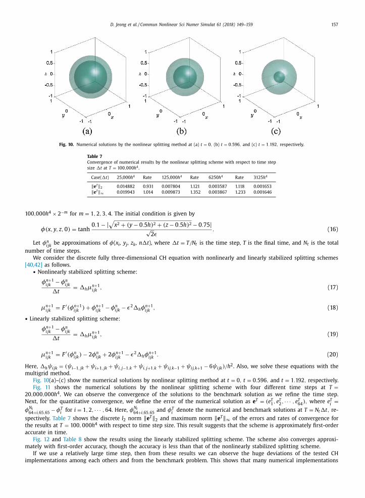
Fig. 10. Numerical solutions by the nonlinear splitting method at (a) t = 0 , (b) t = 0 . 596 , and (c) t = 1 . 192 , respectively.

Table 7

Convergence of numerical results by the nonlinear splitting scheme with respect to time step

size �t at T = 10 0 , 0 0 0 h 4 .

Case( �t ) 25,0 0 0 h 4 Rate 125,0 0 0 h 4 Rate 6250 h 4 Rate 3125 h 4

‖ e T ‖ 2 0.014882 0.931 0.007804 1.121 0.003587 1.118 0.001653

‖ e T ‖ ∞ 0.019943 1.014 0.009873 1.352 0.003867 1.233 0.001646

10 0 , 0 0 0 h 4 × 2 −m for m = 1 , 2 , 3 , 4 . The initial condition is given by

φ(x, y, z, 0) = tanh

0 . 1 − | √

x 2 + (y − 0 . 5 h ) 2 + (z − 0 . 5 h ) 2 − 0 . 75 | √

2 ε. (16)

Let φn i jk

be approximations of φ( x i , y j , z k , n �t ), where �t = T /N t is the time step, T is the final time, and N t is the total

number of time steps.

We consider the discrete fully three-dimensional CH equation with nonlinearly and linearly stabilized splitting schemes

[40,42] as follows. • Nonlinearly stabilized splitting scheme:

φn +1 i jk

− φn i jk

�t = �h μ

n +1 i jk

, (17)

μn +1 i jk

= F ′ (φn +1 i jk

) + φn +1 i jk

− φn i jk − ε2 �h φ

n +1 i jk

, (18)

• Linearly stabilized splitting scheme:

φn +1 i jk

− φn i jk

�t = �h μ

n +1 i jk

, (19)

μn +1 i jk

= F ′ (φn i jk ) − 2 φn

i jk + 2 φn +1 i jk

− ε2 �h φn +1 i jk

. (20)

Here, �h ψ i jk = (ψ i −1 , jk + ψ i +1 , jk + ψ i, j−1 ,k + ψ i, j+1 ,k + ψ i j,k −1 + ψ i j,k +1 − 6 ψ i jk ) /h 2 . Also, we solve these equations with the

multigrid method.

Fig. 10 (a)–(c) show the numerical solutions by nonlinear splitting method at t = 0 , t = 0 . 596 , and t = 1 . 192 , respectively.

Fig. 11 shows the numerical solutions by the nonlinear splitting scheme with four different time steps at T =20 , 0 0 0 , 0 0 0 h 4 . We can observe the convergence of the solutions to the benchmark solution as we refine the time step.

Next, for the quantitative convergence, we define the error of the numerical solution as e T = (e T 1 , e T

2 , · · · , e T

64 ) , where e T

i =

φN t 64+ i, 65 , 65

− φT i

for i = 1 , 2 , · · · , 64 . Here, φN t 64+ i, 65 , 65

and φT i

denote the numerical and benchmark solutions at T = N t �t, re-

spectively. Table 7 shows the discrete l 2 norm ‖ e T ‖ 2 and maximum norm ‖ e T ‖ ∞

of the errors and rates of convergence for

the results at T = 10 0 , 0 0 0 h 4 with respect to time step size. This result suggests that the scheme is approximately first-order

accurate in time.

Fig. 12 and Table 8 show the results using the linearly stabilized splitting scheme. The scheme also converges approxi-

mately with first-order accuracy, though the accuracy is less than that of the nonlinearly stabilized splitting scheme.

If we use a relatively large time step, then from these results we can observe the huge deviations of the tested CH

implementations among each others and from the benchmark problem. This shows that many numerical implementations

158 D. Jeong et al. / Commun Nonlinear Sci Numer Simulat 61 (2018) 149–159

Fig. 11. Numerical solutions using the nonlinear splitting scheme with four different time steps at T = 20 , 0 0 0 , 0 0 0 h 4 ≈ 1 . 1921 .

Fig. 12. Numerical solutions using the linear splitting scheme with four different time steps at T = 20 , 0 0 0 , 0 0 0 h 4 ≈ 1 . 1921 .

Table 8

Convergence of numerical results by the linear splitting scheme with respect to time step

size �t at T = 10 0 , 0 0 0 h 4 .

Case( �t ) 25,0 0 0 h 4 Rate 12,500 h 4 Rate 6250 h 4 Rate 3125 h 4

‖ e T ‖ 2 0.026396 0.704 0.016199 0.907 0.008638 1.114 0.003990

‖ e T ‖ ∞ 0.038912 0.729 0.023469 0.943 0.012205 1.226 0.005217

can reflect the CH equation qualitatively but not quantitatively. It also shows how important the development of benchmark

problems for the CH equation is, taking into account the large field of applications where this equation is included.

Note that we can generate other benchmark solutions with different grid sizes, initial conditions, and final times for a

benchmark problem because Eq. (6) is explicit and simple. Also note that typically, the convergence tests were performed

with a short final time.

4. Concluding remarks

In this work, we presented a benchmark problem for the two- and three-dimensional CH equations. The benchmark

problems are shrinking annulus and spherical shell domains and we obtain numerical results for the CH equation by using

the explicit Euler’s scheme with a very fine time step size. With this numerical solution we can test a temporal discretization

of the numerical scheme. As a test problem, we performed a comparison study with Eyre’s nonlinear and linear convex

splitting schemes. The computational results showed that the nonlinear convex splitting scheme is much better than the

linear one in terms of accuracy, when the time step is the same. The proposed method is general, and therefore can be

applied to other numerical schemes such as the Fourier spectral method, finite volume, and finite element method. The

proposed future work is to design a benchmark problem for a two-phase fluid flow model which consists of the Cahn–

Hilliard equation and the Navier–Stokes equation. For example, diffuse interface models for incompressible two-phase flow

with large density ratios were tested on benchmark configurations for a two-dimensional bubble rising in liquid columns

[45] .

D. Jeong et al. / Commun Nonlinear Sci Numer Simulat 61 (2018) 149–159 159

Acknowledgments

The authors thank the reviewers for the constructive and helpful comments on the revision of this article. The first

author (D. Jeong) was supported by the National Research Foundation of Korea (NRF) grant funded by the Korea government

( MSIP ) ( NRF-2017R1E1A1A03070953 ). The corresponding author (J.S. Kim) was supported by Basic Science Research Program

through the National Research Foundation of Korea(NRF) funded by the Ministry of Education ( NRF-2016R1D1A1B03933243 ).

References

[1] Cahn JW . On spinodal decomposition. Acta Metall 1961;9:795–801 . [2] Cahn JW , Hilliard JE . Free energy of a non-uniform system. I. Interfacial free energy. J Chem Phys 1958;28:258–67 .

[3] Maraldi M , Molari L , Grandi L . A unified thermodynamic framework for the modelling of diffusive and displacive phase transitions. Int J Eng Sci2012;50:31–45 .

[4] Bertozzi AL , Esedoglu S , Gillette A . Inpainting of binary images using the Cahn–Hilliard equation. IEEE T Image Process 2007;16:285–91 .

[5] Zanetti M , Ruggiero V , Miranda M Jr . Numerical minimization of a second-order functional for image segmentation. Commun Nonlinear Sci NumerSimul 2016;36:528–48 .

[6] Badalassi VE , Ceniceros HD , Banerjee S . Computation of multiphase systems with phase field models. J Comput Phys 2003;190:371–97 . [7] Heida M . On the derivation of thermodynamically consistent boundary conditions for the Cahn–Hilliard–Navier–Stokes system. Int J Eng Sci

2013;62:126–56 . [8] Kotschote M , Zacher R . Strong solutions in the dynamical theory of compressible fluid mixtures. Math Mod Meth Appl S 2015;25:1217–56 .

[9] Li Y , Choi JI , Kim J . A phase-field fluid modeling and computation with interfacial profile correction term. Commun Nonlinear Sci Numer Simul

2016;30:84–100 . [10] Choksi R , Peletier MA , Williams JF . On the phase diagram for microphase separation of diblock copolymers: an approach via a nonlocal Cahn–Hilliard

functional. SIAM J Appl Math 2009;69:1712–38 . [11] Jeong D , Lee S , Choi Y , Kim JS . Energy-minimizing wavelengths of equilibrium states for diblock copolymers in the hex-cylinder phase. Curr Appl Phys

2015;15:799–804 . [12] Jeong D , Shin J , Li Y , Choi Y , Jung J , Lee S , Kim JS . Numerical analysis of energy-minimizing wavelenghts of equilibrium states for diblock copolymers.

Curr Appl Phys 2014;14:1263–72 .

[13] Zaeem MA , Kadiri HE , Horstemeyer MF , Khafizov M , Utegulov Z . Effects of internal stresses and intermediate phases on the coarsening of coherentprecipitates: a phase-field study. Curr Appl Phys 2012;12:570–80 .

[14] Zhu J , Chen LQ , Shen J . Morphological evolution during phase separation and coarsening with strong inhomogeneous elasticity. Model Simul Mater SciEng 2001;9:499–511 .

[15] Farshbar-Shaker MH , Heinemann C . A phase field approach for optimal boundary control of damage processes in two-dimensional viscoelastic media.Math Mod Meth Appl S 2015;25:2749–93 .

[16] Zhou S , Wang M . Multimaterial structural topology optimization with a generalized Cahn–Hilliard model of multiphase transition. Struct Multidisc

Optim 2007;33:89–111 . [17] Hilforst D , Kampmann J , Nguyen TN , van der ZKG . Formal asymptotic limit of a diffuse-interface tumor-growth model. Math Mod Meth Appl S

2015;25:1011–43 . [18] Wise SM , Lowengrub JS , Frieboes HB , Cristini V . Three-dimensional multispecies nonlinear tumor growth-i: model and numerical method. J Theor Biol

2008;253:524–43 . [19] Dehghan M , Mohammadi V . Comparison between two meshless methods based on collocation technique for the numerical solution of four-species

tumor growth model. Commun Nonlinear Sci Numer Simul 2017;44:204–19 . [20] Dehghan M , Mohammadi V . The numerical solution of Cahn-Hilliard (CH) equation in one, two and three-dimensions via globally radial basis functions

(GRBFs) and RBFs-differential quadrature (RBFs-DQ) methods. Eng Anal Bound Elem 2015;51:74–100 .

[21] Dehghan M , Abbaszadeh M . The meshless local collocation method for solving multi-dimensional Cahn–Hilliard, Swift–Hohenberg and phase fieldcrystal equations. Eng Anal Bound Elem 2017;78:49–64 .

[22] Dehghan M , Mirzaei D . A numerical method based on the boundary integral equation and dual reciprocity methods for one-dimensional Cahn-Hilliardequation. Eng Anal Bound Elem 2009;33:522–8 .

[23] Elliott CM , French DA . Numerical studies of the Cahn–Hilliard equation for phase separation. IMA J Appl Math 1987;38:97–128 . [24] Gomez H , Calo VM , Bazilevs Y , Hughes TJ . Isogeometric analysis of the Cahn–Hilliard phase-field model. Comput Meth Appl Mech Eng

2008;197:4333–52 .

[25] Wells GN , Ellen K , Krishna G . A discontinuous Galerkin method for the Cahn–Hilliard equation. J Comput Phys 2006;218:860–77 . [26] He Y , Liu Y , Tang T . On large time-stepping methods for the Cahn–Hilliard equation. Appl Numer Math 2007;57:616–28 .

[27] Zhu J , Chen LQ , Shen J , Tikare V . Coarsening kinetics from a variable mobility Cahn–Hilliard equation-application of semi-implicit fourier spectralmethod. Phys Rev E 1999;60:3564–72 .

[28] Ye X , Cheng X . The fourier spectral method for the Cahn–Hilliard equation. Appl Math Comput 2005;;171:345–57 . [29] He L , Yunxian L . A class of stable spectral methods for the Cahn–Hilliard equation. J Comput Phys 2009;228:5101–10 .

[30] De Mello E , da Silveira Filho OT . Numerical study of the Cahn–Hilliard equations in one, two and three dimensions. Physica A 2005;347:429–33 .

[31] Furihata D . A stable and conservative finite difference scheme for the Cahn–Hilliard equation. Numer Math 2001;87:675–99 . [32] Zhang Z , Qiao Z . An adaptive time-stepping strategy for the Cahn–Hilliard equation. Commun Comput Phys 2012;11:1261–78 .

[33] Kim JS . A numerical method for the Cahn–Hilliard equation with a variable mobility. Commun Nonlinear Sci Numer Simul 2007;12:1560–71 . [34] Choo SM , Chung SK . Conservative nonlinear difference scheme for the Cahn–Hilliard equation. Comput Math Appl 1998;36:31–9 .

[35] Ceniceros HD , Alexandre MR . A nonstiff, adaptive mesh refinement-based method for the Cahn–Hilliard equation. J Comput Phys 2007;225:1849–62 . [36] Wodo O , Baskar G . Computationally efficient solution to the Cahn–Hilliard equation: adaptive implicit time schemes, mesh sensitivity analysis and the

3d isoperimetric problem. J Comput Phys 2011;230:6037–60 .

[37] Jokisaari AM , Voorheesa PW , Guyer JE , Warren J , Heinonen OG . Benchmark problems for numerical implementations of phase field models. CompMater Sci 2017;126:139–51 .

[38] Ratz A . A benchmark for the surface Cahn–Hilliard equation. Appl Math Lett 2016;56:65–71 . [39] Tomé MF , Castelo A , Murakami J , Cuminato JA , Minghim R , Oliveira MC , Mangiavacchi N , McKee S . Numerical simulation of axisymmetric free surface

flows. J Comput Phys 20 0 0;157:441–72 . [40] Eyre D.J.. An unconditionally stable one-step scheme for gradient systems, 1997, Preprint, http://www.math.utah.edu/ ∼eyre/research/methods/stable.ps .

[41] Choi JW , Lee HG , Jeong D , Kim JS . An unconditionally gradient stable numerical method for solving the Allen–Cahn equation. Physica A

2009;388:1791–803 . [42] Eyre DJ . Computational and mathematical models of microstructural evolution. Warrendale, PA: The Material Research Society; 1998 .

[43] Trottenberg U , Oosterlee C , Schüller A . Multigrid. London: Academic Press; 2001 . [44] Kim J , Kang K , Lowengrub J . Conservative multigrid methods for Cahn-Hilliard fluids. J Comput Phys 2004;193:511–43 .

[45] Aland S , Voigt A . Benchmark computations of diffuse interface models for two-dimensional bubble dynamics. Int J Numer Methods Fluids2012;69:747–61 .