Embed Size (px)
Citation preview
MODELING RESERVE SYSTEM
PERFORMANCE FOR LOW-DUCTILITY
BRACED FRAMES
by
MARYAM ABOOSABER
CAMERON R. BRADLEY
JESSALYN M.R. NELSON
ERIC M. HINES
Tufts University Structural Systems Communication (TUSSC)
Department of Civil and Environmental Engineering
200 College Avenue
Medford, Massachusetts 02155
Final Communication Submitted to:
the American Institute of Steel Construction
under the Contract: "Moderate Ductility Dual Systems and Reserve
Capacity"
Commucation No.
TUSSC--2011/1
December 2012


1
TABLE OF CONTENTS
LIST OF FIGURES .........................................................................................................................5
1. Introduction .............................................................................................................................9
2. SUNY Buffalo Moment Frame Test .....................................................................................14
3. One-Story System Analysis .......................................................................................................18
3.1 Scope .............................................................................................................................. 18
3.2. Ground Motions ............................................................................................................ 19
3.3 Cantilever ....................................................................................................................... 20
3.3.1. Model Setup ........................................................................................................ 20
3.3.2. Analysis Results .................................................................................................. 22
3.4 Moment Resisting Frame ............................................................................................... 25
3.4.1. Model Setup ........................................................................................................ 25
3.4.2. MRF Prototype Design ....................................................................................... 26
3.4.3. MRF Analysis Results ........................................................................................ 28
3.5 Eccentric Brace Frame ................................................................................................... 31
3.5.1. Model Setup ........................................................................................................ 31
3.5.2. Prototype Design ................................................................................................. 32
3.5.3. EBF Analysis Results ......................................................................................... 34
3.6 Low-Ductility CBF ........................................................................................................ 37

2
3.6.1. Model Setup ........................................................................................................ 37
3.6.2. Analysis Results .................................................................................................. 39
4. Nine-Story System Analysis ......................................................................................................47
4.1. Model Setup ........................................................................................................... 47
4.2. Analysis Results ..................................................................................................... 48
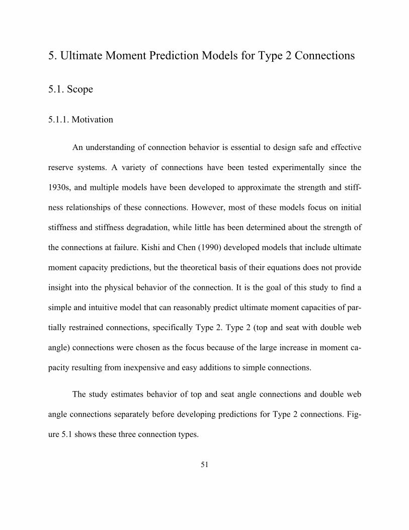
5. Ultimate Moment Prediction Models for Type 2 Connections ..................................................51
5.1. Scope ............................................................................................................................. 51
5.1.1. Motivation ........................................................................................................... 51
5.1.2. Process ................................................................................................................ 52
5.2. Top and Seat Angle Connections .................................................................................. 54
5.2.1. Chen’s Model ...................................................................................................... 55
5.2.2. Eurocode 3 Model ............................................................................................... 56
5.2.3. Simplified Model ................................................................................................ 58
5.2.4. Comparison of Models and Experimental Data .................................................. 58
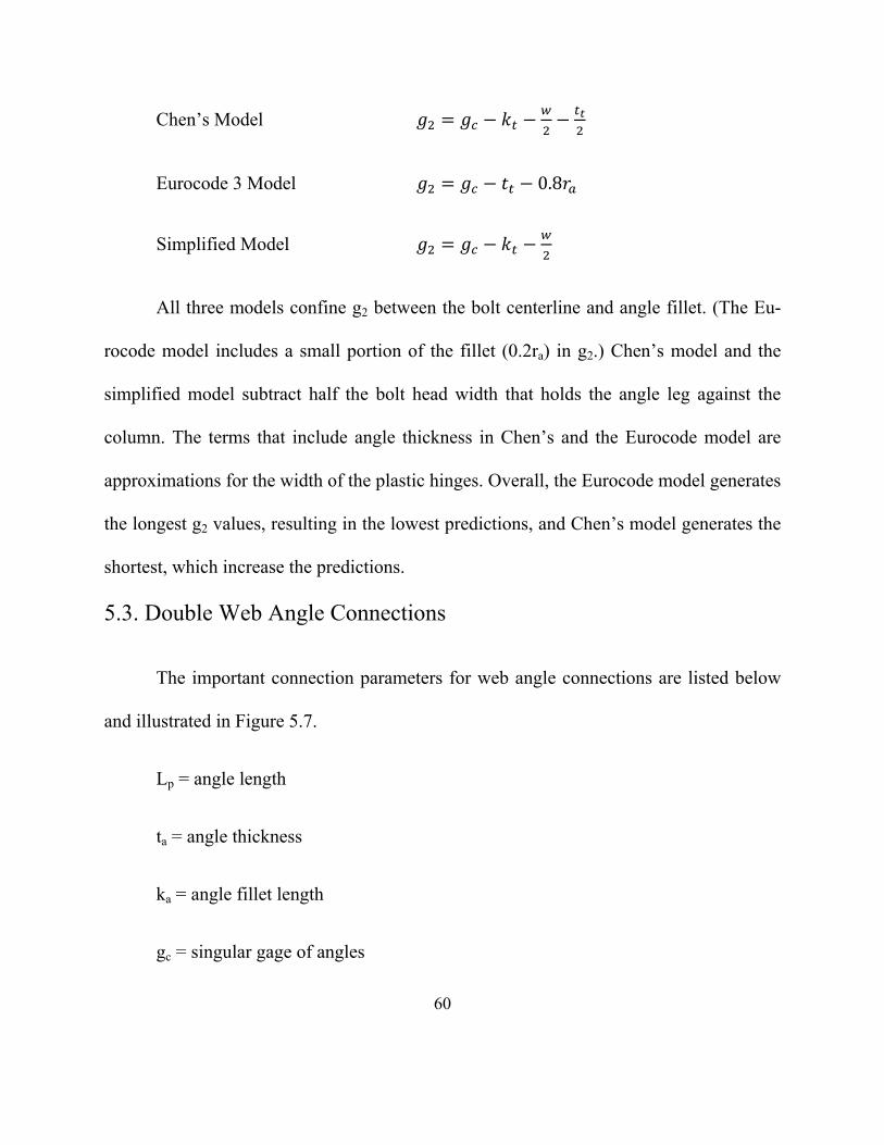
5.3. Double Web Angle Connections ................................................................................... 60
5.3.1. Chen’s Model ...................................................................................................... 62
5.3.2. Simplified Model ................................................................................................ 63
5.3.3. Comparison of Models and Experimental Data .................................................. 64
5.4. Type 2 Connections: Top and Seat Angles with Double Web Angles ......................... 65
3
5.4.1. Chen’s Model ...................................................................................................... 67
5.4.2. Simplified Model ................................................................................................ 68
5.4.3. Comparison of Models and Experimental Data .................................................. 69
5.5. Conclusions on Type 2 Study ....................................................................................... 70
6. Summary and Conclusions ........................................................................................................73
References: .....................................................................................................................................78
Appendix A ....................................................................................................................................81
A.1. Chen’s Model ............................................................................................................... 81
Example A.1 ................................................................................................................. 83
A.2. Eurocode Model ........................................................................................................... 85
Example A.2 ................................................................................................................. 87
A.3. Simplified Model .......................................................................................................... 90
Example A.3 ................................................................................................................. 92
Example A.4 ................................................................................................................. 94
Appendix B ....................................................................................................................................96
B.1. Chen’s Model ............................................................................................................... 96
Example B.1 ................................................................................................................ 100
B.2. Simplified Model ........................................................................................................ 102
Example B.2 ................................................................................................................ 104
4
Example B.3 ................................................................................................................ 105
Appendix C ..................................................................................................................................107
C.1. Chen’s Model ............................................................................................................. 107
Example C.1 ................................................................................................................ 109
C.2. Simplified Model ........................................................................................................ 112
Example C.2 ................................................................................................................ 115
Appendix D ..................................................................................................................................118

5
LIST OF FIGURES
Figure 1.1. Reserve system behavior: (a) Experimental results for the 5th Story of a 0.3 Scale, 6-
story CBF tested by Uang and Bertero (1986), as reported by Whittaker et al. (1990); (b)
Idealized system force-displacement response of a braced frame with reserve system, showing
three key parameters that affect reserve system behavior. ............................................................11
Figure 2.1. Schematic of 4-story moment frame prototype on which 1:8 scale test frame was
based. .............................................................................................................................................15
Figure 2.2: Buffalo Frame IDA Comparison (Lignos 2008, Figure 7.26). ....................................15
Figure 2.3. Buffalo Frame IDA Comparison (Experiment (NEES), Ruaumoko, OpenSees
V.2.2.0). OpenSees analysis time step differs from input time step. ............................................16
Figure 2.4. Buffalo Frame IDA Comparison (NEES, Ruaumoko, OpenSees V.2.2.0). OpenSees
analysis time step is the same as the ground motion input time step. ...........................................17
Figure 2.5. Buffalo Frame IDA Comparison (Experiment (NEES), Ruaumoko, OpenSees
V.2.2.2.e). OpenSees analysis time step is the same as the ground motion input time step .........17
Figure 3.1. Ground motions and acceleration response spectra used for this study. .....................19
Figure 3.2. Cantilever system ........................................................................................................21
Figure 3.3. Comparison of reserve system pushover curves between SDOF in Figure 4 and the
first floor reserve system for ¼ of the 9-story building .................................................................21
Figure 3.4. Cantilever IDA comparisons for GM4, GM8 and GM12 (Ruaumoko, OpenSees
V.2.2.2.e). .......................................................................................................................................22
6
Figure 3.5. Cantilever time history comparison GM8 (Ruaumoko, OpenSees V.2.2.2.e). ............23
Figure 3.5. (continued) Cantilever time history comparisons for GM8 (Ruaumoko, OpenSees
V.2.2.2.e). .......................................................................................................................................24
Figure 3.6. Moment Resisting Frame system. ...............................................................................25
Figure 3.7. CBF fracture force .......................................................................................................26
Figure 3.8. MRF moment diagram ...............................................................................................26
Figure 3.9. MRF IDA comparisons for GM4, GM8 and GM12 (Ruaumoko, OpenSees
V.2.2.2.e). .......................................................................................................................................28
Figure 3.10. MRF time history comparison GM4, GM8 and GM12 (Ruaumoko, OpenSees
V.2.2.2.e). .......................................................................................................................................29
Figure 3.10(Continue). MRF time history comparison GM4, GM8 and GM12 (Ruaumoko,
OpenSees V.2.2.2.e). ......................................................................................................................30
Figure 3.11. Eccentrically Braced Frame system. .........................................................................31
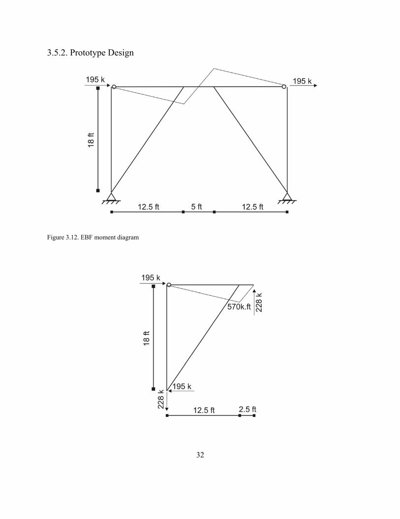
Figure 3.12. EBF moment diagram................................................................................................32
Figure 3.13. EBF IDA comparisons for GM4, GM8 and GM12 (Ruaumoko, OpenSees
V.2.2.2.e). .......................................................................................................................................35
Figure 3.14. EBF time history comparison GM8 (Ruaumoko, OpenSees V.2.2.2.e). ..................36
Figure 3.15. Concentrically braced frame system. ........................................................................38
Figure 3.16. SDOF IDA comparisons for GM4, GM8 and GM12 (Ruaumoko, OpenSees
V.2.2.2.e). .......................................................................................................................................39
7
Figure 3.17. Selected analysis time step for Ruaumoko model for GM12. ..................................41
Figure 3.18. SDOF IDA Comparisons for GM4, GM8 and GM12 with refined use of time steps
for Ruaumoko. ...............................................................................................................................42
Figure 3.19. CBF IDA Comparisons for GM4, GM8 and GM12 with refined use of time steps for
Ruaumoko. Reserve system strengths and stiffnesses are doubled in comparison with the IDAs
shown in Figure 3.18......................................................................................................................43
Figure 3.20. CBF IDA Comparisons for GM4, GM8 and GM12 with refined use of time steps for
Ruaumoko. Reserve system strengths and stiffnesses are halved in comparison with the IDAs
shown in Figure 3.18......................................................................................................................43
.Figure 3.21. CBF time history comparison GM8 (Ruaumoko, OpenSees V.2.2.2.e). ..................44
Figure 3.22.Time history comparison for CBF with double strength and stiffness,GM8
(Ruaumoko, OpenSees V.2.2.2.e). ..................................................................................................45
Figure 4.1. 9-story building designed assuming R = 3 as reported in Hines et al. (2009). ............47
Figure 4.2. 9-story IDA Comparisons for GM4, GM8 and GM12. ...............................................48
Figure 4.3. Structural resurrection on the IDA curve of a 3-story steel moment-resisting frame
with fracturing connections ............................................................................................................50
Figure 5.1. Connection types: (a) Top and seat angles; (b) Double web angles; (c) Type 2: top
and seat with double web angles. ...................................................................................................52
Figure 5.2. Internal flexural span, g2. .............................................................................................53
Figure 5.3. Approximation of g2: (a) Top and seat angles; (b) Web angles ..................................54
8
Figure 5.4. Top and seat angle connection geometry. ...................................................................55
Figure 5.5. Chen’s model: calculation of Mu. ................................................................................56
Figure 5.6. Eurocode and simplified models: calculation of Mu. ..................................................57
Figure 5.7. Double web angle connection geometry. ....................................................................61
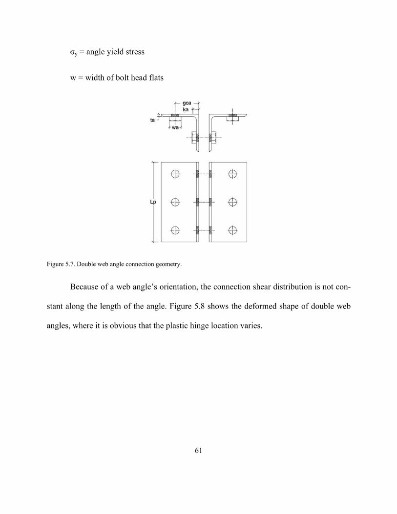
Figure 5.8. Deformed double web angle connection. ....................................................................62
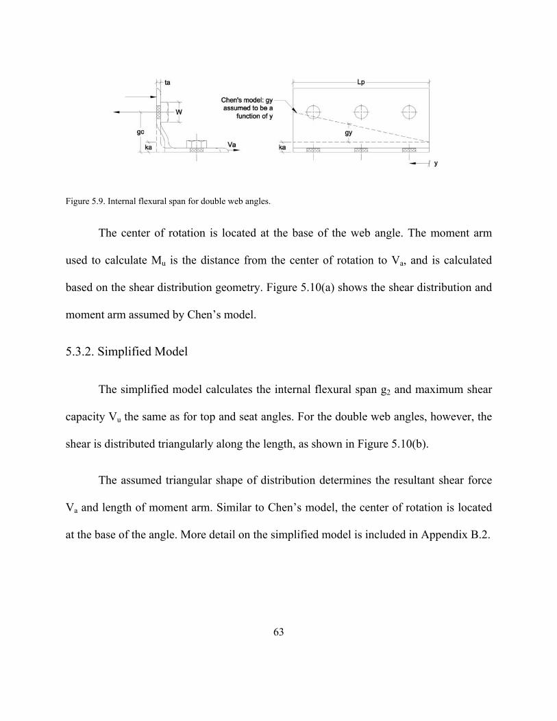
Figure 5.9. Internal flexural span for double web angles. .............................................................63
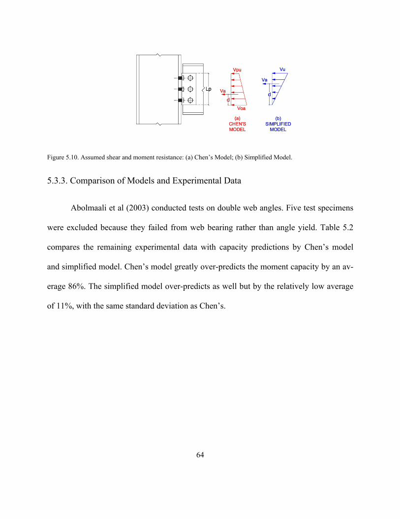
Figure 5.10. Assumed shear and moment resistance: (a) Chen’s Model; (b) Simplified Model. ..64
Figure 5.11. Top and seat angles with double web angles connection geometry. .........................67
Figure 5.12. Shear distribution in web angles for Type 2 connections (simplified model). ..........69
Figure A.1. Maximum shear resistance in angle leg assuming double bending. ...........................91
Figure A.2. Moment arm of maximum shear resistance of top and seat angle connection
(simplified model). .........................................................................................................................92
Figure B.1. Deformed double web angle connection. ...................................................................97
Figure B.2. Approximation of g2: (a) Top and seat angles; (b) Web angles ..................................98
Figure B.3. Assumed shear resistance of double web angles (Chen’s Model) ..............................99
Figure B.4. Assumed shear resistance of double web angles (Simplified model) .......................103
Figure C.1. Shear distribution in web angles for Type 2 connections (simplified model). .........114
9
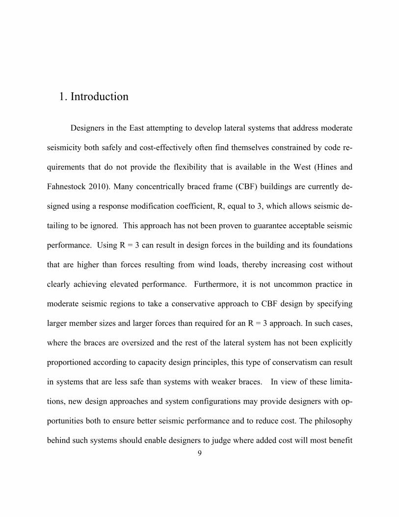
1. Introduction
Designers in the East attempting to develop lateral systems that address moderate
seismicity both safely and cost-effectively often find themselves constrained by code re-
quirements that do not provide the flexibility that is available in the West (Hines and
Fahnestock 2010). Many concentrically braced frame (CBF) buildings are currently de-
signed using a response modification coefficient, R, equal to 3, which allows seismic de-
tailing to be ignored. This approach has not been proven to guarantee acceptable seismic
performance. Using R = 3 can result in design forces in the building and its foundations
that are higher than forces resulting from wind loads, thereby increasing cost without
clearly achieving elevated performance. Furthermore, it is not uncommon practice in
moderate seismic regions to take a conservative approach to CBF design by specifying
larger member sizes and larger forces than required for an R = 3 approach. In such cases,
where the braces are oversized and the rest of the lateral system has not been explicitly
proportioned according to capacity design principles, this type of conservatism can result
in systems that are less safe than systems with weaker braces. In view of these limita-
tions, new design approaches and system configurations may provide designers with op-
portunities both to ensure better seismic performance and to reduce cost. The philosophy
behind such systems should enable designers to judge where added cost will most benefit
10
system performance.
Empirical evidence indicates that steel braced frames possess appreciable reserve
capacity – in the form of gravity framing and gusset plate connections. These partially-
restrained connection elements form a “reserve” moment frame system that can prevent
sidesway collapse even when the primary lateral force resisting system (LFRS) is signifi-
cantly damaged due to brace fracture. When required, reserve capacity can be enhanced
without significant expense. As summarized by Hines et al. (2009), collapse perfor-
mance of CBF systems that possess limited ductility appears to be impacted less by a sys-
tem’s strength than by its reserve capacity. It is therefore proposed to reconsider the de-
sign of braced frames in low and moderate seismic regions as moderate-ductility dual
systems. Such dual system behavior can be viewed from two different perspectives:
1. A stiff primary braced frame with a moment frame reserve system to prevent
collapse in the event of brace failure.
2. A flexible moment frame stiffened by a sacrificial braced frame designed to
withstand wind loads and to provide service-level drift control.
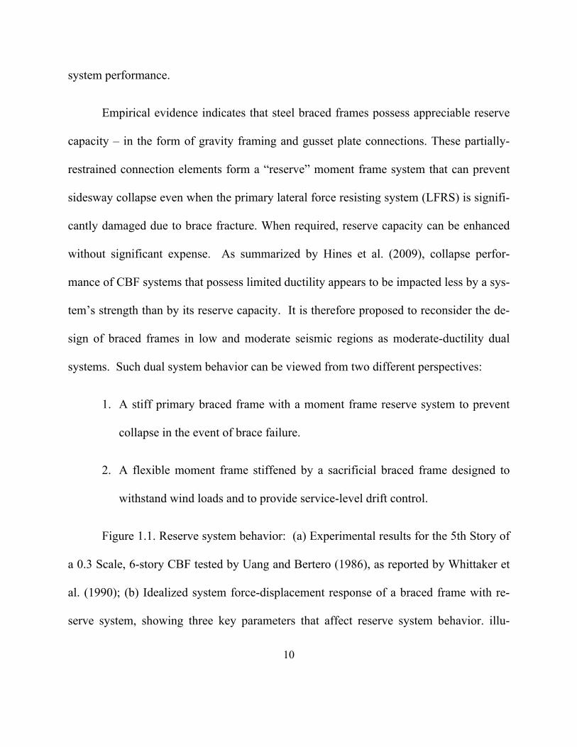
Figure 1.1. Reserve system behavior: (a) Experimental results for the 5th Story of
a 0.3 Scale, 6-story CBF tested by Uang and Bertero (1986), as reported by Whittaker et
al. (1990); (b) Idealized system force-displacement response of a braced frame with re-
serve system, showing three key parameters that affect reserve system behavior. illu-
11
strates the idea behind moderate-ductility dual systems. In contrast to high seismic de-
sign, where system ductility is achieved through large component ductility, e.g., plastic
hinges, brace buckling or brace yielding, moderate-ductility dual systems achieve system
ductility through the coupling of a stiff system with a flexible system. The stiff CBF sys-
tem is expected to perform in a brittle manner; however, if the flexible system possesses
sufficient strength, stiffness and ductility to prevent collapse, then adequate system duc-
tility has been achieved.
Figure 1.1. Reserve system behavior: (a) Experimental results for the 5th Story of a 0.3 Scale, 6-story CBF tested by Uang and Bertero (1986), as reported by Whittaker et al. (1990); (b) Idealized system force-displacement re-sponse of a braced frame with reserve system, showing three key parameters that affect reserve system behavior.
The strength, elastic stiffness and ductility of the reserve system are represented
by the numbers 1, 2 and 3 in Figure 1.1(b). It is possible to imagine a successful reserve
system that has very little ductility (3) of its own. In this instance, system ductility would
be achieved without relying on any component ductility. Figure 1.1(a) shows the per-
formance of the 5th story of a 6-story, 0.3 scale, CBF dual system tested at the University
of California, Berkeley in the mid 1980s. To this authors’ knowledge, these are the only
12
published test results demonstrating the experimental performance of reserve system ca-
pacity based on a large-scale shake table test. Figure 1.1 (a) differs significantly from
Figure 1.1 (b) in that the reserve system is nearly as stiff, and significantly stronger than
the primary CBF. Since the testing at Berkeley was part of a larger joint research venture
between the U.S. and Japan in the 1980s, this design resulted from design criteria assem-
bled to satisfy both U.S. and Japanese building codes that were then current. Considering
the strength, stiffness and ductility of reserve systems as shown in Figure 1.1 (b) as fun-
damental to collapse performance of low-ductility steel CBFs, it becomes clear that the
significant stiffness and strength discontinuities in such systems present challenges for
the proper analysis of these systems. Furthermore, considering that collapse is the per-
formance level in question for such systems, the ability of such analyses to predict col-
lapse becomes of paramount importance. The interconnected nature of this problem,
which includes low-ductility system performance, appropriate ground motion suite selec-
tion and careful consideration probabilistic methods for collapse risk assessment has been
discussed at length by Hines et al. (2009, 2010, 2011). Ongoing large-scale component
testing by Stoakes and Fahnestock (2010, 2011) has demonstrated that reserve capacity
may be designed into standard braced frame gusset plate connections for relatively little
cost, and work is underway to assemble the resources necessary for shake table testing of
low-ductility CBFs with reserve systems at large-scale or full-scale.This report discusses
the results of analytical work conducted since the printing of Hines et al’s 2009 paper.
Recognizing the problematic nature not only of assessing the non-linear dynamic beha-

13
vior of these systems but also of making these assessments up to the point of system col-
lapse, the authors have attempted to re-frame the question of reserve system behavior on
a fundamental level. Models have been simplified in order to isolate the key strength and
stiffness discontinuities between the primary CBF and the reserve system. These simple
models have been constructed in two different software packages, Ruaumoko (Carr 2004)
and OpenSees (2007) in an attempt to distinguish issues related to physical collapse from
issues related to numerical convergence.
After discussing the challenges of modeling braced frames with reserve systems,
this report introduces a discussion on partially restrained moment connections that could
be used with existing gravity framing to create reliable and efficient reserve systems. A
preferred connection for “Type II construction” (Disque 1976, Geschwinder and Disque
2005) PR-connections that consist of bolted top and seat angles with bolted double web
angles have the ability to provide significant moment-rotation capacity in gravity framing
connections for very little added cost. These connections and their use in Type II con-
struction have a long and interesting history that has focused primarily on their use for
resisting wind loads in the elastic range. This report and this research approaches these
connections with a primary interest in their ultimate moment and rotation capacity and its
potential to enhance gravity system lateral reserve capacity economically.
14
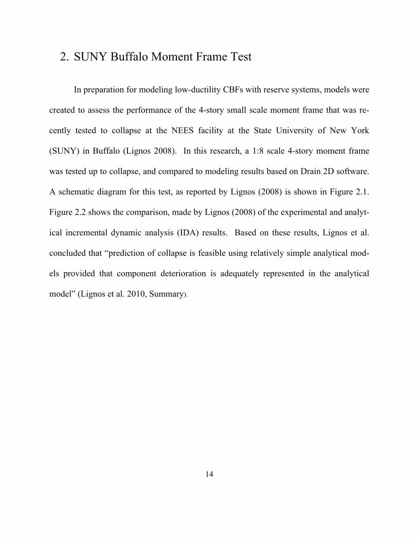
2. SUNY Buffalo Moment Frame Test
In preparation for modeling low-ductility CBFs with reserve systems, models were
created to assess the performance of the 4-story small scale moment frame that was re-
cently tested to collapse at the NEES facility at the State University of New York
(SUNY) in Buffalo (Lignos 2008). In this research, a 1:8 scale 4-story moment frame
was tested up to collapse, and compared to modeling results based on Drain 2D software.
A schematic diagram for this test, as reported by Lignos (2008) is shown in Figure 2.1.
Figure 2.2 shows the comparison, made by Lignos (2008) of the experimental and analyt-
ical incremental dynamic analysis (IDA) results. Based on these results, Lignos et al.
concluded that “prediction of collapse is feasible using relatively simple analytical mod-
els provided that component deterioration is adequately represented in the analytical
model” (Lignos et al. 2010, Summary).

15
Figure 2.1. Schematic of 4-story moment frame prototype on which 1:8 scale test frame was based.
Figure 2.2: Buffalo Frame IDA Comparison (Lignos 2008, Figure 7.26).
Rotational springs were used to model the hinge areas of beams and columns. The
P-Delta load was applied to the leaning column which was modeled as an elastic beam
column element and connected to the frame using truss elements. The P- geometric
transformation was used to include the large displacement in the model. In the Ruaumoko
16
model, a bilinear inelastic hysteresis rule was used to model nonlinear behavior of the
beams, assuming ILOS=0 implying no strength degradation. This model also has an elas-
tic beam column element with large area to model the leaning column which is connected
to the frame by a rigid link.
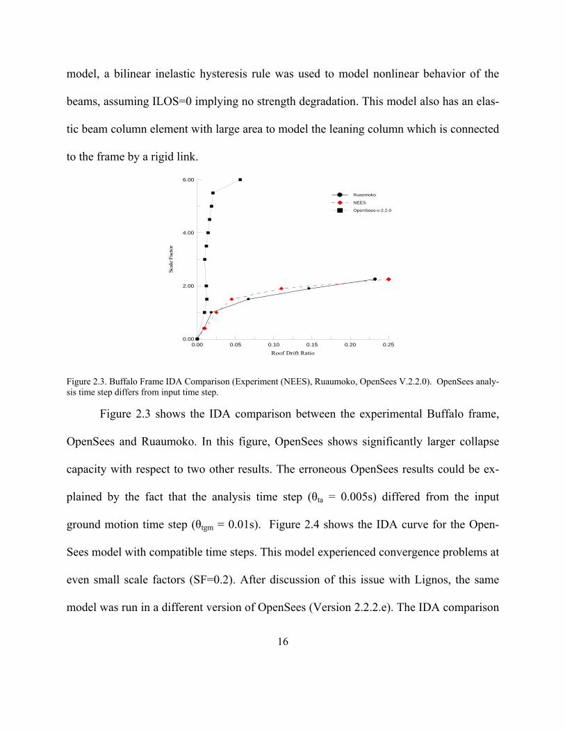
Figure 2.3. Buffalo Frame IDA Comparison (Experiment (NEES), Ruaumoko, OpenSees V.2.2.0). OpenSees analy-sis time step differs from input time step.
Figure 2.3 shows the IDA comparison between the experimental Buffalo frame,
OpenSees and Ruaumoko. In this figure, OpenSees shows significantly larger collapse
capacity with respect to two other results. The erroneous OpenSees results could be ex-
plained by the fact that the analysis time step (θta = 0.005s) differed from the input
ground motion time step (θtgm = 0.01s). Figure 2.4 shows the IDA curve for the Open-
Sees model with compatible time steps. This model experienced convergence problems at
even small scale factors (SF=0.2). After discussion of this issue with Lignos, the same
model was run in a different version of OpenSees (Version 2.2.2.e). The IDA comparison
0.00 0.05 0.10 0.15 0.20 0.25
Roof Drift Ratio
0.00
2.00
4.00
6.00
Sca
le F
acto
r
Ruaomoko
NEES
OpenSees-v-2.2.0

17
between OpenSees V.2.2.2.e, Ruaumoko and experimental data is showed in Figure 2.5.
It can be seen that the IDA curves have significantly better correlation.
Figure 2.4. Buffalo Frame IDA Comparison (NEES, Ruaumoko, OpenSees V.2.2.0). OpenSees analysis time step is the same as the ground motion input time step.
Figure 2.5. Buffalo Frame IDA Comparison (Experiment (NEES), Ruaumoko, OpenSees V.2.2.2.e). OpenSees analysis time step is the same as the ground motion input time step
0.00 0.05 0.10 0.15 0.20 0.25
Roof Drift Ratio
0.00
2.00
4.00
6.00
Sca
le F
acto
r
Ruaomoko
NEES
OpenSees-V.2.2.O
0.00 0.05 0.10 0.15 0.20 0.25
Roof Drift Ratio
0.00
2.00
4.00
6.00
Sca
le F
acto
r
Ruaomoko
NEES
OpenSees-v.2.2.e
18
3. One-Story System Analysis
3.1 Scope
In an effort to establish benchmarks for the comparison of Ruaumoko and Open-
Sees, a series of 1-story models were created. These models are:
-Single Cantilever
-Moment Resisting Frame (MRF)
-Eccentrically Braced Frame (EBF)
-Low-Ductility Concentrically Braced Frame (CBF)
While this research is concerned primarily with the performance of Low-Ductility
CBFs, the difficulties in modeling such frames up to collapse led to the decision to estab-
lish baseline models of more ductile systems. Results from these models (presented in
Sections 3.3 through 3.5) demonstrate a high degree of consistency between Ruaumoko
and OpenSees for dynamic analysis of materially and geometrically non-linear systems.
When compared to results for the low-ductility CBF in Section 3.6, the consistency in
these more traditional, ductile systems helps to emphasize the uniqueness of low-ductility
CBFs with reserve systems in terms of collapse performance and modeling. The large
discontinuities in stiffness and strength experienced by these systems pose modeling
challenges that simply are not present in more traditional systems.
19
3.2. Ground Motions
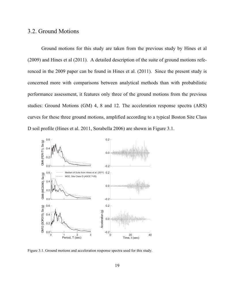
Ground motions for this study are taken from the previous study by Hines et al
(2009) and Hines et al (2011). A detailed description of the suite of ground motions refe-
renced in the 2009 paper can be found in Hines et al. (2011). Since the present study is
concerned more with comparisons between analytical methods than with probabilistic
performance assessment, it features only three of the ground motions from the previous
studies: Ground Motions (GM) 4, 8 and 12. The acceleration response spectra (ARS)
curves for these three ground motions, amplified according to a typical Boston Site Class
D soil profile (Hines et al. 2011, Sorabella 2006) are shown in Figure 3.1.
Figure 3.1. Ground motions and acceleration response spectra used for this study.
0 1 2 3Period, T (sec)
0.0
0.2
0.4
0.6
GM
8(M
CD
090),
Sa
(g) Median of Suite from Hines et al. (2011)
MCE, Site Class D (ASCE 7-05)
0.0
0.2
0.4
0.6
GM
12
(SO
R315),
Sa
(g)
0.0
0.2
0.4
0.6
GM
4(F
ER
-T1),
Sa
(g)
0 20 40Time, t (sec)
-0.2
0.0
0.2
Acc
ele
ratio
n(g
)
-0.2
0.0
0.2
-0.2
0.0
0.2
20
3.3 Cantilever
3.3.1. Model Setup
The first system is a simple cantilever which forms a plastic hinge at the
base, shown in Figure 3.2. This cantilever represents the reserve system of other simple
models which is equivalent to the moment frame of the first story of the nine story model
( for ¼ of the building, see chapter 4). To find the equivalent section a push over analysis
was done on the first story of the nine story model and non-linear force-displacement re-
sponse of the cantilever including P-∆ effects was calibrated to approximate the pushover
curve for the first story of the 9-story building reserve system. Instead of adding a
second leaning column to assume the remainder of the building weight, the area of the
leaning column was increased to maintain axial stresses similar to the first floor graving
framing columns. The resulting section is approximately 10.2 in. deep and 46 in. wide.
The column vertical load is approximately equal to ¼ of the nine story building. The col-
umn material is steel, with E = 29,000 ksi, Fy = 46 ksi, and a linear strain hardening
modulus of Esh = 290 ksi. Note that these numbers were chosen to approximate the force
displacement behavior of the first story reserve system, not to model an actual steel col-
umn. For this reason, it is not necessary for the cantilevered column in Figure 3.2 to be
considered realistic in its own right. Figure 3.3 compares the pushover curves for the re-
serve system in Figure 3.2 and the first story reserve system for ¼ of the 9-story building.
For the assessment of the first story reserve system, the second story was also modeled

21
with braces intact so as to allow the gravity columns to contribute to the reserve capacity
in addition to the gravity beams. In Ruaumoko, the plastic hinge length was set at half of
the column depth or 5.1 in. In OpenSees, the column has 4 fibers along the depth and 16
fibers along the width.
Figure 3.2. Cantilever system
Figure 3.3. Comparison of reserve system pushover curves between SDOF in Figure 4 and the first floor reserve system for ¼ of the 9-story building
0.00 0.02 0.04 0.06 0.08 0.10
Drift(%)
-150
-100
-50
0
50
100
For
ce (k)
1/9 Story
Cantilever
22
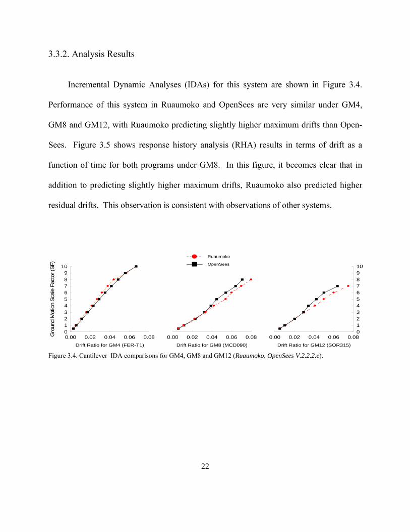
3.3.2. Analysis Results
Incremental Dynamic Analyses (IDAs) for this system are shown in Figure 3.4.
Performance of this system in Ruaumoko and OpenSees are very similar under GM4,
GM8 and GM12, with Ruaumoko predicting slightly higher maximum drifts than Open-
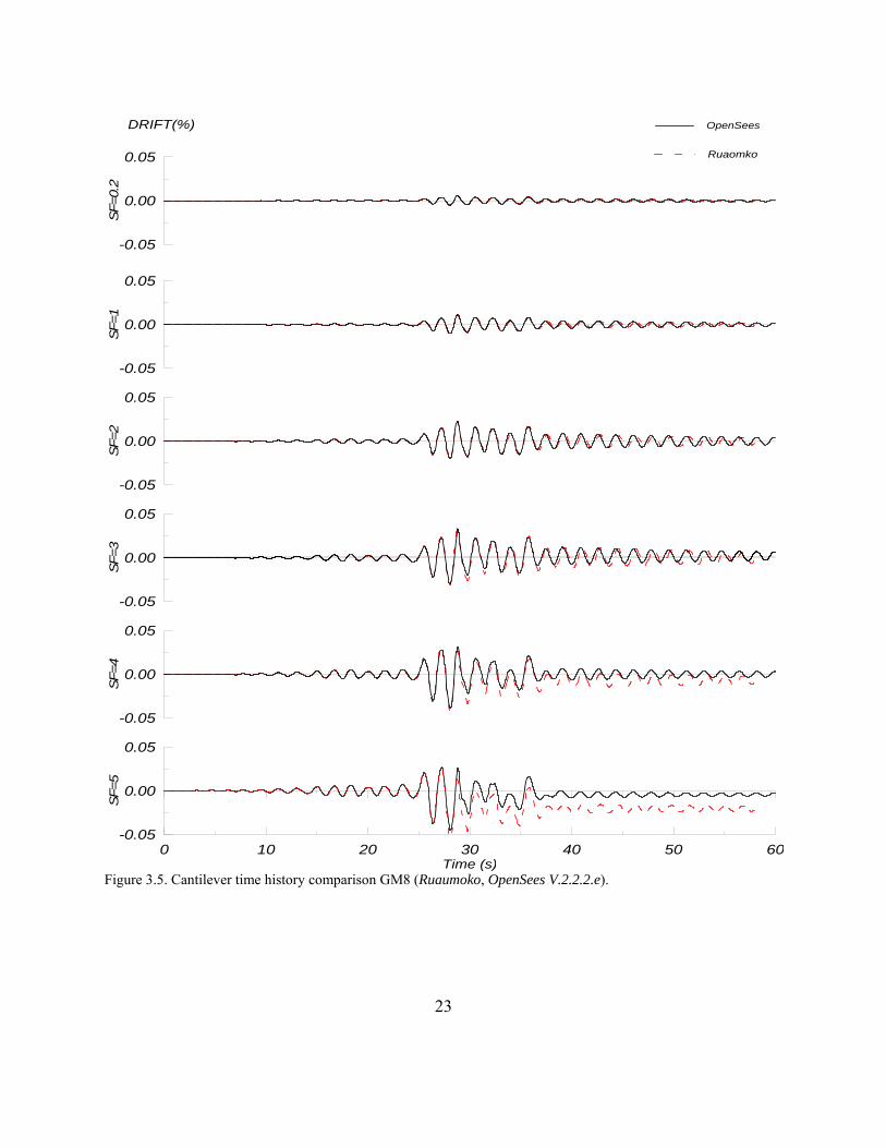
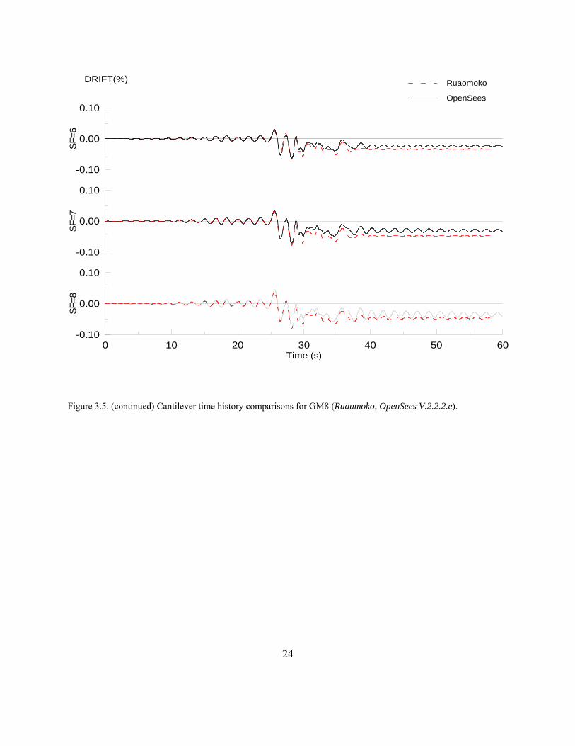
Sees. Figure 3.5 shows response history analysis (RHA) results in terms of drift as a
function of time for both programs under GM8. In this figure, it becomes clear that in
addition to predicting slightly higher maximum drifts, Ruaumoko also predicted higher
residual drifts. This observation is consistent with observations of other systems.
Figure 3.4. Cantilever IDA comparisons for GM4, GM8 and GM12 (Ruaumoko, OpenSees V.2.2.2.e).
0.00 0.02 0.04 0.06 0.08
Drift Ratio for GM4 (FER-T1)
0123456789
10
Gro
und
Mot
ion
Sca
le F
acto
r (S
F)
Ruaumoko
OpenSees
0.00 0.02 0.04 0.06 0.08
Drift Ratio for GM8 (MCD090)
0.00 0.02 0.04 0.06 0.08
Drift Ratio for GM12 (SOR315)
012345678910
23
Figure 3.5. Cantilever time history comparison GM8 (Ruaumoko, OpenSees V.2.2.2.e).
0 10 20 30 40 50 60Time (s)
-0.05
0.00
0.05
SF=0.
2OpenSees
Ruaomko
-0.05
0.00
0.05
SF=1
-0.05
0.00
0.05
SF=2
-0.05
0.00
0.05
SF=3
-0.05
0.00
0.05
SF=4
-0.05
0.00
0.05
SF=5
DRIFT(%)
24
Figure 3.5. (continued) Cantilever time history comparisons for GM8 (Ruaumoko, OpenSees V.2.2.2.e).
0 10 20 30 40 50 60Time (s)
-0.10
0.00
0.10
SF=6
-0.10
0.00
0.10
SF=7
-0.10
0.00
0.10
SF
=8
DRIFT(%) Ruaomoko
OpenSees

25
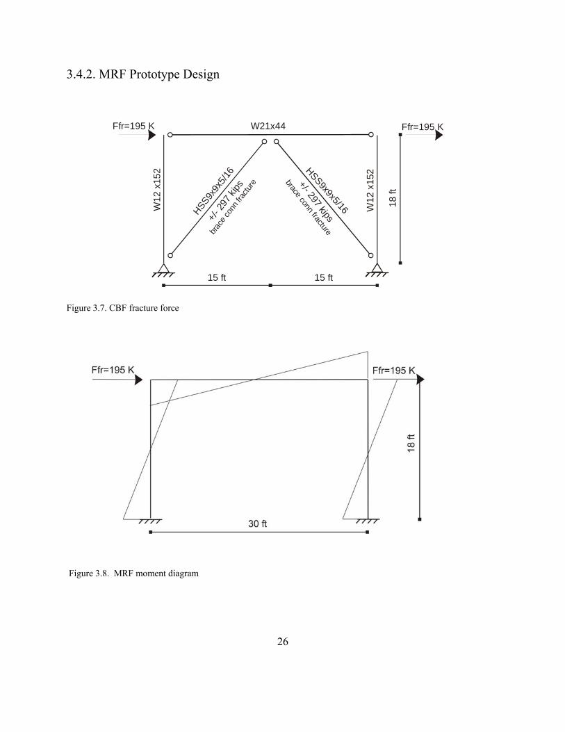
3.4 Moment Resisting Frame
3.4.1. Model Setup
The next simple model which is shown in Figure 3.6 is considered to be a
moment frame connected to a cantilever as a reserve system. The reserve system is the
same as the cantilever column of Section 3.3. As it will be discussed more in the section
3.6 the braces in the 9-story model are assumed to fracture at a force of 297 kips at their
connections prior to buckling. The moment frame is designed to resistant a lateral load
equivalent to this fracture force. The material and hinge properties in OpenSees and
Ruaumoko are the same as the cantilever model. The P-∆ geometric transformation was
used to include the large displacement in the model.
Figure 3.6. Moment Resisting Frame system.
26
3.4.2. MRF Prototype Design
Figure 3.7. CBF fracture force
Figure 3.8. MRF moment diagram
18
ft
W1
2 x
152
W1
2 x
152
Ffr=195 K
HSS9x
9x5/
16
HSS9x9x5/16
15 ft15 ft
+/- 2
97 k
ips
brac
e co
nn fr
actu
re +/- 297 kips
brace conn fracture
W21x44 Ffr=195 K

27
:
21060 458 24 162
:
1.1 1.1 468 566 14 311
21060
450
14 311:
91.4 4330 4.2
18 124.2
51.4 107
0.658 38.58
38.58 91.4 3526
1.2 4500.9 3526
89
21060
0.9 603 46 1 1.2 450107 91.4
0.963
28
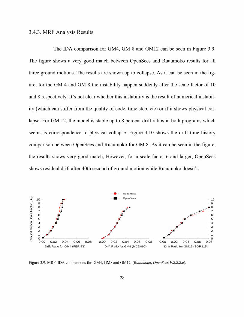
3.4.3. MRF Analysis Results
The IDA comparison for GM4, GM 8 and GM12 can be seen in Figure 3.9.
The figure shows a very good match between OpenSees and Ruaumoko results for all
three ground motions. The results are shown up to collapse. As it can be seen in the fig-
ure, for the GM 4 and GM 8 the instability happen suddenly after the scale factor of 10
and 8 respectively. It’s not clear whether this instability is the result of numerical instabil-
ity (which can suffer from the quality of code, time step, etc) or if it shows physical col-
lapse. For GM 12, the model is stable up to 8 percent drift ratios in both programs which
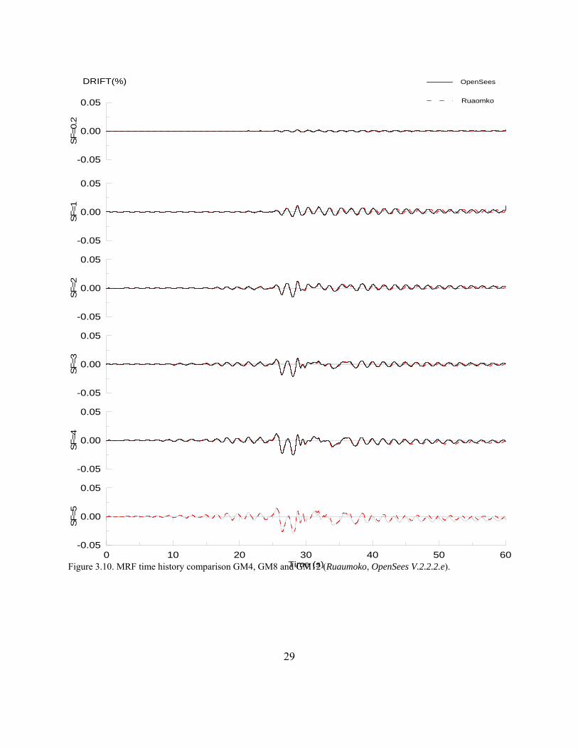
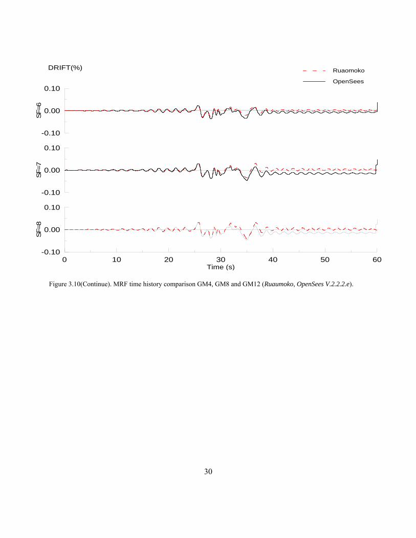
seems is correspondence to physical collapse. Figure 3.10 shows the drift time history
comparison between OpenSees and Ruaumoko for GM 8. As it can be seen in the figure,
the results shows very good match, However, for a scale factor 6 and larger, OpenSees
shows residual drift after 40th second of ground motion while Ruaumoko doesn’t.
Figure 3.9. MRF IDA comparisons for GM4, GM8 and GM12 (Ruaumoko, OpenSees V.2.2.2.e).
0.00 0.02 0.04 0.06 0.08
Drift Ratio for GM4 (FER-T1)
0123456789
10
Gro
und
Mot
ion
Sca
le F
acto
r (S
F)
Ruaumoko
OpenSees
0.00 0.02 0.04 0.06 0.08
Drift Ratio for GM8 (MCD090)
0.00 0.02 0.04 0.06 0.08
Drift Ratio for GM12 (SOR315)
012345678910
29
Figure 3.10. MRF time history comparison GM4, GM8 and GM12 (Ruaumoko, OpenSees V.2.2.2.e).
0 10 20 30 40 50 60Time (s)
-0.05
0.00
0.05
SF=0.
2OpenSees
Ruaomko
-0.05
0.00
0.05
SF=1
-0.05
0.00
0.05
SF=2
-0.05
0.00
0.05
SF=3
-0.05
0.00
0.05
SF=4
-0.05
0.00
0.05
SF=5
DRIFT(%)
30
Figure 3.10(Continue). MRF time history comparison GM4, GM8 and GM12 (Ruaumoko, OpenSees V.2.2.2.e).
0 10 20 30 40 50 60Time (s)
-0.10
0.00
0.10
SF=6
-0.10
0.00
0.10
SF=7
-0.10
0.00
0.10
SF=8
DRIFT(%) Ruaomoko
OpenSees
31
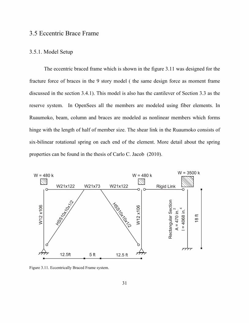
3.5 Eccentric Brace Frame
3.5.1. Model Setup
The eccentric braced frame which is shown in the figure 3.11 was designed for the
fracture force of braces in the 9 story model ( the same design force as moment frame
discussed in the section 3.4.1). This model is also has the cantilever of Section 3.3 as the
reserve system. In OpenSees all the members are modeled using fiber elements. In
Ruaumoko, beam, column and braces are modeled as nonlinear members which forms
hinge with the length of half of member size. The shear link in the Ruaumoko consists of
six-bilinear rotational spring on each end of the element. More detail about the spring
properties can be found in the thesis of Carlo C. Jacob (2010).
Figure 3.11. Eccentrically Braced Frame system.
32
3.5.2. Prototype Design
Figure 3.12. EBF moment diagram
33
:
1.1 1.25 172 46 11132
11132 260
371
3713
1292.7
371 92.7 . 556 10 10 1/2
:
371
470
1.2 470 371 935 12 106
:
0.9
111320.9 46
269 21 122
34
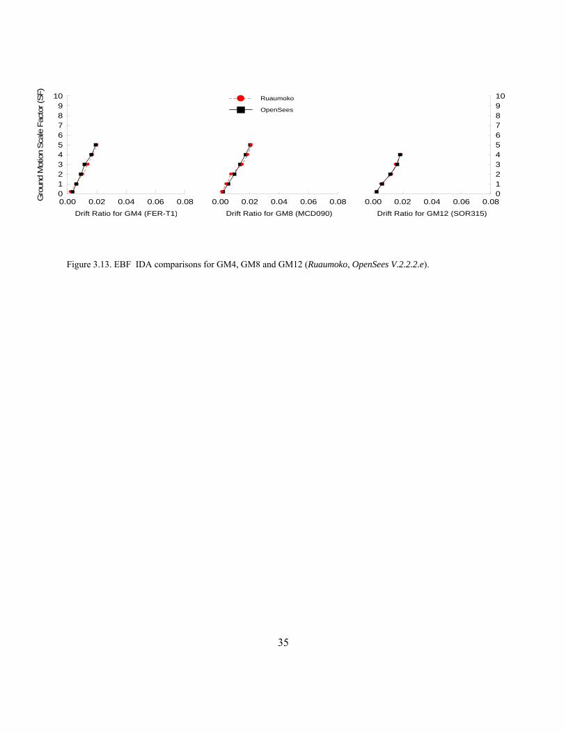
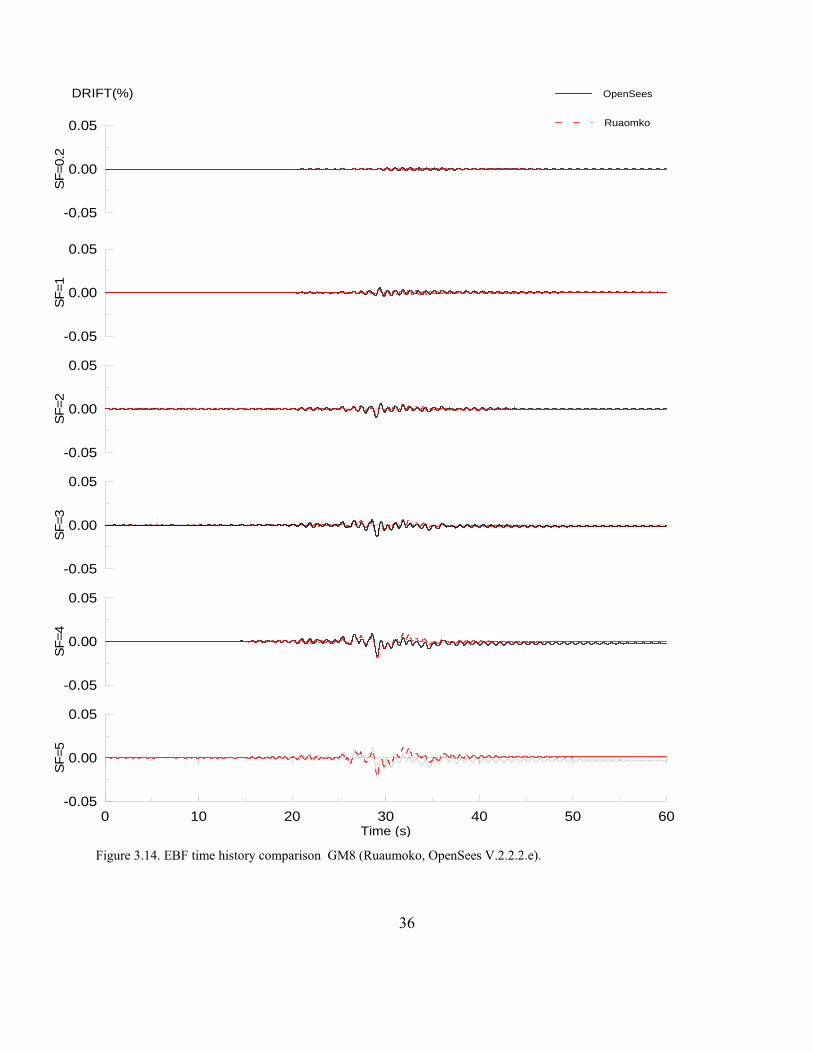
3.5.3. EBF Analysis Results
Figure 3.13 shows the IDA comparison between OpenSees and Ruaumoko for the
mentioned EBF model for GM4, GM8 and GM12 . As it can be seen in the figure there is
a very good match between these two software results. The results for each ground mo-
tions are shown up to the scale factor which is associated with collapse. In this model, the
shear link rotation of about 8 percent is considered as the collapse level. The drift time
history comparison between OpenSees and Ruaumoko can be seen in the Figure 3.14.
This figure indicates that the drift time history response of two models match well to-
gether. The only considerable difference between results is the residual displacements. As
it can be seen in the figure after 40th second OpenSees shows some residual displacement
while Ruaumoko doesn’t. A it discussed before, this difference in free vibration zone ex-
ists in all other models. It’s interesting to note that sometimes OpenSees shows this resi-
dual displacement and sometimes Ruaumoko does. Currently the reason of this difference
is not obvious for the authors. In EBF this difference also can be seen in the vertical dis-
placement of shear link end nodes which cause some differences in the shear – rotation
hysteresis loop of the shear link.
35
Figure 3.13. EBF IDA comparisons for GM4, GM8 and GM12 (Ruaumoko, OpenSees V.2.2.2.e).
0.00 0.02 0.04 0.06 0.08
Drift Ratio for GM4 (FER-T1)
0123456789
10
Gro
und
Mot
ion
Sca
le F
acto
r (S
F)
Ruaumoko
OpenSees
0.00 0.02 0.04 0.06 0.08
Drift Ratio for GM8 (MCD090)
0.00 0.02 0.04 0.06 0.08
Drift Ratio for GM12 (SOR315)
012345678910
36
Figure 3.14. EBF time history comparison GM8 (Ruaumoko, OpenSees V.2.2.2.e).
0 10 20 30 40 50 60Time (s)
-0.05
0.00
0.05
SF
=0.
2
OpenSees
Ruaomko
-0.05
0.00
0.05
SF
=1
-0.05
0.00
0.05
SF
=2
-0.05
0.00
0.05
SF=3
-0.05
0.00
0.05
SF
=4
-0.05
0.00
0.05
SF
=5
DRIFT(%)
37
3.6 Low-Ductility CBF
3.6.1. Model Setup
Based on the IDA and displacement time history comparison between OpenSees
and Ruaumoko for ductile systems (section 3.3 through 3.5), the nonlinear behavior of
these systems can be modeled with high confidence. Figure 3.15 shows the simplified
model of the concentrically braced frame created to facilitate comparisons of non-ductile
systems between OpenSees and Ruaumoko. The braced frame is similar to the braced
frame on the first story of the 9-story building shown in Figure 4.1. Braces are assumed
to fracture at a force of 297 kips at their connections prior to buckling. Both braces are
modeled to fracture at the same time. This violates the idea that if the braces assume load
from the floor above, the compression brace will fracture first, however it simplifies the
behavior of the model and allows for more direct study of reserve capacity at a concep-
tual level. Brace fracture is modeled in Ruaumoko as described in Hines et al. (2009).
Brace fracture is modeled in OpenSees by removing the brace from the model (death of
the element) after it is subjected to the fracture force.
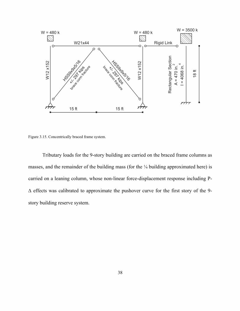
38
Figure 3.15. Concentrically braced frame system.
Tributary loads for the 9-story building are carried on the braced frame columns as
masses, and the remainder of the building mass (for the ¼ building approximated here) is
carried on a leaning column, whose non-linear force-displacement response including P-
effects was calibrated to approximate the pushover curve for the first story of the 9-
story building reserve system.
W = 3500 k
18
ft
Rigid LinkW
12
x152
W12
x152
W21x44
HSS9x
9x5/
16
HSS9x9x5/16
15 ft15 ft
+/-29
7ki
ps
brac
eco
nnfrac
ture +/-
297kips
braceconn
fracture
Recta
ngula
rS
ection
A=
470
in.
I=
4068
in.2 4
W = 480 kW = 480 k
39
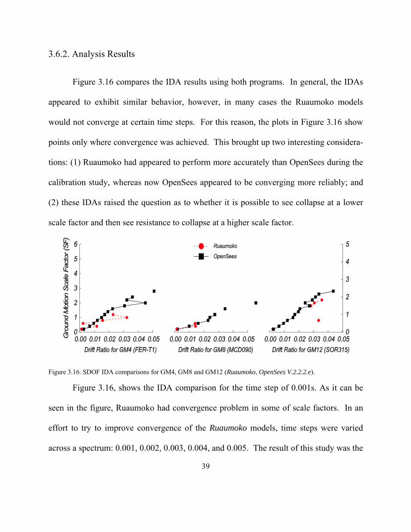
3.6.2. Analysis Results
Figure 3.16 compares the IDA results using both programs. In general, the IDAs
appeared to exhibit similar behavior, however, in many cases the Ruaumoko models
would not converge at certain time steps. For this reason, the plots in Figure 3.16 show
points only where convergence was achieved. This brought up two interesting considera-
tions: (1) Ruaumoko had appeared to perform more accurately than OpenSees during the
calibration study, whereas now OpenSees appeared to be converging more reliably; and
(2) these IDAs raised the question as to whether it is possible to see collapse at a lower
scale factor and then see resistance to collapse at a higher scale factor.
Figure 3.16. SDOF IDA comparisons for GM4, GM8 and GM12 (Ruaumoko, OpenSees V.2.2.2.e).
Figure 3.16, shows the IDA comparison for the time step of 0.001s. As it can be
seen in the figure, Ruaumoko had convergence problem in some of scale factors. In an
effort to try to improve convergence of the Ruaumoko models, time steps were varied
across a spectrum: 0.001, 0.002, 0.003, 0.004, and 0.005. The result of this study was the
40
observation that under different ground motions, the Ruaumoko models converged better
or worse under different time steps. Smaller time steps did not always yield more consis-
tent results. This led to the intensive calculation of IDA curves assuming every one of
the five time steps listed above. The IDAs plotted in Figures 3.18 through 3.20 reflect
the selection of the most consistent IDA from the different time step runs.
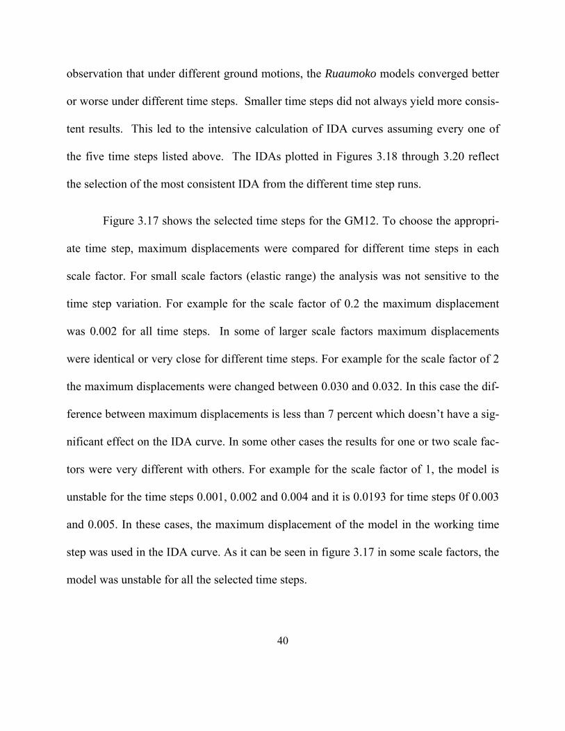
Figure 3.17 shows the selected time steps for the GM12. To choose the appropri-
ate time step, maximum displacements were compared for different time steps in each
scale factor. For small scale factors (elastic range) the analysis was not sensitive to the
time step variation. For example for the scale factor of 0.2 the maximum displacement
was 0.002 for all time steps. In some of larger scale factors maximum displacements
were identical or very close for different time steps. For example for the scale factor of 2
the maximum displacements were changed between 0.030 and 0.032. In this case the dif-
ference between maximum displacements is less than 7 percent which doesn’t have a sig-
nificant effect on the IDA curve. In some other cases the results for one or two scale fac-
tors were very different with others. For example for the scale factor of 1, the model is
unstable for the time steps 0.001, 0.002 and 0.004 and it is 0.0193 for time steps 0f 0.003
and 0.005. In these cases, the maximum displacement of the model in the working time
step was used in the IDA curve. As it can be seen in figure 3.17 in some scale factors, the
model was unstable for all the selected time steps.

41
Figure 3.17. Selected analysis time step for Ruaumoko model for GM12.
Figure 3.18 shows dramatic improvement in the convergence of the Ruaumoko
models based on the selection of appropriate time steps Currently, it is not clear why var-
iation of the time step—sometimes as an increase, sometimes as a decrease, ensures bet-
ter convergence of the Ruaumoko models. It is also not clear why the OpenSees models
appear to be more stable in the context of this SDOF reserve system when they appeared
to perform worse than the Ruaumoko models during the calibration study with the Buffa-
lo frame. Figure 3.18 still shows some non-convergence at lower scale factors and then
resumed convergence at higher scale factors. Currently, it also remains unknown wheth-
er this non-convergence is numerical or whether it represents physical collapse.
0.00 0.01 0.02 0.03 0.04 0.05
Drift Ratio for GM12 (SOR315)
0.00
0.50
1.00
1.50
2.00
2.50
3.00
3.50
4.00
4.50
5.00
Gro
und
Motio
nS
cale
Fact
or(
SF)
Ruaomoko
All
All
All
All
0.004,5
All
0.005
0.003,5
0.002,3,4,5
0.002,4,5
0.003
42
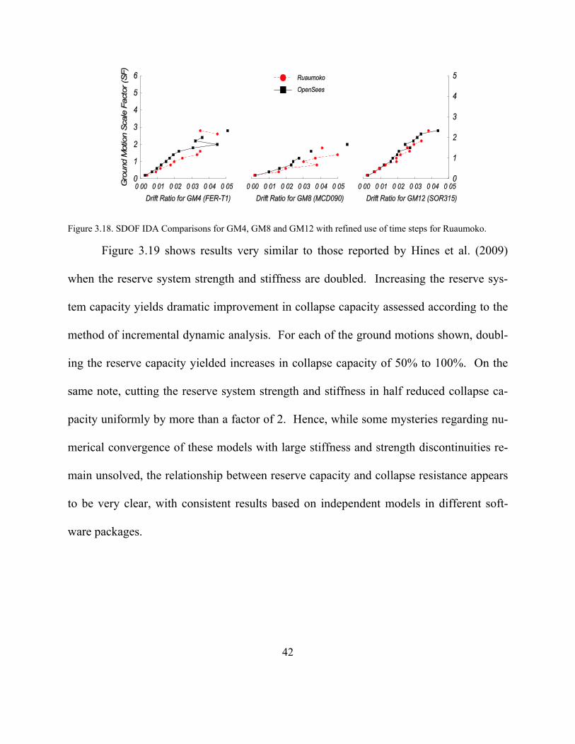
Figure 3.18. SDOF IDA Comparisons for GM4, GM8 and GM12 with refined use of time steps for Ruaumoko.
Figure 3.19 shows results very similar to those reported by Hines et al. (2009)
when the reserve system strength and stiffness are doubled. Increasing the reserve sys-
tem capacity yields dramatic improvement in collapse capacity assessed according to the
method of incremental dynamic analysis. For each of the ground motions shown, doubl-
ing the reserve capacity yielded increases in collapse capacity of 50% to 100%. On the
same note, cutting the reserve system strength and stiffness in half reduced collapse ca-
pacity uniformly by more than a factor of 2. Hence, while some mysteries regarding nu-
merical convergence of these models with large stiffness and strength discontinuities re-
main unsolved, the relationship between reserve capacity and collapse resistance appears
to be very clear, with consistent results based on independent models in different soft-
ware packages.
43
Figure 3.19. CBF IDA Comparisons for GM4, GM8 and GM12 with refined use of time steps for Ruaumoko. Re-serve system strengths and stiffnesses are doubled in comparison with the IDAs shown in Figure 3.18.
Figure 3.20. CBF IDA Comparisons for GM4, GM8 and GM12 with refined use of time steps for Ruaumoko. Re-serve system strengths and stiffnesses are halved in comparison with the IDAs shown in Figure 3.18.
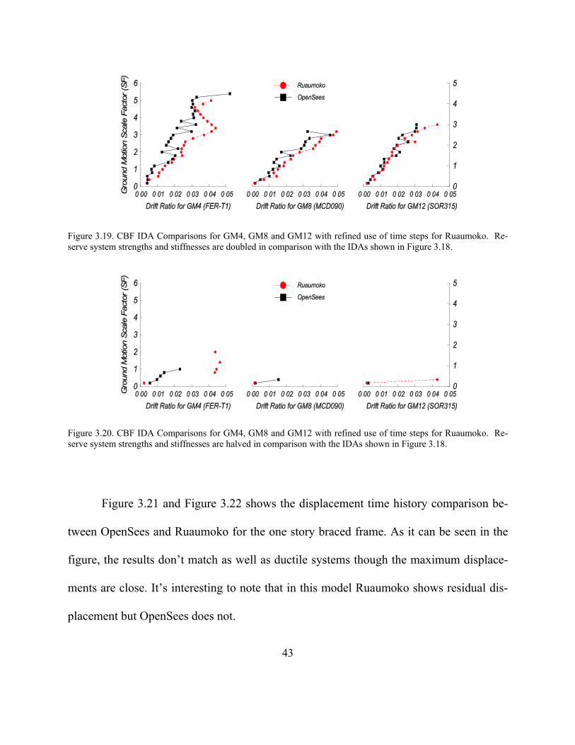
Figure 3.21 and Figure 3.22 shows the displacement time history comparison be-
tween OpenSees and Ruaumoko for the one story braced frame. As it can be seen in the
figure, the results don’t match as well as ductile systems though the maximum displace-
ments are close. It’s interesting to note that in this model Ruaumoko shows residual dis-
placement but OpenSees does not.

44
.Figure 3.21. CBF time history comparison GM8 (Ruaumoko, OpenSees V.2.2.2.e).
0 10 20 30 40 50 60Time (s)
-0.05
0.00
0.05
SF=0.
2
OpenSees
Ruaomko
-0.05
0.00
0.05
SF=0.
4
-0.05
0.00
0.05
SF=0.
6
-0.05
0.00
0.05
SF=0.
8
-0.05
0.00
0.05
SF=1.
0
DRIFT(%)

45
Figure 3.22.Time history comparison for CBF with double strength and stiffness,GM8 (Ruaumoko, OpenSees V.2.2.2.e).
Though the correlation shown in Figure 3.21 between two software packages is
not as close as it was for the ductile systems, it may be possible to achieve better correla-
tions with further refinements to the models, such as higher fidelity material modeling
and updates to system stiffness at each time step. An integrated experimental and analyti-
cal work was done by Rodgers and Mahin (2004) to investigate the effects of various
forms of degradation on the system behavior of moment frames and results indicated that
0 10 20 30 40 50 60Time (s)
-0.05
0.00
0.05
SF=0.
2OpenSees
Ruaomko
-0.05
0.00
0.05
SF=1
-0.05
0.00
0.05
SF=2
-0.05
0.00
0.05
SF=3
DRIFT(%)
46
the details of response time history and residual displacements were very sensitive to the
connection deterioration assumptions. Therefore, while the effects of sudden changes in
the strength and stiffness of the system still remain for low ductility braced frames, better
correlation may be achieved by using more similar material property in two software
packages. Yazgan and Dazio (2006) showed that residual displacement also can signifi-
cantly be influenced by element modeling approach. They modeled a reinforced concrete
cantilever in OpenSees and Ruaomoko software packages using distributed and lumped
plasticity elements and they concluded that residual displacement is sensitive to element
properties. Also they showed that properly updating stiffness is crucial for estimating the
residual displacement. Improvements to the low-ductility braced frame models based on
these and other studies are part of ongoing work to establish appropriate modeling proto-
cols for these systems.
47
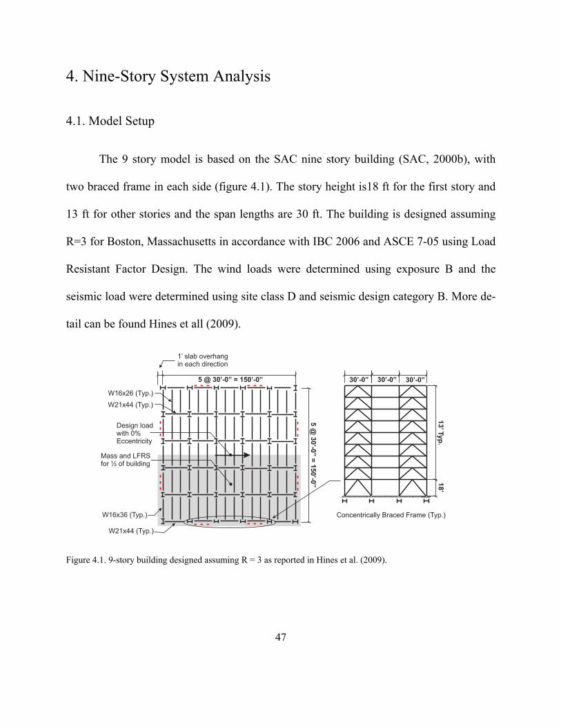
4. Nine-Story System Analysis
4.1. Model Setup
The 9 story model is based on the SAC nine story building (SAC, 2000b), with
two braced frame in each side (figure 4.1). The story height is18 ft for the first story and
13 ft for other stories and the span lengths are 30 ft. The building is designed assuming
R=3 for Boston, Massachusetts in accordance with IBC 2006 and ASCE 7-05 using Load
Resistant Factor Design. The wind loads were determined using exposure B and the
seismic load were determined using site class D and seismic design category B. More de-
tail can be found Hines et all (2009).
Figure 4.1. 9-story building designed assuming R = 3 as reported in Hines et al. (2009).
5 @ 30’-0” = 150’-0”
Design loadwith 0%Eccentricity
Mass and LFRSfor ½ of building
1’ slab overhangin each direction
13’Ty
p.
18’
30’-0” 30’-0” 30’-0”
5@
30’-0
”=
150’-0
”
Concentrically Braced Frame (Typ.)
W16x26 (Typ.)
W21x44 (Typ.)
W16x36 (Typ.)
W21x44 (Typ.)
48
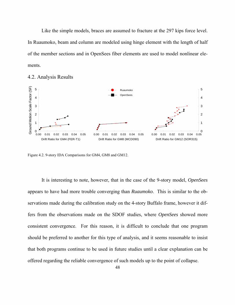
Like the simple models, braces are assumed to fracture at the 297 kips force level.
In Ruaumoko, beam and column are modeled using hinge element with the length of half
of the member sections and in OpenSees fiber elements are used to model nonlinear ele-
ments.
4.2. Analysis Results
Figure 4.2. 9-story IDA Comparisons for GM4, GM8 and GM12.
It is interesting to note, however, that in the case of the 9-story model, OpenSees
appears to have had more trouble converging than Ruaumoko. This is similar to the ob-
servations made during the calibration study on the 4-story Buffalo frame, however it dif-
fers from the observations made on the SDOF studies, where OpenSees showed more
consistent convergence. For this reason, it is difficult to conclude that one program
should be preferred to another for this type of analysis, and it seems reasonable to insist
that both programs continue to be used in future studies until a clear explanation can be
offered regarding the reliable convergence of such models up to the point of collapse.
0.00 0.01 0.02 0.03 0.04 0.05
Drift Ratio for GM4 (FER-T1)
0
1
2
3
4
5
Gro
und
Mot
ion
Sca
le F
acto
r (S
F)
Ruaumoko
OpenSees
0.00 0.01 0.02 0.03 0.04 0.05
Drift Ratio for GM8 (MCD090)
0.00 0.01 0.02 0.03 0.04 0.05
Drift Ratio for GM12 (SOR315)
0
1
2
3
4
5
49
In general, the 9-story model exhibited lower collapse resistance than the SDOF
model featured in Figure 3.15. There is, however, significant variation in collapse resis-
tance between ground motions. The primary difference between the 9-story model and
the SDOF model is the participation of higher mode effects. The nature of this participa-
tion, however, cannot be easily apprehended, because it does not correlate directly with
general observations of the ARS curves shown for the three ground motions in Figure
3.1. For instance, Figure 3.1 shows GM12 to have significant high frequency content,
whereas Figure 4.1 shows the 9-story structure with the highest collapse resistance under
GM12. This observation is consistent with comments made previously regarding such
systems (Hines et al. 2009, 2011) that their strength and stiffness discontinuities cause
some level of chaotic behavior that is sensitive not only to the shape of the response spec-
trum, but also the sequencing of pulses and other ground motion signal characteristics
that are not typically considered in suite selection.
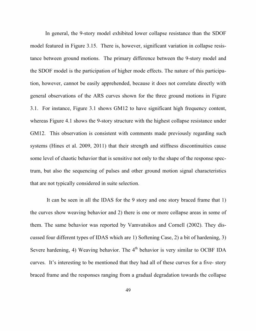
It can be seen in all the IDAS for the 9 story and one story braced frame that 1)
the curves show weaving behavior and 2) there is one or more collapse areas in some of
them. The same behavior was reported by Vamvatsikos and Cornell (2002). They dis-
cussed four different types of IDAS which are 1) Softening Case, 2) a bit of hardening, 3)
Severe hardening, 4) Weaving behavior. The 4th behavior is very similar to OCBF IDA
curves. It’s interesting to be mentioned that they had all of these curves for a five- story
braced frame and the responses ranging from a gradual degradation towards the collapse
50
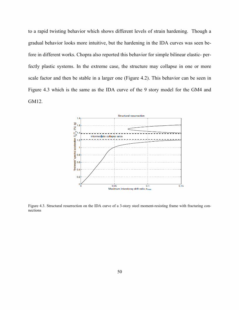
to a rapid twisting behavior which shows different levels of strain hardening. Though a
gradual behavior looks more intuitive, but the hardening in the IDA curves was seen be-
fore in different works. Chopra also reported this behavior for simple bilinear elastic- per-
fectly plastic systems. In the extreme case, the structure may collapse in one or more
scale factor and then be stable in a larger one (Figure 4.2). This behavior can be seen in
Figure 4.3 which is the same as the IDA curve of the 9 story model for the GM4 and
GM12.
Figure 4.3. Structural resurrection on the IDA curve of a 3-story steel moment-resisting frame with fracturing con-nections
51
5. Ultimate Moment Prediction Models for Type 2 Connections
5.1. Scope
5.1.1. Motivation
An understanding of connection behavior is essential to design safe and effective
reserve systems. A variety of connections have been tested experimentally since the
1930s, and multiple models have been developed to approximate the strength and stiff-
ness relationships of these connections. However, most of these models focus on initial
stiffness and stiffness degradation, while little has been determined about the strength of
the connections at failure. Kishi and Chen (1990) developed models that include ultimate
moment capacity predictions, but the theoretical basis of their equations does not provide
insight into the physical behavior of the connection. It is the goal of this study to find a
simple and intuitive model that can reasonably predict ultimate moment capacities of par-
tially restrained connections, specifically Type 2. Type 2 (top and seat with double web
angle) connections were chosen as the focus because of the large increase in moment ca-
pacity resulting from inexpensive and easy additions to simple connections.
The study estimates behavior of top and seat angle connections and double web
angle connections separately before developing predictions for Type 2 connections. Fig-
ure 5.1 shows these three connection types.
52
Figure 5.1. Connection types: (a) Top and seat angles; (b) Double web angles; (c) Type 2: top and seat with double
web angles.
5.1.2. Process
The following sections discuss prediction models by Kishi and Chen (1990) (he-
reafter referred to as Chen’s model) and Eurocode 3, Section 6.2.4. Chen’s model is theo-
retically based in structural mechanics, using Tresca and Drucker-Prager yield criterion to
determine ultimate resistance. Eurocode is the European Standard for calculating design
resistances. Eurocode does not provide a method for calculating capacity of web angles;
the study of double web angle and top and seat with double web angle connections in-
clude analyses only by Chen’s model and the simplified model.
Additionally, the author proposes a simplified model based on physical behavior.
Each model essentially follows a four-step process for determining the ultimate capacity
of a connection:
1. Determine relevant connection parameters.

53
2. Calculate the internal flexural span.
3. Determine shear resistance.
4. Calculate ultimate moment capacity.
The models are used to predict behavior of connections that have previously been
tested, and calculated results are compared to experimental.
The primary geometric parameter in predicting angle behavior in these models is
the span between the two plastic hinges that are formed during angle yield, referred to as
the internal flexural span, g2. The value of g2 is very important, as the prediction models
are highly sensitive to slight differences in length. Ultimate shear and moment predic-
tions are inversely related to g2. Each prediction model includes a different equation for
g2 that greatly influences the models’ results. Figure 5.2 compares g2 for the different
models. In reality, the flexural span changes across the leg of the angle, as shown in Fig-
ure 5.3. The computed g2 is an approximated equivalent length.
Figure 5.2. Internal flexural span, g2.
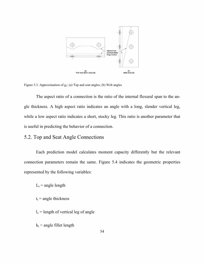
54
Figure 5.3. Approximation of g2: (a) Top and seat angles; (b) Web angles
The aspect ratio of a connection is the ratio of the internal flexural span to the an-
gle thickness. A high aspect ratio indicates an angle with a long, slender vertical leg,
while a low aspect ratio indicates a short, stocky leg. This ratio is another parameter that
is useful in predicting the behavior of a connection.
5.2. Top and Seat Angle Connections
Each prediction model calculates moment capacity differently but the relevant
connection parameters remain the same. Figure 5.4 indicates the geometric properties
represented by the following variables:
Lt = angle length
tt = angle thickness
lv = length of vertical leg of angle
kt = angle fillet length
55
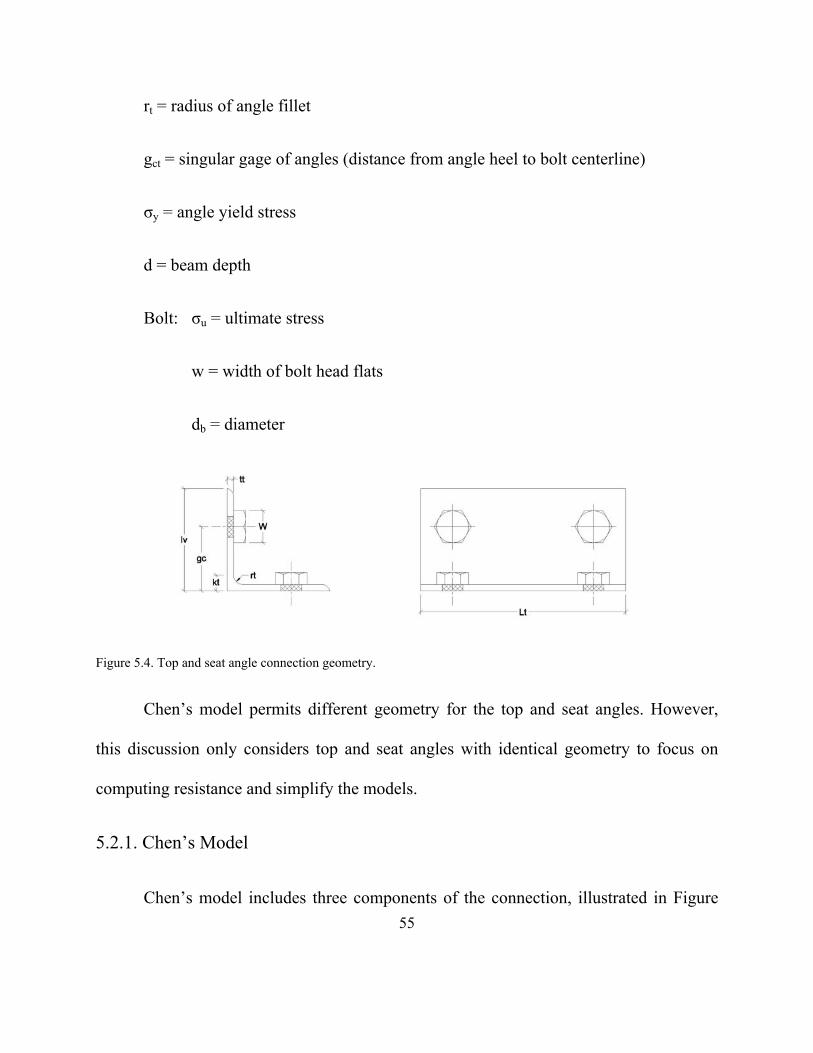
rt = radius of angle fillet
gct = singular gage of angles (distance from angle heel to bolt centerline)
σy = angle yield stress
d = beam depth
Bolt: σu = ultimate stress
w = width of bolt head flats
db = diameter
Figure 5.4. Top and seat angle connection geometry.
Chen’s model permits different geometry for the top and seat angles. However,
this discussion only considers top and seat angles with identical geometry to focus on
computing resistance and simplify the models.
5.2.1. Chen’s Model
Chen’s model includes three components of the connection, illustrated in Figure
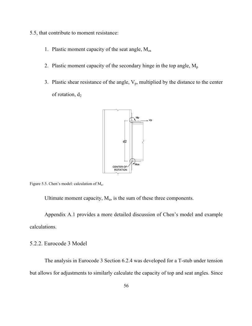
56
5.5, that contribute to moment resistance:
1. Plastic moment capacity of the seat angle, Mos
2. Plastic moment capacity of the secondary hinge in the top angle, Mp
3. Plastic shear resistance of the angle, Vp, multiplied by the distance to the center
of rotation, d2
Figure 5.5. Chen’s model: calculation of Mu.
Ultimate moment capacity, Mu, is the sum of these three components.
Appendix A.1 provides a more detailed discussion of Chen’s model and example
calculations.
5.2.2. Eurocode 3 Model
The analysis in Eurocode 3 Section 6.2.4 was developed for a T-stub under tension
but allows for adjustments to similarly calculate the capacity of top and seat angles. Since
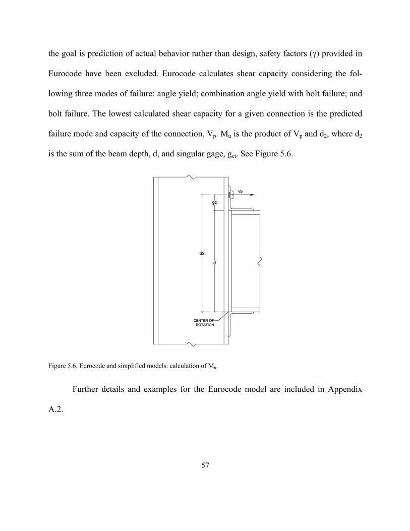
57
the goal is prediction of actual behavior rather than design, safety factors (γ) provided in
Eurocode have been excluded. Eurocode calculates shear capacity considering the fol-
lowing three modes of failure: angle yield; combination angle yield with bolt failure; and
bolt failure. The lowest calculated shear capacity for a given connection is the predicted
failure mode and capacity of the connection, Vp. Mu is the product of Vp and d2, where d2
is the sum of the beam depth, d, and singular gage, gct. See Figure 5.6.
Figure 5.6. Eurocode and simplified models: calculation of Mu.
Further details and examples for the Eurocode model are included in Appendix
A.2.
58
5.2.3. Simplified Model
The author developed the simplified model in an effort to predict ultimate moment
capacity through an intuitive sequence of calculations that makes physical sense to a
structural designer. The moment capacity of the angle provides the shear resistance, Vp,
for the overall connection, and Mu is calculated similar to the Eurocode model by multip-
lying Vp by d2 (Figure 5.6).
Refer to Appendix A.3 for a more comprehensive explanation and examples for
the simplified method.
5.2.4. Comparison of Models and Experimental Data
Table 5.1 displays moment capacities as predicted by each model and compares
them to experimental data by Kukreti et al (1999). Five specimens tested by Kukreti
failed due to their bolts. These specimens were excluded from this analysis since Chen’s
model and the simplified model only account for angle yield.
The Eurocode model consistently under-predicts the moment capacity of the con-
nections, with the lowest standard deviation of the three models. It may not be surprising
that the Eurocode model is the most conservative, since it is intended as a guide for de-
sign rather than a precise prediction of connection behavior. Chen’s model and the sim-
plified model both over-predict the experimental data by approximately 10% on average,
but the simplified model results are less precise, with a 0.42 standard deviation compared
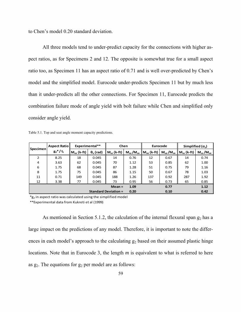
59
to Chen’s model 0.20 standard deviation.
All three models tend to under-predict capacity for the connections with higher as-
pect ratios, as for Specimens 2 and 12. The opposite is somewhat true for a small aspect
ratio too, as Specimen 11 has an aspect ratio of 0.71 and is well over-predicted by Chen’s
model and the simplified model. Eurocode under-predicts Specimen 11 but by much less
than it under-predicts all the other connections. For Specimen 11, Eurocode predicts the
combination failure mode of angle yield with bolt failure while Chen and simplified only
consider angle yield.
Table 5.1. Top and seat angle moment capacity predictions.
As mentioned in Section 5.1.2, the calculation of the internal flexural span g2 has a
large impact on the predictions of any model. Therefore, it is important to note the differ-
ences in each model’s approach to the calculating g2 based on their assumed plastic hinge
locations. Note that in Eurocode 3, the length m is equivalent to what is referred to here
as g2. The equations for g2 per model are as follows:
Mux (k‐ft) θu (rad) Muc (k‐ft) Muc /Mux Mue (k‐ft) Mue /Mux Mus (k‐ft) Mus /Mux
2 8.25 18 0.045 14 0.76 12 0.67 14 0.74
4 3.63 62 0.045 70 1.12 53 0.85 62 1.00
6 1.75 68 0.045 87 1.28 51 0.75 79 1.16
8 1.75 75 0.045 86 1.15 50 0.67 78 1.03
11 0.71 149 0.045 188 1.26 137 0.92 287 1.92
12 3.38 77 0.045 73 0.95 56 0.73 65 0.85
Mean = 1.09 0.77 1.12
0.20 0.10 0.42
*g2 in aspect ratio was calculated using the simplified model
**Experimental data from Kukreti et al (1999)
Simplified (σy)Experimental** Chen EurocodeSpecimen
Aspect Ratio
g2* / tt
Standard Deviation =
60
Chen’s Model
Eurocode 3 Model 0.8
Simplified Model
All three models confine g2 between the bolt centerline and angle fillet. (The Eu-
rocode model includes a small portion of the fillet (0.2ra) in g2.) Chen’s model and the
simplified model subtract half the bolt head width that holds the angle leg against the
column. The terms that include angle thickness in Chen’s and the Eurocode model are
approximations for the width of the plastic hinges. Overall, the Eurocode model generates
the longest g2 values, resulting in the lowest predictions, and Chen’s model generates the
shortest, which increase the predictions.
5.3. Double Web Angle Connections
The important connection parameters for web angle connections are listed below
and illustrated in Figure 5.7.
Lp = angle length
ta = angle thickness
ka = angle fillet length
gc = singular gage of angles
61
σy = angle yield stress
w = width of bolt head flats
Figure 5.7. Double web angle connection geometry.
Because of a web angle’s orientation, the connection shear distribution is not con-
stant along the length of the angle. Figure 5.8 shows the deformed shape of double web
angles, where it is obvious that the plastic hinge location varies.

62
Figure 5.8. Deformed double web angle connection.
5.3.1. Chen’s Model
For this connection type, Chen’s model refers to the variable flexural span length
as gy rather than the constant g2 discussed earlier. As seen in Figure 5.9, gy is a linear
function of the distance along the angle length, starting at the angle fillet ka (gy = 0) and
ending at the bolt centerline (gy = gc – ka). Appendix B.1 offers a more detailed explana-
tion of the theory behind gy, Chen’s shear distribution, and the resulting applied shear
force, Va.
63
Figure 5.9. Internal flexural span for double web angles.
The center of rotation is located at the base of the web angle. The moment arm
used to calculate Mu is the distance from the center of rotation to Va, and is calculated
based on the shear distribution geometry. Figure 5.10(a) shows the shear distribution and
moment arm assumed by Chen’s model.
5.3.2. Simplified Model
The simplified model calculates the internal flexural span g2 and maximum shear
capacity Vu the same as for top and seat angles. For the double web angles, however, the
shear is distributed triangularly along the length, as shown in Figure 5.10(b).
The assumed triangular shape of distribution determines the resultant shear force
Va and length of moment arm. Similar to Chen’s model, the center of rotation is located
at the base of the angle. More detail on the simplified model is included in Appendix B.2.
64
Figure 5.10. Assumed shear and moment resistance: (a) Chen’s Model; (b) Simplified Model.
5.3.3. Comparison of Models and Experimental Data
Abolmaali et al (2003) conducted tests on double web angles. Five test specimens
were excluded because they failed from web bearing rather than angle yield. Table 5.2
compares the remaining experimental data with capacity predictions by Chen’s model
and simplified model. Chen’s model greatly over-predicts the moment capacity by an av-
erage 86%. The simplified model over-predicts as well but by the relatively low average
of 11%, with the same standard deviation as Chen’s.
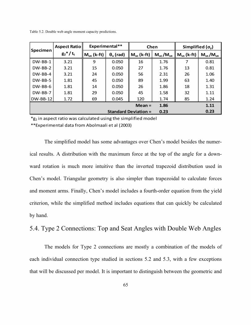
65
Table 5.2. Double web angle moment capacity predictions.
Mux (k‐ft) θu (rad) Muc (k‐ft) Muc /Mux Mus (k‐ft) Mus /Mux
DW‐BB‐1 3.21 9 0.050 16 1.76 7 0.81
DW‐BB‐2 3.21 15 0.050 27 1.76 13 0.81
DW‐BB‐4 3.21 24 0.050 56 2.31 26 1.06
DW‐BB‐5 1.81 45 0.050 89 1.99 63 1.40
DW‐BB‐6 1.81 14 0.050 26 1.86 18 1.31
DW‐BB‐7 1.81 29 0.050 45 1.58 32 1.11
DW‐BB‐12 1.72 69 0.045 120 1.74 85 1.24
Mean = 1.86 1.11
Standard Deviation = 0.23 0.23
*g2 in aspect ratio was calculated using the simplified model
**Experimental data from Abolmaali et al (2003)
SpecimenExperimental** Chen Simplified (σy)Aspect Ratio
g2* / tt
The simplified model has some advantages over Chen’s model besides the numer-
ical results. A distribution with the maximum force at the top of the angle for a down-
ward rotation is much more intuitive than the inverted trapezoid distribution used in
Chen’s model. Triangular geometry is also simpler than trapezoidal to calculate forces
and moment arms. Finally, Chen’s model includes a fourth-order equation from the yield
criterion, while the simplified method includes equations that can quickly be calculated
by hand.
5.4. Type 2 Connections: Top and Seat Angles with Double Web Angles
The models for Type 2 connections are mostly a combination of the models of
each individual connection type studied in sections 5.2 and 5.3, with a few exceptions
that will be discussed per model. It is important to distinguish between the geometric and
66
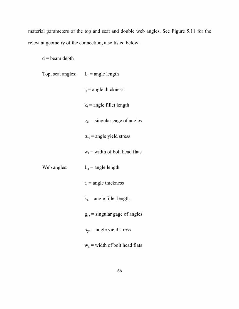
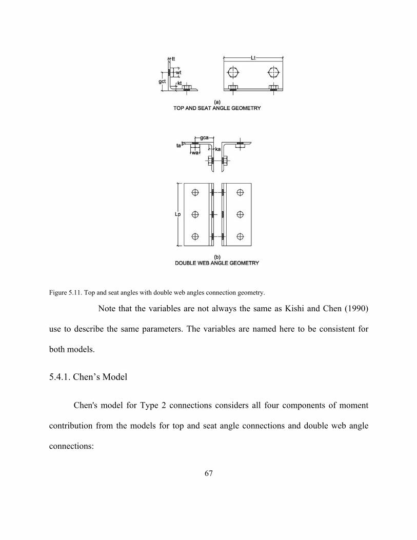
material parameters of the top and seat and double web angles. See Figure 5.11 for the
relevant geometry of the connection, also listed below.
d = beam depth
Top, seat angles: Lt = angle length
tt = angle thickness
kt = angle fillet length
gct = singular gage of angles
σyt = angle yield stress
wt = width of bolt head flats
Web angles: La = angle length
ta = angle thickness
ka = angle fillet length
gca = singular gage of angles
σya = angle yield stress
wa = width of bolt head flats
67
Figure 5.11. Top and seat angles with double web angles connection geometry.
Note that the variables are not always the same as Kishi and Chen (1990)
use to describe the same parameters. The variables are named here to be consistent for
both models.
5.4.1. Chen’s Model
Chen's model for Type 2 connections considers all four components of moment
contribution from the models for top and seat angle connections and double web angle
connections:

68
1. Plastic moment capacity of the seat angle, Mos
2. Plastic moment capacity of the secondary hinge in the top angle, Mpt
3. Plastic shear resistance of the top angle, Vpt, multiplied by the distance to the
center of rotation, d2
4. Plastic shear resistance of the double web angles, Vpa, multiplied by the dis-
tance to the center of rotation, d3
Calculations for including top and seat angle moment resistance into Chen’s mod-
el of the Type 2 connection do not change from section 5.1.1. The only difference from
section 5.2.1 for including the double web angles is the shift in location of the center of
rotation. The connection (including the web angles) rotates about a point halfway into the
horizontal leg of the seat angle. Thus, the moment arm for Vpa is extended and the mo-
ment resistance increases. Mu is calculated by summing all of the resistance offered by
top, seat, and both web angles. See Appendix C.1 for further investigation.
5.4.2. Simplified Model
As in Chen’s model, the simplified model does not change in approach to top and
seat angle capacity, and the double web angle capacity is changed by the shifted center of
rotation. Not only does the moment arm change, but the amount of shear resisted by the
angle increases as well. The reason for this is illustrated in Figure 5.12. The new shear
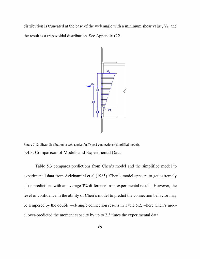
69
distribution is truncated at the base of the web angle with a minimum shear value, V1, and
the result is a trapezoidal distribution. See Appendix C.2.
Figure 5.12. Shear distribution in web angles for Type 2 connections (simplified model).
5.4.3. Comparison of Models and Experimental Data
Table 5.3 compares predictions from Chen’s model and the simplified model to
experimental data from Azizinamini et al (1985). Chen’s model appears to get extremely
close predictions with an average 3% difference from experimental results. However, the
level of confidence in the ability of Chen’s model to predict the connection behavior may
be tempered by the double web angle connection results in Table 5.2, where Chen’s mod-
el over-predicted the moment capacity by up to 2.3 times the experimental data.
70
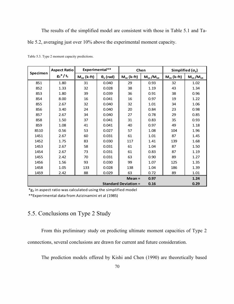
The results of the simplified model are consistent with those in Table 5.1 and Ta-
ble 5.2, averaging just over 10% above the experimental moment capacity.
Table 5.3. Type 2 moment capacity predictions.
Mux (k‐ft) θu (rad) Muc (k‐ft) Muc /Mux Mus (k‐ft) Mus /Mux
8S1 1.80 31 0.040 29 0.93 32 1.02
8S2 1.33 32 0.028 38 1.19 43 1.34
8S3 1.80 39 0.039 36 0.91 38 0.96
8S4 8.00 16 0.041 16 0.97 19 1.22
8S5 2.67 32 0.040 32 1.01 34 1.06
8S6 3.40 24 0.040 20 0.84 23 0.98
8S7 2.67 34 0.040 27 0.78 29 0.85
8S8 1.50 37 0.041 31 0.83 35 0.93
8S9 1.08 41 0.041 40 0.97 49 1.18
8S10 0.56 53 0.027 57 1.08 104 1.96
14S1 2.67 60 0.031 61 1.01 87 1.45
14S2 1.75 83 0.030 117 1.41 139 1.68
14S3 2.67 58 0.031 61 1.04 87 1.50
14S4 2.67 73 0.031 61 0.83 87 1.19
14S5 2.42 70 0.031 63 0.90 89 1.27
14S6 1.56 93 0.030 99 1.07 125 1.35
14S8 1.05 133 0.028 138 1.04 186 1.39
14S9 2.42 88 0.029 63 0.72 89 1.01
Mean = 0.97 1.24
0.16 0.29
*g2 in aspect ratio was calculated using the simplified model
**Experimental data from Azizinamini et al (1985)
Simplified (σy)
Standard Deviation =
SpecimenAspect Ratio
g2* / tt
Experimental** Chen
5.5. Conclusions on Type 2 Study
From this preliminary study on predicting ultimate moment capacities of Type 2
connections, several conclusions are drawn for current and future consideration.
The prediction models offered by Kishi and Chen (1990) are theoretically based
71
but do not always provide close or consistent results when compared with experimental
test data. Predictions for each connection type require solving fourth-order equations that
are not intuitive or efficient for practical use.
The simplified models proposed by the author do not claim to capture all of the
complex behavior occurring within a yielding connection, but relies upon basic under-
standing and a transparent process to approximate ultimate moment capacity. The models
need further refinement and over-predicted capacity by 10-15% the experimental results.
Investigating the Eurocode model was helpful as an additional comparison for top
and seat angle capacities, but did not include an analysis for we angle connections. Euro-
code was very conservative in its predictions, which might be attributed to its intended
use in design. The basic theory behind the development of the Eurocode in the angle
yield failure mode is similar to that of the simplified model.
A couple of issues have come up throughout the duration of this study.
1. None of the models currently account for strain hardening but depend on
yield stress for predicting ultimate capacities.
2. There is not sufficient data on top and seat angle, double web angle, or
Type 2 connections that were tested to failure to compare to the prediction
models.

72
3. Some of the test data that has been used did not report certain dimensions,
failure modes, or ultimate moments; these had to be assumed in order to
complete the study.
Further work must be done before the moment capacities of these connections are
able to be accurately predicted. Appendix D includes a comprehensive list of literature
that has been compiled for this study, including data that has not yet been used to cali-
brate the prediction models. This study should be expanded to incorporate the additional
data and consider other models once the literature has been reviewed. More experimental
tests with complete data sets must be conducted, and the prediction models must be re-
fined. However, it is clear that the types of connections discussed in this report all exhibit
moment capacities to be considered in further development of reserve system design me-
thodology.
73
6. Summary and Conclusions
The primary objective of this research is to develop confidence in collapse per-
formance prediction of low-ductility chevron braced frames as discussed by Hines et al.
(2009), who modeled these systems using Ruaumoko-2D (Carr 2004). The 2009 exposed
stiffness and strength discontinuities of these systems that raised the question of whether
consistent results could be expected between different software packages. For this rea-
son, the current validation study was engaged in order to compare Ruaumoko results with
results from large scale shake table tests and results from OpenSees (2006).
The best approach to develop confidence in modeling of collapse performance
would be to compare analytical results with large scale experimental results. In the ab-
sence of experimental data related to the collapse performance of low-ductility braced
frames, this study considered experimental work on a 4-story 1:8 scale moment frame at
the State University of New York (SUNY) in Buffalo (Lignos 2008). This moment frame
was tested to collapse, and therefore provided a good opportunity to calibrate OpenSees
and Ruaomoko models for prediction of side sway collapse under dynamic and P-D ef-
fects. Results showed that there is an acceptable correlation between Ruaomoko, Open-
Sees and experimental data.
The object of the next portion of this study (Chapter 3) was to demonstrate that
different software packages exhibit a high degree of consistency when used to model
74
regular, ductile systems. Several simple models were considered: 1) Cantilever, 2) 1-story
moment resistant frame (MRF), and 3) 1-story eccentric braced frame (EBF). The IDA
and displacement time history comparison for all ductile systems showed a good match
between OpenSees and Ruaomoko. These results coupled with the NEES Buffalo Frame
Study indicated that: 1) it is possible to model the nonlinear behavior of ductile systems
with high confidence and 2) there is a good match between maximum displacements for
all models but the residual displacements can vary significantly. Note that Yazgan and
Dazio (ETH Workshop, 2006) drew similar conclusions from comparative studies of
reinforced concrete structural walls modeled with OpenSees and Ruaumoko, and indi-
cated that it may be possible to address this issue
Based on these promising results, a one story chevron braced frame with re-
serve system was modeled in OpenSees and Ruaomoko. There were three main differ-
ences between the results of this system compared with ductile systems which were:
1) The IDA curve of this system showed weaving behavior while ductile systems
show softening or hardening behavior.
2) The correlation of IDA curves and time history displacement between Open-
Sees and Ruaomoko for this system was not as good as for ductile systems.
3) There were some convergence problems in the model obscuring whether non-
convergence represented physical collapse or some other numerical instability.
75
These results indicated that differences between OpenSees and Ruaomoko could
stem from the characteristic of brittle systems which is related to the brace fracture model
and sudden change of stiffness and strength of the systems. For these reasons, it is im-
portant to exercise caution when modeling such systems, and it is advisable to report re-
sults from more than one modeling approach or software package. Ultimately, it will be
very important to calibrate low-ductility braced frame models against experimental data.
In spite of the persisting uncertainties related to modeling these systems, it is still
possible to observe significant correlation between reserve capacity and collapse resis-
tance. Doubling the reserve capacity for the one story low-ductility braced frame in
Chapter 3 increased the collapse capacity significantly. Conversely, cutting the reserve
capacity in half reduced collapse capacity by more than a factor of 2.
The 9-story model was created in both software packages and the IDA curves
were compared. This study only considered the 9-story R3 model so far. Results indi-
cated that like one story braced frame model, the IDA curves showed weaving behavior
and there were some convergence problems in the model.
Finally, some of the basics of partially restrained connections were discussed
based on a literature review of bolted double web angle connections and bolted top and
seat angle connections used for Type II construction. This discussion emphasized the
need for analytical models that can reliably predict the ultimate moment capacity of par-
ticular connections. Such a model could facilitate the design of reserve systems based on
76
very simple considerations. Previous researchers have investigated such connections with
respect to their elastic performance under wind loads, and paid comparatively little atten-
tion to the moment-rotation performance of these connections up to the point of fracture.
Based on this observation, it is recommended to develop an experimental and analytical
program on these connections that focuses on their ultimate strength and deformation ca-
pacities.
Future work will include the following tasks:
- Further literature review of modeling issues, collapse behavior of building
structures, and experimental performance of PR connections.
- Experimental and analytical program to understand ultimate strength and de-
formation capacities of PR connections in terms of simple, physical models.
- Design a 9-story low ductility chevron braced frame with partially restrained
connections. This system will be designed with the assumption that moment
frames will take all the earthquake loads and the braced frames are for drift
control.
- Model this system in OpenSees and Ruaomoko and study the collapse beha-
vior.
- Investigate the possibility of incorporating IDA results from all scale factors
into reliability-based collapse assessment methods. Currently, only the scale

77
factor associated with collapse is used for collapse performance assessment,
and behavior at scale factors below the collapse level are ignored in the formal
assessment procedure.
- Model braces such that they don’t fracture at the same time, and investigate
other possible refinements to the system models, such as base plates, column
splices, etc.

78
References:
Abolmaali, A., A.R. Kukreti, & H. Razavi. (2003). Hysteresis behavior of semi-rigid
double web angle steel connections. Journal of Constructional Steel Research,
59:1057-1082.
Carr, A.J. (2004), Ruaumoko Manual Volumes 1 & 2, University of Canterbury, Christ-
church, New Zealand, 333 pp.
Chen, W.F. (2000). Practical Analysis for Semi-Rigid Frame Design. World Scientific,
Singapore.
Disque, R.O. (1976) Type 2 Construction with wind moment connections: a return to
simplicity, AISC.
Eurocode 3: Design of steel structures. Parts 1-8: Design of joints.
FEMA 355-D, (2000) State of the Art Report on Connection Performance. Federal Emer-
gency of Management Agency.
Geschwinder, L.F. and Disque, R.O. (2005) “Flexible Moment Connections for Unbraced
Frames Subject to Lateral Forces—A Return to Simplicity,” AISC Engineering
Journal, Second Quarter, pp. 99-112.
Hines, E.M., Appel, M.E. and Cheever, P.J. (2009) “Collapse Performance of Low-
Ductility Chevron Braced Steel Frames in Moderate Seismic Regions,” AISC En-
gineering Journal, 3rd Quarter, pp. 149-180.
79
Hines, E.M. and Fahnestock, L.A. (2010) “Design Philosophy for Steel Structures in
Moderate Seismic Regions,” 9th US National and 10th Canadian Conference on
Earthquake Engineering, EERI/CAEE, Toronto, Canada, July 25-29.
Hines, E.M., Baise, L.G. and Swift, S.S. (2011) “Ground Motion Suite Selection for
Eastern North America,” ASCE Journal of Structural Engineering, 137(3), March,
pp. 358-366.
Kishi, N., & W.F. Chen. (1990). Moment-rotation relations of semirigid connections with
angles. J. Struct. Eng., 116(7):1813-1834.
Kukreti, A.R., & A.S. Abolmaali. (1999). Moment rotation hysteresis behavior of top and
seat angle steel frame connections. J. Struct. Eng., 125(8):810-820.
Lignos, D.G. (2008) Sidesway Collapse of Deteriorating Structural Systems under Seis-
mic Excitations, Ph.D. Dissertation, Department of Civil and Environmental Engi-
neering, Stanford University, 457 pp.
Lignos, D.G., Krawinkler, H. and Whittaker, A.S. (2010) “Prediction and validation of
sidesway collapse of two scale models of a 4-story steel moment frame,” Earth-
quake Engineering and Structural Dynamics, Wiley Online Library, DOI:
10.1002/eqe.
Rodgers, J.E., Mahin,S.A.,(2004) Effects of Hysteretic Deterioration on Seismic Re-
sponse of Steel Moment Frames, Paper No.1581. 13th World conference on
Earthquake Engineering, Vancouver, B.C.,Canada.
80
Sorabella, S. (2006) Ground Motion Selection for Boston, Massachusetts, Masters Thesis,
Department of Civil and Environmental Engineering, Tufts University, Medford,
Massachusetts, 213 pp.
Uang, C. M. and Bertero, V. V. (1986) Earthquake Simulation Tests and Associated Stu-
dies of a 0.3-Scale Model of a Six-Story Concentrically Braced Steel Structure,
Report No. UCB/EERC-86/10, University of California, Berkeley, 363 pp.
Vamvastikos, D. and Cornell, C.A. (2002) “ Incremental Dynamic Analysis,” Earthquake
Engineering and Structural Dynamic.
Whittaker, A. S., Uang. C. M., and Bertero, V. V. (1990) An Experimental Study of the
Behavior of Dual Steel Systems, Report No. UCB/EERC-88/14, University of Cal-
ifornia, Berkeley.
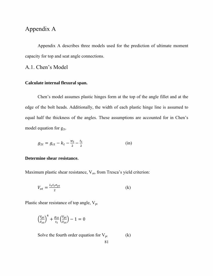
81
Appendix A
Appendix A describes three models used for the prediction of ultimate moment
capacity for top and seat angle connections.
A.1. Chen’s Model
Calculate internal flexural span.
Chen’s model assumes plastic hinges form at the top of the angle fillet and at the
edge of the bolt heads. Additionally, the width of each plastic hinge line is assumed to
equal half the thickness of the angles. These assumptions are accounted for in Chen’s
model equation for g2t.
(in)
Determine shear resistance.
Maximum plastic shear resistance, Vot, from Tresca’s yield criterion:
(k)
Plastic shear resistance of top angle, Vpt
1 0
Solve the fourth order equation for Vpt (k)
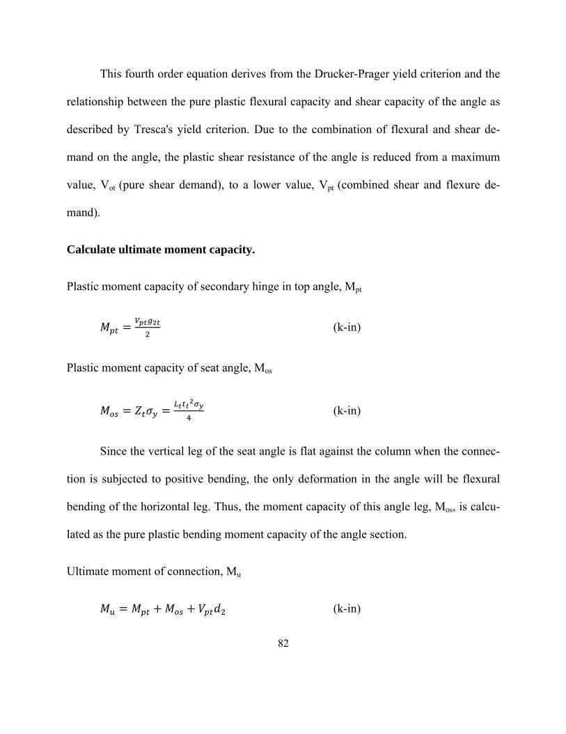
82
This fourth order equation derives from the Drucker-Prager yield criterion and the
relationship between the pure plastic flexural capacity and shear capacity of the angle as
described by Tresca's yield criterion. Due to the combination of flexural and shear de-
mand on the angle, the plastic shear resistance of the angle is reduced from a maximum
value, Vot (pure shear demand), to a lower value, Vpt (combined shear and flexure de-
mand).
Calculate ultimate moment capacity.
Plastic moment capacity of secondary hinge in top angle, Mpt
(k-in)
Plastic moment capacity of seat angle, Mos
(k-in)
Since the vertical leg of the seat angle is flat against the column when the connec-
tion is subjected to positive bending, the only deformation in the angle will be flexural
bending of the horizontal leg. Thus, the moment capacity of this angle leg, Mos, is calcu-
lated as the pure plastic bending moment capacity of the angle section.
Ultimate moment of connection, Mu
(k-in)

83
where (in)
The ultimate moment capacity is equal to the sum of the three moment contribu-
tions: Mpt, Mos, and Vptd2. These three contributions are derived from the moment resis-
tance of the top angle, the moment resistance of the seat angle, and the shear resistance of
the top angle, respectively. It should be noted that the majority of Mu is a result of Vptd2.
The variable d2 represents the distance from the center of rotation to the line of ac-
tion of Vpt. Chen's model assumes that the center of rotation is located half the thickness
of the seat angle below the bottom flange of the beam and that the line of action of Vpt
occurs at the top of the top angle fillet.
Example A.1
Determine relevant connection parameters.
Connection geometry from Kukreti et al (1999) - Specimen 6
Lt = 8.0 in
tt = 0.5 in
kt = 1.0 in
gct = 2.5 in
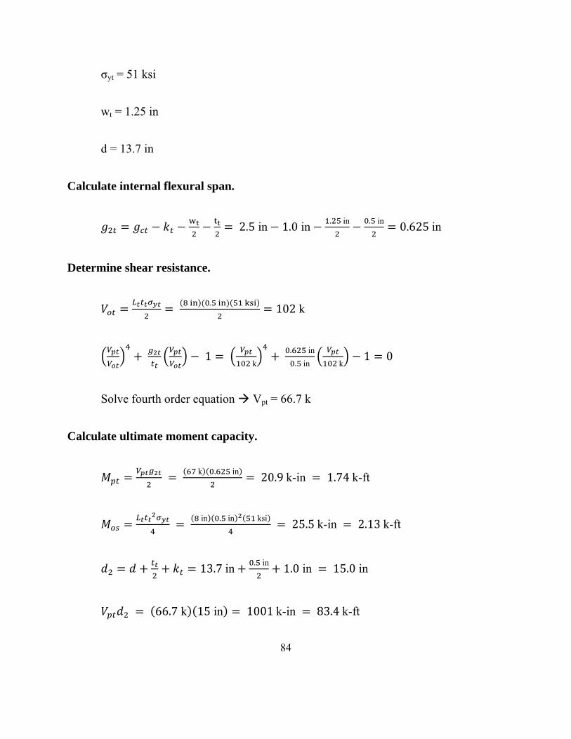
84
σyt = 51 ksi
wt = 1.25 in
d = 13.7 in
Calculate internal flexural span.
2.5 in 1.0 in. in . in 0.625 in
Determine shear resistance.
. 102 k
1 k
. in
. in k1 0
Solve fourth order equation Vpt = 66.7 k
Calculate ultimate moment capacity.
k . in 20.9 k-in 1.74 k-ft
in . in ksi 25.5 k-in 2.13 k-ft
13.7 in . in 1.0 in 15.0 in
66.7 k 15 in 1001 k-in 83.4 k-ft
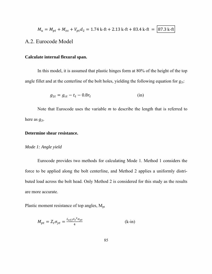
85
1.74 k-ft 2.13 k-ft 83.4 k-ft 87.3 k-ft
A.2. Eurocode Model
Calculate internal flexural span.
In this model, it is assumed that plastic hinges form at 80% of the height of the top
angle fillet and at the centerline of the bolt holes, yielding the following equation for g2t:
0.8 (in)
Note that Eurocode uses the variable m to describe the length that is referred to
here as g2t.
Determine shear resistance.
Mode 1: Angle yield
Eurocode provides two methods for calculating Mode 1. Method 1 considers the
force to be applied along the bolt centerline, and Method 2 applies a uniformly distri-
buted load across the bolt head. Only Method 2 is considered for this study as the results
are more accurate.
Plastic moment resistance of top angles, Mpt
(k-in)

86
where (in)
Leff is the adjusted angle length for the equivalent T-stub analysis.
Plastic shear resistance, Vpt
(k)
where (in)
1.25 (in)
Mode 2: Angle yield with bolt failure
Tension resistance of a single bolt, Ft
(k)
where k2 = 0.9 (Eurocode Table 3.4)
As = cross-sectional area of bolt (in2)
Plastic shear resistance, Vpt
∑ (k)
Mode 3: Bolt failure
Plastic shear resistance, Vpt
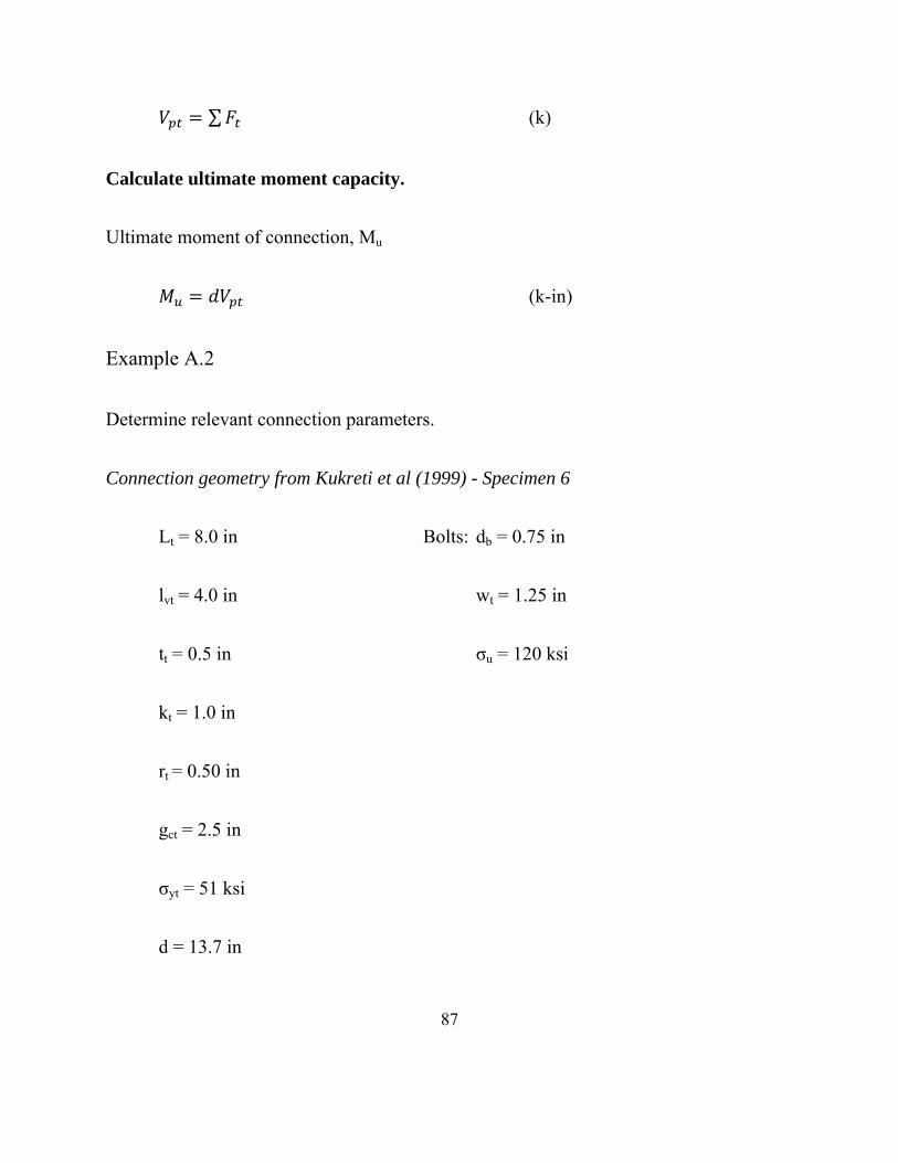
87
∑ (k)
Calculate ultimate moment capacity.
Ultimate moment of connection, Mu
(k-in)
Example A.2
Determine relevant connection parameters.
Connection geometry from Kukreti et al (1999) - Specimen 6
Lt = 8.0 in Bolts: db = 0.75 in
lvt = 4.0 in wt = 1.25 in
tt = 0.5 in σu = 120 ksi
kt = 1.0 in
rt = 0.50 in
gct = 2.5 in
σyt = 51 ksi
d = 13.7 in
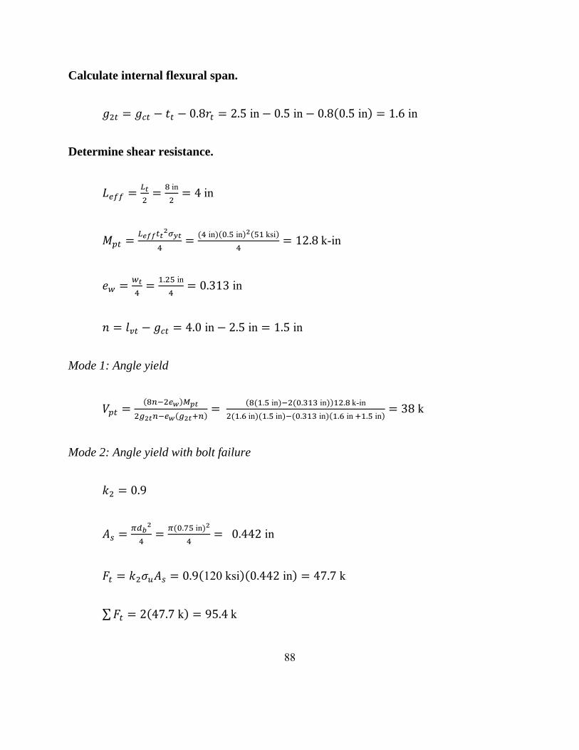
88
Calculate internal flexural span.
0.8 2.5 in 0.5 in 0.8 0.5 in 1.6 in
Determine shear resistance.
in 4 in
in . in ksi 12.8 k-in
. in 0.313 in
4.0 in 2.5 in 1.5 in
Mode 1: Angle yield
. in . in . k-in
. in . in . in . in . in38 k
Mode 2: Angle yield with bolt failure
0.9
. in 0.442 in
0.9 120 ksi 0.442 in 47.7 k
∑ 2 47.7 k 95.4 k
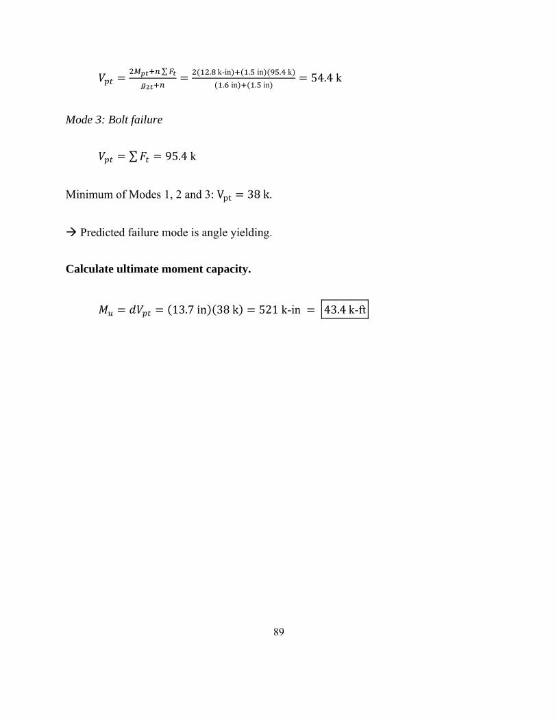
89
∑ . k-in . in . k
. in . in54.4 k
Mode 3: Bolt failure
∑ 95.4 k
Minimum of Modes 1, 2 and 3: V 38 k.
Predicted failure mode is angle yielding.
Calculate ultimate moment capacity.
13.7 in 38 k 521 k-in 43.4 k-ft
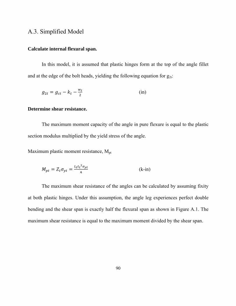
90
A.3. Simplified Model
Calculate internal flexural span.
In this model, it is assumed that plastic hinges form at the top of the angle fillet
and at the edge of the bolt heads, yielding the following equation for g2t:
(in)
Determine shear resistance.
The maximum moment capacity of the angle in pure flexure is equal to the plastic
section modulus multiplied by the yield stress of the angle.
Maximum plastic moment resistance, Mpt
(k-in)
The maximum shear resistance of the angles can be calculated by assuming fixity
at both plastic hinges. Under this assumption, the angle leg experiences perfect double
bending and the shear span is exactly half the flexural span as shown in Figure A.1. The
maximum shear resistance is equal to the maximum moment divided by the shear span.
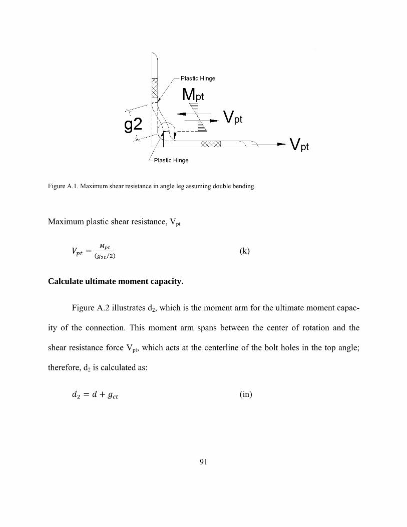
91
Figure A.1. Maximum shear resistance in angle leg assuming double bending.
Maximum plastic shear resistance, Vpt
⁄ (k)
Calculate ultimate moment capacity.
Figure A.2 illustrates d2, which is the moment arm for the ultimate moment capac-
ity of the connection. This moment arm spans between the center of rotation and the
shear resistance force Vpt, which acts at the centerline of the bolt holes in the top angle;
therefore, d2 is calculated as:
(in)
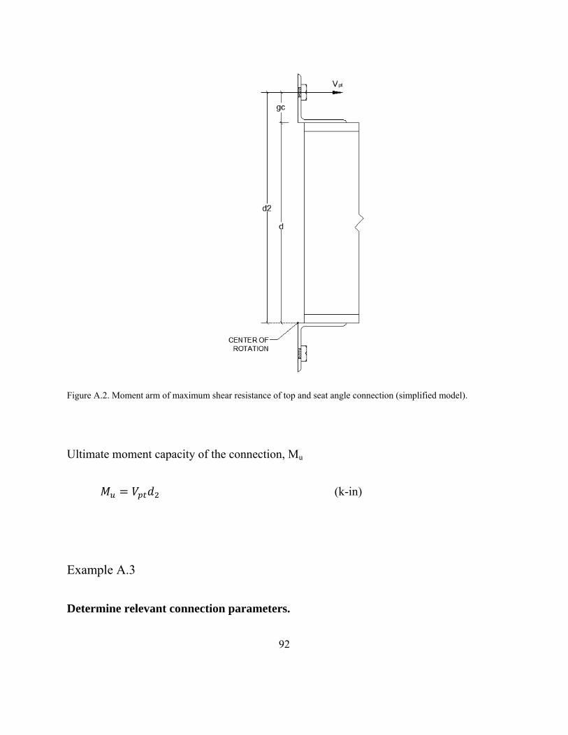
92
Figure A.2. Moment arm of maximum shear resistance of top and seat angle connection (simplified model).
Ultimate moment capacity of the connection, Mu
(k-in)
Example A.3
Determine relevant connection parameters.
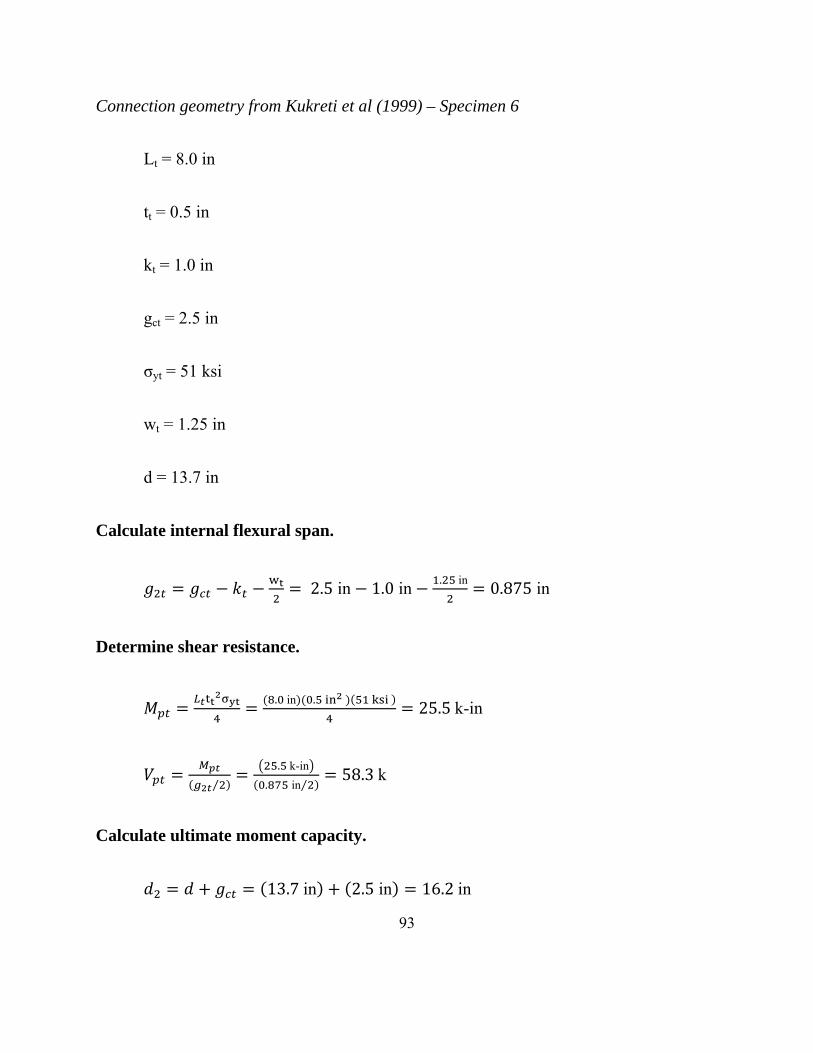
93
Connection geometry from Kukreti et al (1999) – Specimen 6
Lt = 8.0 in
tt = 0.5 in
kt = 1.0 in
gct = 2.5 in
σyt = 51 ksi
wt = 1.25 in
d = 13.7 in
Calculate internal flexural span.
2.5 in 1.0 in. in 0.875 in
Determine shear resistance.
. in . 25.5 k-in
⁄
. k-in
. in⁄58.3 k
Calculate ultimate moment capacity.
13.7 in 2.5 in 16.2 in

94
58.3 k 16.2 in 944 k-in 78.7 k-ft
Example A.4
Determine relevant connection parameters.
Connection geometry from Kukreti et al (1999) – Specimen 2
Lt = 8.0 in
tt = 0.375 in
kt = 0.875 in
gct = 4.5 in
σyt = 49 ksi
wt = 1.0625 in
d = 13.7 in
Calculate internal flexural span.
4.5 in 0.875 in. in 3.09 in
Determine shear resistance.
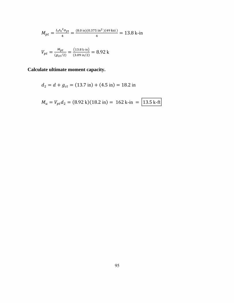
95
. in . 13.8 k-in
⁄
. k-in
. in⁄8.92 k
Calculate ultimate moment capacity.
13.7 in 4.5 in 18.2 in
8.92 k 18.2 in 162 k-in 13.5 k-ft
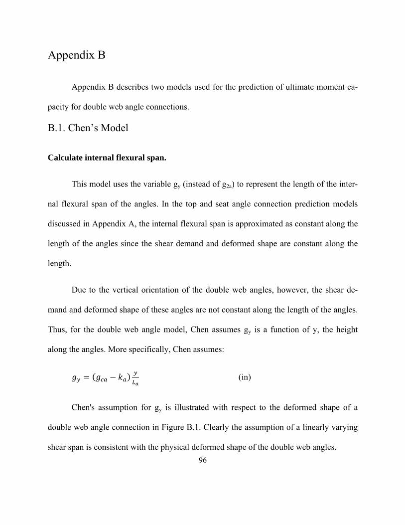
96
Appendix B
Appendix B describes two models used for the prediction of ultimate moment ca-
pacity for double web angle connections.
B.1. Chen’s Model
Calculate internal flexural span.
This model uses the variable gy (instead of g2a) to represent the length of the inter-
nal flexural span of the angles. In the top and seat angle connection prediction models
discussed in Appendix A, the internal flexural span is approximated as constant along the
length of the angles since the shear demand and deformed shape are constant along the
length.
Due to the vertical orientation of the double web angles, however, the shear de-
mand and deformed shape of these angles are not constant along the length of the angles.
Thus, for the double web angle model, Chen assumes gy is a function of y, the height
along the angles. More specifically, Chen assumes:
(in)
Chen's assumption for gy is illustrated with respect to the deformed shape of a
double web angle connection in Figure B.1. Clearly the assumption of a linearly varying
shear span is consistent with the physical deformed shape of the double web angles.
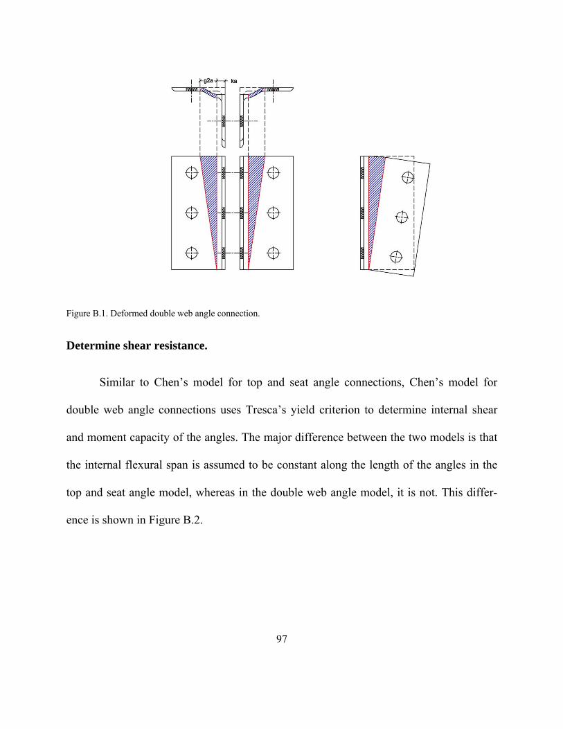
97
Figure B.1. Deformed double web angle connection.
Determine shear resistance.
Similar to Chen’s model for top and seat angle connections, Chen’s model for
double web angle connections uses Tresca’s yield criterion to determine internal shear
and moment capacity of the angles. The major difference between the two models is that
the internal flexural span is assumed to be constant along the length of the angles in the
top and seat angle model, whereas in the double web angle model, it is not. This differ-
ence is shown in Figure B.2.
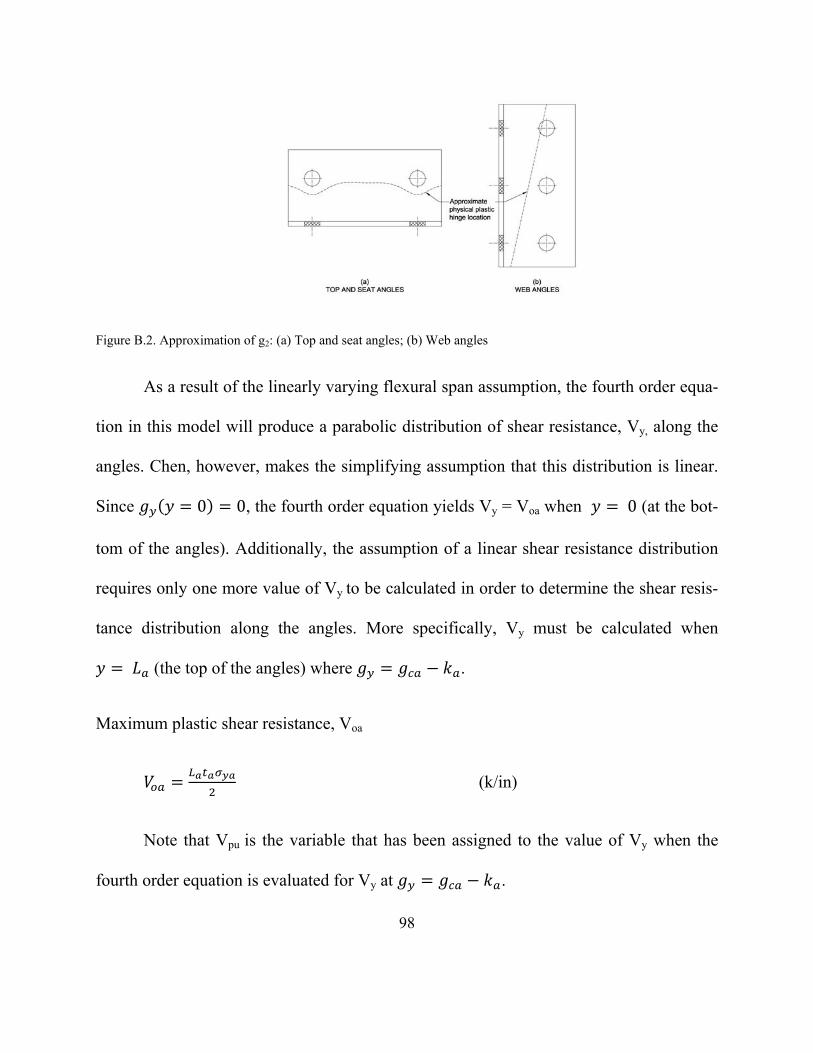
98
Figure B.2. Approximation of g2: (a) Top and seat angles; (b) Web angles
As a result of the linearly varying flexural span assumption, the fourth order equa-
tion in this model will produce a parabolic distribution of shear resistance, Vy, along the
angles. Chen, however, makes the simplifying assumption that this distribution is linear.
Since 0 0, the fourth order equation yields Vy = Voa when 0 (at the bot-
tom of the angles). Additionally, the assumption of a linear shear resistance distribution
requires only one more value of Vy to be calculated in order to determine the shear resis-
tance distribution along the angles. More specifically, Vy must be calculated when
(the top of the angles) where .
Maximum plastic shear resistance, Voa
(k/in)
Note that Vpu is the variable that has been assigned to the value of Vy when the
fourth order equation is evaluated for Vy at .
99
Minimum plastic shear resistance ( ), Vpu
1 0
Solve the fourth order equation for Vpu (k/in)
Total shear resistance of each web angle, Va
(k)
The resulting shear resistance in each web angle is an inverted trapezoidal distri-
bution with a maximum value Voa at the bottom of the angles and a minimum value Vpu
at the top of the angles. The total shear resistance of each web, Va, is equal to the area of
this trapezoidal distribution. This distribution is shown in Figure B.3.
Figure B.3. Assumed shear resistance of double web angles (Chen’s Model)
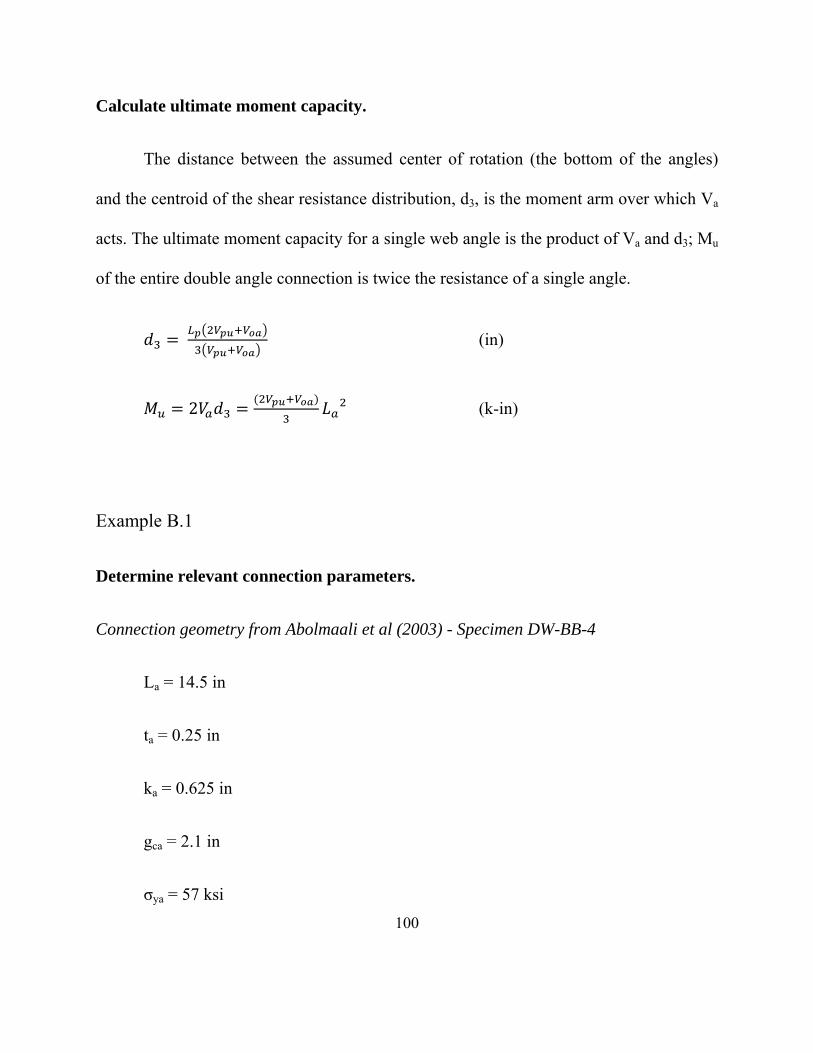
100
Calculate ultimate moment capacity.
The distance between the assumed center of rotation (the bottom of the angles)
and the centroid of the shear resistance distribution, d3, is the moment arm over which Va
acts. The ultimate moment capacity for a single web angle is the product of Va and d3; Mu
of the entire double angle connection is twice the resistance of a single angle.
(in)
2 (k-in)
Example B.1
Determine relevant connection parameters.
Connection geometry from Abolmaali et al (2003) - Specimen DW-BB-4
La = 14.5 in
ta = 0.25 in
ka = 0.625 in
gca = 2.1 in
σya = 57 ksi
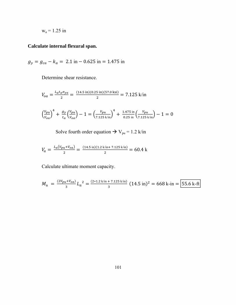
101
wa = 1.25 in
Calculate internal flexural span.
2.1 in 0.625 in 1.475 in
Determine shear resistance.
. . . 7.125 k/in
1. k/in
. in
. in . k/in1 0
Solve fourth order equation Vpu = 1.2 k/in
. in . k/in . k/in 60.4 k
Calculate ultimate moment capacity.
. k/in . k/in 14.5 in 668 k-in 55.6 k-ft
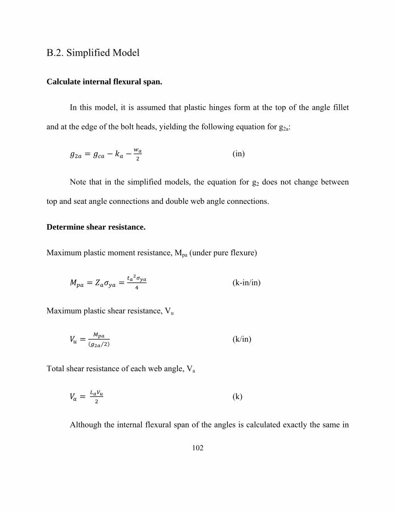
102
B.2. Simplified Model
Calculate internal flexural span.
In this model, it is assumed that plastic hinges form at the top of the angle fillet
and at the edge of the bolt heads, yielding the following equation for g2a:
(in)
Note that in the simplified models, the equation for g2 does not change between
top and seat angle connections and double web angle connections.
Determine shear resistance.
Maximum plastic moment resistance, Mpa (under pure flexure)
(k-in/in)
Maximum plastic shear resistance, Vu
⁄ (k/in)
Total shear resistance of each web angle, Va
(k)
Although the internal flexural span of the angles is calculated exactly the same in
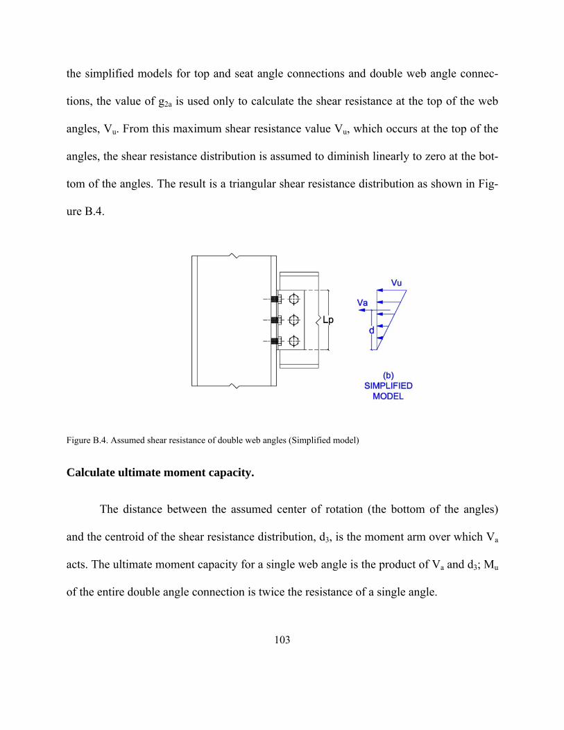
103
the simplified models for top and seat angle connections and double web angle connec-
tions, the value of g2a is used only to calculate the shear resistance at the top of the web
angles, Vu. From this maximum shear resistance value Vu, which occurs at the top of the
angles, the shear resistance distribution is assumed to diminish linearly to zero at the bot-
tom of the angles. The result is a triangular shear resistance distribution as shown in Fig-
ure B.4.
Figure B.4. Assumed shear resistance of double web angles (Simplified model)
Calculate ultimate moment capacity.
The distance between the assumed center of rotation (the bottom of the angles)
and the centroid of the shear resistance distribution, d3, is the moment arm over which Va
acts. The ultimate moment capacity for a single web angle is the product of Va and d3; Mu
of the entire double angle connection is twice the resistance of a single angle.
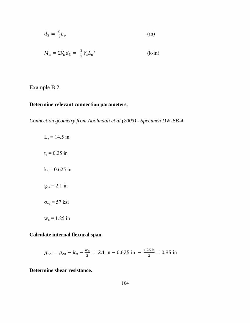
104
(in)
2 (k-in)
Example B.2
Determine relevant connection parameters.
Connection geometry from Abolmaali et al (2003) - Specimen DW-BB-4
La = 14.5 in
ta = 0.25 in
ka = 0.625 in
gca = 2.1 in
σya = 57 ksi
wa = 1.25 in
Calculate internal flexural span.
2.1 in 0.625 in . in 0.85 in
Determine shear resistance.
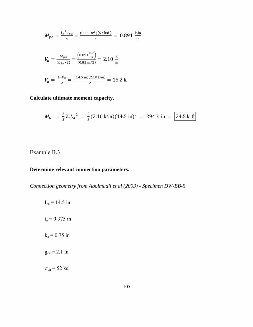
105
. 0.891 k-in
in
⁄
. k-inin
. in⁄2.10 k
in
. in . k/in 15.2 k
Calculate ultimate moment capacity.
2.10 k/in 14.5 in 294 k-in 24.5 k-ft
Example B.3
Determine relevant connection parameters.
Connection geometry from Abolmaali et al (2003) - Specimen DW-BB-5
La = 14.5 in
ta = 0.375 in
ka = 0.75 in
gca = 2.1 in
σya = 52 ksi

106
wa = 1.25 in
Calculate internal flexural span.
2.1 in 0.75 in . in 0.725 in
Determine shear resistance.
. 1.83 k-in
in
⁄
. k-inin
. in⁄5.04 k
in
. in . k/in 36.6 k
Calculate ultimate moment capacity.
14.5 in 9.67 in
5.04 k/in 14.5 in 707 k-in 59.0 k-ft

107
Appendix C
Appendix C describes two models used for the prediction of ultimate moment ca-
pacity for Type 2 connections.
C.1. Chen’s Model
Calculate internal flexural span.
(in) Top and seat angles
(in) Double web angles
Determine shear resistance.
Top and Seat Angles
Maximum plastic shear resistance, Vot (pure shear)
(k)
Plastic shear resistance, Vpt (shear and flexure)
1 0
Solve the fourth order equation for Vpt (k)
Double Web Angles
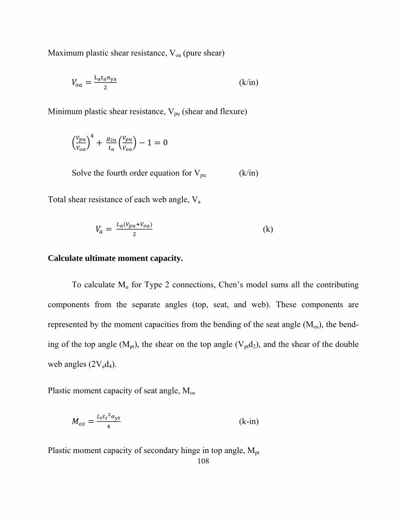
108
Maximum plastic shear resistance, Voa (pure shear)
L (k/in)
Minimum plastic shear resistance, Vpu (shear and flexure)
1 0
Solve the fourth order equation for Vpu (k/in)
Total shear resistance of each web angle, Va
(k)
Calculate ultimate moment capacity.
To calculate Mu for Type 2 connections, Chen’s model sums all the contributing
components from the separate angles (top, seat, and web). These components are
represented by the moment capacities from the bending of the seat angle (Mos), the bend-
ing of the top angle (Mpt), the shear on the top angle (Vptd2), and the shear of the double
web angles (2Vad4).
Plastic moment capacity of seat angle, Mos
(k-in)
Plastic moment capacity of secondary hinge in top angle, Mpt

109
(k-in)
Ultimate moment of connection, Mu
2 (k-in)
where (in)
(in)
The variable d2 describes the distance from the center of rotation to the line of ac-
tion of Vpt, and d4 is the distance from the center of rotation to Va. Vptd2 is the plastic
moment capacity of the primary hinge in the top angle. 2Vad4 is the plastic moment ca-
pacity of the double web angles.
Example C.1
Determine relevant connection parameters.
Connection geometry from Azizinamini et al (1985) - Specimen 8S4
d = 8.28 in
Top, seat angles: Lt = 6.0 in Web angles: La = 5.5 in

110
tt = 0.375 in ta = 0.25 in
kt = 0.875 in ka = 0.625 in
gct = 4.5 in gca = 2.59 in
σyt = 40.6 ksi σya = 40 ksi
wt = 1.25 in wa = 1.25 in
Calculate internal flexural spans.
4.5 in 0.875 . in . in 2.8125 in
2.59 in 0.625 in 1.965 in
Determine shear resistance.
Top and Seat Angles
. in . in . ksi 45.675 k
1. k
. in
. in . k1 0
Solve fourth order equation Vpt = 6.1 k
Double Web Angles
. in ksi 5 k/in

111
1 k/in
. in
. in . k1 0
Solve fourth order equation Vpu = 0.63 k/in
. in . k/in k/in 15.5 k
Calculate ultimate moment capacity.
. in . in . ksi 8.564 k-in 0.71 k-ft
k . in 8.4375 k-in 0.70 k-ft
8.28 in. in 0.875 in 9.3425 in
6.1 k 9.3425 in 57 k-in 4.75 k-ft
. in . k k
. k k
. in . in . in 3.62 in
2 2 15.5 k 3.62 in 112 k-in 9.35 k-ft
2 0.71 k-ft 0.70 k-ft 4.75 k-ft
9.35 k-ft = 15.5 k‐ft

112
C.2. Simplified Model
Calculate internal flexural span.
(in) Top and seat angles
(in) Double web angles
Determine shear resistance.
Top and Seat Angles
Maximum plastic moment resistance, Mpt
(k-in)
Plastic shear resistance, Vpt
⁄ (k)
Double Web Angles
The simplified model for Type 2 connections is essentially a combination of the
simplified models for top and seat angle connections and double web angle connections.
However, the centers of rotation for the top and seat angle connection and double web
angle connection are not located at the same point; the top and seat angle model assumes
a center of rotation within the heel of the seat angle, while the double web angle model
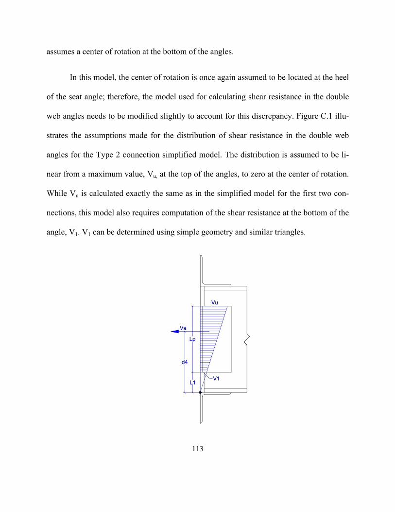
113
assumes a center of rotation at the bottom of the angles.
In this model, the center of rotation is once again assumed to be located at the heel
of the seat angle; therefore, the model used for calculating shear resistance in the double
web angles needs to be modified slightly to account for this discrepancy. Figure C.1 illu-
strates the assumptions made for the distribution of shear resistance in the double web
angles for the Type 2 connection simplified model. The distribution is assumed to be li-
near from a maximum value, Vu, at the top of the angles, to zero at the center of rotation.
While Vu is calculated exactly the same as in the simplified model for the first two con-
nections, this model also requires computation of the shear resistance at the bottom of the
angle, V1. V1 can be determined using simple geometry and similar triangles.
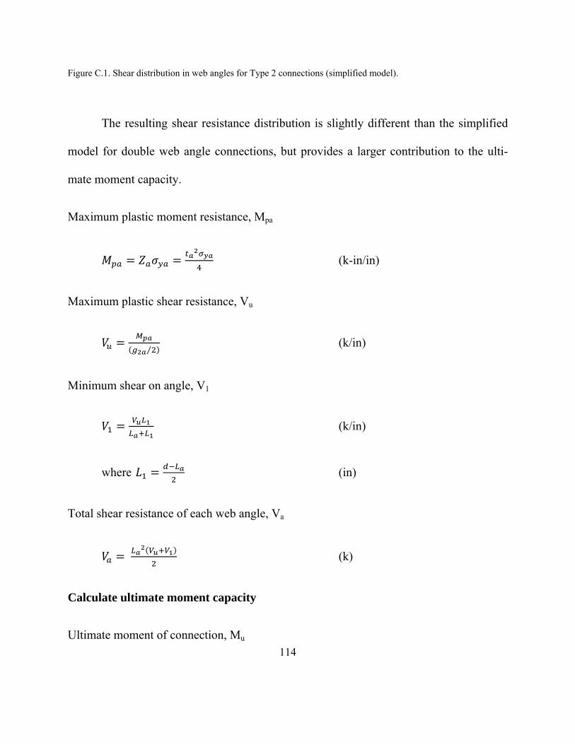
114
Figure C.1. Shear distribution in web angles for Type 2 connections (simplified model).
The resulting shear resistance distribution is slightly different than the simplified
model for double web angle connections, but provides a larger contribution to the ulti-
mate moment capacity.
Maximum plastic moment resistance, Mpa
(k-in/in)
Maximum plastic shear resistance, Vu
⁄ (k/in)
Minimum shear on angle, V1
(k/in)
where (in)
Total shear resistance of each web angle, Va
(k)
Calculate ultimate moment capacity
Ultimate moment of connection, Mu
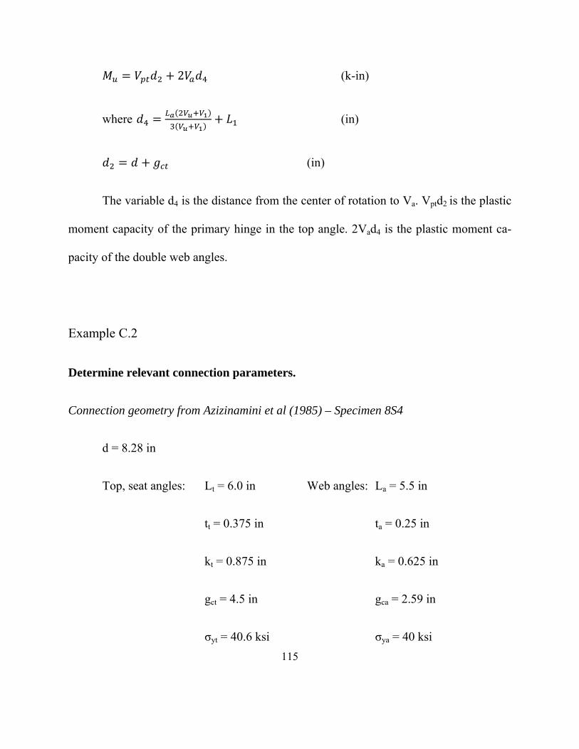
115
2 (k-in)
where (in)
(in)
The variable d4 is the distance from the center of rotation to Va. Vptd2 is the plastic
moment capacity of the primary hinge in the top angle. 2Vad4 is the plastic moment ca-
pacity of the double web angles.
Example C.2
Determine relevant connection parameters.
Connection geometry from Azizinamini et al (1985) – Specimen 8S4
d = 8.28 in
Top, seat angles: Lt = 6.0 in Web angles: La = 5.5 in
tt = 0.375 in ta = 0.25 in
kt = 0.875 in ka = 0.625 in
gct = 4.5 in gca = 2.59 in
σyt = 40.6 ksi σya = 40 ksi
116
wt = 1.25 in wa = 1.25 in
Calculate internal flexural spans.
4.5 in 0.875 in. in 3.00 in
2.59 in 0.625 in. in 1.34 in
Determine shear resistance.
Top and Seat Angles
. in . in . ksi 8.56 k-in
⁄
. k-in
. in⁄5.7 k
Double Web Angles
. 0.625 k-in
in
⁄
.
. in⁄0.932 k
in
. in . in 1.39 in
.kin
. in
. in . in0.188 k
117
. in .
kin
. kin 16.9 k
Calculate ultimate moment capacity.
8.28 in 4.5 in 12.8 in
5.7 k 12.8 in 73 k-in 6.0 k-ft
. in . k . k
. k . k1.39 in 4.75 in
2 2 16.9 k 4.75 in 160.6 k-in 13.4 k-ft
2 6.0 k-ft 13.4 k-ft 19.4 k-ft
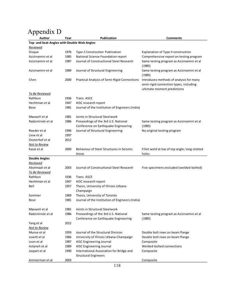
118
Appendix D
Author Year Publication Comments
Top‐ and Seat‐Angles with Double Web Angles
Reviewed
Disque 1976 Type 2 Construction Publication Explanation of Type II construction
Azizinamini et al 1985 National Science Foundation report Comprehensive report on testing program
Azizinamini et al 1987 Journal of Constructional Steel Research Same testing program as Azizinamini et al
(1985)
Azizinamini et al 1989 Journal of Structural Engineering Same testing program as Azizinamini et al
(1985)
Chen 2000 Practical Analysis of Semi‐Rigid Connections Introduces methods of analysis for many
semi‐rigid connection types, including
ultimate moment predictions
To Be Reviewed
Rathbun 1936 Trans. ASCE
Hechtman et al 1947 AISC research report
Bose 1981 Journal of the Institution of Engineers (India)
Maxwell et al 1981 Joints in Structural Steelwork
Radziminski et al 1986 Proceedings of the 3rd U.S. National
Conference on Earthquake Engineering
Same testing program as Azizinamini et al
(1985)
Roeder et al 1996 Journal of Structural Engineering No original testing program
Liew et al 1997
Oosterhof et al 2012
Not to Review
Kasai et al 2000 Behaviour of Steel Structures in Seismic
Areas
Fillet weld at toe of top angle; long‐slotted
holes
Double Angles
Reviewed
Abolmaali et al 2003 Journal of Constructional Steel Research Five specimens excluded (welded‐bolted)
To Be Reviewed
Rathbun 1936 Trans. ASCE
Hechtman et al 1947 AISC research report
Bell 1957 Thesis, University of Illinois Urbana‐
Champaign
Sommer 1969 Thesis, University of Toronto
Bose 1981 Journal of the Institution of Engineers (India)
Maxwell et al 1981 Joints in Structural Steelwork
Radziminski et al 1986 Proceedings of the 3rd U.S. National
Conference on Earthquake Engineering
Same testing program as Azizinamini et al
(1985)
Yang et al 2012
Not to Review
Munse et al 1959 Journal of the Structural Division Double bolt rows on beam flange
Lewitt et al 1966 University of Illinois Urbana‐Champaign Double bolt rows on beam flange
Leon et al 1987 AISC Engineering Journal Composite
Astaneh et al 1989 AISC Engineering Journal Welded‐bolted connections
Jaspart et al 1990 International Association for Bridge and
Structural Engineers
Composite
Ammerman et al 2003 Composite
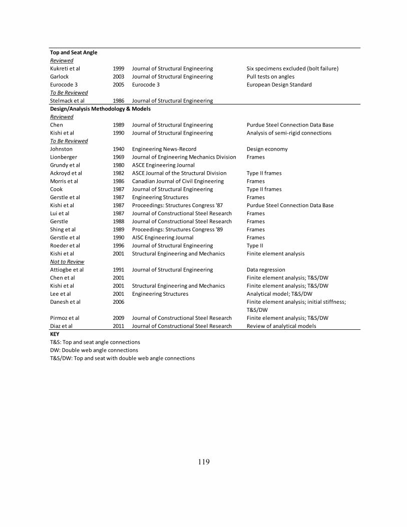
119
Top and Seat Angle
Reviewed
Kukreti et al 1999 Journal of Structural Engineering Six specimens excluded (bolt failure)
Garlock 2003 Journal of Structural Engineering Pull tests on angles
Eurocode 3 2005 Eurocode 3 European Design Standard
To Be Reviewed
Stelmack et al 1986 Journal of Structural Engineering
Design/Analysis Methodology & Models
Reviewed
Chen 1989 Journal of Structural Engineering Purdue Steel Connection Data Base
Kishi et al 1990 Journal of Structural Engineering Analysis of semi‐rigid connections
To Be Reviewed
Johnston 1940 Engineering News‐Record Design economy
Lionberger 1969 Journal of Engineering Mechanics Division Frames
Grundy et al 1980 ASCE Engineering Journal
Ackroyd et al 1982 ASCE Journal of the Structural Division Type II frames
Morris et al 1986 Canadian Journal of Civil Engineering Frames
Cook 1987 Journal of Structural Engineering Type II frames
Gerstle et al 1987 Engineering Structures Frames
Kishi et al 1987 Proceedings: Structures Congress '87 Purdue Steel Connection Data Base
Lui et al 1987 Journal of Constructional Steel Research Frames
Gerstle 1988 Journal of Constructional Steel Research Frames
Shing et al 1989 Proceedings: Structures Congress '89 Frames
Gerstle et al 1990 AISC Engineering Journal Frames
Roeder et al 1996 Journal of Structural Engineering Type II
Kishi et al 2001 Structural Engineering and Mechanics Finite element analysis
Not to Review
Attiogbe et al 1991 Journal of Structural Engineering Data regression
Chen et al 2001 Finite element analysis; T&S/DW
Kishi et al 2001 Structural Engineering and Mechanics Finite element analysis; T&S/DW
Lee et al 2001 Engineering Structures Analytical model; T&S/DW
Danesh et al 2006 Finite element analysis; initial stiffness;
T&S/DW
Pirmoz et al 2009 Journal of Constructional Steel Research Finite element analysis; T&S/DW
Diaz et al 2011 Journal of Constructional Steel Research Review of analytical models
KEY
T&S: Top and seat angle connections
DW: Double web angle connections
T&S/DW: Top and seat with double web angle connections