Common Trends and Common Cycles in Latin America:

A 2-Step Versus a ”Zigzag” Approach

Alain Hecq

University of Maastricht

Department of Quantitative Economics

P.O.Box 616

6200 MD Maastricht

The Netherlands

E-mail: a.hecq@ke.unimaas.nl

Homepage: www.personeel.unimaas.nl/a.hecq

March 31, 2005

Abstract

We are interested in determining the number of common trends and common cycles in the

gross domestic product of a set of Latin American countries. In order to unravel these two types

of common features on homogeneous and reasonably good series, we should rely on annual data.

Hence, in a time series framework, the number of variables is relatively large compared to the

number of observations to blindly trust the asymptotics. We propose to use an iterative strategy

that maximizes the likelihood function by successively imposing long and short-run restrictions until

convergence is achieved. Monte Carlo simulations stress advantages of this ”zigzag” approach over

the two-step one.

Keywords : Cointegration, Common cyclical feature, Monte Carlo, output growth, information

criteria.

JEL Classification : C32

1

1 INTRODUCTION

Cointegration techniques are now routinely applied by economists to extract r meaningful long-run

relationships among a set of n non-stationary time series yt = (y1t, . . . ynt)0. Interpreting the issue in

its dual form, this means there also exist n− r common trends, hence only n− r common permanentshocks driving the economy. To evaluate the presence of such long-run co-movements, the Johansen

maximum likelihood approach (1995 inter alia) based on Anderson’s results (e.g. 1984), is widely

used. In practice, after choosing the relevant series one needs (i) to select p, the lag length of the

finite order VAR generating the multivariate process yt, (ii) to find the deterministic terms, (iii) to

determine the cointegrating rank and quite often (iv) to restrict the cointegrating space. The literature

has shown that none of these steps is trivial. Next, the non stationary VAR is rewritten in its VECM

representation, ready for the discussion about its economic content, for the study of short and long-run

causality, for the analysis of the reduced number of shocks, for forecasting or for impulse response

analyses.

Beyond cointegration, a number of papers have concentrated on modelling the common serial cor-

relation feature among stationary time series. Indeed, alike cointegration is associated with long-run

relationships, common dynamics are a sign of co-movements in the short-run. The presence of common

propagation mechanisms, namely the so called common cycles, allows to extract common transitory

shocks that can often be linked to business cycle co-movements. At least this is the case for the

multivariate Beveridge-Nelson decomposition because the reduced number of transitory shocks is, in

the Gonzalo-Granger (1995) decomposition, inherent to the presence of cointegration. However this

is due to the fact that the Gonzalo-Granger decomposition underlies the presence of common cycles

(Proietti 1997; Hecq, Palm and Urbain 2000). Additional advantages of considering these short-run

restrictions are the large reduction of the number of parameters that need to be estimated and their

role for forecasting (see Vahid and Issler 2002 and Hecq, Palm and Urbain 2005 on this latter issue).

This being said, this note stresses another advantage of considering short-run co-movements, namely

the improvement of the small sample behavior of cointegration tests thanks to additional restrictions.

Several studies comment on the poor performance of the asymptotic Johansen test in small samples

(see inter alia Ho and Sorensen 1996; Gonzalo and Pitarakis 1999; Cheung and Lai 1993; Soderlind

2

and Vredin 1996; Jacobson, Vredin and Warne 1998 ). Most of the existing Monte Carlo simulations

point out that the dimension of the system for a given sample size may pose a problem, since the

number of parameters in VAR models grows very large as the dimension increases. It emerges that

likelihood ratio tests are often too liberal, which leads to overestimating the number of cointegrating

vectors r in empirical works. Likewise difficulties often arise when the lag length is either over or under

parametrized. Small sample corrections (a la Reinsel and Ahn 1992, for instance) may be helpful,

but in practice they often lead to underestimate r. Indeed, the distortion is non monotone with the

number of variables (Ho and Sorensen 1996). Johansen (2002) has proposed a correction factor to

circumvent this problem. An alternative solution is to use a bootstrap procedure such as in Fachin

(2000) or Harris and Judge (1998). Fachin and Omtzigt (2002) compare these two latter methods

and find that even though both do better than asymptotic tests, they still suffer from size distortions.

Concerning common dynamics, only few Monte Carlo results are available (see Beine and Hecq 1998;

Hecq 1998; Candelon, Hecq and Verschoor 2005). From these studies it emerges that common feature

test statistics are strongly sensitive to misspecifications such as the presence of seasonality, conditional

heteroskedasticity, outliers, aggregation.

Obviously, as far as both long-run and short-run co-movements are of interest for the researcher, a

natural practice consists in first estimating superconsistently the cointegrating vectors. In a subsequent

step, it will be easy to perform a test for common serial correlation by considering the cointegrating

relationships as given (see Vahid and Engle 1993). This is what we call the 2-step approach. The

drawback of the latter procedure is that a misleading inference about the cointegrating rank in the

first step may damage the subsequent analysis about common cycles (Hecq, Palm and Urbain 2005).

To try to improve the 2-step approach, this article evaluates whether an iterative procedure would

be helpful both for cointegration and common feature test statistics. In practice however, the cost of

implementing this more complicated procedure must be evaluated with the expected benefits. Overall,

simple adjustments for the degrees of freedom and the use of information criteria are helpful ”cheap”

alternatives.

The structure of this paper is as follows. Section 2 recalls the definitions. Section 3 describes the

test statistics. We show how to implement the approach that consists in switching between long-run

and short-run restrictions. Section 4 summarizes Monte Carlo results. Section 5 demonstrates the

3

use of these tests in a study of co-movements among the gross domestic products of six Latin American

countries for the period 1950-2002. A final section concludes.

2 MODEL REPRESENTATION AND DEFINITIONS

We consider Π(L)yt = ΘDt + εt the n-dimensional vector autoregressive model of order p for the I(1)

variables yt = (y1t, . . . ynt)0, i.e.

yt = ΘDt +Π1yt−1 + . . .+Πpyt−p + εt, t = 1, ..., T, (1)

for fixed values of y−p+1, ..., y0 and where Π(L) = In−Π1L− . . .−ΠpLp; Dt is a vector of deterministicterms, and the disturbances εt are NIID(0,Ω). Let us assume that rank(Π(1)) = r, 0 < r < n,

so that Π(1) can be expressed as Π(1) = −αβ0 , with α and β both (n × r) matrices of full columnrank r and that the characteristic equation |Π(z)| = 0 has n − r roots equal to 1 and all other rootsoutside the unit circle. The process yt is then cointegrated of order (1,1). The columns of β span the

space of cointegrating vectors, and the elements of α are the corresponding adjustment coefficients or

factor loadings. Decomposing the matrix lag polynomial Π(L) = Π(1)L + Γ(L)(1 − L), and defining∆ = (1− L), we obtain the vector error correction model

∆yt = ΘDt + αβ0yt−1 +

p−1Xj=1

Γj∆yt−j + εt, t = 1, . . . , T, (2)

where Γ0 = In, Γj = −Ppk=j+1Πk (j = 1, . . . , p− 1).

Serial correlation common feature (SCCF hereafter, see Engle and Kozicki 1993) holds for the

VECM in (2), if there exists a (n × s) matrix δ, whose columns span the cofeature space, such that

δ0(∆yt − ΘDt) = δ0εt is a s-dimensional zero mean vector innovation process with respect to the

information available at time t. Consequently, SCCF arises if there exists a matrix δ such that the

conditions δ0Γj = 0(s×n), j = 1 . . . p − 1 and δ

0Π(1) = −δ0αβ0 = 0(s×n) are jointly satisfied. Let us

denote a (n(p− 1)+ r)× 1 vector Wt−1 = [∆y0t−1, . . . ,∆y0t−p+1, y0t−1β]0and a n× (n(p− 1)+ r) matrix

4

Φ = [Γ1, . . . ,Γp−1,α], so that (2) has the factor representation

∆yt = ΘDt +ΦWt−1 + εt, t = 1, ..., T. (3)

Under SCCF, Φ is of reduced rank n− s and can be written as Φ = A[F1, . . . , Fp−1, Fp] = AF, whereA is n× (n− s) full column rank matrix and F is (n− s)× (n(p− 1) + r). δ0AFWt−1 = 0 means that

δ ∈ sp(A⊥) where sp denotes the space spanning by the columns of a matrix a A⊥, the orthogonalcomplement of A such that A

0A⊥ = 0 with rank(A⊥)= n − s and rank(A : A⊥)= n. Consequently,

as pointed out by Vahid and Engle (1993), in an n−dimensional I(1) vector process yt with r < n

cointegrating vectors, if the elements of yt have common cyclical features (given by ft = FWt−1) there

can be at most n−r linearly independent cofeature vectors that eliminate the common cyclical featuressince the cofeature matrix must lie in sp(α⊥). SCCF implies that s ≤ n − r (or r + s ≤ n) and thatthe common dynamic factors ft consist of linear combinations of the elements of Wt−1.

This set of long and short-run restrictions gives rise to a full description of the common trends and

cycles in yt. Indeed, from the Wold representation of the stationary process ∆yt and focussing on the

Beveridge-Nelson decomposition (ignoring deterministic terms for simplicity) we have

∆yt = C(L)εt,

= C(1)εt +∆C∗(L)εt, (4)

with C(L) = In +∞Pi=1CiL

i and∞Pj=1

j|Cj | < ∞ and C∗i = −∞Pj>iCj for all i. Integrate both sides of (4)

we obtain

yt = C(1)tPj=1

εj + C∗(L)εt,

= Trends+ Cycles.

These trends and cycles will be common to the series depending on the rank of the matrices C(1) and

C∗(L). Under cointegration rank(C(1)) = n− r and we know that the n− r common stochastic trends

5

α⊥tPj=1

εj are annihilated by β because β0C(1) = 0. Similarly, under SCCF, C∗(L) is of reduced rank

n− s and these n− s common cycles are such that δ0C∗(L) = 0 (see inter alia Issler and Vahid 2001).When cycles are not perfectly synchronized, alternative specifications have been proposed by Vahid

and Engle (1997) or Cubadda and Hecq (2001). These two latter models have the advantage to have

a nice interpretation in terms of delays of adjustment to shocks in the multivariate Beveridge-Nelson

representation. However, alike SCCF they are sensitive to misspecifications made on the determination

of the cointegrating rank. This is the reason why we consider the weak form common cycle specification

(WF hereafter, see Hecq, Palm and Urbain 2000, 2005) which is more robust to the choice of r.

Indeed, we have seen that the determination of the cointegrating space in the first step (possibly

misspecified) bounds the number of SCCF cofeature vectors. Instead, in the WF we have under the

null δ0(∆yt − ΘDt) = δ∗0β0yt−1 + δ0εt where δ∗0 = δ0α. We analogously define an n(p − 1) × 1 vector

Zt−1 = [∆y0t−1, . . . ,∆y0t−p+1]0and the n× n(p− 1) matrix Φ∗ = [Γ1, . . . ,Γp−1], so that (2) becomes

∆yt = ΘDt + αβ0yt−1 +Φ∗Zt−1 + εt, t = 1, ..., T, (5)

If Φ∗ is of reduced rank n−s it can be written as Φ∗ = A∗[F ∗1 , . . . , F ∗p−1] = A∗F ∗, where A∗ is n×(n−s)full column rank matrix and F ∗ is (n− s)×n(p− 1) such that δ0A∗F ∗Zt−1 = 0. The matrix δ must liein sp(A∗⊥) but not necessarily in sp(α⊥) and consequently we can have s > n− r weak form cofeature

vectors.

Another interesting advantage of jointly considering cointegration and WF restrictions arises when

working with transformed VAR models. To obtain this latter representation, let us denote C = (β :M)0

the n× n nonsingular matrix where M = (0(n−r)×r I(n−r)) is the selection matrix such that M 0∆yt =

∆y†t . Premultiplying both sides of the VECM in (2) by C we get CΓ(L)∆yt = Cαβ0yt−1+Cεt or if we

develop and rearrange the first block by putting −β0yt−1 in the right-hand-side

β0yt = (Ir + β0α)β0yt−1 + β0Γ(L)∆yt−1 + β0εt, (6)

∆y†t = (Mα)β0yt−1 + Γ(L)∆y†t−1 +Mεt, (7)

where Γ(L) = Γ(L) − In. This representation emphasize the need of an accurate estimation on the

6

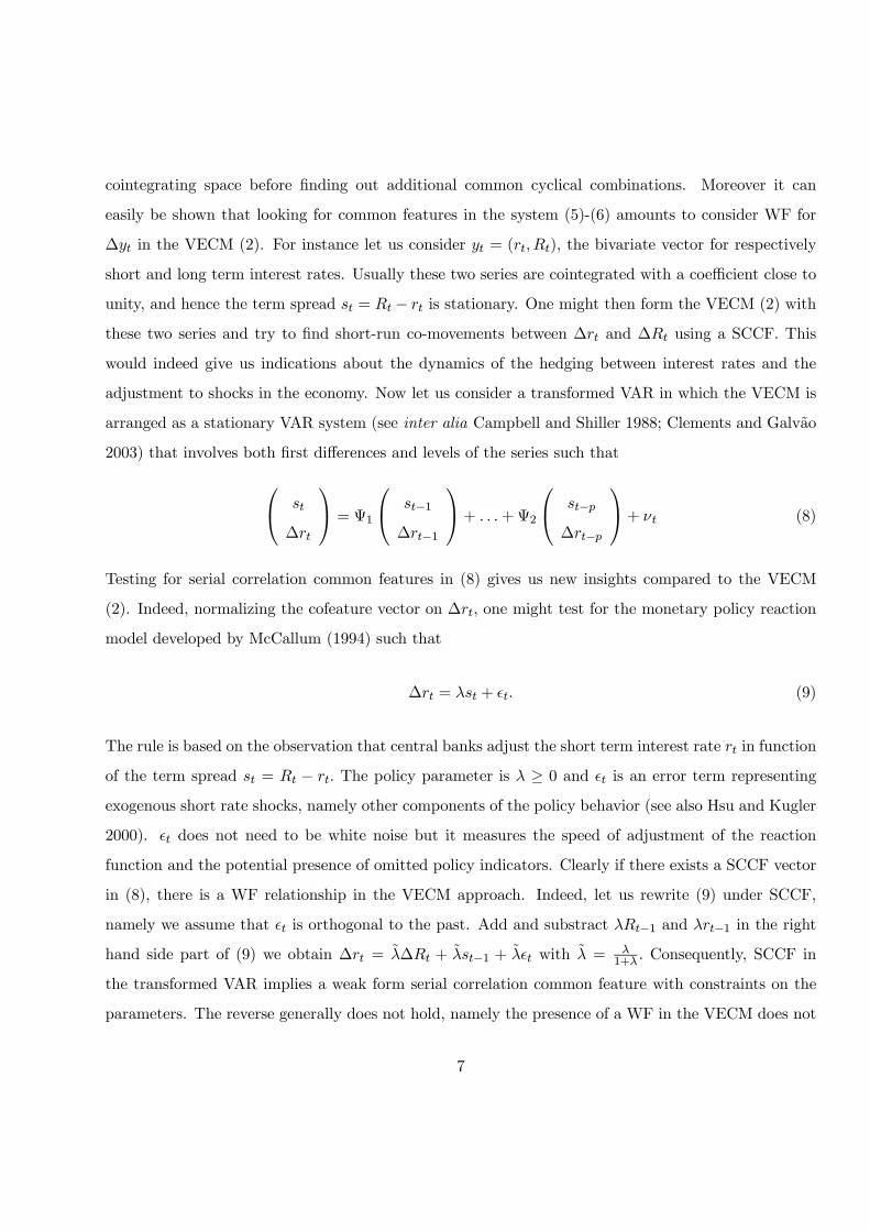
cointegrating space before finding out additional common cyclical combinations. Moreover it can

easily be shown that looking for common features in the system (5)-(6) amounts to consider WF for

∆yt in the VECM (2). For instance let us consider yt = (rt, Rt), the bivariate vector for respectively

short and long term interest rates. Usually these two series are cointegrated with a coefficient close to

unity, and hence the term spread st = Rt − rt is stationary. One might then form the VECM (2) with

these two series and try to find short-run co-movements between ∆rt and ∆Rt using a SCCF. This

would indeed give us indications about the dynamics of the hedging between interest rates and the

adjustment to shocks in the economy. Now let us consider a transformed VAR in which the VECM is

arranged as a stationary VAR system (see inter alia Campbell and Shiller 1988; Clements and Galvao

2003) that involves both first differences and levels of the series such that

st

∆rt

= Ψ1

st−1

∆rt−1

+ . . .+Ψ2 st−p

∆rt−p

+ νt (8)

Testing for serial correlation common features in (8) gives us new insights compared to the VECM

(2). Indeed, normalizing the cofeature vector on ∆rt, one might test for the monetary policy reaction

model developed by McCallum (1994) such that

∆rt = λst + ²t. (9)

The rule is based on the observation that central banks adjust the short term interest rate rt in function

of the term spread st = Rt − rt. The policy parameter is λ ≥ 0 and ²t is an error term representing

exogenous short rate shocks, namely other components of the policy behavior (see also Hsu and Kugler

2000). ²t does not need to be white noise but it measures the speed of adjustment of the reaction

function and the potential presence of omitted policy indicators. Clearly if there exists a SCCF vector

in (8), there is a WF relationship in the VECM approach. Indeed, let us rewrite (9) under SCCF,

namely we assume that ²t is orthogonal to the past. Add and substract λRt−1 and λrt−1 in the right

hand side part of (9) we obtain ∆rt = λ∆Rt + λst−1 + λ²t with λ = λ1+λ . Consequently, SCCF in

the transformed VAR implies a weak form serial correlation common feature with constraints on the

parameters. The reverse generally does not hold, namely the presence of a WF in the VECM does not

7

imply a SCCF in the transformed VAR.

3 TEST STATISTICS

3.1 The two-step approach

As a shortcut, the expression CanCor∆yt, yt−1|(D0t,∆y0t−1, . . .∆y0t−p+1)0 summarizes the reducedrank regression procedure used in the Johansen approach. That means that one extracts the squared

canonical correlations between ∆yt and yt−1, both sets concentrated out the effect of deterministic

terms and lags of ∆yt. In order to test for the significance of the r largest eigenvalues, one can rely on

Johansen’s trace statistic (10) or on one of the modified version to account for small samples like in

(11).

LRr = −TnX

i=r+1

ln(1− λi), (10)

LRcorr = −(T − np)nX

i=r+1

ln(1− λi), (11)

where the eigenvalues 1 > λ1 > ... > λn > 0 are the solution of |λS11 − S10S−100 S01| = 0. Sij , i, j = 0, 1are the second moment matrices of the residual R0t and R1t obtained in the multivariate least squares

regressions from respectively ∆yt and yt−1 on (D0t,∆y0t−1, . . .∆y0t−p+1)0. Under the null, these statistics

follow a functional of Brownian motions and asymptotic critical values can be found inter alia in

Johansen (1995) or in Osterwald-Lenun (1992). Approximations of the asymptotic distribution have

been proposed by Doornik (1998).

Once β has been found in a first step and superconsistently estimated by β, we can implement

the common feature test statistics. We make again the distinction between the SCCF and the WF

8

specifications. These are respectively based on the following reduced rank regressions:

SCCF : CanCor∆yt, (∆y0t−1, . . .∆y0t−p+1, y0t−1β)0|Dt,

WF : CanCor∆yt, (∆y0t−1, . . .∆y0t−p+1)0|(D0t, y0t−1β)0.

Both procedures allow to obtain the squared canonical correlations, namely the eigenvalues λSCCFi or

λWFi used to test for rank reductions. Note that for the weak form common cycle analysis, an equivalent

way to find the eigenvalues is through CanCor(∆y0t, y0t−1β)0, (∆y0t−1, . . .∆y0t−p+1, y0t−1β)0|Dt. For theVECM of order p− 1, the significance of the s smallest eigenvalues is evaluated through the followinglikelihood ratios:

LRSCCFs = −TsXi=1

ln(1− λSCCFi ) ∼ χ2(v1), s = 1 . . . n− r, (12)

LRWFs = −T

sXi=1

ln(1− λWFi ) ∼ χ2(v2), s = 1 . . . n, (13)

with v2 = s×n(p− 1)− s× (n− s) for the WF and v1 = s× (n(p− 1)+ r)− s× (n− s) for the SCCF.We also investigate the behavior of a correction for small sample sizes a la Reinsel and Ahn (1992),

i.e. LRSCCF cors = T−n(p−1)−r

T LRSCCFs and LRWF cors = T−n(p−1)

T LRWFs for respectively the SCCF

and the WF. The difference is due to the fact that in the WF, one concentrates out the cointegrating

vectors that are considered as known. Also remark that T is the real number of observations after

the deduction of initial points in regressions containing lags. Alternatively, information criteria can be

used (see also Vahid and Issler 2002). For p fixed and r given we can obtain these information criteria

for different values of reduced rank n− s using

ICT (p, r, s) = − 2Tlog lik +

λTT× (# parameters)

where the penalty λT is respectively 2, ln lnT and lnT for Akaike’s Information Criterion (AIC),

Hannan-Quinn Criterion (HQ) and Schwarz’s Bayesian Criterion (SC). Note that − 2T times the log

9

likelihood is nothing else than the log of the determinant of the reduced rank residuals covariance

matrix under common feature restrictions. The number of parameters is obtained by subtracting the

number of restrictions common dynamics impose from n2× (p−1)+nr, that is to say the total numberof parameters in the VECM for given r and p.

3.2 Switching algorithms

Hansen and Johansen (1998, p.95) show how to jointly impose cointegration and SCCF restrictions.

To illustrate the approach, let us consider a cointegrated VAR with an intercept, one lag in its VECM

form (i.e. p = 2 in the VAR) and common factor restrictions similar to (3) such that

∆yt = µ+ δ⊥Ψ01β0yt−1 + δ⊥Ψ02∆yt−1 + εt, (14)

where δ⊥ is the orthogonal complement of the cofeature matrix, namely δ0⊥δ = 0s×n and rank[δ : δ⊥] =

n. Hansen and Johansen (1998) impose SCCF restrictions by premultiplying (14) by the partitioning

matrix B,

B =

(δ0⊥δ⊥)−1δ0⊥| z

(n−s)×n

δ0|zs×n

to obtain

(δ0⊥δ⊥)−1δ0⊥∆yt = µ∗ +Ψ01β

0yt−1 +Ψ02∆yt−1 + (δ0⊥δ⊥)

−1δ0⊥εt, (15)

δ0∆yt = µ∗∗ + δ0εt, (16)

10

where µ∗ = (δ0⊥δ⊥)−1δ0⊥µ and µ∗∗ = δ0µ are vector column of size respectively (n − s) and s. Solving

(15) and (16) gives

(δ0⊥δ⊥)−1δ0⊥∆yt = (µ∗ − ωµ∗∗) +Ψ01β

0yt−1

+Ψ02∆yt−1 + ωδ0∆yt + (δ0⊥δ⊥)−1δ0⊥εt − ωδ0εt, (17)

where ω = Cov((δ0⊥δ⊥)−1δ0⊥εt, δ

0εt)V ar(δ0εt)−1.

Now, one finds that to obtain the cointegrating vectors under common feature restrictions we

consider CanCor(δ0⊥δ⊥)−1δ0⊥∆yt, yt−1|(1,∆y0t−1,∆y0tδ)0. The algorithm is as follows: (i) estimate β

without constraints in a first step, i.e. the usual Johansen approach; (ii) fixing the matrix β to its

estimated value, estimate s and δ; (iii) obtain the n− s common dynamic factors Ψ0 = (Ψ01,Ψ02) usingthe duality principle of canonical correlations; (iv) estimate δ⊥ in (14) by multivariate least squares.

Alternatively the orthogonal complement of δ can directly be obtained by standard routines such as

the command Null in GAUSS. This would merge steps (ii) to (iv). However this latter approach

is more sensitive to identifying restrictions on δ (see Gonzalo and Ng 2002); (v) reestimate β and

keep on iterating until convergence is reached. As pointed out by Hansen and Johansen (1998, p.97),

”there is no proof of convergence, but it will probably occur in practice, since each step maximized the

likelihood function for fixed values of the other parameters.” In the WF case there are not cross-equation

restrictions similar to (14), so the constrained model is simply

∆yt = µ+ αβ0yt−1 + δ⊥Ψ02∆yt−1 + εt. (18)

Imposing WF restrictions is convenient because this allows to consider both cointegration and common

feature test statistics without the constraint r + s ≤ n. To solve (18), we start by estimating β by

ML and we fix it to find the number of common feature vectors s. We estimate the n − s dynamiccommon factors forming Ψ02 in (18) and we use this constraint to reestimate β using the program

CanCor∆yt, yt−1|(1,∆y0t−1Ψ2)0. This sequence is iterated until convergence is reached. In our simu-lations, convergence is defined when the difference in the value of log-likelihood between two iterations

is less then 10−6. In both cases (SCCF and WF), tests for common features and cointegration can be

11

obtained by evaluating log-likelihood functions at their maxima for each models with r = 0 . . . n and

s = 0 . . . n and to form usual likelihood ratio tests by taking twice their differences.

4 MONTE CARLO EXERCISE

4.1 The data generating process

The underlying data generating process is a stylized second order VAR with four I(1) variables and

two cointegrating vectors:

∆y1t

∆y2t

∆y3t

∆y4t

=

.25

−.15−.1.5

+−.2 .2

−.8 −.4−1 .8

−.5 0

1 0 1.2 −10 1 −.8 −1

y1t−1

y2t−1

y3t−1

y4t−1

+

−.1−.4−.2−.25

³2 1 1 1

´∆y1t−1

∆y2t−1

∆y3t−1

∆y4t−1

+

ε1t

ε2t

ε3t

ε4t

. (19)

In (19) there also exist three weak form common feature vectors, i.e. rank(Γ1) = 1. These three

normalized linearly independent cofeature vectors are δ01 = (1 − .25 0 0) , δ02 = (1 0 − .5 0) and δ03 =

(1 0 0 − .4) . It is shown in Hecq, Palm and Urbain (2005) that sWF vectors imply s−r SCCF vectors.This is a direct extension of Vahid and Engle (1993)’s lemma which shows that in a cointegrated

VAR(1), i.e. a model with n WF vectors, there exist n − r SCCF vectors. In this case there existsone SCCF vector. But this vector suffers from identification problems. In this example, the roots of

the determinant of the characteristic equation are 1, 1, -1.55, 1.02±.35i. Disturbances εit follow a zeromean Gaussian distribution with variances 1 and all covariances equal 0.7. Three sample sizes are

considered: T = 50, 100, 200. Computations have been carried out using GAUSS; 10,000 replications

are used; the first 50 observations are discarded to remove dependence on initial observations.

Next we present in two distinct subsections outcomes for cointegration and for common features.

12

4.2 Results on cointegration

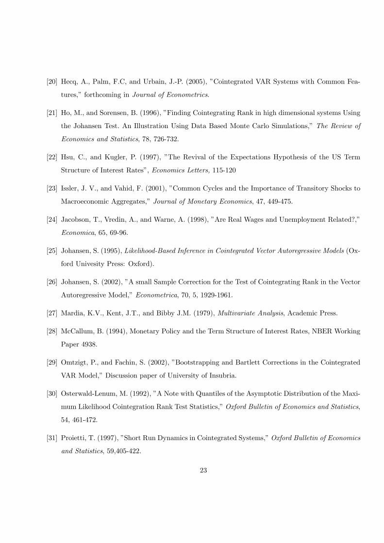
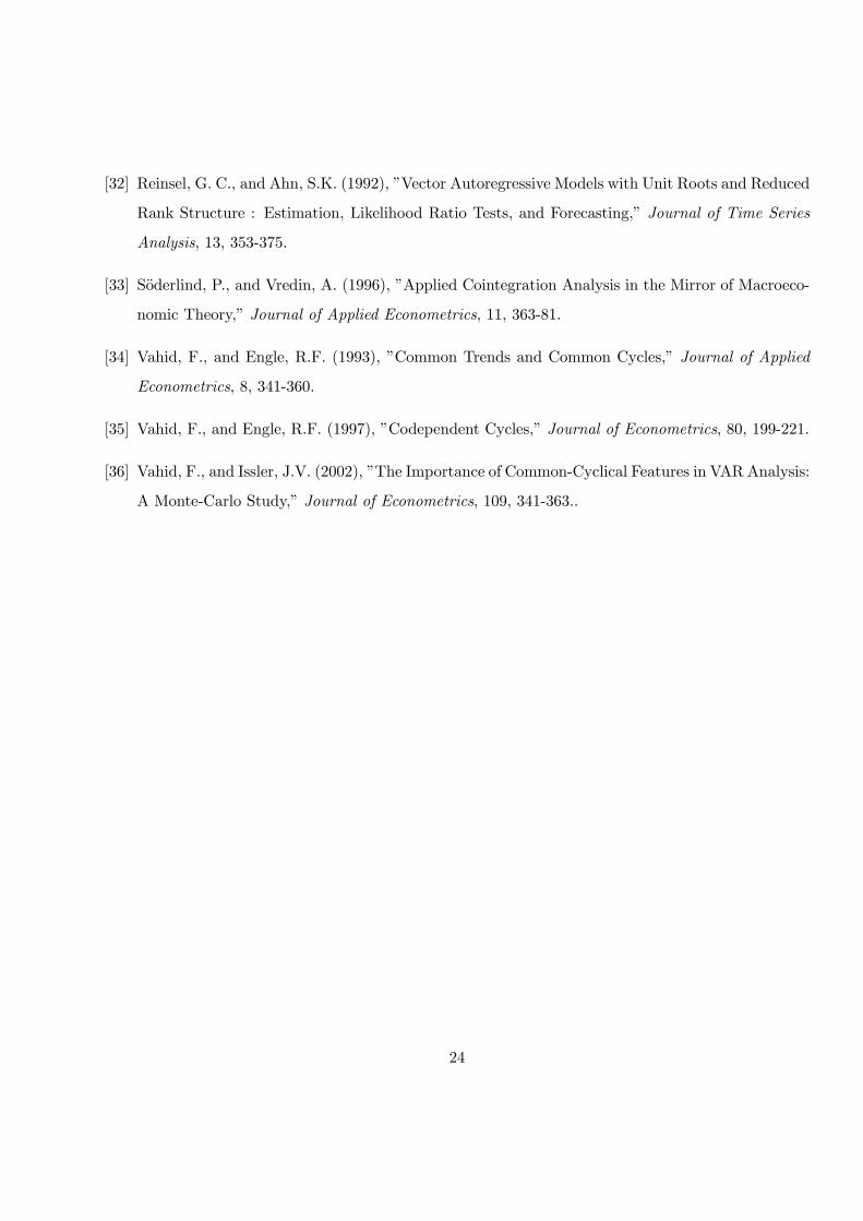
Tables 1 and 2 report empirical sizes and size unadjusted powers of Johansen’s trace statistics (model

with an unconstrained constant) when imposing WF common feature restrictions. The nominal size

is 5% with asymptotic critical values given in Osterwald-Lenun (1992). Rows labelled s = 0 report

the rejection frequencies when no common feature restrictions are imposed. For s = 1, 2, 3, 4 we report

rejection frequencies obtained using the ”zigzag” procedure to reach the maximum. s = 3 is the

correct number of restrictions. When one overestimates s, i.e. s = 4, the estimated system reduces to

a VAR(1). We consider in Table 1 the case of a correct choice of the lag length, i.e. p = 2. Table 2

proposes the same output when we take p = 4 and thus we overestimate the lag order in the estimated

model. Both tables give the rejection frequencies of the asymptotic trace test (10) and its small sample

corrected version (11).

There are two cointegrating vectors in the DGP. Consequently, rejection frequencies under the

hypotheses r = 0 and r ≤ 1 measure the unadjusted empirical power, that is to say the probability toreject respectively zero and one cointegrating vector for a higher number. A relatively small rejection

frequency in these columns indicates that we might consider too few long-run relationships. For the

size properties we focus on the column H0 : r ≤ 2 whose values should be in the vicinity of 5%, thenominal size. A higher rejection frequency emphasizes the detection of too many cointegrating vectors.

The last column H0 : r ≤ 3 gives the likelihood to obtain a system with n stationary variables.

================================

INSERT TABLEs 1 & 2 ABOUT HERE

================================

Some comments are in order:

• For s = 0, namely the case without short-run restrictions, we observe size distortions for small

samples (with T = 50 and to a lesser extent with T = 100). Empirical sizes based on asymptotic

tests are about 16% for T=50 and 9% for T=100 whatever the choice of p. The small sample

correction behaves quite well when p = 2 but improperly when p increases: the strong correction

13

by T − np leads to underestimating the number of cointegrating vectors (empirical size less than5%).

• s = 4 means we end up with a VAR(1) and consequently the dynamics are underestimated. Thiscreates size distortions.

We have already mentioned that these issues are well documented in the literature. Next we consider

the effect of also imposing common feature restrictions. In these cases (rows s = 1, 2, 3) we observe

that:

• Taking into account the common feature restrictions always slightly reduces (mainly for T=50)size distortions, the reduction being at its maximum with the correct number of restrictions, i.e.

s = 3. The difference is not so huge however. For instance with p = 4 and 50 observations, the

asymptotic test statistics (10) has an empirical size of 16.98% while the size with s = 3 is 13.33%.

• The switching approach also helps in not rejecting the null that r ≤ 3 and thus to find a fourthcointegrating vector. This will be illustrated in the empirical section where, based on asymptotic

distributions, we first find six cointegrating vectors among six countries.

• Another interesting aspect when testing for cointegration under WF restrictions is also the in-crease in power when the lag length is large. With T = 50 and for s = 0, we determine in only

10% the presence of at least a second cointegrating vector for the small sample corrected statistics

while this proportion increases to 63% with s = 3. Similar results are observed for r = 0. The

power of the test being only 53% in the usual approach but reaches 100% if we use the ”zigzag”

one.

As expected, we see that in VAR with longer lags, common feature restrictions are helpful to

improve the performance of both the power and the size of cointegration test statistics. In practice,

the biggest empirical problem could be to know whether we face a power problem (asymptotic tests

cannot detect the whole set of long-run relationships) or a size one (tests detect too many). Next we

evaluate the impact of the switching procedure on common feature test statistics.

14

4.3 Results on common features

Tables 3 and 4 present for respectively p = 2 and p = 4 in the estimated VAR models, different testing

strategies to find out WF common features. On the one hand there are the two-step approach and

likelihood ratios based on the iterative estimation, both using the asymptotic test and the modified

version. We only stress the size properties, namely the frequency to reject the null hypothesis there

exists three common feature vectors, i.e. s = 3. The results about the empirical power, i.e. the rejection

of the existence of a fourth common feature vector is rejected in 100% of the cases and is not reported.

On the other hand we also present the percentage of finding s = 3 using information criteria. In the

tables, we only report in the tables the frequencies to correctly find s = 3 within the 2-step approach.

We comment on results obtained via the switching framework in the text.

===============================

INSERT TABLES 3 & 4 ABOUT HERE

===============================

These tables report the results when choosing different cointegrating vectors r = 1 to 3.With r = 4,

it does not make sense to ”zigzag” because the cointegrating space spans IRn. In all these cases the

cointegrating vectors are estimated. In order to have a benchmark, we also show the results with r = 2

but with the coefficients of β fixed to their true values (entry βr=2 instead of βr=2).

The following results emerge:

• As it is noticed in Hecq, Palm and Urbain (2005) the performance of test statistics is dramaticallyaltered when r is underestimated, i.e. the rows with r = 1. This is the reason why it is sensible to

first fix the cointegrating rank to its upper plausible bound. For instance, to start with r = n−1in a convergence analysis.

• Comparing the columns where respectively the 2-step and the iterative procedure are reportedwe observe that when p is large, the switching procedure reduces the size distortions. This is less

visible with p = 2 because there is only a small difference between imposing and not imposing

the restrictions.

15

• One should recognize the relatively good performance of these test given the underlying largenumber of restrictions: respectively 9 and 33 for p = 2 and p = 4. In particular, small sample

corrections seem to work well. For instance, with r = 2, p = 4 and T = 50 , the empirical

size is 9.7% with the small sample correction and 45.82% without it. Notice that for the same

specification, a two steps strategy would respectively yield empirical sizes of 20.82% and 57.85%.

For 100 observations the sizes are quite close to the nominal ones.

• However, for small T these size distortions are still larger than the ones obtained with known

cointegrating vectors.

• Information criteria work remarkably well and especially the SC (frequency to find s = 3 is alwayshigher than 95%) and to a lesser extent the HQ. What is generally not appreciated in practice

with the SC, that is to say, the fact that it is often too parsimonious when considering the lag

length of a VAR for instance, seems to be an advantage here.

• The AIC has the tendency to pick up too few common feature vectors. This is a bit better whenthe cointegrating vectors are known. In order to point out the influence of the estimation of β,

we have also computed these information criteria in the iterative approach. For instance, with

T = 50 the frequency to correctly find s = 3 for the AIC, HQ and SC are 69.07%, 88.16% and

97.86% for p = 2 and 54.40%, 89.13%, 99.53% for p = 4. This is higher than the numbers from

Tables 3 and 4, especially for AIC and HQ.

Overall, we first might say that for the cofeature analysis the iterative procedure may help if

combined with an adjustment for small samples. The issue of this paper was not to compare the

merits of different small sample versions for common feature test statistics. At least we have illustrated

that anything is better than to rely on asymptotic distributions. For instance, instead of using the

small sample correction a la Reinsel and Ahn we could have considered a Bartlett correction (see

Mardia, Kent and Bibby, 1979) by replacing respectively (T − n(p − 1)) and (T − n(p − 1) − r) by(T − 1

2(n + n(p − 1) + 3)) and (T − 12(n + n(p − 1) + r + 3)). For the DGP (19), these Bartlett’s

style modified statistics behave better for p = 2, are equivalent to the one proposed in this paper for

p = 3 and the correction a la Reinsel and Ahn is far better when p = 4. Secondly, we must be careful

16

and avoid underestimating the number of cointegrating vectors. Thirdly, information criteria and in

particular the SC are tools we should not forget.

We do not report the results of the SCCF test statistics since we want to let r and s vary freely.

The underlying DGP (19) implies one SCCF vector but to detect it, it is better to rely on the mixed

form framework developed in Hecq, Palm and Urbain (2005). To simplify the analysis, we consider

the same DGP but with Γ1 = 0n×n. In this case, we have a VAR(1) and the space spanned by δ is

actually the space spanned by the columns of α⊥. We consider the case with T = 50 and p = 2 in the

estimated model and compare the SCCF empirical sizes (H0 : s = 2) when β is known or estimated.

In the latter case we can analyze the effect of an overestimation of the number of cointegrating vector

r. The following pairs refer to the asymptotic and the modified tests respectively. When β is fixed to

its true value we obtain the rejection frequencies (9.65% , 5.22%). When β is estimated, the two step-

approach gives respectively (14.63% , 8.83%) and (47.43% , 30.09%) for r = 2 and r = 3. A switching

procedure reduces these percentages. But the important point here is the large size distortion when

overestimating r. This explains why we have proposed to start with the WF to determine r and s and

then to look at SCCF for some plausible number of common feature vectors. This approach is applied

in the next section.

5 COMMON CYCLES-COMMON TRENDS IN LATIN AMER-

ICA

This section investigates the presence of short and the long-run interactions between the output of six

Latin American economies: Brazil, Venezuela, Mexico, Peru, Columbia and Chile. We consider two

datasets, one for the real gross domestic product (RGDP hereafter) and another one with output per

capita series (RGDP K hereafter). The annual variables span the period 1950-2002, thus a sample of 53

observations for n = 6. The source is: Groningen Growth and Development Centre and The Conference

Board, Total Economy Database, release August 2004 (see http://www.ggdc.net). A ”pretest” check

pleaded for excluding Argentina from the study. Indeed, adding Argentina made the analysis less

robust for the identification of the VAR order and the number of cointegrating vectors. Moreover it

was quite difficult to fit a system in which Argentinian variables were significant.

17

We consider the model with a restricted deterministic trend in the long-run and five lags were

necessary to capture the dynamics of the multivariate process. Table 5 reports Johansen’s trace test.

Familiar results emerge: the asymptotic test probably overestimates the number of cointegrating vectors

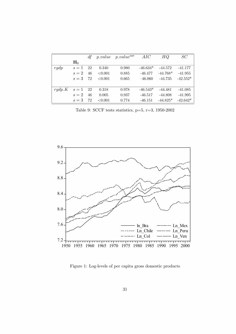
as we reject the null H0 : r ≤ 5. As it is illustrated in Figure 1 for per capita series, it is indeed quiteunlikely that all output variables are stationary around a deterministic trend. Similarly the short-run

correction penalizes too much. Probably r should lie between two and five for these two samples. The

determination of the number of long-run relationships however is crucial for the interpretation of the

convergence among economies (see inter alia Bernard and Durlauf 1995).

=======================================

INSERT TABLE 5 and FIGURE 1 ABOUT HERE

=======================================

We leave the determination of the cointegrating rank unsolved for the moment and we go ahead

with the analysis of short-run co-movements. We have seen that an overestimation of r only marginally

affects the weak form common cycle test statistic while underestimating r gives misleading answers.

Consequently we choose r = 5 for a 2-step approach presented in Table 6. We report the value of

the asymptotic likelihood ratio test (10), its associated degrees of freedom, the p − values for boththe asymptotic and the small sample corrected version (11) and the three information criteria. The

observations made in the Monte Carlo experiment are again well illustrated here and are quite helpful to

understand the results. Indeed, asymptotic tests would favor s = 0, namely no common feature vectors,

while we would choose s = 2 for the real output series and maybe s = 3 for the per capita real output

based on small sample modified versions. AIC would take s = 0 or s = 1, HQ s = 1 but SC would

favor s = 3 for both sets of variables. Also note that the iterative approach only marginally changes

the results and consequently these outcomes are not reported to save space. Indeed, with r = 5 there

are only few additional restrictions. We have noticed (results not reported) that the biggest difference

is in the first panel (i.e. RGDP) where the p− value for not rejecting a third common feature vectoris 0.05 instead of 0.03. The information criteria give the same conclusions.

18

=============================

INSERT TABLE 6 ABOUT HERE

=============================

We continue the analysis and we purposely consider the three possibilities offered by cofeature

tests in Table 6, namely s = 1, 2 or 3. For each s we then test for cointegration using the iterative

approach. From Table 7 we would recommend r = 3. The reason is that it emerged from Table 6

that there probably exist three common feature vectors and in the column s = 3 the values of the

asymptotic tests are quite different between rejecting the null hypothesis of less than two and less then

three cointegrating vectors. For r = 3, Table 8 reports the results for the common feature switching

approach. P − values for asymptotic and small sample corrected tests are presented together with thevalues of iterated information criteria. Now there is a clear cut in favor of s = 3 if we look at the

corrected test and either the HQ and the SC.

We have an interesting result here because there are as many long-run co-movements as short-run

ones or say differently, there exist three permanent and three transitory shocks driving the output of

the six countries. Moreover, the constraint s + r ≤ n allows us to go further and to analyze whetherthe three weak form cofeature relationships are also SCCF vectors (see Hecq, Palm and Urbain 2005).

We use the algorithm exposed in Section 3.2., that is to say we fix r = 3 and we test for the number of

SCCF vectors by iterating between the cointegrating and the common feature spaces. Table 9 reveals

that we cannot reject the null of three serial correlation common feature vectors if we look at small

sample corrected likelihood ratio tests, or more exactly the p− values associated with these tests. SCalso favors s = 3 while HQ takes s = 3 for per capita series and s = 2 for the other dataset. AIC

and asymptotic likelihood ratio tests would keep s = 1 but we are aware from the Monte Carlo results

that these two latter procedures might underestimate the number of common feature vectors in small

samples. This result also means that by definition the three WF vectors were also SCCF ones. To

formally study this issue we can compare the Schwarz criteria obtained in Tables 8 and 9 for s = 3. It

emerges that their values are smaller for both datasets for SCCF than for WF.

This case with r + s = n is ideal for extracting the long and the short-run co-movements because

these components are exactly identified. Simple methods might be considered such as the one proposed

19

in Vahid and Engle (1993) for the Beveridge-Nelson cycles. This latter decomposition would be identical

to the Gonzalo-Granger (1995) ones were the three common cycles are given by β0yt and the common

trends by δ0yt. Namely we only need estimated cointegrating and common feature vectors that maximize

the likelihood after the convergence of iterations has been reached. We do not graph these components

because the scope was to point out that misleading results concerning the number of co-movements can

be obtained when working with small samples. Moreover we do not want to give the false impression

commonly shared in the literature that finding r+ s = n is the final goal of a common trend - common

cycle study.

===================================

INSERT TABLES 7, 8 & 9 ABOUT HERE

===================================

6 CONCLUSION

In this paper, we studied a linear Gaussian VAR model with non-stationary but cointegrated variables

that have common cyclical features. Similarly to other papers we have pointed out through Monte Carlo

simulations that cointegrating test statistics but also common feature procedures based on asymptotic

distributions suffer from size distortions. Iterating or ”zigzagging”, as we called it, between spaces helps

to reduce the size distortion observed in Johansen’s trace test but without reaching the nominal size.

However the power is improved. Common feature test statistics behave quite well and especially if we

combine a switching approach with a small sample correction. Information criteria work remarkably

well, in particular the Schwarz’s criterion that had already a good behavior in a 2-step approach which

can be improved by iterating between cointegrating and common feature spaces. Consequently, we

propose another strategy than the one advocated in Vahid and Issler (2002). Indeed for forecasting

purposes they show that the best strategy is to let p and s (SCCF vectors) be ”freely” chosen by

information criteria and in particular by the HQ. In our case, for determining the number of long

and short-run co-movements we propose to choose the lag order in the VAR with AIC for instance

(Gonzalo and Pitarakis 2002) and then to test for cointegration. One can choose a maximum r and

20

test for WF common features using small sample likelihood ratio tests and information criteria (SC).

In summary, different information criteria are best used for different purposes. Having determined r

and s WF vectors, the presence of SCCF relationships can be tested for r + s ≤ n. This strategy

helps us to determine the existence of three permanent and three transitory shocks within the six Latin

American economies whatever the dataset we use. If we had blindly trust the asymptotics, we would

have obtained that six transitory shocks drive the economies!

References

[1] Anderson, T.W. (1984), An Introduction to Multivariate Statistical Analysis, 2nd Ed. (John Wiley

& Sons).

[2] Beine, M., and Hecq A. (1999), ”Inference in Codependence : Some Monte Carlo Results and

Applications, ” Annales d’Economie et de Statistique, 54, 69-90.

[3] Bernard, A.B., and Durlauf, S.N. (1995), ”Convergence in International Output,” Journal of

Applied Econometrics, 10, 97-108.

[4] Campbell, J.Y., and Shiller, R.J. (1988), ”The Dividend-Price Ration and Expectations of Future

Dividends and Discount Factors”, The Review of Financial Studies, vol. 1, 3, 195-228.

[5] Candelon, B, Hecq A., and Verschoor, W. (2005), ”Measuring Common Cyclical Features During

Financial Turmoil,” forthcoming in Journal of International Money and Finance.

[6] Cheung Y.-W., and Lai, K.S. (1993), ”Finite-sample Sizes of Johansen’s Likelihood Ratio Tests

for Cointegration,” Oxford Bulletin of Economics and Statistics, 55, 313-28.

[7] Clements, M.P., and Galvao, A.B. (2003), ”Testing the Expectations Theory of the Term Structure

of Interest Rates in Threshold Models”, Macroeconomic Dynamics, 7, 567-85.

[8] Cubadda, G., and Hecq, A. (2001), ”On Non-contemporaneous Short-Run Comovements,” Eco-

nomics Letters, 73, 389-397.

21

[9] Doornik, J. A. (1998), ”Approximations to the asymptotic distribution of cointegration tests,”

Journal of Economic Surveys, 12, 573—593.

[10] Engle, R. F., and Kozicki, S. (1993), ”Testing for Common Features (with comments),” Journal

of Business and Economic Statistics, 11, 369-395.

[11] Fachin, S. (2000), ”Bootstrap and Asymptotic Tests of Long-run Relationships in Cointegrated

Systems,” Oxford Bulletin of Economics and Statistics, 62, 511-532.

[12] Gonzalo, J., and Granger, C.W.J. (1995), ”Estimation of Common Long-Memory Components in

Cointegrated Systems,” Journal of Business and Economics Statistics, 33, 27-35

[13] Gonzalo, J., and Pitarakis, J.Y. (1999), ”Dimensionality Effect in Cointegration Analysis,” Chap-

ter 9 in Engle R. and H. White (Ed.), Cointegration, Causality, and Forecasting. A Festschrift in

Honour of Clive W.J Granger, (Oxford University Press).

[14] Gonzalo, J., and Ng, S. (2001), ”A Systematic Framework for Analyzing the Dynamic Effects of

Permanent and Transitory Shocks,” Journal of Economic Dynamics & Control, 25, 1527-1546.

[15] Gonzalo, J., and Pitarakis, J.Y. (2002), ”Lag Length Estimation in Large Dimensional Systems,”

Journal of Time Series Analysis.

[16] Hansen, P.R. and Johansen, S. (1998), Workbook on Cointegration, (Oxford University Press:

Oxford).

[17] Harris, R.I.D. and Judge, G. (1998), ”Small Sample Testing for Cointegration using the Bootstrap

Approach,” Economics Letters, 58, 31-37.

[18] Hecq, A.(1998), ”Does Seasonal Adjustment Induce Common Cycles?,” Economics Letters, 59,

289-297.

[19] Hecq, A., Palm, F.C, and Urbain, J.-P. (2000), ”Permanent-Transitory Decomposition in VAR

Models with Cointegration and Common Cycles,” Oxford Bulletin of Economics and Statistics,

62, 543-552.

22

[20] Hecq, A., Palm, F.C, and Urbain, J.-P. (2005), ”Cointegrated VAR Systems with Common Fea-

tures,” forthcoming in Journal of Econometrics.

[21] Ho, M., and Sorensen, B. (1996), ”Finding Cointegrating Rank in high dimensional systems Using

the Johansen Test. An Illustration Using Data Based Monte Carlo Simulations,” The Review of

Economics and Statistics, 78, 726-732.

[22] Hsu, C., and Kugler, P. (1997), ”The Revival of the Expectations Hypothesis of the US Term

Structure of Interest Rates”, Economics Letters, 115-120

[23] Issler, J. V., and Vahid, F. (2001), ”Common Cycles and the Importance of Transitory Shocks to

Macroeconomic Aggregates,” Journal of Monetary Economics, 47, 449-475.

[24] Jacobson, T., Vredin, A., and Warne, A. (1998), ”Are Real Wages and Unemployment Related?,”

Economica, 65, 69-96.

[25] Johansen, S. (1995), Likelihood-Based Inference in Cointegrated Vector Autoregressive Models (Ox-

ford Univesity Press: Oxford).

[26] Johansen, S. (2002), ”A small Sample Correction for the Test of Cointegrating Rank in the Vector

Autoregressive Model,” Econometrica, 70, 5, 1929-1961.

[27] Mardia, K.V., Kent, J.T., and Bibby J.M. (1979), Multivariate Analysis, Academic Press.

[28] McCallum, B. (1994), Monetary Policy and the Term Structure of Interest Rates, NBER Working

Paper 4938.

[29] Omtzigt, P., and Fachin, S. (2002), ”Bootstrapping and Bartlett Corrections in the Cointegrated

VAR Model,” Discussion paper of University of Insubria.

[30] Osterwald-Lenum, M. (1992), ”A Note with Quantiles of the Asymptotic Distribution of the Maxi-

mum Likelihood Cointegration Rank Test Statistics,” Oxford Bulletin of Economics and Statistics,

54, 461-472.

[31] Proietti, T. (1997), ”Short Run Dynamics in Cointegrated Systems,” Oxford Bulletin of Economics

and Statistics, 59,405-422.

23

[32] Reinsel, G. C., and Ahn, S.K. (1992), ”Vector Autoregressive Models with Unit Roots and Reduced

Rank Structure : Estimation, Likelihood Ratio Tests, and Forecasting,” Journal of Time Series

Analysis, 13, 353-375.

[33] Soderlind, P., and Vredin, A. (1996), ”Applied Cointegration Analysis in the Mirror of Macroeco-

nomic Theory,” Journal of Applied Econometrics, 11, 363-81.

[34] Vahid, F., and Engle, R.F. (1993), ”Common Trends and Common Cycles,” Journal of Applied

Econometrics, 8, 341-360.

[35] Vahid, F., and Engle, R.F. (1997), ”Codependent Cycles,” Journal of Econometrics, 80, 199-221.

[36] Vahid, F., and Issler, J.V. (2002), ”The Importance of Common-Cyclical Features in VAR Analysis:

A Monte-Carlo Study,” Journal of Econometrics, 109, 341-363..

24

H0 : r = 0 r ≤ 1 r ≤ 2 r ≤ 3

T s LRr LRcorr LRr LRcorr LRr LRcorr LRr LRcorr50 s = 0 100 100 99.54 96.33 15.41 7.08 7.03 4.74

s = 1 100 100 99.58 96.52 15.32 7.16 6.97 4.60

s = 2 100 100 99.63 97.46 14.94 7.05 6.78 4.36

s = 3 100 100 100 100 13.10 6.04 5.78 3.59

s = 4 100 100 79.59 67.62 44.75 31.16 13.91 9.96

100 s = 0 100 100 100 100 8.35 5.86 4.48 3.42

s = 1 100 100 100 100 8.30 5.89 4.44 3.45

s = 2 100 100 100 100 8.25 5.63 4.46 3.47

s = 3 100 100 100 100 7.89 5.28 4.08 3.03

s = 4 100 100 97.39 95.46 64.91 59.86 13.37 11.38

200 s = 0 100 100 100 100 6.26 4.96 2.74 2.35

s = 1 100 100 100 100 6.3 4.92 2.72 2.34

s = 2 100 100 100 100 6.17 4.89 2.74 2.34

s = 3 100 100 100 100 5.89 4.62 2.72 2.35

s = 4 100 100 100 100 71.63 69.31 12.44 11.41

Table 1: Rejection frequencies of Johansen’s trace test - Switching procedure with WF restrictions anda lag length p=2 in the estimated model

25

H0 : r = 0 r ≤ 1 r ≤ 2 r ≤ 3

T s LRr LRcorr LRr LRcorr LRr LRcorr LRr LRcorr50 s = 0 98.45 53.03 68.16 10.07 16.98 1.52 10.49 3.83

s = 1 98.99 60.14 71.74 12.52 16.53 1.82 9.15 3.26

s = 2 99.84 82.98 81.13 23.63 15.23 2.45 7.66 2.50

s = 3 100 100 96.54 63.27 13.33 1.69 5.92 1.88

s = 4 100 100 79.59 50.32 44.75 16.55 13.91 5.85

100 s = 0 100 100 97.01 84.79 9.66 4.25 5.97 3.55

s = 1 100 100 97.94 87.72 9.66 4.19 5.61 3.38

s = 2 100 100 98.80 93.16 8.87 3.81 5.06 3.10

s = 3 100 100 100 99.98 7.89 3.29 4.06 2.36

s = 4 100 100 97.39 92.13 64.91 53.52 13.27 9.29

200 s = 0 100 100 100 100 6.67 4.10 3.03 2.23

s = 1 100 100 100 100 6.40 4.07 3.03 2.29

s = 2 100 100 100 100 6.30 3.84 2.75 2.20

s = 3 100 100 100 100 5.78 3.76 2.68 2.02

s = 4 100 100 100 100 71.63 66.97 12.44 10.76

Table 2: Rejection frequencies of Johansen’s trace test - Switching procedure with WF restrictions anda lag length p=4 in the estimated model

26

H0 : s = 3 2-step Iterative 2-step

LRs LRcors LRs LRcors AIC HQ SC

T = 50 βr=1 99.79 99.67 98.36 97.95 0.10 0.32 0.83

βr=2 18.06 13.77 15.03 10.84 64.85 85.50 97.05

βr=3 17.61 12.87 16.38 11.83 65.41 85.94 97.50

βr=4 16.91 12.15 − 66.31 86.55 97.62

βr=2 11.69 8.3 − 73.85 90.64 98.71

T = 100 βr=1 100 100 99.98 99.96 0 0 0.01

βr=2 9.92 8.24 9.08 7.37 76.24 95.21 99.71

βr=3 9.96 8.17 9.49 7.68 76.08 95.16 99.74

βr=4 9.64 7.90 − 76.53 95.36 99.74

βr=2 7.78 6.37 − 79.11 96.62 99.82

T = 200 βr=1 100 100 100 100 0 0 0

βr=2 7.19 6.61 6.92 6.28 80.57 98.02 99.99

βr=3 7.45 6.7 7.30 6.52 80.33 98.03 99.98

βr=4 7.27 6.55 − 80.31 98.08 99.98

βr=2 6.58 5.95 − 81.85 98.21 99.99

Table 3: Empirical size of the 2-step and the iterative WF common feature tests and informationcriteria, p=2 in the estimated model

27

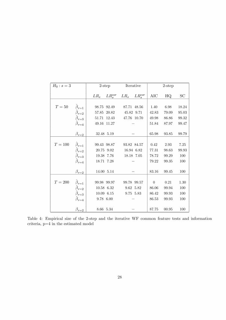
H0 : s = 3 2-step Iterative 2-step

LRs LRcors LRs LRcors AIC HQ SC

T = 50 βr=1 98.75 92.49 87.71 48.56 1.40 6.98 18.24

βr=2 57.85 20.82 45.82 9.71 42.83 79.09 95.03

βr=3 51.71 12.43 47.76 10.70 49.98 86.86 99.32

βr=4 49.16 11.27 − 51.84 87.97 99.47

βr=2 32.48 5.19 − 65.98 93.85 99.79

T = 100 βr=1 99.43 98.87 93.82 84.57 0.42 2.93 7.25

βr=2 20.75 9.02 16.94 6.82 77.31 98.63 99.93

βr=3 19.38 7.76 18.18 7.05 78.72 99.29 100

βr=4 18.71 7.28 − 79.22 99.35 100

βr=2 14.00 5.14 − 83.16 99.45 100

T = 200 βr=1 99.98 99.97 99.78 99.57 0 0.21 1.30

βr=2 10.58 6.32 9.62 5.82 86.06 99.94 100

βr=3 10.09 6.15 9.75 5.83 86.42 99.93 100

βr=4 9.78 6.00 − 86.53 99.93 100

βr=2 8.66 5.34 − 87.75 00.95 100

Table 4: Empirical size of the 2-step and the iterative WF common feature tests and informationcriteria, p=4 in the estimated model

28

H0 λi LRr LRcorr 95%cv

rgdp K r = 0 0.936 370.95 * 139.10 * 114.96r ≤ 1 0.837 238.63 * 89.48 * 86.96r ≤ 2 0.723 151.29 * 56.73 62.61r ≤ 3 0.581 89.62 * 33.60 42.20r ≤ 4 0.414 47.81 * 17.93 25.47r ≤ 5 0.369 22.12 * 8.29 12.39

rgdp r = 0 0.939 371.72 * 139.39 * 114.96r ≤ 1 0.824 237.39 * 89.02 * 86.96r ≤ 2 0.725 153.82 * 57.68 62.61r ≤ 3 0.603 91.71 * 34.39 42.20r ≤ 4 0.437 47.35 * 17.75 25.47r ≤ 5 0.336 19.72 * 7.39 12.39

Table 5: Cointegration trace statistics for the six Latin American economies over 1950-2002 - Modelwith a restricted trend in the long-run, p=5

H0 LRWFs df p val p valcor AIC HQ SC

rgdp s = 0 − − − − -47.220* -44.657 -40.437

s = 1 39.91 19 0.003 0.397* -47.180 -44.897* -41.138

s = 2 103.58 40 <0.001 0.100* -46.729 -44.755 -41.505

s = 3 170.67 63 <0.001 0.030 —46.290 -44.654 -41.962*

s = 4 290.28 88 <0.001 0.001 -44.839 -43.572 -41.487

s = 5 423.44 115 <0.001 <0.001 -43.190 -42.321 -40.890

s = 6 584.79 144 <0.001 <0.001 -41.037 -40.596 -39.868

rgdp K s = 0 − − − − -47.044 -44.482 -40.261

s = 1 35.89 19 0.011 0.526* -47.088* -44.805* -41.046

s = 2 93.78 40 <0.001 0.210* -46.757 -44.783 -41.533

s = 3 161.93 63 <0.001 0.063* -46.296 -44.660 -41.968*

s = 4 282.11 88 <0.001 <0.001 -44.833 -43.566 -41.481

s = 5 412.28 115 <0.001 <0.001 -44.246 -42.377 -40.946

s = 6 565.80 144 <0.001 <0.001 -41.256 -40.814 -40.087

Table 6: 2-step WF common feature tests statistics with p=5 and r=5, 1950-2002

29

s = 1 s = 2 s = 3

H0 LRr LRcorr LRr LRcorr LRr LRcorrrgdp K r = 0 353.91* 132.71* 320.94* 120.35* 287.89* 107.96

r ≤ 1 226.90* 85.08 200.30* 75.11 166.35* 62.38

r ≤ 2 137.94* 51.72 116.57* 43.71 95.98* 35.99

r ≤ 3 73.28* 27.48 50.96* 19.11 33.73 12.62

r ≤ 4 30.98* 1.61 21.08 7.90 16.21 6.08

r ≤ 5 8.26 3.09 8.44 3.16 3.78 1.41

rgdp r = 0 350.12* 131.29* 314.77* 118.04* 296.28* 111.10

r ≤ 1 219.79* 82.42 191.57* 71.84 175.16* 65.68

r ≤ 2 136.21* 51.08 116.72* 43.76 101.90* 38.21

r ≤ 3 70.64* 26.49 51.46* 19.29 37.69 14.13

r ≤ 4 28.54* 10.70 20.80 7.80 13.64 5.11

r ≤ 5 8.10 3.04 6.12 2.29 6.23 2.33

Table 7: Iterative cointegration trace statistics, p=5, 1950-2002

LRs df p val p valcor AIC HQ SCH0

rgdp s = 1 19.03 19 0.454 0.963 -46.615* -44.509 -41.041

s = 2 64.96 40 0.007 0.795 -46.534 -44.736 -41.778

s = 3 124.97 63 <0.001 0.494 —46.242 -44.783* -42.382*

s = 4 234.92 88 <0.001 0.019 -44.993 -43.902 -42.108

s = 5 362.89 115 <0.001 <0.001 -43.452 -42.759 -41.619

rgdp K s = 1 19.12 19 0.449 0.962 -46.531 -44.425 -40.957

s = 2 59.57 40 0.023 0.881 -46.563* -44.766 -41.807

s = 3 121.69 63 <0.001 0.553 -46.228 -44.769* -42.368*

s = 4 237.23 88 <0.001 0.016 -44.862 -43.772 -41.977

s = 5 367.00 115 <0.001 <0.001 -43.268 -42.575 -41.436

Table 8: WF common feature tests statistics, p=5, r=3, 1950-2002

30

df p value p valuecor AIC HQ SCH0

rgdp s = 1 22 0.340 0.980 -46.634* -44.572 -41.177

s = 2 46 <0.001 0.885 -46.477 -44.768* -41.955

s = 3 72 <0.001 0.665 —46.060 -44.735 -42.552*

rgdp K s = 1 22 0.318 0.978 -46.543* -44.481 -41.085

s = 2 46 0.005 0.937 -46.517 -44.808 -41.995

s = 3 72 <0.001 0.774 -46.151 -44.825* -42.642*

Table 9: SCCF tests statistics, p=5, r=3, 1950-2002

7.2

7.6

8.0

8.4

8.8

9.2

9.6

1950 1955 1960 1965 1970 1975 1980 1985 1990 1995 2000

ln_BraLn_ChileLn_Col

Ln_MexLn_PeruLn_Ven

Figure 1: Log-levels of per capita gross domestic products

31