Common Failings: How Corporate Defaults are Correlated

Common Failings: How Corporate

Defaults are Correlated1

Sanjiv R. Das

Santa Clara UniversitySanta Clara, CA 95053

Darrell Duffie

Stanford UniversityStanford, CA 94305

Nikunj Kapadia

University of MassachusettsAmherst, MA 01003.

May, 2004

1This research is supported by a fellowship grant from the Federal DepositInsurance Corporation (FDIC). We are also grateful to Moody’s Investors Servicesand Gifford Fong Associates for data and research support for this paper.

Abstract

We develop, and apply to data on U.S. corporations from 1987-2000,tests of the standard doubly-stochastic assumption under which firms’ de-fault times are correlated only as implied by correlation of their default in-tensity processes, for example through dependence on common or correlatedobservable risk factors. The data do not support the joint hypothesis of wellspecified default intensities and the doubly-stochastic assumption, althoughwe provide evidence that this may be due to mis-specification of the defaultintensities, which do not include macroeconomic default-prediction covari-ates. There is at most weak evidence of default clustering in excess of thatimplied by the doubly-stochastic model and correlation of the firm-specificdefault covariates.

How corporate defaults are correlated 1

1 Introduction

Why do corporate defaults cluster? Several explanations have been exploredin the literature. First, firms may be exposed to common or correlated riskfactors whose co-movements cause correlated changes in the conditional prob-abilities of defaults across firms. Second, the event of default by one firm maybe “contagious,” in that this event itself can push other firms toward default.For example, there could be a “domino” or cascade effect, under which cor-porate failures directly induce other corporate failures, as with the collapseof Penn Central Railway in 1970. A third channel for default correlation islearning from defaults. For example, the defaults of Enron and WorldCommay have revealed accounting irregularities that could be present in otherfirms, and thus may have had a direct impact on the conditional defaultprobabilities of other firms.

Our primary objective is to examine whether correlation in default in-tensities, that is, the first channel on its own, is sufficient to account for thedegree of default clustering that we find in the data.

Specifically, we test whether our data are consistent with the standarddoubly-stochastic model of default, under which, conditional on the path ofrisk factors determining all firms’ default intensities, defaults are indepen-dent Poisson arrivals at these (conditionally deterministic) intensities. Thismodel is particularly convenient for computational and statistical purposes,although its empirical relevance for default correlation has been unresolved.We develop, and apply to default data for U.S. corporations during the pe-riod 1987-2000, a test of the doubly-stochastic assumption. We reject thishypothesis, taking as correct our source of conditional default probabilities.We also provide, however, evidence that this rejection may be due to mis-specification of our default probability data, which do not incorporate anydirect dependence of default probabilities on macroeconomic covariates thatmay be responsible for some clustering of defaults. In any case, we do notfind substantial evidence of default clustering beyond that predicted by thedoubly-stochastic model and our data.

Understanding how corporate defaults are correlated is particularly im-portant for the risk management of portfolios of corporate debt. For example,as backing for the performance of their loan portfolios, banks retain capital atlevels designed to withstand default clustering at extremely high confidencelevels, such as 99.9%. Some banks do so on the basis of models in which


default correlation is captured by common risk factors determining condi-tional default probabilities, as in those of Gordy [2003] and Vasicek [1987].(Banks do, however, attempt to capture the effects of contagion that arisefrom parent-subsidiary and other direct contractual links.) If defaults aremore heavily clustered in time than currently envisioned in their default-riskmodels, then significantly greater capital might be required in order to sur-vive default losses at high confidence levels. An understanding of the sourcesand degree of default clustering is also crucial for the rating and risk analysisof structured credit products that are exposed to correlated default, such ascollateralized debt obligations (CDOs) and options on portfolios of defaultswaps. The Bank of America has reported that synthetic CDO volumesreached over $500 billion in 2003, an annual growth rate of over 130%.

While there is some empirical evidence regarding the correlation of con-ditional corporate default probabilities (see, for example, Das, Freed, Gengand Kapadia, [2001]), there is relatively little evidence regarding the pres-ence of highly clustered defaults. Renault and Servigny [2002] have estimatedhistorical average one-year default correlations, but do not address the issueof clustering. Collin-Defresne, Goldstein, and Helwege [2003] find that de-fault events are associated with significant increases in the credit spreads ofother firms, consistent with a clustering effect in excess of that suggestedby the doubly-stochastic model, or at least a failure of the doubly-stochasticmodel under risk-neutral probabilities. That is, their findings may be dueto default-induced increases in the conditional default probabilities of otherfirms, or could be due to default-induced increases in default risk premia1

of other firms, as envisioned by Kusuoka [1999]. Both effects could be atplay. Collin-Dufresne, Goldstein, and Helwege do not disentangle these twochannels for default-induced widenings of spreads. Explicitly considering afailure of the doubly-stochastic hypothesis. Collin-Defresne, Goldstein, andHelwege [2003], Giesecke [2002], Jarrow and Yu [?], and Schonbucher [2004]explore learning-from-default interpretations, based on the statistical model-ing of frailty, under which default intensities include unobservable covariates.In a frailty setting, the arrival of a default causes, via Bayes’ Rule, a jump in

1Collin-Dufresne, Goldstein, and Huggonier [2002] provide a simple method for in-corporating the pricing impact of failure, under risk-neutral probabilities, of the doubly-stochastic hypothesis. Other theoretical work on the impact of contagion on default pric-ing includes that of Cathcart and El Jahel [2002], Davis and Lo [2000], Giesecke [2002],Kusuoka [1999], Schonbucher and Schubert [2001], Teremtyev [2003], Yu [2003], and Zhou[2001].


the conditional distribution of hidden covariates, and therefore a jump in theconditional default probabilities of any other firms whose default intensitiesdepend on the same unobservable covariates. For example, the collapses ofEnron and WorldCom could have caused a sudden reduction in the perceivedprecision of accounting leverage measures of other firms. Indeed, Yu [2004]finds that, other things equal, a reduction in the measured precision of ac-counting variables is associated with a widening of credit spreads. Lang andStulz [1992] explore evidence of default contagion in equity prices.

Before describing our data, methods, and results in detail, we offer abrief synopsis. Our data on actual default times and on monthly estimatesof conditional probabilities of default within one year (PDs) were providedto us by Moodys, and cover the period January, 1987 to October, 2000.These data are described in Section 3, with further details in Appendix A.After dropping firms for which we had missing data, we were left with 241individual issuer defaults among a total of 1,990 firms over 216,859 firm-months of data.

From the time-series of PD data for each firm, we estimate default in-tensities for each firm, using a simple time-series model of intensities. Forthis, we assume that the default intensity process for each firm is a Fellerdiffusion (also known as a Cox-Ingersoll-Ross process, or a square-root diffu-sion). The fitting procedure is explained in Section 3.2. The current intensitylevel measured from the one-year default probability is relatively robust tomis-specification, since intensities and one-year conditional default probabil-ities are relatively close for a wide range of alternative intensity models andreasonable paramaters.

We then exploit the following result, demonstrated in Section 2. Considera change of time scale under which the passage of one unit of “new time”coincides with a period of calendar time over which the cumulative total of allfirms’ default intensities increases by one unit. Under the doubly-stochasticassumption, and under this new time scale, the cumulative number of defaultsto date defines a standard (constant mean arrival rate) Poisson process. Forexample, fixing any scalar c > 0, if we define successive non-overlappingtime intervals each lasting for c units of new time (corresponding to periodsthat include an accumulated total default intensity, across all firms, of c),the doubly-stochastic assumption implies that the number of defaults in thesuccessive time intervals (X1 defaults in the first interval lasting for c units,X2 defaults in the second interval, and so on), are independent Poisson dis-


tributed random variables with mean c. This time-changed Poisson-processproperty is the basis for most of our tests, outlined as follows.

1. We apply a Fisher dispersion test for consistency of the emprical dis-tribution of the numbers X1, Xk, . . . of defaults in succssive time binsof a given accumulated intensity size c, with the theoretical Poissondistribution associated with the doubly-stochastic model.

2. We test whether the mean of the upper quartile of our sample X1, X2, . . . ,XK of numbers of defaults in successive time bins of a given size c issignificantly larger than the mean of the upper quartile of a sample oflike size drawn from the Poisson distribution with parameter c. Ananalogous test is based on the median of the upper quartile. Thesetests are designed to detect default clustering in excess of that impliedby the default intensities and the doubly-stochastic assumption. Wealso extend this test to be applicable across all bin sizes.

3. Fixing the size c of time bins, we test for serial correlation of X1, X2, . . .by fitting an autoregressive model. The presence of serial correlationwould imply a failure of the independent-increments property of Pois-son processes, and, if the serial correlation is positive, could lead to de-fault clustering in excess of that associated with the doubly-stochasticassumption.

4. In order to avoid reliance on specific bin sizes, we provide the results ofa test due to Prahl [1999] for clustering of default arrival times (in ournew time scale) in excess of that associated with a Poisson process.

We find the data broadly consistent with a rejection of the joint hypoth-esis of correctly specified intensities and the doubly-stochastic hypothesis, atstandard confidence levels. We also test for the presence of missing covariatesin the PD model, which was estimated from only firm-specific covariates suchas leverage, asset volatility, and credit rating. We are especially concernedabout missing covariates that might be associated with default clustering,such as business-cycle variables. Indeed, we find evidence, in some tests,that certain macroeconomic business-cycle variables should probably havebeen included as default-prediction covariates. For example, the number ofdefaults in a given bin, in excess of its conditional mean, is in theory un-correlated with any variables in the information set of the observer before


the time bin begins. Among other related results, however, we find someevidence of correlation between Xk, the number of defaults in bin k, andmacroeconomic variables such as U.S. GDP growth that were observed be-fore bin k begins. It is possible that missing covariates, rather than a failureof the doubly-stochastic property, is responsible for the relatively poor fit ofthe data to the joint hypothesis that we test.

The rest of the paper comprises the following. In Section 2, we derivethe property that the total default arrival process is a Poisson process withconstant intensity under a time rescaling based on default intensity accumu-lation. This property is the basis for our test statistics. Section 3 describesour data, comprising default probabilities and default times over a period offourteen years. This section also describes the conversion of default probabil-ities into intensities. Section 4 provides various tests of the doubly-stochastichypothesis, and Section 5 looks at the independence of increments in the pro-cess governing default arrival. In Section 6 we undertake tests for missingcovariates with a view to assessing whether the data on default probabilitiesis mis-specified. Section 7 concludes. The appendices contain further detailson the data and estimation procedures.

2 Time Rescaling for Poisson Defaults

In this section, we define the doubly-stochastic default property that rulesout default correlation beyond that implied by correlated default intensities,and provide some testable implications of this property.

We fix a probability space (Ω,F , P ) and an observer’s information filtra-tion Ft : t ≥ 0, satisfying the usual conditions. This and other standardtechnical definitions that we rely on may be found in Protter [2003]. Wesuppose that, for each firm i of n firms, default occurs at the first jump timeτi of a non-explosive counting process Ni with stochastic intensity processλi. (Here, Ni is (Ft)-adapted and λi is (Ft)-predictable.)

The key question at hand is whether the joint distribution of, in particularany correlation among, the default times τ1, . . . , τn is determined by the jointdistribution of the intensities. Violation of this assumption means, in essence,that even after conditioning on the default intensities of all firms, the timesof default can be correlated.


A standard version of the assumption that default correlation is cap-tured by co-movement in default intensities is the assumption that the multi-dimensional counting process N = (N1, . . . , Nn) is doubly stochastic. Thatis, conditional on the path λt = (λ1t, . . . , λnt) : t ≥ 0 of all intensity pro-cesses, as well as the information FT available at any given stopping timeT , the counting processes N1, . . . , Nn, defined by Ni(u) = Ni(u + T ), areindependent Poisson processes with respective (conditionally deterministic)intensities λ1, . . . , λn defined by λi(u) = λi(u + T ). In this case, we also saythat (τ1, . . . , τn) is doubly-stochastic with intensity (λ1, . . . , λn). In particu-lar, the doubly-stochastic assumption implies that the default times τ1, . . . , τn

are independent given the intensities.

We will test the following key implication of the doubly stochastic as-sumption.

Proposition. Suppose that (τ1, . . . , τn) is doubly stochastic with intensity(λ1, . . . , λn). Let K(t) = #i : τi ≤ t be the cumulative number of defaultsby t, and let U(t) =

∫ t0

∑ni=1 λi(u)1τi>u du be the cumulative aggregate inten-

sity of surviving firms, to time t. Then J = J(s) = K(U−1(s)) : s ≥ 0 isa Poisson process with rate parameter 1.

Proof: Let S0 = 0 and Sj = infs : J(s) > J(Sj−1) be the jump times, inthe new time scale, of J . By Billingsley [1986], Theorem 23.1, it suffices toshow that the inter-jump times Zj = Sj − Sj−1 : j ≥ 1 are iid exponentialwith parameter 1. Let T (j) = inft : K(t) ≥ j. By construction,

Zj =∫ Tj

Tj−1

n∑

1=1

λi(u)1τi>u du.

By the doubly-stochastic assumption, given λt = (λ1t, . . . , λnt) : t ≥ 0 andFTj

, we know that Nj+1 = N(u) =∑n

1=1 Ni(u + Tj)1τi>Tjdu, u ≥ Tj is a

sum of independent Poisson processes, and therefore itself a Poisson process,with intensity λj+1(u) =

∑n1=1 λi(u + Tj)1τi>Tj

du. Thus Zj+1 is exponentialwith parameter 1.

In order to check the independence of Z1, Z2 . . ., consider any integerk > 1 and any bounded Borel functions f1, . . . , fk. By the doubly-stochasticproperty and the law of iterated expectations, applied recursively,

E[f1(Z1)f(Z2) · · · fk−1(Zk−1)fk(Zk)]


= E[f1(Z1)f(Z2) · · · fk−1(Zk−1)E[fk(Zk) |λ,FTk−1]]

= E[f1(Z1)f(Z2) · · · fk−1(Zk−1)]∫ ∞

0fk(z)e−z dz

...

=k∏

i=1

∫ ∞

0fi(z)e−z dz.

Thus, Z1, Z2 . . . are indeed independent, and J is a Poisson process withparameter 1, completing the proof.

Using this result, some of the properties of the doubly-stochastic assump-tion that we shall test are based on the following characterization.

Poisson property: For any c > 0, the random variables

J(c), J(2c) − J(c), J(3c) − J(2c), . . .

are iid Poisson with parameter c.

That is, if we divide our sample period into “bins” that each have an equalcumulative aggregate intensity of c, then we can test the doubly stochastic as-sumption by testing whether the number of defaults in each bin is distributedPoisson with parameter c.

3 Data

Our empirical tests are based on a dataset of default probabilities and defaultevents, both of which are obtained from Moody’s Investor Services.

3.1 Description of the Data

The data on default probabilities consists of a monthly time-series of es-timated conditional one-year default probabilities for public non-financialNorth American firms over the period January, 1987 to October, 2000. Thesedefault probabilities are the output of a logit model estimated from the his-tory of firm-specific financial covariates and default times. A key covariateis the ‘distance-to-default’ measure suggested by the Merton [1974] model,


which is an estimate of the number of standard deviations of annual assetgrowth by which assets exceed a measure of book liabilities. Other covariatesinclude financial statement information and Moody’s rating, when available.Details of the model and its econometric fit and performance are describedin Sobehart, Stein, Mikityanskaya and Li [2000] and Sobehart Keenan andStein [2000]. This database of estimated default probabilities was part ofMoody’s RiskCalc system. (Moody’s subsequently distributed a related de-fault probability estimate, the Moody’s KMV EDF, also based on distanceto default.)

Key advantages of this PD dataset include: (i) it is relatively compre-hensive, and (ii) it is consistent with Moody’s database of historical defaultsover the sample period. In particular, the database, covering 1,990 firms,includes almost all firms that have been rated by Moody’s over this period.

Using a separate database of defaults also obtained from Moody’s, weidentify a total of 241 defaults of the rated firms in our database. As thedefault probabilities and defaults are from separate databases, much of thematching is done manually by matching company names. Given that thedefault probabilities have been computed by fitting to observed defaults, wecan verify the completeness of the matching by comparing the mean defaultrate implied by the default probabilities to the actual number of defaults.We discuss this in more detail in our analysis below. Appendix A providesfurther details on the construction of the database.

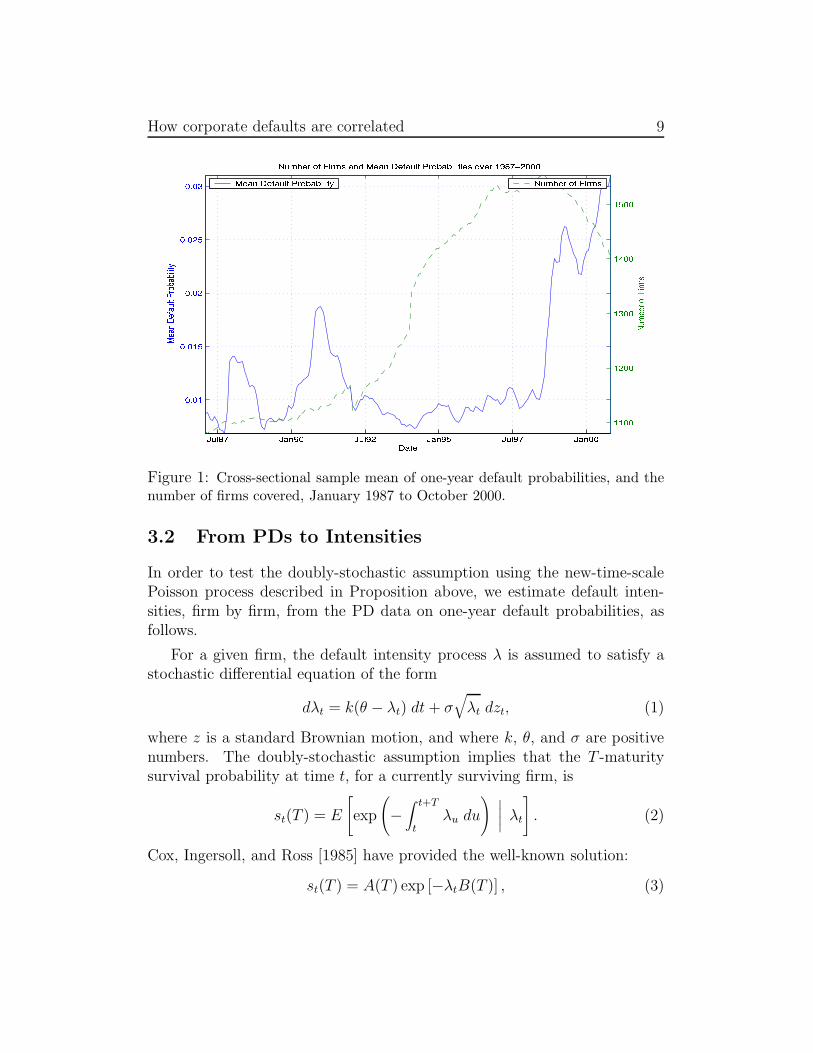
Figure 1 shows a plot of the monthly cross-sectional sample mean ofestimated one-year conditional default probabilities. The plot shows evidenceof positive correlation of default intensities, in that the cross-sectional meanone-year conditional probability of default ranges from 0.69% to 3.11%, andincreases markedly with the U.S. recesssion that occurred around 2000-2001.The number of firms in our sample at a given time increases from a low of1,081 firms at the beginning of the sample period in 1987 to a high of 1,554firms in the second half of 1998. Figure 2 shows a plot of the number ofdefaults over this period, month by month, ranging from 0 to a maximum of8 per month, as well as a plot of the total of the estimated default intensitiesof all sampled firms. We turn next to the estimation of these intensities fromone-year default probabilities.


Figure 1: Cross-sectional sample mean of one-year default probabilities, and thenumber of firms covered, January 1987 to October 2000.

3.2 From PDs to Intensities

In order to test the doubly-stochastic assumption using the new-time-scalePoisson process described in Proposition above, we estimate default inten-sities, firm by firm, from the PD data on one-year default probabilities, asfollows.

For a given firm, the default intensity process λ is assumed to satisfy astochastic differential equation of the form

dλt = k(θ − λt) dt + σ√

λt dzt, (1)

where z is a standard Brownian motion, and where k, θ, and σ are positivenumbers. The doubly-stochastic assumption implies that the T -maturitysurvival probability at time t, for a currently surviving firm, is

st(T ) = E

[

exp

(

−∫ t+T

tλu du

)

∣

∣

∣

∣

λt

]

. (2)

Cox, Ingersoll, and Ross [1985] have provided the well-known solution:

st(T ) = A(T ) exp [−λtB(T )] , (3)


where

A(T ) =

(

2γe(k+γ)T/2

(k + γ)(eγT − 1) + 2γ

)

2kθ

σ2

(4)

B(T ) =2eγT − 1

(k + γ)(eγT − 1) + 2γ(5)

γ =√

k2 + 2σ2. (6)

Inverting equation (3), we get, for any time horizon T ,

λt = − 1

B(T )ln

[

st(T )

A(T )

]

. (7)

Our PD data are data are monthly observations of the one-year defaultprobability, 1− st(1). We estimate the parameters k, θ, σ, and the defaultintensities of each firm, by a method-of-moments estimator provided in Ap-pendix B. The estimator matches the time-series behavior of λt implied bythe Feller diffusion, using the relationship between default intensity and PDgiven by (7). Maximum likelihood estimation has also been used in similarsettings, and is efficient in large samples, but is notoriously biased in smallsamples. Our method-of-moments estimator is robust and computationallyefficient, usually able to fit a given firm’s default intensity model in a coupleof seconds. In any case, the fit is relatively robust to mis-specification ofthe time-series model and to fitting error, as intensities are relatively closeto one-year default probabilities. Figure 2 shows the total of the estimatedintensities of all firms, as well as the monthly arrivals of defaults.

4 Goodness-of-Fit Tests

Having estimated default intensities λit for each firm i and each date t (withλt taken to be constant within months), and letting τ(i) denote the defaulttime of name i, we let U(t) =

∫ t0

∑ni=1 λis1τ(i)>s ds be the total accumulative

default intensities of all surviving firms. Fixing time bins containing c unitsof accumulative default intensity, we then construct calendar times t0, t1,t2, . . . such t0 = 0 and U(ti) − U(ti−1) = c, and let Xk =

∑ni=1 1tk≤τ(i)<tk+1

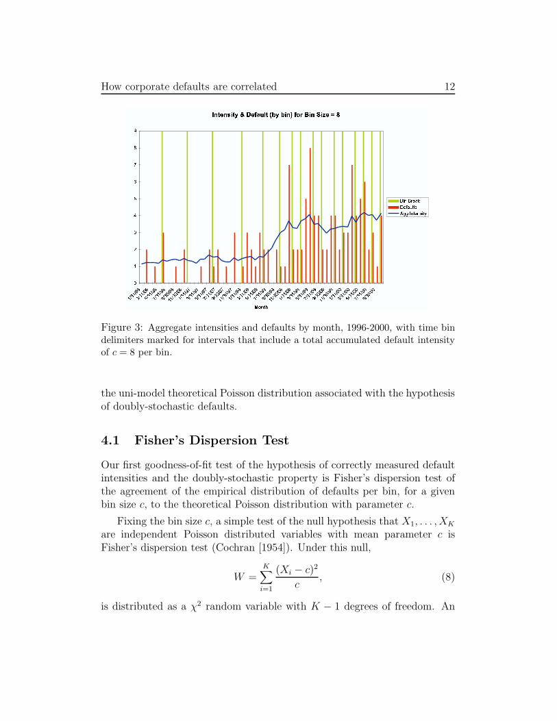
denote the number of defaults in the k-th time bin. Figure 3 illustrates thethe time bins of size c = 8 over the last five calendar years of our data set.


Figure 2: Aggregate (across firms) default intensities and firm defaults from 1987-2000.

Table 1 presents a comparison of the empirical and theoretical momentsof the distribution of defaults per bin, for each of several bin sizes.2 Theactual bin sizes differ very slightly from the integer bin sizes shown be-cause of daily granularity in the construction of the binning times t1, t2, . . ..The approximate match between a bin size and the associated sample mean(X1+· · ·+XK)/K of the number of defaults per bin offers some confirmationthat the underlying PD data are reasonably well estimated, however this isto be expected given the within-sample nature of the estimates. For largerbin sizes, the empirical variances are bigger than their theoretical counter-parts under the null of correctly specified doubly-stochastic intensity modelof defaults.

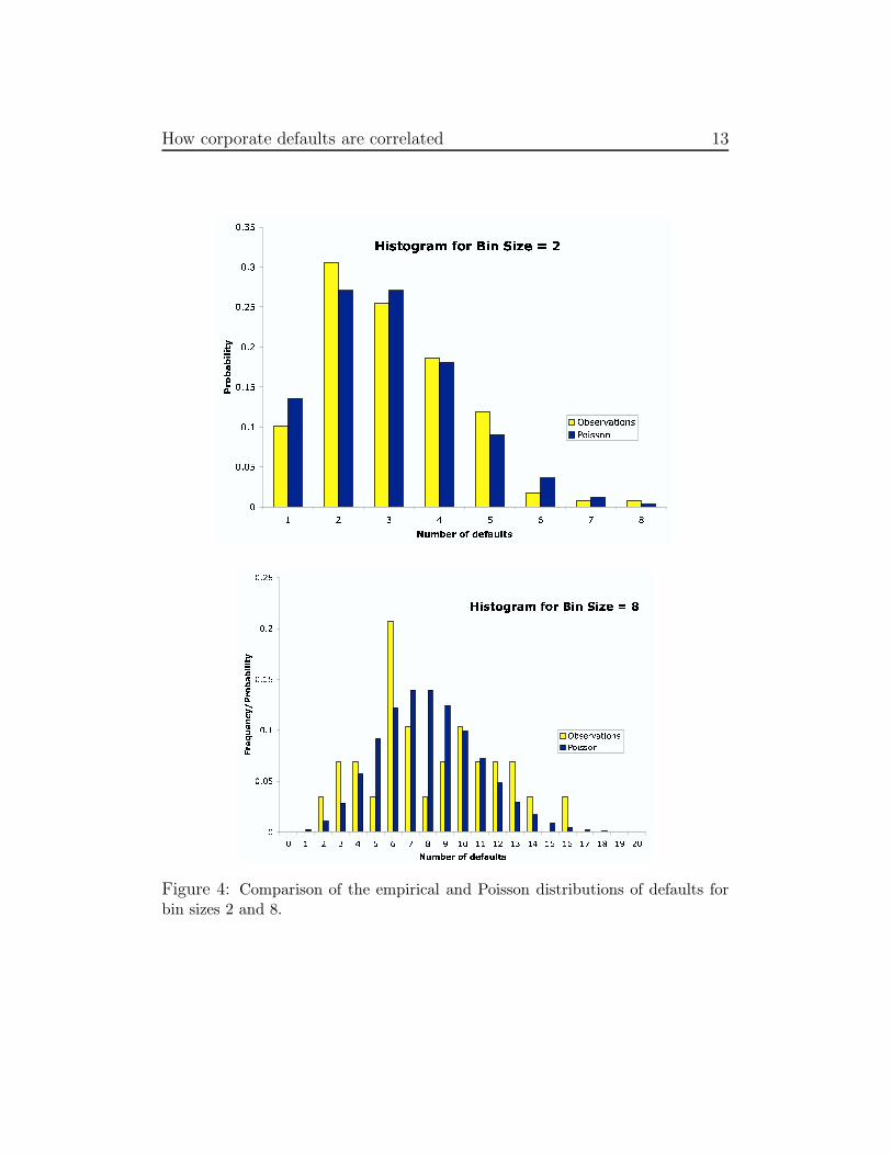
Figure 4 presents the observed default frequency distribution, and theassociated theoretical Poisson distribution, for bin sizes 2 and 8. For binsizes 4 and 8, there is a tendency for bi-modality (two peaks), as opposed to

2Under the Poisson distribution, P (Xi = k) = e−c

ck

k!. The associated moments of Xk

are a mean and variance of c, a skewness of c−0.5, and a kurtosis of 3 + c−1.


Figure 3: Aggregate intensities and defaults by month, 1996-2000, with time bindelimiters marked for intervals that include a total accumulated default intensityof c = 8 per bin.

the uni-model theoretical Poisson distribution associated with the hypothesisof doubly-stochastic defaults.

4.1 Fisher’s Dispersion Test

Our first goodness-of-fit test of the hypothesis of correctly measured defaultintensities and the doubly-stochastic property is Fisher’s dispersion test ofthe agreement of the empirical distribution of defaults per bin, for a givenbin size c, to the theoretical Poisson distribution with parameter c.

Fixing the bin size c, a simple test of the null hypothesis that X1, . . . , XK

are independent Poisson distributed variables with mean parameter c isFisher’s dispersion test (Cochran [1954]). Under this null,

W =K∑

i=1

(Xi − c)2

c, (8)

is distributed as a χ2 random variable with K − 1 degrees of freedom. An


Figure 4: Comparison of the empirical and Poisson distributions of defaults forbin sizes 2 and 8.


Table 1: Comparison of empirical and theoretical moments for the distribution ofdefaults per bin. The number of bin observations is shown in parentheses under thebin size. The upper-row moments are those of the theoretical Poisson distributionunder the doubly-stochastic hypothesis; the lower-row moments are the empiricalcounterparts.

Bin Size Mean Variance Skewness Kurtosis2 2.00 2.00 0.71 3.50

(118) 2.04 1.89 0.71 3.524 4.00 4.00 0.50 3.25

(59) 4.07 4.00 0.41 2.066 6.00 6.00 0.41 3.17

(39) 6.08 8.07 0.41 2.198 8.00 8.00 0.35 3.12

(29) 8.14 13.12 0.26 2.0710 10.00 10.00 0.32 3.10

(24) 10.04 15.43 0.82 2.25

outcome for W that is large relative to a χ2 random variable of the asso-ciated number of degrees of freedom would cause a small p-value, meaninga surprisingly large amount of clustering if the null hypothesis of doublystochastic default (and correctly specified conditional default probabilities)applies. The p-values shown in Table 2 indicate that, at standard confidencelevels such as 95%, there is a borderline rejection of this null hypothesis forbin sizes 6 and 10.

4.2 Upper tail tests

If defaults are more positively correlated than would be suggested by theco-movement of intensities, then the upper tail of the empirical distributionof defaults per bin could be fatter than that of the associated Poisson dis-tribution. We use a Monte Carlo test of the “size” (mean or median) of theupper quartile of the empirical distribution against the theoretical size of theupper quartile of the Poisson distribution, as follows.

For a given bin size c, suppose there are K bins. We let M denote the


Table 2: Fisher’s dispersion test for goodness of fit of the Poisson distributionwith mean equal to bin size. Under the joint hypothesis that default intensitiesare correctly measured and the doubly-stochastic property, W is χ2-distributedwith K − 1 degrees of freedom.

Bin Size K W p-value2 118 110.5 0.654 59 58.0 0.476 39 51.2 0.078 29 46.0 0.02

10 24 35.5 0.05

sample mean of the upper quartile of the empirical distribution of distributionof X1, . . . , XK . By Monte Carlo simulation, we generated 10,000 data sets,each consisting of K iid Poisson random variables with parameter c. Wethen compute the fraction p of the simulated data sets whose sample upper-quartile size (mean or median) is above the actual sample mean M . Underthe null hypothesis that the distribution of the actual sample is Poisson withparameter c, the p-value would be approximately 0.5.

The sample p-values are presented in Table 3, and suggest, for largerbin sizes, fatter upper-quartile tails than those of the theoretical Poissondistribution. (That is, our one-sided tests implies rejection for larger bins ofthe null joint hypothesis, at typical confidence levels.)

We corroborated these results with an analysis of the tail distributionsusing the Pearson χ2 statistic for the theoretical tail distribution associatedwith the corresponding theoretical Poisson distribution. The results (notreported) imply a strong rejection of a Poisson-distributed upper-quartiledistribution at standard confidence levels.

4.3 Prahl’s Test of Clustered Defaults

Fisher’s dispersion and our tailored upper-tail test do not exploit well theinformation available across all bin sizes. In this section, we apply a testfor “bursty” default arrivals due to Prahl [1999]. Prahl’s test is sensitiveto cluster-like deviations from the theoretical Poisson process. This test is


Table 3: Tests of median and mean of the upper upper quartile of defaults perbin, against the associated theoretical Poisson distribution. The last line in thetable, denoted “All” is the probability, under the hypothesis that time-changeddefault arrivals are Poisson with parameter 1, that there exists at least one binsize for which the mean (or median) of number of defaults per bin exceeds thecorresponding empirical mean (or median).

Bin Mean of Tails p-value Median of Tails p-valueSize Data Simulation Data Simulation

2 3.62 3.63 0.58 3.00 3.18 0.254 6.71 6.25 0.21 6.00 5.90 0.176 10.00 8.81 0.05 9.50 8.42 0.078 12.75 11.12 0.03 12.50 10.69 0.03

10 16.00 13.71 0.02 16.50 13.26 0.00All 0.70 0.44

particularly suited for detecting clustering of defaults that may arise frommore default correlation than would be suggested by co-movement of defaultintensities alone.

Prahl’s test statistic is based on the fact that, in the new time scale underwhich default arrivals are those of a Poisson process (with rate parameter 1),the inter-arrival times Z1, Z2, . . . are iid exponential of mean 1. (Because ofdate granularity, our mean is slightly larger than 1.) The sample momentsof these time-rescaled inter-arrival times are provided in Table 4.

Letting C∗ denote the sample mean of Z1, . . . , Zn, Prahl shows that

M =1

n

∑

Zk<C∗

(

1 − Zk

C∗

)

. (9)

is asymptotically (in n) normally distributed with mean e−1 −α/n and vari-ance β2/n, where

α ' 0.1839

β ' 0.2431.

Using our data, for n = 240 default times,

M = 0.3681


Table 4: Selected moments of the distribution of cumulative amount of in-tensities between successive default times. Under the joint hypothesis ofdoubly-stochastic defaults and correctly measured default intensities, the dis-tribution is exponential.

Moment Empirical ExponentialMean 1.07 1.07

Variance 1.19 1.16Skewness 2.13 2.00Kurtosis 7.46 6.00

µ(M) =1

e− α

n= 0.3671

σ(M) =β√n

= 0.0156.

Because the test statistic M is less that one tenth of a standard deviationfrom the associated asymptotic mean, this test provides no notable evidenceof default clustering in excess of that associated with the default intensitiesunder the doubly stochastic model.

We also report a direct Kolmogorov-Smirnov goodness-of-fit test of good-ness of fit the exponential distribution of inter-default times in the new timescale. The associated K-S statistic is 1.8681, for a p-value of only 0.002,leading to a strong rejection of the joint hypothesis of corrrectly specifiedconditional default probabilities and the doubly-stochastic nature of corre-lated default. Figure 5 shows the empirical distribution of inter-default timesafter scaling time change by total intensity of defaults, compared to the ex-ponential density implied by the doubly-stochastic model.

In summary, Prahl’s test does not indicated default clustering in excess ofwhat would be implied by the doublly stochastic property and co-movementof the default intensities.


Figure 5: The empirical distribution of inter-default times after scaling timechange by total intensity of defaults, compared to the exponential density impliedby the doubly-stochastic model.

5 Testing for Independent Increments

Although all of the above tests depend in part on the independent-incrementsproperty of Poisson processes, we will test specifically for serial correlation ofthe number of defaults in successive bins. That is, under the null hypothesisof doubly-stochastic defaults, fixing an accumulative total default intensity ofc per time bin, the number of defaults X1, X2, . . . in successive bins are inde-pendent and identically distributed. We test for independence by estimatingan auto-regressive model for X1, X2, . . ., allowing for Xk = A + BXk−1 + εk,for coefficients A and B, and for iid innovations ε1, ε2 . . .. A large and pos-itive auto-regressive coefficient B would be evidence of a failure of the nullhypothesis. Such a failure in small bins could generate the effect of fat tails inlarger bins, and could be responsible for the apparent rejections of the Pois-son distribution in the larger bins that we reported earlier. Such a failurecould perhaps be evidence of mis-specification of the underlying PD model,for example through missing covariates for default prediction. That is, serialcorrelation of missing covariates could cause an appearanc default clustering


Table 5: Results for AR(1) regressions of defaults of consecutive bins, for each ofa range of bin sizes.

Bin No. of A B R2

Size Bins (tA) (tB) AR(1)

2 118 1.73 0.16 0.03(7.66) (1.72) 0.16

4 59 2.72 0.34 0.12(4.83) (2.73) 0.34

6 39 4.20 0.32 0.10(3.97) (2.01) 0.32

8 29 6.68 0.19 0.03(3.83) (0.96) 0.18

10 24 6.09 0.39 0.15(2.75) (1.93) 0.39

in excess of that implied by the doubly-stochastic property, even if in factthe true default-time model is doubly stochastic.

Table 5 presents the results of this autocorrelation analysis. The AR(1)coefficient is always positive, and sometimes sigificantly larger than zero attraditional confidence levels. Indeed, the auto-regressive coefficient B tendsto be “more significant” for small bin sizes, consistent with an interpretationof the earlier failure of the test for Poisson distributed upper tails in largebins as potentially due to a failure of the independence assumption for smallbins, and perhaps mis-specification of the underlying intensity model.

6 Tests for Missing Default Covariates

Our lack of support for the joint hypothesis of correctly specified defaultprobabilities and the doubly stochastic property might be related to missingcovariates in the PD default-prediction model, a logit-based model that usesonly firm-specific covariates. In particular, this default prediction model maybe missing covariates that are common to many firms, and would thereforereveal additional default time correlation under the doubly-stochastic model.

Prior work by Shumay [2001], Lennox [1999], Lo [1986], and Duffie and


Ke [2003] indeed suggests that macro-economic performance is an importantexplanatory variable in default preduction. Among these prior studies, Duffieand Ke included distance to default, the key covariate in Moody’s PD model,and found significant additional dependence of default intensities on U.S.personal income growth, for the U.S. machinery and instruments sector for1971 to 2001.

In this section, we explore the potential role of two macro-economic vari-ables, United States G.D.P. growth rate (GDP ) and personal income growthrate (PI). In particular, we examine (i) whether the inclusion of these macro-economic variables helps predict defaults in addition to the default intensities,and if so, (ii) whether these variables can potentially explain the apparentfailure of the doubly-stochastic assumption.

We first examine whether the default intensities based on Moody’s defaultintensities indeed indicate mis-specification from lack of a macro-economiccovariate. Under the null hypothesis of no mis-specification, fixing a bin sizeof c, the number of defaults in a bin in excess of the mean, Yk = Xk − c,is the increment of a martingale, and should therefore be uncorrelated withany variable in the information set available prior to the formation of thek-th bin. Consider the regression,

Yk = α + β1PIk + β2GDPk + εk, (10)

where PIk and GDPk are the growth rates of U.S. personal income andU.S. growth in gross domestic product observed in the quarter immediatelyprior to the beginning of the k-th bin. Under the null hypothesis of correctspecification, whether or not the doubly-stochastic assumption is satisfied, thecoefficients β1 and β2 are in theory equal to zero. Table 6 reports estimatedregression results for a range of bin sizes.

We report the results for the multiple regression as well as for each ofthe variables separately. For bin sizes of both 2 and 10, the coefficient forGDP growth rate is significant at the 99% level. For each of the bins, thesigns of the coefficients in the single equation regressions are negative asone would expect under a mis-specification of missing macro-economic vari-ables. That is, significantly more than the number of defaults predictedby the PD model occur when GDP and personal income growth rates arelower than normal. Overall, there appears to be at least some mild evidenceof mis-specification. Given the persistence of macro-economic performanceacross time, these missing covariates may also be partly responsible for the


presence of the apparent auto-correlation in X1, X2, . . . that we reported ear-lier. One may therefore wish to consider whether any excess clustering ofdefaults (beyond that implied by the doubly-stochastic property) is relatedto this potential mis-specification of the default intensity processes. Withthe presently available data, we are unable to disentangle the role of miss-ing covariates from any potential for contagion for the apparently fat taileddistribution of defaults per bin.

Table 7 specifically tests whether the excess upper quartile defaults (de-fined as the mean of the upper quartile less the mean of the upper quartile forthe Poisson distribution of parameter c) examined previously in Table 3 arecorrelated with the personal income and GDP growth rates. We report twosets of regressions, the first set based on the prior period’s macro-economicvariables and the second set based on the growth rates observed within thebin-period.3

As for these upper-tail-size regressions, the estimated coefficients for PIand GDP based on the prior period’s growth rates are not significant attypical confidence levels. The coefficient for current-period PI for bin-size 4,however, is significant at typical confidence levels, and has a sign consistentwith the presence of mis-specification by failure to include macro-economicperformance variables in prediction of default.

7 Concluding Comments

Defaults cluster in time both because firms’ default intensity processes arecorrelated and also perhaps because, even after conditioning on these inten-sities, default occurrence is correlated through additional channels such ascontagion and frailty. The latter channels are not admitted in a doubly-stochastic setting. By a time change that reduces the process of cumulativedefaults to a standard Poisson process, we provide test statistics of the jointhypothesis that default intensities are correctly measured and the doubly-stochastic property. We are particularly interested in whether defaults areindeed independent given intensities. We believe this to be the first suchempirical test. For several types of tests, we reject (at traditional confidencelevels) the null of correctly measured intensities and the doubly-stochastic

3The within-period growth rates are computed by compounding over the daily growthrates that are consistent with the reported quarterly growth rates.


Table 6: Macroeconomic Variables and Default Intensities. For each bin size c,OLS-estimated coefficients are reported for regression of the number of defaultsin excess of the mean, Yk = Xk − c, on the previous quarter’s personal incomegrowth rate and the GDP growth rate. The number of observations is the numberof bins of size c. Standard errors are corrected for heteroskedasticity; t-statisticsare reported in parentheses.

Bin Size No. Bins Intercept Personal Income GDP R2

(%)

2 118 0.10 -11.15 0.37(0.58) (-0.65)0.49 -14.13 5.65

(2.71) (-3.03)0.46 27.37 -19.74 6.98

(2.45) (1.33) (-3.35)

4 59 0.25 -25.39 0.93(0.56) (-0.63)0.76 -21.16 5.74

(1.53) (-1.76)0.74 18.55 -24.85 6.07

(1.43) (0.41) (-1.75)

6 39 0.53 -56.34 2.14(0.69) (-0.73)1.26 -34.38 7.76

(1.45) (-1.58)1.24 6.37 -35.53 7.78

(1.37) (0.08) (-1.49)

8 29 1.06 -28.35 2.93(0.74) (-0.76)0.13 -2.65 0.00

(0.12) (-0.03)0.97 65.44 -42.16 4.28

(0.67) (0.59) (-0.91)

10 24 1.15 -127.60 6.10(0.78) (-0.92)2.62 -71.44 18.99

(1.76) (-1.97)2.57 44.67 -81.00 19.39

(1.61) (0.37) (-2.53)


Table 7: Upper-tail regressions. For each bin size c, OLS-estimated coefficientsare shown for regression of the number of defaults observed in the upper quartileless the mean of the upper quartile of the theoretical distribution (with Poissonparameter equal to the bin size) on the previous and current personal income (PI)and GDP growth rates. The number of observations is the number K of bins.Standard errors are corrected for heteroskedasticity; t-statistics are reported inparentheses.

Bin Size K Intercept Previous Qtr PI Previous Qtr GDP R2

(%)

2 40 -0.05 5.23 0.35(-0.71) (0.49)

-0.10 3.47 1.26(-0.75) (0.84)

-0.09 -7.43 5.54 1.52(-0.71) (-0.48) (0.89)

4 17 0.64 -25.07 10.78(2.42) (-1.53)

0.67 -8.30 9.64(2.52) (-1.48)

0.67 -16.99 -3.52 11.39(2.42) (-0.67) (-0.39)

Bin Size K Intercept Current Bin PI Current Bin GDP R2

(%)

2 40 -0.00 -0.94 0.01(-0.03) (-0.09)

-0.09 3.13 0.97(-0.63) (0.59)

-0.08 -20.53 8.66 2.90(-0.58) (-0.65) (0.71)

4 17 0.69 -32.96 15.71(2.86) (-2.85)0.55 -4.26 2.02

(2.42) (-0.68)0.55 -72.94 17.45 26.50

(2.56) (-2.70) (1.60)


property, at traditional confidence levels. We present some evidence, how-ever, of potential mis-specification of these default probability estimates, inthat they do not include business-cycle covariates that may offer some predic-tive power for default above and beyond the role of firm-specific covariates.Moreover, there is at best weak evidence of highly clustered defaults, aftercontrolling for co-movement in intensities by a time change.

The economic impact of a failure of the doubly-stochastic property forthe risk management of credit portfolios is of critical interest to investorsand bank regulators. For example, the level of economic capital necessary tosupport levered portfolios at high confidence levels is heavily dependent onthe degree to which this often-assumed property actually applies. This is es-pecially the case in light of the upcoming changes in bank capital regulationsunder the proposed Basel II accord on regulatory capital (see Gordy [2003],Allen and Saunders [2003], and Kayshap and Stein [2004]).


Appendices

A Moody’s Data on Defaults

This appendix provides some details of the creation of the data set used in thispaper. Our source of data are two separate databases, one containing defaultprobabilities and the other containing information of defaults. For the empiricalwork in this paper, we need to account for all the defaults that occur over oursample of firms for which we have PDs. Below, we describe how we link the twodatasets, and the set of defaults that results from our procedures.

In its default database, Moody’s records 628 US and Canadian defaults ofnon-financial firms in the period 1/87 to 10/2000. A few firms default twice overthis time period (Grand Union defaulted three times). Moody’s records defaultsonly for firms that it has rated at some point in the firm’s history. The defaultsin the database are indexed by Moody’s Issuer Number (MIN). Although some ofthese firms are linked to a Cusip or a Bloomberg ticker, many of the firms do nothave a link to any external identifier. However, the name of the defaulted firm isprovided, as well as some information regarding the nature of default. Moody’sdatabase of default probabilities is created using accounting and equity price data,and is limited to firms that had available data in the sample period. Our sampleperiod is January 1987 to October 2000. This data is indexed by the Gvkey.

The defaulted firms that have a Cusip are matched to the PD database usingthe Gvkey-Cusip link of the combined Compustat-CRSP database. For the re-maining firms, we do a manual match using the company name. After both thesematches, many firms remain without a Gvkey. Some of these firms do not haveGvkeys because they are either subsidiaries, or related to the primary public firmthat has defaulted. For example, on 7 April 1987, Texaco Capital, Texaco Cap-ital N.V., Texaco Corporation and Texaco Operations Europe are listed as fourseparate defaults. Of these, only Texaco Corporation is counted in our sample.

The number of defaults that are available for our empirical work is fartherreduced as many firms were not rated by Moody’s according to our PD databaseover the period 1987-2000. The final dataset, corresponding to the default of firmsthat are present in the PD database over our sample period, contains 241 incidentsof defaults among a total of 1,990 firms and over 216,859 firm-months of data.


B Estimation of Default Intensities from PDs

This appendix provides the algorithm for our method-of-moments estimator ofdefault intensities.

1. First, we obtain starting coefficient estimates values from the regression, forh = 1/12,

st+h(1) − st(1) = α + βst(1) + et, (11)

where α and β are the ordinary-least-squares (OLS) estimators and et de-notes the residual. From this regression, we get initial estimates of the threeparameters as:

k = −β

h(12)

θ = −α

β(13)

σ =V (e)√

θh, (14)

where V (et) denotes the sample standard deviation of the residual et.

2. Given starting values of k, θ, σ, we obtain an initial estimate of the defaultintensity λt, for each observation time t, using equation (7).

3. Next, we estimate by OLS,

λt+h − λt = a + bλt + wt. (15)

New parameter estimates are then given by

k = − b

h, θ = −a

b, σ = V

(

wt√hλt

)

, (16)

where, again, V ( · ) denotes sample standard deviation.4

4. Given these updated estimates of the parameters k, θ, σ, we return toSteps 2 and 3, and iterate to numerical convergence.

4In the current version of our results, we use V (wt/√

θh) in place of the sample standarddeviation shown in (16), although our tests indicate that this causes minimal distortion inthe estimated intensities.


References

[2003] Allen, L. and A. Saunders (2003) “A Survey of Cyclical Effects inCredit Risk Measurement Models,” BIS Working Paper 126, BaselSwitzerland.

[1986] Billingsley, Patrick (1986). Probability and Measure, Second Edition,New York: Wiley.

[2002] Cathcart, L. and L. El Jahel (2002) “Defaultable Bonds and DefaultCorrelation,” Working Paper, Imperial College.

[1954] Cochran, W.G. (1954) “Some Methods of Strengthening χ2 Tests,”Biometrics v10, 417-451.

[2003] Collin-Dufresne, Pierre, Goldstein, Robert, and Jean Helwege (2003)“Is Credit Event Risk Priced? Modeling Contagion via the Updating ofBeliefs,” Working Paper, Haas School, University of California, Berkeley.

[2002] Collin-Dufresne, Pierre, Goldstein, Robert, and Julien Huggonier(2002) “A General Formula for Valuing Defaultable Securities,” WorkingPaper, Carnegie-Mellon University.

[1985] Cox, John, Jon Ingersoll, and Steven Ross (1985) “A Theory of theTerm Structure of Interest Rates,” Econometrica v53, 385-407.

[2001] Das, Sanjiv., Laurence Freed, Gary Geng, and Nikunj Kapadia (2001).“Correlated Default Risk,” working paper, Santa Clara University.

[2000] Davis, Mark, and Violet Lo (2000) “Infectious Default,” Working Pa-per, Imperial College.

[2003] Duffie, D., and Ke Wang (2003). “Multi-Period Corporate Failure Pre-diction with Stochastic Covariates,” working paper, Stanford University.

[2002] Giesecke, Kay (2002) “Correlated Default with Incomplete Informa-tion,” Working Paper, Humboldt University, Berlin.

[2003] Gordy, Michael (2003) “A Risk-Factor Model Foundation for Ratings-Based Capital Rules,” Journal of Financial Intermediation, v12, 199-232.


[2001] Jarrow, R., and Fan Yu (2001). “Counterparty Risk and the Pricingof Defaultable Securities,” Journal of Finance 56, 1765-1800.

[1999] Jarrow, R., David Lando, and Fan Yu (1999). “Default Risk and Di-versification: Theory and Applications,” working paper, Cornell Univer-sity.

[2004] Kayshap, A., and J. Stein (2004) “Cyclical Implciations of the Basel-II Capital Standards,” Working Paper, Graduate School of Business,University of Chicago.

[1999] Kusuoka, Shigeo (1999) “A Remark on Default Risk Models,” Ad-vances in Mathematical Economics v1, 69-82.

[1994] Lando, David (1994). “Three essays on contingent claims pricing,”Ph.D. thesis, Cornell University.

[1998] Lando, David (1998). “On rating transition analysis and correlation,”Credit Derivatives: Applications for Risk Management, Investment andPortfolio Optimization, Risk Publications, 147-155.

[1992] Lang, Larry and Rene Stulz (1992), “Contagion and competitive intra-industry effects of bankrtuptcy announcements, Journal of FinancialEconomics v32, 45-60.

[1999] Lennox, C. (1999) “Identifying Failing Companies: A reevaulationof the Logit, Probit, and DA Approaches,” Journal of Economics andBusiness, v51, 347-364.

[1986] Lo, Andrew (1986) “Logit versus Discriminant Analysis: SpecificationTest and Application to Corporate Bankruptcies,” Journal of Economet-rics, v31, 151-178.

[1974] Merton, Robert C. (1974). “On the Pricing of Corporate Debt: TheRisk Structure of Interest Rates,” The Journal of Finance, v29, 449-470.

[1999] Prahl, J. (1999) “A Fast Unbinned Test on Event Clustering in Pois-son Pricesses,” Working Paper, University of Hamburg, submitted toAstronomy and Astrophysics.

[2003] Protter, Philip (2003). Stochastic Integration and Differential Equa-tions, Second Edition (New York: Springer).


[2002] DeServigny, Arnaud, and Olivier Renault (2002) “Default Correlation:Empirical Evidence,” Working Paper, Standard and Poors.

[2004] Schonbucher, Philipp (2004) “Frailty Models, Contagion, and Infor-mation Effects,” Working Paper, ETH, Zurich.

[2001] Schonbucher, Philipp, and D. Schubert (2001) “Copula DependentDefault Risk in Intensity Models,” Working Paper, Bonn University.

[2001] Shumway, Tyler (2001) “Forecasting Bankruptcy More Accurately: ASimple Hazard Model,” Journal of Business v74, 101-124.

[2000] Sobehart, J., R. Stein, V. Mikityanskaya, and L. Li, (2000). “Moody’sPublic Firm Risk Model: A Hybrid Approach To Modeling Short TermDefault Risk,” Moody’s Investors Service, Global Credit Research, Rat-ing Methodology, March.

[2000] Sobehart, J.R., Keenan, S.C. and Stein, R.M. (2000), “BenchmarkingQuantitative Default Risk Models: A Validation Methodology,” Techni-cal Report, Moody’s Risk Management Services.

[2003] Terentyev, S. (2004) “Asymmetric Counterparty Relations in DefaultModeling,” Working Paper, Department of Stastistics, Stanford Univer-sity.

[1987] Vasicek, Oldrich (1987) “Probability of Loss on Loan Portfolio,”Working Paper, KMV Corporation.

[2003] Yu, Fan (2003) “Default Correlation in Reduced Form Models,” Work-ing Paper, U.C. Irvine.

[2004] Yu, Fan (2004) “Accounting Transparency and the Term Structure ofCredit Spreads,” Working Paper, U.C. Irvine.

[2001] Zhou, C. (2001) “An Analysis of Default Correlation and MultipleDefauls,” Review of Financial Studies, Vol. 14, pp. 555-576.

Documents

Common Failings: How Corporate Defaults are Correlated