Commodity Prices and Growth: Reconciling a Conundrum1

Paul Collier and Benedikt Goderis

Department of Economics,

University of Oxford

January, 2007

Abstract

Currently, evidence on the ‘resource curse’ yields a conundrum. While there is much informal evidence to support the ‘curse’ hypothesis, time series analyses using the VAR methodology have found that increases in commodity prices significantly raise the growth of commodity exporters. We adopt co-integration methodology, enabling us to explore longer term effects than permitted using VARs, and analyze a global data set covering 1971-2004. We find sharp differences in the effects, both between the short term and the long term, and the type of commodity. For all types of commodity, the short term consequences of price booms are benign for their exporters: the direct gain from the income terms of trade is reinforced by induced growth in constant-price GDP. For agricultural commodities the output effect persists over the long term. However, for both oil and the other non-agricultural commodities, the long term effects on output are adverse and substantial. Our results thus support the ‘resource curse’ hypothesis, while reconciling the apparent inconsistency with results based on VARs. Keywords: commodity prices; natural resource curse; growth

JEL classification: O13, O47, Q33

1 We would like to thank Chris Adam, Kofi Adjepong-Boateng, Mardi Dungey, Ron Smith, Måns Söderbom and participants at the UNU-WIDER Conference “Aid: Principles, Policies, and Performance”, Helsinki, June 2006, for useful comments. Any remaining errors are our own.

2

1. Introduction

A large but predominantly informal literature suggests that there is a ‘resource curse’:

natural resource abundant countries tend to grow slower than resource-scarce

countries.2 The theoretical literature has suggested three possible channels of

transmission. First, countries with natural resources often face more volatility,

especially through commodity prices. Second, increases in commodity prices can lead

to Dutch Disease effects. And finally, natural resources can have adverse effects on

governance.3 In all three channels, the effect of commodity revenue windfalls is

crucial. Such windfalls can occur both through the discovery of natural resources and

through commodity booms.

Whereas the resource curse theory predicts a negative effect of commodity booms on

growth, recent empirical studies by Deaton and Miller (1996) for Africa and Raddatz

(2005) for low-income countries find quite the contrary: commodity booms

significantly raise growth. The rise in African growth rates during the commodity

boom that began in 2000 is clearly consistent with the results of Deaton and Miller

and Raddatz. However, an acknowledged limitation of the VAR technology deployed

in these studies is that it cannot address long-run effects. It is therefore possible that

the positive short-run effects are offset by a subsequent resource curse beyond the

horizon of the VAR approach: the post-2000 upturn would be a false dawn. In this

paper we adopt cointegration methodology to analyze global data for 1971-2004 to

disentangle the short and long run effects of commodity prices on growth.

The rest of this paper is structured as follows. Section 2 describes the empirical

analysis, including the cointegration tests. In Section 3 we set out the results of the

cointegration analysis and use them to simulate the short and long run effects of

higher commodity export prices on growth in commodity-dependent economies.

While the short run effects are fully consistent with those of earlier studies, we find

that in the long run for oil and other non-agricultural commodities there is indeed a 2 Sachs and Warner (1995, 1997a, b), Leite and Weidmann (1999), Auty (2001), Bravo-Ortega and De Gregorio (2001), and Sala-i-Martin and Subramanian (2003). 3 Models of Dutch Disease were first introduced by Corden and Neary (1982) and Van Wijnbergen (1984). For the adverse effects on governance, see the rent-seeking models by Lane and Tornell (1996), Tornell and Lane (1999) and Torvik (2002).

3

significant and substantial resource curse. In Section 4 we test two of the transmission

channels of the resource curse effect, as suggested by the theoretical literature: Dutch

disease and volatility. We find that Dutch disease plays a minor role, whereas

volatility may be more important. However, an implication of the result that the

resource curse is confined to non-agricultural commodities, is that governance is

likely to be the critical route. Typically, non-agricultural windfalls accrue

predominantly to governments whereas agricultural windfalls accrue primarily to the

private sector. In Section 5 we apply our results to the present commodity boom in

Africa, disaggregating the accelerated growth of recent years into that attributable to

the short term effects of the commodity boom and that attributable to underlying

changes. Section 6 concludes.

2. The Empirical Analysis

In this section we discuss our choice of statistical technique, the variables we use in

estimation, and the cointegration tests we performed. Data description and sources

can be found in the Appendix.

The short-run and long-run effects of commodity export prices on GDP per capita are

analyzed using the following equilibrium correction model:

tintintiktititiiti uSXYXYY ,,4,3,21,11,, ++∆+∆+++=∆ −−−−− ββββλα (1)

where tiY , is log real GDP per capita in country i in year t and αi is a country-specific

fixed effect. 1, −tiX is a vector of variables (all in logs) that is expected to affect GDP

per capita both in the short run and long run. First, we include our constructed

commodity export price index to test the effect of export prices. We also experiment

with an oil export price index and with separate indices for oil, agricultural, and other

commodities to investigate the effects of different types of commodities. In all

regressions we include an oil import price index to control for the effect of oil prices

on oil importing countries. In addition, we include several control variables, all taken

from the empirical growth literature: i) trade openness, measured as the ratio of trade

4

to GDP, ii) external debt to GNI, iii) inflation, measured as the consumer price index

(cpi), and iv) financial development, measured as the ratio of M2 to GDP.

ntiS −, is a vector of control variables that is expected to have a short-run effect on

growth. This vector includes indicators of civil war and coup d’etat(s). Following

Raddatz (2005) we also control for several types of natural shocks, in particular

geological, climatic, and human disasters. The lag order of the short-run growth

determinants is denoted by k > 0 and n ≥ 0. The paper’s hypotheses are tested through

the short-run and long-run effects of the commodity export price indices, captured

within the coefficient vectors 1β and 3β .

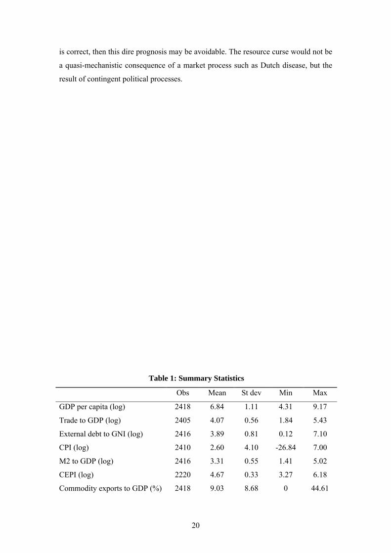
Our dataset consists of all countries and years for which data are available, and covers

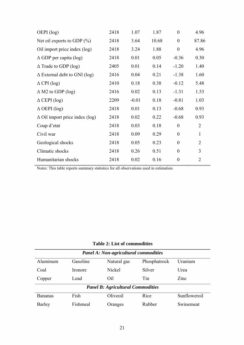
around 100 countries between 1971 and 2004. Table 1 reports summary statistics for

the variables used in estimation. Next, we discuss how the commodity price indices

were constructed.

Constructing commodity price indices

The commodity export price index (CEPI) was constructed using the methodology of

Deaton and Miller (1996) and Dehn (2000). In particular, we collected data on world

commodity prices and commodity export values for as many commodities as data

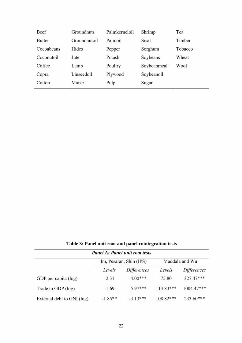
availability allowed. Table 2 lists the 58 commodities in our sample. For each of the

countries, we calculate the total value of commodity exports in 1990. We construct

weights by dividing the individual 1990 export values for each commodity by this

total. These 1990 weights are then held fixed over time and are applied to the world

price indices of the same commodities to form a country-specific geometrically

weighted index of commodity export prices.

When testing for the effect of commodity export prices, it is important that the

commodity export price index is exogenous, i.e. not correlated with the error term in

equation (1). As argued in Deaton and Miller (1996), one of the advantages of using

international commodity prices is that they are typically not affected by the actions of

individual countries. Also, by keeping the weights constant over time, supply

5

responses to price changes are not included. As a result, we believe the index to be

exogenous with respect to GDP or the determinants of GDP.

The oil export and oil import price indices were constructed as follows. We first

collected an index of world oil prices. After taking the log of this index we interacted

it with dummy variables for net oil importing countries and net oil exporting

countries. This yielded two variables. The first, the oil import price index, equals the

log world oil price index for net oil importers and equals zero for net oil exporters.

The second, the oil export price index (OEPI), equals the log world oil price index for

net oil exporters and equals zero for net oil importers.

Testing for cointegration

Using equation (1) above, the long-run equilibrium equation of log real GDP per

capita can be written as follows:

)(1,,1i, titiiti XtY ηβθγ

λ+++−= (2)

where iγ is a country-specific fixed effect and t is a time trend. Note that both the

constant and the coefficient on the time trend are allowed to differ across countries.

This follows from the fact that we left the country-specific fixed effect αi in equation

(1) unrestricted. Hence, it not only captures the country-specific constant iγ in the

levels equation (2) but also the country-specific constant in the differenced equation

(1). The latter implies a country-specific linear time trend in the levels equation (2).

Equation (1) allows us to estimate the long-run relationship in equation (2) if tiY , and

tiX , are cointegrated, i.e. if tiY , and tiX , have a common stochastic trend which is

cancelled out by the linear combination. To test whether the variables do cointegrate,

we first performed panel unit root tests on both the levels and the differences of the

individual variables in tiY , and tiX , and then performed a panel cointegration test. We

use the panel unit root tests by Im, Pesaran and Shin (2003, IPS hereafter) and

Maddala and Wu (1999). Both tests are based on augmented Dickey-Fuller (ADF)

6

tests for the individual series in the panel. This ensures that in both tests the ADF test

statistic is allowed to vary across groups, unlike for example the panel unit root test

by Levin, Lin and Chu (2002). The null hypothesis is that all groups have a unit root

while under the alternative one or more groups do not have a unit root. The IPS test

and the Maddala and Wu test differ in that the first test is parametric and is based on

the t-statistics of the individual unit root tests, whereas the second is non-parametric

and is based on the p-values of the individual unit root tests. The oil export price

index (OEPI) and the oil import price index are either equal to zero or equal to the

world oil price index, which is not country-specific. Hence, a panel unit root test is

not appropriate. Instead, we perform a Dickey-Fuller test on the log world oil price

index series to test for the stationarity of the oil export and import price indices.

In order for the variables to be cointegrated, they should be integrated of order 1, that

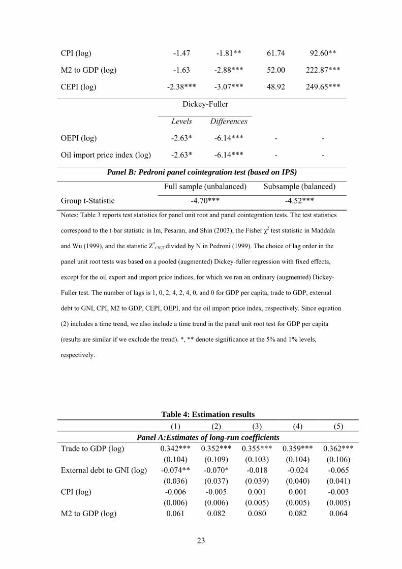
is non-stationary in levels but stationary in first differences. Panel A of Table 3 shows

the results of the panel unit root tests. Most of the results confirm that the series are

I(1). For the differenced series, both the IPS and the Maddala and Wu tests always

reject the null that all groups have a unit root. For the oil price indices, the Dickey-

Fuller test for the differences also rejects the null of a unit root. For most of the level

tests, the null hypothesis that all groups have a unit root is not rejected. However, this

is not always the case. The tests give mixed results for trade to gdp and the

commodity export price index (CEPI), where one of the tests rejects the null and the

other does not. For the oil price indices the null of a unit root is rejected, but only at

the 10 percent level. Finally, both tests reject the null for the external debt to GNI

variable. It is important to point out that these tests only address the null hypothesis

that all series in the panel are non-stationary. Rejection of this null does not mean that

all the individual series are stationary but only that at least one of the series is

stationary.

We next perform a panel cointegration test, as suggested by Pedroni (1999). In

particular we use the Group t-Statistic, which is analogues to the IPS test above but

applied to the estimated residuals of the cointegrating regression. If the variables

cointegrate, the residuals from equation (2) above should be stationary. To construct

the test statistic, we proceed as suggested by Pedroni (1999). We first run the

following regression for each country separately:

7

titt XtY ,210 εααα +++= (3)

where tY is log real GDP per capita and tX includes the long-run GDP determinants

that enter our main specification in columns (1) and (2) of Table 2A below, i.e. log

trade to GDP, log external debt to GDP, log CPI, log M2 to GDP, log CEPI, and log

oil import price index. This allows for country-specific fixed effects, country-specific

time trends and country-specific coefficients for the long-run GDP determinants. We

then collect the residuals from these regressions and run ADF regressions for each

country. Following Pedroni (1999), we allow the number of lagged differences in the

individual ADF regressions to differ across countries by including the lags that enter

statistically significant. Finally, we calculate the average of the ADF t-statistics from

these regressions, which we report in Panel B of Table 3, for both the full unbalanced

sample of 96 countries and a balanced subsample of 33 countries.4 This average is

analogues to the t-bar statistic in the IPS panel unit root test. Importantly, however,

the critical values for the cointegration test differ from the critical values for the IPS

panel unit root test. Pedroni (1999) provides the adjusted critical values. Both the test

for the balanced panel and the test for the full unbalanced panel strongly reject the

null hypothesis that the residuals of the cointegrating regression are non-stationary for

all groups. This supports the hypothesis that the individual series are cointegrated.

3. Estimating the Short and Long Run Effects on Growth

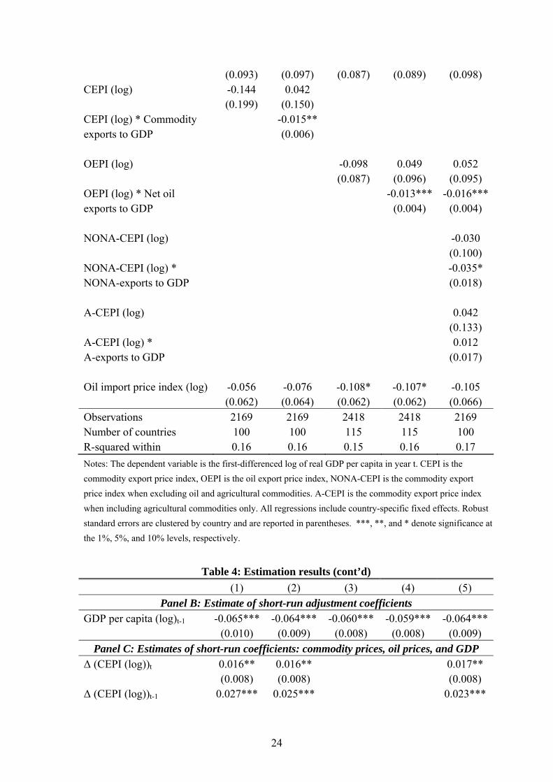
Table 4 reports the results of estimating equation (1) and contains four panels. Panel

A shows the estimates of the long-run coefficients, corresponding to 11 βλ•− in

equations (1) and (2). Panel B reports the estimates of the short-run adjustment

coefficient λ (speed of adjustment). Panel C shows the estimates of the short-run

coefficients for our export price indices ( 3β ) and the lags of the dependent variable

( 2β ). Finally, panel D reports the estimates of the short-run coefficients for our

4 The tests in Pedroni (1999) are developed for balanced panels. However, for sensitivity we also performed the procedure for our full unbalanced sample. Results are similar.

8

control variables ( 3β and 4β , respectively). The five columns in Table 4 correspond

to five different specifications.

The first specification simply includes our commodity export price index (CEPI),

entered directly. As shown in Panel A, the index is not statistically significant.

However, we would expect the consequences of commodity prices to be broadly

proportionate to the importance of commodity exports in GDP. Hence, in column (2)

of Table 4 we add an interaction term of the commodity export price index and the

ratio of commodity exports to GDP. We now find clear evidence of a long run effect.

The interaction term is significant at 5 percent, consistent with the hypothesis of

approximate proportionality. The sign of the coefficient is negative, consistent with a

long-run ‘resource curse’ effect: in the long run higher export prices significantly

reduce the level of constant price GDP in countries with large commodity exports.

Figure 1 illustrates this effect, showing the range of dependence upon commodity

exports over which the adverse effect is significant. As could be expected, countries

with commodity exports close to zero percent of GDP are not affected by higher

commodity prices, i.e. the elasticity of GDP per capita with respect to commodity

prices is approximately zero. For higher levels of commodity exports to GDP, the

elasticity turns negative. For countries with commodity exports to GDP ratios of 19

percent and higher, the negative effect is statistically significant at the 5 percent level.

An example of a country that highly depends on its commodity exports is Zambia. In

1990 Zambia’s commodity exports represented 35 percent of its GDP. The results in

Figure 1 therefore predict a long-run elasticity of -0.47. In other words, a 10 percent

increase in the price of Zambian commodity exports leads to a 4.7 percent lower long-

run level of GDP per capita. These results clearly suggest the existence of a long-run

“resource curse”. We should note that a reduction in constant-price GDP is not the

same as a reduction in real income. The higher export price directly raises real income

for a given level of output and this qualitatively offsets the decline in output. The

magnitude of this benefit from the terms of trade follows directly from the change in

the export price and the share of exports in GDP. Thus, in the example of Zambia

above, the terms of trade gain directly raises income by 3.5 percent of GDP for given

output. Even so, this is less than the decline in output of 4.7 percent, so that the

resource curse ends up reducing both output and income relative to counterfactual.

9

We next investigate whether this adverse long-run effect is common to all the

commodities in our index. Economically the most important commodity in the index

is oil. We replace our general commodity export price index (CEPI) by our oil export

price index (OEPI). Column (3) shows the results when we repeat the specification of

column (1), simply entering the oil export price index directly. As shown in panel A,

the level of the index is again statistically insignificant. As before, we next investigate

whether the long-run effect of higher commodity export prices is proportionate to the

value of oil exports. Hence, in column (4) of Table 4 (panel A) we add an interaction

term of the oil export price index and the net oil exports to GDP ratio. We now find

strong evidence that oil exports have a long-run effect, the interaction term entering

significant at 1 percent. The sign of the coefficient is negative, consistent with the

hypothesis of an ‘oil curse’.

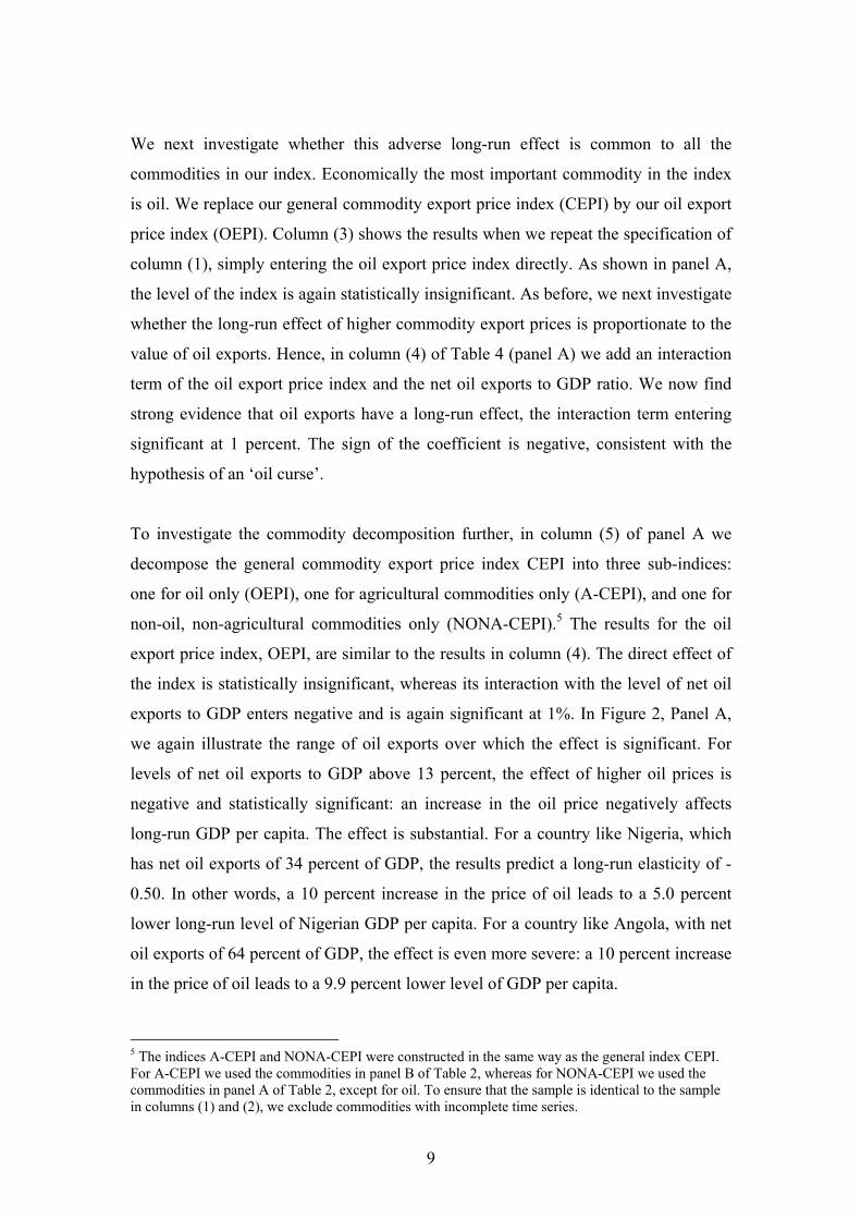
To investigate the commodity decomposition further, in column (5) of panel A we

decompose the general commodity export price index CEPI into three sub-indices:

one for oil only (OEPI), one for agricultural commodities only (A-CEPI), and one for

non-oil, non-agricultural commodities only (NONA-CEPI).5 The results for the oil

export price index, OEPI, are similar to the results in column (4). The direct effect of

the index is statistically insignificant, whereas its interaction with the level of net oil

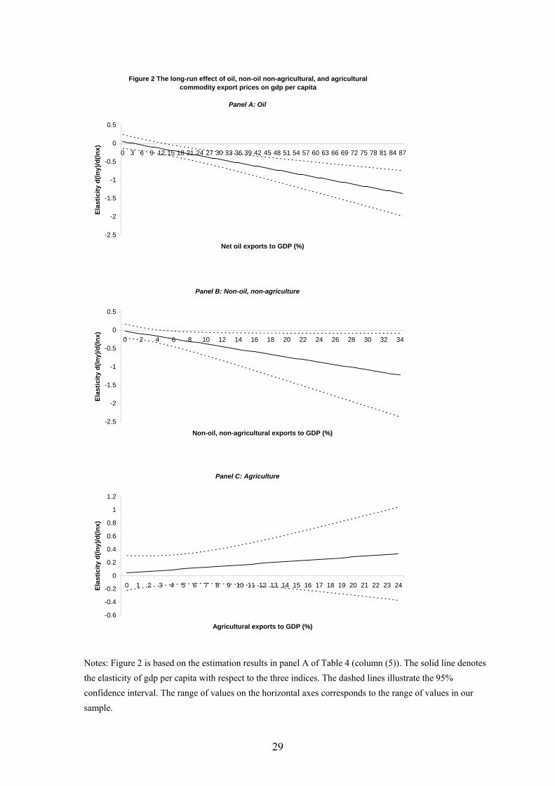
exports to GDP enters negative and is again significant at 1%. In Figure 2, Panel A,

we again illustrate the range of oil exports over which the effect is significant. For

levels of net oil exports to GDP above 13 percent, the effect of higher oil prices is

negative and statistically significant: an increase in the oil price negatively affects

long-run GDP per capita. The effect is substantial. For a country like Nigeria, which

has net oil exports of 34 percent of GDP, the results predict a long-run elasticity of -

0.50. In other words, a 10 percent increase in the price of oil leads to a 5.0 percent

lower long-run level of Nigerian GDP per capita. For a country like Angola, with net

oil exports of 64 percent of GDP, the effect is even more severe: a 10 percent increase

in the price of oil leads to a 9.9 percent lower level of GDP per capita.

5 The indices A-CEPI and NONA-CEPI were constructed in the same way as the general index CEPI. For A-CEPI we used the commodities in panel B of Table 2, whereas for NONA-CEPI we used the commodities in panel A of Table 2, except for oil. To ensure that the sample is identical to the sample in columns (1) and (2), we exclude commodities with incomplete time series.

10

We next investigate the effect of the non-oil, non-agricultural commodities. The direct

effect of this export price index, NONA-CEPI, is again statistically insignificant while

its interaction with the ratio of non-oil, non-agricultural exports to GDP is statistically

significant at 10%6. The sign of the coefficient is again negative, suggesting that the

“resource curse” effect is not confined to oil but also applies to other non-agricultural

commodities. Panel B of Figure 2 illustrates the range over which the effect is

significant, namely once these exports exceed 5 percent of GDP. In this range an

increase in non-oil, non-agricultural commodity export prices leads to lower long-run

levels of per capita GDP. Examples of countries that depend on this class of export

commodities, are Bolivia (10% of GDP), Mauritania (22% of GDP), and Zambia

(34% of GDP). For Mauritania, the results in panel B of Figure 2 predict a long-run

elasticity of -0.80. In other words, a 10 percent increase in the price of non-oil, non-

agricultural commodities, causes an 8.0 percent lower level of per capita GDP.

Finally we investigate the effect of agricultural commodity export prices. As

previously, the direct effect of the index, A-CEPI, is not statistically significant. Now,

however, the interaction term of A-CEPI with the ratio of agricultural exports to GDP

is also insignificant and indeed enters positive. This suggests that higher agricultural

export prices are not a ‘curse’ analogous to non-agricultural commodities: on the

contrary, they are more likely than not to be beneficial. The absence of any “resource

curse” effect for agriculture is illustrated in panel C of Figure 2. The contrast between

the effects of the agricultural and non-agricultural commodities offers a clue as to the

routes by which the latter are having adverse effects. We return to this issue after

discussing the other results.

Having discussed the long-run effects of commodity prices, we now turn to the other

variables in our model. To save space, we only discuss the results in column (1). First,

all of the other long-run determinants enter with the expected signs. Trade to GDP

enters with a positive sign and is statistically significant at the 1% level, indicating

that more open countries tend to have higher long-run GDP levels. External debt

enters negative and significant at the 5% level, indicating that fiscal imprudence has a

negative long-run effect on GDP. The consumer price index enters with the negative 6 When running the specification in column (5) without the agricultural index A-CEPI, the interaction term of NONA-CEPI with the NONA exports to GDP ratio is negative and significant at 5 percent.

11

sign, suggesting that countries with historically high levels of inflation have lower

long-run GDP levels. However, this coefficient is not statistically significant so

should be viewed with caution. The same goes for the ratio of M2 to GDP, which

enters with a positive sign, indicating that more financially developed countries tend

to have higher long-run GDP levels.

Panel B shows the short-run adjustment coefficient that corresponds to the speed of

adjustment to long-run equilibrium. Lagged GDP per capita enters negative and is

statistically significant at the 1% level. The size of the coefficient suggests that the

speed of adjustment (i.e., the proportion of the deviation from steady state that is

corrected) is 6.5 percent per year.

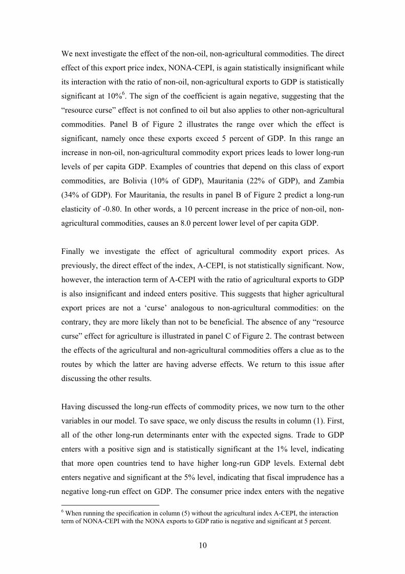
Having considered the long-run effects we now turn to the short-run effects. Column

(1) in panel C reports the short-run coefficients of our commodity export price index

and lagged growth. The results show that the contemporaneous as well as the first

three lags of the change in the log commodity export price index enter positive and

significant at 10 percent or higher, suggesting that an increase in the growth rate of

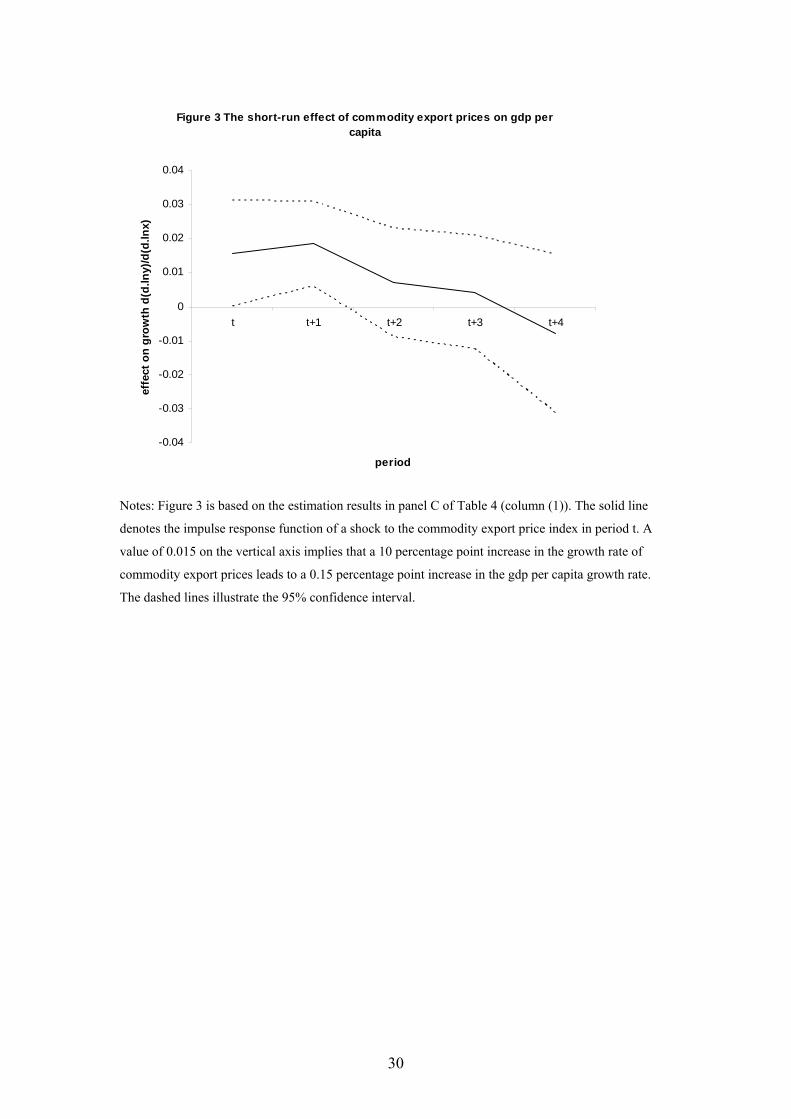
export prices has a positive short-run effect on GDP growth. Figure 3 illustrates this

effect by showing the impulse response function of an increase in the growth rate of

commodity export prices. The effect of a 10 percentage points increase in prices

cumulates to almost 0.5 percentage point of GDP growth after year t+3. The positive

short-run effect of commodity export prices is consistent with the findings in Deaton

and Miller (1996) and Raddatz (2005).7 In addition to the effect of export prices,

column (1) in panel C shows the coefficients of the lags of the dependent variable

GDP growth. We find that the first lag is most important as it enters positive and

significant at 1 percent. The fourth lag enters negative and significant at 5 percent,

suggesting that there is some degree of mean reversion in the growth rate of GDP.

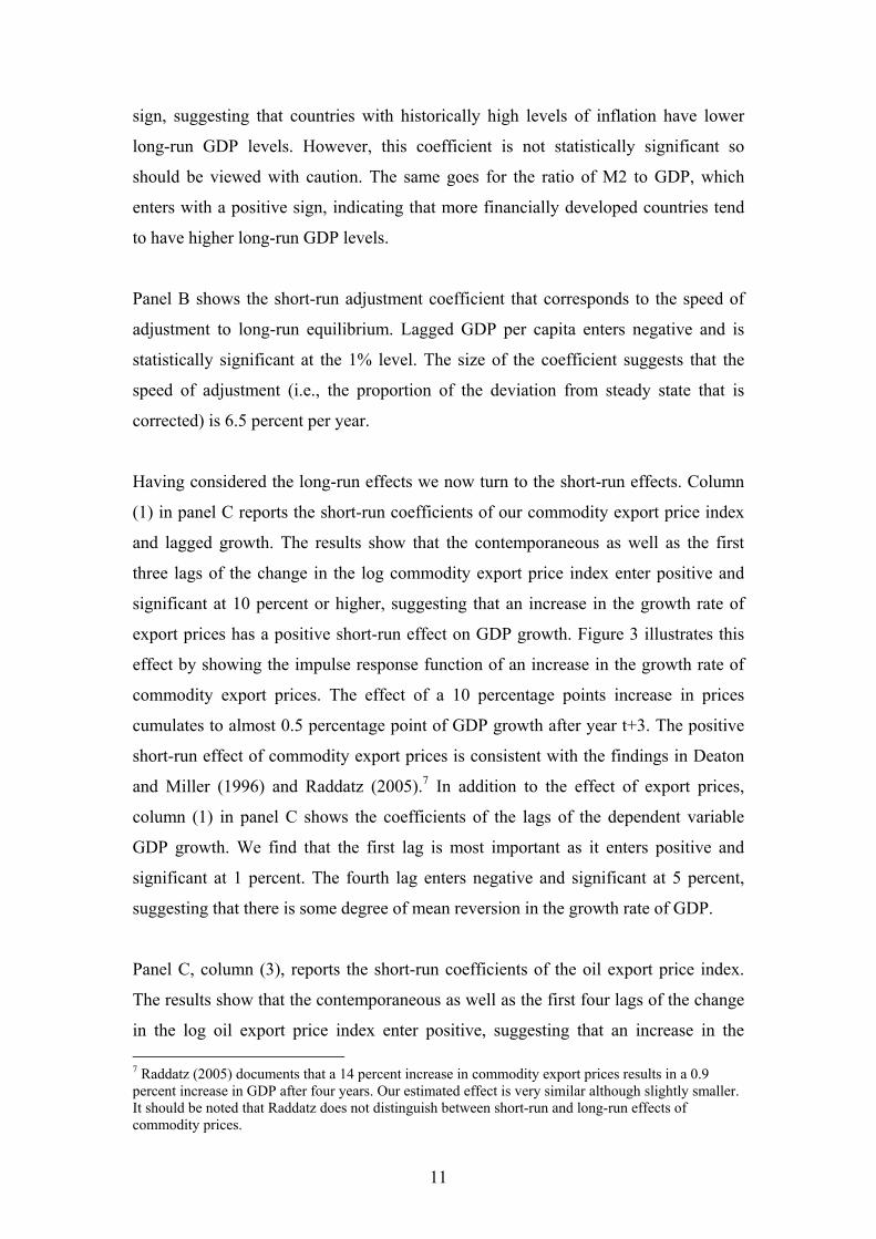
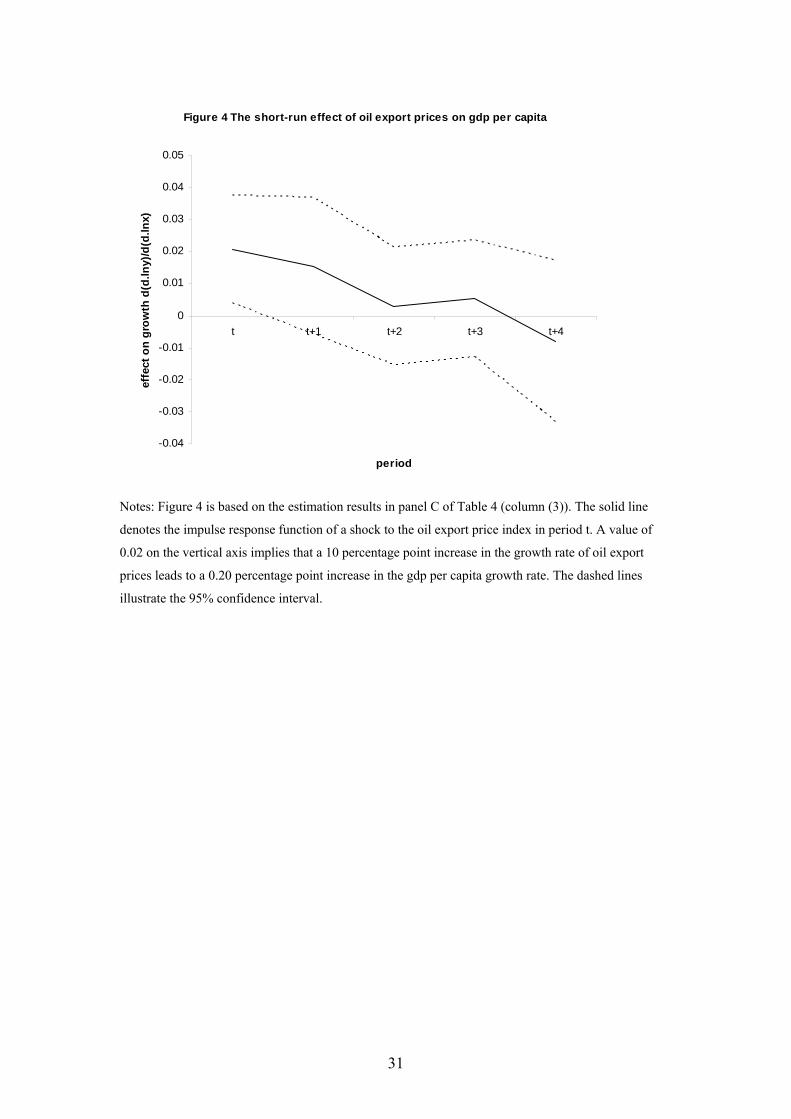
Panel C, column (3), reports the short-run coefficients of the oil export price index.

The results show that the contemporaneous as well as the first four lags of the change

in the log oil export price index enter positive, suggesting that an increase in the 7 Raddatz (2005) documents that a 14 percent increase in commodity export prices results in a 0.9 percent increase in GDP after four years. Our estimated effect is very similar although slightly smaller. It should be noted that Raddatz does not distinguish between short-run and long-run effects of commodity prices.

12

growth rate of oil export prices has a positive short-run effect on GDP growth in oil

exporting countries. However, the effect is only statistically significant in the same

year as the shock. Figure 4 illustrates the short-run effect of higher oil prices by

showing the impulse response function of an increase in the growth rate of oil export

prices. The effect is very similar to the general effect of higher commodity export

prices. A 10 percentage points increase in the oil price cumulates to almost 0.5

percentage points higher GDP growth after year t+3.

Thus, the short-run dynamics of a commodity boom are quite contrary to the long-run

effects. Further, the short run effects on output are reinforced by the direct gain in

income through the improvement in the terms of trade, so that real incomes rise

strongly.

We next discuss the short-run effects of the control variables that were part of the

cointegrating vector (column (1) in panel D). Again, the openness indicator has the

strongest impact on per capita GDP, with up to three lags entering positive and

statistically significant at 10 percent or higher, suggesting that changes in openness

have a positive impact on growth in the following three years. Changes in inflation

have a negative effect on growth in the following year but this effect is reversed in the

third year after the shock. External debt and financial development do not seem to

have short-run effects on growth. A change in the oil price has a negative effect on

growth in oil importing countries in the same year and the three subsequent years,

although this effect is only statistically significant (at 10 percent) in the first year after

the shock.8

The coefficients for the short-run control variables are reported in the remainder of

panel D. The two political shocks, coups and civil war, have large adverse effects on

growth. A coup appears to cut growth by around 2.8 percentage points in the year of

the coup. The negative impact of civil war is estimated to be somewhat smaller, 2.0

percentage points, which is roughly consistent with the findings in Collier (1999) who

documents a growth loss during war of 2.2 percentage points. We investigated

whether this effect changes during the war but found that this is not the case. 8 Even though the oil import price index is not significant for lags beyond 1, we include these lags because the commodity export price index also has up to four lags.

13

We find mixed evidence of the importance of natural disasters for growth, although

they may, of course, have serious implications for other dimensions of wellbeing.

Geological shocks significantly reduce growth by around 1 percentage point in the

same year and by another 1 percentage point in year t+2. Climatic shocks have no

significant effect in the year of the shock but in the subsequent three years there is a

gain of around 0.5 percentage points growth. That climatic shocks actually augment

growth may be due to donor responses. Humanitarian shocks do not appear to have

significant growth effects.

4. Decomposing the Long Run Effects

The literature offers three candidate explanations for the resource curse effect: Dutch

disease, the mismanagement of volatility, and adverse effects on governance. Since

the responses appropriate for overcoming the resource curse differ radically as

between these routes, their relative magnitude is evidently of importance. In this

section we test for the importance of the first two explanations.9

Dutch Disease

We first explore the possibility that the long-run negative effect reflects the

occurrence of Dutch Disease effects. The windfall of export revenue leads to a real

exchange rate appreciation and a loss of international competitiveness in the

commodity exporting country. As a result, output in the tradables sector declines and,

under some circumstances, this had adverse effects on GDP due to externalities. To

test for the importance of this channel, we add an index of real exchange rate

overvaluation to the specification in column (5) of Table 4.10 If the negative long-run

effect of non-agricultural commodity export prices works through their impact on the

9 The availability of governance data is rather limited compared to the scope of our sample. 10 We now exclude the agricultural commodity export price index and its interaction with agricultural exports, as it has proven to be unimportant. However, the results below for the Dutch Disease channel also go through if we include the agricultural index. The same holds when we use the specification with the general commodity price index, CEPI, in column (2) of Table 5. Results are available upon request.

14

real exchange rate, then the interaction effect of the export price indices should

disappear once we control for exchange rate overvaluation.

The exchange rate overvaluation index enters negative and is statistically significant

at 5 percent, suggesting that, consistent with Dutch disease, an overvalued exchange

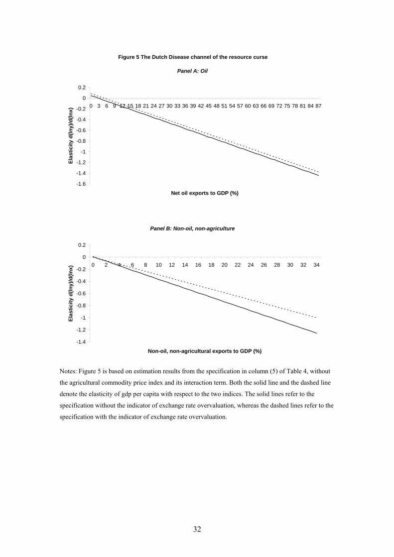
rate indeed has a negative effect on long-run GDP per capita.11 However, the

magnitude of the Dutch disease effect is quite modest. It is depicted in Figure 5 which

shows the effects of oil prices and non-oil, non-agricultural export prices. Each panel

shows two lines. The solid lines denote the interaction effects when we do not control

for exchange rate overvaluation. These effects are based on the specification in

column (5) of Table 4 without the agricultural price index, but applied on a slightly

smaller sample for which we have real exchange rate overvaluation data. The dashed

lines show the interaction effects once we do control for exchange rate overvaluation,

using the same sample. Hence, the differences between the solid and the dashed lines

represent the proportions of the resource curse effects that are due to Dutch Disease.

As can be seen, adding the real exchange rate overvaluation index shifts the lines

upwards, suggesting that part of the negative effects of the export prices works

through the Dutch Disease channel. However, the effect is small: the shift only

captures a small proportion of the total effects.

Volatility

We next investigate the role of volatility. Commodity booms are typically not

permanent and prices tend to show at least some degree of mean reversion over time.

As a result, countries that have experienced one or more commodity export price

boom will typically also have faced higher volatility of export prices. Therefore, it

might be that it is not the commodity booms by themselves that affect long-run GDP

but rather the higher volatility that accompanies them.

The case-study literature on the resource curse points to post-boom crises as being the

key episodes during which growth suffers. To an extent, this can be contrasted with

the Dutch disease effect which hypotheses a continuous rather than episodic reduction

11 To save space, we do not report the results of this regression.

15

in growth rates. We investigate whether the statistical pattern is consistent with an

episodic account of the resource curse. We first divide the observations in our sample

into two groups. The first group, group I, includes the countries for which the non-

agricultural commodity exports to GDP ratio is above the sample median, hence the

“commodity-dependent” countries. The second group, group II, includes the countries

for which the non-agricultural commodity exports to GDP ratio is below the sample

median. The mean growth rate of group II is 0.25 percentage points higher than the

mean growth rate of group I, which is consistent with a resource curse effect. We next

investigate whether this difference in the mean growth rate is due to episodes of

extreme negative growth. We construct two series. For the first series we take the

growth rate of group II and substract the difference between the mean growth rates of

groups I and II (0.25 %). Hence, this series has the mean of group I but the

distribution of group II. The second series equals the growth rates of group I. Hence,

this series has the mean and the distribution of group I. We next construct frequency

distributions for both series and then substract the first series from the second, i.e. we

take the difference between the group I frequency distribution and the group II

frequency distribution. If group I suffers more frequently from negative growth

outliers, this should show in the series. Panel A of Figure 6 shows this difference in

frequency distributions. As can be seen from the left half of the graph, group I does

indeed suffer more frequently from negative growth episodes. We calculate how

much of the difference in the mean growth rates of group I and II can be explained by

these outliers. We define the extreme negative growth outliers as those observations

of log GDP per capita below -3 percentage points (-0.03 on the horizontal axis). We

then multiply the differences in this part of the distribution by the changes in log GDP

per capita (growth) and sum them. The resulting difference in growth is -0.20

percentage points. Hence, of the total difference in mean growth rates of commodity

dependent and non-commodity dependent of 0.25 percentage point, about 0.20

percentage point is explained by negative growth outliers.

These negative outliers only reflect volatility if they correspond to different countries

in individual years rather than to the same countries for several years of persistently

low growth. To distinguish between these two cases, we perform a second procedure.

We first take the mean growth rates of individual countries over time and then divide

the sample again into a group with lower-than-median mean growth and a group with

16

higher-than-median mean growth. We apply the same procedure as before, which

gives us the difference in the frequency distributions of country mean growth rates. If

the negative growth outliers above correspond to several years of persistently low

growth for the same countries, then this should show in the difference between the

frequency distribution of the commodity dependent group of countries and the non-

commodity dependent group of countries. This difference is illustrated in panel B of

Table 6. As can be seen from the graph, commodity dependent countries do not

experience more cases of persistently low growth rates than non-commodity

dependent countries. As a result, we can conclude that the negative outliers above do

in fact reflect volatility rather than persistently low growth ‘disasters’.

However, this does not imply that 80% of the resource curse is explained by volatility.

First, the resource curse is considerably more severe than the 0.25 percentage point

lower growth of the commodity-exporting group of countries, because the

counterfactual should surely be that their favourable resource endowment should be

advantageous rather than simply neutral. Second, it is in one sense unsurprising that

the commodity-exporting countries should have more volatile growth, with high

prices causing booms and low prices causing slumps. The mere fact of severe slumps

does not necessarily indicate that volatility is the problem. It may be entirely

appropriate for a commodity-exporting economy to suffer slumps if by doing so it is

able to harness supra-normal growth during booms. Our accounting exercise is better

seen as a test which might potentially have refuted volatility as an explanation, had

we found that the resource-dependent countries did not suffer more severe slumps.

Governance

There are no long time series on governance, and a formal test of its effects is beyond

the scope of this paper. However, our results do point indirectly to governance as

being critical in the explanation of the resource curse. This is because of the sharp

distinction we have found between the agricultural and non-agricultural commodities.

The export of both agricultural and non-agricultural commodities generates Dutch

disease, and the prices of both are volatile, so neither explanation of the resource

curse would predict this sharp difference. By contrast, it is predicted if governance is

the route through which the resource curse operates.

17

The distinction between agricultural and non-agricultural commodities corresponds to

whether or not the activity generates rents. Agricultural commodities can be produced

in many different locations and so competitive entry will drive profits to normal

levels. The rents on land used for export crops should therefore be no higher than that

used for other crops, once allowance is made for differences in investment, such as

the planting of trees. In contrast, the non-agricultural commodities are all extractive,

the feasibility of production being dependent upon the presence of the resource in the

ground. Hence, the extractive industries all generate rents as a matter of course. Rents

can be taxed without driving the activity away. Thus, whereas the revenues from

agricultural exports accrue as incomes to private factors of production, much of the

revenues from the non-agricultural commodities accrue as rents to government. Here

lies an important potential difference: governance is bound to matter for non-

agricultural commodities because government is directly responsible for spending the

income. Not only is governance intrinsically important, but it is liable to be worse.

For example, both Acemoglu et al. (2002) and Tornell and Lane (1999) propose

routes by which rents from extractive exports would generate a ‘curse’.

5. The Current Commodity Boom: A Simulation

Recently a number of African countries have begun to grow markedly more rapidly

than for the preceding two decades. An important issue is the extent to which this

marks underlying improvements in policies and governance, versus the short term

effects of commodity booms which we have suggested are likely to turn sour. We

therefore apply our estimation results to simulate the effects of the current upturn in

commodity prices on growth in those Sub-Saharan African countries that have

substantial exports of oil or other non-agricultural commodities. We include all

countries for which either oil or other non-agricultural commodity exports to GDP

exceed 5%, a group of 14 countries.12 We construct an oil export price index and an

aggregate index for non-oil, non-agricultural, commodities specific to this group of

countries, using the procedure described previously. Both indices are shown in Figure

7, panel A. Oil prices rose sharply between 1998 and 2000, and increased even more 12 Angola, Cameroon, Democratic Republic of Congo, Republic of Congo, Equatorial Guinea, Gabon, Guinea, Liberia, Mauritania, Namibia, Nigeria, Sudan, Togo, and Zambia.

18

during the period from 2003 until 2006. Non-oil, non-agricultural export prices were

relatively stable before 2003 but also increased sharply between 2003 and 2006.

We next simulate the short-run effects of the commodity boom. In particular, we

rerun the specification in column (5) of Table 4 but without the agricultural

commodity export price index and with separate short-run effects for oil and non-oil,

non-agricultural commodity export prices. We then use the estimated coefficients

from the regression and the log changes in the indices to calculate the short-run

effects on growth. We abstract from the lagged effects of any pre-1999 shocks and

assume that export prices remain at their current levels until 2010. This assumption is

evidently not a forecast, but merely a neutral stance from which to investigate the

likely short and long term consequences of the current boom. Finally, to generate a

counterfactual, we benchmark against the assumption that export prices would have

remained constant at their 1998 levels.

The results are illustrated in Figure 7, panel B. The actual growth rate of this group of

countries has indeed accelerated substantially, as depicted in the panel. Weighted by

GDP, the average per capita growth rate in 2005 was 4.5%, and over the entire post-

1998 period it was 2.29%. How much of this is accounted for by the commodity

boom? The solid line shows the predicted short-run effect of the export price shocks

on growth in the 14 African countries. The two peaks correspond to the two episodes

of price increases in panel A. The effects are substantial. In both 2000 and 2001, as

well as during 2005, 2006, and 2007, the predicted growth effect exceeds 2% points.

The cumulative predicted effect on growth over the same period as actual observed

growth is 1.18%. Hence, our estimate of the underlying growth rate of this group of

economies, abstracting from the commodity boom is 1.1%. This is indeed a little

higher than in previous decades, but it is evidently considerably lower than global

growth and so implies that the tendency for Africa to diverge from the rest of the

world economy has not fundamentally been arrested. On our assumption that global

prices will remain constant at their 2005 level, Africa’s currently high growth rates

persist until 2009 and then collapse. Hence, it may not be until 2010 that it will

become evident whether Africa’s underlying growth has indeed been decisively

raised.

19

Evidently, although the above simulation has applied our model to the issue of short

term growth, the more important implication of the model is for the long term. We

now simulate the long-run effect of the present commodity boom on this group of

countries. Using the aggregate log changes in both price indices between 1999 and

2006, and the aggregate shares of both commodity groups in GDP, our simulation

results suggest that the current commodity boom will in the long run lower per capita

constant-price GDP by 26.0 percent. We should stress that this does not imply a

decline in living standards, since the output decline is mitigated by the direct

contribution of the improved income terms of trade. However, such a major

contraction in output would imply that, far from accelerating, African long term

growth would decelerate.

6. Conclusion

We have found that for non-agricultural commodities, price booms have strong short-

term effects on output, but adverse long-term effects. This has three important

implications. The first is a vindication of the ‘resource curse’ literature. However, we

reject the conventional attribution of the resource curse to Dutch disease: it explains

only a small part of the overall adverse effect. The most likely explanation appears to

be connected with governance. This is an inference from our result that the adverse

effect is confined to the non-agricultural commodities. Whereas agricultural

commodity booms accrue predominantly to farmers, those for non-agricultural

commodities accrue predominantly to government.

The second implication concerns the recent acceleration of growth rates observed in

Africa. Our simulation suggests that around half of current growth in the commodity-

exporting economies is attributable to the short term effects of the commodity boom,

leaving a residual of underlying growth that remains very low.

The final implication is that the current commodity boom is, if past behaviour is

repeated, likely to have strongly adverse long term effects, so that the current

acceleration in growth rates is particularly misleading. However, if our tentative

diagnosis of the root cause of the resource curse as being due to errors in governance

20

is correct, then this dire prognosis may be avoidable. The resource curse would not be

a quasi-mechanistic consequence of a market process such as Dutch disease, but the

result of contingent political processes.

Table 1: Summary Statistics

Obs Mean St dev Min Max

GDP per capita (log) 2418 6.84 1.11 4.31 9.17

Trade to GDP (log) 2405 4.07 0.56 1.84 5.43

External debt to GNI (log) 2416 3.89 0.81 0.12 7.10

CPI (log) 2410 2.60 4.10 -26.84 7.00

M2 to GDP (log) 2416 3.31 0.55 1.41 5.02

CEPI (log) 2220 4.67 0.33 3.27 6.18

Commodity exports to GDP (%) 2418 9.03 8.68 0 44.61

21

OEPI (log) 2418 1.07 1.87 0 4.96

Net oil exports to GDP (%) 2418 3.64 10.68 0 87.86

Oil import price index (log) 2418 3.24 1.88 0 4.96

∆ GDP per capita (log) 2418 0.01 0.05 -0.36 0.30

∆ Trade to GDP (log) 2405 0.01 0.14 -1.20 1.40

∆ External debt to GNI (log) 2416 0.04 0.21 -1.38 1.60

∆ CPI (log) 2410 0.18 0.38 -0.12 5.48

∆ M2 to GDP (log) 2416 0.02 0.13 -1.31 1.53

∆ CEPI (log) 2209 -0.01 0.18 -0.81 1.03

∆ OEPI (log) 2418 0.01 0.13 -0.68 0.93

∆ Oil import price index (log) 2418 0.02 0.22 -0.68 0.93

Coup d’etat 2418 0.03 0.18 0 2

Civil war 2418 0.09 0.29 0 1

Geological shocks 2418 0.05 0.23 0 2

Climatic shocks 2418 0.26 0.51 0 3

Humanitarian shocks 2418 0.02 0.16 0 2

Notes: This table reports summary statistics for all observations used in estimation.

Table 2: List of commodities

Panel A: Non-agricultural commodities

Aluminum Gasoline Natural gas Phosphatrock Uranium

Coal Ironore Nickel Silver Urea

Copper Lead Oil Tin Zinc

Panel B: Agricultural Commodities

Bananas Fish Oliveoil Rice Sunfloweroil

Barley Fishmeal Oranges Rubber Swinemeat

22

Beef Groundnuts Palmkerneloil Shrimp Tea

Butter Groundnutoil Palmoil Sisal Timber

Cocoabeans Hides Pepper Sorghum Tobacco

Coconutoil Jute Potash Soybeans Wheat

Coffee Lamb Poultry Soybeanmeal Wool

Copra Linseedoil Plywood Soybeanoil

Cotton Maize Pulp Sugar

Table 3: Panel unit root and panel cointegration tests

Panel A: Panel unit root tests

Im, Pesaran, Shin (IPS) Maddala and Wu

Levels Differences Levels Differences

GDP per capita (log) -2.31 -4.00*** 75.80 327.47***

Trade to GDP (log) -1.69 -5.97*** 113.83*** 1004.47***

External debt to GNI (log) -1.85** -3.13*** 108.82*** 233.60***

23

CPI (log) -1.47 -1.81** 61.74 92.60**

M2 to GDP (log) -1.63 -2.88*** 52.00 222.87***

CEPI (log) -2.38*** -3.07*** 48.92 249.65***

Dickey-Fuller

Levels Differences

OEPI (log) -2.63* -6.14*** - -

Oil import price index (log) -2.63* -6.14*** - -

Panel B: Pedroni panel cointegration test (based on IPS)

Full sample (unbalanced) Subsample (balanced)

Group t-Statistic -4.70*** -4.52***

Notes: Table 3 reports test statistics for panel unit root and panel cointegration tests. The test statistics

correspond to the t-bar statistic in Im, Pesaran, and Shin (2003), the Fisher χ2 test statistic in Maddala

and Wu (1999), and the statistic Z*t N,T divided by N in Pedroni (1999). The choice of lag order in the

panel unit root tests was based on a pooled (augmented) Dickey-fuller regression with fixed effects,

except for the oil export and import price indices, for which we ran an ordinary (augmented) Dickey-

Fuller test. The number of lags is 1, 0, 2, 4, 2, 4, 0, and 0 for GDP per capita, trade to GDP, external

debt to GNI, CPI, M2 to GDP, CEPI, OEPI, and the oil import price index, respectively. Since equation

(2) includes a time trend, we also include a time trend in the panel unit root test for GDP per capita

(results are similar if we exclude the trend). *, ** denote significance at the 5% and 1% levels,

respectively.

Table 4: Estimation results (1) (2) (3) (4) (5)

Panel A:Estimates of long-run coefficients Trade to GDP (log) 0.342*** 0.352*** 0.355*** 0.359*** 0.362*** (0.104) (0.109) (0.103) (0.104) (0.106) External debt to GNI (log) -0.074** -0.070* -0.018 -0.024 -0.065 (0.036) (0.037) (0.039) (0.040) (0.041) CPI (log) -0.006 -0.005 0.001 0.001 -0.003 (0.006) (0.006) (0.005) (0.005) (0.005) M2 to GDP (log) 0.061 0.082 0.080 0.082 0.064

24

(0.093) (0.097) (0.087) (0.089) (0.098) CEPI (log) -0.144 0.042 (0.199) (0.150) CEPI (log) * Commodity exports to GDP

-0.015** (0.006)

OEPI (log) -0.098 0.049 0.052 (0.087) (0.096) (0.095) OEPI (log) * Net oil exports to GDP

-0.013*** (0.004)

-0.016*** (0.004)

NONA-CEPI (log) -0.030 (0.100) NONA-CEPI (log) * NONA-exports to GDP

-0.035* (0.018)

A-CEPI (log) 0.042 (0.133) A-CEPI (log) * A-exports to GDP

0.012 (0.017)

Oil import price index (log) -0.056 -0.076 -0.108* -0.107* -0.105 (0.062) (0.064) (0.062) (0.062) (0.066) Observations 2169 2169 2418 2418 2169 Number of countries 100 100 115 115 100 R-squared within 0.16 0.16 0.15 0.16 0.17 Notes: The dependent variable is the first-differenced log of real GDP per capita in year t. CEPI is the commodity export price index, OEPI is the oil export price index, NONA-CEPI is the commodity export price index when excluding oil and agricultural commodities. A-CEPI is the commodity export price index when including agricultural commodities only. All regressions include country-specific fixed effects. Robust standard errors are clustered by country and are reported in parentheses. ***, **, and * denote significance at the 1%, 5%, and 10% levels, respectively.

Table 4: Estimation results (cont’d) (1) (2) (3) (4) (5)

Panel B: Estimate of short-run adjustment coefficients GDP per capita (log)t-1 -0.065*** -0.064*** -0.060*** -0.059*** -0.064*** (0.010) (0.009) (0.008) (0.008) (0.009)

Panel C: Estimates of short-run coefficients: commodity prices, oil prices, and GDP ∆ (CEPI (log))t 0.016** 0.016** 0.017** (0.008) (0.008) (0.008) ∆ (CEPI (log))t-1 0.027*** 0.025*** 0.023***

25

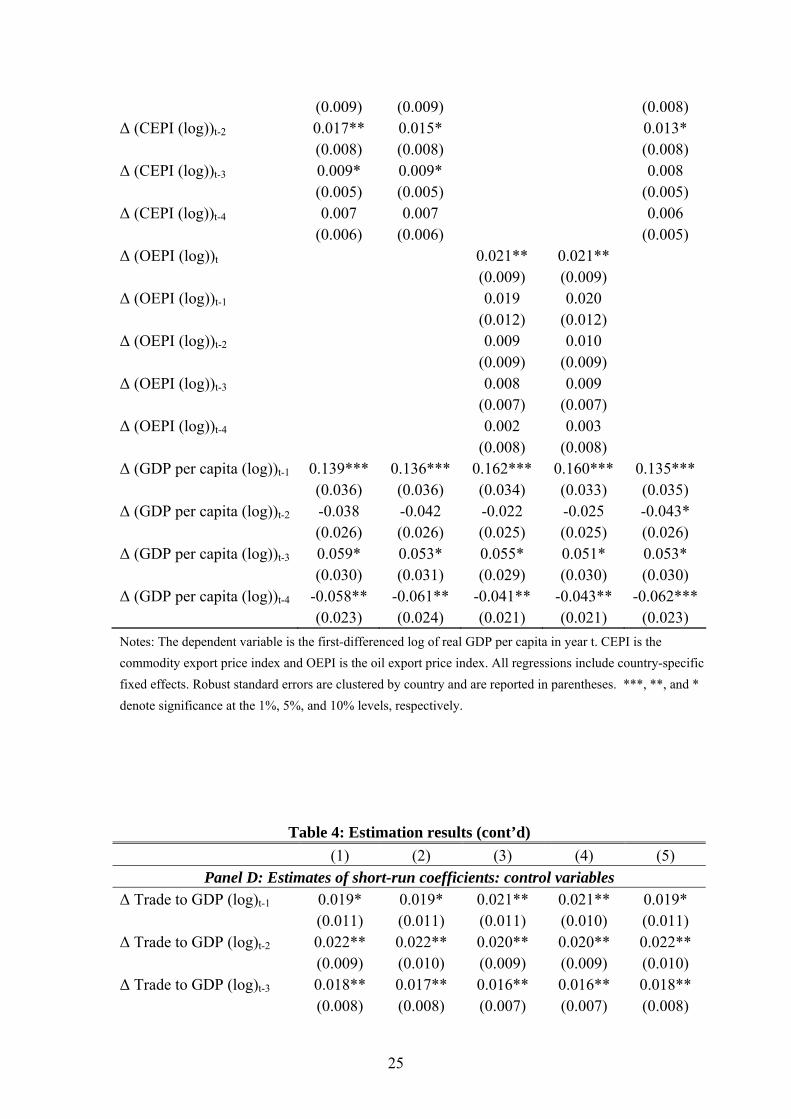
(0.009) (0.009) (0.008) ∆ (CEPI (log))t-2 0.017** 0.015* 0.013* (0.008) (0.008) (0.008) ∆ (CEPI (log))t-3 0.009* 0.009* 0.008 (0.005) (0.005) (0.005) ∆ (CEPI (log))t-4 0.007 0.007 0.006 (0.006) (0.006) (0.005) ∆ (OEPI (log))t 0.021** 0.021** (0.009) (0.009) ∆ (OEPI (log))t-1 0.019 0.020 (0.012) (0.012) ∆ (OEPI (log))t-2 0.009 0.010 (0.009) (0.009) ∆ (OEPI (log))t-3 0.008 0.009 (0.007) (0.007) ∆ (OEPI (log))t-4 0.002 0.003 (0.008) (0.008) ∆ (GDP per capita (log))t-1 0.139*** 0.136*** 0.162*** 0.160*** 0.135*** (0.036) (0.036) (0.034) (0.033) (0.035) ∆ (GDP per capita (log))t-2 -0.038 -0.042 -0.022 -0.025 -0.043* (0.026) (0.026) (0.025) (0.025) (0.026) ∆ (GDP per capita (log))t-3 0.059* 0.053* 0.055* 0.051* 0.053* (0.030) (0.031) (0.029) (0.030) (0.030) ∆ (GDP per capita (log))t-4 -0.058** -0.061** -0.041** -0.043** -0.062*** (0.023) (0.024) (0.021) (0.021) (0.023) Notes: The dependent variable is the first-differenced log of real GDP per capita in year t. CEPI is the commodity export price index and OEPI is the oil export price index. All regressions include country-specific fixed effects. Robust standard errors are clustered by country and are reported in parentheses. ***, **, and * denote significance at the 1%, 5%, and 10% levels, respectively.

Table 4: Estimation results (cont’d) (1) (2) (3) (4) (5) Panel D: Estimates of short-run coefficients: control variables

∆ Trade to GDP (log)t-1 0.019* 0.019* 0.021** 0.021** 0.019* (0.011) (0.011) (0.011) (0.010) (0.011) ∆ Trade to GDP (log)t-2 0.022** 0.022** 0.020** 0.020** 0.022** (0.009) (0.010) (0.009) (0.009) (0.010) ∆ Trade to GDP (log)t-3 0.018** 0.017** 0.016** 0.016** 0.018** (0.008) (0.008) (0.007) (0.007) (0.008)

26

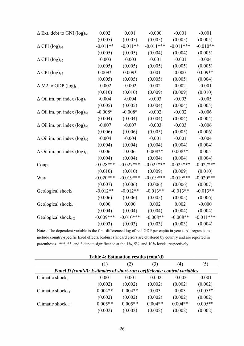
∆ Ext. debt to GNI (log)t-1 0.002 0.001 -0.000 -0.001 -0.001 (0.005) (0.005) (0.005) (0.005) (0.005) ∆ CPI (log)t-1 -0.011** -0.011** -0.011*** -0.011*** -0.010** (0.005) (0.005) (0.004) (0.004) (0.005) ∆ CPI (log)t-2 -0.003 -0.003 -0.001 -0.001 -0.004 (0.005) (0.005) (0.005) (0.005) (0.005) ∆ CPI (log)t-3 0.009* 0.009* 0.001 0.000 0.009** (0.005) (0.005) (0.005) (0.005) (0.004) ∆ M2 to GDP (log)t-1 -0.002 -0.002 0.002 0.002 -0.001 (0.010) (0.010) (0.009) (0.009) (0.010) ∆ Oil im. pr. index (log)t -0.004 -0.004 -0.003 -0.003 -0.005 (0.005) (0.005) (0.004) (0.004) (0.005) ∆ Oil im. pr. index (log)t-1 -0.008* -0.008* -0.002 -0.002 -0.006 (0.004) (0.004) (0.004) (0.004) (0.004) ∆ Oil im. pr. index (log)t-2 -0.007 -0.007 -0.003 -0.003 -0.006 (0.006) (0.006) (0.005) (0.005) (0.006) ∆ Oil im. pr. index (log)t-3 -0.004 -0.004 -0.001 -0.001 -0.004 (0.004) (0.004) (0.004) (0.004) (0.004) ∆ Oil im. pr. index (log)t-4 0.006 0.006 0.008** 0.008** 0.005 (0.004) (0.004) (0.004) (0.004) (0.004) Coupt -0.028*** -0.027*** -0.025*** -0.025*** -0.027*** (0.010) (0.010) (0.009) (0.009) (0.010) Wart -0.020*** -0.019*** -0.019*** -0.019*** -0.020*** (0.007) (0.006) (0.006) (0.006) (0.007) Geological shockt -0.012** -0.012** -0.013** -0.013** -0.013** (0.006) (0.006) (0.005) (0.005) (0.006) Geological shockt-1 0.000 0.000 0.002 0.002 -0.000 (0.004) (0.004) (0.004) (0.004) (0.004) Geological shockt-2 -0.009*** -0.010*** -0.008** -0.008** -0.011*** (0.003) (0.003) (0.003) (0.003) (0.004) Notes: The dependent variable is the first-differenced log of real GDP per capita in year t. All regressions include country-specific fixed effects. Robust standard errors are clustered by country and are reported in parentheses. ***, **, and * denote significance at the 1%, 5%, and 10% levels, respectively.

Table 4: Estimation results (cont’d) (1) (2) (3) (4) (5)

Panel D (cont’d): Estimates of short-run coefficients: control variables Climatic shockt -0.001 -0.001 -0.002 -0.002 -0.001 (0.002) (0.002) (0.002) (0.002) (0.002) Climatic shockt-1 0.004** 0.004** 0.003 0.003 0.005** (0.002) (0.002) (0.002) (0.002) (0.002) Climatic shockt-2 0.005** 0.005** 0.004** 0.004** 0.005** (0.002) (0.002) (0.002) (0.002) (0.002)

27

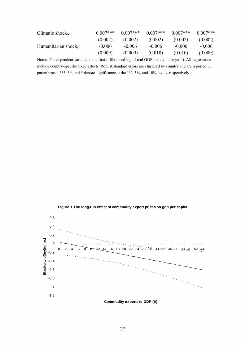
Climatic shockt-3 0.007*** 0.007*** 0.007*** 0.007*** 0.007*** (0.002) (0.002) (0.002) (0.002) (0.002) Humanitarian shockt -0.006 -0.006 -0.006 -0.006 -0.006 (0.009) (0.009) (0.010) (0.010) (0.009) Notes: The dependent variable is the first-differenced log of real GDP per capita in year t. All regressions include country-specific fixed effects. Robust standard errors are clustered by country and are reported in parentheses. ***, **, and * denote significance at the 1%, 5%, and 10% levels, respectively.

Figure 1 The long-run effect of commodity export prices on gdp per capita

-1.2

-1

-0.8

-0.6

-0.4

-0.2

0

0.2

0.4

0.6

0 2 4 6 8 10 12 14 16 18 20 22 24 26 28 30 32 34 36 38 40 42 44

Commodity exports to GDP (%)

Elas

ticity

d(ln

y)/d

(lnx)

28

Notes: Figure 1 is based on the estimation results in panel A of Table 4 (column (2)). The solid line

denotes the elasticity of gdp per capita with respect to commodity export prices. The dashed lines

illustrate the 95% confidence interval. The range of values on the horizontal axis corresponds to the

range of values in our sample.

29

Figure 2 The long-run effect of oil, non-oil non-agricultural, and agricultural commodity export prices on gdp per capita

Panel A: Oil

-2.5

-2

-1.5

-1

-0.5

0

0.5

0 3 6 9 12 15 18 21 24 27 30 33 36 39 42 45 48 51 54 57 60 63 66 69 72 75 78 81 84 87

Net oil exports to GDP (%)

Elas

ticity

d(ln

y)/d

(lnx)

Panel B: Non-oil, non-agriculture

-2.5

-2

-1.5

-1

-0.5

0

0.5

0 2 4 6 8 10 12 14 16 18 20 22 24 26 28 30 32 34

Non-oil, non-agricultural exports to GDP (%)

Elas

ticity

d(ln

y)/d

(lnx)

Panel C: Agriculture

-0.6

-0.4

-0.2

0

0.2

0.4

0.6

0.8

1

1.2

0 1 2 3 4 5 6 7 8 9 10 11 12 13 14 15 16 17 18 19 20 21 22 23 24

Agricultural exports to GDP (%)

Elas

ticity

d(ln

y)/d

(lnx)

Notes: Figure 2 is based on the estimation results in panel A of Table 4 (column (5)). The solid line denotes the elasticity of gdp per capita with respect to the three indices. The dashed lines illustrate the 95% confidence interval. The range of values on the horizontal axes corresponds to the range of values in our sample.

30

Figure 3 The short-run effect of commodity export prices on gdp per capita

-0.04

-0.03

-0.02

-0.01

0

0.01

0.02

0.03

0.04

t t+1 t+2 t+3 t+4

period

effe

ct o

n gr

owth

d(d

.lny)

/d(d

.lnx)

Notes: Figure 3 is based on the estimation results in panel C of Table 4 (column (1)). The solid line

denotes the impulse response function of a shock to the commodity export price index in period t. A

value of 0.015 on the vertical axis implies that a 10 percentage point increase in the growth rate of

commodity export prices leads to a 0.15 percentage point increase in the gdp per capita growth rate.

The dashed lines illustrate the 95% confidence interval.

31

Figure 4 The short-run effect of oil export prices on gdp per capita

-0.04

-0.03

-0.02

-0.01

0

0.01

0.02

0.03

0.04

0.05

t t+1 t+2 t+3 t+4

period

effe

ct o

n gr

owth

d(d

.lny)

/d(d

.lnx)

Notes: Figure 4 is based on the estimation results in panel C of Table 4 (column (3)). The solid line

denotes the impulse response function of a shock to the oil export price index in period t. A value of

0.02 on the vertical axis implies that a 10 percentage point increase in the growth rate of oil export

prices leads to a 0.20 percentage point increase in the gdp per capita growth rate. The dashed lines

illustrate the 95% confidence interval.

32

Figure 5 The Dutch Disease channel of the resource curse

Panel A: Oil

-1.6

-1.4

-1.2

-1

-0.8

-0.6

-0.4

-0.2

0

0.2

0 3 6 9 12 15 18 21 24 27 30 33 36 39 42 45 48 51 54 57 60 63 66 69 72 75 78 81 84 87

Net oil exports to GDP (%)

Elas

ticity

d(ln

y)/d

(lnx)

Panel B: Non-oil, non-agriculture

-1.4

-1.2

-1

-0.8

-0.6

-0.4

-0.2

0

0.2

0 2 4 6 8 10 12 14 16 18 20 22 24 26 28 30 32 34

Non-oil, non-agricultural exports to GDP (%)

Elas

ticity

d(ln

y)/d

(lnx)

Notes: Figure 5 is based on estimation results from the specification in column (5) of Table 4, without

the agricultural commodity price index and its interaction term. Both the solid line and the dashed line

denote the elasticity of gdp per capita with respect to the two indices. The solid lines refer to the

specification without the indicator of exchange rate overvaluation, whereas the dashed lines refer to the

specification with the indicator of exchange rate overvaluation.

33

Figure 6: The volatility channel of the resource curse

Panel A: All country-year growth observations

-0.03

-0.02

-0.01

0.00

0.01

0.02

-0.39 -0.33 -0.27 -0.21 -0.15 -0.09 -0.03 0.03 0.09 0.15 0.21 0.27 0.33 0.39

change in log GDP per capita

diffe

renc

e in

fr

eque

ncy

dist

ribut

ions

Panel B: Mean country growth observations only

-0.1

-0.05

0

0.05

0.1

0.15

-0.08 -0.07 -0.05 -0.04 -0.03 -0.02 -0.01 0.01 0.02 0.03 0.04 0.05 0.07 0.08

change in log GDP per capita

diffe

renc

e in

freq

uenc

y di

strib

utio

ns

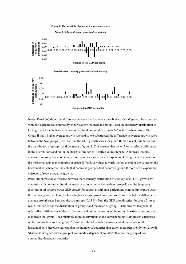
Notes: Panel (A) shows the difference between the frequency distribution of GDP growth for countries

with non-agricultural commodity exports above the median (group I) and the frequency distribution of

GDP growth for countries with non-agricultural commodity exports below the median (group II).

Group II has a higher average growth rate and so we substracted the difference in average growth rates

between the two groups (0.25 %) from the GDP growth series for group II. As a result, this series has

the distribution of group II and the mean of group I. This ensures that panel A only reflects differences

in the distributions and not in the means of the series. Positive values in panel A indicate that the

countries in group I have relatively more observations in the corresponding GDP growth categories on

the horizontal axis than countries in group II. Positive values towards the lower end of the values on the

horizontal axis therefore indicate that commodity-dependent countries (group I) more often experience

episodes of severe negative growth. Panel (B) shows the difference between the frequency distribution of country mean GDP growth for

countries with non-agricultural commodity exports above the median (group 1) and the frequency

distribution of country mean GDP growth for countries with non-agricultural commodity exports below

the median (group 2). Group 2 has a higher average growth rate and so we substracted the difference in

average growth rates between the two groups (0.15 %) from the GDP growth series for group 2. As a

result, this series has the distribution of group 2 and the mean of group 1. This ensures that panel B

only reflects differences in the distributions and not in the means of the series. Positive values in panel

B indicate that group 1 has relatively more observations in the corresponding GDP growth categories

on the horizontal axis than group 2. Positive values towards the lower end of the values on the

horizontal axis therefore indicate that the number of countries that experiences persistently low growth

‘disasters’ is higher for the group of commodity-dependent countries than for the group of non

commodity-dependent countries.

34

Panel B: Predicted effects on growth (solid line) and actual growth rates (dashed line)

-1

0

1

2

3

4

5

1999 2000 2001 2002 2003 2004 2005 2006 2007 2008 2009 2010

year

effe

ct o

n gr

owth

(% p

oint

s)

Figure 7: A simulation of the short-run effects of the current commodity boom on growth in Africa's commodity exporting

countries

Panel A: Export price indices

0

50

100

150

200

250

1996 1998 2000 2002 2004 2006

year

inde

x (2

000=

100)

non-oil, non-agricultureoil

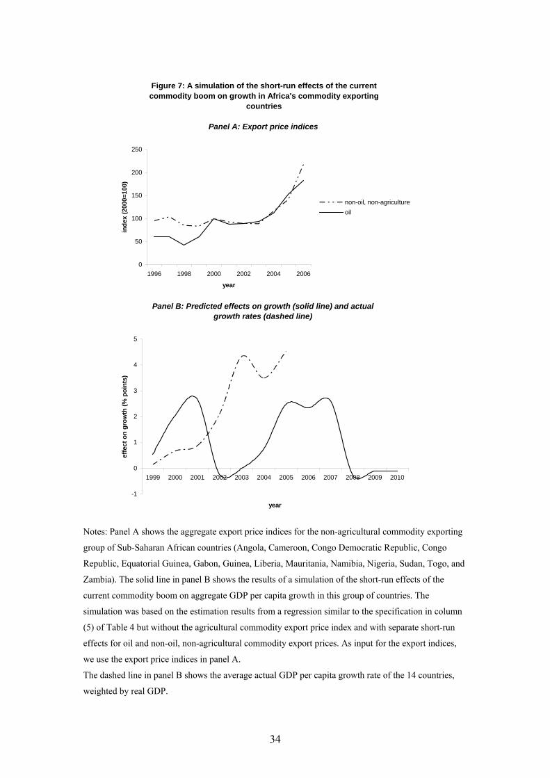
Notes: Panel A shows the aggregate export price indices for the non-agricultural commodity exporting

group of Sub-Saharan African countries (Angola, Cameroon, Congo Democratic Republic, Congo

Republic, Equatorial Guinea, Gabon, Guinea, Liberia, Mauritania, Namibia, Nigeria, Sudan, Togo, and

Zambia). The solid line in panel B shows the results of a simulation of the short-run effects of the

current commodity boom on aggregate GDP per capita growth in this group of countries. The

simulation was based on the estimation results from a regression similar to the specification in column

(5) of Table 4 but without the agricultural commodity export price index and with separate short-run

effects for oil and non-oil, non-agricultural commodity export prices. As input for the export indices,

we use the export price indices in panel A.

The dashed line in panel B shows the average actual GDP per capita growth rate of the 14 countries,

weighted by real GDP.

35

References Acemoglu, D., Johnson, S. and Robinson, J.A. (2001). ‘The colonial origins of

comparative development: An empirical investigation’, American Economic

Review, Vol. 91, pp. 1369-1401.

Auty, R. M. (2001). Resource Abundance and Economic Development, Oxford

University Press, Oxford. Bravo-Ortega, C. and De Gregorio, J. (2001). ‘The relative richness of the poor?

Natural resources, human capital, and economic growth, mimeo University of

California, Berkeley.

Collier, P. (1999). ‘On the economic consequences of civil war’, Oxford Economic

Papers, Vol. 51, pp. 168-83.

Corden, W. M. and Neary, J. P. (1982). ‘Booming sector and de-industrialization in a

small open economy’, Economic Journal, Vol. 92, pp. 825-848.

Deaton, A. and Miller, R. (1996). ‘International commodity prices, macroeconomic

performance and politics in Sub-Saharan Africa’, Journal of African Economies,

Vol. 5, pp. 99-191.

Dehn, J. (2000). ‘Commodity price uncertainty in developing countries’, CSAE

Working Paper 2000-12.

Im, K.S., Pesaran, M.H. and Shin, Y. (2003). ‘Testing for unit roots in heterogenous

panels’, Journal of Econometrics, Vol. 115, pp. 53-74.

Lane, P. R. and Tornell, A. (1996). ‘Power, growth and the voracity effect’, Journal

of Economic Growth, Vol. 1, pp. 213–41.

Leite, C., and Weidmann, M. (1999). ‘Does mother nature corrupt? Natural resources,

corruption, and economic growth’, IMF Working Paper 99/85.

Levin, A., Lin, C.-F. and Chu, C.-S.J. (2002). ‘Unit root tests in panel data:

Asymptotic and finite sample properties’, Journal of Econometrics, Vol. 108, pp. 1-

24.

Maddala, G.S. and Wu, S. (1999). ‘A comparative study of unit root tests with panel

data and a new simple test’, Oxford Bulletin of Economics and Statistics, Vol. 61,

pp. 631-652.

Pedroni, P. (1999). ‘Critical values for cointegration tests in heterogenous panels with

multiple regressors’, Oxford Bulletin of Economics and Statistics, Vol. 61, pp. 653-

670.

36

Raddatz, C. (2005). ‘Are external shocks responsible for the instability of output in

low-income countries?’, World Bank Policy Research Working Paper 3680.

Sachs, J. D. and Warner, A. M. (1995). ‘Natural resource abundance and economic

growth’, NBER Working Paper 5398.

Sachs, J. D. and Warner, A. M. (1997a). ‘Natural resource abundance and economic

growth – revised version’, Working Paper, Harvard University.

Sachs, J. D. and Warner, A. M. (1997b). ‘Sources of slow growth in African

economies’, Journal of African Economies, Vol. 6, pp. 335–76.

Sala-i-Martin, X. and Subramanian, A. (2003). ‘Addressing the natural resource

curse: An illustration from Nigeria’, IMF Working Paper 03/139.

Tornell, A. and Lane, P.R. (1999). ‘The voracity effect’, American Economic Review,

Vol. 89, pp. 22–46.

Torvik, R. (2002). ‘Natural resources, rent seeking and welfare’, Journal of

Development Economics, Vol. 67, pp. 455–70.

Van Wijnbergen, S. J. G. (1984). ‘The Dutch disease: a disease after all?’, Economic

Journal, Vol. 94, pp. 41-55.

37

Appendix This appendix provides the data sources for the variables used in estimation.

Real GDP per capita

GDP per capita in constant 2000 US dollars, taken from the World Development

Indicators.

Commodity export price index

Commodity export values for 1990 are from the UNCTAD Commodity Yearbook

2000 and the United Nations International Trade Statistics 1993 and 1994. Quarterly

world commodity price indices are taken from the IMF’s International Financial

Statistics (series 76, except for butter and coal where we use series 74). Four

commodity price series (coal, plywood, silver, and sorghum) had several short gaps in

the early sample periods. Following Dehn (2000), we filled these gaps by holding the

price constant at the value of the first available observation. Four price series

(palmkerneloil, bananas, tobacco, and silver) had 1, 2, or 3 missing quarterly values

in the middle of the series. Again following Dehn (2000) these gaps were filled by

linear interpolation. Price series with larger gaps were not adjusted. However, where

gaps would cause missing export price index observations in countries for which this

commodity was relatively unimportant (share of exports in total commodity exports

smaller than 10%), these price series were left out of the index.

The geometrically weighted commodity export price index was first calculated on a

quarterly basis and deflated by the export unit value, taken from the IMF’s

International Financial Statistics (series 74..DZF). We then calculated the annual

averages.

Commodity exports to GDP (%)

Commodity export values for 1990 are from the UNCTAD Commodity Yearbook

2000 and the United Nations International Trade Statistics 1993 and 1994. GDP is in

current US dollars for 1990, taken from the World Development Indicators.

Oil import price index and oil export price index

38

The index of world oil prices was taken from the IMF’s International Financial

Statistics (series 00176AADZF) and is a spot price index of the average world price

of crude petroleum. The dummy variables for net oil importing and net oil exporting

countries are based on net oil imports in 2001. We defined net oil imports as crude oil

imports plus total imports of refined petroleum products minus crude oil exports

minus total exports of refined petroleum products, all taken from the Energy

Information Administration’s International Energy Annual 2002. Since these

components are expressed in thousands of barrels per day, we multiplied them by 365

times the 2001 average weekly world oil price per barrel, also taken from the Energy

Information Administration. If net oil imports are positive, the dummy for net oil

importing countries is 1, otherwise it is zero. If net oil imports are negative, the

dummy for net oil exporting countries is 1, otherwise it is zero.

Net oil exports to GDP (%)

Net oil exports are defined as minus net oil imports, where net oil imports consist of

net crude oil imports plus net imports of refined petroleum products, all taken from

the Energy Information Administration’s International Energy Annual 2002 and

expressed in current US dollars using the procedure described under the previous

item. GDP is in current US dollars for 2001, taken from the World Development

Indicators.

Trade openness

Trade (% of GDP): the sum of exports and imports of goods and services measured as

a share of GDP, taken from the World Development Indicators.

External debt

Total external debt to gross national product, taken from Global Development Finance.

Inflation

Consumer price index (2000=100), taken from World Development Indicators.

Financial development

39

Money and quasi money (M2) as % of GDP, taken from World Development

Indicators.

Civil war

Dummy variable: 1 for civil war, 0 otherwise, taken from Gleditsch (2004) and

available at http://weber.ucsd.edu/~kgledits/expwar.html.

Coup d’etat

The number of extraconstitutional or forced changes in the top government elite

and/or its effective control of the nation's power structure in a given year, taken from

Banks' Cross-National Time-Series Data Archive and available at

http://www.scc.rutgers.edu/cnts/about.cfm. Unsuccessful coups are not counted.

Geological, climatic, and human disasters

Geological disasters include earthquakes, landslides, volcano eruptions, and tidal

waves. Climatic disasters include floods, droughts, extreme temperatures, and wind

storms. Human disasters include famines and epidemics. In order to identify disasters

that could affect a country’s macroeconomic performance, we construct each of the

three variables as the annual number of episodes that qualify as large disasters

according to the criteria established by the International Monetary Fund (IMF, 2003).

A large disaster affects at least 0.5% of the population, or causes damage of at least

0.5% of GDP, or causes at least 1 death per 10000 people. Data are taken from the

WHO Collaborating Centre for Research on the Epidemiology of Disasters (CRED)

and are available at www.em-dat.net.

UNCTAD commodity price index

Commodity price index that includes a wide range of commodities: (i) food and

tropical beverages, (ii) vegetable oilseeds and oils, (iii) agricultural raw materials, and

(iv) ores, minerals, and metals (source: Commodity Price Statistics, United Nations

Conference on Trade and Development (UNCTAD)). The index was first deflated by

the export unit value, taken from the IMF’s International Financial Statistics (series

74..DZF). Then we constructed the annual averages of the monthly deflated index.

UNCTAD oil price index

40

Crude petroleum index based on the average of Dubai, United Kingdom Brent and

West Texas Intermediate crude prices, reflecting relatively equal consumption of

medium, light and heavy crudes worldwide. (source: Commodity Price Statistics,

United Nations Conference on Trade and Development (UNCTAD)). The index was

first deflated by the export unit value, taken from the IMF’s International Financial

Statistics (series 74..DZF). Then we constructed the annual averages of the monthly

deflated index.