Embed Size (px)
Citation preview

Incomplete markets with Real Assets
COMMODITIES: INCOMPLETE MARKETS
Roger J-B Wets
PIMS, . . . Managing Risk, Natural Resources
Vancouver, B.C. - July 2008

Incomplete markets with Real Assets
Collaborators & Contributors
⋆ Alejandro Jofré, Universidad de Chile⋆ R.T. Rockafellar, University of Washington
Computational project:⋆ Michael Ferris, University of Wisconsin⋆ Julio Deride, Universidad de Chile
- Comments: William Zame, Martine Quinzii, Jacques Drèze,Kenneth Arrow, Yves Balasko, Roger Guesnerie, MoniqueFlorenzano, Ivar Ekeland, Michel Grandmont, ...
Incomplete markets with Real Assets
Outline
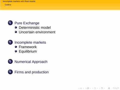
1 Pure ExchangeDeterministic modelUncertain environment
2 Incomplete marketsFrameworkEquilibrium
3 Numerical Approach
4 Firms and production
Incomplete markets with Real Assets
Outline
1 Pure ExchangeDeterministic modelUncertain environment
2 Incomplete marketsFrameworkEquilibrium
3 Numerical Approach
4 Firms and production
Incomplete markets with Real Assets
Outline
1 Pure ExchangeDeterministic modelUncertain environment
2 Incomplete marketsFrameworkEquilibrium
3 Numerical Approach
4 Firms and production
Incomplete markets with Real Assets
Outline
1 Pure ExchangeDeterministic modelUncertain environment
2 Incomplete marketsFrameworkEquilibrium
3 Numerical Approach
4 Firms and production
Incomplete markets with Real Assets
Pure Exchange
Deterministic model
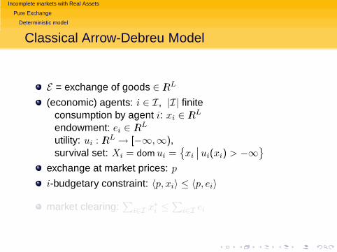
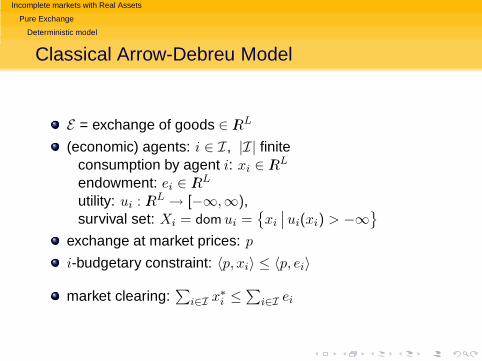
Classical Arrow-Debreu Model
E = exchange of goods ∈ IRL
(economic) agents: i ∈ I, |I| finiteconsumption by agent i: xi ∈ IRL
endowment: ei ∈ IRL
utility: ui : IRL → [−∞,∞),survival set: Xi = dom ui =
{
xi
∣
∣ui(xi) > −∞}
exchange at market prices: p
i-budgetary constraint: 〈p, xi〉 ≤ 〈p, ei〉
market clearing:∑
i∈I x∗i ≤
∑
i∈I ei
Incomplete markets with Real Assets
Pure Exchange
Deterministic model
Classical Arrow-Debreu Model
E = exchange of goods ∈ IRL
(economic) agents: i ∈ I, |I| finiteconsumption by agent i: xi ∈ IRL
endowment: ei ∈ IRL
utility: ui : IRL → [−∞,∞),survival set: Xi = dom ui =
{
xi
∣
∣ui(xi) > −∞}
exchange at market prices: p
i-budgetary constraint: 〈p, xi〉 ≤ 〈p, ei〉
market clearing:∑
i∈I x∗i ≤
∑
i∈I ei
Incomplete markets with Real Assets
Pure Exchange
Uncertain environment
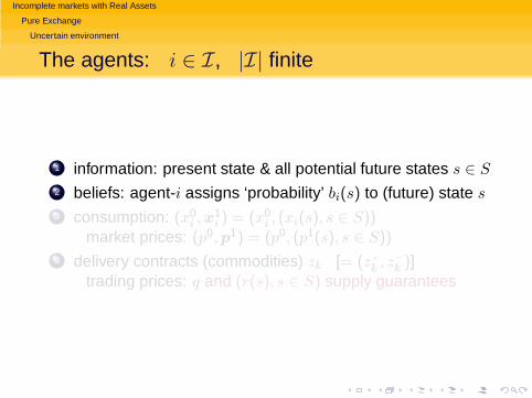
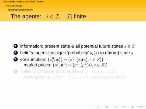
The agents: i ∈ I, |I| finite
1 information: present state & all potential future states s ∈ S
2 beliefs: agent-i assigns ‘probability’ bi(s) to (future) state s
3 consumption: (x0i ,x
1i ) = (x0
i , (xi(s), s ∈ S))market prices: (p0,p1) = (p0, (p1(s), s ∈ S))
4 delivery contracts (commodities) zk [= (z+
k , z−
k )]trading prices: q and (r(s), s ∈ S) supply guarantees
Incomplete markets with Real Assets
Pure Exchange
Uncertain environment
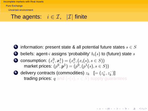
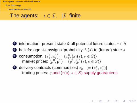
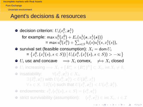
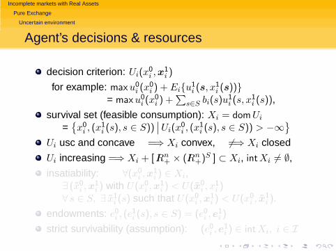
Agent’s decisions & resources
decision criterion: Ui(x0i ,x
1i )
for example: maxu0i (x
0i ) + Ei{u
1i (s, x1
i (s))}= maxu0
i (x0i ) +
∑
s∈S bi(s)u1i (s, x
1i (s)),
survival set (feasible consumption): Xi = domUi
={
x0i , (x
1i (s), s ∈ S))
∣
∣ Ui(x0i , (x
1i (s), s ∈ S)) > −∞
}
Ui usc and concave =⇒ Xi convex, 6=⇒ Xi closed
Ui increasing =⇒ Xi + [ IRn+ × (IRn
+)S ] ⊂ Xi, intXi 6= ∅,
insatiability: ∀(x0i ,x
1i ) ∈ Xi,
∃ (x̃0i ,x
1i ) with U(x0
i ,x1i ) < U(x̃0
i , x1i )
∀ s ∈ S, ∃ x̃1i (s) such that U(x0
i ,x1i ) < U(x0
i , x̃1i ).
endowments: e0i , (e
1i (s), s ∈ S) = (e0
i ,e1i )
strict survivability (assumption): (e0i ,e
1i ) ∈ intXi, i ∈ I
Incomplete markets with Real Assets
Pure Exchange
Uncertain environment
Agent’s decisions & resources
decision criterion: Ui(x0i ,x
1i )
for example: maxu0i (x
0i ) + Ei{u
1i (s, x1
i (s))}= maxu0
i (x0i ) +
∑
s∈S bi(s)u1i (s, x
1i (s)),
survival set (feasible consumption): Xi = domUi
={
x0i , (x
1i (s), s ∈ S))
∣
∣ Ui(x0i , (x
1i (s), s ∈ S)) > −∞
}
Ui usc and concave =⇒ Xi convex, 6=⇒ Xi closed
Ui increasing =⇒ Xi + [ IRn+ × (IRn
+)S ] ⊂ Xi, intXi 6= ∅,
insatiability: ∀(x0i ,x
1i ) ∈ Xi,
∃ (x̃0i ,x
1i ) with U(x0
i ,x1i ) < U(x̃0
i , x1i )
∀ s ∈ S, ∃ x̃1i (s) such that U(x0
i ,x1i ) < U(x0
i , x̃1i ).
endowments: e0i , (e
1i (s), s ∈ S) = (e0
i ,e1i )
strict survivability (assumption): (e0i ,e
1i ) ∈ intXi, i ∈ I

Incomplete markets with Real Assets
Pure Exchange
Uncertain environment
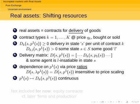
Real assets: Shifting resources
1 real assets = contracts for delivery of goods2 contract types k = 1, . . . ,K @ price qk, bought or sold3 Dk(s, p
1(s)) ≥ 0 delivery in state ‘s’ per unit of contract kDk,l(s, p
1(s)) > 0 some state s ∈ S some good ‘l’4 Delivery matrix: D(s, p1(s)) = [ · · ·Dk(s, p1(s)) · · · ]
& some agent is l-insatiable in state s
5 dependence on p1(s) via price ratiosD(s, λp1(s)) = D(s, p1(s)) insensitive to price scaling
6 p1(s) 7→ Dk(s, p1(s)) continuous
Not included for now: equity contractscf. later ‘firms and production’
Incomplete markets with Real Assets
Pure Exchange
Uncertain environment
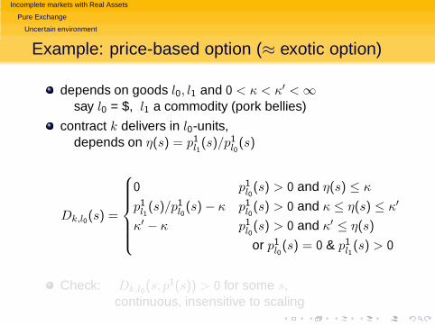
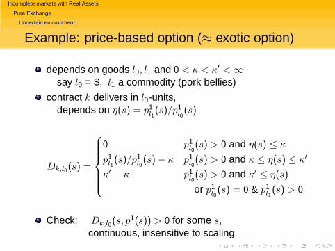
Example: price-based option (≈ exotic option)
depends on goods l0, l1 and 0 < κ < κ′ < ∞say l0 = $, l1 a commodity (pork bellies)
contract k delivers in l0-units,depends on η(s) = p1
l1(s)/p1
l0(s)
Dk,l0(s) =
0 p1l0(s) > 0 and η(s) ≤ κ
p1l1(s)/p1
l0(s) − κ p1
l0(s) > 0 and κ ≤ η(s) ≤ κ′
κ′ − κ p1l0(s) > 0 and κ′ ≤ η(s)
or p1l0(s) = 0 & p1
l1(s) > 0
Check: Dk,l0(s, p1(s)) > 0 for some s,
continuous, insensitive to scaling
Incomplete markets with Real Assets
Pure Exchange
Uncertain environment
Example: price-based option (≈ exotic option)
depends on goods l0, l1 and 0 < κ < κ′ < ∞say l0 = $, l1 a commodity (pork bellies)
contract k delivers in l0-units,depends on η(s) = p1
l1(s)/p1
l0(s)
Dk,l0(s) =
0 p1l0(s) > 0 and η(s) ≤ κ
p1l1(s)/p1
l0(s) − κ p1
l0(s) > 0 and κ ≤ η(s) ≤ κ′
κ′ − κ p1l0(s) > 0 and κ′ ≤ η(s)
or p1l0(s) = 0 & p1
l1(s) > 0
Check: Dk,l0(s, p1(s)) > 0 for some s,
continuous, insensitive to scaling
Incomplete markets with Real Assets
Incomplete markets
Framework
Contracts and deliveries
z+
i contract purchases and z−
i sales of agent-i
simultaneous buying/selling allowedbut won’t occur! cf. assumptions: Dk,l(s, p
1(s))
(z+
i , z−
i ) generates D(s, p1(s))[z+
i − z−
i ] goods
time 0: cost 〈q, z+
i − z−
i 〉
time 1: value 〈p1(s),D(s, p1(s))[z+
i − z−
i ]〉
.
Vk(s, p1)=〈p1,Dk(s, p
1), Vk(p1)〉=(. . . Vk(s, p
1) . . . ) ∈ IR|S|
V (p1) = [ |S| × K ]-matrix
W (p1) = linV (p1), linear span of {Vk(s, p1)}
Financial market is complete for p1 if W (p1) = IR|S|
∀ t ∈ IR|S|,∃ portfolio: V (p1)[z+ − z−] = t

Incomplete markets with Real Assets
Incomplete markets
Framework
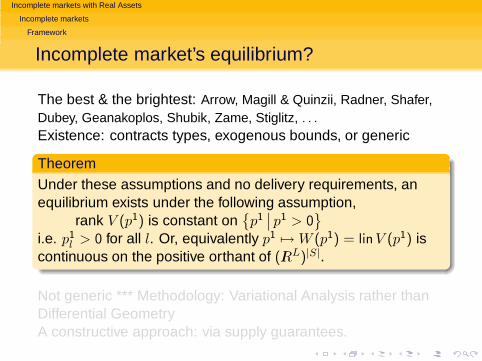
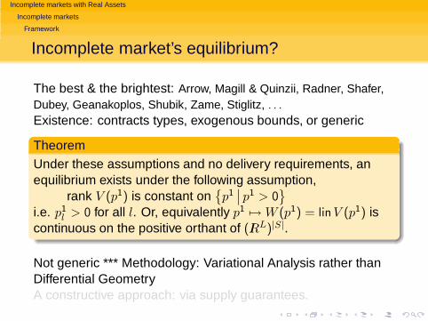
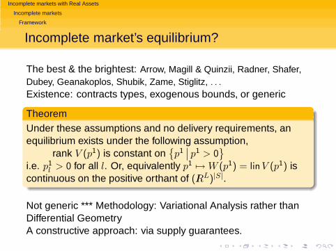
Incomplete market’s equilibrium?
The best & the brightest: Arrow, Magill & Quinzii, Radner, Shafer,Dubey, Geanakoplos, Shubik, Zame, Stiglitz, . . .
Existence: contracts types, exogenous bounds, or generic
TheoremUnder these assumptions and no delivery requirements, anequilibrium exists under the following assumption,
rank V (p1) is constant on{
p1∣
∣ p1 > 0}
i.e. p1l > 0 for all l. Or, equivalently p1 7→ W (p1) = linV (p1) is
continuous on the positive orthant of (IRL)|S|.
Not generic *** Methodology: Variational Analysis rather thanDifferential GeometryA constructive approach: via supply guarantees.
Incomplete markets with Real Assets
Incomplete markets
Framework
Incomplete market’s equilibrium?
The best & the brightest: Arrow, Magill & Quinzii, Radner, Shafer,Dubey, Geanakoplos, Shubik, Zame, Stiglitz, . . .
Existence: contracts types, exogenous bounds, or generic
TheoremUnder these assumptions and no delivery requirements, anequilibrium exists under the following assumption,
rank V (p1) is constant on{
p1∣
∣ p1 > 0}
i.e. p1l > 0 for all l. Or, equivalently p1 7→ W (p1) = linV (p1) is
continuous on the positive orthant of (IRL)|S|.
Not generic *** Methodology: Variational Analysis rather thanDifferential GeometryA constructive approach: via supply guarantees.

Incomplete markets with Real Assets
Incomplete markets
Framework
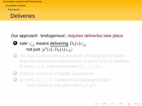
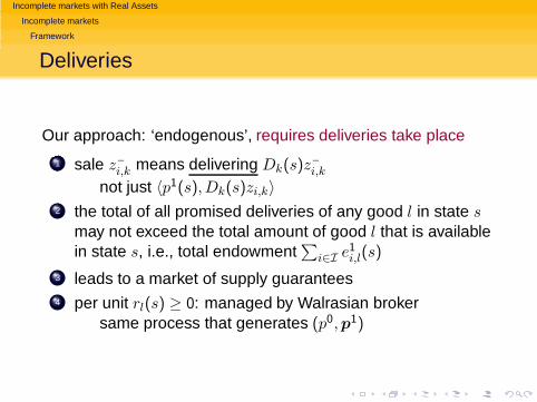
Deliveries
Our approach: ‘endogenous’, requires deliveries take place
1 sale z−
i,k means delivering Dk(s)z−
i,k
not just 〈p1(s),Dk(s)zi,k〉
2 the total of all promised deliveries of any good l in state smay not exceed the total amount of good l that is availablein state s, i.e., total endowment
∑
i∈I e1i,l(s)
3 leads to a market of supply guarantees4 per unit rl(s) ≥ 0: managed by Walrasian broker
same process that generates (p0,p1)
Incomplete markets with Real Assets
Incomplete markets
Framework
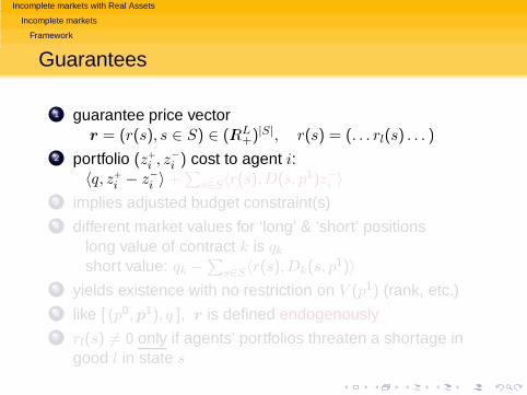
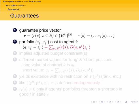
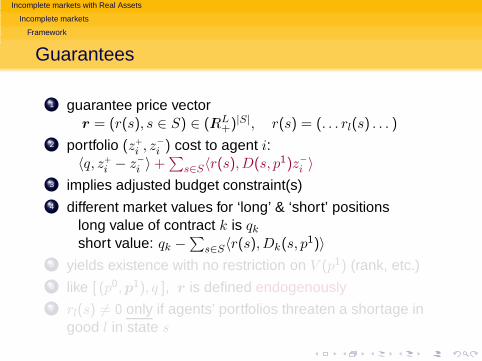
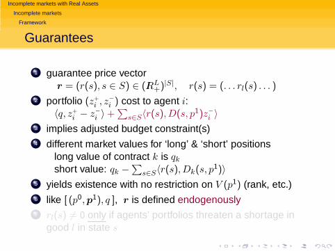
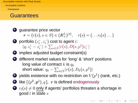
Guarantees
1 guarantee price vectorr = (r(s), s ∈ S) ∈ (IRL
+)|S|, r(s) = (. . . rl(s) . . . )
2 portfolio (z+
i , z−
i ) cost to agent i:〈q, z+
i − z−
i 〉 +∑
s∈S〈r(s),D(s, p1)z−
i 〉
3 implies adjusted budget constraint(s)4 different market values for ‘long’ & ‘short’ positions
long value of contract k is qk
short value: qk −∑
s∈S〈r(s),Dk(s, p1)〉
5 yields existence with no restriction on V (p1) (rank, etc.)6 like [ (p0,p1), q ], r is defined endogenously7 rl(s) 6= 0 only if agents’ portfolios threaten a shortage in
good l in state s
Incomplete markets with Real Assets
Incomplete markets
Framework
Guarantees
1 guarantee price vectorr = (r(s), s ∈ S) ∈ (IRL
+)|S|, r(s) = (. . . rl(s) . . . )
2 portfolio (z+
i , z−
i ) cost to agent i:〈q, z+
i − z−
i 〉 +∑
s∈S〈r(s),D(s, p1)z−
i 〉
3 implies adjusted budget constraint(s)4 different market values for ‘long’ & ‘short’ positions
long value of contract k is qk
short value: qk −∑
s∈S〈r(s),Dk(s, p1)〉
5 yields existence with no restriction on V (p1) (rank, etc.)6 like [ (p0,p1), q ], r is defined endogenously7 rl(s) 6= 0 only if agents’ portfolios threaten a shortage in
good l in state s
Incomplete markets with Real Assets
Incomplete markets
Equilibrium
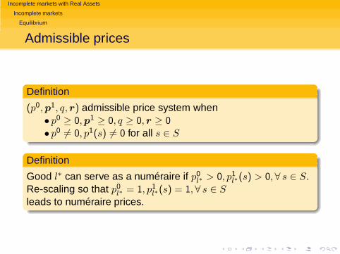
Admissible prices
Definition
(p0,p1, q, r) admissible price system when• p0 ≥ 0,p1 ≥ 0, q ≥ 0, r ≥ 0• p0 6= 0, p1(s) 6= 0 for all s ∈ S
Definition
Good l∗ can serve as a numéraire if p0l∗ > 0, p1
l∗(s) > 0,∀ s ∈ S.Re-scaling so that p0
l∗ = 1, p1l∗(s) = 1,∀ s ∈ S
leads to numéraire prices.
Incomplete markets with Real Assets
Incomplete markets
Equilibrium
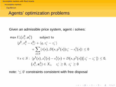
Agents’ optimization problems
Given an admissible price system, agent i solves:
max Ui(x0i ,x
1i ) subject to
〈p0, x0i − e0
i 〉 + 〈q, z+
i − z−
i 〉
+∑
s∈S
〈r(s),D(s, p1(s))z−
i − e1i (s)〉 ≤ 0
∀ s ∈ S : 〈p1(s), x1i (s) − e1
i (s) + D(s, p1(s))[ z+
i − z−
i ]〉 ≤ 0,
(x0i ,x
1i ) ∈ Xi, z+
i ≥ 0, z−
i ≥ 0
note: ‘≤ 0’ constraints consistent with free disposal
Incomplete markets with Real Assets
Incomplete markets
Equilibrium
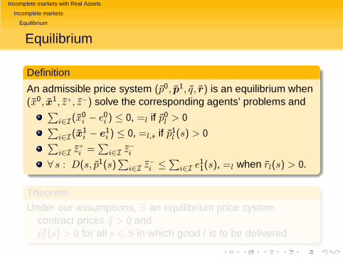
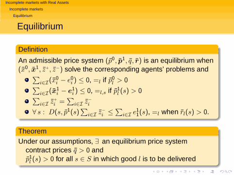
Equilibrium
Definition
An admissible price system (p̄0, p̄1, q̄, r̄) is an equilibrium when(x̄0, x̄1, z̄+, z̄−) solve the corresponding agents’ problems and
∑
i∈I(x̄0i − e0
i ) ≤ 0, =l if p̄0l > 0
∑
i∈I(x̄1i − e1
i ) ≤ 0, =l,s if p̄1l (s) > 0
∑
i∈I z̄+
i =∑
i∈I z̄−
i
∀ s : D(s, p̄1(s)∑
i∈I z̄−
i ≤∑
i∈I e11(s), =l when r̄l(s) > 0.
TheoremUnder our assumptions, ∃ an equilibrium price system
contract prices q̄ > 0 andp̄1
l (s) > 0 for all s ∈ S in which good l is to be delivered
Incomplete markets with Real Assets
Incomplete markets
Equilibrium
Equilibrium
Definition
An admissible price system (p̄0, p̄1, q̄, r̄) is an equilibrium when(x̄0, x̄1, z̄+, z̄−) solve the corresponding agents’ problems and
∑
i∈I(x̄0i − e0
i ) ≤ 0, =l if p̄0l > 0
∑
i∈I(x̄1i − e1
i ) ≤ 0, =l,s if p̄1l (s) > 0
∑
i∈I z̄+
i =∑
i∈I z̄−
i
∀ s : D(s, p̄1(s)∑
i∈I z̄−
i ≤∑
i∈I e11(s), =l when r̄l(s) > 0.
TheoremUnder our assumptions, ∃ an equilibrium price system
contract prices q̄ > 0 andp̄1
l (s) > 0 for all s ∈ S in which good l is to be delivered
Incomplete markets with Real Assets
Incomplete markets
Equilibrium
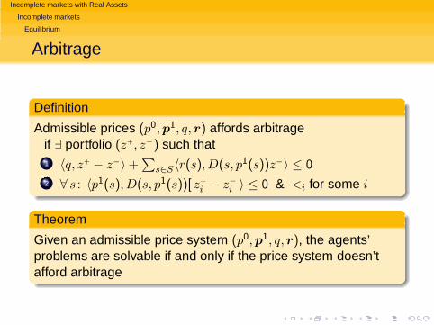
Arbitrage
Definition
Admissible prices (p0,p1, q, r) affords arbitrageif ∃ portfolio (z+, z−) such that1 〈q, z+ − z−〉 +
∑
s∈S〈r(s),D(s, p1(s))z−〉 ≤ 0
2 ∀ s : 〈p1(s),D(s, p1(s))[ z+
i − z−
i 〉 ≤ 0 & <i for some i
Theorem
Given an admissible price system (p0,p1, q, r), the agents’problems are solvable if and only if the price system doesn’tafford arbitrage
Incomplete markets with Real Assets
Incomplete markets
Equilibrium
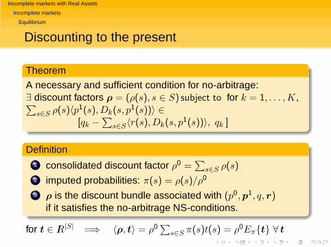
Discounting to the present
Theorem
A necessary and sufficient condition for no-arbitrage:∃ discount factors ρ = (ρ(s), s ∈ S) subject to for k = 1, . . . ,K,∑
s∈S ρ(s)〈p1(s),Dk(s, p1(s))〉 ∈
[qk −∑
s∈S〈r(s),Dk(s, p1(s))〉, qk ]
Definition1 consolidated discount factor ρ0 =
∑
s∈S ρ(s)
2 imputed probabilities: π(s) = ρ(s)/ρ0
3 ρ is the discount bundle associated with (p0,p1, q, r)if it satisfies the no-arbitrage NS-conditions.
for t ∈ IR|S| =⇒ 〈ρ, t〉 = ρ0∑
s∈S π(s)t(s) = ρ0Eπ{t} ∀ t
Incomplete markets with Real Assets
Incomplete markets
Equilibrium
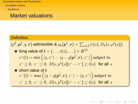
Market valuations
Definition
(p0,p1, q, r)-admissible & gk(p1, r) =
∑
s∈S〈r(s),Dk(s, p1(s))〉
long value of t = (. . . , t(s), . . . ) ∈ IR|S|
v+(t) = min(
〈q, z+〉 − 〈q − g(p1, r), z−〉)
subject to
z+ ≥ 0, z− ≥ 0, D(s, p1(s)[z+ − z−] ≥ t(s) for all s
short value of t
v−(t) = max(
〈q − g(p1, r), z−〉 − 〈q, z+〉)
subject to
z+ ≥ 0, z− ≥ 0, D(s, p1(s)[z+ − z−] ≤ t(s) for all s
Incomplete markets with Real Assets
Incomplete markets
Equilibrium
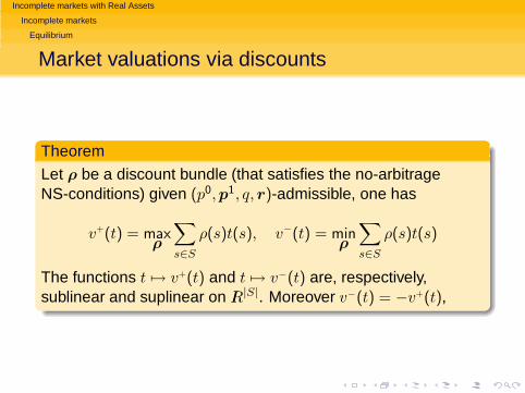
Market valuations via discounts
Theorem
Let ρ be a discount bundle (that satisfies the no-arbitrageNS-conditions) given (p0,p1, q, r)-admissible, one has
v+(t) = maxρ
∑
s∈S
ρ(s)t(s), v−(t) = minρ
∑
s∈S
ρ(s)t(s)
The functions t 7→ v+(t) and t 7→ v−(t) are, respectively,sublinear and suplinear on IR|S|. Moreover v−(t) = −v+(t),
Incomplete markets with Real Assets
Incomplete markets
Equilibrium
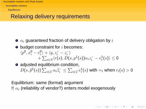
Relaxing delivery requirements
αi guaranteed fraction of delivery obligation by i
budget constraint for i becomes:〈p0, x0
i − e0i 〉 + 〈q, z+
i − z−
i 〉+
∑
s∈S〈r(s),D(s, p1(s))αiz−
i − e1i (s)〉 ≤ 0
adjusted equilibrium condition,D(s, p̄1(s))
∑
i∈I αiz̄−
i ≤∑
i∈I e1i (s) with =l when rl(s) > 0
Equilibrium: same (formal) argument!! αi (reliability of vendor?) enters model exogenously
Incomplete markets with Real Assets
Incomplete markets
Equilibrium
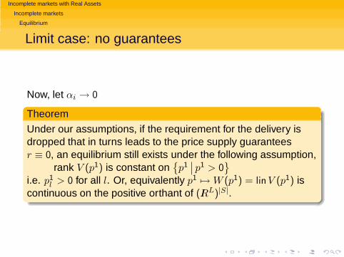
Limit case: no guarantees
Now, let αi → 0
Theorem
Under our assumptions, if the requirement for the delivery isdropped that in turns leads to the price supply guaranteesr ≡ 0, an equilibrium still exists under the following assumption,
rank V (p1) is constant on{
p1∣
∣ p1 > 0}
i.e. p1l > 0 for all l. Or, equivalently p1 7→ W (p1) = linV (p1) is
continuous on the positive orthant of (IRL)|S|.
Incomplete markets with Real Assets
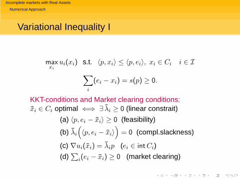
Numerical Approach
Variational Inequality I
maxxi
ui(xi) s.t. 〈p, xi〉 ≤ 〈p, ei〉, xi ∈ Ci i ∈ I
∑
i
(ei − xi) = s(p) ≥ 0.
KKT-conditions and Market clearing conditions:x̄i ∈ Ci optimal ⇐⇒ ∃ λ̄i ≥ 0 (linear constrait)
(a) 〈p, ei − x̄i〉 ≥ 0 (feasibility)
(b) λ̄i
(
〈p, ei − x̄i〉)
= 0 (compl.slackness)
(c) ∇ui(x̄i) = λ̄ip (ei ∈ int Ci)
(d)∑
i(ei − x̄i) ≥ 0 (market clearing)
Incomplete markets with Real Assets
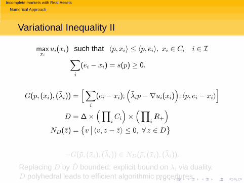
Numerical Approach
Variational Inequality II
maxxi
ui(xi) such that 〈p, xi〉 ≤ 〈p, ei〉, xi ∈ Ci i ∈ I∑
i
(ei − xi) = s(p) ≥ 0.
G(p, (xi), (λ̄i)) =[
∑
i
(ei − xi);(
λ̄ip −∇ui(xi))
; 〈p, ei − xi〉]
D = ∆ ×(
∏
iCi
)
×(
∏
iIR+
)
ND(z̄) ={
v∣
∣ 〈v, z − z̄〉 ≤ 0, ∀ z ∈ D}
−G(p̄, (x̄i), (λ̄i)) ∈ ND(p̄, (x̄i), (λ̄i)).
Replacing D by D̂ bounded: explicit bound on λi via duality.D polyhedral leads to efficient algorithmic procedures
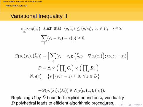
Incomplete markets with Real Assets
Numerical Approach
Variational Inequality II
maxxi
ui(xi) such that 〈p, xi〉 ≤ 〈p, ei〉, xi ∈ Ci i ∈ I∑
i
(ei − xi) = s(p) ≥ 0.
G(p, (xi), (λ̄i)) =[
∑
i
(ei − xi);(
λ̄ip −∇ui(xi))
; 〈p, ei − xi〉]
D = ∆ ×(
∏
iCi
)
×(
∏
iIR+
)
ND(z̄) ={
v∣
∣ 〈v, z − z̄〉 ≤ 0, ∀ z ∈ D}
−G(p̄, (x̄i), (λ̄i)) ∈ ND(p̄, (x̄i), (λ̄i)).
Replacing D by D̂ bounded: explicit bound on λi via duality.D polyhedral leads to efficient algorithmic procedures
Incomplete markets with Real Assets
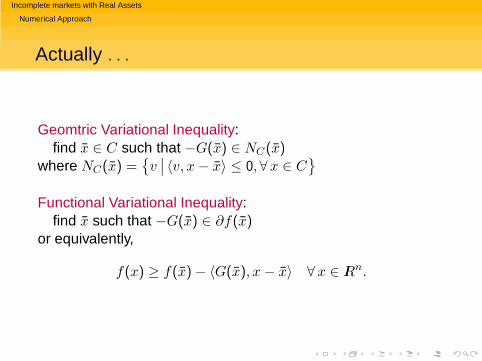
Numerical Approach
Actually . . .
Geomtric Variational Inequality:find x̄ ∈ C such that −G(x̄) ∈ NC(x̄)
where NC(x̄) ={
v∣
∣ 〈v, x − x̄〉 ≤ 0,∀x ∈ C}
Functional Variational Inequality:find x̄ such that −G(x̄) ∈ ∂f(x̄)
or equivalently,
f(x) ≥ f(x̄) − 〈G(x̄), x − x̄〉 ∀x ∈ IRn.
Incomplete markets with Real Assets
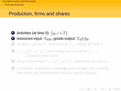
Firms and production
Production, firms and shares
1 Activities (at time 0):{
yi, i ∈ I}
2 resources input: Ti0yi, goods output: Ti1(s)yi
3 auxiliary goods y0′: endowment e0′j,l′
j
, traded @ time 0
4 Yj ={
(y0j , y
0′j ,y1
j
}
technology set for activity j ∈ Jclosed convex cone
5 Share ownership: θj = y0′j,l′
jand θi,j ownership by agent i
6 Examples: production, savings and storage, pre-existingsecurities and investments (bonds, equity shares), . . .
Incomplete markets with Real Assets
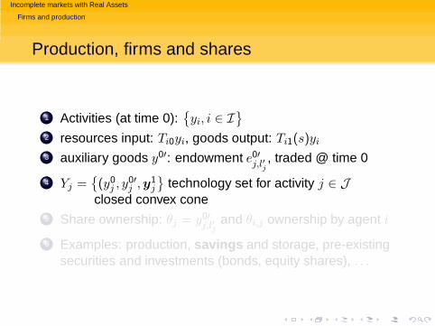
Firms and production
Production, firms and shares
1 Activities (at time 0):{
yi, i ∈ I}
2 resources input: Ti0yi, goods output: Ti1(s)yi
3 auxiliary goods y0′: endowment e0′j,l′
j
, traded @ time 0
4 Yj ={
(y0j , y
0′j ,y1
j
}
technology set for activity j ∈ Jclosed convex cone
5 Share ownership: θj = y0′j,l′
jand θi,j ownership by agent i
6 Examples: production, savings and storage, pre-existingsecurities and investments (bonds, equity shares), . . .
Incomplete markets with Real Assets
Firms and production
Production, firms and shares
1 Activities (at time 0):{
yi, i ∈ I}
2 resources input: Ti0yi, goods output: Ti1(s)yi
3 auxiliary goods y0′: endowment e0′j,l′
j
, traded @ time 0
4 Yj ={
(y0j , y
0′j ,y1
j
}
technology set for activity j ∈ Jclosed convex cone
5 Share ownership: θj = y0′j,l′
jand θi,j ownership by agent i
6 Examples: production, savings and storage, pre-existingsecurities and investments (bonds, equity shares), . . .